design of a solar thermal power-propulsion system for … · master of science thesis design of a...
TRANSCRIPT
Master of Science Thesis
Design of a Solar Thermal Power-PropulsionSystem for a Small Satellite
A feasibility study of a solar thermal hybrid system
J.J. Preijde
29th of January 2015
Faculty of Aerospace Engineering · Delft University of Technology


Design of a Solar Thermal Power-PropulsionSystem for a Small Satellite
A feasibility study of a solar thermal hybrid system
Master of Science Thesis
For obtaining the degree of Master of Science in AerospaceEngineering at Delft University of Technology
J.J. Preijde
29th of January 2015
Faculty of Aerospace Engineering · Delft University of Technology

Copyright © J.J. PreijdeAll rights reserved.
Delft University Of TechnologyDepartment Of
Space Systems Engineering
The undersigned hereby certify that they have read and recommend to the Faculty ofAerospace Engineering for acceptance a thesis entitled “Design of a Solar ThermalPower-Propulsion System for a Small Satellite” by J.J. Preijde in partial fulfillmentof the requirements for the degree of Master of Science.
Dated: 29th of January 2015
Head of department:Prof.dr. E.K.A Gill
Supervisor:A. Cervone
Reader:C.M. De Servi


Summary
Besides chemical, cold gas and electric propulsion, solar thermal propulsion (STP) providesan alternative approach to spacecraft propulsion.This technology can also be adapted to provide power to the spacecraft by converting apart of the totally available thermal energy into electrical energy. If combined, one canbuild a solar thermal power-propulsion hybrid system. This thesis focuses on a systemfor a small satellite with a dry mass of 200 kg and a bus volume of 1 m3.
The propulsion subsystem concerns a primary and secondary solar concentrator, areceiver/absorber cavity (RAC), a heat exchange mechanism between absorber and propellant,a propellant storage and feed system, a thruster chamber and a thruster nozzle.
The power subsystem consists of an interface between the absorber and a heat exchanger,the heat exchanger which heats up the working fluid in the Organic Rankine Cycle (ORC)power subsystem, a turbine which provides the power and a condenser which dissipates apart of the heat in the working fluid. Finally, a small pump is used to force the cold fluidto the heat exchanger and increase the pressure of the fluid.
A Design, Analysis and Optimization (DAO) tool has been built to model the hybridsystem. Results from the tool have yielded performances of particular designs and haveprovided answers whether such a system is feasible and offers advantages over conventionalpower and propulsion subsystems.The DAO model consists of a solar flux and orbit model to calculate the orbit characteristicsand available solar flux. The thermal and thruster models subsequently calculate thetemperature of the thermal nodes of the system as well as the propulsive performance.Nine thermal nodes have been used to calculate the temperatures from solar concentratorsto the interface between absorber and ORC heat exchanger. These nodes have beendivided in a total of 17 sub-nodes.After model integration a long iterative cycle has been performed where different designvariables have been changed to evaluate design-performance relations. These variablesinclude the type of propellant, material choices for the thermal nodes, shape of theabsorber, shape of the thruster nozzle as well as the width and length of the differentnodes. A maximum of three orbits is simulated to limit computing time. Thrust isassumed to be generated during that entire time to achieve a worst-case scenario. Withinthose three orbits eclipse is taken into account. During those eclipse periods propellantflow is interrupted whereas power generation continues.
v

vi Summary
Application of the DAO tool yielded that a conical nozzle produces less thrust than abell-shaped nozzle. In terms of non-cryogenic propellants water and hydrogen respectivelyachieved too low temperatures and a too high storage volume to be practical. This leftliquid ammonia and liquid hydrogen as propellant candidates. Due to the larger lengthof propellant tubing in a spiral configuration of one feed line in comparison to a linearconfiguration of multiple feed lines, the former was selected for the conceptual designs.The conceptual design phase yielded six designs, each set of two with a conical, cylindricalor spherical absorber. Each concept either had ammonia or hydrogen as propellant toallow comparison of the performance of different propellants.Analyzing the scalability of the system in terms of its performance resulted in limitedscalability for output power with a doubling of the power requiring a too large heatdissipation out of the condenser. Also for specific impulse the scalability was limited. Agood scalability however was achieved in terms of the thrust from 1 N originally to atleast 5 N. The assumption here was that no large design changes have to occur to achievehigher performance.
After running the DAO tool for the concepts and making a trade-off, the third conceptwas selected. It has a cylindrical RAC and uses liquid ammonia. The liquid hydrogenoption for the same RAC configuration was deemed infeasible due to the 20-K storagetemperature requirement which is very difficult to achieve in a small satellite.The third concept has a relatively low system complexity, a high thrust and an advantageouslylow system volume estimate. Its main disadvantage however is the low system-specificimpulse meaning it will require more system mass to generate a certain amount of impulse.
The detailed design phase led to a more detailed design and accurate characterization ofthe concept.The decision was made to include an on-axis primary concentrator as this device is easierto model than an off-axis concentrator. A comparison between the two types is beyond thescope of this thesis. The secondary concentrator is a refractive one made of a single-crystalsapphire material. The secondary concentrator casing and the other components are madeof molybdenum since this material has a high thermal conductivity and can cope withtemperatures up to 2800 K.
The casing has a white-paint coating to limit its emissivity and temperature increase dueto external radiation. The pre-cavity chamber connecting the casing and the RAC lid isinsulated with multi-layer insulation (MLI) and fastened and grounded with hook-and-pilefasteners and conductive tape. The RAC lid has a 14 mm molybdenum core and on bothsides a 43-mm thick MLI blanket to insulate the cavity from the rest of the system infront of it.The cylindrical RAC has an outer diameter of 14 cm and a wall thickness of 10.8 mm. Ithas a length of 30 cm. The interior has a high-performance black-paint coating giving itan absorptance of 0.96 and an emissivity of 0.88.Three mounting options for the RAC were traded-off: mounting by aluminium struts,passive orbit disconnect struts (PODS) or encapsulation by MLI. Although the MLIoption preserved the RAC temperature the best it also had the largest mass. Aluminiumstruts caused a large dissipation of RAC heat. PODS were therefore selected. They

Summary vii
maintain the RAC relatively well and the eight struts have a combined mass of only 64 g.
While discussing the propellant feed system, pump-driven and blow-down systems werebriefly compared. Since a pump-fed system would increase the mass ans size of the entiresystem considerably, a blow-down scheme was selected.
For the thruster nozzle a bell-shape was selected due to the smaller loss of thrust comparedto a conical nozzle. After comparing 12 nozzle shapes, a nozzle with an expansion ratioof 300 and a length of 9 cm was designed. The nozzle throat convergence half angle is 25degrees, the throat divergence half angle is 30 degrees and the nozzle exhaust divergencehalf angle is 13.8 degrees. This yielded a specific impulse of 185 s and thrust of 1.31 N.The thruster mass estimate is 0.064 kg. The required propellant mass is 29.3 kg.
The tubing was compartmentalized in three parts, the tubing from propellant tank tothe RAC, the RAC tubing and the tubing from RAC to the thruster. Summing thethree tubing lengths up, resulted in a total tubing length of 9.14 m and an accompanyingtubing mass of 0.914 kg. The pressure loss in the gaseous flow, the liquid flow and dueto acceleration pressure and two-phase flow was summed up to a loss of 128 kPa. If thethruster chamber pressure is 1 bar, the pressure at the tank exit must therefore be atleast 2.28 bar.
A cylindrical propellant tank was designed, since a spherical tank would be impracticalwithin the spacecraft bus. The tank has a volume of 0.052 m3. It has a total length of65 cm and an inner radius of 17.6 cm. The tank wall has a thickness of 1.1 mm with asafety factor of 1.5. The pressurant gas helium must be at a pressure of 11.4 to guaranteethis pressure during the entire blow-down process. The total tank mass is estimated at2.10 kg. Together with the propellant and pressurant gas a total propellant tank massof 31.4 kg was determined. Passive and active thermal control for the propellant tankwas also discussed. Since active thermal control is troublesome to integrate and requiresheavy components, only passive thermal control was used. Three options were analyzedand traded-off. First, an MLI option only was analyzed. Second and third, an MLI with aradiator and an MLI with optical solar reflectors (OSRs) option were looked at. The firstand third option would increase the temperature of the propellant tank beyond the 243-Krequirement. Only the second option maintained a constant temperature. In addition,the radiator could be integrated into the spacecraft bus, saving mass. Therefore, theMLI-radiator option was selected with an insulation mass of 1.4 kg.
Two check vales are used to fill the propellant tank with helium pressurant and ammoniapropellant. A check valve in front of the thruster makes sure a minimum thrust isguaranteed. Two relief valves can evacuate over-pressurized propellant flow if necessarywithout leading to severe attitude disturbances. A solenoid valve and pressure regulatorrespectively control the activation of propellant flow and the pressure down-stream of thepropellant tank. The total valve mass is 3.7 kg.Together with the 25-kg mass for the RAC system this yields a total dry propulsionsubsystem mass of 36 kg.

viii Summary
As stated previously, the power subsystem has four main components: the evaporator,turbine, condenser and pump. The working fluid in the ORC is toluene and the heatinggas to the evaporator is air. The heat transfer between evaporator heating gas channeland the RAC occurs through radiative processes. This saves system volume and massover a conductive heat channel.The heating gas channel has an outer diameter of 3.5 cm and a tube thickness of 2.7 mm.This yields a channel mass of 0.940 kg. The air in the channel is fed into the evaporatorheat exchanger at a pressure of 5 kPa. A plate fin heat exchanger with a mass of 14 kgwas selected to provide the heat exchange between the air and the working fluid.
The micro-turbine was linearly scaled based on turbine literature. The turbine must dealwith a turbine inlet temperature of the toluene of 565 K, an inlet pressure of 13.67 barand a working fluid flow rate of 0.85 g/s. Its rotor diameter would be 1-3 cm and fromlinear scaling a mass of 0.413 kg was determined. The long-term performance and specificdesign of the turbine are matters which will need to be researched and analyzed. Theseissues are however beyond the scope of this thesis.
The condenser is a passive device as an active condenser would increase the mass substantiallyand add another fluid cycle to the spacecraft. The condenser needs to dissipate 573 W toensure a working fluid temperature of 313 K. The heat can be dissipated to space and/orthe spacecraft interior.A box was simulated with a total external area of m2, an emittance of 0.80 and a viewfactor to the surroundings of 0.9. It needed to be kept at a temperature of 15 degreesCelsius, assuming an environment temperature of 173.15 K. A heat of 223 W was requiredfor heating purposes. The condenser therefore needed to dissipate 350 W to space.A condenser conducting channel with a length of 10 cm and a diameter of 16 mm wascalculated to transfer the heat from the condenser to the radiator plate. The condenserouter radius is 8.5 mm and the length over which the working fluid is cooled is 5 cm. Atotal mass of 0.209 kg was calculated for these two components. The radiator plate isincorporated into the bus structure and has an area of 0.4 m2.
A micro-pump is used to increase the pressure of the working fluid to the evaporatingpressure of 13.67 bar and force the fluid from condenser to evaporator. A representativedevice was procured. The device uses 100 mW and has a mass of 0.34 kg. This device isa magnetic drive pump with a maximum speed of 8000 rpm.
For the working fluid feed system, a total tubing length of 1.06 m including a 10% marginfor bends was calculated. The outer tubing diameter is 1.7 cm and the wall has a thicknessof 1.3 mm. The Al-6061 aluminium alloy was selected for the tubing material as the fluidtemperature does not exceed 400 K. This yielded a tubing mass of 0.184 kg.Including a 20% design margin to take into account unknowns and the unknown air andtoluene mass, the total power subsystem mass became 19.3 kg.
The total wet system mass then became 84.8 kg. After running the model for a final

Summary ix
time, a thrust, specific impulse and power was generated of respectively 1.31 N, 185 s and115 W. The system had a maximum daylight efficiency in the third orbit of 37% and aminimum efficiency in eclipse of 17%. The system-specific impulse was 65 s.An estimate of 0.83 m3 was given for the practical space left in the spacecraft bus afterhybrid system integration.
Compared to a conventional system which generates the same kind of power, thrustand specific impulse, the hybrid system mass were way more than the 30.9 kg for theconventional system. Furthermore, the system-specific impulse was lower than the 123s for the conventional system. The major operational advantage of the hybrid systemhowever is that it can generate power during both daylight and eclipse, saving the needfor batteries.For larger satellites with a larger bus and mass this system will be more appropriate asit will need a relatively smaller fraction of the bus volume and mass due to non-linearscaling of the system.
After this design and feasibility study, the research questions posed at the beginning couldbe answered.If one looks at the difference in thrust and specific impulse when the propellant is changedfrom ammonia to hydrogen, the thrust decreased only marginally. The specific impulsehowever increased by a factor of 3.2 to 4.0. Water increased the specific impulse by 9%and nitrogen was representative of the performance of ammonia. The latter howeverrequires a large storage volume. Nitrogen can thus be used for testing purposes when nocryogenic equipment is available.One could therefore conclude that using liquid hydrogen creates a lighter and smallersystem with respect to the use of liquid ammonia. The concepts which use ammoniahowever require a smaller primary concentrator.
The concepts which use hydrogen and have a conical or spherical RAC provided the fastestand largest heat exchange between the RAC and the propellant.A radiative interface between the RAC and evaporator heating gas conduit had a smallermass as it required no physical connection between the RAC and the conduit. It wastherefore the most appropriate for the design considered.It was determined after a number of iterative simulations that appreciable scalabilitywithin the same system is only achieved for thrust; the power and specific impulse canbarely be scaled up.
Equation 5.5 gives the efficiency equation for the hybrid system and includes the inputsolar power, thrust, thruster equivalent exhaust velocity and the output turbine power.To increase the measure of efficiency for the same ORC power output one should increasethe exhaust velocity by increasing the propellant temperature. Furthermore, the nozzleshape can be changed to limit thrust loss.The hydrogen concepts generated a daylight efficiency of 9% versus an efficiency of 29-42%for the ammonia concepts. The ammonia concepts offered greater efficiency in eclipse aswell; they had an efficiency in the range of 13-19% whereas the hydrogen concepts offeredonly 4% efficiency.

x Summary

Acknowledgements
I wish to thank the following individuals for the help they provided me during my thesisresearch:
Angelo Cervone, for the supervision and feedback on my thesis as well as the researchprocess;
Adam Head and Sebastian Bahamonde, for the help in applying and integrating theORCHID-VPE model into the thesis model;
and prof. Piero Colonna, for providing additional information on ORC processes.
J.J. Preijde Delft, The Netherlands29th of January 2015
xi

xii Acknowledgements

Contents
Summary v
Acknowledgements xi
List of Figures xxii
List of Tables xxiv
Nomenclature xxv
Glossary xxxi
1 Introduction 1
2 Research framework 3
2.1 Research questions . . . . . . . . . . . . . . . . . . . . . . . . . . . . . . . 3
2.2 Objectives . . . . . . . . . . . . . . . . . . . . . . . . . . . . . . . . . . . . 4
2.3 Operational scenarios . . . . . . . . . . . . . . . . . . . . . . . . . . . . . 5
2.4 System requirements . . . . . . . . . . . . . . . . . . . . . . . . . . . . . . 6
3 Design, Analysis and Optimization Tool 9
3.1 Orbit and solar flux model . . . . . . . . . . . . . . . . . . . . . . . . . . . 10
3.1.1 Orbit model . . . . . . . . . . . . . . . . . . . . . . . . . . . . . . . 10
3.1.2 Solar flux model . . . . . . . . . . . . . . . . . . . . . . . . . . . . 12
3.2 Thermal model . . . . . . . . . . . . . . . . . . . . . . . . . . . . . . . . . 13
3.2.1 Introduction . . . . . . . . . . . . . . . . . . . . . . . . . . . . . . 13
3.2.2 Geometries and properties of nodes . . . . . . . . . . . . . . . . . . 15
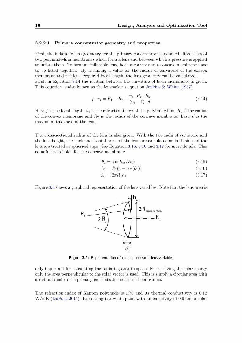
3.2.2.1 Primary concentrator geometry and properties . . . . . . 16
3.2.2.2 Secondary concentrator geometry and properties . . . . . 17
3.2.2.3 RAC geometry and properties . . . . . . . . . . . . . . . 17
3.2.3 Tubing configurations . . . . . . . . . . . . . . . . . . . . . . . . . 19
3.2.3.1 Spiral tubing configuration . . . . . . . . . . . . . . . . . 19
3.2.3.2 Linear tubing configuration . . . . . . . . . . . . . . . . . 20
3.2.4 Heat conducting channel and evaporator . . . . . . . . . . . . . . . 21
3.2.5 View factors . . . . . . . . . . . . . . . . . . . . . . . . . . . . . . 21
xiii

xiv Contents
3.2.6 Gebhart factors and thermal couplings . . . . . . . . . . . . . . . . 22
3.2.7 Convective heat flow . . . . . . . . . . . . . . . . . . . . . . . . . . 23
3.2.7.1 Nusselt, Prandtl and Reynolds numbers . . . . . . . . . . 23
3.2.8 Flow properties in tubing . . . . . . . . . . . . . . . . . . . . . . . 23
3.2.9 Temperature calculations . . . . . . . . . . . . . . . . . . . . . . . 24
3.2.10 Pressure losses . . . . . . . . . . . . . . . . . . . . . . . . . . . . . 26
3.2.10.1 Single-phase flow friction pressure loss . . . . . . . . . . . 27
3.2.10.2 Two-phase flow friction pressure loss . . . . . . . . . . . . 28
3.2.10.3 Acceleration pressure loss . . . . . . . . . . . . . . . . . . 29
3.3 Thruster Model . . . . . . . . . . . . . . . . . . . . . . . . . . . . . . . . . 29
3.3.1 Introduction . . . . . . . . . . . . . . . . . . . . . . . . . . . . . . 29
3.3.2 Nozzle shape . . . . . . . . . . . . . . . . . . . . . . . . . . . . . . 29
3.3.2.1 Conical nozzle . . . . . . . . . . . . . . . . . . . . . . . . 30
3.3.2.2 Bell-shaped nozzle . . . . . . . . . . . . . . . . . . . . . . 30
3.3.3 Nozzle critical flow conditions . . . . . . . . . . . . . . . . . . . . . 31
3.3.4 Chamber flow conditions . . . . . . . . . . . . . . . . . . . . . . . . 32
3.3.5 Thruster and propulsion subsystem performance . . . . . . . . . . 32
3.4 Verification and validation . . . . . . . . . . . . . . . . . . . . . . . . . . . 34
3.4.1 Thrust, specific impulse and mass flow validation . . . . . . . . . . 35
3.4.2 Temperature validation . . . . . . . . . . . . . . . . . . . . . . . . 36
3.5 Observations . . . . . . . . . . . . . . . . . . . . . . . . . . . . . . . . . . 39
3.5.1 Increasing convection area . . . . . . . . . . . . . . . . . . . . . . . 39
3.5.2 Increasing cavity dimensions . . . . . . . . . . . . . . . . . . . . . 40
3.5.3 Too large primary concentrator . . . . . . . . . . . . . . . . . . . . 41
3.5.4 Increasing power output . . . . . . . . . . . . . . . . . . . . . . . . 42
3.5.5 Decreasing propellant mass flow . . . . . . . . . . . . . . . . . . . 42
3.5.6 Applying insulation around RAC . . . . . . . . . . . . . . . . . . . 42
3.5.7 Conclusions concerning observations . . . . . . . . . . . . . . . . . 44
4 Organic Rankine Cycles 47
4.1 Working principles . . . . . . . . . . . . . . . . . . . . . . . . . . . . . . . 47
4.2 Condenser performance . . . . . . . . . . . . . . . . . . . . . . . . . . . . 50
5 Conceptual design 53
5.1 Conceptual system requirements and assumptions . . . . . . . . . . . . . . 53
5.1.1 Requirements . . . . . . . . . . . . . . . . . . . . . . . . . . . . . . 53
5.1.2 Assumptions . . . . . . . . . . . . . . . . . . . . . . . . . . . . . . 54
5.1.2.1 Mass estimates . . . . . . . . . . . . . . . . . . . . . . . . 54
5.1.2.2 RAC and interfaces . . . . . . . . . . . . . . . . . . . . . 55
5.1.2.3 Thermal nodes and tubing conditions . . . . . . . . . . . 55
5.1.2.4 External fluxes and temperatures . . . . . . . . . . . . . 56

Contents xv
5.2 General design considerations . . . . . . . . . . . . . . . . . . . . . . . . . 59
5.2.1 System efficiency . . . . . . . . . . . . . . . . . . . . . . . . . . . . 59
5.2.2 Materials and constituent fluids and gases . . . . . . . . . . . . . . 60
5.2.3 Nozzle shape . . . . . . . . . . . . . . . . . . . . . . . . . . . . . . 61
5.2.4 Tubing configuration . . . . . . . . . . . . . . . . . . . . . . . . . . 63
5.2.5 Power subsystem . . . . . . . . . . . . . . . . . . . . . . . . . . . . 64
5.3 Concepts . . . . . . . . . . . . . . . . . . . . . . . . . . . . . . . . . . . . 66
5.3.1 Thermal nodes and summary of the concepts . . . . . . . . . . . . 66
5.3.2 Concept 1 . . . . . . . . . . . . . . . . . . . . . . . . . . . . . . . . 67
5.3.2.1 Performance with water as non-cryogenic propellant . . . 70
5.3.2.2 Performance with nitrogen as non-cryogenic propellant . 71
5.3.3 Concept 2 . . . . . . . . . . . . . . . . . . . . . . . . . . . . . . . . 72
5.3.4 Concept 3 . . . . . . . . . . . . . . . . . . . . . . . . . . . . . . . . 75
5.3.5 Concept 4 . . . . . . . . . . . . . . . . . . . . . . . . . . . . . . . . 77
5.3.6 Concept 5 . . . . . . . . . . . . . . . . . . . . . . . . . . . . . . . . 80
5.3.7 Concept 6 . . . . . . . . . . . . . . . . . . . . . . . . . . . . . . . . 83
5.4 Mass and size comparison of concepts . . . . . . . . . . . . . . . . . . . . 85
5.4.1 Mass of the concepts . . . . . . . . . . . . . . . . . . . . . . . . . . 85
5.4.2 Size of the concepts . . . . . . . . . . . . . . . . . . . . . . . . . . 86
5.5 Performance comparison of concepts . . . . . . . . . . . . . . . . . . . . . 88
5.6 Scalability . . . . . . . . . . . . . . . . . . . . . . . . . . . . . . . . . . . . 89
5.6.1 Power . . . . . . . . . . . . . . . . . . . . . . . . . . . . . . . . . . 90
5.6.2 Thrust . . . . . . . . . . . . . . . . . . . . . . . . . . . . . . . . . . 90
5.6.3 Specific impulse . . . . . . . . . . . . . . . . . . . . . . . . . . . . . 91
5.7 Thermal stresses . . . . . . . . . . . . . . . . . . . . . . . . . . . . . . . . 92
5.8 Overall comparison of concepts . . . . . . . . . . . . . . . . . . . . . . . . 94
5.8.1 Performance . . . . . . . . . . . . . . . . . . . . . . . . . . . . . . 94
5.8.2 Thermal stresses and expansions . . . . . . . . . . . . . . . . . . . 94
5.9 Conceptual trade-off . . . . . . . . . . . . . . . . . . . . . . . . . . . . . . 95
5.9.1 Trade-off criteria . . . . . . . . . . . . . . . . . . . . . . . . . . . . 95
5.9.1.1 Weighting factors . . . . . . . . . . . . . . . . . . . . . . 95
5.9.1.2 System volume criterion . . . . . . . . . . . . . . . . . . . 96
5.9.1.3 System complexity criterion . . . . . . . . . . . . . . . . 97
5.9.2 Trade-off and selection of final concept . . . . . . . . . . . . . . . . 98

xvi Contents
6 Detailed design 101
6.1 System architecture and design options . . . . . . . . . . . . . . . . . . . . 101
6.2 Propulsion subsystem . . . . . . . . . . . . . . . . . . . . . . . . . . . . . 102
6.2.1 Functional and physical architecture . . . . . . . . . . . . . . . . . 102
6.2.2 Secondary concentrator . . . . . . . . . . . . . . . . . . . . . . . . 104
6.2.2.1 Concentrator lens . . . . . . . . . . . . . . . . . . . . . . 104
6.2.2.2 Concentrator casing . . . . . . . . . . . . . . . . . . . . . 105
6.2.3 Pre-cavity chamber . . . . . . . . . . . . . . . . . . . . . . . . . . . 106
6.2.4 RAC and RAC lid . . . . . . . . . . . . . . . . . . . . . . . . . . . 106
6.2.4.1 PODS . . . . . . . . . . . . . . . . . . . . . . . . . . . . . 108
6.2.4.2 Aluminium struts . . . . . . . . . . . . . . . . . . . . . . 110
6.2.4.3 MLI and fasteners . . . . . . . . . . . . . . . . . . . . . . 111
6.2.4.4 Comparison of mounting options . . . . . . . . . . . . . . 111
6.2.4.5 Mass budget . . . . . . . . . . . . . . . . . . . . . . . . . 112
6.2.5 Propellant feed system . . . . . . . . . . . . . . . . . . . . . . . . . 113
6.2.5.1 Thruster . . . . . . . . . . . . . . . . . . . . . . . . . . . 114
6.2.5.2 Propellant tubing . . . . . . . . . . . . . . . . . . . . . . 115
6.2.5.2.1 Pressure loss for liquid propellant . . . . . . . . 117
6.2.5.2.2 Pressure loss for gaseous propellant . . . . . . . 117
6.2.5.2.3 Two-phase propellant and acceleration pressurelosses . . . . . . . . . . . . . . . . . . . . . . . . 118
6.2.5.2.4 Total pressure loss . . . . . . . . . . . . . . . . . 118
6.2.5.3 Propellant tank . . . . . . . . . . . . . . . . . . . . . . . 120
6.2.5.4 Propellant tank thermal control . . . . . . . . . . . . . . 121
6.2.5.4.1 Propellant tank covered in MLI . . . . . . . . . 122
6.2.5.4.2 Propellant tank covered in MLI and interfacingwith radiator panel . . . . . . . . . . . . . . . . 123
6.2.5.4.3 Propellant tank covered in MLI and covered withOSRs . . . . . . . . . . . . . . . . . . . . . . . . 125
6.2.5.4.4 Comparison of propellant tank thermal controloptions . . . . . . . . . . . . . . . . . . . . . . . 125
6.2.5.5 Valves . . . . . . . . . . . . . . . . . . . . . . . . . . . . . 126
6.2.5.5.1 Solenoid valves . . . . . . . . . . . . . . . . . . . 126
6.2.5.5.2 Pressure regulator valve . . . . . . . . . . . . . . 126
6.2.5.5.3 Pressure relief valves . . . . . . . . . . . . . . . . 127
6.2.5.5.4 Check valves . . . . . . . . . . . . . . . . . . . . 127
6.2.6 Mass budget . . . . . . . . . . . . . . . . . . . . . . . . . . . . . . 127
6.3 Power subsystem . . . . . . . . . . . . . . . . . . . . . . . . . . . . . . . . 128
6.3.1 Functional and physical architecture . . . . . . . . . . . . . . . . . 128
6.3.2 Evaporator . . . . . . . . . . . . . . . . . . . . . . . . . . . . . . . 129
6.3.2.1 Heat transfer through conduction . . . . . . . . . . . . . 130
6.3.2.2 Heat transfer through radiation . . . . . . . . . . . . . . 130

Contents xvii
6.3.2.3 Comparison of heat transfer options . . . . . . . . . . . . 131
6.3.2.4 Evaporator heating gas channel properties . . . . . . . . 131
6.3.2.5 Evaporator heat exchanger . . . . . . . . . . . . . . . . . 132
6.3.3 Turbine . . . . . . . . . . . . . . . . . . . . . . . . . . . . . . . . . 132
6.3.4 Condenser . . . . . . . . . . . . . . . . . . . . . . . . . . . . . . . . 133
6.3.5 Pump . . . . . . . . . . . . . . . . . . . . . . . . . . . . . . . . . . 135
6.3.6 Working fluid feed system . . . . . . . . . . . . . . . . . . . . . . . 135
6.3.7 Mass budget . . . . . . . . . . . . . . . . . . . . . . . . . . . . . . 135
6.4 System integration . . . . . . . . . . . . . . . . . . . . . . . . . . . . . . . 136
6.5 Comparison with conventional system . . . . . . . . . . . . . . . . . . . . 138
6.5.1 Conventional power and propulsion system . . . . . . . . . . . . . 139
6.5.1.1 Power subsystem . . . . . . . . . . . . . . . . . . . . . . . 139
6.5.1.2 Propulsion subsystem . . . . . . . . . . . . . . . . . . . . 140
6.5.2 Performance comparison . . . . . . . . . . . . . . . . . . . . . . . . 140
7 Answering research questions 143
8 Conclusions and recommendations 147
8.1 Conclusions . . . . . . . . . . . . . . . . . . . . . . . . . . . . . . . . . . . 147
8.2 Recommendations . . . . . . . . . . . . . . . . . . . . . . . . . . . . . . . 148
8.2.1 Test recommendations . . . . . . . . . . . . . . . . . . . . . . . . . 148
8.2.2 Research recommendations . . . . . . . . . . . . . . . . . . . . . . 149
References 151
A View factors 159
A.1 Node 1 to Node 5 . . . . . . . . . . . . . . . . . . . . . . . . . . . . . . . . 159
A.2 Node 6 . . . . . . . . . . . . . . . . . . . . . . . . . . . . . . . . . . . . . . 161
A.2.1 Conical RAC . . . . . . . . . . . . . . . . . . . . . . . . . . . . . . 161
A.2.2 Cylindrical RAC . . . . . . . . . . . . . . . . . . . . . . . . . . . . 162
A.2.3 Spherical RAC . . . . . . . . . . . . . . . . . . . . . . . . . . . . . 163
A.3 View factors to space . . . . . . . . . . . . . . . . . . . . . . . . . . . . . . 164
B Design parameters for conceptual designs 165

xviii Contents

List of Figures
2.1 Representative sequence diagram for propulsion subsystem . . . . . . . . . 5
2.2 Representative sequence diagram for power subsystem . . . . . . . . . . . 6
3.1 Process diagram for DAO tool . . . . . . . . . . . . . . . . . . . . . . . . . 9
3.2 Orbit angles to determine solar flux Larson & Wertz (2005) . . . . . . . . 11
3.3 Plot for the available power and the eclipse time over one year for thereference mission . . . . . . . . . . . . . . . . . . . . . . . . . . . . . . . . 13
3.4 Schematic of the thermal model node network . . . . . . . . . . . . . . . . 15
3.5 Representation of the concentrator lens variables . . . . . . . . . . . . . . 16
3.6 Representation of the RAC variables . . . . . . . . . . . . . . . . . . . . . 18
3.7 Representation of the spiral tubing variables . . . . . . . . . . . . . . . . . 20
3.8 Process diagram for thermal model . . . . . . . . . . . . . . . . . . . . . . 27
3.9 Two-phase flow region identification (McKetta Jr. 1992) . . . . . . . . . . 28
3.10 Representation of nozzle shape . . . . . . . . . . . . . . . . . . . . . . . . 30
3.11 Process diagram for thruster model . . . . . . . . . . . . . . . . . . . . . . 34
3.12 Leenders & Zandbergen (2008) test results . . . . . . . . . . . . . . . . . . 35
3.13 Instability of the initial propellant temperature values . . . . . . . . . . . 37
3.14 Temperatures for the DUT concept as modelled by the DAO tool . . . . . 38
3.15 Final propellant temperature for different number of spiral tubing turns . 40
3.16 Final propellant temperature for different tubing diameters . . . . . . . . 40
3.17 Final propellant temperature for different RAC diameters . . . . . . . . . 40
3.18 Final propellant temperature for different RAC configurations . . . . . . . 40
3.19 RAC and final propellant temperatures for different primary concentratorand cavity sizes . . . . . . . . . . . . . . . . . . . . . . . . . . . . . . . . . 41
3.20 Secondary concentrator temperature with and without thermal straps . . 42
3.21 Cavity, final propellant and ORC working fluid temperatures at 100 W and150 W power output . . . . . . . . . . . . . . . . . . . . . . . . . . . . . . 43
3.22 Final propellant temperatures with different throat radii . . . . . . . . . . 44
3.23 RAC and final propellant temperatures with and without RAC insulation 45
4.1 Temperature versus entropy plot for simple ORC (Saleh et al. 2007) . . . 48
4.2 Schematic for a solar powered ORC system (Wang et al. 2014) . . . . . . 48
xix

xx List of Figures
4.3 Schematic showing measurement points of enthalpy states (Kapooria et al.2008) . . . . . . . . . . . . . . . . . . . . . . . . . . . . . . . . . . . . . . . 49
5.1 Schematic of the heating gas channel and RAC interface . . . . . . . . . . 56
5.2 Thermal node temperatures for Concept 1 with continuous propellant flowafter flow initialisation . . . . . . . . . . . . . . . . . . . . . . . . . . . . . 57
5.3 Thermal node temperatures for Concept 1 with tungsten components . . 61
5.4 Conical nozzle design . . . . . . . . . . . . . . . . . . . . . . . . . . . . . . 62
5.5 Bell-shaped nozzle design . . . . . . . . . . . . . . . . . . . . . . . . . . . 62
5.6 Propellant flow velocity in the conical nozzle for Concept 1 . . . . . . . . 63
5.7 Propellant flow velocity in the bell-shaped nozzle for Concept 1 . . . . . . 63
5.8 Temperature of thermal nodes for Concept 3 with a linear configurationwith 20 propellant tubes . . . . . . . . . . . . . . . . . . . . . . . . . . . . 64
5.9 ORC thermal efficiency versus evaporating pressure for Concept 1 . . . . 65
5.10 Concept schematic with conical RAC configuration . . . . . . . . . . . . . 67
5.11 Temperature of thermal nodes for Concept 1 . . . . . . . . . . . . . . . . 68
5.12 Thermal mesh rear view at 60 minutes after model initialisation for Concept 1 68
5.13 Thermal mesh front view at 60 minutes after model initialisation for Concept1 . . . . . . . . . . . . . . . . . . . . . . . . . . . . . . . . . . . . . . . . . 68
5.14 Thrust and power generation for Concept 1 . . . . . . . . . . . . . . . . . 69
5.15 Specific impulse for Concept 1 . . . . . . . . . . . . . . . . . . . . . . . . . 69
5.16 System efficiency for Concept 1 . . . . . . . . . . . . . . . . . . . . . . . . 69
5.17 Mean dissipated heat out of ORC condenser for Concept 1 . . . . . . . . . 70
5.18 Thermal node temperatures for Concept 1 with water as propellant . . . . 71
5.19 Thermal node temperatures for Concept 1 with nitrogen as propellant . . 72
5.20 Illustration of thermal straps interfaced with the secondary concentrator . 73
5.22 Thermal mesh rear view at 60 minutes after model initialisation for Concept 2 73
5.23 Thermal mesh front view at 60 minutes after model initialisation for Concept2 . . . . . . . . . . . . . . . . . . . . . . . . . . . . . . . . . . . . . . . . . 73
5.21 Temperature of thermal nodes for Concept 2 . . . . . . . . . . . . . . . . 74
5.24 Thrust and power generation for Concept 2 . . . . . . . . . . . . . . . . . 74
5.25 Specific impulse for Concept 2 . . . . . . . . . . . . . . . . . . . . . . . . . 74
5.26 System efficiency for Concept 2 . . . . . . . . . . . . . . . . . . . . . . . . 75
5.27 Mean dissipated heat out of ORC condenser for Concept 2 . . . . . . . . . 75
5.28 Temperature of thermal nodes for Concept 3 . . . . . . . . . . . . . . . . 76
5.29 Thermal mesh rear view at 60 minutes after model initialisation for Concept 3 76
5.30 Thermal mesh front view at 60 minutes after model initialisation for Concept3 . . . . . . . . . . . . . . . . . . . . . . . . . . . . . . . . . . . . . . . . . 76
5.31 Thrust and power generation for Concept 3 . . . . . . . . . . . . . . . . . 77
5.32 Specific impulse for Concept 3 . . . . . . . . . . . . . . . . . . . . . . . . . 77
5.33 System efficiency for Concept 3 . . . . . . . . . . . . . . . . . . . . . . . . 77
5.34 Mean dissipated heat out of ORC condenser for Concept 3 . . . . . . . . . 78

List of Figures xxi
5.35 Temperature of thermal nodes for Concept 4 . . . . . . . . . . . . . . . . 78
5.36 Thermal mesh rear view at 60 minutes after model initialisation for Concept 4 79
5.37 Thermal mesh front view at 60 minutes after model initialisation for Concept4 . . . . . . . . . . . . . . . . . . . . . . . . . . . . . . . . . . . . . . . . . 79
5.38 Thrust and power generation for Concept 4 . . . . . . . . . . . . . . . . . 79
5.39 Specific impulse for Concept 4 . . . . . . . . . . . . . . . . . . . . . . . . . 79
5.40 System efficiency and effective exhaust velocity for Concept 4 . . . . . . . 80
5.41 Mean dissipated heat out of ORC condenser for Concept 4 . . . . . . . . . 80
5.42 Temperature of thermal nodes for Concept 5 . . . . . . . . . . . . . . . . 81
5.43 Thermal mesh rear view at 60 minutes after model initialisation for Concept 5 81
5.44 Thermal mesh front view at 60 minutes after model initialisation for Concept5 . . . . . . . . . . . . . . . . . . . . . . . . . . . . . . . . . . . . . . . . . 81
5.45 Thrust and power generation for Concept 5 . . . . . . . . . . . . . . . . . 82
5.46 Specific impulse for Concept 5 . . . . . . . . . . . . . . . . . . . . . . . . . 82
5.47 System efficiency for Concept 5 . . . . . . . . . . . . . . . . . . . . . . . . 82
5.48 Mean dissipated heat out of ORC condenser for Concept 5 . . . . . . . . . 83
5.49 Temperature of thermal nodes for Concept 6 . . . . . . . . . . . . . . . . 83
5.50 Thermal mesh rear view at 60 minutes after model initialisation for Concept 6 84
5.51 Thermal mesh front view at 60 minutes after model initialisation for Concept6 . . . . . . . . . . . . . . . . . . . . . . . . . . . . . . . . . . . . . . . . . 84
5.52 Thrust and power generation for Concept 6 . . . . . . . . . . . . . . . . . 84
5.53 Specific impulse for Concept 6 . . . . . . . . . . . . . . . . . . . . . . . . . 84
5.54 System efficiency for Concept 6 . . . . . . . . . . . . . . . . . . . . . . . . 85
5.55 Mean dissipated heat out of ORC condenser for Concept 6 . . . . . . . . . 85
5.56 Illustration of the system’s footprint . . . . . . . . . . . . . . . . . . . . . 86
5.57 Propellant tank temperature for Concept 2 . . . . . . . . . . . . . . . . . 98
5.58 Propellant tank temperature with passive radiator cooling . . . . . . . . . 98
6.1 System architecture and design options . . . . . . . . . . . . . . . . . . . . 102
6.2 Hatley-Pirbhai diagram for propulsion subsystem . . . . . . . . . . . . . . 103
6.3 Propulsion subsystem physical architecture . . . . . . . . . . . . . . . . . 103
6.4 Temperature profile for Concept 3 with 15 thermal straps attached to thesecondary concentrator lens . . . . . . . . . . . . . . . . . . . . . . . . . . 105
6.5 Schematic for secondary concentrator assembly . . . . . . . . . . . . . . . 106
6.6 Schematic for pre-cavity chamber assembly . . . . . . . . . . . . . . . . . 107
6.7 Schematic for PODS (Plachta et al. 2006) . . . . . . . . . . . . . . . . . . 108
6.8 Cross-sectional schematic for RAC assembly . . . . . . . . . . . . . . . . . 109
6.9 Rear-view schematic for RAC assembly . . . . . . . . . . . . . . . . . . . 109
6.10 Temperature profile for Concept 3 with PODS . . . . . . . . . . . . . . . 110
6.11 Temperature profile for Concept 3 with Al 6061-rods between mountingframe and RAC . . . . . . . . . . . . . . . . . . . . . . . . . . . . . . . . . 111
6.12 Temperature profile for Concept 3 with 10-cm thick MLI around RAC . . 112

xxii List of Figures
6.13 Nozzle length-exhaust diameter ratio versus thrust . . . . . . . . . . . . . 115
6.14 Schematic for propellant tubing from propellant tank to RAC . . . . . . . 116
6.15 Schematic for propellant tubing fasteners . . . . . . . . . . . . . . . . . . 119
6.16 Schematic for radiator-propellant tank interface . . . . . . . . . . . . . . . 124
6.17 System architecture of the propellant feed system . . . . . . . . . . . . . . 128
6.18 Hatley-Pirbhai diagram for power subsystem . . . . . . . . . . . . . . . . 129
6.19 Propulsion subsystem physical architecture . . . . . . . . . . . . . . . . . 129
6.20 Schematic for heat exchange options between RAC and heating gas channel 131
6.21 Temperature profile for detailed design . . . . . . . . . . . . . . . . . . . . 137
6.22 Thrust and power for detailed design . . . . . . . . . . . . . . . . . . . . . 138
6.23 Specific impulse for detailed design . . . . . . . . . . . . . . . . . . . . . . 138
6.24 System efficiency for detailed design . . . . . . . . . . . . . . . . . . . . . 138

List of Tables
2.1 System requirements . . . . . . . . . . . . . . . . . . . . . . . . . . . . . . 7
2.2 Functional requirements coupled to operational scenarios . . . . . . . . . . 8
3.1 Mission input parameters . . . . . . . . . . . . . . . . . . . . . . . . . . . 10
3.2 Model input variables for validation (Leenders & Zandbergen 2008) . . . 36
3.3 Comparison of model and test performance . . . . . . . . . . . . . . . . . 36
3.4 Comparison of model and test temperatures . . . . . . . . . . . . . . . . . 38
5.1 Maximum operating temperatures for thermal nodes . . . . . . . . . . . . 54
5.2 Reference mass budgets for small satellites . . . . . . . . . . . . . . . . . . 54
5.3 Performance comparison between a conical and bell-shape nozzle for thesame hybrid system . . . . . . . . . . . . . . . . . . . . . . . . . . . . . . 62
5.4 Summary of the conceptual designs . . . . . . . . . . . . . . . . . . . . . . 67
5.5 Component thickness . . . . . . . . . . . . . . . . . . . . . . . . . . . . . . 68
5.6 Mass comparison of the concepts . . . . . . . . . . . . . . . . . . . . . . . 86
5.7 Estimate of the footprint of the concepts . . . . . . . . . . . . . . . . . . . 87
5.8 Size comparison of the concepts . . . . . . . . . . . . . . . . . . . . . . . . 88
5.9 Performance comparison of the concepts . . . . . . . . . . . . . . . . . . . 88
5.10 System-specific impulse and related variables for the concepts . . . . . . . 89
5.11 Scalability results in terms of power . . . . . . . . . . . . . . . . . . . . . 90
5.12 Scalability results in terms of thrust . . . . . . . . . . . . . . . . . . . . . 91
5.13 Maximum thermal stresses for each concept’s thermal nodes in GPa . . . 92
5.14 Maximum thermal expansion in axial and radial direction for each concept’sthermal nodes in mm . . . . . . . . . . . . . . . . . . . . . . . . . . . . . . 93
5.15 Trade-off criteria comparison matrix . . . . . . . . . . . . . . . . . . . . . 96
5.16 System volume estimate of concepts . . . . . . . . . . . . . . . . . . . . . 97
5.17 Concepts trade-off . . . . . . . . . . . . . . . . . . . . . . . . . . . . . . . 99
6.1 Mass budget for RAC system . . . . . . . . . . . . . . . . . . . . . . . . . 113
6.2 Final comparison of nozzle shapes . . . . . . . . . . . . . . . . . . . . . . 114
6.3 Pressure losses . . . . . . . . . . . . . . . . . . . . . . . . . . . . . . . . . 119
6.4 MLI performance . . . . . . . . . . . . . . . . . . . . . . . . . . . . . . . . 124
6.5 Comparison of thermal control options . . . . . . . . . . . . . . . . . . . . 126
xxiii

xxiv List of Tables
6.6 Mass budget for propulsion subsystem . . . . . . . . . . . . . . . . . . . . 128
6.7 Mass budget for propulsion subsystem . . . . . . . . . . . . . . . . . . . . 131
6.8 Mass budget for power subsystem . . . . . . . . . . . . . . . . . . . . . . . 136
6.9 Mass budget for total hybrid system . . . . . . . . . . . . . . . . . . . . . 137
6.10 Hybrid and conventional systems comparison . . . . . . . . . . . . . . . . 140
7.1 Flow initialization times for concepts . . . . . . . . . . . . . . . . . . . . . 145
A.1 View factors for detailed design . . . . . . . . . . . . . . . . . . . . . . . . 164
B.1 Design parameters for Concept 1 . . . . . . . . . . . . . . . . . . . . . . . 166
B.2 Design parameters for Concept 2 . . . . . . . . . . . . . . . . . . . . . . . 167
B.3 Design parameters for Concept 3 . . . . . . . . . . . . . . . . . . . . . . . 168
B.4 Design parameters for Concept 4 . . . . . . . . . . . . . . . . . . . . . . . 169
B.5 Design parameters for Concept 5 . . . . . . . . . . . . . . . . . . . . . . . 170
B.6 Design parameters for Concept 6 . . . . . . . . . . . . . . . . . . . . . . . 171

Nomenclature
Latin Symbols
a Semi-major axis [km]
A Area [m2]
B Gebhart factor [−]
Bx 1st Baker parameter [−]
By 2nd Baker parameter [−]
cspecific Specific heat [JK−1]
cthrust−loss Thrust loss fraction [−]
C Thermal conductive coupling [WK−1]
CSutherland Sutherland constant [K]
d Maximum thickness of a lens [m]
D Diameter [m]
DSun−Earth Earth’s instantaneous distance to the Sun [km]
e Orbit eccentricity [−]
E Young’s modulus [Pa]
f Focal length of a lens [m]
fD Darcy friction factor [−]
fsafety Safety factor [−]
Faxial Axial load [N ]
Fcritical Critical load [N ]
Fij View factor [−]
Ftank View factor from propellant tank to radiator [−]
g0 Standard gravitational acceleration [ms−2]
G Thermal conductance [WK−1]
Gr Grashof number [−]
GM Standard gravitational parameter [km3s−2]
h Enthalpy [Jkg−1]
ha Apogee altitude [km]
xxv

xxvi Nomenclature
haperture Height of the aperture’s spherical cap [m]
hc Convective heat transfer coefficient [Wm−2K−1]
hp Perigee altitude [km]
HRAC RAC length [m]
i Inclination [deg]
Id Inherent solar cell degradation [−]
Isp Specific impulse [s]
k Thermal conductivity [Wm−1K−1]
Ld Lifetime solar cell degradation [−]
Li Conductive path length [m]
Ltubing Total length of tubing [m]
m Mass flow [kgs−1]
Ma Mach number [−]
n Mean motion [rads−1]
ni Material refraction index [−]
nturns Total number of turns in spiral tubing [−]
Nu Nusselt number [−]
p Pressure [Pa]
P Orbit period [s]
Pa Available power [Whrm−2]
Pe Eclipse period [hr]
PEOL End-of-life solar array output power [W ]
Pnet Net generated power [W ]
Prequired Required solar array output power [W ]
Psun Solar power output [W ]
Ptubing Spiral tubing pitch [m]
Pr Prandtl number [−]
Q Heat [W ]
qlatent Latent heat [Jkg−1]
R Radius [m]
R1 Curvature radius of convex part of a thin lens [m]
R2 Curvature radius of concave part of a thin lens [m]
Rgas Specific gas constant [Jkg−1K−1]
Rij Radiative thermal coupling [m2]
Ra Rayleigh number [−]
Re Reynolds number [−]
S Solar flux [Wm−2]
SEarth Earth albedo flux [Wm−2]

Nomenclature xxvii
SEarthIR Earth IR flux [Wm−2]
t Wall thickness [m]
tthrust Thrust time [s]
T Temperature [K]
Tf Propellant film temperature [K]
Tlossbl Thrust loss due to nozzle flow boundary layer [N ]
Tthrust Thrust [N ]
U Velocity [ms−1]
Wp ORC pump power [W ]
Wt ORC turbine power [W ]
Greek Symbols
α Solar absorptance [−]
αaperture Angular diameter of the RAC aperture [rad]
αte Thermal expansion coefficient [m/mK]
βs Angle of the Sun above the orbital plane [deg]
γprop Specific heats ratio of the propellant [−]
δ Sun’s declination angle wrt Earth’s equator [deg]
δbend Tubing bend angle [deg]
δcone Cone half angle [rad]
δp Pressure loss [Pa]
∆L Thermal expansion [m]
∆Q Net heat flux [W ]
∆t Time step [s]
ε IR emissivity [−]
ε∗ Effective emissivity [−]
η Efficiency [−]
θ True anomaly of Earth [deg]
θ1 Angular curvature of the lens [rad]
θconvergence Nozzle convergence half angle [−]
θdivergence Nozzle divergence half angle [rad]
θexhaust Nozzle exhaust divergence half angle [rad]
θlocal Local true anomaly of the spiral tubing arc [rad]
θmomentum Momentum loss thickness [−]
κ Thermal conductivity [Wm−1K−1]
λ Pressure loss scaling factor [−]
µ Viscosity [Pas]

xxviii Nomenclature
µprop0 Propellant viscosity at 273.15 K [Pas]
ν Poisson’s ratio [−]
ξ Pressure loss coefficient [−]
ρ Density [kgm−3]
ρEarth Angular radius of the visible Earth disk [deg]
σ Stefan-Boltzmann constant [Js−1m−2K−4]
σl Liquid propellant flow surface tension [−]
σnormal Normal stress [Pa]
σyield Yield strength [Pa]
φ Unit pressure loss [−]
Φ Vandenkerckhove function [−]
Φorbit Orbit rotation angle in eclipse [deg]
ψ Reflectivity factor [−]
Ω right ascension of the ascending node (RAAN) [deg]
Ω RAAN rate of change [deg/min]
Subscripts
bend Propellant tubing bend
cell Solar cell
chamber Thruster chamber
cond Conductive
condenser Condenser
conductor Conductor
conv Convective
critical Critical conditions
cs Cross-section
curved Curved convergent section of nozzle
d Dry system
daylight Solar array in daylight
diss Heat dissipation channel
Earth Earth
eclipse Solar array in eclipse
env Local environment
eq Equivalent exhaust
exhaust Nozzle exhaust
ext External
final Final

Nomenclature xxix
free− stream Free-stream conditions
friction Frictional
i Thermal node
in Inlet
initial Initial
inner − tubing Inner tubing
ins MLI
int Interior
j Facing thermal node
k Surrounding thermal node in enclosure
l Liquid
m Mean
max Maximum
new New
nominal Nominal
ORC ORC
out Outlet
path Spiral propellant tubing path
PODS PODS
prim Primary concentrator
prop Propellant
RAC RAC
rad Radiative
radiator Radiator
sec Secondary concentrator
single− phase Single-phase propellant
solar − array Solar array
system Hybrid system
tank Propellant tank
throat Nozzle throat
total Total
tubing Propellant tubing
turbine Turbine
two− phase Two-phase propellant
v Vapor
wall Wall conditions
wet Wet propulsion subsystem
wf Working fluid

xxx Nomenclature

Glossary
ADCS attitude determination and control system
AHP Analytical Hierarchy Process
ASME American Society of Mechanical Engineers
DAO Design, Analysis and Optimization
DUT Delft University of Technology
EPS electric power system
ESA European Space Agency
IR infrared
KPP Key Performance Parameter
LEO low earth orbit
MEMS micro-electro-mechanical systems
MLI multi-layer insulation
NASA National Aeronautics and Space Administration
OBC on-board computer
ORC Organic Rankine Cycle
OSR optical solar reflector
PODS passive orbit disconnect struts
RAAN right ascension of the ascending node
RAC receiver/absorber cavity
RCI random consistency index
STP solar thermal propulsion
TRL technological readiness level
xxxi

xxxii Glossary

Chapter 1
Introduction
Besides chemical, cold gas and electric propulsion, solar thermal propulsion (STP) providesan alternative approach to spacecraft propulsion. It uses thermal energy generated byabsorbing solar radiation to heat propellant which expands and provides thrust.Over the past two decades there has been intermittent research into this technique. Itoffers superior specific impulse over conventional propulsion systems at a lower systemmass and volume. Furthermore it can be relatively easily scaled to produce more thrustif a larger spacecraft is adopted. Also, this propulsion system can be adapted to providepower to the spacecraft by converting a part of the totally available thermal energy intoelectrical energy. This last hybrid capability will be researched in this thesis, therebydeveloping a solar thermal power-propulsion hybrid system.
A solar thermal power-propulsion hybrid system consists of both a propulsion and powersubsystem which are connected and share the same energy source.First, the propulsion subsystem concerns a solar concentrator, an absorber, a heat exchangemechanism between absorber and propellant, a propellant storage and feed system, athruster chamber and a thruster nozzle (Calabro 2003).Second, the power subsystem makes use of an Organic Rankine Cycle (ORC). This cycleuses an organic working fluid which is heated, evaporated and is thereafter expandedthrough a turbine which provides work. The evaporated fluid is finally condensed and fedback into the heat exchanger, beginning the cycle once more.The power subsystem consists of a power converter, such as a turbine, a heat exchanger(otherwise known as evaporator), a heat dissipater (or condenser) and an interface betweenthe absorber and the heat exchanger.The absorber will absorb incident solar radiation thereby increasing its temperature. Itwill thereafter first transfer the thermal energy to the power subsystem.Afterwards, the residual heat is transferred to the propellant in the propulsion subsystem.
The STP subsystem under consideration uses an inflatable solar concentrator whichconcentrates the incident solar radiation onto a focal area. The concentrator would beinflated after orbit insertion and rigidized. The absorber is also known as the receiver/absorbercavity (RAC). It receives the solar radiation from the concentrator and heats up subsequently.The heat from the RAC is transferred via conduction and/or radiation to the wall of thepropellant vessel and to the evaporator. Convection processes transfer the heat from thepropellant vessel inner wall to the propellant which expands and provides thrust.
1

2 Introduction
All of the critical STP subsystems have reached a technological readiness level (TRL) of5 to 6. Actual in-orbit testing of a full STP system has yet to occur. In 1996 an inflatableantenna concentrator was partly successfully deployed in low earth orbit (LEO) however(Freeland et al. 1996).
Possible cryogenic propellants for this system are for example liquid ammonia and liquidhydrogen (Stewart & Martin 1995). Respectively they have a boiling temperature of−33.3 Celsius and −252.8 Celsius (Cengel & Boles 2011). Therefore, they will have tobe cryogenically stored to prevent boil-off and also to limit the propellant tank volume.Non-cryogenic propellants such as water and nitrogen can also be used, but may sufferfrom worse performance and a larger required storage volume.
At this point especially further development of the RAC, thruster and interface with thepower subsystem and propellant is needed to see whether solar thermal power-propulsionhybrid systems are feasible. This should eventually culminate in the design and buildingof an integrated solar thermal power-propulsion system which can be deployed on boarda small satellite.These satellites have been selected as they are the most likely candidates for in-orbitdemonstration missions and offer the minimum space to integrate such a system. Furthermore,Delft University of Technology (DUT) is focused on the development of small space(sub-)systems.During the thesis the propulsion part of the system will be analyzed extensively, whereasthe analysis of the power part will borrow from previous work concerning thermal powergeneration. The work in question concerns heat cycle modelling. The analysis tool isverified and quantitatively validated.As recommended in last paragraph, the thesis work will draw-up a design of the propulsionand power subsystems. For completeness, the propellant storage system will also bedesigned. The concentrator is not analyzed but a certain concentrator design is assumedfor designing and modelling the RAC.The main goal is to produce substantiated estimates about the performance of the hybridsystem in a small satellite context and confirm feasibility of the system. It is thereforeprincipally an academic exercise, but has relevance for future follow-up research into thistopic.
This thesis study is laid out as follows. First, in Chapter 2 the research framework of thethesis is laid out. Afterwards, in Chapter 3 the Design, Analysis and Optimization (DAO)tool is discussed. The thesis continues in Chapter 4 where the applicable theory concerningORCs is summarized. Chapter 5 discusses the requirements and assumptions associatedwith the conceptual design phase. Afterwards the conceptual designs themselves areintroduced and compared with each other. Furthermore, a trade-off is performed to selectone concept for the detailed design. Chapter 6 elaborates on this detailed system design.Chapter 7 answers the research questions posed in Chapter 2. The study is concluded inChapter 8.

Chapter 2
Research framework
This chapter details the research framework behind the thesis and makes an inventory ofthe research questions, thesis objectives and system requirements.The research questions will be answered in Chapter 7.
2.1 Research questions
The main research question of this thesis research deals with the feasibility of solar thermalpower-propulsion hybrid systems in small satellites. The specific question is as follows:”Can solar thermal power-propulsion hybrid systems be miniaturized to fit and functionin a 1m x 1m x 1m small satellite while delivering at least 100 W in power, at least 100s in specific impulse and at least 1 N in thrust?”
Sub-questions are defined within the main question. The sub-questions are given below:
1. What is the difference in performance when liquid ammonia, liquid hydrogen orgaseous nitrogen are used as propellant?
(a) What is the difference in thrust and specific impulse when the propellant ischanged?
(b) What is the difference in system mass and system volume when the propellantis changed?
(c) How representative is the performance of an STP thruster with gaseous nitrogenwith respect to a thruster which uses a liquid propellant?
2. Which system designs have the best performance in terms of power, delivered thrustand delivered specific impulse given their size envelope and mass?
(a) Which design keeps the primary concentrator size to a minimum?
(b) Which combined propellant tubing and RAC configuration provides the fastestand largest heat exchange between the RAC and the propellant?
(c) Which interface design with the power subsystem offers the required heattransfer whilst keeping its size and volume limited?
(d) What is the degree of scalability of each system design?
3

4 Research framework
3. How can one define the efficiency of the total hybrid system?
Sub-question 1.c addresses the fact that resources do not allow validation testing withliquid propellants due to the lack of cryogenic storage equipment. Luckily, DUT has accessto gaseous nitrogen which can be stored at room temperature and is relatively cheap.Before one however can use gaseous nitrogen, one has to find out how representativethe measured performance with nitrogen is with respect to the real-life case where liquidpropellants would be used.Sub-question 2 discusses the main purpose of this study; namely to evaluate the performanceof a feasible hybrid system design.The third sub-question concerns the definition of efficiency for the hybrid system as thesystem generates both thrust and power. Therefore a combined efficiency value needs tobe calculated to compare designs.
2.2 Objectives
The research questions can be answered by satisfying the research’s main objective whichis the following:Design and characterize a solar thermal power-propulsion hybrid system, assuming acertain primary solar concentrator configuration.
The main objective can be compartmentalized into several sub-objectives:
1. Developing a Design, Analysis and Optimization (DAO) tool
(a) Modelling radiative heat exchange processes
(b) Modelling conductive heat exchange processes
(c) Modelling convective heat exchange processes
(d) Modelling thermodynamic processes in the thruster
(e) Integrating the existing power subsystem model
(f) Estimating the size and mass of the total hybrid system
2. Verifying the tool by testing it with unit-inputs and validating the tool with respectto previous STP data sets
3. Executing the conceptual design process by setting up a number of conceptualdesigns, based on previous concepts.
4. Trading-off the conceptual designs and selecting one for further design and analysis.
5. Executing a more detailed design of the RAC, the propellant tubing and their sharedinterface area for the selected conceptual design.
6. Executing a more detailed design of the evaporator and the interface with the RACfor the selected conceptual design.
7. Analyzing the detailed design and provide thrust, power, size and mass budgets.

2.3 Operational scenarios 5
2.3 Operational scenarios
A one-year reference technology-demonstration mission has been selected of which theorbit characteristics can be seen in Table 3.1. Due to the high-drag environment andthe large eclipse time associated with LEO, a number of operational scenarios can besynthesized. Only the scenarios which impact the power and propulsion subsystems havebeen included:
1. Orbit insertion Spacecraft calibration and initial power generation
2. Daylight operations Generating and storing power
3. Eclipse operations Storing power and diverting power to subsystems
4. Station-keeping Providing small amounts of thrust to keep the spacecraft in theinitial orbit
5. Observations and in-flight technology validation Using instrumentation and sendingdown telemetry which requires certain pointing of the spacecraft
In Figure 2.1 and Figure 2.2 two sequences of events are shown which are representativefor the functioning of the power and propulsion subsystems for all the scenarios. The threeactors are the propulsion subsystem, the power subsystem and the on-board computer(OBC) which controls the spacecraft.
Figure 2.1: Representative sequence diagram for propulsion subsystem

6 Research framework
Figure 2.2: Representative sequence diagram for power subsystem
2.4 System requirements
To check for compliance at the end of the thesis study, system requirements must bestated for the system based on the research questions and operational scenarios for thereference mission.Each requirement has an acceptance criterion as well as a rationale as given in Table 2.1.Requirements can be put in the functional or non-functional category.

2.4 System requirements 7
Table 2.1: System requirements
Requirement Acceptance Criterion Rationale
Non-Functional
1 Volume The entire system shall fitin a 1x1x1 m spacecraftbus
This bus size is representative ofsmall satellites
2 Wet system mass The wet system mass shalltake up a maximum of 65%of the total spacecraft massbudget
Literature and a number ofassumptions dictate this threshold†
Functional
3 Thrust The system shall produceat least 1 N in thrust whenthrust is required
This is representative for smallsatellites and in the range of smallthrusters
4 Specific impulse The system shall produceat least 100 s in specificimpulse when thrust isrequired
Limited specific impulse is requiredfor station-keeping as the thrusterwill be fired only for short pulses
5 Power The system shall generateat least 100 W in powerduring the entire orbit
This is representative of the powerneeds for small satellites and takesinto account power needs in daylightand eclipse
6 ∆V The system shall generatea total ∆V budget of 210m/s
One assumes 175 m/s in maximumrequired ∆V per year forstation-keeping at the 600 kmaltitude orbit (Larson & Wertz2005, p 177). A 20% margin isadded which results in a total ∆Vbudget of 210 m/s
7 Propellant flowcontrol
The system must becapable of storing allthe required propellantwithin the spacecraft andactivate propellant flowwhen necessary
Without proper propellant controlthe propulsion subsystem cannotperform reliably (see Figure 2.1)
8 Pointing The system must be ableto point the primaryconcentrator such thatconstant power and thrustgeneration is guaranteed
Depending on the temperatureof the absorber the primaryconcentrator must be pointeddifferently to minimize or maximizethe amount of received sunlight (seeFigure 2.2)
† Looking at Ekpo & George (2013), which details the design of small satellites, thespacecraft’s subsystems, excluding power and propulsion, can amount to 40% of the drymass with current technologies. Assuming 25% of the total spacecraft mass is propellantin the worst-case scenario, this remaining subsystem mass budget is 30% of the totalmass. Since one is dealing with a demonstration mission, a 5% payload budget at theminimum should be sufficient. This yields the requirement that a maximum of 65% ofthe total mass budget should be used for the wet system

8 Research framework
The first six requirements can be considered the Key Performance Parameters (KPPs)of the system as these define whether the hybrid system is feasible or not. The last tworequirements merely deal with the operations of the system.The functional requirements can be attached to the operational scenarios in the previoussection (Table 2.2).
Table 2.2: Functional requirements coupled to operational scenarios
Operational scenario Functional requirements
1 5,8
2 5,8
3 5,8
4 3,4,5,6,7,8
5 5,8
One notes that all operational scenarios involve Requirement 5 and 8 as without power thespacecraft cannot function. In the final scenario Requirement 8 is the driving requirementas the pointing of instruments and antennae may inhibit the optimal pointing of theprimary concentrator and therefore limit power generation. The exact operations of theprimary concentrator are beyond the scope of this thesis, but recommendations will bemade on this topic in Chapter 8.
In terms of the spacecraft mass, a dry-mass of 200 kg is assumed. This value is takento ensure that the system mass fraction will not become too high as candidate materialsmolybdenum and tungsten have a high density. This also means that this system is notfeasible for micro-satellites. Furthermore, choosing this value puts the reference spacecraftin the middle of the small satellite category, allowing some scalability of the system ifrequired.Depending on the final design the feasibility question will be answered in the affirmativeor not. In case of uncertainties and/or unknowns further recommendations will be madefor future studies into this hybrid technology.

Chapter 3
Design, Analysis and OptimizationTool
The Design, Analysis and Optimization (DAO) tool is a collection of numerical modelswhich approximate the performance of a solar thermal hybrid system given a numberof assumptions. This chapter will detail these assumptions and the underlying theorybehind the models as well as some intermediate results.Matlab has been used for creating and running the models.
In Figure 3.1 the process for the DAO tool has been detailed. One can see that themain iteration in the tool consists of the computation of the propellant flow rate and flowtemperature. The flow rate is derived from among others the chamber temperature whichin turn is derived from the mean propellant temperature. The flow rate is calculated inthe thruster model whereas the mean flow temperature is calculated in the thermal model.The final propellant temperature is used for determining the thruster performance.
Figure 3.1: Process diagram for DAO tool
9
10 Design, Analysis and Optimization Tool
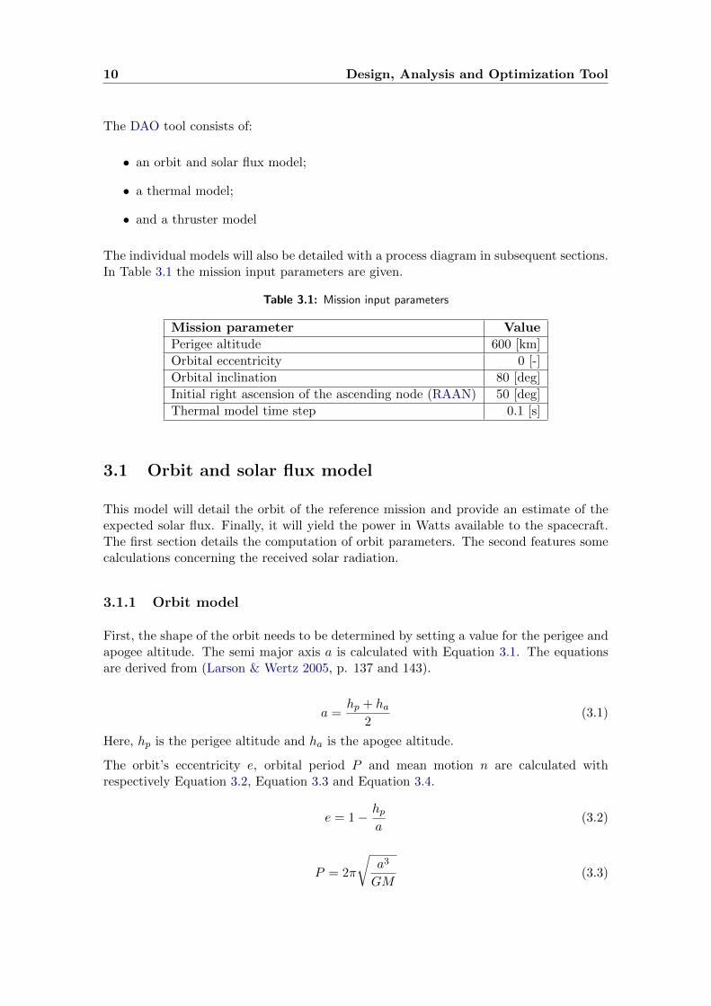
The DAO tool consists of:
• an orbit and solar flux model;
• a thermal model;
• and a thruster model
The individual models will also be detailed with a process diagram in subsequent sections.In Table 3.1 the mission input parameters are given.
Table 3.1: Mission input parameters
Mission parameter Value
Perigee altitude 600 [km]
Orbital eccentricity 0 [-]
Orbital inclination 80 [deg]
Initial right ascension of the ascending node (RAAN) 50 [deg]
Thermal model time step 0.1 [s]
3.1 Orbit and solar flux model
This model will detail the orbit of the reference mission and provide an estimate of theexpected solar flux. Finally, it will yield the power in Watts available to the spacecraft.The first section details the computation of orbit parameters. The second features somecalculations concerning the received solar radiation.
3.1.1 Orbit model
First, the shape of the orbit needs to be determined by setting a value for the perigee andapogee altitude. The semi major axis a is calculated with Equation 3.1. The equationsare derived from (Larson & Wertz 2005, p. 137 and 143).
a =hp + ha
2(3.1)
Here, hp is the perigee altitude and ha is the apogee altitude.
The orbit’s eccentricity e, orbital period P and mean motion n are calculated withrespectively Equation 3.2, Equation 3.3 and Equation 3.4.
e = 1− hpa
(3.2)
P = 2π
√a3
GM(3.3)

3.1 Orbit and solar flux model 11
n =
õ
a3(3.4)
Here, GM is the standard gravitational parameter of the parent body around which asatellite orbits. For Earth it is 398600.4418 km3s−2, for the Sun it is 132712.44·106 km3s−2.
Besides perigee, apogee and eccentricity, an orbit is also defined by the RAAN Ω and theinclination i. Due to the oblate shape of the Earth the gravitational attraction of theEarth is not homogeneous which causes a number of perturbations which in turn causethe precession of the RAAN. In Equation 3.5 this precession is calculated; the largestterm in the total perturbation is the J2-term and the computation therefore takes solelyits effect into account.
Ω = −1.5 · n · J2 · (REarth/a)2 · cos(i) · (1− e2)−2 (3.5)
Here, REarth is the radius of the Earth. The rate of change in RAAN Ω can be multipliedwith the time step and added to the initial RAAN angle to calculate the instantaneousRAAN during the mission.
A number of angles are required to compute the eclipse time. The applicable equationshave been taken from (Larson & Wertz 2005, p. 107). These include:
• δ, the sun’s declination angle with respect to Earth’s equator;
• βs, the angle of the Sun above the orbital plane;
• and Φorbit, the orbit’s rotation angle when the spacecraft is in eclipse.
The last two angles can be seen in Figure 3.2.
Figure 3.2: Orbit angles to determine solar flux Larson & Wertz (2005)

12 Design, Analysis and Optimization Tool
First, the δ-angle is computed with Equation 3.6. The d term in the equation indicatesthe number of days which have passed since the first of January in a particular day. Thesubtraction by 81 is to take into account the equinoxes when the declination angle is 0.
δ = arcsin ((sin(23.45) sin((360/365)(d− 81))) (3.6)
Second, the βs-angle is calculated with Equation 3.7. Note that Ω does not have to besubtracted with the Sun’s RAAN angle as both are determined based on the direction ofthe vernal equinox.
βs = arcsin(cos(δ) sin(i) sin(Ω) + sin(δ) cos(i)) (3.7)
Third, Φorbit is calculated in Equation 3.8.
Φorbit = 2 arccos
(cos(ρEarth)
cos(βs)
)(3.8)
Here ρEarth is the angular radius of the visible Earth disk as seen by the spacecraft.Equation 3.9 gives values for this variable.
ρEarth = arcsin(Re/hp) (3.9)
Finally, the eclipse time Pe is calculated in Equation 3.10.
Pe = P ·(
Φorbit
360
)(3.10)
3.1.2 Solar flux model
With the orbit model concluded, the solar flux is modelled in a simplified way. Thetrue anomaly θ indicates the angular position of Earth in its orbit with respect to theperihelion point on the 3rd of January. It is used to calculate an accurate estimate ofEarth’s instantaneous distance DSun−Earth to the Sun (Equation 3.11).
DSun−Earth =aEarth(1− e2Earth)
(1 + eEarthθ)(3.11)
Here, aEarth and eEarth are respectively the semi-major axis and eccentricity of Earth’sorbit. The solar flux in W/m2 is calculated with the equation below whilst using theinverse square law. Psun is the solar power output which is nearly constant at 3.856·1026
W.
S =Psun
4π(DSun−Earth · 1000)2(3.12)
The available power per hour Pa is calculated with Equation 3.13 where the orbital periodP is in seconds and the eclipse time Pe is in hours.
Pa = S · (P/3600− Pe) (3.13)

3.2 Thermal model 13
Looking at Figure 3.3 the available power indeed fluctuates slightly throughout the year.It indicates the radiation exposure over one year for a circular LEO orbit with an altitudeof 600 km, an inclination of 80 and a RAAN of 50. The power fluctuates over theyear from 1325 Whr/m2 to 1417 Whr/m2 with a mean at 1371 Whr/m2. In literaturethe mean solar flux or solar constant is indeed around 1371 Whr/m2 for LEO (Larson &Wertz 2005).
Figure 3.3: Plot for the available power and the eclipse time over one year for the referencemission
It is difficult to establish the fraction of incoming solar radiation or incoming solarpower which is reflected by the concentrator to the RAC. Ideally a prototype testingcampaign would be initiated and an average concentrator efficiency would be established.If one wants to determine an efficiency without tests, an average value has to be derivedfrom literature. In Nakamura et al. (2004) a concentrator efficiency of 70% to 90% wasestablished. Therefore a concentrator efficiency of 80% is assumed for the thermal model.
3.2 Thermal model
3.2.1 Introduction
The thermal model calculates the heat flow from the primary concentrator to the propellantand the power subsystem’s evaporator. In the introduction this heat transfer process wasalready shortly explained. To reiterate the following happens:
1. The primary concentrator radiates thermal energy to space and to the secondaryconcentrator; furthermore, it focuses solar radiation into the secondary concentrator.
2. The secondary concentrator radiates energy to space and to the cavity behind it; italso further focuses the solar radiation and conducts thermal energy to its casing.
14 Design, Analysis and Optimization Tool
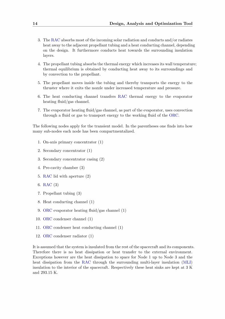
3. The RAC absorbs most of the incoming solar radiation and conducts and/or radiatesheat away to the adjacent propellant tubing and a heat conducting channel, dependingon the design. It furthermore conducts heat towards the surrounding insulationlayers.
4. The propellant tubing absorbs the thermal energy which increases its wall temperature;thermal equilibrium is obtained by conducting heat away to its surroundings andby convection to the propellant.
5. The propellant moves inside the tubing and thereby transports the energy to thethruster where it exits the nozzle under increased temperature and pressure.
6. The heat conducting channel transfers RAC thermal energy to the evaporatorheating fluid/gas channel.
7. The evaporator heating fluid/gas channel, as part of the evaporator, uses convectionthrough a fluid or gas to transport energy to the working fluid of the ORC.
The following nodes apply for the transient model. In the parentheses one finds into howmany sub-nodes each node has been compartmentalized.
1. On-axis primary concentrator (1)
2. Secondary concentrator (1)
3. Secondary concentrator casing (2)
4. Pre-cavity chamber (3)
5. RAC lid with aperture (2)
6. RAC (3)
7. Propellant tubing (3)
8. Heat conducting channel (1)
9. ORC evaporator heating fluid/gas channel (1)
10. ORC condenser channel (1)
11. ORC condenser heat conducting channel (1)
12. ORC condenser radiator (1)
It is assumed that the system is insulated from the rest of the spacecraft and its components.Therefore there is no heat dissipation or heat transfer to the external environment.Exceptions however are the heat dissipation to space for Node 1 up to Node 3 and theheat dissipation from the RAC through the surrounding multi-layer insulation (MLI)insulation to the interior of the spacecraft. Respectively these heat sinks are kept at 3 Kand 293.15 K.

3.2 Thermal model 15
The last three nodes are only used to calculate the architecture needed to replace thepower subsystem model’s active fluid-cooled condenser with a condenser with a passiveinterface with deep space (see Section 6.3.4).For Nodes 1 to 9 the thermal network is schematically depicted in Figure 3.4. TheRad, Cond and Conv depict respectively radiative, conductive and convective heat fluxes.Between Node 8 and Node 9 either a conductive or radiative interface can be realized.Both options are compared in terms of mass and size in Section 6.3.2.3.
Figure 3.4: Schematic of the thermal model node network
3.2.2 Geometries and properties of nodes
After the nodes have been established, the necessary geometries and properties have tobe determined.
16 Design, Analysis and Optimization Tool
3.2.2.1 Primary concentrator geometry and properties
First, the inflatable lens geometry for the primary concentrator is detailed. It consists oftwo polyimide-film membranes which form a lens and between which a pressure is appliedto inflate them. To form an inflatable lens, both a convex and a concave membrane haveto be fitted together. By assuming a value for the radius of curvature of the convexmembrane and the lens’ required focal length, the lens geometry can be calculated.First, in Equation 3.14 the relation between the curvature of both membranes is given.This equation is also known as the lensmaker’s equation Jenkins & White (1957).
f · ni = R1 −R2 +ni ·R1 ·R2
(ni − 1) · d(3.14)
Here f is the focal length, ni is the refraction index of the polyimide film, R1 is the radiusof the convex membrane and R2 is the radius of the concave membrane. Last, d is themaximum thickness of the lens.
The cross-sectional radius of the lens is also given. With the two radii of curvature andthe lens height, the back and frontal areas of the lens are calculated as both sides of thelens are treated as spherical caps. See Equation 3.15, 3.16 and 3.17 for more details. Thisequation also holds for the concave membrane.
θ1 = sin(Rcs/R1) (3.15)
h1 = R1(1− cos(θ1)) (3.16)
A1 = 2πR1h1 (3.17)
Figure 3.5 shows a graphical representation of the lens variables. Note that the lens area is
Figure 3.5: Representation of the concentrator lens variables
only important for calculating the radiating area to space. For receiving the solar energyonly the area perpendicular to the solar vector is used. This is simply a circular area witha radius equal to the primary concentrator cross-sectional radius.
The refraction index of Kapton polyimide is 1.70 and its thermal conductivity is 0.12W/mK (DuPont 2014). Its coating is a white paint with an emissivity of 0.9 and a solar

3.2 Thermal model 17
absorptance of 0.17 (AZ Technology 2008). Recall that in Section 3.1 a solar radiationthroughput efficiency of 80% was determined for the concentrator.
The secondary concentrator is modelled as a small parabolic lens in front of the RAC.Since the secondary concentrator lens is a thin lens, its lensmaker’s equation gets reducedfrom Equation 3.14 to Equation 3.18 (Jenkins & White 1957).
R1 =1
1R1
+ 1f · (
1n−1)
(3.18)
3.2.2.2 Secondary concentrator geometry and properties
The refractive secondary concentrator is assumed to be made of a single-crystal sapphirematerial. For such lenses an efficiency of 87% has been determined in solar vacuum tests(Wong et al. 2000). The emissivity of the single-crystal material is 0.02 and its highestthermal conductivity at 20 Celsius is 42 W/mK (Kyocera 2013).
The secondary concentrator casing is modelled as a thick disk around the secondaryconcentrator. In addition the thickness of the disk itself is assumed to be as long as thesum of the height of the concave and convex part of the secondary concentrator. Thewidth of the disk is the difference between the radius of the pre-cavity chamber and thecross-sectional radius of the secondary concentrator.The other cylindrical or spherical components in the solar thermal system assembly havea thickness based on literature and procurement data. Barlow’s equation is used to checkwhether the tubing thicknesses are sufficient for the tubing to cope with internal pressures(Equation 3.19).
ttubing =ptubingDouter−tubing
2σyield(3.19)
Here, ptubing is the fluid or gas pressure inside the tubing, Douter−tubing is the tubingouter diameter, σyield is the tubing material’s yield strength and ttubing is the tubing wallthickness.
3.2.2.3 RAC geometry and properties
The RAC can have different shapes. Different high conductive materials are available,such as tungsten, molybdenum and copper.The interior coating selection depends on its optical characteristics and the operatingtemperature range. It must have a high absorptance so that the RAC absorbs a lot ofsolar radiation. Gilmore (2002) has been used to select the coating for this part of thesystem. A carbon black paint coating is selected for the RAC. The coating’s absorptanceand emissivity are respectively 0.96 and 0.88.To limit the temperature of the secondary concentrator casing, a barium sulphate whitepaint coating is applied with an absorptance of 0.06 and an emissivity of 0.88. This allowsNode 3 to absorb as little direct sunlight as possible whilst emitting a large infrared (IR)
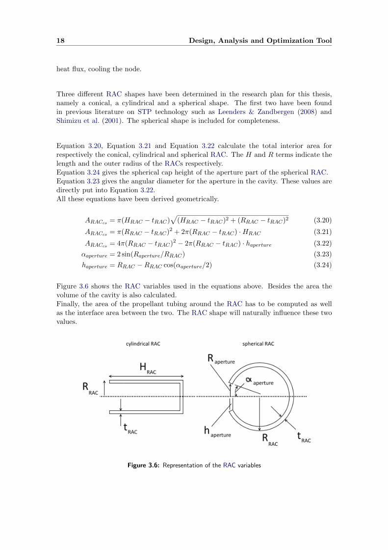
18 Design, Analysis and Optimization Tool
heat flux, cooling the node.
Three different RAC shapes have been determined in the research plan for this thesis,namely a conical, a cylindrical and a spherical shape. The first two have been foundin previous literature on STP technology such as Leenders & Zandbergen (2008) andShimizu et al. (2001). The spherical shape is included for completeness.
Equation 3.20, Equation 3.21 and Equation 3.22 calculate the total interior area forrespectively the conical, cylindrical and spherical RAC. The H and R terms indicate thelength and the outer radius of the RACs respectively.Equation 3.24 gives the spherical cap height of the aperture part of the spherical RAC.Equation 3.23 gives the angular diameter for the aperture in the cavity. These values aredirectly put into Equation 3.22.All these equations have been derived geometrically.
ARACcs = π(HRAC − tRAC)√
(HRAC − tRAC)2 + (RRAC − tRAC)2 (3.20)
ARACcs = π(RRAC − tRAC)2 + 2π(RRAC − tRAC) ·HRAC (3.21)
ARACcs = 4π(RRAC − tRAC)2 − 2π(RRAC − tRAC) · haperture (3.22)
αaperture = 2 sin(Raperture/RRAC) (3.23)
haperture = RRAC −RRAC cos(αaperture/2) (3.24)
Figure 3.6 shows the RAC variables used in the equations above. Besides the area thevolume of the cavity is also calculated.Finally, the area of the propellant tubing around the RAC has to be computed as wellas the interface area between the two. The RAC shape will naturally influence these twovalues.
Figure 3.6: Representation of the RAC variables

3.2 Thermal model 19
3.2.3 Tubing configurations
Besides the absorber, the tubing configuration has to be detailed for the conical, cylindricaland spherical cavities respectively. First, the spiral configuration will be examined;afterwards the linear configuration will be discussed.
3.2.3.1 Spiral tubing configuration
The spiral arc length can be detailed with the help of three parametric equations. Perconfiguration respectively this set of three equations is given in Equation 3.25, Equation3.26 and Equation 3.27. The parametric equations have been applied of respectively aconical spiral, a helix and a spherical spiral.
x = a cos(θlocal) (3.25a)
y = a sin(θlocal) (3.25b)
z = c · θlocal (3.25c)
a =tan(δcone) · Ptubing
(2π · θlocal)(3.25d)
c =Ptubing
2π(3.25e)
x = a cos(θlocal) (3.26a)
y = a sin(θlocal) (3.26b)
z = c · θlocal (3.26c)
a = Rpath (3.26d)
c =Ptubing
2π(3.26e)
x =Rpath cos(θlocal)(√c2 · θ2local + 1
) (3.27a)
y =Rpath sin(θlocal)(√c2 · θ2local + 1
) (3.27b)

20 Design, Analysis and Optimization Tool
z =−c ·Rpathθlocal(√c2 · θ2local + 1
) (3.27c)
c =Ptubing
2π(3.27d)
In the equations above, Rpath is the maximum radius of the spiral tubing’s path andPtubing is the pitch of the spiral tubing which is the distance between each turn of thespiral.Figure 3.7 shows the variables for spiral tubing around a hypothetical cylindrical RAC.
Figure 3.7: Representation of the spiral tubing variables
Finally, each parametric equation is differentiated with respect to θlocal, which yields x′,y′ and z′. These terms are squared, summed up and combined in a finite integral whichis solved along the interval of [0 : 2π · nturns] where nturns are the total number of turnsin the spiral (Equation 3.28).
Ltubing = 0.92 ·∫ [2π·nturns]
0
√x′2 + y′2 + z′2 (3.28)
The final interface area is calculated by multiplying Ltubing with the width of the interfacearea between the RAC and tubing. A 25% margin is taken from one third of the tubinglength to account for a decrease of the practical length due to geometrical constraints atthe rear side of the RAC. This translates to about an 8% decrease of the total length.
3.2.3.2 Linear tubing configuration
Now the linear tubing geometric characteristics are discussed. Equation 3.29 to 3.31calculate all three RAC tubing lengths. As with the spiral tubing, a margin is taken offthe tubing length of the third tubing part to take into account the loss of tubing due togeometrical constraints. Since straight tubing is less challenging in terms of integration,

3.2 Thermal model 21
only a margin of 10% is assumed. This translates to around a 3% decrease of the totallength.
Ltubing = 0.97√R2path +H2
RAC (3.29)
Ltubing = 0.97HRAC (3.30)
Ltubing = 0.97πRpath (3.31)
The number of linear propellant feed lines is only taken into account when computingthe final propellant temperature, as the convection area increases with more propellanttubing along the RAC.
3.2.4 Heat conducting channel and evaporator
The heat conducting channel interfaces with the RAC and the evaporator heating fluid/gaschannel. It is modelled as a solid rod emanating radially from the RAC with a predeterminedlength.The total contact surfaces between the RAC and the conduits and the conduits andthe evaporator are a multiplication of the number of channels with their individualcross-sectional areas.
3.2.5 View factors
The view factors will partly determine the amount of thermal energy which is radiatedbetween the nodes. Bergman et al. (2011) has been consulted for the necessary equations.Before one can start with calculating the view factors two relations must be put forward.
ΣF = 1 (3.32a)
A1 · F12 = A2 · F21 (3.32b)
Equation 3.32 states that the sum of all view factors from one node to the others must be1. It also says that the product of the view factor of one node to another and the area ofthe first node must equal the product of the reciprocal terms concerning the second node.
Note that the secondary concentrator casing and the cavity lid are considered insulatedat their sides. Therefore, the sides of these components are not taken into accountwhen computing view factors. For the computation of the view factors one is referred toAppendix A.One should also note that the assumption is made for all cavity configurations that thereis no radiative heat exchange between node 2 and node 6, since re-radiation is limiteddue to the presence of the cavity lid.Last, the spherical RAC’s view factors are calculated with the assumption that the viewfactor between Node 5 and the interior of Node 6 is zero as calculating this view factor isconsidered too complex and time consuming without more advanced software.
22 Design, Analysis and Optimization Tool
3.2.6 Gebhart factors and thermal couplings
Gebhart factors indicate the ratio of absorbed radiation by a surface over the totalradiation emitted by the principal surface. These factors are necessary to calculateradiative heat transfer. As with the view factors, the sum of all Gebhart factors from anysurface must be 1. Since the view factors have been preliminarily calculated, the sum foreach node might not amount to exactly 1. As this is a feasibility study, this is deemedacceptable.In addition, Equation 3.33 applies. The Gebhart factors themselves can be computedwith Equation 3.34 (Bergman et al. 2011).
εiAiBij = εjAjBji = Rij = Rji (3.33)
Bij = Fijεj (3.34)
Here Bij is the Gebhart factor. The variable ε is the emissivity of the surface and Rij isthe radiative coupling between thermal nodes.The effect of reflections from other neighbouring surfaces needs to be taken into accountin case of an enclosed surface. Equation 3.35 Bergman et al. (2011) shows this.
Bij = Bij + ψ · FikBkj (3.35)
Here ψ is the reflectivity factor which is (1 − ε). The subscript k indicates adjacent orfacing surfaces other than node i or node j. The equation is applied for Node 2 up toNode 5 as the pre-cavity chamber (Node 4) and its adjacent nodes can be considered avirtually closed section.
With the Gebhart factors known the radiative couplings can be calculated. Besidesradiative couplings one can also discern conductive couplings which represent conductionprocesses between nodes. These can be calculated with Equation 3.36 (Bergman et al.2011).
Cij =ki ·AicsLi
(3.36)
Here, Cij is the conductive coupling, ki is the thermal conductivity of the node’s material,Aics is the cross-sectional area of the node and Li is the conductive path length betweennodes.Note that conductance between the primary concentrator and its struts or other componentsis assumed negligible.
The radiative and conductive heat fluxes are calculated with equations 3.37 and 3.38(Bergman et al. 2011).
Qijrad = Rijσ(T 4i − T 4
j ) (3.37)
Qijcond = Cij(Ti − Tj) (3.38)

3.2 Thermal model 23
3.2.7 Convective heat flow
Finally, the convective heat transfer from the propellant tubing inner wall to the propellantis discussed.First, the convective heat transfer coefficient must be calculated. To this end Cornelisseet al. (1979) provides Equation 3.39.
hc =Nu · k
Dinner−tubing(3.39)
The coefficient is hc. The Nu parameter is the Nusselt number and Dinner−tubing is thepropellant tubing inner diameter.
3.2.7.1 Nusselt, Prandtl and Reynolds numbers
The Nusselt number is calculated with Equation 3.40. This Sieder-Tate correlation takesinto account the viscosity variations in the propellant, assuming turbulent gaseous flowas detailed in Sieder & Tate (1936).
Nu = 1.86(Re · Pr)(1/3)(Douter−tubingLtubing
)(1/3)(µpropfree−streamµpropwall
)0.14
(3.40)
Here, Pr is the Prandtl number, Re is the Reynolds number and µprop is the propellantflow viscosity, here in two different locations and computed through Equation 3.45.Equation 3.41 calculates the Prandtl number (Bergman et al. 2011).
Pr =cspecificpropµprop
k(3.41)
The specific heat capacity of the propellant is denoted by cspecificprop . The Reynoldsnumber is calculated with Equation 3.42 (Bergman et al. 2011).
Re =ρpropUpropDinner−tubing
µprop(3.42)
The propellant flow density is denoted by ρprop; Uprop is the propellant flow velocity.
3.2.8 Flow properties in tubing
The flow velocity, viscosity and density in the tubing are calculated according to theequations below and fed into Equation 3.42.
ρprop =(pchamber + δp)
RgasTpropinitial(3.43)
Here, pchamber is the thruster chamber pressure, δp is the pressure loss in the tubingand Rgas is the specific gas constant. The equation is an expression of the ideal gas law(Bergman et al. 2011).

24 Design, Analysis and Optimization Tool
The flow velocity in the tubing is calculated with Equation 3.44 according to the law ofconservation of mass (Bergman et al. 2011).
Uprop =mprop
ρpropAtubingcs(3.44)
In this equation mprop is the mass flow through the tubing and Atubingcs is the innercross-sectional area of the RAC-adjacent propellant tubing.
The flow viscosity is calculated using Sutherland’s equation (Equation 3.45) (Sutherland1893).
µprop = µprop0 ·273.15 + CSutherland
(Tf/273.15)(3/2)(3.45)
Here, µprop0 is the propellant viscosity at 273.15 K, Tf is the average propellant filmtemperature and CSutherland is the Sutherland constant which is unique for every propellant.
The film temperature is an average between the wall temperature and the propellanttemperature. Since the propellant temperature varies along the length of the propellanttubing, the propellant temperature in question is itself an average of the final and initialtemperature.
3.2.9 Temperature calculations
The energy flux associated with the convection processes in the propellant tubing (Node7) and the evaporator heting fluid/gas channel (Node 9) is calculated in Equation 3.46.As previously, Bergman et al. (2011) has been consulted for the applicable equations.
Qconv = mpropcspecificprop(Tpropfinal − Tpropinitial) (3.46)
As one can see the convective heat transfer is multiplied with the mass flow and thespecific heat capacity of the propellant as well as with the difference between initial andfinal propellant temperature. The final propellant temperature is calculated in Equation3.48.The initial propellant temperature Tprop,initial is already defined. The initial mean propellanttemperature Tm can therefore be calculated.
Tminitial =Tpropinitial + Tinner−tubingwall
2(3.47)
Tpropfinal = Tpropinitial + hc(Tinner−tubingwall − Tm)Ainner−tubingcs
mpropcspecificprop(3.48)
Tmnew =Tpropinitial + Tpropfinal
2
In the case that latent heat needs to be put into the propellant to change its phaseEquation 3.48 becomes Equation 3.49.
Tpropfinal = Tpropinitial + hc(Tinner−tubingwall − Tm)Ainner−tubingcs
mpropcspecificprop− qlatentcspecificprop
(3.49)

3.2 Thermal model 25
Here, qlatent is the latent heat required to vaporize the selected propellant.
These equations are used in an iterative process where for each time instance the valuesare recalculated. Note that Tminitial is only valid up until the point that the propellantstarts flowing. Afterwards Tmnew takes its place since it is more accurate than the formervariable. The final propellant temperature is subsequently calculated and plotted for eachtime instance. The maximum value in the array of final propellant temperatures is usedin the same iterative scheme for performing calculations in the thruster model. At thestart of the iterative cycle however an arbitrary value for the final propellant temperaturewill be put into the thruster calculations.
In addition these equations are used when calculating the heat flux from the ORC workingfluid via the passive condenser to space.The applicable heat flux equations for the passive condenser are as follows.
∆Qcondenser = Qconv − Ccond1 −Qradint (3.50)
∆Qconductor = Ccond1 − Ccond2 (3.51)
∆Qradiator = Qradint + Ccond2 −Qradext (3.52)
Qconvection = mwfcspecific(Twfinitial − Twffinal) (3.53)
Qradext = εσAradiatorT4radiator (3.54)
The ext and int subscripts indicate whether the flux comes from inside or outside thesystem. The cond subscripts indicate first the conduction between condenser and conductorchannel and second between conductor channel and the radiator. The radiator has anarea Aradiator and a temperature Tradiator. The rad subscript indicates a radiative heatflux.The internal radiative heat flux occurs between the condenser outer wall and the radiatorpanel interior. The external radiative heat flux occurs from the radiator exterior to space.If conductive heat exchange is selected for the heat transfer between condenser andradiator Qradint becomes zero. If radiative heat exchange is selected ∆Qconductor andthe Ccond terms become zero.
As the model is transient, the heat fluxes are dependent on time, as is seen in Equation3.55. Here, the change in flux for each node has been computed (Equation 3.56).
Ti(t) = Ti(t− 1) +∆Qi(t)
Micspecifici∆t (3.55)
Here ∆Qi is the net heat flux into node i. It is computed according to Equation 3.56.
∆Qi(t) = Qiext + ΣQinint − ΣQoutint (3.56)
Also the variable Mi indicates the mass of the thermal node. The mass for each nodeis calculated by multiplying the frontal surface areas by the representative thickness andmultiplying this value by the material’s density. Alternatively, the density is multipliedwith the node’s volume.

26 Design, Analysis and Optimization Tool
The time step is denoted by ∆t. This calculation is made for every node at every time twhich is incremented by time step ∆t after every calculation. The temperature T (t− 1)at the previous time instance is taken from previous calculations with a pre-defined initialvalue at t = 0.
The external flux terms previously defined as Qiext are calculated with Equations 3.57 to3.61.
Q1ext = α1AprimcsS (3.57)
Q2ext = α2AprimcsSηprim (3.58)
Q6ext = α2AprimcsSηprimηsec (3.59)
Qalbedo = 0.3S ·Aαnode (3.60)
QIR = 244 ·Aεnode (3.61)
Here, α is the solar absorptance of the node, ε is the IR emissivity of the node, Aprimcs isthe cross-sectional area of the primary concentrator facing the Sun and S is the solar flux.The η-terms are the (throughput) efficiency of the primary and secondary concentrator.In Section 3.2.2 values for these efficiencies were respectively identified at 0.80 and at0.87.
The last two equations are respectively the albedo radiation and the average IR radiationwhich are both emitted by the Earth and received by Node 1 to Node 3. Note that ineclipse there is no sunlight and therefore also no albedo.
Note that the propellant flow is only initialized after the cavity has reached a certaintemperature. This ’propellant flow initialization cavity temperature’ can be varied accordingto the necessary performance of the system. The model assumes that during propellantflow solar radiation will constantly be focused towards the cavity. In addition the initialpropellant temperature is assumed to be the propellant storage temperature.
The thermal model process is illustrated by the process diagram in Figure 3.8. The mainiterative cycle occurs when the thermal node temperatures and the accompanying meanheating gas temperature are calculated. This also involves iterations of the ORCHID-VPEmodel which details the thermodynamic processes in the power subsystem. Afterwardsthe final and mean propellant temperatures are calculated and put in the output dataarray. More details about the ORCHID-VPE model are given in Section 4.1.
3.2.10 Pressure losses
The pressure losses in the tubing need to be calculated to estimate the pressure in thepropellant feed system. Equation 3.62 computes the single-phase friction pressure losses.Equation 3.66 deals with the pressure losses due to the phase change in the first partof the RAC tubing. Equation 3.67 calculates the acceleration pressure loss due to thevaporization of the propellant.

3.2 Thermal model 27
Figure 3.8: Process diagram for thermal model
3.2.10.1 Single-phase flow friction pressure loss
The Darcy-Weisbach equation is used to calculate the single-phase friction pressure loss.
δpfrictionsingle−phase = fDL
D
ρV 2
2(3.62)
The term fD is the Darcy friction factor associated with the nature of the flow. It iscalculated with the Blasius equation (Equation 3.63). This is assuming smooth propellanttubes. The L and D terms are respectively the length and inner diameter of the tubingin question. The ρ and V variables are the density and velocity of the propellant in thetubing.
fD =0.316
Re0.25(3.63)

28 Design, Analysis and Optimization Tool
3.2.10.2 Two-phase flow friction pressure loss
McKetta Jr. (1992) offers a method to estimate pressure losses due to the existence oftwo phases within a pipe. The two-phase flow patterns within a pipe can be identifiedbased on Baker parameters. These parameters are Bx and By. Equation 3.64 and 3.65are used to compute them.
Bx = 2.1039Wl
Wv
√ρlρv
ρ(2/3)l
µ(1/3)l
σl(3.64)
By =25524.62Wv(A√ρlρv
) (3.65)
Here, W is the flow rate and ρ is the density of the propellant. The liquid phase viscosityand the liquid phase surface tension are represented by µl and σl. The terms at thefront of the equations are scaling factors to take into account metric units as the originalequations use imperial units. The subscripts l and v indicate respectively that one isdealing with the liquid and gaseous properties of the propellant.Looking at Figure 3.9 and taking the intersection of the calculated Baker parameters, aparticular two-phase flow regime can be identified.
Figure 3.9: Two-phase flow region identification (McKetta Jr. 1992)
Depending on the region a different unit loss correlation is selected. The unit loss φ isused in Equation 3.66 to calculate the pressure loss. Here, the pressure loss of the gaseousstate δpv is calculated with Equation 3.62 along the length where the two-phase mixtureexists.
δpfrictiontwo−phase = δpv · φ2 (3.66)
3.3 Thruster Model 29
3.2.10.3 Acceleration pressure loss
The acceleration pressure loss originates from the acceleration of the propellant flow dueto vaporization of the liquid propellant. Fang et al. (2012) gives Equation 3.67 which isa derived equation for this pressure loss.
δpacceleration =(mA
)2( 1
ρout− 1
ρin
)(3.67)
The in and out subscripts indicate the in- or outlet flow conditions. The total pressureloss is then determined by summing up the different pressure losses.
δptotal = δpfrictiontotal + δpacceleration (3.68)
In Chapter 6 these pressure losses will be calculated when designing the detailed propellantfeed system.
3.3 Thruster Model
3.3.1 Introduction
The thruster model produces a first estimate of thruster performance in terms of specificimpulse, thrust and propellant mass. The input variables are chamber conditions such aspressure, propellant density and temperature. Viscosity, specific heats ratio and specificgas constant are dependent on the propellant choice. Nozzle shape variables such asexpansion ratio round up the input variables.
3.3.2 Nozzle shape
The nozzle shape depends on whether a conical or bell-shape nozzle is selected. The basicnozzle shape however is always the same (Figure 3.10):
• A convergent segment
• A curved convergent region towards the throat
• The throat with constant cross-sectional area
• A curved divergent region away from the throat
• A divergent segment with linearly or non-linearly increasing cross-sectional area
The assumption is made that the chamber radius equals the maximum radius of theconvergent section. The throat radius is a set fraction of the maximum radius. Theexhaust radius Rexhaust determined by taking the squared root of the expansion ratio andmultiplying this by the throat radius. In Equations 3.69 and 3.70 the x- and y-coordinate

30 Design, Analysis and Optimization Tool
Figure 3.10: Representation of nozzle shape
of the start of the curved convergent region is calculated in order to plot the shape of thenozzle using basic geometrical relations.
xcurved = Rcurved sin(θconvergence) (3.69)
ycurved = Rthroat +Rcurved (1− cos(θconvergence)) (3.70)
Here, Rthroat is the throat radius, Rcurved is the radius of the curved convergent sectionand θconvergence is the nozzle convergent half angle. Figure 3.10 shows these variables.The same procedure is used for the divergent curved section. The length from the start ofthe nozzle to the throat is added, after the x-coordinate has been calculated, to providea consistent nozzle x-axis.
3.3.2.1 Conical nozzle
The conical nozzle shape is finished by using the nozzle exhaust radius to define thelength of the divergent segment as the latter is dependent on the former and the nozzledivergence half angle. The nozzle divergence half angle θdivergence denotes the slope of thedivergent segment. The y-coordinate is therefore dependent on the x-coordinate as seenin Equation 3.71
y = ycurved + tan(θdivergence · (x− xcurved) (3.71)
3.3.2.2 Bell-shaped nozzle
The bell-shaped nozzle requires a parametric expression for a parabola to estimate the bellshape of the nozzle. Three coefficients first need to be determined. They are dependent onθexhaust which is the nozzle exhaust divergence half angle or the angle which the nozzle hasat the exhaust with respect to the horizontal. Equation 3.72 to 3.74 show the expressionsfor the coefficients.Equation 3.75 gives the calculation for the x coordinate of the exhaust. By taking anumber of values for xnozzle and solving Equation 3.76 for ynozzle the y-coordinates of the

3.3 Thruster Model 31
divergent segment of the bell-shaped nozzle can be determined.
a =(tan (π/2− θexhaust)− tan (pi/2− θexhaust))
2(Rexhaust − ycurved)(3.72)
b = tan (π/2− θdivergence)−
2(tan (π/2− θexhaust)− tan (pi/2− θexhaust))
2(Rexhaust − ycurved)· ycurved (3.73)
c = xcurved − a · y2curved − b · ycurved (3.74)
xexhaust = a ·R2exhaust + b ·Rexhaust + c (3.75)
xnozzle = a · y2nozzle + b · ynozzle + c (3.76)
3.3.3 Nozzle critical flow conditions
In order to design an optimal nozzle the critical conditions need to be known in thethroat so that the flow achieves sonic conditions exactly at the throat. This will preventshocks and severe pressure drops in the nozzle. The subscript critical denotes the criticalconditions in the throat. The subscript chamber specifies thruster chamber conditions.Equation 3.77 to Equation 3.81 calculate respectively the local pressure, local density,temperature, mass flow and flow velocity in the throat under sonic conditions (Anderson2010).
pcritical = pchamber
(2
γprop + 1
)(γpropγprop−1
)(3.77)
ρcritical = ρchamberpcriticalpchamber
(1/γprop)(3.78)
Tcritical = Tchamber2
γprop + 1(3.79)
mcritical = pchamberΦπR2
throat√RgasTchamber
(3.80)
Ucritical =√γpropRTcritical (3.81)
(3.82)
The variable γprop is the specific heats ratio of the selected propellant. Tcritical is thecritical propellant flow temperature. Tchamber is the propellant temperature in the thrusterchamber. The assumption is made that between the end of the propellant tubing adjacentthe RAC and the thruster chamber the propellant temperature decreases by 5% due toheat dissipation out of the tubing. The variable mcritical is the critical mass flow in thethroat. Φ is the Vandenkerckhove function and Rgas is the specific gas constant.Finally, the throat flow velocity Ucritical can be calculated.

32 Design, Analysis and Optimization Tool
3.3.4 Chamber flow conditions
The ideal flow velocity in the chamber is calculated with the following equation (Anderson2010). The resulting Uchamber is usually significantly smaller than Ucritical.
Uchamber =ρcriticalAthroatUcriticalρchamberAchamber
(3.83)
The corresponding Mach number is achieved through Equation 3.84 (Anderson 2010).These values can also be calculated all along the nozzle length.
Machamber =Uchamber√
γpropRTchamber(3.84)
In this equation Ma is the Mach number. If the calculations of the flow velocity and Machnumber are successfully executed, one will observe a Mach number of 1 at the throat.
3.3.5 Thruster and propulsion subsystem performance
Once the propellant flow in the nozzle has been determined, the equivalent or effectiveexhaust velocity Ueq can be calculated with Equation 3.85 (Sutton & Biblarz 2001). Notethat the ambient pressure pa outside of the nozzle in this case is 0 bar as one operates ina vacuum. The pressure at the exhaust is pe.
Ueq = Uexhaust +(pe − pa)Aexhaust
mexhaust(3.85)
The specific impulse Isp is calculated through Equation 3.86 (Sutton & Biblarz 2001).
Isp =Ueqg0
(3.86)
The parameter g0 is the standard gravitational acceleration which is 9.81 m/s2.Before the resulting thrust is calculated, thrust losses due to flow divergence and the
presence of a boundary layer need to be taken into account. The first component iscomputed with Equation 3.87 and 3.88 for respectively a conical and bell-shaped nozzle(Berton 1991), the second with Equation 3.91.
cthrust−loss =1 + cos(θdivergence)
2(3.87)
Note that cthrust−loss is a fraction of the total thrust.
For a bell-shaped nozzle correlation data is present, although an equation is unavailable.Therefore an equation is devised by subtracting the nozzle exhaust divergence half anglefrom the nozzle divergence half angle in Equation 3.87. An additional correction factor of0.99 is put in to match actual correction factors for bell-shaped nozzles (Sutton & Biblarz2001, p. 81). This yields Equation 3.88.
cthrust−loss = 0.991 + cos(θdivergence − θexhaust)
2(3.88)

3.3 Thruster Model 33
The boundary layer thrust loss is calculated as follows. Equation 3.89 calculates themomentum thickness due to the presence of a boundary layer (Schlichting & Gersten2000, p. 161). Equation 3.90 uses this value to calculate the resulting thrust loss per unitspan (Tennekes & Lumley 1972, p. 112). Multiplying by the nozzle edge length, which is2πRexhaust, gives the thrust loss estimate as shown in Equation 3.91.
θmomentum = 0.664 ·√µpropxbl
Uexhaust(3.89)
δTlossblδx
= θmomentumρexhaustU2exhaust (3.90)
Tlossbl = θmomentumρexhaustU2exhaust · 2πRexhaust (3.91)
Here, θmomentum is the momentum thickness as a function of edge length and the thrustloss is an absolute value in Newton. The xbl variable specifies the distance downstreamfrom the throat where the boundary layer develops along the nozzle wall. In this case adistance of one third of the total divergent nozzle length is assumed.The final thrust Tthrust is computed, using Equation 3.92 (Sutton & Biblarz 2001).
Tthrust = cthrust−lossmexhaustUexhaust + (pe − pa)Aexhaust − Tlossbl (3.92)
Note that the thrust takes into account the thrust due to output mass flow as well asthe thrust due to the pressure differential between the exhaust pressure and the spacevacuum. The boundary layer thrust loss is calculated and can be considered negligiblefor these small nozzles.
The required propellant mass is calculated by solving Equation 3.93 which is Tsjolkovski’srocket equation.
∆Vrequired = Ueq log
(Md +Mprop
Md
)(3.93)
The Md is the spacecraft dry mass and Mprop is the total propellant mass stored within thespacecraft. A 20% residual propellant margin is added on top of the required propellantmass to take into account inaccuracies and possible attitude determination and controlsystem (ADCS) use of the propellant.The thrust time, total impulse and system-specific impulse are respectively calculatedwith Equation 3.94, 3.95 and 3.96 (Sutton & Biblarz 2001). The variable Mwet is the wetpropulsion subsystem mass.
tthrust =Mp
mp(3.94)
Itotal = Tthrusttthrust (3.95)
Issp =Itotalg0Mwet
(3.96)
Figure 3.11 details the process in the thruster model.

34 Design, Analysis and Optimization Tool
Figure 3.11: Process diagram for thruster model
3.4 Verification and validation
As one is dealing with mathematical models verification and validation need to be performedto detect faults.
Verification was first performed by varying design variables and seeing whether thrust,system mass and component temperatures increased or decreased as expected. Furthermorearbitrary design variables were selected to see whether performance values were in theorder of magnitude as defined in Leenders & Zandbergen (2008), Shimizu et al. (2001),Nakamura et al. (2004), Sahara & Shimizu (2003) and Sahara et al. (2000). These includeabsorber temperatures in the range 1000-3000 K, thrust levels from 0.1-1 N and specificimpulses of 700-900 s for hydrogen propellants. The absorber sizes which have been usedduring verification are in the range of 4 mm to 25 mm as derived from the previouslyidentified literature.
After successful verification, the model was validated using test results from literature.First, the variables with regard to the thruster were validated as detailed in Subsection3.4.1. Subsection 3.4.2 features the validation results in terms of final propellant and RACtemperatures. Because of the scarcity of test data only a qualitative validation could bepursued. A quantitative validation will have to be performed in the future once an actualsystem has been built.

3.4 Verification and validation 35
3.4.1 Thrust, specific impulse and mass flow validation
First, the properties from the DUT solar thermal thruster as developed and reported byLeenders & Zandbergen (2008) are applied to the model.The thruster is a conical copper thruster which is provided with gaseous nitrogen propellantto generate thrust. The propellant feed lines along the RAC are linear and integratedinto the absorber wall. The nozzle itself is a micro nozzle.Tests with and without propellant flow were performed with the former being the mostinteresting in this case. The highest stable propellant temperature achieved was 525 K ata mass flow of 50 mg/s. When increasing the mass flow, the thrust and pressure increasedwhereas the propellant and cavity temperature decreased. Thrust levels of 29 to 81 mNwere measured.Figure 3.12 provides a temperature profile for one of the tests.
Figure 3.12: Leenders & Zandbergen (2008) test results
The input variables and their values for the validation have been given in Table 3.2. Notethat the evaporator conducting channel and heating fluid/gas channel have not beenincluded whilst running the model. Also the 10% margin decrease of part of the lineartubing length has been omitted. Furthermore the outside secondary concentrator casingis assumed made of molybdenum with a white paint coating. The cavity and propellanttubing are assumed made of copper. The pre-cavity and apertured cavity cover have MLIradiative properties.
The model is run. This yields the following results. First, a thrust of 100.6 mN iscalculated. The specific impulse is 71.3 s. The mass flow at the exhaust is 104 mg/s.For the 2-bar inlet pressure the test results give a mass flow of 77 mg/s and a thrust of28.9 mN.
Although the results in Table 3.3 do not correspond exactly, they are within the sameorder of magnitude. This is considered acceptable, since the exact configuration of theDUT propulsion system is unknown, except for a small number of design variables.In addition ideal thruster performance has been assumed and thrust losses have been

36 Design, Analysis and Optimization Tool
Table 3.2: Model input variables for validation (Leenders & Zandbergen 2008)
Model variable Value
Cross-sectional radius of primary concentrator 0.05 [m]
Radius of curvature for the primary concentrator convex membrane 0.125 [m]
Concentration ratio for primary concentrator 1/0.23 [-]
Primary concentrator focal length 0.01 [m]
Concentration ratio for secondary concentrator 1
Secondary concentrator focal length 0.01 [m]
Thickness of primary concentrator along lens axis 0.005 [m]
Cavity maximum radius 0.0125 [m]
Cavity length 0.0501 [m]
Chamber radius 0.0015 [m]
Chamber pressure 2 [bar]
Throat radius 0.00029 [m]
Length of divergent section 0.001 [m]
Expansion ratio 1.375 [-]
Number of lines for the linear propellant tubing 8 [-]
Diameter of the propellant tubing 6.77E-4 [m]
Type of RAC Conical
RAC material Copper
RAC wall thickness 2.5 [mm]
Type of tubing Linear
Type of divergent nozzle Conical
Type of propellant Nitrogen
Propellant flow initialization cavity temperature 650 [K]
Solar flux 2350 [W/m2]
Conducting interface (between RAC and tubing) width 4.84E-5 [m]
Table 3.3: Comparison of model and test performance
Performancevariable
Model Test results (Leenders & Zandbergen2008)
Thrust [mN] 100.6 28.9
Specific impulse [s] 71.3 38.2
Mass flow [mg/s] 104 77
neglected whereas this will not be the case during real-life tests. Finally, one shouldexpect a higher mass flow to produce a higher specific impulse and thrust which is indeedthe case for the model. The thruster model is therefore qualitatively validated.
3.4.2 Temperature validation
The concept by Leenders & Zandbergen (2008) is used once more for the validationof model temperatures. Specifically, the final cavity and propellant temperatures arechecked. The Shimizu et al. (2001) concept literature is deemed unsuitable to provideenough design variables. In this case the concept can therefore not be used to conduct areliable validation.
Although the STP system as described by the model is different than the system design

3.4 Verification and validation 37
of the DUT reference concept, care is taken to approximate the design as best as possible.First, a propellant flow initialization cavity temperature of 650 K is assumed. One seventhof the outer propellant tubing radius is assumed to be the width of the conducting interfacebetween the tubing and the RAC.Constant mass flow is assumed. Furthermore a power input into the system of 2350 W/m2
is applied as specified.In terms of materials the cavity lid is made of MLI material to simulate surroundinginsulation; the cavity and the propellant tubing are made of copper.Furthermore a certain heat dissipation from the RAC to the external environment hasbeen assumed. This heat flux has been modelled as a conductive heat flux to a MLIblanket surrounding the areas of the cavity which do not have adjacent tubing. Thislayer has twice the thickness of the RAC and a thermal conductivity of 0.24 W/mK. TheMLI-layer is kept at a room-temperature of 293.15 K. The input variables are given inTable 3.2.
Finally, an instantaneous propellant flow initialization is assumed. This causes an initialspike in the propellant temperature which is unrepresentative of real-life conditions wherethe propellant flow increases over a short period to a steady flow.In Figure 3.13 one can take a closer look at the resulting instability in the propellanttemperature plot during a model validation run. In the 14th minute into the simulationa spike can be seen which drops down almost instantly after which the curve continues ina normal manner.
Figure 3.13: Instability of the initial propellant temperature values
To remove the instability from the results, the propellant flow temperatures during thefirst 11 to 30 seconds after flow initialization have been removed from subsequent plots.The simulated temperatures of the thermal nodes can be seen in Figure 3.14.
Comparing Figure 3.12 and Figure 3.14, the time till the cavity reaches 650 K is also

38 Design, Analysis and Optimization Tool
Figure 3.14: Temperatures for the DUT concept as modelled by the DAO tool
Table 3.4: Comparison of model and test temperatures
Temperature Model Test results (Leenders &Zandbergen 2008)
Maximum cavitytemperature
652 650
Final cavitytemperature
522 525
Maximum propellanttemperature
489 525
Final steady propellanttemperature
420 477
approximately 20 minutes for the model. The discrepancies in Table 3.4 stem from theassumed thermal uniformity of the thermal nodes, the limited number of thermal nodes,differences in mass flow in the feed lines and the non-constant propellant flow duringactual testing. Furthermore, in the model the propellant tubing is not incorporated intothe cavity whereas this is the case in the DUT design. One would therefore expect alarger convective area, a larger heat flux into the propellant and hence a larger propellanttemperature. Adding more heat flux exchange processes between the different nodes andincreasing the number of nodes will produce a more equivalent result, but will lead to anincrease in the runtime of the simulation.

3.5 Observations 39
Furthermore, when varying the inlet pressure of the thruster the same relative ratios ofmass flow are achieved. During the DUT thruster tests the mass flow increases from 77 to128 mg/s when increasing the pressure from 2 to 3 bar. In the model the same simulatedmass flow increases from 104 to 163 mg/s. This represents respectively a ratio of 0.60and 0.64.All these observations considered, the thermal model is qualitatively validated.
3.5 Observations
After running the model and changing different design variables, some observations canbe made concerning the effect of design changes on the system’s performance. Thefollowing design variables remain unchanged. The secondary concentrator casing is madeof molybdenum with a white paint coating. All the other nodes are made of non-coatedmolybdenum, except for the cavity which has a black coating for a high solar absorptance.The propellant flow initialization cavity temperature is 1600 K.Note that the figures in this section depict temperature profiles for a conical RAC. Theseresults can however be extrapolated to other configurations.
3.5.1 Increasing convection area
Increasing the number of spiral turns increases the final propellant temperature. Thismakes sense as an increased number of turns leads to an increased length of the propellanttubing and consequently a larger convective area. One can indeed see that if in Equation3.48 Ainner−tubingcs increases the final propellant temperature will increase. Looking atFigure 3.15 also shows an increase when the number of turns is increased from 5 to 10.The same follows for increasing the number of feed lines in the linear tubing configuration.
If the propellant feed lines increase in diameter the Ainner−tubingcs increases as the radiusof the tubing increases. The RAC temperature however decreases due to the larger heatflux going to the propellant. There is therefore a certain equilibrium when choosing theRAC and tubing design variables.This can be seen in Figure 3.16 where with a larger tubing diameter the propellanttemperature starts out at a higher initial value, but increases less compared to the smallertubing diameter case. Eventually however the propellant temperature ends up slightlyhigher as the decrease in temperature during eclipse is smaller.

40 Design, Analysis and Optimization Tool
Figure 3.15: Final propellanttemperature for differentnumber of spiral tubingturns
Figure 3.16: Final propellanttemperature for differenttubing diameters
3.5.2 Increasing cavity dimensions
Increasing the cavity diameter increases the absorber area and yields a larger tubinglength. It does however increase the mass which needs to be heated. The slope of the RACtemperature curve is therefore less steep and the accompanying propellant temperaturedecreases (Figure 3.17).
Figure 3.17: Final propellanttemperature for differentRAC diameters
Figure 3.18: Final propellanttemperature for differentRAC configurations
Increasing the length of the cavity also decreases the propellant temperature. Thishappens because more mass needs to be heated which lowers the overall temperatureof the cavity.When one draws two plots, one with an RAC diameter of 12 cm and a length of 30 cm

3.5 Observations 41
and one with the same diameter and a length of 50 cm, this results in Figure 3.18. Athird plot has also been added to the figure showing the combined result of increasingboth the length and radius of the RAC which leads to a further decrease of the propellanttemperature.
Increasing the cavity size, whilst also increasing the primary concentrator size, willhowever increase the propellant final temperature and cavity temperature. This occurs asthe amount of absorbed solar heat and the propellant tubing convection area will increase.In Figure 3.19 the RAC is increased from 12 cm in diameter to 20 cm in diameter. Theprimary concentrator diameter is increased from 90 cm to 130 cm. One can indeed clearlysee the resulting increase in propellant temperature.
Figure 3.19: RAC and final propellant temperatures for different primary concentrator andcavity sizes
3.5.3 Too large primary concentrator
If the primary concentrator is too large and the propellant flow initialization temperaturetoo high, the secondary concentrator temperature will easily exceed its maximum operatingtemperature.A change in materials and dimensions will have to limit this temperature. In additionthermal control devices, such as thermal straps, will have to be applied. Note thatthe thermal straps interface with space to maximize the potential of the heat sink.Furthermore, the primary concentrator has a diameter of 1.6 m and the initializationtemperature is 1800 K.In Figure 3.20 the temperature for the secondary concentrator with and without thermalstraps is shows. Here, the temperature plot for the concentrator is substantially lowerwhen straps have been attached.

42 Design, Analysis and Optimization Tool
Figure 3.20: Secondary concentrator temperature with and without thermal straps
3.5.4 Increasing power output
Increasing the power output of the power subsystem decreases the cavity temperatureand the final propellant temperature. In addition the ORC working fluid temperature isincreased.To complete the ORC the temperature of Node 8 and Node 9 might have to be increased.This can be achieved by increasing the number of heat conduction channels and/orincreasing the radius of the evaporator heating fluid/gas channel.
In Figure 3.21 the power is increased from 100 W to 150 W with all other design variablesremaining constant. The working fluid temperature indeed increases a little and the RACand propellant temperatures decrease. The changes will be more substantial if the poweroutput is increased further. This however will require design changes for the ORC.
3.5.5 Decreasing propellant mass flow
Decreasing the propellant mass flow and therefore flow velocity allows more time forconvection and increases the final propellant temperature. This requires a smaller nozzlethroat radius, assuming conditions of non-choked flow are maintained in the rest ofthe nozzle. This in turn will increase the specific impulse and decrease the thrust.Alternatively, the thruster chamber pressure can be decreased.Figure 3.22 shows the results when the throat radius is decreased from 2 mm to 1 mm.
3.5.6 Applying insulation around RAC
Insulating the cavity with MLI increases the RAC and final propellant temperature. InFigure 3.23 the RAC and final propellant temperatures have been given for the designcases with and without insulation.In the case without insulation one assumes radiative and conductive heat dissipation outof the RAC. For radiative heat exchange the emittance of the RAC is set at the levelof untreated molybdenum, that is 0.18. The surrounding environment’s temperature is
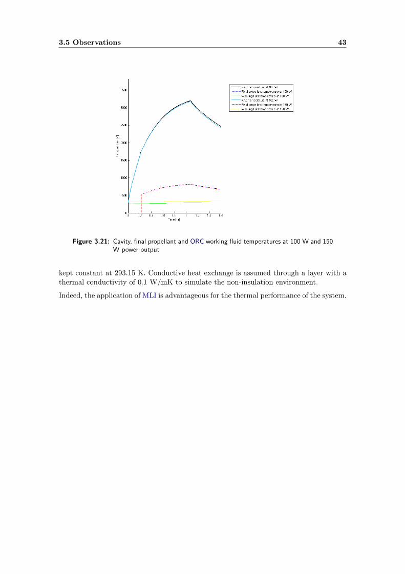
3.5 Observations 43
Figure 3.21: Cavity, final propellant and ORC working fluid temperatures at 100 W and 150W power output
kept constant at 293.15 K. Conductive heat exchange is assumed through a layer with athermal conductivity of 0.1 W/mK to simulate the non-insulation environment.
Indeed, the application of MLI is advantageous for the thermal performance of the system.

44 Design, Analysis and Optimization Tool
Figure 3.22: Final propellant temperatures with different throat radii
3.5.7 Conclusions concerning observations
Concluding from these observations, one can state that an optimal trade-off exists betweenRAC and final propellant temperature. By fine-tuning the variables of specifically Node1 and Node 6 to Node 9 this optimal state can be achieved. Care must also be taken toensure that during the first orbit the RAC and therefore the propellant are heated fastenough. This will result in timely power and thrust generation.In Chapter 5 a number of conceptual designs will be synthesized based on this DAO tool.
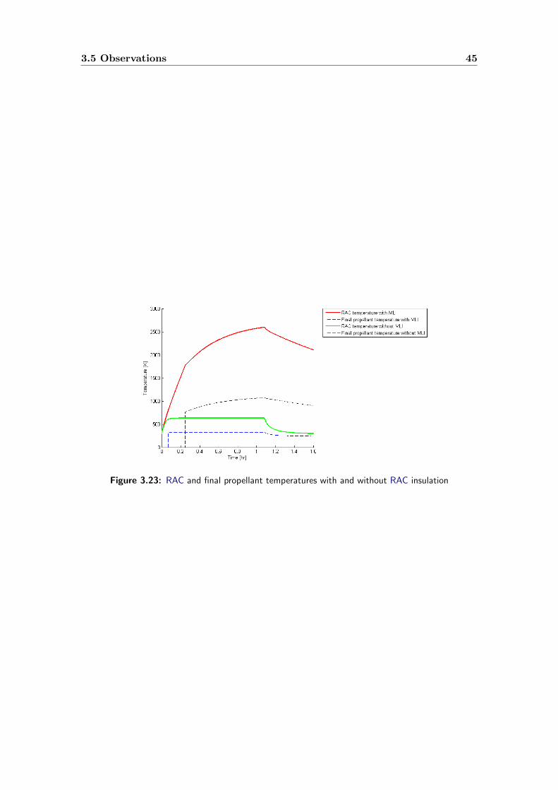
3.5 Observations 45
Figure 3.23: RAC and final propellant temperatures with and without RAC insulation

46 Design, Analysis and Optimization Tool

Chapter 4
Organic Rankine Cycles
An ORC is a means of generating power by the heating of a working fluid and using theresulting increased entropy of the fluid to convert the thermal energy to electrical energy.
Working fluids such as ammonia, hydrocarbons and refrigerants have been applied inthe research of ORC systems (Hung et al. 1997). Saleh et al. (2007) has shown thatthe selection of a working fluid can severely affect the system maximum pressure, fluidmaximum temperature, fluid mass flow and most importantly the thermal efficiency(Mago et al. 2008). Choosing a fluid is therefore critical to the ORC system design.In Angelino & Invernizzi (1993) cyclic methylsiloxanes have been proposed as a propellantsince they have good thermal stability and can operate till a temperature of 400 Celsius.In Rugescu (2012) toluene has been selected as the working fluid because of its goodstability at high temperatures. Furthermore, Rayegan & Tao (2011) has compared a largenumber of candidate working fluids for ORCs and has found that toluene achieves one ofthe highest cycle efficiencies. This fluid is therefore chosen for the upcoming conceptualdesigns.
4.1 Working principles
Each ORC system has the following components. The temperature-entropy plot for atypical simple ORC is given in Figure 4.1. Below each ORC component is matched tothe numbers in the figure.
• Evaporator (2-3) Heat is added to the fluid up to the saturation temperatureafter which it evaporates and the entropy increases at constant temperature; theevaporation takes place at constant pressure
• Turbine (3-4) The working gas expands in the turbine which produces work whichin turn is converted into electrical energy; as a result the entropy increases while thetemperature decreases
• Condenser (4-1) Thermal energy is removed from the working gas at constantpressure until it is once more a fluid in a saturated state
• Pump (1-2) The pump forces the working fluid from the condenser to the evaporatorwhilst increases the pressure of the fluid to evaporator system pressure
47

48 Organic Rankine Cycles
Figure 4.1: Temperature versus entropy plot for simple ORC (Saleh et al. 2007)
If thermal energy storage is required between the thermal energy generator and theevaporator, a thermal exchange cycle can be fitted to the system which releases energyto the evaporator when necessary. In Figure 4.2 one can see a set-up of such a systemwhere a solar collector generates the thermal energy.
Figure 4.2: Schematic for a solar powered ORC system (Wang et al. 2014)
The net power yield of the ORC is the sum of the power output from the turbine and therequired power for the pump. Sign convention dictates that power put into the systemis negative. The power generated by the turbine and the required pump power can becalculated in a simplified way through Equation 4.1 (Kapooria et al. 2008).
P = mwf (hinlet − houtlet) (4.1)
Here, mwf is the working fluid mass flow. The h-terms are the enthalpy of respectivelythe flow in front of the device and the flow behind it.The net power generated by the power subsystem can then be calculated in Equation 4.2(Kapooria et al. 2008). The related system schematic in Figure 4.3 shows the points inthe cycle where the enthalpies are measured.
Pnet = mfluid ((h1 − h2)− (h4 − h3)) (4.2)

4.1 Working principles 49
h = U + pV (4.3)
δh = TδS + V δp (4.4)
In Equation 4.3 one sees that enthalpy itself is the sum of the internal energy (U) andthe achievable work of the fluid. The work is a multiplication of the fluid pressure andvelocity. As such the temperature and pressure of the vaporized working fluid will haveto be traded-off when designing the thermodynamic cycle.
A low inlet pressure at the turbine inlet will mean a high required temperature forthe vapor. A high inlet pressure on the other hand allows the vapor to have a lowertemperature without sacrificing thermal efficiency. A higher inlet pressure requires thickertubing and therefore a larger system mass however.The change in enthalpy in Equation 4.4 is dependent on the temperature, the change inentropy δS and the change in pressure δp. The first term in the equation is the changein internal energy and the second term the change in performed work.
The ORC thermal efficiency ηORC is calculated by taking the total-cycle difference inenthalpy and dividing this by the enthalpy change associated with the input of externalenergy (Equation 4.5). It can also be expressed by the net difference in work dividedby the incoming heat flow (Kapooria et al. 2008). Rayegan & Tao (2011) shows typicalnon-regenerative cycle efficiencies of 12% to 17% at an evaporator temperature of 400 K.Toluene yields an efficiency of 16%. If a higher evaporator temperature is selected, thethermal efficiency will increase.
ηORC =h1 − h2 + h3 − h4
h1 − h4=Wt −Wp
Qin(4.5)
Figure 4.3: Schematic showing measurement points of enthalpy states (Kapooria et al.2008)
Most standard ORC systems operate at relatively low temperatures where the temperaturesof the working fluid reach a maximum of around 250 Celsius depending on the type offluid, as shown by Saleh et al. (2007) and Vaja & Gambarotta (2010). Toffolo et al. (2014)

50 Organic Rankine Cycles
gives a maximum pressure in the turbine ranging from 14 to 67 bar using two differentworking fluids. Mago et al. (2008) and Li et al. (2013) show that the system thermalefficiency increases with increasing turbine inlet pressure. More is elaborated on this inSection 5.2.5.
Another way of increasing the thermal efficiency is the introduction of the process of’regeneration’. It works as follows.The working fluid is still heated up to a gas state in the evaporator. The working gas isforced through the high-pressure turbine stage which lowers the temperature of the gas.At the turbine outlet a small portion of this gas is reintroduced into the evaporator whereit aids the device by pre-heating the relatively colder working fluid. Since not only heat isadded from an external source, the amount of input heat in the evaporator can be reduced.The remainder of the working gas from the turbine outlet is passed to the condenser orto a second low-pressure turbine stage for additional power.At the condenser outlet the gaseous flow will have been converted once more to a saturatedliquid state.As long as the lost work output of the bled working gas does not exceed the decreasein the amount of required external heat in the evaporator, the thermal efficiency will beincreased. Mago et al. (2008) shows this for the working fluids isobutane and R113 whereafter applying regeneration the efficiency is respectively increased from 14% to 15% andfrom 20% to 24%.
Applicable heat exchangers for the evaporator found in literature are a spiral evaporator,a tubular evaporator, a circular nned-tube evaporator, a flat-plate evaporator and aspace-cooled condenser. The evaporators will have to be made of high-conductancematerials and the evaporator chamber itself will have to be highly insulated to preventsevere heat losses. The heat removed at the condenser will have to be fed back into thespacecraft for thermal control purposes or be radiated into space.
While designing the hybrid system, the ORC heat cycle is modelled using an adaptationof the ORCHID-VPE model being developed by the Flight Performance and Propulsiondepartment at DUT’s Faculty of Aerospace Engineering. This model features all thenecessary devices as well as a regenerator. The evaporator and condenser use respectivelya heating and cooling fluid.Geometrical and operational constraints of a small satellite do not allow for a regeneratorand an active-cooling condenser.Therefore the regenerator is deactivated within ORCHID-VPE. Furthermore, the netactive-cooling condenser heat flux is mimicked by a heat flux through a preliminarilydesigned passive space-cooled condenser.
4.2 Condenser performance
In the event that the passive condenser dissipates less heat to space than required theworking fluid temperature in front of the pump will be higher than usual. This case is

4.2 Condenser performance 51
analyzed by comparing two ORC settings at the same turbine inlet pressure and turbineefficiency:
1. The first setting has a turbine inlet temperature and pump inlet temperature ofrespectively 533.15 K and 313.15 K.
2. The second setting on the other hand has a turbine inlet temperature and pumpinlet temperature of respectively 563.15 K and 343.15 K.
Looking at equation 4.2 and 4.4 this means larger enhalpies in front and behind theturbine and pump. The relative difference between the enthalpy at the inlet and outlet ofthe turbine is different for the second setting however since isentropic expansion is takeninto account in the turbine as seen in Equation 4.6.
h2 = h1 − ηturbine(h1 − h2is) (4.6)
Here, ηturbine and h2is are respectively the turbine efficiency and the turbine outletenthalpy under isentropic conditions.Compared to the first setting, a higher temperature produces a larger entropy across theturbine as can be seen in Figure 4.1. As shown earlier a larger entropy generates a largerinternal energy U and therefore a larger h2is for the second setting. This in turn limitsthe decrease of the enthalpy over the turbine in Equation 4.6 and increases h2. Equation4.2 shows that this will decrease the net power.
This is verified since the generated power in the first and second setting is respectively115 W and 105 W.

52 Organic Rankine Cycles

Chapter 5
Conceptual design
In this chapter a number of design concepts with different configurations have beendetailed. Before concepts can be synthesized however an inventory has to be made ofthe system requirements and assumptions.
5.1 Conceptual system requirements and assumptions
5.1.1 Requirements
A total number of six concepts have been designed. All the different RAC configurations,namely conical, cylindrical and spherical, will be featured in these concepts. In addition allthese systems will feature two different propellants, liquid ammonia and liquid hydrogen.
In Section 2.4 the system requirements were put forward. For each concept the propulsionmodule shall deliver at least 1 N in thrust and 100 s in specific impulse. The power budgetshall be a minimum of 100 W. A required ∆V budget of 210 m/s has been previouslystipulated for estimating each concept’s total system mass. Finally, the system shall fitin a 1x1x1m satellite bus.
At this point in the thesis research it is unclear how large the ORC components will be.The power requirement for the ORC’s small turbine are small compared to conventionalturbines which have power outputs in the order of several kW. Therefore a referencemicro-turbine is selected from literature for scaling of the power subsystem.Last, each node must not surpass its maximum operating temperature. In Table 5.1 onecan see the maximum temperatures for the relevant materials. The metals in the tablehave been previously taken into consideration in Section 3.2.2.3 due to their high thermalconductivity and commercial availability.As component temperatures are expected to increase beyond 1400-1500 K, copper isdiscarded as the main constituent material of the concepts. Rather, molybdenum andtungsten are more suitable. In Section 5.2.2 molybdenum and tungsten systems arecompared in terms of their performance.
53

54 Conceptual design
Table 5.1: Maximum operating temperatures for thermal nodes
Material MaximumTemperature [K]
CP-1 and CP-2 Polyimide film (DuPont 2014) 673
Copper (Engineering Toolbox 2000) 1357
Tungsten (Engineering Toolbox 2000) 3673
Molybdenum (Engineering Toolbox 2000) 2893
Sapphire Single-Crystal (Kyocera 2013) 1373
5.1.2 Assumptions
A number of assumptions have been made regarding the preliminary designs as obviouslythe lack of an entire system architecture leads to many unknowns.
5.1.2.1 Mass estimates
The mass estimate for the entire hybrid subsystem is difficult to synthesize due to designunknowns and the lack of reference systems in literature. Therefore an estimate isnecessary. In Table 5.2 the mass budget is given for multiple small satellite missions. Thepropulsion subsystem includes the thruster, feed lines, propellant tank and the propellantitself. The power subsystem includes the electric power system (EPS) and the solar array.
Table 5.2: Reference mass budgets for small satellites
Mass[kg]
Constellation forDisaster Monitoring(Ward et al. 1999)
Proba 3(Bordeet al.2004)
SIMONE(Wellset al.2006)
HummerSat-1 (Zhanget al. 2007)
SMART-1(Raccaet al. 2002)
Power 19.6 21.6 23.3 15.7 96.3
Propulsion 15 13.4 46.2 22.1 111.2
Total 65.5 110.5 120 159.5 366.9
From the table the mean value for a conventional propulsion and the power subsystem isrespectively 21% and 24% of the total spacecraft mass. As stated previously the marginfor the propulsion subsystem takes into account the propellant. Assuming that half thepropulsion subsystem’s wet mass is propellant yields an estimate of 10.5% of the totalspacecraft mass for the dry propulsion subsystem.
The total spacecraft mass is a sum of the 200-kg dry mass and the propellant mass. Thepropellant mass itself has a 20% margin for residual propellant. The tank volume to storethis propellant has a 20% ullage margin of its own.The dry propulsion subsystem mass is a sum of the mass of the system components, theestimated thruster mass and the 10.5% estimate for the dry propulsion subsystem.

5.1 Conceptual system requirements and assumptions 55
A 10% safety margin is added on top of the 10.5% and 24% estimates.
Mpropdry = Mcomponents +Mthruster + 1.1 · 0.105Mtotal (5.1)
Mpower = 1.1 · 0.24Mtotal (5.2)
fsystem =Mpropdry +Mpower
Mtotal(5.3)
The summed up total system mass is divided by the total spacecraft mass which yields asystem mass fraction (Equation 5.3).
5.1.2.2 RAC and interfaces
It is assumed that the central part of the cavity has an interface with the evaporator andthat the entire cavity is insulated with MLI. The insulation has a thickness of 43 mm,a thermal conductivity of 0.1·10−3 W/mK and an effective emittance of 0.002 (Larson &Wertz 2005). The interior of the spacecraft and therefore also the MLI environment isassumed to be at room temperature (293.15 K). Both the radiative and the conductiveheat flux from the RAC through the MLI are taken into account.It is also assumed that there is no radiative heat exchange between a spherical RAC andthe RAC lid and that the conductive heat exchange between this RAC and the lid takesplace at the edge of the lid aperture.
Another assumption is that the conductive interface area between the RAC and thepropellant tubing is a multiplication of the length of the propellant tubing with thetubing-cavity interface width. Although this width was previously established in Section3.4.2, this interface width has been widened to half the propellant tubing radius to takeinto account additional radiative heat transfer as the tubing is relatively small comparedto the adjacent high-temperature RAC.
5.1.2.3 Thermal nodes and tubing conditions
All the nodes are considered isothermal. The temperature profiles for the concepts showthe mean thermal node temperatures; that is, the mean value taken over all the sub-nodetemperatures.
To see the order of magnitude of the thickness of each thermal node, Table 5.5 is provided.Judging from multiple molybdenum tube manufacturers such as Goodfellow (2014) thediameter to minimum wall thickness ratio ranges from 13 to 15. Therefore a ratio of 13will be applied for the cylindrical components such as the pre-cavity chamber and thecavity itself. The propellant tubing gets a smaller factor of 8 (Rembar 2014).The secondary concentrator casing thickness however is defined based on the width of thesecondary concentrator. The cavity lid thickness is one fifth of the cavity radius to ensurethat the MLI which encapsulates the lid can be adequately fastened. The surroundingMLI around the lid has a thickness of 43 mm (Johnson & Fesmire 2011) and a thermalconductivity of 0.1·10−3 W/mK.

56 Conceptual design
For the evaporator and the propellant tubing the minimum thickness is checked whether itcan cope with the internal pressures, using Equation 3.19. The worst-case gas pressure inthe evaporator is assumed to be 10 MPa. For the propellant tubing a maximum pressureis assumed of 20 MPa. Due to the increased tubing temperature the yield strength ofmolybdenum is reduced to around 150 MPa according to test results in Briggs & Campbell(1972). This results in a respective minimum thickness of 0.52 mm and 0.33 mm. This iswell below the actual tube thicknesses (Table 5.5).
Concerning the propellant flow in the tubing adjacent the cavity, turbulent flow as wellas a steady mass flow is assumed. This allows one to use the Sieder-Tate correlation forcalculating the flow’s Nusselt number (Equation 3.40). This number is used to computethe convective heat transfer coefficient between tubing inner wall and the propellant flow.As stated in Chapter 3 the propellant will change phase in the first one-third section ofthe RAC tubing. Therefore in this section latent heat and two-phase flow are taken intoaccount.Furthermore, the initial propellant temperature into the tubing is assumed to be thepropellant storage temperature.The evaporator heating fluid or gas initial temperature is assumed to be 293.15 K beforeconvection.The convection area between RAC and heating gas is assumed to be the area of theheating gas channel which follows the circumference of the RAC; the straight sectionsto and from the ORC evaporator are only for transporting the gas (Figure 5.1). Noradiative heat exchange is assumed between the heating gas channel and the RAC due tothe presence of MLI unless specified otherwise.
Figure 5.1: Schematic of the heating gas channel and RAC interface
5.1.2.4 External fluxes and temperatures
The assumption is made that one starts at the beginning of the daylight part of the orbit.The primary concentrator, secondary concentrator and RAC receive solar radiation, albeit

5.1 Conceptual system requirements and assumptions 57
each at a reduced level due to lens throughput efficiencies. The primary concentrator,secondary concentrator and its casing receive additional Earth albedo and IR radiation.The casing does not receive solar radiation as it is assumed that the primary concentratorcaptures the sunlight before it can hit the casing.
The reference orbit has a 600 km altitude, a 80 degree inclination and a 50 degree initialRAAN (Table 3.1). This produces the time of eclipse at 61.78 minutes from the start ofa new orbit. The eclipse itself lasts almost 32 minutes.Once the eclipse period in the orbit has been reached, no solar flux, Earth albedo andIR radiation will hit the spacecraft for the duration of that period. During this timethe propellant flow is interrupted to curb the decrease of the RAC and propellant tubingtemperatures. This is verified when comparing Figure 5.2 and Figure 5.11. One seesthat the propellant flow does not reach pre-eclipse temperatures and in fact drops intemperature.
Figure 5.2: Thermal node temperatures for Concept 1 with continuous propellant flow afterflow initialisation
The solar flux itself is assumed to be the mean solar flux value over the entire year of1371 W. The on-axis primary concentrator is assumed to be pointed towards the Sunduring the entire daylight-part of the first orbit. Therefore it receives the full flux duringthat time. During the next orbit a different pointing scheme might be used to keep themaximum RAC and propellant temperatures relatively constant to satisfy Requirement 8.After iterating the model the following conditions therefore hold. Note that these valueshave been tailored to the respective conceptual designs.

58 Conceptual design
• For the concepts which use liquid ammonia and have a conical RAC, 68% of theavailable solar flux is required for subsequent orbits.
• For the concepts which use liquid ammonia and have a cylindrical RAC, 79% of theavailable solar flux is required for subsequent orbits.
• For the concept which uses liquid ammonia and has a spherical RAC concepts asolar flux of 96% is required.
• For the concepts which use liquid hydrogen and have a conical RAC, 98% of thesolar flux needs to be received for subsequent orbits.
• For the concepts which use liquid hydrogen and have a cylindrical RAC, 99% of theentire available solar flux is required for subsequent orbits.
• For the remaining spherical concepts which use liquid hydrogen, the full solar fluxis required.
As a consequence of these measures a long-term temperature increase of the RAC andpropellant is prevented.The model also assumes a worst-case scenario where thrust is constantly generated in thedaylight parts of the evaluated period. Therefore, if only a small amount or no thrustis generated during that time, the pointing scheme again must be different compared towhat is described above.
To increase the speed of the simulations some mean temperature values have been calculatedas described below and indicated in Figure 3.8:
• The final propellant temperature upon which the propellant thruster chamber temperatureduring each orbit is based, is equal to the mean propellant temperature during thedaylight part of each orbit.
• The final evaporator heating medium temperature for each orbit is assumed to bethe mean heating medium temperature which is achieved over the entirety of eachorbit. As the mean heating medium temperature changes each orbit, the turbineinlet temperature and power output change each orbit as well. This is taken intoaccount in Section 5.2.5. This means that the system can generate power duringeclipse as long as the heating medium temperature is high enough.
Finally, some assumptions govern the power subsystem in general:
• The mass flow of the ORC’s working fluid is constant.
• A turbine efficiency of 75% is assumed which is in the range as defined in PowerMEMS(2014) and Schubert (2012).
• The pump efficiency is assumed 50% which is in the order of magnitude found inliterature for small pumps such as Kim et al. (2014) and Laser & Santiago (2004).
• A typical pressure loss in the turbine of 2% is assumed.

5.2 General design considerations 59
5.2 General design considerations
In the previous section the requirements and assumptions were put forward. These arefollowed in this section by general design considerations for all the concepts.This includes the definition of the system efficiency, which materials and gases are used,which thruster nozzle shape is adopted and which tubing configuration is selected. Finallysome design parameters for the power subsystem are determined.
5.2.1 System efficiency
The system efficiency of a solar thermal power-propulsion hybrid system defines howefficient the system can convert the inserted solar heat into both power for the otherspacecraft subsystems and thrust for the entire spacecraft. However, no efficiency variablehas so far been defined. In this section an equation will be proposed to define this efficiencyvariable in order to evaluate the efficiency of the different system designs.
First of all the efficiency should include the input solar heat as this is the system’s energysource.Second, the thrust and generated net power should feature in the efficiency equation asthese are the output products of the system.
To convert the thrust to power in Watts, the principle of thrust is summarized.The application of thrust increases the spacecraft’s velocity vector in a certain directionand thereby the kinetic energy of the spacecraft. This in turn alters its orbit, dependingon the direction of the velocity increment. One can therefore use the expression for kineticenergy (Equation 5.4) to derive a power equation as a function of the thrust (Equation5.5).
Ek =1
2mU2 (5.4)
P =1
2T · U (5.5)
Here, Ek is the kinetic energy, m is the mass and U is velocity. The P and T termsindicate the output power and output thrust respectively.All the values except the velocity are straightforward. The velocity-term could concernthe thruster exhaust velocity, the velocity increment ∆V or the orbital velocity.As the orbital velocity is not characteristic for the system but for the spacecraft mission,it is discarded.The thruster exhaust velocity is already used to calculate the thrust as shown in Equation3.92. Therefore, including this velocity would make the influence of the thrust in theefficiency equation far too dominant.Finally, ∆V indicates the amount of total velocity change which can be generated bythe hybrid system. As such it provides a measure of how long thrust can be delivered.When discussing the efficiency of the system, this time-dependency of the thrust cannotbe neglected, as power can be generated constantly.

60 Conceptual design
Concluding, the U in Equation 5.5 becomes ∆V .
Adding the net power to the equation and dividing by the input heat, yields an expressionfor the total system efficiency ηsystem, Equation 5.6.
ηsystem =12T ·∆V + Pnet
S ·Aprimcs(5.6)
Here, T is the thrust in Newtons, ∆V is the velocity increment as defined in Requirement6 and Pnet is the net power generated by the power subsystem. The denominator is thesolar flux hitting the solar concentrator, which may be less than the full solar flux due tothe concentrator pointing direction, multiplied by the cross-sectional area of the primaryconcentrator. One should see Section 5.1.2.4 for how much solar flux hits the primaryconcentrator.
This efficiency value shall be used in this chapter and in Chapter 6 to compare the differentdesigns in terms of energy efficiency.
5.2.2 Materials and constituent fluids and gases
As stated previously molybdenum is a suitable material as it has high thermal conductivityand can cope with high temperatures. The material will therefore feature extensively ineach concept.All the designs have a molybdenum secondary concentrator casing with a white coating.The pre-cavity chamber is also made of molybdenum with a white coating. The molybdenumcavity lid is covered with MLI to limit the temperature of this component and to isolatethe cavity and pre-cavity chamber from each other. The cavity is made of molybdenumwith an interior black paint coating. The propellant tubing is made of molybdenum aswell.
The evaporator heating fluid or gas channel can harbor a fluid or gas. Since phase changesof a heating fluid might induce unpredictable flow behavior, a heating gas is inserted inthe channel. After a short review air is selected as it is cheap and has a relatively largethermal conductivity compared to other gases (Weast 1969).As mentioned in Chapter 4 the ORC’s working fluid will be toluene.To facilitate a large heat flux into the evaporator heating gas, the conduction channelsand heating gas channel are made of molybdenum as well. Although copper provides alarger thermal conductivity, it was found that on most occasions the temperatures of thetwo nodes exceeded copper’s melting point.
In some concepts thermal straps have been implemented so that the temperatures of nodesdo not exceed the maximum operating temperatures during the evaluated time period.One should note that for some concepts the temperature plot for the RAC lid will stillshow an increase during daylight hours and a little decrease in eclipse. This means thatover a long period the maximum operating temperature will be reached. Hence, additionalthermal control measures should be looked at during the detailed design.

5.2 General design considerations 61
Figure 5.3: Thermal node temperatures for Concept 1 with tungsten components
The molybdenum parts can alternatively be replaced with tungsten components.Figure 5.3 and Figure 5.11 show respectively the mean temperatures of the thermal nodesfor a tungsten and a molybdenum design of Concept 1.The performance of the two metals is quite similar except for the higher melting point oftungsten. The figures show virtually no change in the temperature profile. The specificimpulse and thrust remain unchanged when tungsten parts are introduced. The wetsystem mass fraction however increases from 0.61 to 0.69 as molybdenum is a lightermaterial. Therefore molybdenum is preferable; if mass concerns are less importanttungsten can be used as well. In the case of very large primary concentrators andassociated heat fluxes tungsten might be the only option to avoid the melting of components.In the conceptual design phase only molybdenum components will be used as the tungstendesign’s system mass fraction violates Requirement 2.
5.2.3 Nozzle shape
All concepts can have a conical or bell-shaped nozzle. In either case the chamber radiusand pressure are respectively 1 cm and 1 bar. In addition, the throat radius is 1.5 mm. Thenozzle expansion ratio is set at 100. For the conical nozzle the nozzle throat convergenceand the nozzle throat divergence half angle are respectively 25 degrees and 17 degrees.For the bell-shaped nozzle, the nozzle throat convergence half angle is also 25 degrees.The nozzle throat divergence half angle is increased to 35 degrees. The exhaust divergenceangle becomes 11 degrees.The two designs are shown in Figure 5.4 and Figure 5.5. Both nozzles have a length of6.3 cm.

62 Conceptual design
The conditions in the nozzles are such that the Mach number in the throat is 1 and thattherefore the flow velocity also increases in the divergent section.
Figure 5.4: Conical nozzle design Figure 5.5: Bell-shaped nozzle design
In Table 5.3 the nozzle shapes are compared in terms of the maximum values of the specificimpulse, total impulse, thrust and system efficiency. Both nozzles have been applied toConcept 1.
Table 5.3: Performance comparison between a conical and bell-shape nozzle for the samehybrid system
Nozzle Specificimpulse[s]
Totalimpulse[kNs]
Thrust[N]
Systemefficiency[-]
Conical 162 53 1.267 0.42
Bell-shape 169 51 1.273 0.42
One sees that the bell-shape nozzle generates more specific impulse and slightly less totalimpulse. The thrust is larger than the thrust of the conical nozzle and it has the sameefficiency. Sutton & Biblarz (2001) also considers bell-shaped nozzles preferable aboveconical nozzles. The main downside of these nozzles however is that they are more difficultto manufacture.
In Figure 5.6 and Figure 5.7 the propellant flow velocity is shown at the end of the secondorbit for respectively the conical and bell-shaped nozzle.

5.2 General design considerations 63
Figure 5.6: Propellant flow velocityin the conical nozzle forConcept 1
Figure 5.7: Propellant flow velocity inthe bell-shaped nozzle forConcept 1
Although the bell-shaped nozzle achieves a better performance, a conical shape is chosenfor the conceptual designs to keep the number of concepts limited, as there are a lot ofdifferent bell shapes possible. The bell-shaped nozzle will however be considered againwhen discussing the detailed design as it is more advantageous. For comparative purposeshowever the type of nozzle is less significant.
5.2.4 Tubing configuration
All concepts feature a spiral tubing configuration with 20 turns. Note that the statednumber of turns does not take into account the assumed 8% losses in tubing length dueto geometrical constraints (Section 3.2.3.1). The spiral set-up allows for a higher orequivalent propellant temperature compared to the linear tubing, since the spiral patternproduces a relatively large tubing length and conductive area with the cavity. The use ofthis configuration has also been recommended by Leenders & Zandbergen (2008).
One can compare the performance of the same concept with different tubing configurationsto show this.Concept 1 is fed with ammonia propellant and the tubing configuration is changed fromrespectively ’spiral’ to ’linear’ and the number of feed lines is set at 10. This results in aslight decrease of the final propellant temperature at the end of the daylight part of thethird orbit from 734 to 680 K and a small decrease of the specific impulse from 162 to156 s.
For hydrogen concepts the same holds. A comparison of Figure 5.28 and Figure 5.8 showsthe changed temperature profile for Concept 3. When linear tubing with 20 feed lines isapplied the final RAC temperature before eclipse is higher and the temperature increasesevery orbit. This indicates that there is less heat being transferred to the propellanttubing than when spiral tubing is used.Indeed when the design switches to a linear tubing configuration the propellant temperaturedecreases from 908 K to 856 K with a specific impulse decrease from 181 to 175 s at the

64 Conceptual design
Figure 5.8: Temperature of thermal nodes for Concept 3 with a linear configuration with 20propellant tubes
start of eclipse in the third orbit.Only by setting the number of linear tubes to 30 and hence increasing the mass of thetubing can the same propellant temperature and specific impulse be achieved as with thespiral tubing.
Finally, a linear tubing configuration requires an additional flow divider which feeds theinitial propellant flow from the propellant tank to the different tubes alongside the cavity.This increases the complexity of the system and increases the chance of flow disturbanceswhich are both undesirable.Therefore, one can conclude that overall a spiral tubing configuration is more advantageous.
5.2.5 Power subsystem
In the power subsystem a number of design parameters stay constant throughout theconceptual design phase.First of all, the evaporating pressure of the ORC is set at 13.67 bar. In addition, theheating gas flow enters the evaporator at a pressure of 1 bar. This yields a thermalefficiency of 16.8% which falls in the range defined in Chapter 4. Beyond this pressurethe thermal efficiency no longer increases substantially as can be seen in Figure 5.9.Second, the initial turbine inlet temperature is set at 533.15 K for the first orbit. Theturbine inlet temperature will be increased with a scaled term based on the difference inmean heating gas temperature between the first and current orbit, as shown in Equation5.7. The maximum increase in temperature of 90 K has been taken as the turbine inlet

5.2 General design considerations 65
Figure 5.9: ORC thermal efficiency versus evaporating pressure for Concept 1
temperature in ORCs for toluene has an operating maximum of 350 Celsius (Lai et al.2011).
Tturbine−inlet = 533.15 + 90 ·|Theating−gas(norbit)− Theating−gas(1)|
Theating−gas(1)(5.7)
The equation gives an indication of the increased turbine power output when the heatinggas temperature is increased in the system. As the detailed design of and heat exchangeprocess within the evaporator is unknown, the exact increased power output cannot becalculated at this point.
The ORCHID-VPE model assumes active fluid cooling in the condenser. Passive condensercooling is however more advantageous in this hybrid system as has already been indicatedin Chapter 4.Passive condenser convection processes are used to transfer heat from the hot workingfluid to the cooler working fluid tubing inner wall. Through conduction this heat istransferred to the tubing outer wall. Afterwards a conducting or radiating channel willconduct or radiate the heat away. The heat will be dissipated into space via some sort ofradiator on the spacecraft’s exterior. Alternatively, the heat is fed back into the spacecraftfor thermal control. One assumes that the heat between the condenser and radiator isexchanged in the in-plane direction. This must result in a temperature of around 313 Kfor the working fluid behind the condenser.To achieve a power output of at least 100 W a working fluid mass flow of 59 mL/min isnecessary. This value stays constant throughout the evaluated time period.For the conceptual design, only the required dissipated heat flux will be taken into account.

66 Conceptual design
The detailed design of the condenser will be detailed in Chapter 6.
5.3 Concepts
This section will detail the different concepts. The design parameters can be found inAppendix B.The thermal nodes and the concepts are first summarized, followed by the detailing ofthe concepts themselves.
5.3.1 Thermal nodes and summary of the concepts
Figure 5.10 illustrates the overall concept. One can distinguish the primary concentrator,secondary concentrator, RAC, propellant tank and tubing, the thruster and the ORCpower subsystem components. Note that the concepts include a conductive interfacebetween the RAC and evaporator heating gas channel; in the detailed design this interfacemight be replaced by a radiative interface.
The identifiers represent the following components or phenomena:
1: Primary concentrator2: Secondary concentrator3: Secondary concentrator casing4: Pre-cavity chamber5: Cavity lid6: RAC7: Propellant tubing8: Evaporator heat conducting channel9: Evaporator (heating gas channel)10: Condenser (working fluid channel)11: Condenser heat conducting/radiatingchannel12: Turbine13: Pump14: Propellant tank15: Propellant feed lines16: Thruster chamber17: Thruster nozzleP: Power [W]S: Solar flux [W]T: Thrust [N]Q: Heat flux [W]
A summary of the conceptual designs is given in Table 5.4.In Section 5.3.2 to Section 5.3.7 these designs will be elaborated upon, including theirperformance.
Note that the power generation and dissipated heat from the ORC have been displayedbased on their mean value over an entire orbit to limit the model’s computational time.

5.3 Concepts 67
Figure 5.10: Concept schematic with conical RAC configuration
Table 5.4: Summary of the conceptual designs
Concept RAC shape Tubing configuration Propellant
1 Conical Spiral Liquid ammonia
2 Conical Spiral Liquid hydrogen
3 Cylindrical Spiral Liquid ammonia
4 Cylindrical Spiral Liquid hydrogen
5 Spherical Spiral Liquid ammonia
6 Spherical Spiral Liquid hydrogen
5.3.2 Concept 1
The first concept utilizes a conical RAC. The propellant liquid ammonia is cryogenicallystored at 243 K. The thickness of some nodes are given in Table 5.5 to give one a senseof the order of magnitude of the dimensions involved.
In Figure 5.11 the temperature profile is shown for all the thermal nodes in the propulsionsubsystem. Figure 5.12 and 5.13 show a geometrical mesh of the front and rear of thesubsystem excluding the primary concentrator and the thruster. The temperatures ofthe thermal nodes after one hour of flight time are incorporated. The coordinates in thefigure are with respect to the center of the outer extremity of the primary concentrator.The black components represent the other side of the system whose temperatures exceedthe temperature scale.

68 Conceptual design
Table 5.5: Component thickness
Component Thickness [mm]
Secondary concentrator casing 4.3
Pre-cavity chamber 10.8
RAC lid 14.0
RAC 10.8
Propellant tubing 0.625
Heating gas channel 1.2
Figure 5.11: Temperature of thermal nodes for Concept 1
Figure 5.12: Thermal mesh rear viewat 60 minutes after modelinitialisation for Concept 1
Figure 5.13: Thermal mesh front viewat 60 minutes after modelinitialisation for Concept 1

5.3 Concepts 69
The figures below represent the thrust, power, specific impulse for the concept. Thetotal impulse is 53 kNs evaluated over the period required to propel all the propellant.The thrust plot shows constant values since the final propellant temperature stays fairlyconstant throughout each orbit, meaning that the chamber temperature stays fairlyconstant as well. The mass flow in the nozzle is 820 mg/s.
Figure 5.14: Thrust and powergeneration for Concept 1
Figure 5.15: Specific impulse forConcept 1
One can see in Figure 5.14 that after the first orbit, where the system has to adjust tothe increased temperatures, a more or less constant mean power generation of 115 Wis achieved. The thrust stays constant at 1.267 N. In Figure 5.15 the initial maximumspecific impulse of 160 s increases to 162 s in the third orbit.The system efficiency is given in Figure 5.16. The maximum efficiency varies between0.19 in eclipse to 0.42 in daylight.
Figure 5.16: System efficiency for Concept 1
The mean dissipated heat out of the ORC condenser is plotted in Figure 5.17. Thedissipated heat flux moves to a stable value of 566 W.
Finally, the required propellant storage volume, the dry system mass and the wet systemmass fraction are respectively 0.06 m3, 109 kg and 0.61.

70 Conceptual design
Figure 5.17: Mean dissipated heat out of ORC condenser for Concept 1
In the conceptual designs hydrogen and ammonia are used as propellants for their advantageousperformance. Both propellants have to be cryogenically stored which puts more structuralrequirements on the spacecraft. Therefore, for a complete analysis water and hydrogenare applied to Concept 1 to see which system requirements can still be met with thesenon-cryogenic propellants.
5.3.2.1 Performance with water as non-cryogenic propellant
Water has a latent heat of vaporization of 2257 kJ/kg. Therefore the tubing convectionarea has to increase substantially for Concept 1 in order to overcome the vaporizationof the liquid water and increase the temperature of the resulting water vapor to achievesufficient thrust.Water in a liquid state has a high thermal conductivity. As the temperature differencebetween the propellant and the propellant tubing will be in the order of several hundredsof Kelvin, a large heat flux between the tubing and water is expected. The propellantwill therefore evaporate quickly in the spiral tubing. The assumption is therefore madethat within the RAC-adjacent tubing water is in a gaseous state and that therefore thegaseous properties are used outside of the propellant tank.
First, the radius of the evaporator heating gas channel and its conducting channels areset at respectively 7.8 mm and 7.0 mm. The solar flux from the second orbit onwards is58% of the full amount.In Figure 5.18 the temperature profile is shown for the Concept 1 thermal nodes whenwater is selected as propellant. Note that the applicable water vapor properties apply fora vapor temperature of around 1000 K.
The power and thrust generated in the third orbit are respectively 114 W and 1.272 N.The specific impulse settles to a value of 148 s. As expected the specific impulse is lowerthan for ammonia. The system-specific impulse is 64 s which is slightly lower than forthe original Concept 1.The system efficiencies are higher than the efficiencies of the original Concept 1. In

5.3 Concepts 71
Figure 5.18: Thermal node temperatures for Concept 1 with water as propellant
daylight and eclipse they are respectively 0.49 and 0.23. The propellant tank volume issmaller than for ammonia at 0.045 m3.The wet system mass is 62% of the total mass, satisfying Requirement 2.
Unfortunately this performance has been achieved with a spiral tubing configuration with80 turns which is very difficult to accurately manufacture. The large number of turns iscaused by the fact that the system must overcome water’s high latent heat and musttherefore insert more heat into the propellant. A larger heat input requires a largerconvective area and hence longer tubing. One should also note that water will freezeto a solid state below 273.15 K. If this were to occur propellant flow would be severelyimpeded, compromising thrust ability.Therefore, there will have to be sufficient insulation and heating devices applied to thepropellant tank to keep the water in the appropriate temperature range. The initialadvantage of not having to apply cryogenic storage solutions is therefore replaced byother thermal control difficulties.Water is therefore not an ideal propellant for this system.
5.3.2.2 Performance with nitrogen as non-cryogenic propellant
In this iteration nitrogen is uses as propellant. As a consequence the radius of theevaporator heating gas channel and its conducting conduits are set at respectively 11.7mm and 5.8 mm. In the second and third orbit only 71% of the total solar flux is used.The power and thrust in the third orbit are 116 W and 1.213 N. The concept’s maximumspecific impulse settles to a value of 160 s. The system-specific impulse is 65 s which is

72 Conceptual design
smaller than for water.The efficiency in daylight and eclipse are respectively 0.39 and 0.19. The wet system massfraction is 0.62. Figure 5.19 gives the associated temperature plots.
Figure 5.19: Thermal node temperatures for Concept 1 with nitrogen as propellant
Unfortunately nitrogen has a very low density. Therefore the required propellant storagevolume is 35 m3 at 1-bar storage pressure which is off-course too large for the spacecraftbus and violates Requirement 1. Using the ideal gas law yields a pressure of 35 MPa foran acceptable storage volume of 0.10 m3. This pressure will increase the propellant tankthickness substantially and as a consequence increase the mass of the system. This makesthis propellant option undesirable, even though it satisfies the other system requirements.
The next section continues the performance evaluation of the conceptual designs.
5.3.3 Concept 2
Just as Concept 1, Concept 2 utilizes a conical RAC. The propellant here is liquidhydrogen and it is cryogenically stored at 17 K. In Figure 5.21 the temperature profilefor all the thermal nodes in the propulsion subsystem have been given.Figure 5.22 and Figure 5.23 show again a geometrical mesh of the front and rear of thesubsystem including temperatures. To limit the increase of the secondary concentratortemperature ten thermal straps have been attached to the concentrator circumference.The length of the thermal straps is 13 cm, their cross-section is 3.6x5 mm and their thermalconductivity is 400 W/mK as a copper-like material is assumed. Its sink temperature is

5.3 Concepts 73
set at 293.15 K, the assumed local temperature within the spacecraft.
Figure 5.20: Illustration of thermal straps interfaced with the secondary concentrator
Figure 5.22: Thermal mesh rear viewat 60 minutes after modelinitialisation for Concept 2
Figure 5.23: Thermal mesh front viewat 60 minutes after modelinitialisation for Concept 2
Below the thrust, power and specific impulse performance for the concept have beenshown. The total impulse becomes 50 kNs. The nozzle mass flow is substantially lowerat 190 mg/s compared to the 820 mg/s for Concept 1.

74 Conceptual design
Figure 5.21: Temperature of thermal nodes for Concept 2
Figure 5.24: Thrust and powergeneration for Concept 2
Figure 5.25: Specific impulse forConcept 2
One can see in Figure 5.24 that after the first orbit, in which the system has to adjust tothe increased temperatures, a more or less constant mean power generation of 108 W isachieved. The thrust stays constant at 1.209 N. The specific impulse is shown in Figure5.25. The initial maximum specific impulse of 657 s stays constant over the evaluatedperiod.
The system efficiency is given in Figure 5.26. The efficiency varies between 0.04 in eclipseto 0.09 in daylight which is substantially lower than for Concept 1.

5.3 Concepts 75
Figure 5.26: System efficiency for Concept 2
The mean dissipated heat out of the ORC condenser is plotted in Figure 5.27. Thedissipated heat flux starts at 507 W and increases to a value of 531 W in the third orbit.
Figure 5.27: Mean dissipated heat out of ORC condenser for Concept 2
Concluding this concept, the required propellant storage volume, the system mass andthe system mass fraction are respectively 0.13 m3, 101 kg and 0.53.
5.3.4 Concept 3
Concept 3 has a cylindrical RAC. The used propellant is liquid ammonia. In Figure 5.28the temperature profile for all the thermal nodes in the propulsion subsystem have beengiven. The first orbit has a maximum RAC temperature of 1365 K which stays relativelyconstant over the subsequent orbits.Figure 5.29 and 5.30 show the geometrical mesh of the subsystem excluding the primaryconcentrator and the thruster and with the thermal node temperatures incorporated.

76 Conceptual design
Figure 5.28: Temperature of thermal nodes for Concept 3
Figure 5.29: Thermal mesh rear viewat 60 minutes after modelinitialisation for Concept 3
Figure 5.30: Thermal mesh front viewat 60 minutes after modelinitialisation for Concept 3
The figures below show the performance for this design. Calculations yield a maximumtotal impulse of 52 kNs. The propellant mass flow is calculated to be 730 mg/s.
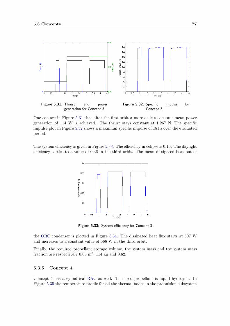
5.3 Concepts 77
Figure 5.31: Thrust and powergeneration for Concept 3
Figure 5.32: Specific impulse forConcept 3
One can see in Figure 5.31 that after the first orbit a more or less constant mean powergeneration of 114 W is achieved. The thrust stays constant at 1.267 N. The specificimpulse plot in Figure 5.32 shows a maximum specific impulse of 181 s over the evaluatedperiod.
The system efficiency is given in Figure 5.33. The efficiency in eclipse is 0.16. The daylightefficiency settles to a value of 0.36 in the third orbit. The mean dissipated heat out of
Figure 5.33: System efficiency for Concept 3
the ORC condenser is plotted in Figure 5.34. The dissipated heat flux starts at 507 Wand increases to a constant value of 566 W in the third orbit.
Finally, the required propellant storage volume, the system mass and the system massfraction are respectively 0.05 m3, 114 kg and 0.62.
5.3.5 Concept 4
Concept 4 has a cylindrical RAC as well. The used propellant is liquid hydrogen. InFigure 5.35 the temperature profile for all the thermal nodes in the propulsion subsystem

78 Conceptual design
Figure 5.34: Mean dissipated heat out of ORC condenser for Concept 3
has been shown.Figure 5.36 and 5.37 show the geometrical mesh of the subsystem, excluding the primaryconcentrator and the thruster and including thermal node temperatures.As in Concept 2 ten thermal straps have been added to decrease the secondary concentratortemperature so that it does not violate its maximum temperature.
Figure 5.35: Temperature of thermal nodes for Concept 4
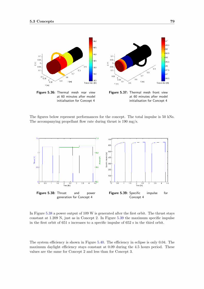
5.3 Concepts 79
Figure 5.36: Thermal mesh rear viewat 60 minutes after modelinitialisation for Concept 4
Figure 5.37: Thermal mesh front viewat 60 minutes after modelinitialisation for Concept 4
The figures below represent performances for the concept. The total impulse is 50 kNs.The accompanying propellant flow rate during thrust is 190 mg/s.
Figure 5.38: Thrust and powergeneration for Concept 4
Figure 5.39: Specific impulse forConcept 4
In Figure 5.38 a power output of 109 W is generated after the first orbit. The thrust staysconstant at 1.209 N, just as in Concept 2. In Figure 5.39 the maximum specific impulsein the first orbit of 651 s increases to a specific impulse of 652 s in the third orbit.
The system efficiency is shown in Figure 5.40. The efficiency in eclipse is only 0.04. Themaximum daylight efficiency stays constant at 0.09 during the 4.5 hours period. Thesevalues are the same for Concept 2 and less than for Concept 3.

80 Conceptual design
Figure 5.40: System efficiency and effective exhaust velocity for Concept 4
The mean dissipated heat out of the ORC condenser is plotted in Figure 5.41. Thedissipated heat flux increases from 507 W to a constant 535 W.
Figure 5.41: Mean dissipated heat out of ORC condenser for Concept 4
Concluding, the required propellant storage volume, the system mass and the systemmass fraction are respectively 0.14 m3, 106 kg and 0.55.
5.3.6 Concept 5
Concept 5 has a spherical RAC. The propellant is liquid ammonia. In Figure 5.42 thetemperature profile for all the thermal nodes is given.Figure 5.43 and 5.44 show the geometrical mesh for Concept 5, including thermal nodetemperatures.

5.3 Concepts 81
Figure 5.42: Temperature of thermal nodes for Concept 5
Figure 5.43: Thermal mesh rear viewat 60 minutes after modelinitialisation for Concept 5
Figure 5.44: Thermal mesh front viewat 60 minutes after modelinitialisation for Concept 5
The figures below represent performances for the concept. Calculations yield a totalimpulse of 52 kNs. Here, the propellant mass flow decreases even further to 630 mg/scompared with 820 mg/s for Concept 1.

82 Conceptual design
Figure 5.45: Thrust and powergeneration for Concept 5
Figure 5.46: Specific impulse forConcept 5
A power output of 104 W is generated in the first orbit. In the orbits thereafter the turbinegenerates around 110 W. As expected, the thrust stays constant at 1.267 N. The specificimpulse plot shows a constant maximum specific impulse of 208 s just before every eclipse.
The system efficiency is given in Figure 5.47. The efficiency in eclipse is only 0.13. Themaximum daylight efficiency stays constant after each orbit at 0.29.
Figure 5.47: System efficiency for Concept 5
The mean dissipated heat out of the ORC condenser is plotted in Figure 5.48. Thedissipated heat flux increases from 507 W in the first orbit to 541 W in the third orbitrespectively.
Finally, the required propellant storage volume, the system mass and the system massfraction are respectively 0.05 m3, 99 kg and 0.55.

5.3 Concepts 83
Figure 5.48: Mean dissipated heat out of ORC condenser for Concept 5
5.3.7 Concept 6
Concept 6 also has a spherical RAC. The propellant is liquid hydrogen. In Figure 5.49the temperature profile is given for all the thermal nodes in the propulsion subsystem. Amaximum propellant temperature of 1661 K is achieved.Figure 5.50 and 5.51 show the geometrical mesh of the subsystem, including thermal nodetemperatures.As in the other hydrogen concepts ten thermal straps have been added to decrease thesecondary concentrator temperature. Since this has limited effect, more thermal strapswill have to be added in the detailed design if this concept is selected.
Figure 5.49: Temperature of thermal nodes for Concept 6

84 Conceptual design
Figure 5.50: Thermal mesh rear viewat 60 minutes after modelinitialisation for Concept 6
Figure 5.51: Thermal mesh front viewat 60 minutes after modelinitialisation for Concept 6
The figures below represent performances for the concept. The total impulse for thisconcept is 50 kNs. During thrust the propellant mass flow in the nozzle is 190 mg/s.
Figure 5.52: Thrust and powergeneration for Concept 6
Figure 5.53: Specific impulse forConcept 6
In Figure 5.52 a power output of 107 W is generated after the 4.5-hour period. Thethrust stays constant during this time at 1.209 N as one has seen with the other hydrogenconcepts. The specific impulse plot in Figure 5.53 shows a stable maximum specificimpulse of 660 s before eclipse.
The system efficiency is given in Figure 5.54. The eclipse efficiency is 0.04 and the daylightefficiency is 0.09 which is the same as for Concept 2 and Concept 4.
The mean dissipated heat out of the ORC condenser is plotted in Figure 5.55. Thedissipated heat flux starts at 507 W. It then increases to 522 W in the third orbit.
Finally, the required propellant storage volume, the system mass and the system massfraction are respectively 0.13 m3, 94 kg and 0.49.

5.4 Mass and size comparison of concepts 85
Figure 5.54: System efficiency for Concept 6
Figure 5.55: Mean dissipated heat out of ORC condenser for Concept 6
5.4 Mass and size comparison of concepts
Although the mass and size between the concepts vary relatively little, the two propertiesneed to be taken into account at this phase in the design process. First the mass will bediscussed; afterwards a section will detail the size of each concept.
5.4.1 Mass of the concepts
The mass of the concepts is currently evaluated based on three indicators:
1. Total mass The total mass of the spacecraft, including propellant
2. Wet system mass The mass of the hybrid propulsion and power system, includingpropellant
3. Wet system mass fraction Mass fraction of the hybrid propulsion and power system,including the propellant, with respect to the total spacecraft mass

86 Conceptual design
Table 5.6 details the different mass indicators for each concept.All concepts satisfy Requirement 2. Given that the current mass estimates are mostlyderived from the propellant mass, the concepts with liquid hydrogen propellant arepreferable in terms of absolute mass over the concepts with liquid ammonia. The liquidammonia concepts also have a higher wet mass fraction.In terms of absolute total mass Concept 2, 4 and Concept 6 are the lightest. The lightestwet system mass is achieved with Concept 5 and Concept 6. The smallest mass fractionsare achieved with Concept 2 and Concept 6.
Table 5.6: Mass comparison of the concepts
Concept TotalMass [kg]
Propellantmass [kg]
Drysystemmass [kg]
Wet systemmassfraction[-]
1 234 34 109 0.61
2 208 8 101 0.53
3 230 30 114 0.62
4 208 8 106 0.55
5 226 26 99 0.55
6 208 8 94 0.49
5.4.2 Size of the concepts
First, size can be evaluated by determining the footprint of the system in the spacecraft.The footprint is defined as the top-view area of an imaginary box around the systembeyond which the system does not interfere with other spacecraft subsystems. Figure5.56 illustrates this.
Figure 5.56: Illustration of the system’s footprint
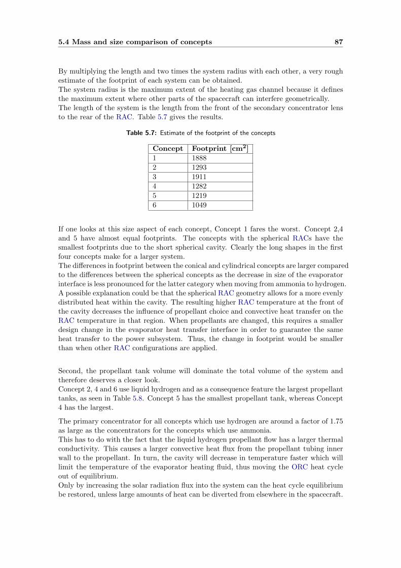
5.4 Mass and size comparison of concepts 87
By multiplying the length and two times the system radius with each other, a very roughestimate of the footprint of each system can be obtained.The system radius is the maximum extent of the heating gas channel because it definesthe maximum extent where other parts of the spacecraft can interfere geometrically.The length of the system is the length from the front of the secondary concentrator lensto the rear of the RAC. Table 5.7 gives the results.
Table 5.7: Estimate of the footprint of the concepts
Concept Footprint [cm2]
1 1888
2 1293
3 1911
4 1282
5 1219
6 1049
If one looks at this size aspect of each concept, Concept 1 fares the worst. Concept 2,4and 5 have almost equal footprints. The concepts with the spherical RACs have thesmallest footprints due to the short spherical cavity. Clearly the long shapes in the firstfour concepts make for a larger system.The differences in footprint between the conical and cylindrical concepts are larger comparedto the differences between the spherical concepts as the decrease in size of the evaporatorinterface is less pronounced for the latter category when moving from ammonia to hydrogen.A possible explanation could be that the spherical RAC geometry allows for a more evenlydistributed heat within the cavity. The resulting higher RAC temperature at the front ofthe cavity decreases the influence of propellant choice and convective heat transfer on theRAC temperature in that region. When propellants are changed, this requires a smallerdesign change in the evaporator heat transfer interface in order to guarantee the sameheat transfer to the power subsystem. Thus, the change in footprint would be smallerthan when other RAC configurations are applied.
Second, the propellant tank volume will dominate the total volume of the system andtherefore deserves a closer look.Concept 2, 4 and 6 use liquid hydrogen and as a consequence feature the largest propellanttanks, as seen in Table 5.8. Concept 5 has the smallest propellant tank, whereas Concept4 has the largest.
The primary concentrator for all concepts which use hydrogen are around a factor of 1.75as large as the concentrators for the concepts which use ammonia.This has to do with the fact that the liquid hydrogen propellant flow has a larger thermalconductivity. This causes a larger convective heat flux from the propellant tubing innerwall to the propellant. In turn, the cavity will decrease in temperature faster which willlimit the temperature of the evaporator heating fluid, thus moving the ORC heat cycleout of equilibrium.Only by increasing the solar radiation flux into the system can the heat cycle equilibriumbe restored, unless large amounts of heat can be diverted from elsewhere in the spacecraft.

88 Conceptual design
Table 5.8: Size comparison of the concepts
# Systemlength inX [cm]
Width inY or Z[cm]
Primaryconcentratordiameter [m]
Diameterof turbine[mm]
Propellanttank volume[m3]
1 45.91 20.56 0.90 19 0.06
2 46.19 14.00 1.57 19 0.13
3 45.51 21.00 0.90 19 0.05
4 45.79 14.00 1.57 19 0.14
5 32.51 18.75 0.90 19 0.05
6 32.79 16.00 1.57 19 0.13
5.5 Performance comparison of concepts
Not only the mass and size of the system are important. One also needs to look at whetherthe concepts exceed Requirement 3 to 6 and to what degree they exceed them. This willalso give an idea about scalability of each design.In Table 5.9 the performance of each concept in terms of the three parameters is stated.The condenser dissipated flux in Watts has been included as has been the daylight systemefficiency.The system-specific impulse is shown in Table 5.10.
Table 5.9: Performance comparison of the concepts
# Thrust[N]
Specificimpulse [s]
Power[W]
Condenser dissipatedflux [W]
Efficiency[%]
1 1.267 162 115 566 42
2 1.209 657 108 531 9
3 1.267 181 114 566 36
4 1.209 652 109 535 9
5 1.267 208 110 541 29
6 1.209 660 107 522 9
As can be seen in the table all concepts satisfy Requirement 3 to 5. Concept 5 and 6 havethe highest specific impulse in their respective class of concepts with the same propellant.The mean power output after three orbits is slightly higher for the ammonia concepts.The liquid hydrogen concepts generate more specific impulse and slightly less thrust. Thisis as expected as hydrogen has a higher specific heats ratio and thermal conductivity thanammonia.The system efficiency is the highest for Concept 1 and decreases for the other ammoniaconcepts. The efficiencies for all the hydrogen concepts are the lowest at 9%. One cantherefore conclude that the hydrogen concepts convert the inserted solar energy the leastefficiently to power and thrust.
In Table 5.10 the total impulse and system-specific impulse are given for each conceptto compare the concepts from a system-perspective. The total impulse also takes into

5.6 Scalability 89
account the total thrust time. One sees that the hydrogen concepts generate a smallertotal impulse but produce a larger system-specific impulse. This means that these conceptsgenerate more impulse per kg of propulsion subsystem. A larger value is thereforeadvantageous for the total mass budget of the spacecraft. Concept 6 in this regardproduces the largest system-specific impulse.
Table 5.10: System-specific impulse and related variables for the concepts
# Wet propulsionsystem mass [kg]
Total impulse[kN·s]
System-specificimpulse [s]
1 81 53 66
2 54 50 94
3 83 52 65
4 59 50 87
5 66 52 80
6 47 50 108
In terms of the recovery of cavity and propellant temperatures after eclipse all conceptshave been tailored to a fast temperature recovery with close-to-equal maximum propellanttemperatures just before each orbit’s eclipse.The concepts with thermal straps limit the increase of the secondary concentrator andpre-cavity chamber somewhat. Concepts without thermal control devices see an increaseof these components over time. As Concept 5 and Concept 6 have no heat transferbetween the lid and the RAC, the lid’s temperature stays constant. In the other conceptsthe cavity lid increases almost linearly over time. Further thermal control must hence beexercised in the detailed design.
Not only thermal control of the propulsion subsystem must be performed. Thermalcontrol of other parts of the spacecraft is also necessary. Batteries for example onlywork in temperatures from about -5 to +15 degrees Celsius. Thermal control of othersubsystems can include diverting the dissipated heat from the passive condenser in thepower subsystem to other regions of the spacecraft interior. Looking at Table 5.9, Concept1 and Concept 3 can dissipate the most heat in this regard.
5.6 Scalability
This section deals with the scalability of the system. Since power, thrust and specificimpulse are the KPPs in terms of system performance, scalability will be discussed interms of these parameters.Concept 1 will be used as a reference to scale the system. The focus in each subsectionis solely on whether the increase of the specific performance parameter is feasible; otherperformance parameters or component constraints have not been looked into.Table 5.11 and 5.12 give a summary of the results, excluding in terms of the specificimpulse.

90 Conceptual design
5.6.1 Power
First, the required power output of the turbine will be increased from 100 W to 200W. Second, it will be further increased from 200 W to 400 W to see whether a scalingrelationship exists.When the power is increased to 200 W, the primary concentrator diameter needs toincrease from 0.9 m to 1.0 m. The cavity radius stays constant at 7 cm. The heating gaschannel radius increases from 7.8 mm to 14 mm. The evaporator conducting channels’radius is increased from 7 mm to 11.7 mm.The power subsystem’s working fluid mass flow needs to increase from 59 mL/min to 118mL/min. The turbine diameter increases from 19 mm to 27 mm. The dissipated powerincreases from 566 W to 1083 W.
Second, the power is increased further to 400 W. The cavity radius stays constant at 7cm. The primary concentrator diameter increases from 1.0 m to 1.1 m. The evaporatorheating gas channel’s radius is increased from 14 mm to 23.3 mm and the evaporatorconducting channels’ radius is increased from 11.7 mm to 14.0 mm.The micro-turbine diameter becomes 38 mm. This is twice the diameter for a poweroutput 1/4 the current one. Furthermore the working fluid mass flow increases further to236 mL/min. Calculations yield a required dissipated heat flux out of the working fluidof 2104 W.
The 1083 W and 2104 W are very large fluxes for a radiator mounted to a 1x1x1 m bus tocope with. Therefore, radiator fins or deployable radiators will be necessary to dissipatethe heat. This will add to the satellite mass. Thus, scalability is limited for a smallsatellite beyond power levels of around 100 W.
Increasing the primary concentrator diameter, increasing the size of the evaporator conductingchannel and enlarging the condenser allows theoretically for an even larger power output.One should however note that a larger system will decrease the available spacecraft volumefor instruments and increase the complexity of deploying a larger primary concentrator.Furthermore, the external radiators will increase in number and/or size.
Table 5.11: Scalability results in terms of power
Power[W]
Dissipationheat flux[W]
Primaryconcentratordiameter [m]
Turbinediameter[mm]
Working fluidmass flow[mL/min]
100 566 0.9 19 59
200 1083 1.0 27 118
400 2104 1.1 38 236
5.6.2 Thrust
In this subsection one will aim to increase the thrust from 1.26 N to 2.52 N. In the seconditeration the thrust will be increased to 5.04 N. This means that the thruster chamber
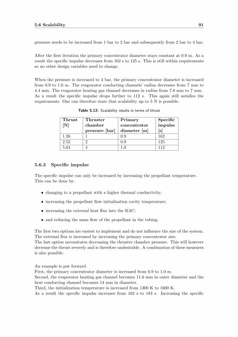
5.6 Scalability 91
pressure needs to be increased from 1 bar to 2 bar and subsequently from 2 bar to 4 bar.
After the first iteration the primary concentrator diameter stays constant at 0.9 m. As aresult the specific impulse decreases from 162 s to 125 s. This is still within requirementsso no other design variables need to change.
When the pressure is increased to 4 bar, the primary concentrator diameter is increasedfrom 0.9 to 1.0 m. The evaporator conducting channels’ radius decreases from 7 mm to4.4 mm. The evaporator heating gas channel decreases in radius from 7.8 mm to 7 mm.As a result the specific impulse drops further to 112 s. This again still satisfies therequirements. One can therefore state that scalability up to 5 N is possible.
Table 5.12: Scalability results in terms of thrust
Thrust[N]
Thrusterchamberpressure [bar]
Primaryconcentratordiameter [m]
Specificimpulse[s]
1.26 1 0.9 162
2.52 2 0.9 125
5.04 4 1.0 112
5.6.3 Specific impulse
The specific impulse can only be increased by increasing the propellant temperature.This can be done by:
• changing to a propellant with a higher thermal conductivity;
• increasing the propellant flow initialization cavity temperature;
• increasing the external heat flux into the RAC;
• and reducing the mass flow of the propellant in the tubing.
The first two options are easiest to implement and do not influence the size of the system.The external flux is increased by increasing the primary concentrator size.The last option necessitates decreasing the thruster chamber pressure. This will howeverdecrease the thrust severely and is therefore undesirable. A combination of these measuresis also possible.
An example is put forward.First, the primary concentrator diameter is increased from 0.9 to 1.0 m.Second, the evaporator heating gas channel becomes 11.6 mm in outer diameter and theheat conducting channel becomes 14 mm in diameter.Third, the initialization temperature is increased from 1300 K to 1600 K.As a result the specific impulse increases from 162 s to 183 s. Increasing the specific

92 Conceptual design
impulse further necessitates a more elaborate redesign for Concept 1. In particularthe interface between the RAC and evaporator will have to be altered; in the currentdesign the high initialization temperature will lead to a very high evaporator heating gastemperature.This is illustrated for Concept 2. The ’normal’ heating gas temperature for the conceptis around 980 K. Increasing the primary concentrator diameter to 1.8 m and increasingthe initialization temperature to 2000 K increases the heating gas temperature to 1280K. This in turn violates thresholds within the ORC.Scalability in terms of specific impulse is therefore limited.
5.7 Thermal stresses
Due to the large temperature increases of some of the thermal nodes and temperaturedifferences between adjacent nodes, significant thermal stresses could be generated withinthe system. Therefore one needs to know whether the system can cope with these stresses.
Assuming the nodes’ material is linearly elastic and isotropic, the thermal stress in normaldirection can be computed by equation 5.8 (Barron & Barron 2011).
σnormal =αte ·∆T · E
1− 2ν(5.8)
Here E is the Young’s modulus and ∆T is the temperature difference between the initialtemperature (assumed room temperature) and the temperature at a particular timeinstance. The variable αte is the material’s thermal expansion coefficient and ν is thematerial’s Poisson’s ratio.
In Table 5.13 the maximum thermal stresses for Node 3 to Node 9 are displayed. Theconcepts have been indicated by their RAC configuration and propellant for ease of use.
Table 5.13: Maximum thermal stresses for each concept’s thermal nodes in GPa
Node Con.1-Ammonia
Con. -Hydrogen
Cyl.2-Ammonia
Cyl. -Hydrogen
Spher.3-Ammonia
Spher. -Hydrogen
3 8 17 9 17 10 15
4 5 14 6 14 7 12
5 5E-1 5E-1 2E-1 3E-1 6E-4 1E-3
6 59 74 47 59 63 62
7 59 74 47 59 63 62
8 51 58 42 53 55 50
9 45 54 39 50 51 471 Con. = Conical RAC2 Cyl. = Cylindrical RAC3 Spher. = Spherical RAC
The largest thermal stresses in all concept occur in Node 6 and Node 7. This is to beexpected as these nodes reach the largest temperatures in the system. The yield stressfor molybdenum is 329 GPa. The largest stresses in the two nodes do not exceed this
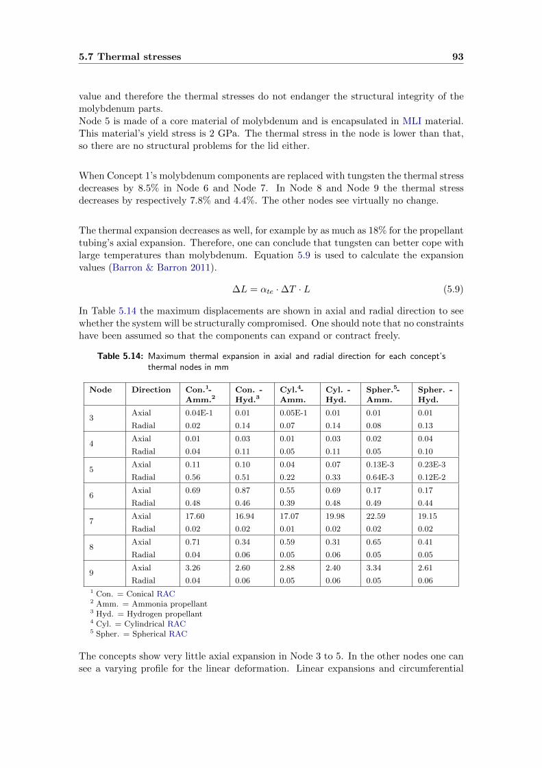
5.7 Thermal stresses 93
value and therefore the thermal stresses do not endanger the structural integrity of themolybdenum parts.Node 5 is made of a core material of molybdenum and is encapsulated in MLI material.This material’s yield stress is 2 GPa. The thermal stress in the node is lower than that,so there are no structural problems for the lid either.
When Concept 1’s molybdenum components are replaced with tungsten the thermal stressdecreases by 8.5% in Node 6 and Node 7. In Node 8 and Node 9 the thermal stressdecreases by respectively 7.8% and 4.4%. The other nodes see virtually no change.
The thermal expansion decreases as well, for example by as much as 18% for the propellanttubing’s axial expansion. Therefore, one can conclude that tungsten can better cope withlarge temperatures than molybdenum. Equation 5.9 is used to calculate the expansionvalues (Barron & Barron 2011).
∆L = αte ·∆T · L (5.9)
In Table 5.14 the maximum displacements are shown in axial and radial direction to seewhether the system will be structurally compromised. One should note that no constraintshave been assumed so that the components can expand or contract freely.
Table 5.14: Maximum thermal expansion in axial and radial direction for each concept’sthermal nodes in mm
Node Direction Con.1-Amm.2
Con. -Hyd.3
Cyl.4-Amm.
Cyl. -Hyd.
Spher.5-Amm.
Spher. -Hyd.
3Axial 0.04E-1 0.01 0.05E-1 0.01 0.01 0.01
Radial 0.02 0.14 0.07 0.14 0.08 0.13
4Axial 0.01 0.03 0.01 0.03 0.02 0.04
Radial 0.04 0.11 0.05 0.11 0.05 0.10
5Axial 0.11 0.10 0.04 0.07 0.13E-3 0.23E-3
Radial 0.56 0.51 0.22 0.33 0.64E-3 0.12E-2
6Axial 0.69 0.87 0.55 0.69 0.17 0.17
Radial 0.48 0.46 0.39 0.48 0.49 0.44
7Axial 17.60 16.94 17.07 19.98 22.59 19.15
Radial 0.02 0.02 0.01 0.02 0.02 0.02
8Axial 0.71 0.34 0.59 0.31 0.65 0.41
Radial 0.04 0.06 0.05 0.06 0.05 0.05
9Axial 3.26 2.60 2.88 2.40 3.34 2.61
Radial 0.04 0.06 0.05 0.06 0.05 0.061 Con. = Conical RAC2 Amm. = Ammonia propellant3 Hyd. = Hydrogen propellant4 Cyl. = Cylindrical RAC5 Spher. = Spherical RAC
The concepts show very little axial expansion in Node 3 to 5. In the other nodes one cansee a varying profile for the linear deformation. Linear expansions and circumferential

94 Conceptual design
expansions of more than 1 mm have to be specifically addressed. The latter is equal to aradial expansion of 0.16 mm.
All concepts feature a significant axial expansion of the propellant tubing. This requiresallowances when attaching this section of tubing to the rest of the propellant feed system.No other measures have to be taken as all expansions are 0.3-0.4% of the total tubinglength.
The axial expansion of the evaporator heating gas channel is less of a concern as theseare isolated from the rest of the system by the evaporator heat conducting channels. Thechannels themselves show less than 0.16 mm radial expansion which is acceptable. Thecavity radial expansion can be dealt with by employing a small allowance between thecavity insulation and the cavity itself or attaching constraints at the mounting points ofthe RAC. The same applies for the cavity lid.
5.8 Overall comparison of concepts
5.8.1 Performance
One can state that using liquid hydrogen produces a lighter system with the downside ofhaving a more voluminous system.In addition liquid hydrogen generates a substantially higher average specific impulsearound 650 s versus about 200 s for liquid ammonia. The resulting thrust however isslightly lower.Liquid hydrogen concepts also generate more system-specific impulse. Concept 1, 3 and 5on the other hand provide the highest total impulse in comparison with the other concepts.No clear winners can be discerned with respect to the size criterion as each concept variesin performance in terms of footprint and propellant tank volume. All concepts are capableof generating 100 W in power.
Judging by the inquiries concerning scalability and extrapolating from Concept 1 to theother concepts, the concepts can generate around 100 W without a significant enlargingof the system. A higher power output will require large passive condensers for the powersubsystem and a larger system as a whole.Along the same line of thought, thrust levels up to 5 N can be achieved for all conceptswithout violating Requirement 4.Scalability in terms of specific impulse is limited as large increases will require a significantredesign of each concept.
5.8.2 Thermal stresses and expansions
All the calculated thermal stresses are below the yield strengths of the components’materials.For Concept 1 to 4 thermal expansion measures are required for the cavity and cavity lid

5.9 Conceptual trade-off 95
as these nodes feature radial expansion of 0.2 to 0.6 mm.All concepts have to deal with the axial expansion of the propellant tubing with valuesup to 2 cm. This can be done through larger design allowances and constraints.
In Section 5.9 a trade-off will be made based on the discussed performance parameters toselect the concept which will be designed in more detail.
5.9 Conceptual trade-off
This thesis aims to synthesize a detailed design of a solar thermal hybrid system. Thereforea conceptual design must be selected which will be pursued further in the design process.This requires a trade-off of the six conceptual designs. This trade-off uses a classicalscheme. Before this trade-off can be made, some trade-off criteria need to be identified.
5.9.1 Trade-off criteria
The trade-off criteria are:
1. Specific impulse
2. System-specific impulse
3. Thrust
4. Wet system mass fraction
5. System volume
6. System complexity
One notes that power is absent even though it is a system requirement and KPP. It hasbeen omitted since all concepts have shown to satisfy the 100 W requirement and arecapable of scaling up the power output through a small change of design variables. Assuch there will not be a difference in the performance of the concepts in this regard.With the criteria defined, their relative importance needs to be addressed in the form ofweighting factors.
5.9.1.1 Weighting factors
To determine the weighting factors of each criterion the theory of Analytical HierarchyProcess (AHP) is applied (Saaty 1990). This theory states that the criteria must becompared with each other in terms of relative importance.Table 5.15 gives the resulting comparison matrix as defined in Equation 5.10 which

96 Conceptual design
represents this relative importance. The set of weighting factors is the associated eigenvectorv of the nxn comparison matrix as calculated in the Equation 5.11.
W =
w1w1
· · · w1wn
.... . .
...wnw1
· · · wnwn
(5.10)
(W − λI)v = 0 (5.11)
Table 5.15: Trade-off criteria comparison matrix
Criteria 1 2 3 4 5 6 Weighting factors
1 1 1/3 1 1/4 1/3 1/5 0.1012 3 1 2 1/2 1/3 1/4 0.1933 1 1/2 1 1/3 1/2 1/4 0.1254 4 2 3 1 2 1/4 0.3595 3 3 2 1/2 1 1/5 0.2766 5 4 4 4 5 1 0.855
Here, there are six criteria so n is 6. In addition the maximum and only non-zeroeigenvalue λ is 6.37.Equations 5.12 and 5.13 are used to calculate respectively the consistency index CI andthe consistency ratio CR.Tummala & Ling (1998) gives a comparison of different calculations of the randomconsistency index (RCI) and states that an RCI of 1.24 is accurate for an n of 6.
CI =λmax − nn− 1
(5.12)
CR =CI
RCI· 100% (5.13)
A consistency index and ratio of respectively 0.074 and 6% are determined. A matrixwith a ratio below 10% is considered consistent, so the calculated weighting factors areconfirmed to be acceptable.
5.9.1.2 System volume criterion
The performance of the concepts in all but the fifth criterion has already been determinedin Chapter 5. The preliminarily estimated system volume is considered a sum of thepropulsion subsystem length times its maximum diameter squared and the propellanttank volume as shown in Equation 5.14. The power subsystem is not taken into accountas its characteristics are as of yet unknown. Furthermore, its volume will stay constantno matter which concept is selected since each concept generates about the same amountof power.
Vsystem = Vtank + Lpropulsion · d2propulsion (5.14)
Table 5.16 for the system volume for each conceptual design.

5.9 Conceptual trade-off 97
Table 5.16: System volume estimate of concepts
Concept System volume [m3]
1 0.137
2 0.171
3 0.133
4 0.171
5 0.092
6 0.167
Since the propellant tank volume is dominant, it is no surprise that the concepts which useliquid ammonia have a substantially smaller system volume. Concept 5 has the smallestvolume whereas Concept 2 and 4 have the largest volume.
5.9.1.3 System complexity criterion
System complexity is a measure of how difficult it will be to manufacture, assemble andoperate the system. The geometry of the system naturally influences integration andmanufacturing. Sections which are symmetric and straight along the longitudinal axisare more advantageous in this regard.For example, a cylindrical cylinder and spiral tubing with the same spiral radius areeasier to manufacture than spherical chambers and spiral tubing with variable radii.Furthermore, fastening tubing to a cylindrical RAC is less intricate than fastening itto a spherical RAC. Therefore, in order of increased complexity the cylindrical, conicaland spherical are placed after each other.
In addition, the cryogenic propellant storage increases the complexity of the propellantstorage and feed subsystem considerably. The cryogenic storage temperature for hydrogenand ammonia are respectively 17 K and 243 K. Clearly ammonia can be kept at thattemperature more easily with less thermal control measures than hydrogen at its owntemperature.This is illustrated in Figure 5.57 which shows a simulated temperature profile for a Al-6061propellant tank for Concept 2. The MLI insulation around the tank is 4 cm thick. Here,only radiation and conduction to the spacecraft interior is taken into account. The interioris assumed to be a favorable 100.15 K.
One can see that even with such a low environment temperature the temperature of thetank increases from 17 K to 19 K after only 4.5 hours. Even within this short period oftime the increase in propellant tank temperature is large. Keeping temperatures low, letalone at 17 K, will require additional devices and additional system mass.Active coolers however increase the mass of the system substantially according to terBrake & Wiegerinck (2002). Passive cooling is therefore favorable as it usually entailsintegration of radiators in the existing spacecraft structure.
A test case for passive cooling of the propellant tank of Concept 2 is evaluated to checkfor feasibility. One assumes again an interior temperature of 100.15 K. Four copper

98 Conceptual design
Figure 5.57: Propellant tank temperature for Concept 2
conductors conduct heat to a carbon-carbon honeycomb radiator. It has an area of 2 m2,a thickness of 1 cm, a density of 1884 kg/m3, a thermal conductivity of 233.5 W/mK,a specific heat capacity of 687 J/kgK (Ohlhorst et al. 1997) and finally an emittance of0.91 due to the application of a silicone black paint coating (AZ Technology 2008).This yields Figure 5.58. The tank temperature increases from 17 K to 20.1 K in a 4.5 hour
Figure 5.58: Propellant tank temperature with passive radiator cooling
time frame with a slightly increasing temperature gradient at the end of the evaluatedperiod. Not only does the propellant tank temperature still exceed the 17-K requirement,the temperature increase has in fact worsened.Note that in this test case the single radiator is very large; if more than one propellanttank is required the design becomes even more challenging.Taking all the observations in this section into consideration, the concepts which useliquid hydrogen get a severe complexity penalty.
5.9.2 Trade-off and selection of final concept
Finally, before the concepts can be compared and traded-off, the score range must bedetermined to compare the concepts. To make differences between the concepts the most

5.9 Conceptual trade-off 99
clear, scores from 1-5 can be given for each criterion, ’5’ being the best in performanceand ’1’ being the worst. The weighting factors are taken from Section 5.9.1.1.In Table 5.17 the total score for each concept is given as well as the scores for eachcriterion.
Table 5.17: Concepts trade-off
Concept Specificimpulse
Systemspecificimpulse
Thrust Wetsystemmassfraction
Systemvolume
Systemcomplexity
Total
Weight 0.101 0.193 0.125 0.359 0.276 0.855
1 1 (0.101) 1 (0.193) 5 (0.625) 2 (0.718) 4 (1.104) 4 (3.44) 6.181
2 4 (0.404) 4 (0.772) 4 (0.500) 4 (1.436) 2 (0.552) 1 (0.855) 4.519
3 2 (0.202) 1 (0.193) 5 (0.625) 2 (0.718) 4 (1.104) 5 (4.275) 7.117
4 4 (0.404) 3 (0.579) 4 (0.500) 3 (1.077) 2 (0.552) 1 (0.855) 3.967
5 3 (0.303) 3 (0.579) 5 (0.625) 3 (1.077) 5 (1.380) 2 (1.710) 5.674
6 5 (0.505) 5 (0.965) 4 (0.500) 5 (1.795) 3 (0.828) 1 (0.855) 5.448
The final sum of scores yields two concepts with a high score, namely Concept 1 and 3.Looking at Section 5.9.1.3 the system complexity and difficulties of integrating the sphericalRACs and, in the case of Concept 6, cryogenic systems in the small spacecraft bus, makeConcept 5 and 6 less desirable.Concept 1 differs slightly with Concept 3 as it has a more complex geometry and lessspecific impulse, having respectively an impact on system assembly and performancescalability. Concept 3 is therefore the preferred concept.It has a relatively low system complexity, a high thrust and a low system volume estimate.Its main disadvantage is the low system-specific impulse meaning more system mass willbe required to generate a certain amount of impulse.
Chapter 6 will discuss Concept 3 and its detailed design further.

100 Conceptual design
Chapter 6
Detailed design
In Chapter 5.9 Concept 3 was selected to be designed in more detail.First, the chapter will discuss the secondary concentrator and its casing. Subsequentlythe pre-cavity chamber will be shortly described. Afterwards the mounting and designof the cylindrical RAC and its lid will be detailed. The propellant tubing and propellantfeed system are thereafter discussed, followed by the interface with the evaporator.Additionally, the thruster design is detailed.Finally, the chapter concludes with the subsystem integration.
6.1 System architecture and design options
This section will detail the overall system architecture and the design options for each ofthe system components.In Figure 6.1 the hybrid system architecture can be seen. For the components withinthe power and propulsion subsystems different design options have been given. Thered options have been discarded whereas the green options have been selected in theconceptual design phase.
The primary concentrator can be on-axis or off-axis with respective to the RAC. Sincean on-axis concentrator requires a less complex deployment and pointing mechanism theon-axis option is selected for this design. According to Nakamura et al. (2004) the off-axisconcentrator however has been previously estimated to be lighter.
In Wong & Macosko (1999) the refractive secondary concentrator’s advantages over areflective one have been presented. In terms of throughput efficiency and concentrationratio the reflective concentrator has worse performance than the refractive concentrator.The refractive secondary concentrator is therefore selected and the concentrator in questionis made of a single-crystal sapphire material.
In Chapter 5 conical, cylindrical and spherical RACs were analyzed and compared. Theselected cylindrical RAC for Concept 3 is further developed.
101

102 Detailed design
Figure 6.1: System architecture and design options
The propellant feed system features a number of design choices. Only the tubing configurationhas been predetermined in Section 5.2.4, namely spiral propellant tubing.
6.2 Propulsion subsystem
6.2.1 Functional and physical architecture
Looking at Figure 2.1 one can get an idea of the functionalities of the propulsion subsystem.The functionalities can be visualized by a socalled Hatley-Pirbhai diagram which showsthe system inputs and outputs with the intermediate processes.In this diagram the propellant flow has been engaged as the sun sensor has verified thatthe spacecraft is in the daylight phase of its orbit.In case enough thrust has been provided and the RAC and propellant tubing temperaturesexceed the operational constraints, respectively the propellant flow is deactivated and theprimary concentrator pointing mechanism is directed to reposition the concentrator.
By matching this diagram with the physical architecture in Figure 6.3, the latter can beverified so as not to omit any components.The sun sensor will not be included in the detailed design as this device will also be partof the ADCS and small micro-electro-mechanical systems (MEMS) sun sensors are easilyavailable, therefore not compromising feasibility.

6.2 Propulsion subsystem 103
The propellant tank will have MLI, but may also include additional thermal controlmeasures. See Section 6.2.5.4 for further discussion on this topic.
Figure 6.2: Hatley-Pirbhai diagram for propulsion subsystem
Figure 6.3: Propulsion subsystem physical architecture

104 Detailed design
6.2.2 Secondary concentrator
The refractive secondary concentrator serves to decrease the pointing requirements forthe primary concentrator as the solar image from the primary concentrator is furtherdecreased in size. Its lens is made of a single-crystal sapphire material. A 2.5-cm-diametersingle-crystal sapphire lens with a focal length of 5 cm was found to be easily procurable(Edmund Optics 2014).
6.2.2.1 Concentrator lens
The bond between the lens and concentrator casing needs to be sufficiently rigid andcapable of handling large temperature differences so that the focusing ability of the lens isnot compromised during its service life. To fasten the lens to the casing a high-temperatureadhesive is applied to the side of the lens. The casing is made of two half-cylinders andmade to close around the circumference of the sapphire lens after which the adhesivestrengthens the permanent bond.In the event that there has to be some reversibility in the system integration process, theadhesive has to be omitted. In order to achieve the same level of fastening and circumventlens jitter a high-temperature silicone rubber O-ring can be placed between the casingand the lens. The fastening of the two half-cylinders in that case is done by bolts throughintegrated flanges. This also requires a small allowance between the casing and lens forthe O-ring and for the thermal expansion of the lens.The thermal expansion in the plane of the lens according to Kyocera (2013) is 7.5·10−6
K−1 at the maximum temperature of 486 K (see Figure 5.28).
This results in a radial expansion of 0.03 mm according to Equation 5.9. This is anincrease of 0.2%. The decrease of the focal length due to thermal expansion will also besmall, in the order of several microns (O’Shea et al. 2004). Wong et al. (2000) and Wong(2000) do not mention significant concentration ratio differences during high-temperaturetests.Concluding the allowance for thermal expansion can be very small. An allowance of 1 mmshould therefore be sufficient to assemble the parts and leave room for thermal expansion.
To limit the temperature of the lens during multiple heating cycles, 15 thermal straps areattached to the outer extremities of the lens.The thermal straps feed-through holes in the concentrator casing and interface with heatsinks within the interior of the spacecraft, assumed to be at a temperature of 293.15 K.A length of 15 cm is assumed behind the feed-through holes per thermal strap. Thesethermal straps have a mass of 77 g, a thickness of 3.6 mm and a conductance of 0.82 W/K(Thermacore 2014). They have a custom width of 5 mm.This yields a thermal conductivity of 9247 W/mK according to Equation 6.1 which isderived from Pouillet’s law. This law expresses electrical resistance as a function ofelectrical resistivity which are respectively reciprocal to thermal conductance and thermalconductivity.
κ =G · LA
(6.1)

6.2 Propulsion subsystem 105
Here, κ is the thermal conductivity and G is the thermal conductance.
The total thermal strap mass estimate is 1.155 kg. The secondary concentrator and itscasing are respectively 0.008 kg and 0.638 kg.In Figure 6.4 the resulting temperature plot can be seen. Comparing this plot to Figure5.28 shows that the lens maximum temperature in the third orbit has decreased from 486K to 362 K.
Figure 6.4: Temperature profile for Concept 3 with 15 thermal straps attached to thesecondary concentrator lens
6.2.2.2 Concentrator casing
The casing is made of two molybdenum half-cylinders with a length of 4.3 mm, an innerradius of 18 mm and a width of 53 mm.The inner radius has been determined taking into account the spacing of 1 mm betweenthe edge of the concentrator lens and the casing as detailed in the previous section.The two parts can be fastened together by including a small baffle on one side of each partalong its entire length. The application of some bolts and nuts will facilitate the fastening.Note that these mechanical fasteners need to withstand mechanical and acoustic loadsduring launch. The casing is surrounded by MLI.The front of the casing faces space and is therefore coated with a white-paint coating tolimit its temperature. The casing frontal surface itself is bolted to the exterior of thespacecraft as well as to some attachment points inside the spacecraft bus.In Figure 6.5 a schematic is given for the concentrator and its casing.

106 Detailed design
Figure 6.5: Schematic for secondary concentrator assembly
6.2.3 Pre-cavity chamber
The pre-cavity chamber connects the secondary concentrator and its casing with the RAClid and prevents radiation from spreading to the rest of the spacecraft interior.It is a molybdenum cylinder with a 10.8 mm wall thickness with about the length of thesecondary concentrator focal length and an interior coating of white paint. The coating isapplied to limit solar absorptance in the event misalignment of the primary concentratorleads to solar radiation falling on the chamber interior surface. Its exterior is coveredwith MLI to prevent heat from leaking into the interior of the spacecraft.The cylinder attaches to the RAC lid and secondary concentrator casing through mechanicalfastening of their flanges (Figure 6.6).
Conductive tape with a grounding strap can be used to ground the MLI. Hook-and-pilefasteners can fasten the insulation to the metal substrate by tightening the insulationmaterial around the chamber. The fasteners themselves can be attached by adhesives orriveting (Finckenor & Dooling 1999). The chamber itself has a mass of 2.022 kg.
6.2.4 RAC and RAC lid
One of the most important components in the hybrid system is the RAC.The RAC lid has a 10.5-cm wide aperture to allow the incoming solar flux to heat thecavity. The surroundings of the cylindrical RAC and its lid are insulated with MLI,except for some cut-outs for attached components. The insulation is applied as a shellsurrounding the cavity and propellant tubing.

6.2 Propulsion subsystem 107
Figure 6.6: Schematic for pre-cavity chamber assembly
The lid is considered a separate component as it is mounted separately from the cavity. Itscore structure is made of molybdenum which is encompassed by MLI to achieve sufficientinsulating performance. The molybdenum serves to limit the thermal expansion of thelid. The thickness of the molybdenum core is 14 mm. On both sides a 43-mm thick MLIblanket has been attached to the core.There is a 1 mm small spacing between the RAC and lid to allow for some thermalexpansion of the RAC.Summing up the insulation and the core material, the lid has a mass of 0.987 kg.
The RAC is a cylinder as has already been determined. In the model a wall thickness of10.8 mm is calculated as explained in Section 5.1.2. On the inside it has a black paintcoating for the best absorptive properties. It is open-ended on one side whereas the rearof the cavity is closed. The cavity itself is mounted to a surrounding frame with mountingpoints to the rest of the spacecraft and attachment points for insulation.There are different options for mounting the RAC to the frame. Two distinctive mountingcategories have been given in Figure 6.1. Three specific options are evaluated:
1. PODS attached to both the frame and the RAC
2. Aluminium struts attached to both the frame and the RAC
3. Clamping of the RAC within the frame by using a large amount of MLI andhook-and-pile fasteners
During the evaluation of the different options a spacing between the frame and the top ofthe propellant tubing of 10 cm is assumed. The sink temperature has been set at 293.15K. The options are detailed in Section 6.2.4.1 to Section 6.2.4.3.

108 Detailed design
6.2.4.1 PODS
First of all, the PODS option is analyzed. (Plachta et al. 2006) gives more informationconcerning these devices. In this case their core is made of a graphite epoxy composite.Their function is to limit heat transfer by limiting the cross-sectional area through whichheat can be transferred and by having a low thermal conductivity. This in turn limitsthe decrease of temperature of the RAC. In Figure 6.7 a schematic is provided for thesedevices.
Figure 6.7: Schematic for PODS (Plachta et al. 2006)
The size of the PODS is determined by the mass of the RAC. Since it is only 18.7 kgwithout support structures, no large struts are required. Using Hopkins & Payne (1987)one can calculate a preliminary calculation of PODS dimensions. In this calculation thepaper states a limit load of 10g in any direction and a maximum safety factor of 1.8.Equation 6.2 is a rudimentary calculation of the critical loads for these PODS. It yieldsa load of 3302 N. The outer tube wall thickness for the struts is calculated with Equation6.3 and results in a thickness of 0.181 mm.
Fcritical = MRAC · 10 · 9.81 · fsafety (6.2)
tPODS =
√Fcritical0.942E
(6.3)
RPODS =
(FcriticalL
2
π3E · tPODS
)1/3
(6.4)
Here, Fcritical is the critical load, RPODS is the PODS minimum tube radius and tPODS isthe PODS outer tube wall thickness. The variable fsafety is the safety factor and E is themodulus of elasticity for the graphite epoxy which is 106869 MPa according to Hopkins& Payne (1987). In addition, a thermal conductivity of 3.5 W/mK for graphite epoxycomposites has been stated.
Assuming a length of 10 cm for each PODS, the outer tube diameter becomes 7.6 mm.To estimate the mass of each PODS, it is considered a solid rod made of only graphitefibers. The density is assumed to be 1772 kg/m3 (Armanios 1997, p. 71). This yields a
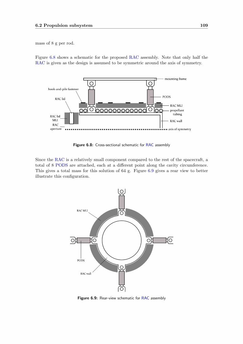
6.2 Propulsion subsystem 109
mass of 8 g per rod.
Figure 6.8 shows a schematic for the proposed RAC assembly. Note that only half theRAC is given as the design is assumed to be symmetric around the axis of symmetry.
Figure 6.8: Cross-sectional schematic for RAC assembly
Since the RAC is a relatively small component compared to the rest of the spacecraft, atotal of 8 PODS are attached, each at a different point along the cavity circumference.This gives a total mass for this solution of 64 g. Figure 6.9 gives a rear view to betterillustrate this configuration.
Figure 6.9: Rear-view schematic for RAC assembly

110 Detailed design
The model is run with 4 PODS at the front and 4 at the rear of the cavity. The RACmaximum temperature in the last evaluated orbit is calculated to be 12 K lower at 1368K than in the case without PODS as can be seen in Figure 6.10. This is a decrease of0.9% which is acceptable. The specific impulse as a consequence decreases by only onesecond to 180 s.
Figure 6.10: Temperature profile for Concept 3 with PODS
6.2.4.2 Aluminium struts
Aluminium struts are solid rods which have attachment points at the frame and at thecavity. To compare them with the PODS they too must cope with a launch load of 3302N.The Al 6061-T6 material in question has a density of 2700 kg/m3, a thermal conductivityof 167 W/mK and a tensile yield strength of 276 MPa (ASM Aerospace SpecificationMetals Inc. 2014).A solid rod with a diameter of 7.6 mm which needs to cope with 3302 N suffers a normalstress of 73 MPa which does not exceed the previously defined yield strength. The massof such a rod is 12.2 g. Eight of these aluminium rods give a total mass of 98 g.
In Figure 6.11 one can see the effect of having the RAC transferring heat through thealuminium rods. Comparing the figure to Figure 5.28 gives one a sense of the thermaldisturbances caused by the struts. The third orbit maximum cavity temperature decreasesfrom 1380 K to 1025 K. As a consequence the specific impulse at the end of the evaluatedperiod decreases from 181 s to 148 s.

6.2 Propulsion subsystem 111
Figure 6.11: Temperature profile for Concept 3 with Al 6061-rods between mounting frameand RAC
6.2.4.3 MLI and fasteners
Johnson & Fesmire (2011) gives a thermal conductivity of 0.1 mW/mK and a density of45 kg/m3 for the MLI material. If the 10-cm spacing needs to be completely filled withMLI one comes to a maximum of 0.0143 m3 insulation. This gives a mass of 0.645 kg. Thefastener mass cannot be defined without detailed knowledge of the number of fastenersand is therefore not taken into account. Even without this value however it becomes clearthat this option represents a larger mass increase than the other two options.
A 10-cm MLI blanket can have 100 aluminized Mylar layers if one extrapolates from(Johnson & Fesmire 2011). According to (Larson & Wertz 2005, p. 438) the effectiveemittance then drops to merely 0.00025. In Figure 6.12 one can see the resulting temperatureprofile for the propulsion subsystem.The MLI surrounding the RAC increases in thickness from 4.3 cm to 10 cm so it does notcome as a surprise that the maximum RAC temperature increases as less heat is allowedto dissipate from the cavity. In the third orbit this temperature increases from 1380 K to1381 K. The specific impulse increases by one second to 182 s.
6.2.4.4 Comparison of mounting options
Comparing the three options it becomes clear that the last option is the heaviest, butalso preserves the RAC temperature the best. The PODS option has the least mass andachieves virtually no temperature change with respect to the initial conceptual design.

112 Detailed design
Figure 6.12: Temperature profile for Concept 3 with 10-cm thick MLI around RAC
Furthermore, additional insulation can be applied at other locations around the cavityto further decrease heat dissipation, thereby mimicking the thermal control ability of thelast option.Concluding, in order to save mass, the first option is selected.
6.2.4.5 Mass budget
In Table 6.1 the mass budget for this part of the system is given.An MLI blanket of 43-mm thickness is still wrapped around the RAC and is taken intoaccount in the mass budget. This yields a mass for the RAC of almost 19 kg. Summingup all the different components a total mass of 24.8 kg is computed for the RAC system.

6.2 Propulsion subsystem 113
Table 6.1: Mass budget for RAC system
Component Mass [kg]
Primary concentrator 0.94
Secondary concentrator 0.01
Secondary concentrator casing 0.64
Thermal straps 1.16
Pre-cavity chamber 2.02
RAC lid incl. MLI 0.99
RAC incl. MLI 18.96
PODS 0.06
Total 24.78
6.2.5 Propellant feed system
The propellant feed system performs the physical transportation of the propellant fromthe propellant tank along the RAC to the thruster chamber. Figure 6.1 gives two differentregimes for achieving propellant flow, namely pump-driven and blow-down schemes:
• Pump-driven An electric (micro)pump forces the flow down-line. This requires inputpower, but there is accurate active control of the propellant flow.
• Blow-down The propellant is pressurized with a pressurant gas within the propellanttank and a valve down-line of the tank controls the propellant flow. Regulation by thevalve will guarantee that the correct tank outlet pressure is maintained independent ofhow much propellant is expelled out of the tank. The pressurant gas and propellantcan be optionally separated by a membrane. There is less control of the flow butvirtually no power is required.
The propellant tank itself is small as well as the amount of required propellant. Thereforea blow-down system should not be difficult to achieve.A major disadvantage of blow-down systems is that they typically increase the mass ofthe propellant tank as its thickness must increase to accommodate the larger internalpressure.In addition the ullage volume must be filled up with pressurant gas. A separate pressurantgas tank can also be considered although the small spacecraft bus volume imposes someconstraints for integration.A pump-fed system requires relatively heavy and large pumps with a large numberof moving parts, therefore increasing the mass of the spacecraft and reducing systemreliability. This makes the system unsuitable for small low-thrust propulsion systems.Taking all these advantages and disadvantages together, it becomes clear that for a smallsystem the blow-down option is the most advantageous.
One is reminded that liquid ammonia is used as propellant. The pressurant gas forthe liquid ammonia will be helium as ammonia has a higher boiling point than helium,meaning that at the cryogenic storage temperature helium is in a gaseous state.

114 Detailed design
In order to design the propellant feed system one needs to work from the back to the frontof the feed system. Hence, the thruster is the first component to be discussed. Afterwardsthe propellant tubing and the propellant tank are detailed.
6.2.5.1 Thruster
The thruster encompasses the thruster chamber and the nozzle. It is made of molybdenumto cope with the high-temperature exhaust gases. The thruster in question falls withinthe small thruster category with a chamber radius of 1 cm, a chamber length of 4 cm anda throat radius of 1.5 mm. The chamber pressure is set at 1.0 bar.To elaborate on the discussion in Section 5.2.3 twelve different bell-shaped nozzles arecompared. The length of each set of three nozzles is set at respectively 6, 7, 8 and 9 cm.The expansion ratio for each set of nozzles is set at 150, 225 and 300 which yields a nozzleexhaust diameter of respectively 3.67 cm, 4.50 cm and 5.20 cm.Table 6.2 gives the accompanying angles. The nozzle throat convergence half angle is 25degrees for all nozzles.
Table 6.2: Final comparison of nozzle shapes
Nozzle length[cm]/ Exhaustdiameter [cm]
Nozzle throatdivergence halfangle [deg]
Nozzle exhaustdivergence halfangle [deg]
Specificimpulse[s]
Thrust[N]
6/3.67 45 14.5 184 1.242
7/3.67 40 11.5 184 1.254
8/3.67 35 9.7 184 1.271
9/3.67 30 8.5 184 1.289
6/4.50 45 19.0 185 1.271
7/4.50 40 15.2 185 1.277
8/4.50 35 12.8 185 1.289
9/4.50 30 11.2 185 1.303
6/5.20 45 22.5 185 1.29
7/5.20 40 18.5 185 1.294
8/5.20 35 15.8 185 1.304
9/5.20 30 13.8 185 1.315
In Figure 6.13 the nozzle length-exhaust diameter ratio has been plotted against thegenerated thrust. One can see that for every expansion ratio there is a separate curve. Thethrust increases with a larger expansion ratio as well as with a larger nozzle length-exhaustdiameter ratio. There is virtually no change in the specific impulse.As can be seen in the figure, an expansion ratio of 300 and a nozzle length of 9 cm areselected to maximize thrust. The nozzle’s divergent section is situated just outside theexterior of the spacecraft on the opposite side of the side which features the primaryconcentrator. The thruster chamber itself is mechanically fastened to the exterior of thespacecraft.
As molybdenum has a high maximum operating temperature no thruster cooling isrequired. The flow effective exhaust velocity is 1.85 km/s. The mass flow at that point is732 mg/s.

6.2 Propulsion subsystem 115
Figure 6.13: Nozzle length-exhaust diameter ratio versus thrust
The mass of the chamber and nozzle itself is estimated by assuming that the chamberis an open-ended cylinder and the nozzle is formed by two hollow cones. The thrusterthickness is assumed 1 mm. This yields a thruster mass of 0.064 kg. The final requiredpropellant mass becomes 29.3 kg.
6.2.5.2 Propellant tubing
The molybdenum spiral propellant tubing has a thickness of 0.625 mm and an innerdiameter of 3.75 cm.This thickness has been calculated by assuming a certain diameter-thickness ratio basedon parts procurement data (Section 5.1.2).To calculate the pressure within the propellant tank in Section 6.2.5.3 the total pressureloss has to be determined. Looking at equation 3.62 the total tubing length and the flowconditions in the tubing need to be known to calculate the pressure loss.Below the three distinguishable feed lines are identified. The spiral tubing includes the8% reduction as described in Section 3.2.3.1.There are three feed lines:
• One from the cavity to the thruster chamber;
• One section of RAC-adjacent spiral tubing;
• One from the cavity to the propellant tank
LtubingRAC−thruster = 1− Lsystem − Lnozzle − Lchamber (6.5)
Ltubingtank−RAC1= 0.5−Rtank − Ltank/2− xfront−RAC (6.6)
Ltubingtank−RAC2= 0.5−RRAC −Rtank − tins − ttank (6.7)
Ltubingtank−RACtotal =(Ltubingtank−RAC1
+ Ltubingtank−RAC2
)· 1.1 (6.8)

116 Detailed design
The length of the RAC-adjacent tubing has already been calculated based on the numberof turns and the RAC size. This yields a length of 8.471 m.
The feed line from the RAC to the thruster is calculated by taking the entire width ofthe spacecraft bus of 1 m and subtracting the length of the system, the nozzle and thethruster chamber as seen in Equation 6.5. These are respectively 45.5 cm, 9 cm and 4cm. The assumption is made that the system is coaxial with one of the axes of symmetryof the spacecraft. This yields a length for this feed line of 41.5 cm.
The third feed line length depends on the position of the propellant tank within thespacecraft bus. The propellant tank is placed above the RAC to limit the complexity ofthe feed line. Furthermore by concentrating the propellant mass as much at the centerof the spacecraft as possible the spacecraft’s stability will be increased. This in turn willcause less attitude disturbances due to propellant sloshing. A 10% margin is included inthis feed line for bends.In equations 6.6 to 6.8 the length of this feed line is calculated. The length for this feedline then becomes 14 cm. Here, xfront−RAC is the location of the front of the RAC withrespect to the bus side wall. The variables tins and ttank are the thicknesses of the RACinsulation and the RAC wall.Figure 6.14 gives an illustration of the geometry involved. Summing the three tubing
Figure 6.14: Schematic for propellant tubing from propellant tank to RAC
lengths up yields a total tubing length of 9.14 m. This results in a tubing mass of 0.914 kg.
The pressure losses in the tubing can be compartmentalized in four different parts.
• Friction pressure losses when the propellant is in a liquid state
• Friction pressure losses when the propellant is in a gaseous state
• Friction pressure losses when the propellant is in a two-phase state

6.2 Propulsion subsystem 117
• Acceleration pressure losses due to the vaporization of the propellant
6.2.5.2.1 Pressure loss for liquid propellantThe liquid ammonia propellant is present from the tank to the RAC as it is stored as aliquid.The assumption is that the propellant will change phase in the first third section of theRAC propellant tubing. This assumption also means that only in the first sub-node ofnode 7 will the propellant temperature be decreased due to the latent heat. This heat isrequired to vaporize the propellant.Equation 3.49 shows that indeed the temperature decreases, since less convective heat isput into heating the propellant.
The pressure loss in bends is taken into account here as bends will be present within thetubing from the propellant tank to the RAC where the propellant is still in a liquid state.Figure 6.14 shows two bends. An additional third bend can be defined at the start ofthe spiral tubing. The radii of the 90 bends are assumed to be two times the tubingdiameter.Idel’chik (1986) gives equations to calculate the pressure loss in bends δpbend which isdefined in Equation 6.11. The pressure loss coefficient ξ which is required, is determinedaccording to Equation 6.10. The liquid flow Reynolds number is 538 and thereforeEquation 6.9 applies to calculate the loss scaling factor λ.
λ =20
Re0.65
(Dinner−tubing
2Rbend
)0.175
(6.9)
ξ = 0.0175λ
(Rbend
Dinner−tubing
)δbend (6.10)
δpbend =ξρpropU
2prop
2(6.11)
Here, Rbend is the bend radius and δbend is the bend angle in degrees.A loss coefficient of 0.83 is calculated. The pressure loss per bend is calculated to be 0.93Pa. This yields a total pressure loss in the bends of 2.8 Pa.Equation 3.62 is used to calculate the friction loss in the straight tubing sections whichyields 4.6 Pa.Therefore a total pressure loss of 7.4 Pa in the liquid state has to be taken into account.
6.2.5.2.2 Pressure loss for gaseous propellantThe gaseous ammonia is present in two-thirds of the RAC tubing and in the tubing fromthe RAC to the thruster.The spiral tubing can be represented by twenty 360 bends. As two-thirds of the spiraltubing features the gaseous flow only fourteen bends will be used to calculate the totalloss in the bends.The inner radius of the tubing is 2.35 mm and the bend radius is 71 mm. The mean flowproperties are applied to calculate the pressure loss (Equation 6.11).With a mean Reynolds number of 2.07·104 λ becomes approximately 0.045 (Idel’chik 1986,

118 Detailed design
p. 210).
This yields a pressure loss in each bend of 1.25 kPa and therefore a total bend loss in theRAC of 17.5 kPa.Equation 3.62 calculates the friction pressure loss along the two-thirds length of the spiraltubing. This results in a pressure loss of 85.6 kPa.Finally, the pressure loss in the tubing from RAC to the thruster chamber is calculated.The density of the propellant when it runs from RAC to the thruster is based on the idealgas law and the mean propellant temperature during propellant flow. Equation 3.62 isapplied here as well. The resulting friction pressure loss is only 9.3 kPa.This yields a total pressure loss in the gaseous state of 112.4 kPa.
6.2.5.2.3 Two-phase propellant and acceleration pressure lossesWhen calculating the two-phase friction loss in one third of the spiral tubing, the assumptionis made that half the propellant flow is in the liquid phase and half in the vapor phase.The surface tension for liquid ammonia at 240 K is 33.9·10−3 N/m. The Baker parametersBx and By are respectively 0.93 and 2.81·104. From Figure 3.9 this yields an annulartwo-phase flow in the tubing and the following correlation for the unit loss φ.
McKetta Jr. (1992) gives Equation 6.12 for the unit loss in an annular flow.D is the inner diameter of the pipe in inches. L is the tubing length in feet.Equation 6.13 calculates the actual pressure loss based on the friction loss when the entireflow in the section is evaporated. The friction loss δpvapor has been calculated using meangaseous flow conditions. Finally, a two-phase pressure loss of 12.6 kPa is calculated.
φ = aXb (6.12)
a = 4.8− 0.3125D
b = 0.343− 0.021D
X =√
(Wl/Wv)1.8 · (ρv/ρl) · (µl/µv)0.2
δp = δpvaporφ2 · L/100 (6.13)
Equation 3.67 computes the pressure losses due to the expansion of the propellant as aresult of evaporation. As the volume of the propellant increases, a pressure loss in thepropellant occurs which needs to be compensated. This acceleration pressure loss has avalue of 3 kPa.
6.2.5.2.4 Total pressure lossIn Table 6.3 the pressure losses are summed up according to Equation 3.68.
Clearly, the gas-phase friction pressure losses are most severe, mainly due to the largefeed line length and the high flow velocity of the gaseous propellant. The total pressureloss amounts to 1.28 bar. With a chamber pressure of 1 bar, the tank pressure at thetotal evacuation of the tank must therefore be 2.28 bar.

6.2 Propulsion subsystem 119
Table 6.3: Pressure losses
Pressure loss Value [kPa]
Friction pressure loss - liquid-phase 7.4E-3
Friction pressure loss - gas-phase 112.4
Friction pressure loss - two-phase 12.6
Acceleration pressure loss 3.0
Total pressure loss 128.0
The spiral propellant tubing is fastened on the outside of the cavity. This fastening hasto be performed adequately as during launch high-frequency vibrations could cause largeexcitations in this part of the system.At the beginning and end of the tubing, two 2 cm wide titanium-alloy rings are clampedaround the tubing as seen in Figure 6.15. The clamping locations are also fastened to theframe. A titanium-alloy has been chosen to prevent large heat dissipation as the materialcan have a thermal conductivity as low as 4.8 W/mK (AZO Materials 2014).
Figure 6.15: Schematic for propellant tubing fasteners
The end points of the RAC tubing are threaded so that feed lines from the propellanttank and to the thruster can be independently mounted.

120 Detailed design
6.2.5.3 Propellant tank
The system volume estimate is a sum of the volume estimate for the RAC and for thepropellant tank as these are the two major components contributing to the system volume.The propellant tank takes up more than half of the system volume estimate, namely 0.052m3 out of a total volume of 0.08 m3.If a spherical tank is adopted, it must have an inner diameter of 46 cm. This leads to alimited remaining volume within the spacecraft bus. Therefore to conserve practical spacewithin the bus, a cylindrical tank with hemispherical end-caps will be adopted instead ofa spherical tank.After a number of iterations one single tank was deemed feasible with an inner radius of17.6 cm and a length of 30 cm excluding the end-caps. The total (inner) length of thetank becomes 65.2 cm which fits easily inside the spacecraft bus and leaves room for afeed line and insulation.Passive and/or active thermal control can be used to keep the propellant tank and itscontents at a cryogenic temperature of 240 K. See the subsequent paragraphs for moredetails.
As seen in Section 6.2.5.2 the pressure at the flow control valve behind the tank needs tobe 2.28 bar. Recall that 80% of the tank volume is propellant and 20% is ullage which isfilled with helium pressurant gas.
PV
T= c (6.14)
Taking the combined gas law in Equation 6.14 and assuming a constant temperaturewithin the propellant tank, the product of pressure and volume stays constant. Thisyields the following equation:
ptankmax =ptanknominalVtank
0.2Vtank(6.15)
A maximum pressure of 11.4 bar is calculated for the helium pressurant so that the 2.28bar propellant pressure is still achieved at total evacuation of the propellant tank.With a pressure loss of 1.28 bar the chamber pressure of 1 bar is then maintained.Since a higher pressure will result in a higher boiling point temperature (Equation 6.14)no changes to the propellant storage temperature are necessary. Using the ideal gas lawfor computing the density of the helium yields a pressurant gas mass of 23.2 g.
The maximum pressure requires a certain thickness of the propellant tank shell. Theselected propellant tank material is Al 6061-T6, an aluminium alloy, which has a lowdensity of 2700 kg/m(3), a thermal conductivity of 167 W/mK and a yield strength of276 MPa (ASM Aerospace Specification Metals Inc. 2014).From Swearengen (1972) one knows that the aluminium alloy yield strength in thetemperature range 200 K to 350 K is independent of material temperature. No temperature-dependentcorrections in the tank thickness therefore need to take place.Liquid ammonia is non-corrosive and therefore no corrosion allowance is applied whencalculating the minimum design thickness for the tank shell.

6.2 Propulsion subsystem 121
The maximum of the results from solving Equation 6.17 and 6.16 is considered theminimum thickness. The longitudinal yield strength and the circumferential yield strengthare considered equal as the material is considered isotropic. These equations have beenderived from ASME (2013).
σyieldcirc =pmax · (Rtank + 0.6ttank)
ttank(6.16)
σyieldlong =pmax · (Rtank − 0.4ttank)
2ttank(6.17)
Here, Rtank is the tank internal radius and ttank is the tank shell thickness.A minimum tank wall thickness of 1.1 mm is calculated with a safety factor of 1.5.
σnormal = Faxial/Acs (6.18)
Equating Equation 6.18 to the yield strength of the tank material, yields a minimum wallthickness. The axial loading Faxial of 5.4 kN is calculated according to Equation 6.2;instead however the mass considered is the sum of the masses of the tank, the propellantand the pressurant gas. The safety factor stays 1.8. This yields a minimum thickness of0.02 mm. As one can see the minimum tank wall thickness causes no problems for axialloading.As the surface area of the propellant tank is 0.72 m2 this yields an estimate of the totaltank mass of 2.10 kg. Together with the propellant and pressurant gas a total propellanttank mass of 31.4 kg is determined.
6.2.5.4 Propellant tank thermal control
In Figure 6.1 passive and active thermal control options are discerned. Passive control hasthe advantage that it does not require power. The thermal control ability is constrainedhowever. Active control requires heavy and relatively complex components, but achieveslarger cryogenic cooling. The following solutions are available:
• Passive thermal control:
– MLI
– Surface coatings
– Radiators
– Optical Solar Reflectors (OSR)
• Active thermal control:
– Heat pipes
– Thermal control louvers
– Electric heaters
– Thermoelectric coolers

122 Detailed design
Since the spacecraft bus is small and there is already a significant amount of tubing withinthe spacecraft, a heat pipe system is considered too troublesome to integrate.Thermoelectric coolers are heavy and require large amounts of power. For example inZhang et al. (2007) a pulse-tube cooler achieves 10 W of cooling power by supplying 190W of electrical power. According to the review by (ter Brake & Wiegerinck 2002) thiscooler would be in the mass range of 8-9 kg. Therefore these coolers will not be usedhere.Electric path heaters however are small Kapton-film heaters which can be attached inlarge numbers to heat certain surfaces. They also use relatively little power.Thermal control louvers consist of blades which can open and close and can thereforeprevent or encourage a heat flux being transferred across it. They are actuated throughthermally sensitive springs and can reject six times as much heat in an open state thanin a closed state (Larson & Wertz 2005, p. 442).
In terms of the passive thermal control options, OSRs are used on the surface of space-facingstructures and components. Since they have a high emittance and low absorptance, theyare very good at keeping surfaces cool, even when the surfaces are illuminated by Earthalbedo and direct sunlight.Radiator panels are also used as a thermal control interface with the external environment.They usually are mounted as part of the bus or in the form of a (deployable) external fin.The radiator panel is coated to achieve high emittance and low absorptance properties formaximum heat rejection to space. If a radiator is integrated into the bus, the additionalmass can be very small.Not only externally, but also internally can coatings serve to create a favorable thermalenvironment.As shown previously MLI is very effective in insulating parts of the spacecraft againstlarge heat fluxes.
To see which (combined) measures are the most effective in terms of heat transfer andmass, three different solutions will be analyzed:
• Propellant tank covered in MLI
• Propellant tank covered in MLI and interfacing with a radiator-panel
• Propellant tank covered in MLI, partly interfacing with space and covered in OSRs
6.2.5.4.1 Propellant tank covered in MLIWhen computing the MLI insulation mass surrounding the tank, first one needs todetermine the thickness of the insulation.One assumes that only radiative and conductive heat fluxes occur between the tank andits environment as MLI only interacts through radiation and conductance.
Previously in Section 5.1.2 an effective emittance of 2·10−3 was provided for a 43-mm thickMLI blanket. Section 6.2.4.3 gives an even lower effective emittance for a 100-mm thickMLI blanket of 2.5·10−4 as determined in Section 6.2.4.3. These effective emittances are
6.2 Propulsion subsystem 123
needed to calculate the radiative heat transfer through the different insulation blankets.The calculations for the conductive heat transfer through the MLI use a MLI thermalconductivity of 0.1·10−3 W/mK.Furthermore, heat transfer through natural convection is assumed between the propellantand the inner tank wall. The propellant mass is modelled as one thermal node.
In Equations 6.24 and 6.25 the changes in temperature of the propellant and associatedheat fluxes are computed based on the calculated convective heat transfer coefficient asseen in Equation 6.23. This coefficient uses the Nusselt number for natural convection ina horizontal cylinder as calculated in Equation 6.22 and derived from Churchill & Chu(1975). The associated Pr, Gr and Ra are respectively the Prandtl, Grashof and Rayleighnumber Bergman et al. (2011).
Pr =µlρlcspecific,l
kl(6.19)
Gr = (9.81 · β · (Ttank − Tprop) ·2R3
tank
µ2l(6.20)
Ra = Gr · Pr (6.21)
Nu = (0.6 +0.387Ra1/6
(1 + (0.559/Pr)9/16)8/27)2 (6.22)
hcprop =Nu · kl2Rtank
(6.23)
Tprop(t) = Tprop(t− 1) +hcprop(Ttank(t)− Tprop(t− 1))Atank
Mpropcspecific,lt (6.24)
Qprop = hcprop(Ttank(t)− Tprop(t− 1))Atank (6.25)
(6.26)
Here, hcprop is the convective heat transfer associated with the natural convection betweenthe propellant and the tank. The variables Ttank and Atank represent respectively thepropellant tank temperature and the propellant tank internal area.
The temperature at the insulation outer wall is kept constant at 273.15 K. The initialinner wall tank temperature is set close to the propellant storage temperature at 244 K.Natural convection processes in the tank are only taken into account for the propellantas convection to the helium gas will be limited due to the small thermal conductivity ofthe gas.Comparing the different cases for the MLI the 43-mm thickness blankets are selected asthe additional thermal control of thicker insulation is off-set by the increased insulationmass.
6.2.5.4.2 Propellant tank covered in MLI and interfacing with radiator panel
This design option is an adaptation of the previous option, but includes a circular dissipationconduit leading to a radiator panel. This panel dissipates the heat flow from the tank intospace. A black-paint-coated radiative heat conduit runs from the tank on one side to the

124 Detailed design
Table 6.4: MLI performance
MLI blanketthickness [mm]
Mass [kg] Propellant tank temp.after 10 hrs [K]
43 1.40 243.2
100 3.26 243.1
carbon-carbon honeycomb radiator panel on the other side. The tank radiative surfacefacing the radiator as well as the radiator interior and exterior have a silicone black paintcoating and an emittance of 0.91 (AZ Technology 2008).The conduit has a square cross-sectional area of 3·10−3 m2 and a length of 0.05 m. Thepanel has a frontal area of 0.01 m(2). Note that since the propellant tank is modelled asa single node and the surrounding unknown internal heat fluxes cannot be modelled, theconduit and radiator will most likely increase somewhat in size in real-life.
In Figure 6.16 a schematic is given for this thermal control system.The assumption is made that the radiator sits constantly in the shadow-side of thespacecraft thereby not having to cope with external heat fluxes from the Sun or Earth.In addition one assumes that the tank outer wall and inner wall have the same temperature.After 30 hours the radiator panel temperature increases from the initial 100 K temperatureto 139 K. The tank and propellant temperature stay constant at 243 K during the sameperiod.The radiator mass is 0.188 kg. The MLI mass is decreased by 6 g since a cut-out must bemade for the conduit. As stated earlier, this panel can be integrated into the spacecraftbus, thereby not increasing the overall mass of the spacecraft. The radiator mass willhowever be included when comparing all the options.
Figure 6.16: Schematic for radiator-propellant tank interface
The following heat flux equations apply to calculate the radiator and propellant tanktemperature. Equation 6.25 and 6.27 are inserted into Equation 6.29. The term H is thewidth of the square radiator channel divided by the distance between the tank outer walland the radiator interior.
6.2 Propulsion subsystem 125
Ftank = sqrt(1 +H2)−H (6.27)
Cinternal =Atank
(ttank/ktank) + (tins/kins))(6.28)
∆Qtank = −Qprop − εtankAdisscsFtankεradintσ(T 4tank − T 4
radiator
)+ ε∗Atankσ(T 4
env − T 4tank) + Cinternal(Tenv − Ttank) (6.29)
Ttank(t) = Ttank(t− 1) + ∆Qtank/ (Mtankctank) · t (6.30)
∆Qrad = εtankAdisscsFtankεradintσ(T 4tank − T 4
radiator
)− εradextAradiatorσT 4
radiator (6.31)
Trad(t) = Tradiator(t− 1) + ∆Qrad/ (Mradiatorcrad) · t (6.32)
Here, Adisscs is the heat conduit cross-sectional area. The mass of the propellant tank isMtank. Ftank is the view factor from the tank to the radiator. Finally, Tenv is the localenvironment temperature.
6.2.5.4.3 Propellant tank covered in MLI and covered with OSRsThe final thermal control option which is analyzed is the propellant tank which interfacesdirectly with space and uses OSRs to cope with the external heat fluxes which aredominant in a LEO environment.Ten percent of the tank inner surface area is adopted as the area outside of the spacecraftbus. It is covered with OSRs. The remaining surface is covered with 43-mm thick MLI.The OSRs have an emittance and absorptance of respectively 0.83 and 0.085 (Qioptiq2014). They have a density of 2.5 g/cm3 and an assumed thickness of 0.5 mm. As theOSR area is 0.072 m2, this yields a mass of 91 g.For this option, Equation 6.29 changes to Equation 6.33.
∆Qtank = −Qprop +Qext − εosrσAosrT 4tank
+ ε∗ (Atank −Aosr)σ(T 4env − T 4
tank) + Cinternal(Tenv − Ttank)− εtankAdissFtankεradinteriorσ
(T 4tank − T 4
rad
)(6.33)
Qext = εosrAosrSEarthir + αosrAosrSEarth + absosrAosrS
Here εosr is the OSR emittance, αosr is the OSR absorptance, ε∗ is the effective emittanceof the propellant tank, εtank is the emittance of the coated tank wall, Aosr is the OSRarea, Atank is the total tank outer area and Adiss is the area of the dissipation conduit.Finally, SEarthIR is the IR radiation emitted by the Earth, SEarth is the Earth albedo andS is the incoming solar flux.
Analysis yields that the tank temperature after 10 hours increases to 245.9 K with anincreasing temperature gradient.
6.2.5.4.4 Comparison of propellant tank thermal control optionsIn Table 6.5 the thermal control options for the propellant tank are compared.

126 Detailed design
Table 6.5: Comparison of thermal control options
Thermal control option MLI mass[kg]
Propellant tank temp.after 10 hrs [K]
43-mm thick MLI 1.40 243.2
43-mm thick MLI and radiator 1.58 243.0
43-mm thick MLI and OSRs 1.49 245.9
Applying only MLI is the best option in terms of mass. Over the entire one-year missionthe propellant tank will however increase in temperature. Applying an additional radiatorkeeps the temperature constant and adds a relatively large amount of mass.The OSR option causes a substantial increase of the propellant tank temperature as theexternal heat fluxes cannot be overcome by the system.Given that the radiator can be integrated into the bus, the MLI-radiator option is thereforeselected.
6.2.5.5 Valves
A number of valves are used to control the propellant flow in the propulsion subsystem asdictated by Requirement 7. The following sections give examples of the commercial valveswhich have been found after a small procurement study. In case the relief and check valvescannot cope with the high propellant temperatures, molybdenum or tungsten coatings andmaterials could be used. During the procurement study however, no small valves withsuch materials were found, so in that case custom options should be pursued.
6.2.5.5.1 Solenoid valvesA solenoid valve is used to activate the propellant flow at the propellant tank once theOBC decides the temperature in the cavity is high enough. Here, the propellant flowinitialization cavity temperature is 1300 K.Upon eclipse, when the sun sensor gives no more output, or when thrust is no longernecessary, the OBC commands the solenoid valve to deactivate the flow.A Gems B-Cryo Series solenoid valve can handle cryogenic temperatures down to 77.15K. It has a length of 5.8 cm, a maximum width of 5 cm at the lead connectors and 1 cmdiameter for the tube ports. It uses 9 W of power (Gems 2014) and has a mass of 0.154kg.
6.2.5.5.2 Pressure regulator valveBehind the solenoid valve one pressure regulator valve limits the propellant flow pressureto the appropriate level.Temperature gauges around the RAC and behind it monitor the temperature of the RACand the propellant flow. The readings are sent to the OBC which directs the pressureregulator to open or close its valve.The pressure regulator needs to cope with cryogenic temperatures and must decrease thefeed pressure from 11.4 bar to 2.28 bar at the maximum. A Samson 2357-1 PressureReducing Valve is used. It operates from 1 to 25 bar and can handle temperatures as low

6.2 Propulsion subsystem 127
as 77 K. Hence, this valve satisfies the requirements. It has a length of 20 cm, a width of15 cm and a rather large mass of 2 kg. Its inlet and outlet diameters are 1.5 cm (Samson2014).
6.2.5.5.3 Pressure relief valvesThe pressure relief valves have to handle high-temperature inlet gases when a certainpressure is exceeded downstream of the RAC tubing. These valves will not be actuatedfrequently, but only in emergency situations to prevent over-pressurization in the thrusterand subsequent damage to the nozzle.A Flowsafe F84 Micro Safety Valve can be used which has an 3.5 mm inlet diameter,a length of 17 cm and a width of 6.6 cm. It operates from 1.03 bar to 280.75 bar andtemperatures from 20.4 K to 547 K (Flowsafe 2014). Its mass is 0.454 kg due to the heavymetal body.In the case of large excess pressure in front of the thruster, the flow is diverted to tworelief valves which expel the flow into space. Each relief valve leads to the opposite side ofthe spacecraft with respect to the other to prevent spacecraft attitude disturbances uponflow venting. The combined mass therefore is 0.908 kg.
6.2.5.5.4 Check valvesA check valve is positioned right in front of the thruster chamber to prevent a propellantflow with sub-chamber pressure to propagate into the thruster.Two check valves are also used to fill the propellant tank with propellant and pressurantgas. These valves are known as fill check valves.A Spirax Sarco DCV41 disc check valve is used. Its maximum operating temperature is673.15 K and maximum operating pressure is 30 bar. It is 50 mm in length and 34 mmin width. Its mass is 0.2 kg (Spirax Sarco 2014).
Summing up all valve masses yields a total valve mass of 3.66 kg.
A schematic of the feed system architecture is provided in figure 6.17.Note that a solar sensor is included and is connected with the OBC to check whether thespacecraft is in daylight or eclipse as to not activate the propellant flow while in eclipse.This would lead to low RAC temperatures, as seen in Section 5.1.2.4.
6.2.6 Mass budget
In Table 6.6 the mass budget for the propellant feed system is given.The total mass is calculated by summing the budget up and including a 10% designmargin.The tank radiator is not included as it can be integrated into the spacecraft bus. Thisyields a total propulsion subsystem mass of 36.2 kg.

128 Detailed design
Figure 6.17: System architecture of the propellant feed system
Table 6.6: Mass budget for propulsion subsystem
Component Mass [kg]
RAC system 24.78
Propellant tank 2.10
Propellant tubing 0.91
Valves 3.66
Tank insulation 1.40
Thruster 0.06
Design margin 3.29
Total 36.2
6.3 Power subsystem
6.3.1 Functional and physical architecture
As in Section 6.2.1 a functional and physical architecture are synthesized for the powersubsystem.Figure 6.18 shows the functional architecture. The output power and condenser radiatortemperature define the system behavior as values outside of the operational range cancause sudden loss of power and damage to the subsystem components, in turn loweringreliability.In case the radiator temperature increases too much due to exposure to external fluxes,the radiator must be pointed away from these fluxes by the ADCS. Also when the poweroutput is too high a part of the electrical energy needs to be dissipated to space orredistributed to other parts of the spacecraft by the thermal control subsystem.
This diagram is compared with the physical architecture in Figure 6.19 to ensure completeness.One notes that a lot of pressure and temperature gauges are present. This is to have asufficient amount of measurement points as the ORC maintains a delicate energy balancein order to function with enough efficiency. More measurement data means that the OBC

6.3 Power subsystem 129
can detect changes in the working fluid conditions more easily and faster. This allows itto faster mitigate any disturbances caused by external factors or power subsystem errors.
Figure 6.18: Hatley-Pirbhai diagram for power subsystem
Figure 6.19: Propulsion subsystem physical architecture
6.3.2 Evaporator
Previously, the evaporator received heat from the RAC through a number of heat conductingchannels since these were easy to model.There is however also the possibility of using radiation to transfer heat from the RAC tothe evaporator heating gas channel inner wall as shown in Figure 6.1.
130 Detailed design
The former and latter options will be compared with one another. Recall that the heatinggas in the channel is air.
6.3.2.1 Heat transfer through conduction
The conducting channels were modelled by four solid molybdenum rods.In order to facilitate an equal distribution of heat from the RAC to the evaporator inreal-life, the rods will have to be replaced by a larger number of molybdenum straps. Athickness of 5 mm, a width of 18 mm and a length of 120 mm for each rectangular thermalstrap is determined. The system then requires 14 straps.The thermal straps are attached to the cavity outside wall and to the evaporator heatinggas channel outer wall with bolted connections. These connections protrude from theRAC and evaporator circumferences. Their combined mass is 1.54 kg.The saved mass due to MLI cut-outs is 3 g.
6.3.2.2 Heat transfer through radiation
Radiative heat transfer is achieved by removing the MLI between the heating channeland the RAC and optimizing the emittance of both outer surfaces.This creates a radiative heat transfer channel through which heat can be transmitted.The sides of the channel are bounded by insulation to make sure no residual heat istransferred to other parts of the spacecraft interior.When calculating the view factor in Equation 6.34, the propellant tubing is not taken intoaccount. The exposed RAC area is modelled as a flat plane. The heating gas channel ismodelled as a symmetrically placed cylinder since it runs along the circumference of theRAC.
FRAC−channel =1
πarctan
b
a
AchannelARAC
(6.34)
Here, b represents the width of the plane opposite the cylinder and a is the distance fromthe plane to the center of the cylinder.The heat flux from the RAC to the heating gas channel is then estimated as follows:
QRAC−channel = εRACAinterfaceεchannelσ(T 4RAC − T 4
channel
)(6.35)
In Figure 6.20 the two options are illustrated,
After iterating it becomes clear that the radiative heat transfer necessitates a redesign ofthe heating gas channel.Its inner diameter increases from 1.69 cm to 2.96 cm, its wall thickness from 1.5 mm to 2.7mm and the minimum length between channel outer wall and RAC outer wall decreasesfrom 12 cm to 2 cm. As a result the mass of the heating gas channel which is adjacentthe RAC increases from 0.571 kg to 0.940 kg. An RAC section with a width of 10.5 cmneeds to be left uninsulated on the side of the heating gas channel. This saves an MLImass of 45 g.In addition the generated specific impulse decreases and the thrust increases slightly.

6.3 Power subsystem 131
Figure 6.20: Schematic for heat exchange options between RAC and heating gas channel
6.3.2.3 Comparison of heat transfer options
The two options can be compared in terms of resulting system volume, mass increasewith respect to the initial system and complexity. In terms of complexity the insulationintegration around the RAC becomes more challenging for the second option. On theother hand for the first option fitting the conductors and making sure the heat is spreadevenly around the heating channel is daunting as well. Therefore, no significant simplicityadvantages are to be gained from either option. Table 6.7 gives the comparison for theother two criteria.
Table 6.7: Mass budget for propulsion subsystem
Option Mass increase [kg] System Volume [m3]
Radiative heat exchange 0.324 0.079
Conductive heat exchange 1.537 0.132
Not only does the adoption of the radiative exchange option decrease the system volume,it also decreases the system mass. Concluding, the radiative heat transfer channel isapplied as interface between the RAC and the evaporator heating gas channel.
6.3.2.4 Evaporator heating gas channel properties
The evaporator heating gas channel is a thin-walled molybdenum tube which enters andexits the evaporator heat exchanger at one end and wraps around the RAC on the otherend. The air in the heating gas channel is fed into the heat exchanger at a pressure of 5kPa.Between the cavity and the heating gas channel outer wall a spacing of 2 cm exists. Theheating gas channel itself is also insulated with MLI to prevent heat dissipation to theinterior of the spacecraft.A part of the heating gas channel is fastened mechanically to the previously mentionedcavity frame.
132 Detailed design
The channel has an outer diameter of 3.5 cm and a tube thickness of 2.7 mm. The heatinggas channel around the RAC has a mass of 0.940 kg.
6.3.2.5 Evaporator heat exchanger
The heat exchanger is one of the most important components, next to the turbine, asit puts energy into the system. In Figure 6.1 three different heat exchanger options arespecified:
• a plate heat exchanger;
• a shell and tube heat exchanger;
• and a pate fin heat exchanger.
The scope of this thesis is such that a full examination of the performance of the differentoptions will not be performed. It does however merit further analysis in future researchefforts.For the sake of the design, a representative plate fin heat exchanger is selected with 18plates GEA-PHE Systems (2014). This heat exchanger uses plates with fins in betweento transfer heat from a gas to a liquid. The heat exchanger is designed for a gas inputtemperature of 905 K and a liquid input temperature of 355 K which is in the range of thetemperatures for the system. Furthermore the maximum gas pressure is 13.8 kPa whichis more than the required 5 kPa.The heat exchanger has a volume of of 9.21·10−3 m3 and a mass of 14 kg. In addition, thefluid tubing connector diameter is a minimum of 1.27 cm which is less than the evaporatortubing diameter of 1.75 cm, making integration possible.
6.3.3 Turbine
As seen in 6.19 the turbine consists basically of a rotor or fan, a drive shaft and an electricgenerator which converts the turbine mechanical power into usable electrical power.Due to the small required power output, the turbine will be small and fall in the micro-turbinecategory. Even in this category power outputs can still reach 1-100 kW depending on themass-flow.The turbine in this system must deal with a turbine inlet temperature of the toluene of565 K, an inlet pressure of 13.67 bar and a working fluid flow rate of 0.85 g/s. Accordingto the ORCHID-VPE -model it will deliver a power of 115 W after the third orbit in space.In Invernizzi et al. (2007) the mass flow rate versus the power output for a number ofcommercial micro-turbines is given. The minimum two data points are given at 300 g/sand 400 g/s which respectively yield 30 and 40 kW power. Linearly scaling this downresults in 100 W power at a mass flow rate of 1 g/s which is close to the actual workingfluid mass flow.
Although such a low power turbine seems infeasibly small, MEMS technologies allowturbines to function through a large number of cycles. Different micro-turbine designshave been found in literature:

6.3 Power subsystem 133
• Epstein (2003) provides a turbine. This turbine delivers 198 W with a volume ofonly 66 mm3 at a mass flow rate of 0.18 g/s and a flow inlet temperature of 500 K.The cross-sectional area for this device is 60 mm2 which represents a turbine rotordiameter of around 8 mm. The turbine in this ORC is assumed axisymmetric andcircular.
• PowerMEMS (2014) details a larger gas turbine with a rotor diameter of 20 mm. Theturbine efficiency for this device has been determined to be 78%. This gas turbinecan generate 100 W of power at 280,000 rpm and a turbine inlet gas temperatureof 700 K. The turbine is designed for a nominal working gas mass flow of 20 g/s.
• Yamamoto et al. (2001) provides test results for an aluminium micro-turbine with 18blades and a diameter of 3 cm. Tests show that when the working fluid is water andthe evaporator heat input is 18.2 kW, the turbine generates 150 W at a rotationalrate of 20,000 rpm.
• Schubert (2012) details the design of a 66-g micro-turbine which generates a poweroutput of 16 W. It has been tested up to a speed of 160,000 rpm.
Looking at the devices above, the rotor radius for the turbine in this design will mostlikely be in the range of 1-3 cm.Figure 6.1 mentions a choice between single-stage and multi-stage turbines. Multi-stageturbines only offer a small efficiency increase with respect to single-stage turbines. Furthermorethe additional mass and decreased reliability is undesirable. In addition, most micro-turbinesare single-stage devices (Soares 2015, p. 836-837). Therefore a single-stage configurationis selected.To estimate the mass of the turbine the mass given in Schubert (2012) is scaled linearly tothe appropriate power output as stipulated by Epstein et al. (1997). This yields a turbinemass of 0.413 kg for the turbine.
Concluding from this group of turbines, the micro-turbine necessary for this hybrid systemwill have to be designed specifically for the system.The literature cited in this section however gives the author confidence that such a turbineis feasible for manufacturing and laboratory testing thereby achieving at least a TRL of4. In particular the turbine’s performance over long periods and for a very large numberof cycles should be tested to ensure that power generation can occur during the entiremission.
6.3.4 Condenser
In Figure 6.1 an active and passive condenser are considered for dissipating the ORCexcess heat.An active condenser would make the system design more complex as more (cooling) fluidtubing must be integrated. Furthermore, the additional tubing and heat exchangers wouldmake the condenser subsystem unnecessarily heavy.Therefore, a passive condenser is chosen where heat is either dissipated to space orredistributed into the spacecraft. A combination of the two is also possible with the

134 Detailed design
application of louvers.
The active condenser in the ORCHID-VPE -model needs to dissipate 573 W to ensure aworking fluid temperature of 313 K. The same amount of heat needs to be dissipated bythe passive condenser.In Baturkin (2005) thermal control for small satellites is discussed alongside temperatureranges for typical spacecraft components. Batteries and OBCs operate between -5 and+15 degrees Celsius. Other electrical and ADCS equipment requires a range of -5 to +40degrees Celsius. A number of assumptions are made in order to make a rough estimate ofthe amount of heat which is required to keep some of these components within acceptabletemperatures:
• A representative box with a total external area of 1 m2 with an emissivity of 0.80must be kept at a temperature of 15 degrees Celcius or 288.15 K.
• The volume is not insulated and interfaces with an interior spacecraft environmentat a constant temperature of 173.15 K.
• The area has a view factor of 0.9 to its surroundings.
Using Equation 3.54 this requires 223 W of heat.
The radiator must therefore dissipate 350 W to space. The heat can be transferredthrough radiation or conduction between the condenser and the radiator. Radiative heattransfer would however necessitate a condenser radiating surface to the radiator panel,assuming a radiation path length of 1 cm, of 3-4 m2 which is too large for the system.Hence, conducting conduits are mounted between the condenser and the radiator. Thecondenser working fluid channel and the conduits are made of copper because it has a highconductivity and can withstand the involved temperatures. It also has a lower densitythan the tungsten and molybdenum alloys under consideration.
After a number of iterations a condenser conducting conduit with a length of 10 cm anda diameter of 16 mm is calculated to transfer the heat. The condenser outer radius is 8.5mm and the length over which the working fluid is cooled is 5 cm. The wall thicknessof the section is 1.3 mm, taking the same ratio as used for the tubing in the propulsionsubsystem (Section 6.2.5.2). The mass for the condenser channel and the condenserconducting conduit are respectively 0.029 kg and 0.180 kg which yields a total mass of0.209 kg.The black-paint-coated radiator panel has a total cross-sectional area of 0.4 m2. The aimis to incorporate this radiator into the spacecraft bus or otherwise provide a body-mountedradiator.Deployable radiators are also an option but increase the mass and system complexity ofthe satellite (Lashley et al. 1998).Alternatively, more of the heat flux can be diverted for additional spacecraft thermalcontrol which will decrease the size of the radiator and condenser. Internal louvers,thermal straps and coatings can propagate the right amount of heat into the spacecraft.

6.3 Power subsystem 135
6.3.5 Pump
The micro-pump which will be used will use miniaturized and/or MEMS technology. Areference micro-pump is selected to estimate a mass for the component. Recall that themass flow of the working fluid in the ORC is 59 mL/min and that the pressure in front ofthe turbine is 13.67 bar. Micropump (2014) provides the GA Series pump. This device isa magnetic drive pump with a maximum speed of 8000 rpm. It operates for a minimumand maximum mass flow of respectively 8.5 and 552 mL/min and a maximum pressureof 21 bar. The device uses 100 mW and has only a mass of 0.34 kg.
6.3.6 Working fluid feed system
Finally, an estimate of the working fluid tubing length and mass need to be given. Thisnecessitates an estimate of the tubing path within the spacecraft bus.Due to the relatively low temperature of the working fluid, an Al-6061 aluminium alloyis used for the working fluid tubing.The tubing’s maximum extent runs adjacent the RAC to the 10 cm separating thecondenser from the radiator. This is a distance of 33 cm as the RAC sits in the center ofthe spacecraft.The assumption is made that the tubing runs in a more or less rectangular cycle with theevaporator, condenser, pump and turbine being placed on each side. Two sides have alength of 33 cm. The other sides have an arbitrary length of 15 cm. This yields a totaltubing length of 1.06 m, including a 10% margin for bends.The outer tubing radius and wall thickness are assumed to be 8.5 mm and 1.3 mm, thesame properties as the condenser channel.Multiplying the cross-sectional area with the total length and the alloy density yields aworking fluid tubing mass of 0.184 kg.
Note that since the system can deliver power continuously, no batteries are required. Incase less power than 100 W is used or more power is generated, power will have to bedissipated or fed back to the RAC. The design of such a system is beyond the scope ofthis thesis, but will have to be performed for a flight-ready system.
6.3.7 Mass budget
In Table 6.8 the mass budget is given for the power subsystem. The total mass amountsto 19.3 kg. A 20% design margin is applied on top of the other mass components toaccount for unknowns, such as the toluene and air mass in the power subsystem.

136 Detailed design
Table 6.8: Mass budget for power subsystem
Component Mass [kg]
Evaporator & interfaces 14.94
Turbine 0.41
Condenser 0.21
Pump 0.34
Working fluid tubing 0.18
Design margin 3.22
Total 19.30
6.4 System integration
Before all the components can be assembled, functional test need to validate that thecomponents are functioning as planned.If these tests are successful, first the spacecraft bus needs to be fitted with the mechanicalsupport structures for the components of the propulsion and power subsystems, such asthe frame surrounding the RAC.After aligning the secondary concentrator, its casing and all other components leadingup to the RAC, these components are mechanically fastened. Thereafter the insulation isplaced around the components. At this point the cavity is fitted next to the cavity lid andthe thermal straps are attached. The propellant tubing is fitted with the molybdenumfasteners. Now, the insulation can be applied around the cavity with the necessary cut-outfor the interface with the evaporator heating gas channel and the PODS. The heatinggas channel is mounted to the RAC frame.The tubing can now be mechanically fastened at the threaded ends to the up-streampropellant feed system and the down-stream tubing leading to the thruster chamber. Inthe mean time the thruster has already been mounted on the other side of the spacecraftand the remainder of the tubing is connected to the chamber.
Once the power subsystem and the propellant tank and valve have been mounted, thehybrid system is integrated and can be tested Integration tests yield whether the integratedsystem functions and acts as expected. This is not only in terms of the actual hardwarebut also in terms of the software. Fault detection and mitigation is part of the latter forexample. Environmental tests will validate whether the integrated system can cope withthe harsh radiation and temperature environment in LEO.
In Table 6.9 the mass budget for the entire hybrid system is given. The final propellantmass is also included for comparison. A total mass of 85 kg has been determined whichis almost 60% the original 144 kg estimate. Note that the previously mentioned MLIsurrounding the entire propulsion subsystem is not included as its geometry is dependenton the total spacecraft interior architecture.After calculations, roughly 0.83 m3 remains of the total 1 m3 spacecraft bus volume forinstruments and other subsystems. This estimate takes into account the square envelopeof the propellant tank rather than just the storage volume as in Section 6.2.5.3. Thishybrid solution can therefore be considered a high-density system.

6.4 System integration 137
Table 6.9: Mass budget for total hybrid system
Subsystem Mass [kg]
Propulsion 36.2
Power 19.3
Propellant 29.3
Total 84.8
After running the model for a final time, Figure 6.22 and Figure 6.23 yield a thrust,specific impulse and power of respectively 1.31 N, 185 s and 115 W. Figure 6.21 shows thetemperature profile for the design. Figure 6.24 yields a maximum efficiency in the thirdorbit of 0.37 and a minimum efficiency in eclipse of 0.17. The system-specific impulse is65 s.
This detailed design is compared to a conventional system in the next section.
Figure 6.21: Temperature profile for detailed design

138 Detailed design
Figure 6.22: Thrust and power fordetailed design
Figure 6.23: Specific impulse fordetailed design
Figure 6.24: System efficiency for detailed design
6.5 Comparison with conventional system
In this section the detailed design which was synthesized in Chapter 6 is compared witha conventional power and propulsion system. The comparison criteria are the following:
• System mass
• System volume
• Power generating capability
• Specific impulse
• Thrust
These criteria represent the power and propulsion performance of the two systems as wellas their impact on spacecraft mass and integration.

6.5 Comparison with conventional system 139
The two systems must provide at least 100 W power during both daylight and eclipse.In eclipse 10% dissipation is assumed in the power storage subsystem which yields arequired power of 110 W for the conventional system. The hybrid system can dispensewith batteries and therefore has to generate 100 W in eclipse.
6.5.1 Conventional power and propulsion system
A conventional small satellite uses solar cells and a mono-propellant thruster to generatepower and thrust. In eclipse a number of batteries must be fitted so that the spacecraftcan keep functioning whilst orbiting in the shadow of the Earth. Larson & Wertz (2005)gives overall design data and equations for the conventional system.
6.5.1.1 Power subsystem
The solar array efficiency in eclipse and daylight, ηeclipse and ηdaylight, are respectively0.60 and 0.80. The inherent degradation Id factor for Gallium Arsenide solar cells is 0.77.The lifetime degradation rate per year Ld is 2.75%. The multi-junction cells have anefficiency of 27% as reported by Andreev (2011) and confirmed by procurement data inEmcore (2014).
The following equations can be applied to calculate the necessary solar cell area.
Prequired =
PnominalTeclipseηeclipse
+PnominalTdaylight
ηdaylight
Tdaylight(6.36)
PEOL = SηcellIdLd cos(θ) (6.37)
Asolar−array =PrequiredPEOL
(6.38)
The T -terms stand for the periods of eclipse and daylight during each orbit. The S is thereceived mean solar flux in the specific orbit (1371 W/m2) and θ is the solar incidenceangle. In this analysis the worst-case scenario of 23.5 degrees is assumed. Finally, ηcell isthe previously discussed solar cell efficiency.
The mass of the solar cells are calculated by summing up the mass of the solar cells withthe mass of the underlying honeycomb substrate panel. The density of the solar cells is84 kg/m2 (Emcore 2014). An Al-5052 aluminium alloy honeycomb material is selectedfor the substrate panel. According to Hexcel Composites (2014) the density of a 16-mmthick panel is 64 kg/m2. Multiplying the two density values with the solar array area of0.842 m2 and summing them up, yields a total solar array mass of 1.56 kg. This solararray can easily be fitted on a 1-m wide spacecraft bus.
Batteries need to supply at least 110 W during eclipse as the power supply will bemaintained during the daylight part of the orbit. Maximum eclipse time is 0.53 hours.The batteries therefore need to supply 59 Wh.Two GomSpace NanoPower BP4 lithium ion battery packs are therefore fitted to the

140 Detailed design
spacecraft. Each can store 38.5 Wh of power. Their combined mass is 0.48 kg (GomSpace2014).Assuming a 43 mm-thick MLI layer surrounding the two batteries, a worst-case environmenttemperature of 100.15 K and an internal dissipation of 10 W, 10 W needs to be dissipatedaway to keep the batteries within their 0-20 Celsius temperature range.In case of no insulation, no conductance with the environment and a low emissivity forthe batteries of 0.1, 8.5 W needs to be dissipated for thermal control.The sum of the battery and solar array mass is 2.04 kg.
6.5.1.2 Propulsion subsystem
Astrium (2012) provides a small hydrazine mono-propellant thruster which satisfies thesystem requirements. It generates 1.1 N in thrust and has a specific impulse of 220 s. Ithas a mass of 290 g and the thruster outer envelope volume is 2.16·10−4 m3.
The required propellant mass is calculated according to Equation 3.93. The equivalentexhaust velocity Ueq is calculated by multiplying the thruster’s given specific impulse withthe standard gravitational acceleration g0.
The Al-6061 aluminium alloy propellant tank has a thickness of 1 mm, a mass of 1.81 kgand a volume of 0.037 m3. As in the hybrid system an extra 20% residual propellant isfed into the tank. In addition a 20% ullage volume is added. The feed system is assumedto have half the mass of the propellant tank. The hydrazine propellant mass is 24.53 kg.A 43-mm thick MLI blanket is applied around the propellant tank and has a mass of 1.3kg. The combined mass for the wet propulsion subsystem then becomes 28.84 kg.The total impulse and system-specific impulse are respectively 35 kN·s and 123 s. Notethat pressurant gas is not taken into account, but that its mass is assumed negligible.The total mass then becomes 30.9 kg. The system encompasses an estimated total volumeof 0.07 m3.
6.5.2 Performance comparison
In Table 6.10 the hybrid and conventional power and propulsion systems are compared.They are compared in terms of mass, volume, thrust, specific impulse, system-specificimpulse and operational constraints.
Table 6.10: Hybrid and conventional systems comparison
System Mass[kg]
System volumeestimate [m2]
Thrust[N]
Specificimpulse[s]
System-specificimpulse [s]
Power[W]
Conventional 30.9 0.07 1.10 220 123 110
Hybrid 84.8 0.08 1.31 185 65 115
One can see that in terms of the performance parameters the conventional system performsbetter than the hybrid system.

6.5 Comparison with conventional system 141
The hybrid system under-performs especially in terms of mass and system-specific impulse.Looking at operational constraints, the following statements can be made:
1. The hybrid system can generate power during the entire orbit, whereas the conventionalsystem has to store significant amounts of power during orbit eclipse.
2. The hybrid system’s primary concentrator will have to be positioned differentlydepending on the RAC’s temperature and the Sun incidence angle. An on-axisconcentrator configuration will hence limit the maneuverability of the spacecraft.The conventional system does not have this problem.
3. Hydrazine features in many conventional thrusters, is highly toxic and thereforeneeds to be handled carefully when filling the propellant tank. There is however alot of experience with hydrazine systems.
4. When the solar array is integrated into the spacecraft bus, this leaves less room forcut-outs, instruments and thermal control devices.
Concluding, the hybrid system has the clear advantage of not needing batteries and beingable to deliver power the entire orbit. This allows the spacecraft to perform at peak-powerat any moment in the orbit without using batteries. The hybrid system is however inferiorto the conventional system in terms of size, mass and system-specific impulse.

142 Detailed design

Chapter 7
Answering research questions
In Chapter 2 the research questions were introduced. This chapter will answer thesequestions based on the thesis study as reported in previous chapters.
What is the difference in thrust and specific impulse when the propellant ischanged?If one looks at the difference in thrust and specific impulse when the propellant is changedfrom ammonia to hydrogen, the thrust decreases only marginally by 5%. The specificimpulse however is increased by a factor of 3.2 to 4.0, depending on the RAC configuration.Nitrogen lowers the thrust by 4% and the specific impulse drops only two seconds withrespect to ammonia. Water will barely increase the thrust and increases the specificimpulse by 9%.
What is the difference in system mass and volume when the propellant ischanged?On average the tank volume increases by a factor of 2.2-2.6 if ammonia is replaced byhydrogen. The wet propulsion system mass decreases by a factor of 1.4-1.5 with respectto ammonia, even though the dry mass decreases by only 5-7%. This is caused by thefact that hydrogen has a higher energy-density than ammonia and therefore those systemsrequire less propellant. The total system mass therefore also decreases.The hydrogen concepts have a 1.7 times larger primary concentrator diameter than theammonia concepts.The difference in footprint area within the spacecraft varies between individual concepts,although ammonia concepts have a larger footprint than the hydrogen concepts.One can therefore conclude that using liquid hydrogen creates a lighter system with alarger volume with respect to the use of liquid ammonia.
Judging from the answer to this research question and the previous one, liquid hydrogenis the best propellant in terms of performance. Cryogenic storage issues as detailed inSection 5.9.1.3 make the use of liquid hydrogen very difficult however.
143

144 Answering research questions
How representative is the performance of an STP thruster with gaseousnitrogen with respect to a thruster which uses a liquid propellant?Concept 1 is used as a reference. Since the room-temperature density of gaseous nitrogenis lower than that of liquid propellants, the storage volume is infeasible at 35 m3.Alternatively, a small storage volume of 0.10 m3 needs a very large pressurization of35 MPa which significantly increases the propellant tank mass. This research questionhowever only applies for testing purposes which require less ∆V. Therefore, the storagevolume is of less a concern.
Model results yield that by replacing liquid ammonia in Concept 1 with gaseous nitrogen aspecific impulse is achieved of 160 s which is 2 s less than the original concept. The thrustonly decreases from 1.267 N to 1.213 N which is a 4% decrease. One can therefore statethat the ’nitrogen’ results approach the performance of the liquid ammonia systems.If one looks at the performance of Concept 2 however, replacing the liquid hydrogenpropellant with the gas provides one with an unrepresentative result as the specific impulseof liquid hydrogen systems exceeds 600 s. This is a level of performance which a simplereplacement of the propellant cannot achieve. A complete system redesign could make itpossible, but that would defeat the purpose of a representative terrestrial thrust test withnitrogen.
Concluding, nitrogen can be used in tests to validate a liquid ammonia solar thermalhybrid system with a margin in terms of accuracy. Hence, these tests should only be usedto initially validate the system if funds are limited; to fine-tune the design a test withgaseous nitrogen is not suitable.
Which design keeps the primary concentrator size to a minimum?As stated in Chapter 5 the concepts which use ammonia, namely Concept 1, 3 and 5,limit the primary concentrator size the most.
Which combined propellant tubing and RAC configuration provides the fastestand largest heat exchange between the RAC and the propellant?This question is a measure of the specific impulse and the time at which the propellantflow is initialized in the first orbit. First of all, Concept 2 and 6 have the highest specificimpulse.Second, Table 7.1 gives the results for the second criterion. Clearly Concept 2 and Concept6 again have the best scores. Overall, the spherical RACs achieve the 1300 K initializationtemperature the fastest.In terms of system efficiency the conical RAC is the most efficient, both in eclipse anddaylight periods, followed from higher to lower efficiency by the cylindrical and sphericalRACs.

145
Table 7.1: Flow initialization times for concepts
Concepts Time [hr]
1 0.72
2 0.28
3 0.89
4 0.31
5 0.31
6 0.11
Which interface design with the power subsystem offers the required heattransfer whilst keeping its size and volume limited?In Section 6 both a conductive and radiative interface were modelled and compared. Aconductive interface is smaller in size and volume, since a radiative interface needs a largeradiating area between the heat exchanging surfaces. The radiative interface has a smallermass however as it requires no physical connection between the RAC and the evaporatorheating gas channel.Therefore a radiative interface is more advantageous here since mass is a KPP for thedesign.
What is the degree of scalability of each system design?This has been discussed in Section 5.6.In terms of thrust the systems are quite scalable since doubling the thrust requirementstwice is possible within the same design with only minor design changes.The power cannot be scaled easily as the large dissipative heat flux out of the condensercannot be easily achieved with higher power outputs.Scaling the specific impulse requires not only the selection of other propellants, but alsothe redesign of the interface between the RAC and the evaporator heating gas channel.Therefore appreciable scalability within the same system can only be achieved for thrust.
How can one define the efficiency of the total hybrid system?The efficiency equation itself is stated in Section 5.2.1.In Chapter 5 it was determined that liquid ammonia concepts attain higher daylightefficiencies compared to liquid hydrogen concepts. The absolute difference ranges from20 to 30 percentage points. In eclipse the hydrogen concepts all have an efficiency of 4%compared to a value of 13-19% for the ammonia concepts.The detailed design has a daylight efficiency of 37%.
To increase the efficiency for the same power output, one should increase the thrust byincreasing the propellant temperature and/or changing the nozzle shape to limit thrustloss. This can be verified if one recalls that Concept 3 with the conical nozzle achieveswith respect to the detailed design a smaller maximum efficiency of 36% with a lowerthrust of 1.27 N.One can also increase the efficiency by increasing the required ∆V for the spacecraft.According to Equation 3.93 this will increase the propellant mass and therefore the wetpropulsion subsystem mass. Looking at Equation 3.94 to 3.96 the total impulse will also

146 Answering research questions
increase, assuming the same propellant mass flow. From running the DAO tool it seemsthat the total impulse increases relatively more than the wet propulsion system mass. Asa result the system-specific impulse will increase.For example, increasing the ∆V from 210 m/s to 310 m/s leads to a system-specificimpulse increase from 65 s to 81 s. System mass, total impulse and system efficiency willtherefore have to be traded-off if this last course of action is taken.

Chapter 8
Conclusions and recommendations
8.1 Conclusions
In this thesis research report the feasibility of a solar thermal power and propulsionsystem has been confirmed for a small satellite. The integration of this system gives thesatellite constant power generation capability. This comes at the cost of mass, size andsystem-specific impulse.
For larger satellites with a larger bus and mass this system will be more appropriate as itwill need a relatively smaller fraction of the bus volume and mass due to non-linear scalingof the system. When comparing conventional and hybrid systems for these spacecraft,the differences in mass, size and system-specific impulse will then have decreased.For micro-satellites the system unfortunately has too much mass to be feasible.
Caveats to feasibility have to be mentioned.First of all, the design and operation of the primary concentrator pointing mechanismis crucial for the generation of sufficient power and ADCS operations in general. Thespacecraft must still be able to point antennae and instruments without compromisingthe power supply.Second, the RAC and the fluid and gas tubing will have to be sufficiently insulatedto guarantee a stable thermal environment and therefore stable propulsion and powergeneration. Alongside the original system volume, additional MLI will limit the usablevolume in the bus.Third, the amount of ∆V for which the system is feasible in a small bus is limited toaround 200 m/s as otherwise the propellant tank volume will become too large. Also, thepropellant mass will become very large for such a small spacecraft.Finally, the modelled conditions in the DAO tool have been based on simplifications andassumptions which may not be entirely representative of a real-life system. Extensivequantitative model validation and laboratory testing therefore still need to be performedbefore feasibility can unequivocally be asserted.
Concerning the question of economy, a conventional system is still preferable over thishybrid system for small satellite missions in LEO. The main disadvantage for the hybridsystem concerns the lower system-specific impulse.
147

148 Conclusions and recommendations
For larger satellites beyond Earth orbit however, the system might be more suitableas no eclipse will be present in that environment. Despite the lower solar flux, thiscould increase or at least equate the power and propulsion capabilities of the systemwith respect to the LEO case. Furthermore, as indicated previously the system wouldscale non-linearly, therefore taking up relatively less mass and volume. The additionallack of batteries would open up more mass and space for propellant or instrumentation,increasing spacecraft functionality. As missions beyond Earth tend to involve a lot offunds and long development time, this would not be an insignificant improvement overconventional spacecraft.
8.2 Recommendations
8.2.1 Test recommendations
As stated in the previous section and in Section 3.4 quantitative model validation hasto be performed. This requires the development of a representative structural thermalmodel for the hybrid system. This will have to include at least the cylindrical RAC, thespiral tubing and the thruster as well as the radiative interface to the heating gas channeland the gas channel itself.Temperature measurements will have to be taken at the edge of the secondary concentratorand in the pre-cavity chamber. In addition, three temperature gauges will have to bemounted in three different locations on the RAC, the propellant tubing and at threedifferent locations along the heating gas channel. These gauges’ measurements willvalidate the thermal model. Especially the cooling down and heating of the RAC andtubing during and after eclipse will have to be tested. This can be done by temporarilyshutting down the test light source.
The thruster model will be validated by measuring the propellant mass flow, the thrustand the chamber inlet pressure. The final measurement is to check whether the pressurelosses have been accurately estimated. Combined they should give a thruster characterizationwhich agrees with the modelled results.If costs and time permit, the power subsystem should be included in the hardware tocharacterize the entire system. This includes evaporator heat exchanger, condenser,micro-turbine and micro-pump. For the heat exchanger different types of heat exchangerscan be integrated to analyze their respective performances. This comparison should yieldthe best heat exchanger option for the power subsystem.
Different design variables should be employed during testing.Three different tank pressures should be used to achieve three different chamber pressures.This ensures accurate thruster model validation. It also allows validation of thrustscalability for the same system. Furthermore, each test should run for at least threeorbits or a time span of 4.5 hours.During the time when there is no eclipse the light source should be varied according toSection 5.1.2.4 and in two alternative tests should be kept at full capacity.Furthermore, at least two different RAC shapes should be tested. Since conical and

8.2 Recommendations 149
cylindrical shapes are the easiest to manufacture these RAC shapes are most likely to beselected.This yields a set of eight different tests, each lasting 4.5 hours:
1. Test at 1 bar thruster chamber pressure for the conical RAC
2. Test at 2 bar thruster chamber pressure for the conical RAC
3. Test at 4 bar thruster chamber pressure for the conical RAC
4. Test at 1 bar thruster chamber pressure for the cylindrical RAC
5. Test at 2 bar thruster chamber pressure for the cylindrical RAC
6. Test at 4 bar thruster chamber pressure for the cylindrical RAC
7. Test at 1 bar thruster chamber pressure for the conical RAC with full solar fluxduring every orbit’s daylight period
8. Test at 1 bar thruster chamber pressure for the cylindrical RAC with full solar fluxduring every orbit’s daylight period
8.2.2 Research recommendations
The design and analysis of the primary concentrator deployment and pointing mechanismswere unfortunately beyond the scope of this study. These mechanisms are however crucialto the functioning of the system. Further research into this topic should therefore bepursued. Especially the advantages of on-axis and off-axis concentrators are as of yetunclear since a precise pointing algorithm and system have yet to be devised. Thesame applies for the deployment system for a small-diameter concentrator, although testliterature such as Holmes (2000) and Freeland et al. (1997) offer a good starting point.
Loss of pressurization and outgassing of residual gases are dangers which should betaken into account for the deployment mechanism design. Damage to the polyimide-filmconcentrator from orbital debris and other space particles will require additional pressurizationafter deployment.For the pointing mechanism the relative positioning of the condenser radiator panel withrespect to the concentrator is crucial. In the event that the radiator receives externalfluxes its heat dissipation capacity will be compromised causing a higher evaporator inletworking fluid temperature. This will throw the ORC off-balance decreasing the amountof power that is generated, as shown in Section 4.2.In the event that less power is used or more power is generated by the power subsystem,mechanisms have to be designed to dissipate the extra power or feed it back into theORC.In addition, redundancy measures and emergency modes for the ADCS will have to beincorporated to decrease the chances of system faults thereby increasing the reliability ofthe solar thermal power-propulsion system.Finally, the long-term performance of micro-turbines should be analyzed, tested and

150 Conclusions and recommendations
validated due to the lack of enough test data. In case that long-term performance isnot feasible, batteries should still be fitted to the spacecraft to allow the turbine to bedeactivated in eclipse and thereby extend its life.

References
ASME (2013), ASME Boiler and Pressure Vessel Code, Technical report, ASME.
ESA (1989), Spacecraft Thermal Control Design Handbook: View factors, Technicalreport, NASA/JPL.
Anderson, J. (2010), Fundamentals of Aerodynamics, 5th edn, McGraw-Hill.
Andreev, V. (2011), GaAs and High-Efficiency Space Cells, in ‘Practical Handbook ofPhotovoltaics’, 2nd edn, Academic Press.
Angelino, G. & Invernizzi, C. (1993), ‘Cyclic Methylsiloxanes as Working Fluids for SpacePower Cycles’, Journal of Solar Energy Engineering 115, 130–137.
Armanios, E. A. (1997), Composite Materials: Fatigue and Fracture, 6th edn, ASTMInternational.
ASM Aerospace Specification Metals Inc. (2014), ‘Aluminum 6061-T6; 6061-T651’, ASMMaterial Data Sheet. [Accessed on 09/23/2014].URL: http://asm.matweb.com/search/SpecificMaterial.asp?bassnum=MA6061t6
Astrium (2012), ‘1-N Mono-propellant thruster’, Product Data Sheet. [Accessed on12/12/2014].URL: http://cs.astrium.eads.net/sp/brochures/thrusters/1N%20Thruster.pdf
AZ Technology (2008), ‘Spacecraft Thermal Control and Conductive Paints/Coatings andServices Catalog’, AZ Techology Company Website. [Accessed on 05/21/2014].URL: http://www.aztechnology.com/PDFs/materials-catalog.pdf
AZO Materials (2014), ‘Titanium Alloys - Physical Properties’, AZO Materials CompanyWebsite. [Accessed on 11/12/2014].URL: http://www.azom.com
Barron, R. & Barron, B. (2011), Design for Thermal Stresses, 1st edn, John Wiley andSons.
Baturkin, V. (2005), ‘Micro-satellites thermal controlconcepts andcomponents’, ActaAstronautica 56, 161 170.
Bergman, T., Lavine, A., Incropera, F. & Dewitt, D. (2011), Fundamentals of Heat andMass Transfer, 7th edn, John Wiley and Sons Inc.
Berton, J. (1991), Divergence Thrust Loss Calculations for Convergent-Divergent Nozzles:Extensions to the Classical Case, Technical report, NASA.
151

152 References
Borde, J., Teston, F., Santandrea, S. & Boulade, S. (2004), Feasibility of the Proba 3formation flying demonstration mission as a pair of microsats in GTO, in ‘Proceedingsof The 4S Symposium: Small Satellites, Systems and Services (ESA SP-571)’.
Briggs, T. & Campbell, J. (1972), ‘The effect of strain rate and temperature on the yieldand flow of polycrystalline niobium and molybdenum’, Acta Metallurgica 20, 711–724.
Calabro, M. (2003), Solar thermal upper stages, in ‘Proceedings of the InternationalConference on Recent Advances in Space Technologies (RAST)’, pp. 287–295.
Cengel, Y. & Boles, M. (2011), Thermodynamics: An Engineering Approach, 7th edn,McGraw-Hill, p. 912.
Churchill, S. & Chu, H. (1975), ‘Correlating Equations for Laminar and Turbulent FreeConvection from a Vertical Plate’, International Journal of Heat and Mass Transfer18, 1323–1329.
Cornelisse, J., Schoyer, H. & Wakker, K. (1979), Rocket Propulsion and SpaceflightDynamics, 1st edn, Pitman.
DuPont (2014), ‘Kapton summary of properties’, DuPont Company Website. [Accessedon 09/19/2014].URL: http://www.dupont.com/content/dam/assets/products-and-services/membranes-films/assets/DEC-Kapton-summary-of-properties.pdf
Edmund Optics (2014), ‘Sapphire Plano-Convex (PCX) Lenses’, Edmund OpticsCompany Website. [Accessed on 09/22/2014].URL: http://www.edmundoptics.com/optics/optical-lenses/ir-lenses/sapphire-plano-convex-pcx-lenses/3078
Ekpo, S. C. & George, D. (2013), ‘A System Engineering Analysis of Highly AdaptiveSmall Satellites’, IEEE Systems Journal 7, 642 – 648.
Emcore (2014), ‘ATJM Photovoltaic Cell’, Emcore Data Sheet. [Accessed on 11/26/2014].URL: http://www.emcore.com/wp-content/themes/emcore/pdf/ATJM Web.pdf
Engineering Toolbox (2000), ‘Metals - Melting Temperature’, The Engineering Toolboxwebsite. [Accessed on 09/19/2014].URL: http://www.engineeringtoolbox.com/melting-temperature-metals-d 860.html
Epstein, A. (2003), Millimeter-scale, mems gas turbine engines, in ‘Proceedings of theASME Turbo Expo 2003’.
Epstein, A., Senturia, S., Al-Midani, O., Anathasuresh, G., Ayon, A., Breuer, K., Chen,K.-S., Ehrich, F., Esteve, E., Frechette, L., Gauba, G., Ghodssi, R., Groshenry, C.,Jacobson, S., Kerrebrock, J., Lang, J., Lin, C.-C., London, A., Lopata, J., Mehra, A.,Miranda, J. M., Nagle, S., Orr, D., Piekos, E., Schmidt, M., Shirley, G., Spearing, S.,Tan, C., Tzeng, Y.-S. & Waitz, I. (1997), Micro-heat engines, gas turbines, and rocketengines, in ‘Proceedings of the 28th AIAA Fluid Dynamics Conference’.
Fang, X., Xu, Y., Su, X. & Shi, R. (2012), ‘Pressure drop and friction factor correlationsof supercritical flow’, Nuclear Engineering and Design 242, 323 – 330.

References 153
Finckenor, M. & Dooling, D. (1999), Multilayer Insulation Material Guidelines, Technicalreport, NASA/Marschall Space Flight Center.
Flowsafe (2014), ‘F80 Series Product Catalog’, Flowsafe Company Website. [Accessed on09/30/2014].URL: http://www.flowsafe.com/usr/Documents/catalogs/F80-Catalog.pdf
Freeland, R., Veal, G., Bilyeu, G., Steiner, M. & Carson, D. (1996), Large inflatabledeployable antenna flight experiment results, Technical report, NASA/JPL.
Freeland, R., Veal, G., Bilyeu, G., Steiner, M. & Carson, D. (1997), Large inflatabledeployable antenna flight experiment results, in ‘Proceedings of the 48th Congress ofthe International Astronautical Federation’.
GEA-PHE Systems (2014), ‘GP Series Brazed Plate Heat Exchangers’, GEA-PHESystems Product Data Sheet. [Accessed on 11/25/2014].URL: http://www.gea-phe.com/fileadmin/user upload/documents/product datasheets/NA GP Series usa.pdf
Gems (2014), ‘B-Cryo Series’, Gems Sensors and Controls Company Website. [Accessedon 09/30/2014].URL: http://www.gemssensors.com/Products/Solenoid-Valves/Cryogenic/B-Cryo-Solenoid-Valve
Gilmore, D. (2002), Spacecraft Thermal Control Handbook - Volume I: FundamentalTechnologies, 2nd edn, The Aerospace Press.
GomSpace (2014), ‘NanoPower BP series datasheet’, GomSpace Company Website.[Accessed on 10/03/2014].URL: http://gomspace.com/documents/gs-ds-bp4.pdf
Goodfellow (2014), ‘Molybdenum (Mo) Tube Material Information’, Goodfellow CompanyWebsite. [Accessed on 10/17/2014].URL: http://www.goodfellow.com/E/Molybdenum-Tube.html
Hexcel Composites (2014), ‘HexWeb™Honeycomb Attributes and Properties’, HexcelCompany Website. [Accessed on 10/07/2014].URL: http://www.hexcel.com/Resources/DataSheets/Brochure-Data-Sheets/Honeycomb Attributes and Properties.pdf
Holmes, M. (2000), ‘Solar Rocket Propulsion Ground and Space TechnologyDemonstration’, Powerpoint presentation. [Accessed on 03/25/2014].URL: http://pointfocus.com/images/pdfs/sun rocket4d holm.pdf
Hopkins, R. & Payne, D. (1987), ‘Optimized support systems for spaceborne dewars’,Cryogenics 27, 209 – 216.
Howell, J. (2010), ‘A catalog of radiation heat transfer configuration factors’, Onlineresource for Thermal Radiation Heat Transfer, 5th edition. [Accessed on 09/19/2014].URL: http://www.thermalradiation.net/tablecon.html

154 References
Hung, T., Shai, T. & Wang, S. (1997), ‘A review of organic Rankine cycles (ORC’s) forthe recovery of low-grade waste heat’, Energy 22, 661–667.
Idel’chik, I. (1986), Handbook of Hydraulic Resistance, 1st edn, Israel Program forScientific Translations.
Invernizzi, C., Iora, P. & Silva, P. (2007), ‘Bottoming micro-rankine cycles for micro-gasturbines’, Applied Thermal Engineering 27, 100–110.
Jenkins, F. & White, H. (1957), Fundamentals of Optics, 3rd edn, McGraw-Hill.
Johnson, W. & Fesmire, J. (2011), Thermal performance of low layer density multilayerinsulation using liquid nitrogen, Technical report, National Aeronautics and SpaceAdministration (NASA).
Kapooria, R., Kumar, S. & Kasana, K. (2008), ‘An analysis of a thermal power plantworking on a Rankine cycle: A theoretical investigation’, Journal of Energy in SouthernAfrica 19, 77–83.
Kim, C. T., Lee, J. & Kwon, S. (2014), ‘Design, fabrication, and testing of a dc mhdmicropump fabricated on photosensitive glass’, Chemical Engineering Science 117, 210– 216.
Kyocera (2013), ‘Single crystal sapphire’, Kyocera Company Website. [Accessed on05/21/2014].URL: http://americas.kyocera.com/kicc/pdf/Kyocera%20Sapphire.pdf
Lai, N. A., Wendland, M. & Fischer, J. (2011), ‘Working fluids for high-temperatureorganic Rankine cycles’, Energy 36, 199 – 211.
Larson, W. & Wertz, J. (2005), Space Mission Analysis and Design, 3rd edn, MicrocosmInc.
Laser, D. & Santiago, J. (2004), ‘A review of micropumps’, Micromechanics andMicroengineering 14, 35 – 64.
Lashley, C., Krein, S. & Barcomb, P. (1998), Deployable Radiators - A Multi-DisciplineApproach, in ‘Proceedings of the International Conference on Environmental Systems’.
Leenders, H. & Zandbergen, B. (2008), Development of a solar thermal thruster system,in ‘Proceedings of the 59th IAC Congress’.
Li, C., Kosmadakis, G., Manolakos, D., Stefanakos, E., Papadakis, G. & Goswami,D. (2013), ‘Performance investigation of concentrating solar collectors coupled with atranscritical organic Rankine cycle for power and seawater desalination co-generation’,Desalination 318, 107–117.
Mago, P., Chamra, L., Srinivasan, K. & Somayaji, C. (2008), ‘An examination ofregenerative organic Rankine cycles using dry fluids’, Applied Thermal Engineering28, 998–1007.
McKetta Jr., J. (1992), Rocket Propulsion Elements, 1st edn, CRC Press.

References 155
Micropump (2014), ‘GA Series’, Micropump Company Website. [Accessed on10/03/2014].URL: http://www.micropump.com/support documents/Series GA-GAH Technical Specs.pdf
Nakamura, T., Sullivan, D., McClanahan, J., Shoji, J., Partch, R. & Quinn, S.(2004), Solar thermal propulsion for small spacecraft, in ‘Proceedings of the 40thAIAA/ASME/SAE/ASEE Joint Propulsion Conference and Exhibit’.
Ohlhorst, C., Vaughn, W., Ransone, P. & Tsou, H.-T. (1997), Thermal ConductivityDatabase of Various Structural Carbon-Carbon Composite Materials, Technical report,NASA.
O’Shea, D. C., Suleski, T. J., Kathman, A. D. & Prather, D. W. (2004), DiffractiveOptics: Design, Fabrication, and Test, 1st edn, SPIE Press.
Plachta, D., Christie, R., Jurns, J. & Kittel, P. (2006), ‘Passive ZBO storage of liquidhydrogen and liquid oxygen applied to space science mission concepts’, Cryogenics46, 89 – 97.
PowerMEMS (2014), ‘Ultra micro gas turbine generator’, PowerMEMS Project Website.[Accessed on 10/23/2014].URL: http://www.powermems.be/gasturbine.html
Qioptiq (2014), ‘Optical Solar Reflectors’, Qioptiq Product Data Sheet. [Accessed on11/22/2014].URL: www.qioptiq.com/download/Qioptiq Optical-Solar-Reflectors Dec10.pdf
Racca, G., Marini, A., Stagnaro, L., van Dooren, J., di Napoli, L., Foing, B., Lumb, R.,Volp, J., Brinkmann, J., Grunagel, R. ., andE. Tremolizzo, D. E., McKay, M., Camino,O., Schoemaekers, J., Hechler, M., Khan, M., Rathsman, P., Andersson, G., K. Anflo,S. B., Bodin, P., Edfors, A., Hussain, A., Kugelberg, J., Larsson, N., Ljung, B., Meijer,L., Mortsell, A. M., Nordeback, T., Persson, S. & Sjoberg, F. (2002), ‘SMART-1 missiondescription and development status’, Planetary and Space Science 50, 1323 1337.
Rayegan, R. & Tao, Y. (2011), ‘A procedure to select working fluids for Solar OrganicRankine Cycles (ORCs)’, Renewable Energy 36, 659 670.
Rembar (2014), ‘Refractory Metal Supplies - Molybdenum Tubing’, Rembar CompanyWebsite. [Accessed on 10/30/2014].URL: http://www.rembar.com/materials.html
Rugescu, R. (2012), Solar Power, 1st edn, InTech, p. 199.
Saaty, T. (1990), ‘How to make a decision: The Analytic Hierarchy Process’, EuropeanJournal of Operational Research 48, 9 26.
Sahara, H. & Shimizu, M. (2003), Solar thermal propulsion system for a japanese50kg-class microsatellite, in ‘Proceedings of the 39th AIAA/ASME/SAE/ASEE JointPropulsion Conference and Exhibit’.
156 References
Sahara, H., Shimizu, M., Fujii, T., K.Okamoto, Takaoka, S. & Nakamura, Y. (2000),Single and opposed-cavity solar thermal thrusters made of single crystal tungsten, in‘Proceedings of the 3rd International Conference on Spacecraft Propulsion’.
Saleh, B., Koglbauer, G., Wendland, M. & Fischer, J. (2007), ‘Working fluids forlow-temperature organic Rankine cycles’, Energy 32, 1210–1221.
Samson (2014), ‘Type 2357-1 and Type 2357-6 Pressure Regulators’, Samson CompanyWebsite. [Accessed on 09/30/2014].URL: http://www.samson.de/pdf en/t25570en.pdf
Schlichting, H. & Gersten, K. (2000), Boundary-Layer Theory, 1st edn, Springer.
Schubert, D. (2012), Mems-Concept Using Micro Turbines for Satellite Power Supply,Technical report.
Shimizu, M., Naito, H., Sahara, H., Fujii, T., Yugami, H. & Okamoto, K. (2001), 50mmCavity Diameter Solar Thermal Thruster Made of Single Crystal Molybdenum, in‘Proceedings of the 37th AIAA/ASME/SAE/ASEE Joint Propulsion Conference andExhibit’.
Sieder, E. N. & Tate, G. E. (1936), ‘Heat Transfer and Pressure Drop of Liquids in Tubes’,Ind. Eng. Chem. 28 (12), 1429 1435.
Soares, C. (2015), Gas Turbines, 2nd edn, Elsevier.
Spirax Sarco (2014), ‘DCV41 Austenitic Stainless Steel Disc Check Valve’, Spirax SarcoCompany Website. [Accessed on 09/30/2014].URL: http://www.spiraxsarco.com/pdfs/TI/p601 18.pdf
Stewart, J. & Martin, J. (1995), Dual fuel solar thermal propulsion for LEO to GEOtransfer: Ideal rocket analysis, in ‘Proceedings of the 31st AIAA/ASME/SAE/ASEEJoint Propulsion Conference and Exhibit’.
Sutherland, W. (1893), ‘The Viscosity of Gases and Molecular Force’, PhilosophicalMagazine 36, 507 531.
Sutton, G. P. & Biblarz, O. (2001), Rocket Propulsion Elements, 7th edn, John Wileyand Sons.
Swearengen, J. (1972), ‘The Thermo-Mechanical Behavior of 6061Aluminum-Magnesium-Silicon Alloy’, Materials Science and Engineering 10, 103–117.
Tennekes, H. & Lumley, J. L. (1972), A First Course in Turbulence, 1st edn, MIT Press.
ter Brake, H. & Wiegerinck, G. (2002), ‘Low-power cryocooler survey’, Cryogenics 42, 705– 718.
Thermacore (2014), ‘Thermal Straps: Efficient Cooling without Structural Loading’,Thermacore Company Website. [Accessed on 09/22/2014].URL: http://www.thermacore.com/products/thermal-straps.aspx

References 157
Toffolo, A., Lazzaretto, A., Manente, G. & Paci, M. (2014), ‘A multi-criteria approachfor the optimal selection of working fluid and design parameters in Organic RankineCycle systems’, Applied Energy 121, 219–232.
Tummala, V. & Ling, H. (1998), ‘A note on the computation of the mean randomconsistency index of the analytic hierarchy process (AHP)’, Theory and Decision 44, 221230.
Vaja, I. & Gambarotta, A. (2010), ‘Internal Combustion Engine (ICE) bottoming withOrganic Rankine Cycles (ORCs)’, Energy 35, 1084–1093.
Wang, J., Yan, Z., Zhao, P. & Dai, Y. (2014), ‘Off-design performance analysisof a solar-powered organic Rankine cycle’, Energy Conversion and Management80, 150–157.
Ward, J., Jason, S. & Sweeting, M. (1999), Microsatellite Constellation for DisasterMonitoring, Technical report, University of Surrey.
Weast, R. (1969), CRC Handbook of Chemistry and Physics, 50th edn, The ChemicalRubber Co.
Wells, N., Walker, R., Green, S. & Ball, A. (2006), ‘SIMONE: Interplanetarymicrosatellites for NEO rendezvous missions’, Acta Astronautica 59, 700–709.
Wong, W. (2000), High-Efficiency Solar Thermal Vacuum Demonstration Completed forRefractive Secondary Concentrator, Technical report, NASA.
Wong, W., Geng, S., Castle, C. & Macosko, R. (2000), Design, Fabrication and Testof a High Efficiency Refractive Secondary Concentrator for Solar Applications, in‘Proceedings of the 35th Intersociety Energy Conversion Engineering Conference’.
Wong, W. & Macosko, R. (1999), Refractive Secondary Concentrators for Solar ThermalApplications, in ‘Proceedings of the 34th Intersociety Energy Conversion EngineeringConference’.
Yamamoto, T., Furuhata, T., Arai, N. & Mori, K. (2001), ‘Design and testing of theOrganic Rankine Cycle’, Energy 26, 239–251.
Zhang, X., Xie, B., Dai, S., Zhang, W., Hu, G. & Lan, D. (2007), ‘First micro-satelliteand new enhanced small satellite series in DFH Satellite Co. Ltd.’, Acta Astronautica61, 234 242.

158 References

Appendix A
View factors
This appendix contains the equations to calculate the different view factors between thethermal nodes of the DAO tool. ESA (1989) and Howell (2010) have been used to findthe appropriate view factor equations for the particular geometries.Recall that all view factors from one node’s surface have to add up to 1. Furthermorethere is a reciprocal relation for view factors as discussed in Section 3.2.5.
A.1 Node 1 to Node 5
The view factor between Node 1 and Node 2 is calculated as a view factor from onespherical cap to another.First, the view factor from a sphere to a spherical cap is calculated. Afterwards the sphereis converted to a spherical cap by multiplying the original view factor with a correctionfactor 1/c.
R =RcurvaturesecRcurvatureprim
S =dconcentratorsRcurvatureprim
dangular = 2 sin
(Rprim
Rcurvatureprim
)c =
dangularπ
F1−2 =1
c· 1
2
1− 1√1 +
(R sin(θ)
1+S+(1−cos(θ)R
)2 (A.1)
Here, Rprim and Rsec are respectively the cross-sectional radius of the primary andsecondary concentrators. The Rcurvature terms are the radii of the rear membrane of theprimary concentrator and the front membrane of the secondary concentrator, dconcentratorsis the minimum distance between the concentrators and dangular is the spherical capangular diameter, in this case for the rear of the primary concentrator.
159

160 View factors
The view factors between Node 1 and Node 3, Node 2 and Node 4 and Node 2 and Node5 are calculated as view factors from one spherical cap to a disk. An example for the firstset is given in Equation A.2.
R = R3/d1−3
F1−3 =1
2
1
c
(1− 1√
1 +R2
)(A.2)
Here, R3 is the outer radius of Node 3 and d1−3 is the distance between the center of thespherical cap of Node 1 and Node 3. The correction factor 1/c is the same as for equationA.1.
The view factors between Node 3 and Node 5 are calculated as view factors betweenopposite disks (Equation A.3.
Ra = R3/d3−5
Rb = R5/d3−5
xab = 1 +1 +R2
b
R2a
Fdisk−disk = F3−5 = 1/2
(xab −
√x2ab − 4(Rb/Ra)2
)(A.3)
Here, R3 and R5 are the radii of Node 3 and 5. d3−5 is the distance between the two nodes.
The apertures in both disks of Node 3 and 5 are taken into account by subtracting certainview factors. In Equation A.4 an example is given of the outer sub-nodes of Node 3 and5, 3A and 5A.
F3A5A = (F3−5 − F3i−5)− (F3−5i − F3i−5i) (A.4)
Here, F3−5 is the view factor of a disk with the outer radius of Node 3 to a disk withouter radius of Node 5. F3i−5 is the view factor from the cancelled out parts of the fulldisk of Node 3 to the full disk of Node 5. F3−5i is the view factor from the full disk ofNode 3 to the cancelled out parts of the full disk of Node 5. Finally, F3i−5i is the viewfactor from the cancelled out parts of Node 3 to the cancelled out parts of Node 5. Thesame equation applies to the inner sub-nodes of Node 3 and 5, 3B and 5B.
The view factors between Node 3 and Node 4 and Node 5 and Node 4 are calculatedwith view factors from a disk to a disk and using the unity sum of all view factors fromone surface: 1− Fdisk−disk. In this case the view factor from the disk to each cylindricalsub-node and beyond is 1. By subtracting the view factor to the outer base of the cylinder,which is a disk, the radiation which is passed on to the next sub-node is cancelled out.
The view factors from Node 4’s sub-nodes to themselves and to each other are respectivelycalculated as view factors from a cylinder to itself (Equation A.5) and from a cylinder toanother cylinder (Equation A.6). Sub-nodes 4A, 4B and 4C represent respectively the

A.2 Node 6 161
front, middle and rear of the pre-cavity chamber with respect to the primary concentrator.
H =H4A
2R4
F4A4A = (1 +H)−√
1 +H2 (A.5)
H1 =H4A
R4
H2 =H4B
R4
F4A4B =H2
2+
1
4
(√4 +H2
1 +
(H2
H1
√4 +H2
2
)−(
1 +H2
H1
)√4 + (H1 +H2)2
)(A.6)
Here, H4A and H4B are the length of the first and second cylindrical sub-node and R4 isthe radius of the cylinder.
A.2 Node 6
A.2.1 Conical RAC
The view factor from Node 6’s front sub-node to itself (F6A6A) and center sub-node toitself (F6B6B) is calculated as a view factor of a frustum of a cone to itself. Here, Hi is thedistance of the frustum top to the base of the entire cone, Htotal is the total cone lengthand θcone is the half cone angle in radians. Equation A.7 and A.8 calculate respectivelythe local slant length and the total slant length.
θcone = arctan(R6/H6)
ξ = Hi/ cos(θcone/2) (A.7)
x = Htotal/ cos(θcone/2) (A.8)
X = ξ/x
F6A6A = 1 +
((1−X) cos(θcone/2)2 −
√(X + 1)2 − 4X cos(θcone/2)2
)(1 +X) sin(θcone)
(A.9)
The rear sub-node F −6C6C is the unity view factor minus the view factor of the interiorof the cone to its base as seen in Equation A.11.
Fcone6C−base =1√
1 +(
H6CR6C−t6
)2 (A.10)
F6C6C = 1− Fcone6C−base (A.11)
F6C6A = Fcone6C−baseFdisk6C−disk6B (1− Fdisk6B−disk6A) (A.12)
F6C6B = Fcone6C−base (1− Fdisk6C−disk6B ) (A.13)
162 View factors
View factors F6B6A and F6A5 are calculated with the view factor from a frustum of a coneto its base as in Equation A.14.
H = (H6/3)/R6B
R = R6/R6B
X = (1 +R2 +H2)
F6A5 =2R2 −X +
√X2 − 4R2
2√X − 2R(1 +R)
(A.14)
F6B6A = F6B6A′(1− F6A5) (A.15)
Here, F6B6A′ is only the view factor of sub-node 6B to its base, whereas F6B6A takes intoaccount that the receiving sub-node also can radiate to its base. To correct for this thelast term is added in Equation A.15.
A.2.2 Cylindrical RAC
The view factors F6A6A and F6B6B are a view factor from a cylinder to itself which iscalculated through Equation A.5. The view factor F6C6C is the sum of view factor F6B6B
and the view factor from the cylinder to a disk (Equation A.16).
R = r1/r2
H1 = h1/r2
H2 = h2/r2
X1 = H21 +R2 + 1
X2 = H22 +R2 + 1
F =1
4R(H2 −H1)
((X1 −X2)−
√X2
1 − 4R2 +√X2
2 − 4R2
)(A.16)
Here, r1 and r2 are respectively the radii of the cylinder and the disk. h1 and h2 arerespectively the minimum distance of the cylinder to the disk and the maximum distanceof the cylinder to the disk, therefore taking into account the length of the cylinder.
The view factor from sub-node 6A to sub-node 6B is calculated as a view factor froma cylinder to another cylinder (Equation A.5). The view factor from sub-node 6A tosub-node 6C is as follows:
F6A6C = F6A−6B6C − F6A6B + Fcylinder6A−disk6C (A.17)
The view factor F6B6C is calculated as a view factor from a cylinder to an adjacent cylinder(Equation A.5) summed up with a view factor from a cylinder to a disk separated by onethird the RAC length (Equation A.16).The view factor F6A5 is calculated as a view factor from a cylinder to a disk at a smalldistance.

A.2 Node 6 163
A.2.3 Spherical RAC
The view factor from node 6A to itself, F6A6A, is calculated as the view factor from aspherical cap to itself through Equation A.18.
H = hcap/rcap
R = rsphere/rcap
Fcap−itself =H
2R(A.18)
Fcap−base =1
H2 + 1(A.19)
Here, hcap is the spherical cap height, rcap is the radius of the spherical cap at its baseand rsphere is the radius of the sphere from which the spherical cap is derived.Equation A.20 holds due to symmetry of the spherical RAC.
F6A6A = F6C6C (A.20)
The view factor from the front sub-node to the center sub-node uses both Equation A.19and A.3. The last equation employs the base of the spherical cap of sub-node 6A as adisk to the disk of sub-node 6B which are equal in size due to symmetry.
F6A6B = Fcap−base (1− Fdisk6A−disk6B ) (A.21)
The view factor F6B6B is two times the view factor of the RAC hemisphere to itself minusthe view factor F6A6A. Thus Equation A.18 is used. This yields the following:
F6B6B = 2 (Fhemisphere−itself − F6A6A) (A.22)
The view factors from Node 6 to Node 5 are zero for the spherical RAC as no heat transferis assumed between the two nodes.
Table A.1 shows the different view factors as estimated by the DAO tool for the detaileddesign which features a cylindrical RAC. As can be seen not all the view factors for eachthermal node sum up to unity. After long and careful deliberation this issue remainsunresolved; consulting thermal analysis software is therefore recommended to accuratelycalculate the view factors in future research. For the purposes of this feasibility studyhowever these estimates are considered acceptable.

164 View factors
Table A.1: View factors for detailed design
NODE 1 2 3A 3B 4A 4B 4C 5A 5B 6A 6B 6C
1 0 2E-3 0.02 0.01 0 0 0 0 0 0 0 0
2 0.51 0 0 0 0.38 0.01 0 0 0.03 0 0 0
3A 0.33 0 0 0 0.11 0 0 0 0.02 0 0 0
3B 0.17 0 0 0 0.03 0.01 0 0 0.03 0 0 0
4A 0 0.12 0.17 0.03 0.13 0.11 0.08 4E-3 0 0 0 0
4B 0 3E-3 0 0.01 0.11 0.13 0.13 0.01 0 0 0 0
4C 0 0 0 0 0.08 0.11 0.13 0 0.02 0 0 0
5A 0 0 0 0 0.01 0.01 0 0 0 0.01 2E-3 1E-3
5B 0 0.01 0.07 0.04 0 0 0.04 0 0 0.53 0.10 0.05
6A 0 0 0 0 0 0 0 1E-3 0.05 0.54 0.19 0.04
6B 0 0 0 0 0 0 0 0 0.01 0.19 0.54 0.23
6C 0 0 0 0 0 0 0 0 3E-3 0.03 0.19 0.76
A.3 View factors to space
The view factors of Node 1 to Node 3 to space are as follows:
F1S = 1− F12 − F13 (A.23)
F2S =A2front
A2front +A2rear
− F21 (A.24)
F3AS = 1/2− F3A1 (A.25)
F3BS = 1/2− F3B1 (A.26)
(A.27)
TheA2front andA2rear indicate the front and rear surface areas of the secondary concentratoras seen from the primary concentrator.
The view factors to space are respectively 0.97, 0, 0.17 and 0.33. Clearly the primaryconcentrator is so large that the space-facing side of the secondary concentrator onlysees the primary concentrator. The primary concentrator emits almost all its thermalradiation to space.

Appendix B
Design parameters for conceptualdesigns
165

166 Design parameters for conceptual designs
Table B.1: Design parameters for Concept 1
Parameter Value Unit
Primary concentrator radius 0.45 [m]
Primary concentrator concentration ratio 700 [−]
Primary concentrator focal length 0.5 [m]
Secondary concentrator radius 0.017 [m]
Secondary concentrator focal length 0.05 [m]
Cavity type Conical [−]
Cavity radius 0.07 [m]
Cavity length 0.30 [m]
Cavity lid aperture radius 0.0525 [m]
Number of turns in the spiral propellant tubing 20 [−]
Inner diameter of propellant tubing 0.0047 [m]
Number of conduction conduits 4 [−]
Conduction conduit radius 0.0070 [m]
Conduction conduit length 0.12 [m]
Inner diameter of evaporator heating gas channel 0.0132 [m]
Thruster chamber radius 0.01 [m]
Thruster chamber pressure 1 [bar]
Thruster throat radius 0.0015 [m]
Thruster divergent section length 0.05 [m]
Thruster expansion ratio 100 [−]
Propellant flow initialization cavity temperature 1300 [K]
Propellant type Ammonia [−]

167
Table B.2: Design parameters for Concept 2
Parameter Value Unit
Primary concentrator radius 0.7850 [m]
Primary concentrator concentration ratio 700 [−]
Primary concentrator focal length 0.5 [m]
Secondary concentrator radius 0.0297 [m]
Secondary concentrator focal length 0.05 [m]
Cavity type Conical [−]
Cavity radius 0.07 [m]
Cavity length 0.30 [m]
Cavity lid aperture radius 0.0525 [m]
Number of turns in the spiral propellant tubing 20 [−]
Inner diameter of propellant tubing 0.0047 [m]
Number of conduction conduits 2 [−]
Conduction conduit radius 0.0088 [m]
Conduction conduit length 0.05 [m]
Inner diameter of evaporator heating gas channel 0.017 [m]
Thruster chamber radius 0.01 [m]
Thruster chamber pressure 1 [bar]
Thruster throat radius 0.0015 [m]
Thruster divergent section length 0.05 [m]
Thruster expansion ratio 100 [−]
Propellant flow initialization cavity temperature 1300 [K]
Propellant type Hydrogen [−]

168 Design parameters for conceptual designs
Table B.3: Design parameters for Concept 3
Parameter Value Unit
Primary concentrator radius 0.45 [m]
Primary concentrator concentration ratio 700 [−]
Primary concentrator focal length 0.5 [m]
Secondary concentrator radius 0.017 [m]
Secondary concentrator focal length 0.05 [m]
Cavity type Cylindrical [−]
Cavity radius 0.07 [m]
Cavity length 0.30 [m]
Cavity lid aperture radius 0.0525 [m]
Number of turns in the spiral propellant tubing 20 [−]
Inner diameter of propellant tubing 0.048 [m]
Number of conduction conduits 4 [−]
Conduction conduit radius 0.010 [m]
Conduction conduit length 0.12 [m]
Inner diameter of evaporator heating gas channel 0.017 [m]
Thruster chamber radius 0.01 [m]
Thruster chamber pressure 1 [bar]
Thruster throat radius 0.0015 [m]
Thruster divergent section length 0.05 [m]
Thruster expansion ratio 100 [−]
Propellant flow initialization cavity temperature 1300 [K]
Propellant type Ammonia [−]

169
Table B.4: Design parameters for Concept 4
Parameter Value Unit
Primary concentrator radius 0.785 [m]
Primary concentrator concentration ratio 700 [−]
Primary concentrator focal length 0.5 [m]
Secondary concentrator radius 0.0297 [m]
Secondary concentrator focal length 0.05 [m]
Cavity type Cylindrical [−]
Cavity radius 0.070 [m]
Cavity length 0.30 [m]
Cavity lid aperture radius 0.0525 [m]
Number of turns in the spiral propellant tubing 20 [−]
Inner diameter of propellant tubing 0.0037 [m]
Number of conduction conduits 2 [−]
Conduction conduit radius 0.01 [m]
Conduction conduit length 0.05 [m]
Inner diameter of evaporator heating gas channel 0.017 [m]
Thruster chamber radius 0.01 [m]
Thruster chamber pressure 1 [bar]
Thruster throat radius 0.0015 [m]
Thruster divergent section length 0.05 [m]
Thruster expansion ratio 100 [−]
Propellant flow initialization cavity temperature 1300 [K]
Propellant type Hydrogen [−]

170 Design parameters for conceptual designs
Table B.5: Design parameters for Concept 5
Parameter Value Unit
Primary concentrator radius 0.45 [m]
Primary concentrator concentration ratio 700 [−]
Primary concentrator focal length 0.5 [m]
Secondary concentrator radius 0.017 [m]
Secondary concentrator focal length 0.08 [m]
Cavity type Spherical [−]
Cavity radius 0.070 [m]
Cavity length 0.070 [m]
Cavity lid aperture radius 0.0525 [m]
Number of turns in the spiral propellant tubing 20 [−]
Inner diameter of propellant tubing 0.0047 [m]
Number of conduction conduits 4 [−]
Conduction conduit radius 0.0078 [m]
Conduction conduit length 0.10 [m]
Inner diameter of evaporator heating gas channel 0.0149 [m]
Thruster chamber radius 0.01 [m]
Thruster chamber pressure 1 [bar]
Thruster throat radius 0.0015 [m]
Thruster divergent section length 0.05 [m]
Thruster expansion ratio 100 [−]
Propellant flow initialization cavity temperature 1300 [K]
Propellant type Ammonia [−]

171
Table B.6: Design parameters for Concept 6
Parameter Value Unit
Primary concentrator radius 0.785 [m]
Primary concentrator concentration ratio 700 [−]
Primary concentrator focal length 0.5 [m]
Secondary concentrator radius 0.0297 [m]
Secondary concentrator focal length 0.08 [m]
Cavity type Spherical [−]
Cavity radius 0.070 [m]
Cavity length 0.07 [m]
Cavity lid aperture radius 0.0525 [m]
Number of turns in the spiral propellant tubing 20 [−]
Inner diameter of propellant tubing 0.0047 [m]
Number of conduction conduits 4 [−]
Conduction conduit radius 0.0078 [m]
Conduction conduit length 0.070 [m]
Inner diameter of evaporator heating gas channel 0.0174 [m]
Thruster chamber radius 0.01 [m]
Thruster chamber pressure 1 [bar]
Thruster throat radius 0.0015 [m]
Thruster divergent section length 0.05 [m]
Thruster expansion ratio 100 [−]
Propellant flow initialization cavity temperature 1300 [K]
Propellant type Hydrogen [−]

172 Design parameters for conceptual designs