design of active inductor and stability test for ladder ... · magnitude-phase plots (bode...

Proceedings of the 8th IIAE International Conference on Industrial Application Engineering 2020

© 2020The Institute of Industrial Applications Engineers, Japan.

Design of Active Inductor and Stability Test for Ladder RLC

Low-pass Filter Based on Widened Superposition and Voltage Injection

MinhTri Tran*, Anna Kuwana, and Haruo Kobayashi

Division of Electronics and Informatics, Gunma University, Kiryu 376-8515, Japan

*Email: [email protected]

Abstract

Proposed stability test for a ladder RLC low-pass filter are presented. The self-loop function of this filter is derived and analyzed based on the widened superposition principle. The alternating current conservation technique is proposed to measure the self-loop function. An active inductor is replaced by a general impedance converter. Research results show that the values of the selected passive components (resistors, capacitors, and inductors) in the filter can cause a damped oscillation noise when the stable conditions for the transfer function of this network are not satisfied.

Keywords: Ladder RLC LPF, Stability Test, Widened Superposition, Self-loop Function, Voltage Injection.

1. Introduction

Analog filters prove essential in removing noise signals that may accompany a desired signal(1). Passive low-pass filters employ RLC circuits, but they become impractical at very low frequencies because of large physical size of inductors and capacitors(2). Moreover, feedback control theories are widely applied in the processing of analogue signals(3). In conventional analysis of a feedback system, the term of “Aβ(s)” is called loop gain when the denominator of the transfer function is simplified as 1+Aβ(s), where A(s), β(s), are the open loop gain, and feedback gain, respectively. The stability of a feedback network is determined by the magnitude and phase plots of the loop gain. However, the passive filter is not a closed loop system. Furthermore, the denominator of the transfer function of an analog filter, regardless of active or passive is also simplified as 1+L(s), where L(s) is called “self-loop function”. Therefore, the term of “self-loop function” is

proposed to define L(s) for both cases with and without feedback filters. This paper provides an introduction to the derivation of the transfer function, the measurement of self-loop function and stability test for a ladder RLC low-pass filter.

The main contribution of this paper comes from the stability test for a ladder RLC low-pass filter based on the widened superposition principle and the alternating current conservation measurement. The background knowledge for the research is presented in Section 2. Section 3 and Section 4 mathematically analyze illustrative first-and second-order denominator complex functions considered in details. SPICE simulation results for the proposed design of an active ladder RLC low pass filter are described in Section5. A brief discussion of the research results is given in Section6. The main points of this work are summarized in Section7. We have collected a few important notions and results from analysis in Appendix for easy references.

2. Design considerations for ladder RLC low- pass filter

2.1. Widened superposition principle

In this section, we propose a new concept of the superposition principle which is useful when we derive the transfer function of a network. The conventional superposition theorem is used to find the solution to linear networks consisting of two or more sources (independent sources, linear dependent sources) that are not in series or parallel. To consider the effects of each source independently requires that sources be removed and replaced without affecting the final result. To remove a voltage source when applying this theorem, the difference in potential between the terminals of the voltage source must be set to zero (short circuit); removing a current

DOI: 10.12792/iciae2020.038 198

source requires that its terminals be opened (open circuit). This procedure is followed for each source in turn, and then the resultant responses are added to determine the true operation of the circuit. There are some limitations of conventional superposition theorem. Superposition cannot be applied to power effects because the power is related to the square of the voltage across a resistor or the current through a resistor. Superposition theorem cannot be applied for non-linear circuit (diodes or transistors). In order to calculate the load current or the load voltage for the several choices of the load resistance of the resistive network, one needs to solve for every source voltage and current, perhaps several times. With the simple circuit, this is fairly easy but in a large circuit this method becomes a painful experience.

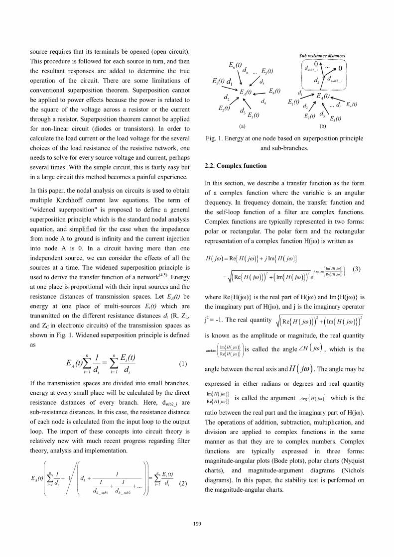
In this paper, the nodal analysis on circuits is used to obtain multiple Kirchhoff current law equations. The term of "widened superposition" is proposed to define a general superposition principle which is the standard nodal analysis equation, and simplified for the case when the impedance from node A to ground is infinity and the current injection into node A is 0. In a circuit having more than one independent source, we can consider the effects of all the sources at a time. The widened superposition principle is used to derive the transfer function of a network(4,5). Energy at one place is proportional with their input sources and the resistance distances of transmission spaces. Let EA(t) be energy at one place of multi-sources Ei(t) which are transmitted on the different resistance distances di (R, ZL, and ZC in electronic circuits) of the transmission spaces as shown in Fig. 1. Widened superposition principle is defined as

n ni

Ai=1 i=1i i

E (t)1E (t) =d d (1)

If the transmission spaces are divided into small branches, energy at every small place will be calculated by the direct resistance distances of every branch. Here, dsub2_i are sub-resistance distances. In this case, the resistance distance of each node is calculated from the input loop to the output loop. The import of these concepts into circuit theory is relatively new with much recent progress regarding filter theory, analysis and implementation.

_ 1 _ 2

1...

n ni

A ki=1 i=1i i

k sub k sub

E (t)1 1E (t) d =1 1d dd d

(2)

1d

2d

3d4d

5dnd …

1E (t)

2E (t)3E (t)

4E (t)

5E (t)nE (t)

AE (t) 1d

2d

3did

2 _sub id2 _1subd

…1E (t)

2E (t)3E (t)

nE (t)AE (t)

00

kd

Sub resistance distances

…

(a) (b)

Fig. 1. Energy at one node based on superposition principle and sub-branches.

2.2. Complex function

In this section, we describe a transfer function as the form of a complex function where the variable is an angular frequency. In frequency domain, the transfer function and the self-loop function of a filter are complex functions. Complex functions are typically represented in two forms: polar or rectangular. The polar form and the rectangular representation of a complex function H(jω) is written as

Imarctan2 2 Re

Re Im

Re ImH j

jH j

H j H j j H j

H j H j e

(3)

where Re{H(jω)} is the real part of H(jω) and Im{H(jω)} is the imaginary part of H(jω), and j is the imaginary operator

j2 = -1. The real quantity 2 2Re ImH j H j

is known as the amplitude or magnitude, the real quantity

Imarctan

ReH jH j

is called the angle H j , which is the

angle between the real axis and H j . The angle may be

expressed in either radians or degrees and real quantity

ImRe

H jH j

is called the argument Arg H j which is the

ratio between the real part and the imaginary part of H(jω). The operations of addition, subtraction, multiplication, and division are applied to complex functions in the same manner as that they are to complex numbers. Complex functions are typically expressed in three forms: magnitude-angular plots (Bode plots), polar charts (Nyquist charts), and magnitude-argument diagrams (Nichols diagrams). In this paper, the stability test is performed on the magnitude-angular charts.

199

2.3. Graph signal model for complex function

In this section, we describe the graph signal model of a typical complex function which is the same as the graph signal model of a feedback system. A negative-feedback amplifier is an electronic amplifier that subtracts a fraction of its output from its input, so that negative feedback opposes the original signal. The applied negative feedback can improve its performance (gain stability, linearity, frequency response, step response) and reduce sensitivity to parameter variations due to manufacturing or environment. Thanks to these advantages, many amplifiers and control systems use negative feedback. However, the denominator complex functions are also expressed in the graph signal model which is the same as the negative feedback system. A general denominator complex function is rewritten as

( ) ( )( )( ) 1 ( )

out

in

V s A sH sV s L s

(4)

This form is called the standard form of the denominator complex function. The output signal is calculated as

( )( ) ( ) ( )out in out

L sV s A s V s V sA s

(5)

Fig. 2 presents the graph signal model of a general denominator complex function. The feedback system is unstable if the closed-loop “gain” goes to infinity, and the circuit can amplify its own oscillation. The condition for oscillation is

2 1( ) 1 1 ;j kL s e k Z (6)

Through the self-loop function, a second-order denominator complex function can be found that is stable or not. The concepts of phase margin and gain margin are used to asset the characteristics of the loop function at unity gain. The conventional test of the loop gain, which is called “Barkhausen’s criteria”, is unity gain and -180o of phase in magnitude-phase plots (Bode plots)(6).

Fig. 2. Graph signal model of general complex function.

2.4. Alternating current conservation measurement

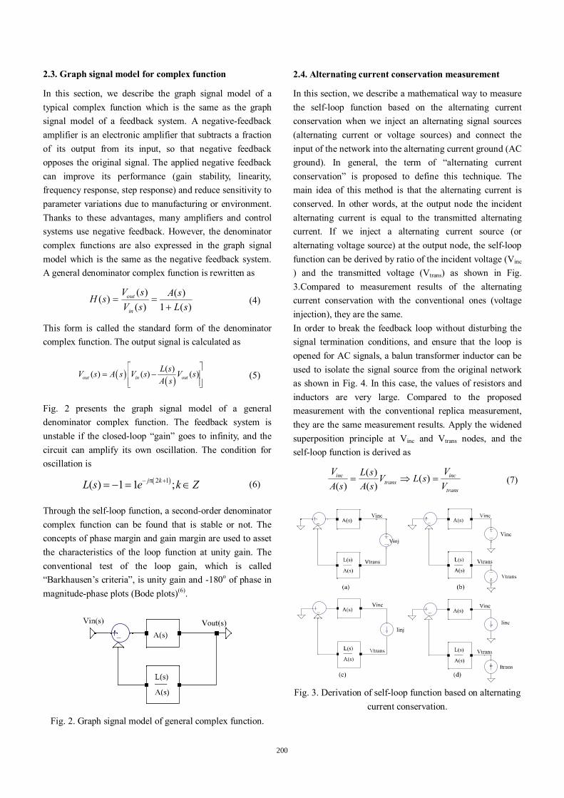
In this section, we describe a mathematical way to measure the self-loop function based on the alternating current conservation when we inject an alternating signal sources (alternating current or voltage sources) and connect the input of the network into the alternating current ground (AC ground). In general, the term of “alternating current conservation” is proposed to define this technique. The main idea of this method is that the alternating current is conserved. In other words, at the output node the incident alternating current is equal to the transmitted alternating current. If we inject a alternating current source (or alternating voltage source) at the output node, the self-loop function can be derived by ratio of the incident voltage (Vinc ) and the transmitted voltage (Vtrans) as shown in Fig. 3.Compared to measurement results of the alternating current conservation with the conventional ones (voltage injection), they are the same. In order to break the feedback loop without disturbing the signal termination conditions, and ensure that the loop is opened for AC signals, a balun transformer inductor can be used to isolate the signal source from the original network as shown in Fig. 4. In this case, the values of resistors and inductors are very large. Compared to the proposed measurement with the conventional replica measurement, they are the same measurement results. Apply the widened superposition principle at Vinc and Vtrans nodes, and the self-loop function is derived as

( ) ( )( ) ( )inc inc

transtrans

V VL s V L sA s A s V

(7)

Fig. 3. Derivation of self-loop function based on alternating

current conservation.

200

Fig. 4. Derivation of self-loop function based on balun transformer inductor injection method.

3. Analysis of first-order denominator complex function

3.1. First-order denominator complex function

In this section, we shall present the frequency response of a typical first-order denominator complex function. A general transfer function of the first-order denominator complex function is defined as in Eq. (8). Assume that all of the constant variables are not equal to zero. If the constant is smaller than zero, it is expressed as a complex number

( 20 ja a a j a e ). In this paper, the angular

of the constant is not written in details.

1( )H sas b

(8)

The simplified form of Eq. (8) is

arctan

2

1 1 1 1( )1 1

aj

bH s j eab b asb b

(9)

Here, the cut-off angular frequency is cutba

. The

magnitude of the complex function decreases very fast from the cut-off angular frequency. Therefore, the high-order harmonics of a step input are significantly reduced when it goes into the network.

3.2. Self-loop function of first-order denominator complex function

In this section, the characteristics of the self-loop function L(s) of the first-order denominator complex function are investigated. From Eq. (9), the self-loop function is defined as in Eq. (10). Through this function, it is easy to find that the first-order denominator complex function is stable, because the phase does not change when the angular frequency goes from 0 to infinity.

+-( )inV s

( )outV s

R

LZ sL

R

LZ sL injV

+ -iAV oAV

(a) (b)

Fig. 5. Models of RL LPF: (a) circuit, (b) measurement of self-loop function.

2( )ja aL j j e

b b

(10)

3.3. Analysis of RL low-pass filter

In this section, we shall present the frequency response of a first-order denominator complex function which is used in the ladder RLC low-pass filter. Figs. 5(a) and 5(b) show the model of circuit and the measurement of the self-loop function for an RL low-pass filter using alternating current conservation technique. Apply the superposition principle at Vout node, and we get

1 1 inout

L L

VV

Z R Z

(11)

Then, the transfer function and the self-loop function are defined as in Eq. (12). Due to analysis in Section 3.2, the self-loop function of the RL low-pass filter is a stable system, because the phase does not change when the angular frequency goes from 0 to infinity.

2

1 1( )11

( )

out

Lin

j

VH s

Z sLVRR

j L LL s j eR R

(12)

3.4. Stability test for RL low-pass filter

This section shows the stability test for the RL low-pass filter. The proposed model for this filter in Fig. 6(a) is designed at cut-off frequency f0 = 50kHz taking L =796 uH, and R=250 Ω. Fig. 6(b) shows the measurement of the self-loop function and Fig. 6(c) show the amplitude-phase plots of the transfer function and the self-loop function of the RL low-pass filter. At unity gain (50 Khz) of the self-loop function, the angular is 90 degrees. On the polar chart, real part of the self-loop function is equal to zero as shown in Fig 6(d). Compared to the simulation result with the mathematical analysis, they are the same.

201

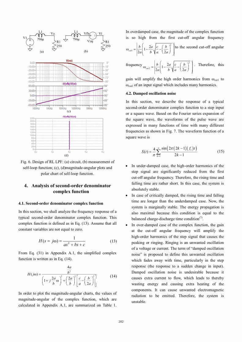
Fig. 6. Design of RL LPF: (a) circuit, (b) measurement of

self-loop function; (c), (d)magnitude-angular plots and polar chart of self-loop function.

4. Analysis of second-order denominator complex function

4.1. Second-order denominator complex function

In this section, we shall analyze the frequency response of a typical second-order denominator complex function. This complex function is defined as in Eq. (13). Assume that all constant variables are not equal to zero.

2

1( )H s jas bs c

(13)

From Eq. (31) in Appendix A.1, the simplified complex function is written as in Eq. (14).

2

2 2 2

4

( )2 21

2

abH j

a a c bjb b a a

(14)

In order to plot the magnitude-angular charts, the values of magnitude-angular of the complex function, which are calculated in Appendix A.1, are summarized on Table 1.

In overdamped case, the magnitude of the complex function is so high from the first cut-off angular frequency

2

121

2 2cutb a c ba b a a

to the second cut-off angular

frequency 2

221

2 2cutb a c ba b a a

. Therefore, this

gain will amplify the high order harmonics from ωcut1 to ωcut2 of an input signal which includes many harmonics.

4.2. Damped oscillation noise

In this section, we describe the response of a typical second-order denominator complex function to a step input or a square wave. Based on the Fourier series expansion of the square wave, the waveforms of the pulse wave are expressed in many functions of time with many different frequencies as shown in Fig. 7. The waveform function of a square wave is

1

1

sin 2 2 14( )2 1k

k f tS t

k

(15)

In under-damped case, the high-order harmonics of the step signal are significantly reduced from the first cut-off angular frequency. Therefore, the rising time and falling time are rather short. In this case, the system is absolutely stable.

In case of critically damped, the rising time and falling time are longer than the underdamped case. Now, the system is marginally stable. The energy propagation is also maximal because this condition is equal to the balanced charge-discharge time condition(7).

In over-damped case of the complex function, the gain at the cut-off angular frequency will amplify the high-order harmonics of the step signal that causes the peaking or ringing. Ringing is an unwanted oscillation of a voltage or current. The term of “damped oscillation noise” is proposed to define this unwanted oscillation which fades away with time, particularly in the step response (the response to a sudden change in input). Damped oscillation noise is undesirable because it causes extra current to flow, which leads to thereby wasting energy and causing extra heating of the components. It can cause unwanted electromagnetic radiation to be emitted. Therefore, the system is unstable.

202

f1 f3 f5 ft

A

0

0.5T

T

(b)

0

A

(a)

Fig. 7. Square wave: (a) waveform, spectrum, and (b) partial sums of Fourier series.

4.3. Self-loop function of second-order denominator complex function

In this section, we investigate the characteristics of the self-loop function L(s) on the magnitude-angular plots and the polar chart. The general transfer function and self-loop function are rewritten as in Eq. (16). The magnitude-angular values and the real-imagine values of the self-loop function, which are calculated in Appendix

A.2, are summarized in Table 2. In this work, the self-loop function is sketched on the magnitude-angular charts and polar plots.

2

2 2 22

2 2 2

4

( )2 2 21 2

2

4 2 2( )2

abH j

a a a c bj jb b b a a

a a a c bL j jb b b a a

(16)

4.4. Analysis of second-order RLC low-pass filter

In this section, we shall present the frequency response of a second-order RLC low-pass filter. Models of circuit and measurement of self-loop function for the second-order RLC low-pass filter are shown in Fig. 8. The transfer function and the self-loop function of this network, which are calculated in Appendix A.3., are simplified as

2

2

1 ; ( )1

LH s L s LCs sL RLCs sR

(17)

Table 1. Summary of magnitude-angular values of transfer function

Case Underdamped Critically damped Overdamped

Delta ( ) 2

2 4 02

c b b aca a

22 4 0

2c b b aca a

22 4 0

2c b b aca a

Module

( )H 2

22 2 2 2

4

4 2 212

ab

a a a c bb b b a a

2

22 2

4

4 21

ab

a ab b

2

22 2 2 2

4

4 2 212

ab

a a a c bb b b a a

Angular ( )H 2 2 2

4

arctan2 21

2

ab

a a c bb b a a

2

4

arctan21

abab

2 2 2

4

arctan2 21

2

ab

a a c bb b a a

2ba

2

1 4( )2

aHb

( )2

H

2

1 4( )2

aHb

( )2

H

2

1 4( )2

aHb

( )2

H

203

Table2. Summary of magnitude-angular values and real-imagine values of self-loop function

Case Underdamped critically damped Overdamped

Delta ( ) 2 4 0b ac 2 4 0b ac 2 4 0b ac

( )L j 2

2 2 2 24 2 22

a a c b ab b a a b

2 44 2a ab b

2

2 2 2 24 2 22

a a c b ab b a a b

( )L j 2 2 2

4

arctan2 2

2

ab

a c b ab a a b

2arctan

2ab

2 2 2

4

arctan2 2

2

ab

a c b ab a a b

5 22ba

( ) 1L ( ) 76.3oL ( ) 1L ( ) 76.3oL ( ) 1L ( ) 76.3oL

2ba

( ) 5L ( ) 63.4oL ( ) 5L ( ) 63.4oL ( ) 5L ( ) 63.4oL

ba

( ) 4 2L ( ) 45oL ( ) 4 2L ( ) 45oL ( ) 4 2L ( ) 45oL

Re ( )L j

2 2 22 22

a a c bb b a a

22ab

2 2 22 2

2a a c bb b a a

Im ( )L j

4ab

4ab

4ab

5 22ba

Re 2 5 Im 2 5 2 Re 2 5 Im 2 5 2 Re 2 5 Im 2 5 2

2ba

Re 1 Im 2 Re 1 Im 2 Re 1 Im 2

ba

Re 4 Im 4 Re 4 Im 4 Re 4 Im 4

(a)

(b)

+-( )inV s

( )outV s

1CZ

sC R

LZ sL

1CZ

sCR

LZ sL injV

+ -oAV iAV

Fig. 8. Model of circuit and measurement of self-loop

function for second-order RLC low-pass filter.

Then, the denominator is modified as:

2

22 2

4

1 12 1 22

R CLH s

RCs RCLC RC

(18)

The constraints of the stability are defined as

21 1 Instability2LC RC

(19)

21 1 Marginal stability2LC RC

(20)

21 1 Stability2LC RC

(21)

If R, L and C components are chosen based on the balanced

204

charge and discharge time condition |ZL|=|ZC|=2R at cut-off

angular frequency2

1 1=2LCLC RC RC

, this system is

called marginally stable(8).

4.5. Stability test for RLC low-pass filter

This section will present a stability test for an RLC low-pass filter. Three models of the second-order RLC low-pass filter are used to do the damped oscillation noise test. The marginally stable model is designed at cut-off frequency f0 = 50 kHz taking L =796 uH, C =3.18 nF, and R=250 Ω based on a balanced charge and discharge time condition as shown in Fig. 9(b). Figs. 9(a) and 9(c) are unconditionally stable (R=150), and unstable (R=500), respectively. Figs. 9(d), 9(e) and 9(f) are the measurements of the self-loop functions. Figure 10(a) represents the SPICE simulation results of the magnitude and phase of the RLC circuit on the frequency domain. In time domain, when the pulse signals go in to these models, the transient responses are shown in Figure 10(b).

Fig. 9. Models of circuits and measurements of self-loop functions for RLC LPF; (a),(d) unconditionally stable,

(b),(e) marginally stable, and (c),(f) unstable.

The damped oscillation noise (red) occurs in case of the unstable network. The overshoot of the unstable system can cause extra current to flow, thereby wasting energy and cause extra heating of the components. The measurements of the self-loop functions of the proposed models on the polar chart and the magnitude-angular plots are shown in Figs. 14(c),(d). In theoretical calculation at the cut-off frequency 50 kHz is 76.3 degrees.

Fig. 10. Frequency response (a), transient response (b) and (c), (d) polar chart and magnitude-phase plots of self-loop

function for second-order LPF; (brown) absolutely stable, (blue) marginally stable, (red) unstable.

205

Proceedings of the 8th IIAE International Conference on Industrial Application Engineering 2020

© 2020The Institute of Industrial Applications Engineers, Japan.

Our measurement results of self-loop functions show that

In stable case, phase is 98 degrees at 50 kHz,(phase margin = 82 degrees).

In marginally stable case, phase is 102.4 degrees at 50 kHz, (phase margin = 73.6 degrees).

In unstable case, phase margin is 116 degrees at 50kHz,(phase margin = 64 degrees).

On the polar plots of self-loop functions, the stability tests of these models are shown in Fig. 10(c). The characteristics of a self-loop function are divided into three regions: (brown) unconditionally stable, (blue) marginally stable, and (red) unstable. The simulation results and the values of theoretical calculation are unique. The constraints for passive components (R, L, C) are

Unconditionally stable (|ZL|=|ZC|>2R), phase margin is greater than 73.6 degrees at unity gain.

Marginally stable (|ZL|=|ZC|=2R), the phase margin is 73.6 degrees at unity gain.

Unstable (|ZL|=|ZC|<2R), the phase margin is smaller than 73.6 degrees at unity gain.

5. Design of ladder RLC low-pass filter

5.1. Analysis of ladder RLC low-pass filter

In this section, a ladder RLC low-pass filter is analyzed. This filter has been widely used because it is simple, versatile, and requires few components(9). The ladder RLC circuit and measurement of the self-loop function are shown in Figure 11. The ideal operational amplifiers are used and the effect of the Miller capacitor is neglected. The transfer function of this filter, which are calculated in Appendix A.4., is derived as

11

1 2 2 2 2

1( )1 1 1 11 1 L

C C C

H sR

Z RZ Z R Z R

(22)

From Eq. (22), the transfer function is rewritten as

2 2 2 21

1

2 2

1 1( )1 1 1 11

111 11

LC C

CL

C

H sZ

Z R Z RR

ZZ

Z R

(23)

From Eq. (23), we found that there are two stable conditions for this filter. Let us divide this transfer function into H1(s) and H2(s).

+- ( )inV s

( )outV sLZ sL1R

11

1CZ

sC

2R 22

1CZ

sC

AV

2U

1U

2R

11

1CZ

sCLZ sL

1R

3R1V

2V3V 4V 5V

+-( )inV s

2U

2R

1U

3R 4R1R

11

1CZ

sC

22

1CZ

sC

( )outV s

11

1CZ

sC 4R

(a)

(b)

(c)

Fig. 11. Models of ladder RLC LPF: (a) passive circuit, (b) active inductor using general impedance converter, (c)

design of active ladder RLC LPF.

The transfer function and the self-loop function of H1(s) are written as in Eq. (24). The characteristics of the self-loop function L1(s) are the same as in the analysis of the second-order RLC low-pass filter.

1 12 2

2 2

1 1 1( ) ; ( )1 11

LC

LC

H s L s ZZ R

ZZ R

(24)

The transfer function and the self-loop function of H2(s) are written as in Eq. (25).

2

2 21

1

2 2

2 22 1

1

2 2

1( )1 1

111 11

1 11( )

1 11

C

CL

C

C

CL

C

H s

Z RR

ZZ

Z R

Z RL s RZ

ZZ R

(25)

When the frequency compensation is considered, the transfer function of a ladder RLC low-pass filter is a third-order denominator complex function as in Eq. (26). It is very difficult to investigate the stable regions of this complex function. So, the measurement of the self-loop

206

function is very important to do the stability test for the ladder RLC low-pass filter. In this work, we firstly design the second-stage of the filter based the marginally stable condition. Therefore, the overall stability of the filter is also satisfied. The transfer function and the self-loop function of the ladder RLC low-pass filter are rewritten as

23 2

2 1 2 1 2 2

1 2 2 1 2 1 1 2

3 22 1 2 1 2 2

1 2 1 2 2 1 2 1

( )

1( )

RH ss R LC C s L C R C

s L R R C R R C R R

s R LC C s L C R CL s

R R s L R R C R R C

(26)

5.2. Analysis of general impedance converter

In this section, the passive inductor is replaced by a general impedance converter. The behavior of an inductor can be emulated by an active circuit(10). The general impedance converter is considered as a floating impedance as shown in Fig. 11(b).The feedback loops which are provided by the two op amps force V1 − V3 and V3 − V5 to zero.

1 3 5V V V (27)

Apply the superposition at node V3, and we get

2 43

2 2

1 1

C C

V VV

R Z R Z

(28)

The impedance of active inductor is designed as R1, R2, R3, and ZC are chosen properly. The value of this inductor is

3 2 32

1 1L out out

C

R R RRZ Z sCZR Z R

(29)

Here, Zout is the output impedance. This circuit converts a resistor to an inductor. Fig. 10 shows the model of the proposed design of the active ladder RLC low-pass filter.

5.3. SPICE simulations for ladder RLC LPF

In this section, SPICE simulations are carried out using the ideal operational amplifier with the gain bandwidth (GBW) = 10MHz and DC value of open loop gain (A(s)) = 100000. The ladder RLC circuit in Fig. 12(a) is designed for cut-off frequency f0 = 50 kHz taking C1 =127 nF, C2 = 31.8 nF, R1= 25Ω, R2 = 250 Ω, and L1 = 796uH. Fig. 12(b) represents the activeladder RLC circuit designed with C1 =127 nF, C2= 0.1 pF, C3=3.18 nF, R1= 25Ω, R2=R3= 1 kΩ, R4= 50 kΩ, and R5= 250 Ω.

Fig. 12. Proposed design of ladder low-pass filter; (a)

passive model, (b) active model, (c) frequency response: (brown) passive, (purple) active.

Fig. 12(c) represents the SPICE simulation results of the ladder RLC low-pass filter. The simulation results of the passive and the active ladder RLC low-pass filter are unique.

6. Discussion

The performance of a ladder RLC low-pass filter is determined by its loop self-loop function and step input responses. These measurements show how good a second-order low-pass filter is. The self-loop function of a low-pass filter is only important if it gives some useful information about relative stability or if it helps optimize the closed-loop performance. The self-loop function can be directly calculated based on the widened superposition principle. The alternating current conservation technique (voltage injection) can measure the self-loop function of low-pass filters. Compared to the research results with mathematical analysis, the properties of self-loop functions are the same. SPICE simulation results are included. Moreover, Nyquist theorem shows that the polar plot of self-loop function L(s) must not encircle the point (−1, 0) clockwise as s traverses a contour around the critical region clockwise in polar chart(11). However, Nyquist theorem is only used in theoretical analysis for feedback systems.

207

7. Conclusions

This paper describes the approach to do the stability test for a ladder RLC low-pass filter. The transfer function of this filter is a third-order denominator complex function. Moreover, the term of “self-loop function” is proposed to define L(s) in a general transfer function. In order to show an example of how to define the operating region of a multiple feedback filter, first and second-order denominator complex functions are analyzed. In overdamped case, the filter will amplify the high order harmonics from the first cut-off angular frequency ωcut1 to the second cut-off angular frequency ωcut2 of a step input. This causes the unwanted noise which is called ringing or overshoot.

The term of “damped oscillation noise” is proposed to define the ringing. The values of the passive components used in the filter circuit were chosen directly by the stable conditions. The passive inductor is replaced by a general impedance converter. All of the transfer functions were derived based on the widened superposition principle and self-loop functions were measured according to the alternating current conservation technique.

The obtained results were acquired to simulations using SPICE models of the devices, including the model of a two-stage operational amplifier. The frequency response from the proposed active ladder RLC low-pass filter is matched with the passive one.

In this paper not only the results of the mathematical model but also the results of simulation of the designed circuits are provided, including the stability test. The simulation results and the values of theoretical calculation of the self-loop function are unique. Furthermore, managing power consumption of circuits and systems is one of the most important challenges for the semiconductor industry(12,13). Therefore, the damped oscillation noise test can be used to evaluate the stability of a feedback system.

Acknowledgment

Foremost, we would like to express our sincere gratitude to advisor, Pro. Tanimoto (Kitami Institute. of Technology, Japan) for continuing supports.

References

(1) H. Kobayashi, M. Tran, K.Asami, A.Kuwana, H. San, "Complex Signal Processing in Analog, Mixed - Signal Circuits", Proceedings of International Conference on

Technology and Social Science, (Kiryu, Japan), May 2019.

(2) R. Schaumann and M. Valkenberg, Design of Analog Filters, Oxford University Press, 2001.

(3) M. Tran, N. Miki, Y. Sun, Y. Kobori, H. Kobayashi, "EMI Reduction and Output Ripple Improvement of Switching DC-DC Converters with Linear Swept Frequency Modulation", IEEE 14th International Conference on Solid-State and Integrated Circuit Technology, (Qingdao, China), Nov. 2018.

(4) M. Tran, N. Kushita, A. Kuwana, H. Kobayashi, "Flat Pass-Band Method with Two RC Band-Stop Filters for 4-Stage Passive RC Quadratic Filter in Low-IF Receiver Systems", IEEE 13th International Conference on ASIC (ASICON 2019) (Chongqing, China) Nov. 2019.

(5) M. Tran, Y. Sun, Y. Kobori, A. Kuwana, H. Kobayashi "Overshoot Cancelation Based on Balanced Charge-Discharge Time Condition for Buck Converter in Mobile Applications", IEEE 13th International Conference on ASIC (ASICON 2019) (Chongqing, China), Nov. 2019.

(6) M. Tran, Cuong Huynh, "A Design of RF Front-End for ZigBee Receiver using Low-IF architecture with Poly-phase Filter for Image Rejection", M.S. thesis, University of Technology Ho Chi Minh City – Vietnam, Dec. 2014.

(7) R. Middlebrook, "Measurement of Self-loop function in Feedback Systems", Int. J. Electronics, vol 38, No. 4, pp. 485-512, 1975.

(8) M. Tran, Y. Sun, N. Oiwa, Y. Kobori, A. Kuwana, H. Kobayashi, "Mathematical Analysis and Design of Parallel RLC Network in Step-down Switching Power Conversion System", Proceedings of International Conference on Technology and Social Science, (Kiryu, Japan) May 2019.

(9) B. Razavi, Design of Analog CMOS Integrated Circuits, 2nd Edition McGraw-Hill, 2016.

(10) H. Kobayashi, N. Kushita, M. Tran, K. Asami, H. San, A. Kuwana "Analog - Mixed-Signal - RF Circuits for Complex Signal Processing", IEEE 13th International Conference on ASIC (ASICON 2019) (Chongqing, China), Nov. 2019.

(11) J. Wang, G. Adhikari, N. Tsukiji, M. Hirano, H. Kobayashi, K. Kurihara, A. Nagahama, I. Noda, K. Yoshii, "Equivalence Between Nyquist and Routh-Hurwitz Stability Criteria for Operational Amplifier Design", IEEE International Symposium on

208

Intelligent Signal Processing and Communication Systems,(Xiamen, China), Nov. 2017.

(12) A. Sedra and K. Smith, Microelectronic Circuits, 6th ed. Oxford University Press, New York, 2010.

(13) M. Tran, "Damped Oscillation Noise Test for Feedback Circuit Based on Comparison Measurement Technique", 73rd System LSI Joint Seminar, Tokyo Institute of Technology, (Tokyo, Japan), Oct. 2019.

Appendix

A.1. Second-order denominator complex function

From Eq. (13), the transfer function is rewritten as

2 2 22

11( )

22 2 2

aH sas bs c b b c bs s

a a a a

(30)


2

2 2 2

4

( )2 21

2

abH s j

a a c bjb b a a

(31)

The magnitude-angular form of transfer function is

2 22 2 2 2

2 2 2

4 1( )4 2 21

2

4

( ) arctan2 21

2

aH jb

a a a c bb b b a a

abH j

a a c bb b a a

(32)

In critically damped case2

2c ba a

, the magnitude-angular

form of transfer function is

2 222 2

44 1( ) ; ( ) arctan

24 2 11

aa bH j H j

b aa abb b

(33)

At the cut-off angular frequency2cutba

, the

magnitude-angular form of transfer function is

22( ) ; ( ) arctan

2aH j H j

b (34)

A.2. Self-loop function of second-order denominator complex function

From Eq. (14), the self-loop function is rewritten as

2 2 24 2 2( )2

a a a c bL j j jb b b a a

(35)

The magnitude-angular form of self-loop function is

22 2 2 2

2 2 2

4 2 2( )2

4

( ) arctan2 2

2

a a c b aL jb b a a b

abL j

a c b ab a a b

(36)

The real-imagine form of self-loop function is

2 2 22 2 4Re ( ) ; Im ( )

2a c b a aL j L j

b a a b b

(37)

In critically damped case2

2c ba a

, the self-loop function is

2arctan22 44 4 2( ) 1

ja

ba a a aL j j j eb b b b

(38)

At the angular frequency ba


form of self-loop function is

( ) 4 2; ( ) arctan( 1) 45oL j L (39)


Re ( ) 4;Im ( ) 4L j L j (40)

At the angular frequency2cutba



( ) 5; ( ) arctan 2 63.4oL j L j (41)


Re ( ) 1; Im ( ) 2L j L j (42)

At unity gain of the self-loop function, we have

24( ) 1 1 1u u ua aLb b

(43)

Solving Eq. (43), the angular frequency u at unity gain is

5 22uba

(44)

209

The relationship between the angular frequency u and

the cut-off angular frequency 2cutba

is

5 25 2

uu cut cut

(45)

At unity gain angular frequency 5 22uba

, the

magnitude-angular form of self-loop function is

2( ) 1; ( ) arctan 76.355 2

oL j L j

(46)


Re ( ) 2 5; Im ( ) 2 5 2L j L j (47)

In underdamped case2

2c ba a


2 2 24 2 2( )2


(48)


22 2 2 2

2 2 2

4 2 2( )2

4

( ) arctan2 2

2


abL j

a c b ab a a b

(49)


2 2 22 2 4Re ( ) ; Im ( )

2a c b a aL j L j

b a a b b

(50)




2

2 22 2

2 2

2( ) 4 4 4 22

4( ) arctan arctan( 1) 452 4

2

o

a c bL jb a a

L ja c b

b a a

(51)




22 2

2 2

2( ) 4 1 52

2( ) arctan arctan 2 63.42 1

2

o

a c bL jb a a

L ja c b

b a a

(52)


2 22Re ( ) 4 4; Im ( ) 4

2a c bL j L j

b a a

(53)


, the


22 2

2 2

2( ) 2 5 2 2 5 12

2 5 2 2( ) arctan 76.355 22 5 2

2

o

a c bL jb a a

Arg L ja c b

b a a

(54)


2 22Re ( ) 2 5 2 52

Im ( ) 2 5 2

a c bL jb a a

L j

(55)

In overdamped case 2

2c ba a


2 2 24 2 2( )2


(56)


22 2 2 2

2 2 2

4 2 2( )2

4

( ) arctan2 2

2


abL j

a c b ab a a b

(57)


2 2 22 2 4Re ( ) ; Im ( )

2a c b a aL j L j

b a a b b

(58)




210

2

2 22 2

2 2

2( ) 4 4 4 22

4( ) arctan arctan( 1) 452 4

2

o

a c bL jb a a

L ja c b

b a a

(59)


2 22Re ( ) 4 4; Im ( ) 4

2a c bL j L j

b a a

(60)




22 2

2 2

2( ) 4 1 52

2( ) arctan arctan 2 63.42 1

2

o

a c bL jb a a

L ja c b

b a a

(61)


, the


22 2

2 2

2( ) 2 5 2 2 5 12

2 5 2 2( ) arctan arctan 76.355 22 5 2

2

o

a c bL jb a a

L ja c b

b a a

(62)


2 22Re ( ) 1 1; Im ( ) 2

2a c bL j L jb a a

(63)

A.3. RLC low-pass filter

+-( )inV s

( )outV s

1CZ

sC R

LZ sL

Figure 13. Circuit of RLC low-pass filter.

Apply the widened superposition at output node

1 1 1 inout

C L L

VV

R Z Z Z

(64)

Then, the transfer function is 1( )

1 11

out

inL

C

VH s

VZ

R Z

(65)


2 2

11

1 11

LCH s LLCs s s sR RC LC

(66)

Then, the denominator is modified as


A.4. Ladder RLC low-pass filter

+- ( )inV s

( )outV sLZ sL1R

11

1CZ

sC

2R 22

1CZ

sC

AV

Fig. 14. Passive Ladder RLC low-pass filter.

Apply the widened superposition at node VA, we get

1 1 1

2 2

( )1 1 11

1 1

inA

CL

C

V sV

R Z RZ

Z R

(69)

Do the same work at the output node, we get

2 2

1 1 1 Aout

L C L

VV

Z Z R Z

(70)

The transfer function of this filter is derived as

11

1 2 2 2 2

1( )1 1 1 11 1 L

C C C

H sR Z RZ Z R Z R

(71)

2 22

1

1 1 1 122 2 2

LCH ss s

RC RC LC RC

(67)

2

22 22

1 12

1 12 2 2 1 22

LC RCH s

RC s s RC RCLC RC

(68)

211

design of active inductor and stability test for ladder ... · magnitude-phase plots (bode...

Documents