design of an active acoustic sensor system for an...
TRANSCRIPT
Design of an Active Acoustic Sensor System for an Autonomous Underwater Vehicle
Minh Tu Nguyen Bachelor of Engineering Honours Thesis
1st November, 2004
Supervisor Associate Professor Thomas Bräunl
Mobile Robotics Lab Centre for Intelligent Information Processing Systems
School of Electrical, Electronic and Computer Engineering The University of Western Australia


i
Letter of Transmittal
Minh Tu Nguyen 4 Exeldia Place Belmont, WA 6104
1st November 2004
The Dean Faculty of Engineering, Computing and Mathematics University of Western Australia CRAWLEY WA 6009 Dear Professor Mark Bush, It is with great honour that I submit this thesis, entitled “Design of an Active Acoustic Sensor System for an Autonomous Underwater Vehicle” as partial fulfilment of the requirements of the degree of Bachelor of Engineering with Honours. Yours faithfully, Minh Tu Nguyen


iii
Abstract
Unstructured oceanic environments present great challenges to AUV navigation. However,
with continual improvements in sensor technology, new methods of navigating hazardous
underwater terrain are far more effective than ever before.
To date, much research has focused on maximising the functionality of AUVs at the expense
of cost. In contrast, this thesis aims to develop an active acoustic sensor system that
determines the distance an obstacle or landmark is from an AUV, while optimising cost
efficiency. Although this has been accomplished successfully on land-based autonomous
vehicles, these systems have not been implemented on AUVs. The focus is to design a system
that consists of four distance sensors directed to the port, starboard, bow and downward side
of the AUV.
The sensor system is custom-made using low cost components comprising the commercially
available Navman Depth 2100 transducer and the LM1812 ultrasonic transceiver chip. The
processing of sensor data will be accomplished by an Eyebot (Motorola 68332)
microcontroller.
Outcomes of the project included the successful design of a prototype sensor for the active
acoustic sensor system and successful testing and verification to demonstrate correct sensor
functioning, which provides the basis for further research in sensor development for the
University’s AUV, called the Mako. Final comments include a proposal for a control system
for the sensor application of wall-following, as well as recommendations for future
improvements and research.


v
Acknowledgements
Successfully completing this project would not have been possible without the tremendous
amount of time, assistance, and understanding of the people in my university life and my
personal life.
I would like to acknowledge my Honours supervisor, Associate Professor Thomas Bräunl,
whose guidance and expertise was pivotal to the project.
A very big thank you must also go to my family, especially my parents, for the infinite ways
in which they have supported my studies this year. A special thankyou must go to my sister,
brother-in-law and Terry O’Neill for all their proofreading. An extra special thank you to my
girlfriend, Clara Ng, to all my friends and fellow AUV team members, and to all the foreign
exchange students, for their support, humour and knowledge that kept me going through the
year.
Finally, thanks are also due to the members in the electronic workshop of the EE department,
especially Jonathon Brant and Ivan Neubronner, for their knowledge in hardware that was
crucial to the project.
vi
Table of Contents LETTER OF TRANSMITTAL............................................................................................................................ I ABSTRACT ........................................................................................................................................................ III ACKNOWLEDGEMENTS .................................................................................................................................V TABLE OF CONTENTS ................................................................................................................................... VI NOMENCLATURE ........................................................................................................................................... IX
ABBREVIATIONS ................................................................................................................................................ IX VARIABLES........................................................................................................................................................ IX
LIST OF FIGURES............................................................................................................................................ XI 1 INTRODUCTION........................................................................................................................................1
1.1 SENSOR SYSTEMS..................................................................................................................................1 1.2 PASSIVE AND ACTIVE SONAR SYSTEMS ................................................................................................2 1.3 ALGORITHMS FOR NAVIGATION WITH SONAR .......................................................................................2 1.4 PROJECT MOTIVATIONS.........................................................................................................................3 1.5 OUTLINE OF THE THESIS........................................................................................................................3
2 UNDERWATER SOUND TRANSMISSION AND NAVIGATION .......................................................5 2.1 PASSIVE DIRECTION OF ARRIVAL DETECTION.......................................................................................5
2.1.1 Time Delay Estimation.....................................................................................................................5 2.1.2 Direction of Arrival Calculations ....................................................................................................6
2.2 ACTIVE ACOUSTIC SENSOR SYSTEMS....................................................................................................7 2.3 FUNDAMENTALS OF SONAR SENSING ....................................................................................................8
2.3.1 Echo Sounding Principles................................................................................................................9 2.3.2 The Sonar Equation .........................................................................................................................9
2.4 TRANSMISSION LOSSES IN ACOUSTIC SYSTEMS ..................................................................................10 2.4.1 Transmission Intensity Losses of Acoustic Systems .......................................................................10 2.4.2 Scattering and Absorption Losses of Acoustic Systems .................................................................11 2.4.3 Frequency Dependent Losses in Acoustic Media...........................................................................12 2.4.4 Reverberation Considerations for Acoustic Systems .....................................................................13
2.5 CHARACTERISTICS OF ACOUSTIC TRANSDUCERS ................................................................................13 2.5.1 The Resonant Frequency of an Acoustic Transducer.....................................................................13 2.5.2 Directivity of Circular Transducers...............................................................................................14
2.6 THE EXTENDED KALMAN FILTER........................................................................................................16 2.6.1 The Development of Filter Equations ............................................................................................17 2.6.2 The Extended Kalman Filter Equations.........................................................................................19 2.6.3 Wall Following and the Extended Kalman Filter ..........................................................................19 2.6.4 Simultaneous Location and Mapping (SLAM)...............................................................................20
3 PROJECT REQUIREMENTS .................................................................................................................21 3.1 GENERAL REQUIREMENTS FOR AUTONOMY........................................................................................21
3.1.1 Competition Use ............................................................................................................................22 3.2 SOFTWARE REQUIREMENTS FOR SONAR NAVIGATION ........................................................................23 3.3 COST REQUIREMENTS FOR THE AUV ..................................................................................................23 3.4 THE COMPLETE REQUIREMENTS FOR THE SONAR SYSTEM..................................................................24
4 HARDWARE DESIGN .............................................................................................................................27 4.1 COMMERCIALLY AVAILABLE ECHO SOUNDERS ..................................................................................27
4.1.1 The Navman Depth2100 Echo Sounder .........................................................................................27 4.1.2 Shortcomings of the Navman Depth 2100 Echo Sounder ..............................................................28
4.2 NEED FOR A NEW DESIGN ...................................................................................................................29 4.2.1 Number of Transducers .................................................................................................................29 4.2.2 Choice of Transducer.....................................................................................................................30 4.2.3 Choosing a Design for a New Circuit ............................................................................................31 4.2.4 Design of a Circuit Prototype ........................................................................................................33

vii
4.2.5 Advantage of the Prototype Design ............................................................................................... 34 5 THE EYEBOT INTERFACE................................................................................................................... 35
5.1 CHOOSING THE INTERFACE ................................................................................................................. 35 5.1.1 Eyebot versus Onboard Transmission and Detection.................................................................... 35 5.1.2 Choosing a Direct Connection to the Eyebot ................................................................................ 36
5.2 SOUNDING FLOW CHART .................................................................................................................... 37 5.2.1 Mode of Operation......................................................................................................................... 37 5.2.2 Triggered Events and Subsequent Actions..................................................................................... 38 5.2.3 The Flow Chart.............................................................................................................................. 39
5.3 THE TIME PROCESSOR UNIT................................................................................................................ 41 5.3.1 The Input Transition Counter ........................................................................................................ 41 5.3.2 ITC Parameter RAM...................................................................................................................... 41 5.3.3 TPU Initialisation.......................................................................................................................... 43 5.3.4 Range and Resolution.................................................................................................................... 43
6 HARDWARE VERIFICATION AND EXPERIMENTAL RESULTS ................................................ 45 6.1 TESTING THE INTERFACE..................................................................................................................... 45
6.1.1 Testing the Eyebot Interface .......................................................................................................... 45 6.1.2 Testing the Echo Sounder Interface............................................................................................... 47 6.1.3 Testing the Combined Interface..................................................................................................... 49
6.2 DETERMINING THE CHARACTERISTICS OF ECHO SOUNDING ............................................................... 51 6.2.1 The Linearity of Returns ................................................................................................................ 52 6.2.2 Calibrating the Echo Sounder ....................................................................................................... 53 6.2.3 Mean Square Error for the Echo Sounder..................................................................................... 54 6.2.4 Minimum Detectable Static Distance ............................................................................................ 55 6.2.5 Maximum Detectable Static Distance............................................................................................ 56 6.2.6 Investigation of Signal Transmission Intensity .............................................................................. 57 6.2.7 Time Redundancies for a Simple Fault Tolerant System ............................................................... 61
6.3 PERFORMANCE OF THE SENSOR IN A DYNAMIC ENVIRONMENT .......................................................... 63 6.4 SUMMARY OF EXPERIMENTATION....................................................................................................... 67
7 NAVIGATION USING THE SONAR SENSORS .................................................................................. 69 7.1 ACTIVE SONAR APPLICATION ............................................................................................................. 69
7.1.1 The Wall Following Problem......................................................................................................... 69 7.1.2 Constraints of the System .............................................................................................................. 71
7.2 THE EXTENDED KALMAN FILTER........................................................................................................ 72 7.2.1 The Control Equations................................................................................................................... 73 7.2.2 Filter Predict and Correct Cycle ................................................................................................... 74
7.3 THE FEEDBACK CONTROLLER............................................................................................................. 75 8 FUTURE WORK....................................................................................................................................... 77
8.1 IMPROVING THE ECHO SOUNDER DESIGN ........................................................................................... 77 8.1.1 The Pulse Amplifier ....................................................................................................................... 78 8.1.2 The Time Variable Attenuator ....................................................................................................... 78
8.2 FUTURE RESEARCH ............................................................................................................................. 80 8.2.1 Designing a Passive Sonar Array.................................................................................................. 80 8.2.2 Testing the Control System ............................................................................................................ 80 8.2.3 Developing a Better Model for the Sensor System......................................................................... 81
9 CONCLUSION .......................................................................................................................................... 83 9.1 OUTCOMES OF THE PROJECT ............................................................................................................... 83
9.1.1 Designing the Echo Sounder Circuit ............................................................................................. 83 9.1.2 Interfacing to the Eyebot ............................................................................................................... 84 9.1.3 Hardware Verification and Experimental Results ......................................................................... 84 9.1.4 The Wall Following Algorithm ...................................................................................................... 85
9.2 FINAL WORD....................................................................................................................................... 85 APPENDIX A: THE TIME PROCESSOR UNIT............................................................................................ 87
A.1 CHANNEL CONTROL............................................................................................................................ 87 A.2 PARAMETER RAM .............................................................................................................................. 88
APPENDIX B: THE TIMER FREQUENCIES................................................................................................ 89

viii
APPENDIX C: PASSIVE SONAR APPLICATION........................................................................................91 C.1 TIME DELAY ESTIMATIONS .................................................................................................................91 C.2 DIRECTION OF ARRIVAL CALCULATION ..............................................................................................93
APPENDIX D: THE CONTENTS OF THE CD...............................................................................................95 D.1 THE THESIS .........................................................................................................................................95 D.2 THE PICTURES AND DRAWINGS...........................................................................................................95 D.3 THE CODE SET ....................................................................................................................................95 D.4 THE DATASHEETS AND RESEARCH..............................................................................................................95
REFERENCES ....................................................................................................................................................97

ix
Nomenclature
Abbreviations
Below is the list of abbreviations used in this thesis:
ADC – Analogue to Digital Converter AUV – Autonomous Underwater Vehicle AWGN – Additive White Gaussian Noise CPU – Central Processor Unit DOA – Direction of Arrival DSP – Digital Signal Processor EKF – Extended Kalman Filter FET – Field Effect Transistor GPS – Global Positioning System IRQ – Interrupt Request ITC – Input Transition Counter PAC – Pin Action Control RAM – Random Access Memory LC –Inductor-Capacitor LMS – Least mean square RF – Radio Frequency RMS – Root Mean Square ROBIOS – Robot Basic Input Output System SNR – Signal to noise ratio TBS – Time Base Select TDE – Time Delay Estimation TPU – Time Processor Unit
Variables
Below is the list of variables used in this thesis:
x – x coordinate of AUV xw – x coordinate of wall
y – y coordinate of AUV yw – y coordinate of the wall
θ – angle coordinate of AUV γ – angle of the wall
v – velocity of AUV(m/s) d – distance of AUV from wall(m)
ω – angular velocity (rads/s) r – distance of sensor from wall(m)
doffx – x distance from centre of AUV(m) doffy – y distance from centre of AUV(m)
α – thruster distance from centre of AUV(m) Ωmax – maximum thruster speed(m/s)
φ – half beamwidth of echo sounder X(k) – position state matrix of AUV
U(k) – input matrix for AUV control equations Ex(k) – process error
ξ(k) – measurement error of echo sounder F – the function matrix in the control equations
w – white Gaussian noise in process v – white Gaussian noise in measurement
z(k) – the distance measured by echo sounder H – the function matrix for z with respect to X

x
A(k) – Jacobian matrix of partial derivatives of F with
respect to X
W(k) – Jacobian matrix of partial derivatives of F with
respect to w
J(k) – Jacobian matrix of partial derivatives of H with
respect to X
V(k) – Jacobian matrix of partial derivatives of H with
respect to v
Q(k) – process error covariance matrix R(k) – measurement error covariance matrix
K – Kalman filter gain 2xσ - error covariance of the x coordinate
2yσ - error covariance of the y coordinate 2
θσ - error covariance of the angle coordinate
vdes – the desired velocity of the AUV ωdes – desired angular velocity of AUV µ – proportionality factor βi – ith experimental parameter ei – error in parameter i i - estimate of parameter i i~ - approximate value of parameter i

xi
List of Figures
Figure 2.1: Multipath environments cause ambiguity at the receivers.......................................7
Figure 2.2: Circular array demonstrating the discrete nature of data .........................................8
Figure 2.3: Echo sounder operation flow chart ..........................................................................9
Figure 2.4: The resonant and anti-resonant frequency of a transducer [14].............................14
Figure 2.5: Sound waves being received by a transducer.........................................................15
Figures 2.6 a), b), c) & d): Directivity for transducers of frequencies 5Hz, 40 kHz, 100 KHz
and 200 kHz, respectively ........................................................................................................16
Figure 3.1: Possible competition tasks including wall following, pipeline following, target
finding and obstacle mapping [18] ...........................................................................................23
Figure 4.1a) & b): the Navman echo sounder circuit board and transducer.............................28
Figures 4.2 a) & b): Receiver and transmitter sensitivities of a single transducer [19] ...........30
Figure 4.3: Design for an ultrasonic switch [21] ......................................................................32
Figure 4.4: Circuit layout of an ultrasonic switch ....................................................................32
Figure 4.5: Circuit diagram of the echo sounder circuit design [14]........................................33
Figure 4.6: Echo sounder communication lines with a microcontroller...................................33
Figure 4.7: Circuit board of prototype......................................................................................34
Figure 5.1: the 200µs pulse sent from the digital output of the Eyebot ...................................37
Figure 5.2: The flow chart for the echo sounding process .......................................................40
Figure 5.3: The ITC parameter RAM [22] ...............................................................................42
Figure 6.1: Experimental Setup for testing the Eyebot interface .............................................46
Figure 6.2: Two pulses separated by approximately 10ms ......................................................46
Figure 6.3: The experimental setup for the echo sounder interface .........................................47
Figure 6.4: No signal through the echo sounder.......................................................................48
Figure 6.5: 200µs pulse sent via the digital output, and the transducer is placed in water ......48
Figure 6.6: the pull down resistor placed between the logic output and the ground ................49
Figure 6.7: Signal when pull down resistor is used..................................................................49
Figure 6.8: The experimental setup for the combined interface...............................................49
Figure 6.9: Signal at the TPU channel when the transducer is not in the water.......................50
Figure 6.10: Signal that is received at the TPU channel when the transducer is in the water..51
Figure 6.11: Calculated time of flight over a range of distances for the echo sounder............52
Figure 6.12: Detection of an echo for different distances ........................................................57
Figure 6.13: Driver circuit to increase the voltage at the input of echo sounder......................58

xii
Figure 6.14: Oscilloscope display for when no driver is used ................................................. 58
Figure 6.15: Oscilloscope display for when driver is used...................................................... 59
Figure 6.16: Location of pin 6 and transformer windings on the circuit diagram [14] ........... 59
Figure 6.17: Frequency of LM1812 output.............................................................................. 60
Figure 6.18: Peak-peak voltage of transformer input .............................................................. 60
Figure 6.19: Peak-peak voltage of transformer output ............................................................ 60
Figure 6.20: Distance wooden rod is from sensor over time ................................................... 64
Figure 6.21 a) & b): Measuring distance from the rod over 500 time samples ....................... 64
Figure 6.22: 7th value select method on the tracking of a wooden rod .................................... 66
Figure 7.1: The wall following problem .................................................................................. 70
Figure 7.2: No returned echo at an angle greater than half the beamwidth ............................. 72
Figure 8.1: The pulse amplifier [14] ........................................................................................ 78
Figure 8.2: Time variable attenuator [14] ................................................................................ 79
Figure C.1: Signal impinging on the first sensor of passive array........................................... 92

1
1 Introduction
In the realm of automation and robotics, the surrounding environment is a challenge for any
autonomous vehicle to navigate due to the presence of stationary and moving obstacles. To
effectively negotiate the environment, a vehicle of this nature must be able to sense the
presence of obstacles and determine a path around them so as to avoid collision.
1.1 Sensor Systems
Just as there are many different types of robotics and autonomous vehicles, there are a variety
of different ways in which these vehicles can sense their surrounding environment. This is
particularly true of the underwater environment. Many surface autonomous vehicles use light
as a way of sensing. However, in the sub-sea environment, light becomes attenuated over
shorter distances meaning that vision becomes more difficult and RF communication and GPS
(global positioning system) become impossible. Therefore, an alternative means of sensing in
the water environment is required.
Although sound has limitations above water due to its short range, it travels very well in water
making it the medium of choice for underwater sensor systems. The use of sound for sensing
is commonly termed sonar, which is an acronym for SOund Navigation And Ranging. Sonar
is becoming increasingly more applicable to many fields including surveying, commercial
fishing and defence.
Sonar can be used in both an active and a passive mode. Active sonar requires a sonar
transducer to emit a signal which is then received after it has been reflected from a distant
surface. Passive sonar, however, only requires a receiver, called a hydrophone, to pick up
Design of an Active Acoustic Sensor System
2
signals emitted from a sound source. Active sonar allows the user to gather range information
as well as direction information, whereas passive sonar can only deliver direction information.
The development of a good sensory system is imperative for an autonomous underwater
vehicle to perform its required tasks efficiently. Although much of the research into sonar has
been conducted by defence and commercial groups, several universities have devoted
research towards creating more efficient sensory systems to improve AUV task completion.
1.2 Passive and Active Sonar Systems
Passive sonar has many applications especially in the military. It is used to identify and
monitor foreign vessels by tracking their characteristic sounds. In the commercial industry,
passive sonar is used to locate lost vessels that are submerged. Using an underwater acoustic
receiver, an acoustic beacon attached to the vessel can be detected and used to locate its
position.
Improving technology is, however, allowing submarines to become quieter and therefore
more difficult to detect with passive sonar. Thus, passive sonar is no longer adequate for all
underwater sensing scenarios. In addition, it is very difficult to range correctly with passive
sonar because it is only capable of giving the direction of arrival. The implication of this is
that two estimates of direction of arrival, from two distinct locations are required to
approximate the range of the sound source. In contrast, active sonar does not require a sound
to be emitted for an object to be detected and, the complete round trip time can be used to
calculate the range of the object. Due to the ‘beam-like’ nature of active sonar transducers,
they are also able to determine the direction of arrival of a signal.
1.3 Algorithms for Navigation with Sonar
Navigation underwater requires consideration of some key aspects. A mobile robot that
navigates in an unknown or changing environment needs to maintain a dynamic model of its
environment in order to update existing environmental knowledge. However, it is not possible
to create a dynamic map of the environment unless the AUV can detect objects that already
exist on an internal map, and any new objects that need to be added. Its sensors not only give
the AUV the ability to prevent collision of the AUV with any of the obstacles that lie within
an environment, but also give the AUV the ability to use the obstacles as landmarks from

Chapter 1 Introduction
3
which to navigate towards a target. A good sensor system is useless, though, unless an
appropriate adaptive algorithm for interpreting the sonar data is created.
1.4 Project Motivations
The completion of a sonar sensor system is of vital importance to the AUV because for an
AUV to become completely autonomous, it needs to be able to visualise the environment
around it.
Cost efficiency is an important goal of the project. The AUV may be used to research
commercially viable options for underwater robotics.
The project is, therefore, to develop a cost effective sonar system that can perform active
sonar. This means that a system must be developed that will not only work, but will also be
inexpensive to build.
1.5 Outline of the Thesis
In this paper, the problem of designing an acoustic sensor system for an AUV is addressed.
The paper is organised as follows.
Chapter 2 contains background information about underwater sound transmission and
navigation theory necessary to accomplish the design of a sensor system and a navigation
unit.
Chapter 3 outlines the requirements of general autonomy. This is incorporated with the cost
requirements for the system to provide a complete set of requirements for the sensor system.
Chapter 4 explains the shortcomings of commercially available echo sounders in achieving
the requirements outlined in chapter 3 and describes an improved prototype design for a new
echo sounder circuit.
Chapter 5 discusses the actual design of the interface between the prototype and the Eyebot,
including hardware decisions and software decisions that are needed to be made to achieve a
seamless interface.
Chapter 6 provides the verification and testing that is completed on the echo sounder circuit
and its interface with the Eyebot. Some key problems are identified and recommendations are
made regarding possible solutions.

Design of an Active Acoustic Sensor System
4
Chapter 7 discusses the development of navigational equations that will be the basis of
controlling the AUV using the acoustic sensor system. The extended Kalman filter (EKF) is
applied to the theoretical situation of wall-following and simultaneous location and mapping
(SLAM) with the AUV. The EKF is a set of equations, which provide an estimate of state
from the use of redundant sensor information. The SLAM uses the EKF to estimate its
position and the position of obstacles.
Chapter 8 discusses some potential future developments as well as further research areas.
Chapter 9 provides some concluding comments and a discussion of the project’s
achievements.
5
2 Underwater Sound Transmission and
Navigation
There are many aspects to the detection of sound underwater and the consequent navigation of
an AUV using sensors. What a sonar system attempts to do is determine the nature of the
environment using only sound so that the information can be used for navigational purposes.
Understanding the background in underwater sound transmission and navigation is crucial to
proceeding with any part of this project.
2.1 Passive Direction of Arrival Detection
After gaining an understanding of how different universities have developed their systems, it
is necessary to research further to determine how to better develop these ideas.
The Journals of the Acoustical Society of America proved to be a good source of information
on the field of signal processing and underwater acoustics. Amongst the literature, key articles
were found which addressed the subject of time delay estimation (TDE) and direction of
arrival (DOA) calculations.
2.1.1 Time Delay Estimation
Chern and Lin [1] came up with a simple and efficient method of TDE that involved a direct
computation combined with an adaptive least means squares TDE algorithm. This was
advantageous in accuracy and execution time; however it required that use of a continual
stream of data, which was computationally expensive. They also investigated the capability of
Design of an Active Acoustic Sensor System
6
TDE in a multipath environment. A multipath environment is one where the original signal
reflects off different surfaces before entering the receiver, resulting in delayed versions of the
signal at the receiver. This confuses the receiver as it does not know exactly which the true
signal is.
A completely different way of calculating the TDE, called the window-correlation technique,
was brought forward by Callison et al [2]. The method was built on the principles of the cross
correlation for TDE, which is briefly discussed briefly in [3]. They demonstrated that by
“windowing” the data record, events could be easily identified in a noisy environment. They
showed that this technique could be used for signals with a signal-to-noise ratio (SNR) of
down to 0 dB and this would prove very valuable in combination with low priced transducers.
2.1.2 Direction of Arrival Calculations
Once the TDE is calculated, the DOA can be calculated using the TDE’s. Berdugo et al [4]
investigated DOA calculations based on time delays. Their approach was different to the
usual maximum likelihood DOA estimators in that the DOA is extracted directly from the
delay times of the receivers and the geometry of the receivers. They also showed that the
azimuth and elevation estimator achieves the Cramer-Rao Lower Bound if the TDE achieves
the CRLB as well. This is one of the simplest methods of DOA calculations using the TDE’s.
Eigenstructure methods involve a projection of the signal onto a noise subspace, as a function
of direction, and finding a value that minimises this quantity. The value that minimises this
amount in the noise subspace will maximise the amount in signal subspace value, as the noise
and signal subspace are orthogonal. Cornell University used the MUSIC algorithm [5] to
calculate the DOA in 2002, which is an eigenstructure method. However, Paulraj and Kailath
[6] developed a similar method that could work on wave fronts with only partial spatial
coherence. The MUSIC algorithm assumes perfect spatial coherence.
This leads to the awareness that models are not perfect. Models that can better characterise
realistic systems in terms of relaxed assumptions and greater error will have a superior
performance in practice. Research needs to be completed in the area of errors in practical
situations. Daku, Salt and McIntyre [7] investigate locating the source in a multipath
environment.

Chapter 2 Underwater Sound Transmission and Navigation
7
Figure 2.1: Multipath environments cause ambiguity at the receivers
They investigate the effect that reverberations, or unwanted echoes, in the multipath
environment have on the ability of a system to locate a source. This is an important result as
the AUV will always be in these environments. They are able to obtain the variance of
localisation error and also demonstrate that in regions where the time delays of the multipath
signals matched the direct signal, large source localisation errors occur.
2.2 Active Acoustic Sensor Systems
Passive sonar does not allow an AUV to avoid obstacles. Therefore, in order to navigate
effectively around obstacles underwater, a well designed active sonar system needs to be
designed. This involves the proper design of a hardware system and a software system to
complement it. The hardware component must be designed to suit the nature of the navigation
that the AUV is supposed to complete. More complex navigation on larger AUVs require the
use of more sophisticated sonar systems than AUVs that only need to navigate simple
obstacle courses, but these come at a much greater cost. The software and navigation
algorithms work in unison with the hardware to allow for reliable navigation to be executed
by the AUV.
Many different approaches have been suggested as to how to implement a sensory system on
an AUV. A common approach is to create some form of imaging sonar. Williams et al. [8]
describe a system with ready-made imaging sonar that provides 360 degrees of sonar vision
for the AUV. This device can be directly linked to a navigational computer for analysis. The

Design of an Active Acoustic Sensor System
8
imaging sonar provides a full graphical display of the sonar returns that the device collects.
By using this data, the AUV has a continuous 360 degree view of its environment to allow it
to easily determine the locality of obstacles and itself within unstructured terrain.
In contrast, Ip and Rad [9] explore the use of discrete sonar sensors that are mounted at
specific intervals around the robot so that it can sense the proximity of obstacles that are
around it. This design is different from the one that is implemented by S. B. Williams et al.
(2000) in that the AUV does not have the full view of the surrounding environment, only
discrete distances at specific intervals around the robot as in Figure 2.2.
Figure 2.2: Circular array demonstrating the discrete nature of data
This design also has not been implemented on an AUV, but carries the same principle that
could be used with the AUV.
Yet another different approach is discussed by Ruiz et al [10]. The entire system for their
AUV consists of a Doppler velocity log, a tri-axial compass and side scan sonar. Side scan
sonar is similar to the 360 degree imaging sonar except that it can only see in a narrow field of
vision.
2.3 Fundamentals of Sonar Sensing
Sound transmission is a key part of underwater navigation as other forms of sensing, such as
light, do not have the range capabilities that sound has underwater. In order to successfully
use sonar to determine range of objects, one must understand how echo sounding works and
what may affect the detection of a sonar signal.

Chapter 2 Underwater Sound Transmission and Navigation
9
2.3.1 Echo Sounding Principles
The echo sounder works on a very simple principle. The operation of the transmitter and
receiver is similar to a basic AM transmitter and receiver.
A microcontroller, such as the Eyebot’s Motorola 68332 microcontroller, will send the sensor
a pulse signal. The sensor then uses this pulse signal to switch a carrier signal of particular
frequency on and off, similar to an AM transmitter switching between a maximum and zero
amplitude signal. This modulated pulse signal is then driven using a transformer to increase
the amplitude of the signal enough for the signal to travel a significant distance. The
transducer then converts the signal from electrical to acoustic vibrational energy through its
piezo-electric material. Figure 2.3 shows the operation of the echo sounder.
Figure 2.3: Echo sounder operation flow chart
On receiving the signal, the transducer converts the acoustic signal back to an electrical signal
and then the signal is amplified to increase the signal strength. It is then passed through a
frequency detector to determine if the right frequency has been received. On confirmation of
a correct signal, the logic output to the microcontroller is then driven low to indicate a
successful reception of the pulse signal.
2.3.2 The Sonar Equation
For active sonar where reverberations, or echoes, have a strong presence, the signal strength
needs to satisfy the following equation, in order for the acoustic system to be able to identify
the signal transmitted [11]:
(2.1)
• SL is the sound level of the transmitter, or intensity at the transmitter
DT DI- RLTSTL-SL ≥++2

Design of an Active Acoustic Sensor System
10
• TL is the loss of sound level during transmission of the signal in one direction.
• TS is the target strength and is dependent on the reflectivity of the given surface.
• RL is the level of reverberation, or echoes, encountered at the receiver.
• DI is the directivity index of the transducer, with a higher DI indicating more sound is
transmitted in the desired direction.
• DT is the detection threshold and is defined as the signal level required allowing
detection of the signal for 50 percent of the time.
All components are in decibels.
The equation is very similar for the passive sonar case, except the target strength is no longer
applicable because the signal is not reflected of a target surface, and the transmission loss is
only in one direction meaning that the multiplier for the TL is removed. The equation is as
follows:
(2.2)
2.4 Transmission Losses in Acoustic Systems
For sound to travel in a medium, the acoustic media must be compressible. A local
disturbance cannot instantaneously travel from one point to another, but must take a finite
amount of time to be transmitted, depending on the compressibility and the density of the
medium [12].
In most cases in any form of media, the intensity of sound waves continuously decreases over
the distance that they propagate. This can be usually accounted for by geometrical spreading
of a wave as well as the absorption and scattering of energy from the wave by the medium
involved. Then there are the frequency dependent components of loss and also reverberations
that may cause the degradation of the signal.
2.4.1 Transmission Intensity Losses of Acoustic Systems
The intensity at two radially different points in space would have the intensities 1I and 2I . For
spherical waves, the surface area is related to the square of the radius of the wave front, thus:
DT DI- RLTL-SL ≥+

Chapter 2 Underwater Sound Transmission and Navigation
11
(2.3)
However, usually the source provides some directionality for its sound waves and the
intensity rule cannot apply. More often, the equation is usually modified to:
(2.4)
The n in the equation is dependent on the directionality of the wave emitted from the source
and is non-integral and less than two.
2.4.2 Scattering and Absorption Losses of Acoustic Systems
Scattering and absorption of the medium provide another common loss of intensity of the
sound wave. The percentage loss over a particular distance is constant and can thus be written
as an exponential term with an absorption coefficient, a. This gives rise to the equation:
(2.5)
By taking the logarithms of both sides of the equation, and then rearranging the equation, the
propagation loss, N, or the difference of intensity can be termed as:
(2.6)
The H term accounts for the differences between the theoretical losses and that which are
observed, due to diffraction, reflection and refraction.
n
rrII ⎟⎟⎠
⎞⎜⎜⎝
⎛=
2
112
( )[ ]122
112 2exp rra
rrII
n
−⎟⎟⎠
⎞⎜⎜⎝
⎛=
( ) dBlog10 122
110 Hrr
rr
nN +−+⎟⎟⎠
⎞⎜⎜⎝
⎛= α
2
2
112 ⎟⎟
⎠
⎞⎜⎜⎝
⎛=
rrII

Design of an Active Acoustic Sensor System
12
2.4.3 Frequency Dependent Losses in Acoustic Media
Knowledge of the frequency dependent losses is important as it assists in determining what
frequency is ideal for echo sounding.
The losses are associated with dissipation of heat due to frictional forms of energy. There are
generally two losses of this form that are dominant in sound propagation; these are bulk
viscosity and absorption due to relaxation [13]. It is usually the bulk viscosity that has the
greatest effect on the attenuation of sound waves and is given by the following equation [2]:
(2.7)
In the equation, υ is the kinematic viscosity and ω is the angular frequency of the sound wave.
This loss has a square dependence on frequency.
The second loss of excess absorption due to relaxation can be explained by the absorption and
retransmission of energy from the medium. The time it takes for a particle to return to a
relaxed state after it has absorbed energy from a sound wave is called the relaxation time, τ. If
the energy is returned to the sound wave in phase, then the energy is added constructively.
However, if the energy is returned to the sound wave out of phase, then it causes destructive
interference. If the period of the wave is comparable to the relaxation time, then high
attenuation occurs. The equation for this phenomenon is given by [12]:
(2.8)
The αm term is the maximum attenuation coefficient at the relaxation frequency, 1/2πτ, and f
is the frequency of the sound wave.
It can be seen from the above losses, that the any acoustic system is limited in range. The
frequency of the sound wave propagating through a medium has a significant effect on the
attenuation of the sound wave in the medium and thus on the effective range of the
underwater acoustic system.
3
2
32
cvνωα =
22
2
2r
rm ff
ff+
= αα

Chapter 2 Underwater Sound Transmission and Navigation
13
2.4.4 Reverberation Considerations for Acoustic Systems
Acoustic signals, especially in an environment that is relatively enclosed, such as a swimming
pool, are backscattered off the many surfaces, meaning that the signal obtained by the receiver
will contain components from many different ray paths, masking the direct path signal. These
components are called reverberations. There is an upper limit to the source level that can be
transmitted. This is due to the fact that higher source levels represent higher reverberation
levels. This limit will be where the increase in signal to noise ratio (SNR) from the source
level will be non-beneficial for the receiver as it is countered by the decrease in SNR from
reverberation level, using equation 2.1. Thus the echo sounder must be designed to have just
enough signal level to transmit over a desired range. Any more signal level will contribute
unnecessarily to reverberation.
2.5 Characteristics of Acoustic Transducers
An acoustic transducer is a physical device that converts electrical energy to vibrational
energy and vibrational energy to electrical energy. This section discusses the characteristics of
an acoustic transducer. This includes the resonant frequency of an acoustic transducer and the
directivity of a transducer.
2.5.1 The Resonant Frequency of an Acoustic Transducer
All materials have a resonant frequency, including the membrane of an acoustic transducer.
This property of the material can be used to great advantage in the transmission and reception
of an underwater acoustic signal. Resonance is an increase in the oscillatory energy absorbed
by a material when the frequency of the oscillations matches the material's natural frequency
of vibration. This property is very useful because it means that by sending the right frequency
signal through the transducer, a higher percentage of power can be converted efficiently into
the transmission of the signal. The resonance of the transducer also has another valuable
property. Since the transducer can convert electrical signals to vibrational signals and vice
versa, the same effect can occur when the transducer is receiving a signal. This is
advantageous because the transducer material, therefore, naturally filters out noise from other
frequencies, resulting in a better signal to noise ratio when the signal is received. Transducer
materials can be made with the precise physical properties in order for it to resonate at a
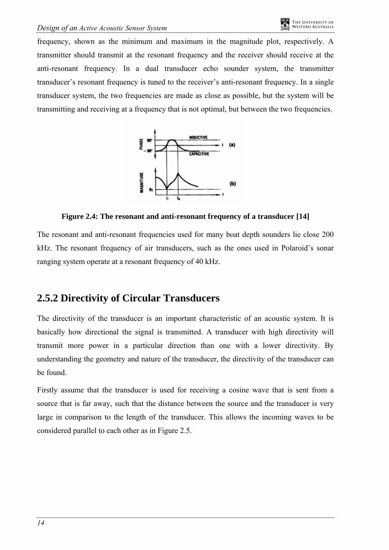
desired frequency. Figure 2.4 shows that a transducer has a resonant and anti-resonant
Design of an Active Acoustic Sensor System
14
frequency, shown as the minimum and maximum in the magnitude plot, respectively. A
transmitter should transmit at the resonant frequency and the receiver should receive at the
anti-resonant frequency. In a dual transducer echo sounder system, the transmitter
transducer’s resonant frequency is tuned to the receiver’s anti-resonant frequency. In a single
transducer system, the two frequencies are made as close as possible, but the system will be
transmitting and receiving at a frequency that is not optimal, but between the two frequencies.
Figure 2.4: The resonant and anti-resonant frequency of a transducer [14]
The resonant and anti-resonant frequencies used for many boat depth sounders lie close 200
kHz. The resonant frequency of air transducers, such as the ones used in Polaroid’s sonar
ranging system operate at a resonant frequency of 40 kHz.
2.5.2 Directivity of Circular Transducers
The directivity of the transducer is an important characteristic of an acoustic system. It is
basically how directional the signal is transmitted. A transducer with high directivity will
transmit more power in a particular direction than one with a lower directivity. By
understanding the geometry and nature of the transducer, the directivity of the transducer can
be found.
Firstly assume that the transducer is used for receiving a cosine wave that is sent from a
source that is far away, such that the distance between the source and the transducer is very
large in comparison to the length of the transducer. This allows the incoming waves to be
considered parallel to each other as in Figure 2.5.

Chapter 2 Underwater Sound Transmission and Navigation
15
Figure 2.5: Sound waves being received by a transducer
The wave that is received at the centre of the transducer is ( )tωcos . At a point that is r away
from the centre, the wave received is ( )krt −ωcos , where k is θλπ sin2 and λ is the wavelength
in the medium. The sensitivity is not uniform overall the surface, since the circular surface is
wider in the middle than on the sides.
This directivity function for a circular transducer is derived to be a first order Bessel function
of the first kind [12] as given below:
(2.9)
Polar plots from Matlab using equation 2.9 demonstrate the directivity of the transducer. As
can be seen by the plots in Figure 2.6, a higher frequency transducer produces a more directed
signal resulting in a greater range and finer angular resolution or that better reception of the
signal can be achieved. All the plots have the same maximum intensity of 1.
( )
2
221
Kl
KlJKD
⎟⎠⎞
⎜⎝⎛
=

Design of an Active Acoustic Sensor System
16
Figures 2.6 a), b), c) & d): Directivity for transducers of frequencies 5Hz, 40 kHz, 100 KHz and 200 kHz, respectively
Using the same principles in reverse, it is easy to see why the directivity function would be
the same for a transmitter of the same type of transducer.
Therefore, if a greater directivity for the transducer is required at the receiver, then a higher
frequency transducer will be necessary. However, this will come at a cost of more losses that
are presence with higher frequency signals, reducing the signal to noise ratio.
There is clearly an optimal choice for the frequency of the transducer, depending on the
application. For a better angular resolution, the frequency must be high. This results in greater
losses, and thus a smaller range. However, if the angular resolution is not important, then
choosing a lower frequency will result in a greater range for the sensor.
2.6 The Extended Kalman Filter
The Kalman filter is a set of mathematical equations that provides an efficient method to
estimate the state of a system that minimises the mean square error of the estimates. The

Chapter 2 Underwater Sound Transmission and Navigation
17
Kalman filter has been used to providing estimates of past, present and future states of a
system, meaning that the filter is a very powerful tool [15].
The Kalman filter is used to provide estimates of a state of a process or a system that is
governed by linear control equations. However, if a non-linear set of control equations are
used to define a system, another method of filtering is required.
The extended Kalman filter is set of equations that are used to solve non-linear control
equations. This works on a principle similar to that of a Taylor series, where the estimation is
linearised around the current estimate of the system, which may not have a linear relationship.
2.6.1 The Development of Filter Equations
Welch and Bishop [15] give an introduction to the Kalman filter. Control equations are
developed and then used to create the EKF equations.
The control equations for a non-linear system are as follows:
(2.10)
where the w and v terms are the random process and measurement noise variables, with zero
mean and a covariance of Q and V respectively. Now, using a process similar to a Taylor
series, the following equations have been developed to provide a consequent estimate based
on the current estimate of the state:
(2.11)
where ( )kX~ and ( )kz~ are approximate state measurements, ( )1ˆ −kX is the previous estimate
of the state.
The A, J, W and V matrices are therefore the Jacobian matrices of partial derivatives from
equation 2.10.
• A is the matrix of partial derivatives of function F with respect to X
• W is the matrix of partial derivatives of F with respect to w
• J is the matrix of partial derivatives of H with respect to X
• V is the matrix of partial derivatives of H with respect to v
( ) ( ) ( )( ) ( )( ) ( )( ) ( )kvkXHkz
kwkVkXFkX+=
−+−= 1,1
( ) ( ) ( ) ( )[ ] ( )( ) ( ) ( ) ( )[ ] ( )kVvkXkXJkzkz
kWwkXkXAkXkX
+−+≈
−+−−−+≈~~
11ˆ1~

Design of an Active Acoustic Sensor System
18
(2.12)
New errors can be given as:
(2.13)
where the two errors are:
kkz
kkx
zze
xxe
k
k
~~
~~
−=
−=
However, the equations in (2.13) appear very similar to the standard linear control equations
that an ordinary Kalman filter can estimate for. This leads to the use of the Kalman filter to
provide an estimate of the new error from (2.13), which will be called ke . Now according to
the ordinary Kalman filter equations:
(2.14)
Assuming that the predicted error is equal to zero, then equation 2.14 simplifies to:
(2.15)
Since ke representskxe~ , the following can be written:
(2.16)
However, since value of the position state cannot be known, it must be replaced with an estimate of the position state.
(2.17)
[ ][ ]
[ ]
[ ][ ]
[ ]
[ ][ ]
[ ]
[ ][ ]
[ ]j
iji
j
iji
j
iji
j
iji
vF
V
XH
J
wF
W
XF
A
∂∂
=
∂∂
=
∂∂
=
∂∂
=
,
,
,
,
( ) ( )[ ][ ] kxz
kx
kk
k
eJe
kXkXAe
η
ξ
+=
+−−−=~~
1ˆ1~
( )−− −+= kzkk eLeKeek
ˆ~ˆˆ
kzk eKe ~ˆ =
kkk
kkk
xk
exxxxe
eek
ˆ~~ˆ
~ˆ
+=−=
≡
( )kkkk
zk
kkk
zzKxx
eKxexx
k
~~ˆ
~~ˆ~ˆ
−+=
+=+=

Chapter 2 Underwater Sound Transmission and Navigation
19
2.6.2 The Extended Kalman Filter Equations
Deviating slightly from the equations given by Welch and Bishop [15], the W and the V
matrices are assumed to be identity matrices. This is done by assuming that the measurement
noise and process noise are both white and additive and applying this to equation 2.12. This
simplifies the filter equations.
The Kalman filter equations for the prediction stage are given as:
(2.18)
The filter equations for the correction stage, using equation 2.17 are:
(2.19)
To proceed with these equations, the first estimates from the prediction stage are set by the
user. The filter then corrects these estimates, using equation 2.19, before proceeding back to
the prediction stage and this process is continued recursively, back and forth through the
prediction and correction stages.
2.6.3 Wall Following and the Extended Kalman Filter
One common task for an autonomous vehicle is to follow the surface of a wall. This requires
the measurements of the compass and the speedometer of the vehicle to be very accurate.
However, with any measuring device, there will always be errors in their measurements,
which will affect the accuracy of any positioning that these devices estimate.
One way to decrease the errors in the estimations of positioning is to use other sensors to
more accurately assist with the localisation of the vehicle. The sonar sensors can be used to
assist with the correct positioning of the vehicle whilst measuring the distance from the edge
of the swimming pool. By fusing the sonar data with the speed and direction readings, a more
accurate position of the AUV can be found.
A Kalman filter allows for the fusion of sensor readings. However, for a control system for a
wall following task, the control equations are non-linear. This means that the ordinary Kalman
( ) ( ) ( )( )( ) ( ) ( ) ( ) ( )TT kQkAkPkAkP
kVkXFkX
11
,1ˆˆ
−+−=
−=−
−
( ) ( ) ( ) ( ) ( ) ( ) ( )[ ]( ) ( ) ( ) ( ) ( )( )[ ]( ) ( ) ( )( ) ( )−
−−
−−−
−=
−+=
+=
kPkJkKIkP
kXHkzkKkXkX
kRkJkPkJkJkPkK TT
ˆˆˆ
1

Design of an Active Acoustic Sensor System
20
filter cannot be used. Instead, a variation on the Kalman filter, known as an extended Kalman
filter, which attempts to develop a linear set of equations from the non-linear control
equations, is used.
2.6.4 Simultaneous Location and Mapping (SLAM)
Wallner and Dillmann [16] describe a method of map refinement that uses a local model of a
map stored in a database and readings from the sonar sensors to produce a model of the
robot’s perceivable environment. Their method of mapping the robot’s environment can be
broken down into two parts. The first part is the maintenance and refinement of the local map
that is stored within the robot’s memory. The second part is a grid based modelling of new
obstacles found by the robot and integrated into the current map.
The robot basically uses its sensor reading to discover obstacles. When it has located them, it
checks to determine if the obstacle is on the robot’s internal map. If it is not, then a new
obstacle is mapped. Otherwise, the new sensor reading is used to improve the robot’s idea of
where the obstacle is and increase the probability of the obstacle’s existence. This process of
increasing probability is continued until the object has presented enough information for it to
become ‘known’ to the robot. This, too, must use the EKF for more accurate localisation of
the obstacles and the robot.

21
3 Project Requirements
The main motivation for designing the AUV is to provide the basis for future research in
underwater control systems. Thus, the AUV needs to be designed so that it can be easily
adapted to suite many fields of research. However, the AUV must meet financial constraints,
so feasibility and functional analysis are significant elements in this project. The main goals
for the design of the AUV are therefore to create a system that is adaptable, functional and
cost effective.
3.1 General Requirements for Autonomy
A set of requirements needs to be developed for the AUV so that the AUV can be universally
autonomous. The meaning of universal autonomy is the control of a vessel, without external
communication, to navigate in any number of environments.
All that the AUV can use for navigational aids are its onboard camera and its complement of
sonar sensors. The camera is very limited in its ability to assist with navigation as it is pointed
downwards with no ability to pan left or right, up or down. The purpose of the camera is to
detect navigational markers or key objects on the pool floor that will assist the AUV in
orientating itself in the environment. Thus it is mainly up to the sonar system to determine the
proximity of and avoid collisions with obstacles and localise the AUV within the
environment. The sonar system will also assist with determining the depth of the AUV in the
pool.
The following basic requirements were derived for the sonar system to ensure the AUV’s
successful navigation of the environment using only sound:

Design of an Active Acoustic Sensor System
22
• To be able to avoid an obstacle that may hinder the path of the AUV
• To determine the range an obstacle is from the AUV
• To detect landmarks that may assist the orientation of the AUV
• To map new landmarks to assist in the localisation of the AUV
3.1.1 Competition Use
The best means of testing the AUV in different environments is to place the AUV into
competitions that have a changing set of tasks to accomplish each year. Not only does this
provide the AUV with a continually different environment to test its capabilities, but the
competitions allow respective AUV groups to have their systems judged against other groups.
This is important in the development of ideas as different groups become aware of new
approaches to solving problems associated with sensing and controlling an AUV.
As previously mentioned in chapter one, the AUVSI [17] annually hold competitions for all
types of autonomous vehicles including underwater vehicles. For the past few years, the
AUVSI has set similar tasks for the acoustic component of the competition mission. The goal
of these missions is to demonstrate vehicle autonomy by being able to sense acoustic cues in
the water and determine the direction of the cues.
A new competition will be introduced in the year 2005 that will enable university groups and
possibly industry groups in the Asia Pacific region to compete in an event with similar
aspirations to the underwater competition based in North America, but with different
competition missions and tasks. Possible tasks for a competition like this could include [18]:
• Wall following
• Pipeline following
• Target Finding
• Obstacle mapping

Chapter 3 Project Requirements
23
Figure 3.1: Possible competition tasks including wall following, pipeline following, target finding and obstacle mapping [18]
Though the AUV is not designed primarily for competition use, a competitive environment
will nurture the improvement of the design standards for the AUV.
3.2 Software Requirements for Sonar Navigation
Low level software needs to be written for the successful integration of sensors to the AUV
and to provide navigation control for the AUV.
Since most sensors relay a signal from their output, the AUV needs to be able to interpret
these signals and convert them to real data. This will often require low level programming of
the interface with the sensor.
Once this has been achieved, the sensor can be used to assist with the navigation of the AUV.
This will usually mean using some navigational algorithm to control the AUV to perform
certain tasks. The navigational control must be robust as the environment is never completely
predictable. The algorithms must be able to adapt to these environments.
3.3 Cost Requirements for the AUV
Financial constraints for the project are a limiting factor in the development of sonar system
for the AUV. Some requirements may need to be compromised or even removed so that more
important objectives can be completed.
Due to the limiting nature of these constraints, not all options for the design of a system are
feasible. Systems will need to able complete the tasks required of them at the cheapest
possible cost. Therefore, whilst some options may be able to perform better at completing a

Design of an Active Acoustic Sensor System
24
task, such as having a greater detection range, they may not be as feasible when compared
with a system that may perform slightly worse but is functionally adequate for what is
required and significantly decreases the cost of the system.
With this in mind, the design requirements of the sonar system need to be specified as the
minimal possible requirements that still allow the AUV to complete a set task at the least
expensive cost.
3.4 The Complete Requirements for the Sonar System
Incorporating the above requirements into the one set, the following are the requirements for
the sonar system of the AUV:
• Resolution for ranging of at least 5cm
• Maximum detection range of 5-10 metres
• Data rate of at least 10Hz
• Data must be easily transferred to the CPU or Eyebot
• System must be less than $1000
The requirements for range, resolution and data rate stem from the need for precision
navigation.
The data needs to be updated at a fast enough rate to enable the AUV to attain a more
continuous view of the environment. It becomes very difficult to steer the AUV when there
are relatively long intervals between the data. The data rate is the most important of the three.
If the data rate is insufficient, then the AUV may be blind at crucial times.
The range of the AUV is needed to enable the AUV to gain a larger view of the environment
around it. However, data rate is dependent on the range of the echo sounders. To have a
longer range, the signal must be stronger, so that the signal can travel further in the water.
However, this means that it will take longer for the signal to attenuate to a level that is
undetectable for the echo sounder when located in a highly reverberant environment. Only at
this level can the sensor begin to sound again. Thus, there is a trade off between the data rate
and the range of the echo sounder. The range of 5 metres has been chosen for the design of
this project.
It will not be possible to accurately gauge how far an object or surface is from the AUV
without a good resolution. This will be most obvious when the AUV is required to follow the

Chapter 3 Project Requirements
25
pool wall. A worse resolution will result in the AUV oscillating about a mean distance from
the wall. However, considering the size of the AUV and the pool environment in which the
AUV is in, a resolution of at most 5cm will suffice.
By having as many sensors as possible pointing in as many degrees as possible, the AUV is
better able to see all the obstacles around it and can therefore judge its position amongst the
obstacles better.
The achievement of these requirements for designing the sonar system of the AUV will fulfil
both objectives for the design of the AUV, which are functionality and cost effectiveness.


27
4 Hardware Design
The hardware design of the active sonar system is crucial to the AUV successfully
determining its distance from an obstacle. It is imperative the system be able to communicate
this information accurately to the CPU so that informed decisions can be made while the
AUV navigates the surrounding environment.
Although imaging sonar systems are preferable, due to financial constraint, a discrete sonar
system is employed. Consequently, the active sonar system is comprised of four individual
echo sounding units. Three facing the port, starboard, and bow sides for detection of lateral
obstacles and one facing down to provide depth measurement.
4.1 Commercially Available Echo Sounders
Although not of high quality, commercially available depth sounders are relatively
inexpensive, and are adequate for simple echo sounding tasks. It was necessary, however, to
determine the suitability of using depth sounders as proximity sensors on the AUV. One such
depth sounder was tested, and the results are described in the following sections.
4.1.1 The Navman Depth2100 Echo Sounder
Initially, the Navman echo sounder was purchased to provide depth readings for the AUV.
The idea came from the fact the boats could achieve depth readings from commercially
available echo sounders with reasonable accuracy at a far lesser cost than purchasing a digital
altimeter.
From this idea of depth measurements stemmed the idea that the echo sounder did not
necessarily only have to measure depth, but could also measure proximity of objects and

Design of an Active Acoustic Sensor System
28
surfaces in the lateral directions. Thus, although the echo sounders were initially only
intended for depth measurements, it was determined that an array of these sensors could
function as a complete acoustic sensor system.
However, an acoustic sensor system based on echo sounders requires a device of far superior
performance than the Navman Depth2100, which was consequently no longer suitable for the
project.
Figure 4.1a) & b): the Navman echo sounder circuit board and transducer
4.1.2 Shortcomings of the Navman Depth 2100 Echo Sounder
There are several key problems with the Navman echo sounder that make the device a poor
choice when it comes to use on the AUV. These problems are:
• An inaccurate resolution of 10cm
• A very slow data rate of 1 Hz
• A serial data line
• Lack of programmability
Having a resolution of 10cm means that the AUV will not be able to accurately maintain
specific distances from objects or maintain a specified depth. Since the echo sounder will be
used mainly for navigation and collision detection, the resolution needs to be better than 5cm,
as stated in chapter 3.
The data rate of 1 Hz is also very slow. This means that the AUV will not be able to adjust
quickly enough to any immediate changes to the environment, and must rely on the fact that
changes are gradual and the environment is predictable. However, the environment is never
completely predictable, thus the data rate of the echo sounder needs to be much faster to
accommodate for uncertainties within the environment.

Chapter 4 Hardware Design
29
The echo sounder is not programmable which means that the echo sounder parameters are not
controllable. The only aspect of the echo sounder that is controllable is turning the echo
sounder on or off. Thus, if data is required, the echo sounder is turned on, if the data is not
required, the sounder is turned off. This means that the sounder is not very practical for the
AUV.
The serial data line results in the following problems:
• Insufficient serial ports available on the Eyebot
• The need for development of a protocol to distinguish between each of the individual
echo sounders, which are operated simultaneously.
• Unacceptable delays in sound detection due to potentially longer than four second read
cycles.
Taking these factors into consideration, the Navman echo sounder is not functionally adequate
for use with the AUV. Furthermore, only by significantly changing the hardware, and
possibly the software, can the Navman echo sounder perform the tasks required.
4.2 Need for a New Design
A better option is to design a new echo sounder circuit board with the functionality required
to achieve the goals of the AUV. Since cost is such a limiting factor on the design of the
acoustic sensor system, there must be a significant amount of bias towards designing a
cheaper system. Also, as the AUV is completely operated on batteries, there must be a
consideration towards the power consumption of the system, but not at the expense of cost
benefits.
4.2.1 Number of Transducers
The number of transducers is an important decision concerning the design of an acoustic
system. The options are a one or two transducer echo sounder.
The main advantage of a two transducer system is that the resonant frequency of the
transmitter transducer can be matched to the anti-resonant frequency of the receiver, as
discussed in chapter 2. This will enable maximum power emission efficiency for the
transmitter and maximum power reception efficiency at the receiver. At other frequencies, the
transducer has some reactance, meaning power is not transferred as efficiently. A single

Design of an Active Acoustic Sensor System
30
transducer attempts to minimise the gap between the two frequencies, but as can be seen in
figure 4.2, they do not exactly match. The plots demonstrate the receiving anti-resonant
frequency as a peak in figure 4.2a), and the transmitting resonant frequency as a local
minimum in figure 4.2b). The optimal frequency for a single transducer will be close to both
the anti-resonant and resonant frequency.
Figures 4.2 a) & b): Receiver and transmitter sensitivities of a single transducer [19]
The problem is that the two transducer system is more expensive due to the need to purchase
two transducers. As there is a greater priority placed on cost than there is on power conversion
efficiency, the single transducer design is selected. The transducer will still resonate, but not
to the same extent as a two transducer system.
4.2.2 Choice of Transducer
There are many types of transducers available on the market, varying in both price and
quality. Obviously, the more expensive the transducer, the better the quality is. Thus, the
choice of transducer must hinge heavily on the type of application the transducer will be used
for. It must be investigated whether a less expensive transducer can fulfil the requirements for
the acoustic sonar system.
The type of application that the echo sounder is to be used for is basic echo sounding. This
application requires the use of a transducer that can effectively transmit and detect an acoustic
ping in water. Since the range for the echo sounder will be in the order of 10 metres, the
sensitivity of the transducer is not a very significant concern.
Another factor that is used to determine the type of transducer is the power consumption of
the transducer and the echo sounder as a whole, as stated earlier in this section. This can be
accomplished by choosing a transducer that outputs less power. However, the power
consumption is also closely linked to the range of the echo sounder. If low power

Chapter 4 Hardware Design
31
consumption is required, a smaller power acoustic ping can be transmitted, meaning that the
range of the echo sounder is reduced.
More expensive transducers only have slightly better physical characteristics than the much
cheaper transducers found on fish finders and boat depth sounders. The difference between
the two comes down to the fact that the more expensive transducer is developed closer to
specification than the cheaper transducer, and thus is more reliable and better specified.
However, for the purposes of the project, the cheaper Navman transducer is capable of
achieving the tasks at a lesser expense than the Reson TC 2111 and consumes less power
[19], [20]. Thus, since a greater weighting has been placed on producing the circuit at the least
cost, the choice of the inexpensive transducer over the more specified transducer has been
made.
4.2.3 Choosing a Design for a New Circuit
Much time was spent on investigating ways in which to approach the task of designing a new
echo sounder circuit that could fulfil the requirements set in Chapter 3. There is little
information on the design of underwater echo sounder circuits that is readily available both on
the Internet and in literature. The initial time spent researching methods focussed mainly on
adapting ultrasonic switches or AM transmitters. Figure 4.3 shows an example of an
ultrasonic switch that was tested for suitability [21]. Figure 4.4 shows the circuit layout on a
prototyping board.
The transmitter for this design was flawed, with respect to underwater echo sounding, as there
is less than 9V supplied to the transducer, with this voltage not being stepped up before
transmission. This meant that the system could only work within a range of less than 1m due
to a lack of signal intensity, which is not sufficient when the system is converted to an
underwater system.
The receiver was a very basic circuit of only a few parts. The first was a two transistor
amplifier. The second was an envelope detector consisting of a rectifier followed by a low
pass RC filter. The comparator at the end just sets the threshold for the logic. The simplicity
of this design meant that it was very limited in its ability to detect signals.
Other problems with these types of design are that they cannot be easily ported to a single
transducer system and that there are many components that will reduce the SNR of the

Design of an Active Acoustic Sensor System
32
system, decreasing the chances of detecting an echo. A circuit that caters for a single
transducer and has fewer components on the circuit board is needed for this project.
Figure 4.3: Design for an ultrasonic switch [21]
Figure 4.4: Circuit layout of an ultrasonic switch

Chapter 4 Hardware Design
33
4.2.4 Design of a Circuit Prototype
A design that utilised a National Semiconductor LM1812 ultrasonic transceiver chip was used
for development of the echo sounder circuit. Though the line of LM1812 chips is no longer in
production, they are still available from vendors internationally. This design was determined
to be the best to design a prototype with.
Figure 4.5: Circuit diagram of the echo sounder circuit design [14]
Obtaining a copy of the datasheet from National Semiconductors [14], it was found that the
chip could be used in a circuit (Figure 4.5), similar to one designed in the datasheet, which
could fulfil the task of underwater echo sounding.
Figure 4.6: Echo sounder communication lines with a microcontroller
Figure 4.6 demonstrates how the microcontroller communicates with the echo sounder circuit.
Basically, the circuit is a device that links to a microcontroller and only has provisions for
sending and receiving a 200 kHz frequency from the transducer. The pulse, which is
modulated to the 200 kHz carrier frequency, must be supplied by the microcontroller. Also,
any timing must be accomplished by the microcontroller.

Design of an Active Acoustic Sensor System
34
Figure 4.7: Circuit board of prototype
4.2.5 Advantage of the Prototype Design
It may seem like the whole system will be limited in ability due to the circuit’s simplicity, but
it is in fact quite beneficial. Since most of the echo processing is completed by the
microcontroller, the system becomes quite flexible, allowing it to closely match the design
requirements for the project.
Because the timing is handled by the microcontroller, the echo sounding system is no longer
limited by a set program, preset in a microcontroller of the echo sounder, like the Navman
echo sounder. In the Navman echo sounder, the echo sounding program, including the
transmission, reception and timing of the ultrasonic pulse was already preset in the echo
sounder’s microcontroller. The problem with this was that it is virtually impossible to
reprogram the microcontroller with more efficient code, as the code set for the
microcontroller is unknown. Thus the only output possible from this echo sounder is the serial
data in the NMEA 0183 protocol format, which only provides serial data at a rate of 1Hz.
Thus the key parameters of range, resolution and data rate can be adjusted on the new circuit
prototype.
Since the input and output of the echo sounder are only logic and not in serial form, they can
be easily interfaced to any microcontroller’s digital output and input (IO) with no need to
provide a protocol for transferring data. Also, with the basic input and output of the circuit, it
is not difficult to interface more than one device to the digital IO, as microcontrollers usually
have an abundance of IO ports. Thus, interfacing with the Eyebot is much simpler.

35
5 The Eyebot Interface
The interfacing of the echo sounder to the Eyebot is an important design step because without
proper interfacing, both in hardware and software, the sensor will not be able to communicate
information to the Eyebot, rendering the sensor useless. Design choices such as the type of
interface, method of connection and implementation of software are discussed in this chapter.
5.1 Choosing the Interface
The echo sounder circuit is very basic in its technique for transmitting and receiving a signal.
The circuit provides a modulated signal that needs to be switched on and off for an acoustic
pulse to be transmitted. The return signal is then detected by the circuit and represented by a
low on the circuit’s logic output. There is no provision for the processing of distance
measurements by the echo sounder. All this must be completed on a different circuit or
microcontroller. Before the echo sounding circuit prototype can be used with the Eyebot, an
interface with the Eyebot needs to be established.
5.1.1 Eyebot versus Onboard Transmission and Detection
There are two ways to establish a connection between the echo sounder and the Eyebot, each
with there own benefits and disadvantages, which need to be assessed so that the most
effective solution can be found.
The method of performing the signal processing on the Eyebot’s Motorola 68332
microcontroller is preferred, as opposed to performing it on a separate microcontroller. The
reasons for this are:

Design of an Active Acoustic Sensor System
36
• There is no need to set up a transfer protocol between the Eyebot’s microcontroller
and the other microcontrollers. If the data was processed separate from the Eyebot
microcontroller, then the data would need to be transferred to the Eyebot. The only
solution is to send data via a serial protocol. This would consume much time, and it
would be difficult to multiplex multiple sounders to the one Eyebot. It is more
efficient to process the data on the Eyebot.
• There is no need to purchase other microcontrollers and learn the code set for them.
• The Motorola chip has a theoretical resolution capability of up to 238.4ns which is
more than sufficient for echo sounding.
The only disadvantage of this solution is that the Eyebot will not be able to process other data
during the detection and processing of the data from the echo sounder, which may have an
effect on the timing of other processes. However, as long as this is taken into consideration
whilst designing the interface, then the problem can be minimised or even eliminated.
Thus the choice is clear that the Motorola MC68332 CPU (Central Processing Unit) on the
Eyebot will be used for the signal detection of the echo sounder. The Motorola
microcontroller has a number of features allowing for flexibility in the development of an
interface between the Eyebot and the echo sounder.
5.1.2 Choosing a Direct Connection to the Eyebot
The problem lies in how to utilise the functions available on the CPU to effectively create an
interface. The solution to the problem requires choosing the most effective method of
providing the input to the echo sounder and of receiving the output returned from the echo
sounder.
The echo sounder has two pins, which connect to a microcontroller. One pin is the key input
where the CPU sends the required pulse signal that will be modulated with the 200 kHz
carrier frequency and transmitted through the transducer. The second pin that connects to the
CPU is the logic output of the echo sounder. This output will be pulled low only when there is
a 200 kHz signal received on the transducer line. This may occur several times for every pulse
that is transmitted because the echoes from different surfaces will be just delayed versions of
the signal. Therefore, the Eyebot interface is basically a pulse signal through the key input
pin, followed by the delayed reception of a number of pulse echoes.

Chapter 5 The Eyebot Interface
37
The digital output of the Eyebot is adequate to transmit the sonar pulse as the CPU can be told
to switch on the digital IO, then wait for precisely the right amount of time and then finally
switch the digital output off. This is seen in Figure 5.1.
Figure 5.1: the 200µs pulse sent from the digital output of the Eyebot
The best way to accomplish the detection of a signal on the logic output of the echo sounder is
to provide some way for the echo sounder to interrupt the CPU when the logic output goes
low. This ensures that the exact times are recorded for processing. The interrupt system of the
CPU allows an external device or one of the microcontroller’s modules to interrupt the
processor execution. The best approach to interrupting the CPU by the echo sounder is
through programming one of the microcontroller’s modules. Since the recording of the
transmission and reception times requires a timer, using the Time Processor Unit (TPU) is the
optimal way to interface the logic output of the echo sounder.
5.2 Sounding Flow Chart
To establish exactly how the echo sounder unit will function with the Eyebot, a complete echo
sounding flow chart needs to be created and the functions required for the echo sounding
process need to be identified.
5.2.1 Mode of Operation
The first step before creating the flow chart is to determine when the echo sounder will be on.
The options for data collection are to have the echo sounder continuously collecting the data
and returning it to the Eyebot, or to only collect the data when the Eyebot requires it.
The latter approach is chosen over the former for two main reasons:

Design of an Active Acoustic Sensor System
38
• The sounding process is not time triggered but event triggered, removing the need to
implement an interrupt for this process. If a problem arises with the use of CPU timed
interrupts, it may cause timing errors in the rest of the timed events on the CPU
interrupt vector table. It is wiser to implement the commencement of sounding as an
event triggered process.
• The data is guaranteed to be current. If the echo sounder were to continually record
data, there would be a period of time when the data does not refresh in the cycle. If
the Eyebot were to read the data at the end of this time, then the data would no longer
be current. The better approach is to commence sounding when data is required,
ensuring the data is up to date.
5.2.2 Triggered Events and Subsequent Actions
The flow diagram has to be carefully designed to remove all time interrupts that may be
necessary, such as the reading of the data and the timing out of the echo sounder when no
pulse is returned. These may cause timing errors if used incorrectly.
The two timed events in the echo sounder’s operations are:
• Reading of the data variables
• Time out of the TPU channels if there is no returned signal
These events require the use of timers to ensure the correct timing of these events. However,
it is desirable to remove the use of interrupts for these events.
Instead of using a time interrupt, a wait is used to determine when to read the data, since the
wait time will be very small. For a 5m range, the time of flight is 6.69ms in fresh water. The
end of the wait time marks the time out of the echo sounder if the pulse is not received,
meaning that an interrupt is not required for this task either.
If the channels time out, the CPU turns the channels off, raises the new data flag and moves
the maximum value for distance into the distance variable of the C program. This indicates
that no return pulse was registered for the echo sounding cycle and thus the distance is
assumed beyond the range of the sonar.
The reading of data requires only the returning of the distance variable in the C program.
The reception of the echoes must rely on the TPU capabilities to accomplish the interrupt
which means that new code must be created for these operations using assembly language.

Chapter 5 The Eyebot Interface
39
Care must be taken to ensure that the interrupt requires little time to process to make sure
there are minimal timing problems.
When the CPU is interrupted by the reception of the returned signal, the CPU immediately
turns the channel off, and then checks the new data flag. If it is low, it raises the flag and then
stores the data from the channels’ registers. If it is high, then the interrupt does not do
anything. This is because the channel has timed out.
The echo sounding process is not time triggered but event triggered for reasons stated earlier
in section 5.2.1.
On the triggering of the transmission stage, the CPU must clear the new data flag and
commence the operation of all TPU channels involved with echo sounding. Following this,
one of the digital output pins of the Eyebot is switched on, and then the switched off after a
200µs wait.
The reason for switching the channel on before the pulse is transmitted is because the TPU
channels have the capability to record the transition time of two events. By commencing the
channels before the pulse, the TPU channels can record the time of the transmitted pulse as
well as record the time of the received pulse. Thus the TPU channels carry the two times
needed for distance calculations in its registers, meaning that the CPU does not need to obtain
the transmit time by other means.
The CPU must then wait 10ms for the possible interrupt, triggered by the reception of the
echo, to occur. As explained earlier in this section, if the interrupt does not occur, then the
channel times out.
5.2.3 The Flow Chart
Figure 5.2 is a diagram for the operation of the echo sounder. The 10ms wait will be sufficient
time for the received pulse to trigger an interrupt on the TPU channel or for the TPU channel
to time out, as long as the reflector is within the 5-10m maximum range that is require of the
sensor.
It is assumed that the echoes will attenuate much quicker than the rate at which data is
required from the Eyebot. Though this will be the case for most instances, it may be possible
to create an error by calling a new echo sounding process before the reverberations, or
secondary echoes, have time to dissipate, especially when more power is used. This must be
taken into account when programming the control system that uses the echo sounder.

Design of an Active Acoustic Sensor System
40
By observing the flow chart, it can be seen that four C functions need to be written for the
cycle of the echo sounder; one for the transmission of the acoustic pulse, one for the reception
interrupt, one for the timing out of a TPU channel and one for the reading of the data. This
requires setting the low level parameters of the TPU.
Figure 5.2: The flow chart for the echo sounding process

Chapter 5 The Eyebot Interface
41
5.3 The Time Processor Unit
The TPU module is a very powerful and very flexible module of the Motorola
microcontroller. The main advantage of the TPU module is that its timing is completely
independent of the CPU instruction timing once it has been initialised [22].
The TPU module solves the problem of multiple interrupts to the CPU because the TPU can
be used to count the number of pulses and only interrupt the CPU when the correct number of
pulses has been registered. The TPU channel also solves the problem of interfacing multiple
echo sounders to the Eyebot. Since the entire signal processing is accomplished with the CPU,
the echo sounder need only send the return pulses in the form of logic outputs. These can be
directly connected to the TPU channels and, since there are up to 16 available channels, there
is no difficulty interfacing a small number of echo sounders to the same CPU.
5.3.1 The Input Transition Counter
With the TPU channels, there are specific functions that will allow for the detection of pulses.
The best option for the reception of the echo sounder’s logic output is the Input Transition
Counter (ITC) function of the TPU channels. The ITC mode allows a specific number of input
transitions to be registered.
5.3.2 ITC Parameter RAM
For the correct operation of the ITC function, the parameter RAM of each channel must be
set. The channels’ parameter RAM stores all the information about the operation of the
channel at any one time and also contains the data registers that can store data from a
particular operation, such as times or number of transitions.
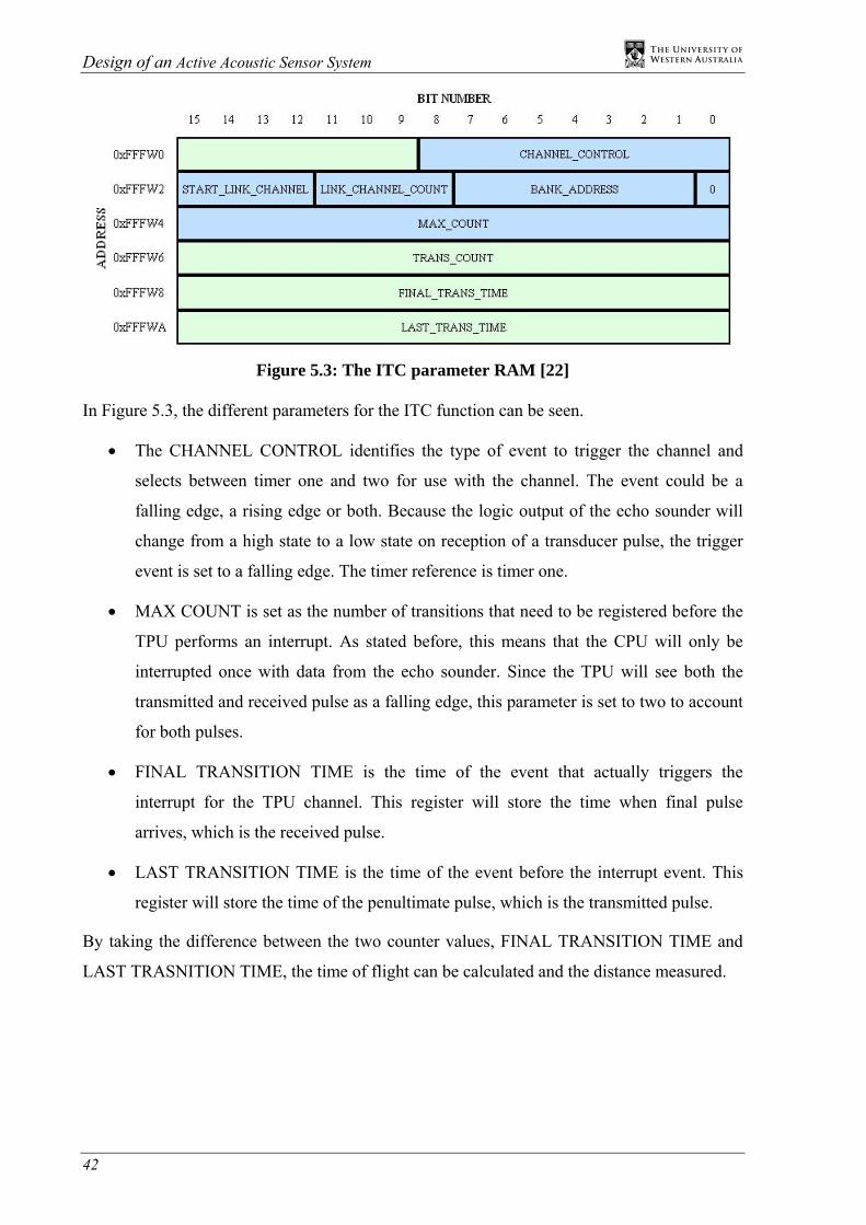
Design of an Active Acoustic Sensor System
42
Figure 5.3: The ITC parameter RAM [22]
In Figure 5.3, the different parameters for the ITC function can be seen.
• The CHANNEL CONTROL identifies the type of event to trigger the channel and
selects between timer one and two for use with the channel. The event could be a
falling edge, a rising edge or both. Because the logic output of the echo sounder will
change from a high state to a low state on reception of a transducer pulse, the trigger
event is set to a falling edge. The timer reference is timer one.
• MAX COUNT is set as the number of transitions that need to be registered before the
TPU performs an interrupt. As stated before, this means that the CPU will only be
interrupted once with data from the echo sounder. Since the TPU will see both the
transmitted and received pulse as a falling edge, this parameter is set to two to account
for both pulses.
• FINAL TRANSITION TIME is the time of the event that actually triggers the
interrupt for the TPU channel. This register will store the time when final pulse
arrives, which is the received pulse.
• LAST TRANSITION TIME is the time of the event before the interrupt event. This
register will store the time of the penultimate pulse, which is the transmitted pulse.
By taking the difference between the two counter values, FINAL TRANSITION TIME and
LAST TRASNITION TIME, the time of flight can be calculated and the distance measured.

Chapter 5 The Eyebot Interface
43
5.3.3 TPU Initialisation
To initialise the TPU and its channels, a number of other registers need to be set in assembly
language. A full listing of the parameters that need to be set, as well as how they should be
set, is given in Appendix A.
This initialisation must be run in order for the TPU and its channels to function correctly. This
includes setting the parameter RAM of the TPU channels.
5.3.4 Range and Resolution
The range and resolution of the echo sounder are important parameters that can be
determined by the TPU. There is a trade-off between these parameters because the counters
on the TPU are 16 bit, which increment on every TPU clock pulse. This means that when the
counter reaches a value of 65535, it resets to 0 and then continues counting. What this means
is that there is a maximum range of 65535 counts before there is ambiguity in the counter
value. For example, a count of 1 would be the same as 65537 according to the TPU. The clock
pulses to the counters can be set to different frequencies meaning that the effective range can
be increased, but this comes at the expense of the resolution. By having a lower frequency, the
range would increase because each clock pulse is longer, but the resolution is worse as it can
only resolve times in lengths of the clock pulse.
Herein lies the problem, which is to achieve the best possible resolution whilst still achieving
a good range. A good range for the echo sounder in a pool environment is 5m. The AUV only
needs to know what is immediately in its proximity. To convert the distance range into a time
range, the following equation is used, as well as the speed of sound in water of 1481m/s [23].
(5.1)
Thus, the effective range of the echo sounder needs to be approximately 6.75ms. Comparing
these amongst the values in Appendix B, it is observed that the resolution possible is actually
the best possible resolution, which is 238.4ns. This equates to a theoretical distance resolution
ms75.6range time1481
52sound of speed
range distance2range time
=
×=
×=

Design of an Active Acoustic Sensor System
44
of approximately 17.8µm, which is more than sufficient for the purposes of echo sounding.
Thus, for the project, a time resolution of 238.4ns and a range of 15.6ms are chosen.

45
6 Hardware Verification and
Experimental Results
The echo sounder needs to be properly tested and verified before it is implemented as a sensor
system for the AUV. The interface must work, so that the echo sounder can communicate
information to the Eyebot. The characteristics of the echo sounder need to be tested to
uncover any flaws in the system and to ensure an accurate model of the sensor system.
6.1 Testing the Interface
It is vital to individually test both the interface to the Eyebot and the interface to the echo
sounder so as to avoid any mismatch in voltage between the two components. A voltage
mismatch could potentially cause serious circuitry damage. In addition, diagnosing errors in
either component is more difficult once the two units are connected.
6.1.1 Testing the Eyebot Interface
Before connecting the echo sounder, the TPU channels on the Eyebot are tested to ensure that
they are functioning correctly. To proceed with the testing, a simple experiment is set up. A
connection from a digital output pin to one of the TPU channels is made using a 1kΩ resistor.
Figure 6.1 is a picture of how the experiment was set up. The resistor is to ensure that if there
is a voltage mismatch between the pins then only a small amount of current will flow between
them, preventing damage to the circuitry.

Design of an Active Acoustic Sensor System
46
The experiment simulates a connection between the echo sounder and the Eybot digital output
and TPU channels. This experiment tests to see if the Eyebot digital output is correctly
sending to the echo sounder and if the TPU can correctly recognise the two falling edges that
the echo sounder returns.
The test code for the experiment consists of starting the TPU channels and transmitting two
200µs pulses delayed by a wait of approximately 10ms. This is then followed by a wait of one
second. The Eyebot LCD screen is used to display the output.
Figure 6.1: Experimental Setup for testing the Eyebot interface
Figure 6.2 is the signal that was passed from the digital output to the TPU channel, measured
through an oscilloscope. Whilst the signal is not the same as the logic output of the echo
sounder, it does provide two falling edges.
Figure 6.2: Two pulses separated by approximately 10ms
The time that is registered by the TPU is 40943 counts, which converts to:
( )sec1076.9time
40943104.238
counts ofnumber time
3
91
−
−
×=
×=
×= cT
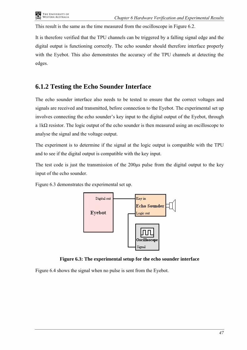
Chapter 6 Hardware Verification and Experimental Results
47
This result is the same as the time measured from the oscilloscope in Figure 6.2.
It is therefore verified that the TPU channels can be triggered by a falling signal edge and the
digital output is functioning correctly. The echo sounder should therefore interface properly
with the Eyebot. This also demonstrates the accuracy of the TPU channels at detecting the
edges.
6.1.2 Testing the Echo Sounder Interface
The echo sounder interface also needs to be tested to ensure that the correct voltages and
signals are received and transmitted, before connection to the Eyebot. The experimental set up
involves connecting the echo sounder’s key input to the digital output of the Eyebot, through
a 1kΩ resistor. The logic output of the echo sounder is then measured using an oscilloscope to
analyse the signal and the voltage output.
The experiment is to determine if the signal at the logic output is compatible with the TPU
and to see if the digital output is compatible with the key input.
The test code is just the transmission of the 200µs pulse from the digital output to the key
input of the echo sounder.
Figure 6.3 demonstrates the experimental set up.
Figure 6.3: The experimental setup for the echo sounder interface
Figure 6.4 shows the signal when no pulse is sent from the Eyebot.

Design of an Active Acoustic Sensor System
48
Figure 6.4: No signal through the echo sounder
What is learnt from Figure 6.4 is that there is a 12.19V signal that is transmitted through the
logic output of the echo sounder. The reason for this is that the signal does not have a
reference. This is unacceptable because the TPU channels can only accept a voltage of 5V at
its pin. To solve this problem, a pull down resistor needs to be used. This is to be placed
between the logic output and the ground of the echo sounder. This properly grounds the signal
and converts it to one that is compatible with the TPU channel.
Figure 6.5: 200µs pulse sent via the digital output, and the transducer is placed in water
Figure 6.5 demonstrates the presence of echoes that are returned to the echo sounder, as
conjectured during the design stage of the echo sounder. These need to be handled by the TPU
channel. The setting of the MAX_COUNT parameter for the TPU as stated in section 5.3.2
should result in only one echo registering with the TPU. The proper reception of pulses
indicates that the digital output is at a sufficient voltage to key the echo sounder circuit.
The echo sounder has been modified according to the tests performed on the echo sounder
interface. In Figure 6.6, a 10kΩ trimpot resistor is used as a pull down resistor. Figure 6.7
shows that the voltage of the logic output of the echo sounder has changed to 4.63V due to the
resistor. This makes it compatible with the TPU channel.

Chapter 6 Hardware Verification and Experimental Results
49
Figure 6.6: the pull down resistor placed between the logic output and the ground
Figure 6.7: Signal when pull down resistor is used
6.1.3 Testing the Combined Interface
The experimental set up for the combined interface is exactly the same as the one used for the
echo sounder interface, except that the logic output of the echo sounder is now connected to
the TPU channels.
Figure 6.8: The experimental setup for the combined interface

Design of an Active Acoustic Sensor System
50
An experiment is conducted to verify that the echo sounder and the Eyebot are correctly
interfaced together.
The test code implemented for this experiment starts the TPU channel and then transmits a
200µs pulse. A key deactivated wait then precedes a display of the time of flight for the signal
on the Eyebot LCD screen.
To test for the functionality of the echo sounder interface, two experiments test for the two
cases which the echo sounder should detect.
The first case is when the echo sounder does not receive any returned pulse. This is simulated
by removing the transducer from the water.
The test verified, as in figure 6.9, that the TPU channel does not receive a second falling edge
meaning that the CPU is not interrupted. A time out needs to be called for this situation and a
maximum time difference recorded by the Eyebot to signify that a real value cannot be
calculated because the surface is either out of range or the transducer is not in the water.
Figure 6.9: Signal at the TPU channel when the transducer is not in the water
The second experiment is to represent a successful transmission of the signal. This is
accomplished by placing the echo sounder in a small container of water. This will result in
significant reverberation, or echoing, which tests to see if the echo sounder can account for
this and only detect the first echo (the first falling edge on the logic output from the echo
sounder).

Chapter 6 Hardware Verification and Experimental Results
51
Figure 6.10: Signal that is received at the TPU channel when the transducer is in the water
Figure 6.10 shows the signal transmitted to the Eyebot from the logic output of the echo
sounder. Notice the multiple secondary echoes that the TPU channel must handle. The
measured time difference from the oscilloscope is compared with the actual time difference
recorded by the Eyebot and displayed on the LCD screen. The time difference as measured
using the oscilloscope is 1.180ms. The time difference recorded by the Eyebot is 4945 counts.
Now each count represents a time of 238.4ns since the smallest resolution is being used (refer
to Appendix B), so the actual time is:
( )sec10179.1time
4945104.238
counts ofnumber time
3
91
−
−
×=
×=
×= cT
This is approximately the same value as the value attained by measuring the time on the
oscilloscope.
The interface can be seen to be functioning according to the specification required. The
signals have been properly matched to suit the voltage requirements of the TPU channels. The
transmitted and received pulses are correctly identified by the TPU channels and the time of
flight can be properly calculated. Thus the interface has been verified to function correctly.
6.2 Determining the Characteristics of Echo Sounding
Once the interface between the Eyebot and the echo sounder is established, it is necessary to
determine the exact physical characteristics of the echo sounder sensor. For these
experiments, the timing out of the channel is not necessary and thus has not been included in
the code set for testing.

Design of an Active Acoustic Sensor System
52
6.2.1 The Linearity of Returns
To verify that the C functions programmed for the echo sounder allowed the Eyebot to
determine the time of flight of the signal, the echo sounder was tested in a long channel of
water in the Hydraulics Laboratory within the university.
The interface was connected, as outlined in Section 6.1.3. To ensure that that there is a
constant voltage supply to both the Eyebot and the echo sounder, both power supplies are
voltage regulated power supplies.
The test script for the Eyebot to test the echo sounder is as follows:
• Initialise the required TPU channel
Then cycle through a loop consisting of the following:
• Start the TPU channel
• Transmit a 200µs pulse from the Eyebot
• Wait until a key is pressed to ensure that an interrupt has occurred
• Display the time of flight on the LCD screen
The loop is to obtain different values for the same location. The results are collected over a
distance from 0.18m to 3.5m and then the values for each distance point is then averaged to
give an average time of flight for the distance point.
Time of Flight for Signal vs distance
0
2000
4000
6000
8000
10000
12000
14000
16000
18000
20000
0 1 2 3 4
Distance to wall (m)
Tim
e of
flig
ht (c
ount
s)
Figure 6.11: Calculated time of flight over a range of distances for the echo sounder

Chapter 6 Hardware Verification and Experimental Results
53
Figure 6.11 is a plot of the experiment, which demonstrates a linear relationship between the
time of flight and the distance to the surface. A statistical analysis of the data shows that
gradient of the function is 5.653x10³ counts/metre.
6.2.2 Calibrating the Echo Sounder
For different types of water and for different temperatures, the speed of sound will vary. It is
vital for the accuracy of the echo sounder that the system be correctly calibrated for the type
of environment in which it will be used.
Given a set of data, like the set in Figure 6.11, it is possible to obtain the speed of sound in the
test medium. Now each data point represents a particular time of flight for a given distance.
Assuming that all the data is linear, then the change in time per unit distance between any two
points equates to the instantaneous rate of change of time with respect to distance.
(6.1)
When this gradient is inverted, it becomes a rate of change of distance with respect to time.
This is the speed of sound in the medium.
(6.2)
So by finding the gradient for the line of regression of the data points, it is possible to
determine the speed of sound in the medium. Not only is this result useful for calibrating the
echo sounder, but it also has applications where the speed characteristic of a particular
environment is required.
To test this theory, the data set in Figure 6.11 is used. The line of regression for the data has a
gradient of:
(6.3)
where ct is the time in counts and ws is the distance to the surface.
This value must be halved to account for the fact that the sound wave must travel the distance
twice, once away from the echo sounder and once returning to the echo sounder.
metrecountsdsdt
w
c /10653.5 3×=
st
dsdt
∆∆
=
dtdscm =

Design of an Active Acoustic Sensor System
54
where rs represents the round trip distance.
Converting the counts to time in seconds using the set resolution of 238.4ns results in the
following:
Inverting this result will give the speed of sound in the medium.
(6.4)
This result is closely approximates the speed of sound in fresh water, which is 1481m/s.
6.2.3 Mean Square Error for the Echo Sounder
Whilst the data appears to be linear, there is some error, even in the averaged data for the plot.
The root mean square (RMS) error for the data from the line of best fit is calculated to be
167.2 counts. The RMS error is calculated by subtracting the predicted value from the
observed value to result in an error, which is then squared. The average of the squared values
is taken to form the mean square value. The RMS value is just the square root of the mean
square value.
The 167.2 counts RMS will result in an error of margin of:
(6.5)
Assuming that the speed of sound in the water is 1484m/s as in equation 6.5.
metrecountsdsdt
r
c /10826.2 3×=
( ) ( )
metredsdtdsdt
r
r
sec/10738.6
104.23810826.2
4
93
−
−
×=
×=
smc
dtdsc
m
rm
/10484.110738.6
1
3
4
×=×
=
=
−
( )
m2
9
1096.2error distance
14842
104.2382.167
sound of speed2
resolutionerrorcount error distance
−
−
×=
××
=
××
=
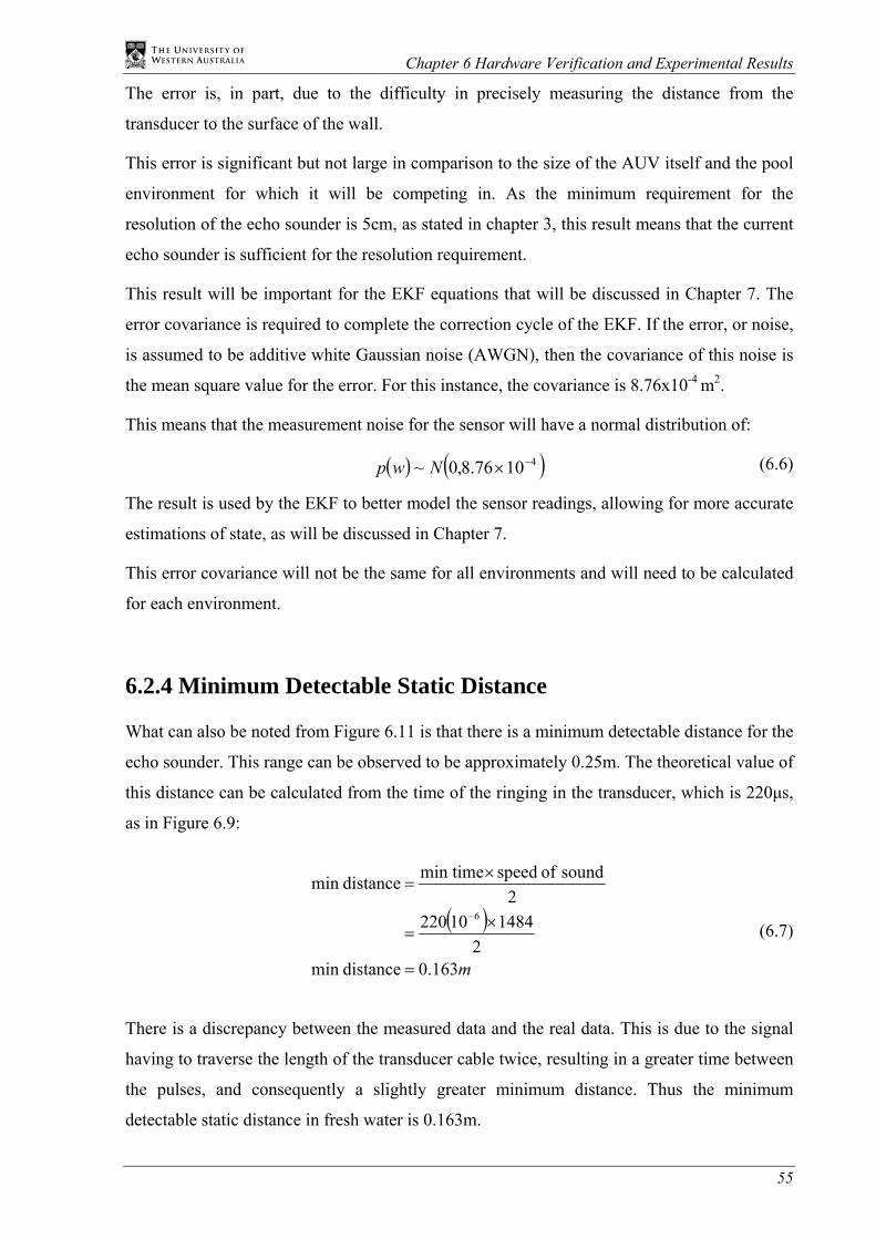
Chapter 6 Hardware Verification and Experimental Results
55
The error is, in part, due to the difficulty in precisely measuring the distance from the
transducer to the surface of the wall.
This error is significant but not large in comparison to the size of the AUV itself and the pool
environment for which it will be competing in. As the minimum requirement for the
resolution of the echo sounder is 5cm, as stated in chapter 3, this result means that the current
echo sounder is sufficient for the resolution requirement.
This result will be important for the EKF equations that will be discussed in Chapter 7. The
error covariance is required to complete the correction cycle of the EKF. If the error, or noise,
is assumed to be additive white Gaussian noise (AWGN), then the covariance of this noise is
the mean square value for the error. For this instance, the covariance is 8.76x10⁻⁴ m2.
This means that the measurement noise for the sensor will have a normal distribution of:
(6.6)
The result is used by the EKF to better model the sensor readings, allowing for more accurate
estimations of state, as will be discussed in Chapter 7.
This error covariance will not be the same for all environments and will need to be calculated
for each environment.
6.2.4 Minimum Detectable Static Distance
What can also be noted from Figure 6.11 is that there is a minimum detectable distance for the
echo sounder. This range can be observed to be approximately 0.25m. The theoretical value of
this distance can be calculated from the time of the ringing in the transducer, which is 220µs,
as in Figure 6.9:
(6.7)
There is a discrepancy between the measured data and the real data. This is due to the signal
having to traverse the length of the transducer cable twice, resulting in a greater time between
the pulses, and consequently a slightly greater minimum distance. Thus the minimum
detectable static distance in fresh water is 0.163m.
( )
m163.0distancemin 2
1484102202
sound of speedmin timedistancemin
6
=
×=
×=
−
( ) ( )41076.8,0~ −×Nwp

Design of an Active Acoustic Sensor System
56
6.2.5 Maximum Detectable Static Distance
For active sonar, according to the formula given in Chapter 2, the detection threshold is the
signal level at which the arriving signal can be detected 50% of the time.
The echo sounder is therefore tested to determine the distance that the device can no longer
detect the arriving signal for 50% of the time. To test for the maximum range of the echo
sounder, the same set up for determining the linearity of the sonar returns was employed.
Starting at a distance of 2m from the surface of the reflecting wall, 500 measurements are
taken to determine whether the signal has been detected for over 50% of the time. Table 6.1
shows the results of the experiment.
Distance
(m) Sample
1 Sample
2Sample
3Sample
4Sample
5Detection
Percentage 2 100 100 97 98 100 99
2.2 100 100 99 98 100 99.4 2.4 100 100 98 98 100 99.2 2.6 99 100 98 98 99 98.8 2.8 99 99 97 98 98 98.2
3 99 97 97 100 97 98 3.2 90 82 87 88 82 85.8 3.4 95 98 99 98 99 97.8 3.6 87 97 90 89 88 90.2 3.8 13 18 18 14 14 15.4
4 14 19 14 19 15 16.2 4.2 1 2 1 1 2 1.4 4.4 0 0 0 0 0 0
Table 6.1: Samples for sonar returns for distances from 2.4m to 3.5m
Table 6.1 shows that the detection of the return signal begins to significantly drop at 3.8m. At
distances longer than 3.8m, the detection begins to drop to 0% making it extremely difficult
for the AUV to detect obstacles.
Figure 6.12 shows the result of Table 6.1 in a graphical form.
The reason for the increasing lack of detection after 3.8m is that the signal becomes
attenuated to a level that is undetectable by the echo sounder. Thus the maximum detectable
static distance is 3.8m in fresh water.

Chapter 6 Hardware Verification and Experimental Results
57
Detection Range for the Echo Sounder
0
20
40
60
80
100
120
0 1 2 3 4 5
distance to the surface (m)
prec
enta
ge d
etec
tion
(%)
Figure 6.12: Detection of an echo for different distances
There are a number of factors that affect the attenuation of the signal in the water. These have
been discussed thoroughly in Chapter 2. The key factors that result in highly attenuated
signals at the receiver are:
• The low intensity of the transmitted signal
• The signal’s susceptibility, at 200 kHz, to losses due to bulk viscosity and absorption
due to relaxation
• The wall’s reflectivity, which will result in only some of the signal being reflected by
the wall whilst the rest is transmitted through the wall
• The natural attenuation of the signal in the medium due to absorption and scattering
This clearly is not the distance that the transducer is capable of achieving and does not meet
the requirement of 5m, as stated in chapter 3. The Navman echo sounder circuit that the
transducer was taken from can achieve a distance of up to 184m. The LM1812 ultrasonic
transceiver chip is capable of depth sounding up to 30m. This clearly indicates that not
enough power is being converted to acoustic energy at the transmitter stage.
6.2.6 Investigation of Signal Transmission Intensity
There were three possible reasons for the lack of signal transmission intensity. These were:
• The key input voltage to the LM1812 chip in not high enough
• The LC resonator has not been correctly tuned to 200 kHz

Design of an Active Acoustic Sensor System
58
• There is a problem with stepping the voltage up to the required level for the
transducer.
One concern was that the 5V pulse from the Eyebot did not have enough voltage to meet the
12V suggested in the LM1812 datasheet [14]. A simple test was conducted to determine if
this may have resulted in a weaker signal transmitted by the echo sounder. The following
circuit is connected between the digital output of the Eyebot and the echo sounder.
Figure 6.13: Driver circuit to increase the voltage at the input of echo sounder
Figure 6.14 is the display of the oscilloscope when no driver is used. Figure 6.15 is the
display when a driver is used. The signals have been inverted so that they can be easily
captured by the oscilloscope. If the amplitude was increased, the transducer should ring much
longer, resulting in the logic output being low for longer. As can be seen in the figures, the
increase in voltage has not resulted in a wider logic output pulse. This means the key input
voltage can be discounted as a factor for the lack of signal intensity.
Figure 6.14: Oscilloscope display for when no driver is used

Chapter 6 Hardware Verification and Experimental Results
59
Figure 6.15: Oscilloscope display for when driver is used
Another possible problem could have been that the LC resonator was not correctly tuned.
Since the resonant frequency of the transducer is 200 kHz, this frequency must be exactly
attained by the LC resonator. To conduct a test for this, the oscilloscope was connected to pin
6 of the LM1812 chip, which is shown in Figure 6.16. Pin 6 is the output signal to the
transducer, from the chip. A pulse was then keyed from the Eyebot.
Figure 6.16: Location of pin 6 and transformer windings on the circuit diagram [14]
Figure 6.17 shows the result of the experiment. The measured frequency of the output from
the LM1812 chip is exactly 200 kHz, which indicates that the LC resonator has been tuned
correctly.

Design of an Active Acoustic Sensor System
60
Figure 6.17: Frequency of LM1812 output
The final possible cause for the lack of signal intensity is that the voltage signal to the
transformer, which drives the transducer, is not stepped up to the right amplitude. If there is a
problem at the step-up transformer stage, then there will not be significant lack of signal
intensity for transmission. The test was conducted using the following procedure.
• Connect the oscilloscope across the primary windings of the transformer, shown in
Figure 6.16, and key a pulse from the Eyebot to determine the peak-peak voltage (Vp-
p) of the input to the transformer. Repeat this, connecting the oscilloscope across the
secondary windings of the transformer to determine the Vp-p of the output of the
transformer.
Figure 6.18: Peak-peak voltage of transformer input
Figure 6.19: Peak-peak voltage of transformer output

Chapter 6 Hardware Verification and Experimental Results
61
Figures 6.18 and 6.19 show the observations of this experiment. As can be seen from the
figures, there voltage has only been stepped up from 20.63Vp-p to 30.78Vp-p. However, the
transformer has been designed with a turns ratio of 4.5:1. This means that the voltage should
be stepped up by a factor of 4.5. This clearly is not the case.
The problem may be that the transformer does not properly match the source impedance to the
load impedance of the transducer at 200 kHz. When these are matched, then there is
maximum power transfer to the transducer. If the load and source impedance are given as:
(6.8)
And the transformer equations are:
(6.9)
where N1 and N2 are primary and secondary windings respectively, then the impedances can
be matched by adjusting the windings to suit the following equation:
(6.10)
To solve this impedance mismatch problem, the transformer’s windings need to be adjusted
so that equation 6.10 is correctly met.
There are two other solutions possible that target the intensity of the signal, one implemented
at the transmitter and one implemented at the receiver. The first is to develop a pulse amplifier
that will increase the intensity of the signal at the transmitter. The second solution is to have a
larger gain at the receiver to detect the smaller intensity signals. This can be achieved through
a time variable attenuator. Both of these will be discussed in Chapter 8.
6.2.7 Time Redundancies for a Simple Fault Tolerant System
For the data seen in Table 6.1, it is clear that a fault tolerant system needs to be implemented
to ensure that there is minimal probability of erroneous readings from the sensor.
1
1
2
2
IVR
IVR
S
L
=
=
21
21
22
11
INNI
VNNV
=
=
LS RNNR
2
2
1⎟⎟⎠
⎞⎜⎜⎝
⎛=

Design of an Active Acoustic Sensor System
62
A simple system is implemented for the echo sounder based on the mid-value select method
for choosing data points. The mid-value select method selects the median value from three
readings to attempt to eliminate the chance of returning an outlying data point. In this case,
the three values will be consecutive readings from the echo sounder. This will utilise the time
redundancies to improve the estimate for distance.
The problem with a mid value select method is that the data returned by the echo sounder will
have outliers lower than the true value. A much better approach is to choose the maximum
from a set of three data points. This, too, is flawed in that it still may be possible to achieve an
outlier above the true value.
A new method for fault tolerance is proposed. This involves the use of a pre-filter to remove
most of the lower outliers. The pre-filter is just the maximum value from a number, selected
by the user, of consecutive readings from the echo sounder. This is performed three times to
obtain three maximum values. The median value of these three values is then selected to
ensure that any higher outliers are not selected.
Distance
(m) Samples Detection
Percentage 2 10232 10242 10241 10231 10228 100
10243 10240 10245 10245 10228 2.2 11447 11449 11448 11449 11465 100
11449 11449 11449 11450 11449 2.4 12744 12747 12801 12745 12746 100
12745 12799 12746 12746 12746 2.6 13807 13828 13824 13810 13822 100
13809 13810 13822 13808 13809 2.8 14968 14967 14967 14968 14968 100
14966 14968 14968 14968 14966 3 16104 16106 16116 16103 16103 100
16102 16103 16102 16102 16102 3.2 17251 17254 17250 17251 17253 100
17256 17250 17249 17250 17251 3.4 18352 18353 18356 18352 18350 100
18352 18352 18354 18351 18349 3.6 19457 19424 19424 19423 19423 100
19423 19422 19437 19412 19423 3.8 20579 20571 20581 20578 20580 100
20580 20578 20579 20576 20575 4 21606 21610 21608 21586 21620 60
1724 1724 21607 1699 1991 4.2 22791 22763 11442 22742 22756 90
22767 6906 22742 11668 22743 4.4 1661 1672 1671 1689 1676 0
1656 1724 1664 1676 1674 Table 6.2: Samples of sonar returns using extended mid-value select method

Chapter 6 Hardware Verification and Experimental Results
63
Table 6.2 shows the percentage detection over the range of distances measured for Table 6.1
using a pre-filter of size 3. This means that a maximum is chosen from three consecutive
readings. It can be seen that, whilst the fault tolerance implemented does not increase the
detectable range by much, it allows a virtually flawless detection rate over the entire
detectable range.
This method of fault tolerance may take approximately nine times longer to process than just
obtaining one reading, but it allows sonar returns to be more continuous, which is essential for
navigational purposes. The pre-filter can be shortened if less time for processing is necessary.
The form of fault tolerance implementation only has significant merit in the static cases, as is
discussed in the next section.
6.3 Performance of the Sensor in a Dynamic Environment
The final part of this chapter deals with the performance of the echo sounder at tracking
objects that move, or when the echo sounder is moving. Up until now, the tests performed on
the echo sounder involved static experiments where the echo sounder was placed a certain
distance from a wall and the time of flight measured.
This final experiment deals with a fixed transducer position in the water, with the transducer
pointed into free space. A moving wooden rod is placed in from of the transducer and is
moved back and forth in front of the transducer. The distance measurement is recorded and
stored in an array, ready for uploading to a PC upon completion of the measurement stage.
The points are then plotted on to a graph.
A new code set has been written for this experiment with the timing out of the channels, as is
seen in the flow chart in Chapter 5, accounted for in assembly and C functions. Figures 6.20
and 6.21 show the graphs of the experiment. The data set is collected using the modified mid-
value select method.

Design of an Active Acoustic Sensor System
64
Tracking the Stick 1
0
1
2
3
4
5
6
0 50 100 150 200 250
time (samples)
dist
ance
(m)
Figure 6.20: Distance wooden rod is from sensor over time
Tracking the Stick 2
0
1
2
3
4
5
6
0 200 400 600
time (samples)
dist
ance
(m)
Tracking the Stick 3
0
1
2
3
4
5
6
0 200 400 600
time (samples)
dist
ance
(m)
Figure 6.21 a) & b): Measuring distance from the rod over 500 time samples

Chapter 6 Hardware Verification and Experimental Results
65
What can be seen from these graphs is that even with the implementation of a simple fault
tolerant system, it is not possible to achieve zero errors in measurement.
The reason for this is that the obstacle is moving creating turbulence in the water. This
turbulence will distort the echo’s frequency by adding random noise to the signal. As the
circuit is tuned to 200 kHz, it will not be able to detect a significant distortion in frequency.
Thus for the AUV to detect a wall or obstacle, it must be travelling at low speeds. This is
ensured on the current AUV as the thrusters only allow low velocities. At the speeds the AUV
will be travelling at, there should be minimal turbulence in the water. However, care must be
taken to ensure that the sensors are not placed near areas of significant turbulence on the
AUV, such as near the thrusters.
There is also another reason for the erroneous readings. The echo signal is subject to a
phenomenon called the Doppler Effect. The Doppler Effect is when the observed frequency of
the signal changes from the source frequency because the object is moving away or towards
the source. The frequency of the observed signal becomes:
(6.11)
Since the Doppler Effect occurs both towards the rod and back to the sensor the formula can
be written as:
(6.12)
However, since the speed of the AUV will be very small with respect to the speed of sound,
this effect is minimal in comparison to the effect that the turbulence has on the amount of
erroneous readings.
At slow speeds, like in Figure 6.20, the sensor can track the rod well, with errors only when
the rod is closer than the minimum detectable distance. This is compared with Figure 6.21
where the rod was moved much quicker. More errors are introduced as the sensor cannot
detect the frequency properly.
An attempt is made to reduce the number of higher outliers by adjusting the modified mid-
value select method. For this experiment, 10 samples are taken and the 7th sample in
ascending order is taken as the estimated value. A) and b) of Figure 6.22 demonstrate the
results of such an experiment.
sound
source
vv
ff=
∆
sound
rod
vv
ff 2=
∆

Design of an Active Acoustic Sensor System
66
Tracking the Stick DMVS 1
0
1
2
3
4
5
6
0 200 400 600
time (samples)
dist
ance
(m)
Tracking the Stick DMVS 2
0
1
2
3
4
5
6
0 200 400 600
time (samples)
dist
ance
(m)
Figure 6.22: 7th value select method on the tracking of a wooden rod
As can be seen from the plots, outliers from above the true value are removed, but are then
replaced by outliers from below the true value. What this means is that it is impossible to
remove all the outliers from being detected using this method of fault tolerance. However,
using the earlier modified fault tolerance method, the percentage error is 20%, as opposed to
40%, for the latter, to 20%.
The errors may be reduced partially by investigating the population of data points to
determine where the data, which is within 10% of the true value, lies in relation to the ordered
data set. For example, if the investigation found that this data lies in the 80th percentile, then
10 sample points can be taken and sorted in ascending order, and the 8th data point will be the
estimate of the data. This is an area for future investigation.
Obviously, the more data points collected, the better the robustness of the system, but this will
result in a slower data rate. 10 sample points will result in a data rate of approximately 10Hz,
which is the minimum requirement for this project, and thus should not be exceeded.

Chapter 6 Hardware Verification and Experimental Results
67
6.4 Summary of Experimentation
Some important results have been obtained through experimentation with the echo sounder
unit. These results are:
• Verification of the Eyebot interface to the echo sounder to be completely functional
• Verification of the linearity of the sonar returns as a function of distance
• Establishment of a method of calibrating the echo sounder to the speed characteristics
of the medium
• Determination that the mean square error for static measurements of distance in fresh
water is 2.96cm. This falls within the required resolution of 5cm, as stated in Chapter
3
• Determination that the minimum detectable distance in the test environment is 0.25m.
• Determination that the maximum detectable distance using the current circuit in fresh
water is 3.8m. This does not meet the minimum 5m requirement. However, the
recommendations made should allow the sensor to achieve this target
• Knowledge that the lack of detection range is due to the transformer mismatching the
transducer and source impedance, resulting in a lack of transmitted signal intensity
• Implementation of a simple fault tolerant system using time redundancies to improve
the robustness of the sensor for static distance measurements
• Knowledge of sensor degradation when dynamically measuring distances
• Knowledge that errors in dynamic distance measurements cannot be completely
removed using time redundant fault tolerance but can be decreased by modifying the
mid-value select method
• Knowledge that at low speeds, turbulence and the Doppler Effect are minimised and
thus the sensor is capable of tracking obstacles effectively


69
7 Navigation Using the Sonar Sensors
Navigation is an important part of an AUV’s autonomy. In order to be completely
autonomous, the AUV must successfully navigate a path to a target or goal, using only its
sensors. Since sound is the best form of sensing in water over distances, it is the medium of
choice for many applications. Since an echo sounder has been implemented, it is possible to
perform such tasks as wall following and obstacle avoidance. This section will discuss the
development of extended Kalman filter equations and control equations that can be used with
the AUV in conjunction with the sonar sensors.
7.1 Active Sonar Application
For an AUV, the wall following problem is a key aspect of its navigation. In an unknown
environment, when a new wall is found, a search algorithm is usually implemented so that the
autonomous vehicle can collect information about the nature of the wall, such as orientation,
position and length. The only method of detecting a wall is by active sonar.
The wall following problem first needs to be formulated before a set of control equations can
be derived for the AUV. These equations can then be used to create the extended Kalman
filter equations.
7.1.1 The Wall Following Problem
The AUV is required to follow the wall of a pool as it navigates a full circle about the pool.
This means that the AUV needs to remain a constant distance from the pool’s edge whilst
maintaining a constant velocity. The AUV has a compass, a velocity sensor and an echo
sounder with which to complete the task.

Design of an Active Acoustic Sensor System
70
Figure 7.1: The wall following problem
Using the problem formulation from Bemporad et al [24] and Figure 7.1, a set of equations
for the wall following task is defined.
From the information from these sensors, the position state of the AUV can be determined
using the following equations:
(7.1)
where v is the speed of the AUV whilst ω is the angular velocity of the AUV.
What is required is the design of the feedback controller that will allow the AUV to move at a
constant velocity at a constant distance from the wall of the pool.
Assuming that the wall is considered straight and infinite, the wall can be determined by a line
passing through a point.
ωθ
θθ
=
==
&
&
&
sincos
vyvx

Chapter 7 Navigation Using the Sonar Sensors
71
where ( )ww yx , is a point on the wall. The equation for the wall can be written as:
(7.2)
The zero represents the distance from the wall, thus all points satisfying this equation is on the
wall.
The equation for the distance to the wall can thus be written as:
(7.3)
The distance that the echo sounder’s transducer will be from the wall is calculated as:
(7.4)
where ),( offyoffx dd is the position of the transducer with reference to the centre of the AUV.
7.1.2 Constraints of the System
Now, the AUV is not capable of high speeds, which means that there is a speed constraint on
the controller that will be used. The benefit of this is that low velocities enable a control
system that is more robust. This places the constraint on the motors of the AUV:
(7.5)
where 2α is the distance between the forward thrusters, Ωmax is the maximum speed attained
by each of the thrusters.
There is also a constraint on the orientation of the AUV from the surface of the wall. Because
the echo sounder has a finite beamwidth in which it can detect an echo return, in theory, AUV
cannot tilt more than half the beamwidth of the echo sounder, as can be seen in Figure 7.2.
This leads to the constraint that:
( ) ( ) γγγγγ
γ
sincoscossintan
tan
ww xxyyxy
dxdy
xy
dxdy
−=−
=∆∆
=
=∆∆
=
( ) ( ) 0sincos =−−− γγ ww xxyy
( ) ( ) γγ sincos ww xxyyd −−−=
( ) ( ) γγ sincos woffxwoffy xdxydyr −+−−+=
maxΩ≤±αωv

Design of an Active Acoustic Sensor System
72
(7.6)
where φ is the half beamwidth of the echo sounder.
Figure 7.2: No returned echo at an angle greater than half the beamwidth
7.2 The Extended Kalman Filter
The sensors on the AUV are always prone to measurement error. This means that in practice,
the actual coordinates of the AUV will never be accurately known. The only way to localise
the AUV is to use the noise corrupted sensors to provide a distorted view of the environment.
The magnetic compass on the AUV is the most classical absolute orientation sensor. However
the precision that can be obtained is usually low and it can be strongly affected by external
disturbances. When an extra magnetic field, for example motors and electrical equipment, is
present, the precision of the compass can be very bad. This is the case with the AUV, where
the hard disk for the onboard computer is in close proximity to the compass.
The velocity meter is, at best, tolerable in determining the speed of the AUV. It is based on a
paddle wheel with two magnets on the circumference to trigger a pulse. The velocity is
calculated by counting the number of pulses per unit time. The resolution for this device is
poor at low velocities as the resolution is large with respect to lower velocities due to
quantisation.
Because information from sensors is incomplete, erroneous and uncertain, it is essential that
the system fuse redundant information from multiple sensors. This is the acquisition of data
that, in part, measures the same quantities as the other data, and combines these measurements
to determine a more accurate view of the environment.
φγθ ≤−

Chapter 7 Navigation Using the Sonar Sensors
73
The extended Kalman Filter (EKF) is a method of accomplishing the fusion of data from
different sensors. The EKF is used to obtain an estimate of the position state from an estimate
of the distance from the wall. The sensor will use the error in distance reading to correct the
predicted position state.
7.2.1 The Control Equations
Firstly, a set of control equations is required to give an indication of the system. The position
state is the variable to be estimated by the EKF. For the position state:
(7.7)
The input of the system is:
(7.8)
The control equation is therefore given as:
(7.9)
(7.10)
It is clear why the EKF needs to be applied here. The control equations for this system are
non-linear and thus cannot be filtered using the standard Kalman filter.
As defined in Chapter 2, the Jacobian matrices of partial derivatives A and H need to be
calculated in order to proceed with the filtering process. These matrices are calculated as
follows:
(7.11)
( )( )( )( )⎥
⎥⎥
⎦
⎤
⎢⎢⎢
⎣
⎡=
kkykx
kXθ
( )( )( )
( ) ⎥⎥⎥
⎦
⎤
⎢⎢⎢
⎣
⎡=
kkvkv
kUω
θθ
sincos
( )( ) ( )( ) ( )( ) ( )
( )kETkk
TkvkyTkvkx
kX X
c
c
c
+⎥⎥⎥
⎦
⎤
⎢⎢⎢
⎣
⎡
+−+−+−
=ωθ
θθ
1sin1cos1
( ) ( ) ( )[ ] ( ) ( ) ( )kxdydkxkykz woffxwoffy ξγγγγ +−+−+−= sincossincos
( )( )
⎥⎥⎥
⎦
⎤
⎢⎢⎢
⎣
⎡ −=
100cos10sin01θθ
c
c
TkvTkv
A

Design of an Active Acoustic Sensor System
74
(7.12)
(7.13)
(7.14)
where W and V are identity matrices because it is assumed the noise is white and additive.
7.2.2 Filter Predict and Correct Cycle
The filtering process then proceeds with the time update equations, which predict the position
state variable and the error covariance matrix, using the compass and the velocity meter.
These are based on the equations in Section 2.6.
(7.15)
(7.16)
Once these have been calculated, the two variables can then be corrected using the returns of
the echo sounder. This must be preceded by the adjustment of the Kalman gain. In equation
7.17, the error covariance, R(k), is the mean square error calculated in Chapter 6.
(7.17)
[ ]0cossin γγ−=H
( )( ) ( )( ) ( )( ) ( ) ⎥
⎥⎥
⎦
⎤
⎢⎢⎢
⎣
⎡
+−+−+−
=−
c
c
c
TkkTkvkyTkvkx
kXωθ
θθ
1ˆsin1ˆcos1ˆ
ˆ
( )( )( ) ( )
( ) ( ) ⎥⎥⎥
⎦
⎤
⎢⎢⎢
⎣
⎡
+⎥⎥⎥
⎦
⎤
⎢⎢⎢
⎣
⎡
−−
⎥⎥⎥
⎦
⎤
⎢⎢⎢
⎣
⎡ −=−
2
2
2
000000
1cossin010001
1100
cos10sin01
θσσ
σ
θθθθ
y
x
cc
c
c
TkvTkvkPTkv
TkvkP
⎥⎥⎥
⎦
⎤
⎢⎢⎢
⎣
⎡=
100010001
W
⎥⎥⎥
⎦
⎤
⎢⎢⎢
⎣
⎡=
100010001
V
( ) ( ) [ ] ( ) ( )
1
0cossin
0cossin0
cossin
−
−−
⎟⎟⎟
⎠
⎞
⎜⎜⎜
⎝
⎛+
⎥⎥⎥
⎦
⎤
⎢⎢⎢
⎣
⎡−−
⎥⎥⎥
⎦
⎤
⎢⎢⎢
⎣
⎡−= kRkPkPkK γ
γγγγ
γ

Chapter 7 Navigation Using the Sonar Sensors
75
(7.18)
(7.19)
The filtering then cycles back to the prediction stage and the filtering begins again.
7.3 The Feedback Controller
When the position state has been calculated, then the values can be fed back into the
controller for the system. Using the control laws provided by Bemporad et al [24], a feedback
controller is made. These are:
(7.20)
The µ is used to ensure that the speeds for the thrusters do not exceed their maximum speed.
As long as maximum speed of the thrusters is never exceeded, this value can be assumed
unity.
The desired velocity is a constant value and does not need to be calculated. The desired
angular velocity, however, can be calculated using the following [24]:
(7.21)
This controller is basically a modified proportional controller which takes into account the
error for distance to the wall and the orientation error relative to the wall simultaneously. The
beta values are set by the user experimentally to achieve the best results for the particular
application.
( ) ( ) ( ) ( ) ( ) ( )[ ]γγ sincosˆˆwoffxwoffy xdxydykzkKkXkX −++−+−+= −
( ) ( )[ ]( ) ( )−−−= kPkKIkP 0cossin γγ
des
desvvωµω
µˆ
ˆ−=
=
( ) ( ) ( )γθβββ
ω −−+−−
−= ˆtanˆˆ 210
desdes
desdes dd
vdd


77
8 Future Work
The work that has been completed in this thesis provides the basis for future research and
development of sonar systems. There are a number of key areas that can be developed in
further work within the Mobile Robotics Lab. These key areas are:
• Developing a pulse amplifier that will correctly reach the desired range of the sonar
system
• Developing a time variable attenuator to assist in better detection with the echo
sounders
• Research into the feasibility of using a receiver based on the current echo sounder to
be the base of a passive sonar array
• Implementing a control system in practice that will utilise the EKF to allow the AUV
to perform the tasks of wall following and investigate the possibility of performing
simultaneous location and mapping with the AUV
• Further investigate the parameters of the echo sounder to provide a more realistic
model of the sonar system.
8.1 Improving the Echo Sounder Design
Two key design changes to the current echo sounder circuit are suggested for future work to
improve the performance of the system over the current one.

Design of an Active Acoustic Sensor System
78
8.1.1 The Pulse Amplifier
As discussed in Chapter 6, the power output from the transducer is not sufficient to perform
echo sounding over the required minimum of 5m.
One recommendation to increase the amount of power that is outputted from the transducer is
to increase the voltage across the transformer of the circuit. Figure 8.1 depicts a pulse
amplifier [14]. This pulse amplifier attempts to increase the signal strength using a transistor
combined with a transformer. The transistor allows for most of the supply voltage, V+, to drop
across the primary of the transformer when it is switched on. V+ can be increased to allow a
much higher voltage to fall across the primary windings of the transformer. Since the
transformer is a step-up transformer, the voltage across the secondary winding is increased by
the turns ratio of the transformer. This will allow for a greater amplitude signal that will be
able to travel further.
Figure 8.1: The pulse amplifier [14]
However, care must be taken to design a pulse amplifier that only increases the range of the
sensor to between 5 metres and 10 metres. This is just to enable the signal to attenuate fast
enough to allow consecutive readings to occur rapidly. The current system has a range of less
than 5 metres and has a sounding period of less than 6.67ms. Thus, the current time out for
the echo sounder waiting for a sonar return is 10ms which can easily be accomplished by the
ROBIOS function, OSWait(1). This allows approximately 100 measurements to occur each
second for virtually continuous measurements.
8.1.2 The Time Variable Attenuator
A second design change involves the use of a time variable attenuator to improve the
performance of the current system.

Chapter 8 Future Work
79
With the use of a single transducer, as in the current system, the echo sounder is more
susceptible to ringing from the transducer. While the transducer is ringing, the system cannot
detect any echoes, limiting the minimum detectable distance.
Currently, it is not possible to decrease the minimum detectable distance because the
transducer’s ringing saturates the receiver. This is not a problem with the existing system
because the sensors will be offset by approximately the minimum detectable distance from the
extremity of the AUV.
If the minimum distance is found to be too great, it can be decreased using a circuit provided
by National [14]. The circuit is called a time variable attenuator.
Figure 8.2: Time variable attenuator [14]
The time variable attenuator works by changing the gain of the receiver from a minimum to a
maximum over a small period of time. When the transmission pulse comes from the
microcontroller, it turns the field effect transistor off, causing the gain of the receiver to
become very small. This is beneficial because, at this time, the transducer’s ringing is so
intense that it saturates the receiver, preventing it from detecting echoes. Since the close
echoes are much stronger in intensity than the ringing, they can still be detected even when
the gain is near zero. Over time, the gate voltage becomes higher and the attenuation of the
receiver signal becomes much smaller. This is also beneficial as the far-range echoes become
significantly less intense and require a much larger amplification than the close range echoes.
These far-range echoes take longer to return and are thus amplified greater with the time
variable attenuator. Thus by implementing a time variable attenuator, the detectable range is
increased to include much smaller and larger values.

Design of an Active Acoustic Sensor System
80
8.2 Future Research
Some key areas are identified for possible future research in the AUV field. These areas
include the development of a passive sonar system, the testing of control systems using
simulations of the AUV, and researching the sonar system to provide a more realistic model
of the system for use in simulations and calculations.
8.2.1 Designing a Passive Sonar Array
There are times when a passive sonar system is required. For example, in competition, the
passive sonar has been used to locate a recovery zone marked by an acoustic beacon. In
general underwater applications, an acoustic beacon can be used on a lost submerged vessel
that the AUV may be required to find. Methods of developing a passive sonar array need to be
investigated for such situations.
One simple method of designing a passive sonar unit is to use the receiver of an active sonar
unit attached to an omni-directional hydrophone, which is basically an underwater
microphone, instead of a directional transducer. The feasibility of using a device similar to the
current unit for passive sonar detection can be investigated in future. If the device is feasible,
research can be undertaken into passive sonar detection, such as in Appendix C.
8.2.2 Testing the Control System
The EKF is an extremely powerful tool in the navigation of the AUV using sensors. As is
stated in Chapter 7, the EKF fuses redundant sensor readings to determine a better localisation
of the AUV in its environment.
The EKF equations presented in this thesis can be used as the basis for testing the
effectiveness of the EKF in navigating an AUV around the edge of a pool environment or an
unstructured underwater environment.
These tests can be performed in software before implementing them in hardware. With the
onset of a simulation for the AUV available for use within the university, it would be possible
to test complex algorithms on realistic models of the AUV and its complement of sensors to
see if it is possible to use a particular type of control system for the AUV, before committing
any finance towards a hardware system. Models can be created to simulate any hardware that

Chapter 8 Future Work
81
is available on the market, so that comparisons can be made to determine the optimum type of
hardware system.
8.2.3 Developing a Better Model for the Sensor System
The parameters discovered in this thesis provide some insight as to how the acoustic sensor
system behaves on the AUV. A model using this information can be built into a simulation to
determine the extent of its effectiveness as a sensor system on the AUV.
Further research into the modelling of the sensor system will allow a more realistic model to
be achieved, meaning that the simulation software will be able to provide a more accurate
representation of how the AUV will behave in a real environment.


83
9 Conclusion
The design of an active acoustic sensor system is presented in this thesis. There has been
much work accomplished in the design phase of this project.
Much time was spent researching different approaches to solving the problem of designing a
new echo sounder circuit that could fulfil the requirements set out in Chapter 3 and ensure the
design’s best chance of success. After a design was chosen, it needed to be quickly converted
into a physical design to initiate functional testing of the echo sounder and establish the
suitability of the new circuit as a part of an active sonar system.
9.1 Outcomes of the Project
There are a number of contributions that were made in this project, outlined in the sections
below.
9.1.1 Designing the Echo Sounder Circuit
Many alternatives were considered in the design stage of prototyping a new echo sounder
circuit. This included AM transceivers and ultrasonic switches. All these devices had a similar
form of operation to an actual echo sounder. However, these designs did not meet the
requirements for the project as most of these contained many components which resulted in
poor SNR performance. They also used a dual transducer system, rather than a single
transducer system. The chosen design was a circuit that contained a dedicated ultrasonic
transceiver chip that could perform the entire signal transmission and detection. This allowed
for the number of components to decrease on the circuit board and meant that a single
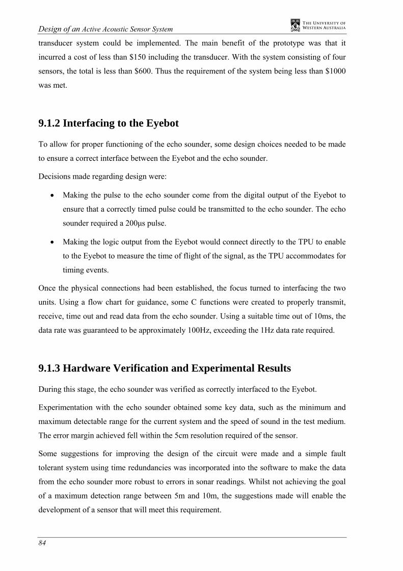
Design of an Active Acoustic Sensor System
84
transducer system could be implemented. The main benefit of the prototype was that it
incurred a cost of less than $150 including the transducer. With the system consisting of four
sensors, the total is less than $600. Thus the requirement of the system being less than $1000
was met.
9.1.2 Interfacing to the Eyebot
To allow for proper functioning of the echo sounder, some design choices needed to be made
to ensure a correct interface between the Eyebot and the echo sounder.
Decisions made regarding design were:
• Making the pulse to the echo sounder come from the digital output of the Eyebot to
ensure that a correctly timed pulse could be transmitted to the echo sounder. The echo
sounder required a 200µs pulse.
• Making the logic output from the Eyebot would connect directly to the TPU to enable
to the Eyebot to measure the time of flight of the signal, as the TPU accommodates for
timing events.
Once the physical connections had been established, the focus turned to interfacing the two
units. Using a flow chart for guidance, some C functions were created to properly transmit,
receive, time out and read data from the echo sounder. Using a suitable time out of 10ms, the
data rate was guaranteed to be approximately 100Hz, exceeding the 1Hz data rate required.
9.1.3 Hardware Verification and Experimental Results
During this stage, the echo sounder was verified as correctly interfaced to the Eyebot.
Experimentation with the echo sounder obtained some key data, such as the minimum and
maximum detectable range for the current system and the speed of sound in the test medium.
The error margin achieved fell within the 5cm resolution required of the sensor.
Some suggestions for improving the design of the circuit were made and a simple fault
tolerant system using time redundancies was incorporated into the software to make the data
from the echo sounder more robust to errors in sonar readings. Whilst not achieving the goal
of a maximum detection range between 5m and 10m, the suggestions made will enable the
development of a sensor that will meet this requirement.

Chapter 9 Conclusion
85
9.1.4 The Wall Following Algorithm
The EKF is used with a control system for a mobile robot designed by Bemporad et al (2000)
to design a set of EKF equations and control equations for the AUV. These can be used, once
the control system of the AUV is fully developed, to navigate the AUV around the edge of a
pool.
9.2 Final Word
The goal of this project was to design a low active acoustic sensor system for an AUV. The
design was accomplished, with effective system functioning and establishment of control
equations to use with the system. Further research needs to be conducted to improve the range
and modelling of the echo sounder system. However, this project has provided a platform on
which future research can build on improving AUV performance in a number of different
environments.


87
Appendix A: The Time Processor Unit
A.1 Channel Control
Function code
Host service request code
Host Sequence code
0xA 1 = Initialise channel
0 = No link, single capture 1 = No link, continuous 2 = Link channels, single capture 4 = Link channels, continuous
Table A.1: TPU code options [22]
• The interrupt enable must be set to 1 if the TPU channel is to interrupt the CPU
• The interrupt status register indicates when an interrupt has occurred for the channel
and does not need to be set
• The channel priority register is the register that begins operations for the channel and
must be set last. The code for it determines the priority at which it is serviced by the
TPU. This ranges from 0 to 4. If the register is zero, this means the channel is not on.
Apart from the interrupt status register, all the registers need to be set before the channel can
operate properly.

Design of an Active Acoustic Sensor System
88
A.2 Parameter RAM
The following is what is required in the parameter RAM in order to allow the ITC function to
operate properly.
Parameter Value Meaning Inputs: CHANNEL_CONTROL Bits[1:0] 11 Input channel Bits[4:2] 000
001 010 011
Do not detect transition Trigger on rising edge Trigger on falling edge Trigger on either edge
Bits[8:5] 00xx 000x 001x
Timer on input channel Reference timer 1 Reference timer 2
MAX_COUNT 0 < N ≤ 0xFFFF Number of events to count Table A.2: Parameter RAM for ITC [22]

89
Appendix B: The Timer Frequencies
The table defines the possible clock frequencies that are available to the timer used for the
TPU [Harman, 1991]. This is based on a 16.78MHz system clock. The resolution is the clock
signal’s period used for clocking the timer. As the distances for the echo sounder range
exceed the 5m to 10m range boundary set for the project, the time range may also need to
increase. This will mean that the resolution will not be as fine. The 31.25ms range will be
necessary when the distance range is between 11.7m and 23.4m.
Frequency Resolution Range 4.19MHz 238.4ns 15.6ms
2.097MHz 476.8ns 31.25ms 1.049MHz 953.7ns 62.5ms 0.524MHz 1.91µs 125ms 262.1kHz 3.81µs 0.25s 131.1kHz 7.63µs 0.5s 65.53kHz 15.3µs 1.0s
Table B.1: List of TPU timer frequencies, and corresponding resolutions and ranges [22]


91
Appendix C: Passive Sonar Application
The possibility of being able the convert the active sonar unit to a passive sonar unit, by
blanking out the transmitter, enables the development of passive sonar applications. The main
use for passive sonar is the detection of a sound source underwater. The advantages for this
approach are:
• The sensor can detect a sound source from twice the distance that an active sonar unit
can, due to the fact that the signal must be sent out and reflected before it is detected,
reducing the range of the active sonar. This is assuming the same signal intensity is
transmitted from both.
• The location of the sensor cannot be discovered when using passive sonar, because the
sensor does not emit a sound. When a sensor emits a sound, it is possible to locate the
sensor using an array of passive sonar. This is why passive sonar is used in the
military.
It is, therefore, beneficial to research passive sonar detection.
C.1 Time Delay Estimations
The main method of detecting the DOA of a signal is by using the time delays between
sensors and the geometry of the sensors to triangulate the DOA. With the use of a system,
implemented with sensors similar to the ones for this project, it is easy to determine an
approximate time delay between sensors.
In order to triangulate the DOA of a signal in 3 dimensions, 3 time delays are required. This
will mean that at least 3 sensors will need to be placed in the array. However, the arrangement
of 3 sensors means that the sensors will have to be timing continually as there is no way of
determining when a signal will be approaching.
A much more effective method is to use four sensors. This system will rely on a trigger
system to activate the sonar array. Initially, also the sensors will be set to detect a signal of the
correct frequency. This will not require any CPU processing time as the TPU is a separate
module from the CPU on the Motorola 68332 microcontroller. Once a signal impinges on the
first sensor in the array, the three other sensors’ timers are triggered, using the linking
capabilities of the TPU channels, to determine how long it takes for the signal to arrive at

Design of an Active Acoustic Sensor System
92
each individual sensor. This is shown in Figure C.1. The red sensor is the sensor that detects
the signal, and the other three green ones must time how long it takes for the signal to arrive.
Figure C.1: Signal impinging on the first sensor of passive array
For a much more robust method of detecting the time delays between sensors, a digital signal
processor (DSP) is required. The method behind this is to digitalise the signal that is being
received by the sensors. It is accomplished by using an ADC.
The digitalised signal is then sent to the central processor where the signal is cross correlated
with a neighbouring sensor’s signal to determine the time delay between the two sensors. A
cross correlation is a function that reaches its maximum value when the phase or time delay
between two signals is matched. To perform a cross correlation on two signal sequences, the
best approach is to perform a fast Fourier transform (FFT) on both of them, multiply the
sequences together and then inverse FFT the resultant sequence [2], as this is computationally
less expensive.
(C.1)
By analysing the resultant cross correlation sequence for the maximum value, the time delay
between the two sensors is discovered.
( ) ( ) ( )
( ) ( )[ ]
( ) ( )[ ] ( )[ ][ ]kyFkxFFN
R
fYfXFN
kykxN
R
xy
N
kxy
1
1
1
0
1
*1
1
−
−
−−
=
=
=
+= ∑
λ
λλλ

Appendix C Passive Sonar Detection
93
This method is far more robust then the first method, that uses the echo sounder as a receiver
to detect time delays, because this can be used when the SNR at the sensors is not very high.
The cross correlation give the best estimate of the time delay in a noisy environment, whereas
the echo sounder receiver will not be able to detect the signal and thus cannot provide a TDE
for noisy environments. This does come at a cost as the DSP systems are much more
expensive and difficult to build.
C.2 Direction of Arrival Calculation
Once the TDEs are determined for the sensor array, then the DOA can be calculated, using the
TDEs and the geometry of the sensors.
The time delay direction finding (TDDF) algorithm by Berdugo et al [4] is the easiest method
for determining the DOA.
Now the sensor positions can be represented by:
(C.2)
The differential time delays can be placed in a vector:
(C.3)
And the DOA vector is:
(C.4)
The time delay between two sensors can be determined as the projection of the distance vector
between the two sensors onto the incoming wave vector, k, divided by the speed of sound, c.
(C.5)
[ ]iiii zyxr =r
ijij ττττττ
τ −≡⎥⎥⎥
⎦
⎤
⎢⎢⎢
⎣
⎡= ;
14
13
12r
⎥⎥⎥
⎦
⎤
⎢⎢⎢
⎣
⎡=
⎥⎥⎥
⎦
⎤
⎢⎢⎢
⎣
⎡=
θφθφθ
cossinsincossin
z
y
x
kkk
kr
⎥⎥⎥
⎦
⎤
⎢⎢⎢
⎣
⎡
−−−
≡−=
14
13
12
;rrrrrr
RckR
rr
rr
rrr
rτ

Design of an Active Acoustic Sensor System
94
The main approach to this method is to attempt to find the DOA vector that will minimise the
error, ε, between the estimated time difference and the predicted time difference. This can be
accomplished via a least squares error method.
(C.6)
Where R and τr are the estimated values of the distance vector and the time difference vector,
respectively.
From the DOA vector, it is simple to determine the azimuthal angle, φ, and the elevation
angle, θ.
(C.7)
(C.8)
τε ˆˆ rr
r+
×=
ckR
⎟⎟
⎠
⎞
⎜⎜
⎝
⎛=
==
==
−
x
y
x
y
y
x
kk
kk
kk
ˆˆ
tanˆ
tancossin
sinsincossin
1φ
φφφ
φθφθ
( )z
z
k
k1cosˆ
cos−=
=
θ
θ

95
Appendix D: The Contents of the CD
D.1 The Thesis
Copies of the thesis have been stored as Word and PDF documents
D.2 The Pictures and Drawings
All the pictures used specifically for the sonar component of the AUV is included in this file
D.3 The Code Set
The code on the CD has been sorted out into three lots. The different sections represent the
three different stages of coding in this project. They are:
• Testing the Navman Depth 2100 echo sounder
• Testing and verification of the prototype echo sounder hardware
• Final code of the prototype echo sounder and dynamic testing
D.4 The Datasheets and Research
Datasheets, including one for the LM1812 ultrasonic transceiver chip, have been included as
well as research documents that may be useful for future research. These are stored in PDF
format.


97
References
[1] S. Chern and S. Lin, “An adaptive time delay estimation with direct computation formula”, JASA, vol. 96 (2), Pt. 1, pp 811-820, August 1994.
[2] J. D. Callison et al, “Estimation of arbitrary time delays in multichannel synthetic
data”, JASA, vol. 84 (4), pp. 1000-1006, April 1987 [3] K. Varma, “Time Delay Estimation Based Direction of Arrival Estimation for
Reverberant Environments”, M.S. thesis, Virginia Polytechnic Institute and State University, 2002
[4] B. Berdugo et al, “On direction finding of an emitting source from time delays”,
JASA, vol. 105 (6), pp. 3355-3363, June 1999 [5] M. Cheney, “The Linear Sampling Method and the MUSIC Algorithm”,
(Unpublished), Department of Mathematical Sciences, Rensselaer Polytechnic Institute, February 2003
[6] A. Paulraj and T. Kailath, “Direction of arrival estimation by eigenstructure methods
with imperfect spatial coherence of wave fronts”, JASA, vol. 83 (3), pp. 1034-1040, March 1988
[7] B. L. F. Daku, J. E. Salt and C. M. McIntyre, “Quality of underwater source
localization in a multipath environment”, JASA, vol. 91 (2), pp. 957-964, February 1992
[8] S. B. Williams et al, “Autonomous Underwater Simultaneous Localisation and Map
Building”, Proc. IEEE Conference on Robotics & Automation, 2000, pp. 1973-1798 [9] Y. L. Ip and A. B. Rad, “Incorporation of Feature Tracking into Simultaneous
Localization and Map Building via Sonar Data”, Journal of Intelligent and Robotic Systems, vol. 39, pp 149-172, 2004
[10] T. Ruiz, Y. Petillot and D. M. Lane, “Improved AUV Navigation using Side-scan
Sonar”, (Unpublished), Ocean Systems Laboratory, Heriot-Watt University, 2003 [11] Naval Weapon Systems, “Principles of Underwater Sound”, [Online PPT
Presentation], [August 2004]. Available: www.umich.edu/~navyrotc/ NS202/PrinciplesofSonarPart1.ppt
[12] D. G. Tucker, Applied Underwater Acoustics, Oxford: Pergamon, 1966 [13] C. Leon et al, Underwater Acoustics, New York: Wiley-Interscience, 1970 [14] National Semiconductors Technical Staff, “LM1812 Ultrasonic Transceiver”, National
Semiconductors [datasheet] [15] G. Welch and G. Bishop, “An Introduction to the Kalman Filter”, Department of
Computer Science, University of North Carolina, April 2004

Design of an Active Acoustic Sensor System
98
[16] F. Wallner, R. Graf, R. Dillmann, “Real-Time Map Refinement by Fusing Sonar and
Active Stero-Vision” Proc. ICRA 1995, pp. 2968-2973 [17] Association for Unmanned Vehicle Systems International, “AUVSI and ONR's 7th
International Autonomous Underwater Vehicle Competition” [Website] [August 2004], Available: http://www.auvsi.org/competitions/water.cfm
[18] T. Bräunl et al, “The Autonomous Underwater Vehicle Initiative”, (Unpublished), Mobile Robotics Lab, The University of Western Australia, 2004
[19] Reson, “TC 2111 Hydrophone”, [Website], [August 2004]. Available: http://www.reson.com/TC2111.html
[20] Navman Technical Staff, “Installation and Operation Manual”, Navman, [manual]
[21] Reconn’s World.com, “Ultrasonic Switch”, [Website], [August 2004]. Available:
http://www.reconnsworld.com/ir_ultrasonic_ultraswitch.html [22] T. L. Harman, The Motorola MC68332 Microcontroller, New Jersey: Prentice-Hill
Inc., 1991 [23] The Engineering Tool Box, “Water and the Speed of Sound”, [Website],[September
2004]. Available: http://www.engineeringtoolbox.com/21_598.html [24] A. Bemporad et al, “Sonar-Based Wall-Following Control of Mobile Robots”, ASME,
vol. 122, pp. 226-230, March 2000