design of an propagation delay and fading
TRANSCRIPT

Design of an ARQ/AFEC Link in the Presence ofPropagation Delay and Fading
by
Bradley Bisham Comar
B.S., Electrical Engineering (1995)
Massachusetts Institute of Technology
Submitted to the Department of Electrical Engineering in PartialFulfillment of the Requirements for the Degree ofMaster of Engineering in Electrical Engineering
at the
Massachusetts Institute of Technology
June 2000
Q2000 Bradley Bisham Comar. All rights reserved.
The author hereby grants to MIT permission to reproduceand distribute publicly paper and electronic
copies of this thesis document in whole or in part.
Signature of Author:
Depa' ftment of Electrical EngineeringMay 17, 2000
Certified by:
Dr. Steven FinnPrincipal earch Scientist
T esisjupervisor
Accepted by:
Arhur C. SmithProfessor of Electrical Engineering
Chairman, Committee on Graduate Students
MASSACHUSETTS INSTITUTEOF TECHNOLOGY
JUL 2 7 2000
LIBRARIES

MIT LibrariesDocument Services
Room 14-055177 Massachusetts AvenueCambridge, MA 02139Ph: 617.253.2800Email: [email protected]://libraries.mit.eduldocs
DISCLAIMER OF QUALITY
Due to the condition of the original material, there are unavoidableflaws in this reproduction. We have made every effort possible toprovide you with the best copy available. If you are dissatisfied withthis product and find it unusable, please contact Document Services assoon as possible.
Thank you.
The images contained in this document are ofthe best quality available.
. ....... ... .ftimftm - -,

2

Design of an ARQ/AFEC Link in the Presence ofPropagation Delay and Fading
by
Bradley Bisham Comar
Submitted to the Department of Electrical Engineeringon May 18, 2000 in Partial Fulfillment of the
Requirements for the Degree of Master of Engineering inElectrical Engineering
ABSTRACT
This thesis involves communicating data over low earth orbit (LEO)satellites using the Ka frequency band. The goal is to maximizethroughput of the satellite link in the presence of fading andpropagation delay. Fading due to scintillation is modeled with a log-normal distribution that becomes uncorrelated with itself at 1 second.A hybrid ARQ/AFEC (Adaptive Forward Error Correction) system usingReed-Muller (RM) codes and the selective repeat ARQ scheme isinvestigated for dealing with errors on the link. When consideringlinks with long propagation delay, for example satellite links, thedelay affects the throughput performance of an ARQ/AFEC system due tothe lag in the system's knowledge of the state of the channel.
This thesis analyzes various AFEC RM codes (some using erasure decodingand/or iterative decoding) and two different protocols to coordinatethe coderate changes between the transmitter and receiver. We assumethe receiver estimates the channel bit error rate (BER) from the datareceived over the channel. With this BER estimation, the receiverdecides what the optimal coderate for the link should be in order tomaximize throughput. This decision needs to be sent to the transmitterso that the transmitter can send information at this optimal coderate.The first protocol investigated for getting this information back tothe transmitter involves attaching a header on every reverse channelpacket to relay this information. The second protocol we exploreleaves the information packets unchanged and makes use of specialcontrol packets to coordinate the rate changes between the transmitterand receiver.
Thesis Supervisor: Dr. Steven FinnTitle: Principal Research Scientist
3

[ This page is intentionally left blank ]
4

TABLE OF CONTENTS
1.0 INTRODUCTION
2.0 PHASE I: FINDING AN ADAPTIVE CODE2.1 Procedure and Results of Phase I
3.0 ANALYSIS OF THE 1-D HARD ADAPTIVE CODE
4.0 PHASE II: ARQ/AFEC IN A FADING ENVIRONMENT
5.0 CONCLUSION
1: BACKGROUND
la) Binary Fields1b) Vector Spaces
lc)
ld)le)lf)lg)-dh)
Linear Block CodesReed-Muller CodesBit Error Rate PerformanceErasures and Soft DecisionIterative DecodingARQ and Hybrid Systems
APPENDIX 2: C PROGRAMS TO SIMULATE PHASE I CODES
2a) C Program for 1-D Hard Code Simulation2b) C Program for 2-D Soft Code Simulation
APPENDIX 3: PHASE II THROUGHPUT CALCULATION PROGRAM
APPENDIX 4: MARKOV CHAIN MODEL & ITS AUTO-CORRELATION 73
APPENDIX 5: PHASE II THROUGHPUT SIMULATION PROGRAM 75
REFERENCES: 79
5
7
1114
19
23
43
APPENDIX 45
4749515357596162
63
6367
71

[ This page is intentionally left blank I
6

1.0 INTRODUCTION
This thesis involves communicating data over low earthorbit (LEO) satellites using the Ka frequency band. Thegoal is to maximize the throughput of the satellite link inthe presence of long propagation delay. It is assumed thatthe communication system uses power control to negate theeffects of fading due to rain attenuation. However, fadingdue to scintillation must be dealt with. This fading ismodeled with a log-normal distribution that becomesuncorrelated with itself at 1 second.
When communicating digital information over noisychannels, the problem of how to handle errors due to noisemust be addressed. The two major schemes for dealing witherrors are forward error correction (FEC) and automaticretransmission request (ARQ) [8]. Combining these schemesinto a hybrid ARQ/FEC system can be used to make moreefficient communications over the link [8]. Additionalperformance is gained by using an adaptive FEC, or AFEC,scheme which changes coding rate as the signal to noiseratio in the channel changes in order to maximizethroughput performance. Throughput performance is alsogained by using the selective repeat ARQ scheme, which oursystem uses. Throughput is defined as the inverse of theaverage number of transmitted bits required to successfullysend one bit of information. When considering links withlong propagation delay, for example satellite links, thedelay affects the performance of an ARQ/AFEC system due tothe lag in the system's knowledge of the state of thechannel.
This thesis addresses some of the analysis that adesigner of such an ARQ/AFEC system should consider. Thetwo main phases of this thesis are 1) to analyze variousAFEC codes and 2) to analyze different protocols tocoordinate the coderate changes between the transmitter andreceiver. A good AFEC code is determined from phase 1 ofthis project and then a good coordination protocol for thischosen AFEC is determined in phase 2. Our hybrid ARQ/AFECscheme uses a CRC check code for error detection inaddition to the AFEC code for error correction.
In phase one, a set of codes is chosen to constructthe AFEC code. Here, the major focus is on linear Reed-Muller (RM) codes and two-dimensional (2-D) product codesconstructed with these RM codes. 2-D product codes are
7

explored because literature indicates that they areefficient and powerful [9]. Because the sizes of 2-D codesare the square of the sizes of the codes that constructthem, these constructing codes should be limited toreasonably small sizes. RM codes are chosen to constructthese 2-D codes because they are optimal at smaller sizes[5] and they have the added benefit of a known harddecision decoding algorithm that is faster and simpler thanother comparable block codes [12]. In addition to harddecision decoders, another set of decoders implements softdecision (erasure) decoding. This decoding method allowsfor three decision regions. Erasure decoding is proposedbecause this decoding method allows for easy and efficienthardware or software implementation [12]. Therefore, thefour sets of codes explored are normal RM codes with harddecision decoders, 2-D RM codes with hard decisiondecoders, normal RM codes with erasure decoders, and 2-D RMcodes with erasure decoders.
The second phase of this thesis involves incorporatingthe AFEC code chosen in phase one with the selective repeatARQ scheme. Sufficient buffering to avoid overflow isassumed on both the transmit and receive sides of thechannel. The fading on our channel is assumed to be log-normally distributed. Two different protocols to handlethe change in the AFEC coderate are analyzed. We assumethe receiver estimates the channel bit error rate (BER)from the data received over the channel. With this BERestimation, the receiver decides what the optimal coderatefor the link should be in order to maximize throughput.This decision needs to be sent to the transmitter so thatthe transmitter can send the information at the optimalcoderate.
The first protocol for getting this information backto the transmitter involves attaching a header on everyreverse channel packet to relay this information. Theheader is encoded with the rest of the packet duringtransmission. The receiving modem tries decoding everypacket it receives with decoders set at each possiblecoderate. If none or more than one receiver decodes apacket that passes the CRC check, a failure is declared anda request for retransmission is issued. If exactly onedecoder has a packet that passes the CRC check, that packetis determined good and is passed to the higher layer. Adisadvantage of using this scheme is that every packet hasthis additional overhead. This might be a heavy price to
8

-Vw-
pay if the BER is fairly constant for most of the time andthe coderate changes infrequently.
The second protocol we explore leaves the informationpackets unchanged and makes use of special control packetsto coordinate the rate changes between the transmitter andreceiver. When the receiver wants the coderate of thetransm.1tter to change, it sends a "change coderate" controlpacket to the transmitter telling it what rate to changeto. These packets can be encoded using the lowest coderatewhich gives the lowest probability of error. Again, thereceiver can track the transmitter by using severaldecoders and choosing the correctly decoded packet asdetermined by the CRC code. The benefit of this secondprotocol over the first protocol described above is moreefficient use of the link if the coderate does not changeoften.
The ARQ/AFEC system under these protocols and log-normal fading is analyzed for throughput. For a fadingmodel with a mean of 5dB Eb/No and a standard deviation of2, the better protocol depends on the data rate. For datarates higher than 10 Mbps, the second protocol, which usescontrol packets, is more throughput efficient. For datarates lower than 2 Mbps the first protocol, which placescoderate information in the header, is more throughputefficient. For data rates in between, the choice ofprotocols does not effect throughput significantly.
9

[ This page is intentionally left blank I
10

2.0 PHASE I : FINDING AN ADAPTIVE CODE
An adaptive FEC code is a code that can change itscoderate in response to the noise environment. In thiswork, an adaptive ARQ/FEC Hybrid system is designed inorder to maximize throughput. During periods of low noise,the system can transmit information at a high coderate andnot waste efficiency transmitting too many redundancy bits.During high noise time periods, the system can transmit ata lower coderate and not waste efficiency by re-transmitting packets too many times. The receiver willmonitor incoming packets, estimate the noise environment,choose which FEC code should be used to maximizethroughput, and relay this information to the transmitter.
The first step in designing such a system is to choosean adaptive code. This adaptive code will be a collectionof several individual codes with different coderates.There are many varieties of codes to choose from. Thisproject concentrates on two-dimensional iterative blockcodes constructed with Reed-Muller codes. See Appendix 1.After looking at different RM codes, the set of codes oflength n=64 is chosen. The RM(1,6), RM(2,6), RM(3,6) and
RM(4,6) codes are used. The values of k for these codesare 7, 22, 42, and 57 respectively. Their coderates are7/64, 22/64, 42/64 and 57/64 and the coderates of therespective 2-D codes they construct are 72/642, 222/642,422/642 and 572/642. The methods of iterative decoding inthis thesis are greatly simplified from traditionaliterative block decoding which is described in Appendix 1g.
The RM codes mentioned above are used to create four2-D codes that use hard decision decoding. These codes areencoded in the normal manner for 2-D codes. See Appendix1g. The decoding algorithm is as follows. Hard decode allthe columns in the received n x n matrix Ro to create a newk x n matrix Rv'. Re-encode Rv' to create a new n x nmatrix Rv. Rv now has valid codewords for each of itscolumns that Ro may not necessarily have. Subtract Rv fromRo to get Ev. Ev is the error pattern matrix. It will havels in the locations where the bits in Rv and Ro differ andOs in the locations where they agree. Run this sameprocedure with the rows of Ro to create the matrix EH.Element-wise multiply the two error pattern matrices tocreate the matrix E. E represents the locations in Ro whereboth horizontal and vertical decoding agree are corrupted.Change these bits by subtracted E from Ro. Thus R, = RO-E.
11

See Figure 1. This procedure can be iterated as many times
as desired. After iterating x times, decode R, horizontallyto get the k x n matrix R.' and decode the columns of R,' to
get the k x k matrix of message bits. These codes will be
referred to as 2-D Hard codes in this paper.
Another set of codes to be analyzed is similar to the
set of 2-D Hard codes described above except that decodingthe rows and columns of RO is done with erasure decoding as
described in Appendix 1f. The decoding procedure is as
follows. Erasure decode all the columns in the received n
x n matrix Ro, which may have erasure (?) bits, to create a
new k x n matrix Rv'. Re-encode Rv' to create a new n x n
matrix Rv, which will not have any erasure (?) bits.
Perform a special element-wise "erasure addition" on the
two matrices RO and Rv to get a new horizontal matrix Rvx.
This special addition is labeled as (+) and defined in
table 2.1.
1 (+) 0 =? ? (+) 0 = 0 0 (+) 0 = 00 (+) 1 = ? 0 (+) ? = 0 1 (+) 1 1
? (+) 1 = 11 (+) ? = 1
Table 2.1: The (+) operation.
This addition is intuitively structured so that if one
matrix says a bit should 0 and the other says it should be
1, Rvx will determine it undecided or ?. If one matrix is
undecided and the other has a solution, that solution is
accepted. Finally, if both matrices have solutions that
match, the solution is accepted. Repeat this procedure on
the rows of RO to create RHx. Erasure add RHx and Rvx to
create R, = RHx (+) Rvx. This procedure can be iterated as
many times as desired. After iterating x times, erasure
decode Rx horizontally to get the k x n matrix R,' anderasure decode the columns of R.' to get the k x k matrix of
message bits. These codes will be referred to as 2-D Soft
codes in this paper. The decision regions that define when
a received bit should be decided as a 0, 1 or ? are
determined experimentally.
The last two sets of codes use the same k x k matrix
of k2 message bits. These matrices are encoding by encoding
each row of the message matrix with the appropriate RM code
to create a k x n matrix that gets transmitted to the
12

Ro (nxn)
decode
decode
RH'
(nxk)
re-encode
RH\ (nxn)
Rv' (kxn) Rv (nxn)
re-encode
valid codewords
EH
x
E \
valid codewords
FIGURE 1:iterative
This figure shows the procedure for making matrix E in the
decoding algorithm. R1 = RO - E. Note that binary field
subtraction is equivalent to binary field addition. (See Appendix 1b).
13
Ev

receiver. The received matrix RO can be decoded by harddecoding each row of RO to regenerate the k x k messagematrix. This set of codes is referred to as 1-D Hardcodes. See Appendix 2a. RO can also be decoded by erasuredecoding each row of R0 to regenerate the k x k messagematrix. This set of codes is referred to as 1-D Softcodes. These 1-D codes are used as baseline codes that areused to evaluate the performance of the 2-D codes describedabove.
2.1 Procedure and Results of Phase I
Before analyzing these codes, decision regions for thesoft codes must be determined. The first regions in signalspace that are tried are: (See Appendix le)
------z-----I
- X-----I----------- ------ X-----choose 0 1 choose ? I choose 1
Here, the length of z equals two times the length of y.Letting a = sqrt(Eb/No) and b = sqrt(energy of signal):
P(error) = Q(distance to travel / s)z + 2y = 3z = 2b => z = 2b/3P(erasure or error) = Q(2b/3s) = Q(2a/3)P(error) = Q(4a/3)P(erasure) = Q(2a/3) - Q(4a/3)
When these decision regions are tried, the soft decisiondecoders perform worse than the hard decision decoders inboth the 1-D and 2-D codes. Therefore, we tried other sizeregions to see if performance can be improved. We triedthe following region sizes:
P(error)=Q(0.80a) P(erasure)=Q(1.20a)-Q(0.80a)P(error)=Q(0.85a) P(erasure)=Q(1.15a)-Q(0.85a)P(error)=Q(0.90a) P(erasure)=Q(1.10a)-Q(0.90a)P(error)=Q(0.95a) P(erasure)=Q(1.05a)-Q(0.95a)
The third row of probabilities works best for the 2-D Softcodes. This corresponds to a value of z that is (0.22...)y.For 1-D soft codes, no decision region works well. Whenthe decision region for ? shrinks to zero, the performance
14

of this code approaches the performance of 1-D hard codes.The third row of probabilities is used to calculate theperformance of 1-D soft codes.
Due to a programming mistake found while debugging Ccode, a peculiar property with the 2-D soft codes isdiscovered. When calculating R, = RHX (+) Rvx, betterperformance is gained defining this erasure addition asshown in table 2.2.
1 (+) 0 = 1 ? (+) 0 = 0 0 (+) 0 00 (+) 1 = 0 0 (+) ? = 0 1 (+) 1 1
? (+) 1 = 11 (+) ? 1
Table 2.2: A new (+) operation.
When the horizontal and vertical matrices disagree, sidewith the horizontal matrix. This new calculation, labeledR, = RHX (+)H R7x, does not get better with more iterationswhile R, = RHX (+) Rvx does. Thus, the best performance ofthese codes is gained when doing Ra = RHX (+) Rvx on thefirst n-1 iterations and doing R, = RHX (+) H Rvx on the lastiteration. A value of n=6 seems to work reasonable well.Going beyond this point requires more calculations andachieves less benefit form the extra work. In this thesis,the first five iterations use (+) while the last iterationused (+)H. See Appendix 2b. Note that this problem is nothorizontal specific. If the rows are decodes first and thecolumns second during the iterations, then the best codesrequires siding with the vertical matrix. Therefore, itdoes not matter whether the columns or rows are decodedfirst as long as (+)x is consistent. In this project, thecolumns are decoded first.
Calculating the throughput of these codes under theselective repeat ARQ scheme assuming sufficient bufferingon both ends to avoid overflow makes use of the throughputequation: Tsr = PcR where R is the coderate and P, is theprobability that the matrix is decoded correctly. SeeAppendix lh. The simulated performance of 1000 matricestransmitted for each code under each of several differentEb/Nos is run. Table 2.3 shows the simulated errorprobabilities and Figure 2 shows the throughput performancegraph calculated from these error probabilities.
15

Codes constructed by RM(1,6):Eb/NO 1-D Hard 1-D Soft 2-D Hard 2-D Soft0.2 95.5 95.2 .1 00.4 29 26.7 0 00.6 1.9 1.8 0 00.8 0 0 0 0
Codes constructed by RM(2,6):
Eb/NO 1-D Hard 1-D Soft 2-D Hard 2-D Soft
0.4 100 100 100 1000.6 100 100 82.5 12.3
0.8 99.6 100 0 01.0 90.2 92.8 0 01.2 49.2 54.4 0 01.4 16.1 19.0 0 01.6 3.8 5.4 0 01.8 0.9 2.2 0 02.0 0.1 0.5 0 02.5 0 0 0 0
Codes constructed by RM(3,6):Eb/NO 1-D Hard 1-D Soft 2-D Hard 2-D Soft1.2 100 100 100 1001.4 100 100 99.9 92.41.6 100 100 75.4 25.71.8 99.1 99.6 15.8 1.32.0 91.8 96.3 0.9 02.5 31.0 43.8 0 03.0 5.6 10.0 0 03.5 0.8 1.5 0 04.0 0 0.1 0 04.5 0 0 0 0
Codes constructed by RM(4,6):Eb/NO 1-D Hard 1-D Soft 2-D Hard 2-D Soft2.0 100 100 100 1002.5 100 100 100 99.63.0 98.8 99.9 92.4 69.83.5 78.7 91.6 43.2 14.74.0 45.0 61.7 10.0 2.04.5 17.3 32.2 1.7 0.25.0 6.1 14.0 0.2 05.5 2.8 6.1 0.1 06.0 1.3 2.2 0 06.5 0.3 0 0 0
Table 2.3: P(Matrix error) with 1000 packets passed. Eb/No is in thelinear scale.
16

Throughput Performance Curves for the different RM codes
AXXXXXX x
. - A ; . . ......
r=3 r
A A3
:Xx
- x - I- . . . . .
'1*-
X (3
A-0i
. 3 9 7 9 10
Eb/No
FIGURE 2: These throughput performance curves are obtained by taking
the error probability information in table 2.3 and multiplying theprobabilities by the coderates of the respective codes.
17
0.

From the information in Figure 2, the 1-D hard set of codes
is chosen to make the adaptive FEC code. This code does
not always perform as well as the 2-D codes, but it comes
close. The 2-D codes require much more calculations, and
thus they become unattractive. It should be noted that the
2-D codes give much better BER performance, but they
operate with lower coderates which pushes their throughput
performance back to levels similar to those of the 1-D hard
code.
18

3.0 ANALYSIS OF THE 1-D HARD ADAPTIVE CODE
The set of 1-D hard codes is modified so that all thecodes are the same size. This is a good idea so that thetransmitter and receiver do not lose synchronization whencoderate information is miss-communicated. Currently, thek x n matrix sizes vary because the values of k vary.Therefore, the number of rows needs to be fixed to a value
f. The size of the f x n matrix is -n and it contains 'kmessage bits. Another factor to consider is that extraoverhead bits are needed. In this project, 64 bits areallocated for a 32 bit CRC-32 checksum, a 24 bit packetnumber field, and 8 bits for other control information.Therefore, the new coderate of the individual 1-D hard
codes is R=(ke-64)/ne and throughput of these codes is
PcR=(1-Pe) (k-64) /ne.
In order to verify the results of the simulatedthroughput performance of the chosen code, the union boundestimate is used.
P(row correctly decoded) = P(O bit errors) +P(l bit error) + P(2 bit errors) + ... +.5P (dmin/2 errors)
The last term is added into the equation because whenexactly dmin/ 2 errors occur, the decoder picks one of thetwo nearest codes and is correct half the time. Thedecoding is deterministic, but the probabilities ofoccurrence of the two codes to decide upon are equal. Notethat the codes used in this project all have even dmins.Also note that these equations assume only one nearestneighbor for each codeword. If there is more than onenearest neighbor, the probabilities calculated will be lessthan the actual probabilities. Even if there is only onenearest neighbor, other neighbors a bit further away maymake the union bound estimate smaller that the actualprobabilities. The calculated probabilities of correctlydecoded rows are:
P(for RM(4,6)) = x64 + Comb(64 1) (l-x)x 63 +
.5Comb(64 2) (1-x)2 x62
P(for RM(3,6)) = x 6 4 + Comb(64 1) (l-x)x63 +
Comb(64 2) (1-x) 2 + Comb(64 3) (1-x) x61 +
.5Comb(64 4) (l-x) 4x60
P(for RM(2,6)) = x64 + Comb(64 1) (-x)x 63 +
P(for RM(1,6)) = x 64 + Comb(64 1) (1-x)x 63 +
19

The solutions for these calculations appear in table 3.1.Also in this table is the simulated calculations for 1000
matrices of one row for comparison.and are traditional RM codes.
Eb/NO0.20.40.60.81.01.21.41.61.82.02.53.0
RM (1, 6)36.6%/58.8%
4.8/ 9.80.2/ 7.8
0/ 0.40/ 0.20/ 00/ 00/ 00/ 00/ 00/ 00/ 0
RM (2, 6)98.7/99.685.7/89.556.0/59.026.2/27.39.2/ 9.53.2/ 2.70.6/ 6.6
0/ 1.40/ 0.30/ 00/ 00/ 0
These matrices have =l
RM (3, 6)100 / 10099.9/99.796.7/96.588.9/85.472.9/66.254.8/44.834.1/27.021.0/14.810.8/ 7.65.4/ 3.71.0/ 0.50.2/ 0.1
RM (4, 6)100 / 100100 / 10099.9/99.798.2/97.994.6/92.788.3/82.980.2/69.868.7/55.456.0/41.941.1/30.419.8/12.17.8/ 4.4
Table 3.1: 1000 Packet Simulation vs. Analytic Solution. The
following table shows the simulated probability of error P(e)data run on the 1-D Hard C program in Appendix 2a with a slightmodification. The number of rows is changed from k to 1. A C
program is used to calculate the union bound estimate as shown insection 3. The format for the table is (simulated P(e))/
(analytic P (e) ) .
Note that the analytic solutions are close to the simulatedsolutions. Given that the analysis is an approximation,the simulation algorithm will be used to obtain values forthe probability of matrix error. To get more accuratecalculations, 100000 matrices (data packets) aretransmitted in the simulation program for each RM code as afunction of Eb/No. The results of these simulations on
packets of £=l appear in table 3.2.
20

For the packets constructed with the RM(2,6) code:P(e)=0.000 for all Eb/No values tested.
For the packetsEb/No P(e)0.25dB 6.852%0.50 4.7790.75 3.2071.00 2.0131.25 1.2561.50 0.706
.For theEb/No0.25dB0.500.751.001.251.501.752.00
For theEb/No0.25dB0.500.751.001.251.501.752.002.252.502.753.00
packetsP(e)67.611%61.29854.54247.49440.41433.50027.20421.333
packetsP(e)95.026%93.16090.86087.98184.42080.18075.26269.61163.34456.85050.01843.186
constructed with the RM(2,6) code:Eb/No P(e) Eb/No1.75 0.401 3.252.00 0.190 3.502.25 0.097 >3.52.50 0.0382.75 0.0143.00 0.006
constructed with the RM(3,6) code:Eb/No P(e) Eb/No2.25 16.186 4.252.50 11.895 4.502.75 8.414 4.753.00 5.803 5.003.25 3.722 5.253.50 2.370 5.503.75 1.413 5.754.00 0.815 6.00
>6.0
constructed with the RM(4,6) code:Eb/No P(e) Eb/No3.25 36.460 6.253.50 30.134 6.503.75 24.323 6.754.00 19.111 7.004.25 14.644 7.254.50 10.962 7.504.75 7.871 7.755.00 5.515 8.005.25 3.783 8.255.50 2.517 8.505.75 1.645 >8.56.00 1.038
Table 3.2: 100000 Packet Simulation. The following table showsthe simulated probability of error P(e) data run on the 1-D HardC program in Appendix 2a with 1 row. This simulation differsfrom the one recorded in table 3.1 because it is run on 100000packets instead of 1000 packets and Eb/NO is in the dB scale herewhile it is in a linear scale above. The probabilities of errorshere are used to characterize the performance of the 1-D Hardcodes.
Our adaptive code, which can code messages at any ofthe four coderates discussed above, can also choose not tocode the message at all. To determine the probability oferror for uncoded packets, the simulation program is runwith 100000 packets without encoding or decoding. The
21
P(e)0.0010.0010.000
P(e)0.4600.2440.10?0.04C0.0200.0070.0030.0010.000
P(e)0.6030.3610.1840.0960.0420.0220.0150.0060.0040.0010.000

following calculations are made to compare with thesimulations. Note that this calculation does not depend onapproximations as did the calculations for coded data.
P(row error) = 1-P(good row) = 1-(l-P(bit error) )6 4
[no coding] = 1- (1-Q (sqrt (2E/N,)) ")= 1- (1-. 5erf c (2E/NO) 6)
= 1-(1-.5erfc(exp(.1(Eb/Noin dB)lnlO)) 4 )
The last line is a trick used because MS Excel does nothave an antilog function. The analytic solutions andsimulations at 100000 passed packets match to within %0.1.See table 3.3. This case validates the accuracy of thesimulations. For the case where there is no coding, thethroughput performance curve uses the analytic solutionsand not the simulations. Now that the probability of anerror in a row is determined for all codes, the probability
of an f row packet error is: P(packet error) = 1 - P(good
packet) = 1-P(every row is good) = 1 - [1-P(row error)]'.
Sim'd Analytic Sim'd AnalyticEe/NO P(e) P(e) Eb/No P(e) P(e)0.25dB 99.183% 99.205% 5.25 26.684 26.6100.50 98.762 98.824 5.50 22.026 21.9380.75 98.205 98.287 5.75 17.751 17.7911.00 97.471 97.546 6.00 14.145 14.1901.25 96.464 96.545 6.25 11.065 11.1271.50 95.175 95.220 6.50 8.613 8.5751.75 93.437 93.507 6.75 6.425 6.4922.00 91.347 91.341 7.00 4.765 4.8272.25 88.690 88.665 7.25 3.465 3.5222.50 85.559 85.436 7.50 2.508 2.5202.75 81.623 81.634 7.75 1.745 1.7683.00 77.279 77.264 8.00 1.194 1.2143.25 72.341 72.362 8.25 0.784 0.8163.50 66.919 66.998 8.50 0.581 0.5363.75 61.147 61.268 8.75 0.3444.00 55.217 55.295 9.00 0.2154.25 49.087 49.219 9.25 0.1314.50 43.121 43.181 9.50 0.0774.75 37.287 37.321 9.75 0.0455.00 31.864 31.763 ...
Table 3.3: Analytic Solution & Simulation for No Coding. Thesimulation for no coding is run for 100000 packets and iscompared to the calculations as shown in section 3. Simulationsare stopped after Eb/No of 8.5dB while the calculations continueuntil P(e) rounds to 0.000.
22

4.0 PHASE II: ARQ/AFEC IN A FADING ENVIRONMENT
A log-normal fading environment with an Fb/No that isconstant over the duration of one packet transmission is
assumed. The overall throughput over a long period of timethat includes fading is the average of the throughputperformance curve (with Eb/No in dB) scaled by the GaussianPDF curve of a certain mean m and standard deviation s.
MATLAB code is written to calculate this throughputfor values of m that range from 1 to 10 in steps of 1 and
values of s from .25 to 2.5 in steps of .25. Values of franging from 1 to 50C are calculated for each case and thevalue that gives the optimal throughput for each m and sfor each code is recorded in figure 3. The graphs havesections with a ceiling of 500, but the actual optimal
values of f will be higher in these regions. The optimal
throughputs at these values of i are shown in figure 4.Figure 5a shows the best throughput for any of theindividual codes at each value of m and s. This graphrepresents the best that can be done in a location withnoise characteristics m and s where the system designer canchoose any fixed code but not an adaptive code. Figure 5bhas a graph that shows which code gives that optimalperformance. Notice that in figure 5, the values of s areextended to 5.0 and the step size of m is decreased to 0.5.Figure 6 shows the performance of an adaptive code and the
value of 4 that should be used for that code. All theconstituent fixed codes that make up the adaptive code have
f rows at each value of m and s so that all packets are thesame size at each value of m and s. Therefore, picking a
value I for the adaptive code is a compromise that resultsin each constituent code not necessarily having the optimalsize. Figure 7 shows what is gained by using the adaptivecode of figure 6a instead of the best fixed code of figure5a. The graph shows percent change by plotting throughputof the adaptive code divided by throughput of the fixedcode. As expected, when the standard deviation is small,the impact of using the adaptive code is minimal becauseonly one of its constituent codes is running most of thetime. As s increases, the adaptive code becomes a bettersolution. Appendix 3 shows the program that is used togenerate the graphs in figures 3-7.
23

(a) RM(1,6)
501
5004
49910 25
"?7 0 0
(c) RM(3,6)
600,!
4001
200 l
10
1_75 0 0 '.
(b) RM(2,6)
600
4004
200
0
10 .
0 0
(d) RM(4,6)600
400
200
10S2.6
0 0
FIGURE 3: These graphs show the values of t which give the optimalthroughput for 1-D Hard codes in a hybrid selective repeat ARQ scheme.
Values of e are shown for fading environments with mean values of mranging from OdB to 5dB and standard deviation values s ranging from
.25 to 2.S. Note that values of t are restricted to a ceiling of 500.
24

(a) RM(1,6) (b) RM(2,6)
5
0 0
(c) RM(3,6)
15505
rh r)S
(d) RM(4,6)
0~0.51
10
/77.00 0
FIGURE 4: These graphs show the optimal throughput of the constituent
codes at the values of f in figure 3.
25
0.12
= 0.1.
0 0.08,
0.06110
-~N \\
0,
5.
0 0
0.2,
10
S
CL
0)

a) Non-Adaptive Code Throughput
0.
0.5
010
50 0) Ns
b) Non-Adaptive Code: Constituent Code Selection
5
uncoded r=4
r4
3
2110
5
51 0S
FIGURE 5: The first graph, figure 5a, is the composite of the optimalthroughputs of the constituent codes in figure 4. This graphrepresents the best throughput that can be achieved using a non-adaptive FEC code with selective repeat hybrid system. Figure 5b is agraph that shows which of the constituent codes is used by the adaptivecode at each of the different fading environments (at each of thevalues of m and s.) Note that the step size of m is decreased co .5dBand the range of s is extended to 5.
26
rn s

a) Adaptive -ode Throughput
CL
0
0 0 S
b) Adaptive Code I values
300-,
S200
100
0-10
M 0 0
FIGURE 6:
5
The throughputs that are achieved with our adaptive FEC code
and selective repeat hybrid system are shown in figure 6a. Figure 6b
is a graph showing the optimal values of 1 at each of the different
fading environments. Notice the spikes in this graph where the noise
PDF is sharp (s is low) and is centered on an Eb/No value that is near a
transition point of constituent codes in the AFEC.
27
0.5
105

Adap. Thru / Non-Adap. Thru.
C.
= 1.5,0
1.4 1
*0
S1.
0
C3
1.1><:7-
0 0
FIGURE 7: This graph shows the ratio of the optimal non-adaptivehybrid system throughput in figure 5a to the adaptive hybrid systemthroughput in figure 6a. This graph represents how much better anadaptive hybrid code works in different fading environments. Noticethat the benefit of using an adaptive hybrid system increases as thestandard deviation of the fading environment increases.
28

To study the effects of propagation delay in the link,
we focus on a specific fading model. We choose the fading
model with mean m = 5dB and standard deviation s = 2. The
optimal value of f in this case is 18. Figure 8 shows how
different values of e affect the throughput of this system.Figure 9 shows the performance curves at m=5dB, s=2 and e=18
for the constituent codes that make the AFEC. The
performance of the AFEC is the maximum of these curves.
Also shown in this figure is the Gaussian PDF curve of the
fading. This curve is not plotted on the same vertical
scale as the throughput performance curves. It is included
in the figure to give a sense of how often each coderate is
used. Notice that the curves are cut off at Eb/NO=OdB. At
zero Eb/NO and below, it is assumed that the modem loses itslock on the signal and thus the throughput is zero.
To explore how a delay in the estimated BER of the
noise in the channel affects the overall throughput of the
system, a fading model for Eb/NO with respect to time mustbe determined. This delay can be caused by the propagation
delay while the estimated coderate information is sent from
the receiver to its transmitter. The model used in this
thesis is a Markov Chain model with a Gaussian probability
density function. The pertinent Markov Chain equation is:
Pj+j = (Xj/pj+)Pj. The probability of being in state j, Pj,
is determined by the Gaussian function. The probability of
staying in the current state is some fixed probability for
all states. In this thesis, the probability of staying in
any state is 0.9. This is all the information needed to
determine values for X and pi. Appendix 4 has a program that
used these Markov chain calculations. Notice that a chain
is created which has a PDF of only the right side of the
Gaussian function. At state 0, a coin is flipped to
determine whether the states that the chain visits should
be interpreted as left or right of the center of the
Gaussian function. This coin is re-flipped each time state
0 in entered. This trick creates a Markov Chain with a
full Gaussian PDF. Each time the chain makes a decision to
enter a new state or stay in the current state, an
iteration occurs. The chain is allowed to run for various
numbers of iterations to determine how many iterations it
takes for the PDF to look like a Gaussian function. See
figures 10-12.
29

Maximum I Curve
0.58
0.56 --
0.54 -
0.52
.0.5
0.48-
0.46
0.44-
0.42-
0.40 10 20 30 40 50 60 70 80 90 100
iterations
FIGURE 8: This graph shows the throughput performance of an adaptive
.EC selective repeat ARQ hybrid system with the specific fading
characteristics of m = 5dB and s = 2 for different values of f.Throughput is maximized for f = 18. Therefore, the packet size of our
system is 64*18 = 1152.
30

Constituent Curves
1- 0 000uncoded0 0
0.9- 0 0 RM(4,6)0 0
0.8-0 0
0.7- 0 0
RM(3,6)0.6- 0
0.0
0.5-00
0.4 - 0
0 0 RM(2,6)0.3 -
0.2-
00
0.1 - 0 0 RM(1,6)
S- 0 2 4 6 8 10 12
Eb/No
FIGURE 9: This graph shows the performance curves of the constituent
codes that make up the AFEC at e=18. The performance of the AFEC is
simply the maximum of these curves at each Eb/Nq value. The curve drawn
in the circled line is the PDF of the fading at mean m = 5dB and
standard deviation s = 2. This PDF curve is not drawn to scale
vertically.
31

a) Fade
0 100 200 300 400 500
iterations
b) Prob. Density
0
0 2 4 6 8 10 12 14 16 18 20
FIGURE 10: The output of the Markov Chain run for 1000 iterationsmodeling a fade with m=5dB and s=2 is shown in figure 10a. Figure 10bis the calculated PDF for this chain. Because it does not look like
the expected Gaussian curve, more iterations should be run.
32
6
5.5
5
4.5
4
3.5
3
-
-
600 700 800 900 1000
010 0
0 00 0
0 0
0 00 00 00 0

a) Fade
0 1000 2000 3000 4000 5000 6000 7000 8000 9000 10000
iterations
b) Prob. Density
a-
0 000
00 0
0 00
0 0
0 2 4 6 8 10 12 14 16 18 20
FIGURE 11: The output of the Markov Chain run for 10, 000 iterationsmodeling a fade with m=5dB and s=2 is shown in figure Ila. The PDFcurve in figure llb looks more like the Gaussian curve. However, moreiterations should be run.
33
6- ~5
3-
2-
CD

a) Fade
10
8
6
2
0
U-00L
0
0 0.5 1 1.5 2 2.
iterations X 104
b) Prob. Density
00 0
0 00 0
o 0.0
00 0
00
00
0 2 4 6 8 10 12 14 16 18
5
20
FIGURE 12. The output of the Markov Chain run for 25,000 iterations
modeling a fade with m=5dB and s=2 is shown in figure 12a. The PDF
curve in figure 12b looks more like the Gaussian curve.
34

Auto-correlation graph
3.5,
3
2.5
2
1.5
0 1000 2000 3000 4000 5000 6000 7000 8000 9000 10000
iterations
FIGURE 13: This graph shows the auto-correlation RA = E [A (t) 'A (t+T) I ofthe output of the Markov Chain run for 100,000 iterations. Theexpected value is taken by averaging over 90,000 iterations. T rangesfrom 0 to 10,000 iterations. The output becomes uncorrelated withitself at about 2000 iterations.
35
1
0.5
0
-0.5

At this point in the thesis, an absolute time scale
for the iterations of the Markov Chain model is set using
an auto-correlation function, RA(T) = E[A(t+T)A(t)I. See
Appendix 4. This function determines how well the Eb/No at
one point in time is correlated with the Eb/No T iterations
later. The results are shown in figure 13. The noise
becomes uncorrelated with itself at approximately 2000
iterations. This cutoff will be defined as 1 second to
approximate the affects of scintillation on Ka band
signals. It is assumed that fading due to rain attenuation
is handled by power control or some other means. Thus,
2000 iterations of a Markov Chain corresponds to 1 second
of time.
The affects of delay and the different protocols to
relay channel Eb/No information from the receiver to the
transmitter can now be simulated. MATLAB code is run to
simulate the affects of delay on throughput. See Appendix
5. The choice of running this simulation for 1 million
iterations or 500 seconds is determined by running
simulations with zero delay for varying amounts of time and
seeing how close the simulations' throughputs come to the
calculated throughputs of the program in Appendix 3. The
results are listed in table 4.1.
#iteratons throughput #iteratons throughput100K .5868 850K .5927
400K .6099 1000K .5871
600K .5890 1500K .5837----------------------------------------------------
Table 4.1: This table shows the number of iterations for which
the Markov Chain fading model is run and the associated system
throughput calculated. m = 5dB, s = 2, t = 18.
From this table, it looks as though 1000K iterations is
where the throughput starts to stabilize near the .5766
calculated throughput target. The calculated PDF for 1
million iterations also looks Gaussian. The program in
Appendix 5 is run for several different delays and the
results are listed in table 4.2. This information is
graphed in figure 14. These throughputs do not take into
account the BER information that gets passed over the link
from the receiver to its transmitter. This plot represents
the baseline curve because any protocol for transferring
BER information will not be able to perform better than the
throughputs in this curve. Also shown on this graph is
another simulation that only differs in the number of
overhead bits, which is changed from 64 to 72. The extra 8
36

bits of information represent the extra space in the headerof each packet that would be used to relay coderateinformation from the receiver back to the transmitter inthe return link. Because the link is bi-directional, theextra overhead will be added on packets in both directions.
To simulate the protocol in which control packets areused to relay coderate information as opposed to anincreased header, the data rate for the link must be known.This simulation is done for data rates of 1 Gbps, 10 Mbps,and 2 Mbps. Because a packet is roughly 1000 bits(=18)'(n=64), 1 Gbps represents 1 million packets persecond or 500 packets per iteration. Thus, each iterationrepresents the passing of 500 packets while sending acontrol packet only costs 1 packet worth of information.Following the same reasoning, the 10 Mbps data rate leadsto 5 packets per iteration and the 2 Mbps leads to 1 packetper iteration. The throughputs for these links are shownin table 4.2.
header control packet protocolbaseline protocol 1 Gbps 10 Mbps 2 Mbps
delay thruput thruput thruput thruput thruput0 .5871 .5809 .5871 .5806 .581725 .5788 .5726 .5788 .5777 .573550 .5719 .5658 .5719 .5709 .566775 .5653 .5593 .5653 .5643 .5602100 .5592 .5532 .5592 .5581 .5541200 .5387 .5330 .5387 .5378 .5338300 .5246 .5190 .5246 .5237 .5198400 .5127 .5072 .5126 .5117 .5080500 .5029 .4975 .5029 .5020 .49831000 .4772 .4721 .4772 .4763 .47291500 .4639 .4590 .4639 .4631 .45972000 .4547 .4498 .4546 .4538 .45052500 .4513 .4465 .4513 .4504 .44723000 .4486 .4438 .4586 .4478 .44453500 .4493 .4445 .4493 .4485 .44524000 .4487 .4439 .4586 .4487 .4445
Table 4.2: This table shows the throughput of the baseline curvein column 2 with respect to the delay in iterations of the MarkovChain. This column does not use any protocol to get coderateinformation back to the transmitter. Column 3 uses an extra 8bits in the header to relay coderate information. The last threecolumns use control packets to relay coderate information withsystem data rates of 1 Gbps, 10 Mbps, and 2 Mbps respectively.
For all these columns, m = 5dB, s = 2, and f = 18.
37

The performance plot of the control packet protocol at1Gbps is indistinguishable from the plot for the baselinedelay curve (figure 14). At 10 Mbps, the performance plotof the this protocol is worse than the baseline curve, butstill better than the plot of the curve which representspassing coderate information in each packet header (figure15). At 2 Mbps, the performance of this control packetprotocol is worse than the performance of the headerprotocol (figure 16). However, all these curves are closeto the baseline curve. Minimizing delay is more importantthan the protocol used to relay coderate information fromthe receiver back to the transmitter. This delay isapproximately twice the round trip propagation delay of LEOsatellite communications, and therefore is on the order of.025 seconds or 50 iterations.
38

1Gbps
baseline
ctrt pkts-header
500 1000 1500 2000 2500 3000 3500 4000
iterations
FIGURE 14: This graph shows how delay of the channel noise information
affects throughput for a system at bit rate 1Gbps with a fading
environment of m=5dB and s=2. The upper curve is the baseline curve
and also shows the throughput of the system using the control packet
protocol. The second lower curve shows the throughput of the system
using the header protocol. Also shown is the throughput of the
calculated adaptive hybrid system at zero delay and the throughput of
the non-adaptive hybrid system at zero delay. From these zero delay
lines, we see that the throughput performance of the adaptive system
degrates to that of the best non-adaptive system if the channel
information is delayed for about 1000 iterations or 1 second.
39
0.6
0.58
0.56
0.54
0.520.
0)0.
0.5
0.48
0.46
0.44C

10Mbps
0.6
0.58
0.56-
.54-
c.0.52 -
o.5 -baseline
0.48-
ctrl pkts
0.46- header
0 500 1000 1500 2000 2500 3000 3500 4000
iterations
FIGURE 15: This graph shows how delay of the channel noise information
affects throughput for a system at bit rate 10Mbps with a fading
environment of m=5dB and s=2. The baseline curve (upper curve) and the
throughput curve of the system using the header protocol (lower curve)
do not change. The throughput curve of the system using the control
packet protocol (middle curve) starts to move lower. However, this
system still performs better than the system that uses the header
protocol.
40

2Mpbs
0.6
0.58
0.56-
0.54-
. 0 .52,-0
0.5-baseline
0.48
header
ctri pkts
0.440 500 1000 1500 2000 2500 3000 3500 4000
iterations
FIGURE 16: This graph shows the same throughput performance curveswhen the systems are operating at 2Mbps. The curve of the system thatuses control packets has now dropped below the curve of the system thatuses the header protocol.
41

[ This page is intentionally left blank ]
42

5.0 CONCLUSION
When designing an ARQ/AFEC system, many choices ofcodes are available to construct the AFEC. If RM codes arechosen, then erasure decoding and/or simple 2-D iterativeblock decoding do not buy enough throughput performance tomake them worth their added complexity. One reason forthis may be due to the fact that in an AFEC, codes are runon the edges of their performance curves. The range ofEb/No values for which a code is used starts near to wherethat code's throughput performance falls off to zero. Thismost likely explains why a delay in updating coderateinformation in our AFEC has such a dramatic negative effecton throughput. If fading causes the Eb/No to decrease, thenthe throughput of the system is falling to zero for aperiod of time until the new code is selected.
The ARQ/AFEC system under the two protocols and log-normal fading was analyzed for throughput. First a
comparison of the ARQ/AFEC with an ARQ/Non-Adaptive FEC wasmade to determine whether a system designer should botherwith an adaptive code. Adaptive codes become more worthwhile as the standard deviation of the fading environmentincreases. With communications over a LEO satellite, whichhas a round trip delay on the order of .013 seconds, and afading model with a mean of 5dB Eb/No and a standarddeviation of 2, an ARQ/AFEC system makes sense. With thisfading model, the better protocol for sending channelinformation from the receiver to its transmitter depends onthe data rate. For data rates higher than 10 Mbps, theprotocol that uses control packets is more throughputefficient. For data rates lower than 2 Mbps the protocolthat places coderate information in the header is morethroughput efficient. For data rates in between, thechoice of protocols does not seem to affect throughputsignificantly.
These observations introduce two interestingextensions to this thesis. First, the erasure decoding and2-D iterative decoding can be tested for throughputperformance at much higher Eb/No values that have errorprobabilities on the order of 10-6 and 109. This is theusual region in which non-adaptive codes are used andanalyzed. Our ARQ/AFEC does not run codes in this regionbecause throughput is not maximized by doing so. Betterthroughput is achieved by switching to a code with a highercoderate and letting the ARQ system handle much of the
43

error control. It would be interesting to see if the
erasure decoding and iterative decoding methods greatlyoutperform the normal RM decoding at these higher Eb/NOregions. If they do, one conclusion that may be drawn isthat when constructing an ARQ/AFEC system, a designershould not bother with complex codes that approach theShannon limit. Simple codes like normal RM codes may beused with minimal loss in throughput performance.
The second interesting extension to this thesis is touse margin when switching from one code to the next code sothat the throughput of the system does not fall to zero asquickly during the delay in switching coderates. A rangeof margins can be analyzed to find the margin that producesthe highest throughput.
44

APPENDIX 1: BACKGROUND
To understand the error correcting codes used in this
thesis, binary fields are first explained. Next, vector
spaces that are defined over these fields are introduced.
With this knowledge, linear FEC codes can be explained.
The Reed-Muller code, a specific binary linear code, is
then introduced in detail because this is the code that is
focused upon in this thesis. After this code is explained,
bit error rate performance is explained. This section is
then followed by short introductions to erasure and
iterative decoding. Finally, the selective repeat ARQ
scheme is introduced.
45

[ This page is intentionally left blank I
46

la) Binary Fields
A binary field, GF(2), is a set of two elementscommonly labeled 0 and 1 with 2 operations. This is thesimplest type of field. The two operations, addition andmultiplication, are under modulo 2 arithmetic. Tounderstand fields, abelian groups must first be understood.An abelian group, G, is a set of objects and an operation"*" which satisfy the following:
1. Closure: if a,b in G, then a*b = c in G.2. Associativity: (a*b)*c = a*(b*c) for all a,b,c in G.3. Identity: there exists i in G such that a*i = a for all
a in G.4. Inverse: for all a in G, there exists a-' in G such that
a*a-1 = i.5. Commutativity: a*b = b*a for all a,b in G.
Examples of abelian groups are the set of integers and theset of real numbers. An example of a finite group is theset of integers from 0 to m-1 with the operation ofaddition modulo m. For example, the group {0,1,2,3} is agroup under modulo 4 addition. This table defines thegroup:
+ 0 1 2 3
0 0 1 2 31 1 2 3 02 2 3 0 13 3 0 1 2
All the rules above are met. For example, 0 is theidentity element, the inverse of 3 is 1, 2+1 = 1+2, etc.Note that this same set of elements under modulo 4multiplication would also meet these rules and would alsobe an abelian group.
A field, F, is a set of objects with two operations,addition (+) and multiplication (*), which satisfy:
1. F forms an abelian group under + with identity element0.
2. F-{0} forms an abelian group under * with identityelement 1.
3. The operations + and * distribute: a*(b+c) =(a*b)+(a*c).
47

The example above of {0,1,2,3} is not a field underaddition and multiplication modulo 4 because 2*2 = 0 whichis not in F-{0}. F-{0} is not closed and is not a groupunder *. Notice that the set of integers {0,1,2 ... (p-1)}under addition and multiplication modulo p where p is aprime number does not fall into this trap. This set under
these two modulo p operations does define a field. The
simplest field is the set {0,1} under addition andmultiplication modulo 2. The tables below define the
field.
+ 0 1 * 0 1
0 10 1 0 1 0 01 1 0 1 1 0 1
48

lb) Vector Spaces
Letting V be a set of elements called vectors and F be afield of elements called scalors, the operations vectoraddition "+" and scalor multiplication "*" can beintroduced. V is said to form a vector space over F if:
1. V forms an abelian group under +.2. For any a in F and v in V, a*v = u in V.3. The operations + and * distribute: a*(u+v) = a*u + a*v
and (a+b)*v = a*v + b*v. (Here (a+b) is the additivefield operation and not the additive vector operation.These operations can be distinguished because vectorsare in bold and scalors are not.)
4. Associativity: for all a,b in F and v in V, (a*b)*v =a*(b*v).
5. The multiplicative identity 1 in F is also themultiplicative identity in scalor multiplication: forall v in V, 1*v = v.
The simplest example of a vector space is the set of binaryn-tuples. Here, vector addition is defined as element wisemodulo 2 addition and multiplication is normal scalormultiplication.
u+v = (uo+vo, ul+vl, ... , Un-l+Vn-1)a*v = (avo, avi, ... ,avn- 1 )
For example, (1,1,0,0,0,1) + (1,0,0,1,0,0) = (0,1,0,1,0,1)and 0 * (1,1,0,0,0,1) is (0,0,0,0,0,0). A spanning set isa set of vectors such that the linear combination of thesevectors creates all the vectors in the vector space. Abasis is a spanning set of minimal cardinality. Forexample, if vo=(1, 0,O,0), V1=(0,1,0,0), v2=(,0,1,0) andv 3=(0,0,0,1), then the set {vo,v 1,v2,v3} is a basis for theset of binary 4-tuples because any binary 4-tuple can beexpressed as a linear combination of these vectors. Forexample, (0,0,1,1) = 0*vo + 0*vi + 1*v 2 + 1*v 3 . Thedimension of a vector space equals the cardinality of itsbasis. A subspace is a subset of V which also satisfiesthe properties of a vector space. The inner product isdefined as:
UWV = uo*vo + u1+v1 + U2*v 2 + ... + Un-l*vn-1
Let S be a k-dimensional subspace of vector space V, andlet SD be the set of all v in V such that for all u in S and
49

for all v in SD , V = 0. Subspace SD is the dual space ofsubspace S. Note that S and SD are disjoint subspaces in Vand thus the dimension of SD is:
dim(SD) = dim(V) - dim(S).
Finally, note that vector subtraction is the same as vectoraddition in binary vector spaces because of the groupproperty of V under vector addition. Every vector is itsown inverse and thus -v = v because v+v = 1*v + 1*v =(1+1)v = O*v = 0 (the zero vector). Thus, v+v = v+(-v) =v-v.
50

lc) Linear Block Codes
A block code C is a set of m codewords {co, c1 , ... ,Cm-1}where each codeword is an n-tuple of elements from a finitefield, c = {cO, ci, ... ,c,_I}. If these elements are from thefinite field GF(q), then code C is q-ary. For binary blockcodes, the elements of c are form {0,1}, i.e. from GF(2).Block codes work in the following way. A data stream isbroken up into message blocks of length k bits. Each blockis encoded into an n bit codeword from C and transmitted.The receiver may then correctly decode the n bit block backinto the original k bit message block, even if some of thebits in the codeword are corrupted by noise duringtransmission. This decoding is possible because r = n-kredundant bits have been added to the codeword. The rateof a code is R = k/n. Thus, using a half rate coderequires the system to transmit twice as many bits as anuncoded system.
There are several definitions used to describe codesand their codewords. The weight of a codeword is thenumber of non-zero elements in that codeword. In the caseof binary codes, the weight is the number of 1 coordinates.The Hamming distance between two codewords is the number ofcoordinates in which the two codewords differ. Forexample, the Hamming distance between (0,1,1,1,1) and(0,1,0,0,1) is 2. The minimum distance, dmin, of a code isthe minimum Hamming distance between any of its codewords.An error pattern is an n-tuple of Os and is in which is areplaced in the coordinate positions of corrupted bits and Osfill the rest of the n-tuple. For example, if (0,1,1,1,1)is transmitted and (0,1,0,0,1) is received due to noise,the error pattern is (0,0,1,1,0). Notice that the receivercan detect all errors in a received word whose errorpattern weights are <= dmin-1 because a corrupted codeword
could not be disguised as another valid codeword. Also,the receiver can correct all errors in a received wordwhose error pattern weights are <= (dmin-l)/2 because thereceived word will be closest in Hamming distance to thecorrect codeword. In this case, the receiver would simplyreplace the received word with this closest codeword andcontinue decoding.
A linear q-ary block code C is a specific type of q-ary block code in which C forms a vector subspace overGF(q). In the case of binary linear block codes, q = 2.The dimension of a linear code is the dimension of the
51

subspace which equals k, the number of coordinates in themessage block for that code. Thus, there are 2k codewordsin the code. Properties of linear block codes include:
1. Any linear combination of codewords is also a codeword.2. The minimum distance of the code is the weight of a
lowest weight non-zero codeword.
Both properties follow directly from the group property ofvector addition. The second property can be understood asfollows: let c and c' be codewords with the minimumHamming distance. c = c-c' is a codeword which has thissame minimum Hamming distance from the all 0 codeword. cis also a lowest weight non-zero codeword. Note that theall 0 codeword must be included in any linear code because0 is always a valid element over any field which the vectorspace can be formed over and 0*c,= the all 0 codeword.
A generator matrix G for a linear block code can beconstructed from a basis {g0,gi,...,gk-1} of its vector space.
go I I goo ... go,n-1 Igi I ,
G = I ... I = | ... ... Igk-1i I gk-1,n ... gk-1, n-1i
The k bit message block is then encoded into the n bitcodeword as follows: c = aMG = mOgO + migi + ... + mk-.lgk-.Note that any basis of the vector space can be used toconstruct this generator. The resulting codes will havethe same performance and codewords, but the messages may berepresented by different codewords in the code. A paritycheck matrix H for a code C is constructed using the basis{ho,h,...,hn-k-k} of the dual of C's vector space CD.
I ho I I ho,o ... ho,n-1|hi hi, 0
H = ... I =...
Sh I- hn-k-l,n ... hn-k-l,n-1 I
If a codeword is multiplied by its parity check matrix, theresult is the all 0 n-tuple, cHT = 0. This follows directlyfrom the property of dual spaces. Finally, a syndrome iscalculated by multiplying the received word r by HT. Notethat s = rHT = (c+e)HT = cHT + eHT = 0 + eHT = eHT . For many
decoders, the syndrome is used to look up the error patterne which can be used to correct the errors in r.
52

1d) Reed-Muller Codes
ReedMuller (RM) codes are considered "quite good" interms of performance vs. complexity. [5] They are not themost powerful codes. However, they have an "extremely fastmaximum likelihood decoding algorithm." [12] To understandRM codes boolean functions are first introduced. Anexample of boolean functions of four variables is shown inthe following truth table.
V4 = 0 0 0 0 0 0 0 0 1 1 1 1 1 1 1 1V3 = 0 0 0 0 1 1 1 1 0 0 0 0 1 1 1 1V2 = 0 0 1 1 0 0 1 1 0 0 1 1 0 0 1 1V, = 0 1 0 1 0 1 0 1 0 1 0 1 0 1 0 1
f= 0 1 1 0 1 0 0 1 0 1 1 0 1 0 0 1f2= 1 0 1 0 1 0 1 1 1 0 1 0 0 1 0 0
In this example, fl = v 3+v 2 +vl and f 2 = v 3v 2 vl+v 4 v3+vl+1.These boolean functions and variables can be associatedwith vectors. For example, fi = (0, 1, 1,0, ..., 1). Notice thatthe matrix [v4 , v2, v]
T is arranged such that the columnsare the binary numbers from 0 to 24-1. Any boolean functioncan be represented as:
f = aol + alvi + ... + amvm + a 12v1v 2 + ... + a::..mvlv2...vm
where m represents the number of variables that thefunctions are defined over. Note that the associatedvectors are binary 2m-tuples. There are 2 2^m distinctvectors/functions.
The RM code R(r,m) is the set of all 2m-tuples that isassociated with boolean functions in m variables of orderr, i.e. boolean function that are polynomials of degree ror less. For example, R(2,4) has the generator matrix:
53

1 1 1 11 1 1 1 1 1 1 1 1 1 1 1 1 1 1 11Iv4 10 0 0 0 0 0 0 0 1 1 1 1 1 1 1 111 v 3 1 10 0 0 0 1 1 1 1 0 0 0 0 1 1 1 111 V2 1 10 0 1 1 0 0 1 1 0 0 1 1 0 0 1 111 V, 1 10 1 0 1 0 1 0 1 0 1 0 1 0 1 0 11
G = 73V4| = 10 0 0 0 0 0 0 0 0 0 0 0 1 1 1 11
1 V2V41 10 0 0 0 0 0 0 0 0 0 1 1 0 0 1 11
1v1v41 10 0 0 0 0 0 0 0 0 1 0 1 0 1 0 111V2V31 10 0 0 0 0 0 1 1 0 0 0 0 0 0 1 11IV1V31 10 0 0 0 0 1 0 1 0 0 0 0 0 1 0 11
Iviv21 10 0 0 1 0 0 0 1 0 0 0 1 0 0 0 11
Note that to create the R(3,4) generator matrix, thismatrix would be extended down to by adding the rows forV 2V3V 4, VV3V4, V 1V 2V 4 , etc. The matrix above can be moreco:pactly expressed using sub-matrices where Go = 1, G, =
[v4,vv 2, vi T, and G2 = [v3v4 ,v2v 4, ... ,viv 2] I. Note that the
indices indicate the order of the collection of rows. Themessage vector can also be expressed in a similar way: mo =
m, mI = [m4,m3,m2,m1] , and m2 = [m34,m 24,...,m 12] . To encode amessage, into a codeword:
Got
c = mG = [ m0 I 1 m2 ] G1
1G2 1
So for an RM(r,m) code, n = 2 m and k = SUM Comb(m, j) whereth- summation variable j goes from 0 to r inclusive andComb represents m things taken j at a time. For example, kof RM(2,6) is Comb(6,0)+Comb(6,1)+Comb(6,2) = 1+6+15 = 22.
Decoding an RM code back into a message m is done byestimating m, from the highest order to mo. For our RM(2,4)example, this means estimating M 2 , then mi, then mo. Notice
that for RM (2, 4) , co =- m, c1 = mO+Mn, c 2 = mO+m 2 and c3 =
mO+ml+m 2 +min 2. These equations can be directly read off the
generator matrix by looking at the positions of ls down itscolumns associated with each c,. These equations can beadded to get Mi1 2 = cO+c 1+c2+c 3. This procedure can berepeated to get the other four expressions for Mi12 : Mi12 =
c 4 +c 5 +c 6 +c 7 = c8 +c 9+cio+cll = c1 2 +ci 3+cl 4+ci 5 . Thus, to estimate
Mi12 from the received word r, a majority vote of the fourcorresponding estimations are taken:
54

Am 1 2 (1) ro+rl+r 2 +r 3 Am( 2 ) = r 4+r 5 +r 6 +r 7
^12 (3) = r 8 +r 9 +rl 0 +rl Ami 2 (4 ) = ri2+rl3+rl4+rl5
^M12 = maj { Am 12 (1) , AM 12 (2) , Ami 2 (3) , i12 (4) }
Am is used here to indicate an estimation of m. This sameprocedure can be followed to estimate Am 1 3. The resultwould be:
Am 13 ( = ro+r+r4+r Am () = r2+r 3 +r 6 +r 7M3 (3) = r+rgr2+r3 M13 (4) = rio+ r +r 4 +r 5
AM 13 = maj{ AMi 3 (1) , AM 13 (2) , Am 13 (3) , Am 13 (4) }
Once the components of m 2 are all estimated, it ismultiplied by G 2 and subtracted form r to get r' = r-Am2 G2 -The entire procedure above can be repeated to get anestimate for Am,. Continuing with this RM(2,4) example, m,= cO+c 2 = c2+c3 = c4+c5 = ... = c14+c15. Again, a majority voteof the estimates is taken: Ami = maj{Ami, Ami,..., Ami(8)}.
Once the four components of Am, are estimated r" can beobtained by r" = r' -AmiGi which is also equal to m01+e.Thus, the estimate for AmO is Am, = maj{ro", ri", ... , r15"All the components of the message vector m are nowestimated and this estimate is the decoded message.
Running through an example of this decoding process,let the received vector r = (0101101100011011). AM2 =maj{0,1,1,1} = 1, AM13 = maj{1,1,1,1} = 0, Am 1 4 = 0, and allthe the rest of the Amxys are 0. Thus Am 2 = (000011) and
r= r-Am 2G2 = (0101101100011011)-(0001010000010100)
(0100111100001111)
The first order estimate are all 0 except ^m3. Thus ^ml =(0100) and
r = r - m1G1 = (0100111100001111)-(0000111100001111)
(0100000000000000)
The estimate for AmO is clearly 0. Thus, r is decoded as m= (AmO,^ m 4, Am 3, ̂ iM2, AI, A M34 , Am 2 4 , Am 1 4 , Am2 3, Am1 3 , Am 1 2 ) =
(00100000011).
55

There is a general method of finding the checksumsupon which the majority decisions are taken. Let Px be thels complement of the binary number for x. For example, P3 =1100 because 3 is 0011 in binary. To find the checksumsfor estimating mi 1 2,...,ik, let S be the set of Pxs indexed bythe 1 positions of the basis vector VilVi2...Vik. Let T be theset of Pxs indexed by the 1 positions in the complementarysubspace to S, Vfx: {1,2.m}-{ili2,...ik}}. Expressing T in Pxs,the indices of P indicate the first checksum. TranslatingT by each vector in S, expressing the results in Pxs andtaking the indices for each translation indicates the otherchecksums. For example, to find the checksums for M3 4 oncode R(2,4), first look at basis vector v3v4 =
(0000000000001111). Thus, S = { P12, P13, P14, P1}5 - Thecomplementary subspace to S is v1v2 since {1,2,3,4} - {3,4}= {1,2}. v1v2 = (0001000100010001). Thus, T ={P 3 , P7 , P1 1 , P15}. To find the translations of T:
S={ (0011), (0010), (0001), (0000) }T={ (1100) , (1000) , (0100) , (0000 ) } = { P3, 2, P1 1 , P15}
Translating T by (0011) = {(1111), (1011), (0111), (0011)}= { PO, P 4 , P8 , P1 2}
Translating T by (0010) = {(1110), (1010), (0110), (0010)}= { P1 , P5 , P 9 , P13}
Translating T by (0001) = {(1101), (1001), (0101), (0001)}= { P 2 , P6 , P10 , P14}
Looking at the indices of the Ps in T and its translations,the checksums for M3 4 = cO+c 4+c 8 +cl 2 = cl+c 5 +c3+ci 3 =
c 2 +c 6+ciO+c 1 4 = c 3 +c 7 +cll+ci 5 .
56

le) Bit Error Rate Performance
The noise signal, which gets added to the transmittedsignal during its propagation through the channel, ismodeled as White Gaussian Noise, WGN in this thesis. Thatis, it is modeled with a Gaussian distribution of the noiseamplitude and a constant power spectral density over thebandwidth of interest. The Gaussian probabilitydistribution f(x) will be abbreviated as -N(u,s) where u isthe mean and s is the standard deviation. It is assumedthat the mean is zero because if it were not, that meancould simply be subtracted off the incoming signal and thenew signal would be zero mean. The probability that therandom variable x is between y and z, P(y<x<z) is theintegral of f(x) with respect to x from y to z.
The simplest modulation scheme to analyze is BPSK. Itis analyzed over a signal space which is a vector spaceover the infinite field of real numbers. Signals arerepresented as vectors where the length of the vector isthe square root of the energy in the signal and an innerproduct is defined. BPSK uses two antipodal signals,representing 0 and 1. It is always assumed that eachsignal is transmitted with equal probability. The twosignals have equal energy and are 1800 out of phase. Let b.be the head of the vector representing signal x whose tailis at the origin of the signal space. bo = -bi= b. The 2dimensional signal space looks like:
bi b2-- X ----------- X----
-b +b
The received signal is Zi = bi + n;. The optimal decisionregion for each bit is the Y axis and decisions are made bycomparing the energy of the received signal with theenergies of the two possible transmitted signals. Notethat the distance between the possible transmitted signalsin the signal space is d = 2b = bl-bo. Assuming that a 1 issent, an error in the decision of that bit is made when:
57

IZi - bo1 2 < IZi - bi1 2
1bi bo + ni12 < lbi + ni - bi1
2
1bi-bo1 2 + 2nilbi-boI + Inil 2 < ni 12nid < -d2/2ni < -d/2
Because the problem is symmetric, redoing it assuming a 0is sent results in the same answer. Thus, the probabilityof signal error is the probability that the noise vector isgreater that d/2.
The function Q(y) is defined as the integral of~-N(0,1) from y to infinity. The probability that aGaussian random variable x with zero mean and variance =
is P(x > X) = Q(X/s). Thus, P(signal error) = P(ni > d/2) =
Q(d/2s). For WGN, the variance of the random variable ni isthe power spectral density No/2. The energy per signal E, =energy per bit Eb (because there is one signal per bit inBPSK) = b2 = (d/2)2. Thus P(signal error) = P(bit error) =Q(d/2s) = Q'(2Eb/No) where Q' (x) is defined as Q(sqrt(x))For QPSK, the signal space looks like:
(-b,+b) X X (+b,+b)
(-b,-b) X X (+b,-b)
The decision regions are defined by both the X and Y axes.The distance of these signals to the origin is d/sqrt(2).Thus, Eb = d2 /2. Assuming that the top right signal issent, P(signal error) is the probability that noise pushedthe received signal outside its region. Therefore,P(signal error) = P(signal is push left beyond Y axis) +P(signal is pushed below the X axis) - P(both events) [thearea that is counted twice]. Again, because of thesymmetry of this problem, assuming other signals were sentresults in the same answer. Thus P(signal error) =2Q (d/2s) - Q2 (d/2s) . Because Q(d/2s) is small, Q2 (d/2s) isvery small and can be discarded. Since there are 2 bitsrepresenting each signal, P(bit error) = P(signal error)/2= Q(d/2s) = Q'(2Eb/No) = same as for BPSK. Q'(2Eb/No) is theprobability of bit error that is used in this project.Thus it can be assumed that the modulation scheme beingused in this thesis is BPSK or QPSK.
58

lf) Erasures and Soft Decision
It may seem as though information is being lost wheneach signal is simply decoded to the nearest bit before theset of n bits is decoded into a message block for codedsignals. The minimum distance decoding in Hamming spacetakes as much as a 3dB loss in coding gain when compared tothe optimum decoding in signal (Euclidean) space. Forexample, a (2,1,2) code, which is a shorthand way ofwriting a linear block code with (n=2,k=1,din=2) can beview in a 2-D space as:
I X (+b,+b)
(-b,-b) X ?
where ? represents a received hard decision that is not avalid codeword. In this region, the decoder fails becausesimply knowing that the received signal is ? does not helpthe decision of which bit was sent. Notice that a validcodeword is distance b away from entering a ? region inHamming space. For Euclidean space however, the decisionregion is the -450 diagonal through the origin. Thus thedistance from one codeword to the other is sqrt(2)b.P(entering a ? region) = 2Q(b/s) while P(the optimalEuclidean decision) = Q(sqrt(2)b/s), which is 3dB better.As the Hamming space is taken to higher dimensions (as thecoderate decreases), P(Error) for the optimum Hamming spacedecoder approaches P(Error) for the optimum Euclidean spacedecoder.
In soft decision, the receiver knows how far eachsignal is from the decision regions (knows the quality ofits decision) and is able to use this information to helpin the decoding process. The better the soft decision, thecloser the Hamming space decoder mimics the Euclidean spacedecoder and thus the better its performance. Erasuredecoding is the crudest form of soft decision. Here, thereare three decision regions for each bit, 0, 1, or ?. ?represents a received signal that is close enough between a0 and 1 that the receiver does not want to make a guess asto which one it is. Once all the bits of the codeword arereceived in this way, decoding goes as follows: Put Os in
59

place of all the ?s and decode the word as normal to get co.Put is in place of all the ?s and decode the word as normalto get cl. Compare the Hamming distance of r and co withthat of r and c, and choose the codeword closest to r.
60

1g) Iterative Decoding
Iterative block codes, also referred to as turboproduct codes, have their bits arranged in a 2 or higherdimensional matrix. Only the 2-D case is dealt with inthis paper. Using an (n,k) code, a 2-D block can becreated. Starting with a k X k matrix of k2 message bits,each row can be encoded separately to create a new k X nmatrix. Then each column of the k X n matrix can beencoded to create an n X n matrix which is ready fortransmission across the channel. Note that different codeswith different rates can be used to encode horizontally andvertizally to form a rectangular matrix instead of simply asquare matrix. In this paper, only square matrices usingthe same code horizontally and vertically are considered.
2 2The rate of such a code is k /n 2 .
The decoder.receives a matrix Ro and applies softdecision decoding to each row to get a reliability yj and adecision dj for each received bit rj. The receive vector ismapped to the closest codeword in Euclidean space and thefollowing djs are determined from that codeword. To findthe reliability yj, the closest codeword which has a 0 inthe jth position is found and labeled co. The closestcodeword which has a 1 in the jth position is found andlabeled cl. Reliability yj = I lr-c 012-Ir-cI'2 . Thus, if coand c1 are approximately the same distance from r, then bitj is not relied upon much and yj is low. If the distancesof co and c' from r vary greatly, then bit j is relied uponmore in the decision process and yj is higher. Let rj' =
yjdj which moves rj in the direction of the decision djscaled by its reliability yj. This is the extrinsicinformation that is important for iterative decoding.Running through this procedure for each row generates thematrix of rj's labeled Wo. The receive matrix RG can bemodified to R, = Ro + a0W0 . Doing the same thing for thecolumns on the new matrix R, to generate W, allows thecalculation of R2 = R, + a1Wj. Using R2 the procedure on therows can be repeated to find and even better W2 . Thisoperation can be iterated for as many times as desired andthe final iteration makes a hard decision. The bestscaling factors a, here are found experimentally. Thesefactors usually start small because the early calculationsfor W, are less reliable and these factors get larger whenthe calculations for W, become more reliable.
61

lh) ARQ and Hybrid Systems
An ARQ system handles errors by requesting re-transmissions of packets in the form of negativeacknowledgments (NAKs) which are usually piggybacked onpackets traveling in the reverse direction. In a selectiverepeat scheme, packets are transmitted continuously andonly those packets that are NAKed (or timed out) areretransmitted. This scheme, which is used in this thesis,is throughput efficient but requires buffering at thetransmitter and receiver. Here throughput is defined asthe inverse of the average number of bits needed tocorrectly transmit one bit of information. Assumingsufficient buffering to avoid overflow at both ends, theaverage number of transmitted packets required for onepacket to be correctly received is:
Nsr = l'Pc + 2-Pc(l-Pc) + 3'Pc(l-Pc) 2 + ... = l/PC
where PC is the probability of a packet being transmittedcorrectly. The throughput of this system is Tsr = 1/Nsr =
PC. If this ARQ system also uses a linear block code ofrate k/n to encode each packet, then PC will increase. Thethroughput of this hybrid system is then Tsr = Pc(k/n) wherePC is the new probability which takes linear block codinginto account.
62

APPENDIX 2: C PROGRAMS TO SIMULATE PHASE I CODES
2a) Abbreviated C program for 1-D Hard code simulation:this code simulates the performance by generating a randommessage, encoding it as specified in Appendix 1d, addingnoise (flipping bits with a probability specified inAppendix le), decoding the result and then checking whetherthis new message is the same as the original message. Thisprocedure can be repeated many times to estimate aprobability of a frame error.
const int n=64; //Global Variablesint r; int k;bool v6[] ={0,0,0,0,0,...,1); //these are the vectorsbool v5[] ={0,0,0,0,0,...,1); //comprise the rows of... bool v1[] ={0,1,0,1,0,...,1); //the generator matrix.bool v6v5[]={0,0,0,0,0,...,1);... bool v5v4v3v2v1[]={0,0,0,0,0,...,1);
void CreateGeneratorMatrix(bool gen[n][n])int col;for (col=O; col<n; col++) //This procedure creates
gen[col][0] = 1; //the generator matrixgen[col][1] = v6[col];... gen[col] [56] = v4v3v2vl[col];}}
void CreateRandomMessage (bool message [n] [n])
{int col,row; //matrix message gets modifiedfor (col=0; col<k; col++)
for (row=O; row<k; row++)if (rand() > 16384) message[col][row]=0;else message[col][row]=1;}
// This procedure will only encode 1 row or 1 column of the// nXk message. It is called by procedure EncodeMessage.void EncodeLine(bool messageline[n], bool gen[n][n],
bool cw line[n])
int col, row;bool sum;
//variables message & gen not modified//variable cw line is modified
for (col=0; col<n; col++)//This segment encodes our//message by multiplying
sum = 0; //message vector withfor (row = 0; row<k; row++)//generator matrix.
sum = sum ^ (messageline[row] && gen[col][row]);cwline[col] = sum;}}
void EncodeMessage(bool message[n][n], bool gen[n]En], bool cw[n][n])int col, row; //message & gen not modifiedbool message_line[n]; //cw is modifiedbool cwline[n];
for (row=0; row<k; row++)
63
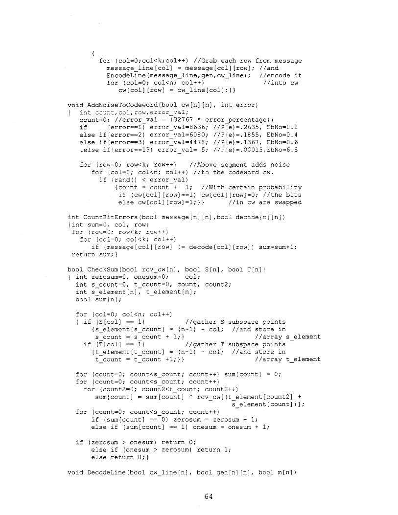
for (col=O;col<k;col++) //Grab each row from messagemessage_line[col] = message[col] [row]; //andEncodeLine(messageline,gen,cwline); //encode itfor (col=O; col<n; col++) //into cw
cw[col][row] = cwline[col];}}
void AddNoiseToCodeword(bool cw[n][n], int error)int count,col,row,error val;count=O; //errorval = (32767 * errorpercentage);if (error==i) errorval=8636; //P1e)=.2635, EbNo=0.2
else if(error==2) errorval=6080; //P(e)=.1855, EbNo=0.4else if(error==3) errorval=4478; //P(e)=.1367, EbNo=0.6...else if(error==19) errorval= 5; //Pe)=.03015,EbNo=6.5
for (row=O; row<k; row++) //Above segment adds noisefor (col=O; col<n; col++) //to the codeword cw.
if (rand() < errorval){count = count + 1; //With certain probability
if (cw[col] [row]==i) cw[col] [row]=O; //the bitselse cw[col][row]=1;}} //in cw are swapped
int CountBitErrors(bool message[n] [n],bool decode[_-] [n]){int sum=O, col, row;for (row='; row<k; row++)
for (col=O; col<k; col++)if (message[col] [row] != decode[col] [row!) sum=sum+l;
return sum;}
bool CheckSum(bool rcvcw[n], bool S[n], bool T'n]){ int zerosum=O, onesum=O; col;
int s count=O, tcount=O, count, count2;int selement[n], telement[n];bool sum[n];
for (col=O; col<n; col++){ if (S[col] == 1) //gather S subspace points
{s_element[scount] = (n-1) - col; //and store ins_count = s count + 1;} //array selement
if (T[col] == 1) //gather T subspace points{t_element[tcount] = (n-1) - col; //and store int_count = t count +1;}} //array telement
for (count=O; count<s count; count++) sum[count] = 0;for (count=O; count<scount; count++)
for (count2=0; count2<tcount; count2++)sum[count] = sum[count] A rcvcw[(telementFcount2] +
s_element~count])];for (count=O; count<scount; count++)
if (sum[count] == 0) zerosum = zerosum + 1;else if (sum[count] == 1) onesum = onesum + 1;
if (zerosum > onesum) return 0;else if (onesum > zerosum) return 1;else return 0;}
void DecodeLine(bool cw line[n], bool gen[n] [n], bool m[n])
64

rcvcw[n];int maj,col,row;
for (col=O; col<n; col++) //Creating copy of cwlinercvcw[col] = cw_line[col]; //in local variable.
{m[42]=CheckSum(rcvcw,v6v5v4v3,v2vl); //computem[43]=CheckSum(rcvcw,v6v5v4v2,v3vl); //value of
m[44]=CheckSum(rcv_cw, v67574vl, v3v2 ; //vector m4...m[56]=CheckSum(rcvcw,v4v3v2vl,v6v5);for (col=0; col<n; col++) //Calculate m4 times G4
{sum=0; //and subtact off of r.for (row=42; row<k; row++)sum = sum ^ (m[row]&&gen[col][row]);rcvcw[col] = rcvcw[col] ^ sum;}}
if (r>=3){m[22]=CheckSum(rcvcw,v6v5v4,v3v2vl); //compute m3...m[41]=CheckSum(rcvcw,v3v2vl,v6v5v4);for (col=0; col<n; col++) //Calculate m3 times G3
{sum=0; //and subtact off of r'.for (row=22; row<42; row++)sum = sum ^ (m[row]&&gen[col][row]);rcv cw[col] = rcv cw[col] ^ sum;}}
if (r>=2){m[7] =CheckSum(rcvcw,v6v5,v4v3v2vl); //Compute m2...m21]=CheckSum(rcv_cw,v2vl,v6v5v4v3);for (col=0; col<n; col++) //Calculate m2 times G2
{sum=0; //and subtact off of r''.
(r==4)
{sum=0
//For min//majority vote on r'
== 1) maj = maj + 1;=1; else m[0]=0;}}
if (r>=0){maj=0;
for (col=0; col<n; col++)if (rcv_cw[col]
if (maj > 32) m[0]
if
ml
we simply do a'''
void DecodeBlock(bool cw[n][n], bool gen[n][n], bool decode[n][n]){int col, row;bool decodeline[n];bool cw_line[n];
for (row=0; row<k; row++){for (col=0; col<n; col++) //Grab each row from
cw lineicol] = cw[col][row]; //kXn decoded rowsDecodeLine(cw_line,gen,decodeline);//and decode themfor (col=O; col<k; col++) //into a final block.
decode col][row] = decodeline[col];}}
//******************** MAIN PROGRAM *******************
int main(){int test;
int error, bit error count, frame error count;
65
for (row=7; row<22; row++)...}}if (r>=l)
{m[l] =CheckSum(rcvcw,v6,v5v4v3v2vl); //Compute...m[6] =CheckSum(rcv_cw,vl,v6v5v4v3v2);for (col=0; col<n; col++) //Calculate ml times Gl
//and subtact off of r'''.for (row=1; row<7; row++)...}}
{ bool sum;

long runningbit_errorcount;float BER,k2,running_error;
bool message[n][n]; //size nXn but only use kXk of itbool decode[n][n]; //decoded message (also kXk bits)bool cw[n][n]; //codewordbool gen[n][n]; //generator matrix
CreateGeneratorMatrix ,gen);for (error=1; error<20; error++){printf ("\nerror%d ",error);for (r=1; r<5; r++){if (r==1) k= 7; else if (r==2) k=22;else if (r==3) k=42; else if (r==4) k=57;runningbiterror count=O;frameerrorcount=0;for (test=0; test<1000; test++)//Runs 1000 test frames
{srand(test); // for each value of r// and prints results
CreateRandomMessage(message);EncodeMessage(message,gen,cw);AddNoiseToCodeword(cw,error);DecodeBlock(cw,gen,decode);bit errorcount=CountBitErrors(message,decode);
if (bit error-count != 0) frame error count += 1;running bit errorcount += biterrorcount;}printf ("%d ",frameerrorcount);printf ("%d ",running_biterrorcount);running_error = runningbiterror count;k2 k*k*10;BER = runningerror / k2;printf ("%.4f ",BER);} }
return 0;}
66

2b) Abbreviated C program for 2-D Soft code simulation:this code simulates iterative erasure decoding as specifiedin Appendix 1 sections f and g. When a procedure isidentical to one in Appendix 2b, it is specified as suchand thus not repeated.
void CreateGeneratorMatrix(bool gen[n][n]){...same as 2a
void CreateRandomMessage (bool message [n] [n]){...same as 2a}
void EncodeLine(bool message_line[n], ...)
{...same as 2a}
void EncodeMessage(bool message[n] [n], ...)
{ int col, row;bool message_line[n], cwline[n];
for (row=0; row<k; row++){...same as above}
for (col=0; col<n; col++){for (row=0; row<k; row++)
messageline[row] = cw[col][row]EncodeLine(messageline,gen,cw line
for (row=0; row<n; row++)CwLcol][row] = cw line[row];}}
void AddNoiseToCodeword (bool cw [n]
if (error==l) errorval =else if (error==2) errorval =else if (error==3) error val =...else if(error==18) error val =
[n],9326;
68955311
30;
//Grab each col from//kXn encoded rows
;//and encode//them into an//nXn block
//P(e)=.2846;; //P(e)=.2104;; //P(e)=.1621;
//P(e)=.0009;
if (error==1)else if (error==2)...else if(error==18)
errorval2 = 7972;
error val2 = 5328;
error val2 = 2;
//P(e)=.2433;//P(e)=. 1626;//P(e)=.0001;
for (row=0; row<n; row++)for (col=0; col<n; col++) //add noise to codeword{ number = rand();
if (cw[col][row]==1) corruptcw[col] [row]='1';else corruptcw[col][rowV='0';if (number < errorval){ corrupt cw[col][row]='X'; //bits are undecided.sumX+=1;}
if (number < errorval2) //bits are swapped{ if (cw[col][row]==1) corruptcw[col] [row]='0';
if (cw[col] [row]==0) corruptcw[col] [row]='l';sum+=1; } }
int CountBitErrors(bool message[n] [n],bool decode[n] [n]){...same as 2a}
bool CheckSum(bool rcvcw[n], bool{...same as 2a}
S[n], bool T[n])
67
;)

void DecodeLine(bool cwline[n], bool gen[n][n], bool m[n]){...same as 2a}
void ErasureDecodeLine(char eracwline[n], ...){int col, distance0=O, distancel=O;bool cwline[n],temp_decodelineO[n],tempdecodelinel[n];
for (col=0; col<n; col++) //replace Xs with Os{ //and hard decode
if (eracw_line[col]=='O') cw_line[col]=0;else if (eracw_line[col]=='l') cw_line[col]=l;else if (eracwline[col]=='X') cw_line[col]=0;}
DecodeLine(cw line, gen, temp_decodeline0);for (col=0; col<n; col++) //replace Xs with is{ //and hard decode
if (eracw_line[col]=='O') cw_line[col]=O;else if (eracw_line[col]=='l') cw_line[col]=l;else if (eracw_line[col]=='X') cw_line[col]=1;}
DecodeLine(cw line, gen, tempdecodelinel);for (col=0; col<n; col++) //determine Hamming distances{if ((eracw_line[coll=='O') &&
(tempdecode lineO[col]==1)) distanceC +=1;else if ((eracw line[col]=='i') &&
(temp_decodelineO[col]==O)) distanceO +=1;}for (col=O; col<n; col++) //Note that we consider
//distances from X to be zero for both cases.if ((era cw linefcol]=='O') &&
(tempdecodelinel[col]==l)) distancel +=l;else if ((eracw_line[col]=='1') &&
(tempdecode linel[col]==O)) distancel +=1;}
if (distanceO < distancel)for (col=0; col<n; col++)
decodeline[col] = tempdecodeline0[col];else
for (col=0; col<n; col++)decode line[col] = temp decode linel[col];}
void DecodeBlock(char corruptcw[n][n], ...){int col, row, count;bool decodeline[n], reencodeline[n], cwline[n];char eracw_line[n], vertcorrectgrid[n][n];char hori _correctgrid[n][n];
// We do this procedure 2ce. First we do iterations//impartial, then we do last iteration siding with hori.for (count=0; count<5; count++){for (col=0; col<n; col++)
{for (row=0; row<n; row++) //Grab each col***era cw line[row] = corruptcw[col][row];
ErasureDecodeLine(eracw_line,gen,decodeline);EncodeLine(decode line,gen,re encode line);for (row=0; row<n; row++){if (corruptcw[col][row]=='0')
{if (reencodeline[row]==0)vertcorrect_grid[col][row]='O';
else if (re encode line[row]==1)
68

vertcorrect_grid[col][row]='X';}else if (corruptcw[col][row]=='1'){ ... follow impartial rules}else if (corrupt_cw[col][row]=='X'){ ... follow impartial rules}}
for (row=O; row<n; row++){for (col=O; col<n; col++) //Grab each row***
... do the same as did for columns}for (col=O; col<n; col++)//Combine to make corrupt_cw
for (row=O; row<n; row++)//the overall correct grid{if (vertcorrect_grid[col][row]=='0')
{if (hori _correctgrid[col][row]=='0')corruptcw[col][row]='0';
else if (hori correctgrid[col][row]=='1')corruptcw[col][row]='X';
else if (hori _correctgrid[col][row]=='X')corrupt cw[col][row]='0';}
else if (vertcorrect_grid[col][rowj=='1'){...continue with impartial calculations}}}
for (count=O; count<1; count++){...repeat procedure above expect do the calculations
that involve sizing with the horizontal.}// Now we simply do the normal decode.for (col=O; col<n; col++){for (row=O; row<n; row++) //Grab each col
era cw_line[row] = corrupt_cw[col][row];ErasureDecodeLine(eracw_line,gen,decode line);for (row=O; row<k; row++)
decode[col][row] = decodeline[row];}for (row=O; row<k; row++){for (col=O; col<n; col++) //Grab each row
cw line[col] = decode[col][row];DecodeLine(cwline,gen,decodeline);for (col=O; col<k; col++)
decode[col][row] = decode line[col];}}
//********************* MAIN PROGRAM ******************
int main(){int test;int error, biterrorcount, frameerror count;long runningbiterrorcount;float BER,k2,running_error;bool message[n][n]; //size nXn but only use kXkbool decode[n][n]; //decoded message (also kXk bits)bool cw[n][n]; //codewordbool gen[n][n]; //generator matrixchar corruptcw[n][n];
CreateGeneratorMatrix(gen);for (error=1; error<19; error++)
{for (r=1; r<5; r++){if (r==1) k= 7; else if (r==2) k=22;else if (r==3) k=42; else if (r==4) k=57;runningbiterrorcount=O;frameerrorcount=0;for (test=O; test<1000; test++) //Runs 1000 frames{ srand(test);
69

CreateRandomMessage(message);EncodeMessage(message,gen,cw);AddNoiseToCodeword(cw,corruptcw,error);DecodeBlock(corrupt_cw,gen,decode);bit errorcount=CountBitErrors(message,decode);if (biterrorcount != 0) frameerror count += 1;running_bit_errorcount += biterrorcount;}
printf ("%d ",frameerrorcount);printf ("%d ",running_bit error count);running_error = runningbit error count;k2 = k*k*10;BER = runningerror / k2;printf ("%.4f",BER);}}
return 0;}
70

APPENDIX 3: PHASE II THROUGHPUT CALCULATION PROGRAM
This is the MATLAB script file that is used to
generate graphs for various throughputs and e values. Usingthe probabilities calculated in section 3, this filedetermines optimal packet sizes and throughputs of theadaptive code for various fading environments. This filealso calculates the throughput of the optimal non-adaptivecode.
al = zeros(1,120); %a = Pr(frame decodes incorrectly)a2 = [06.825 04.779 03.207 02.013 01.256 0.706 ... 0];a3 = [67.611 61.298 54.542 47.494 40.414 33.500 ... 0];a4 = [95.026 93.160 90.860 87.981 84.420 80.180 ... 0];a5 = [99.205 98.824 98.287 97.546 96.545 95.220 ... 0];
bl = 1 - (al / 100); %b = Pr(frame decodes correctly)
b2 = 1 - (a2 / 100); b3 = 1 - (a3 / 100);b4 = 1 - (a4 / 100); b5 = 1 - (a5 / 100);
x = (.25:.25:30); % x = x-axiskl = 7; k2 = 22; k3 = 42; k4 = 57; k5 = 64;
for m2 = 1:20m = .5 * m2;for s2 1:20
s = .25 * s2;for 1 = 1:500c = bl .^ 1; %c=Pr(l frame block decodes correctly)y = (1/(((2*pi)^.5)*s)) * exp(-1 * (x-m).A2 /
(2*s^2)); % y = Norm(m,s) curvet = c*((kl*l)-64)/(64*l); % t = throughputt(t<0) = - t(t<0)*0; % set neg thrpts to 0tnorm = t .* y; % normalize throughputstnorml(l) = .25 * (t * y'); % overall thpts in tnormlend[thruputl(m2,s2),thruputll(m2,s2)] = max(tnorml);% store best thrpt in thruput & best 1 in thruputl
endend
for m2 = 1:20m = .5 * m2;for s2 = 1:20
s = .25 * s2;for 1 = 1:500
{... repeat above expect c = b2 .^ 1 and store inthruput2(m2,s2) }
endend
{... repeat again for b3 and b4}
71

for m2 = 1:20for s2 = 1:20
d = [thruputl(m2,s2) thruput2(m2,s2) thruput3(m2,s2)thruput4 (m2,s2) thruput5(m2,s2)];
[thruputx(m2,s2),thruputx2(m2,s2)] = max(d);end %This segment picks the best
end %non-adaptive code for a given m & s.
for m2 = 1:20m = .5 * m2;for s2 = 1:20
s = .25 * s2;for 1 = 1:500cl = bl .^ 1; %c=Pr(l frame block decodes correctly)
tl = c1*((kl*l)-64)/(64*l); % t = throughputc2 = b2 .^ 1;t2 = c2*((k2*l) -64)/(64*l);c3 = b3 .^ 1;t3 = c3*((k3*l)-64)/(64*l);c4 = b4 .^ 1;t4 = c4*((k4*l)-64)/(64*l);c5 = b5 .^ 1;t_5 = c5*((k5*1)-64)/(64*1);-or e = 1:120
t(e) max([tl(e) t2(e) t3(e) t4(e) t5(e)]);end;
(t<0) = - t(t<0)*O; %set any negative thrpts t
y = (1/(((2*pi)A.5)*s)) * exp(-1 * (x-m).^2 /(2*sA2)); % y = Norm(m,s) curv
tnorm = t .* y; % normalize throug
tnorml(l) .25 * (t * y'); % store overall thend(thruputa(m2,s2),thruputal(m2,s2)] = max(tnorml);estore best throughput in thruput & best 1 in thruputl
endend
hputsrpts
%mesh (thruputa-thruputx);%mesh(thruputa ./ thruputx);
%adaptive - non-adaptive%adaptive / non-adaptive
subplot (2,1,1);mesh(thruputx); %thruputs for best non-adaptive codesubplot (2,1,2);mesh(thruputx2); %the specific code used
%subplot(2,1,1);%mesh(thruputa); %thruputs for adaptive code
%subplot (2,1,2);%mesh(thruputal); %value of 1 at those thruputs
%subplot(2,2,1); %we can also get thruputs and 1 values%mesh(thruputl); %for individual codes.%subplot(2,2,2);%mesh(thruput2);% ... mesh(thruput4);
72
o 0
e

APPENDIX 4: MARKOV CHAIN MODEL AND ITS AUTO-CORRELATION
This MATLAB script file runs the Markov Chain model offading. It also calculates the auto-correlation of thestate of the chain as a function of iterations. Thisfunction is used to determine how many iterations equal 1second of time.
m = 5; % range from 0 to 10 in steps of 0.5s = 2; % range from 0 to 5 in steps of 0.25lambda = zeros(1,80);mu = zeros(1,80);sumstate = zeros(1,80);
rand('seed',O); % set -and # seed to startup valuex = (.25:.25:20); % x = u-axis (index for Eb/Nos)y = (1/(((2*pi)A.5)*s)) * exp(-1 * (x-m).^2 / (2*sA2));
% y = Norm(m,s) curvestate = m*4; % state = y's index corresponding to mlambda(state) = .05;while ( (lambda(state)>=0)&(mu(state)>=0)&(state<80)mu(state+1) = lambda(state)*y(state)/y(state+l);lambda(state+1) = .1 - mu(state+1);state = state+l; % setting up lambda and mu vectors
endlambda(state)=0; mu(state)=.1;state = m*4;lambda(state) = 2*lambda(state); % readjust lambda and mu atmu(state) = 2*mu(state); % mean value
for t = 1:100000 %-----------Creates Fading--------------------------if (state==(m*4)) % m*4 b/c x in .25 increments
if (rand > 0.5) dirgauss = 1;else dirgauss = 0; end;
end;staterand = rand;if (staterand < lambda(state)) state=state+1;elseif (staterand < (lambda(state)+mu(state))) state=state-1; end;
if (dirgauss==1)statex(t) = .25 * state;
else stref = (m*8)-state; % reflect state to other side of chainstatex(t) = .25 * st ref; end;
end;save mclOOk
AmtTau = 10000; % How far do we calculate Rt?Amt t = 90000; % How many points do be average out?for tau = 1:AmtTau %------Calculates coorlelation--------
SumR = 0;for t = 1:Amt_t
SumR = SumR + (statex(t+tau)-m)*(statex(t)-m);end;R(tau) = SumR / Amt t;
73

end;save mc90k;subplot (2, 1, 1) ; plot (R);%plot (x, y);subplot(2,1,2); plot(statex);%subplot(2,1,2); %plot(x,sumstate);
74

APPENDIX 5: PHASE II THROUGHPUT SIMULATION PROGRAM
This script file is used to simulate the throughputperformance of the ARQ/AFEC system. The UsingCtrlPktsvariable is set appropriately to simulate the desiredprotocol.
clear;%variables to inputm = 5;s = 2.0;1 = 18;delay = 0;iterations = 1000000;UsingCtrlPkts = 1;pkts_per_iter = 5;
% clear all variables
% mean of gaussian fade% standard deviation of gaussian fade% length of block
% # of packets to transmit% 1=ctrl pkts, 0=code field in header% 500 for 1 GHz, 5 for 10 MHz
for trials = 1:5
delay = 25 * (trials-1);%delay = 100 * trials + 100;%delay = 500 * trials + 500;
rand('seed',0);if (UsingCtrlPkts==0)
overhead = 72;else overhead = 64; end;
al = zeros(1,80);a2 = [06.825 04.779 03.207 ...a3 = [67.611 61.298 54.542 ...a4 = [95.026 93.160 90.860 ...aS = [99.205 98.824 98.287 ...bl = 1 - (al / 100);b2 = 1 - (a2 / 100);...b5 = 1 - (a5 / 100);cl = bl .^ 1; c2 = b2 .^ 1;...c5 = b5 . 1;
x = (.25:.25:20); % x
k1 = 7; k2 = 22; % #k3 = 42; k4 = 57; % kk5 = 64;
% delays 0 25 50 75 100% delays 200 300 400 500% delays 1k 1.5k 2k 2.5k 3k 3.5k 4k
% set rand # seed to startup value
% # of bits for CRC, pkt #, control%using 64 again to compare to%NoDelay... will change to 72
% a = Pr(frame decodes incorrectly)0];0];01;01;% b = Pr(frame decodes correctly)
% c = Pr(block decodes correctly)
= x-axis (index for Eb/Nos)
info bits per line of block*1 - overhead = # info bits per block
n = 64;ratel = ((k1*l)-overhead)/(n*l);rate2 = ((k2*l)-overhead)/(n*l);..rate5 = ((k5*l)-overhead)/(n*l);
% create vectors that store which codefor c = 1:80 % gives max throughput & value for that Pr
[maxPrC(c),maxCode(c)] =max([cl(c)*ratel c2(c)*rate2...c5(c)*rate5]);end;
actualEbNo =m;
assumedEbNo =m;
% determines noise to pick Pr(success) from% determines code transmitted & received
75

transl = 0; trans2 = 0; % # of times transmitter switches codetrans3 = 0; trans4 = 0; % while system using code xtrans5 = 0;numcodel = 0; numcode2 = 0; % running sum of the number ofnumcode3 = 0; numcode4 = 0; % times that code x is transmittednumcode5 = 0;sum-success = 0; % running sum of # of correct decodes
for d = 1:10000Delay(d)=m;
% initialize delay matrix to the% mean EbNo value.
end;assumedPtr = 1; % initialize delay pointersactualPtr = assumedPtr + delay;
% Setting up variables for Markov Chainlambda = zeros(1,80); % lambda & mu used for Markov Chain.mu = zeros(1,80); % sumstate used to check chainsumstate = zeros(1,80); % distribution (make sure Gaussian)
y = (1/(((2*pi)^.5)*s)) * exp(-1 * (x-m).^2 / (2*sA2));% y = Norm(m,s) curve
state = m*4; % state = y's index corresponding to mlambda(state) = .05;while ( (lambda(state)>=0)&(mu(state)>=0)&(state<80)mu(state+1) = lambda(state)*y(state)/y(state+l);lambda(state+1) = .1 - mu(state+1);state = state+1; % setting up lambda and mu vectors
endlambda(state)=0; mu(state)=.1;% terminate positive end properlystate = m*4;lambda(state) = 2*lambda(state); % readjust lambda and mu at meanmu(state) = 2*mu(state); % value (b/c counted 2ce, 1 pos, 1 neg)
t = 0;while (t < iterations)
t = t + 1;
%------------Gaussian Procedure: uses and updates-------------------%------------variable state to update variable -------------------
%------------actualEbNoif (state==(m*4))
if (rand > 0.5) dirgauss = 1;else dirgauss = 0; end;
end;
% When state at mean, it has a% 50/50 chance of going positive/% normal or going negative/% reflection of positive
staterand = rand; % Calculate next normal stateif (staterand < lambda(state)) state=state+1;elseif (staterand < (lambda(state)+mu(state))) state=state-1; end;
if (dirgauss==l)sumstate(state) = sumstate(state)+1; % State positiveactualEbNo = state;
elsestref = (m*8)-state; % reflect state to other side of chainif (stref>0)sumstate(stref) = sumstate(stref)+1;actualEbNo = st ref;
else
76

actualEbNo = 0;end;
end;
% when state < 0, modem unlock and% Pr(success) = 0;
%--------Delay procedure for picking code that system -------------%--------thinks is current -------------
Delay(actualPtr) = actualEbNo; % use variable assumedEbNo2assumedEbNo2 = Delay(assumedPtr); % to compute transitionsactualPtr = actualPtr + 1; % info for throughputif (actual Ptr==10001) actualPtr = 1; end;assumed Ptr = assumedPtr + 1;if (assumedPtr==10001) assumedPtr = 1; end;if (assumedEbNo2==0) assumedEbNo2=1; end; %send at least codel
%--------Collect the variables that are needed to -----------------%--------calculate the throughput -----------------
if (actualEbNo==0)success = 0;
elseif (maxCode(assumedEbNo2) -= maxCode(assumedEbNo))
if (UsingCtrlPkts==l)%tracks # times code changed while system in code xif (maxCode(assumedEbNo)==) transl=transl+1;elseif (maxCode(assumedEbNo)==2) trans2=trans2+1;...elseif (maxCode(assumedEbNo)==5) trans5=trans5+l; end;
end;assumedEbNo = assumedEbNo2; % start using assumedEbNo now
end
if (maxCode(assumedEbNo)==l)PrSucc=cl(actualEbNo); % calculate correct probabilitynum codel=num codel+1; % of success and calculate running
elseif (maxCode(assumedEbNo)==2) % sum of # of times each codePrSucc=c2(actualEbNo); % is transmittednum code2=numcode2+1;
...elseif (maxCode(assumedEbNo)==5)PrSucc=c5(actualEbNo);numcode5=numcode5+1;
end;if (PrSucc > rand) success=l;else success=0; end;
end;
if (success) % sum of the number ofsumsuccess = sumsuccess + 1; % successful decodes
end;
end;
% -------------------------------------------% Now we calculate throughput. For system using ctrl info in packets,% increase overhead and zeroize transitions information. For system% using control packets, subtract transitions info because these use% control pkts and are not counted in throughput.% -------------------------------------------
PrCorrect = sum-success / iterations;
77

numcodel = numcodel * pkts_per_iter;numcode2 = numcode2 * pktsper_iter;...numcode3 = numcode5 * pkts_per_iter;numcode t = numcodel + num code2 + ... +
%Mult by pkts_per_iter and%thus each numcode actually% represents x amt of pkts.
num code5;
%# of info bits txmtd by each code in the session% ...divide sum by the total # of bits txmtd in the sessionRatel = (numcodel-transl)*((kl*l) - overhead);Rate2 = (numcode2-trans2)*((k2*l) - overhead);...Rate5 = (num code5-trans5)*((k5*l) - overhead);OverallRate = (Ratel+Rate2+Rate3+Rate4+Rate5) / (n*l*numcode t);
Throughput = PrCorrect * OverallRate % Thrput for Selective Repeat
end;
%subplot (2,1,1);%plot (y);%subplot(2,1,2);%plot(sumstate);
78

REFERENCES:
[1] Buch, Gabriele; Burkert, Frank, "Concatenated Reed-Muller Codes
for Unequal Protection," IEEE Communications Letters, vol. 3, no.7, July 1999.
[2] Chang, Yuwei, "A New Adaptive Hybrid ARQ Scheme," IEEE
Transactions on Communications, vol. 43, no. 7, July 1995.
[3] Efficient Channel Coding, Inc. "Technical Description of TurboProduct Codes." Eastlake, OH, Version 3.1, June 1998.
[4] Evans, John, "New Satellites for Personnal Communications,"Scientific American, pp 71-77, April 1998.
[5] Forney, David, Class Notes for 6.451: Principles of Digital
Communications. MIT Spring 2000.
[6] Howald, Rob, "Symbol Error Expressions Demystified,"
Communication Systems Design, vol. 6, no. 2, Feb 2000.
[7] Kallel, Samir, "Efficient Hybrid ARQ Protocols with Adaptive
Forward Error Correction," IEEE Transactions on Communications,
vol. 42, no. 2/3/4, Feb/Mar/Apr 1994.
[8] Lin, Shu; Costello, Daniel; Miller, Michael, "Automatic-Repeat-
Request Error Control Schemes," IEEE Communications Magazine,vol.22 no.12, pp 5-17, Dec. 1984.
[9] Pyndiah, Ramesh, "Near-Optimal Decoding of Product Codes: Block
Turbo Codes," IEEE Transactions on Communications, vol.46 no.8,
pp 1003-1010, Aug. 1998.
[10] Shiozaki, Akira, "Adaptive Type-II Hybrid Broadcast ARQ System,"
IEEE Transactions on Communications, vol. 44, no. 4, April 1996.
[11] Shiozaki, Akira; Okuno, Kiyoshi; Suzuki, Katsufumi; Segawa,Tetsuro, "A Hybrid ARQ Scheme with Adaptive Forward Error
Correction for Satellite Communications," IEEE Transactions on
Communications, vol. 39, no. 4, April 1991.
[12] Wicker, Stephen B, Error Control Systems for DigitalCommunication and Storage. New Jersey, Prentice Hall, 1995.
79