Design of Experimentmethodology

ANOVA、 FFD、CCD、Mixture Design

Response surface design

Kung, Chun-Haokch800721@gmail.comChemical engineering department in NCKU

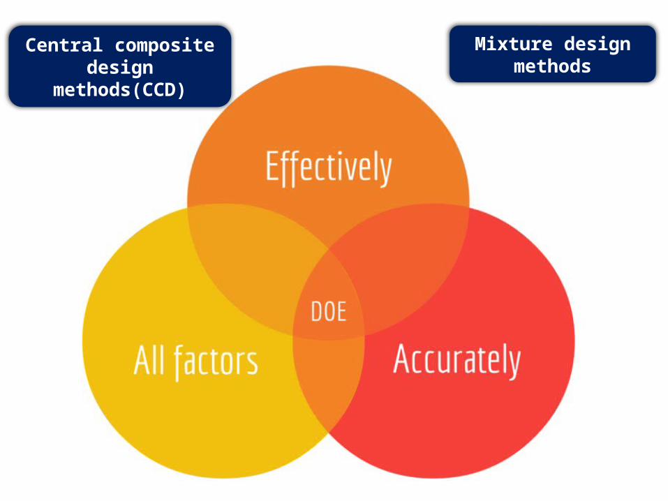
Central composite design methods(CCD)

Mixture design methods

Know situation

Design of experiment

Optimized process

Flow chart

Response surface design

• Help you better understand and optimize your response.

• Used to refine models after you have determined important factors using factorial designs

Advantages of Response surface design

Factorial Points : Estimated main factor & interaction

Axial Points : Estimated pure quadratic form

Center Points : Estimated pure Error

→ Building a quadratic response surface→ Resolves both main effects and interactions

Central composite design (CCD)

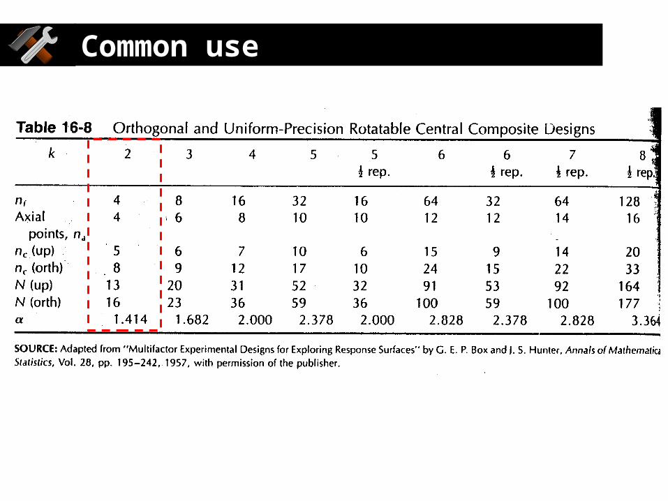
Common use

8

Level  Temperature () Annealing time (mins)120    5.0

1 115    6.50 100 10.0-1 85  13.5- 80  15.0

Run Temp. Time Temp. Time

1 -1 -1 85 13.5

2 -1 1 85 6.5

3 1 -1 115 13.5

4 1 1 115 6.5

5 0 0 100 10

6 0 0 100 10

7 0 0 100 10

8 0 - 100 15

9 0 100 5

10 - 0 80 10

11 0 120 10

Design matrix

Reference: Michael Grätzel, Advanced Functional Materials, 24, 3250(2014)

Effect of Annealing Temperature on Film Morphology of Organic–Inorganic Hybrid Pervoskite Solid-State Solar Cells

120

5 mins

15 mins

8100

80

run Temp. Time Voc (V) Jsc (mA/cm2) FF PCE (%)

1 80 10 0.77 7.07 0.72 3.89

2 85 13.5 0.72 10.30 0.59 4.44

3 85 6.5 0.25 12.98 0.37 1.23

4 100 15 0.78 13.86 0.72 7.77

5 100 10 0.78 11.99 0.73 6.78

6 100 5 0.81 6.63 0.73 3.92

7 115 13.5 0.71 12.80 0.66 5.99

8 115 6.5 0.72 13.18 0.71 6.72

9 120 10 0.71 11.42 0.68 5.50

Origin data-CCD

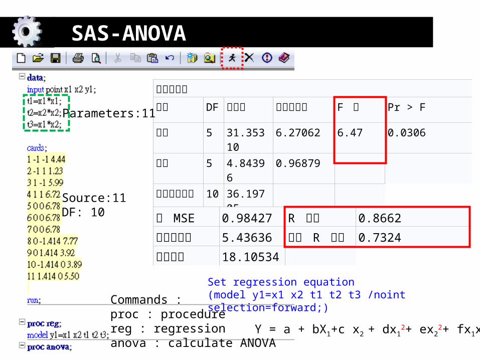
SAS-ANOVA

Source:11DF: 10

變異數分析來源 DF 和平方 平均值平方 F 值 Pr > F

模型 5 31.35310

6.27062 6.47 0.0306

誤差 5 4.84396

0.96879    

已校正的總計

10 36.19705

   

根 MSE 0.98427 R 平方 0.8662

應變平均值 5.43636 調整 R 平方

0.7324

變異係數 18.10534  Set regression equation(model y1=x1 x2 t1 t2 t3 /noint selection=forward;)Commands :

proc : procedurereg : regressionanova : calculate ANOVA

Y = a + bX1+c x2 + dx12+ ex2

2+ fx1x2

Parameters:11

參數估計值

變數 DF 參數估計

標準誤差

t  值 Pr > |t|

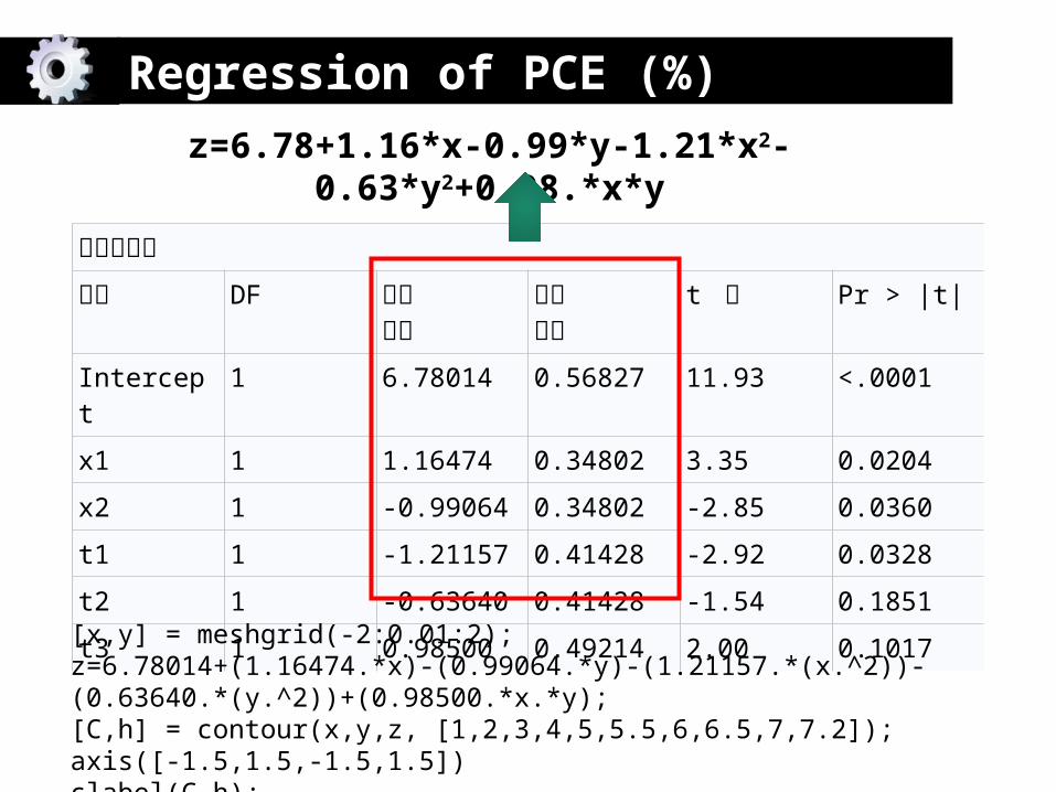
Intercept 1 6.78014 0.56827 11.93 <.0001

x1 1 1.16474 0.34802 3.35 0.0204

x2 1 -0.99064 0.34802 -2.85 0.0360

t1 1 -1.21157 0.41428 -2.92 0.0328

t2 1 -0.63640 0.41428 -1.54 0.1851

t3 1 0.98500 0.49214 2.00 0.1017

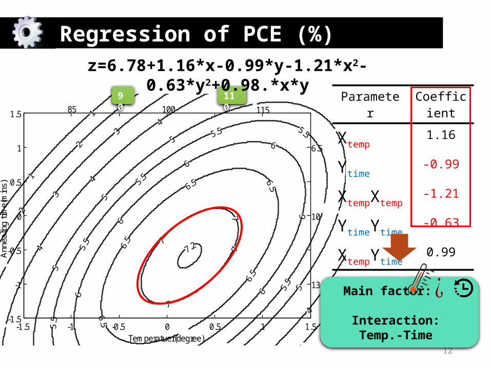
z=6.78+1.16*x-0.99*y-1.21*x2-0.63*y2+0.98.*x*y

Regression of PCE (%)

[x,y] = meshgrid(-2:0.01:2);z=6.78014+(1.16474.*x)-(0.99064.*y)-(1.21157.*(x.^2))-(0.63640.*(y.^2))+(0.98500.*x.*y);[C,h] = contour(x,y,z, [1,2,3,4,5,5.5,6,6.5,7,7.2]);axis([-1.5,1.5,-1.5,1.5])clabel(C,h);

12

Temperatuer(degree)

Ann

ealin

g tim

e(m

ins)

85 100 115

6.5

10

13.5

-1.5 -1 -0.5 0 0.5 1 1.5-1.5

-1

-0.5

0

0.5

1

1.5

Parameter Coefficient

Xtemp1.16

Ytime-0.99

XtempXtemp-1.21

YtimeYtime-0.63

XtempYtime0.99

Main factor: Interaction: Temp.-Time

90

110

z=6.78+1.16*x-0.99*y-1.21*x2-0.63*y2+0.98.*x*y

¿

Regression of PCE (%)

Mixture design method

Cl

BrI

14

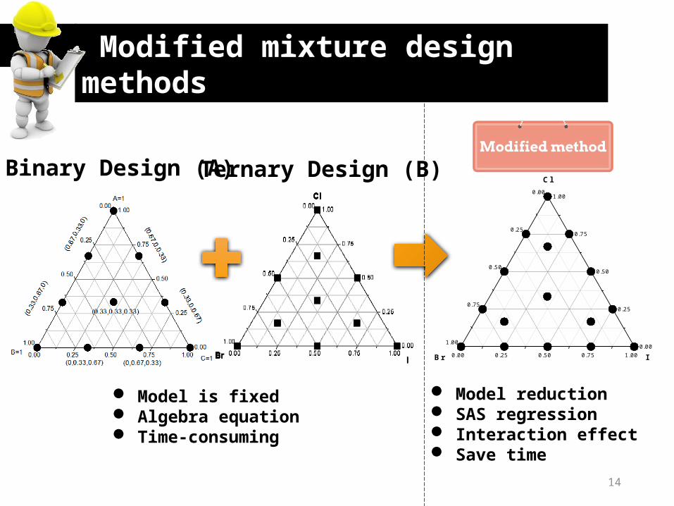
Model is fixed Algebra equation Time-consuming

Model reduction SAS regression Interaction effect Save time

0.00 0.25 0.50 0.75 1.00

0.00

0.25

0.50

0.75

1.000.00

0.25

0.50

0.75

1.00

IBr

ClBinary Design (A) Ternary Design (B)

Modified mixture design methods

Advantages of mixture design

• Designs for these experiments are useful because many product design and development activities in industrial situations involve formulations or mixtures.

16

Statics and regression examples

17

Mixture design methodology

RegressionExperimental data Contour plot1. 2. 3.

SAS 9.3 MATLAB R2013a

0.00 0.25 0.50 0.75 1.00

0.00

0.25

0.50

0.75

1.000.00

0.25

0.50

0.75

1.00

IBr

Cl

Origin data

Ratio MACl MABr MAI Voc(V) Jsc (mA/cm2) FF (%) PCE (%)

1 1 0 0 0.76 10.31 69% 5.422 0 1 0 0.97 5.54 71% 3.813 0 0 1 0.78 9.76 70% 5.384 0.33 0.333 0.333 0.86 11.54 66% 6.545 0.5 0.5 0 0.97 4.76 70% 3.236 0 0.5 0.5 0.92 5.97 66% 3.587 0.5 0 0.5 0.71 12.10 72% 6.128 0.67 0.17 0.17 0.73 12.37 71% 6.389 0.17 0.67 0.17 0.97 10.66 64% 6.54

10 0.17 0.17 0.67 0.85 11.46 77% 7.5111 0.75 0.25 0 0.90 7.43 64% 4.3212 0.25 0.75 0 0.96 7.68 57% 4.1513 0.25 0 0.75 0.78 13.06 68% 6.8914 0.75 0 0.25 0.80 9.93 72% 5.6815 0 0.75 0.25 0.99 10.81 72% 7.7116 0 0.25 0.75 0.82 10.05 73% 6.01

Forward selection

SAS Regression

run;

proc reg;model y1=t1 t2 t3 t4 t5 t6 t7 t8 t9 t10 t11 t12 t13 /noint selection=forward;proc anova;

前進選擇 : 步驟 1 R 平方 = 0.6006 和 C(p) = 57.8286

前進選擇 : 步驟 2R 平方 = 0.8367 和 C(p) = 17.3612

前進選擇 : 步驟 7 R 平方 = 0.9792 和 C(p) = 1.7387

Click run

Model reduction

Parameter Coefficient

X1 t1

X2 t2

X3 t3

X1X2 t4

X1X3 t5

X2X3 t6

X1X2X3 t7

X1X2(X1-X2) t8

X1X3(X1-X3) t9

X2X3(X2-X3) t10

X1X1X2X3 t11

X1X2X2X3 t12

X1X2X3X3 t13

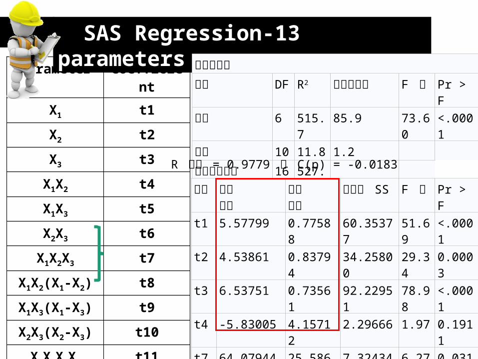
SAS Regression-13 parameters

變異數分析來源 DF R2 平均值平方 F 值 Pr > F

模型 6 515.7

85.9 73.60

<.0001

誤差 10 11.8 1.2    

未校正的總計 16 527.4

   

變數

參數估計

標準誤差

第二型 SS

F 值 Pr > F

t1 5.57799 0.77588 60.35377

51.69

<.0001

t2 4.53861 0.83794 34.25800

29.34

0.0003

t3 6.53751 0.73561 92.22951

78.98

<.0001

t4 -5.83005 4.15712 2.29666 1.97 0.1911

t7 64.07944 25.58609

7.32434 6.27 0.0312

t10 11.75880 7.90392 2.58452 2.21 0.1677

R 平方 = 0.9779 和 C(p) = -0.0183

Parameter Coefficient

X1 t1

X2 t2

X3 t3

X1X2 t4

X1X3 t5

X2X3 t6

X1X2X3 t7

X1X1X2X3 t11

X1X2X2X3 t12

X1X2X3X3 t13

SAS Regression-10 parameters

變異數分析來源 DF 和

平方平均值平方

F 值 Pr > F

模型 6 513.8

85.6 63.28

<.0001

誤差 10 13.53

1.35    

未校正的總計 16 527.4

 

變數

參數估計

標準誤差

第二型 SS

F 值 Pr > F

t1 5.26373 1.01318 36.52686

26.99

0.0004

t2 5.09614 0.83751 50.10738

37.03

0.0001

t3 5.81178 0.83751 65.16845

48.15

<.0001

t4 -6.08694

4.54785 2.42432 1.79 0.2104

t5 3.33659 4.54785 0.72845 0.54 0.4800

t7 59.03570

29.04160

5.59231 4.13 0.0695

R 平方 = 0.9743 和 C(p) = 2.7857

0

0.25

0.5

0.75

1 0

0.25

0.5

0.75

1

Cl

Br I0 0.1 0.2 0.3 0.4 0.5 0.6 0.7 0.8 0.9 1

0

0.1

0.2

0.3

0.4

0.5

0.6

0.7

0.8

0.9

1

7.4

7.2

7

6.5

6

5

6 6.5

7

5

6.5

6

0

0.25

0.5

0.75

1 0

0.25

0.5

0.75

1

Cl

Br I0 0.1 0.2 0.3 0.4 0.5 0.6 0.7 0.8 0.9 1

0

0.1

0.2

0.3

0.4

0.5

0.6

0.7

0.8

0.9

1

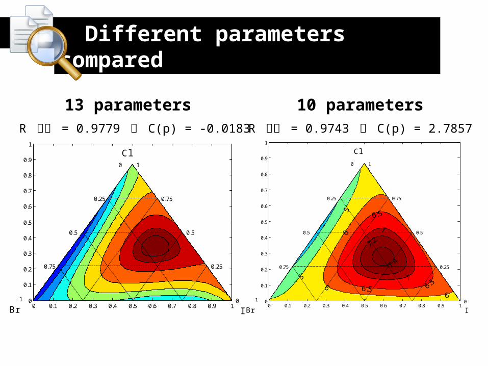
R 平方 = 0.9779 和 C(p) = -0.0183 R 平方 = 0.9743 和 C(p) = 2.7857

Different parameters compared

13 parameters 10 parameters

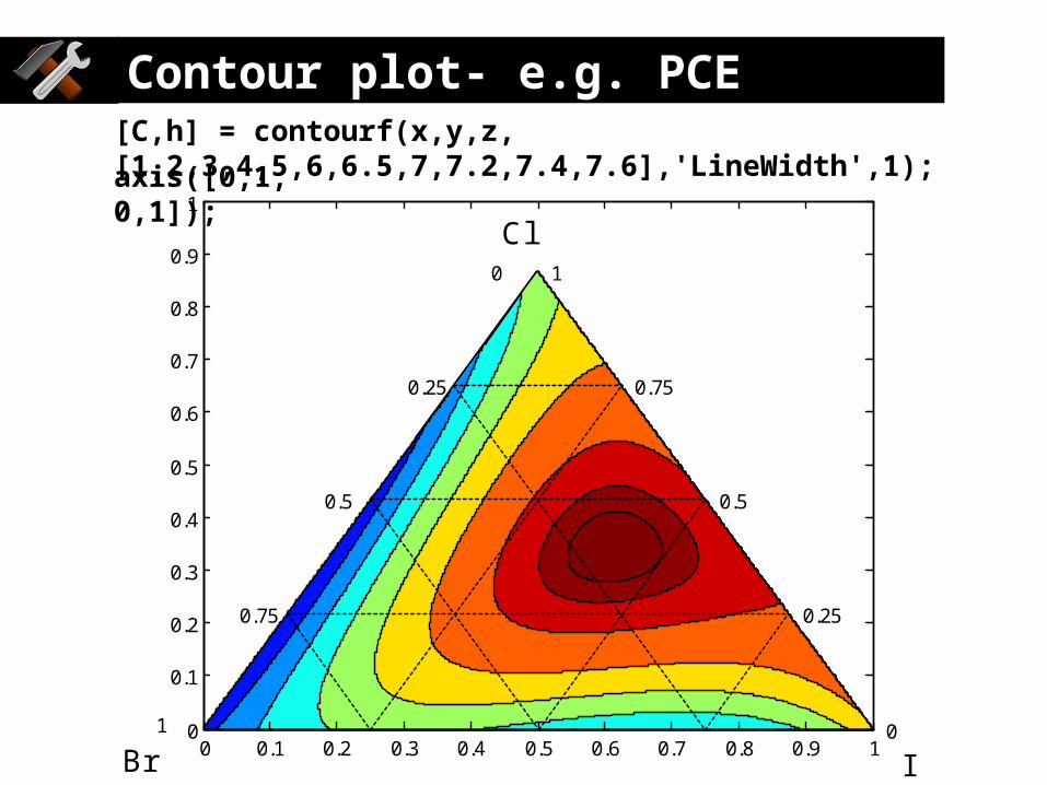
Contour plot- e.g. PCEA=tril(meshgrid(0:0.001:1));B=tril(meshgrid(1:-0.001:0)');C=tril(1-A-B);x=tril(0.5.*(1+C-B));y=tril((3^0.5)*0.5.*A);

z=5.57799.*A +4.53861.*B+6.53751.*C -5.83005.*A.*B +64.07944.*A.*B.*C+11.75880.*B.*C.*(B-C);

[C,h] = contourf(x,y,z, [1,2,3,4,5,6,6.5,7,7.2,7.4,7.6],'LineWidth',1);

axis([0,1,0,1]);

clabel(C,h,'manual','fontsize',15);hold onplot([0.375,0.625],[0.6495,0.6495],'k:');hold onplot([0.25,0.75],[0.433,0.433],'k:');hold onplot([0.375,0.75],[0.6495,0],'k:');hold onplot([0.25,0.5],[0.433,0],'k:');hold onplot([0.125,0.25],[0.2165,0],'k:');hold onplot([0.125,0.875],[0.2165,0.2165],'k:');hold onplot([0.25,0.625],[0,0.6495],'k:');hold onplot([0.50,0.75],[0,0.433],'k:');hold onplot([0.75,0.875],[0,0.2165],'k:');

先建立矩陣數列，從 0~1，間格0.001

利用 SAS迴歸得到的 Eq.

A=tril(meshgrid(0:0.001:1)) B=tril(meshgrid(1:-0.001:0)');

x=tril(0.5.*(1+C-B)); y=tril((3^0.5)*0.5.*A);

C=tril(1-A-B);

z=5.58.*A +4.54.*B+6.54.*C -5.83.*A.*B+64.08.*A.*B.*C+11.76.*B.*C.*(B-C);

e.g. 0.5*(1+0.001-0.998) e.g. *0.5*0.001

Function

0

0.25

0.5

0.75

1 0

0.25

0.5

0.75

1

Cl

Br I0 0.1 0.2 0.3 0.4 0.5 0.6 0.7 0.8 0.9 1

0

0.1

0.2

0.3

0.4

0.5

0.6

0.7

0.8

0.9

1

Contour plot- e.g. PCE[C,h] = contourf(x,y,z, [1,2,3,4,5,6,6.5,7,7.2,7.4,7.6],'LineWidth',1);

axis([0,1,0,1]);

78 10

9

11

12 12.5

12.7

1211

108

1110

0

0.25

0.5

0.75

1 0

0.25

0.5

0.75

1

Cl

Br I0 0.2 0.4 0.6 0.8 1

0

0.1

0.2

0.3

0.4

0.5

0.6

0.7

0.8

0.9

1

5

6

7

8

9

10

11

12

1

0.98

0.94

0.9

0.85

0.8

0.75

0.85

0.8

0

0.25

0.5

0.75

1 0

0.25

0.5

0.75

1

Cl

Br I0 0.2 0.4 0.6 0.8 1

0

0.1

0.2

0.3

0.4

0.5

0.6

0.7

0.8

0.9

1

0.7

0.75

0.8

0.85

0.9

0.95

1

0.6

0.65

0.68 0.7

0.75

0.8

0.850.9

0.55

0.7

0.7

0

0.25

0.5

0.75

1 0

0.25

0.5

0.75

1

Cl

Br I0 0.2 0.4 0.6 0.8 1

0

0.1

0.2

0.3

0.4

0.5

0.6

0.7

0.8

0.9

1

0.55

0.6

0.65

0.7

0.75

0.8

0.85

0.6

0.6

0.65

0.65 0.68

0.68

0.7

0.75

0.80.85

0.9

0.75

0.7

0.55

0

0.25

0.5

0.75

1 0

0.25

0.5

0.75

1

IBr

Cl

5 6 6.5 7 7.2

7.27

6.5

6

5

6

6.5

0 0.2 0.4 0.6 0.8 10

0.1

0.2

0.3

0.4

0.5

0.6

0.7

0.8

0.9

1

1

2

3

4

5

6

7

JscVoc FF PCE

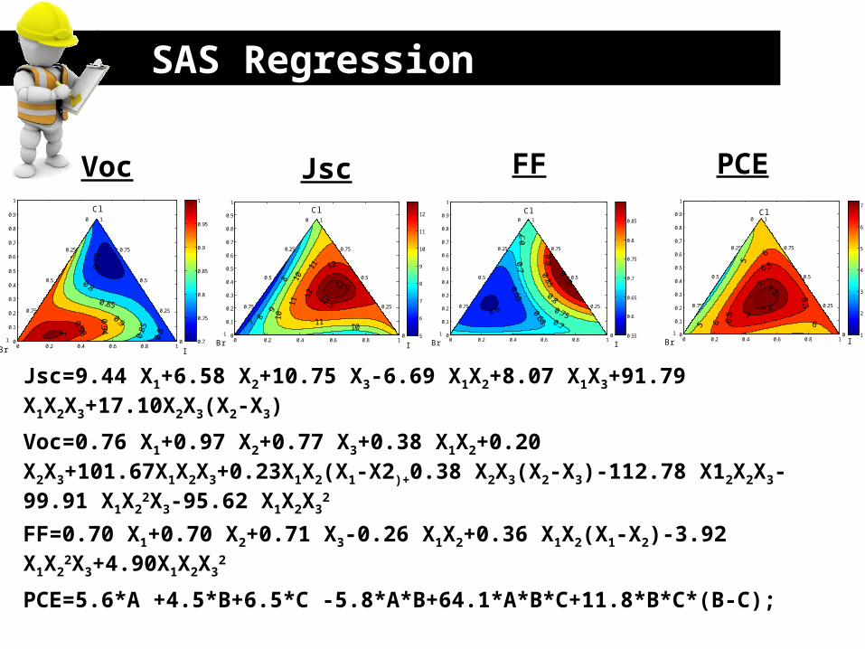
PCE=5.6*A +4.5*B+6.5*C -5.8*A*B+64.1*A*B*C+11.8*B*C*(B-C);

SAS Regression

Jsc=9.44 X1+6.58 X2+10.75 X3-6.69 X1X2+8.07 X1X3+91.79 X1X2X3+17.10X2X3(X2-X3)

Voc=0.76 X1+0.97 X2+0.77 X3+0.38 X1X2+0.20 X2X3+101.67X1X2X3+0.23X1X2(X1-X2)+0.38 X2X3(X2-X3)-112.78 X12X2X3-99.91 X1X2

2X3-95.62 X1X2X32

FF=0.70 X1+0.70 X2+0.71 X3-0.26 X1X2+0.36 X1X2(X1-X2)-3.92 X1X22X3+4.90X1X2X3

2

27

0

0.25

0.5

0.75

1 0

0.25

0.5

0.75

1

I

0 0.25 0.5 0.75 1 0.0 0.2 0.4 0.6 0.8 1.0-16

-14

-12

-10

-8

-6

-4

-2

0

MAPbCl0.30

Br0.15

I0.55

MAPbCl0.30

Br0.35

I0.30

MAPbCl0.30

Br0.55

I0.15

Curr

ent den

sity

(m

A/c

m2)

Voltage (V)

PCE Contour plotrun Cl Br I Voc Jsc FF PCE

 0.30 0.55 0.15  0.97 9.94 0.70 6.77

0.30 0.35  0.35  0.92 14.07 0.73 9.47

0.30 0.15 0.55 0.75 12.67 0.68 6.52

Cl

IBr

Verification by J-V curve

28

FFD(Full Factorial Design )

Factors and levels for the 23 Full Factorial Design

factorslevels

+ -A, P3HT:PCBM concentration 

(wt%) 2.5 1.5

B, rpm 600 1000

C, time (s) 60 40

Full Factorial Design

1.5wt% 600rpm 40s 600rpm 60s 1000rpm 40s 1000rpm 60sVOC (V) 0.04 0.60 0.70 0.72

JSC (mA/cm2) 2.94 7.22 1.21 1.03FF 0.29 0.32 0.32 0.30

PCE (%) 0.03 2.83 0.27 0.22

R.P (Ω ･ cm2)104 0.00083 278.8 71.68 99.72

R.S (Ω ･ cm2) 1.88 2.23 7.36 1.15

Run A B C Voc (V) Jsc (mA/cm2) FF PCE (%)

1 - + - 0.04 2.94 0.29 0.03

2 - + + 0.60 7.22 0.65 2.83

3 - - - 0.70 1.21 0.32 0.27

4 - - + 0.72 1.03 0.30 0.22

factors + -A, concentration  (wt%) 2.5 1.5B, revolution (rpm) 600 1000C , time (s) 60 40

2.5wt% 600rpm 40s 600rpm 60s 1000rpm 40s 1000rpm 60sVOC (V) 0.60 0.58 0.60 0.70

JSC (mA/cm2) 7.54 9.11 9.40 1.90FF 0.54 0.60 0.63 0.40

PCE (%) 2.46 3.18 3.53 0.53

R.P (Ω ･ cm2)104 0.88 40.91 143.42 168.52

R.S (Ω ･ cm2) 2.05 2.80 2.27 7.39

5 + + - 0.60 7.54 0.54 2.466 + + + 0.58 9.11 0.60 3.187 + - - 0.60 9.40 0.63 3.538 + - + 0.70 1.90 0.40 0.53

factors + -A, concentration  (wt%) 2.5 1.5B, revolution (rpm) 600 1000C , time (s) 60 40

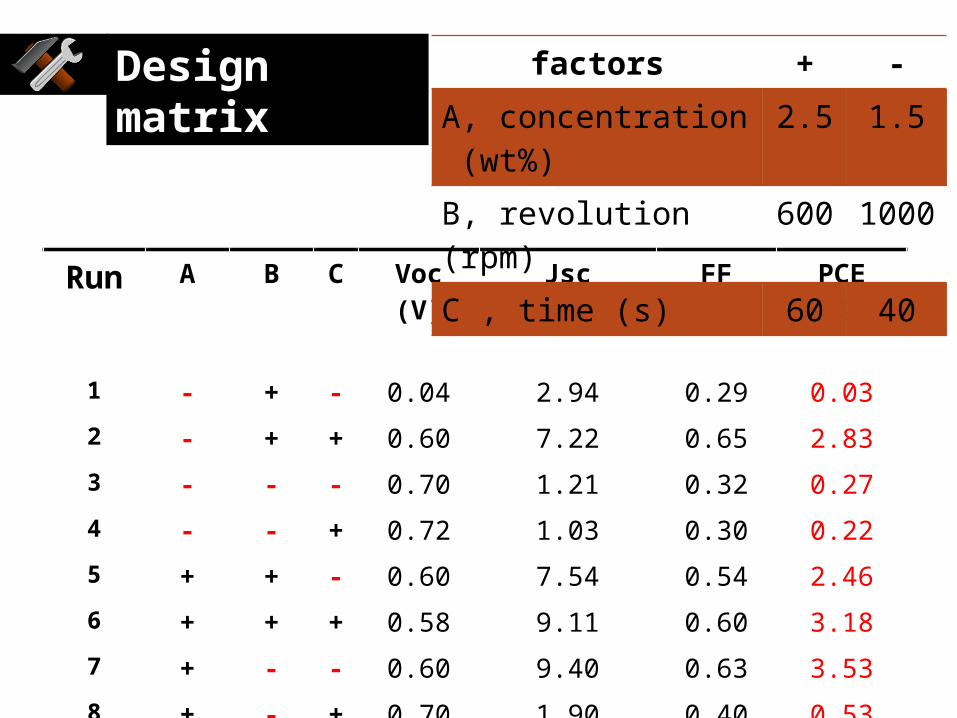
Run A B C Voc (V) Jsc (mA/cm2) FF PCE (%)

1 - + - 0.04 2.94 0.29 0.032 - + + 0.60 7.22 0.65 2.833 - - - 0.70 1.21 0.32 0.274 - - + 0.72 1.03 0.30 0.225 + + - 0.60 7.54 0.54 2.466 + + + 0.58 9.11 0.60 3.187 + - - 0.60 9.40 0.63 3.538 + - + 0.70 1.90 0.40 0.53

factors + -A, concentration  (wt%) 2.5 1.5B, revolution (rpm) 600 1000C , time (s) 60 40

Design matrix

Run A B C AB BC AC ABC PCE

1 - + - - - + + 0.03

2 - + + - + - - 2.83

3 - - - + + + - 0.27

4 - - + + - - + 0.22

5 + + - + - - - 2.46

6 + + + + + + + 3.18

7 + - - - + - + 3.53

8 + - + - - + - 0.53

effect estimateA 1.59

B 0.99

C 0.12

AB -0.20

BC 1.64

AC -1.26

ABC 0.22

The estimate of A = ( ) - ( = 1.59

Calculate the estimate