design of fluid film journal bearings containing...
TRANSCRIPT

Page 1
Design of Fluid Film Journal Bearings Containing Continuous 3D Fluid Pathways which are Formed by Wrapping a Sheet Containing 2D Through-Cut Features
by
Amos Greene Winter, V
B.S., Mechanical Engineering (2003)
Tufts University
Submitted to the Department of Mechanical Engineering in Partial Fulfillment of the Requirements for the Degree of
Master of Science in Mechanical Engineering
at the
Massachusetts Institute of Technology
June 2005
© 2005 Massachusetts Institute of Technology All rights reserved
Signature of Author………………………………………………………………………………… Department of Mechanical Engineering
May 8, 2005
Certified by………………………………………………………………………………………… Martin L. Culpepper
Rockwell International Assistant Professor of Mechanical Engineering Thesis Supervisor
Accepted by………………………………………………………………………………………... Lallit Anand
Chairman, Department Committee on Graduate Students

Page 2

Page 3
Design of Fluid Film Journal Bearings Containing Continuous 3D Fluid Pathways which are Formed by Wrapping a Sheet Containing 2D Through-Cut Features
by
Amos Greene Winter, V
Submitted to the Department of Mechanical Engineering on
May 8, 2005 in Partial Fulfillment of the Requirements for the Degree of Master of Science in Mechanical Engineering
ABSTRACT The purpose of this research was to generate the knowledge required to: (1) design and manufacture fluid film bearings that do not require precision machining processes during fabrication, but rather gain their precision from off-the-shelf parts used in the fabrication process and (2) manufacture parts with 3D internal networks by wrapping thin sheets of material containing 2D through-cut features. This wrapping-based fabrication process, called Three-Dimensional Wrapped Network (3DWN) technology, uses the precision of low-cost, ubiquitous items instead of manufacturing processes to meet the precision requirements of hydrostatic bearings. 3DWN bearings are fabricated by cutting 2D through-cut features into shim stock and then wrapping the shim stock around a precision mandrel. The 2D shim stock features are designed such that they align and form 3D internal networks within the bearing during wrapping. In the final wrapped structure the bore retains the precision diameter of the mandrel and the surface finish of the shim stock, thus meeting the functional requirements of the bearing. This thesis investigates the design and manufacturing of 3DWN hydrostatic bearings. An analytical model was derived to describe the transformation of 3D cylindrical features to 2D through-cut features. Conventional hydrostatic designs and theory were adapted for use in 3DWN bearings. A proof-of-concept was designed, constructed, and tested. Although contact between the shaft and bore was observed during testing, the fluid film stiffness matched theory within 1.6% after accounting for the contact stiffness. The mean bore diameter was measured to be within 0.03% of the mandrel diameter with errors that lie within 5σ of the tolerable error range in the front of the bearing and 2σ in the rear. In a comparison with a conventional hydrostatic bearing of the same size and surface design, the 3DWN cost 10X less. Thesis Supervisor: Martin L. Culpepper Title: Rockwell International Assistant Professor of Mechanical Engineering

Page 4
Page 5
BIOGRAPHICAL NOTE
Amos Greene Winter, V was born November 29, 1979 in Peterborough, NH. From Feb –
June 2002, he attended the University of Canterbury in Christchurch, NZ. As part of this
semester abroad, he road his motorcycle through both islands in NZ and solo through the
Australian Outback. He graduated magna cum laude from Tufts University in May 2003
with B.S in Mechanical Engineering. Starting in the fall of that year, he enrolled in the
Massachusetts Institute of Technology and joined the Precision Compliant Systems Lab
(PCSL). This thesis is the culmination of his research in the PCSL. During his masters’
degree, Amos Winter published two conference articles: “Fluid film bearings requiring
no precision machining processes, formed by wrapping 2D sheets.” ASPE 19th Annual
Meeting 2004 and “Design of a gimbaled compliant mechanism stage for precision
motion and dynamic control in Z, θX & θY directions.” ASME DETC 2004. The work
presented in this thesis is currently being prepared for publication in Precision
Engineering.

Page 6

Page 7
ACKNOWLEDGMENTS First and foremost I would like to thank Prof. Martin Culpepper for hiring, funding, and
allowing me pursue a project of my own conception. Thank you for striking the
educational balance between advising, motivating, mentoring, and giving me the freedom
to make many discoveries and mistakes on my own. You have made a profound impact
on my life, and I look forward to many fun years ahead during my PhD.
Next, I’d like to thank my labmates Spencer Szczesny and Nate Landsiedel for becoming
two of the greatest friends I have ever made, and supporting me through good times and
bad during my masters. I would also like to thank my other labmates Dariusz Golda,
Shih-Chi Chen, Kartik Mangudi, Soohyung Kim, Rich Timm, Kevin Lin, and Patrick
Carl for your help and support.
The people with whom I am closest in my personal life deserve many thanks. Thank you
Anne, for being so much more than my girlfriend by also being my best friend. Thank
you mom, Lilly, Aunie, and Darlene for your support and encouragement, and providing
a place to getaway and relax. Thank you Alex and Signe, my two lifelong friends who
have had a continuous impact on my life since elementary school. Also I want to thank
Abby, Katie Y, Brian, Chuck, Katie N, John, and Hong for your friendship.
I’d like to recognize the many professors, students, engineers and technicians who added
immense amounts to my education. Thank you Prof. Alex Slocum, Prof. Samir Nayfeh,
Prof. Tim Gutowsky, Mark Belanger, Jerry Wentworth, Maggie Sullivan, Jason Pring,
John Kane, Gil Pratt, for your technical, educational, and inspirational guidance.
Finally on a less serious note, I would like to thank all the people and things that helped
keep me sane through these last two years: My tortoise Nomar, Dave Chappelle, John
Stewart, Jerry Seinfeld, the Boston Red Sox, and my motorcycle.

Page 8

Page 9
TABLE OF CONTENTS
ABSTRACT………………………………………………………………………….........3
BIOGRAPHICAL NOTE…………………………………………………………………5
ACKNOWLEDGMENTS....……………………………………………………….……..7
TABLE OF CONTENTS.................................................................................................... 9
LIST OF FIGURES .......................................................................................................... 14
LIST OF TABLES............................................................................................................ 17
1 INTRODUCTION .....................................................................................................19
1.1 Motivation............................................................................................................ 24
1.2 Research Purpose, scope and summary of results ............................................... 27
1.2.1 Questions to be answered in research ......................................................... 28
1.2.2 Research tasks performed ........................................................................... 28
1.2.3 Scholarly contribution of research .............................................................. 29
1.2.4 Summary of results ...................................................................................... 30
1.3 Thesis Organization ............................................................................................. 31
2 BACKGROUND .......................................................................................................32
2.1 Hydrostatic bearings ............................................................................................ 32
2.1.1 How hydrostatic bearings support a load..................................................... 32
2.1.2 Modeling bearing flow................................................................................ 34
2.2 Verification of flat plate assumption in journal bearings..................................... 36
2.3 Means of fluid restriction..................................................................................... 38
2.4 Surface self-compensated bearings...................................................................... 39
3 3DWN BEARING DESIGN......................................................................................43
3.1 Inception of 3DWN technology............................................................................ 43
3.2 Early 3DWN bearing prototypes .......................................................................... 45
3.3 Motivation to design a HBP................................................................................. 45
3.4 Satisfying precision requirements of the HBP..................................................... 46
3.4.1 Characterization of surfaces........................................................................ 47
Page 10
3.4.2 Satisfying surface finish requirements........................................................ 48
3.4.3 Satisfying bore diameter and roundness requirements ............................... 49
3.5 Design of 3DWN HBP bore surface features ...................................................... 49
3.5.1 Inspiration for HBP surface feature design................................................. 50
3.5.2 HBP pad configuration ............................................................................... 51
3.5.3 Overlap region of bearing bore ................................................................... 53
3.5.4 Restrictor design ......................................................................................... 54
3.5.5 Full 3DWN HBP bore feature design ......................................................... 56
3.6 Design of Internal Channels................................................................................. 57
3.6.1 2D through-cut parameters ......................................................................... 58
3.6.2 Design of HBP fluid networks for low resistance ...................................... 59
3.6.3 Feed channel design.................................................................................... 59
3.6.4 Cross-connection channel design................................................................ 59
3.6.5 Drainage channel design ............................................................................. 60
3.7 Summary.............................................................................................................. 60
4 MODELING AND ANALYSIS................................................................................61
4.1 Wrapping model................................................................................................... 61
4.1.1 Describing a wrapped structure .................................................................. 61
4.1.2 3D to 2D coordinate transformation ........................................................... 65
4.2 Modeling bearing performance............................................................................ 70
4.2.1 Fluid resistance modeling ............................................................................ 70
4.2.2 Resistance ratio ............................................................................................ 72
4.2.3 Derivation of effective pad area................................................................... 73
4.2.4 Derivation of bearing stiffness..................................................................... 75
4.3 Sensitivity Analysis .............................................................................................. 76
4.3.1 Justification for using non-precision cutting processes .............................. 76
4.3.2 Sensitivity of performance to internal channel errors................................. 78
4.3.3 Justification for neglecting tension in the wrapping model ........................ 80
4.3.4 Sensitivity to bore bulge to channel placement .......................................... 81
4.3.5 Appropriate wrapping tension to compress Template deformities ............. 82
4.4 Summary............................................................................................................... 83

Page 11
5 MANUFACTURING A 3DWN HBP .......................................................................84
5.1 Failed attempts at adhering wrapped layers......................................................... 84
5.2 Template fabrication ............................................................................................ 86
5.2.1 Waterjet cutting........................................................................................... 86
5.2.2 Fixturing of Template within waterjet ........................................................ 87
5.3 Template wrapping .............................................................................................. 87
5.3.1 Rolling jig ................................................................................................... 87
5.3.2 Alignment of Template to mandrel............................................................. 88
5.3.3 Adhesion of wrapped layers........................................................................ 90
5.4 Packaging the Template in a housing .................................................................. 91
5.4.1 Joining Template and housing .................................................................... 91
5.4.2 Prepping the HBP for casting ..................................................................... 92
5.4.3 Casting the Template into the housing........................................................ 93
5.4.4 Finishing procedures................................................................................... 94
5.5 Summary............................................................................................................... 95
6 EXPERIMENTAL VERIFICATION........................................................................96
6.1 Experimental setup............................................................................................... 96
6.5.1 Parameters of the 3DWN HBP used in experimentation............................ 96
5.1.2 Experimental setup for stiffness testing...................................................... 98
5.1.3 Bore measurement ....................................................................................... 99
5.2 Stiffness results and discussion........................................................................... 100
5.2.1 Stiffness test results.................................................................................... 100
5.2.2 Sources of error in stiffness data................................................................ 101
5.3 Results from bore measurements ........................................................................ 104
5.4 Cost comparison.................................................................................................. 104
5.5 Summary............................................................................................................. 105
7 SUMMARY.............................................................................................................106
7.1 Scholarly Contributions ..................................................................................... 106
7.2 Engineering impact ............................................................................................ 107
7.3 Future work........................................................................................................ 108

Page 12
REFERENCES................................................................................................................110

Page 13
Page 14
LIST OF FIGURES
Figure 1.1 3DWN bearing manufacturing process ........................................................... 21
Figure 1.2 Precision requirements decoupled from fabrication of the bearing................ 22
Figure 1.3 Finished 3DWN bearing.................................................................................. 23
Figure 2.1 Configurations and pressure profiles for different bearings........................... 33
Figure 2.2 Fluid relationships in hydrostatic bearings..................................................... 34
Figure 2.3 Velocity profile of fully developed flow........................................................ 34
Figure 2.4 Bearing eccentricity during shaft displacement ............................................. 37
Figure 2.6 HydroglideTM surface self-compensated bearing [1]...................................... 41
Figure 2.7 Fluid circuit for surface self-compensated bearing ........................................ 41
Figure 3.1 Flat actuator concept and implementation...................................................... 44
Figure 3.2 First 3DWN mock-up and rolling process...................................................... 44
Figure 3.3 Example surface roughness profile [20]......................................................... 47
Figure 3.4 Determination of Ra value [21]...................................................................... 48
Figure 3.5 Hydrostatic self-compensated journal bearing [22] ....................................... 50
Figure 3.6 Annular restrictor designs for hydrostaic surface self-compensated bearings 51
Figure 3.7 Comparison of pad configurations ................................................................. 52
Figure 3.8 Chosen 3DWN HBP bore surface features layout ......................................... 53
Figure 3.9 Geometric matching of overlap region........................................................... 54
Figure 3.10 Single feed, double annulus restrictor configuration.................................... 55
Figure 3.11 3DWN self-compensated bearing pad bore surface features and geometric
parameters ................................................................................................................. 56
Figure 3.12 3DWN self-compensated bearing template................................................... 58
Figure 4.1 Diagram of overlap region of layer one and two............................................ 62
Figure 4.2 Model used for x-displacement of cantilevered beam.................................... 64
Figure 4.3 Transformation of 3D cylindrical features to Template features ................... 66
Figure 4.4 Local coordinate system for position along cantilevered beam ..................... 67
Figure 4.5 Flow over bearing bore surface features ........................................................ 71
Figure 4.6 Fluid circuit of one set of opposed pads in the HBP ...................................... 71
Figure 4.7 Pressure profile over bearing pad ................................................................... 73

Page 15
Figure 4.8 Pad stiffness configuration of HBP (gap greatly exaggerated) ...................... 75
Figure 4.9 Sensitivity of the HBP stiffness to manufacturing errors for h/R = .002, h/l =
0.011.......................................................................................................................... 77
Figure 4.10 Channel constriction as a result of internal feature misalignment ............... 78
Figure 4.11 Internal channel resistance sensitivity to expected error range of t and R for
t/R = 0.01................................................................................................................... 79
Figure 4.12 Error caused by wrapping tension ................................................................. 81
Figure 4.13 Bore bulge resulting from pressurized channels .......................................... 81
Figure 4.14 Deflection of Template due to tension ......................................................... 82
Figure 4.15 FEA Results from deformity deflection under tension ................................ 83
Figure 5.1 Template being cut in waterjet ....................................................................... 86
Figure 5.2 Kinematic fixture for waterjet cutting, waterjet cutting setup........................ 87
Figure 5.3 3DWN bearing rolling jig............................................................................... 88
Figure 5.4 Template mounted on rolling jig .................................................................... 89
Figure 5.5 Adhering adjacent layers within the HBP ...................................................... 91
Figure 5.6 Centering of Template within housing ........................................................... 92
Figure 5.7 Preparations for casting .................................................................................. 93
Figure 5.8 Wrapped Template cast in housing ................................................................ 94
Figure 5.9 Drainage ports with grease plugs removed .................................................... 94
Figure 5.10 Residual super glue to be removed from bearing bore surface features....... 95
Figure 6.1 Experimental setup for testing stiffness .......................................................... 98
Figure 6.2 Oil pressurization device ................................................................................ 99
Figure 6.3 Bore precision testing using a CMM............................................................ 100
Figure 6.4 Measured stiffness vs. theory ....................................................................... 101
Figure 6.5 View of leakage flow (shaft removed from bore) ........................................ 102
Figure 6.6 Bearing fluid circuit including leakage flow................................................ 102
Figure 6.7 Theoretical stiffness with and without leaks ................................................. 103

Page 16

Page 17
LIST OF TABLES
Table 1.1 Comparison of different bearing types [2]....................................................... 24
Table 1.2 Hydrostatic journal bearing applications [1-3] ................................................ 25
Table 2.1 Methods of bearing compensation................................................................... 39
Table 3.1 Progression of early 3DWN prototypes........................................................... 45
Table 5.1 Failed attempts at adhering wrapped layers..................................................... 85
Table 6.1 Parameters of the 3DWN HBP used in experimention.................................... 97
Table 6.2 Measurements of bore at front and rear of bearing........................................ 104
Table 6.3 Cost comparison 3DWN and conventional bearing ...................................... 105

Page 18
Page 19
CHAPTER
1 INTRODUCTION
The purpose of this research was to generate the knowledge required to:
1. Design and manufacture fluid film bearings (FFBs) that do not require precision
machining processes during fabrication, but rather gain their precision from off-
the-shelf parts used in the fabrication process.
2. Manufacture parts with 3D internal networks by wrapping thin sheets of material
containing 2D through-cut features.
All FFBs support a load on a pressurized film of fluid. The bearing surfaces have to be
precise in their spacing and surface finish to insure uniform film properties and to insure
no mechanical contact between bearing components. Traditional FFBs require precision
machining processes to provide the requisite geometric accuracy and surface finish.
Additionally, fluid static bearings require internal networks to distribute fluid throughout
the bearing. Current FFBs have the following drawbacks which limit their use in
widespread engineering applications:
• Precision machining processes used to make the bearing surface contribute
significantly to the overall cost of the bearing.
• Fluid networks have to be machined or cast into the bearing, which adds extra
labor time, manufacturing steps, and cost to the bearing.

Page 20
• Fixed restrictor bearings require tuning for optimum performance (means of
restriction are discussed in a later section), adding further labor time and effort
during bearing installation.
• Self-compensated bearings, which self-tune and can achieve twice the stiffness of
fixed restrictor bearings [1], require extensive internal channels which connect
restrictors and pads.
The central thesis of this research is that FFBs can be fabricated with incorporated
internal networks by wrapping thin 2D sheets. Further, this may be accomplished
without the need for a bearing manufacturer to perform precision machining processes.
This wrapping-based fabrication process, called Three-Dimensional Wrapped Network
(3DWN) technology, uses the precision of low-cost, ubiquitous items instead of
manufacturing processes to meet the precision requirements of the bearing. Figure 1.1
illustrates how 3DWN bearings are made.

Page 21
Step Process
1
Precision diameter
ground mandrel
Precision surface finish
and thickness material
(e.g. shim stock)
Precision diameter
ground mandrel
Precision surface finish
and thickness material
(e.g. shim stock)
2 Template cut into shim stock with 2D process
(e.g. laser cutting)
Adhesive applied to back side
Template cut into shim stock with 2D process
(e.g. laser cutting)
Adhesive applied to back side
3 Template wrapped about mandrel
Adhesive bonds
each layer
Template wrapped about mandrel
Adhesive bonds
each layer
Fin
ish
3DWN
bearing
3DWN
bearing
Precision
surface finish
from shim
stock
Precision
diameter from
mandrel
Precision
surface finish
from shim
stock
Precision
diameter from
mandrel
3D internal
features
formed by
template
3D internal
features
formed by
template
Figure 1.1 3DWN bearing manufacturing process
The 3DWN process begins with two off-the-shelf parts that have inherent precision:

Page 22
1. A precision ground mandrel with the required diameter size, tolerance, and
circularity for the bearing
2. Cold rolled shim stock with the required surface finish for the bearing
A pattern of through-cut features is cut into the shim stock, forming a template. Adhesive
is applied to the back of the template. The features in the template are designed such that
they form internal networks within the bearing when the template is wrapped. In its final
form, the bearing bore retains the precision diameter of the mandrel and the surface finish
of the shim stock, thus meeting the functional requirements of the bearing.
3DWN bearings can be made less expensively than conventional hydrostatic journal
bearings given that the precision requirements of the bearing are satisfied by low-cost,
well-developed manufacturing processes. The chart in Figure 1.2 demonstrates how the
precision of the bearing is decoupled from the fabrication of the bearing.
Off-the-shelf shim
stock with cold rolled
precision surface finish
Off-the-shelf precision
ground mandrel
Precision parts
Off-the-shelf shim
stock with cold rolled
precision surface finish
Off-the-shelf precision
ground mandrel
Precision parts
Wrapping
Waterjet or laser
cutting
Non-precision
processes
Wrapping
Waterjet or laser
cutting
Non-precision
processes
[1,6]
When wrapped, 2D cut
features in adjacent layers
align to form internal
networks
Fluid networked between
input, restrictors, pads, and
drains
Bearing features cut into
Template using 2D through-
cutting process
Restrictors, pads, and drains
cut in bore surface
Template, made from shim
stock with precision surface
finish, forms bore surface
The maximum peak-to-
valley surface roughness not
greater than one-fourth the
bearing gap
Template wrapped around
precision ground mandrel,
replicating mandrel diameter
Design ParametersFunctional Requirements
When wrapped, 2D cut
features in adjacent layers
align to form internal
networks
Fluid networked between
input, restrictors, pads, and
drains
Bearing features cut into
Template using 2D through-
cutting process
Restrictors, pads, and drains
cut in bore surface
Template, made from shim
stock with precision surface
finish, forms bore surface
The maximum peak-to-
valley surface roughness not
greater than one-fourth the
bearing gap
Template wrapped around
precision ground mandrel,
replicating mandrel diameter
Total diameter errors
within one-forth of
bearing gap
Design ParametersFunctional Requirements
Figure 1.2 Precision requirements decoupled from fabrication of the bearing

Page 23
3DWN technology enables greater flexibility in design because many sizes of 3DWN
bearings can be made with the same process. For instance, a 3DWN bearing assembly
line equipped with one wrapping machine and a variety of mandrel sizes could produce
multiple bearing designs and sizes. Mandrels could be re-used between bearings, which
could further reduce the cost of production.
A self-compensated hydrostatic journal bearing, shown in Figure 1.3, was designed,
modeled, and tested as a case study for 3DWN technology. This bearing is composed of
two sets of four radial pads, which give the bearing moment and radial stiffness. The
template contains all bearing features and internal fluid networking, including feed, drain,
and cross channeling between the restrictors and pads. The 3DWN bearing is potted
within an aluminum sleeve. In this form, the quasi-monolithic assembly is structurally
stiff. The housing allows for mounting and provides a connection to pressurized fluid.
Restrictor
Pad Pocket
Drainpocket
Wrappedbearing
Pottingcompound
Aluminumsleeve
A. Bearing after wrapping B. Bearing cast into an aluminum housing
Figure 1.3 Finished 3DWN bearing
The bearing shown in Figure 1.3 is a proof-of-concept, and is not designed for any
specific application. This thesis presents the design process, modeling, and fabrication
used to make the prototype shown in Figure 1.3. The methods described may be used by
engineers to design 3DWN bearings for specific applications.
Page 24
1.1 Motivation
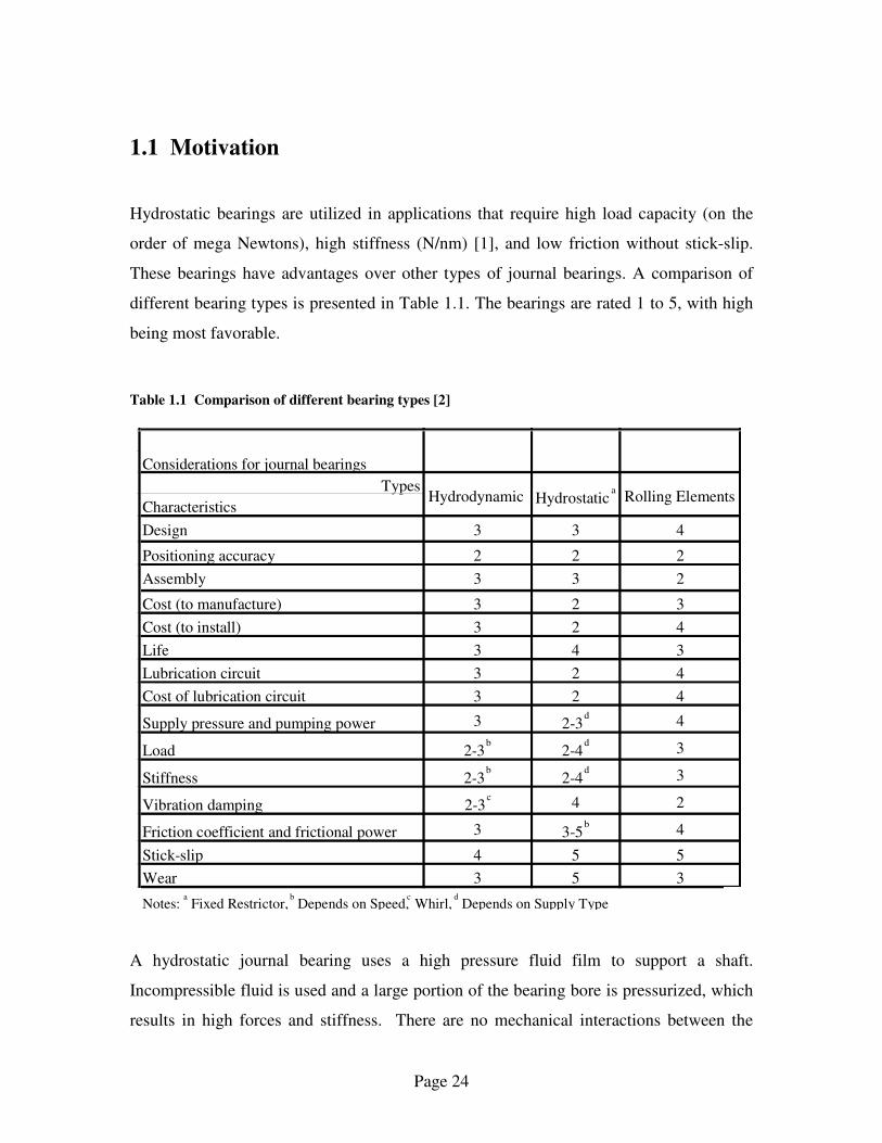
Hydrostatic bearings are utilized in applications that require high load capacity (on the
order of mega Newtons), high stiffness (N/nm) [1], and low friction without stick-slip.
These bearings have advantages over other types of journal bearings. A comparison of
different bearing types is presented in Table 1.1. The bearings are rated 1 to 5, with high
being most favorable.
Table 1.1 Comparison of different bearing types [2]
Types
Characteristics
Design 3 3 4
Positioning accuracy 2 2 2
Assembly 3 3 2
Cost (to manufacture) 3 2 3
Cost (to install) 3 2 4
Life 3 4 3
Lubrication circuit 3 2 4
Cost of lubrication circuit 3 2 4
Supply pressure and pumping power 3 2-3d 4
Load 2-3b
2-4d 3
Stiffness 2-3b
2-4d 3
Vibration damping 2-3c 4 2
Friction coefficient and frictional power 3 3-5b 4
Stick-slip 4 5 5
Wear 3 5 3
Notes: a
Fixed Restrictor, b
Depends on Speed, c
Whirl, d
Depends on Supply Type
Considerations for journal bearings
Hydrodynamic Hydrostatica
Rolling Elements
A hydrostatic journal bearing uses a high pressure fluid film to support a shaft.
Incompressible fluid is used and a large portion of the bearing bore is pressurized, which
results in high forces and stiffness. There are no mechanical interactions between the

Page 25
shaft and the bearing bore since the shaft is completely supported on the fluid film. As a
result there is no stick-slip, making the motion of the bearing highly repeatable.
Hydrostatic bearings are ideal for applications where high load capacity, high stiffness,
and low friction are needed. Unlike hydrodynamic bearings, hydrostatic bearings do not
require a spinning shaft to maintain their load-bearing properties. As such, they have
excellent performance in stationary and stop-start operation. Table 1.2 lists specific
applications and benefits of hydrostatic journal bearings.
Table 1.2 Hydrostatic journal bearing applications [1-3]
Telescopes
Radio telescopes
Radar antennas
Air preheaters for boilers
Rotating mills for ores or slags
Large boring machines
Large milling machines
Large lathes
Assembly lines
Large structures
Grinding machines
CNC machining centers
Medium-high velocity spindles
Precision balances
Dynamometers
Vibration attenuators
Frictionless oil seals
Small machines
Medium sized machines
Large machines
High load capacity
No wear
Precision rotation
Squeeze film damping
High stiffness
No stick-slips
Lubricated while stopped
No wear
Near zero friction at low
speed
Categories Specific applications Benefits
Hydrostatic journal bearing applications
Hydrostatic journal bearings offer better performance than other types of bearings.
However, there are factors that make them undesirable for some applications:

Page 26
• Bore machining cost: Traditional hydrostatic journal bearings require a precision
process to machine the bore to the required diameter and surface finish.
• Fluid channel machining cost: Hydrostatic bearings require fluid to be injected
into multiple locations between the bore and shaft. Distribution of fluid requires
an internal network system around the bearing.
• Added machining for self compensation: Self compensating bearings offer higher
load capacities and stiffness than fixed compensator bearings, but require
additional fabrication to produce cross-linked fluid pats for restrictors and pads.
• Custom design and low production volume: Hydrostatic bearings can vary in and
size and surface feature layout, requiring most designs to be customized and made
in small numbers.
Methods have been employed to lower the cost of producing hydrostatic journal bearings,
yet all of these require at least one precision machining process. Self-compensated
hydrostatic journal bearings, made by Kotilainen, et al. [4,5], were formed by sand or
investment casting. Although these bearings require fewer manufacturing steps than
conventional FFBs, the bore requires post-casting precision machining post and the
molds are destroyed during production, which further adds cost.
Kotilainen’s cast bearings are a spin-off from a reduced-cost technology, the
TurboToolTM and HydroSpindleTM [6-9], which have the bearing features cut into the
shaft instead of the bearing bore. These technologies still require 3D machining and
precision grinding of the shaft. Another method of making hydrostatic bearings is by
pressing bronze sleeves into a block. In this process the bore has to be post machined to
compensate for the press fitting [10]. Also, Babbitting, where molten metal is cast around
a conical shaft, has been used for decades to make replicated bores, but this process also
requires finish machining [10, 11]. Polymers have been through-cut with a bearing bore

Page 27
surface features and adhered to bearing bores [Lyon patent], but this process requires the
bore to be machined to same diameter precision as a conventional hydrostatic bearing.
Kotilainen’s research demonstrates that an imprecise process such as casting may be used
to make the bearing bore surface bore surface features without adversely affecting
performance. This reduces the cost of producing these bearings below that of
conventional bearings [4,5]. In a similar fashion 3DWN technology uses imprecise
through-cutting processes like laser or waterjet cutting to make the bearing features. As
such, the precision requirements may be met by off-the-shelf parts. The advantages of
3DWN technology in bearing manufacturing are summarized below.
• Decoupled precision: The precision requirements of the bearing are
compartmentalized within the mandrel and shim stock, which are low cost and
easy of others to fabricate. Cutting of the template does not require a precision
process.
• Included feed channels: Bearing features and internal network features are all
included in the template.
• 1-Step machining: Using 3DWN technology, the bearing features and the network
features are cut in the template at the same time using the same process.
• Monolithic construction: 3DWN wrapped structures are made from one part, and
may easily be potted into a housing to make a bearing.
• Flexible production: The mandrel is not destroyed during the wrapping process.
Thus, a single wrapping system with multiple mandrels may make varying
bearing sizes.
1.2 Research Purpose, scope and summary of results
Page 28
1.2.1 Questions to be answered in research
The questions that are answered through this research are:
1. How can a cylindrical structure with internal features be modeled as a wrapped
structure, and how is the wrapped structure modeled unrolled as a 2D sheet with
through-cut features? What errors result that affect bearing performance result
from this process?
2. How is the level of precision quantified for the off-the-shelf parts used in 3DWN
bearing fabrication?
3. How are 3DWN bearings manufactured? What bearing materials, adhesives, and
support structures have to be considered in implemented. What is the best method
for rolling?
4. What are the practical issues regarding the design process, fabrication, and
implementation of 3DWN technology to fluid film bearings?
5. How can a 3DWN bearing design be chosen for a particular application? What
modeling techniques are necessary to select a 3DWN bearing design, determine
its dimensions, and predict its performance?
1.2.2 Research tasks performed
These questions were answered through the following research tasks:
Page 29
1. A model to transform 3D cylindrical coordinates to 2D sheet coordinates was
derived. Errors were introduced into the model and resulting sensitivity to bearing
performance was analyzed.
2. Conventional bearing theory for precision requirements was used to form metrics
for off-the-shelf precision parts.
3. Materials suitable to wrapping and use in the bearing were determined. Multiple
adhesives were tested. Prototypes to verify manufacturing methods were built.
4. Current fluid film bearing theory and bearing feature designs were modified for
use in 3DWN bearings.
5. A 3DWN bearing prototype was built and tested as a bench-level prototype.
1.2.3 Scholarly contribution of research
The following scholarly contributions are a result of the work presented in this thesis:
1. 3DWN technology is a new method of making a precision bearing bore. Surface
replication by wrapping is a deviation from conventional bearing manufacturing
practices; all current fluid film journal bearings require at least one precision
process in their construction.
2. In the 3DWN manufacturing process the errors associated with the non-precision
parts have less of an effect on bearing performance then errors in the precision
parts. This is a powerful relationship, in that it supports the feasibility of 3DWN
technology by showing a hydrostatic bearing’s precision requirements can be
decoupled from the fabrication processes used to make it.

Page 30
3. Metrics to judge the level of precision required in the off-the-shelf parts used to
make a 3DWN bearing are defined from conventional hydrostatic bearing theory.
4. A new method of manufacturing 3D parts with internal features by using 3DWN
technology. 3DWN is not limited to fluid channels; it could be used for many
kinds of applications that require cylindrical internal networks.
5. A model for describing a wrapped structure is derived. This model enables
coordinates in a 3D cylindrical structure to be transformed to a 2D Template.
When the Template is rolled, the 2D features align in the wrapped structure to
recreate the original 3D features.
6. Existing bearing features are modified such that it can be cut into a 2D Template.
Conventional hydrostatic bearing analysis is used to evaluate the bearing
performance.
1.2.4 Summary of results
The final 3DWN bearing prototype designed, constructed, and tested for this thesis was a
surface self-compensated hydrostatic journal bearing. The bearing had a bore surface
features consists of two axial sets of four circumferentially spaced pads, each connected
to an opposed surface restrictor. It was lubricated with heavy weight motor oil and
pressurized with shop air regulated to a safe level (100psi) for laboratory experiment.
Load capacity and stiffness were tested by applying varying loads to the shaft and
measuring the eccentricity of the shaft within the bearing.
Although contact between the shaft and bore was observed, the fluid film stiffness
matched theory within 1.6% after accounting for the contact stiffness. The mean bore
diameter was measured to be within 0.03% of the mandrel diameter with errors that lie
within 5σ of the tolerable error range in the front of the bearing and 2σ in the rear. In a
Page 31
comparison with a conventional hydrostatic bearing of the same size and surface design,
the 3DWN cost 10X less.
1.3 Thesis Organization
Chapter 2 presents a background on hydrostatic bearings, which includes modeling of
bearing fluid flow and means of restriction. The third chapter describes how the concept
for 3DWN bearings was conceived and how 3DWN bearings are designed. The fourth
chapter presents the wrapped structure model, error functions, the use of established
bearing theory in 3DWN bearings, and a cost comparison with conventional hydrostatic
journal bearings. The fifth chapter describes the materials and adhesives were chosen and
how 3DWN bearing prototypes were constructed. The experimental setup, testing
procedure, and results are presented in the sixth chapter. Possible sources of error are also
identified and verified through testing and examination. The seventh chapter provides a
summary of results and a discussion of future research.

Page 32
CHAPTER
2 BACKGROUND
This chapter covers the basic theory behind hydrostatic bearings. The first section
provides an explanation of how a hydrostatic bearing supports a load. The second section
presents verification the flat plate model used in journal bearings. The third section
describes methods of restricting bearing flow. The final section gives a background on
surface self-compensated bearings.
2.1 Hydrostatic bearings
2.1.1 How hydrostatic bearings support a load
Hydrostatic bearings support a load on a thin film of pressurized fluid. The origins of
these bearings can be traced to L.G. Girard, who in 1852 made the first water hydrostatic
journal bearing [13]. In all hydrostatic bearings, pressurized fluid is pumped into the pad
and slowly flows out over the bearing lands. The bearing gap is small enough to restrict
the flow over the lands and induce a linear pressure drop from viscous losses. Depending
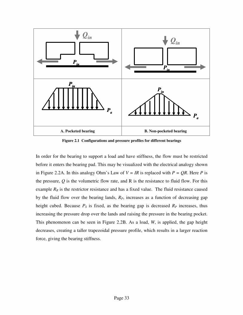
on whether or not the bearing is pocketed, the pressure profile over the bearing surface
has a triangular or trapezoidal pressure profile, as shown in Figure 2.1. A pocketed
bearing has the benefit of a larger area exposed to input pressure, thus resulting in higher
load capacity and stiffness
Page 33
Qin
Pin
Qin
Pin P
in
Qin
Pin
Qin
Pin
Pa
Pin
Pin
Pa
Pin
Pa
Pin
Pa
A. Pocketed bearing B. Non-pocketed bearing
Figure 2.1 Configurations and pressure profiles for different bearings
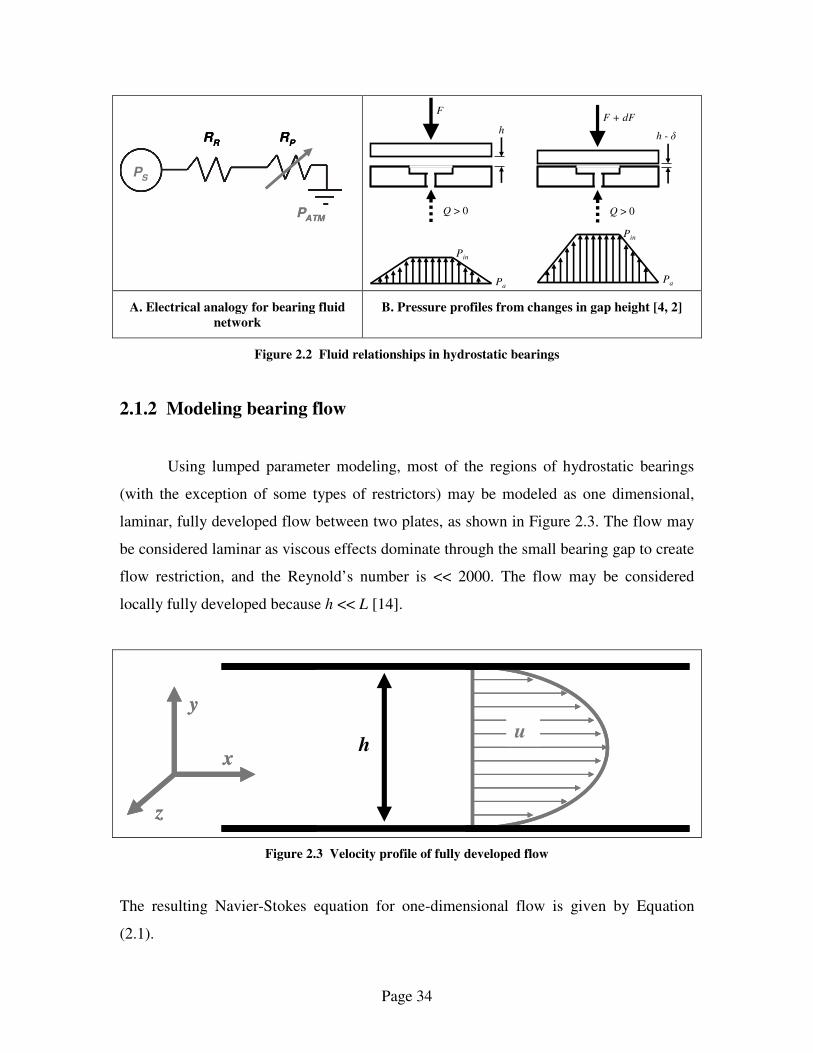
In order for the bearing to support a load and have stiffness, the flow must be restricted
before it enters the bearing pad. This may be visualized with the electrical analogy shown
in Figure 2.2A. In this analogy Ohm’s Law of V = IR is replaced with P = QR. Here P is
the pressure, Q is the volumetric flow rate, and R is the resistance to fluid flow. For this
example RR is the restrictor resistance and has a fixed value. The fluid resistance caused
by the fluid flow over the bearing lands, RP, increases as a function of decreasing gap
height cubed. Because PS is fixed, as the bearing gap is decreased RP increases, thus
increasing the pressure drop over the lands and raising the pressure in the bearing pocket.
This phenomenon can be seen in Figure 2.2B. As a load, W, is applied, the gap height
decreases, creating a taller trapezoidal pressure profile, which results in a larger reaction
force, giving the bearing stiffness.
Page 34
RR
RP
PATM
PS
RR
RP
PATM
PS
h
Q > 0
F
Q > 0
F + dF
h - δ
Pa
Pin
Pa
Pin
A. Electrical analogy for bearing fluid network
B. Pressure profiles from changes in gap height [4, 2]
Figure 2.2 Fluid relationships in hydrostatic bearings
2.1.2 Modeling bearing flow
Using lumped parameter modeling, most of the regions of hydrostatic bearings
(with the exception of some types of restrictors) may be modeled as one dimensional,
laminar, fully developed flow between two plates, as shown in Figure 2.3. The flow may
be considered laminar as viscous effects dominate through the small bearing gap to create
flow restriction, and the Reynold’s number is << 2000. The flow may be considered
locally fully developed because h << L [14].
y
x
z
hu
y
x
z
hu
Figure 2.3 Velocity profile of fully developed flow
The resulting Navier-Stokes equation for one-dimensional flow is given by Equation
(2.1).

Page 35
(2.1)
Equation (2.1) can be reduced using the following assumptions:
1. During operation under constant supply pressure, the flow is steady.
2. Since hydrostatic bearings use incompressible fluids, mass conservation though a
uniform bearing gap requires that the velocity in the x direction be constant.
3. There can not be any flow through the walls of the bearing gap, so there is no
flow in the y direction.
4. The flow is uniform and does not vary in the z direction.
5. Horizontal height changes are negligible, so body forces can be ignored.
The reduced Navier-Stokes equation is given by Equation (2.2).
dx
dp
dy
ud=
2
2
µ (2.2)
Integrating Equation (2.2) twice and applying the non-slip boundary conditions of
u(0)=u(h)=0, yields Equation (2.3) for the flow velocity.
xgx
pu
zu
yu
xz
uw
y
uv
x
uu
t
uρµρ +
∂
∂−
∂
∂+
∂
∂+
∂
∂=
∂
∂+
∂
∂+
∂
∂+
∂
∂2
2
2
2
2
2
1 2 3 4 2 4 5

Page 36
)(2
1yhy
dx
dpu −
=
µ (2.3)
Integrating the velocity over the entrance area of the bearing, which is defined by the
height and width of the land, results in Equation (2.4) for the volumetric flow rate.
=
dx
dphwQ
µ12
3
(2.4)
Where w is the width of the land. To express pressure, flow rate, and flow resistance in
the analogous form of V = IR, the pressure can be integrated over the land length L to
obtain Equation (2.5).
wh
L
Q
pR
3
12µ=
∆= (2.5)
This expression is powerful because it can be used to express all the geometric
parameters of the bearing as a fluid resistance. As such, the bearing may be modeled with
lumped parameters, with each parameter being composed of variations of Equation (2.5).
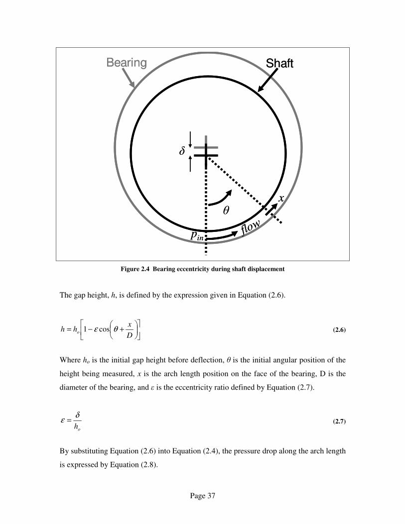
2.2 Verification of flat plate assumption in journal bearings
A problem arises when using the flat plate approximation for journal bearings: journal
bearings are not flat. Figure 2.4 shows a displaced shaft within a journal bearing. As a
result of the curvature of the bearing, the gap does not decrease uniformly. Modeling
flow in a uniform gap is much simpler than in a varying gap, thus a flat plate
approximation is advantageous if it doesn’t deviate significantly from the curved plate
model. This section will investigate the error associated with using the flat plate
approximation instead of a curved plate model. The method used was adapted from [4,6]
Page 37
δ
θx
pinflo
w
Bearing Shaft
δ
θx
pinflo
w
Bearing Shaft
Figure 2.4 Bearing eccentricity during shaft displacement
The gap height, h, is defined by the expression given in Equation (2.6).
+−=
D
xhh o θε cos1 (2.6)
Where ho is the initial gap height before deflection, θ is the initial angular position of the
height being measured, x is the arch length position on the face of the bearing, D is the
diameter of the bearing, and ε is the eccentricity ratio defined by Equation (2.7).
oh
δε = (2.7)
By substituting Equation (2.6) into Equation (2.4), the pressure drop along the arch length
is expressed by Equation (2.8).

Page 38
3
3cos1
112
+−
−=
D
xh
w
Q
dx
dp
o θε
µ
(2.8)
the ratio L
x=ξ may be used to find the pressure drop along the arch length from
Equation (2.8) using a definite integral. The resulting flow resistance in the
circumferential direction is given by Equation (2.9).
∫−
+−
=2
1
2
133
cos1
112ξ
ξθε
µd
D
Lwh
LR
o
(2.9)
It is important to note that the ratio L/D is different than the usual L/D ratio that
corresponds to the bearing length and diameter. In Equation (2.9) L/D is the ratio of the
land length and the diameter. Dividing Equation (2.9) by Equation (2.5) and evaluating at
L/D = 0.1, which is a realistic approximation [4], and an eccentricity of 0.5, which
corresponds to the operating range of a typical bearing [2], the ratio of resistances at any
radial position around the pad, θ = 0o to 90o, is very small (<1%). Thus, the flat plate
approximation may be used to accurately model fluid film journal bearings.
2.3 Means of fluid restriction
As mentioned previously, restrictors are required in bearing fluid circuits. They induce a
pressure drop in the fluid as it enters the bearing pad. When the resistance of the bearing
lands increases, the pressure in the bearing pad increases. The bearing has stiffness
because the load capacity increases with bearing displacement.
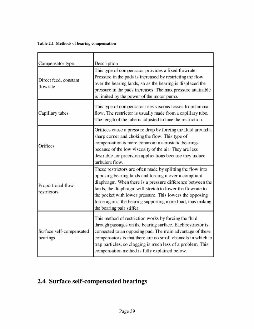
Table 2.1 describes different types of restrictors that are commonly used. This table is a
summary of information on restrictors from [1,2].
Page 39
Table 2.1 Methods of bearing compensation
Direct feed, constant
flowrate
This type of compensator provides a fixed flowrate.
Pressure in the pads is increased by restricting the flow
over the bearing lands, so as the bearing is displaced the
pressure in the pads increases. The max pressure attainable
is limited by the power of the motor pump.
Capillary tubes
This type of compensator uses viscous losses from laminar
flow. The restrictor is usually made from a capillary tube.
The length of the tube is adjusted to tune the restriction.
Orifices
Orifices cause a pressure drop by forcing the fluid around a
sharp corner and choking the flow. This type of
compensation is more common in aerostatic bearings
because of the low viscosity of the air. They are less
desirable for precision applications because they induce
turbulent flow.
Proportional flow
restrictors
These restrictors are often made by splitting the flow into
opposing bearing lands and forcing it over a compliant
diaphragm. When there is a pressure difference between the
lands, the diaphragm will stretch to lower the flowrate to
the pocket with lower pressure. This lowers the opposing
force against the bearing supporting more load, thus making
the bearing pair stiffer.
Surface self-compensated
bearings
This method of restriction works by forcing the fluid
through passages on the bearing surface. Each restrictor is
connected to an opposing pad. The main advantage of these
compensators is that there are no small channels in which to
trap particles, so clogging is much less of a problem. This
compensation method is fully explained below.
Compensator type Description
2.4 Surface self-compensated bearings
Page 40
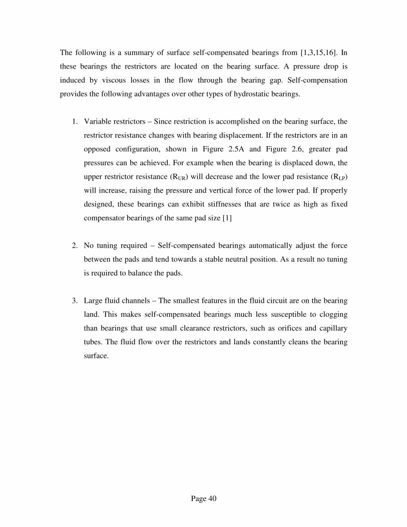
The following is a summary of surface self-compensated bearings from [1,3,15,16]. In
these bearings the restrictors are located on the bearing surface. A pressure drop is
induced by viscous losses in the flow through the bearing gap. Self-compensation
provides the following advantages over other types of hydrostatic bearings.
1. Variable restrictors – Since restriction is accomplished on the bearing surface, the
restrictor resistance changes with bearing displacement. If the restrictors are in an
opposed configuration, shown in Figure 2.5A and Figure 2.6, greater pad
pressures can be achieved. For example when the bearing is displaced down, the
upper restrictor resistance (RUR) will decrease and the lower pad resistance (RLP)
will increase, raising the pressure and vertical force of the lower pad. If properly
designed, these bearings can exhibit stiffnesses that are twice as high as fixed
compensator bearings of the same pad size [1]
2. No tuning required – Self-compensated bearings automatically adjust the force
between the pads and tend towards a stable neutral position. As a result no tuning
is required to balance the pads.
3. Large fluid channels – The smallest features in the fluid circuit are on the bearing
land. This makes self-compensated bearings much less susceptible to clogging
than bearings that use small clearance restrictors, such as orifices and capillary
tubes. The fluid flow over the restrictors and lands constantly cleans the bearing
surface.

Page 41
A. Fluid circuit of opposed pads B. HydroglideTM topology
Figure 2.5 HydroglideTM surface self-compensated bearing [1]
Ps
RUR
RLPRLR
RUP
RLL
RUL
PA
Figure 2.6 Fluid circuit for surface self-compensated bearing
The HydroglideTM, shown in Figure 2.5, is a unique design in self-compensated bearings
because the resistance of the restrictor is deterministic. Fluid flows from an outer annulus
radially inwards to a center hole, shown in Figure 2.5A. This configuration is different

Page 42
from early restrictor designs, where fluid flows outwards from a source to collection
pockets [3,16]. The HydroglideTM is easier to model than other self-compensated
bearings because the bearing flow is in the opposite direction of leakage flow, making
leakage not affect bearing performance.

Page 43
CHAPTER
3 3DWN BEARING DESIGN This chapter presents the process used to design the 3DWN HBP. The chapter begins
with the inception and evolution of 3DWN technology then focuses on the design of the
most recent 3DWN surface self-compensated HBP. The design process is composed of
three stages: 1) satisfying the precision requirements of the HBP, 2) modifying existing
bearing technology for incorporation into a wrapped structure, and 3) designing the
remainder of the Template to include internal networks. Qualitative design choices based
upon sound engineering knowledge compose the majority of this chapter. Quantitative
methods behind design decisions are mentioned in this chapter with the full analysis
explained in Chapter 4.
3.1 Inception of 3DWN technology
3DWN technology grew out of research on flat pneumatic and hydraulic actuators. The
initial objective of that project was to research the feasibility of making flat, monolithic
pneumatic and hydraulic actuators with pistons, actuator bodies, return spring
mechanisms, and fluid routing channels. The actuators were designed to have fluid film
bearings on the piston surfaces to reduce friction, as shown in (Figure 3.1 A). The bearing
gaps were created by compliant end caps, which expanded when the piston was
pressurized. A goal of the project was to enable the production of monolithic robot
structures, shown in Figure 3.1 B, which could be low-cost, expendable, and used for
educational or military applications.

Page 44
Compliant Return Spring
Air
Bearing
Flexure
Seal
Actuator
Body
Washer
Plate
Compliant End Cap
Piston
Compliant Return Spring
Air
Bearing
Flexure
Seal
Actuator
Body
Washer
Plate
Compliant End Cap
Piston
A. Flat actuator prototype with integrated air bearing B. FlatBot concept
Figure 3.1 Flat actuator concept and implementation
Engineering flat actuators presented many challenges. Sealing the piston was near
impossible as it had sharp corners and the compliant end caps bowed under pressure. The
end caps bowing instead of deflecting uniformly creates a parabolic bearing gap. The
restriction of the bearing gap scales with the gap height cubed, so small errors in gap
height are detrimental.
To overcome sealing issues the author conceived of a conventional cylindrical piston
which slides on aerostatic journal bearings. The internal channels and features of the
bearings would be made of cylindrical layers, similar to the flat layers of the flat
actuators.
After some consideration the author realized that the cylindrical layers could be made
from one sheet wrapped around the piston. Each layer could contain 2D cutout features
which would align to form 3D channels when the sheet was wrapped. The first model of
3DWN technology, shown in Figure 3.2, was made from paper.
Figure 3.2 First 3DWN mock-up and rolling process

Page 45
3.2 Early 3DWN bearing prototypes
The 3DWN aerostatic bearings shown in Table 3.1 were constructed as the first proof–of-
concept prototypes. Each of these prototypes was made from plastic shim stock that was
adhered with double-stick tape. The first bearing prototypes were aerostatic instead of
hydrostatic. A compressed air instead system was more convenient for bench-level
testing, as air can be directly regulated from storage tanks. The information that was
learned through these prototypes as well as the difficulties associated with each
prototype, is presented in Table 3.1.
Table 3.1 Progression of early 3DWN prototypes
a. Flat actuators not working – deformation = leaks
b. Round actuators with incorporated wrapped bearing
c. Wrapped structure for internal channels
Origin of
idea1
a. Wrapped Template features alignb. Internal networks carry fluid
c. Compliant Bodyd. Feeding channels warp bearing surface
First air bearing
prototype2
a. Casting into housing improves body stiffnessb. Plastic too compliant
c. Adhesive tape has low peel strength too low
d. Difficulty cutting orifice with laser
Second air
bearing
prototype3
What was learnedPrototype
3.3 Motivation to design a HBP
The following reasons drove the decision to switch to a hydrostatic rather than aerostatic
bearing design for the proof of concept prototype:
• Incompressibility: instabilities, such as pneumatic hammer, can occur in aerostatic
bearings [1, 17, 18]. Hydrostatic bearings use incompressible fluids, and thus are
not generally susceptible to instabilities caused by compressibility.
Page 46
• Viscosity: Commonly available oils can be on the order of 104 times [19] more
viscous than air. For this reason the bearing gap can be large while still providing
acceptable fluid resistance. Larger bearing gaps make the bearing’s performance
less susceptible to bore surface irregularities that result from manufacturing
errors. High viscosity makes the bearing less susceptible to the fluctuations in
performance that are caused by turbulence . The increased sensitivity is due to
the decreased Reynolds number of the flow.
• Surface compensation: Unlike aerostatic bearings, hydrostatic bearings use
viscous losses in the fluid as a means of restriction. The fluid can be restricted on
the bearing surface instead of through a small cross sectional area, e.g. an orifice
or capillary tube, which reduces the chances of clogging.
• Self-compensation: Self compensated bearings have higher load capacity and
stiffness than fixed restrictor bearings, as was mentioned in Chapter 1. Self-
compensated bearings require cross channeling between the pads and restrictors;
the formation of internal networks is an ideal demonstration of 3DWN
technology.
3.4 Satisfying precision requirements of the HBP
The bearing bore has to meet a certain level of precision in order to perform properly,
avoid contact with the shaft, and have a uniform fluid film. The proposed 3DWN
technology includes the use of off-the-shelf precision parts to meet the precision
requirements of the bearing. This section defines metrics for the off-the-shelf
components. The precision requirements for hydrostatic bearings are:
• Surface finish: The maximum peak-to-valley surface roughness of the hydrostatic
bearing components should not be greater than one-fourth of the bearing gap [1,
4].

Page 47
• Bore diameter and roundness: The bore should not have errors great enough to
disturb the fluid flow or cause mechanical contact with the shaft. The diameter,
circularity, and surface finish errors should also not be greater than one fourth the
bearing gap.
3.4.1 Characterization of surfaces
The following information on surface finish is a summary from Applied Tribology,
Surfaces and their Measurement [20]. There are three important factors in defining the
roughness of a surface: 1) the roughness, which is a metric of the size of short-
wavelength irregularities, e.g. asperities, 2) the waviness, which is a metric of the long-
wavelength form error, and 3) the lay, which is the direction of the primary surface
irregularities. An example surface with these factors is displayed in Figure 3.3.
Lay
Total surface profile
Waviness profile
Roughness profile
Figure 3.3 Example surface roughness profile [20]

Page 48
The average roughness, Ra, is the most common metric used to describe surface
roughness. This is defined, as shown in Figure 3.4, as the average deviation of individual
high and low points on the surface from the arithmetic mean height of the profile. In
order to incorporate the effect of waviness in Ra, the points are usually sampled over five
times the longest wavelength.
Ra
Figure 3.4 Determination of Ra value [21]
3.4.2 Satisfying surface finish requirements
One hypothesis associated with 3DWN technology is that the surface finish constraint of
the bearing is satisfied by the surface finish of the Template. It is generally good design
practice to specify that the max peak valley roughness, Ry, of the bearing bore should not
be greater than one fourth of the bearing gap height. Typically Ry is three times Ra [20].
If we accept this relationship, the metric for the required Template surface finish is
defined by Equation (3.1).
12oh
Ra ≤ (3.1)

Page 49
3.4.3 Satisfying bore diameter and roundness requirements
Using replication to form the bearing bore is another hypothesis included in 3DWN
technology. As described in Chapter 1, the Template is wrapped around a mandrel to
inherit its precision diameter and roundness. Errors in the mandrel diameter may be
transferred to the 3DWN HBP. Equation (3.2) is used as a metric to ensure that the
bearing bore and mandrel surface asperities remain less than one fourth the gap height. In
Equation (3.2), Rε is the radius error, Cε is circularity error, and Ra is the surface finish.
43 o
CR
hRa ≤++ εε (3.2)
3.5 Design of 3DWN HBP bore surface features
The following functional requirements were outlined for the HBP bore surface features.
The successive subsections describe the design parameters used to satisfy the following
functional requirements.
1. Surface-self compensation: Compensation can be accomplished through
restrictors on the bearing surface instead of small-area restrictors that are
susceptible to clogging. Self-compensation requires cross-channeling between
pads and opposing restrictors, an ideal application to showcase 3DWN
technology.
2. Accommodation of overlap region on bore: There is an overlap region of the
Template on the bearing. The overlap has to be incorporated into the bearing
surface features without negatively affecting performance.
3. All features cut as 2D profiles: Conventional bearing features cannot be directly
applied to 3DWN bearings because all Template features have to be 2D through-
cuts.

Page 50
4. Even number of pads: The bearing has to have an even number of pads as to so
each pad is directly opposed by another pad [6,16]. Odd pad arrangements can
lead to an imbalance of radial forces, which can move the shaft off center.
3.5.1 Inspiration for HBP surface feature design
The 3DWN HBP surface feature design was inspired by the self-compensated journal
bearing design shown in Figure 3.5 [22]. The bearing self-compensates through annular
restrictors that connect to opposed pads. The bearing in Figure 3.5 was used as a starting
point since its design is deterministic and therefore more easily realized. Modeling of the
3DWN HBP is included in Chapter 3.
A. Restrictor-pad cross-connection networks B. Self-compensated pad bore surface features
Figure 3.5 Hydrostatic self-compensated journal bearing [22]
The flow through the restrictor is responsible for the deterministic nature of the design
shown in Figure 3.5. Early surface self-compensated bearing designs relied upon bearing
flow that occurred in the same direction as the leakage flow. This is demonstrated in
Figure 3.6 A. The restrictor in Figure 3.6 A is not deterministic because leakage flow

Page 51
affects the amount of flow to the pad. The models that capture the flow in Figure 3.6 B
are deterministic because the annulus is pressurized and the leakage flow is separated
from the flow to the pad.
Pin
Leakage
Flow
To Pad
Pin
Leakage
Flow
To Pad
Pin
To
Pad
Leakage
Flow
Pin
To
Pad
Leakage
Flow
A. Non-deterministic early restrictor design B. Deterministic restrictor
Figure 3.6 Annular restrictor designs for hydrostaic surface self-compensated bearings
3.5.2 HBP pad configuration
As mentioned in the beginning of this section, hydrostatic bearings require an even
number of pads that are equally circumferentially spaced around the bore. The pads need
to be in opposed pairs so as to balance the resultant forces, as shown in Figure 3.7 A. If
the pads are not opposed, as shown in Figure 3.7 B, uneven radial forces will cause the
shaft to move off center.

Page 52
Bearing Pad
Force
Pocket Bearing Pad
Force
Bearing Pad
Force
Pocket Bearing Pad
Force
A. Even pad configuration B. Odd pad configuration
Figure 3.7 Comparison of pad configurations
The chosen layout of bearing surface features for the 3DWN HBP is shown in Figure 3.8.
A configuration of 2 axial sets of 4 pads was chosen since it simplifies the bearing design
by using the minimum number of pads that are required to fully constrain the shaft (4
degrees of freedom). The pads, not the restrictors, are located at the ends of the bearing to
further improve moment stiffness. The ratio of 2=D
L was chosen for compliance with
suggested shaft constraint configuration and St. Venant’s principle [1].
Page 53
L
D
Pad Pocket
RestrictorDrain
Groove
Pad
Land
L
D
Pad Pocket
RestrictorDrain
Groove
Pad
Land
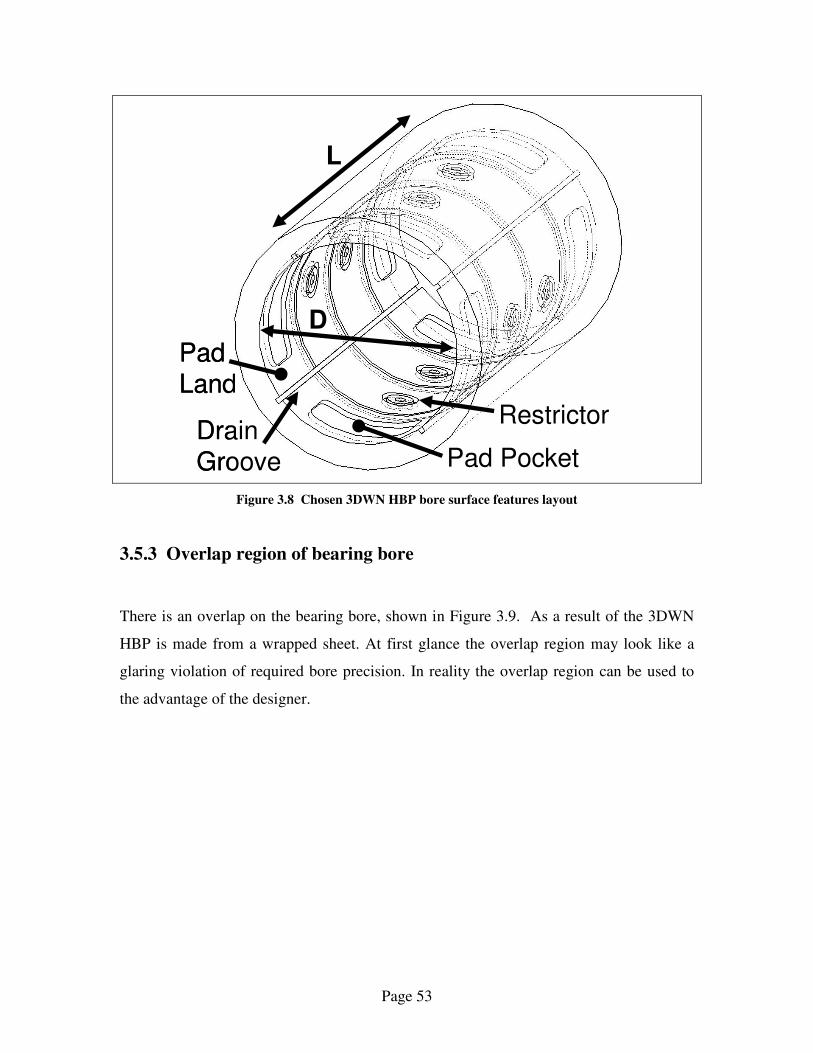
Figure 3.8 Chosen 3DWN HBP bore surface features layout
3.5.3 Overlap region of bearing bore
There is an overlap on the bearing bore, shown in Figure 3.9. As a result of the 3DWN
HBP is made from a wrapped sheet. At first glance the overlap region may look like a
glaring violation of required bore precision. In reality the overlap region can be used to
the advantage of the designer.
Page 54
w
w
w
w
Overlap Region
Overlap Gap
Drain Pocket
w
w
w
w
Overlap Region
Overlap Gap
Drain Pocket
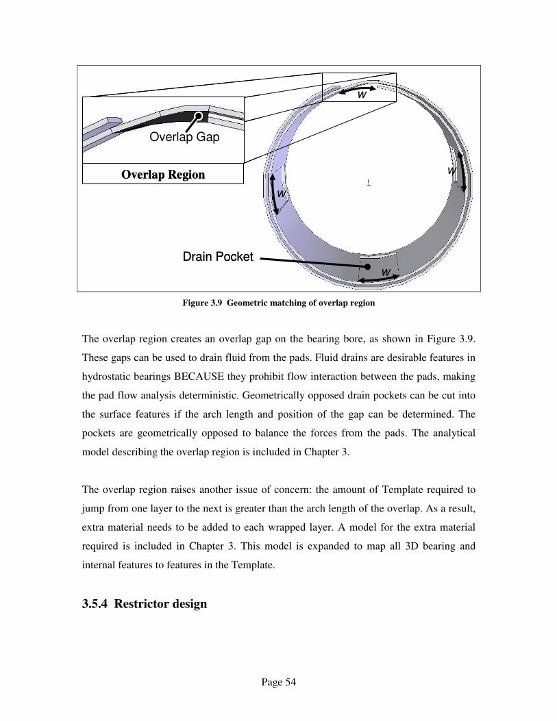
Figure 3.9 Geometric matching of overlap region
The overlap region creates an overlap gap on the bearing bore, as shown in Figure 3.9.
These gaps can be used to drain fluid from the pads. Fluid drains are desirable features in
hydrostatic bearings BECAUSE they prohibit flow interaction between the pads, making
the pad flow analysis deterministic. Geometrically opposed drain pockets can be cut into
the surface features if the arch length and position of the gap can be determined. The
pockets are geometrically opposed to balance the forces from the pads. The analytical
model describing the overlap region is included in Chapter 3.
The overlap region raises another issue of concern: the amount of Template required to
jump from one layer to the next is greater than the arch length of the overlap. As a result,
extra material needs to be added to each wrapped layer. A model for the extra material
required is included in Chapter 3. This model is expanded to map all 3D bearing and
internal features to features in the Template.
3.5.4 Restrictor design

Page 55
There is an inherent problem with incorporating annular restrictors into 3DWN
technology: a true annulus cannot be created, as this would create a physical separation
between two parts of the restrictor. As a result, it would not be possible to fabricate the
entire bearing template in one piece. A solution to this problem is shown in Figure 3.10.
2D Cut Template
Annulus
Connection
Fluid
Inlet
No Flow
2D Cut Template
Annulus
Connection
Fluid
Inlet
No Flow
Figure 3.10 Single feed, double annulus restrictor configuration
The design in Figure 3.10 is a modified annulus that keeps all features of the design
physically attached to the rest of the Template (the cuts are represented by gray areas).
The design in Figure 3.10 has the following desirable features that distinguish it from
restrictors designed by Slocum [15,22,23] and make it ideal for 3DWN technology:
1. Annulus connection: The annulus is supported by a web of material connected to
the surrounding Template. If this connection is sized correctly, it doesn’t impede
the radial flow from the annulus to center hole by allowing the flow from ends of
the annuls to converge at the center hole, shown in Figure 3.10.
2. Single source feeding: Placing the restrictors back to back permit both to be fed
from a single source. This feature allows a single annular internal fluid network to
feed all the restrictors. Making the feed network annular is important to limiting
pressure variation on the bore, which can cause bore bulge. Bore bulge is
quantified in Chapter 3.

Page 56
3.5.5 Full 3DWN HBP bore feature design
The 3DWN HBP bearing feature final design is shown in Figure 3.11. The axis of
symmetry in this figure corresponds to the center of the bearing, where an axial pad pair
meets. The pad bore surface features is repeated circumferentially 4 times around the
bore, creating a layout in the same configuration as shown in Figure 3.8.
s
rl
rl
l
l
l
l
m
Axis of Symmetry
m
Drain Pocket
Pad
Restrictor
m
m
s
rl
rl
l
l
l
l
m
Axis of Symmetry
m
Drain Pocket
Pad
Restrictor
m
m
Figure 3.11 3DWN self-compensated bearing pad bore surface features and geometric parameters
To simplify analysis of the bearing, the bore surface features in Figure 3.11 is designed to
be tunable with only one dimension: the pad width l. An analysis of bearing performance
is in included in Chapter 3. All other dimensions in Figure 3.11 were driven by
constraints and functional requirements placed on the bore surface features. An
explanation of the dimensions follows.
Page 57
• Drain pocket width s: This dimension is driven by the overlap region arch length
shown in Figure 3.9. Each pad has to have the same size drainage pocket to
balance with the other pads
• Minimum feature length m: The minimum feature size that can be cut into the
template is dependent on the type of cutting process used, the thickness and kind
of Template material, the flow of the adhesive during wrapping and bonding, and
ensuring flow is fully developed over the restrictor. A model for analyzing the
effect this dimension has on bearing performance is included in Chapter 3.
Minimizing this dimension is desirable, as more area on the pad can be used by
the pocket, which increases the load capacity and stiffness.
• Leakage radius rl: The leakage radius rl is used to calculate the leakage flow from
the restrictor. To make this calculation deterministic, the restrictor is equally
spaced from the vertical and horizontal drain pockets. The dimension rl is driven
by m and s.
3.6 Design of Internal Channels
The following functional requirements were outlined for the HBP internal networks.
1. 2D through cuts: All the features for internal channels have to be 2D and extend
through the entire thickness of the Template.
2. Low fluid resistance in the channels: The fluid restriction caused by the internal
networks should be negligible (three orders of magnitude less) compared to the
restriction of the pads and restrictors.
3. Feed channels: An internal network is required to supply the restrictors with
pressurized fluid.

Page 58
4. Cross-connection channels: Internal networks are required to connect the
restrictors with the pockets
5. Drain channels: Internal networks are required to remove fluid from the drain
channels.
Figure 3.12 shows the final design of the 3DWN HBP Template. Figure 3.12 shows the
Template cut into two sections since it is too long to be displayed as one piece. The
3DWN HBP has 13 wrapped layers, denoted by L1-L13 on the Template in Figure 3.12.
The successive subsections describe the design parameters used to satisfy the functional
requirements for the internal networks.
Bearing
topologyCross-connection channels
from restrictors to pads
Feed
channel
Drainage
channelsFluid
input
Fluid
output
L1 L2 L3 L4 L5 L6 L7
L8 L9 L10 L10 L11 L12 L13
Connection
holes
Bearing
topologyCross-connection channels
from restrictors to pads
Feed
channel
Drainage
channelsFluid
input
Fluid
output
L1 L2 L3 L4 L5 L6 L7
L8 L9 L10 L10 L11 L12 L13
Connection
holes
Figure 3.12 3DWN self-compensated bearing template
3.6.1 2D through-cut parameters
The same minimum dimension used in the bearing bore surface features of Figure 3.11,
m, was used as the internal channel width for all the HBP wrapped networks. Since the
internal networks are formed from thin sheets, the fluid resistance in the channels is

Page 59
dominated by the channel height (in the radial direction), hc, as long as the relationship in
Equation (3.3) is true.
tnhm cc ⋅=> (3.3)
Where nc is the number of layers in the channel and t is the thickness of each layer.
3.6.2 Design of HBP fluid networks for low resistance
The primary source of fluid resistance in the bearing should be from the restrictors and
the pads. An analysis of channel resistance as a function of channel width, m, is presented
in Chapter 3. To insure the channel resistance as a function of channel height is negligible
compared to the bearing resistance (three orders of magnitude difference), hc be at least
10X the bearing gap height.
3.6.3 Feed channel design
The feed channel supplies the restrictors with fluid. Fluid enters the bearing at a single
source, labeled in Figure 3.12 as “Fluid input,” and is distributed circumferentially
around the bearing. The feed channel is subjected to the highest pressure within the
bearing, and can thus be the main cause of bore bulge. A model for bore bulge is
presented in Chapter 3. To limit the effect of bulging, the feed channel is designed to be a
symmetric annulus around the bearing circumference. Only one feed ring is required, for
each restrictor pair (Figure 3.10) is fed by a single fluid input.
3.6.4 Cross-connection channel design
The cross-connection channels in the 3DWN HBP connect the restrictors with the pads
opposed 180o around the bearing bore. In Figure 3.12 the channels are arranged in a “fish
gill” configuration in order to:
Page 60
1. Minimize the distance the fluid has to travel between the restrictors and pads
2. Form a pattern that can be repeated through successive layers
3. Maximize the distance between the “Cross-connection channels” channels and the
“Connection holes” to reduce the possibility of leaks
3.6.5 Drainage channel design
The drainage channels collect fluid from the drain pockets and duct it to the outside of the
bearing. There are two channels, one for each set of 4 pads in the HBP bore surface
features. The drainage channels are located next to the feed channel to limit the amount
of material required for the Template.
3.7 Summary
This chapter describes the design decisions used in the 3DWN HBP and provides design
rules and metrics that can be applied to any 3DWN bearing design. The chapter begins
with the origins and conceptions of 3DWN technology. The remainder of the chapter
answers the following questions:
1. How can off-the-shelf parts be used to meet the precision requirements of fluid
film bearings? What level of precision is required from these parts?
2. How can conventional surface self-compensated bearing features to be cut as 2D
profiles and formed into a wrapped structure? How does the overlap region of the
wrapped Template affect the other features on the bearing surface?
3. How are internal wrapped fluid networks designed into a Template? How should
the channels be designed as to not affect bearing performance?

Page 61
CHAPTER
4 MODELING AND ANALYSIS
This chapter describes the modeling used in the 3DWN HBP. The model used to describe
a wrapped structure is derived in the first section. The wrapping model is then converted
into a transformation algorithm to convert points from a 3D cylindrical structure to 2D
coordinates on the Template. The second part of the chapter describes the fluid flow and
bearing performance models. The chapter concludes with an analysis of the sensitivity of
manufacturing errors on bearing performance, as well as other sensitivities to be
considered when designing the 3DWN HBP.
4.1 Wrapping model 4.1.1 Describing a wrapped structure
When the Template is wrapped, it breaks contact with the mandrel in the overlap zone
between the first and second layer, as shown in Figure 4.1. The overlap zone is important
because l is longer than s, meaning the overall length of the layer will be longer than the
circumference of the mandrel.

Page 62
l
xo
so
t
ro θo
θo
yo
F
Tangent
Mandrel
Template
Figure 4.1 Diagram of overlap region of layer one and two
The overlap region is modeled as a cantilevered beam, as shown in Figure 4.1. The base
of the beam has a zero slope condition and the end of the beam is tangent with the
mandrel. The assumptions made in the wrapping model are as follows:
1) Although 3DWN bearings are wrapped under tension, only the vertical
component of the tensile force is used in the analysis as stretching can be
considered negligible. This simplification is justified in a later section.
2) Wide beam (w > l) stiffening is also neglected as it does not affect the beam shape
for a fixed displacement [24].
l
xo
so
t
ro θo
θo
yo
F
Tangent
Mandrel
Template
lo
xo
so
t
ro θo
θo
yo
F
Tangent
Mandrel
Template

Page 63
3) Bending stress does not exceed the yield stress (σys). Elastic deflection is insured
if Equation (4.1) is true.
ys
or
Etσ<
2 (4.1)
4) Changes in moment as a result of geometric changes are negligible with
deflection (ie lo ~ xo).
In Figure 4.1 there are two knowns (ro, t) and six unknowns (yo,F,lo,so,xo,θo). Geometric
conditions are used to write Equations (4.2)-(4.4) and bending beam theory for Equations
(4.5) and (4.6).
)cos1( ooo rty θ−+= (4.2)
ooo rx θsin= (4.3)
ooo rs θ= (4.4)
EI
Fly o
o3
3
= (4.5)
EI
Floo
2
2
=θ (4.6)
Where E is the modulus of elasticity and I is the moment of inertia.
Equation (3.6) is found by using Equation (4.7), which is taken from Bernoulli-Euler
beam theory.

Page 64
dl
d
EI
M θ= (4.7)
Equation (4.7) is used to obtain the horizontal deflection. Using the geometry of a
differential beam element shown in Figure 4.2, Equation (4.8) can be written.
xo
l
dθdl
dy
y
x
dx
xo
l
dθdl
dy
y
x
dx
Figure 4.2 Model used for x-displacement of cantilevered beam
θcos
dxdl = (4.8)
Combining Equations (4.8) and (4.7), and substituting )( xlFM o −= for the moment in
the beam yields Equation (4.9).
θθ
cos)(
dx
d
EI
xlF o =−
(4.9)
Integrating over the intervals shown in Figure 4.1 yields Equation (4.10). Evaluating
Equation (4.10) results in a quadratic polynomial of xo with one possible root, shown in
Equation (4.11).

Page 65
( ) ∫∫ =−oo
dF
EIdxxl
x
o
θ
θθ00
cos (4.10)
ooooF
EIllx θsin
22−−=
(4.11)
Combining Equations (4.2)-(4.6) and (4.11) results in Equation (4.12). Equation (3.12)
relates the known parameters of ro and t to the arc length of the overlap region, so. This
equation can be used for any layer of the wrapped structure by changing the variables
from first layer values (subscript o) to values of the local layer (subscript i). Values of s
have to be calculated numerically since Equation (4.12) cannot be simplified to a closed-
form solution.
o
oo
o
o
i
o
o
oo
o
o
r
sr
r
s
s
r
r
srt
s
rsinsin11cos1
2
30 −
−−
−+=
(4.12)
4.1.2 3D to 2D coordinate transformation
For Equation (4.12) to be useful, it has to be incorporated into an algorithm to transform
coordinates in a 3D cylindrical structure to 2D coordinates on the Template, as shown by
Figure 4.3.
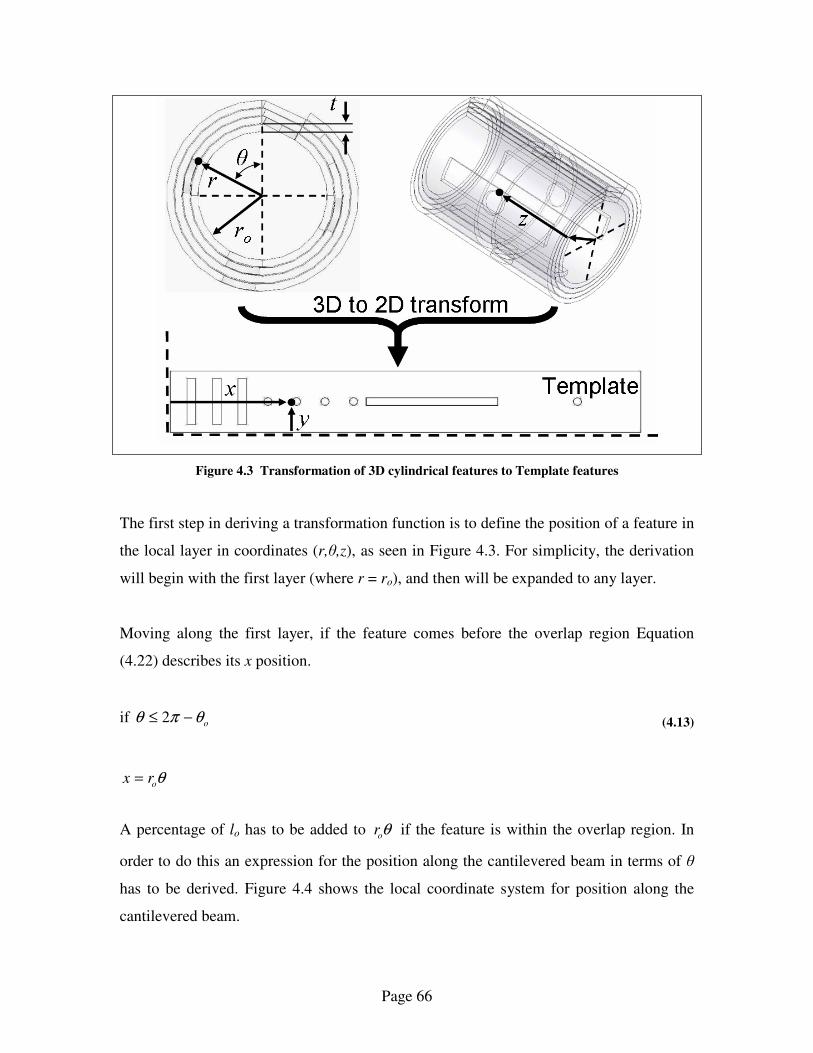
Page 66
Figure 4.3 Transformation of 3D cylindrical features to Template features
The first step in deriving a transformation function is to define the position of a feature in
the local layer in coordinates (r,θ,z), as seen in Figure 4.3. For simplicity, the derivation
will begin with the first layer (where r = ro), and then will be expanded to any layer.
Moving along the first layer, if the feature comes before the overlap region Equation
(4.22) describes its x position.
if oθπθ −≤ 2
θorx =
(4.13)
A percentage of lo has to be added to θor if the feature is within the overlap region. In
order to do this an expression for the position along the cantilevered beam in terms of θ
has to be derived. Figure 4.4 shows the local coordinate system for position along the
cantilevered beam.

Page 67
Mandrel center
l’lo
θ’
θo
Figure 4.4 Local coordinate system for position along cantilevered beam
Equation (4.7) is used again to describe the deflection of the beam. Substituting the
moment with )( llFM o −= results in Equation (4.14).
dl
d
EI
llF o θ=
− )( (4.14)
Integrating over the range shown in Figure 4.4 results in Equation (4.15).
θ ′=
′−′
EI
lllF o
2
2
(4.15)
Equation (4.15) is related back to the coordinate system in Figure 4.3 by substituting for
2π - θ = θ’, resulting in Equation (4.16).

Page 68
θπ −=
′−′
22
2
EI
lllF o
(4.16)
Combining Equation (4.16) with Equations (4.4) and (4.6) produces a polynomial with
one possible root that is shown in Equation (4.17).
( )
−−−=′
o
oo
s
rll
θπ211
(4.17)
The x coordinate within the overlap region, given by Equation (4.18), is found by
summing the length of material in contact with the mandrel and the difference between lo
and l’.
if oθπθ −> 2
( )
o
oooo
s
rlsrx
θππ
−−+−=
212
(4.18)
Combining Equations (4.2) and (4.4)-(4.6) creates an expression for lo, given by Equation
(4.19).
−+=
o
oooo
r
srrt
s
rl cos
2
3
0
0 (4.19)
Equation (4.19) can be used in any layer by changing the variables to values in that layer
(subscript change from 0 to n, where n is the number of the local layer). The local layer
number is found using Equation (4.20)
−=
t
rrn oint (4.20)
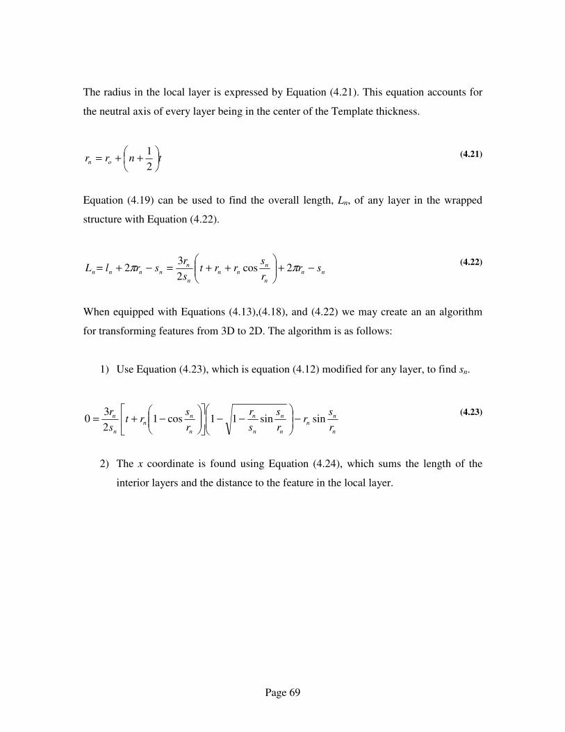
Page 69
The radius in the local layer is expressed by Equation (4.21). This equation accounts for
the neutral axis of every layer being in the center of the Template thickness.
tnrr on
++=
2
1 (4.21)
Equation (4.19) can be used to find the overall length, Ln, of any layer in the wrapped
structure with Equation (4.22).
nn
n
nnn
n
nnnnn sr
r
srrt
s
rsrlL −+
++=−+= ππ 2cos
2
32
(4.22)
When equipped with Equations (4.13),(4.18), and (4.22) we may create an an algorithm
for transforming features from 3D to 2D. The algorithm is as follows:
1) Use Equation (4.23), which is equation (4.12) modified for any layer, to find sn.
n
nn
n
n
n
n
n
nn
n
n
r
sr
r
s
s
r
r
srt
s
rsinsin11cos1
2
30 −
−−
−+=
(4.23)
2) The x coordinate is found using Equation (4.24), which sums the length of the
interior layers and the distance to the feature in the local layer.

Page 70
if 0=n
=x
θ
+ tro
2
1if
tr
s
o
o
2
12
+−≤ πθ
o
o
oos
tr
lstr
+−
−+−
+
2
1)2(
12
12
θππ if
tr
s
o
o
2
12
+−> πθ
if 0>n
∑−
=
+=1
0
n
i
iLx
θ
++ tnro
2
1if
tnr
s
o
o
++
−≤
2
12πθ
o
o
oos
tnr
lstnr
++−
−+−
++
2
1)2(
12
12
θπ
π if
tnr
s
o
o
++
−>
2
12πθ
(4.24)
3) The z coordinate simply becomes the y coordinate, shown in Equation (4.25).
zy = (4.25)
4.2 Modeling bearing performance 4.2.1 Fluid resistance modeling
The bore surface features and modeling used for the HBP is based on surface self-
compensated hydrostatic bearing theory from Slocum [1]. Figure 4.5 shows the fluid flow
of one restrictor-pad set. The HBP bore surface features is composed of 4 restrictor-pad
sets placed back to back (restrictors fed by same source), arranged π/2 radians apart
around the bore, as was shown in Chapter 2.

Page 71
a
b
Fluid flow
φ
l
rp
Leakage flowPad flow
Restrictor flow
rl
rh
rarr
a
b
Fluid flow
φ
l
rp
Leakage flowPad flow
Restrictor flow
rl
rh
rarr
Figure 4.5 Flow over bearing bore surface features
To review from Chapter 1, the bearing self-compensates because each restrictor is
connected to the pad located π radians around the bore. When the shaft is displaced
downward the restrictor resistance changes such that pressure is increased under the shaft
and decreased above the shaft. The same fluid circuit shown in Chapter 1, shown again in
Figure 4.1, is used to model the HBP.
Figure 4.6 Fluid circuit of one set of opposed pads in the HBP
Ps
RUR
RLPRLR
RUP
RLL
RUL
PA
Ps
RUR
RLPRLR
RUP
RLL
RUL
PA
Ps
RUR
RLPRLR
RUP
RLL
RUL
PA
Ps
RUR
RLPRLR
RUP
RLL
RUL
PA

Page 72
The flow through the bearing is modeled as fully-developed, viscous flow. Using the
same method of evaluating resistance presented in Chapter 1, The Navier-Stokes
equations reduce such that the nominal resistances are as follows. The derivation of these
resistances can be found in any common fluids textbook [25].
Equation (4.26) for the upper restrictor resistance, RUR, and lower restrictor resistance,
RLR.
3
ln6
h
r
r
RRh
a
LRURπ
µ
==
(4.26)
Equation (4.27) for the upper pad resistance, RUP, and lower pad resistance, RLP.
( )
++
+==
p
p
LPUP
r
lr
h
l
hbaRR
ln66
133
µ
π
µ
(4.27)
Equation (4.28) for the upper leakage resistance RUL, , and lower leakage resistance, RLL.
)2(
2ln6
3 ϕπ
π
π
µ
−
==h
r
r
RRr
l
LRUR
(4.28)
The factor )2(
2
ϕπ
π
− in Equation (4.28) accounts for the no-flow zone. This zone occurs
since there is no pressure differential to drive the flow between restrictors.
4.2.2 Resistance ratio

Page 73
The resistance ratio between the restrictors and pads is defined by Equation (4.29)
UP
LR
LP
UR
R
R
R
R==γ (4.29)
Slocum [1] suggests the resistance ratio should be between 3 and 4 for uniform stiffness.
The resistance ratio chosen for the HBP was 3.25. This ratio was met by tuning the
dimension l on the bearing pad.
4.2.3 Derivation of effective pad area
The pressure profile over each pad is trapezoidal in shape, as shown in Figure 4.7.
Restrictor
a+2rp
ll
b+2rp
Pp
Restrictor
a+2rp
ll
b+2rp
Pp
Zone 2
Zone 3
Zone 1
Figure 4.7 Pressure profile over bearing pad
The purpose of deriving an effective area is so the resultant force from the pad can be in
the form of Equation (4.30).
effp APF ⋅= (4.30)
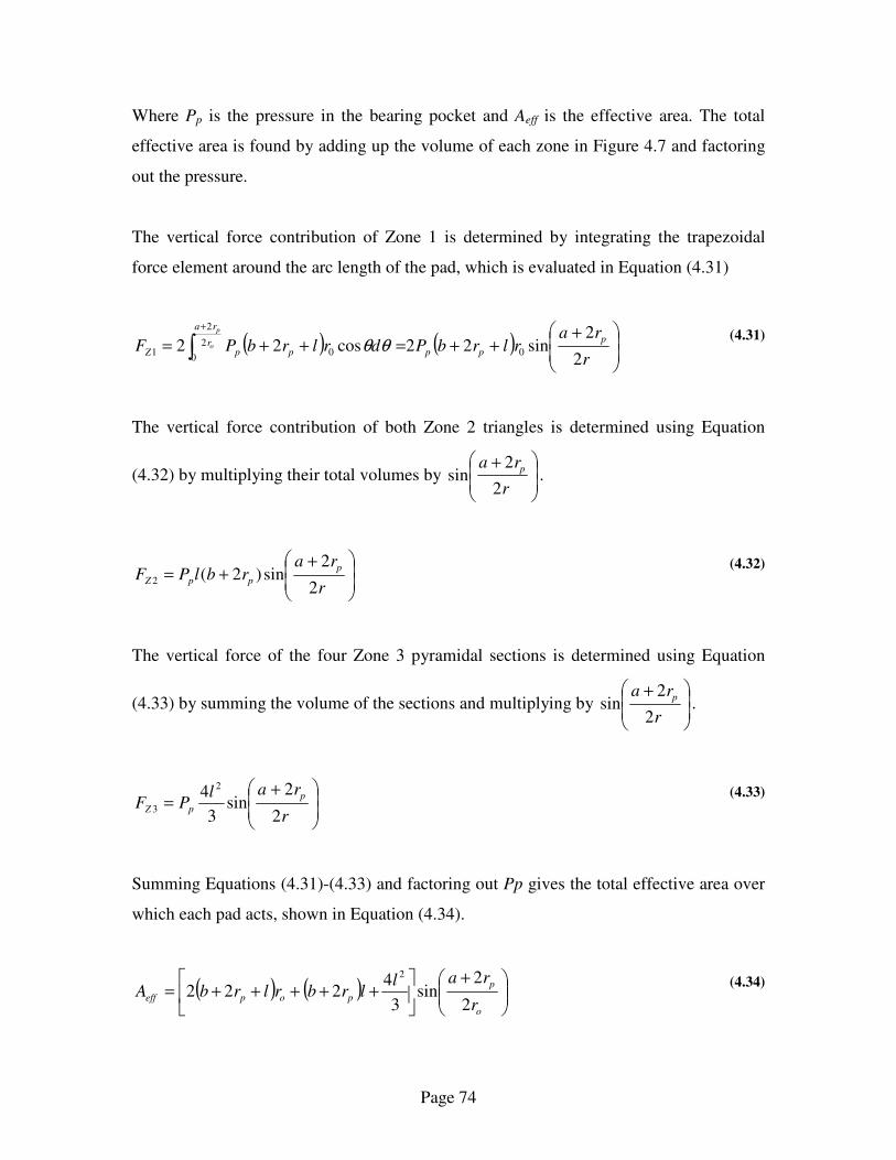
Page 74
Where Pp is the pressure in the bearing pocket and Aeff is the effective area. The total
effective area is found by adding up the volume of each zone in Figure 4.7 and factoring
out the pressure.
The vertical force contribution of Zone 1 is determined by integrating the trapezoidal
force element around the arc length of the pad, which is evaluated in Equation (4.31)
( ) ( )
+++=++= ∫
+
r
rarlrbPdrlrbPF
p
ppr
ra
ppZo
p
2
2sin22cos22 0
2
2
001 θθ
(4.31)
The vertical force contribution of both Zone 2 triangles is determined using Equation
(4.32) by multiplying their total volumes by
+
r
ra p
2
2sin .
++=
r
rarblPF
p
ppZ2
2sin)2(2
(4.32)
The vertical force of the four Zone 3 pyramidal sections is determined using Equation
(4.33) by summing the volume of the sections and multiplying by
+
r
ra p
2
2sin .
+=
r
ralPF
p
pZ2
2sin
3
4 2
3 (4.33)
Summing Equations (4.31)-(4.33) and factoring out Pp gives the total effective area over
which each pad acts, shown in Equation (4.34).
( ) ( )
+
+++++=
o
p
popeffr
rallrbrlrbA
2
2sin
3
4222
2
(4.34)

Page 75
4.2.4 Derivation of bearing stiffness
To develop a stiffness model the bearing is oriented such that four pads are vertical and
four are horizontal, as shown in Figure 4.1. Only the vertically oriented pads are loaded;
shaft deflections are small enough to assume the horizontal pads contribute zero stiffness
in the vertical direction.
y
xz
Shaft
Bearing
Pad stiffness
Load
y
xz
Shaft
Bearing
Pad stiffness
Load
Figure 4.8 Pad stiffness configuration of HBP (gap greatly exaggerated)
The voltage divider rule (P=QR for fluid circuits) can be applied to find the pressure
difference between the pads by using the circuit in Figure 4.6 and Equations (4.26) and
(4.27). Each resistance in the circuit is a function of the gap height and will change with
displacement of the shaft. Multiplying the pressure difference between the upper and
lower pads by the effective area gives the resultant force on the shaft. Equation (4.35)
gives the force as a function of shaft displacement, δ.
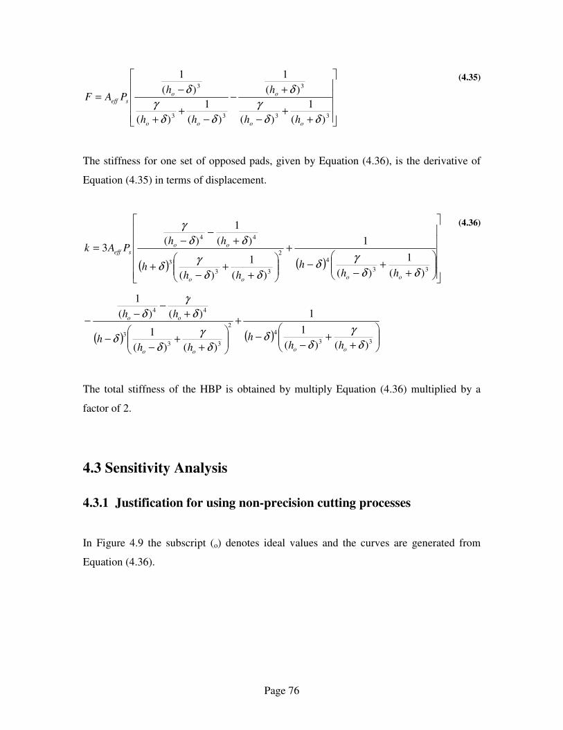
Page 76
++
−
+−
−+
+
−=
33
3
33
3
)(
1
)(
)(
1
)(
1
)(
)(
1
δδ
γ
δ
δδ
γ
δ
oo
o
oo
o
seff
hh
h
hh
hPAF
(4.35)
The stiffness for one set of opposed pads, given by Equation (4.36), is the derivative of
Equation (4.35) in terms of displacement.
( ) ( )
++
−−
+
++
−+
+−
−=
33
42
33
3
44
)(
1
)(
1
)(
1
)(
)(
1
)(3
δδ
γδ
δδ
γδ
δδ
γ
oooo
ooseff
hhh
hhh
hhPAk
( ) ( )
++
−−
+
++
−−
+−
−−
33
42
33
3
44
)()(
1
1
)()(
1
)()(
1
δ
γ
δδ
δ
γ
δδ
δ
γ
δ
oooo
oo
hhh
hhh
hh
(4.36)
The total stiffness of the HBP is obtained by multiply Equation (4.36) multiplied by a
factor of 2.
4.3 Sensitivity Analysis
4.3.1 Justification for using non-precision cutting processes
In Figure 4.9 the subscript (o) denotes ideal values and the curves are generated from
Equation (4.36).

Page 77
0.8 0.85 0.9 0.95 1 1.05 1.1 1.15
0.6
0.8
1
1.2
1.4
Expected εl – from
through-cutting
Expected εh – from mandrel
( )
l/lo, h/ho
k/ko
k(l)
k(h)(
Figure 4.9 Sensitivity of the HBP stiffness to manufacturing errors for h/R = .002, h/l = 0.011
The principle errors that affect bearing stiffness (k) are:
1) Errors in the fluid film height (εh), caused by manufacturing errors in the mandrel
or the shaft used in the bearing
2) errors in the dimensions of the bore surface features (εl), caused by errors in the
through-cutting process used for the Template.
Tolerances of the mandrel radius are typically much better (10X) than the tolerances of
the Template. The stiffness is much more sensitive to errors in the mandrels since
hl
hl εε<< and
hk
1∝ , whereas lk ∝ . This means a non-precise through-cutting process
(like laser or waterjet) can be used to manufacture the Template, as the performance of
the bearing will be dependent on the precision of the off-the-shelf parts and not the
Template.

Page 78
4.3.2 Sensitivity of performance to internal channel errors
Internal channel resistance, Rc, being significant compared to the resistance of the bearing
features, Rb, can cause a negative effect on bearing performance. Errors in Template
thickness and mandrel radius cause misalignment of internal features, as shown in Figure
4.10, which decrease the effective channel width and can choke bearing fluid flow.
wo
w
Layer n+1
Layer n
Flow
wo
w
Layer n+1
Layer n
Flow
Figure 4.10 Channel constriction as a result of internal feature misalignment
Using Equation (4.24), values of m were calculated for different ideal widths (mo) by
varying mandrel radius (r) and the Template thickness (t) over the expected error range of
the off-the-shelf parts used for the HBP. The comparison between resistances was made
using the approximations in Equations (4.37) and (4.38). The results of this analysis are
displayed in Figure 4.11.
3
1~
o
bh
R (4.37)
3
1~
mRc (4.38)

Page 79
0.9
99
75
0.9
99
85
0.9
99
95
1.0
00
05
1.0
00
15
0.8
00
00
0.8
88
89
0.9
77
78
1.0
66
67
1.1
55
56
7.94E-09
7.96E-09
7.98E-09
8E-09
8.02E-09
8.04E-09
8.06E-09
8.08E-09
8.1E-09
8.12E-09
r/r o t/t o
m o /h o = 500
R c /R b
0.9
99
75
0.9
998
5
0.9
999
5
1.0
00
05
1.0
00
15
0.8
00
00
0.8
88
89
0.9
777
8
1.0
66
67
1.1
55
56
0.0000074
0.0000076
0.0000078
0.000008
0.0000082
0.0000084
0.0000086
0.0000088
0.000009
0.0000092
r/r o t/t o
m o /h o = 50
R c /R b
0.9
99
75
0.9
99
85
0.9
99
95
1.0
00
05
1.0
00
15
0.8
00
00
0.8
88
89
0.9
77
78
1.0
66
67
1.1
55
56
0
0.005
0.01
0.015
0.02
0.025
0.03
0.035
0.04
0.045
r/r o t/t o
m o /h o = 5
R c /R b
Figure 4.11 Internal channel resistance sensitivity to expected error range of t and R for t/R = 0.01

Page 80
The trends in Figure 4.11 were used to choose a channel ratio of mo/ho = 50 for the HBP,
which corresponds to mo = 2.54mm. This value of mo insures manufacturing errors will
not affect bearing performance and also gives a buffer for glue squeeze into the channels.
It is important to note that angular misalignment (e.g the Template not being
perpendicular to the mandrel, resulting in spiraling error during rolling) was not
considered in the sensitivity analysis. This decision was made because angular
misalignment is an error that could be actively corrected for during the rolling process,
whereas manufacturing errors are inherent to the precision parts.
4.3.3 Justification for neglecting tension in the wrapping model
As was mentioned in the beginning of this chapter, stretching effects due to tension were
neglected from the wrapping model. This assumption was validated in two ways:
1) The strain over the entire Template was calculated to be on the same order as the
manufacturing errors used to make the through-cuts.
2) An FEA analysis was conducted on the section of Template in the overlap region
to determine if tension would change the beam shape and resultant length, as
shown in Figure 4.12. The maximum calculated change in length over the
cantilevered beam was 0.01%, which can be regarded as negligible.
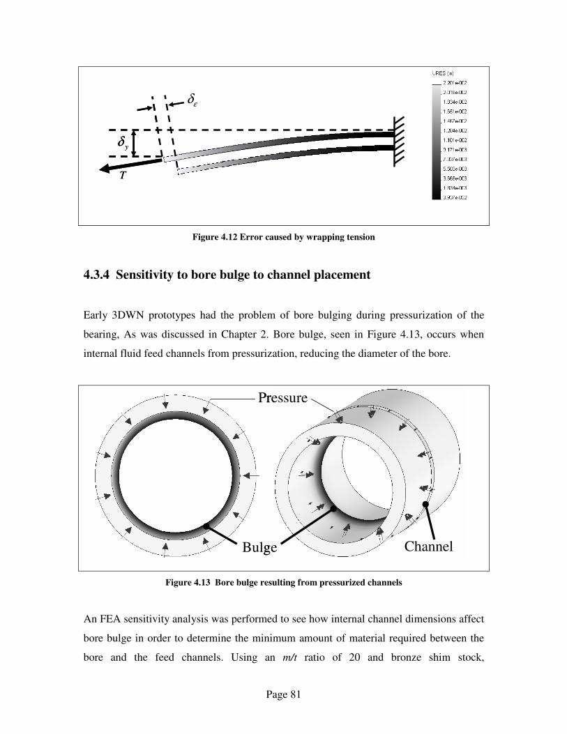
Page 81
yδ
T
εδ
yδ
T
εδ
Figure 4.12 Error caused by wrapping tension
4.3.4 Sensitivity to bore bulge to channel placement
Early 3DWN prototypes had the problem of bore bulging during pressurization of the
bearing, As was discussed in Chapter 2. Bore bulge, seen in Figure 4.13, occurs when
internal fluid feed channels from pressurization, reducing the diameter of the bore.
Pressure
ChannelBulge
Pressure
ChannelBulge
Figure 4.13 Bore bulge resulting from pressurized channels
An FEA sensitivity analysis was performed to see how internal channel dimensions affect
bore bulge in order to determine the minimum amount of material required between the
bore and the feed channels. Using an m/t ratio of 20 and bronze shim stock,

Page 82
corresponding to one layer of the Template, the bore bulge was three orders of magnitude
smaller than the bearing gap, making its affect on bearing performance insignificant.
4.3.5 Appropriate wrapping tension to compress Template deformities
Deformities in the Template were observed preventing contact between the layers in early
prototypes. To compress such deformities an appropriate amount of wrapping tension had
to be determined. The Template thickness was determined by using a level of constant
tension that could easily be produced in a lab. The tension used in wrapping was 90 N (20
lbs), which was produced by four 22.25 N (5 lbs) barbell plates. The satisfactory amount
of vertical deflection of one Template layer was chosen to be 254 µm, a value which is on
the same order as the thickness. Further detail on the wrapping process is described
Chapter 4.
The model used for the FEA tension analysis is shown in Figure 4.14. The pressure
applied to the top surface of the beam in Figure 4.14 was determined by using a thin-wall
pressure vessel model. If adjacent layers are permitted to slide against one another, which
liquid-state glue permits, then the tension pulling on π radians of the Template will be
reacted by a pressure analogous to that on half of a cylindrical pressure vessel.
Pressure
T T
δy
Template
Pressure
T T
δy
Template
Figure 4.14 Deflection of Template due to tension

Page 83
FEA results from the loading condition in Figure 4.14 are shown in Figure 4.15. All
analyzed thicknesses meet the desired deflection. The Template thickness was chosen to
be 127 µm, which corresponds to the thinnest bronze shim stock commonly available, to
obtain the maximum possible deflection.
0
1000
2000
3000
4000
5000
6000
254 203.2 177.8 127 101.6
t (microns)
δy
(mic
rons)
Figure 4.15 FEA Results from deformity deflection under tension
4.4 Summary This chapter the modeling and analysis used in designing the 3DWN HBP. A model to
transform coordinates in a 3D structure to a 2D Template is presented. Conventional self-
compensated hydrostatic bearing theory is used to model the HBP performance. The
sensitivity of bearing performance to manufacturing errors is explored. The sensitivity
analysis concludes that bearing stiffness sensitivity is dominated by defects in the
precision ground mandrel and not errors in the cutting process. The chapter concludes
with verifications of simplifications made in the wrapping model and calculations of
design and manufacturing parameters that ensure proper bearing performance.

Page 84
CHAPTER
5 MANUFACTURING A 3DWN HBP
This chapter describes the methods used in manufacturing a 3DWN HBP. The chapter
begins with a review of failed strategies of adhering wrapped layers together. The
remainder of the chapter describes the manufacturing processes used in making the final
HBP. The manufacturing processes are broken into three sections: 1) how the Template
was cut, 2) how the Template was wrapped, and 3) how the Template was packaged into
a housing.
5.1 Failed attempts at adhering wrapped layers Table 5.1 summarizes the methods attempted and the causes of failure in trying to adhere
3DWN wrapped layers. A concern in early HBPs was that a liquid adhesive would clog
the internal channels. Another concern was adhesive strength; early 3DWN aerostatic
prototypes were made with double-stick tape, which was not strong enough to prevent
bore bulge. The methods of adhesion stated in Table 5.1 were all chosen for high bond
strength and minimized flow into the internal channels.
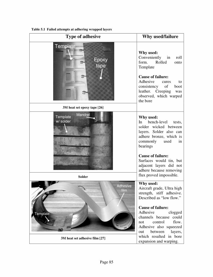
Page 85
Table 5.1 Failed attempts at adhering wrapped layers
Type of adhesive Why used/failure
Template
Epoxy
tape
3M heat set epoxy tape [26]
Why used: Conveniently in roll form. Rolled onto Template Cause of failure: Adhesive cures to consistency of boot leather. Creeping was observed, which warped the bore
Template
w/ solder
Mandrel
Solder
Why used: In bench-level tests, solder wicked between layers. Solder also can adhere bronze, which is commonly used in bearings Cause of failure: Surfaces would tin, but adjacent layers did not adhere because removing flux proved impossible.
Adhesive
film
Template
3M heat set adhesive film [27]
Why used: Aircraft grade, Ultra high strength, stiff adhesive. Described as “low flow.” Cause of failure: Adhesive clogged channels because could not control flow. Adhesive also squeezed out between layers, which resulted in bore expansion and warping.
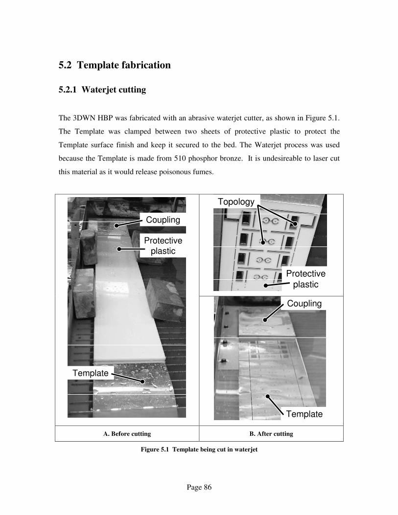
Page 86
5.2 Template fabrication
5.2.1 Waterjet cutting
The 3DWN HBP was fabricated with an abrasive waterjet cutter, as shown in Figure 5.1.
The Template was clamped between two sheets of protective plastic to protect the
Template surface finish and keep it secured to the bed. The Waterjet process was used
because the Template is made from 510 phosphor bronze. It is undesireable to laser cut
this material as it would release poisonous fumes.
Protective
plastic
Topology
Coupling
Protective plastic
Template
Coupling
Template
A. Before cutting B. After cutting
Figure 5.1 Template being cut in waterjet

Page 87
5.2.2 Fixturing of Template within waterjet
The Template for the HBP had to be cut in segments because it was longer than the
waterjet bed. A kinematic fixturing system, shown in Figure 5.2, was incorporated into
the Template to maintain alignment between segments. Each coupling feature has a
single point contact with a pin on the 3-pin plate and is pre-loaded with a flexure. The 3-
pin-plate was cut in the same waterjet as the Template and positioned at the same zero to
preserve the alignment of the machine axes.
Clamping plateTemplate
Coupling feature
Perforation
Preload
Flexure3-pin plate
Clamping plateTemplate
Coupling feature
Perforation
Preload
Flexure3-pin plate
Figure 5.2 Kinematic fixture for waterjet cutting, waterjet cutting setup
The sides of the Template, which include the coupling features, are not necessary for
bearing function and are designed to be easily removed after fabrication. The perforations
incorporated into the Template, shown in Figure 5.2, allow the coupling features to be
snapped off.
5.3 Template wrapping 5.3.1 Rolling jig

Page 88
The rolling jig shown in Figure 5.3 was used to wrap the HBP. All of the components in
the jig were made from Delrin and cut on a waterjet. Delrin was the chosen because it has
a low coefficient of friction against steel, allowing the mandrel to turn easily. Delrin is
also commonly used for flexures, making it a good choice for the friction break.
Mandrel
Crank
Bearing blocks
Friction clamp
Constraining clamp
Figure 5.3 3DWN bearing rolling jig
The rolling jig was mounted to an optical table. The constraining clamps constrain the
mandrel from moving axially, and allow the crank to be positioned so it clears the table.
The friction break allows tension to be maintained on the Template during pauses in
wrapping.
5.3.2 Alignment of Template to mandrel
Figure 5.4 shows how the Template was mounted to the rolling jig, and how the rolling
jig was mounted to an optical table. Before the HBP Template was mounted all burrs

Page 89
were removed. Surfaces to accept adhesive were prepared by light sanding and cleaning
with alcohol.
Weights
Tension
distributor
Template
Level
Mandrel
Rolling crank
Tension
balancer
Figure 5.4 Template mounted on rolling jig
The Template was aligned on the rolling jig by using the following process:
1) The sacrificial tabs at the beginning of the Template were affixed to the mandrel
with hose clamps.

Page 90
2) Weights were hung at the end of the Template to provide the calculated required
wrapping tension.
3) The hose clamps were tapped outwards to pull the leading edge of the Template
flush to the mandrel.
4) The sine error was measured over the horizontal Template length and adjusting
with the Tension distributor.
5) The hose clamps were slowly loosened until the Template was level.
The use of a level to measure tension over the Template was realized after observing the
relationship in Equation (5.1).
dw
dT=α (5.1)
Where α is the roll angle across the width of the Template, w is the template width, and T
is the applied tension.
5.3.3 Adhesion of wrapped layers
Superglue gel was used to adhere adjacent wrapped layers within the 3DWN HBP. Gel
over liquid super glue was chosen because it doesn’t cure as quickly and doesn’t wick.
The mandrel was coated with a light oil to prohibit the superglue from adhering. The
Template surface was cleaned before the glue was applied using alcohol to remove any
oil, as shown in Figure 5.5A.

Page 91
Hose clamp
Alcohol
Template
Mandrel
Hose clamp
Super glue
Template
Mandrel
A. Cleaning surface with alcohol B. Applying superglue gel
Figure 5.5 Adhering adjacent layers within the HBP
Adhering all surfaces in the first layer is important because the bore surface features have
to conform to the mandrel. Figure 5.5B shows how the superglue was applied to the first
layer. In the first layer, excess glue that spilled into the bearing features was removed
after the mandrel was taken out of the bearing. Glue within the channels was removed by
dabbing it out through the cutouts in the second layer. Glue was applied to layers beyond
the first in such a way to limit spreading into the channels. As a result, closely located
features in the Template could not be sealed from one another.
5.4 Packaging the Template in a housing 5.4.1 Joining Template and housing
A housing is required for the wrapped Template because it provides a connection to a
pressurized fluid source and rigidity for mounting. The first step in packaging the
Template was to affix it in the center of the housing. The Template was glued to two
concentric centering shims, as shown in Figure 5.6. The shims were then glued to the
housing.

Page 92
Aluminum sleeve
Wrapped
Template
Centering shims
Aluminum sleeve
Wrapped
Template
Centering shims
Figure 5.6 Centering of Template within housing
5.4.2 Prepping the HBP for casting
The wrapped Template has openings for fluid input and output. The methods used in
preventing casting epoxy from entering these openings are shown in Figure 5.7. The
inlets and outlets on the Template were covered with electrical tape, shown in Figure
5.7A. Then the openings in the housing were plugged with grease packed foam, shown in
Figure 5.7B. The plugs, when preloaded against the outer surface of the wrapped
Template, prohibit epoxy from building up over the electrical tape and filling the
openings in the housing.
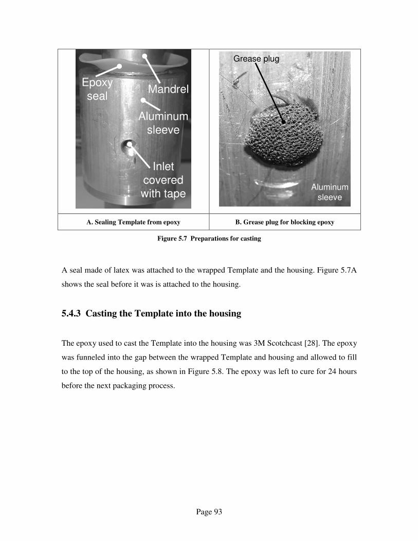
Page 93
Epoxy
sealMandrel
Aluminum sleeve
Inlet
covered with tape
Grease plug
Aluminum
sleeve
A. Sealing Template from epoxy B. Grease plug for blocking epoxy
Figure 5.7 Preparations for casting
A seal made of latex was attached to the wrapped Template and the housing. Figure 5.7A
shows the seal before it was is attached to the housing.
5.4.3 Casting the Template into the housing
The epoxy used to cast the Template into the housing was 3M Scotchcast [28]. The epoxy
was funneled into the gap between the wrapped Template and housing and allowed to fill
to the top of the housing, as shown in Figure 5.8. The epoxy was left to cure for 24 hours
before the next packaging process.

Page 94
Mandrel
Epoxy
Aluminum sleeve
Figure 5.8 Wrapped Template cast in housing
5.4.4 Finishing procedures
The grease plugs were removed after the epoxy dried. Notice in Figure 5.9 how the
drainage plugs in the wrapped template are visible; the grease plugs and electrical tape
prevented epoxy from reaching the drainage ports in the Template.
Drainage ports after cleaning
Aluminum sleeve
Figure 5.9 Drainage ports with grease plugs removed

Page 95
The mandrel was removed with an arbor press. The final process in packaging the HBP
was to remove the excess superglue in the bore surface features, shown in Figure 5.10.
The glue was carefully cut out of the bore using a hobby knife.
Template
topology
Residual super glue
Figure 5.10 Residual super glue to be removed from bearing bore surface features
5.5 Summary This chapter explains how the 3DWN HBP was manufactured. Unsuccessful attempts
adhering the wrapped layers are presented in the first section. The remainder of the
chapter describes in three sections the manufacturing processes used for the final HBP.
The first section describes how the Template was cut in segments using a waterjet. The
second section describes how the Template was wrapped and adhered. The third section
describes how the bearing was finished and packaged into a housing.

Page 96
CHAPTER
6 EXPERIMENTAL VERIFICATION
The purpose of this chapter is to verify the feasibility of 3DWN technology by comparing
the HBP performance to the models developed in Chapter 3 and determining if the bore
precision is within the metrics outlined in Chapter 2. This chapter begins with a
description of the experimental setups used to measure bearing stiffness and bore
geometry. Results from these tests are presented and compared against theoretically
predicted and ideal values. A discussion and interpretation of the results and sources of
error is included. The financial benefits of 3DWN technology are exhibited in a cost
comparison between the HBP and a babbitted, self-compensated bearing of the same size
and surface feature layout.
6.1 Experimental setup 6.5.1 Parameters of the 3DWN HBP used in experimentation
The parameters of the 3DWN HBP used for experimentation are shown in Table 6.1. The
methods behind generating and outlining the parameters in this bearing are described in
Chapters 2-4.
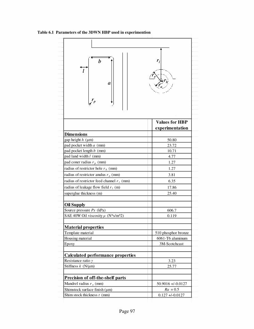
Page 97
Table 6.1 Parameters of the 3DWN HBP used in experimention
Values for HBP
experimentation
Dimensionsgap height h (µm) 50.80
pad pocket width a (mm) 23.72
pad pocket length b (mm) 10.71
pad land width l (mm) 4.77
pad coner radius r p (mm) 1.27
radius of restrictor hole r h (mm) 1.27
radius of restrictor anulus r a (mm) 3.81
radius of restrictor feed channel r r (mm) 6.35
radius of leakage flow field r l (m) 17.86
superglue thickness (m) 25.40
Oil SupplySource pressure Ps (kPa) 606.7
SAE 40W Oil viscosity µ (N*s/m^2) 0.119
Material propertiesTemplate material 510 phosphor bronze
Housing material 6061-T6 aluminum
Epoxy 3M-Scotchcast
Calculated performance propertiesResistance ratio γ 3.23
Stiffness k (N/µm) 25.77
Precision of off-the-shelf parts
Mandrel radius r o (mm) 50.9016 +/-0.0127
Shimstock surface finish (µm) Ra = 0.5
Shim stock thickness t (mm) 0.127 +/-0.0127
a
b
l
rl
rp
rr
ra
rha
b
l
rl
rp
rr
ra
rh

Page 98
5.1.2 Experimental setup for stiffness testing
The setup in Figure 6.1 was used to measure the stiffness of the HBP. The bearing was
loaded by hanging weights, equal distance from bearing center, on the shaft. The loading
varied form 0 to approximately 70N. A load of 70N is not enough to deflect the shaft
over the bearing’s total operating range (ho/2) [1], but is enough to measure the stiffness
because, from the stiffness model, the deflection should remain linear with R2 ~ 0.9999X.
Two capacitance probes with 40nm accuracy were used to measure displacement. 100
data points over 10 seconds were collected at each load level to average out vibration.
Each capacitance probe was mounted directly to the bearing as to eliminate parasitic error
from deflection of the test rig. Oil runoff was collected in a pan and recycled back
through the system.
Test rig
Oilsupply
Metrologyframe
Cap. probe
Shaft
Oil reclaim
3DWNHBP
Test rig
Oilsupply
Metrologyframe
Cap. probe
Shaft
Oil reclaim
3DWNHBP
Figure 6.1 Experimental setup for testing stiffness
The oil pressurization system is shown in Figure 6.1. Oil was pressurized by connecting
shop air at 690kPa to the top of the oil reservoir and letting oil flow out the bottom. The
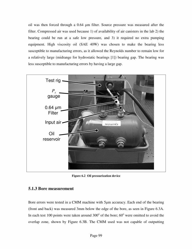
Page 99
oil was then forced through a 0.64 µm filter. Source pressure was measured after the
filter. Compressed air was used because 1) of availability of air canisters in the lab 2) the
bearing could be run at a safe low pressure, and 3) it required no extra pumping
equipment. High viscosity oil (SAE 40W) was chosen to make the bearing less
susceptible to manufacturing errors, as it allowed the Reynolds number to remain low for
a relatively large (midrange for hydrostatic bearings [1]) bearing gap. The bearing was
less susceptible to manufacturing errors by having a large gap.
Ps
gauge
0.64 µm
Filter
Test rig
Input air
Oil
reservoir
Figure 6.2 Oil pressurization device
5.1.3 Bore measurement
Bore errors were tested in a CMM machine with 5µm accuracy. Each end of the bearing
(front and back) was measured 3mm below the edge of the bore, as seen in Figure 6.3A.
In each test 100 points were taken around 300o of the bore; 60o were omitted to avoid the
overlap zone, shown by Figure 6.3B. The CMM used was not capable of outputting

Page 100
arrays of measurement coordinates. Test data was instead reported using error
distribution parameters mean, standard deviation, and min and max measured error.
CMM tip
Template
topology
Clamp
Bearing
front
Bearing rear
5π/3 rad bore
measurement
Overlap
A. CMM measurement setup B. Measurement range around bore
Figure 6.3 Bore precision testing using a CMM
5.2 Stiffness results and discussion 5.2.1 Stiffness test results
The data displayed in Figure 6.4 is the mean displacement of the shaft, derived from
measurements of both capacitance probes. The data from each probe was combined for
ease of graphic representation and because the purpose of the experiment was to measure
the overall bearing stiffness.

Page 101
y = 0.0383x + 0.1613
R2 = 0.99
y = 0.0198x - 0.0159
R2 = 0.9951
y = 0.0388x - 0.0002
R2 = 1
y = 0.0382x - 0.0159
R2 = 0.9951
0
0.5
1
1.5
2
2.5
3
0 10 20 30 40 50 60 70
Force (N)
Dis
pla
ce
me
nt
(mic
ron
s)
Measured data
Theory
Asperity stiffness
Measured, asperitystiffness removed
Figure 6.4 Measured stiffness vs. theory
The initial measured data indicated the bearing was twice as stiff as theory predicted, As
can be seen from Figure 6.4. When the bearing was turned on, the shaft was observed to
deflect down (in the direction of gravity) by approximately 1µm. This indicated that the
shaft was making contact with the bearing bore.
5.2.2 Sources of error in stiffness data
The stiffness of the oil film in Figure 6.4 was obtained by turning off the oil, measuring
the contact stiffness, and removing it from the measured data. The measured data with
asperity stiffness removed is within 1.6% error of the theory.
The contact stiffness and the oil film can be added as springs in parallel if the shaft was
touching the bore at only a few points and not as a Hertzian contact, allowing a full oil
film to develop. This hypothesis was validated by calculating the Hertzian contact
stiffness, which is found to be 48 times greater than the measured contact stiffness.
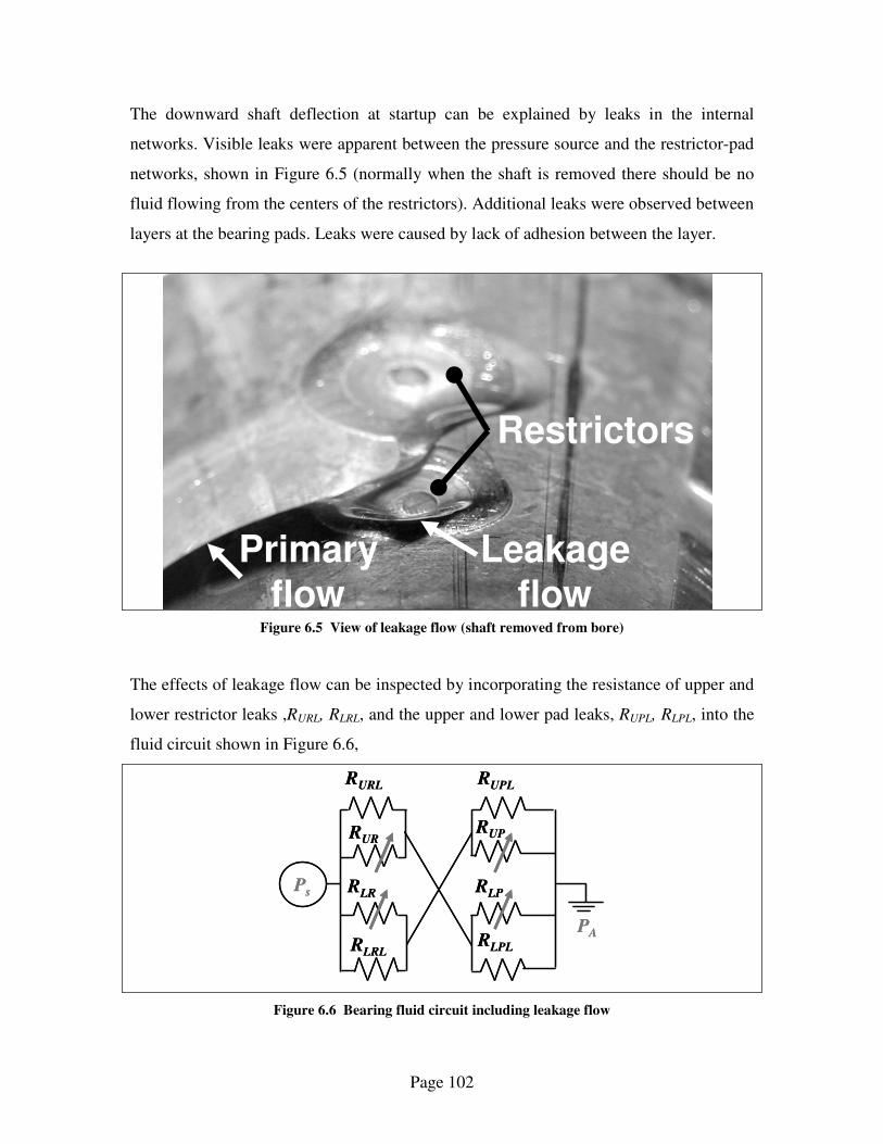
Page 102
The downward shaft deflection at startup can be explained by leaks in the internal
networks. Visible leaks were apparent between the pressure source and the restrictor-pad
networks, shown in Figure 6.5 (normally when the shaft is removed there should be no
fluid flowing from the centers of the restrictors). Additional leaks were observed between
layers at the bearing pads. Leaks were caused by lack of adhesion between the layer.
Leakage flow
Primary flow
Restrictors
Leakage flow
Primary flow
Restrictors
Figure 6.5 View of leakage flow (shaft removed from bore)
The effects of leakage flow can be inspected by incorporating the resistance of upper and
lower restrictor leaks ,RURL, RLRL, and the upper and lower pad leaks, RUPL, RLPL, into the
fluid circuit shown in Figure 6.6,
Ps
RUR
RLPRLR
RUP
RLRL
RURL
PA
RUPL
RLPL
Ps
RUR
RLPRLR
RUP
RLRL
RURL
PA
RUPL
RLPL
Figure 6.6 Bearing fluid circuit including leakage flow

Page 103
Figure 6.7 shows the ideal theoretical stiffness curve with the stiffness curve generated
using the circuit in Figure 6.6.
y = 0.0393x - 0.0289
R2 = 1
y = 0.0393x + 0.0289
R2 = 1
y = 0.0389x + 8.2732
R2 = 0.9995
y = 0.0529x + 11.345
R2 = 0.9967
-15
-10
-5
0
5
10
15
-500 -400 -300 -200 -100 0 100 200 300
Force (N)
Dis
pla
ce
men
t (m
icro
ns
)
Ideal, (+) Disp
Ideal, (-) Disp
Leak, (+) Disp
Leak, (-) Disp
Figure 6.7 Theoretical stiffness with and without leaks
Figure 6.7 shows that a large shift from the neutral position is possible without
significantly changing the bearing stiffness (positive displacement in the direction of
gravity). The leakage gap heights used in generating Figure 6.7 were 101.6µm for the
internal channels at the lower restrictor and 25.4µm for the upper bearing pads. Both of
these values are within the manufacturing tolerance range of the Template. It is important
to note that these leakage values are most likely on the same order as what could be
expected, and are used to demonstrate possible trends that could result from leakage.
Combined effects from the horizontal pads, which could cause further off-center
displacement of the shaft are not included in this analysis.

Page 104
An attempt was made to repair the leakage in the pads. During repair the bearing was
dropped, which warped the bore. Further tests were impossible given that the HBP was
damaged. Also, bearing performance was observed to degrade quickly. The bearing
became non-repeatable and more compliant with successive tests during testing in the
reversed configuration. Increasing compliance would result from increased leakage,
indicating there was adhesive failure between wrapped layers. All data taken after the
first trials was not considered as a result of the mentioned errors.
5.3 Results from bore measurements
Table 6.2 contains the CMM measurement results of the bearing bore. Both ends of the
bearing are within 0.03% of the ideal mean diameter (µD). The front and rear of the
bearing are within 5σ and 2σ, respectively, of the tolerable error range. Although the
precision of the bore is not ideal, it is encouraging that the front of the bearing is 1σ away
from spec, and both ends are within 15.2µm of the desired mean diameter.
Table 6.2 Measurements of bore at front and rear of bearing
Measurement Ideal Bearing front Bearing rear
µ D (mm) 50.902 50.897 50.917
σ(µm) 8.64 7.62 12.70
Max εD(µm) 25.40 12.70 43.18
Min εD(µm) -25.40 -35.56 -20.32
The HBP measured was the first bearing to be adhered with superglue, which made the
wrapping process difficult. The data in Table 6.2 is promising, and with further
refinement and practice of the wrapping and adhesion process the bore will ideally be
made to spec.
5.4 Cost comparison

Page 105
The HBP was compared to a babbitted bearing of similar size and bore surface features
[11] to demonstrate the savings possible with 3DWN technology. Table 6.3 shows a 10X
reduction in cost with 3DWN. Further savings might be possible once a standard 3DWN
manufacturing process is established.
Table 6.3 Cost comparison 3DWN and conventional bearing
Bearing type3DWN Self-Compensated
Hydrostatic
Babbitted Self-
Compensated
Materials $50.00 $30.00
Topology Machining $180.00 $700.00
Housing/Channels Machining $30.00 $5,000.00
Assembly Labor $320.00 $0.00
Total Cost $580.00 $5,730.00
5.5 Summary Although contact between the shaft and bore was observed, the fluid film stiffness
matched theory within 1.6% error after accounting for the contact stiffness. Measuring
the contact stiffness to be much lower than the calculated Hertzian stiffness indicates the
contact occurred only at a few points, which would have still allowed a fluid film to
develop between the bore and shaft.
The mean bore diameter was measured to be within 0.03% error of the mandrel with
errors that lie within 5σ of the tolerable error range in the front of the bearing and 2σ in
the rear. Measurements within 5σ are encouraging. Ideally with more refinement 6σ can
be obtained. As a result of the shimstock used, Table 6.1 shows that the surface finish of
the Template is within the metric defined in Chapter 2.
The most compelling result of this chapter is the cost comparison between 3DWN and
babbitted bearings. Savings could most likely be further increased with improvements
and practice in the wrapping process.
Page 106
CHAPTER
7 SUMMARY
This chapter outlines the scholarly contributions, impact, and future work associated with
this research.
7.1 Scholarly Contributions The following contributions are a result of the work presented in this thesis:
7. A new approach of fabricating low-cost and flexible hysdrostatic bearings –
3DWN technology is a new method of making a precision bearing bore. Surface
replication by wrapping is a deviation from conventional bearing manufacturing
practices; all current fluid film journal bearings require at least one precision
process in their construction.
8. A method of decoupling the fabrication processes from the precision requirements
of the bearing – In the 3DWN manufacturing process the errors associated with
the non-precision parts have less of an effect on bearing performance then errors
in the precision parts. This is powerful, in that it supports the feasibility of 3DWN
technology by showing a hydrostatic bearing’s precision requirements can be
decoupled from the fabrication processes used to make it.
9. Metrics to judge the required precision of off-the-shelf parts used in 3DWN
technology – Metrics to judge the level of precision required in the off-the-shelf
parts used to make a 3DWN bearing are defined from conventional hydrostatic
bearing theory.

Page 107
10. A new process of manufacturing parts with internal features – 3DWN is a new
process of making parts with internal features. 3DWN is not limited to fluid
channels; it could be used for many kinds of applications that require cylindrical
internal networks.
11. A model to describe a wrapped structure – A model for describing a wrapped
structure is derived. This model enables coordinates in a 3D cylindrical structure
to be transformed to a 2D Template. When the Template is rolled, the 2D features
align in the wrapped structure to recreate the original 3D features.
12. A means of converting 3D bearing geometry to 2D features – Existing bearing
features are modified such that it can be cut into a 2D Template. Conventional
hydrostatic bearing analysis is used to evaluate the bearing performance.
7.2 Engineering impact The results of this thesis may impact engineering applications in the following ways:
1. An order of magnitude cost reduction from current bearings – The cost
comparison in this thesis demonstrates a 10X reduction in cost from a babbitted
bearing to a 3DWN bearing of the same sized and topology. Reducing the cost of
hydrostatic bearings by an order of magnitude would facilitate their use in more
engineering applications.
2. A flexible process in which to design and fabricate hydrostatic bearings – 3DWN
technology could provide great flexibility in manufacturing and design of custom
hydrostatic bearings. When the 3DWN manufacturing process is perfected, a
flexible bearing fabrication machine could be designed which makes any size
bearing by simply switching the mandrel size. As a result hydrostatic bearings
would not be “one-off” designs, which would further lower the cost of production.
Page 108
3. A hybridization between 3DWN and current bearing technology – 3DWN
technology is an ideal method of producing self-compensated bearings because
the internal channels are cut at the same time as the bearing topology. As was
seen in the cost comparison in Chapter 6, the major cost in producing the
babbitted bearing was the manufacturing internal channels. 3DWN-conventional
hybrid bearings could possibly be produced by wrapping a template around a
cylinder that already has the required bore precision, for example a bronze
bushing.
4. A low-cost method of producing precision bores – Precision bore wrapping could
have other applications beyond hydrostatic bearings. One possible application
could be in hydrodynamic bearings. The overlap region of a 3DWN structure
could stagnate the gas flow in the bearing, causing a high pressure zone. The
overlap region could also be used as a feed for lubrication, similar to the notches
in hydrodynamic bearings found in IC engines.
5. Expansion of 3DWN technology to other products – 3DWN technology could be
expanded to other applications that require internal networks. Some of these
applications, currently being explored by the author, are fuel cells and circuit
boards. The cylindrical shape of 3DWN structures makes them a possibility for
use in applications such as batteries, missiles, or medical implants in the
circulatory system.
7.3 Future work The following areas of research would increase the feasibility of hydrostatic bearings
being made using 3DWN technology.
1. Possible adhesives for bonding wrapped layers needs to be further researched. As
was described in Chapter 4, many methods of adhering the HBP were attempted

Page 109
without success. Adhesive films still may be a possible solution with
parameterization of their flow characteristics.
2. Most of the design effort in the HBP was focused on the topology and not the
internal features. Internal feature layout could be optimized to insure better
adhesion between layers, which would reduce the likelihood of leaks.
3. Alternative cutting processes should be explored beyond waterjet cutting. Laser
cutting is attractive because 1) it is low cost 2) it is faster than waterjet cutting, 3)
it doesn’t require protective layers of plastic sandwiching the template, and 4) it
leaves a bur on only one side. Inert environment laser cutting may be an option
for manufacturing bronze Templates.
4. To save manual labor time, chemical deburring and etching processes should be
explored. To enable chemical deburring, the Template could be cut with a plastic
film covering the bearing surface. When dipped into the chemical bath, the plastic
film would protect the bearing topology from becoming etched.
5. Better methods of fixturing the Template to the mandrel should be explored. The
hose clamps scratched the surface of the mandrel during fabrication of the HBP,
which is undesirable for mandrel re-use in multiple bearings. Also, the sacrificial
tabs have to be carefully removed, as to not damage the bore. Possible methods of
fixturing could include vacuuming the Template in place, or loosely wrapping
multiple layers and using a capstan effect to tighten them against the mandrel.

Page 110
REFERENCES [1] Slocum, Alexander H. Precision Machine Design. Dearborn: Society of
Manufacturing Engineers, 1992. [2] Bassani, R., Piccigallo, B., Hydrostatic Lubrication. Amsterdam: Elsevier, 1992. [3] Geary, P. G. Fluid Film Bearings. Kent: British Scientific Instrument Research
Association, 1962. [4] Kotilainen, M.S.A. Design and Manufacturing of Modular Self-Compensating
Hydrostatic Journal Bearings. MIT Ph.D. Thesis in Mechanical Engineering, Massachusetts Institute of Technology, Cambridge, 2000.
[5] Kotilainen, M.S, Slocum, A.H. "Manufacturing of cast monolithic hydrostatic journal
bearings." Precision Engineering. 25 (2001): 235-244. [6] Wasson, K.L. Hydrostatic Machine Tool Spindles. MIT PhD. Thesis in Mechanical
Engineering, Massachusetts Institute of Technology, Cambridge, 1996. [7] Wasson, K.L. “TurboTool.” Precision Engineering Research Group. MIT. 10 Mar.
2005 <http://pergatory.mit.edu/>. [8] Slocum, A., Wasson, K. "Tooling System and Method with Integral Hydrostatic
Bearings and Turbine Power Source". Patent #5,674,032. 7 Oct. 1997. [9] Wasson, K.L, Slocum, A.H, "Integrated Shaft Self-Compensating Hydrostatic
Bearing". Patent #5,700,092. 23 Dec. 1997. [10] Avallone, E.A., Baumeister III, T. Marks’s Standard Handbook for Mechanical
Engineers. New York: McGraw-Hill, 1996. [11] Conversations with Bill Chappell, Babbitt Bearings, Inc. 6 Jun. 2005. 734 Burnet
Ave., Syracuse, NY 13203. [12] Lyon, G.S. “Self-compensating hydrostatic bearing with tape”. US Patent
#6,012,845. 11 Jan. 2000. [13] Girard, L. D. Noveau Système de Locomotion sur Chemin de Fer. Machelier, Paris.
1852. [14] Sonin, A. Notes on Fully Developed Flow. MIT Class 2.25: Advanced Fluid
Mechanics. 15 Jan. 2005. <http://stellar.mit.edu/S/course/2/fa04/2.25/index.html>. [15] Slocum, A. "Self Compensating Hydrostatic Linear Bearing". US Patent
#5,104,237. 14 Apr. 1992.

Page 111
[16] Stansfield, F. Hydrostatic Bearings for Machine Tool and Similar Applications.
London: The Machinery Publishing Co., 1970. [17] Gross, W.A. Gas Film Lubrication. New York: John Wiley and Sons, Inc., 1962. [18] Stout, K.J., Barrans, S.M., “The design of aerostatic bearings for application to
nanometer resolution manufacturing machine systems.” Tribology International. 33 (2000): 803-809.
[19] Fox, R.W, McDonald, A.T. Introduction to Fluid Mechanics. New York: John
Wiley and Sons, Inc., 2003. [20] Khonsari, M.M., Booser, E.R. Applied Tribology: Bearing Design and Lubrication.
New York: John Wiley and Sons, Inc., 2001. [21] Whitehouse, D. Surfaces and their Measurement. New York: Taylor and Francis,
2002. [22] Slocum, A. "Self-Compensating Hydrostatic Bearings for Supporting Shafts and
Spindles and the Like for Rotary and Translational Motion and Methods Therefore". US Patent #5,281,032. 25 Jan. 1994.
[23] Slocum, A.H., et al. “Design of Self-Compensated Water Hydrostatic Bearings”.
Precision Engineering. 17 (1995): 173-185. [24] Young, W.C., Budynas, R.G. Roark’s Formulas for Stress and Strain. New York:
McGraw-Hill, 2002. [25] Kundu, P.K., Cohen, I.M. Fluid Mechanics. Amsterdam: Elsevier Academic Press,
2004. [26] “9244 Structural Building Tapes.” 3M. 15 Aug. 2004 <
http://products3.3m.com/catalog/us/en001/manufacturing_industry/converter_markets/node_MR3CCGK4BJbe/root_GST1T4S9TCgv/vroot_NZJMNZVQR6ge/gvel_H0GZC75S2Wgl/command_AbcPageHandler/theme_us_convertermarketsinternet_3_0/>.
[27] “AF 163-2 Sotch-Weld: Structural Adhesive Film.” 3M. 20 Mar. 2005. <
http://products3.3m.com/catalog/us/en001/government/innovative_solutions/node_GSNFN8VMQHbe/root_GS3RBW6QFVgv/vroot_31S2JJ7584ge/gvel_HK9RDD0JZTgl/command_AbcPageHandler/theme_us_innovativesolutions_3_0/>.
[28] ”3M Scotcast Electrical Resin.” 3M. 10 Feb. 2004. <
http://products3.3m.com/catalog/us/en001/utilities_telecom/oem_electrical/node_G
Page 112
SGMZ9BC8Gbe/root_GST1T4S9TCgv/vroot_GSHBRQT7DVge/gvel_FBPVWXK14Zgl/command_AbcPageHandler/theme_us_oemeletrical_3_0/>.