, U A P T f i " : f%• H IHI ■ I w iWg^P

Design of Knowledge Base and Sensitivity

Evaluation of I D M T Relay

5.1 In troduction

5.2 Fuzzification o f ID M T C urve

5.3 Rule Base Design

5.4 Rule Base Inference

5.5 Sensitivity E valuation of Fuzzy Sensor

5.6 Rule Base F iring Process

5.7 Sim ulation R esults

5.8 Discussion

" To see a world in a grain of sand, and heaven in a wild flower. Hold infinity in the palm of

your hand, and eternity in an hour."

William Blake

Chapter 5 .

Design of Knowledge Base and Sensitivity Evaluation of IDMT Relay

5.1. IntroductionIn chapter 4 , rule base design (Of IDMT relay) for the variables available at the input part of

the fuzzy system has been discussed for only three FAM rules .The output o f this system was very rough

and undesirable. This can be avoided by increasing the number o f rules. Each fuzzy predicate for the

sensor designed in chapter 4 has been subdivided into three more linguistic predicates and the rule base

has been modified to obtain nine rules. The performance o f fuzzy sensor has been tested by evaluating

its sensitivity. A model for sensitivity evaluation o f fuzzy sensor has been proposed to work in 26 rules.

A computer simulation has been conducted and the simulation results have been discussed. The

procedure has been explained under the subsequent headings and subheading o f this chapter.

5.2. Fuzzification of IDMT CurveThe characteristics curve o f IDMT relay shown in Fig. 4.5 in last chapter have again fuzzified by

subdividing into nine more linguistic predicates and the modified curve is shown in Fig. 5.1 .

Each of linguistic predicates low, medium and high are subdivided into three more predicates as

listed below [72,109,114]:

(i) Predicate small is subdivided into very small, small and slightly sm all.

(ii) Predicate medium is subdivided into slightly medium, medium and high medium.

(iii) Predicate high is subdivided into slightly high, high and very high

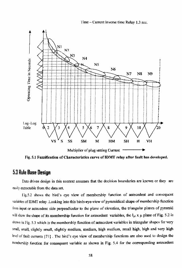
Time - Current Inverse time Relay 1.3 sec.

Multiplier o f plug setting Current ----------------►

Fig. 5.1 Fuzzification of Characteristics curve of IDMT relay after fault has developed.

5.3 Rule Base DesignData driven design in this context assumes that the decision boundaries are known or they are

easily extractable from the data set.

Fig.5.2 shows the bird’s eye view o f membership function o f antecedent and consequent

variables of IDMT relay .Looking into this birds-eye-view o f pyramidical shape o f membership function

from input or antecedent side perpendicular to the plane o f elevation, the triangular planes o f pyramid

will show the shape o f its membership function for antecedent variables, the Ipi x p. plane o f Fig. 5.2 is

shown in Fig. 5.3 which is the membership function o f antecedent variables in triangular shapes for very

small, small, slightly small, slightly medium, medium, high medium, small high, high and very high

level of fault currents [71] . The bird’s eye view of membership functions are also used to design the

membership function for consequent variable as shown in Fig. 5.4 for the corresponding antecedent

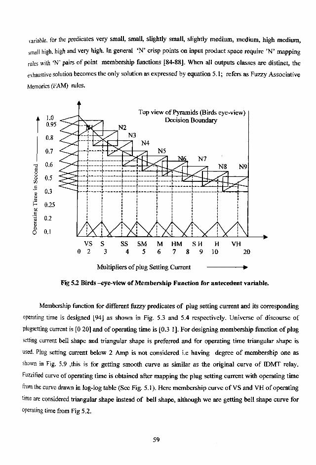
variable, fo r the predicates very small, small, slightly small, slightly medium, medium, high medium,

sm all h igh , h ig h and very high. In general ‘N’ crisp points on input product space require ’N ’ mapping

rules w ith ‘N’ pairs of point membership functions [84-88]. When all outputs classes are distinct, the

exhaustive s o lu t io n becomes the only solution as expressed by equation 5.1; refers as Fuzzy Associative

M em ories (FAM) rules.

0 2 3 4 5 6 7 8 9 10 20

Multipliers o f plug Setting Current ---------------- ►

Fig 5.2 Birds -eye-view of M embership Function for antecedent variable.

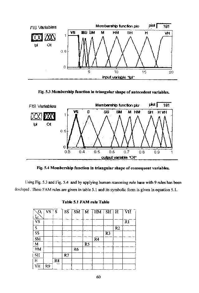
Membership function for different fuzzy predicates o f plug setting current and its corresponding

operating time is designed [94] as shown in Fig. 5.3 and 5.4 respectively. Universe o f discourse of

plugsetting current is [0 20] and o f operating time is [0.3 1]. For designing membership function o f plug

setting current bell shape and triangular shape is preferred and for operating time triangular shape is

used. Plug setting current below 2 Amp is not considered i.e having degree o f membership one as

shown in Fig. 5.9 ,this is for getting smooth curve as similar as the original curve o f IDMT relay,

Fuzzified curve of operating time is obtained after mapping the plug setting current with operating time

from the curve drawn in log-log table (See Fig. 5.1). Here membership curve o f VS and VH o f operating

time are considered triangular shape instead o f bell shape, although we are getting bell shape curve for

operating time from Fig 5.2.

FIS Variables

o t

Membership function plo pl°t | 181

input variable ipl"

Fig. 5.3 Membership function in triangular shape of antecedent variables.

FIS Variables Membership function plo- Pj°* | 181

Ipl Ot

output variable ’O f

Fig. 5.4 Membership function in triangular shape of consequent variables.

Using Fig. 5.3 and Fig. 5.4 and by applying human reasoning rule base with 9 rules has been

developed. These FAM rules are given in table 5.1 and its symbolic form is given in equation 5.1.

Table 5.1 FAM rule Table

\ p tV \

VS S SS SM M HM SH H VH

v s R1s R2ss R3SM R4M R5HM R6SH R7H R8VH R9

Ipl • P v s-----------------------------► Ot «PvH ^

Ipi • Ps -----------------------------► Ot *P h

Ipl • Ps S ► Ot »P sh

Ipl • Ps M ^ Ot «P hm

Ipi*Pm ^ O t *P m V . . . ( 5 .1 )

Ipl*PHM ^ O t *PsM

Ipl *PS H ^ O t* P sS

Ipl* P h -----------------------------► O t . P s

Ipl *PvH ^ O t • P vs

Inequation 5.1 Ipi represents Plug setting current level.

Ot represents Operating time of relay

P v s represents Predicate very Small

P s represents Predicate Small

P ss represents Predicate slightly Small

PsM represents Predicate slightly Medium

P m represents Predicate medium

P hm represents Predicate highly medium

PSH represents Predicate slightly high

P h represents Predicate high

P vh represents Predicate very high

• represents Symbol for ‘IS’

-► represents Symbol for ‘THEN’

Equation 5.1 is used to design the FAM rules o f inference system o f fuzzy sensor . These FAM rules

can be written in linguistic form[13] as given below, Fig. 5.5 depicts the rule base development using

MATLAB software [41].

FAM R ulel: IF plug setting current level is very small THEN operating time for relay is very High.

FAM Ruke2 :IF plug setting current level is small THEN operating time for relay is High.

FAM Rule3: IF plug setting current level is slightly small THEN operating time for relay is slightlyHigh.

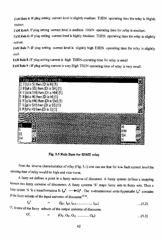
FAM Rule 4: IF plug setting current level is slightly medium THEN operating time for relay is Highly

Medium.

FAM Rule5: IF plug setting current level is medium THEN operating time for relay is medium.

FAM Rule 6: IF plug setting current level is highly Medium THEN operating time for relay is slightly

medium.

FAM Rule 7: IF plug setting current level is slightly high THEN operating time for relay is slightly

small.

FAM Rule 8 :IF plug setting current is high THEN operating time for relay is small

FAM Rule 9 : IF plug setting current is very High THEN operating time o f relay is very small.

1. If flpl is V S | then fO U s V H I [12. If(lpl is S] then (Q t is H ) (1 )3. If (Ipl is SS) then (Ot is S H ) (1)4. If (Ipl is SM) then (Ot is H M ) (1)5. If (Ipl is M ) then (Ot is M ] (1)6. If (Ipl is H M ) then (Ot is S M ) (1)7. If (Ipl is SH) then (Ot is S S ) (1)8. If (Ipl is H) then (Ot is S) (1)

Fig. 5.5 Rule Base for IDMT relay

From the inverse characteristics o f relay (Fig. 5.1) one can see that for low fault current level the

operating time of relay would be high and vice-versa.

A fuzzy set defines a point in a fuzzy universe o f discourse. A fuzzy system defines a mapping

between two fuzzy universe o f discourses. A fuzzy systems ‘S’ maps fuzzy sets to fuzzy sets. Thus a

fuzzy system S is a transformation S: Ipin ►Otp . The n-dimensional units hypercube Ip" contains

all the fuzzy subsets of the input universe of discourse10,16.

*P' = (Ipll, IpI2,IpL3,...................... Ipin) . . . (5 .2 )

0 1 houses all the fuzzy subsets o f the output universe o f discourse.

° Pt = (O ti O c 0 ( 3 , .................Otn) . . .(5 .3 )

They map close inputs to close outputs, which are referred as fuzzy associative memories or FAMs, The

FAM rule8.

IF ‘Isp, ‘is ‘Ps- THEN Os, IS PH ...(5.4)

May be encoded by (Ps, Ph)

In general a FAM system F: InPi---- ► Opt encodes and processes in parallel a FAM bank o f FAM rules.

(Psi, Phi) , (Ps2, PmX (Ps3, Pro)................. (Psm, Phm) . ...(5.5)

Fuzzy systems estimate functions with fuzzy set samples (Psi,PHi), neural samples use numerical-

point samples. Engineers sometimes call the fuzzy set association (PSl> Pm) a “rule” . Here PSi is referred

as antecedent term and PHi is referred as consequent term. The antecedent variables with referred to

membership function would be -

The corresponding consequent variables would be -,n VH n SH n HM n HM n M n M n SM n SM ^ S S n SS ^ V S ^ V S x ~(O t i U q KJ t3sU t4, ^ t l , vJ t2, ^ t3 ,U t4 ,U tl t3 , ^ t4 J . . . (5 .7 )

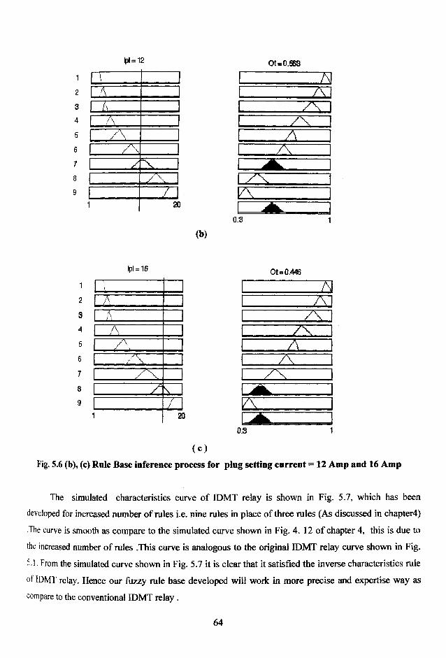
5.4 Rule Base InferenceFig. 5.6 (a),(b) and (c) illustrates the rule firing process and its corresponding outcome for

different plug setting currents i.e for 4 Amp, 12 Amp and 16 Amp respectively. As it is clear from above

figure that if plug setting current is increasing operating time is decreasing and vice-versa.

|P,=4 Ot=0.882

1

2 / ......... ~ K3 “ ;....“ " " A .4 A .......... " A .5

— ^---------------------

6 " A - " '7 _____ ______8 : : ' ; : 2 i z / \ ......... ...

9 ....................... ~ r~ a ...............1 20

..........0.3 1

Fig. 5.6 (a) Rule Base inference process for plug setting current = 4 Amp.

'1 .. ,AA „ . „

a;- ......./ \T V

■“TV/ \N /Ky \

/20

a

z s ::zz:z n

z z

z x

0.3(b)

lp, = 16 Ot=0.446

L..... . ..... L ' : ; : : : . ' ' ' aA/ \ ........ A, .L _________ .................... w"■ /•; .........t \ ' .... .. .......

........ . _ z _ . : z \ _ . . :/ \

..........................z 1>>. M . " ..................z : A '

1 200.3 1

(c)Fig. 5.6 (b), (c) Rule Base inference process for plug setting current = 12 Amp and 16 Amp

The simulated characteristics curve o f IDMT relay is shown in Fig. 5.7, which has been

developed for increased number o f rules i.e. nine rules in place o f three rules (As discussed in chapter4)

•The curve is smooth as compare to the simulated curve shown in Fig. 4. 12 o f chapter 4, this is due to

the increased number o f rules .This curve is analogous to the original IDMT relay curve shown in Fig.

5.1. From the simulated curve shown in Fig. 5.7 it is clear that it satisfied the inverse characteristics rule

of IDMT relay. Hence our fuzzy rule base developed will work in more precise and expertise way as

compare to the conventional IDMT relay .

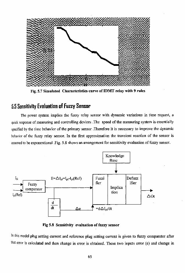
Fig. 5.7 Simulated Characteristics curve of IDMT relay with 9 rules

5.5 Sensitivity Evaluation of Fuzzy SensorThe power system implies the fuzzy relay sensor with dynamic variations in time request, a

quick response of measuring and controlling devices .The speed o f the measuring system is essentially

specified by the time behavior o f the primary sensor .Therefore it is necessary to improve the dynamic

behavior of the fuzzy relay sensor. In the first approximation the transient reaction o f the sensor is

assumed to be exponentional .Fig. 5.8 shows an arrangement for sensitivity evaluation o f fuzzy sensor.

Fig 5.8 Sensitivity evaluation of fuzzy sensor

In this model plug setting current and reference plug setting current is given to fuzzy comparator after

that error is calculated and then change in error is obtained. These two inputs error (e) and change in

error (Ae) are supplied to inference engine , which produces corresponding change in operating time

(AOt) after fuzzification , implication through rule base and defuzzification.

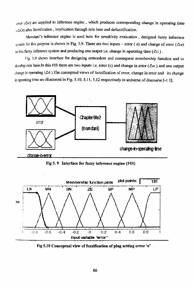
Mamdani’s inference engine is used here for sensitivity evaluation , designed fuzzy inference

svstem for this purpose is shown in Fig. 5.9. There are two inputs - error ( e) and change o f error (A e)

in this fuzzy inference system and producing one output i.e. change in operating time ( A t ) .

Fig. 5.9 shows interface for designing antecedent and consequent membership function and to

develop rule baseJn this FIS there are two inputs i.e. error (e) and change in error (A e ) and one output

change in operating (A t ).The conceptual views o f fuzzification o f error, change in error and its change

in operating time are illustrated in Fig. 5.10, 5.11, 5.12 respectively in universe o f discourse [-1 1].

Membership lunction plots p*°* P°'nts- | 181

input variable Terror"

Fig 5.10 Conceptual view of fuzzification of plug setting error ‘e’

Mem bership function plots p ot P°'nts: j 181

input variable ■tehange-in-error"

Fig 5.11 Conceptual view of fuzzification of change in error ‘ A e’

Membership function plots p*ot P °ints: f 181

output variable ‘thange-in-operating-time

Fig 5.12 Conceptual view of Fuzzification of change in operating time ‘A t’

Table 5.2 Rule base development (FAM Rule)

Using Table 5.2 one can develop 31 rules for sensitivity testing o f fuzzy sensor as given

below in linguistic form

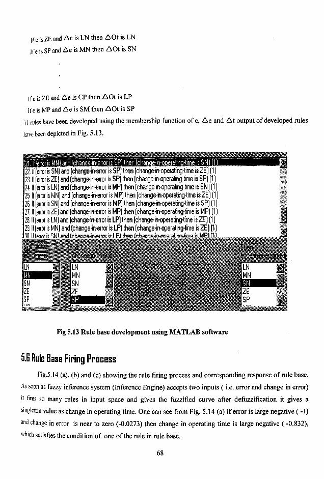
If e is ZE and Ae is LN then A O t is LN

If e is SP and Ae is MN then A O t is SN

If e is ZE and Ae is CP then A O t is LP

If e is MP and Ae is SM then A O t is SP

31 rules have been developed using the membership function o f e, A e and A t output o f developed rules

have been depicted in Fig. 5.13.

1, il [error is MN] and [chanqe-in-error is SF'j then Ichange-in-operating-time is,SN i,.Ll,22. If (error is SN] and (change-in-error is SP] then (change-in-operating-time is ZE) (1]23. If (error is ZE) and (change-in-error is SP) then (change-in-operating-time is SP] (1)24. If (error is LN j and (change-in-error is MP) then (change-in-operating-time is SN) (1)25. If (error is MN) and (change-in-error is MP) then (change-in-operating-time is ZE) (1)26. If [error is SN) and (change-in-error is MP) then (change-in-operating-time is SP) (1)27. If (error isZE) and (change-in-error is MP) then (change-in-operating-time is MP) (1)28. If (error is LN j and (change-in-error is LP) then (change-in-operating-time is ZE) (1)29. If (error is MN] and (change-in-error is LP) then (change-in-operating-time is ZE) (1)I d If fp rrn r k ^ N l a n d ^ 1

and

m m m rSNZESP

chanqe-in-errof is

LN a

MN “SN ^ZE

Then-in-ope

[LNMNSNZESP

Fig 5.13 Rule base development using MATLAB software

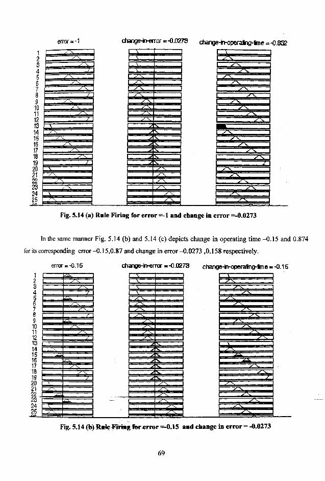
5.6 Rule Base Firing ProcessFig.5.14 (a), (b) and (c) showing the rule firing process and corresponding response o f rule base.

As soon as fuzzy inference system (Inference Engine) accepts two inputs ( i.e. error and change in error)

it fires so many rules in input space and gives the fiizzified curve after defuzzification it gives a

singleton value as change in operating time. One can see from Fig. 5.14 (a) if error is large negative ( -1)

and change in error is near to zero (-0.0273) then change in operating time is large negative (-0.832),

which satisfies the condition o f one o f the rule in rule base.

12345678910 11 121314151617181920 21 22232425nr.

i i a : ... -------------------- 1X X — I 1 .. 1.1,11,— ,11, ____________1t j - s:---------- .. - " " " I

----------- -- ----------- ! 1 I 7 -----------i i y - v - J

, s. L y ^ . --------------------1/ \ 1 1 ^ ____________1

-------- 7"\ 1....1 r - ‘ mjrr?

x ^ _ _ « i x vi f— 7 ^ '

--------------z_< i--------- ^a i r- - . . - 3 ^ ...: 1

1 I V- i | /

/ \ i p p ■V.^ --------- , i— x

./■<. 11 1” .........~ J V .................- 1 i > -X

V ---------------------1 i—i r * “ ...i i ................... ______

....... i r ~ ' ” V ' V ......._ A ------------------------------- 1 I------------------ ........X X

- " ' ' 1 1 ’ "......... . ' —

change-in-operalng-fme=-0.832 r —

7 V

~ ? ^ r

iZ X

z s ;I

"7TT

z x ;

r ^ rz s

.... . »

Fig. 5.14 (a) Rule Firing for error =-1 and change in error =-0.0273

In the same manner Fig. 5.14 (b) and 5.14 (c) depicts change in operating time -0.15 and 0.874

for its corresponding error -0.15,0.87 and change in error -0.0273 ,0.158 respectively.

12345678910 11 121314151617181920 21 22 23

error = -0.15

24 C

change-in-error = -0.0273.. ..... . '“ "'I

------- 1 1 ... _________ 1■ ^ ” 1 r t ■■...-""I

-' i l AJ L X. v -----

-------1 -----_____ I. ....................................... .

'■ ' 7 1 I" ...^ . — 1 I-------^

..--X 1 . X X1 1

________ L J 1_____^1 v. .............I 1.......... v ..... ....1

----------------1 1----------- X ■v 1

^ 1 L ------^ ---------- 1. J L_______* \ "'1 1......... v ^ — ------- 1

> 1 1 Xr 1 J > X i1 .-"s • I

--------------- 1 1------------- v x 1 I' 1 — i . . s \ ..... . ""1

r •, i i - .^X 1i i i ........ .... -1

change-in-operaing~fme =-0.15 i " v~----------------- 1

ar z x :

zs:zs:

Big. 5.14 (b) f t ik Firing for error =-0.15 and change in error = -0.0273

12345678910 11

14151617181920 21 22232425(VI

1 ------------------------ 1 L _ E -------------------" 1— i — 1

1 ------------------------------- i - i — J L J i ________________ 1

1— 1 1 c . . . y . . . k i

1— . ^ J L X . ' . ' - , . '7 ^ ' ■ i

1— . . - - X . - J -------------------- ------------------ 1

r J -------------------- i ^ |

f . . ^ J ___________ 1__________________ ^ „ , 1

r : 2 “ | | f \ " 1 r r ...... ................ ^ i1 ----------------------- • L 1 11 ------------------------------- ^ — 1 1 ^ . . . .

I - i L - i ^ i

___________________________________ i J 1___________ i -----------------------------------------------------

i \ ; j r .....■ ......- 2 ^ i \ ■ ................................. ■ i

i . J L . I ..... i 1i _ J C T T .... . ~ 2 5 i ^ i

i . J r _ - - T 2 5 1 1

1 . - v - . . , , . J 1----------------------------- i - - i

i ' - i t ; - ................. - ' r ~ ........................ ....\

r ™ . ....z s * 1 ------------------------------------Z J

i ....................- ■ » i " , ........... ................. ■ i i

i - i i - .............. s — i ^ -----------------------------------------1

1 ■ _____________ i ■ ■ ^ >

1 . / v ' I r - - ..... ^ ------------------ | ............ “ T V --------------- 1

1......\ i | j s \ _ 1 ^ 1

__________________________ i i _ - - V 1 i ------------------- _ . _ l

( C )

Fig. 5.14 (a) Rule Firing for error =0.87 and change in error =0.158

Fig.5.15 depicts the three dimensional pictorial view for error e ,change in error A e and change in

operating time AtFrom this figure one can obtain the output for different inputs .

change-in-error

Fig 5.15 Three dimensional surface viewer of input and output of FIS

The step response can be described by a single or by a combination o f several error-functions. In

the proposed new method for improving the dynamic response o f the slow plug setting current sensor

shall b e presented.The operating time ‘Ot’ of the sensor is controlled as output variable o f a fuzzy sensor with the

two input variables, plug setting current difference (A Ipi )and its dynamic change with respect to time

(dA Ip i/d t ). The control scheme is shown in Fig. 5.8. The decision making or fuzzy reasoning is

p erfo rm ed using table 5.2 constructing rules for rule base .

The fuzzy sensor working in following three steps :

(i) Fuzzification

(ii) Fuzzy inference

(iii) De-fuzzification

The functions are performed by application o f fuzzy -variables, membership function and

control rules .The small positive (SP), medium positive(MP), large positive(LP), zero(ZE), negative

small (NS), medium negative (MN), and large negative (LN) are fuzzy linguistic values for fuzzy

variables i.e. change in plug setting current, dynamic change o f plug setting current and change in

operating time .These linguistic values must be determined by experimental and subjective knowledge.

The fuzzification means the linguistic interpretation o f technical quantity in general, plug setting

currents and operating time in particular. The defuzzification correspondingly in the transformation of a

linguistic term into a technical quantity, particularly the feeding current o f the sensor, the influences

draws the conclusions from the knowledge base, which fulfill the qualification according to the

membership functions.

5.7 Simulation ResultsAt first the procedure presented has been simulated with P-IV machine, where the plug setting

currents losses in the sensor are not taken into account .The result is shown in Fig. 5.16.

Fig.5.16 shows that the final plug setting current o f the fuzzy sensor is reached in comparison to

the conventional sensor within considerable short time .For an experimental test a relatively great and

slow sensor of type CDG 11 manufactured by GEC Alsthom, India, has been applied and has been fed

with a fuzzy plug setting current. The experimental result o f the fuzzy sensor which is operated with

fuzzy plug setting current is shown in Fig.5.17. It is evident that the final plug setting is already reached

after the first few amperes o f plug setting current .After switching o ff the plug setting current the current

decreases on account o f losses compensation effects within the fuzzy sensor .

After a m in im u m value the sensor is allowed to pass current again and the current rises .The process

is repeated u n til the final plug setting current is reached.

Fuzzy sensor response

Time in sec.----------►

Fig. 5.16 Simulation of fuzzy controlled relay sensor

Time in sec. ------------------------ ►

Fig. 5.17 Experimental result of fuzzy relay sensor response

5.8 Discussion

In this chapter characteristics curve o f IDMT relay is fuzzified using nine fuzzy predicates

instead of three (As discussed in chapter 4) to check the performance o f IDMT relay as fuzzy sensor.

Result has been found satisfactory, the curve simulated thus is smooth (See Fig. 5.7) as compare to the

curve sim u lated using three rules (See Fig. 4.12).

A fuzzy sensing conception has been realized for improving the dynamic response o f a slow plug

setting current sensor. Simulation and experiments show that the sensor response can forced by a fuzzy

plug setting current which accelerates the step response time evidently although the procedure described

is only qualified for positive rise o f temperature, the resulting dynamic performance is evidently

improved.