design of lean bernoulli lines · design of lean bernoulli lines motivation: designers of...

Chapter 6

Design of Lean BernoulliLines

Motivation: Designers of manufacturing systems select machines for produc-tion lines based on their technological characteristics. Material handling devicesare selected based on the nature of parts produced, available space, type of pro-duction, etc. Their capacity, in their function as in-process buffers, is typicallyselected as small as possible, i.e., lean. But how lean can lean buffers be? Inother words, what is the smallest buffer capacity, which is necessary and suffi-cient to ensure the desired production rate of a system? This is the questionaddressed in this chapter.

Overview: Closed formulas for lean buffering in systems with identical Ber-noulli machines are derived. These formulas are exact for two- and three-machine lines and approximate for longer lines. For the case of non-identicalBernoulli machines, both closed-form expressions and recursive approaches aredeveloped.

6.1 Parametrization and Problem Formulation

Consider a serial production line with Bernoulli machines defined by conventions(a)-(e) of Subsection 4.2.1. Introduce the following notions:

Line efficiency (E) – production rate of the line, PR, in units of the largestpossible production rate of the system.

As it is clear from Chapter 4, the largest production rate is obtained whenall buffers are infinite. Denote this production rate as PR∞. Then, the lineefficiency can be expressed as

E =PR

PR∞=

PR

min{p1, . . . , pM} . (6.1)

Obviously, 0 < E < 1.

201

202 CHAPTER 6. DESIGN OF LEAN BERNOULLI LINES

Lean buffer capacity (LBC) – the sequence

N1,E , . . . , NM−1,E (6.2)

such that the desired line efficiency E is achieved while∑M−1

i=1 Ni,E is minimized.In other words, LBC is the buffer capacity, which is necessary and sufficient toobtain the desired PR, quantified by E.

The problem addressed in this chapter is to develop analytical methods forcalculating LBC as a function of machine efficiencies pi, i = 1, . . . , M , lineefficiency E, and the number of machines in the system M . For the case ofidentical machines, i.e., pi =: p, i = 1, . . . ,M , this is carried out in Section 6.2,while the case of non-identical machines, pi 6= pj , i, j = 1, . . . , M , is addressedin Section 6.3.

6.2 Lean Buffering in Bernoulli Lines withIdentical Machines

In this section, we assume that all machines have identical efficiency,

pi =: p, i = 1, . . . , M, (6.3)

and, in addition, all buffers are of identical capacity,

Ni =: N, i = 1, . . . ,M − 1. (6.4)

Assumption (6.4) is introduced in order to obtain a compact representationof the results. It should be pointed out that a more efficient buffer capacityallocation in systems satisfying (6.3) is the inverted bowl pattern (see Chapter5). However, this leads to just a small improvement of the production rate incomparison to the uniform allocation (6.4) (typically, within 1%) and, therefore,is not considered here.

6.2.1 Two-machine lines

In the case of two identical machines, expression (4.19) for the production ratebecomes

PR = p[1−Q(p,N)], (6.5)

where, as it follows from (4.14),

Q(p, N) =1− p

N + 1− p. (6.6)

Thus, using (6.1), we obtain

PR = PR∞E = p[1−Q(p, NE)], (6.7)

6.2. LEAN BUFFERING FOR IDENTICAL MACHINES 203

where NE is the buffer capacity necessary and sufficient to ensure E. Takinginto account that PR∞ = p, (6.6) and (6.7) result in the following equation:

E = 1− 1− p

NE + 1− p. (6.8)

Solving for NE and taking into account that NE is an integer, we obtain

Theorem 6.1 The lean buffer capacity in Bernoulli lines defined by as-sumptions (a)-(e) of Subsection 4.2.1 with M = 2 and p1 = p2 =: p is givenby

NE(M = 2) =

⌈E(1− p)1− E

⌉, (6.9)

where dxe denotes the smallest integer not less than or equal to x.

Note that according to (6.9), NE cannot be less than 1. Under the blockedbefore service assumption, buffering NE = 1 implies that the machine itselfstores a part being processed and no additional buffering between the machinesis required. This can be interpreted as Just-in-Time (JIT) operation.

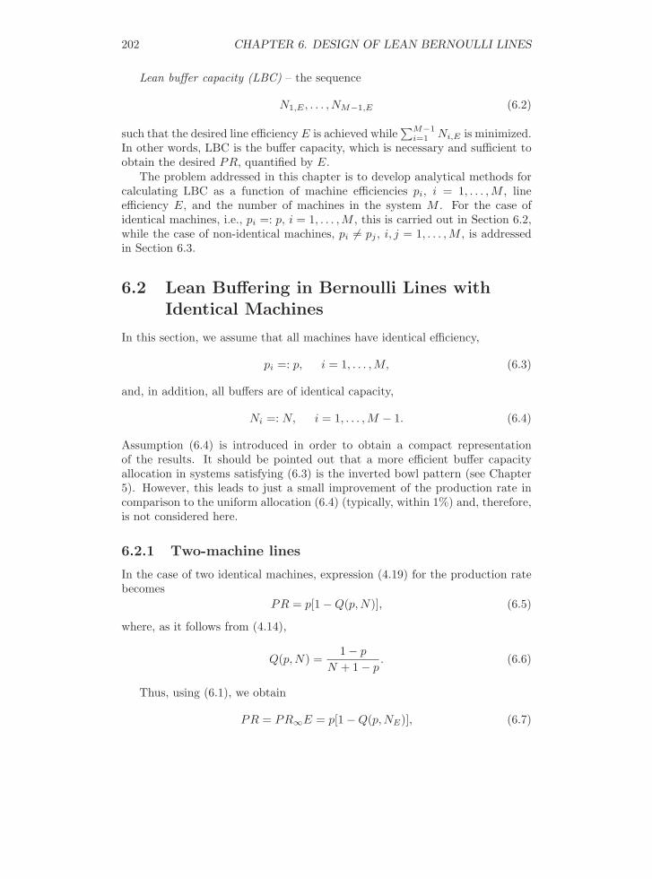
Figures 6.1(a) and 6.2(a) illustrate the behavior of the lean buffer capacityas a function of machine efficiency p and line efficiency E, respectively. Fromthese figures and expression (6.9), we observe:

(a) M = 2 (b) M = 3 (c) M = 10

Figure 6.1: Lean buffering as a function of machine efficiency

• For each E, LBC is a monotonically decreasing function of p, with apractically constant slope.

• For each p, LBC is a monotonically increasing function of E, exhibiting ahyperbolic behavior in 1− E.

• JIT operation is acceptable only if p’s are sufficiently large. For instance,if the desired line efficiency is 0.85, JIT can be used only if p > 0.83, whilefor E = 0.95, p must be larger than 0.95.

• In a practical range of p’s, e.g., 0.7 < p < 0.98, relatively small buffersare required to achieve a large E. For instance, N0.95 = 6 if p = 0.7; ifp = 0.9, N0.95 = 2.


(a) M = 2 (b) M = 3 (c) M = 10

Figure 6.2: Lean buffering as a function of line efficiency

6.2.2 Three-machine lines

For a three-machine line, using the aggregation procedure (4.30), the followingcan be derived:

Theorem 6.2 The lean buffer capacity in Bernoulli lines defined by con-ventions (a)-(e) of Subsection 4.2.1 with M = 3 and p1 = p2 = p3 =: p is givenby

NE(M = 3) =

ln{

1−√E1−E

}

ln{ (1−p)

√E

1−p√

E

}

. (6.10)

Proof: See Section 20.1.The behavior of this NE is illustrated in Figures 6.1(b) and 6.2(b). Obvi-

ously, for most values of p, the lean buffer capacity is increased, as comparedwith the case of M = 2, and the range of p’s where JIT is possible is decreased.For instance, if p = 0.95, JIT is acceptable for E < 0.91, while for p = 0.85 it isacceptable for E < 0.77.

6.2.3 M > 3-machine lines

Theorem 6.3 The lean buffer capacity in Bernoulli lines defined by con-ventions (a)-(e) of Subsection 4.2.1 with M > 3 and pi =: p, i = 1, . . . , M , isgiven by

NE(M > 3) =

ln{ 1−E−Q(pf

M−2, pbM−1, NM−2)

(1−E)(1−Q(pfM−2, pb

M−1, NM−2))

}

ln{ (1−p)(1−Q(pf

M−2, pbM−1, NM−2))

1−p(1−Q(pfM−2, pb

M−1, NM−2))

}

, (6.11)

where pfM−2 and pb

M−1 are the steady states of aggregation procedure (4.30) andfunction Q is defined by (4.14).

Proof: See Section 20.1.

6.2. LEAN BUFFERING FOR IDENTICAL MACHINES 205

Although a closed-form expression for Q cannot been derived (since N ’s areunknown and, therefore, pf

i and pbi cannot be calculated), its estimate can be

given as follows:

Q̂ = 1−E12 [1+( M−3

M−1 )M/4]+(

E12 [1+( M−3

M−1 )M/4]−E( M−2M−1 )

)exp

{− E

1M−1 − p

(1− E)(1/E)2E

}.

(6.12)Thus, an estimate of LBC for M > 3 is defined as

N̂E(M > 3) =

ln{

1−E−Q̂

(1−E)(1−Q̂)

}

ln{ (1−p)(1−Q̂)

1−p(1−Q̂)

}

, (6.13)

where Q̂ is given in (6.12).The accuracy of estimate (6.12), (6.13) has been evaluated numerically by

calculating the exact value of NE (using aggregation procedure (4.30) to evaluateQ) and comparing it with N̂E as follows:

∆E =N̂E −NE

NE· 100%. (6.14)

The values of ∆E have been calculated for p ∈ {0.85, 0.9, 0.95}, M ∈ {5, 10,15, 20, 25, 30}, and E ∈ {0.85, 0.9, 0.95}. It turned out that ∆E = 0 for allcombinations of these parameters except when [p = 0.85, M = 5, E = 0.85],where it is 50%. (Such a large error is due to the integer nature of NE andN̂E .) Thus, we conclude that in most cases N̂E provides a sufficiently accurateestimate of NE .

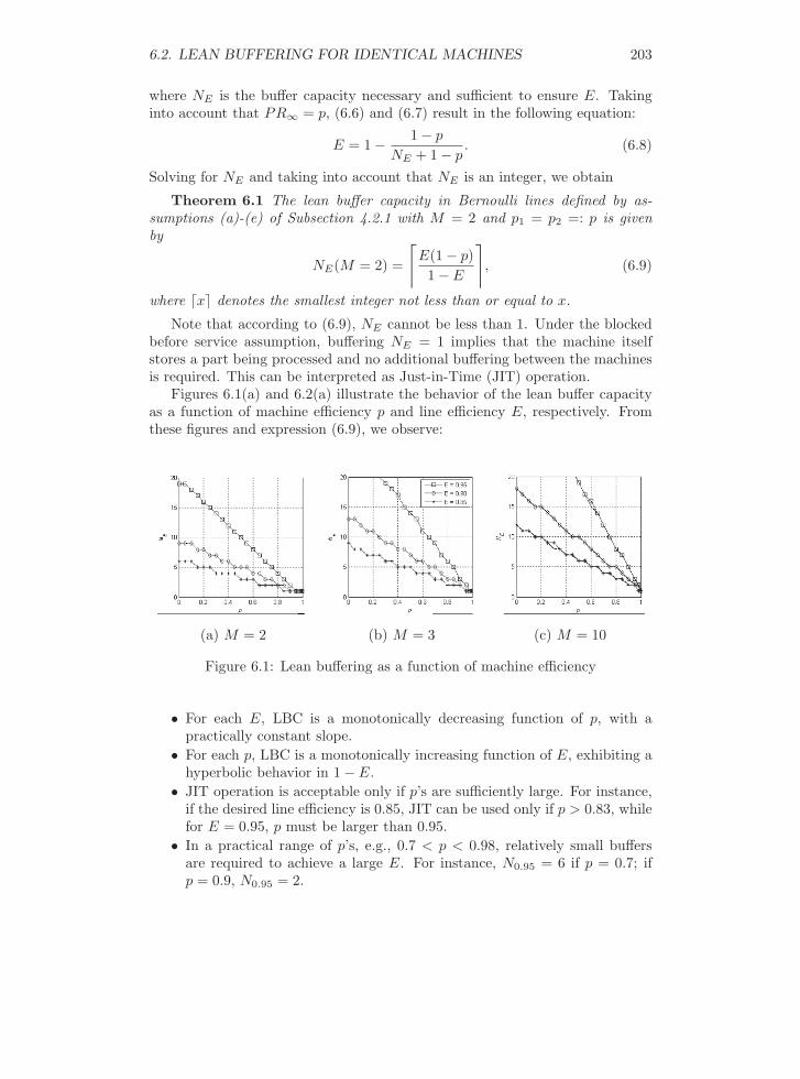
The behavior of N̂E for M = 10 is illustrated in Figures 6.1(c) and 6.2(c).Clearly, the buffer capacity is increased as compared to M = 3, and JIT opera-tion becomes unacceptable for all values of p and E considered.

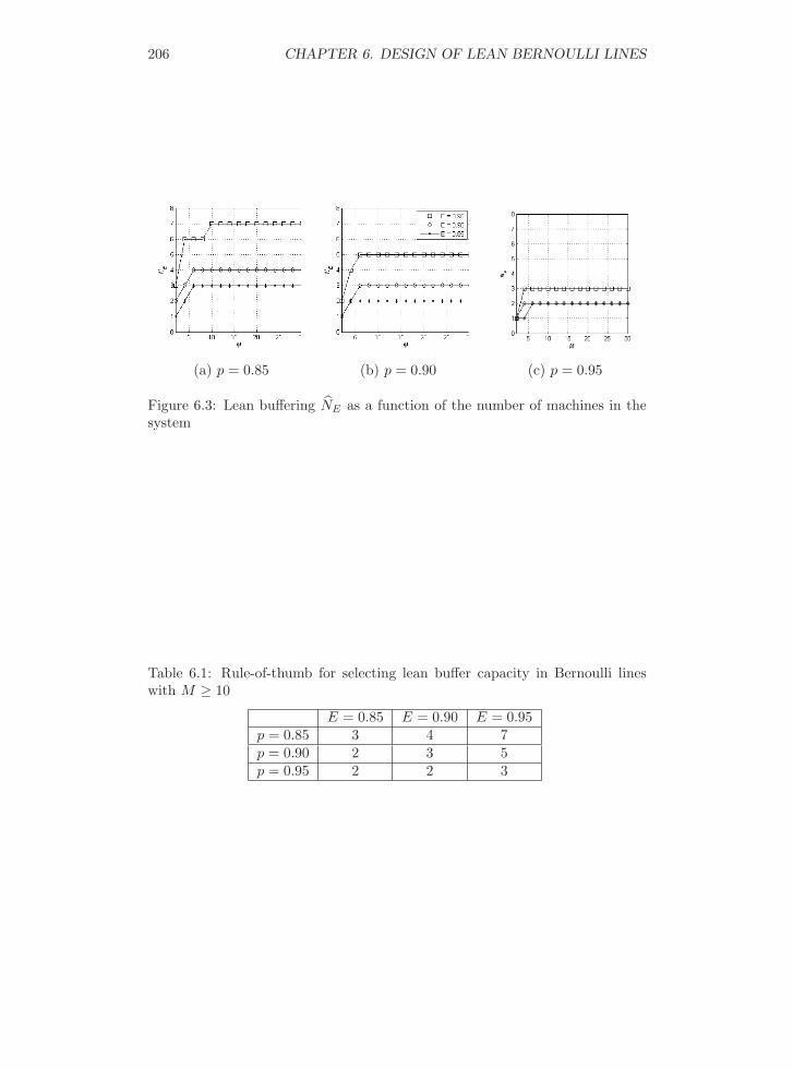
Using (6.12), (6.13), the behavior of lean buffering as a function of M canbe investigated. This is illustrated in Figure 6.3. Interestingly, and to a certaindegree unexpectedly, N̂E is constant for all M ≥ 10. This implies that the leanbuffering, appropriate for lines with 10 machines, is also appropriate for lineswith any larger number of machines. Based on this observation, the followingcan be formulated:

Rule-of-thumb for selecting lean buffering: In Bernoulli lines definedby conventions (a)-(e) of Subsection 4.2.1 with M ≥ 10, the capacity of the leanbuffering can be selected as shown in Table 6.1.

Interestingly, the diagonal elements of this “matrix” are all identical, imply-ing that buffer capacity 3 is necessary and sufficient to ensure line efficiency Eif p = E. The lower triangle of this matrix (p > E) has all elements smallerthan 3 and the upper (p < E) – larger than 3.


(a) p = 0.85 (b) p = 0.90 (c) p = 0.95

Figure 6.3: Lean buffering N̂E as a function of the number of machines in thesystem

Table 6.1: Rule-of-thumb for selecting lean buffer capacity in Bernoulli lineswith M ≥ 10

E = 0.85 E = 0.90 E = 0.95p = 0.85 3 4 7p = 0.90 2 3 5p = 0.95 2 2 3

6.3. LEAN BUFFERING FOR NON-IDENTICAL MACHINES 207

6.3 Lean Buffering in Serial Lines with Non-identical Bernoulli Machines

6.3.1 Two-machine lines

In the case of two-machine lines with non-identical machines, as it follows from(6.1) and (4.19), the equation that defines NE becomes

PR = PR∞E = p2[1−Q(p1, p2, NE)] = p2

[1− (1− p1)(1− α)

1− p1p2

αNE

], (6.15)

wherePR∞ = min(p1, p2) (6.16)

and

α =p1(1− p2)p2(1− p1)

. (6.17)

Solving (6.15) for NE , we obtain:

Theorem 6.4 The lean buffer capacity in Bernoulli lines defined by con-ventions (a)-(e) of Subsection 4.2.1 with M = 2 is given by

NE(p1, p2) =

ln{

p2p1

[p1−PR∞Ep2−PR∞E

]}

ln α

, (6.18)

where PR∞ and α are defined by (6.16) and (6.17), respectively.

Figure 6.4 illustrates the behavior of NE as a function of p1 for various valuesof p2 and E, while Figure 6.5 shows NE as a function of E for various p1 andp2. From these figures, we conclude:

0 0.2 0.4 0.6 0.8 10

1

2

3

4

5

6

p1

NE

0 0.2 0.4 0.6 0.8 10

1

2

3

4

5

6

p1

NE

p2 = 0.95

p2 = 0.85

p2 = 0.75

0 0.2 0.4 0.6 0.8 10

1

2

3

4

5

6

p1

NE

(a) E = 0.85 (b) E = 0.90 (c) E = 0.95

Figure 6.4: Lean buffering in two-machine lines as a function of the first machineefficiency


0.8 0.85 0.9 0.950

2

4

6

8

10

E

NE

0.8 0.85 0.9 0.950

2

4

6

8

10

E

NE

p2 = 0.95

p2 = 0.85

p2 = 0.75

0.8 0.85 0.9 0.950

2

4

6

8

10

E

NE

(a) p1 = 0.75 (b) p1 = 0.85 (c) p1 = 0.95

Figure 6.5: Lean buffering in two-machine lines as a function of line efficiency

• For p2 sufficiently large, JIT operation is acceptable for all values of p1

and E.• For small p2, JIT is acceptable only when p1 is sufficiently large. For

instance, if p2 = 0.75, JIT represents LBC only if p1 > 0.88 for E = 0.9and p1 > 0.94 for E > 0.95.

• The maximum of NE tends to take place when p1 = p2.

Intuitively, it is expected that the lean buffering in a line {p1, p2} is thesame as in the reversed line, i.e., {p2, p1}. It turns out that this is indeed trueas stated below.

Theorem 6.5 Lean buffer capacity has the property of reversibility, i.e.,

NE(p1, p2) = NE(p2, p1). (6.19)

Proof: See Section 20.1.

6.3.2 M > 2-machine lines

Exact formulas for LBC in the case of M > 2 are all but impossible to derive.Therefore, we limit our attention to estimates of Ni,E . These estimates areobtained based both on closed formulas (6.9)-(6.12), (6.18) and on recursivecalculations. Each of these approaches is described below.

Closed formula approaches: The following four methods have been inves-tigated:

I. Local pair-wise approach. Consider every pair of consecutive machines, mi

and mi+1, i = 1, . . . , M − 1, and select LBC using formula (6.18). Thisresults in the sequence of buffer capacities denoted as

N I1,E , . . . , N I

M−1,E .


II. Global pair-wise approach. It is based on applying formula (6.18) to allpossible pairs of machines (not necessarily consecutive) and then selectingthe capacity of each buffer equal to the largest buffer obtained by this pro-cedure. Clearly, this results in buffers of equal capacity, which is denotedas N II

E .

III. Local upper bound approach. Consider all pairs of consecutive machines,mi and mi+1, i = 1, . . . ,M − 1, substitute each of them by a two-machineline with identical machines defined by

p̂i := min{pi, pi+1}, i = 1, . . . , M − 1,

and select LBC using formula (6.9) with p = p̂i. This results in the se-quence of buffer capacities

N III1,E , . . . , N III

M−1,E .

IV. Global upper bound approach. Instead of the original line, consider a linewith all identical machines specified by

p̂ := min{p1, p2, . . . , pM}

and select the buffer capacity, denoted as N IVE , using expressions (6.12) and

(6.13). Due to the monotonicity of PR with respect to machine efficiencyand buffer capacity (see Chapter 4), this approach provides an upper boundof LBC:

Ni,E ≤ N IVE , i = 1, . . . ,M − 1.

If the desired line efficiency for two-machine lines, involved in approaches I -III, were selected as E, the resulting efficiency of the M -machine line would becertainly less than E. To avoid this, the efficiency, E′, of each of the two-machinelines is calculated as follows: For a given M -machine line, find the buffer capacityusing approach IV. Then consider a two-machine line with identical machines,where each machine is defined by p̂ = min{p1, . . . , pM}, and the buffer withthe capacity as found above. Finally, calculate the production rate and theefficiency of this two-machine line and use it as E′ in approaches I - III.

To analyze the performance of approaches I - IV, we consider 100, 000 linesformed by selecting M and pi randomly and equiprobably from the sets

M ∈ {4, 5, . . . , 30}, (6.20)

0.70 ≤ p ≤ 0.97. (6.21)

The desired efficiency for each of these lines is also selected randomly andequiprobably from the set

0.80 ≤ E ≤ 0.98. (6.22)


For each k-th line, thus formed, we calculate the vector of buffer capacities

Njk =

N j1,k

N j2,k

. . .

N jM−1,k

, k = 1, . . . , 100, 000, j = I, II, III, IV, (6.23)

using the four approaches introduced above. The subscripts of N ji,k represent

i-th buffer, i = 1, . . . , Mk − 1, of the k-th line, k = 1, 2, . . . , 100, 000; the super-script j = I, II, III, IV represents the approach used for this calculation. Inaddition, we calculate the production rate, PRj

k, and the efficiency, Ejk, using

expressions (4.30)-(4.36) and (6.1), respectively.The efficacy of approaches I - IV is characterized by the following two metrics:

1. The average buffer capacity per machine among all systems analyzed:

N jave =

1K

K∑

k=1

N jk (6.24)

where K = 100, 000 and

N jk =

1Mk − 1

Mk−1∑

i=1

N ji,k.

2. The percent of systems whose Ejk turns out to be less than the desired effi-

ciency Ek:

∆j =1K

K∑

k=1

Sg(Ek − Ejk) · 100%, (6.25)

where K = 100, 000 and

Sg(x) =

{1, x > 00, x ≤ 0.

The results are given in Table 6.2. Clearly, approach I leads to the small-est average buffer capacity but, unfortunately, almost always results in lineefficiency less than desired. Thus, a “local” selection of LBC (i.e., based onthe two machines surrounding the buffer) is, practically always, unacceptable.Approaches II and III provide line efficiency less than desired in only a smallfraction of cases and result in average buffer capacity 2 - 3 times larger than ap-proach I. Approach IV, as expected, always guarantees the desired performancebut requires the largest buffering.

To further differentiate between the four approaches, consider their per-formance as a function of M . To accomplish this, we formed 1000 lines foreach M ∈ {4, 6, 8, 10, 15, 20, 25, 30, 80} by selecting pi’s and E’s randomly and


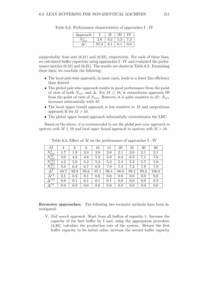
Table 6.2: Performance characteristics of approaches I - IV

Approach I II III IVN j

ave 2.0 6.2 5.3 7.2∆j 97.3 0.1 0.1 0.0

equiprobably from sets (6.21) and (6.22), respectively. For each of these lines,we calculated buffer capacities using approaches I - IV and evaluated the perfor-mance metrics (6.24) and (6.25). The results are shown in Table 6.3. Examiningthese data, we conclude the following:

• The local pair-wise approach, in most cases, leads to a lower line efficiencythan desired.

• The global pair-wise approach results in good performance from the pointof view of both Nave and ∆. For M ≤ 10, it outperforms approach IIIfrom the point of view of Nave. However, it is quite sensitive to M : Nave

increases substantially with M .• The local upper bound approach is less sensitive to M and outperforms

approach II for M > 10.• The global upper bound approach substantially overestimates the LBC.

Based on the above, it is recommended to use the global pair-wise approach insystems with M ≤ 10 and local upper bound approach in systems with M > 10.

Table 6.3: Effect of M on the performance of approaches I - IV

M 4 6 8 10 15 20 25 30 80N I

ave 1.7 1.9 2.0 2.0 2.0 2.1 2.0 2.1 2.1N II

ave 3.0 4.2 4.8 5.2 5.9 6.4 6.5 7.1 7.6N III

ave 4.2 5.0 5.2 5.2 5.2 5.4 5.3 5.7 5.6N IV

ave 5.0 6.3 6.7 6.8 7.0 7.4 7.3 7.9 7.9∆I 88.7 92.8 95.6 97.1 98.4 98.0 99.2 99.3 100.0∆II 3.1 0.3 0.1 0.0 0.0 0.0 0.0 0.0 0.0∆III 0.0 0.1 0.1 0.1 0.1 0.0 0.0 0.0 0.3∆IV 0.0 0.0 0.0 0.0 0.0 0.0 0.0 0.0 0.0

Recursive approaches: The following two recursive methods have been in-vestigated:

V. Full search approach. Start from all buffers of capacity 1. Increase thecapacity of the first buffer by 1 and, using the aggregation procedure(4.30), calculate the production rate of the system. Return the firstbuffer capacity to its initial value, increase the second buffer capacity


by 1, and calculate the resulting production rate. Repeat the sameprocedure for all buffers, determine the buffer that leads to the largestproduction rate, and permanently increase its capacity by 1. Repeat thesame procedure until the desired line efficiency is reached. This resultsin the sequence of buffer capacities

NV1,E , . . . , NV

M−1,E .

VI. Bottleneck-based approach. Consider a production line with buffer ca-pacity calculated according to approach I but rounded down in formula(6.18) rather than up. Although being relatively small, this buffering of-ten leads, as it follows from Tables 6.2 and 6.3, to line efficiency less thandesired. Therefore, to improve the line efficiency, increase the bufferingaccording to the following procedure: Using Bottleneck Indicator 5.1,identify the bottleneck machine (or, when applicable, primary bottle-neck machine) and increase the capacity of both buffers surrounding thismachine by 1. Repeat this procedure until the desired line efficiency isreached. This results in the sequence of buffer capacities denoted as

NV I1,E , . . . , NV I

M−1,E .

Clearly, approach V gives a smaller buffer capacity than approach VI. How-ever, the latter might require a shorter computation time. Therefore, in orderto compare V and VI, the computation time should be taken into account. Thisadditional performance metric is defined as the total computer time necessaryto carry out the calculation:

tj = tjend − tjstart, (6.26)

where tjstart and tjend, j ∈ {I, . . . , V I}, are the times (in seconds) of the begin-ning and the end of the computation.

Based on metrics (6.24), (6.25), and (6.26), we compared approaches I-VIusing the production systems generated by selecting pi’s randomly and equiprob-ably from set (6.21). The results are shown in Tables 6.4-6.6. Specifically, Tables6.4 and 6.5 present the results obtained using 5000 randomly generated 5- and10-machine lines, respectively, while Table 6.6 is based on the analysis of 2000randomly generated 15-machine lines. Examining these data, we conclude thefollowing:

• Full search approach, as expected, results in the smallest buffer capacityand the longest calculation time.

• Approaches II - IV, being based on closed-form expressions, are muchfaster than V (up to two orders of magnitude for long lines) but lead toaverage buffering 2 - 3 times larger than that of V.

• Approach VI provides a good tradeoff between the calculation time andbuffer capacity. In long lines, it is about 20 times faster than V and results


in average buffering almost the same as V (about 10% difference). Also, itis about 6 times slower than I - IV but gives buffering 2 - 3 times smallerthan II - IV.

Table 6.4: Performance characteristics of approaches I - VI in five-machine lines

(a) E = 0.80Approaches I II III IV V VI

N jave 1.5 2.2 2.4 2.9 1.4 1.5

∆j 27.8 0.0 0.0 0.2 0.0 0.0tj 8 8 8 8 59 28

(b) E = 0.85Approaches I II III IV V VI

N jave 1.7 2.7 3.0 3.6 1.7 1.8

∆j 36.0 0.0 0.0 0.2 0.0 0.0tj 8 8 8 8 91 38

(c) E = 0.90Approaches I II III IV V VI

N jave 2.2 3.6 4.2 5.0 2.0 2.3

∆j 33.8 0.0 0.0 0.0 0.0 0.0tj 6 6 6 6 91 27

(d) E = 0.95Approaches I II III IV V VI

N jave 3.2 6.0 7.9 9.5 2.8 3.3

∆j 25.5 0.0 0.0 0.0 0.0 0.0tj 6 6 6 6 150 29

Thus, if a recursive approach is to be used, the bottleneck-based one is rec-ommended.

Illustrative examples: To illustrate particular cases of lean buffering de-signed using approaches I - VI, we provide several examples.

Consider the four production lines with machines specified in Table 6.7 alongwith the desired line efficiency. The estimates of LBC for each of these lines,calculated using approaches I - VI, are shown in Tables 6.8 - 6.11, along withresulting line efficiency. These examples clearly indicate that:

• Approach VI is almost as good as the full search approach V.• Approach II in most cases outperforms approach III (since M = 5); how-

ever, it still leads to buffer capacity 2 - 3 times larger than approach V.


Table 6.5: Performance characteristics of approaches I - VI in 10-machine lines

(a) E ∈ [0.80, 0.89]Approaches I II III IV V VI

N jave 1.8 3.5 3.2 4.1 1.8 1.9

∆j 66.7 0.0 0.0 0.0 0.0 0.0tj 15 15 15 15 757 76

(b) E ∈ [0.89, 0.98]Approaches I II III IV V VI

N jave 3.2 8.0 8.2 10.6 2.7 3.2

∆j 48.5 0.0 0.0 0.0 0.0 0.0tj 26 26 26 26 2339 124

Table 6.6: Performance characteristics of approaches I - VI in 15-machine lines

(a) E ∈ [0.80, 0.89]Approaches I II III IV V VI

N jave 1.8 3.8 3.3 4.2 1.8 2.0

∆j 81.0 0.0 0.0 0.0 0.0 0.0tj 18 18 18 18 2452 107

(b) E ∈ [0.89, 0.98]Approaches I II III IV V VI

N jave 3.2 9.0 8.2 10.9 2.6 3.2

∆j 57.6 0.0 0.0 0.0 0.0 0.0tj 24 24 24 24 5837 138

Table 6.7: Machine parameters and desired line efficiencies

Line m1 m2 m3 m4 m5 E1 0.78 0.88 0.75 0.91 0.83 0.802 0.79 0.84 0.85 0.94 0.76 0.853 0.72 0.85 0.74 0.82 0.84 0.904 0.77 0.87 0.90 0.90 0.72 0.95


Table 6.8: LBC estimates and resulting efficiency for Line 1 (desired E = 0.80)

Buffer bj1 bj

2 bj3 bj

4 Ej

Desired 0.80N I

i 1 1 1 1 0.71N II

i 2 2 2 2 0.90N III

i 3 3 3 2 0.96N IV

i 3 3 3 3 0.96NV

i 1 2 2 1 0.83NV I

i 1 2 2 1 0.83


Buffer bj1 bj

2 bj3 bj

4 Ej

Desired 0.85N I

i 2 2 1 1 0.84N II

i 3 3 3 3 0.99N III

i 3 2 2 3 0.96N IV

i 3 3 3 3 0.99NV

i 1 2 2 1 0.85NV I

i 1 2 2 1 0.85


Buffer bj1 bj

2 bj3 bj

4 Ej

Desired 0.90N I

i 2 2 3 3 0.90N II

i 4 4 4 4 0.97N III

i 5 5 5 4 0.99N IV

i 5 5 5 5 0.99NV

i 2 3 2 2 0.90NV I

i 2 3 3 2 0.92


Buffer bj1 bj

2 bj3 bj

4 Ej

Desired 0.95N I

i 3 3 4 2 0.98N II

i 5 5 5 5 1.00N III

i 9 5 4 10 1.00N IV

i 10 10 10 10 1.00NV

i 2 2 2 2 0.96NV I

i 2 2 3 2 0.97


PSE Toolbox: The six methods of lean buffering calculation for Bernoullilines are implemented in the Lean Buffer Design function of the toolbox. Fora description and illustration of these tools, see Subsections 19.6.1 and 19.6.2.

6.4 Case Studies

6.4.1 Automotive ignition coil processing system

The Bernoulli model of this system is given in Figure 3.31 (for Periods 1 and2). Below, its lean buffering is evaluated using the model for Period 2 (since itcorresponds to system conditions during and after this case study).

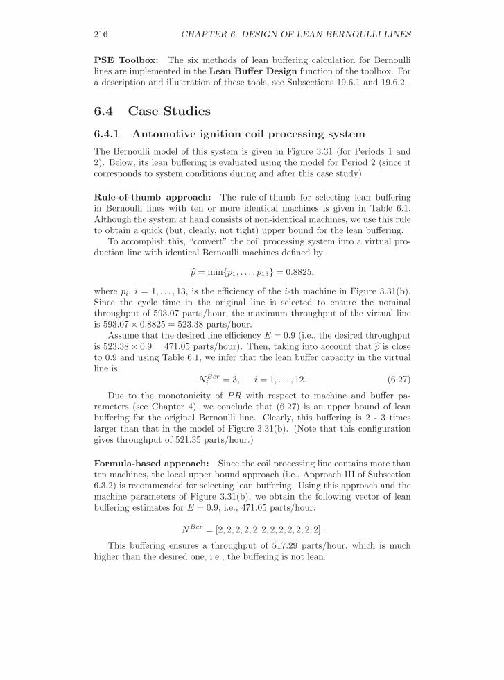
Rule-of-thumb approach: The rule-of-thumb for selecting lean bufferingin Bernoulli lines with ten or more identical machines is given in Table 6.1.Although the system at hand consists of non-identical machines, we use this ruleto obtain a quick (but, clearly, not tight) upper bound for the lean buffering.

To accomplish this, “convert” the coil processing system into a virtual pro-duction line with identical Bernoulli machines defined by

p̂ = min{p1, . . . , p13} = 0.8825,

where pi, i = 1, . . . , 13, is the efficiency of the i-th machine in Figure 3.31(b).Since the cycle time in the original line is selected to ensure the nominalthroughput of 593.07 parts/hour, the maximum throughput of the virtual lineis 593.07× 0.8825 = 523.38 parts/hour.

Assume that the desired line efficiency E = 0.9 (i.e., the desired throughputis 523.38× 0.9 = 471.05 parts/hour). Then, taking into account that p̂ is closeto 0.9 and using Table 6.1, we infer that the lean buffer capacity in the virtualline is

NBeri = 3, i = 1, . . . , 12. (6.27)

Due to the monotonicity of PR with respect to machine and buffer pa-rameters (see Chapter 4), we conclude that (6.27) is an upper bound of leanbuffering for the original Bernoulli line. Clearly, this buffering is 2 - 3 timeslarger than that in the model of Figure 3.31(b). (Note that this configurationgives throughput of 521.35 parts/hour.)

Formula-based approach: Since the coil processing line contains more thanten machines, the local upper bound approach (i.e., Approach III of Subsection6.3.2) is recommended for selecting lean buffering. Using this approach and themachine parameters of Figure 3.31(b), we obtain the following vector of leanbuffering estimates for E = 0.9, i.e., 471.05 parts/hour:

NBer = [2, 2, 2, 2, 2, 2, 2, 2, 2, 2, 2, 2].

This buffering ensures a throughput of 517.29 parts/hour, which is muchhigher than the desired one, i.e., the buffering is not lean.

6.4. CASE STUDIES 217

Recursive approach: Applying the bottleneck-based approach (i.e., approachVI of Subsection 6.3.2) with E = 0.9, we obtain a tighter estimate:

NBer = [1, 1, 1, 1, 1, 1, 2, 2, 1, 1, 1, 1].

Finally, using the full search approach, we arrive at a still tighter estimate:

NBer = [1, 1, 1, 1, 1, 1, 1, 2, 1, 1, 1, 1],

and this buffering leads to the line efficiency E = 0.923, i.e., the throughput of483.13 parts/hour.

6.4.2 Automotive paint shop production system

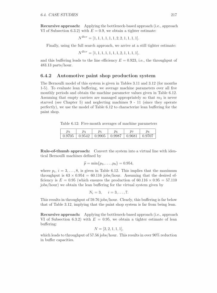
The Bernoulli model of this system is given in Tables 3.11 and 3.12 (for months1-5). To evaluate lean buffering, we average machine parameters over all fivemonthly periods and obtain the machine parameter values given in Table 6.12.Assuming that empty carriers are managed appropriately so that m3 is neverstarved (see Chapter 5) and neglecting machines 9 - 11 (since they operateperfectly), we use the model of Table 6.12 to characterize lean buffering for thepaint shop.

Table 6.12: Five-month averages of machine parameters

p3 p4 p5 p6 p7 p8

0.9705 0.9542 0.9905 0.9987 0.9681 0.9707

Rule-of-thumb approach: Convert the system into a virtual line with iden-tical Bernoulli machines defined by

p̂ = min{p3, . . . , p8} = 0.954,

where pi, i = 3, . . . , 8, is given in Table 6.12. This implies that the maximumthroughput is 63 × 0.954 = 60.116 jobs/hour. Assuming that the desired ef-ficiency is E = 0.95 (which ensures the production of 60.116 × 0.95 = 57.110jobs/hour) we obtain the lean buffering for the virtual system given by

Ni = 3, i = 3, . . . , 7.

This results in throughput of 59.76 jobs/hour. Clearly, this buffering is far belowthat of Table 3.12, implying that the paint shop system is far from being lean.

Recursive approach: Applying the bottleneck-based approach (i.e., approachVI of Subsection 6.3.2) with E = 0.95, we obtain a tighter estimate of leanbuffering:

N = [2, 2, 1, 1, 1],

which leads to throughput of 57.56 jobs/hour. This results in over 90% reductionin buffer capacities.


6.5 Summary

• Lean buffer capacity (LBC) is the smallest buffering necessary and suffi-cient to ensure the desired efficiency of a production line. Thus, LBC isthe “just-right” rather than “just-in-time” buffering.

• Lean buffer capacity in serial lines with identical Bernoulli machines can beevaluated using closed-form expressions (6.9)-(6.13) or the rule-of-thumbgiven in Table 6.1.

• In the case of non-identical machines, a closed formula is available onlyfor two-machine lines (6.18).

• For longer lines, estimates of lean buffer capacity can be obtained usingeither closed-form expressions or recursive calculations.

• If closed formulas are used, the global pair-wise approach and the localupper bound approach are recommended when M ≤ 10 and M > 10,respectively.

• If recursive calculations are used, the bottleneck-based approach is recom-mended.

6.6 Problems

Problem 6.1 Consider a Bernoulli serial line with two identical machines.Assume that it operates under the assumption of symmetric blocking describedin Problem 4.5.

(a) Derive the formula for lean buffer capacity in such a system.(b) Plot the lean buffer capacity as a function of machine efficiency.(c) Plot the lean buffer capacity as a function of line efficiency.(d) Does the symmetric blocking require larger or smaller lean buffering than

that defined by the blocked before service assumption (see Subsection 6.2.1)?

Problem 6.2 Consider the two-machine Bernoulli serial line with defectiveparts produced as described in Problem 4.4.

(a) Derive the formula for lean buffer capacity in such a system.(b) Plot the lean buffer capacity as a function of machine efficiency.(c) Plot the lean buffer capacity as a function of line efficiency.(d) Compare the resulting graphs with those obtained in Subsection 6.3.1 and

comment on the effect of the defectives on the lean buffer capacity.

Problem 6.3 Investigate the precision of the rule-of-thumb given in Table6.1. Specifically, consider the Bernoulli serial line with 15 identical machineshaving p = 0.87. Assume that the desired line efficiency is 0.93.

(a) Using expressions (6.12) and (6.13), calculate NE .

6.7. ANNOTATED BIBLIOGRAPHY 219

(b) Using the rule-of-thumb, determine an estimate of the lean buffer capacityfor this system.

(c) Compare the two results and comment on the applicability of the rule-of-thumb for p and E, which are not included in Table 6.1.

Problem 6.4 Consider the ignition device production line of Problem 3.3.

(a) Using any approach of Section 6.3, design the lean buffering for this systemwith E = 0.90.

(b) Using the same approach as in (a), design the lean buffering for this systemwith E = 0.97.

(c) Compare the two results and recommend which line efficiency should beused for practical implementation.

Problem 6.5 Consider the five-machine serial line of Problem 3.4. Assumethat the desired line efficiency is 0.97. Using the Bernoulli model of this line:

(a) Determine the estimate of the lean buffer capacity using the global upperbound approach of Subsection 6.3.2.

(b) Determine the estimate of the lean buffer capacity using the bottleneck-based approach.

(c) Compare the two results and state which of these approaches is preferable(from all points of view you find important).

Problem 6.6 Consider a production line with p = [0.88, 0.95, 0.9, 0.92]. Se-lect the lean buffering capacity for E = 0.95 using the following approaches:

(a) Global pair-wise approach.(b) Local upper bound approach.(c) Bottleneck-based recursive approach.(d) Full search recursive approach.

Compare the results and comment on the advantages and disadvantages of eachmethod.

6.7 Annotated Bibliography

The quantitative notion of lean buffering has been introduced and analyzed in

[6.1] E. Enginarlar, J. Li and S.M. Meerkov, “How Lean Can Lean Buffers Be?”IIE Transactions, vol. 37, pp. 333-342, 2005.

The lean buffering in Bernoulli lines, has been investigated in

[6.2] A.B. Hu and S.M. Meerkov, “Lean Buffering in Serial Production Lineswith Bernoulli Machines,” Mathematical Problems in Engineering, vol.2006, Article ID 17105, 2006.


It is the basis for the material of this chapter.Additional results on lean buffering (for the exponential and non-exponential

reliability models) can be found in

[6.3] E. Enginarlar, J. Li and S.M. Meerkov, “Lean Buffering in Serial Produc-tion Lines with Non-exponential Machines,” OR Spectrum, vol. 27, pp.195-219, 2005.

[6.4] S.-Y. Chiang, A.B. Hu and S.M. Meerkov, “Lean Buffering in Serial Pro-duction Lines with Non-identical Exponential Machines,” IEEE Transac-tions on Automation Science and Engineering, vol. 5, pp. 298-306, 2008.

design of lean bernoulli lines · design of lean bernoulli lines motivation: designers of...

Documents