design of wireless physiological measurement systems for

I

MÉMOIRE

PRÉSENTÉ À

L’UNIVERSITÉ DU QUÉBEC À CHICOUTIMI

COMME EXIGENCE PARTIELLE

DE LA MAÎTRISE EN INGÉNIERIE

By

Hongfei Cao

Design of Wireless Physiological Measurement Systems for

Patients Affected by COPD

September 2017

II

Résumé

La maladie pulmonaire obstructive chronique (MPOC) est un trouble respiratoire chronique qui

affecte un grand nombre d’adultes au Canada. Les patients affectés par cette maladie tendent à

être moins actifs et risquent de perdre leur capacité fonctionnelle. Par conséquent, il serait

important pour eux de faire de l'activité physique régulièrement. En raison de certaines

contraintes, tels que le froid, l’espace d’entraînement limité et l'isolement géographique, la

pratique d'activité physique n'est pas toujours possible. Dans ce cas, un programme d’exercices

de réhabilitation effectué à domicile pourrait être une bonne solution. Afin d’aider ces patients à

demeurer actifs, des chercheurs mettent au point une infrastructure matérielle et logicielle afin

d’entraîner ces patients à distance par un lien internet. Puisque la MPOC est une maladie qui

peut être mortelle, trois paramètres physiologiques principaux (fréquence respiratoire, la

saturation en oxygène et le rythme cardiaque) doivent être surveillés en temps réel pendant

l'entraînement pour assurer la sécurité des patients. L’objectif de ce projet de maîtrise est de

développer deux instruments sans fil pour mesurer ces paramètres physiologiques : une ceinture

de détection du rythme respiratoire et une oxymètre de pouls. Des essais ont été effectués pour

évaluer la performance de ces instruments. Les résultats des essais ont montré que ces

instruments fonctionnent tel que prévu. À l’aide de ces instruments, les patients MPOC

pourraient être actifs pendant toute l’année et ainsi maintenir leurs capacités fonctionnelles.

III

Abstract

Chronic obstructive pulmonary disease (COPD) is a chronic respiratory disorder that affects

many adults in Canada. Patients affected by such a condition tend to become less active and are

at risk of losing functional capacity. Therefore, it is important for them to exercise regularly

throughout the year. However, there are some restricting situations, such as cold weather, limited

training space and long distance from training centers that may prevent the regular practice of

exercise. In those cases, a rehabilitation exercise program at patients’ homes may be a good

option. To help these patients remain active, researchers are developing a hardware/software

infrastructure for training remote patients via the internet. Since COPD is a disease that can be

deadly, 3 key physiological parameters need to be monitored to ensure the safety of the patients:

respiratory rate, oxygen saturation and heart rate. The objective of this master’s project was to

develop two wireless instruments to measure physiological parameters: a respiratory sensor belt

and a pulse oximeter. A series of experiments were carried out to evaluate the performance of the

designed instruments. The test results showed these instruments meet the design requirements

and are able be used to monitor the COPD patients. This will help patients with COPD stay

active all year and ultimately, help maintain their functional capacity and their quality of life.

IV

Table of Contents

Résumé ............................................................................................................................................ II

Abstract ......................................................................................................................................... III

List of Figures ............................................................................................................................... VI

List of Tables ............................................................................................................................. VIII

List of Symbols and Abbreviations............................................................................................... IX

Acknowledgements ....................................................................................................................... XI

1. Introduction ................................................................................................................................. 1

1.1 Background ........................................................................................................................... 1

1.2 Objectives and Scope of the Project ...................................................................................... 1

2. Literature Review........................................................................................................................ 3

2.1 Different Methods of Measuring the Respiratory Rate ......................................................... 3

2.2 Oxygen Saturation and Major Analytical Methods............................................................... 5

2.3 Pulse Oximetry Theory Review and Calibration Approach. ................................................. 6

2.3.1 Pulse Oximetry Theory Review ..................................................................................... 6

2.3.2 Limitations of the Beer-Lambert Model and Calibration Approach of Commercial

Pulse Oximeter ........................................................................................................................ 8

2.3.3 Pulse Oximetry Signals for Heart Rate Measurement .................................................... 9

2.3.4 Overview of Commercial Pulse Oximeters .................................................................. 10

3. Methodology and Design Procedure ......................................................................................... 11

3.1 Methodology ....................................................................................................................... 11

3.2 Initial Instrument Design for Respiratory Rate Measurement ............................................ 12

3.2.1 Instrument Design Requirements ................................................................................. 12

3.2.2 Instrument Design Method ........................................................................................... 12

3.2.3 Respiratory Sensor Belt Development ......................................................................... 13

3.2.4 Microcontroller and Hardware Design ......................................................................... 13

3.2.5 Software Design ........................................................................................................... 16

3.3 Initial Design of the Pulse Oximeter ................................................................................... 18

3.3.1 Hardware Design and Components Selection .............................................................. 19

3.3.2 Algorithm and Software Implementation. .................................................................... 36

4. Experiments and Results ........................................................................................................... 44

4.1 Respiration Rate Monitor System Test. .............................................................................. 44

V

4.1.1 Material and Method .................................................................................................... 44

4.1.2 Testing Results ............................................................................................................. 45

4.2 Pulse Oximeter Test ............................................................................................................ 47

4.2.1 Material and Method .................................................................................................... 47

4.2.2 Testing Results ............................................................................................................. 49

5. Conclusion and Future Work .................................................................................................... 55

References ..................................................................................................................................... 57

Appendix A Beer's Law and Light Transmittance ........................................................................ 59

Appendix B Beer-Lambert Model in Pulse Oximetry .................................................................. 62

VI

List of Figures

Figure 2.1 A Two-Electrode Circuit Model .................................................................................... 4

Figure 2.2 Extinction Spectra of O2Hb and HHb ........................................................................... 6

Figure 2.3 Sample Calibration Curve ............................................................................................. 9

Figure 2.4 Pulsatile Signal while IR or Red light is Transmitted through the Tissue. ................. 10

Figure 3.1 Wireless Instruments Needed for Remote Monitoring of COPD Patients. ................. 11

Figure 3.2 Real-time Respiration Rate Monitor System Diagram. ............................................... 12

Figure 3.3 Conductive Rubber Cord. ............................................................................................ 13

Figure 3.4 Conductive Rubber Cord Fixed on an Elastic Band. ................................................... 13

Figure 3.5 Arduino Micro. ............................................................................................................ 14

Figure 3.6 The Sensor Voltage Divider Circuit. ........................................................................... 14

Figure 3.7 Schematic of the Hardware Connection. ..................................................................... 15

Figure 3.8 PCB of the Designed Circuit ....................................................................................... 16

Figure 3.9 XBee Wireless Module................................................................................................ 16

Figure 3.10 Program Flow Chart. ................................................................................................. 17

Figure 3.11 Pulse Oximeter Design .............................................................................................. 19

Figure 3.12 Arduino UNO ............................................................................................................ 20

Figure 3.13 Comparison between Transmittance and Reflectance Probes in Pulse Oximetry ..... 21

Figure 3.14 Finger Clip Probe along with its Interface Connector Employed in the Design. ...... 21

Figure 3.15 Schematic of Finger Probe. ....................................................................................... 22

Figure 3.16 Schematic of Designed LED Drive Circuit. .............................................................. 23

Figure 3.17 Red LED Current Control Circuit. ............................................................................ 24

Figure 3.18 IR LED Current Control Circuit. ............................................................................... 25

Figure 3.19 DAC Schematic. ........................................................................................................ 27

Figure 3.20 Current to Voltage Converter in the Circuit. ............................................................. 28

Figure 3.21 Bode Plot of the First Active Filter. .......................................................................... 29

Figure 3.22 Output Signal of TIA ................................................................................................. 30

Figure 3.23 Bode Plot of an Ideal Passive Band Pass Filter. ........................................................ 31

Figure 3.24 Schematic of the Designed Band Pass Filter. ............................................................ 32

Figure 3.25 Bode Plot of the Designed Band Pass Filter. ............................................................. 32

VII

Figure 3.26 Signal at the Output of Band Pass Filter. .................................................................. 33

Figure 3.27 Active Low Pass Filter. ............................................................................................. 34

Figure 3.28 Voltage Divider Circuit ............................................................................................. 35

Figure 3.29 Output of the Last Filter as a Response to the IR LED. ............................................ 35

Figure 3.30 An IR-light Signal Plot Graph of the Testing Participant. ........................................ 36

Figure 3.31 A Red-Light Signal Plot Graph of the Testing Participant. ....................................... 37

Figure 3.32 Algorithm 1 on IBI, AC and DC values Calculation. ............................................... 39

Figure 3.33 Algorithm 2 on Heart Rate Calculation. .................................................................... 40

Figure 3.34 Buffer Shifting for IBI Values. .................................................................................. 41

Figure 3.35 Flow Chart of the Program ........................................................................................ 42

Figure 3.36 Pulse Signals on Oscilloscope during LED Switching.............................................. 43

Figure 4.1 The Designed Respiration Monitor System during the Test ....................................... 44

Figure 4.2 Elapsed time (milliseconds) and the Corresponding Real-time Respiration Rate

(breaths per minute) Received from Arduino At Rest State. ........................................................ 45

Figure 4.3 Elapsed Time (milliseconds) and the Corresponding Real-time Respiration Rate

(breaths per minute) Received from Arduino at A Rapid Respiration Rate. ................................ 46

Figure 4.4 Signal Waveforms on Oscilloscope in the Rapid Respiration Test. ............................ 46

Figure 4.5 Comparison of Real-time Test Results between the Prototype and MD300c ............. 48

Figure 4.6 Stationary Bike Used in the Test. ................................................................................ 49

Figure 4.7 Comparison of Real-time Heart Rate at Rest .............................................................. 51

Figure 4.8 Comparison of Real-Time Heart Rate after Prescribed Exercises .............................. 51

Figure 4.9 Comparison of SpO2 Measurement between the Prototype and MD300c.................. 52

Figure 4.10 SpO2 of Participant 1 ................................................................................................ 53

Figure 4.11 SpO2 of Participant 2. ............................................................................................... 54

VIII

List of Tables

Table 3.1 Functionality of the ADG884 Input Logic Signal. ....................................................... 24

Table 4.1 Average Results and Percentage of Error for Heart Rate and SpO2. ........................... 50

IX

List of Symbols and Abbreviations

COPD Chronic Obstructive Pulmonary Disease

CHUL Centre Hospitalier de l’Université Laval

EMFit Electromechanical Film

ADC Analog to Digital Converter

DAC Digital to Analog Converter

PEP Pyroelectric Polymer

O2Hb Oxyhemoglobin

HHb Deoxyhemoglobin

SO2 Oxygen Saturation

pH Power of Hydrogen

PaO2 Partial Pressures of Oxygen

SpO2 Arterial Oxygen Saturation

IR Infrared

LED Light-Emitting Diode

PD Photodiode

AC Alternating Current

DC Direct Current

PCB Print Circuit Board

PPG Plethysmography

UART Universal Asynchronous Receiver/Transmitter

SPDT Single-pole, Double-throw

EEPROM Electrically Erasable Programmable Read-only Memory

I2C Inter-integrated Circuit

SCL Serial Clock Line

SDA Serial Data Line

TIA Transimpedance Amplifier

BPM Beats per Minute

X

IBI Inter Beat Interval

ISR Interrupt Service Routine

XI

Acknowledgements

I would like to thank Prof. Hung Tien Bui, my director, for his guidance, encouragement,

support, motivation and patience in my study. Special thanks to Prof. Mario Leone, my co-

director for his patience and guidance. I am particularly grateful for all your help during my

studies.

I would like to thank my evaluation committee members for all their guidance through this

process; your ideas and feedback have been absolutely invaluable.

I would like to thank all my friends for their support and friendship. I would like to thank my

family for their continuing support.

1

1. Introduction

1.1 Background

Chronic obstructive pulmonary disease (COPD) is a respiratory disorder typically characterized

by chronic obstruction of lung airflow that interferes with normal breathing and is not fully

reversible [1]. It is a common lung disease in Canada affecting at least 700,000 adults and is now

the fourth leading cause of death [2]. People with COPD are likely to present symptoms such as

shortness of breath, persistent cough, chest tightness and lack of energy. As COPD sufferers

often find the normal daily routines (climbing stairs, shopping, housework, etc.) an uphill

struggle, it often leads to a progressively inactive lifestyle. This will cause a vicious cycle that

causes health to deteriorate in these patients. Proper rehabilitation training programs have been

shown to have beneficial effects on COPD patients [3]. A prescribed exercise program enables

COPD patients to increase physical capacity and day to day autonomy. Due to some restricting

situations, such as cold weather, limited training space and long distance from training centers, a

rehabilitation exercise program designed to be performed at patients’ homes may be a good

option. Since COPD is a disease that can be deadly, several factors in the training process, such

as improper training intensity, duration and frequency may lead the patients to a potentially

dangerous situation. Therefore, the patients’ safety must be considered during the training

program. A real-time monitored training program that assesses key physiological parameters of

the patients could be an effective solution. A training expert could then ensure the patients’

safety by monitoring the following physiological parameters: respiratory rate, oxygen saturation

and heart rate.

1.2 Objectives and Scope of the Project

Recent advances in technology have helped improve the speed and quality of communications

media. More particularly, the speed of internet connections has increased dramatically, thus

allowing real time transmission of audio and video streams. This has paved the way for

applications such as video conferences where individuals from any location can discuss while

also establishing visual contact. More recently, certain research groups have proposed it as a tool

for medical/health supervision. This would help the population quickly gain access to health

2

professionals even when they are in remote locations or when travelling to the clinic is not a

viable option.

For this reason, researchers at Université du Québec à Chicoutimi (UQAC) and at the Centre

Hospitalier de l’Université Laval (CHUL) are developing a hardware/software infrastructure for

training of remote patients affected by COPD. With the help of the infrastructure, a health

specialist will monitor several COPD patients performing exercises over an internet connection

and ensure that the movements are performed correctly and that the exercise intensity remains

within prescribed limits. In order to do so, they require a visual connection as well as real-time

measurements of physiological signals.

The objective of this master’s project was to develop the instruments required to measure the

three aforementioned parameters (respiratory rate, heart rate and oxygen saturation). These

instruments needed to be small, wireless, low-cost and accurate.

3

2. Literature Review

In this chapter, we present a detailed analysis of the existing measurement methods related to the

desired physiological parameters as well as existing implementations.

2.1 Different Methods of Measuring the Respiratory Rate

Respiratory parameters are important for research in healthcare monitoring. The respiratory rate,

which is defined as the number of breaths per minute, is an essential physiological parameter in

abnormal breathing diagnosis. Therefore, many systems have been developed for respiratory rate

measurements. These systems are mainly based on three kinds of methods: thoracic/abdominal

expansion measurement, impedance pneumography and airflow breath measurement.

The first method is based on the fact that the thorax and the abdomen expand and retract with

every breath. By measuring the frequency of this expansion/retraction, it is possible to measure

the rate at which a person breathes. Over the years, researchers have proposed multiple methods

to measure this expansion/retraction. Some researchers have used a mercury filled elastic strain-

gauge (Silastic™), whose resistance is sensitive to changes in length. By wrapping this elastic

around the torso, the breathing rate can be measured. However, as mercury is a hazardous

material, mercury-filled strain gauges are rarely used today. In recent years, wearable sensor-

based health monitoring devices, such as BioHarness™ 3 Chest Strap and Hexoskin™ smart

shirt have appeared on the market. While they could provide accurate respiratory rate, their

relative high costs make them less appropriate for monitoring of a large number of patients.

Similarly, Tuomas Reinvuo et al. from the University of Oulu have created a sensor belt with a

high-resolution accelerometer and an electromechanical film (EMFit) pressure sensor to measure

respiratory rate[4]. Results show that the sensor belt is a portable and accurate tool for

respiratory rate measurement. However, the system is only suitable for the immobile testing.

The second technique, known as impedance pneumography, is based on the fact that air causes a

change in electrical impedance in the lungs. Therefore, by measuring the rate of change in

impedance in the lungs, it would be possible to determine the breathing rate. To use this

approach, either two or four electrodes are attached to the chest. The impedance in the thorax can

4

be divided into two components: a relatively constant baseline impedance R𝐵 and a varying

respirative impedance ∆R[5]. During inspiration, the increase in gas volume of the chest and the

expansion of the thorax cause ∆R to increase[6]. The relationship between the total

impedance(∆R+R𝐵) and the volume of air in the lungs is approximately linear[7]. If electrical

current was applied to the electrodes during the breathing process, the change in impedance (∆R)

will result in a change in voltage (∆V). To perform breathing rate measurement, a possible

approach is to inject a high-frequency AC current into the body through the electrodes. This ac

signal acts as a carrier signal that is amplitude-modulated by the change in voltage caused by

respiration (∆V). After demodulation and denoising with a low-pass filter, the output can then be

digitized by an analog to digital converter (ADC). The respiratory rate then could be calculated.

Figure 2.1 shows a typical two-electrode circuit model [7]. In this figure, Rp are the defibrillator

protection resistances within the cables that are in series with the electrode impedances

(𝑍Electrode) which consist of a 51-kΩ resistor and 47-nF capacitor in parallel [3].

Figure 2.1 A Two-Electrode Circuit Model

The third type of approach used in respiration measurement consists of measuring the air

exhaled. For this approach, it is customary to use a face mask to either measure the air

displacement or the change in temperature due to respiration. Dodds et al. proposed the use of a

pyroelectric polymer (PEP) film as a transducer for respiratory rate measuring[8]. The PEP film

is a material that generates a voltage when its temperature or pressure is changed (pyroelectric

effect). In their proposed system, the material is mounted to the internal surface of a standard

oxygen face mask. The voltage variation, caused by the change in temperature during respiration,

is sent to an ADC after signal processing. Results show that the PEP film is a low-cost and

5

reliable transducer for respiratory rate monitoring. The major disadvantage with this approach is

the use of a face mask which may cause discomfort in many participants and the need daily

maintenance for proper hygiene.

2.2 Oxygen Saturation and Major Analytical Methods

Oxygen transport is important in sustaining human life. Hemoglobin is a protein that is capable

of carrying and releasing molecular oxygen (𝑂2) in erythrocytes (red blood cells). Hemoglobins

can be divided into oxyhemoglobin ( 𝑂2𝐻𝑏 𝑜𝑟 𝐻𝑏𝑂2 ) and deoxyhemoglobin ( 𝐻𝐻𝑏 or 𝐻𝑏 ),

according to whether they are fully saturated with oxygen or not. Most of the hemoglobin in

human blood is either in the form of 𝑂2𝐻𝑏 or 𝑏 . For new born babies with certain respiratory

problems and patients under anesthesia, their blood oxygenation needs to be monitored since

they are unable to breathe on their own. It is important to determine whether they are absorbing

the necessary amount of oxygen supplied by ventilators. Similarly, for patients with certain

respiratory problems, such as COPD, oxygen absorption could fall to dangerously low levels.

Therefore, the assessment of oxygen saturation (S𝑂2)— a parameter that indicates the ratio of

the oxyhemoglobin over both oxy and deoxyhemoglobins, provides a valuable indictor in

respiration monitoring.

The following empirical equation is used to determine hemoglobin oxygen saturation, using

measured hemoglobin concentrations:

S𝑂2 =𝑐𝑂2𝐻𝑏

𝑐𝑂2𝐻𝑏+𝑐𝐻𝐻𝑏 （2.1）

A normal range of S𝑂2 for healthy adults，expressed as a percentage，is typically 94%–98%.

For patients who are not achieving the critical blood oxygen saturation level of 90%, proper

treatments may be required [9].

There are three major analytical methods used to measure oxygen saturation: arterial blood gas

analyzers, CO-oximetry and pulse oximetry [10]. The arterial blood gas analyzers calculate

estimated oxygen saturation in a blood sample based on empirical equations using power of

hydrogen (pH) and the partial pressures of oxygen (PaO2) values. The CO-oximetry measures

the absorption of hemoglobin derivatives from blood samples using multiple wavelengths of

6

light. While they are precise, the above two methods require blood samples and do not support

real-time monitoring and therefore, are not suitable for our project.

2.3 Pulse Oximetry Theory Review and Calibration Approach.

2.3.1 Pulse Oximetry Theory Review

Pulse oximetry is a noninvasive method of continuously assessing arterial oxygen saturation

(SpO2 or SaO2) and the pulse rate of a patient. It is widely prevalent in health care and is often

regarded as the fifth vital sign after body temperature, pulse rate, respiration rate and blood

pressure[11]. By measuring light absorption at a well-perfused body area (finger, ear lobe or

nasal alar) with two different wavelengths (red and infrared), it assesses the SpO2 and the pulse

rate.

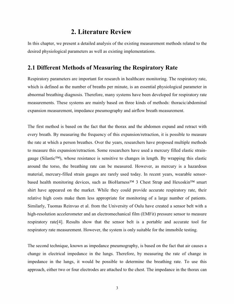
The general principle of pulse oximeters is explained as follows. According to the optical

properties of 𝑂2𝐻𝑏 and 𝐻𝐻𝑏 (Figure 2.2), the absorption of 𝑂2𝐻𝑏 and 𝐻𝐻𝑏 at red and near-

infrared (IR) light are significantly different. 𝐻𝐻𝑏 allows more IR light (940 nm) to pass and

absorbs more red light (660nm), while 𝑂2𝐻𝑏 behaves in the opposite way. This is in accordance

with the fact that well-oxygenated blood with higher concentration of 𝑂2𝐻𝑏 often appears redder

to the eye than poorly-oxygenated blood.

Figure 2.2 Extinction Spectra of O2Hb and HHb [12].

7

It is also important to note that the body tissues do not typically attenuate the optical signals at

these two wavelengths whereas yellow, green, blue, and far- IR light signals are significantly

absorbed by vascular tissues and water[13].

Based on the above difference in light absorption properties of 𝑂2𝐻𝑏 and 𝐻𝐻𝑏, a pulse oximeter

typically emits two wavelengths of light, red light at 660 nm and near- IR light at 940 nm from

two light-emitting diodes(LEDs). These lights will then transmit through the finger, ear lobe or

other body tissues and will be detected by a photodiode or photo detector (PD). The LEDs and

PD are commonly integrated together in a device called a probe in a pulse oximeter. The light

signal received on the PD is converted into an electrical signal. thus, the relative absorption of

red and IR light can be quantified.

If we assume the transmission of light through the arterial blood is influenced only by the

relative concentrations of 𝑂2𝐻𝑏 and 𝐻𝐻𝑏 and their absorption coefficients at the two

measurement wavelengths, the light intensity will decrease logarithmically with path length

according to the Beer−Lambert law[14] (see Appendix A). With these principles, the ratio of the

intensity of light transmitted at two different wavelengths could be expressed as follow:

R = log10 (𝐼1) / log10 (𝐼2) （2.2）

In Equation (2.2), 𝐼1 is the intensity of light with wavelength λ1 (660 nm) and 𝐼2 is the intensity

of light with wavelength λ2 (940nm).

Once the absorbance coefficients of 𝑂2𝐻𝑏 and 𝐻𝐻𝑏 at the two wavelengths are known, the

oxygen saturation can be obtained using the following equation:

SpO2 = (αr2*R - αr1) / [(αr2 – αo2) *R – (αr1 – αo1)]. （2.3）

Where:

• αr1 is the extinction coefficient of 𝐻𝐻𝑏 at λ1

• αr2 is the extinction coefficient of 𝐻𝐻𝑏 at λ2

• αo1 is the absorption coefficient of 𝑂2𝐻𝑏 at λ1

• αo2 is the absorption coefficient of 𝑂2𝐻𝑏 at λ2

8

• R is the ratio obtained from Equation (2.2)

• SpO2 is the arterial oxygen saturation

This SpO2 calculation principle is based on the Beer−Lambert model (see Appendix B).

2.3.2 Limitations of the Beer-Lambert Model and Calibration Approach of

Commercial Pulse Oximeter

In the Beer-Lambert model, the arterial blood is treated as a homogeneous absorbing medium. In

real situations, the absorbance of light is not simply proportional to the concentration of

hemoglobin or to the optical path length but are also dependent on scattering and multiple

scattering. This phenomenon can occur when light is refracted by a similar-sized object to the

wavelength of the light, as in the case of red/IR light having the same size wavelength as red

blood cells (approximately 7 µm in diameter). Scattering causes the deviation of a light beam

from its initial direction and therefore, highly increases light absorbance. In addition, light that is

scattered once will likely be scattered again by cells and therefore multiple scattering occurs[14].

Therefore, the Beer-Lambert model can’t be applied directly to the SpO2 calculation in pulse

oximetry. As the process of mathematically modeling the problem of light scattering for different

conditions is very complex, most commercial pulse oximeters use calibration curves from

empirical formulas to determine the SpO2. This method provides SpO2 values that are accurate

enough for clinical use.

Instead of calculating the standard R value using Equation (2.2), an approximation of the R value

is typically employed in pulse oximetry as the error is negligible (below 0.02%)[15].

R = (ACred /DCred)/ (ACIR / DCIR) (2.4)

In the equation, ACred and ACIR are the absorbance of pulsatile “alternating current” component

of the red and IR light. DCred and DCIR is the absorbance of non-pulsatile “direct current” (DC)

component of the red and IR light.

Therefore, R can be obtained from the AC/DC ratio of red and IR light signals. In the pulse

oximeter algorithm, the continuously calculated R value is used together with a look-up table

which is made up of empirical formulas to determine the SpO2. As an important part of the pulse

oximeter system, the look-up tables are usually based on calibration curves generated empirically

9

from measuring the R values of many healthy subjects with SpO2 levels altered from 100% to

approximately 70%[16]. The SpO2 of the healthy subjects is usually measured by a very

accurate method such as co-oximeter. Figure 2.3 shows a sample calibration curve.

Figure 2.3 Sample Calibration Curve.

Since generating a custom calibration curve is both time consuming and expensive, Equation

(2.5) is often suggested in the literature[14].

SpO2=110-25*R (2.5)

This equation is a linear approximation of an empirical calibration curve established by

measurements of a large group of healthy volunteers with SpO2 values generally greater than

70%. Therefore, it could be used to compute the SpO2 in our design.

2.3.3 Pulse Oximetry Signals for Heart Rate Measurement

In pulse oximetry, when the IR or red light is transmitted through the tissue, it produces a

pulsatile signal as shown in Figure 2.4 [17]. The signal varies with time in relation to the heart

beat. Therefore, the heart rate frequency of the individual can be extracted from the waveform.

10

Figure 2.4 Pulsatile Signal while IR or Red light is Transmitted through the Tissue.

2.3.4 Overview of Commercial Pulse Oximeters

With recent technological advancements and increasing interest in physiological measurements,

low-cost pulse oximeters have become widely available on the market. Wireless portable pulse

oximeters have also emerged, such as the health Air PO3 and the Massimo MAS-9809. In these

products, the measured SpO2 and heart rate are transferred to Apple iOS or Android devices with

their customer application programs via Bluetooth LE connectivity[18, 19]. These devices can be

very useful in typical situations. However, in this project, the wireless pulse oximeter is used

together with the wireless respiration belt to monitor the patient’s physiological parameters.

Hence, to synchronize the data, the pulse oximeter needs to be compatible with the already

designed wireless respiration belt. Unfortunately, the wireless communication standard used by

the commercial pulse oximeters on the market (Bluetooth LE) could not interface with the XBee

wireless module that was used in the designed respiration monitoring system[20]. Meanwhile,

designing a new pulse oximeter in the project could also pave the way for more integrated

measurements systems. For example, researchers have demonstrated the possibility of detecting

respiratory signals in plethysmograms obtained from pulse oximeters[21]. With a modified pulse

oximeter, it would be possible to measure the three-aforementioned key physiological parameters

using a single piece of equipment. Therefore, it was deemed important to design a pulse oximeter

for this project.

11

3. Methodology and Design Procedure

3.1 Methodology

For the purpose of the master’s project, two wireless instruments were developed to monitor 3

key physiological parameters, respiratory rate, oxygen saturation and heart rate. This helps

ensure the safety of the COPD patients during their exercise program. Figure 3.1 shows the

principle of our wireless system when used in the project.

Figure 3.1 Wireless Instruments Needed for Remote Monitoring of COPD Patients.

12

3.2 Initial Instrument Design for Respiratory Rate Measurement

3.2.1 Instrument Design Requirements

For measuring of the respiratory rate of COPD patients, the following basic requirements should

be met. First, as the COPD patients will use this system during their indoor exercise program, the

system should be portable and should be able to acquire and transfer real-time results without

disturbing the patients’ exercise. Second, since the patients’ respiratory rates can vary due to

their exercise intensity, the testing system should be accurate for the real-time monitoring. A

low-cost system is preferred with wide measuring range and quick response.

3.2.2 Instrument Design Method

As introduced in the literature review, the expansion and contraction of thorax is an indicator for

the respiratory rate measurement. According to the design requirements, our design is based on

this principle. By measuring the time elapsed between two consecutive thorax expansions, the

participant’s respiratory rate is acquired.

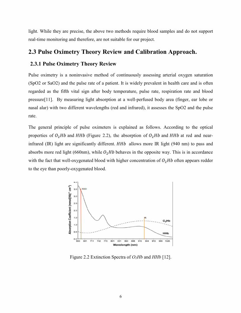
The respiration rate monitoring system consists a respiratory sensor belt, a micro-controller and a

wireless communication unit. The wearable system keeps measuring the patients’ respiratory

rates and sends them to a computer (Figure 3.2[22]).

Figure 3.2 Real-Time Respiration Rate Monitor System Diagram.

13

3.2.3 Respiratory Sensor Belt Development

The sensor belt is designed to acquire the raw signal of breathing events from the COPD

patients. In our design, a conductive rubber cord is selected for the sensor belt due to its

functionality and low cost (Figure 3.3). The cord is made of carbon-black impregnated rubber

and has an electrical resistance that increases gradually when stretched. With the conductive

rubber cord strapped around the chest, the thoracic or abdominal contraction and expansion

during breathing could be converted to electrical signals. The rubber cord is fixed on an elastic

band and used as a sensor belt for the respiratory measurement (Figure 3.4).

Figure 3.3 Conductive Rubber Cord.

Figure 3.4 Conductive Rubber Cord Fixed on an Elastic Band.

3.2.4 Microcontroller and Hardware Design

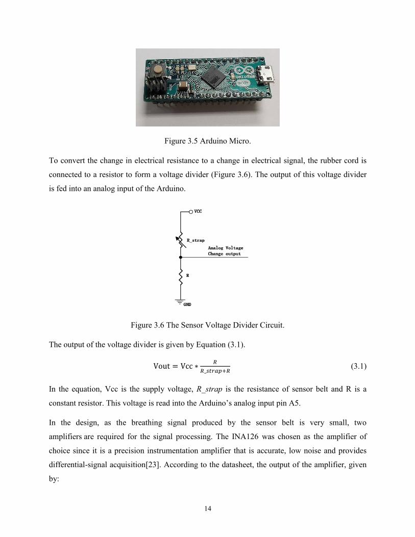
Due to its simplicity, small size and its relatively good computing power, Arduino Micro is

selected as the microcontroller board for the project. It is the smallest board of the Arduino

family and is suitable for the portability demand of the project (Figure 3.5).

14

Figure 3.5 Arduino Micro.

To convert the change in electrical resistance to a change in electrical signal, the rubber cord is

connected to a resistor to form a voltage divider (Figure 3.6). The output of this voltage divider

is fed into an analog input of the Arduino.

Figure 3.6 The Sensor Voltage Divider Circuit.

The output of the voltage divider is given by Equation (3.1).

Vout = Vcc ∗𝑅

𝑅_𝑠𝑡𝑟𝑎𝑝+𝑅 (3.1)

In the equation, Vcc is the supply voltage, R_strap is the resistance of sensor belt and R is a

constant resistor. This voltage is read into the Arduino’s analog input pin A5.

In the design, as the breathing signal produced by the sensor belt is very small, two

amplifiers are required for the signal processing. The INA126 was chosen as the amplifier of

choice since it is a precision instrumentation amplifier that is accurate, low noise and provides

differential-signal acquisition[23]. According to the datasheet, the output of the amplifier, given

by:

15

VO = ( 𝑉𝑖𝑛+ − 𝑉𝑖𝑛−) G. (3.2)

Where, G = 5 + 80kΩ / 𝑅𝐺

The Vin+ pins of the amplifiers in Figure 3.7 are connected to the Arduino digital output pins to

give a reference value. As the input analog signal changes with the expansion/retraction of the

chest, the reference value is set as the average input to the 𝑉𝑖𝑛−, so that the breathing signal is

amplified properly and output of amplifier is zero when there is no breathing.

VCC

R_strap

R1 +

-INA126

C1

Ref1 in

put f

rom

Arduino Digital

pin D3

R2

GND

+

-INA126

C2

Ref2 input from

Arduino

Digital

pi

n D5

R3

GND

Output to Arduino analog pin A3

GND

12



Figure 3.7 Schematic of the Hardware Connection.

For the first amplifier, R2 and C1 constitute a first order passive low pass filter, where the cut-off

frequency (fc) is given by using the Equation (3.3).

fc= 1/(2𝜋𝐶 ∗R). (3.3)

This circuit filters the high frequency noise from the output of the Arduino’s digital output pin

and feeds the resulting signal into the input of the INA126. Similarly, R3 and C2 fulfill the same

function for the second amplifier. The outputs of the two amplifiers are connected to the

Arduino’s analog input pins A1 and A3 for breathing rate calculation. Figure 3.7 shows the

general schematic diagram of the hardware connection. Figure 3.8 is the PCB (print circuit board)

of the hardware. The Arduino micro is connected to the testing board during the testing.

16

Figure 3.8 PCB of the Designed Circuit.

A pair of XBee wireless communication modules (part number XB24-Z7WIT-004) from Digi

International were selected in the project to provide wireless connectivity between the Arduino

board and the computer. The modules use the IEEE 802.15.4 networking protocol for fast point-

to-multipoint networking with low power consumption. In the wireless respiration rate monitor

system, the transmitter module is connected to the PCB of the testing board and the receiver

module is connected to a computer via an adapter board.

Figure 3.9 XBee Wireless Module.

3.2.5 Software Design

The software of the system is programmed in C with the Arduino Software (IDE). The running

process of the program is shown below.

https://www.digikey.ca/en/supplier-centers/d/digi-international

https://www.digikey.ca/en/supplier-centers/d/digi-international

17

Figure 3.10 Program Flow Chart.

After the initialization of variables, the program executes the setup(). In this part, it keeps

reading the analog signal of the pin A5 and A1 for 6 seconds each to get the average breathing

signal values from the sensor belt. Then, these values are written to Vin+ of the corresponding

amplifiers as reference values. Afterwards, the program waits for the first breathing and

memorizes the first breathing event system time T1 using the millis() function. The program

18

waits for the sensor belt signal to go low for a certain time T before detecting the next breathing

signal T2. This adjustable time T helps reduce false detections by setting the minimum time

interval between two valid consecutive respiration events. When the second breathing event

occurs, system time T2 is measured and the program calculates the elapsed time T2 – T1. Thus,

the elapsed time is the time interval between the two consecutive respirations. Finally, the real-

time respiratory rate R (breaths per minute) could be calculated with Equation (3.4).

R =6000/ (T2 – T1). (3.4)

After calculation, the R value is wirelessly transferred to a computer through the serial

communication port. The program runs in a loop and keeps detecting the breathing event and

sending the data during the testing.

As noises are usually introduced by the sensor belt and the hardware itself, we used an existing

library to smooth out the analog output signals by averaging consecutive output readings.

3.3 Initial Design of the Pulse Oximeter

In this section, the design process of the pulse oximeter is presented. Before introducing the

implementation details, a functional block diagram of the design is presented (Figure 3.11).

The optical system in the diagram emits red and IR lights alternatively under the control of the

LED drive circuit and microcontroller. Thus, a plethysmography (PPG) signal of the test subject

is produced on the side of PD. The signal is then amplified and filtered before being sent to the

10-bit ADC module of the microcontroller. At the microcontroller side, the analog PPG signal (0

to 5volts) is converted to digital numbers (0 to 1023) with the built-in ADC. With the proper

algorithm, the R value in Equation (2.4) and the heart rate are calculated. The desired data from

the microcontroller is transferred to the computer using the wireless module via its universal

asynchronous receiver/transmitter port (UART). The detailed process is presented in the

following sections.

19

Figure 3.11 Pulse Oximeter Design

3.3.1 Hardware Design and Components Selection

3.3.1.1 Microcontroller Selection

The microcontroller is at the heart of the system. It controls the entire system and deals with the

signals coming from the sensors. Considering the hardware requirements, the Arduino UNO

board was chosen for this application (Figure 3.12). The board is designed with an Atmel328P

processor and combines many features such as a 10-bit ADC, internal and external interrupts, 14

digital I/O pins and 6 analog input pins, which are all necessary for the design.

20

Figure 3.12 Arduino UNO

3.3.1.2 Optical Probe Selection

As mentioned above, LEDs and PD are required to send and receive optical signals. Depending

on the relative position of LEDs and PD, there are two methods of sending the light to the

measuring tissues: transmissive method and reflective method.

The transmissive method is a traditional method applied in most of the commercial pulse

oximeters. For this method, the LEDs and PD are placed right opposite to each other with the

measuring site between them. The red or IR light emitted from the LEDs will travel through the

measured sites. Then, the residual light will reach the PD after the absorption. The typical

measuring sites for the transmittance probe are finger, ear lobe, nasal alar, toe for adults or the

foot or palm for infant. The reason for targeting these body tissues is that there is a much higher

vascular density than other body areas[24]. A clip-like probe is often used for this method to

hold the measured tissues.

The reflective method was first introduced by Brinkman and Zijlstra in 1949[25]. For this

method, the LEDs and PD are placed on the same side of the measuring site with the PD

receiving the reflected light signal from different depths underneath the skin. This method is

becoming more and more popular in recent years due to its flexibility of measuring sites. A

variety of body sites can be measured such as forehead, wrist, ankle, ear, etc.

Since tissue is highly forward scattering, the relative number of photons detected in reflective

mode is low. This will cause a relatively poor PPG signal. Therefore, for this method, sensors

should be well designed for better acquisition of the radial reflectance profile[26].

21

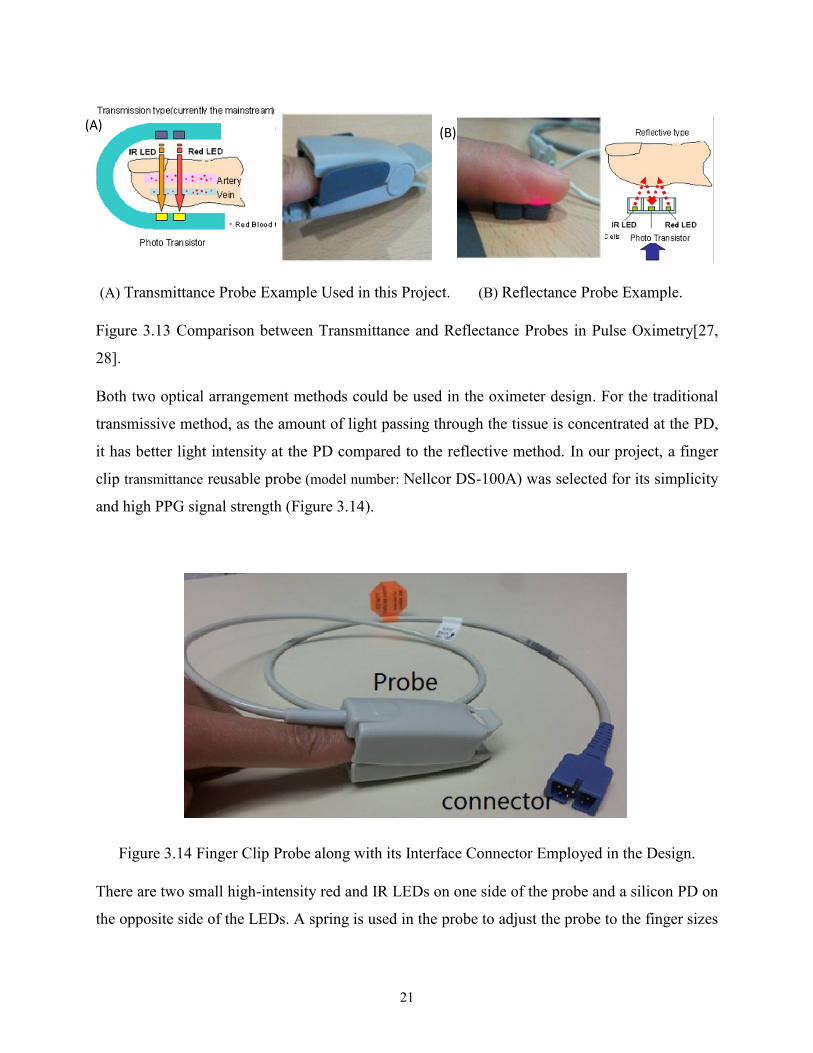
(A) Transmittance Probe Example Used in this Project. (B) Reflectance Probe Example.

Figure 3.13 Comparison between Transmittance and Reflectance Probes in Pulse Oximetry[27,

28].

Both two optical arrangement methods could be used in the oximeter design. For the traditional

transmissive method, as the amount of light passing through the tissue is concentrated at the PD,

it has better light intensity at the PD compared to the reflective method. In our project, a finger

clip transmittance reusable probe (model number: Nellcor DS-100A) was selected for its simplicity

and high PPG signal strength (Figure 3.14).

Figure 3.14 Finger Clip Probe along with its Interface Connector Employed in the Design.

There are two small high-intensity red and IR LEDs on one side of the probe and a silicon PD on

the opposite side of the LEDs. A spring is used in the probe to adjust the probe to the finger sizes

(A) (B)

22

of testing subjects. The probe is connected to the outer circuit through a 7-pin sub-D connector

(DB9). The schematic of the probe is shown in Figure 3.15.

Figure 3.15 Schematic of Finger Probe.

3.3.1.3 LED Drive Circuit

In the optical system of pulse oximeter, the red and IR LEDs are switched to emit light passing

through the testing finger. For different testing subjects, the residual light intensity at the PD may

differ from each other. This may be caused by the difference of finger thickness, arterial blood

volume and skin absorption. Thus, the light intensity needs to be adjusted for different

participants. For the optical system, we need to control both the illumination time and the

intensity of the red and IR light through the microcontroller. Figure 3.16 shows the schematic of

designed LED drive circuit. As shown in the probe schematic, the two LEDs are connected back

to back and only the red or the IR light can be turned on at a time. Based on the LED

configuration, an analog switch was used to control the LED in the design. For the light

intensity, it was adjusted by controlling the current through the LEDs. A digital to analog

converter (DAC) was used in the circuit to implement the current control.

23

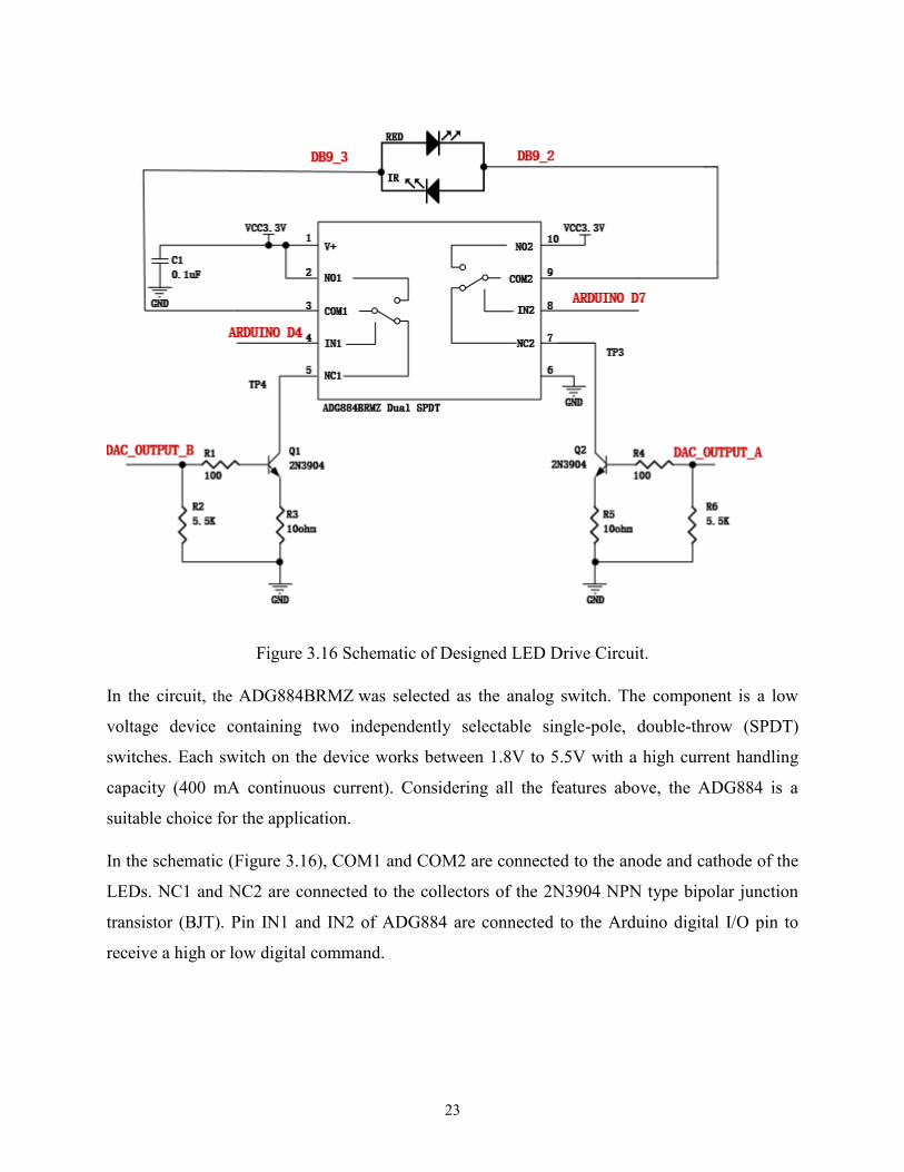
Figure 3.16 Schematic of Designed LED Drive Circuit.

In the circuit, the ADG884BRMZ was selected as the analog switch. The component is a low

voltage device containing two independently selectable single-pole, double-throw (SPDT)

switches. Each switch on the device works between 1.8V to 5.5V with a high current handling

capacity (400 mA continuous current). Considering all the features above, the ADG884 is a

suitable choice for the application.

In the schematic (Figure 3.16), COM1 and COM2 are connected to the anode and cathode of the

LEDs. NC1 and NC2 are connected to the collectors of the 2N3904 NPN type bipolar junction

transistor (BJT). Pin IN1 and IN2 of ADG884 are connected to the Arduino digital I/O pin to

receive a high or low digital command.

24

Table 3.1 shows the functionality of ADG884 with two kinds of input logic signals. According to

the table, when Arduino digital output D4(IN1) is 1 and D7(IN2) is 0, NC1 and NO2 are off and

NC2 and NO1 are on.

Table 3.1 Functionality of the ADG884 Input Logic Signal.

Functionality of the ADG884

Input Logic Signal NC1 and NO2 NC2 and NO1 LED statuts

IN1=0& IN2=1 ON OFF Red off & IR on

IN1=1& IN2=0 OFF ON Red on & IR off

In other words, the red LED anode is connected to the 3.3V Vcc and cathode is connected to the

collector of Q2. The equivalent circuit diagram is shown in Figure 3.17.

Figure 3.17 Red LED Current Control Circuit.

Similarly, when the Arduino digital output D4 (IN1) is 0 and D7 (IN2) is 1, the equivalent circuit

for the IR light becomes that of Figure 3.18.

Q2

25

Figure 3.18 IR LED Current Control Circuit.

Therefore, the switch of two LEDs is controlled by the digital signal from the Arduino digital I/O

pins.

For a LED, the current flowing from the anode to the cathode is defined as forward current with

the typical values ranging from 2 to 50 mA. The forward current determines the light intensity of

the LED. Hence, we can control the light intensity of the LEDs via the forward current. The

potential drop across the p-n junction of the diode (forward voltage) is often between 0.9 and 2.5

V.

Considering the circuit in Figure 3.9, the transistor Q1 acts as a controlled current sink, where

the current flowing in the base is determined by the base voltage of Q1, the resistor R1 and R3.

For the transistor with a gain of β, the forward current IC is β times of the base current IB. When

the transistor is turned on, there is a voltage drop across the base emitter junction which is about

0.7V.

If the DAC output is VDAC and the base voltage of the transistor is VB, the current flow the base

of transistor IB and the emitter current IE is expressed as follow.

IB = (VDAC - VB)/R1 (3.5)

IE = (VB-0.7)/R3 (3.6)

Q1

26

Since IC= β* IB and IE= IB+ IC, after derivation with Equation (3.5) and (3.6), we have the

LED forward current in Equation (3.7).

IC = β*(VDAC-0.7) / (R1+R3*(β+1)). (3.7)

Since VDAC is tightly controlled by the microcontroller, the gain of the transistor β can be

considered constant and R1 and R3 are fixed values, the forward current IC is essentially

determined by the microcontroller. In the circuit, the anode of the LED is connected to the 3.3V

power supply to provide enough forward voltage drop.

For the DAC, the MCP4728 from Microchip Technology was selected in the design. The device

is a 12-bit DAC with nonvolatile memory (EEPROM) and four output channels. It uses a two-

wire I2C (Inter-Integrated Circuit) serial interface to communicate with the Arduino and works

as a slave device when connected to the I2C bus line. The configuration such as input codes,

device configuration bits, and address bits are programmable to its nonvolatile memory by using

I2C serial interface commands. The nonvolatile memory makes it possible to hold the DAC

settings during power-off time, allowing the outputs to be available immediately after power-up.

In the design, a 0.1µF bypass capacitor together with an additional 10 µF capacitor in parallel

was connected to the power supply to attenuate the high-frequency noise from the application

board. The 5.1kΩ pull-up resistors for SCL and SDA are suitable for Standard (100 kHz) and

Fast (400 kHz) modes (Figure 3.19).

27

GND

GND

GND

R8

5.1KR7

C3 0.1uF

C2 10uF

GND

VCC3.3V

1

2

3

4

5

DAC

VDD

SCL

SDA

nlDAC

RDY/nBSY VOUTA

VOUTB

VOUTC

VOUTD

VSS 10

9

8

7

6

MCP47281nF 1nF

ARDUINO A3 for I2C

ARDUINO A4 for I2C

C4

DAC_OUTPUT_B

DAC_OUTPUT_A

5.1K

Figure 3.19 DAC Schematic.

Two output channels of the device are connected to the base terminals of Q1 and Q2. A 1 𝑛𝐹

capacitor is used to stabilize the output voltage. The channel output voltage is associated with its

configuration bit settings and DAC input code. It is calculated with the equation below.

Vout = VDD*Dn/4095. (3.8)

In this equation, Dn is the DAC input value (0 to 4095) that is set in the Arduino program and

VDD is the reference voltage. Therefore, the red and IR light forward currents are controlled by

the Arduino microcontroller.

3.3.1.4 Signal Conditioning

The PD in the probe generates a current when receiving the light that travels through the finger.

Since the light received by the PD also includes ambient light, the current generated by the PD

will also be mixed with noise. This current is a small signal and that is generally a few hundreds

of nanoamps according to our tests. To get a clean and proper PPG signal in order to determine

the oxygen saturation and heart rate, the raw signal needs to be amplified and filtered before

being sent to the Arduino.

The PD current needs to be converted to voltage before it is filtered. A transimpedance amplifier

(TIA) is used for this purpose. The precision operational amplifier LT1677 from Linear

Technology was selected in the project for its rail-to-rail input and output, low input bias current

and low noise features. Figure 3.20 presents the implemented circuit with LT1677.

28

R11

3.3V

+

-

PD

GND

1.2K 10KR9 R10

4. 7M

C6270PF

Transimpedance AmplifierLow Pass (LP)cut offfc = 125 HZ, Gain = 4.7M

3.3V

TIA

Figure 3.20 Current to Voltage Converter in the Circuit.

In the circuit, the input resistance of the amplifier is so high that all the current from the PD must

go through the feedback resistor R11. The gain of the TIA is therefore determined by R11. If the

current from the PD cathode is I, the output voltage will be given by Equation (3.9). Since the

current is very small, a 4.7 Mohm resistor was selected for the required gain.

Vout = I*R11. (3.9)

A capacitor C6 is placed in parallel with the transimpedance resistor R11. The TIA, R11 and C6

together constitute a first order active low pass filter, where the cut-off frequency (fc) is given by

using the Equation (3.10).

fc= 1/(2𝜋𝐶 ∗R). (3.10)

As this is the first stage of the low pass filter, only the high frequency noises will be removed.

Thus, a 125Hz cut-off frequency was chosen and this was accomplished using a 270 pF capacitor

after calculation with Equation (3.10). The Bode plot of the filter is presented in Figure 3.21.

29

Figure 3.21 Bode Plot of the First Active Filter[29].

At low frequencies, the input signal is passed directly to the output with a gain of the TIA until it

reaches the cut-off frequency fc at which point the gain is 1/√2 (-3dB) of the maximum gain.

After this point, the response of the circuit is attenuated with slope of -20dB/Decade.

The non-inverting input of the LT1677 is connected to a voltage from the voltage divider.

Therefore, the initial amplitude level of the TIA output is shifted. This step converts the positive

and negative output signal of TIA into a positive-only range signal for further conditioning.

Finally, the signal is shifted to a range between 0 and 5V when sent to the Arduino ADC. With

Equation (3.11), it is possible to calculate the output of the voltage divider network. The level

shift voltage is set to 0.35V:

Vout = R9*VCC/(R9+R10). (3.11)

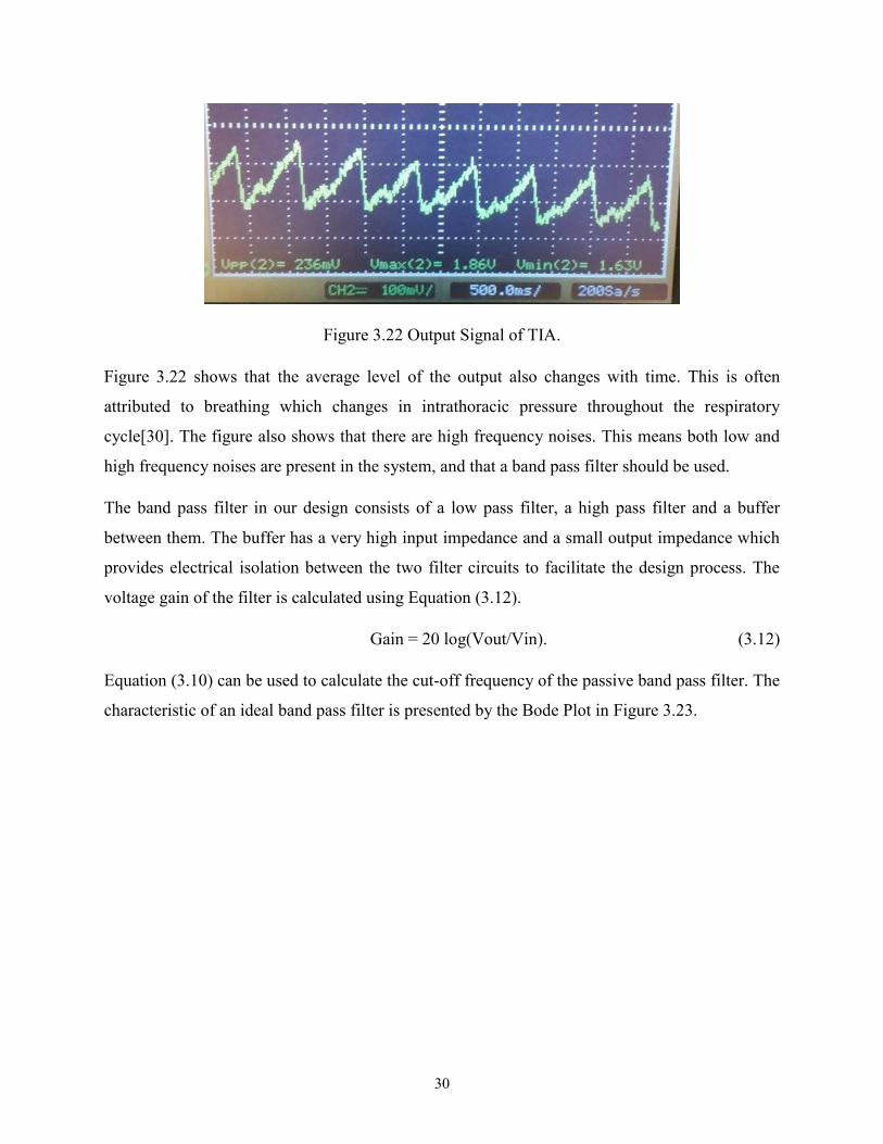
Figure 3.22 shows the output the of the TIA with the previously described configuration.

30

Figure 3.22 Output Signal of TIA.

Figure 3.22 shows that the average level of the output also changes with time. This is often

attributed to breathing which changes in intrathoracic pressure throughout the respiratory

cycle[30]. The figure also shows that there are high frequency noises. This means both low and

high frequency noises are present in the system, and that a band pass filter should be used.

The band pass filter in our design consists of a low pass filter, a high pass filter and a buffer

between them. The buffer has a very high input impedance and a small output impedance which

provides electrical isolation between the two filter circuits to facilitate the design process. The

voltage gain of the filter is calculated using Equation (3.12).

Gain = 20 log(Vout/Vin). (3.12)

Equation (3.10) can be used to calculate the cut-off frequency of the passive band pass filter. The

characteristic of an ideal band pass filter is presented by the Bode Plot in Figure 3.23.

31

Figure 3.23 Bode Plot of an Ideal Passive Band Pass Filter[31].

As shown in Figure 3.23, at low frequencies, the gain of the filter changes with a slope of

+20dB/Decade until the frequency reaches the cut-off frequency of the low pass filter ƒL. The

gain continues to be at its maximum value until it reaches the cut-off frequency of the high pass

filter ƒH, then it is attenuated with a slope of -20dB/Decade.

To calculate the cut-off frequency of the band pass filter, the characteristics of the signal of

interest (the heart rate) are analyzed. A normal resting heart rate for adults ranges from 60 to 100

beats per minute (BPM) whereas a well-trained athlete might have a resting heart rate closer to

40 BPM[32]. In the current project, heart rates between 40 and 180 BPM (0.7 Hz and 3Hz) will

be considered. Therefore, the pass band of the filter will be between 0.7 Hz and 3Hz. The cut-off

frequency of each stage of the passive band pass filter was calculated using Equation (3.10). The

designed band pass filter is shown in Figure 3.24.

32

Figure 3.24 Schematic of the Designed Band Pass Filter.

Figure 3.25 shows the frequency response curve of the designed band pass filter.

Figure 3.25 Bode Plot of the Designed Band Pass Filter.

An output example signal from oscilloscope is shown in Figure 3.26.

33

Figure 3.26 Signal at the Output of Band Pass Filter.

As the figure shows, the low frequency noise was attenuated compared to Figure 3.22 and there

were still some high frequency noises in the system. Since the band pass filter is a passive filter

the gain of signal is also smaller compared to the output of the TIA.

In the filter (Figure 3.24), the output of the buffer is connected to the Arduino ADC to read the

DC level which is an important parameter in the oxygen saturation calculation. The reason for

reading the DC value at this point is that the DC signal is removed after the high pass filter.

Since the passive band pass filter can’t remove all the noise, a first order active low-pass filter

was introduced (Figure 3.27). LT1677 operational amplifier was also used in this filter design.

34

Figure 3.27 Active Low Pass Filter.

The gain can be calculated as follows:

𝑉𝑖𝑛−0

𝑅15 =

0−𝑉𝑜𝑢𝑡

1

1𝑅14+𝑗𝜔𝑐9

(3.13)

After derivation, we have equation below.

𝑉𝑜𝑢𝑡

𝑉𝑖𝑛=

𝐻0𝜔0

𝑆+𝜔0 with |

𝑉𝑜𝑢𝑡

𝑉𝑖𝑛|=|𝐻0|

𝜔0

√𝜔02+𝜔2

(3.14)

In this equation, 𝐻0 is -R14/R15 and 𝜔0 is 1/(R14*C9). For this low pass filter, the cutoff

frequency is calculated with Equation (3.10) where R14 is used for calculation. At high

frequencies (ω>>𝜔0) the capacitor acts as a short circuit and the gain of the amplifier drops to

zero. At very low frequencies ( ω<< 𝜔0) the capacitor is an open and the gain of the circuit is

Ho.

It is important to note that the DC voltage of Vcc/2 (Vcc is 3.3V) is supplied to R13 and the non-

inverting input of the op-amp (Figure 3.24 & Figure 3.27). The purpose of this input voltage is to

superimpose the AC signal to a DC level equal to Vcc/2. As stated in the previous section, to

35

interface with the Arduino ADC, the amplitude range of the AC voltage should be 0 to 3.3V. To

generate this voltage, a voltage divider circuit with a LT1677 amplifier (Figure 3.28) was

introduced. The operational amplifier buffer in the circuit was also used to eliminate the

interaction with the adjacent circuit.

Figure 3.28 Voltage Divider Circuit

With all the described signal conditioning, the resulting signal was suitable for interfacing with

the Arduino ADC (Figure 3.29).

Figure 3.29 Output of the Last Filter as a Response to the IR LED.

36

During the hardware testing, the circuit is implemented on a breadboard since it was simpler to

make adjustments as required. Integrating the components and the microcontroller onto a PCB

would make the device more portable and easier to use in the further research.

3.3.2 Algorithm and Software Implementation.

After the signal conditioning, the amplified red and IR PPG signals were ready for analysis. This

section presents how the analog signal was processed in the Arduino program to calculate the

SpO2 and heart rate.

3.3.2.1 Signal Feature Analysis

Before explaining the detailed algorithm, an analysis of the filtered signal is presented.

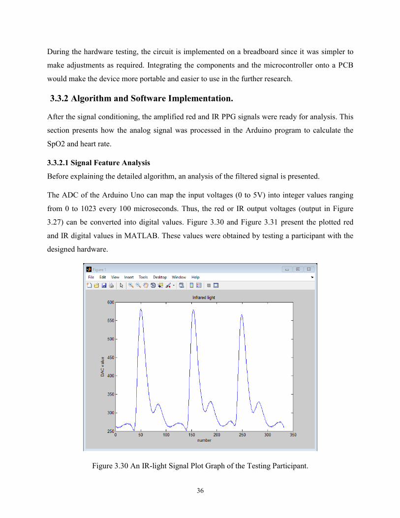
The ADC of the Arduino Uno can map the input voltages (0 to 5V) into integer values ranging

from 0 to 1023 every 100 microseconds. Thus, the red or IR output voltages (output in Figure

3.27) can be converted into digital values. Figure 3.30 and Figure 3.31 present the plotted red

and IR digital values in MATLAB. These values were obtained by testing a participant with the

designed hardware.

Figure 3.30 An IR-light Signal Plot Graph of the Testing Participant.

37

Figure 3.31 A Red-Light Signal Plot Graph of the Testing Participant.

In the two above figures, the x-axis and the y-axis are unitless. The y axis is the digitized voltage

with a range of 0 to 1023. The x-axis is the sample number. The sample frequency of the

Arduino ADC is 100KHz.

As the IR light penetrates the body deeper than red light, it generates a larger peak to peak value.

It is interesting to note that, when the signal goes down to the base level, there is a small dip

(also called dicrotic notch)[33]. It is caused by the closure of the aortic valve and it needs to be

considered in the algorithm to avoid calculation errors.

The time interval between the two consecutive heartbeats is also known as the inter beat interval

(IBI). A sample IBI is shown in Figure 3.31 and it will be explained in detail in the following

chapter. The trough and peak values correspond to the points where the wave presents the

smallest and largest ADC values, respectively. The Thresh level, as indicated in the figure,

corresponds to half of the sum of peak and trough values.

38

3.3.2.2 Software Design

The heart rate can be calculated with the IBI. To perform this task, the moment at which a

heartbeat occurs can be determined using several methods. Some researchers consider the point

at which the signal reaches 25% or 50% of maximum height of the PPG signal[34]. In this

project, the IBI is obtained by measuring the time interval between two adjacent wave points

where the fast-rising wave reaches 50% of its maximum value. Consider Figure 3.31, for

example. The time interval between A and B is a sample IBI.

To calculate SpO2, as stated in Section 2.3, it is calculated using Equation (2.5). To obtain the R

value in this equation, the red and IR LEDs are switched on and off to measure their relative AC

and DC values (see Equation (2.4)). The AC value of the red or IR signal is the peak to trough

value (see Figure 3.31). The DC value is the average value of the signal.

To measure the IBI, the Arduino needs to have a regular sampling rate. For that purpose, the

program uses a timer module and sets an interrupt every 2ms (500 Hz sampling rate). When the

interrupt is triggered, the program will pause its current activity and execute the interrupt service

routine (ISR).

When the program begins, it sets up different variables including the DAC output parameters.

Afterwards, the red LED is switched on and finally, the timer interrupt is started.

The IBI, AC and DC values are the key factors used to calculate the heart rate and SpO2. The

pseudo-code of Algorithm 1 in Figure 3.32 explains how these values are determined during a

pulse signal.

39

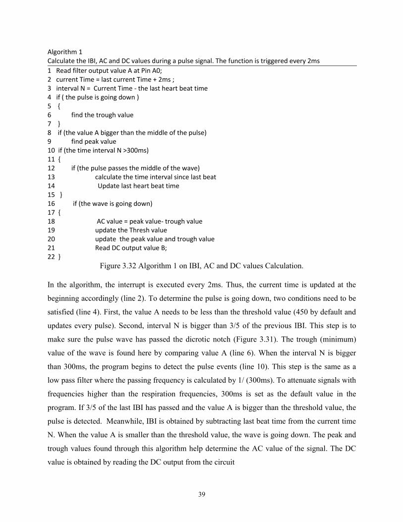
Algorithm 1 Calculate the IBI, AC and DC values during a pulse signal. The function is triggered every 2ms

1 Read filter output value A at Pin A0; 2 current Time = last current Time + 2ms ; 3 interval N = Current Time - the last heart beat time 4 if ( the pulse is going down ) 5 6 find the trough value 7 8 if (the value A bigger than the middle of the pulse) 9 find peak value 10 if (the time interval N >300ms) 11 12 if (the pulse passes the middle of the wave) 13 calculate the time interval since last beat 14 Update last heart beat time 15 16 if (the wave is going down) 17 18 AC value = peak value- trough value 19 update the Thresh value 20 update the peak value and trough value 21 Read DC output value B; 22

Figure 3.32 Algorithm 1 on IBI, AC and DC values Calculation.

In the algorithm, the interrupt is executed every 2ms. Thus, the current time is updated at the

beginning accordingly (line 2). To determine the pulse is going down, two conditions need to be

satisfied (line 4). First, the value A needs to be less than the threshold value (450 by default and

updates every pulse). Second, interval N is bigger than 3/5 of the previous IBI. This step is to

make sure the pulse wave has passed the dicrotic notch (Figure 3.31). The trough (minimum)

value of the wave is found here by comparing value A (line 6). When the interval N is bigger

than 300ms, the program begins to detect the pulse events (line 10). This step is the same as a

low pass filter where the passing frequency is calculated by 1/ (300ms). To attenuate signals with

frequencies higher than the respiration frequencies, 300ms is set as the default value in the

program. If 3/5 of the last IBI has passed and the value A is bigger than the threshold value, the

pulse is detected. Meanwhile, IBI is obtained by subtracting last beat time from the current time

N. When the value A is smaller than the threshold value, the wave is going down. The peak and

trough values found through this algorithm help determine the AC value of the signal. The DC

value is obtained by reading the DC output from the circuit

40

With the algorithm above, the IBI time, the AC and DC values can be calculated for a single

beat. Instantaneous values, however, are prone to noise. In addition, the IBI tends to vary from

one heartbeat to the next and therefore, an average value would be more interesting for our

application. Therefore, we implemented a moving average filter as shown in Figure 3.33.

Algorithm 2 buffer shifting algorithm to get an averaged IBI and calculate BPM 1 IBI = Sample Time – last heart beat Time; 2 if (the first beat is true) 3 wait second beat 4 5 if (the second beat is true) 6 for item 0 to 9 7 set IBI_ARRAY [item] = IBI 8 end for 9 10 else 11 for index 0 to 8 12 shift the array item as Figure 3.23 indicates 13 calculate the sum of IBI_ARRAY 14 end for 15 IBI_ARRAY [9] = new tested IBI 16 sum IBI = sum IBI + IBI_ARRAY [9]

17 Average of the array ：AVERAGE is SUM_IBI / 10 18 Heart rate BPM is 60000 / AVERAGE 19

Figure 3.33 Algorithm 2 on Heart Rate Calculation.

In Figure 3.33, since the IBI is calculated by subtracting the previous beat time, the IBI from the

first beat is discarded. The array of IBI is initialized by giving the new IBI value to each of its

item at the second beat (line 6 and 7). Beginning from the third one, the IBI values are processed

by the moving average method. The heart rate is calculated from the average of the IBI.

As the program runs, the new IBI value are placed in the position 9 of the array with the older

values being shifted to the right. The value at position 0 is discarded when new data arrive.

Figure 3.34 illustrates this algorithm. The output of the heart rate is determined by the average of

last nine pulse waves. Through experiments, it was found that 9 heart beats were the minimum

value that would provide good results.

41

IBI(9) IBI(8) IBI(7) ... IBI(2) IBI(1)

IBI(9) IBI(8) IBI(7) ... IBI(2) IBI(1)

NEW IBI

Discarded

Current pulse

Next pulse

Figure 3.34 Buffer Shifting for IBI Values.

The flowchart in Figure 3.35 describes the program. To calculate the SpO2, one of the LEDs

remains ON for 8 heart beats while the other LED is OFF. The roles are then inversed for the

following 8 heart beats. The values from the 16 heart beats are then used to calculate SpO2.

For most of pulse oximeters on the market, the LED is switched rapidly between red and IR

(about several milliseconds). In the prototype, the LED is switched every 8 heart beats. The

benefit of this new approach is that it reduces the influence of light switching noise. Meanwhile,

as the value of SpO2 is calculated every 8 heart beats, the result is already an averaged

representative value.

42

Figure 3.35 Flow Chart of the Program.

43

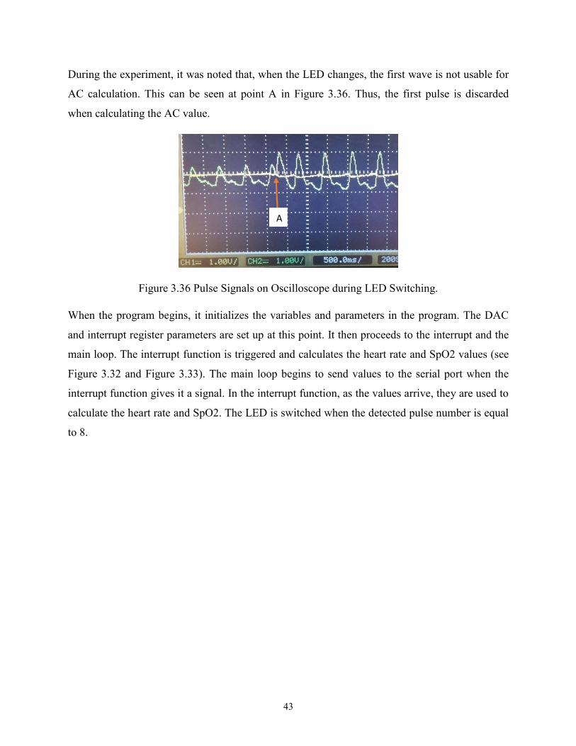
During the experiment, it was noted that, when the LED changes, the first wave is not usable for

AC calculation. This can be seen at point A in Figure 3.36. Thus, the first pulse is discarded

when calculating the AC value.

Figure 3.36 Pulse Signals on Oscilloscope during LED Switching.

When the program begins, it initializes the variables and parameters in the program. The DAC

and interrupt register parameters are set up at this point. It then proceeds to the interrupt and the

main loop. The interrupt function is triggered and calculates the heart rate and SpO2 values (see

Figure 3.32 and Figure 3.33). The main loop begins to send values to the serial port when the

interrupt function gives it a signal. In the interrupt function, as the values arrive, they are used to

calculate the heart rate and SpO2. The LED is switched when the detected pulse number is equal

to 8.

A

44

4. Experiments and Results

After the instruments were designed, a series of experiments were carried out to evaluate the

performance of the designed prototypes. For the respiration rate monitoring system, the

measurements were compared to visual observations. For the pulse oximeter prototype, the

measurements were compared to the results of a reference commercial pulse oximeter under the

same testing conditions. In this section, we present the test methods and the results obtained.

4.1 Respiration Rate Monitor System Test.

4.1.1 Material and Method

After respiration rate monitor system was designed, a series of experiments were carried out to

test of the designed prototype.

Two healthy (one female and one male), non-smoking students aged 25 and 32 participated the

evaluation. In order to participate in the study, the students had to be free from respiratory

diseases, obesity, cardiovascular problems. The ambient air temperature in the laboratory is

about 23°C during the whole test.

Figure 4.1 The Designed Respiration Monitor System during the Test.

Two measurements were performed under different conditions for the analysis. The first

measurement evaluated the participants at rest and the latter one was performed when the

participants had a higher breathing rate. Since breathing rate could be self-controlled, the

participants were instructed to breathe rapidly to get a higher breathing rate. An oscilloscope was

used to monitor the analog signals sent to the Arduino during the test. The real-time breathing

time and breathing rate were sent to a computer via XBee wireless transmission modules.

45

4.1.2 Testing Results

During the test, the respiration rate monitor system presented high accuracy and every respiration

event was detected by the instrument. For each respiration event, the time interval between the

two consecutive respirations (elapsed time) and the real-time respiratory rate were sent to a

computer through wireless transmission.

Figure 4.2 and Figure 4.3 present the elapsed time (in milliseconds) and the corresponding real-

time respiration rate (breaths per minute) received from Arduino at the two different respiration

events of a participant.

Figure 4.2 Elapsed time (milliseconds) and the Corresponding Real-time Respiration Rate

(breaths per minute) Received from Arduino At Rest State.

46

Figure 4.3 Elapsed Time (milliseconds) and the Corresponding Real-time Respiration Rate

(breaths per minute) Received from Arduino at A Rapid Respiration Rate.

During the test, the respiratory events of the participants were monitored visually and showed

high accordance with the prototype measuring results. Meanwhile, on the oscilloscope, the

waveform of each respiration was monitored during the test. Figure 4.4 presents oscilloscope

waveform corresponding to the last four respiratory events of Figure 4.3. We can find the

estimated elapsed times from the waveform are consistent with the received data in Figure 4.3.

Figure 4.4 Signal Waveforms on Oscilloscope in the Rapid Respiration Test.

47

According to the testing results, the respiration rate monitor system presented high accuracy in

real-time respiration detection and is ready to be used for training COPD patients in remote

locations.

4.2 Pulse Oximeter Test

4.2.1 Material and Method

A group of five healthy, non-smoking students (2 females and 3 males) participated in the

validation of the prototype. They ranged in age between 22 and 32 years (25.6 ±3.7 years). In

order to participate in the study, the students had to be free from respiratory diseases, obesity,

cardiovascular problems or severe contact allergies to latex or other materials in pulse oximetry

sensors. The ambient air temperature in the laboratory is about 23°C during the whole test.

To provide reference to validate the prototype, an oximeter is needed for the tests. As introduced

in Section 2.2, the arterial blood gas analyzers and CO-oximetry are precise to measure the

oxygen saturation. Since they require blood samples and do not support real-time monitoring,

they are not suitable to provide reference. A commercial pulse oximeter from Choice

Technology (MD300c) was used to provide real-time reference in the tests. An oscilloscope was

used to monitor the analog input signals to the Arduino at the same time.

At the beginning of the tests, the DAC output parameters were adjusted for each participant to

obtain a proper signal level. During the test, the probe of the prototype was attached to the

middle finger. The reference oximeter was attached to the index finger for comparison (Figure

4.5). For each participant, the test results were measured continuously over a time-span of 3

minutes. The heart rate and calculated R values from the designed prototype were printed to the

screen while the values of the MD300c were recorded at the same time (Figure 4.5). For the

MD300c, since it had no digital or analog output for the results, readings were recorded by hand

throughout the test.

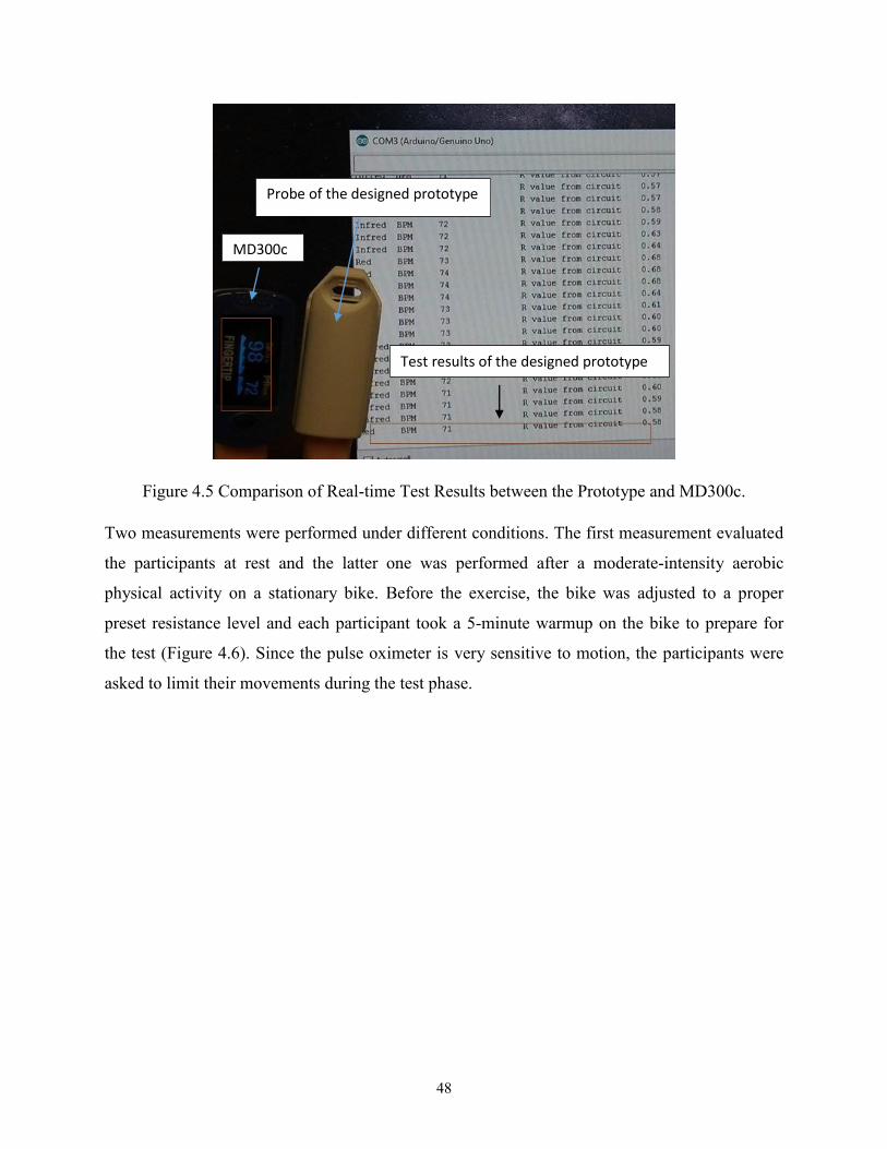
48

Figure 4.5 Comparison of Real-time Test Results between the Prototype and MD300c.

Two measurements were performed under different conditions. The first measurement evaluated

the participants at rest and the latter one was performed after a moderate-intensity aerobic

physical activity on a stationary bike. Before the exercise, the bike was adjusted to a proper

preset resistance level and each participant took a 5-minute warmup on the bike to prepare for

the test (Figure 4.6). Since the pulse oximeter is very sensitive to motion, the participants were

asked to limit their movements during the test phase.

MD300c

Probe of the designed prototype

Test results of the designed prototype

49

Figure 4.6 Stationary Bike Used in the Test.

Average heart rate and SpO2 measured using the MD300c and the prototype were calculated

after the experiment. The percentage error was also selected for the result analysis using

Equation (4.1).

Percentage Error = | Reference value − Prototype value

Reference value | ∗ 100 (4.1)

Simple linear regression method was used for modeling the results relationship between the

MD300c and the prototype.

4.2.2 Testing Results

The average results and the percentage of error for heart rate and SpO2 of all participants are

listed in Table 4.1.

50

Table 4.1 Average Results and Percentage of Error for Heart Rate and SpO2.

Reference Pulse Oximeter Prototype Pulse Oximeter Percentage Error

SpO2 (%) Heart Rate SpO2 (%) Heart Rate SpO2 Heart Rate

98.25 96.93 96.30 97.41 1.96 0.50

For the heart rate tests, the test results of the prototype showed high consistency and accuracy

compared to the outputs of the reference MD300c during the entire test.

The calculated heart rate percentage error between the prototype and the MD300c was 0.5%

(Table 4.1) which means that the designed prototype showed high accuracy in the heart rate tests.

The test results were also analyzed by linear regression. Figures 4.7 and 4.8 show the comparison

of heart rate data measured by the prototype and the reference MD300C at rest and after

exercise. The solid line represents the linear regression line of the test results. The reference

dashed line represents the linear line on the assumption that the prototype and the reference

MD300C results are equal. The relative R2 are separately 0.95 and 0.93 under the two

conditions, indicating that the data measured by the prototype device correlates very well with

the reference device.

51

Figure 4.7 Comparison of Real-time Heart Rate at Rest.

Figure 4.8 Comparison of Real-Time Heart Rate after Prescribed Exercises.

y = 1.0679x - 3.915R² = 0.9533

y = xR² = 1

60

65

70

75

80

85

90

95

100

60 65 70 75 80 85 90 95 100

Pro

toty

pe

Dev

ice

Reference commercial pulse oximeter

Heart rate(Paticipants at rest)

prototype Device liner(prototype device) liner(1:1)

y = 1.079x - 8.7871R² = 0.9298

y = xR² = 1

80

85

90

95

100

105

110

115

120

125

130

80 85 90 95 100 105 110 115 120 125

Pro

toty

pe

Dev

ice

Reference commercial pulse oximeter

Heart rate(After exercising)


52

For the SpO2 tests, as stated in the literature review, Equation (2.5) is selected as a linear

approximation to the empirical calibration curve. The measured results were rounded to the

nearest decimal. This is conducive to analyzing the trends of SpO2 changes.

The calculated SpO2 percentage error between the prototype and the MD300c was 1.96% (Table

4.1). During the test phase, we found the SpO2 results of the reference MD300c stayed relatively

stable between 97% and 99%. At the same time, the results fluctuated between 93% and 99% for

our prototype.

Figure 4.9 shows the comparison of the oxygen saturation data. The solid line represents the

linear regression line. The reference dashed line represents the assumption that the prototype and

the reference MD300C results are equal. The R2 value is equal to 0.56, indicating that the data

measured by the prototype device does not correlate very well with the reference device. We

believe that this may due to the empirical calibration equation and the MD300c measurement

accuracy, as the measurement accuracy of MD300C is ±2% in the test measurement range.[35]

Figure 4.9 Comparison of SpO2 Measurement between the Prototype and MD300c.

y = 1.4884x - 50.168R² = 0.5565

y = xR² = 1

94

95

96

97

98

99

100

94 95 96 97 98 99 100

Pro

toty

pe

Pu

lse

Oxi

met

er D

ata

(%)

Reference commercial pulse oximeter data

SpO2


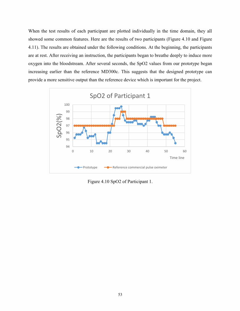
53

When the test results of each participant are plotted individually in the time domain, they all

showed some common features. Here are the results of two participants (Figure 4.10 and Figure

4.11). The results are obtained under the following conditions. At the beginning, the participants

are at rest. After receiving an instruction, the participants began to breathe deeply to induce more

oxygen into the bloodstream. After several seconds, the SpO2 values from our prototype began

increasing earlier than the reference MD300c. This suggests that the designed prototype can

provide a more sensitive output than the reference device which is important for the project.

Figure 4.10 SpO2 of Participant 1.

94

95

96

97

98

99

100

0 10 20 30 40 50 60

SpO

2(%

)

Time line

SpO2 of Participant 1

Prototype Reference commercial pulse oximeter

54

Figure 4.11 SpO2 of Participant 2.

94

95

96

97

98

99

100

0 10 20 30 40 50 60 70 80

SpO

2(%

)

Time Line

SpO2 of Participant 2

Prototype Reference commercial pulse oximeter

55

5. Conclusion and Future Work

The aim of this research was to design a low cost wireless system to measure three physiological

parameters: respiratory rate, oxygen saturation and heart rate for training COPD patients

remotely.

For the respiratory rate measurement, a respiratory sensor belt was designed to measure the

respiratory rate. A conductive rubber cord was selected to construct the sensor belt due to its

functionality and low cost. Filters and amplifiers were designed for signal conditioning and an

algorithm was designed on a microcontroller to measure the respiration rate. The final output

was sent to a computer using Xbee wireless modules. It was evaluated with experiments and

demonstrated high accuracy for respiratory detection.

For the oxygen saturation and heart rate monitoring, a pulse oximeter was designed and built to

measure these parameters at the fingertip. A group of volunteers participated in the test program

in the laboratory. A commercial pulse oximeter was used as a reference for performance

comparison. Two evaluation metrics, linear regression and percentage error, are used for the

result analysis.

The heart rate test results of the prototype demonstrated high consistency and accuracy

comparing to the results of commercial reference MD300c during the whole test.

The SpO2 test results are within the normal SpO2 level (94% to 99%) even though correlation

measures were low. This can be explained by the use of an empirical equation and accuracy

errors from the commercial pulse oximeter. It is interesting to note that the designed oximeter

shows good sensitivity when the participants are breathing and therefore, allows for the quick

detection of health problems relating to oxygen saturation. The prototype device measurement

accuracy could be improved if calibrated with CO-oximetry in the further research.

The output of the prototype is sent using the same wireless transfer method (via Xbee wireless

modules) as presented in Section 3.2.4.

The designed system meets the required objectives by successfully measuring the respiration rate,

the pulse rate and oxygen saturation, and could wirelessly transmit the data.

56

While this research project provided a proof of concept, further research is required in order to

provide a more thorough scientific validation of the proposed devices.

57

References

1. WHO. Definition of COPD. 2015 [cited 2015 December 15]; Available from:

http://www.who.int/respiratory/copd/definition/en/.

2. O’Donnell, D.E., et al., Canadian Thoracic Society recommendations for management of chronic

obstructive pulmonary disease–2008 update–highlights for primary care. Canadian respiratory

journal: journal of the Canadian Thoracic Society, 2008. 15(Suppl A): p. 1A.

3. Strijbos, J.H., et al., A comparison between an outpatient hospital-based pulmonary

rehabilitation program and a home-care pulmonary rehabilitation program in patients with

COPD: a follow-up of 18 months. CHEST Journal, 1996. 109(2): p. 366-372.

4. Reinvuo, T., et al. Measurement of respiratory rate with high-resolution accelerometer and

EMFit pressure sensor. in Sensors Applications Symposium, 2006. Proceedings of the 2006 IEEE.

2006. IEEE.

5. Grenvik, A., et al., Impedance pneumography: Comparison between chest impedance changes

and respiratory volumes in II healthy volunteers. Chest Journal, 1972. 62(4): p. 439-443.

6. Kelkar, S.P., N.D. Khambete, and S.S. Agashe, Development of movement artefacts free

breathing monitor. J. Instrum. Soc. India, 2004. 38: p. 34-43.

7. Gupta, A.K. Respiration Rate Measurement Based on Impedance Pneumography. 2011 [cited

205 December 12]; Available from: http://www.ti.com/lit/an/sbaa181/sbaa181.pdf.

8. Dodds, D., J. Purdy, and C. Moulton, The PEP transducer: a new way of measuring respiratory

rate in the non-intubated patient. Journal of Accident & Emergency Medicine, 1999. 16(1): p. 26-

28.

9. EasyOxygen. Oxygen Saturation levels and what do they mean? [cited 2015 12-20]; Available

from: http://www.easyoxygen.com.au/oxygen-saturation-levels-and-what-do-they-mean/.

10. Haymond, S. Oxygen Saturation A Guide to Laboratory Assessment. 2006 [cited 2015 12-21];

CLINICAL LABORATORY NEWS ]. Available from:

http://www.optimedical.com/pdf/articles/oxygen-saturation-laboratory-assessment.pdf.

11. Mower, W.R., et al., Pulse oximetry as a fifth pediatric vital sign. Pediatrics, 1997. 99(5): p. 681-

686.

12. Ekkekakis, P., Illuminating the black box: investigating prefrontal cortical hemodynamics during

exercise with near-infrared spectroscopy. Journal of sport & exercise psychology, 2009. 31(4): p.

505.

13. Chan, E.D., M.M. Chan, and M.M. Chan, Pulse oximetry: Understanding its basic principles

facilitates appreciation of its limitations. Respiratory Medicine, 2013. 107(6): p. 789-799.

14. Webster, J.G., Design of pulse oximeters. 1997: CRC Press.

15. Tavakoli Dastjerdi, M., An analog VLSI front end for pulse oximetry. 2006, Massachusetts

Institute of Technology.

16. Schnapp, L.M. and N.H. Cohen, Pulse oximetry: uses and abuses. Chest, 1990. 98(5): p. 1244-

1250.

17. Townsend, N., Medical Electronics.Michaelmas Term, 2001.

18. Masimo. MightySatTM Rx Fingertip Pulse Oximeter. [cited 2017 June 04]; Available from:

http://www.masimo.com/home/signal-extraction-pulse-oximetry/masimo-set-

monitors/mightysatrx/.

19. iHealth. iHealth Air Wireless Pulse Oximeter. [cited 2017 June 04]; Available from:

https://ihealthlabs.com/fitness-devices/wireless-pulse-oximeter/.

20. Lee, J.-S., Y.-W. Su, and C.-C. Shen. A comparative study of wireless protocols: Bluetooth, UWB,

ZigBee, and Wi-Fi. in Industrial Electronics Society, 2007. IECON 2007. 33rd Annual

Conference of the IEEE. 2007. Ieee.

21. Leonard, P., et al., Standard pulse oximeters can be used to monitor respiratory rate. Emergency

Medicine Journal : EMJ, 2003. 20(6): p. 524-525.

http://www.who.int/respiratory/copd/definition/en/

http://www.ti.com/lit/an/sbaa181/sbaa181.pdf

http://www.easyoxygen.com.au/oxygen-saturation-levels-and-what-do-they-mean/

http://www.optimedical.com/pdf/articles/oxygen-saturation-laboratory-assessment.pdf

http://www.masimo.com/home/signal-extraction-pulse-oximetry/masimo-set-monitors/mightysatrx/

http://www.masimo.com/home/signal-extraction-pulse-oximetry/masimo-set-monitors/mightysatrx/

https://ihealthlabs.com/fitness-devices/wireless-pulse-oximeter/

58

22. FaCt.Inc. Physiological Status Monitoring [cited 2015 12-21]; Available from: http://www.fact-

canada.com/BioHarness/Zephyr-Bioharness.html.

23. Instruments, T. INAx126 Datasheet MicroPower Instrumentation Amplifier 2015 [cited 2015 12-

21]; Available from: http://www.ti.com/lit/ds/symlink/ina126.pdf.

24. Mannheimer, P.D., The light–tissue interaction of pulse oximetry. Anesthesia & Analgesia, 2007.

105(6): p. S10-S17.

25. Brinkman, R. and W. Zylstra, Determination and continuous registration of the percentage

oxygen saturation in clinical conditions. Archivum chirurgicum Neerlandicum, 1949. 1(3): p. 177.

26. Li, K. and S. Warren, A wireless reflectance pulse oximeter with digital baseline control for

unfiltered photoplethysmograms. IEEE transactions on biomedical circuits and systems, 2012.

6(3): p. 269-278.

27. Electronics, M. Reflective optical sensor well suitable for Pulse Oximeter and Heart rate monitor.

2014 [cited 2017 2-21]; NJL5501R photo incation]. Available from: https://rutronik-

tec.com/njl5501r/.

28. Sang-Soo Oak, P.A., Design Peripheral of Oxygen Saturation (SpO2) 2017.

29. Frequency Response of a 1st-order Low Pass Filte. 2017 [cited 2017 2-21]; Available from:

http://www.electronics-tutorials.ws/filter/filter_2.html.

30. Leonard, P., et al., Standard pulse oximeters can be used to monitor respiratory rate. Emerg Med

J, 2003. 20(6): p. 524-5.

31. Frequency Response of a 2nd Order Band Pass Filter. 2017; Available from:

http://www.electronics-tutorials.ws/filter/filter_4.html.

32. Edward R. Laskowski, M.D. What's a normal resting heart rate? 2015 [cited 2017 2-22];

Available from: http://www.mayoclinic.org/healthy-lifestyle/fitness/expert-answers/heart-

rate/faq-20057979.

33. Arterial Pressure Waveforms. [cited 2017 Mars 10]; Available from:

http://www.dynapulse.com/educator/webcurriculum/chapter%203/arterial%20pressure%20wavef

orms.htm.

34. Smith, R.P., et al., Pulse transit time: an appraisal of potential clinical applications. Thorax,

1999. 54(5): p. 452-457.

35. MD300C1 Fingertip pulse oximeter. [cited 2017 Mars 11]; Available from:

http://www.amperorblog.com/doc-

lib/MD300C1%20Technical%20Specification%20VER_1.0.pdf.

36. Glaros, K.N., Low-power pulse oximetry and transimpedance amplifiers. 2011: Imperial College

London (University of London).

37. Pulse Oximeter Spring 2011 calibration section. [cited 2017 June 04]; Available from:

https://sites.google.com/site/pulseoximeterspring2011/calibration.

http://www.fact-canada.com/BioHarness/Zephyr-Bioharness.html

http://www.fact-canada.com/BioHarness/Zephyr-Bioharness.html

http://www.ti.com/lit/ds/symlink/ina126.pdf

https://rutronik-tec.com/njl5501r/

https://rutronik-tec.com/njl5501r/

http://www.electronics-tutorials.ws/filter/filter_2.html

http://www.electronics-tutorials.ws/filter/filter_4.html

http://www.mayoclinic.org/healthy-lifestyle/fitness/expert-answers/heart-rate/faq-20057979

http://www.mayoclinic.org/healthy-lifestyle/fitness/expert-answers/heart-rate/faq-20057979

http://www.dynapulse.com/educator/webcurriculum/chapter%203/arterial%20pressure%20waveforms.htm

http://www.dynapulse.com/educator/webcurriculum/chapter%203/arterial%20pressure%20waveforms.htm

http://www.amperorblog.com/doc-lib/MD300C1%20Technical%20Specification%20VER_1.0.pdf

http://www.amperorblog.com/doc-lib/MD300C1%20Technical%20Specification%20VER_1.0.pdf

https://sites.google.com/site/pulseoximeterspring2011/calibration

59

Appendix A Beer's Law and Light Transmittance

Beer-Lambert's law (also referred to as Beer-Lambert's or Bouguer's law) describes the

attenuation of (monochromatic) light when it travels through a uniform light absorbing substance.

If a monochromatic incident light of intensity 0I enters the medium, one part of this light is

transmitted through the medium and another part is absorbed. The intensity I of light traveling

through the medium decreases exponentially with distance.

dcII )(

0e (A.1)

Where:

• I is the intensity of transmitted light

• 0I is the intensity of incident light

• )( is the extinction coefficient or absorptivity of the absorbing substance at a

specific wavelength

• c is the concentration of the absorbing substance

• d the optical path length through the medium

In Beer’s law, the sum of transmitted and absorbed light equals the incident light. The physical

processes of light reflection at the medium surface and the light scattering in the medium is not

accounted. Figure A.1 is an illustration of Equation (A.1) in diagram.

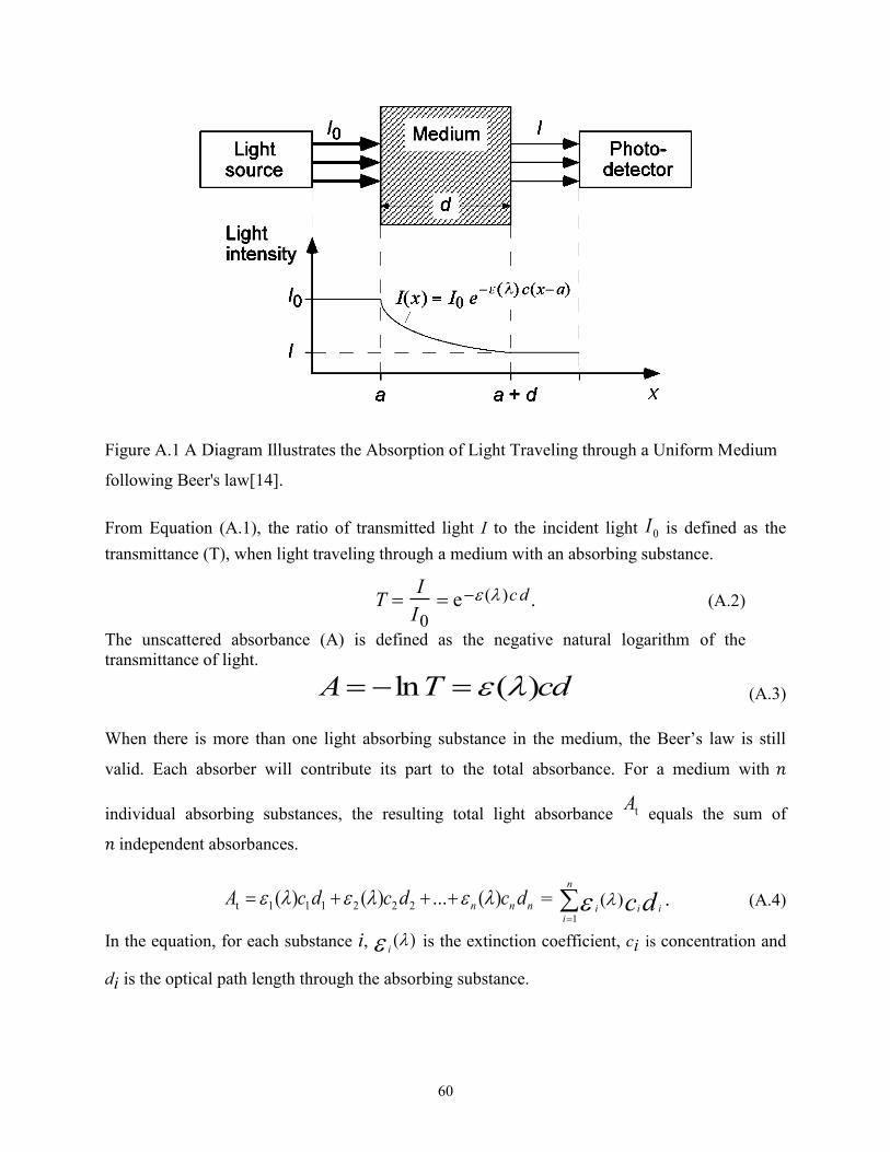
60

Figure A.1 A Diagram Illustrates the Absorption of Light Traveling through a Uniform Medium

following Beer's law[14].

From Equation (A.1), the ratio of transmitted light I to the incident light 0I is defined as the

transmittance (T), when light traveling through a medium with an absorbing substance.

T I

I0 e ( )cd . (A.2)

The unscattered absorbance (A) is defined as the negative natural logarithm of the

transmittance of light.

dcTA )(ln (A.3)

When there is more than one light absorbing substance in the medium, the Beer’s law is still

valid. Each absorber will contribute its part to the total absorbance. For a medium with 𝑛

individual absorbing substances, the resulting total light absorbance tA equals the sum of

𝑛 independent absorbances.

nnn dcdcdcA )(...)()( 222111t =

n

iiii dc

1

)( . (A.4)

In the equation, for each substance i, )( i is the extinction coefficient, ci is concentration and

di is the optical path length through the absorbing substance.

61

Therefore, for a homogeneous medium of multi absorbing substances, when there are different

wavelengths emitted to the substances, Beer’s law can help to determine the light absorbance.

62

Appendix B Beer-Lambert Model in Pulse Oximetry

In pulse oximetry, the oxygen saturation of arterial blood is measured by calculating the light

absorbance of living tissue at two different wavelengths (red light at 660nm and IR light at

940nm) and using the arterial pulsation to differentiate between absorbance of arterial blood and

other absorbers.

According to the Beer’s law in Appendix A, if we assume the optical path length d for the

oxygenated and reduced hemoglobin is the same, with Equation (A.4) and (2.1), the total light

absorbance At that contains only oxygenated and reduced hemoglobin as absorbing substances is

derived as Equation (B.1).

dccSSA )()O1)((O)(22 HbOHb2Hb2HbOt . (B.1)

In this equation, At is expressed for known concentrations of hemoglobin in terms of arterial

oxygen saturation as a fraction, the extinction coefficients of hemoglobin and the length of the

optical path.

During a cardiac cycle, the arterial blood volume increases during the systole and decreases

during the diastole. On the contrary, the blood volume in the veins and capillaries as well as the

volumes of skin, fat, bone, etc., remain relatively constant[13]. Thus, the optical path length d of

Equation (B.1) in the arteries is changed with cardiac cycle and keeps relatively constant in other

tissues. That is to say, in pulse oximetry, the light absorption in arterial blood of the measuring

tissues fluctuates along with cardiac cycles and keeps relatively stable in other areas of the

measuring tissues. Therefore, when the LEDs light from the pulse oximeter passes through the

measuring tissues and finally reaches the PD, a combined signal with pulsatile “alternating

current” (AC) component and non-pulsatile “direct current” (DC) component is generated. The

time varying signal of transmitted light generated at PD is referred to as the plethysmography

(PPG) signal which is the main signal for SpO2 and pulse rate calculation.

Figure B.1 shows the relation of light absorbed and transmitted in a body tissue as a function of

time in pulse oximetry. Usually, the alternating part of the light absorbed by the body tissue does

not exceed 1% to 2% of the constant absorbance of the DC components[14].

63

Figure B.1 PPG Signal of Light Absorption of Body Tissue[36].

The intensity of transmitted light reaching the PD can be expressed as a function of the diameter

d of the arteries. It changes from dmin to dmax in a cardiac cycle. Therefore, if we substitute d

with dmin + ∆d, after derivation, the transmitted light at PD is expressed as a function of Imax

and ∆d.

dccII

])()([

max2HbO2HbOHbHbe

(B.2)

The ratio of the red and IR absorbance of the light signal is introduced to calculate the SpO2.

)/ln(

)/ln(

IRmax,IRmin,

Rmax,Rmin,

IRt,

Rt,

II

II

A

AR (B.3)

Assuming the red light optical path lengths equals the IR light optical path lengths, using

Equation (B.1) and (B.2), we have Equation (B.4).

pO2)]()([)(

O2)]()([)(

IRHbIRHbOIRHb

RHbRHbORHb

2

2

S

SpR

. (B.4)

64

Rewrite Equation (B.4), we get the SpO2 function calculated by ratio R.

%100)]()([)()(

)()(O2

IRHbIRHbORHbORHb

IRHbRHb

22

R

RSp

(B.5)

Where:

• )( RHb is the extinction coefficient of 𝐻𝐻𝑏 at red light

• )( IRHb is the extinction coefficient of 𝐻𝐻𝑏 at IR light

• )( RHbO 2 is the extinction coefficient of 𝑂2𝐻𝑏 at red light

• )( IRHbO 2 is the extinction coefficient of𝑂2𝐻𝑏 at IR light

• R is the ratio obtained from Equation (B.3)

• SpO2 is the arterial oxygen saturation

Therefore, the oxygen saturation in arterial blood is derived theoretically by using Equation (B.3)

and (B.5) with Beer’s law.

For the Beer-Lambert model, the incident light passing through human tissue is simply split into

absorbed light and transmitted light. While in the real situation, some parts of the light are

reflected and others are scattered. Thus, the SpO2 results calculated with Beer-Lambert model

may differ greatly with the actual SpO2 level. Figure B.2 plots the theoretical calibration curve

of the Beer-Lambert model with an empirical calibration curve for comparison. The

Beer−Lambert model tends to give erroneous estimates of the true value of oxygen saturation. In

the figure, if the SpO2 calculated by empirical calibration curve is 100%, with the same R value,

the Beer-Lambert model result is about 93%. This difference between the theoretical curve and

the empirical curve is mainly due to light scattering effects.

65

Figure B.2 Calibration Curves for Pulse Oximeters[37].

design of wireless physiological measurement systems for

Documents