design rules for pumping and metering of highly viscous...

PAPER www.rsc.org/loc | Lab on a Chip

Dow

nloa

ded

by U

nive

rsity

of

Illin

ois

at U

rban

a o

n 27

Sep

tem

ber

2010

Publ

ishe

d on

27

Sept

embe

r 20

10 o

n ht

tp://

pubs

.rsc

.org

| do

i:10.

1039

/C0L

C00

035C

View Online

Design rules for pumping and metering of highly viscous fluids inmicrofluidics†

Sarah L. Perry, Jonathan J. L. Higdon and Paul J. A. Kenis*

Received 18th May 2010, Accepted 26th August 2010

DOI: 10.1039/c0lc00035c

The use of fluids that are significantly more viscous than water in microfluidics has been limited due to

their high resistance to flow in microscale channels. This paper reports a theoretical treatment for the

flow of highly viscous fluids in deforming microfluidic channels, particularly with respect to transient

effects, and discusses the implications of these effects on the design of appropriate microfluidic devices

for highly viscous fluids. We couple theory describing flow in a deforming channel with design

equations, both for steady-state flows and for the transient periods associated with the initial

deformation and final relaxation of a channel. The results of this analysis allow us to describe these

systems and also to assess the significance of different parameters on various deformation and/or

transient effects. To exemplify their utility, we apply these design rules to two applications: (i) pumping

highly viscous fluids for a nanolitre scale mixing application and (ii) precise metering of fluids in

microfluidics.

1. Introduction

Microfluidic approaches have been demonstrated for a wide

variety of applications ranging from virus detection1 and protein

crystallization2 to distillation3 and fuel cells.4 The idea of a ‘‘lab

on a chip,’’ capable of performing ever more complex chemical

and/or biological processes, has been realized in numerous

examples through the integration of multiple unit operations

such as mixing, reaction, separation, and detection on a single

chip. Soft lithography continues to spur the development of

microfluidic technology by providing a fast and easy method for

the rapid prototyping of highly complex networks of channels

with integrated pneumatic valves and peristaltic pumps.5 The

elastomer polydimethylsiloxane (PDMS) has been used in

particular for this purpose because of its ability to replicate

features down to sub-micrometre length scales, such as photo-

lithographically defined channel networks, and the ease by which

the resulting molded layers can be assembled into fully functional

microfluidic chips.6 Additional advantages of PDMS over other

materials include its optical transparency and its elasticity. The

bulk properties of PDMS are equivalent to an incompressible

rubber-like elastic material, with a Young’s modulus E typically

in the range of 0.5 to 4 MPa and a Poisson ratio of s¼ 0.5.7,8 The

pneumatic valves and peristaltic pumps that are now being used

in many microfluidic devices would not be possible without the

high level of deformability of PDMS.9–11 A number of models for

these pneumatic valves and pumps have been reported to

describe and predict their operation.12–14

University of Illinois at Urbana-Champaign, Department of Chemical &Biomolecular Engineering, Urbana, IL, 61801, USA. E-mail: [email protected]; Fax: +1 (217)333-5052; Tel: +1 (217)265-0523

† Electronic supplementary information (ESI) available: Examplecalculations of b for a variety of common microfluidic geometries aswell as details of the curve fitting for the steady-state lag volume. SeeDOI: 10.1039/c0lc00035c

This journal is ª The Royal Society of Chemistry 2010

To date microfluidic applications have been mostly limited to

systems where the fluid viscosities are similar to that of water

because of the challenges associated with pumping highly viscous

and/or non-Newtonian flows. In fact, the pressures that would be

required to drive highly viscous fluids (i.e., �105� more viscous

than water) through a typical microfluidic channel can be

extreme, to the point of exceeding the ability of most pumping

systems used for microfluidics, and/or the capacity of the mate-

rials to sustain such high pressures.15–17 Thus, strategies that

overcome these challenges are needed to enable the pumping of

viscous fluids. In designing a microfluidic device for use with

highly viscous fluids, the single most important consideration is

the viscous resistance to flow. Microfluidic devices are typically

operated under conditions of low Reynolds number flow.

Steady-state operation at low Reynolds number requires ruh/h

� 1 while for unsteady flow we have the additional requirement

that ruh/h � 1, where r is the fluid density, u is the linear flow

velocity, h is the channel height, h is the fluid viscosity, and u is

the frequency of oscillation. For the laminar flows encountered

in microfluidic devices, resistance to flow scales linearly with

viscosity and the length of a channel and with the inverse square

of the cross-sectional area of a channel.18 Thus for a specified

maximum pressure, flow resistance can be decreased by

decreasing the length over which the fluid is flowing, and espe-

cially by enlarging the cross-sectional area of the channel. While

these geometric modifications can be used to facilitate flow of

viscous fluids, the pressures required for flow in a given micro-

fluidic configuration may cause the microfluidic channels to

deform, particularly if elastomeric materials such as PDMS are

used. Channel deformation occurs if the applied pressure exceeds

the stiffness of the material. Channel geometry will vary as

a function of pressure, which in turn varies as a function of

position along the channel. Deformation will be larger at the inlet

of the channel where the pressure is highest, and will decrease

towards the outlet. Previous studies have discussed the effects of

channel deformation in microfluidic configurations, but these

Lab Chip

http://dx.doi.org/10.1039/C0LC00035C

Dow

nloa

ded

by U

nive

rsity

of

Illin

ois

at U

rban

a o

n 27

Sep

tem

ber

2010

Publ

ishe

d on

27

Sept

embe

r 20

10 o

n ht

tp://

pubs

.rsc

.org

| do

i:10.

1039

/C0L

C00

035C

View Online

studies were limited to externally driven, steady-state flow.7,19,20

Channel deformation has also been useful experimentally.

Hardy et al. developed a microfluidic analog for the study of

blood vessels by exploiting the deformability of microchannels in

PDMS.19 Channel deformation as a result of viscous fluid flow in

non-rigid channels also introduces a variety of transient

phenomena that may have a profound effect on the operations

performed on-chip, such as the precise metering of fluids which is

required in many microfluidic applications. For these and several

other on-chip operations, transients as a result of viscous fluid

flow must be taken into account, yet mathematical descriptions

to estimate these transients are presently not available.

This paper develops relevant theory for the flow of highly viscous

fluids in deforming microfluidic channels, particularly with respect

to transient effects, and discusses potential implications on the

design of appropriate microfluidic devices for such highly viscous

fluids. A simple model for a pneumatic valve will be introduced to

characterize the efficiency whereby an applied valve actuation

pressure is translated into a driving force for fluid flow, and scaling

relationships between valve actuation and flow effects will be

identified to aid the design of microfluidic chips for viscous flows.

Next the effects of channel deformation on viscous flows will be

considered. After a steady-state analysis similar to prior work,7,19,20

relevant theory will be derived for the fully transient problem. The

results of the theoretical analysis will then be applied to (i) the

challenges of pumping and precise metering of viscous fluids despite

channel deformation effects, and (ii) the design of a microfluidic

device for the mixing of highly viscous and non-Newtonian fluids.

2. Theory

2.1 The effect of valve membrane actuation on pressure-driven

flow in a rigid channel

The use of integrated microfluidic pneumatic pumps, comprised

of three peristaltic valves in series,2,9,11 has become increasingly

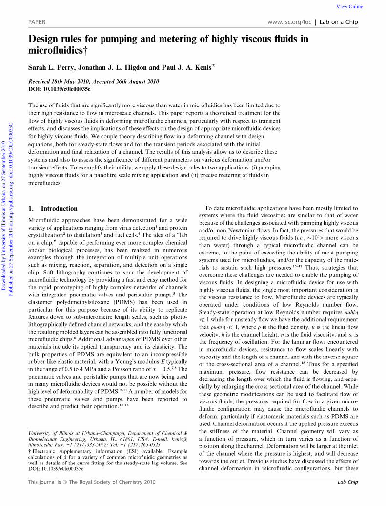
Fig. 1 (a) Depiction of the actuation of a push-down type pneumatic valve. (

valves are actuated in sequence to drive fluid flow. The (100) actuation phase

width w, and height h. Inlet pressure is Pin and pressure at outlet is Pout.

(highlighted in blue) of radius s and thickness a to be deflected a distance hv.

Lab Chip

common, particularly in highly complex microfluidic networks.

This kind of on-chip method to drive fluid flow is desirable

because it enables complex fluid routing while providing better

precision and flexibility than external pressure sources. In

a multilayer microfluidic device, a valve can be defined by an area

where a microfluidic feature from one layer overlaps with that of

a second layer, either above or below. A thin membrane of

elastomeric material separates these two layers and deflects upon

the application of pressure to the valve layer, translating an

externally applied pressure to an internally applied pressure via

deflection of the membrane and eventually sealing off flow in the

fluid layer (Fig. 1a). An on-chip pump can be created by placing

three or more of these valves in series and actuating them in

a sequence to create a peristaltic pumping action (Fig. 1b).9

We use a linearized model valid for small deflection of a thin

membrane to elucidate the effects of various design parameters

on the operation of these valves and the resultant downstream

pressure on the fluid.21 More accurate predictions may be

obtained through detailed non-linear analyses,12–14 however, the

linear model captures the essential scaling needed for the design

of microfluidic valves. For the case of a circular membrane, the

pressure drop associated with this deflection is described by

Pappl � Pin ¼16Ea3z

3ð1� s2Þs4(1)

where the Young’s modulus E and Poisson’s ratio s characterize

the deformability of the valve material, and the valve membrane

is of radius s, thickness a, and experiences an applied pressure

Pappl (Fig. 1d). Deflection of the membrane is taken to be in the z-

direction and is characteristic of the amount of deflection of the

center of the membrane. We assume the valve to be fully actuated

at z ¼ hv, the height of the valve chamber. Within the valve

chamber, we assume that the only pressure losses are those due to

deflection of the membrane, resulting in a pressure in the valve

chamber of Pin.

b) Depiction of a 3-phase peristaltic pump where a set of three pneumatic

is shown. (c) Schematic depiction of a microfluidic channel of length L,

(d) Depiction of a theoretical pneumatic valve with circular membrane

Applied pressure is Pappl and pressure inside of the valve is Pin.



Dow

nloa

ded

by U

nive

rsity

of

Illin

ois

at U

rban

a o

n 27

Sep

tem

ber

2010

Publ

ishe

d on

27

Sept

embe

r 20

10 o

n ht

tp://

pubs

.rsc

.org

| do

i:10.

1039

/C0L

C00

035C

View Online

We can use eqn (1) to consider the pressure driving force

available for pumping after valve actuation, assuming a pressure

difference across the valve of DP ¼ Pappl – Pin. We can then

normalize eqn (1) by the applied pressure Pappl and define

a parameter a that describes the pressure losses associated with

the actuation, or stiffness, of the valve.

a ¼ Pappl � Pin

Pappl

¼ 16Ea3hv

3Papplð1� s2Þs 4(2)

From eqn (2) it follows that the term a approaches zero when

the pressure losses due to the valve are small. We can thus define

the case where actuation of a pneumatic valve has a negligible

effect on the pressures associated with fluid flow in the limit of

a / 0. This limit can be approached physically by modifying the

stiffness (E/Pappl) and/or the geometry (a3hv/s4) of the valve.

When the ratio of E/Pappl is small, the applied pressure is able to

easily overcome the resistance of the valve material to defor-

mation. The thickness of the valve membrane a along with the

extent of deflection hv can be modified along with the radius of

the valve s in order to minimize the geometric term a3hv/s4.

We now have a method to determine Pin, the pressure available

for pumping at the inlet of a microfluidic channel, whether it is

directly applied by an external source or determined using eqn

(1). Let us now consider fluid flow in a long microfluidic channel

of length L, width w, and height h (Fig. 1c). Typically micro-

fluidic channels have a low aspect ratio such that w [ h, and the

channel can be treated effectively as an infinite slit. Furthermore,

the small dimensions of these channels lead to a small Reynolds

number and thus laminar flow. The driving pressure Pin is

dissipated over the length of the channel to an outlet pressure of

Pout. The z-axis is taken to be in the direction of flow along the

length of the channel.

The hydrodynamics of viscous flow in an infinite slit of rigid

geometry are well understood and an expression for the volu-

metric flow rate _V can be easily derived in terms of the channel

dimensions, pressure gradient dP/dz, and fluid viscosity h.18

_V ¼ �h3w

12h

dP

dz(3)

For a channel of set dimensions, which we term as a ‘rigid’

channel, a linear pressure drop (DP/L) is realized over the length

of the channel with DP¼ Pin� Pout. Note that since the pressure

front is assumed to transfer instantaneously through an incom-

pressible fluid, our result is valid for all times.

2.2 The effect of channel deformation on viscous flow

In using elastomeric materials, deformation of the bulk material

defining a channel is possible. Thus, rather than considering

a thin membrane as in Section 2.1, we now consider deformation

of an infinite slab subject to an applied surface pressure.

2.2.1 Steady-state viscous flow in a deformed channel.

Deformation of the channel can be modeled as a distributed

pressure over an infinite slab.22 For a typical PDMS device on

a stiff glass substrate, it is only necessary to consider deformation

of the top wall of the microfluidic channel so long as the aspect

ratio of the device does not approach unity (also a requirement


for viscous flow in an infinite slit).7,22 The maximum deformation

of a slab can be written in terms of the ratio of pressure to

Young’s modulus P/E, a characteristic length which for a low

aspect ratio channel is the width w, and a proportionality

constant c which takes into consideration the geometry of the

deforming area and is of order of magnitude �1.7,19,22 Thus,

Dhmax ¼cPwð1þ sÞ

E(4)

Previous work has demonstrated that this deformation is

parabolic across the width of a microfluidic channel.7,19 Owing to

the nonlinear dependence on h in eqn (3), the change in _V with

variable h cannot be captured by using an average value for h.

Nonetheless, it is convenient to compute hDhi ¼ 2/3Dhmax, as has

been done previously,7,19 and thus we can write an expression for

an effective height h(z) along the length of the channel as

a function of P(z) and the initial channel height h0. We note that

the relevant coefficient for the effective height may differ from 2/

3 in practice.

hðzÞ ¼ h0

�1þ 2cPðzÞwð1þ sÞ

3Eh0

�(5)

Substituting this function for the channel height into our

expression for volumetric flow rate from eqn (3), we generate the

following expression for the volumetric flow rate in a deformed

channel as a function of the pressure drop along the length of the

channel.

_V ¼ �h30w

12h

�1þ 2cPwð1þ sÞ

3Eh0

�3vP

vz(6)

At steady-state the volumetric flow rate is constant, and we can

integrate eqn (6) over the length of the channel assuming an inlet

pressure of Pin and letting Pout ¼ 0. Combining the integrated

form of eqn (6) with eqn (3) and defining a non-dimensional

parameter b which characterizes the tendency of a channel to

deform, we obtain an analytical form of the steady-state volu-

metric flow rate for a deformed channel in terms of the volu-

metric flow rate for a rigid channel and a correction term that

depends on b. The rigid solution can be obtained by setting b¼ 0.

_V ssdef ¼ _V rigid

�1þ 3b

2þ b2 þ b3

4

�(7)

where

b ¼ 2cPinwð1þ sÞ3Eh0

¼ 2Dhmax

h0

(8)

b describes the tendency of the material to deform given the ratio

Pin/E. The larger the applied pressure compared to the Young’s

modulus, the larger the deformation. For the purposes of the

analyses presented here—particularly given the approximation

of flow in an infinite slit—we will only examine behavior over the

range of b < 3. We established this threshold for our analysis

based on the aspect ratio of the deformed device such that the

assumption of an infinite slit is still valid. For example, if we

consider a channel of width w¼ 100 mm and initial height h0¼ 10

mm our initial aspect ratio is 0.1, indicating an order of magni-

tude difference between the two dimensions. However, for the

Lab Chip


Dow

nloa

ded

by U

nive

rsity

of

Illin

ois

at U

rban

a o

n 27

Sep

tem

ber

2010

Publ

ishe

d on

27

Sept

embe

r 20

10 o

n ht

tp://

pubs

.rsc

.org

| do

i:10.

1039

/C0L

C00

035C

View Online

case of b ¼ 3, channel deformation results in an average channel

height of h¼ 40 mm and an aspect ratio of 0.4, indicating that the

height and width of the channel are of nearly the same order.

To obtain an expression for P(z) we integrate eqn (6) and

substitute eqn (7):

PðzÞ ¼ Pin

b

��z

L1� ð1þ bÞ4

�þ ð1þ bÞ4

� �1=4

�1

�(9)

Owing to the deformation of the channel, we see a 4th root

decay of pressure along the channel length rather than the linear

dependence seen in the rigid case (Fig. 2a). In the limit of small b,

eqn (9) reduces to the rigid limit described by eqn (3).

Combining the expressions for channel height in eqn (5) and

pressure in eqn (9), we may integrate over the length of the

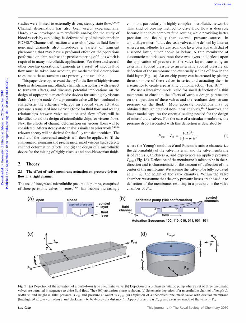
Fig. 2 Plots of (a) steady-state pressure profiles for different values of b alon

than the linear rigid case at all points in the channel. (b) Steady-state volumetr

the deformation parameter b. (c) The change in the channel volume normalized

curve can be approximated as 0.5b, as shown.

Lab Chip

channel to find the change in volume Vswell due to the

deformation.

Vswell ¼ Vrigid

"4

5

1� ð1þ bÞ5

1� ð1þ bÞ4

!� 1

#(10)

Having developed the mathematics behind steady-state flow in

a deformed channel, let us examine the physical meaning behind

some of these results. As described in eqn (9), and shown in Fig. 2a,

the pressure profile along the length of the channel is nonlinear,

which corresponds to the channel deformation. At the beginning

of the channel where the large applied pressure results in a large

deformation, relatively small pressure losses occur resulting in

pressure gradients that are lower than for the purely rigid case.

g the microfluidic channel. Pressures in the deformed channels are larger

ic flow rate normalized by the flow rate in a rigid channel as a function of

by the rigid channel volume as a function of b. In the limit of small b this



Dow

nloa

ded

by U

nive

rsity

of

Illin

ois

at U

rban

a o

n 27

Sep

tem

ber

2010

Publ

ishe

d on

27

Sept

embe

r 20

10 o

n ht

tp://

pubs

.rsc

.org

| do

i:10.

1039

/C0L

C00

035C

View Online

However, near the end of the channel where deformations are

small, we observe much steeper pressure gradients. Both channel

deformation and steeper pressure gradients combine to enhance

the volumetric flow rate. At steady-state, the most significant

result of channel deformation is the 3rd order polynomial depen-

dence of the volumetric flow rate on b described in eqn (7) and

plotted in Fig. 2b. While for small deformations this effect can be

neglected, a dramatic increase in flow rates is seen at larger

deformations. For example, at a value of b ¼ 1, typical for many

microfluidic systems, the volumetric flow rate resulting from the

deformed channel is 375% higher than the corresponding flow rate

expected for a rigid channel. (See the ESI† for calculated values of

b as a function of various microfluidic device geometries.) An

additional effect of channel deformation is an increase in the total

volume of the channel. While the precise dependence of the swell

volume with respect to deformation given in eqn (10) is compli-

cated, one can approximate the relationship depicted in Fig. 2c as

Vswell/Vrigid z 0.5b from a Taylor series expansion for small b. The

effect of the swell volume should have little impact on steady-state

operation of a device but can become significant when considering

unsteady effects where the channel volume changes with time,

causing the inlet and outlet volumetric flow rates to be unequal.

2.2.2 Unsteady viscous flow in a deforming channel. To

examine unsteady viscous flow, we begin with a mass balance

relating changes in h to _V .

vh

vt¼ �1

w

v _V

vz(11)

Assuming that h changes slowly with z, we can combine eqn (11)

with the expression for volumetric flow rate, eqn (6), and write an

equation for the channel pressure P as a function of z and t.

vP

vt¼ v

vz

"Eh3

0

8chwð1þ sÞ

�1þ 2cPwð1þ sÞ

3Eh0

�3vP

vz

#(12)

The initial condition is P¼ 0 at t¼ 0, and boundary conditions

are P ¼ Pin at z ¼ 0; P ¼ 0 at z ¼ L.

The expression is non-dimensionalized using the core vari-

ables: applied pressure Pin, the channel length L, and the fluid

viscosity h. These variables are chosen because they are physical

parameters which can be easily controlled and which define

resultant quantities in our system such as volumetric flow rate.

The non-dimensional forms of the variables are:

U ¼ P

Pin

; Z ¼ z

L; s ¼ tPin

h(13)

Applying this non-dimensionalization and the definition for

b from eqn (8), we obtain the partial differential equation:

vU

vs¼ v

vZ

�gð1þ bUÞ3 vU

vZ

�(14)

The non-dimensionalized initial condition is U¼ 0 at s¼ 0, the

boundary conditions are U¼ 1 at Z¼ 0; U¼ 0 at Z¼ 1, and g is

defined as:

g ¼ 1

12b

�h0

L

�2

(15)

The form of eqn (14) is analogous to that of a diffusion

equation with a variable diffusivity of g(1 + bU)3.


Because g is related to this variable diffusivity we can use it to

define a dimensionless diffusive time s*.

s* ¼ gs ¼ gPint

h(16)

With this definition we obtain the modified partial differential

equation:

vU

vs*¼ v

vZ

�ð1þ bUÞ3 vU

vZ

�(17)

The modified non-dimensionalized initial condition is U¼ 0 at

s*¼ 0, and the boundary conditions are U¼ 1 at Z¼ 0; U¼ 0 at

Z ¼ 1.

The boundary value problem defined by eqn (17) with asso-

ciated initial and boundary conditions was solved numerically in

MATLAB (Mathworks Inc., version 7.6.0.324).23 A variable grid

mesh was used to capture the increasingly steep behavior of the

function near the outlet at Z ¼ 1. At long times the solution is

observed to approach the steady-state values predicted from the

analytical solutions. Results are shown below for b ¼ 1, which is

typical for a PDMS channel (Fig. 3).

As mentioned previously, the form of the boundary value

problem is the same as nonlinear diffusion in a channel. It is

intuitive to think of a large slug of concentration entering the

channel and then slowly diffusing along its length. In an analo-

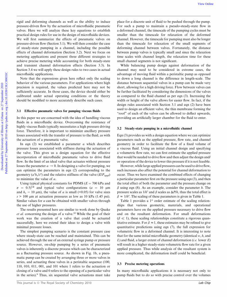
gous fashion, the pressure profile within the channel develops

first as a sharp impulse at the entrance of the channel and then

spreads down the length of the channel as deformation occurs

and steady-state is reached (Fig. 3a). From eqn (5) the channel

height scales directly with pressure. Deformation or ‘‘inflation’’

of the channel due to the applied pressures thus matches the

changes in pressure profile.

The initial impulse of pressure also translates to the initial

generation of steep pressure gradients. These steep gradients

allow for rapid filling at the start of the deforming channel.

However, the pressure gradients take time to propagate down the

length of the channel, resulting in a lag between the start of flow

at the inlet and the observation of flow at the outlet. This lag time

can be more clearly observed by examining a plot of normalized

volumetric flow rate at the outlet as a function of time (Fig. 3c).

A similar analysis can be used to examine the case where

a deformed channel is allowed to relax in the absence of an inlet

pressure. In this instance the pressure driving force for flow

comes from the deformed channel as it relaxes. Referring again

to the diffusion analogy, the steady-state concentration (or in our

case pressure) profile slowly decays to zero as material diffuses to

the outlet (Fig. 3b). However, the driving force for this diffusion

decreases with time as the concentration profile levels out in the

channel. Translating this analogy to pressure and fluid flow, we

observe an initially high flow rate at the outlet that asymptoti-

cally approaches zero as the pressure gradients in the channel

become negligible (Fig. 3c).

The trends in the pressure driving force for flow are very

different between the filling and emptying cases. For the filling

case there is a constant inlet pressure that then propagates along

the length of the channel. This results in a fairly rapid approach

to steady-state. However, for the emptying case the pressure

driving force decreases with time, asymptotically approaching

Lab Chip


Fig. 3 Results from the MATLAB simulation of the fully transient problem of pressure-driven viscous flow in a deforming channel using parameters that

are typical for flow in a PDMS channel giving a value of b¼ 1. Here the channel is deforming to reach a steady-state profile over time. (a) Dimensionless

pressure over the length of the channel Z at intervals from s*¼ 0 to s*¼ 0.1 for the filling case, and (b) over intervals from s*¼ 0 to s*¼ 1.0 for the emptying

case. (c) Volumetric flow rate at the outlet normalized by the flow rate for a rigid channel as a function of time for both filling and emptying. (d) Time to fill

or empty 99% of the channel volume for the transient filling and emptying cases, respectively, as normalized to the rigid case.

Dow

nloa

ded

by U

nive

rsity

of

Illin

ois

at U

rban

a o

n 27

Sep

tem

ber

2010

Publ

ishe

d on

27

Sept

embe

r 20

10 o

n ht

tp://

pubs

.rsc

.org

| do

i:10.

1039

/C0L

C00

035C

View Online

zero. A comparison of the outlet volumetric flow rate curves for

the two cases in Fig. 3c shows that the time to reach steady-state

is significantly longer for the emptying case.

We can also examine how the rate at which a deforming

channel approaches steady-state varies with b (Fig. 3d). We

characterize the time for filling as the swell volume divided by the

volumetric flow rate. If we then analyze the b dependence of this

filling time we obtain the result:

tfillzVswell

_Vz

bP

ð1þ bPÞ3(18)

In the limit of small b, the filling time scales linearly with b. This

relationship is the result of roughly linear increases in the swell

Lab Chip

volume that dominates over negligible increases in the volumetric

flow rate. However, in the limit of large b, the time scales as the

inverse square of b as increases in the channel volume are balanced

by the geometric increases in the volumetric flow rate.

While it is more difficult to extract trends for the emptying case,

Fig. 3c and d clearly show that the time for the emptying case to

reach steady-state is significantly longer than that of the filling

case. Despite this difference, similar trends with b are observed.

3. Design rules

In Section 2 a theoretical analysis of various aspects of the

microfluidic system yielded key equations to describe flow in



Dow

nloa

ded

by U

nive

rsity

of

Illin

ois

at U

rban

a o

n 27

Sep

tem

ber

2010

Publ

ishe

d on

27

Sept

embe

r 20

10 o

n ht

tp://

pubs

.rsc

.org

| do

i:10.

1039

/C0L

C00

035C

View Online

rigid and deforming channels as well as the ability to induce

pressure-driven flow by the actuation of microfluidic pneumatic

valves. Here we will analyze these key equations to establish

practical design rules for use in the design of microfluidic devices.

We will first summarize the effects of pneumatic valves on

pressure-driven flow (Section 3.1). We will then consider the case

of steady-state pumping in a channel, including the possible

effects of channel deformation (Section 3.2). Next we focus on

metering applications and present three different strategies to

achieve precise metering while accounting for both steady-state

and transient channel deformation effects (Section 3.3). In

Section 3.4 we will apply these design rules to two cases in actual

microfluidic applications.

Note that the expressions given here reflect only the scaling

behavior of the various parameters. For applications where high

precision is required, the values predicted here may not be

sufficiently accurate. In those cases, the device should either be

calibrated under actual operating conditions or the theory

should be modified to more accurately describe such cases.

3.1 Effective pneumatic valves for pumping viscous fluids

In this paper we are concerned with the idea of handling viscous

fluids in a microfluidic device. Overcoming the resistance of

highly viscous fluids typically necessitates a high pressure driving

force. Therefore, it is important to minimize ancillary pressure

losses associated with the transfer of pressure to the fluid, as with

the actuation of a pneumatic valve.

In eqn (2) we established a parameter a which describes

pressure losses associated with stiffness during the actuation of

the valve. This gives us a design equation for the effective

incorporation of microfluidic pneumatic valves to drive fluid

flow. In the limit of an ideal valve that actuates without pressure

losses the parameter a / 0. In designing a valve for pumping, we

can optimize the parameters in eqn (2) corresponding to the

geometry (a3hv/s4) and the relative stiffness of the valve (E/Pappl)

to minimize the value of a.

Using typical physical constants for PDMS (E ¼ 700 kPa and

s ¼ 0.5)7,8 and typical valve configurations (a ¼ 10 mm

and hv ¼ 10 mm), the value of a is small (<0.05) for valve sizes

s > 100 mm at actuation pressures as low as 10 kPa (1.45 psi).

Similar values for a can be obtained with smaller valves through

the use of higher pressures.

The results presented here are similar to work done by Quake

et al. concerning the design of a valve.12 While the goal of their

work was the creation of a valve that could be actuated

successfully, here we extend their ideas to design a valve with

minimal pressure losses.

The simplest pumping scenario is the constant pressure case

where steady-state can be reached and maintained. This can be

achieved through the use of an external syringe pump or pressure

source. However, on-chip pumping by a series of pneumatic

valves is inherently a discrete process which can be characterized

as a fluctuating pressure source. As shown in Fig. 1b, a pneu-

matic pump can be created by arranging three or more valves in

series, and actuating these valves in a peristaltic sequence (100,

110, 010, 011, 001, and 101 where 1 refers to the actuation or

closing of a valve and 0 refers to the opening of a particular valve

in the series).9 Thus, six sequential valve actuations must take


place for a discrete unit of fluid to be pushed through the pump.

For such a pump to maintain a pseudo-steady-state flow in

a deformed channel, the timescale of the pumping cycles must be

smaller than the timescale for relaxation of the deformed

channel. However, the timescale for pumping must also be longer

than the timescale for relaxation of the small segments of

deforming channel between valves. Fortunately, the distance

between pump valves is typically small and since the relaxation

time scales with channel length, the relaxation time for these

small channel segments is not significant.

While balancing pump design against deformation of the

channel may need to be considered in extreme cases, the

advantage of moving fluid within a peristaltic pump as opposed

to down a long channel is the difference in length-scale. The

distance between sequential valves in a pump can be made very

short, allowing for a high driving force. Flow between valves can

be further facilitated by considering the dimensions of the valves

as compared to the fluid channel as per eqn (3). Increasing the

width or height of the valve allows for easier flow. In fact, if the

design rules associated with Section 3.1 and eqn (2) have been

used to design an efficient valve, the thin membrane forming the

‘‘roof’’ of each of the valves can be allowed to deflect upwards,

providing an artificially larger chamber for the fluid to enter.

3.2 Steady-state pumping in a microfluidic channel

Eqn (3) provides us with a design equation where we can optimize

parameters such as the applied pressure, flow rate, and channel

geometry in order to facilitate the flow of a fixed volume of

a viscous fluid. Using an initial channel design and specifying

a volumetric flow rate, we can first estimate the applied pressure

that would be needed to drive flow and then adjust the design and/

or operation of the device to lower this pressure if it is not feasible.

However, while large applied pressures can be used to drive flow,

such increases also affect the potential for channel deformation to

occur. Thus we have examined the combined effects of changing

a particular parameter first on the pressure using eqn (3), and then

the total effect of both the parameter and the pressure change on

b using eqn (8). As an example, consider the parameter h. The

pressure scales as 1/h3 and b scales as DP/h, thus the total effect is

b z 1/h4. The scaling of these parameters is given in Table 1.

Table 1 provides a 1st order estimate of the scaling relation-

ships that various geometric, materials, and operational

parameters have on the applied pressure necessary to drive flow

and on the resultant deformation. For small deformations

(b � 1), these scaling relationships constitute a rigorous quan-

titative estimate. For b z1, these estimates may be refined to give

quantitative predictions using eqn (7), the full expression for

volumetric flow in a deformed channel. It is interesting to note

that for the same initial microfluidic geometry (identical w, h, and

L) and fluid, a larger extent of channel deformation (i.e. lower E)

will result in a higher steady-state volumetric flow rate for a given

applied pressure. Thus while analysis of the resultant system is

more complicated, the deformation itself could be beneficial.

3.3 Precise metering operations

In many microfluidic applications it is necessary not only to

pump fluids but to do so with precise control over the volumes

Lab Chip


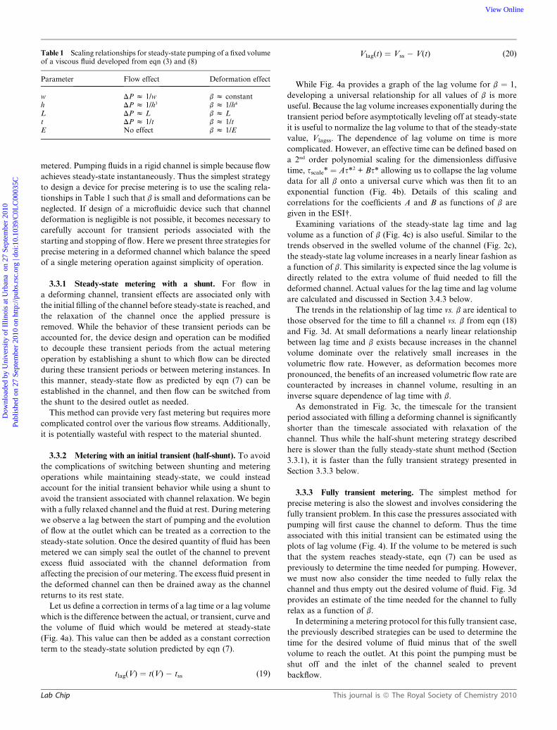
Table 1 Scaling relationships for steady-state pumping of a fixed volumeof a viscous fluid developed from eqn (3) and (8)

Parameter Flow effect Deformation effect

w DP z 1/w b z constanth DP z 1/h3 b z 1/h4

L DP z L b z Lt DP z 1/t b z 1/tE No effect b z 1/E

Dow

nloa

ded

by U

nive

rsity

of

Illin

ois

at U

rban

a o

n 27

Sep

tem

ber

2010

Publ

ishe

d on

27

Sept

embe

r 20

10 o

n ht

tp://

pubs

.rsc

.org

| do

i:10.

1039

/C0L

C00

035C

View Online

metered. Pumping fluids in a rigid channel is simple because flow

achieves steady-state instantaneously. Thus the simplest strategy

to design a device for precise metering is to use the scaling rela-

tionships in Table 1 such that b is small and deformations can be

neglected. If design of a microfluidic device such that channel

deformation is negligible is not possible, it becomes necessary to

carefully account for transient periods associated with the

starting and stopping of flow. Here we present three strategies for

precise metering in a deformed channel which balance the speed

of a single metering operation against simplicity of operation.

3.3.1 Steady-state metering with a shunt. For flow in

a deforming channel, transient effects are associated only with

the initial filling of the channel before steady-state is reached, and

the relaxation of the channel once the applied pressure is

removed. While the behavior of these transient periods can be

accounted for, the device design and operation can be modified

to decouple these transient periods from the actual metering

operation by establishing a shunt to which flow can be directed

during these transient periods or between metering instances. In

this manner, steady-state flow as predicted by eqn (7) can be

established in the channel, and then flow can be switched from

the shunt to the desired outlet as needed.

This method can provide very fast metering but requires more

complicated control over the various flow streams. Additionally,

it is potentially wasteful with respect to the material shunted.

3.3.2 Metering with an initial transient (half-shunt). To avoid

the complications of switching between shunting and metering

operations while maintaining steady-state, we could instead

account for the initial transient behavior while using a shunt to

avoid the transient associated with channel relaxation. We begin

with a fully relaxed channel and the fluid at rest. During metering

we observe a lag between the start of pumping and the evolution

of flow at the outlet which can be treated as a correction to the

steady-state solution. Once the desired quantity of fluid has been

metered we can simply seal the outlet of the channel to prevent

excess fluid associated with the channel deformation from

affecting the precision of our metering. The excess fluid present in

the deformed channel can then be drained away as the channel

returns to its rest state.

Let us define a correction in terms of a lag time or a lag volume

which is the difference between the actual, or transient, curve and

the volume of fluid which would be metered at steady-state

(Fig. 4a). This value can then be added as a constant correction

term to the steady-state solution predicted by eqn (7).

tlag(V) ¼ t(V) � tss (19)

Lab Chip

Vlag(t) ¼ Vss � V(t) (20)

While Fig. 4a provides a graph of the lag volume for b ¼ 1,

developing a universal relationship for all values of b is more

useful. Because the lag volume increases exponentially during the

transient period before asymptotically leveling off at steady-state

it is useful to normalize the lag volume to that of the steady-state

value, Vlagss. The dependence of lag volume on time is more

complicated. However, an effective time can be defined based on

a 2nd order polynomial scaling for the dimensionless diffusive

time, sscale* ¼ As*2 + Bs* allowing us to collapse the lag volume

data for all b onto a universal curve which was then fit to an

exponential function (Fig. 4b). Details of this scaling and

correlations for the coefficients A and B as functions of b are

given in the ESI†.

Examining variations of the steady-state lag time and lag

volume as a function of b (Fig. 4c) is also useful. Similar to the

trends observed in the swelled volume of the channel (Fig. 2c),

the steady-state lag volume increases in a nearly linear fashion as

a function of b. This similarity is expected since the lag volume is

directly related to the extra volume of fluid needed to fill the

deformed channel. Actual values for the lag time and lag volume

are calculated and discussed in Section 3.4.3 below.

The trends in the relationship of lag time vs. b are identical to

those observed for the time to fill a channel vs. b from eqn (18)

and Fig. 3d. At small deformations a nearly linear relationship

between lag time and b exists because increases in the channel

volume dominate over the relatively small increases in the

volumetric flow rate. However, as deformation becomes more

pronounced, the benefits of an increased volumetric flow rate are

counteracted by increases in channel volume, resulting in an

inverse square dependence of lag time with b.

As demonstrated in Fig. 3c, the timescale for the transient

period associated with filling a deforming channel is significantly

shorter than the timescale associated with relaxation of the

channel. Thus while the half-shunt metering strategy described

here is slower than the fully steady-state shunt method (Section

3.3.1), it is faster than the fully transient strategy presented in

Section 3.3.3 below.

3.3.3 Fully transient metering. The simplest method for

precise metering is also the slowest and involves considering the

fully transient problem. In this case the pressures associated with

pumping will first cause the channel to deform. Thus the time

associated with this initial transient can be estimated using the

plots of lag volume (Fig. 4). If the volume to be metered is such

that the system reaches steady-state, eqn (7) can be used as

previously to determine the time needed for pumping. However,

we must now also consider the time needed to fully relax the

channel and thus empty out the desired volume of fluid. Fig. 3d

provides an estimate of the time needed for the channel to fully

relax as a function of b.

In determining a metering protocol for this fully transient case,

the previously described strategies can be used to determine the

time for the desired volume of fluid minus that of the swell

volume to reach the outlet. At this point the pumping must be

shut off and the inlet of the channel sealed to prevent

backflow.



Fig. 4 Results from the MATLAB simulation of the fully transient problem of pressure-driven viscous flow in a deforming channel. (a) The volume

passing through the outlet normalized by the volume of a rigid channel as a function of time for the transient case and for hypothetical instantaneous

steady-state flow for b ¼ 1. (b) A plot of normalized lag volume vs. a scaled dimensionless time. The solid curve is an exponential fit to the data which is

universal for all b. (c) The steady-state lag time normalized by the time for flow in the rigid case to accomplish a total rigid channel volume and the

steady-state lag volume normalized to the channel volume for metering as a function of b.

Dow

nloa

ded

by U

nive

rsity

of

Illin

ois

at U

rban

a o

n 27

Sep

tem

ber

2010

Publ

ishe

d on

27

Sept

embe

r 20

10 o

n ht

tp://

pubs

.rsc

.org

| do

i:10.

1039

/C0L

C00

035C

View Online

3.4 Applications of the design rules

Thus far we have described the physics behind various

phenomena present in a microfluidic device and developed

associated design rules. Let us now apply these design rules to

two examples in actual microfluidic applications: (i) a micro-

fluidic device for mixing highly viscous fluids and (ii) the precise

metering of fluid using a pneumatic on-chip pump over a range of

fluid viscosities.

3.4.1 Creating a mixer for highly viscous fluids. Microfluidic

applications involving highly viscous fluids have lagged behind

their less viscous counterparts mostly because of the difficulty in


flowing high viscosity fluids on the microscale. The simple scaling

relationships that resulted from the work presented above

(Table 1) enable the design of microfluidic devices capable of

driving flow for fluids that are not only highly viscous but also

non-Newtonian. We coupled these design rules with strategies

for mixing to create a microfluidic mixer capable of operating

with fluids of both differing and high viscosities.2

The majority of microfluidic mixers, such as the ring mixer

devised by the Quake group11,24,25 or the herringbone mixer

devised by Stroock and coworkers,26,27 require driving flow over

relatively long distances. These mixer designs have difficulty

operating with higher viscosity fluids, especially when trying to

Lab Chip


Dow

nloa

ded

by U

nive

rsity

of

Illin

ois

at U

rban

a o

n 27

Sep

tem

ber

2010

Publ

ishe

d on

27

Sept

embe

r 20

10 o

n ht

tp://

pubs

.rsc

.org

| do

i:10.

1039

/C0L

C00

035C

View Online

mix fluids of significantly different viscosities. Thus instead of

striving to establish complex flow patterns in a long channel, we

chose to develop a mixing strategy that is compatible with the

need to pump higher viscosity fluids (Fig. 5). Previously we

reported on the operation and application of this device to mix

a viscous lipid (monoolein) and an inviscid aqueous solution.2

Here we describe how the scaling relationships were used in its

design. The viscous fluid mixer is composed of three microfluidic

chambers connected by small microfluidic channels. In this two-

layer PDMS device, isolation valves are located both over the

inlet lines used to fill the device and over the channels connecting

each of the three chambers. Large microfluidic injection valves

are also located over each of the three large chambers containing

the fluids to be mixed. These injection valves are used to pump

fluid from one compartment to another while the various isola-

tion valves on the connecting channels control the direction of

fluid flow. Mixing is achieved by first driving flow in a linear

fashion from the side chambers into the center chamber through

all of the available injection lines. Two recirculating loops of flow

are then created on the two halves of the device by using first one

injection line for flow to the side chambers, then two lines to

return to the center chamber, and then again a single line to refill

the side chambers. These straight-line and recirculating flow

patterns are repeated to drive fluid mixing in a tendril–whorl

fashion.28 We used this mixer to prepare self-assembling

aqueous/lipid mesophases where the viscosity of the initial

aqueous and lipid solutions differed by a factor of �30 (2.45 �10�2 Pa s for the lipid phase versus 7.98 � 10�4 Pa s for the

aqueous phase). Furthermore, the resulting mixture had

a viscosity �105 times larger than that of water (�48.3 Pa s at

a shear rate of 71.4 s�1) and displayed non-Newtonian fluid

behavior. These mesophases are of interest particularly in

structural biology applications, including membrane protein

crystallization.29

Fig. 5 Optical micrograph of a microfluidic mixer designed to mix

highly viscous fluids or fluids of vastly different viscosities. Pneumatic

valves are outlined in green and are located as isolation valves over inlet

lines leading into each of three larger chambers as well as over lines

connecting the three chambers. Valves used to drive fluid flow are located

over each of the three large chambers. (a) The injection of an aqueous

solution from the side chambers into the center chamber containing

a highly viscous lipid. (b) Injection of fluid from the center chamber to the

side chambers through a single injection line. See ref. 2 for more details on

the mixing sequence.2

Lab Chip

In designing this microfluidic mixing device, the first challenge

that needed to be overcome was pumping fluids with viscosities

several orders of magnitude higher than water. We were able to

counter this increased viscous resistance by designing the

geometry of our device based on the design rules in Table 1, such

that operational parameters, including the applied pressure to

drive flow, could be optimized (i.e. minimized to attainable

pressure levels). Instead of trying to pump a highly viscous fluid

over a long distance in a narrow channel, we configured the mixer

such that (i) the distance for flow L is short and (ii) the width w of

the device is large. The use of large fluid chambers allowed us to

minimize the distance over which fluid was pumped in a narrow

channel. These large chambers have the added benefit of

ensuring, as per the scaling relationships associated with the

parameter a in eqn (2), that the pneumatic valves located over

each chamber are able to efficiently drive flow without significant

pressure losses. Including these chamber valves in our design

provided two additional benefits: (i) whereas the actual height of

the fluid chambers in our device is a constant, the presence of an

easily deflectable valve over each of the chambers allows us to

effectively consider each of the chambers as having a much larger

height than was initially designed. The design rules derived here

(Table 1) show that the required pressure to drive viscous flow

scales with the cube of the channel height, meaning that even

small increases in height significantly decrease the pressure

needed to drive fluid flow. (ii) We were able to pump the entire

contents of each individual chamber with a single actuation,

rather than by repeated pumping steps to move smaller portions

of fluid around. (iii) Lastly, we were also able to operate our

device relatively slowly such that adverse effects of the increased

fluid viscosity which we had not overcome through device design

could be compensated for by accepting a lower flow rate. The

mesophase that is formed upon mixing in this study also dis-

played viscoelastic behavior. An additional benefit of the

decreased flow rate was adequate compensation for the relaxa-

tion timescales associated with the fluid.

Based on the geometry of the device and the large applied

pressures needed to drive flow, our calculated value of b z 2

indicates that deformation of the channels connecting the

compartments will be significant. As discussed previously

(Section 2.2), this kind of deformation decreases pressure losses

along the length of a channel and can provide further benefits for

moving highly viscous fluids between chambers. While defor-

mation is only an issue for the short channels connecting the

larger microfluidic chambers, the short length of these channels

means that the lag time and volume will be relatively small

compared to the total volume of fluid to be pumped. Addition-

ally, relaxation of the extra volume in these channels is not

a concern because microfluidic isolation valves over each of these

channels are actuated as part of the mixing sequence and will

expel fluid remaining in the channel.

3.4.2 Peristaltic fluid metering

The case of a rigid channel. The ability to precisely meter out

picolitre-scale (or smaller) quantities of fluids has been clearly

demonstrated in microfluidic devices, typically by the peristaltic

actuation of a series of pneumatic valves.24 This method typically

assumes that the volume of fluid displaced under the valve will be

moved down the channel without losses due to channel



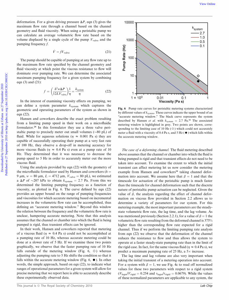
Fig. 6 Pump rate curves for peristaltic metering systems characterized

by different values of ksystem. These curves indicate the upper bound of an

‘‘accurate metering window.’’ The black curve represents the system

described by Hansen et al. with ksystem ¼ 2.7 Pa.24 The associated

metering window is highlighted in grey. Two points are shown, corre-

sponding to the limiting case of 10 Hz (>) which could not accurately

meter a fluid with a viscosity of 0.4 Pa s, and 5 Hz (A) which falls within

the accurate metering window.

Dow

nloa

ded

by U

nive

rsity

of

Illin

ois

at U

rban

a o

n 27

Sep

tem

ber

2010

Publ

ishe

d on

27

Sept

embe

r 20

10 o

n ht

tp://

pubs

.rsc

.org

| do

i:10.

1039

/C0L

C00

035C

View Online

deformation. For a given driving pressure DP, eqn (3) gives the

maximum flow rate through a channel based on the channel

geometry and fluid viscosity. When using a peristaltic pump we

can calculate an average volumetric flow rate based on the

volume displaced by a single cycle of the pump Vvalve and the

pumping frequency f.

_V ¼ fVvalve (21)

The pump should be capable of pumping at any flow rate up to

the maximum flow rate specified by the channel geometry and

fluid viscosity at which point the viscous resistance to flow will

dominate over pumping rate. We can determine the associated

maximum pumping frequency for a given system by combining

eqn (3) and (21):

f ¼�

h3wDP

12LVvalve

�1

h¼ ksystem

h(22)

In the interest of examining viscosity effects on pumping, we

can define a system parameter ksystem which captures the

geometric and operating parameters of the system as shown in

eqn (22).

Hansen and coworkers describe the exact problem resulting

from a limiting pump speed in their work on a microfluidic

formulator.24 In this formulator they use a three valve peri-

staltic pump to precisely meter out small volumes (�80 pL) of

fluid. While for aqueous solutions (h z 0.001 Pa s) they are

capable of successfully operating their pump at a very fast rate

of 100 Hz, they observe a drop-off in metering accuracy for

more viscous fluids (h z 0.4 Pa s) even at a pump rate of 10

Hz. They determined that it was necessary to decrease the

pump speed to 5 Hz in order to accurately meter out the more

viscous fluid.

Using the analysis provided by eqn (22) with the geometry of

the microfluidic formulator used by Hansen and coworkers (h ¼9 mm, w ¼ 80 mm, L ¼ 4712 mm, Vvalve ¼ 80 pL), we estimated

a DP of �207 kPa to obtain ksystem ¼ 2.7 Pa. From this we

determined the limiting pumping frequency as a function of

viscosity, as plotted in Fig. 6. The curve defined by eqn (22)

provides an upper bound on the range of pumping frequencies

and viscosities for which accurate metering based on incremental

increases in the volumetric flow rate can be accomplished, thus

defining an ‘‘accurate metering window.’’ Beyond this window

the relation between the frequency and the volumetric flow rate is

unclear, hampering accurate metering. Note that this analysis

assumes that the channel or chamber into which the fluid is being

pumped is rigid, thus transient effects can be ignored.

In their work, Hansen and coworkers reported that metering

of a viscous fluid (h z 0.4 Pa s) could not be accomplished at

a pumping rate of 10 Hz, whereas accurate metering could be

done at a slower rate of 5 Hz. If we examine these two points

graphically, we observe that the faster pumping rate of 10 Hz

falls outside of the metering window (Fig. 6, >) whereas

adjusting the pumping rate to 5 Hz shifts the condition so that it

falls within the accurate metering window (Fig. 6, A). In other

words, the simple approach, based on eqn (22), to indicate what

ranges of operational parameters for a given system will allow for

precise metering that we report here is able to accurately describe

these experimentally observed data.


The case of a deforming channel. The fluid metering described

above assumes that the channel or chamber into which the fluid is

being pumped is rigid and that transient effects do not need to be

taken into account. To examine the extent to which the initial

transient can affect metering let us now consider the metering

example from Hansen and coworkers24 taking channel defor-

mation into account. We assume here that b ¼ 1 and that the

timescale for actuation of the peristaltic pump is much faster

than the timescale for channel deformation such that the discrete

nature of peristaltic pump actuation can be neglected. Given the

value of b, the analysis regarding the effect of channel defor-

mation on viscous flow provided in Section 2.2 allows us to

determine a variety of parameters for our system. For this

metering example, the most important parameters are the steady-

state volumetric flow rate, the lag time, and the lag volume. As

was mentioned previously (Section 2.2.1), for a value of b¼ 1 the

volumetric flow rate resulting from the deformed channel is 375%

higher than the corresponding flow rate expected for a rigid

channel. Thus if we perform the limiting pumping rate analysis

from eqn (22) we observe that the deformation of the channel

reduces the resistance to flow and thus allows the system to

operate at a faster steady-state pumping rate than in the limit of

the rigid case. In fact, for the same viscous fluid (h z 0.4 Pa s), we

predict a maximum pumping rate of 25 Hz, a 5� increase.

The lag time and lag volume are also very important when

taking the initial transient of a metering operation into account.

For a system with b ¼ 1, we use Fig. 4c to read off normalized

values for these two parameters with respect to a rigid system

(Vlagss/Vrigid ¼ 0.254 and slagss/srigid ¼ 0.0679). While the values

of these normalized parameters are applicable to any system, the

Lab Chip


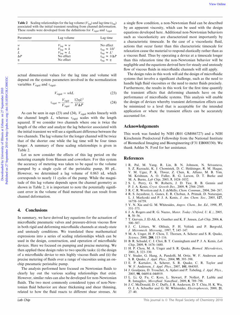
Table 2 Scaling relationships for the lag volume (Vlag) and lag time (tlag)associated with the initial transient resulting from channel deformation.These results were developed from the definitions for Vrigid and srigid

Parameter Lag volume Lag time

w Vlag z w No effecth Vlag z h tlag z 1/h2

L Vlag z L tlag z L2

DP No effect tlag z 1/DPh No effect tlag z h

Dow

nloa

ded

by U

nive

rsity

of

Illin

ois

at U

rban

a o

n 27

Sep

tem

ber

2010

Publ

ishe

d on

27

Sept

embe

r 20

10 o

n ht

tp://

pubs

.rsc

.org

| do

i:10.

1039

/C0L

C00

035C

View Online

actual dimensional values for the lag time and volume will

depend on the system parameters involved in the normalization

variables Vrigid and srigid.

Vrigid ¼ whL (23)

srigid ¼Vrigid

_V rigid

¼ 12hL2

h2DP(24)

As can be seen in eqn (23) and (24), Vrigid scales linearly with

the channel length L, whereas srigid scales with the length

squared. If we consider two channels where one is twice the

length of the other and analyze the lag behavior associated with

the initial transient we will see a significant difference between the

two channels. The lag volume for the longer channel will be twice

that of the shorter one while the lag time will be four times

longer. A summary of these scaling relationships is given in

Table 2.

Let us now consider the effects of this lag period on the

metering example from Hansen and coworkers. For this system

the accuracy of metering was taken to be equal to the volume

pumped by a single cycle of the peristaltic pump, 80 pL.

However, we determined a lag volume of 0.863 nL which

corresponds to nearly 11 cycles of the pump. While the magni-

tude of this lag volume depends upon the channel geometry as

shown in Table 2, it is important to note the potentially signifi-

cant error in the volume of fluid metered that can result from

channel deformation.

4. Conclusions

In summary, we have derived key equations for the actuation of

microfluidic pneumatic valves and pressure-driven viscous flow

in both rigid and deforming microfluidic channels at steady-state

and unsteady conditions. We translated these mathematical

expressions into a series of scaling relationships which can be

used in the design, construction, and operation of microfluidic

devices. Here we focused on pumping and precise metering. We

then applied these design rules to two specific tasks: (i) the design

of a microfluidic device to mix highly viscous fluids and (ii) the

precise metering of fluids over a range of viscosities using an on-

chip pneumatic peristaltic pump.

The analysis performed here focused on Newtonian fluids to

clearly lay out the various scaling relationships that exist.

However, similar rules can also be developed for non-Newtonian

fluids. The two most commonly considered types of non-New-

tonian fluid behavior are shear thickening and shear thinning,

related to how the fluid reacts to different shear stresses. At

Lab Chip

a single flow condition, a non-Newtonian fluid can be described

by an apparent viscosity, which can be used with the design

equations developed here. Additional non-Newtonian behaviors

such as viscoelasticity are characterized most importantly by

a characteristic timescale. In the case of a viscoelastic fluid,

actions that occur faster than this characteristic timescale for

relaxation cause the material to respond elastically rather than as

a viscous fluid. Thus by operating a device at a timescale longer

than this relaxation time the non-Newtonian behavior will be

negligible and the equations derived here for steady and unsteady

flow of viscous fluids in microfluidic channels will still apply.

The design rules in this work will aid the design of microfluidic

systems that involve a significant challenge, such as the need to

handle high fluid viscosities or the need to meter fluids precisely.

Furthermore, the results in this work for the first time quantify

the transient effects that deforming channels have on the

performance of microfluidic systems. This analysis will enable

the design of devices whereby transient deformation effects can

be minimized to a level that is acceptable for the intended

application or where the transient effects can be accurately

accounted for.

Acknowledgements

This work was funded by NIH (R01 GM086727) and a NIH

Kirschstein Predoctoral Fellowship from the National Institute

of Biomedical Imaging and Bioengineering (F31 EB008330). We

thank Ashlee N. Ford for her assistance.

References

1 R. Pal, M. Yang, R. Lin, B. N. Johnson, N. Srivastava,S. Z. Razzacki, K. J. Chomistek, D. C. Heldsinger, R. M. Haque,V. M. Ugaz, P. K. Thwar, Z. Chen, K. Alfano, M. B. Yim,M. Krishnan, A. O. Fuller, R. G. Larson, D. T. Burke andM. A. Burns, Lab Chip, 2005, 5, 1024–1032.

2 S. L. Perry, G. W. Roberts, J. D. Tice, R. B. Gennis andP. J. A. Kenis, Cryst. Growth Des., 2009, 9, 2566–2569.

3 R. C. R. Wootton and A. J. deMello, Chem. Commun., 2004, 266–267.4 R. S. Jayashree, L. Gancs, E. R. Choban, A. Primak, D. Natarajan,

L. J. Markoski and P. J. A. Kenis, J. Am. Chem. Soc., 2005, 127,16758–16759.

5 Y. N. Xia and G. M. Whitesides, Angew. Chem., Int. Ed., 1998, 37,551–575.

6 J. A. Rogers and R. G. Nuzzo, Mater. Today (Oxford, U. K.), 2005,8, 50–56.

7 T. Gervais, J. El-Ali, A. Gunther and K. F. Jensen, Lab Chip, 2006, 6,500–507.

8 J. C. L€otters, W. Olthuis, P. H. Veltink and P. Bergveld,J. Micromech. Microeng., 1997, 7, 145–147.

9 M. A. Unger, H. P. Chou, T. Thorsen, A. Scherer and S. R. Quake,Science, 2000, 288, 113–116.

10 B. R. Schudel, C. J. Choi, B. T. Cunningham and P. J. A. Kenis, LabChip, 2009, 9, 1676–1680.

11 H. P. Chou, M. A. Unger and S. R. Quake, Biomed. Microdevices,2001, 3, 323–330.

12 V. Studer, G. Hang, A. Pandolfi, M. Ortiz, W. F. Anderson andS. R. Quake, J. Appl. Phys., 2004, 95, 393–398.

13 E. P. Kartalov, A. Scherer, S. R. Quake, C. R. Taylor andW. F. Anderson, J. Appl. Phys., 2007, 101, 064505.

14 J. Goulpeau, D. Trouchet, A. Ajdari and P. Tabeling, J. Appl. Phys.,2005, 98, 044914–044919.

15 L. Li, Q. Fu, C. Kors, L. Stewart, P. Nollert, P. Laible andR. Ismagilov, Microfluid. Nanofluid., 2009, 8, 789–798.

16 J. C. McDonald, D. C. Duffy, J. R. Anderson, D. T. Chiu, H. K. Wu,O. J. A. Schueller and G. M. Whitesides, Electrophoresis, 2000, 21,27–40.



Dow

nloa

ded

by U

nive

rsity

of

Illin

ois

at U

rban

a o

n 27

Sep

tem

ber

2010

Publ

ishe

d on

27

Sept

embe

r 20

10 o

n ht

tp://

pubs

.rsc

.org

| do

i:10.

1039

/C0L

C00

035C

View Online

17 M. E. Vlachopoulou, A. Tserepi, P. Pavli, P. Argitis, M. Sanopoulouand K. Misiakos, J. Micromech. Microeng., 2009, 19, 015007.

18 R. B. Bird, W. E. Stewart and E. N. Lightfoot, Transport Phenomena,John Wiley & Sons, New York, 1960.

19 B. S. Hardy, K. Uechi, J. Zhen and H. P. Kavehpour, Lab Chip, 2009,9, 935–938.

20 M. A. Holden, S. Kumar, A. Beskok and P. S. Cremer, J. Micromech.Microeng., 2003, 13, 412–418.

21 S. Timoshenko, Strength of Materials, Part II: Advanced Theory andProblems, D. Van Nostrand Company, Inc., Princeton, NJ, 1955.

22 A. E. H. Love, A Treatise on the Mathematical Theory of Elasticity,Cambridge University Press, Cambridge, 1934.


23 MATLAB version 7.6.0.234, Mathworks Inc., Natick, MA,2008.

24 C. L. Hansen, M. O. A. Sommer and S. R. Quake, Proc. Natl. Acad.Sci. U. S. A., 2004, 101, 14431–14436.

25 T. M. Squires and S. R. Quake, Rev. Mod. Phys., 2005, 77, 977–1026.26 A. D. Stroock, S. K. W. Dertinger, A. Ajdari, I. Mezic, H. A. Stone

and G. M. Whitesides, Science, 2002, 295, 647–651.27 A. D. Stroock, S. K. Dertinger, G. M. Whitesides and A. Ajdari, Anal.

Chem., 2002, 74, 5306–5312.28 J. M. Ottino, The kinematics of mixing: stretching, chaos, and

transport, Cambridge University Press, Cambridge, 1989.29 M. Caffrey, Annu. Rev. Biophys., 2009, 38, 29–51.

Lab Chip


design rules for pumping and metering of highly viscous...

Documents