design structure matrix : models, applications and data …

DESIGN STRUCTURE MATRIX : MODELS, APPLICATIONS AND DATAEXCHANGE FORMAT

RUMANA QUASHEMBachelor of Science, North South University, 2013

A ThesisSubmitted to the School of Graduate Studies

of the University of Lethbridgein Partial Fulfillment of the

Requirements for the Degree

MASTER OF SCIENCE

Department of Mathematics and Computer ScienceUniversity of Lethbridge

LETHBRIDGE, ALBERTA, CANADA

c© Rumana Quashem , 2015

DESIGN STRUCTURE MATRIX : MODELS, APPLICATIONS AND DATAEXCHANGE FORMAT

RUMANA QUASHEM

Date of Defense: October 9, 2015

Dr. Shahadat HossainSupervisor Associate Professor Ph.D.

Dr. Daya GaurCommittee Member Professor Ph.D.

Dr. Robert BenkocziCommittee Member Associate Professor Ph.D.

Dr. Howard ChengChair, Thesis Examination Com-mittee

Associate Professor Ph.D.

Dedication

To

My Loving Parents

iii

Abstract

The Design Structure Matrix model has facilitated the study of design structure and ar-

chitectural complexity of complex systems by analyzing dependencies between system’s

elements. There exists examples and applications of different DSM types highlighting real

world engineered systems in the literature provided by the researchers and authors. Un-

fortunately, there does not exist any specialized digital format that can make those DSM

examples data accessible to public for further analysis. Having said this, in this thesis, we

propose a Data Exchange file format suitable for Design Structure Matrix (DSM) models.

The DSM Data Exchange (DSMDE) file format can be considered as a common file for-

mat that supports DSM data to be exchanged in an organized manner. Thus, we (more)

formally propose an extension to an existing “appropriate” exchange file format instead of

creating a new one. We choose “Matrix Market (MM) file format” for extension to store

DSM information. As DSM techniques are playing a vital role to model and analyze com-

plex network in the area of product development, we believe that our DSMDE file format

will contribute to establish a common standard of exchanging DSM data to the researchers

and developers.

iv

Acknowledgments

I acknowledge with great appreciation the valuable role and encouragement of a number of

people.

I would like to acknowledge my indebtedness to my supervisor Dr. Shahadat Hossain for

his kind attention giving moral support for the selection of topic. I am thankful to him for

giving me the opportunity to work on such a challenging and interesting project and for

providing me various important suggestions. Without his constant guidance, keen interest

and encouragement this thesis would not have been completed successfully.

I would like to thank my co-supervisor Dr. Robert Benkoczi and Dr. Daya Gaur for their

kind support and cooperation.

I pay my immense gratitude to my parents and siblings for their unlimited prayers and for

encouraging me for the completion of my research.

I would like to thank my friends Soma Farin Khan, Marzia Sultana, Mahmudun Nabi and

S M Erfanul Kabir for their constant thoughtful contribution.

Thank you.

v

Contents

Contents vi

List of Tables viii

List of Figures ix

1 Introduction 11.1 Study of complex software architecture . . . . . . . . . . . . . . . . . . . 11.2 Scientific software . . . . . . . . . . . . . . . . . . . . . . . . . . . . . . 21.3 Complex networks . . . . . . . . . . . . . . . . . . . . . . . . . . . . . . 21.4 Design Structure Matrix . . . . . . . . . . . . . . . . . . . . . . . . . . . 31.5 Contribution of the thesis . . . . . . . . . . . . . . . . . . . . . . . . . . . 3

2 The Design Structure Matrix 52.1 What is DSM? . . . . . . . . . . . . . . . . . . . . . . . . . . . . . . . . . 52.2 Brief history of DSM . . . . . . . . . . . . . . . . . . . . . . . . . . . . . 62.3 System architecture and DSM . . . . . . . . . . . . . . . . . . . . . . . . 82.4 Classification of DSM models . . . . . . . . . . . . . . . . . . . . . . . . 92.5 Existing DSM analysis techniques . . . . . . . . . . . . . . . . . . . . . . 182.6 Brief introduction to Domain Mapping Matrix(DMM) . . . . . . . . . . . . 21

3 Dependency analysis using Understand tool 233.1 Code analysis tools . . . . . . . . . . . . . . . . . . . . . . . . . . . . . . 23

3.1.1 Importance of code analysis tools . . . . . . . . . . . . . . . . . . 233.1.2 Types of code analysis . . . . . . . . . . . . . . . . . . . . . . . . 233.1.3 Unit of analysis . . . . . . . . . . . . . . . . . . . . . . . . . . . . 243.1.4 Introduction to “Understand” . . . . . . . . . . . . . . . . . . . . . 243.1.5 Specifics of the tool . . . . . . . . . . . . . . . . . . . . . . . . . . 243.1.6 Projects analyzed . . . . . . . . . . . . . . . . . . . . . . . . . . . 253.1.7 Six types of dependencies . . . . . . . . . . . . . . . . . . . . . . 253.1.8 Overall dependency graph of scanner . . . . . . . . . . . . . . . . 30

3.2 Generation of DSMs for the three scientific software . . . . . . . . . . . . 313.3 Evaluation of “Understand” based on analysis . . . . . . . . . . . . . . . . 31

3.3.1 Strength and weakness of the tool . . . . . . . . . . . . . . . . . . 33

4 A data exchange format for Design Structure Models 354.1 Design philosophy . . . . . . . . . . . . . . . . . . . . . . . . . . . . . . 354.2 Matrix Market Exchange file format . . . . . . . . . . . . . . . . . . . . . 37

4.2.1 Structure of Matrix Market Exchange file format . . . . . . . . . . 37

vi

CONTENTS

4.3 The extended file format for DSM and MDM data . . . . . . . . . . . . . . 414.4 DSMDE grammar . . . . . . . . . . . . . . . . . . . . . . . . . . . . . . . 48

4.4.1 EBNF grammar for DSMDE exchange file format . . . . . . . . . 504.4.2 DSM models in DSMDE file format . . . . . . . . . . . . . . . . . 50

5 Conclusion 65

Bibliography 67

vii

List of Tables

4.1 Header field and their values in DSMDE . . . . . . . . . . . . . . . . . . . 45

viii

List of Figures

2.1 A static call graph [31] . . . . . . . . . . . . . . . . . . . . . . . . . . . 72.2 Corresponding DSM for the call graph [31] . . . . . . . . . . . . . . . . 72.3 Hierarchy of DSMs [12] . . . . . . . . . . . . . . . . . . . . . . . . . . . 92.4 Quantification scheme [24] . . . . . . . . . . . . . . . . . . . . . . . . . 112.5 Component-based original DSM of automobile climate control system

[24] . . . . . . . . . . . . . . . . . . . . . . . . . . . . . . . . . . . . . . 112.6 Clustered DSM [24] . . . . . . . . . . . . . . . . . . . . . . . . . . . . . 122.7 Team-based original DSM of product development teams [14] . . . . . 132.8 DSM after clustering [14] . . . . . . . . . . . . . . . . . . . . . . . . . . 142.9 Activity-based original DSM of automobile design process [20] . . . . . 162.10 Resequenced DSM [20] . . . . . . . . . . . . . . . . . . . . . . . . . . . 162.11 Parameter-based original DSM of robot arm design [25] . . . . . . . . . 172.12 Resequenced DSM [25] . . . . . . . . . . . . . . . . . . . . . . . . . . . 172.13 Classical DSM techniques for types of DSMs [9] . . . . . . . . . . . . . 182.14 DSM after partitioning [30] . . . . . . . . . . . . . . . . . . . . . . . . . 192.15 Original DSM and partitioned DSM of a brake example [30] . . . . . . 202.16 Original DSM [21] . . . . . . . . . . . . . . . . . . . . . . . . . . . . . . 202.17 Clustered DSM [21] . . . . . . . . . . . . . . . . . . . . . . . . . . . . . 212.18 DSM and DMM modeling framework [9] . . . . . . . . . . . . . . . . . 22

3.1 File dependency graph of Scanner . . . . . . . . . . . . . . . . . . . . . 263.2 Call dependency of Scanner . . . . . . . . . . . . . . . . . . . . . . . . . 263.3 init() calls insert() . . . . . . . . . . . . . . . . . . . . . . . . . . . . . . 273.4 Call dependency of init() . . . . . . . . . . . . . . . . . . . . . . . . . . 273.5 Scanner sets three objects . . . . . . . . . . . . . . . . . . . . . . . . . . 273.6 Set dependency of Scanner . . . . . . . . . . . . . . . . . . . . . . . . . 283.7 ’Symtable’ modifies its object ’numEntries’ . . . . . . . . . . . . . . . . 283.8 Modify dependency of Scanner . . . . . . . . . . . . . . . . . . . . . . . 283.9 Scanner uses three objects . . . . . . . . . . . . . . . . . . . . . . . . . 293.10 Uses dependency of Scanner . . . . . . . . . . . . . . . . . . . . . . . . 293.11 Token inits object . . . . . . . . . . . . . . . . . . . . . . . . . . . . . . 293.12 Inits dependency of Scanner . . . . . . . . . . . . . . . . . . . . . . . . 303.13 Overall dependency of class Scanner . . . . . . . . . . . . . . . . . . . . 30

4.1 Header combinations of MM matrices [11] . . . . . . . . . . . . . . . . 394.2 Qualifier: field [11] . . . . . . . . . . . . . . . . . . . . . . . . . . . . . 404.3 Qualifier: symmetry [11] . . . . . . . . . . . . . . . . . . . . . . . . . . 40

ix

Chapter 1

Introduction

The complexity of today’s product design structure is determined by its architecture where

there exists complex interactions between design components. The Design Structure Ma-

trix modeling technique is known as a special tool to model these design complexities

based on interactions. Many real world examples of DSM matrices remain scattered in the

literature. These practical DSM examples from different application areas establish an im-

portant database of scientific knowledge. But most of these examples can not be retrieved

easily in a digital form. Therefore, there is a need of having a standardized file format

that makes DSM data publicly available. Our aim is to identify “suitable” existing data

exchange format and extend it to incorporate DSM data.

1.1 Study of Complex Software Architecture

The complexity in a software architecture is established by its components and their in-

teraction [27]. Certain techniques are needed for mastering these large amount of system’s

activities and their interconnections which also includes understanding, designing and im-

proving systems. For example, an advanced complex software architecture requires a de-

sign architecture that is easily accessible to any changes in functions and re-development

of any parts of the system [18]. From an engineering perspective, a modularized design of

a product makes complexity manageable, enables parallel work and accommodates future

uncertainty. The elements of modular product design can be easily divided and assigned to

different modules representing the interdependence within modules and independence be-

tween modules. In 2000, the authors Baldwin and Clark [22] have incorporated two ideas

about modularity: the need for carrying out a specific work on the given module with-

1

1.3. COMPLEX NETWORK

out causing any changes to other modules in the design, and the need for well-designed

interfaces between these modules.

1.2 Scientific Software

Computer software can be viewed as a network of interacting modules. Poor software

designs are designs that are hard to modify and reuse. Improper dependencies of software

modules are another main cause of a poorly structured design. Changes are made when

the initial design can not predict certain requirements of overall design of the product. As

a result, design degrades and those changes introduce new and unplanned dependencies

between the modules of the system. Scientific software are made up of large numbers

of modules that are being developed to perform large-scale simulation run [7]. They are

designed and developed in such a way that any part of it can be modified if changes in

requirements are made [19, 23]. Thus, the major properties we expect to be displayed by

general software and scientific software in particular, are reusability, extendibility, correct-

ness, verifiability, robustness, efficiency and portability.

In this thesis, we discuss the DSM modeling as it applies to the product, process and or-

ganization design architecture. Furthermore, we evaluate tool to extract dependency in-

formation/data from scientific software code and generate their DSMs. We propose a data

exchange format to facilitate the exchange of dependency data.

1.3 Complex Networks

The term network implies different interpretations in different areas. In the social sci-

ences, the term ’network’ is formally studied as ’graphs’. Graphs are referred to a set of

nodes or vertices which may have links or edges with one another. The most common form

of matrix in social network analysis is a ’square matrix’ with rows and columns. The cells

of the matrix record information about each pair of nodes such as their weights. That is, if

the value of the cell is 1, it represents the presence of an edge; otherwise, it is 0. This kind

2

1.5. CONTRIBUTION OF THE THESIS

of matrix is called ’adjacency matrix’. It is a powerful tool to conduct several analyses of

graphs [17]. In our thesis, the study of dependency structure of design structure matrix

(DSM) model can be viewed as complex network.

1.4 Design Structure Matrix

The DSM is a network modeling tool that highlights the inherent structure of a de-

sign. A DSM model displays the dependencies that exist between system components and

highlights the types and sources of such dependencies concisely. Many alternative terms

have been applied such as Dependency Structure Matrix, Dependency System Model, and

Deliverable Source Map to emphasize particular aspects of DSM models [15]. This model

provides some advantages for system architecture modeling such as conciseness (represent-

ing fairly large and complex systems in a relatively small space), visualization (provides a

system level view), intuitive understanding (understanding a basic structure of a complex

system easily), analysis (applies powerful analyses in graph theory and linear algebra), and

flexibility (modification and extension the basic DSM with helpful graphics etc.) [15].

1.5 Contribution of the thesis

A DSM is much more than an adjacency matrix representation of a graph. A project

may involve interactions that are far more complex than simple binary interactions. In

an application described in Eppinger and Browning [15], there are three different sources

of interactions where each interaction can be one of three different types. Thus, different

choices for system elements and interaction categories yield alternative contextual models

for the same modeling exercise.

In Chapters 2 and 3, we have reviewed DSM techniques that are relevant and useful in

analyzing complex software architecture. We have employed the dependency extraction

tool Understand [28] to construct DSM models for three important scientific software ap-

plications: ADOL-C, CPPAD, and CSparse. The resulting DSMs can display dependency

3

1.5. CONTRIBUTION OF THE THESIS

information at different level of granularity: from file-level dependencies to object-use de-

pendencies.

In Chapter 4 we have proposed a new file format for the exchange of DSM data. Currently

there does not exist any standard way to exchange DSM data. The proposed DSMDE ex-

change format fills this void. The DSMDE exchange format is derived from the widely

used Matrix Market (MM) file format. The new format is quite flexible in that both single-

domain and multi-domain (MDM) information can be stored in the same file. For MDM

models, the data are organized in a block triangular configuration where the diagonal blocks

correspond to the DSMs and the off-diagonal blocks represent domain mapping matrices

(DMMs). Thus the DSMDE format can handle complex DSM and MDM models in a

uniform manner.

4

Chapter 2

The Design Structure Matrix

In this chapter, we study the importance of design structure matrix, illustrate different types

of DSMs with corresponding examples and their applications.

2.1 What is DSM?

The Design Structure Matrix (DSM) is a network modeling technique to represent the

components of a system and the relationships among them [15]. A system model can be

considered as a graph where a node represents a system element and an edge represents the

relationship between two elements. In case of directed graph(digraph), an arrow between

two elements shows the impact from one element to another. The DSM emerged as a con-

cise matrix representation of digraphs. The approach has become widespread for analyzing

complex system models. It is a square adjacency matrix containing identical row and col-

umn captions. The diagonal cells depict the components of a system and off-diagonal cells

depict the dependency among these components [15]. In terms of advantages, the DSMs

provide more visual advantages including compactness and clear representation of essen-

tial patterns. On the other hand, as the graph becomes larger with nodes and edges, it gets

more difficult to understand the overall representation of the network.

Several earlier project management tools named PERT (Program Evaluation and Review

Technique) and CPM (Critical Path Method) methods [5] lack managing a common phe-

nomenon of complex product development, that is ’interdependency’ (iterations) [30]. The

DSM tool overcomes this shortfall.

5

2.2. BRIEF HISTORY OF DSM

2.2 Brief History of DSM

The use of matrices and graph theory for modeling large and complex engineering

projects has been found in the work of Warfield and Steward respectively in the 1970s

and 1980s [26]. In 1981, Don Steward first came up with the design structure matrix

as a network representation where he explained how design tasks interact with each other

[9]. Later on, in the 1990s, this method caught the attention of large number of design

developers and became widespread. MIT researchers applied DSM since the 1990s in their

research work on product and system development [4].

In 2012, Eppinger et al. expanded this model to capture more ideas about relationships

between product elements.

“ Engineering work can be procedural and systematic,” says Eppinger. “People think of

engineering as a matter of always developing something new, unlike business operations,

where you do something over and over again. But we’ve learned that while you may repeat

engineering work five or 20 times in your career instead of 100 times a day, there is a

process there. And if you can capture that process, you can improve it.”

Example of a graph and its corresponding DSM:

Consider the graph in Figure 2.1. A static call graph is displayed where functions are

represented as nodes and a directed edge between two nodes represents a function call.

Here, function 1 calls functions 3 and 4. Thus, there is an edge from function 1 to functions

3 and 4. A corresponding DSM is displayed in Figure 2.2. Marks on cells 3 and 4 in row

1 depict element 1 requires information from elements 3 and 4.

If component A requires information (represented by a mark on off-diagonal cell) from

component B, such information depicts the input for component A. On the other hand, if

component A provides information to component B, such information represents the output

for component A.

There are two conventions for reading an element’s inputs and outputs in the DSM [15].

1. IR/FAD: The off-diagonal mark in IR depicts Input in Row and output in column.

6

2.2. BRIEF HISTORY OF DSM

Figure 2.1: A static call graph [31]

Figure 2.2: Corresponding DSM for the call graph [31]

With IR in a process DSM, “feedback” is depicted as a mark above the main diago-

nal(FAD).

2. IC/FBD: The off-diagonal mark in IC depicts Input in Column and output in Row.

With IC in a process DSM, “feedback” is depicted as a mark below the main diago-

nal(FBD).

To indicate the presence or absence of a dependency in the off-diagonal cell, there are two

types of DSMs [15].

1. The binary DSM is represented putting dots or marks in the off-diagonal cell that

shows a direct relationship between two elements.

7

2.4. CLASSIFICATION OF DSM MODELS

2. The numerical DSM consists of numbers, colors, shades or symbols in the off-

diagonal cell to show the dependency intensity and strength between two elements.

2.3 System Architecture and DSM

A system’s architecture describes system components and their interactions as a struc-

ture that can be designed and developed over time [15].

Here we present Eppinger’s [15] modified IEEE definition of system architecture.

Definition 2.1. The structure of a system is embodied in its elements, their relationships

to each other (and to the system’s environment), and the principles guiding its design and

evolution- that gives rise to its functions and behaviors.

Products, processes and organizations can be viewed as complex system architectures.

The design structure matrix (DSM) model gives a concise and simple representation of

system architecture.

Classic DSM Approach to System Architecture Modeling:

In 2012, Eppinger et al. [15] mentioned five step approach to model and analyze each of

the DSM applications. The steps are:

1. Decompose: Breaking a system into several subsystems.

2. Identify: Recording all the interactions among the system’s components.

3. Analyze: Reorganizing the components and their interactions (integration) in order

to get the precise idea of system behavior.

4. Display: Visual graphical representation of the DSM model focusing on important

features.

5. Improve: Actions taken during the analysis of DSM improving the system as a whole.

8


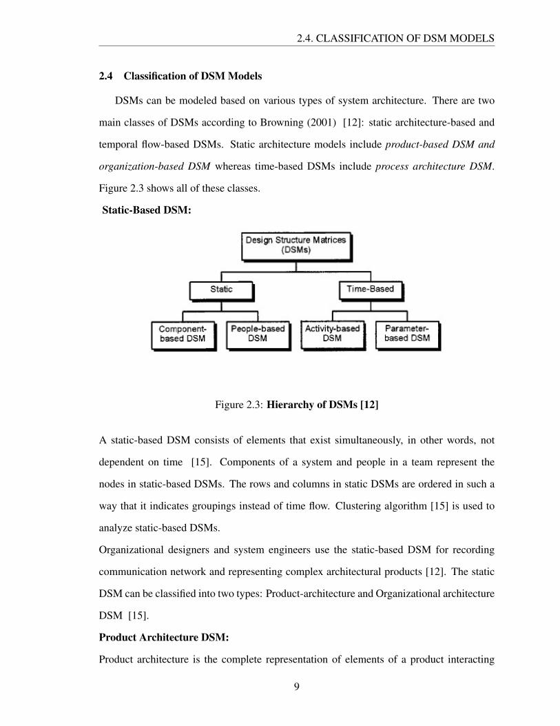
2.4 Classification of DSM Models

DSMs can be modeled based on various types of system architecture. There are two

main classes of DSMs according to Browning (2001) [12]: static architecture-based and

temporal flow-based DSMs. Static architecture models include product-based DSM and

organization-based DSM whereas time-based DSMs include process architecture DSM.

Figure 2.3 shows all of these classes.

Static-Based DSM:

Figure 2.3: Hierarchy of DSMs [12]

A static-based DSM consists of elements that exist simultaneously, in other words, not

dependent on time [15]. Components of a system and people in a team represent the

nodes in static-based DSMs. The rows and columns in static DSMs are ordered in such a

way that it indicates groupings instead of time flow. Clustering algorithm [15] is used to

analyze static-based DSMs.

Organizational designers and system engineers use the static-based DSM for recording

communication network and representing complex architectural products [12]. The static

DSM can be classified into two types: Product-architecture and Organizational architecture

DSM [15].

Product Architecture DSM:

Product architecture is the complete representation of elements of a product interacting

9


to perform specified functions [15]. The product development firms now greatly rely on

product architectures because of its revolutionary features and advantages.

Product architecture DSM is a mapping of the network of interactions among a product’s

components/elements [15]. It is also known as product DSM, system architecture DSM,

Component DSM.

System Engineers follow three major steps for every complex system development project

[15]:

1. Decompose the system into elements;

2. Understand and record the interactions between the elements (i.e., their integration);

3. Analyze potential reintegration of the elements via clustering (integration analysis).

Example 2.2. Pimmler and Eppinger [15] used component-based DSMs to exhibit alter-

native architectures at Ford Motor Company [12]. Their goal was to improve the quality

of the resulting product design at Ford Motor Company. Figures 2.5 and 2.6 show the

materials-type interaction for an automotive climate control system, where numeric value

quantifies the importance/strength of that specific interaction type. In Figure 2.6, three

groups/modules/clusters have been identified considering only the materials-type interac-

tions. Components within a cluster have many strong interactions (intra-group interac-

tions). Components among three clusters have relatively few interactions (inter-group in-

teractions). For instance, there exists strong interactions among components of front-end

air cluster while there exists few interactions between components of cluster front-end air

and cluster refrigerant.

In 2012, Eppinger et al. [9] provided more component-based DSM examples in their book

that include building construction, semiconductor, photographic, aerospace, electronics,

and telecom industries.

Organizational Architecture DSM:

10


Figure 2.4: Quantification scheme [24]

Figure 2.5: Component-based original DSM of automobile climate control system [24]

Organization is one of the most complex systems. Communication among different group-

s/teams within the organization is the crucial part of complex organizational system de-

velopment. Organization DSMs analyze an organization, captures the structure of organi-

zational units and designs it according to the communication flow among organizational

units such as individuals, teams, groups, departments etc. It specially focuses on informa-

tion flow interactions [15]. The individual group/team member or groups/teams within the

organization are considered to be the nodes (the diagonal cells of the DSM) and the com-

munication flow between nodes represent interactions (the off-diagonal cells) [9]. This

DSM is also known as organization DSM, people-based DSM, team-based DSM.

To build an organizational DSM as system model, it requires the following three steps [15]:

11


Figure 2.6: Clustered DSM [24]

1. Decompose the organization into elements (e.g., teams) with specific functions, roles,

or assignments;

2. Record the interactions between (the integration of) the teams;

3. Apply clustering analysis(assigning organizational units to teams). Interactions be-

tween clusters or metateams are to be minimized [12].

Example 2.3. McCord and Eppinger [15] applied the team-based DSM to analyze an

automobile engine (General Motors) development project. They encapsulated the com-

munication frequency between the component development teams (CDTs) (Figure 2.7).

Figure 2.7 shows the DSM that decomposes the organization into 22 CDTs and records the

frequency (daily, weekly, monthly) of communications between the teams.

In the next step, the DSM is restructured through clustering analysis by assigning CDTs

into more groups/subsystem teams based on the reported frequency of their interactions as

shown in the Figure 2.8. The resultant DSM consists of five groups. First four groups/-

subsystem teams represent a formal organization structure of higher level groupings [15].

Two component development teams B and K are shown twice since they are assigned to

12


two or three subsystem teams; each participating in three subsystem teams.

The five CDTs H, S, T, U and V at the bottom of the matrix do not fit systematically into

the four subsystem teams since they need to merge with all of the four subsystem teams.

Therefore, these five CDTs form another integration team. For instance, one representa-

tive from each CDT of this integration team will attend each of the four subsystem team

meetings [12].

Figure 2.7: Team-based original DSM of product development teams [14]

Several other researchers Browning and Danilovic [9] applied organizational DSM to the

aerospace and automotive industries.

Temporal-Flow DSM:

Unlike static DSMs, the nodes in temporal flow DSMs are time dependent [15]. Thus, the

ordering of rows and columns in such DSMs depict time sequence or activity flow through

time [9]. Time-based DSM includes architecture of processes; represented as activity/task

based process models and low-level parameter based models [15].

13


Figure 2.8: DSM after clustering [14]

The time-based DSM is analyzed using partitioning process (will be discussed later in this

chapter). The feedback marks are reduced or eliminated using this process [30]. Once

the partitioning process is done, three types of activities are identified in the restructured

process DSM. These activities include-

• Sequential: One element influences the behavior of another element. For example,

project task A has to be performed first before task B can start.

• Parallel: System elements do not interact with each other. For example, task A is

independent of task B. There is no information exchange between two tasks.

• Coupled: The flow of information is interdependent. For example, design parameter

A can not be determined without first knowing parameter B and B could not be

determined without knowing A.

14


Activity-based DSM:

A process refers to a project/system that is comprised of a set of activities/tasks and their

interactions (input-output relationships). To represent such system, we can use the matrix

approach with the DSM methodology. These DSMs are called process architecture DSMs.

It is a mapping of the network of interactions among tasks/activities in a process [15].

Such DSMs are also known as task-based DSM, process DSM. They are used to depict

the dependency of one activity on another, more precisely, to identify activities that are

required to be finished first for other activities to start [9]. The rows and columns of

such DSMs are the lists of tasks/activities to be performed. Information based interactions

among tasks/activities are represented as marks in the matrix. Marks below the diagonal

are known as forward marks that transfers forward information to later tasks. Marks above

the diagonal are known as feedback marks that feeds back information to earlier tasks [30].

Three steps are required to model process DSM [15]:

1. Decompose the process into activities;

2. Document the information flow among the activities (their integration);

3. Analyze the sequencing of the activities.

Example 2.4. In 1993, Kusiak and Wang [9] applied an activity-based DSM to a simple

automobile design process. In this example, the design tasks represent the nodes of the

system; the interaction (information flow/input-output) between activities are represented

as relations in the system (Figure 2.9). In the Figure 2.9, the DSM contains 11 feedback

marks. Figure 2.10 displays the resequenced DSM after implementing a block diagonal-

ization algorithm [15]. In the resequenced DSM (Figure 2.10), feedback marks are reduced

to 5 and two coupled tasks are identified.

Parameter-based DSM:

A parameter-based DSM is constructed from a ”bottom-up” approach to identify the low

15


Figure 2.9: Activity-based original DSM of automobile design process [20]

Figure 2.10: Resequenced DSM [20]

level parameters that determine the design. The nodes of such DSMs represent system

activities which may include tasks describing how the physical system works. While an

activity-based DSM might include tests, reviews etc. within the system, a parameter-based

DSM determines tasks that highlight the physical relationships between parameters [9].

The methods used for modeling a parameter-based DSM are very identical to the methods

used in an activity-based DSM. Parameter based DSMs are the least documented in the

16


literature.

Example 2.5. Rask and Sunnersjo [25] in 1998 applied a parameter-based DSM to demon-

strate the relationships between design variables of a robot arm and its housing (Figure

2.11). In the Figure 2.11, two system components“robotic housing” and “robotic arm” are

Figure 2.11: Parameter-based original DSM of robot arm design [25]

Figure 2.12: Resequenced DSM [25]

17

2.5. EXISTING DSM ANALYSIS TECHNIQUES

decomposed into their design parameters and have been isolated into two coupled activi-

ties [9]. In the second Figure 2.12, sequencing is applied and two coupled activities have

been combined into one single activity. The restructured DSM allowed all of the low level

parameters to be determined sequentially [12].

2.5 Existing DSM Analysis Techniques

The following table in Figure 2.13 displays classical DSM techniques for all types of

DSMs.

Partitioning / Sequencing:

Figure 2.13: Classical DSM techniques for types of DSMs [9]

Compared to graphs, it is much easier to find out and analyze feedback relationships in

DSM models [30]. Feedback marks in DSMs correspond to those inputs that are not avail-

able at the time of executing a task. Partitioning/Sequencing is one of the most common

methods of analysis in time-based DSM models that deals with feedback marks in the DSM

matrices. With IR convention, feedback marks exist above the main diagonal. With IC con-

vention, feedback marks exist below the main diagonal.

Partitioning is the procedure of reordering DSM rows and columns to reduce/eliminate

feedback marks; thus altering the DSM into a block diagonal/lower triangular form [9].

Three tasks can be identified after sequencing.

18


Example 2.6. In the example DSM in Figure 2.14, B feeds C, F, G, J and K and D is fed by

E, F and L [30]. All marks above the diagonal are feedback marks. Applying sequencing

in the original DSM, the feedback marks are reduced to 4 and three tasks are identified.

Figure 2.14: DSM after partitioning [30]

Application:

The following Figure 2.15 is an example application of parameter based DSM before se-

quencing and after sequencing.

Clustering:

Clustering analysis is a useful procedure for analyzing component-based and organization-

based DSMs. Clustering is the process of reordering DSM rows and columns to group

components into a different set of modules/clusters in order to perform specific functions

[15]. The most notable objective of applying clustering into DSMs is to maximize inter-

actions between elements within clusters (modules) and to minimize interactions between

19


Figure 2.15: Original DSM and partitioned DSM of a brake example [30]

clusters [9].

Figure 2.16: Original DSM [21]

20

2.6. BRIEF INTRODUCTION TO DOMAIN MAPPING MATRIX(DMM)

Figure 2.17: Clustered DSM [21]

Example 2.7. In Figure 2.17, the original DSM has been clustered into two groups. It

indicates that interactions among the teams within cluster are most frequent and essential.

Application:

A DSM application (before and after clustering) has been shown in Figures 2.5 and 2.6.

In a development process, if it is required to make several development teams within the

project, clustering can be used to make teams and assign members in each team [21].

2.6 Brief Introduction to Domain Mapping Matrix(DMM)

A DSM represents single-domain interaction patterns. To analyze multidomain interac-

tions, Domain Mapping Matrix(DMM) technique is used. It defines a mapping two or more

domains at once. The rows in DMM represent elements of one domain and the columns

represent elements of another domain. Thus a DMM is an mxn rectangular matrix whereas,

a DSM contains identical rows and columns.

Eppinger [9] and several other researchers recognized that the analysis of single-domain

21

2.6. BRIEF INTRODUCTION TO DOMAIN MAPPING MATRIX(DMM)

interaction pattern guides to study about a particular product and its improvement, while

the analysis of multi-domain interaction pattern allows assessment of “effectiveness of the

process and organization to develop the particular product.”

Example 2.8. In 2007, Danilovic and Browning [9] modeled an MDM framework (Figure

2.18).

In the Figure 2.18, An MDM model has been displayed. This is an MDM model com-

Figure 2.18: DSM and DMM modeling framework [9]

prised of five DSMs and their corresponding DMMs. An MDM model can be viewed as

lower/upper triangular matrix. The diagonal blocks of the model correspond to DSMs in-

teracting within each of the five domains and the off-diagonal blocks correspond to DMMs

that define a mapping between domains [9].

22

Chapter 3

Dependency Analysis Using Understand Tool

In this chapter, the use of an existing tool to create/extract static dependency graph/data is

elaborated. It also provides a discussion on the procedure to construct DSMs from depen-

dency data generated by the tool.

3.1 Code Analysis Tools

In this section, we briefly describe the notion of code analysis, importance of certain

code analysis tools and the tool we used for our work.

3.1.1 Importance of Code Analysis Tools

Code analysis is a significant process to achieve clear understanding of the source code.

An effective code analysis tool can provide more accuracy in source code analysis of soft-

ware. Using the tool, we can measure the quality of a software by the code metrics it

provides [8]. Code metrics are a set of software measures such as: number of lines, num-

ber of statements, number of functions etc.

3.1.2 Types of Code Analysis

There are typically two kinds of code analysis: static analysis and dynamic analysis

[8]. The static code analysis provides code metrics for all programs in a project without

executing the code. Some of the metrics include the number of lines of code, file volume

(the number of files in the program, i.e. code files and header files) etc. On the other hand,

the dynamic code analysis computes the metrics while executing the program. In this thesis,

we focus on the static code analysis for large software projects in C/C++ programming

23

3.1. CODE ANALYSIS TOOLS

languages.

3.1.3 Unit of Analysis

In our work, we mainly examine the source code dependencies based on “function

calls”. However, as we discuss in the later point of the thesis, our analysis can be gen-

eralized to different level of granularity. For our work, we have used a commercial code

analysis tool “Understand version 3.1”. It has many features that will be described in later

sections.

3.1.4 Introduction to “Understand”

The tool Understand focuses on source code comprehension and metrics. It provides

the ability to browse any information about files, classes, methods and “entities” (variables,

functions, files, etc) of software projects. Using the dependency browser of Understand,

we can find out the dependencies between different entities of the project. An entity de-

pends on another one if it includes, calls, uses, sets, modifies or refers to that item. For

example, file A depends on file B if a function of file A calls a function of file B. An in-

formation browser provides any information about the entities of the source code such as

files, classes, members, functions, return type and parameters. The dependencies between

files, classes etc. can be displayed graphically.

3.1.5 Specifics of the tool

Understand provides many features such as: it can be used for different operating sys-

tems [8]; it supports source codes of 17 programming languages C, C++, C#, Objective

C/Objective C++, Ada, Java, Pascal/Delphi, COBOL, JOVIAL, VHDL, Fortran, PL/M,

Python, PHP, HTML, CSS, JavaScript, and XML; it calculates more than 50 metrics for

function, class, file, and project level and provides over 20 different graphs [8]; it generates

the dependencies of large source code and outputs a variety of reports.

24


3.1.6 Projects Analyzed

The projects we analyzed in Understand are as follows: one small-sized project, one

mid-sized project and two large projects.

Small-sized project:

Scanner: We took a small project Scanner to check the tool’s behavior in a boundary case.

The project contained 563 lines of code.

Then we analyzed the following three scientific software libraries. Two of them are large-

sized and one is mid-sized.

Mid-sized Project:

CSparse: CSparse is a scientific software library that implements a number of direct meth-

ods for sparse linear systems, by Timothy Davis [3]. It contains 2383 lines of code.

Large Projects:

1. Adol-C: Adol-C (Automatic Differentiation by Overloading in C++) is an open source

package that facilitates the evaluation of first and higher derivatives of vector func-

tions that are defined by computer programs written in C or C++ [16]. It is developed

by a team of researchers from Argonne National Lab, Dresden University of Tech-

nology,and Humboldt University over a period of 20+ years [29]. It contains 15,804

lines of code.

2. CppAD: CppAD (C plus plus Algorithmic Differentiation) is another Automatic dif-

ferentiation software that generates an algorithm computing corresponding derivative

values [10]. It is developed as a one-person effort at the University of Washington,

Seattle [31]. It contains 23269 lines of code.

3.1.7 Six Types of Dependencies

In this section, we discuss about our dependency analysis of the small project scanner

using Understand.

Class scanner depends on six files (Figure: 3.1): token.h, token.cc, symbol.h, symtable.h,

25


Figure 3.1: File dependency graph of Scanner

symtable.cc, scanner.h.

It contains seven functions: init(), processComment(), recognizeDigit(), recognizeWordsym-

bol(), recognizeSpecialsymbol(), nextToken() and constructor function Scanner().

Includes dependency:

Figure 3.2: Call dependency of Scanner

Class scanner includes scanner.h, token.h, symbol.h, symtable.h at scanner.cc file.

Call dependency:

Four private member functions of scanner class: isalpha(), iscom(), isws() and isnum() are

called by recognizewordsymbol() and nextToken() at scanner.cc (Figure 3.2).

Call dependency between functions of different classes:

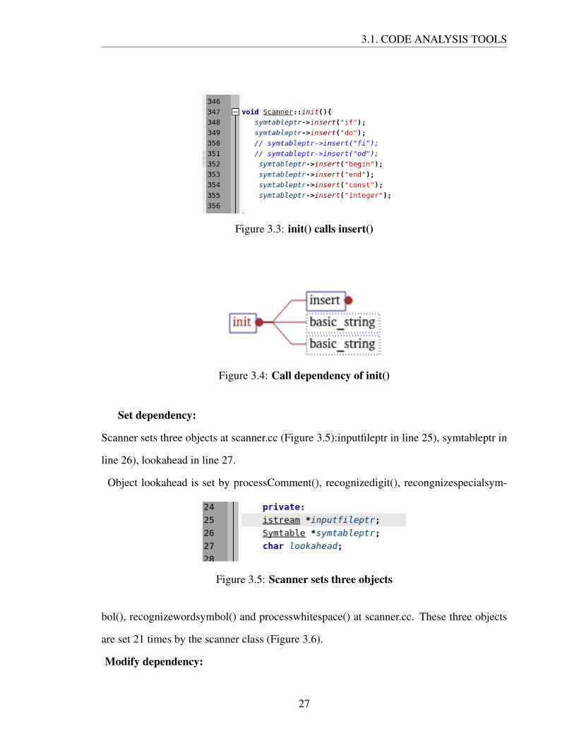
Function init() of class Scanner calls insert() function of class Symtable in line 348 at scan-

ner.cc (Figure 3.4).

26


Figure 3.3: init() calls insert()

Figure 3.4: Call dependency of init()

Set dependency:

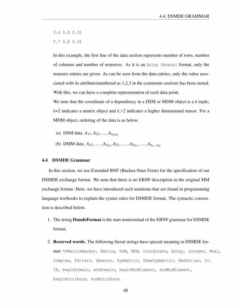
Scanner sets three objects at scanner.cc (Figure 3.5):inputfileptr in line 25), symtableptr in

line 26), lookahead in line 27.

Object lookahead is set by processComment(), recognizedigit(), recongnizespecialsym-

Figure 3.5: Scanner sets three objects

bol(), recognizewordsymbol() and processwhitespace() at scanner.cc. These three objects

are set 21 times by the scanner class (Figure 3.6).

Modify dependency:

27


Figure 3.6: Set dependency of Scanner

The insert() function of Sub-class ’Symtable’ modifies its object ’numEntries’ by incre-

menting its value at symtable.cc in line 124 (Figure:3.7). Class Symtable modifies its

object 2 times at Symtable.cc (Figure 3.8).

Figure 3.7: ’Symtable’ modifies its object ’numEntries’

Figure 3.8: Modify dependency of Scanner

28


Uses dependency:

All six functions of Scanner class use three objects lookahead in line 23, inputfileptr in line

24 and symtableptr in line 36 at scanner.cc (Figure 3.9). Class Scanner uses these three

objects 75 times (Figure 3.10).

Figure 3.9: Scanner uses three objects

Figure 3.10: Uses dependency of Scanner

Inits dependency:

Class Token inits its object ’svalue’ in line 9 and 15 (Figure:3.11). File token.cc inits to-

ken.h 2 times (Figure 3.12).

Figure 3.11: Token inits object

29

3.2. GENERATION OF DSMS FOR THE THREE SCIENTIFIC SOFTWARE

Figure 3.12: Inits dependency of Scanner

3.1.8 Overall Dependency Graph of Scanner

While analyzing the overall dependency of scanner (Figure 3.13), we find a red line

between two files, symtable.h and symtable.cc. This red line indicates a cycle, in other

words, these two files depend on each other.

Symtable.cc↔ Symtable.h

symtable.h: symtable.cc includes symtable.h

symtable.h: symtable.h depends on the function of symtable.cc

Figure 3.13: Overall dependency of class Scanner

30

3.3. EVALUATION OF “UNDERSTAND” BASED ON ANALYSIS

3.2 Generation of DSMs for the Three Scientific Software

Using Understand, we extracted all dependency types (call, set, use, modify and init)

between files of ADOL-C, CppAD and CSparse. The main reason of our analysis is to

create the DSMs representing each type of dependency of these three scientific software

libraries. The data generated from the tool is processed to construct the DSMs.

We followed the following procedure to construct the DSMs.

1. Exporting dependency metrics to CSV file option of Understand tool lists pairs of

files for which the file in column A is dependent upon the file in column B. Column

C lists the number of dependencies for each pair.

2. To extract call dependencies between functions, we went through each file from the

dependency browser.

3. We indexed all functions that were responsible for the dependency between files.

4. We then created a single CSV file that lists pairs of functions for which the function

(of one file) in column A is dependent upon the function (of another file) in column

B. The number of dependencies for each pair is listed in column C.

5. Finally, we wrote a program that read data from our processed CSV file and generated

an output text file representing the DSM.

3.3 Evaluation of “Understand” Based on Analysis

We evaluate Understand both quantitatively, by measuring some of its characteristics,

and qualitatively, by discussing the code analysis features that the tool provides.

Quantitative Evaluation:

1. Number of Dependencies: We took a small project “Scanner” (as discussed earlier)

to check the correctness of the dependencies the tool generated. We followed the

following process.

31


• We computed function call dependencies of “Scanner” by hand.

• Then we used the tool to generate dependencies.

• Finally, we compared the result of hand-computed dependencies against that of

the tool-generated dependencies.

The tool correctly identified call dependencies for “Scanner”. We followed this pro-

cess only for this small project. We did not perform this process for mid-sized and

large-sized projects : ADOL-C, CppAD and CSparse due to limited time.

2. Metrics: Understand provides a number of important metrics information/statistics

about the entities of a project. The Project Metrics Summary provides metric in-

formation about the entire project. It includes: the total number of classes, files,

functions, lines of source code, comment lines, blank lines.

3. Time: The time Understand took to load a project was less than 20 seconds even for

the large and complex projects.

Qualitative Evaluation: It mentions how the different kind of browsers in understand

tool work to find out all dependencies of software projects.

1. Context Menu : Clicking on any entity at anytime from the information browser

points that entity everywhere in the source code. Right-clicking on a specific entity

provides a list of options that contain all information about the entity.

2. Information Browser : Information about an entity of the project can be learned from

the information browser. Information is shown in a tree which can be expanded. It

includes information such as kind and name of the entity, location or path of the

entity in the source code, relationship tree, references (where it is used), statistics for

this entity and so on.

3. Dependency Browser : The Dependency Browser shows which items/entities are

dependent on others. It has the following options: Dependency kind (depends on and

32


depended on by), group by (files, classes and entities), and dependency types (calls,

uses, modifies, includes, inits, sets etc.)

4. Graphical View : Understand analyzes source and creates a graphical view containing

information about the entities and the relations between entities. The graphical views

consist of two kinds [28]:

Hierarchy views show relations between entities. For example: calls(calls or calls

by) relation.

Structure views show the structure of an entity vertically. For instance: declarations

graph of a file or a package.

5. Search Options : Understand provides some efficient searching features of entities in

the source code. These include the Filter Area, the Entity Locator, and the Find in

Files dialog.

3.3.1 Benefits and Weakness of the Tool

Strength:

One of the important strengths of Understand is the speed. From our analysis, we have

observed that loading and analyzing a project into Understand does not take much time.

Even the larger projects took less than twenty seconds to be loaded into the tool. Another

strength of this tool is its flexibility. This tool can cope up well with the size of the project.

Finally, the different browsers of the tool enables dependencies to be displayed in a very

clear and clean manner, even if the project gets very large and complex.

Weaknesses: While analyzing six types of dependency between functions, we observed

that Understand only provides the graphical view of file dependency rather than the de-

pendencies that exist between functions. Also, it exports CSV file that contains only the

dependency information between two files. For instance, in order to come up with a Call

DSM, we had to go through each file in the information browser to find out each function

call. If it would have provided a graphical view of dependence based on functions and

33


exported CSV files containing functional dependency information, we could have created

our DSMs in less time.

34

Chapter 4

A Data Exchange Format for Design Structure Models

4.1 Design Philosophy

In this chapter, we propose a Design Structure Model Data Exchange (DSMDE) file for-

mat as a common file format to promote reliable and efficient exchange of Design Structure

Model (DSM) data and Multidomain Model (MDM) data. We provide the specification of

our proposed format DSMDE, which is an extension of the Matrix Market (MM) file for-

mat, for exchange of DSM and MDM data. The MM exchange format is a simple but

extensible file format for storing and exchanging sparse and dense matrix data. The data

is stored in an ASCII text file. The MM format enables extensibility by allowing format

specialization in the form of qualifier attributes and structured documentation [11]. The

following properties of a common file format are also desired to be present in our DSMDE

file format-

1. Supports human and machine readable storage format of DSM data.

2. Supplies precise and clear documentation that is useful to the users and researchers.

3. Provides users a scope to extend the base format by adding new properties.

There already exists a number of different file formats for the exchange of graph and matrix

data. Hence, we have decided to identify an existing “suitable” format and extend it to

allocate DSM/MDM data rather than creating a new one. Having said this, like other

formats, the following basic features are expected in our DSMDE file format.

1. Portability: The format should allow the data in the file to be easily transferable

between hardware and operating systems and to be displayed with general purpose

35

4.1. DESIGN PHILOSOPHY

text editors such as NotePad,TextEditor, Emacs etc.

2. Simplicity: By simplicity we mean, the syntactic structure of the format required to

describe the data needs to be simple enough not to hinder with human readability.

3. Extensibility: The format should be designed in such a way that it is flexible enough

to allow adaptation and extension of the base format without requiring too much

effort.

The Harwell-Boeing File Format:

The Harwell-Boeing(HB) sparse matrix collection is one of the earliest efforts to compile

and maintain a standard set of sparse matrix test problems emerging in a wide range of

scientific and engineering fields [13]. The matrix is stored as a sequence of “compressed

columns [2]. The two main characteristics of a HB file format are i) ASCII based file for-

mat and ii) FORTRAN programming language oriented [6]. The excessive dependence on

FORTRAN’s specific input/output constructs of HB file formats makes it more complex

for further extension. [11].

GAMFF (Graph and Matrix File Format):

GAMFF [1] is another ASCII based file format closely similar to HB format. But GAMFF

is more flexible in that it allows additional information specific to graphs and hypergraphs.

Similar to HB format, GAMFF also uses ”compressed column storage (CCS)” to store non-

zero entries.

The complication in extending both the HB and GAMFF format is their nature of using

compressed column (CCS). The problem arises due to the ”integer index overflow” result-

ing from CCS (or compressed row (CRS)) in HB and GAMFF formats. For example, if we

consider a nxn sparse matrix with n = 230; where each column contains 4 nonzero entries

on average, then using CCS as in HB and GAMFF, the largest index in the auxiliary array

requires to be nnz + 1 = 22 ∗ 230 + 1. But today’s computer involves a 32-bit encoding

scheme for signed integers, where the largest positive integer it can represent, is 231− 1.

36

4.2. MATRIX MARKET EXCHANGE FILE FORMAT

On the other hand, if each nonzero entry can be indicated by a pair (row i,column j), then

the indices can be encoded in a 232 bit integer encoding (since, n = 230).

As compared to above two file formats, the “Matrix Market (MM) exchange format” pro-

vides a simple but extensible file format for storing and exchanging sparse and dense ma-

trices data (in an ASCII text file) [11]. Each nonzero entry of general sparse matrices is

stored in the file with its associated row and column index. The MM format allows exten-

sibility by allowing format specialization in the form of qualifier attributes and structured

documentation [11].

4.2 Matrix Market Exchange File Format

In MM exchange format, the information about a matrix is represented by three sec-

tions: Header, Comment and Data [11] in order. The Header provides complete descrip-

tion of the actual matrix data in the data section. The Comment section contains lines of

text providing any information about the matrix data. The Data section contains the data

entries for the given matrix.

4.2.1 Structure of Matrix Market Exchange File Format

In this section, we briefly describe each section of MM file format.

1. Header is the first line and it follows the strict template as below:

Banner Object Format Qualifiers

Banner contains 15 ASCII characters %%MatrixMarket followed by atleast one

blank. Object indicates which type of object (matrix, vector, graph)is stored in the

file. Format implies in which type of format (coordinate, array)the object is stored

in the file. Qualifiers consist of two fields that indicate special properties such as

value types (real, integer, complex, pattern) and symmetry types (general, symmet-

ric, skew-symmetric, Hermitian). An example of header in a MM file is given below:

%%MatrixMarket matrix coordinate pattern symmetric

37


This example indicates that the MM file has a pattern matrix which is stored in sym-

metric(contains symmetry properties) coordinate format.

2. Comments starts with a % sign and it can contain zero or more lines of comments.

These are used for documentation that may describe about the data in the file. An

example of a comment maintains the following structure:

%This is a comment

3. Data is the last part of MM file that specifies matrix data. First line consists of three

integers separated by single blank: i) number of rows and ii) number of columns that

contain nonzero element of the matrix, iii) number of nonzeros in the matrix. An

example of Data part:

4 4 5

1 3 2

2 1 3

3 4 5

4 1 6

2 3 7

First line displays: number of rows is 4, number of columns is 4 and number of

nonzeros is 5. In the next five lines, the coordinate of the each nonzero entry is

provided along with its value.

For example, if we have a following 3x3 sparse matrix:

A =

0 0 1

1 1 0

0 1 0

Then in the MM format, it will be represented as:

%%MatrixMarket matrix coordinate pattern general

38


% Generated 12-Aug-2015

3 3 4

1 3

2 1

2 2

3 2

It is an example of ”pattern matrix” which only provides the coordinate of each nonzero

entry, not their values.

Figure 4.1: Header combinations of MM matrices [11]

Object Type: As can be seen from the above figure 4.1, the only object type that is

supported by base MM file format is matrix. It can be of two formats:

1. Coordinate: Only the general sparse matrices are stored in coordinate format. In

this format, only the nonzero entries of the matrix and their coordinates are stored in

the file. If ai j is the nonzero entry of matrix A, its coordinate (i,j) is given by the row

index i and column index j.

2. Array: Only the dense matrices are stored in array format where all matrix entries

are stored in column major order. Array format does not give the coordinates of

matrix entries. For example,

%%MatrixMarket matrix coordinate pattern general

% A 4x3 dense matrix

39


4 3

2.0

3.0

4.0

11.0

The first line after the comment indicates the number of rows and the number of

columns of the dense matrix. The next lines display all matrix entries in the following

order(column) a11,a21, ....,am1,a12,a22, ....,am2, ......,a1n, ...,amn.

Qualifiers: The MM file format has two qualifiers: i) Field and ii) symmetry. The follow-

ing figures 4.2 and 4.3 display the two qualifiers of the MM file format and their interpre-

tation.

Figure 4.2: Qualifier: field [11]

Figure 4.3: Qualifier: symmetry [11]

40

4.3. THE EXTENDED FILE FORMAT FOR DSM AND MDM DATA

There are some additional syntax rules that is maintained in a MM format [11].

1. The indexing in MM format must be 1-based indexing.

2. Each line can have at most 1024 characters.

3. Numerical data on each line must be separated by at least one blank.

4. The character strings can have either upper case or lower case strings. For example,

in the header line, matrix can be written as MaTrix etc.

4.3 The Extended File Format for DSM and MDM Data

In this section, we give detail specification of our proposed DSMDE format where the

Matrix Market Format is extended to store DSM and MDM data.

1. Header: The DSMDE format views a design structure model as a matrix. Since

it is not necessary to change the banner string of the base MM format, we will keep

that section unchanged. To incorporate the additional features for DSM/MDM/DMM

objects, we extend the remaining header part by including three objects DSM, MDM

and DMM under the ObjectType field. Therefore, in addition to Matrix, we allow

three more mathematical objects DSM, DMM and MDM into the ObjectType field.

We do not need to extend the FormatType field, since the existing two data layout

schemes Coordinate and Array are sufficient for the new object types. A matrix can

be sparse (only nonzero entries are stored using coordinate format) or full (all matrix

entries are stored explicitly). The third part of MM format header enables us to

specify a list of qualifiers. The DSMDE format takes advantage of this field to add

new properties that are relevant to represent DSM and MDM data. The two existing

qualifiers of MM format Field and Symmetry are retained as they apply to new object

types. New qualifiers for our DSMDE format are listed below. We introduce each of

the following.

41


(a) Orientation: The DSM convention (based on off diagonal marks) information

is specified by this qualifier (Orientn). There are two orientation conventions

of DSM which include: Input in Row and output in column (IR) and Input

in Column and output in row (IC). In IR, “feedback” mark exists above the

main diagonal(FAD) whereas, in IC, “feedback mark” exists below the main

diagonal(FBD). Thus, we use the codes IR and IC to represent orientation.

(b) Interaction Attributes: As mentioned in the previous chapter, the interaction be-

tween two elements in DSM model is displayed as a mark in the matrix. While

for “simpler” system models, a scalar value is adequate to represent interac-

tions, many real life “complex” models require a more elaborate interaction

structure. Eppinger and Pimler (See Example 3.1 in [15]) studied the climate

control systems of cars and trucks produced by Ford Motor Company. They

have identified four types of interactions among the system components: spa-

tial, energy, information, and materials. Interactions may also differ with re-

spect to the source they emerge from. The product architecture DSM example

“Building Schools for the Future” (See example 3.8 in [15]), uses three inter-

action sources: explicit, inferred, and perceived. In the DSM model of software

library “CSparse”, for instance, dependencies (between code files) can be origi-

nated from function calls or object references. Some DSM models use colors to

represent interactions. In the Helicopter Change Propagation DSM model (See

example 3.6 in [15]), red, amber, and green shadings depict significant lower

and small risk of change propagation. Therefore, in our DSMDE, we add a

new qualifier NIattribute which depicts the number of interaction attributes(the

integers 1,2,....,na; where na is the number of interaction attributes). Although

we do not record the name of the interaction attributes in the header, we doc-

ument them in the comment section by defining a mapping function between

the set of attributes and the integers 1,2,....,na; where na is the number of in-

42


teraction attributes). This qualifier can also be useful to represent a composite

DSM (composition of different instances of the same model). In example 3.7.2

[15], in the product architecture model “Johnson and Johnson Clinical Chem-

istry Analyzer”, the Expert DSM has been constructed using two instances of

the same model: interactions generated from two different dates. Eppinger and

Pimler [15] in their examples mentioned more than one type of interactions

among the system components. In example 3.6.3 [15], a product architecture

DSM of AW101 model used three interaction types: i. impact, ii. likelihood,

and iii. total area.

As has been noted, an attribute may assume a numerical value (integer, real,

complex) or a symbolic name (color red, color green, etc.). For symbolic

names, the DSMDE requires a mapping between the names and the integers

1,2,....,na to be specified. na denotes the number of symbolic names that can

be attribute values. The mapping can be documented under the documentation

section of the DSMDE file. For a pattern DSM (Structure = pattern) na = 0

since the type of interaction is binary. The qualifier NumericType for a DSM or

a DMM object has NIattribute components. This is due to the fact that for each

attribute its NumericType has to be specified. A MDM is treated as a collec-

tion of DSMs and DMMs such that the header field for a MDM has a simpler

structure.

(c) Domain: We require this qualifier to assimilate MDM data in our DSMDE

format. Domain records the number of domains. We give the value 1 for DSMs

and nd > 1 for MDMs which record the number of domains in the MDM model.

A MDM model can also be seen as a block triangular matrix as below.

43


A =

A11 A12 · · · A1nd

0 A22 · · · A2nd

... . . . · · · ...

0 0 · · · Andnd

The DSMs are identified by the diagonal cells Aii where i=1,....,nd . The off-

diagonal cells Ai j; i < j, i,j= 1,....,nd represent the interactions between ele-

ments in domains i 6= j. This type of interactions in MDMs is also called Do-

main Mapping Matrix(DMM). Thus, there are nd DSMs and ∑nd−1i=1 i= nd(nd−1)

2 ≡

ndmm DMMs in a nd-domain MDM. We modify the header section accordingly.

There are 1 + nd +nd(nd−1)

2 header lines where the first line consists of the ban-

ner string, MDM as object type and the number of domains; each of the first

nd lines must store the values FormatType, NumericType, Structure, NIattribute

and Orientn for the DSMs. Each of the next nd(nd−1)2 lines must store a value

for each of FormatType, NumericType, Structure, NIattribute for DMMs. For

a DMM object, orientation information is not needed. The data for DMMs is

stored as “block row-major” order(storing off diagonal blocks in the following

order: A12, . . . ,A1nd,A23, . . . ,A2nd

, . . . ,And−1nd ).

Note that when object type is DSM or MDM, the header section consists of

only one line. As in the MM format it is to be emphasized that not all header

field combinations are meaningful. In general, context-free grammars are not

powerful enough to express context-sensitive requirements. Therefore, header

field combinations are validated informally.

Table 1 shows the Header fields and its values.

44


Table 4.1: Header field and their values in DSMDE

Fields Banner ObjectType Qualifier Qualifier Qualifier Qualifier Qualifier Qualifier

(FormatType) (Numerical (Structure) (Ndomain) (NIatrribute) (Orientn)

Type)

Values MatrixMarket Matrix Coordinate, Pattern, General nd na1 IC , IR

DSM Array Integer Symmetric , na2 IC , IR

MDM Real, Skew-Symmetric , na3 IC , IR

DMM Complex Hermetian na4 IC , IR

.

.

.

nandIC, IR

nand+1 IC,IR

.

.

.

nand+nmdmIC, IR

2. Comments: As we have already observed, the header section of the DSMDE format

provides a high-level specification of the DSM and MDM data contained in the file.

There are still some information needed to provide, such as the name of the design

elements, sources and type of dependencies of the DSM and MDM models. The

comments section allows us to document such essential information about DSM and

MDM data. In addition, the DSMDE comments section imposes specific syntactic

rules on the text to enable automatic parsing of the information. There are two parts

in the comments section: a required section and an optional section. The required

section consists of four ordered subsections as described below.

(a) Domain: This is a character string for DSM(nd=1) that describe the model in

one line. For MDMs, this is a list of nd character strings(nd lines in the file)

where each string describes the corresponding DSM model. In the comments

section, this part can be identified by reserved words beginDomain endDomain.

Any information about domain can be found in this enclosed section.

(b) Model Element: For a DSM(nd=1) model, elements are a list of n character

strings(one per line) that correspond to the row and column indices i,j=1,.....,n

45


of the DSM matrix provided in the data section. For a MDM (nd > 1), it is a

list of nd lists where list i corresponds the elements of the ith DSM model. In the

comment section, this part can be identified by reserved words beginModElement

endModElement. All information about elements in the model can be found in

this part.

(c) Interaction Attributes: It refers to a list of na character strings that describe the

interaction attributes for a DSM (nd=1). A mapping between the na names (of

attributes) and the set 1 , 2 , . . . , na must be provided. In the comments

section, this part is enclosed in the pair of reserved words beginAttribute

endAttribute.

For a MDM (nd > 1), the above documentation is repeated for each DSM (the

diagonal blocks of the block upper triangular representation of MDM). This is

followed by the documentation for each DMM in block row major order (the

off-diagonal blocks of the block upper triangular representation of MDM). The

optional subsection of the comments section can be used to provide additional

information about the model.

3. Data: Similar to base MM format, the data section of DSMDE displays the actual

data that represents the DSM or MDM model. The first line of the data section of

DSMDE contains the same information as MM format. The remaining lines store all

the data elements one per line.

One of the main characteristics of our DSMDE format specification is to “focus on

the simplicity of information representation”. Each matrix/DSM/MDM data point(dependence

or interaction) represents an instance of an interaction that exists between elements

of the given model. An element having an interaction can be identified by its coordi-

nate (i,j) where i and j are its row index and column index respectively. Each element

can have certain attributes such as the source and type of its interaction. This can

be better explained by a small example. Example 3.6.3 provides a product architec-

46


ture DSM model of “Aw101 change propagation” [15]. There exists three types of

interaction: impact, likelihood and total area. In order to store/exchange data for this

model, we just need to indicate each dependency attribute with an integer from the

set 1,2,3 as discussed in the preceding section. Now if each attribute contains a value,

we just need to store the value in order associated with its attribute number.

Consider the product architecture DSM example 3.8 Building Schools for the Future

[15]. There are three sources of interactions: Explicit (1), Inferred (2), Perceived (3),

and three types of interactions: Structural (1), Spatial (2), Service (3). In case of a

coordinate general format, an ordered pair (Integer, Integer) where the first compo-

nent is associated with the attribute interaction source and the second component is

associated with the attribute interaction type, a dependency mark can now be spec-

ified with an ordered 4- tuple (i, j, si j, ti j) where i, j ∈{1, ....., n}, indicate the row

index and the column index, respectively; si j ∈ {1, 2, 3} indicates interaction source,

and ti j ∈ {1, 2, 3} indicates interaction type associated with the mark at location (i ,

j). In DSMDE format, the data entry will be recorded on a line as follows:

i j si j ti j

Therefore, for this particular example, a tuple of the form (i, j, si j, ti j) is an element

of the set by the Cartesian product α x β x γ x δ where,

α = β = {1,2, ....,n},γ = δ = {1, ,2, ...,n}

If we represent the AW101 change propagation DSM model data in our DSMDE

format, it will be displayed as follows.

%%MatrixMarket DSM Array Real General 1 1 3 IR

%Product Architecture DSM Model of AW101 Change Propagation

%beginDependType

%Impact(height)=1; Likelihood(width)=2; total area(1x2)=3

%endDependType

19 19 361

47

4.4. DSMDE GRAMMAR

0.4 0.8 0.32

0.7 0.8 0.56

In this example, the first line of the data section represents number of rows, number

of columns and number of nonzeros. As it is an Array General format, only the

nonzero entries are given. As can be seen from the data entries, only the value asso-

ciated with its attribute(numbered as 1,2,3 in the comments section) has been stored.

With this, we can have a complete representation of each data point.

We note that the coordinate of a dependency in a DSM or MDM object is a k-tuple;

k=2 indicates a matrix object and k>2 indicates a higher dimensional tensor. For a

MDM object, ordering of the data is as below.

(a) DSM data. A11,A22, ....,Andnd

(b) DMM data. A12, .....,A1nd ,A23, .....,A2nd , .....,And−1nd

4.4 DSMDE Grammar

In this section, we use Extended BNF (Backus-Naur Form) for the specification of our

DSMDE exchange format. We note that there is no EBNF description in the original MM

exchange format. Here, we have introduced such notations that are found in programming

language textbooks to explain the syntax rules for DSMDE format. The syntactic conven-

tion is described below.

1. The string DsmdeFormat is the start nonterminal of the EBNF grammar for DSMDE

format.

2. Reserved words. The following literal strings have special meaning in DSMDE for-

mat: %%MatrixMarket, Matrix, DSM, MDM, Coordinate, Array, Integer, Real,

Complex, Pattern, General, Symmetric, SkewSymmetric, Hermitian, IC,

IR, beginDomain, endDomain, beginModElement, endModElement,

beginAttribute, endAttribute.

48

4.4. DSMDE GRAMMAR

3. Nonterminal. The nonterminal symbols are the words that start with a upper-case

letter.

4. Terminal. The terminal symbols or tokens are the words that start with a lower case

letter. They describe a “lexical pattern” of strings over the set of ASCII printable

characters (ASCII code 33 , . . . , 126). For example, the token named Integer

matches strings defined over ASCII characters 0, 1, 2, 3, 4, 5, 6, 7, 8, 9 . Thus,

the string 311 is an Integer while the string 102a is not. The literal string %%Ma-

trixMarket matches the token named “banner” and this is the only such string. In

the EBNF syntax description, the name “charSymbol” denotes a printable ASCII

symbol. Additionally, we use the following ASCII symbols.

(a) newline (ASCII LF; value 10) to start a new line in the file

(b) space (ASCII value 32), to separate adjacent tokens appearing in the file

(c) tab (ASCII HT; value 9), to separate adjacent tokens or to format text strings in

the documentation section

We remark that adjacent tokens in a DSMDE file must be separated by at least one

separator symbol.

5. EBNF meta symbols

(a) Repetition. There are three conventions to denote occurrences of grammar

symbol: S∗= zero or more appearance of S, S+ = one or more appearance of S

and [S] = zero or one occurrence of S.

(b) Option. R|S indicates either R or S option but not both.

(c) Scope. Grammar symbols (operands) together with the operators (option, rep-

etition etc.) are grouped with Parentheses to indicate scope.

49

4.4. DSMDE GRAMMAR

4.4.1 EBNF Grammar for DSMDE Exchange File Format

Here is the EBNF grammar for DSMDE format.

4.4.2 DSM models in DSMDE File Format

In this section, we present some DSM examples from the text book in our DSMDE

format.

50

4.4. DSMDE GRAMMAR

Example 4.1. [15]

%%MatrixMarket DSM 1 Array General 4 Real Real Real Integer IC

%

% Product Architecture DSM Model of AW101 Change Propagation

% Example 3.6.3; [Steven D Eppinger and Tyson R Browning;

% Design structure matrix methods and applications; MIT press, 2012]

% Number of domain: 1

% Number of Attributes: 4

% Input convention: Input in Column (IC)

%

% begin-domain

% Product Architecture DSM

% end-domain

%

% beginModElement

% 1 = air conditioning, 2 = auxillary electronics, 3 = avionics,

% 4 = bare fuselage, 5 = cabling and piping , 6 = engines,

% 7 = engine auxillaries, 8 = equipment and furnishings,

% 9 = fire protection, 10 = flight control systems, 11 = fuel,

% 12 = fuselage additional items, 13 = hydraulics,

% 14 = ice and rain protection, 15 = main rotor blades, 16 = main rotor head,

% 17 = tail rotor, 18 = transmission, 19 = weapons and defensive systems

% endModElement

%

% beginAttribute

% 1. Impact of change(height), Real;

% 2. Likelihood of change(width), Real,

51

4.4. DSMDE GRAMMAR

% 3. Risk(height*width), Real;

% 4. Change Propagation (shade), Integer (Red (significant risk) = 3,

% Amber(lower risk) = 2, Green (small risk) = 1)

% endAttribute

19 19 361

0 0 0

0.4 0.8 0.32 2

0.7 0.8 0.56 3

0.4 0.9 0.36 2

0.3 0.9 0.27 2

0.2 0.1 0.02 1

0.8 0.1 0.08 2

0.2 0.9 0.18 2

0.1 0.8 0.08 1

0.6 0.7 0.42 2

0.2 0.9 0.18 2

0.2 0.9 0.18 2

0.2 0.9 0.18 2

0.3 0.2 0.06 1

0.9 0.1 0.09 1

0.8 0.3 0.24 2

0.5 0.3 0.15 2

0.8 0.4 0.32 2

0.1 0.8 0.08 1

Example 4.2. [15]

%%MatrixMarket DSM 1 Coordinate General 3 Integer Integer Integer IR

52

4.4. DSMDE GRAMMAR

%

% Product Architecture Composite DSM Models of Experts

% Example 3.7.2;[Steven D Eppinger and Tyson R Browning;



% Number of interaction attributes: 3

% Input convention: Input in row (IR)

%

% beginDomain


% endDomain

%

% beginModElement

% 1 = APPS, 2 = MACO, 3 = USIF, 4 = SLIN, 5 = IRME, 6= ELME, 7 = ERME,

% 8 = SAHA, 9 = SLSU, 10 = REFL, 11 = SRME, 12 = STRU,

% 13 = SAIN, 14 = ALBU, 15 = CUIN, 16 = MTLD, 17 = PHMT, 18 = RGSU,

% 19 = VTLD, 20 = POWR, 21 = CUDL, 22 = MTDL, 23 %= % RGDL, 24 = SLDL,

% 25 = VTDL

% endModElement

%

% beginAttribute

% A(February DSM did not find interactions that were found later in August)= 1,

% F(August DSM did not find interactions that were found out in Feb) = 2,

% M= interactions found in both month = 3

% endAttribute

25 25 154

53

4.4. DSMDE GRAMMAR

2 12 1

2 20 3

4 5 3

4 6 3

4 7 3

4 9 3

4 10 3

4 11 3

4 20 3

4 22 2

4 24 3

4 25 2

Example 4.3. [15]

%%MatrixMarket DSM 1 Coordinate General 0 Pattern IR

%

% UCAV Conceptual Design Process

% Example 6.3;[Steven D Eppinger and Tyson R Browning;



% Number of interaction attributes 0


%

% beginDomain

% Process Architecture DSM

% endDomain

%

% beginModElement

54

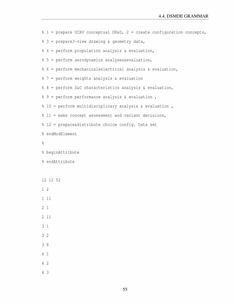
4.4. DSMDE GRAMMAR

% 1 = prepare UCAV conceptual DR&O, 2 = create configuration concepts,

% 3 = prepare3-view drawing & geometry data,

% 4 = perform propulation analysis & evaluation,

% 5 = perform aerodynamics analyses&evaluation,

% 6 = perform mechanical&electrical analysis & evaluation,

% 7 = perform weights analysis & evaluation

% 8 = perform S&C characteristics analysis & evaluation,

% 9 = perform performance analysis & evaluation ,

% 10 = perform multidisciplinary analysis & evaluation ,

% 11 = make concept assessment and variant decisions,

% 12 = prepare&distribute choice config. Data set

% endModElement

%

% beginAttribute

% endAttribute

12 12 52

1 2

1 11

2 1

2 11

3 1

3 2

3 8

4 1

4 2

4 3

55

4.4. DSMDE GRAMMAR

4 5

4 8

5 1

5 2

5 3

5 7

Example 4.4. [15]

%%MatrixMarket DSM 1 Coordinate Symmetric 4 Integer Integer Integer Integer IR

%

% Product Architecture Composite DSM Model of an automobile climate system

% Example 3.1.1;[Steven D Eppinger and Tyson R Browning;



% Number of interaction attributes: 4


%

% beginDomain


% endDomain

%

% beginModElement

% 1 = radiator, 2 = engine fan, 3 = heater core,

% 4 = heater hoses, 5 = condenser,

% 6 = compressor, 7 = evaporator case,

% 8 = evaporator core, 9 = accumulator,

% 10 = refrigeration controls, 11 = EATC controls,

% 12 = sensors, 13 = command distribution, 14 = actuators,

56

4.4. DSMDE GRAMMAR

% 15 = blower controller, 16 = blower motor

% endModElement

%

% beginAttribute

% Spatial,S=1; Eneregy,E=2; Information,I=3; Material,M=4;

% endAttribute

16 16 68

2 1 2 0 0 2

5 1 2 -2 0 0

5 2 2 0 0 2

13 2 0 2 0 2

4 3 1 0 0 0

7 3 2 0 0 0

8 3 -1 0 0 0

16 3 0 0 0 2

9 4 -1 0 0 0

6 5 0 2 0 2

8 5 -2 2 0 2

8 6 0 2 0 2

Example 4.5. [15]

%%MatrixMarket MDM 2

%%MatrixMarket DSM 1 Coordinate General 0 Pattern IR

%%MatrixMarket DSM 1 Coordinate Symmetric 0 Pattern IR

%%MatrixMarket DMM 1 Coordinate General 0 Pattern

%

% MDM model of BMW’s hybrid vehicle starter/generator architecture

57

4.4. DSMDE GRAMMAR

% including two DSM domains-components and functions and a DMM

% Example 8.1 ; Steven D Eppinger and Tyson R Browning;


%


%

% This model is a MDM (Multi-Domain Matrix) consisting of two DSM and

% One DMM (Domain Mapping Matrix) relating two DSMs.

% DMM maps the domain of one DSM to the domain of another DSM.

% The First DSM is a 19X19 matrix; The Second DSM is a 27X27 matrix;

% The resulting DMM is a 19X27 matrix in block row-major order.

%

% A = [ A11 A12;0 A22]

% A11: DSM 1

% A22: DSM 2

% A12: DMM 1

%

% Domain 1 (DSM 1):

% Number of attributes: 0


%

% beginDomain

% Product-Functions DSM

% endDomain

%

% beginModElement

%

58

4.4. DSMDE GRAMMAR

% 1 = Store Fuel, 2 = Store Electric Energy,

% 3 = Convert Fuel into Mech. Energy,

% 4 = Convert Mechanical into Energy,

% 5 = Convert Electrical into Mech. Energy,

% 6 = Deliver (Recover) torque to (from) wheels,

% 7 = Convert Moment transferred, 8 = Equate Rotation,

% 10 = Couple/Uncouple Moment,11 = Release Energy as Heat,

% 12 = Transfer Heat (to cooling system),

% 13 = Transfer Moment to (from) the Road,

% 14 = Slow or Stop Vehicle(recovering energy),

% 15 =Slow or Stop Vehicle(friction), 16 = Control Energy Flow,

% 18 = Consume EI. Energy for Auto Accessory OPS,

% 19 = Consume Mech. Energy for Engine Accessory

%

% endModElement

%

% beginAttribute

% endAttribute

%

% Domain 2 (DSM 2):

% Number of attributes: 0


%

% beginDomain

% Product-Component DSM

% endDomain

%

59

4.4. DSMDE GRAMMAR

% beginModElement

%

% 1 = Fuel Tank, 2 = High Voltage Battery, 4 = Internal Combustion Engine,

% 5 = E-Motor/Generator1, 11 = Transmission, 13 = Differetial Gear,

% 18 = Clutch Direct Coupling1, 21 = Cooling System, 22 = Wheels,

% 23 = Brake-system, 24 = Power Electronics/Inverter,

% 26 = Additional Electric Accessories, 27 = Mechanical Accessories

%

% endModElement

%

% beginAttribute

% endAttribute

%

% beginDomain

% Function-Component DMM

% endDomain

% beginModElement

% DMM 1 represents mapping between DSM 1 and DSM 2

% DMM 1 has 19 Rows and 27 Columns.

% endModElement

% beginAttribute

% endAttribute

%

19 19 42

1 3

2 12

60

4.4. DSMDE GRAMMAR

2 16

3 4

3 12

3 19

4 12

4 16

5 3

5 10

5 12

5 16

6 7

6 13

6 14

6 15

7 6

7 8

7 10

7 13

7 14

8 7

8 13

8 14

10 4

10 7

10 14

12 11

13 6

61

4.4. DSMDE GRAMMAR

13 7

13 8

13 15

14 16

15 6

15 11

15 13

16 2

16 4

16 5

16 12

16 14

16 18

27 27 15

1 4

2 21

2 24

4 5

4 21

4 27

5 18

5 21

5 24

11 13

11 18

13 22

62

4.4. DSMDE GRAMMAR

21 24

22 23

24 26

19 27 24

1 1

2 2

3 4

4 5

5 5

6 13

7 11

7 13

8 13

10 18

11 22

11 23

12 2

12 4

12 5

12 24

13 22

14 5

14 22

15 22

15 23

16 24

63

4.4. DSMDE GRAMMAR

18 26

19 27

64

Chapter 5

Conclusion

In this thesis, we (formally) propose a Data Exchange file format that is suitable for stor-

ing DSM and MDM data. At present there does not exist a common standard to share

DSM/MDM data. We believe that our standardized DSMDE format will significantly fa-

cilitate research and development of DSM modeling techniques by making data available

more widely than currently possible.

In Chapter 4, we have described each section of our proposed DSMDE file format along

with the existing base Matrix Market(MM) format. Additionally, we have provided the ex-

tended BNF (EBNF) description for the detail specification of our DSMDE format. Finally,

we have presented some important DSM model examples in our file format.

In this thesis, we have also analyzed six types of dependency such as call, set, uses, mod-

ifies and inits of three scientific software libraries named ADOL-C, CPPAD and CSparse

using the source code analysis tool Understand to generate DSMs for each dependency

type.

Future Research Directions: For future work, we consider the following enhancements

of the work presented in the thesis.

1. Input and Output. Although the DSMDE exchange format does not require any spe-

cial software to read and write model data, in practice, some software support is

typically provided to perform input and output. We are currently developing code in

C++ and MATLAB that can perform simple input and output.

2. Software Tools. A powerful feature of DSM modeling techniques is the visual rep-

resentation of features of the underlying model. For example, after a sequencing

65

5.0. CONCLUSION

analysis, the strongly connected components of the underlying directed network in a

time-based DSM can be concisely displayed and easily recognized as upper triangu-

lar blocks in the matrix form of the model. Visualization tools that are easy to use

and can display complex DSM data will be helpful to managers. This is an under

researched but promising area for future developments.

66

Bibliography

[1] A Graph and Matrix File Format description. http://people.sc.$\$fsu.edu/

˜jburkardt/data/hb/hb.html. Accessed: 2015-08-01.

[2] Compressed Column Storage description. http://netlib.org/linalg/html_templates/node92.html. Accessed: 2015-08-01.

[3] CSparse description. https://people.sc.fsu.edu/˜jburkardt/c_src/csparse. Accessed: 2015-07-24.

[4] DSM; helping to see complexity description. http://executive.mit.edu/blog/the-design-structure-matrix-helping-to-see-complexity-in-systems.Accessed: 2015-06-21.

[5] PERT,CPM and GANTT description. http://theconstructor.org/constrution/const-management/pert-cpm-and-gantt-chart/94/. Accessed:2015-07-20.

[6] Sparse Matrix description. http://people.sc.$\$fsu.edu/˜jburkardt/data/hb/hb.html. Accessed: 2015-08-01.

[7] Trillions and SciDAC description. http://trilinos.sandia.gov/;http://www.scidac.gov. Accessed: 2015-07-24.

[8] Khalid Alemerien and Kenneth Magel. Experimental evaluation of static source codeanalysis tools. page 1, 2013.

[9] J Bartolomei, M Cokus, J Dahlgren, R de Neufville, D Maldonado, and J Wilds.Analysis and applications of design structure matrix, domain mapping matrix, andengineering system matrix frameworks. Massachusetts Institue of Technology, 2007.

[10] B Bell. Cppad: a package for differentiation of c++ algorithms. 2008 06-01].http://www. coin-or. org/CppAD, 2011.

[11] Ronald F Boisvert, Roldan Pozo, and Karin A Remington. The matrix market ex-change formats: initial design. National Institute of Standards and Technology Inter-nal Report, NISTIR, 5935, 1996.

[12] Tyson R Browning. Applying the design structure matrix to system decompositionand integration problems: a review and new directions. Engineering Management,IEEE Transactions on, 48(3):292–306, 2001.

[13] Iain S Duff, Roger G Grimes, and John G Lewis. Sparse matrix test problems. ACMTransactions on Mathematical Software (TOMS), 15(1):1–14, 1989.

67

http://people.sc.$\$fsu.edu/~jburkardt/data/hb/hb.html


http://netlib.org/linalg/html_templates/node92.html

http://netlib.org/linalg/html_templates/node92.html

https://people.sc.fsu.edu/~jburkardt/c_src/csparse

https://people.sc.fsu.edu/~jburkardt/c_src/csparse

http://executive.mit.edu/blog/the-design-structure-matrix-helping-to-see-complexity-in-systems

http://executive.mit.edu/blog/the-design-structure-matrix-helping-to-see-complexity-in-systems

http://theconstructor.org/constrution/const-management/pert-cpm-and-gantt-chart/94/

http://theconstructor.org/constrution/const-management/pert-cpm-and-gantt-chart/94/



http://trilinos.sandia.gov/; http://www.scidac.gov

http://trilinos.sandia.gov/; http://www.scidac.gov

5.0. CONCLUSION

[14] Steven D Eppinger. A planning method for integration of large-scale engineeringsystems. pages 199–204, 1997.

[15] Steven D Eppinger and Tyson R Browning. Design structure matrix methods andapplications. MIT press, 2012.

[16] Andreas Griewank, David Juedes, and Jean Utke. Algorithm 755: Adol-c: a packagefor the automatic differentiation of algorithms written in c/c++. ACM Transactionson Mathematical Software (TOMS), 22(2):131–167, 1996.

[17] Robert A Hanneman and Mark Riddle. Introduction to social network methods. 2005.

[18] Shahadat Hossain, Ahmed Tahsin Zulkarnine, et al. Design structure of scientificsoftware–a case study. 2011.

[19] Diane Kelly and Rebecca Sanders. Assessing the quality of scientific software. 2008.

[20] Andrew Kusiak and Juite Wang. Efficient organizing of design activities. The Inter-national Journal Of Production Research, 31(4):753–769, 1993.

[21] Udo Lindemann. Home dsmweb. org.

[22] Alan MacCormack, John Rusnak, and Carliss Y Baldwin. Exploring the structure ofcomplex software designs: An empirical study of open source and proprietary code.Management Science, 52(7):1015–1030, 2006.

[23] Osni Marques and Tony Drummond. Building a software infrastructure for computa-tional science applications: lessons and solutions. pages 40–44, 2005.

[24] Thomas Udo Pimmler and Steven D Eppinger. Integration analysis of product decom-positions. 1994.

[25] Ingvar RASK and Staffan Sunnersjo. Design structure matrices for the planning ofrule-based engineering systems. 8:349, 1998.

[26] Amira Sharon, Dov Dori, and Olivier De Weck. Model-based design structure matrix:deriving a dsm from an object-process model. pages 1–12, 2009.

[27] Kaushik Sinha and Olivier L de Weck. Structural complexity metric for engineeredcomplex systems and its application. pages 181–194, 2012.

[28] Scientific Toolworks. Inc., understand for java: User guide and reference manual.2005)[2011-03]. http://www. scitools. com, 2005.

[29] Andrea Walther, Andreas Griewank, and Olaf Vogel. Adol-c: Automatic differentia-tion using operator overloading in c++. PAMM, 2(1):41–44, 2003.

[30] A Yassine. An introduction to modeling and analyzing complex product developmentprocesses using the design structure matrix (dsm) method. Urbana, 51(9):1–17, 2004.

[31] Ahmed Tahsin Zulkarnine. Design structure and iterative release analysis of scientificsoftware. 2012.

68

design structure matrix : models, applications and data …

Documents