Designing a Flue Gas Condenser System for Lomma Power Plant

KET050: Feasibility Studies on Industrial Plants

Per Nobel, Marilia Vasconcelos, Fredrik Tegnér, Ferran Pérez Serrano

5/17/2014

2

Executive Summary The fitting of a flue gas condenser unit to a biofuel powered boiler can increase the overall

power plant efficiency substantially as the sensible and latent heat of moist flue gases is

recovered. In this report, the flue gas condenser at the new wood-fired power plant at Örtofta

is evaluated. The findings of the operating conditions and used design are then implemented

when designing a similar flue gas condenser unit for the smaller boiler at the power plant of

Lomma. The process is evaluated using three different compositions of fuel ratios of wood

chips and demolition wood. Appropriate operating conditions and design variables were

found through solving a systems of equations with energy and mass balances over the

combustion process, using MATLAB R2012a©

.

In addition, the treatment of condensate from the condenser was considered. Through the pre-

treatment of condensate using membrane technology, condensate can be used as make-up

water for the boiler and the district heating network using the existing treatment facility at the

Lomma plant. Thus, the consumption of city water for this purpose can be reduced.

The cost estimation for the project was performed by three different methods showing similar

results and both net present value and pay off times were calculated. According to the Ulrich

manual method the pay off time will be 45.1 years when using wood chips only (case 1).

When using 50 % each of wood chips and demolition wood, the pay off time is 4.66 years

(case 2). The best choice is using demolition wood only (case 3) since the pay of time is only

2.56 years. This option also implies the best annual income and net present value for the

investment. This is due to the increased energy output when using wood chips not making up

for the increase in the fuel cost.

3

Acknowledgements We would like to thank SEKaftringen for giving us the opportunity to study the flue gas

condenser unit at the Örtofta plant. We feel that we have learnt a lot about flue gas

condensing when designing for a similar unit at the Lomma plant, but especially we have

received some experience in real process design. We would especially like to thank Marie

Caesar for enthusiastically presenting the two power plants and for giving answers to tricky

technical questions and information requests. We also would like to give special thanks to

Prof. Stig Stenström, our tutor, for supporting us in every way and discussing the

thermodynamics of combustion. We thank Prof. Ann-Sofi for here expert correspondence in

membrane technology and condensate treatment. Finally, we would like to thank Prof. Hans

T. Karlsson on any information on the art of wet scrubbing and saturation of hot flue gases.

4

Table of symbols

Symbol Unit Definition

LATIN SYMBOLS

a SEK/year Annual net payment

A m2 Heat transfer area

ALomma m2 Quench cross section area in Lomma

Amembrane m2 Membrane area

AÖrtofta m2

Quench cross section area in Örtofta

CBM,$ US$ Cost in united states dollars

CBM,SEK SEK Cost in SEK

CFeed ppm Concentration of the feed going into the membrane

Cp US$ Purchased equipment cost

Cp,i J/kg·K Specific heat

CPermeate ppm Concentration of the permeate leaving the membrane

D hours/year Plant operating time a year

Fbp,rec l/s Water flow bypassed to the recipient

Fcond l/s Water flow from the flue gas condensate

FFeed l/s Water flow to the RO-Feed tank

Fpermeate l/s Membrane permeate flow

Fquench l/s Water flow back to the quench

Fα

BM - Cost factor

G m3/s Actual flue gas flow rate in the quench

g Nm3/s Gas flow rate

Ginv SEK Year zero investment

g0 Nm3/s Flue gas

g0,H2O Nm3/s Water in the flue gas

g0,i Nm3/s Flue gas of component i

g0t Nm3/s Dry flue gas

gH2O,quench Nm3/s Required water in the quench

h kJ/kg Specific enthalpy

HF,G MJ/kg Enthalpy of the flue gas entering the quench

Hi MJ/kg Effective heat value

HS MJ/kg Calorimetric heat value

HS,C MJ/kg Calorimetric heat value from carbon

HS,H MJ/kg Calorimetric heat value from hydrogen

I SEK/year Annual income

i - Interest rate

ICE - Chemical engineering plant cost index

Icur SEK/US$ Currency exchange index

J l/s· m2

Membrane flux

k W(m2K) Heat transfer coefficient

L l/s Liquid flow ratio

L/G l/m3

Liquid to gas flow ratio

L0t,excess Nm3/s Excess dry air

ṁ kg/s Mass flow of fuel to the boiler

5

ṁcondensate kg/s Condensate mass flow

ṁD.H kg/s District heat mass flow

ṁquench kg/s Mass flow of required water in the quench

np years Pay off time

nv 106·SEK Net present value

O2,out - Percentage of oxygen in the flue gas

P MJ/kg Boiler energy output

pD.H. SEK/MWh District heating price

pH2O Pa Partial pressure of water

Pin Pa Pressure at the membrane inflow

Pout Pa Pressure at the membrane outflow

Ppermeate Pa Pressure at the permeate

Q J Heat

gH2O,max Nm3/s Maximum amount of water in the flue gasses

R - Retention

RRO - Retention of conductivity for RO-membranes

T K Temperature

TD.H K District heat temperature

TF.G. K Temperature of the flue gas

TMP Pa Transmembrane pressure

U SEK/year Expenses

vquench m/s Flue gas velocity in the quench

VR - Volume reduction

zcone m Height of quench conical part

GREEK SYMBOLS

xi - Fraction of component i

xmoist - Moist fraction

ΔHVAP J/kg Water enthalpy of vaporization

ΔTln K Logarithmic temperature difference

ΔP SEK Price difference

η - Boiler efficiency

ρ kg/m3 Density

σcond μS/cm Conductivity of the flow from the condensate

σFeed μS/cm Conductivity of the flow to the RO-Feed tank

σp,i μS/cm Conductivity of the permeate after membrane step “i”

ϕ m Quench diameter

6

Table of Contents Executive Summary ...................................................................................................................... 2

Acknowledgements ...................................................................................................................... 3

Table of symbols .......................................................................................................................... 4

Part I - Introduction ...................................................................................................................... 9

1.1 Project objectives ........................................................................................................................ 10

1.2 Method ........................................................................................................................................ 10

Part II – Theoretical Background ................................................................................................. 12

2.1 Effects of boiler fuels and boiler load on flue gas condenser operation .................................... 12

2.2 Condenser design options with cost estimations ....................................................................... 13

2.2.1 Theoretical considerations involved in designing a heat exchanger.................................... 14

2.2.2 Implementing a condenser to an existing plant: a case study review ................................ 16

2.2.3 Dehumidifying condenser .................................................................................................... 18

2.3 Flue gas cleaning and particle removal. ...................................................................................... 19

2.4 Condensate treatment and boiler water production at power plants ....................................... 20

2.4.1 Using membrane technology for condensate cleaning. ....................................................... 21

2.5 Alternative methods for the condensation of flue gases ............................................................ 22

2.5.1 Venturi scrubbers – efficient particle collectors .................................................................. 23

2.5.2 Direct and indirect heat exchange of flue gases .................................................................. 24

2.5.3 Membrane technology for flue gas processing .................................................................... 25

2.5.4 Introducing heat pumps with a flue gas condenser unit ...................................................... 27

Part III - Calculations ................................................................................................................... 29

3.1 Material calculations ................................................................................................................... 29

3.1.1 Material composition ........................................................................................................... 29

3.1.2 Material energy calculations ................................................................................................ 29

3.2 Flue gas calculations .................................................................................................................... 30

3.2.1 Flue gas composition calculations ........................................................................................ 30

3.2.2 Flue gas energy calculations ................................................................................................. 31

3.3 Quench basic calculations ........................................................................................................... 31

3.3.1 Quench temperature ............................................................................................................ 31

3.4 Condenser basic calculations ...................................................................................................... 32

3.4.1 Condenser energy balance ................................................................................................... 32

3.5 Condensate water calculations ................................................................................................... 33

3.5.1 Condensate flow ................................................................................................................... 33

7

3.5.2 Quench flow ......................................................................................................................... 33

Part IV - Designing the Flue Gas Condenser Unit for Lomma Power Plant .................................... 34

4.1 Quench dimensions ..................................................................................................................... 35

4.1.1 Liquid-to-gas flow ratio ........................................................................................................ 36

4.2 Preliminary thermal design of the condenser ............................................................................. 37

Part V - Design for the Treatment of Condensate Water at the Lomma Plant................................ 41

5.1 Make-up water production at Lomma today .............................................................................. 41

5.2 Treatment of condensate for make-up water production at Örtofta ......................................... 42

5.2 Proposed design for the condensate water treatment at Lomma Power Plant ............................. 43

5.2.1 Design calculations for the pre-treatment of condensate at Lomma .................................. 44

5.2.2 Membrane area estimations .................................................................................................... 45

Part VI – Estimation of Costs ....................................................................................................... 47

6.1 Investment ................................................................................................................................... 47

6.1.1 Quench ................................................................................................................................. 47

6.1.2 Condenser............................................................................................................................. 47

6.1.3 Water treatment .................................................................................................................. 47

6.2 Income & expenses ..................................................................................................................... 48

6.3 Results ......................................................................................................................................... 49

6.3.1 Pay off method ..................................................................................................................... 49

6.3.2 Net present value ................................................................................................................. 49

6.4 Sensitivity analysis ....................................................................................................................... 50

6.4.1 Condenser outgoing temperature changes .......................................................................... 50

6.4.2 Fuel price changes ................................................................................................................ 50

Part VII – Discussion & Conclusions ............................................................................................. 52

7.1 Alternative methods for the condensation of flue gases ............................................................ 52

7.1.1 Venturi scrubbing ................................................................................................................. 52

7.1.2 Flue gas condensation with membranes .............................................................................. 52

7.1.3 Direct and indirect heat exchange of flue gases ................................................................... 52

7.1.4 Heat pump ............................................................................................................................ 52

7.2 Design considerations ................................................................................................................. 53

7.2.1 Quench design ...................................................................................................................... 53

7.2.2 Condenser design ................................................................................................................. 53

7.2.3 Design for the treatment of condensate .............................................................................. 53

7.3 Case investment evaluation ........................................................................................................ 54

8

7.4 Conclusions .................................................................................................................................. 55

Part VIII – Appendix .................................................................................................................... 58

9.1 Fuel data sheet ............................................................................................................................ 58

9.2 Overall process sheet for the flue gas condenser at the power plants of Örtofta and Lomma. 59

9.3 Örtofta combustion/boiler .......................................................................................................... 60

9.4 Örtofta quench ............................................................................................................................ 61

9.5 Örtofta condenser ....................................................................................................................... 62

9.6 Lomma case 1 overall balance..................................................................................................... 63

9.7 Lomma case 2 overall balance..................................................................................................... 64

9.8 Lomma case 3 overall balance..................................................................................................... 65

9.9 Present configuration for boiler water production at the Lomma plant .................................... 66

9.10 Condensate treatment and boiler water production at the Örtofta plant. .............................. 67

9.11 Proposed design for Lomma condensate treatment and boiler water production. ................. 68

9

Part I - Introduction

The aim of the following report is to design an implementation of a flue gas condenser unit in

the biomass fired boiler energy plant situated in Lomma, in order to recover heat from the gas

stream and increase the plant efficiency.

For this purpose the current flue gas condenser unit installed at the Örtofta power plant, which

also uses biomass, is to be examined.

The main advantage of biomass fired boilers is that they use a renewable source of energy as

opposed to fossil fuel fired boilers. There are several fuels that are considered biomass

(agricultural waste, wood, landfill gases). In the power plant in Örtofta wood chips,

demolition wood and peat are being used in different mixtures.

Out of the 120,2 MW produced in the combustion chamber 10,9MW will be dedicated not

only to heat up the flue gases but also to evaporate the water content in them. Therefore a flue

gas condenser offers the possibility to recover a large sum of energy.

The purpose of the flue gas condenser units is to recover heat form the gaseous flue gas

streams leaving the plant. In order to do so the water contained in the stream is condensed.

Due to the high vaporization heat of water this allows a high energy recovery.

In the setup used in Örtofta the flue gas first enters a quench where it sprayed with water in

order to saturate the water content in the gas to increase the condensation efficiency, and then

this stream enters the condenser where it is first sprayed with water again and then heat

exchanged with the district heating network in order to heat up the water circulating in this

network. This condenser then produces water that can be treated in order to be used as make

up water for the boiler and the district heat network.

In order to study the feasibility of adapting this technology currently existing in Örtofta to the

Lomma power plant, the following report will study the design of the quench and the

condenser for the flue gas condensing unit and also the design of the water treatment process,

taking into account the different operating conditions at Lomma. Then, a cost estimation will

be performed for the proposed design in order to give an estimation of the cost of this

implementation.

10

1.1 Project objectives The objectives for the project are:

First to calculate the operating conditions of the flue gas condensing unit currently

operating in the Örtofta power plant, with the objective to recover as much energy in

the condenser as possible.

Then these same calculations will be applied for the power plant operating in Lomma.

The calculations must be adapted for the different flue gas composition in this power

plant and should be done for three different cases. This power plant is currently only

operating by using demolition wood as fuel but calculations should also be performed

for different mixtures of wood chips added to the demolition wood.

The next step is to design the flue gas condenser unit that should operate in the

Lomma power plant. This part should include the design of both a quench and the

condenser itself.

The present water treatment process, for the production of the boiler make up water

and district heat network make up water, will be redesigned. This process should use

the water obtained in the condenser in order to reduce the consumption of softened

city water.

Lastly a cost estimation of the project must be done to calculate the reliability of

implementing the flue gas condenser to Lomma återbruket.

1.2 Method As it has already been mentioned, the purpose of the study is to examine the feasibility of

implementing a flue gas condensing system at the power plant situated in Lomma. This will

be done by means of studying the power plant situated at Örtofta which already has a flue gas

condensing system. The principal idea of the flue gas condenser is illustrated in appendix 9.2.

Both power plants operate by burning biomass. In Örtofta this is mainly in the form of a

mixture of demolition wood and wood chips, on the other hand the Lomma power plant burns

only demolition wood. The possible benefit of using wood chips at Lomma will be also

studied at this report.

The main difference between both power plants is obviously the different size of both plants,

and total energy output. The plant situated at Örtofta produces 110 MW whereas the one

situated at Lomma produces only 16 MW of energy.

At Örtofta the power plant consist of a boiler where the biomass is fired to produce heat to

generate steam in the steam cycle for the production of electricity and/or district heat. Then

the flue gases coming out of the boiler are driven into the flue gas condensing unit. This unit

consists of a quench and a condenser.

First in the quench, the flue gas is humidified by means of spraying water into it. This helps

the later condensing of the water present in the flue gas at the condenser and also lowers the

temperature of the flue gases.

11

Then in the condenser the flue gases are heat exchanged with water coming from the district

network, thus transferring heat into the district heating network and condensing the water

present in the flue gas.

Both these units are to be studied and tuned down and designed for the Lomma power plant.

Also both plants have a water treatment system. Its purpose at Lomma is the production of

boiler make up water from softened city water but at Örtofta it also uses the condensate water

from the flue gas for the same purpose and the production of makeup water for the district

heat network. Thus, it contains equipment not present in Lomma such as ultrafiltration and

microfiltration steps that might be required in order to also treat the condensate produced in

Lomma if the flue gas condenser is to be installed.

All of the required calculations for the implementation at Lomma will be done considering

three different cases of fuel composition. One case will assume the use of only wood chips to

fire the boiler, the second case will consider the use of 50% wood chips 50% demolition

wood, and case 3 studies the use of only demolition wood as it is operating at the moment.

12

Part II – Theoretical Background There are several reasons for fitting boilers with flue gas condensers. Adding a condensing

flue gas heat exchanger to a boiler leads to an increase in the plant energy efficiency due to

the recovery of both sensible and latent heat. By lowering the flue gas temperature below the

dew point the water vapor can be condensed, recovering the latent heat released. Taking the

lower heating value as the basis for calculation, the efficiency can reach or even exceed

100%. The flue gas can have 15 to 40% of the fuel energy content [1]. Also, the condensed

flue gas water can be processed and used as boiler make up water.

Another reason for flue gas condensation is for emission reduction. For example, particle

emissions can be severely reduced through condensing heat exchangers. In Finland, about 25

% of the total direct 4.5 emissions, that is particles less than 2.5 micro millimeters, are from

wood combustion. The use of a condensing flue gas scrubber can lead to the removal of 44%

of 3.0 and 84% of total solid particles [2]. These emissions are expected to increase since the

use of renewable sources, like wood, increases for combustion processes. Small particles

imply a health risk since it can be hazardous to inhale them at higher concentrations [3].

At present, there is a lot of research in flue gas condensation and new inventions and

techniques are being developed. The current design at the plant at Örtofta is successful in the

recovery of flue gas heat, increasing the overall plant efficiency substantially. The question is

if the design is equally applicable to the much smaller heat and power plant in Lomma, using

similar fuels. Looking into scientific publications, this chapter brings forward important

matters of consideration for flue gas processing. Also, alternative techniques and methods are

presented and briefly evaluated.

2.1 Effects of boiler fuels and boiler load on flue gas condenser operation Blumberga et al [4] emphasize the EU goal of increasing the amount of renewable energy

sources to 20 % by 2020, and point out the efficient combustion of wood fuels as a

contribution in achieving this goal. It is also stressed that the moisture content of wood chip

fuels shall not exceed 25 % according to EU standards. For the Lomma plant, the moisture

content is clearly a strict fuel quality parameter; the higher the moisture content, the more heat

will be devoted to evaporate the moisture and less heat can be allocated to steam production.

Thus, a high moisture content of the fuel implies an ineffective heat production process. On

the other hand, for a plant with flue gas heat recovery, like Örtofta, one should also keep in

mind that a moist fuel will give flue gases with high energy content which can be recovered in

the flue gas condensation unit.

Based on experiments performed on a commercial scale plant, Blumberga et al [4] evaluated

the correlation between total specific heat recovered in a gas condenser and the load on the

boiler. It is found that as the boiler load increases, the amount of heat energy recovered per

unit of produced heat decreases. This can partly be explained by condensation limitations. An

interpretation is that it is important to dimension the flue gas heat recovery system to the

capacity of the boiler in order to ensure an effective heat recovery and plant efficiency, which

seems intuitive. The authors find that for the evaluated plant, it is possible to recover heat

13

energy in the range of 100-180 kWh/MWh of produced heat in the boiler. It is thus important

to know the overall boiler load throughout the year in order to adapt the condenser type and

surface area for efficient heat recovery. Appropriate condenser surface area evaluations and

material alternatives are further evaluated in section 4.2.

2.2 Condenser design options with cost estimations When designing heat exchangers some factors need to be taken in consideration. In a

condenser heat will be transferred through conduction and convection. For large Reynolds

numbers, the energy transferred will be mostly by convection. As a condenser is being

designed, both the latent and sensible heat is of interest [5]. In a condenser, there is phase

change, and transfer of latent heat. The rate of phase change is dependent on the rate of heat

transfer, on the rate of nucleation of drops and on the behaviour of the new phase. The

condensation process can vary depending on the composition of the vapour; however, the

temperature will only be constant if a few conditions are met. The vapour must be a single

component vapour, not superheated, and not sub cooled below condensing temperature. The

condensing temperature is determined by the pressure in the shell side, which, considering

there are only small friction losses in the process can be considered constant [6].

The addition of a condenser to the plant will lead to an increase in the investment costs. The

costs can vary with the heat exchanger material and area needed; the setting of the material;

the increase in the power consumption caused by an added resistance; extra piping and valves;

manufacture, installation maintenance and repair costs [1]. The design and installation of the

condenser can influence the performance observed in the plant [2]. However, installing a

condenser will save energy and the payback time could be estimated for a natural gas fired

boiler to be between 3 to 4,5 years [1], for a biomass fired boiler this period can vary between

2 and 7 years [2] – with great influence from the chosen material for the heat exchanger. If the

exiting flue gas temperature is decreased too much it can lead to an increase in the needed

heat exchanger area, increasing the installation costs and thus the payback time. Due to the

slightly acid nature of the condensate this material needs to be resistant to corrosion. It is of

interest to have the largest possible difference of temperature between the boiler and the

return water. The amount of recovered heat can vary with the season and geographic location

as the temperature of the return water changes. [1]

Chen et al [2] evaluated the technical and economic feasibility of using condensing boilers in

a large district heating system. In order to avoid the corrosion that usually accompanies the

use of low temperature heat, using a corrosion resistant material is necessary. The recovery of

the latent heat improves the thermal efficiency, especially when dealing with lower excess air

ratios, as increasing the excess air decreases the vapour partial pressure, lowering the dew

point, and thus the amount of condensable water. The formation of the condensate can help in

the reduction of particles emissions as it removes most of the particulates generated with the

combustion. [2]

The return water temperature is directly related to the boiler efficiency, as it will determine

how much latent heat can be captured and how much vapour is condensed. Higher

temperatures mean that less vapour condenses. This temperature must be below the dew point

14

of the condensable gas. If the return water cannot be used directly as a heat sink a heat pump

can be added. [2] The addition of a heat pump is further discussed in section 2.5.4 (high

energy use and increase in capital costs).

2.2.1 Theoretical considerations involved in designing a heat exchanger

In order to solve heat transfer problems it is necessary to resolve the energy balances and to

estimate the rates of heat transfer. Considering operation at steady state; there is no shaft

work, negligible potential, mechanical and kinetic energies. Thus (neglecting the heat transfer

into the outside environment) the energy balance can be given by the overall enthalpy balance

(equation 2.1). Equation 2.2 gives the balance for a condenser, with transfer of both sensible

and latent heat; considering saturated vapour at the inlet and vapour at condensing

temperature on the outlet [6].

(2.1)

(2.2)

In order to simplify the calculations of the heat flux and of the heat transfer coefficients, the

average temperature of the cross section profile can be considered as the temperature of the

stream. The heat flux is proportional to the driving force (the temperature difference between

the streams), and the driving force varies along the tube. The heat flux also changes

throughout the tube.

(2.3)

The local overall heat transfer coefficient varies with the fluids temperatures, but if the

temperature ranges are reasonable, it can be considered constant, and equation 2.3 can then be

integrated to find equation 2.4, that can be used to predict the performance of a heat

exchanger or to calculate the area needed in a new heat exchanger [6].

(2.4)

The heat transfer coefficient for heat transfer between a moving fluid and a solid surface

depends on the thermal conductivity and on the thickness of the fluid film. The thickness of

the fluid film will vary depending on the fluid properties, velocity and the type of fluid flow.

By making some assumptions (within reason) approximate solutions can be calculated. Some

compromises must be made in order to achieve the best possible outcome, as for a set heat

transfer rate, if the fluid velocity is low, less power is required; however, a higher surface area

is needed. [5].

Condensation can happen in drop wise or film-type. In film-type condensation, the liquid

condensate forms a continuous layer in the surface of the tubes – this layer gives the

resistance to the flow of heat). In drop wise, the condensation happens at microscopic

nucleation sites, with growth of the droplets to form rivulets and then an extremely thin film

with very low thermal resistance. Drop wise condensation has higher heat transfer coefficients

than film-type condensation. Despite this fact, it is harder to establish the conditions for drop

15

wise condensation through the entire length of the tube, especially for steel. For this reason,

the condensing will be modelled assuming film-type condensation [6].

The coefficients for film-type condensation are calculated assuming that the liquid is at

condensing temperature and neglecting super-heat of the vapour. The Nusselt equations give

the rate of heat transfer in film-type condensation, with the vapour and liquid in

thermodynamic equilibrium. Some assumptions about the layer of condensate need to be

made: the flow is laminar and downwards; there is no velocity at the wall; the temperatures at

the wall and of the vapour are constant; and that the velocity of the outside layer of the film is

independent of the velocity of the vapour. The average heat transfer coefficient for the local

tube is three quarters of the local coefficient at the bottom of the condenser. The local

coefficient can be calculated using equation 2.5 and 2.6, taking the properties at the average

film temperature (2.7) [6].

(2.5)

(2.6)

(2.7)

Individual resistances are added to find the overall resistance (combined resistances in series).

When considering a heat flux between two fluids separated by a wall, there are three

temperature profiles to be taken into consideration. The resistance of the wall is usually small.

The fluid resistances are correlations for individual heat transfer coefficients or film

coefficients. To calculate the overall coefficient the individual coefficients are added in the

same equation:

(2.8)

However, the areas vary for the individual coefficients of each tube, as the fluid inside the

tube uses the inner area of the tubes, the fluid outside uses the outer area and the resistance of

the wall uses a logarithmic mean of both areas. To define one overall coefficient for the

system it is necessary to base the heat transfer rate in either the inside or the outside area of

the tubes. Equation (2.9) shows the overall heat transfer coefficient for the outside area of the

tubes:

(2.9)

In order to simplify the calculations, the area of the side with the highest resistance (lowest h)

can be used. Assuming that the fouling effects are negligible, and that one h is much larger

than the other the overall coefficient can be given by:

(2.10)

16

To calculate the coefficients for the tube side and for the shell side there are some correlations

that can be used for each case that takes in consideration the flow and fluid properties of each

side. As the coefficients are calculated using temperature dependant fluid properties and there

are temperature variations associated with the heat exchange, it is logic to say that the values

of the coefficients vary throughout the condenser. However, if the coefficient varies less than

by a factor of 2:1, an averaged value can be used to find the overall coefficient. For the shell

side, the calculation is more complex as it has to take in consideration the presence of baffles

and the area occupied by the tubes [6].

The deposition on the surface of the tubes of solids, scale and dirt, among other components

(present in the fluids doing the heat exchange) lead to an added resistance called fouling

resistance. This reduces the overall coefficient. A term for the fouling resistance should be

added to the total thermal resistance for each side of the tube. [5, 6]

When designing a shell-and-tube heat exchanger the choice of which fluid will pass through

the tubes and which will go through the shell must be made. Corrosive fluids should go on the

inside of the tubes, so that only the inside of the tubes have to be of a corrosive resistant

material; very hot fluids should also go on the inside of the tubes to reduce heat loss to the

ambient; and dirty fluids that will lead to the formation of deposits and fouling should also be

on the inside as it is easier to clean, mixtures of condensable and non-condensable gases can

also go on the inside of the tubes. Viscous fluids are usually on the shell side as to increase

flow velocity and turbulence. Still, the final decision of the fluids side is done by considering

which arrangement gives the higher overall coefficient and the lower pressure drop. [6,15]

2.2.2 Implementing a condenser to an existing plant: a case study review

In Chen’s et al case study [2] the heat exchanger evaluated was an indirect contact shell and

tube heat exchanger, appropriate for liquid-to-liquid and liquid-to-phase change heat transfer

applications and also for high pressure differences. The flue gas goes through the shell-side

and the return water through the tube-side of the heat exchanger. When designing the heat

exchanger the optimum between high heat transfer coefficients and minimum pressure drop is

of interest. A lower diameter can increase the heat exchanger coefficients leading to more

compact heat exchangers, which in turns mean higher pressure drops. Two materials were

evaluated for the heat exchanger: stainless steel and carbon steel, some of the most common

materials for heat exchangers. In order to use carbon steel it is necessary to coat the surfaces

with a corrosion resistant material, which in this study was polypropylene. Before the heat

exchanger the flue gas goes through a pre-treatment to remove particles [2].

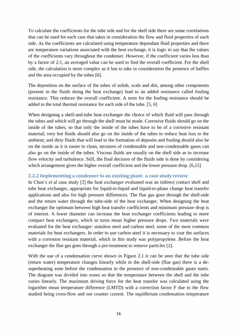
With the use of a condensation curve shown in Figure 2.1 it can be seen that the tube side

(return water) temperature changes linearly while in the shell-side (flue gas) there is a de-

superheating zone before the condensation in the presence of non-condensable gases starts.

The diagram was divided into zones so that the temperature between the shell and the tube

varies linearly. The maximum driving force for the heat transfer was calculated using the

logarithm mean temperature difference (LMTD) with a correction factor F due to the flow

studied being cross-flow and not counter current. The equilibrium condensation temperature

17

decreases as the water vapour condenses, reducing the temperature difference between the

shell and tube side [2].

In the plant at Örtofta the flue gases go through the quench and are humidified and cooled

before entering the condenser. Due to this, the de-superheating part shown figure 1 does not

apply for the case studied. At Örtofta the flue gas enters the condenser at a temperature of

approximately 65°C and leaves at 45°C. In Lomma this same temperature difference is

maintained when designing the plant. However, at the plant in Örtofta, the flue gas flows

inside the tubes while the return water goes on the shell side.

Figure 2.1: Condensation curve for the flue gas in a shell and tube heat-exchanger [2].

In order to adequately estimate the surface area of the heat exchanger a thermal design should

be done, finding the heat transfer coefficients. The presence of non-condensable components

in the flue gas should be taken in consideration. The correlation used in the tube side

considered fully developed turbulent flow in smooth tubes in order to find the heat transfer

coefficient. On the shell-side the heat resistances due to the condensate film and to the cooling

of the sensible heat of the flue gases were considered, and the thermal resistance of the gas

stream (the inverse of the heat transfer coefficient of the gases) and the resistance of the

condensate film were calculated (for zones II – IV).

Fouling effects are expected in condensing boilers, both inside and outside the tubes.

However, since it is a time dependent problem, for the design of the heat exchanger a fixed

value should be used. In this case study, due to the polymeric coating, carbon steel has a

higher thermal resistance than stainless steel. The thermal resistances for both condensers are

higher on the shell-side, especially before the condensation starts. To determine the overall

heat transfer coefficient, first the local overall coefficient from the shell to the tube side can be

calculated. These can then be used to find the coefficients at the boundaries of each zone,

obtaining afterwards the mean overall heat transfer coefficient for each zone. After these

determinations the size of the condenser can then be determined as well as the heat flux that

ranges between 1.5 and 2.5 kW/m2 [2].

18

The pressure drop was calculated as it has great influence over the determination of the

necessary pumping power and fan work input, both of which incurs in extra operating and

capital costs. Due to the higher thermal resistance (caused by the polymeric coating), the

carbon steel condenser has longer tubes and larger surface area. Thus, the pressure drop is

also higher. The values for the pressure drop and the power for the pump and for the fan for

both types of heat exchangers are shown in Table 2.1 [2]. The pressure drop on the shell side

is high for both materials; this could be due to the condenser also being used to de-superheat

the flue gas before the condensation starts.

Table 2.1: Pressure drop and needed pump and fan power for carbon steel and stainless steel.

Pressure drop Pump power Fan power

Tube side Shell side Tube side Shell side

Stainless steel 3.2 kPa 28.4 kPa 0.43 kW 828.3 kW

Carbon steel 3.8 kPa 23.1 kPa 0.50 kW 993.4 kW

In the cost estimation the capital, equipment, installation, operating and maintenance costs

were estimated for both condensers. In the estimation of the operating and maintenance costs

the electricity consumption, the chemical treatment of the condensate and fouling removal

were considered, as well as an approximated 6% of fixed capital cost as the maintenance cost.

The stainless steel has a higher cost as material; however, the carbon steel condenser has

higher operating costs and higher electricity consumption. This leads to a total operating and

maintenance cost to be similar for both materials. Carbon steel has a lower life expectancy but

a shorter period for cash return; it also has less sensitivity to the change in interest rates. The

cash return is expected after 2 years for carbon steel condensers and 5 to 7 years for stainless

steel condensers [2].

2.2.3 Dehumidifying condenser

In a dehumidifying condenser, where a mix of condensable and non-condensable gases is

present, the vapour is condensed inside the tubes with the coolant flowing through the shell in

a vertical setup. This is the scheme used in Örtofta and an illustration of this can be seen in

Figure 2.2. In this figure there is use of baffles that increase turbulence, of a floating heat to

provide for the thermal expansion and a vapour liquid separating cone in order to ease the

separation of the condensate flow from the non-condensable gases and uncondensed vapour.

In this set up, the formation of stagnant inert gas regions is avoided [6].

For in tube condensation, the choices of correlation for the heat exchanger coefficient and for

other parameters must agree. If the flow has low velocities, the pressure drop along the tube

can be neglected, and the Nusselt correlation for laminar flow can be applied. In this case it is

possible to have vapour super-heat and presence of non-condensable. If the flow has high

velocity, though, the choice of the nondimensional parameters is harder, as the influence of

the gravity and of the vapour-shear must be known. It is hard to predict the pressure drop [15].

19

Figure 2.2: Dehumidifying cooler-condenser.

2.3 Flue gas cleaning and particle removal Whether or not the flue gases are to be condensed or let directly to the chimney, they should

be treated in a flue gas cleaning unit first. Ash, salt and smaller particles can cause fouling and

corrosion to the flue gas condenser unit and the chimney. In addition, emissions to the

environment should be kept below threshold levels.

A common technique for particle removal is a fabric bag house filter units. Figure 2.3 shows

the principle of this technique. The idea is that the unclean flue gases pass through to the

inside of the bag, leaving particles stuck on the bag outer surfaces. Therefore, a filter cake will

form on the surface after some time. To remove the filter cake, a pulse of high pressurized air

is let down the bag, causing the bag to be flexed and expanded. This will break up the cake

and particles will consequently fall to the bottom of the unit where they are collected and

removed. This type of bag house filter cleaning technique is referred to as “pulse-jet” or

“pressure-jet” cleaning [7].

20

Figure 2.3: Principle of fabric bag house filter unit for flue gas particle removal [7]

Particle removal units, like bag house filter units, are most often combined with flue gas

desulfurization units, FGD. In the FGD, lime reacts with the sulfuric content of the flue gases

where upon the sulfur precipitates into particulate matter. These particles are then separated in

the particle removal unit and removed.

2.4 Condensate treatment and boiler water production at power plants Introducing a flue gas condenser unit to a power boiler, one must of course consider the need

to clean the condensate. Even though most of pollutants and small particles are removed in

the flue gas cleaning and the quench, some of it will be dissolved in the condensate at the

condenser. The condenser is thus partly a flue gas cleaning step in itself. If the condensate is

let directly to a recipient, collected dust particles can cause unclear water and harm to the

aquatic life. Also considerate amounts of heavy metals can be present in the condensate,

although biofuels only give rise to modest levels. Therefore, the condensate should preferably

be filtrated before let to the recipient [8].

If the condensate is treated well enough, it can eventually be used as make-up water for the

steam cycle or at least for the district heating network. Usually, plants treat softened city

water for this purpose. Although not too expensive, an extensive use of city water implies

high costs in the long run. In addition, city water enters the water treatment unit at a low

temperature whereas the condensate is much warmer. Since make-up water needs to be pre-

heated, using condensate for this purpose has clear advantages in terms of energy.

The quality demands on boiler feed water are high. Especially, it is important that the water

has a low conductivity, i.e. contains low amounts of salts. This is also true for district heating

21

make up water, although the demands are not quite as high. Salts can cause corrosion of pipes,

heat exchangers, boiler equipment etc.

2.4.1 Using membrane technology for condensate cleaning.

Membrane technology encompasses a wide range of separation with regard to the size of

particles and solutes. Reverse osmosis-membranes (RO) have the finest pore-sizes and retards

dissolved salts [8]. However, the feed water to the RO-membranes should only contain very

small particles in order to ensure a good function of the membranes. If flue gas condensate is

used, it must thus be pre-treated to remove most of colloids and macromolecules [9, 10]. This

can be achieved through the introduction of coarser membranes prior to the RO-stage. One

option is to have microfiltration (MF) and ultrafiltration (UF) units coupled in series for RO-

feed water pre-treatment.

In order to be able to design for condensate treatment using membranes, one should be

acquainted with fundamental concepts of membrane technology. Theory on membranes is

rather intuitive but it is still important to be familiar with its most central ideas.

The feed stream to a membrane, in this case the condensate water, will be split up into two

streams. The permeate stream holds the molecules that has been able to pass through the

membrane whereas the retentate stream holds the molecules retarded by the membrane. The

retention, R, is a measure of the rate of separation for a given substance. It can be defined

according to equation 2.11, relating the substance concentrations in the permeate and feed

solutions.

(2.11)

To be precise, is the observed retention. The intristic retention describes the relation

between the concentrations in the permeate and at the membrane surface on the feed side. The

concentration at the membrane surface will be higher than in the bulk solution at the feed side

in the membrane module. Since the concentration at the membrane surface cannot be

measured, the observed retention is often used for estimations and calculations. A rough

estimation of the concentrations of salts for any water is the conductivity. Conductivity differs

between different ionic compositions and the conductivity is also significantly temperature

dependent. Still, it is a good estimate when measuring changes in water quality [10]. For RO-

membranes, it is possible to define retention for conductivity, according to equation 2.12.

(2.12)

Another important concept is the flux, J, which relates the flow rate of permeate to membrane

area. For membrane plants, the total costs are often approximated from the membrane areas. It

is thus desirable to keep a high flux in order minimize investment costs. The membrane area

can be calculated according to equation 2.13.

(2.13)

22

There is however limitations to what flux magnitude that can be tolerated in a membrane

plant. The cross-flow velocity through the membrane modules can be increased which implies

both a higher flux and a higher retention up to a certain limit. High cross-flow velocities do

however require more electrical power to feed- and circulation pumps, which is a major cost

concern for membrane plants. A higher temperature of the feed solution usually implies lower

viscosity and thus higher flux. However, a high solution temperature often comes with a

lower retention. In addition, heating of the feed solution can induce additional costs as well.

The trans membrane pressure (TMP) is of great significance for the flux and the retention. It

is defined according to equation 2.14.

(2.14)

The pressure at the permeate side, , can be decreased by opening the permeate valve,

thus increasing the flux. The average pressure over the bulk solution, calculated as the mean

of the pressure in ( ) and out of the membrane module can be increased with

additional pump power. At lower pressures, both the retention and the flux normally increase

with higher TMP. At further increased rates of TMP, the flux will however level off and

eventually decrease. Running at high trans membrane pressures implies a heavy load on

pumps, sealing and other components and will result in a higher energy use.

There are of course other parameters that can affect the flux magnitude and retention, like for

example the pH-level.

When designing membrane plants for water treatment, the aim is usually to recover as much

clean water as possible. The permeate stream, which can be regarded as the product, should

therefore preferably be large in relation to the retentate stream. For continuous membrane

plants, the volume reduction, , is simply expressed as the relation between the flow rates of

the permeate ( and feed streams (

(2.15)

Finally, one should keep in mind the persistent issues of fouling and scaling of the membranes

which normally requires cleaning routines. For plants with continuous production, this means

that stacks of membrane modules must be taken out of action regularly for cleaning.

Consequently, it can be useful to have additional stacks which can operate as others are

cleaned in order to sustain full production. This should be considered when designing the

membrane plant and when estimating its investment costs [11].

2.5 Alternative methods for the condensation of flue gases In this study, the design of a flue gas condenser unit to the power plant at Lomma has been

very much based on the present design of the unit at Örtofta. This section will bring forward

possible alternatives to this design and present contemporary scientific findings on the

subject.

23

2.5.1 Venturi scrubbers – efficient particle collectors

As mentioned the purpose of a quench prior to the flue gas condenser is to pre-cool the flue

gases to facilitate condensation but also to saturate the gases with moist in order to increase

the amount of recovered condensation heat. In addition, the sprayed water over the hot flue

gases will collect some of the particles in the flue gases and the quench will thus contribute

the separation of particles from the gases.

Quenches and scrubbers are often designed with a venturi. With such a design, spray nozzles

can be omitted. There are several disadvantages with spray nozzles. They often tend to

corrode, erode and get plug up since the recirculated spray water generally contains solid

particles. Also, they require several pipes and valves [12].

The main problem of a venturi design is that it requires high pressure drop, the more efficient

particle collection needed the more the gas should be accelerated and hence higher pressure

drop is obtained. This means that venturi scrubbers have high operation costs.

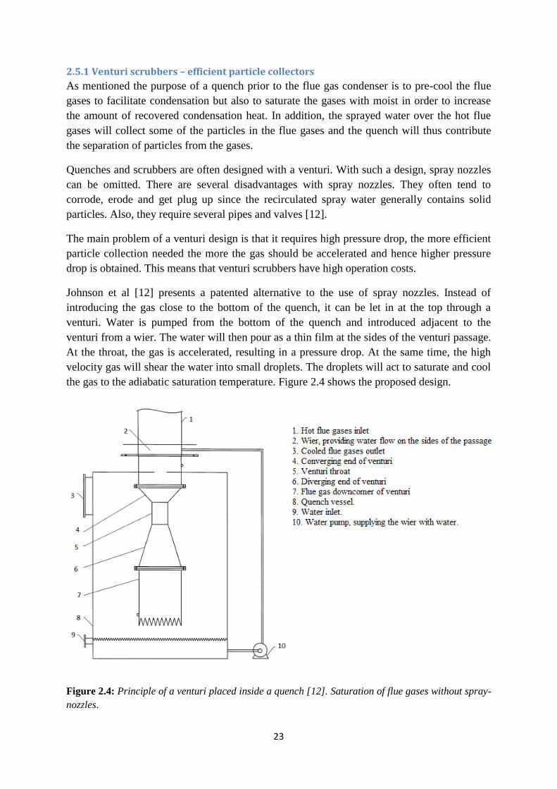
Johnson et al [12] presents a patented alternative to the use of spray nozzles. Instead of

introducing the gas close to the bottom of the quench, it can be let in at the top through a

venturi. Water is pumped from the bottom of the quench and introduced adjacent to the

venturi from a wier. The water will then pour as a thin film at the sides of the venturi passage.

At the throat, the gas is accelerated, resulting in a pressure drop. At the same time, the high

velocity gas will shear the water into small droplets. The droplets will act to saturate and cool

the gas to the adiabatic saturation temperature. Figure 2.4 shows the proposed design.

Figure 2.4: Principle of a venturi placed inside a quench [12]. Saturation of flue gases without spray-

nozzles.

24

2.5.2 Direct and indirect heat exchange of flue gases

The method of recovering energy from high temperature flue gases usually consist of the

condensation of the water present in them by heat exchanging the wet flue gas with a lower

temperature liquid medium.

Indirect heat exchanging configurations such as the one used in the Örtofta flue gas condenser

usually require the flue gas to be sprayed with water before being condensed in the heat

exchanger system. The heat can then be retrieved and supplied to a heating district network.

An alternative application is to use the wet flue gas in another stage to heat up water in order

to be used to heat up and humidify the combustion air before going into the boiler.

The patent of Mats O.J. Westermark [13] shows a method by which the energy of the flue

gases is recovered by cooling them under the dew point and condensing the water content

using indirect contact heat exchangers. In the shown process the energy coming from the

water condensation in the flue gas is transferred to the water in a district heating network but

also partly to a circuit in which water is being used to heat and saturate the air which will be

used in the combustion chamber.

Figure 2.5: Mats O.J. Westermark process [13]

In the presented arrangement the incoming flue gas first passes a spraying chamber where it

gets humidified, and then it gets heat exchanged with the heating network. After that it passes

through the second condensing stage where it is heat exchanged with the water working in the

humidifier. Flue gas can also be heated prior to the gas stack to avoid corrosion.

For the proper operating of this unit it must also be noted the fact that in order to prevent

concentrating impurities in the humidification water, this is continuously removed from the

humidifier through a pipe.

A direct heat exchanging assembly offers a different alternative to recover heat from high

temperature flue gases, in such configurations a liquid medium can be used counter currently

25

with the flue gas. An option would be having the flue gas contacted with a liquid medium in

two stages as shown in Dan Ben-Shmuel and Philip Zacuto invention [14].

Figure 2.6: Dan Ben-Shmuel and Philip Zacuto process [14]

The first stage (on top of the tower) would consist of a packed bed where the cooled down

flue gas meets fresh cool liquid condensing the water content and the possible evaporated

liquid medium into the gas in order to retrieve as much energy as possible from the flue gas

into the liquid medium.

Then the second stage would consist in thin film contactors between warm liquid coming

from the previous stage and the hot flue gas. This allows high heat transfer minimizing the

mass transfer (thus preventing heat loss due to vaporization of the liquid medium into the gas

stream). After this stage the hot liquid medium can be driven into a heat exchanger in order to

heat other streams such as water from a district heating network. After heat exchanging a part

of the liquid medium is pumped back to the sprayers in the top of the tower where another

fraction of the liquid is removed from the process.

Another advantage of direct contact arrangements is that it also performs scrubbing of the gas,

retrieving particles and dissolving noxious gases.

2.5.3 Membrane technology for flue gas processing

Wang et al [16] presents an advanced waste heat and water recovery technology for the

extraction of water vapor and its latent heat from flue gases using nano-porous ceramic

membranes. The technology can be integrated with boilers for heat and power production. In

the article, the technique is evaluated for a coal power plant at pilot scale. The main idea is

that hot flue gases are passed through a gas membrane. Inside the membrane pores, capillary

condensation of the water vapor takes places. Through the capillary condensation mode of

porous membranes, great selectivity is achieved since the condensed water in the pores

prevents other gaseous components like CO2, O2, NOx from passing through. In addition, a

high transport flux can be achieved. The water and the latent heat of condensation are

transferred with the flux stream to the boiler make up water and thus supplied to the steam

26

cycle. Heat taken for the evaporation of moist in the fuel is then regained and the plant

efficiency consequently increased [16]. A schematic for the process is depicted in Figure 2.7.

The technology uses patented Transport Membrane Condensers (TMC). The technique has

already been commercialized for industrial laundry applications and gas-fired package boilers.

It is however believed to be particularly beneficial for coal-fired plants using moist fuels

and/or flue gas desulfurization (FGD) for the cleaning of flue gases. It should be noted that

the sulfur content in flue gases from wood combustion is small. Applied to industrial steam

boilers, the TMC technology has proven to be able to recover up to 40 % of exhaust water

vapor and to increase the overall efficiency with up to five percent [16].

Figure 2.7: Schematic of the TMC concept [16]

Sijbesma et al [17] explores the possibility of removing water from flue gases using

polymeric membranes through experiments and simulations. A problem with flue gas

treatment is that the gases are cooled down and thus saturated with water before entering the

stack, which can cause condensation problems. Therefore, flue gases are typically reheated

before leaving through the stack. This can be a rather energy consuming process. Through the

dehydration of flue gases with membranes, the reheating becomes redundant. In addition,

clean water can be derived which can be reused. Membrane technology is attractive for flue

gas dehydration since it is energy efficient, reliable and leaves a small footprint. In addition,

an advantage with membrane dehydration over flue gas condensation in a gas condenser is

that there are corrosive substances in the flue gases (for example sulfur) which can damage

the condenser. This is a problem for coal fired boilers but perhaps not as much for wood fired

27

boilers due to the less corrosive nature of the flue gases. Finally, there is a possibility for

direct CO2 removal through the treatment of flue gases with membranes [17].

2.5.4 Introducing heat pumps with a flue gas condenser unit

The temperature of the return district heat flow determines how much water that will

condense in the flue gas condenser. With a high temperature the effect of a flue gas condenser

will drastically drop. For a lot of plants this means that a flue gas condenser is not profitable

enough.

In order to lower the temperature in the flue gas condenser the return district heat flow needs

to go through an installed heat pump. There are three options to implement a heat pump with

a flue gas condenser. The first option (figure 2.8) is to divide the return district heat flow into

two flows, one flow that goes though the evaporator of the heat pump and one that goes

through its condenser. The second option is to also divide the district heat flow into two

flows, but instead of letting it to pass the heat pump evaporator, it passes the top of the flue

gas condenser. The energy in the evaporator comes from a closed system between the

evaporator and the lower part of the flue gas condenser. The third option is to make the

district heat flow pass the heat pump condenser, in which the heat pump is connected with the

flue gas condenser within a closed system. The first option is considered to be the most

efficient for plants with an already installed flue gas condenser.

There are three types of heat pumps that could be applied to the system; an electric powered

heat pump, a steam driven heat pump or a steam driven adsorption heat pump. All types give

approximately the same increase in flue gas condenser effect. The electric powered heat pump

is the only alternative for plants without a steam cycle. For plants with a steam cycle all the

alternatives are possible. The decision to make is whether the plant should specialize in

electricity or heat production, because the steam powered adsorption heat pump requires

significantly more steam from the steam cycle than the steam powered heat pump.

The advantage with implementing a heat pump to a flue gas condenser is that the total

efficiency increases at least five percentage units, due to the increasing amount of condensing

water in the flue gas condenser.

The disadvantage with implementing a heat pump is that the heat pump is powered by steam

or electricity which lowers the plants electricity production. Another disadvantage is that the

temperature of the return district heating flow most be above 50°C too get a sufficient

efficiency gain in the flue gas condenser, in order for the heat pump to become cost-efficient.

[18]

28

Figure 2.8: An example of a flue gas condenser combined with a heat pump [18].

29

Part III - Calculations In this chapter the basic calculations and estimations for both Örtofta and Lomma power plant

will be presented. All equations and data constants is taken from “Data och Diagram” by

Sten-Erik Mörtstedt and Gunnar Hellsten [19] and from Örtofta which can be seen in the

appendix chapter. A process sheet is presented in appendix 9.2. The results are presented in

each chapter and also as an overall energy balance in appendix 9.3-9.8. All the calculations

are calculated with MATLAB R2012a©

.

3.1 Material calculations In material calculations the fuel material composition and energy will be calculated.

3.1.1 Material composition

The data for the different material composition were given from Örtofta and can be seen in

appendix 9.1. For this study two types of material was given, wood chips and demolition

wood. In the calculations the average number for each component was used. The components

that were used in the calculations were carbon, hydrogen, oxygen, nitrogen and water. With

the ashes the components adds up to 99.8% of the total material. The rest assumes not to take

an important part of the material- and energy balances.

3.1.2 Material energy calculations

To calculate the calorimetric heat value equation 3.1 is used. Equation 3.1 adds the energy

from the carbon and the hydrogen to get a total value for the fuel.

(3.1)

Because the fuel contains and produces water the calorimetric heat value doesn’t give the

correct result. To take into account the total amount of water, equation 3.2 were used to

calculate the effective heat value.

(3.2)

To calculate the fuel flow to the boiler equation 3.3 is used. All the results from the energy

calculations can be seen in table 3.1 below.

(3.3)

Table 3.1: The table shows the calorimetric heat value, effective heat

value and the amount of fuel needed for each case.

HS (MJ/kg) Hi (MJ/kg) fuel (kg/s)

Örtofta composition 14.7 10.7 11.2

Lomma case 1 13.6 9.69 1.83

Lomma case 2 15.1 11.1 1.60

Lomma case 3 16.6 12.5 1.42

30

3.2 Flue gas calculations In this chapter the flue gases produced by the fuel is calculated. The system boundaries for the

calculations are from the combustion to the start of the quench. The cleaning steps between

the boiler and the quench will not be taking in consideration in the calculations, and the flue

gas will be assumed to have approximately the same composition after the boiler as in to the

quench.

3.2.1 Flue gas composition calculations

The total amount of flue gas produced by the fuel is calculated with equation 3.4. In equation

3.4 each substance fraction is multiplied with a substance constant and then summed to a total

volume flue gas for 1 kg of fuel. For the amount of dry flue gas the same equation can be

applied by using a dry constant for the hydrogen and disregard the moist fraction. Equation

3.4 can also be used to calculate the amount of dry air needed in the boiler. The only

substances necessary for the air calculations are carbon, hydrogen and oxygen with

corresponding air constant.

(3.4)

To calculate the excess air flow needed in the boiler the requirement of oxygen content in the

dry flue gases is important, see equation 3.5. The dry air is assumed to contain 21% oxygen.

In table 3.2 below the different volumes for each substance is presented. The table likewise

presents the total volume for the flue gas.

(3.5)

The flue gas is assumed to only contain carbon dioxide, nitrogen, oxygen and water. From the

flue gas produced by carbon 20.95% is carbon dioxide and the rest is nitrogen. From the

combustion of hydrogen 23.61% becomes water and the rest is also nitrogen. In the excess air

21% consists of oxygen and 79% nitrogen. g0 and L0t,excess added together makes up the total

flue gas flow (g).

Table 3.2: The table shows the volume flue gas in Nm3/s for each component

produced per second and the total volume of flue gas produced both dry and wet.

CO2 O2 N2 H2O g gt

Örtofta compilation 6.82 1.68 11.6 5.00 52.5 42.1

Lomma case 1 1.03 0.365 5.49 0.773 8.65 6.88

Lomma case 2 0.996 0.353 5.10 0.749 8.13 6.67

Lomma case 3 0.968 0.234 5.19 0.78 7.74 6.50

31

3.2.2 Flue gas energy calculations

To calculate the enthalpy of the flue gas entering the quench equation 3.6 are used.

(3.6)

The flue gas enthalpy doesn’t take in consideration that the water vapor holds vaporization

energy. The vaporization energy shouldn’t be considered until the condenser. Therefore the

enthalpy given by equation 3.6 is the energy quantity that’s accessible to the quench.

3.3 Quench basic calculations In this part of the project important parameters for the quench is calculated. The optimizing of

the quench is presented in chapter 4.1.

3.3.1 Quench temperature

It’s assumed that the flue gas in the quench gets fully saturated. To get the flue gas fully

saturated the energy in the flue gas need to be sufficient to evaporate enough water. To

evaporate enough water, flue gas need to transfer energy, thereby lowering the temperature

and lowering the highest possible partial pressure of water in the flue gases, as seen in

equation 3.7 also called Antoine’s equation.

(3.7)

The highest possible amount of water the flue gases can hold can be calculated with equation

8. The partial pressure in equation 3.7 is given in Pascal and in equation 3.8 the partial

pressure is given in partial pressure/total pressure.

(3.8)

The temperature in the quench is calculated with equation 3.9. The left hand side describes the

energy needed to evaporate the added quench water. The right hand side describes the energy

given by the flue gases.

(3.9)

The temperature for each case and Örtofta is between 61°C and 65°C. To design the quench

for each case the gas flow is the only variable needed and is in table 3.2.

32

3.4 Condenser basic calculations For the calculations of the condenser the important numbers are the area, k-value and the

energy transferred to the district heating network. In this chapter these numbers will be

presented and in chapter 4.2 the numbers are used to design the condenser.

3.4.1 Condenser energy balance

To calculate the total energy output from the condenser equation 3.10 is used. First the energy

from the flue gas including water vapor is calculated from the temperature of the quench to

the outgoing temperature from the condenser. Afterwards some of the water vapor in the flue

gas will condense at the outgoing temperature and thereby achieving most part of the energy.

The amount of water vapor that not will condense is calculated with help of equation 3.7. In

reality the water vapor in the condenser will start condensing at the start, but to simplify the

calculations the condensing water vapor is calculated at the lower temperature.

(3.10)

The energy given from equation 3.10 is used in equation 3.11 to calculate the temperature of

the outgoing district heat.

(3.11)

With all the ingoing and outgoing temperatures to the condenser the logarithmic temperature

is calculated with equation 3.12.

(3.12)

To get a proper economic evaluation of the condenser the same k-value as the one in Örtofta

is applied to all cases in Lomma. The area of the condenser in Örtofta is set to 5500 2, which

means that equation 3.13 can calculate the average k-value for all condensers. All the values

for each case are presented in Table 3.3.

(3.13)

Table 3.3: The table shows the results of the condenser calculations.

A (m2)2) k (kW/ m

2)2K) Q (kW) ΔTln (ᵒC)

Örtofta 5500 0.576 17800 5.62

Lomma case 1 872 0.576 2880 5.73

Lomma case 2 712 0.576 2280 5.57

Lomma case 3 595 0.576 1840 5.35

33

3.5 Condensate water calculations The condensate flow from the condenser needs to be cleaned before let out to the

environment. The design for water treatment will be presented and discussed in Part V. This

chapter will present the calculations from the condenser to the first membrane and the water

needed to be provided the quench.

3.5.1 Condensate flow

The condensate flow from the condenser is calculated with equation 3.14. In order to get the

right unit (kg/s) the constant 1.265 converts from Nm3 to kg.

(3.14)

3.5.2 Quench flow

To calculate the quench water flow a small part of equation 3.9 is used to create equation

3.15. The required amount of water needed for saturation in the quench, , can be

derived as the difference between the amount of water which the gases holds at saturation and

the amount which enters with the flue gases going in to the quench. This amount can be

converted into a liquid mass flow (kg/s) according to equation 3.15.

(3.15)

The results from each case can be seen in Table 3.4 together with the condensate temperature.

Table 3.4: The table shows the condensate flow, the minimum

needed quench flow and the temperature of the condensate.

(kg/s) Tcond (ᵒC)

Örtofta 7.01 2.67 47

Lomma case 1 1.12 0.336 46

Lomma case 2 0.892 0.325 46

Lomma case 3 0.716 0.316 46

34

Part IV - Designing the Flue Gas Condenser Unit

for Lomma Power Plant As described in section 1.2, the flue gases coming from the flue gas cleaning unit at the

Örtofta plant are cooled and saturated with water in a quench. The quench consists of a

cylindrical vessel, with a conical bottom for particle collection. The vessel is 10 m high

except for the conical part, which accounts for an additional 4 m. The diameter of the vessel is

5.5 m. The vessel is coated with glass-fiber reinforced plastic, which is common for a quench

or a scrubber [20]. In the existing design, reject water from the water cleaning unit are

introduced at three levels in the tower through spraying nozzles. The cooling water will thus

meet the gas flow in a counter-current direction. In addition, some water is also sprayed over

the gas just prior to the quench gas inlet. A picture of the principle for the quench design is

given in Figure 4.1 (not to scale).

Figure 4.1: Principle of the quench at Örtofta to be implemented at the Lomma plant.

It has been pointed out that the main purpose of cooling the flue gases and saturating them

with water is to facilitate the condensation in the condenser, increasing the amount of

acquired latent heat delivered to the district heating network. But the quench will also help

removing particulate matter from the flue gases, which will partly be transported to the

bottom of the quench along with the formed liquid film on the inside walls of the vessel. The

particles are then transported as sludge back to the boiler and burnt. Still, most small particles

are separated in the efficient gas cleaning unit before reaching the quench.

Since the plant of Lomma has an efficient flue gas cleaning system, the problem of clogged

spray nozzles may be negligible. Also, wood-fired boilers produce less corrosive flue gases

than does e.g. coal fired boilers. Therefore, traditional spray-nozzles can be acceptable, and

35

the nozzle-free venturi design described in section 2.5.1 can be omitted. The flue gas cleaning

technique used is fabric bag house filters. Moreover, there is a flue gas desulfurization unit

(FGD) in place (see section 2.6 for further description).

4.1 Quench dimensions

The most straight forward way of constructing the quench at the Lomma plant would be to

use the same quench design as for the Örtofta plant but at a scale proportional to the smaller

flow rate of flue gases. In order to be sure to reach saturation, the gas residence time, and the

gas velocity should be the same for the two plants. Intuitively, this means that the two vessels

should have an equal height. Consequently, the cross-section area, of the vessel should be

adapted for the smaller gas flow rate. The gas velocity at Örtofta can be calculated as:

(4.1)

Where is the mean flue gas flow rate (including excess air) through the quench,

expressed as real cubic meters per second . Assuming atmospheric pressure in the

quench, can be calculated as

(4.2)

where is the flue gas flow rate, including moist and excess air, expressed as normal cubic

meters per second Since the temperature of the gases in the quench are cooled

throughout the quench, from the bottom to the top, a mean gas temperature, is used to get the

mean gas flow rate. The flow rate expressed as real cubic meters will decrease as the gases are

cooled off to the adiabatic saturation temperature, . The actual gas velocity will

consequently also decrease as the gases travels up through the quench. The mean quench

temperature is approximated as the mean value between the temperature of the entering flue

gases and the adiabatic saturation temperature, which is the temperature of the gases as they

leave the quench.

(4.3)

The quench cross-sectional area of the quench can be calculated as:

(4.4)

This means that the diameter at the Lomma plant can be calculated as:

(4.5)

(4.6)

The gas flow rate, G, for the three fuel composition cases analyzed at the Lomma plant and

the one at the Örtofta plant along with quench design parameters are given in Table 4.1.

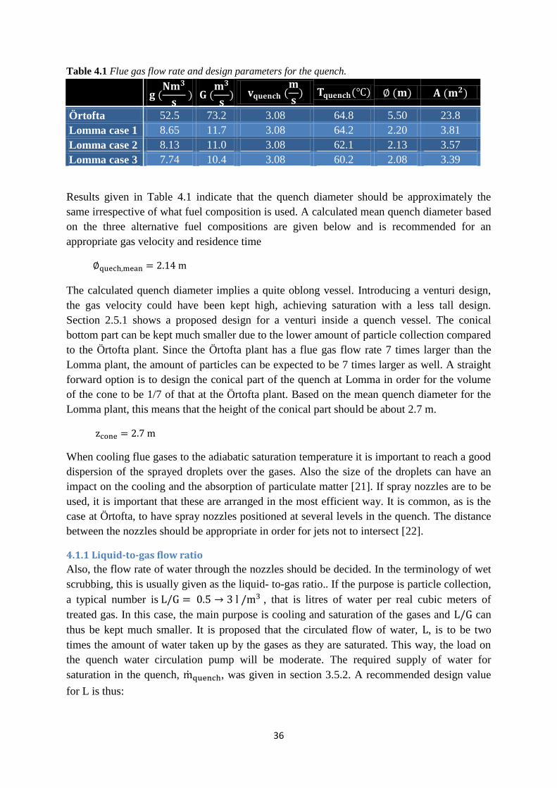
36

Table 4.1 Flue gas flow rate and design parameters for the quench.

Örtofta 52.5 73.2 3.08 64.8 5.50 23.8

Lomma case 1 8.65 11.7 3.08 64.2 2.20 3.81

Lomma case 2 8.13 11.0 3.08 62.1 2.13 3.57

Lomma case 3 7.74 10.4 3.08 60.2 2.08 3.39

Results given in Table 4.1 indicate that the quench diameter should be approximately the

same irrespective of what fuel composition is used. A calculated mean quench diameter based

on the three alternative fuel compositions are given below and is recommended for an

appropriate gas velocity and residence time

The calculated quench diameter implies a quite oblong vessel. Introducing a venturi design,

the gas velocity could have been kept high, achieving saturation with a less tall design.

Section 2.5.1 shows a proposed design for a venturi inside a quench vessel. The conical

bottom part can be kept much smaller due to the lower amount of particle collection compared

to the Örtofta plant. Since the Örtofta plant has a flue gas flow rate 7 times larger than the

Lomma plant, the amount of particles can be expected to be 7 times larger as well. A straight

forward option is to design the conical part of the quench at Lomma in order for the volume

of the cone to be 1/7 of that at the Örtofta plant. Based on the mean quench diameter for the

Lomma plant, this means that the height of the conical part should be about 2.7 m.

When cooling flue gases to the adiabatic saturation temperature it is important to reach a good

dispersion of the sprayed droplets over the gases. Also the size of the droplets can have an

impact on the cooling and the absorption of particulate matter [21]. If spray nozzles are to be

used, it is important that these are arranged in the most efficient way. It is common, as is the

case at Örtofta, to have spray nozzles positioned at several levels in the quench. The distance

between the nozzles should be appropriate in order for jets not to intersect [22].

4.1.1 Liquid-to-gas flow ratio

Also, the flow rate of water through the nozzles should be decided. In the terminology of wet

scrubbing, this is usually given as the liquid- to-gas ratio. If the purpose is particle collection,

a typical number is , that is litres of water per real cubic meters of

treated gas. In this case, the main purpose is cooling and saturation of the gases and can

thus be kept much smaller. It is proposed that the circulated flow of water, , is to be two

times the amount of water taken up by the gases as they are saturated. This way, the load on

the quench water circulation pump will be moderate. The required supply of water for

saturation in the quench, , was given in section 3.5.2. A recommended design value

for L is thus:

37

(4.7)

The water to the quench is assumed to be supplied at the adiabatic saturation temperature.

Table 4.2 gives values for L and the liquid-to-gas ratio, L/G.

Table 4.2: Required liquid circulation rate and liquid-to-gas ratio for the quench at Lomma.

Lomma case 1 0.336 0.981 0.686 63.3

Lomma case 2 0.325 0.982 0.661 65.5

Lomma case 3 0.316 0.983 0.644 67.4

In order to supply enough of water to the quench, a design value for L should be based on the

fuel composition of case 1, which requires the most water. Adding some margin, an

appropriate number is:

This corresponds to a -ratio of:

which is much less than ordinary ratios for wet scrubber particle collection.

4.2 Preliminary thermal design of the condenser There are three types of heat exchangers, recuperator, regenerator and evaporative. The

condenser in Örtofta and designed for Lomma is a recuperator, which means that the fluids

doing the heat exchange are on different sides of a dividing wall. The flow can be parallel,

counter current or cross-flow. The heat transfer coefficients will vary along the length of the

tube, so average values must be calculated – finding then a mean value for the overall

coefficient [5].

In this preliminary thermal design of the condenser some assumptions and simplifications

were done. To design a condenser there are several factors that must be determined. The ones

described in this section are: flow side, material, heat transfer area, number of tubes, tube

length and diameter, tube layout, number of shell and tube passes, type of exchanger, tube

pitch, number of baffles, type and size.

In the design of the condenser for Lomma the choice of shell and tube side flows was to have

the district heating water flow through the shell and the flue gas on the inside of the tubes, as

it is done in Örtofta. Commonly for condensation when applying shell-and-tube condensers is

to have condensation on the shell-side – this is however a set up that works better for mixtures

of condensable vapours only. For vertical in-tube condensation, if the pressure drop is not an

issue, this configuration can lead to higher heat-transfer coefficient than shell-side

38

condensation. The pressure drop can be estimated with the methods used for pure-component

condensation [15]. The material suggested for building the condenser is to also use acid

treated stainless steel in both shell and tubes - as it is in the condenser at Örtofta.

Vertical tubes preferred for subcooling of the condensate. If the vapour is superheated,

sensible and latent heat can be recovered. For multicomponent condensation there are

sensible-heat changes [15]. However, due to its low specific heat compared to the large latent

heat, the heat of superheat of the vapour is usually small. As in this case the vapour is not

highly superheated, its net effect can be disregarded. The use of the quench reduce the needed

area for the condenser as, by spraying the flue gas with water, the vapour is cooled and can be

condensed directly without needing to be de-superheated [6].

Material and energy balances are used to calculate the required heat transfer rate; and with the

overall coefficient and the temperature variation, the required area is found. The energy

balance of the condenser was done using equation 3.10, 3.11 and 3.13. The areas needed for

the heat transfer were calculated in section 3.4, based on the average k-value calculated with

the known area of the condenser at Örtofta. To have a security margin in the design, these

calculated areas were increased in 5%. As the standard sizes of tubes and equipment are given

in feet and inches, the increased areas were converted to square feet and rounded up. These

values can be seen in Table 4.3.

The tube outside diameter OD is chosen to be 25.4 mm (1 in), the tube thickness should be

chosen so that it withstands internal pressure and corrosion. The use of longer tube lengths

can reduce the diameter of the shell, but it can also lead to higher pressure drop in the shell

side. For this reason, a tube length of 6.096m (20ft) is suggested. The number of tubes needed

to achieve the calculated heat exchange area can be calculated with equation 4.8:

(4.8)

Table 4.3 Rounded up areas in square meters and in square feet and number of

tubes needed.

A (m2)

2) A (ft

2) 2K) nt

Lomma case 1 916 9900 1892

Lomma case 2 748 8100 1548

Lomma case 3 524 6800 1300

There are many possible configurations for shell-and-tube heat exchangers. A single pass 1-1

heat exchanger is more economical for requiring less metal. But the coefficients must be large

on both sides, and it is interesting to have high velocity and turbulence, also on both sides

(addition of baffles on the shell side can help to achieve this). The tubes can be placed in a

triangular or square distribution. The first is harder to clean but has a higher heat transfer area,

while the latter has lower shell-side pressure drop. This single pass configuration, however,

can suffer from vibration problems due to the high velocity flows [6].

39

The condenser type of a fixed-tube-sheet (tube sheets are welded to the shell [15]) with one

tube side and one shell side pass in counter-flow (a greater range of temperature is possible

and the required area needed is less for this configuration [5]) so it is reasonable to propose

such model for the condenser at Lomma. The tubes should fill the shell so that the maximum

number possible of tubes are fitted in there, with the tube walls having a close fit to the tube

bundle as possible. The distance between the outer layer of tubes and the inside diameter of

the shell is of 13 mm (½ in) for shells with more than 635 mm (25 in) diameters [15].

In order to have a better heat transfer, better use of area and increased turbulence, the tubes

can be placed in a triangular pattern with the tube pitch (distance between tubes from centre to

centre) of 1.25 times the outside diameter of the tubes. The suggested distribution of the tubes

is with a central tube and adding tubes in surrounding hexagons, as illustrated in Figure 4.2.

To supply the needed number of tubes for case 1 a shell with 2.01 m (79 in) in diameter is

needed, for case 2 a shell diameter of 1.85m (73 in) and for case 3 a shell diameter of 1.7 m

(67 in). In this diameter size the needed distance between the tube bundle and the shell wall is

already included. As the diameter differences for all the cases are small, it is of interest to

make a condenser with 2.0 m of diameter. This way, it will be adequate for all the cases and

have some extra tubes as a security margin, compensating for simplifications and

approximations done in the calculations and design.

Condenser Shell

Tube

Tube pitch

Figure 4.2 Tube layout in the condenser and tube pitch.

The condenser can be a baffled or an un-baffled shell-and-tube condenser. The presence of

baffles helps in stabilizing the tubes and reducing vibration problems [15]. The minimal

distance between baffles is usually of one fifth of Ds (inside diameter of the shell).

Positioning the baffles closer increases the turbulence and the heat transfer coefficient, but

40

gives a higher pressure-drop. The maximal baffle spacing is determined so that the tubes are

properly supported, the maximal tube span that can be unsupported is given by 74∙do0.75

(in

inches) [15]. In this case, with the tube diameter as 1 in, the maximal tube unsupported length

is of 74 in. For the chosen tube length of 6.09 m (20ft), this means that at least 4 baffles will

be needed. A commonly used baffle is the one with a segmental cut – a 20% cut leads to a

good heat transfer with acceptable pressure drop. If the condensation was on the shell side, it

would be interesting to have the maximum cut (45%), and use this calculated maximum

spacing in order to minimize the pressure drop [15].

41

Part V - Design for the Treatment of Condensate

Water at the Lomma Plant As previously stated, the flue gas condensate from a wood-fired power boiler plant typically

needs to be cleaned before let to any watercourse, despite efficient flue gas cleaning steps. Of

course, the demands for water purity depend on the properties of the recipient. At the power

plant of Örtofta, excess condensate is let out to the Kävlinge river after treatment. The power

plant at Lomma is close to the Höje river, which is an appropriate recipient for treated

condensate. When letting treated water to these rivers, it is of course important that neither the

aquatic life is disturbed nor the attractiveness of the water diminished. At the Örtofta plant

today, the condensate is treated with a series of membrane units with different degrees of

particle and salt retardations before being let to the recipient.

At the Örtofta plant, the condensate is partly used as make-up water for the steam cycle and

also for the district heating network. Because the condensate from the flue gas condenser is

warm, , the use of condensate for this purpose implies significant energy savings

compared to only relying on softened city water which enters at a lower temperature (also see

section 2.7). From the condenser energy balance and calculations (section 3.4 and 3.5) it was

made clear that the flue gas condensate at the Lomma plant will be almost as warm, . It

should however be remembered that the condensate temperature can be higher, up to 60

due to operational regularities.

In this section, a proposed design for the use of condensate for make-up water production is

presented, in which the present water treatment plant is utilized. In the same manner as

before, the design for condensate pre-treatment will be based on the present design at Örtofta,

which uses a combination of micro- and ultrafiltration.

5.1 Make-up water production at Lomma today Figure 9.1 in appendix shows a process flow-sheet for the current water treatment plant at

Lomma. In this setup, softened city water is treated to be used for the production of make-up

water for the steam cycle but also for the district heating network. For that purpose, the city

water is first driven through a series of reverse osmosis membranes. After these, the water

stream goes through a mixed bed in order to retain ions that have not been separated. Having

passed the mixed bed, the water goes to a tank from which it will be used either as make-up

water for the boiler or for the district heating network. In order to know how to adapt the

current design for the treatment of flue gas condensate, the next section will describe the

condensate treatment at the Örtofta plant.

42

5.2 Treatment of condensate for make-up water production at Örtofta As can be seen from the process flow-sheet for the condensate treatment and make-up water

production at the Örtofta plant, Appendix 9.9, the production of make-up water is performed

in a similar manner as for the Lomma plant. The Örtofta plant also use city water for the

production of make-up water. However, the city water is partly mixed with pre-filtered

condensate before going through the various steps of revered osmosis.

Before the condensate can be treated by the reverse osmosis steps, it needs to be pre-treated.

At Örtofta, this is done through a combination of micro- and ultrafiltration units, (MF/UF).

This is a very efficient treatment method which guarantees good water quality to the RO-units

more or less independently of the quality of the raw condensate. It is however one of the most

expensive alternatives to reversed osmosis pre-treatment [10]. As can be seen from Appendix

9.10, the flue gas condensate is first passed through the coarser MF step to get rid of smaller

particles. The reject water stream of this step is sent to the quench where it used to saturate the

flue gases.

In the next step, sodium hydroxide is added to increase the pH-level. An adapted pH-level is

important for the function and longevity of the membranes. The RO retention of salts is

significantly higher for neutral condensate compared to acidic. Also, the higher pH can

enhance the precipitation of heavy metals in the condensate in order for these to be separated

by the ultrafiltration membrane [8].

The condensate stream is then heat exchanged with the colder stream of cleaned make-up

water from the mixed bed and subsequently further cooled wither other process cooling. The

reason for additional process cooling is that only the more expensive UF- and RO-membranes

can withstand higher temperatures. The condensate normally has a temperature of after

the two stage cooling, which is a temperature that standard UF and RO-membranes can

handle [9]. This UF feed temperature can however be as high as 37 . The reject from the UF

membrane unit also goes to the quench whereas the permeate goes to the feed tank before

being further cleaned into make-up water.

At Örtofta, there is also an electrodeionization unit, EDI, with a preceding -removing step

before the mixed bed. EDI units are often coupled as tertiary treatment units to reversed

osmosis, producing ultra-clean water with conductivities below . The -

removing step is important since carbon dioxide in its dissolved form will put an unnecessary

load on the EDI, which could cause it to perform less well. However, it has been proved that

RO-systems can produce water with conductivities less than as well, which is why

it can be omitted at the Lomma plant [23].

43

5.2 Proposed design for the condensate water treatment at Lomma Power Plant

The proposed design for the condensate treatment is described in Appendix 9.11. The setup is

very much based on that used at Örtofta. It includes the MF and UF steps for pre-filtration of

macro-molecules and colloids, the addition of NaOH and exchanger for heat between the UF-

feed water and the treated make-up water. An RO-feed tank is introduced which can receive

both city water and pre-treated condensate.

A concern in implementing the membrane pre-treatment of condensate at the Lomma plant is

the quality of the permeate from the UF-filtration. If the permeate quality is worse than that of

the softened city water, there will be an increased load on the RO-membranes when

substituting city water for condensate. A higher ionic concentration in the RO feed water

means that more membrane surface area might be needed to separate the ions. It is known that

the conductivity of the raw condensate at the Örtofta plant is , supposedly at the

standard reference temperature of . The quality of the city water is which

means that the city water has a somewhat lower ionic concentration.

Sometimes, there is room for additional membranes in the existing module housing. If not,

additional modules are needed, implying even higher costs. Another main factor to take into

consideration is the power capacity of the feed pump which must be able to maintain the

pressure drop for the increased amount of membranes.

Appendix 9.11 highlights the possible position of an extra RO-membrane module, before the

RO-feed tank and the existing make-up water production plant (Appendix 9.9). This RO-unit

will work as a polish step, decreasing the concentration of salts to approximately the same

level as the softened city water. Since the condensate flow is much larger than then the

original intake of city water, it is proposed that the condensate should substitute for the city

water completely. That way, city water will only have to be brought in when the treatment of

condensate is not in operation, for example during cleaning of the membranes.

Another concern is the flow rate of condensate to the RO treatment facility. Since the flow

rate of condensate is significantly larger than the original intake of city water used for make-

up water production, the existing RO-facility will not be able to treat all the condensate, even

though the intake of city water is completely terminated and some condensate sent back to the

quench. In order to solve for this problem, some of the pre-treated water is sent to the

recipient after the extra RO-unit and not to the RO-feed tank. This water will have

conductivity as low as city water, which implies salt concentrations corresponding to fresh

water. Actually, plants are obliged to pass flue gas condensate through at least one step of

reversed osmosis. Also, this water will have reduced concentrations of sulfur, heavy metals

and COD due to the MF/UF pre-filtration steps.

The quantity of pre-treated condensate send to the RO-feed tank should equal the amount of

city water previously received to the treatment plant and everything else should be send to the

recipient. This way, no changes will have to be made to the existing treatment plant for make-

up water production, since it will receive treated condensate of the same quality and quantity

as it is currently receiving city water.

44

5.2.1 Design calculations for the pre-treatment of condensate at Lomma

Design calculations for the pre-treatment of condensate where performed by solving a system

of equations with Matlab. Used variables are depicted in the flow sheet presented in Figure

9.3. The flow rates of condensate to the membranes and retentate to the quench was calculated

from the corresponding mass flows, table 3.4, assuming an average water density. In the water

pre-treatment plant, the temperature varies between 30 and 46 . For simplicity, the density

used for all flow conversions was therefore .

It is assumed that the concentration of salts in the feed water to the extra RO-stage will be the

same as for the raw condensate from the condenser. This is because MF and UF membranes

typically do not retard any dissolved salts. Also, the addition of NaOH for bringing the

solution at a neutral or slightly alkaline level of pH corresponds to a negligible increase of the

salt concentration. RO-membranes are characterized by high retention of conductivity. A

typical number i at a neutral pH. [10]. However, condensate is harder to treat than

for example city water. At Örtofta, retentions between 75 – 85% have been observed.

Therefore, the retention, , was set to 75 % in this case. From equation 2.12, it is known

that the conductivity of the permeate from the extra RO-unit can be calculated according to

equation 5.1.

(5.1)

Since the raw condensate has a conductivity of about , permeate from this unit,

that is the feed water to the RO-tank and the RO-permeate led to the recipient, will have a

conductivity of . As stated previously, this corresponds to city water quality and

should not harm the recipient.

The permeate flow rates from the MF, UF and the extra RO-unit can be expressed according

to equation 5.2-4.

(5.2)

(5.3)

(5.4)

The feed water to the tank equals the extra RO-unit permeate subtracted by the bypassed

water going to the recipient, equation 5.5.

(5.5)

In order to adapt for the supply of water to the quench, constituted by the retentate streams of

the pre-filtration units, the volume reductions for each of these units must be decided. It

should be possible to use the retentate streams of existing RO-units for this purpose, but since

the operation conditions of these are unknown that option was omitted. The volume reduction

of RO-units is typically in the range of . For calculations, the volume reduction of

the extra RO-unit was set to 85%. The volume reductions of the MF and the UF units were

then adapted so as to meet the demand for quench water exactly. To simplify calculations, the

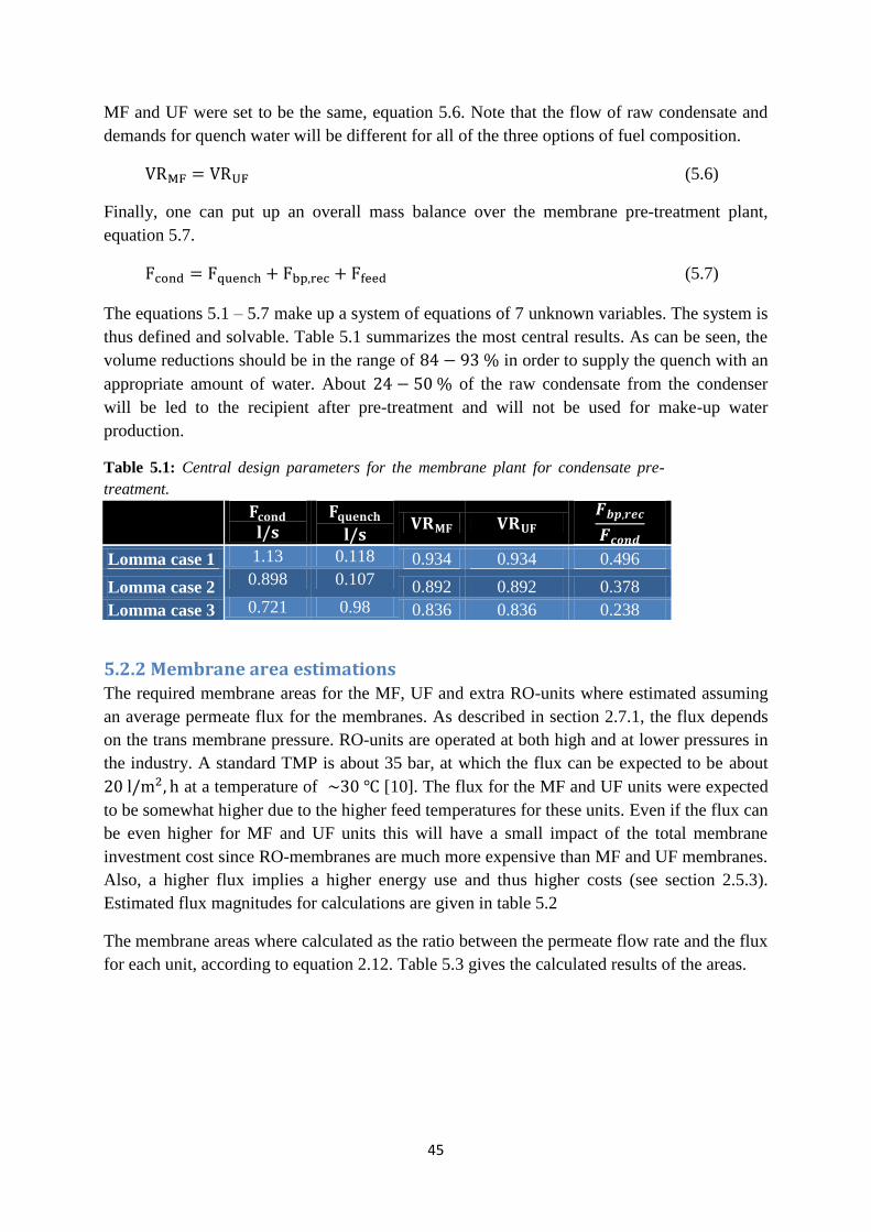
45

MF and UF were set to be the same, equation 5.6. Note that the flow of raw condensate and

demands for quench water will be different for all of the three options of fuel composition.

(5.6)

Finally, one can put up an overall mass balance over the membrane pre-treatment plant,

equation 5.7.

(5.7)

The equations 5.1 – 5.7 make up a system of equations of 7 unknown variables. The system is

thus defined and solvable. Table 5.1 summarizes the most central results. As can be seen, the

volume reductions should be in the range of in order to supply the quench with an

appropriate amount of water. About of the raw condensate from the condenser

will be led to the recipient after pre-treatment and will not be used for make-up water

production.

Table 5.1: Central design parameters for the membrane plant for condensate pre-

treatment.

l/s

l/s

Lomma case 1 1.13 0.118 0.934 0.934 0.496

Lomma case 2 0.898 0.107 0.892 0.892 0.378

Lomma case 3 0.721 0.98 0.836 0.836 0.238

5.2.2 Membrane area estimations The required membrane areas for the MF, UF and extra RO-units where estimated assuming

an average permeate flux for the membranes. As described in section 2.7.1, the flux depends

on the trans membrane pressure. RO-units are operated at both high and at lower pressures in

the industry. A standard TMP is about 35 bar, at which the flux can be expected to be about

at a temperature of [10]. The flux for the MF and UF units were expected

to be somewhat higher due to the higher feed temperatures for these units. Even if the flux can

be even higher for MF and UF units this will have a small impact of the total membrane

investment cost since RO-membranes are much more expensive than MF and UF membranes.

Also, a higher flux implies a higher energy use and thus higher costs (see section 2.5.3).

Estimated flux magnitudes for calculations are given in table 5.2

The membrane areas where calculated as the ratio between the permeate flow rate and the flux

for each unit, according to equation 2.12. Table 5.3 gives the calculated results of the areas.

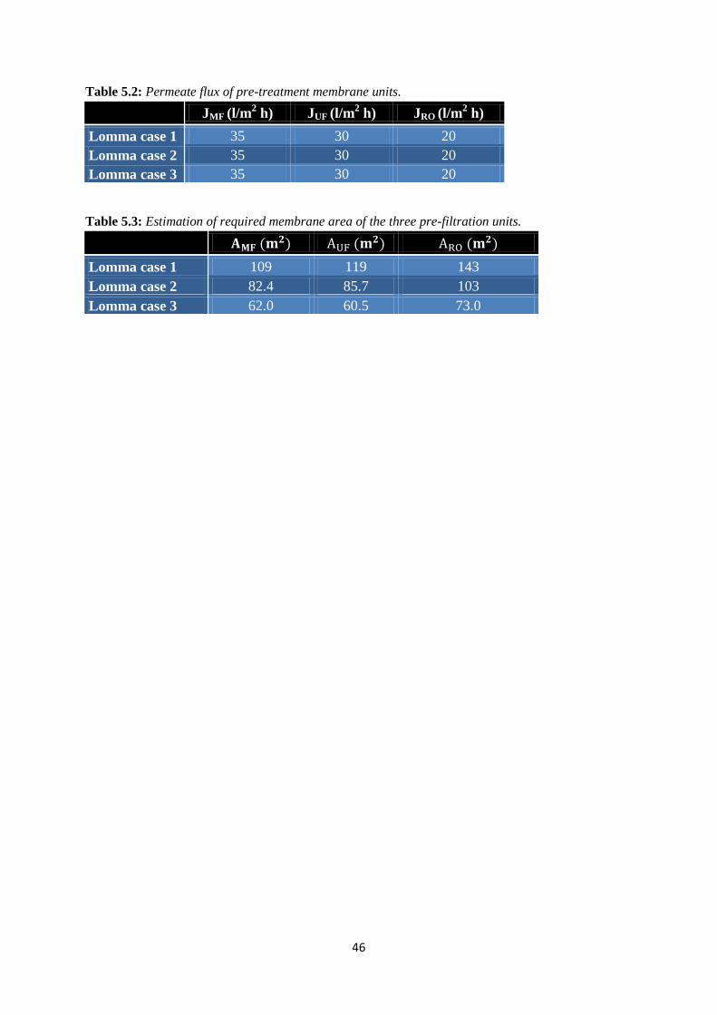
46

Table 5.2: Permeate flux of pre-treatment membrane units.

JMF (l/m2 h) JUF (l/m

2 h) JRO (l/m

2 h)

Lomma case 1 35 30 20

Lomma case 2 35 30 20

Lomma case 3 35 30 20

Table 5.3: Estimation of required membrane area of the three pre-filtration units.

Lomma case 1 109 119 143

Lomma case 2 82.4 85.7 103

Lomma case 3 62.0 60.5 73.0

47

Part VI – Estimation of Costs This chapter is investigating if it’s profitable to install a flue gas condenser at Lomma

återbruk. It starts with an assessment of the investment for each case. For each case an annual

income and expense is calculated. The results is given with two methods, pay off method and

net present value method. The results are also tested with a sensitivity analysis to confirm a

secure investment.

6.1 Investment The investment cost can be divided into separate parts, each with a different way of determine

its cost. The price for each part is presented in Table 6.1 and Table 6.2. Too individually

estimate the cost of each part the Ulrich method are used. There are two versions of Ulrich

method, manual and interactive. The two different total investment costs will be compared

with Radscans offer on 15 million SEK. The version described below is Ulrich manual

method. Both Ulrich methods give total costs in American dollars and uses CE plant cost

index equal to 400. In the tables the total cost is transformed to Swedish SEK with

equation 6.1. The CE plant cost index is approximated to 565 and the currency is 7.4 SEK/$

(6.1)

6.1.1 Quench

The quench is approximated to a vertically oriented process vessel. The cost is obtained with

the height and the diameter. Together with the combined factor the total cost for the quench

can be calculated according to equation 6.2. The material used in the quench is glass fiber

which gives a material factor of 4. Because the pressure is under 2 bar the pressure factor is 1.

These two factors give a combined factor of 9.5.

(6.2)

6.1.2 Condenser

The condenser is designed as a shell and tube heat exchanger. The cost for the condenser is

acquired with the area of the tubes. The material factor of the stainless steel condenser is 3

and the pressure factor is 1. Together the combined factor becomes 6. To calculate the total

cost for the condenser equation 6.2 is used.

6.1.3 Water treatment

The water treatment is divided into three parts, micro filtration membrane (MF), ultra

filtration membrane (UF) and reverse osmosis membrane (RO). The cost for each membrane

is determined by the membrane area. The total cost for the membranes is given without any

factor but an increase in annual spare parts is needed due to expensive membrane exchanges.

48

Table 6.1: the table shows the results from Ulrich manual method for each part and

the total investment cost. (MSEK)

quench condenser MF UF RO ∑

Lomma case 1 5.46 3.76 0.732 0.732 2.09 12.8

Lomma case 2 5.46 2.82 0.679 0.627 1.67 11.3

Lomma case 3 5.46 2.51 0.470 0.418 1.36 10.2

Table 6.2: The table shows the results from Ulrich interactive method for each part

and the total investment cost. (MSEK)

quench condenser MF UF RO ∑

Lomma case 1 5.71 4.16 0.814 0.740 2.10 13.5

Lomma case 2 5.71 2.94 0.636 0.548 1.67 11.5

Lomma case 3 5.71 2.48 0.496 0.400 1.30 10.4

6.2 Income & expenses To calculate the annual income from each case equation 6.3 is used. The price for the district

heating is given by SEKaftringen AB and is 360 SEK/MWh. The operating time for Lomma

återbruk is 9.5 months/year. The power produced each year depends on each case.

(6.3)

The expense varies a lot between the cases. That’s because the fuel cost in case 1 and 2 is

higher. In case 3 the fuel is the same as before and therefore no extra expense for the fuel. The

annual cost for maintenances and repairs is assumed to be approximately 5% of the

investment. It’s assumed that the different membranes need to be exchange at an annual or

biannual rate. The cost for spare parts is therefore approximated to add 15% of the

maintenance and repair costs.

(6.4)

The annual net cash flow is calculated with equation 6.4 and is the difference between the annual

income and the annual expenses. In Table 6.3 the results from the annual income, annual expense and

the annual net cash flow is presented for each case.

Table 6.3: The table shows the annual income, annual

expense and the annual net cash flow for each case.

(MSEK/year)

Income Expense a

Lomma case 1 7.18 6.90 0.284

Lomma case 2 5.70 3.29 2.42

Lomma case 3 4.58 0.588 4.00

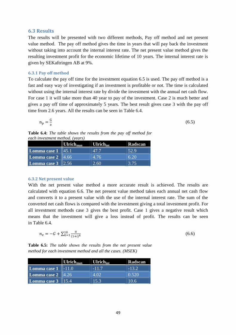
49

6.3 Results The results will be presented with two different methods, Pay off method and net present

value method. The pay off method gives the time in years that will pay back the investment

without taking into account the internal interest rate. The net present value method gives the

resulting investment profit for the economic lifetime of 10 years. The internal interest rate is

given by SEKaftringen AB at 9%.

6.3.1 Pay off method

To calculate the pay off time for the investment equation 6.5 is used. The pay off method is a

fast and easy way of investigating if an investment is profitable or not. The time is calculated

without using the internal interest rate by divide the investment with the annual net cash flow.

For case 1 it will take more than 40 year to pay of the investment. Case 2 is much better and

gives a pay off time of approximately 5 years. The best result gives case 3 with the pay off

time from 2.6 years. All the results can be seen in Table 6.4.

(6.5)

Table 6.4: The table shows the results from the pay off method for

each investment method. (years)

Ulrichman Ulrichint Radscan

Lomma case 1 45.1 47.7 52.9

Lomma case 2 4.66 4.76 6.20

Lomma case 3 2.56 2.60 3.75

6.3.2 Net present value

With the net present value method a more accurate result is achieved. The results are

calculated with equation 6.6. The net present value method takes each annual net cash flow

and converts it to a present value with the use of the internal interest rate. The sum of the

converted net cash flows is compared with the investment giving a total investment profit. For

all investment methods case 3 gives the best profit. Case 1 gives a negative result which

means that the investment will give a loss instead of profit. The results can be seen

in Table 6.4.

(6.6)

Table 6.5: The table shows the results from the net present value

method for each investment method and all the cases. (MSEK)

Ulrichman Ulrichint Radscan

Lomma case 1 -11.0 -11.7 -13.2

Lomma case 2 4.26 4.02 0.520

Lomma case 3 15.4 15.3 10.6

50

6.4 Sensitivity analysis In the sensitivity analysis the stability of the results will be tested. The two constants,

condenser outgoing temperature and price difference between the fuels, will be changed. The

sensitivity analysis calculations are based on the Ulrich manual method and will be compared

with the results from the previous chapter.

6.4.1 Condenser outgoing temperature changes

If the outgoing condenser temperature goes up the needed condenser area will be smaller

thereby lowering the investment cost. Also the condensate flow will be lower, giving less

membrane area, thus achieving a lower investment cost. But the smaller condenser area will

give a smaller energy output. The result when the outgoing condenser temperature is 50ᵒC can

be seen in Table 6.6 and 54ᵒC in Table 6.7. From the results it can be seen that case 1 is

highly sensitive to temperature rise in compare to case 3 that gives both a good result in pay

off time and in net present value for both temperatures.

Table 6.6: The table shows the change in condenser area, energy output, investment

cost, pay off result and net present value result when the outgoing temperature in the

condenser is 50°C

A (m2) Q (MW) Ginv (MSEK) np (years) nv (MSEK)

Lomma case 1 481 2.47 10.7 ∞ -14.6

Lomma case 2 377 1.89 9.48 6.18 0.369

Lomma case 3 300 1.45 8.44 2.69 11.7

Table 6.7: The table shows the change in condenser area, energy output, investment cost,

pay off result and net present value result when the outgoing temperature in the

condenser is 54°C

A (m2) Q (MW) Ginv (MSEK) np (years) nv (MSEK)

Lomma case 1 289 1.97 9.54 ∞ -21.1

Lomma case 2 212 1.41 8.00 19.0 -5.30

Lomma case 3 153 0.989 7.13 3.46 6.09

6.4.2 Fuel price changes

Lomma återbruk already uses demolition wood which means that the fuel cost is already paid

for in case 3. But for case 1 and 2 there are a difference in price per MWh. This difference can

change during the flue gas condensers life-span. The difference in price per MWh between the

fuels is 50 SEK (May-2014). The results are presented with pay off method in Table 6.8 and

with net present value in Table 6.9. The results show that case1 and 2 is sensitive to changes

in fuel prices.

51

Table 6.8: The table shows the result with the pay off method when the

change in price difference between the fuels varies. (years)

np Δp=75SEK np Δp=25SEK np Δp=0SEK

Lomma case 1 ∞ 3.80 1.98

Lomma case 2 10.4 3.00 2.21

Lomma case 3 2.56 2.56 2.56

Table 6.9: The table shows the result with the net present value method

when the change in price difference between the fuels varies. (MSEK)

nv Δp=75SEK nv Δp=25SEK nv Δp=0SEK

Lomma case 1 -30.7 8.82 28.6

Lomma case 2 -4.34 12.9 21.5

Lomma case 3 15.4 15.4 15.4

52

Part VII – Discussion & Conclusions

In this section, alternatives for the proposed design for the flue gas condenser unit and the

condensate treatment plant are presented and evaluated. Advantages and disadvantages are

presented and assumptions for design calculations discussed.

7.1 Alternative methods for the condensation of flue gases In section 2.5, several alternative methods for the condensation of hot flue gases were

presented. Here, these are evaluated and compared to the proposed design.

7.1.1 Venturi scrubbing

An alternative design for a plain cylindrical vessel for the quench design was to introduce a

venturi scrubber. With a venturi, a high gas velocity can be achieved without having to make

the quench vessel very narrow and oblong in order to adapt for the lower flue gas flow rate at

the Lomma plant. It was also mentioned that venturi scrubbers can be designed without spray

nozzles, which often get clogged up or corroded. Also, the particle collection efficiency might

be higher. Particle collection is however not the main purpose of the quench in this case, but

instead the quench is intended to saturate the flue gases with moist. In addition, the plain

quench design seemed more simple and cheaper to operate since venture scrubbers need a

high energy input to work due to the inherent pressure drop required for their operation.

7.1.2 Flue gas condensation with membranes

The use of membranes for the condensation of flue gases is an interesting alternative to the

traditional condenser design. Condensation with membranes also gives rise to a considerable

increase of the overall plant efficiency. The perhaps most apparent advantage is the separation

of gases like CO2 and NOx, reducing the emissions of these to the atmosphere. This

technology is however less proven on a commercial scale than the more traditional design for

flue gas condensation used at Örtofta.

7.1.3 Direct and indirect heat exchange of flue gases

A studied alternative method to the current arrangement of the flue gas condenser unit in

Örtofta was studied. That is the use of a direct heat exchanging assembly instead of indirect

heat exchanging. That meant that the flue gas would be in contact with a liquid medium to

retrieve heat from them. The main advantage of such an arrangement was that it also performs

scrubbing duties on the flue gas reducing particle content but it was not used since the

presence of the flue gas cleaning unit and to a lesser extent the quench already clean the flue

gas from particles to the desired levels.

7.1.4 Heat pump

Because of the low district heat incoming temperature installing a heat pump to Lomma

återbruk will not be cost efficient. It’s possible for a larger power plant like Örtofta to be able

to produce enough extra power that will make the heat pump profitable, even when the

temperature of the district heat is as low as 45°C. Lomma återbruk is therefor too small for a

53

possible installation of a heat pump when the temperature of the district heat is lower than

50°C.

7.2 Design considerations When designing for the flue gas condenser unit and the condensate treatment plant, one has to

make evaluations for the operating conditions and assumptions for the calculations. Here,

important considerations for the main steps of design are discussed.

7.2.1 Quench design

To scale the quench vessel down for the Lomma plant to adapt for the lower flow rate of flue

gases compared to the plant at Örtofta is a straight forward way to go for the quench design.

The quench dimensions should be adapted in order to reach an efficient saturation and particle

collection of the flue gases. This could be achieved by keeping the residence time and gas

velocity the same as for the Örtofta plant. If the vessel height and the flue gas velocity is kept

constant, the residence time should be the same. However, the actual gas velocity changes

with the height of the vessel. Therefore, average numbers for gas velocity had to be used. On

the whole, the dimensioning of the quench is rather approximate and the proposed design

dimensions might not be optimized for best performance. Still, the quench design calculations

give a good idea of the quench costs. Also, fuel composition and flue gas flow rates might be

changed and it is consequently hard to give optimal dimensions anyway.

7.2.2 Condenser design

Due to the complexity associated to condensers, some uncertainty is present in the designing

of the unit. The final design is a compromise that gives the best performance while still

concurring with the existing requirements and limitations. An optimal heat exchanger

balances the heat transfer area with the energy cost of pumping the fluids. There are a few

problems associated with the design, they are to reduce the pressure drop, as it can affect the

thermal efficiency; avoid the build-up of non-condensable gases that can lead to poor

performance and a reduction in the condensation rate; and the estimation of the heat transfer

coefficient of the condensate film. The issues to consider are the removal of non-condensable

gases with the addition of vents, and assuring the vapour has paths to access all the areas of

the tube-bundle.

7.2.3 Design for the treatment of condensate

The condensate from the flue gas condenser should be treated before entering the recipient in

order to avoid any substantial environmental impact. It is proposed that the water treatment is

to be done similarly to the way it is done at Örtofta, using MF- and UF pre-filtration and then

RO-membranes.

The proposed design for the pre-treatment of condensate makes it possible to use a part of the

condensate for boiler and district heating make-up water. The supply of condensate will be

large enough to substitute for the city water currently bought for this purpose. However, the

cost savings of not buying city water will be minor, only about 60 000 SEK/year for an intake

of 20 m3/day at a water price of 10 SEK/m3. The investment cost for the membranes for

condensate pre-treatment is about 2.2 – 3.5 million SEK, depending on which fuel

composition case is considered, and then there are also the costs of operation. It is thus not

54

motivated to pre-treat the condensate for make-up water production from an economical point

of view. The reason why it was proposed that condensate is to be used for make-up water

production is that this water must be pre-filtered anyway, before reaching the recipient.

Whether or not used for make-up water, the condensate should be treated with MF and UF

units to prevent ashes, tar, heavy metals and incomplete combusted organic material to enter

the recipient. The concentration of salt in the condensate corresponds to threshold levels for

fresh water. Treating the condensate that goes to the recipient with reversed osmosis is

perhaps not necessary for the protection of the river water. However, power plants are obliged

by law to treat all condensate with at least one step of reversed osmosis and this is also done

at the Örtofta plant. The extra RO-unit will bear the by far highest investment cost of the

proposed membrane units, more than three times higher than the MF and UF-units.

7.3 Case investment evaluation It’s possible to get more energy output with case 1 in compare to case 2 and 3 but that comes

with extra expenses. These expenses make case 1 highly sensitive to changes in the

production and in prices, especially if the outgoing condensate temperature becomes a few

degrees higher. The extra expenses consist mainly of the additional cost for wood chips.

Because Lomma återbruk already uses demolition wood these fuel expenses is already taken

care of with the steam cycle. That means that if Lomma återbruk instead changes to wood

chips only because of the flue gas condenser, then the extra fuel expenses should be paid with

the income from the condenser unit.

A more stable version is case 3. Case 3 uses only demolition wood as fuel which means that

no extra expense thereby stabilizing the investment. Case 3 will give a lower income because

of a lower energy output from the condenser, but with the low annual expenses case 3 gives

best results in both in the pay off method and in the net present value method. Case 3 also

shows a stable result in the sensitivity analysis making case 3 the safest investment. Case 2 is

a combination of case 1 and 3, that gives a higher energy output then case 3 and with lower

annual expenses then case 1. That means that case 2 also is more stable the case 1 and give a

higher annual income then case 3. But case 2 have a small window between the other cases

when it’s considered most profitable. That makes case 2 most profitable during precise time

intervals.

According to Table 6.4 and Table 6.5 it’s most profitable with case 3 when the investment

cost is the same for each case. This means it’s possible to design for case 1 and run the plant

with demolition wood and still be more profitable then with wood chips. That makes it

possible to change to wood chips when the conditions are such that it’s more profitable to fire

with wood chips.

55

7.4 Conclusions In order to calculate the operating conditions for Lomma, the calculations were based on the

power plant at Örtofta which already has a flue gas condensing unit operating, and were tuned

down for the smaller plant. Three different cases were considered when operating for Lomma

with three different fuel mixtures. From a cost point of view the optimal case resulted to be

case 3, using only demolition wood, and therefore the following conclusions will be referring

to that case.

A new quench and condenser were designed for the implementation at Lomma power plant.

The main idea with the quench design was to scale the quench at Örtofta in order to process

the lesser amount of flue gas but keeping the same gas velocity and residence time. Therefore

a thinner quench but with the same height was designed. The diameter of the quench was

calculated to 2.14 m.

In a similar way the condenser was designed as a tuned down version of the one in Örtofta

with less surface area which was calculated to 595 m2. This condenser would recover 1840

kW.

The present water treatment at Lomma was redesigned in order to treat the condensate coming

from the flue gas condenser unit. This part was also designed in a similar way to the one

present in Örtofta, with micro- and ultrafiltration units prior to the existing water treatment

facility but also an extra reverse osmosis step was added. The required membrane area is 62.0

m2 of microfiltration, 60.5 m

2 of ultrafiltration and 73.0 m

2 of reverse osmosis. By

implementing this design, the consumption of city water for the production of make-up water

for the boiler and the district heating network is also reduced thus reducing the total expenses.

Finally the cost of the implementation of the project was calculated and the results show that

the most profitable situation is using case 3 i.e. using only demolition wood as fuel. This

corresponds to an annual income of 4.58 million SEK, a relatively short pay off time of 2.56

years and a net present investment value of 15.4 million SEK.

56

Part VIII – References

[1] D.Che, Y. Liu, C. Gao. “Evaluation of retrofitting a conventional natural gas fired boiler

into a condensing boiler”. Energy Conversion and Management. 2004, no 45, p1051-1066.

[2]Q. Chen et al. “Condensing boilers applications in the process industry”. Applied Energy.

2012, no 89, 22-36.

[3] Gröhn, Suonmaa, Auvinen, Lethinen, Jokiniemi. ”Reduction of Fine Particle Emissions

from Wood Combustion with Optimized Condensing Heat Exchangers”. Environ. Sci.

Technol. 2009, No: 43, p.6269–6274.

[4] D. Blumberga, E. Vigants, I. Veidenbergs. ”Analysis of Flue Gas Condenser Operation”.

Lativan Journal of Physics and Technical Sciences. 2011, No 4.

[5] T. D. Eastop, A. McConkey. “Applied Thermodynamics for Engineering Technologists”.

Longman. 5th

rev. edition (1993)

[6] W. L. McCabe, J. C. Smith, P. Harriott. “Unit Operations of Chemical Engineering”.

McGraw-Hill International Edition. 7th

edition (2005)

[7] Beachler, David S. - Joseph, Jerry - Pompelia, Mick. " Fabric Filter Bag Cleaning". North

Carolina State University. 1995.

[8] Westermark, Mats. ”Flue Gas Condensation Cleaning Technology ”. Stiftelsen för

värmeteknisk forskning, (1996)

[9] Falk, Ian – Svensson, Jan. “Tillämpning av membranteknik för behandling av

processvatten vid Energiproduktionsanläggningar”. Stiftelsen för värmeteknisk forskning,

(1992)

[10] Axby, Fredrik. ”Avsaltning av varmt rökgaskondensat med membranteknik”.

Värmeforsk, (1998)

[11] Jönsson, Ann-Sofi. “Membranprocesser – grundläggande begrepp”. Inst. of Chemical

Engineering, LTH. Lund: 2014.

[12] Johnson, Bruce – Trimble, Robert - Desai, Randhir. Method and Apparatus for

Quenching Hot Flue Gases. U.S. Patent No: 6,149,137. (2000)

[13] Mats O.J. Westermark. “Method and arrangement for condensing flue gases”. U.S.

Patent 4,799,941, 24 January 1989.

[14] Dan Ben-Shmuel, Philip Zacuto “Process for recovering heat from stack or flue gas”.

U.S. Patent 4,230,572, 20 July 1982.

[15] D. W. Green, R. H. Perry, R. L. Shilling, P. M. Bernhagen, V. M. Goldschimidt, P. S.

Hrnjak, D. Johnson, K. D. Timmerhaus. “Perry’s Chemical Engineers Handbook – Heat-

Transfer Equipment”. McGraw-Hill Companies. 8th edition (2008)

57

[16] D. Wang, A. Bao, W. Kunc, W. Liss. “Coal power plant flue gas waste heat and water

recovery”. Applied Energy. 2012, No: 91, p.231–238

[17] Sijbesma et al. “Flue gas dehydration using polymer membranes”. Journal of Membrane

Science. No: 93, p.263–276, 2008.

[18] Fredrik Axby, Camilla Pettersson. ”Rökgaskondensering med värmepump”. Värmeforsk

– värmeteknisk forskning och utveckling, November 2004.

[19] Mörstedt, Sten-Erik – Hellsten, Gunnar. ”Data och diagram. Energi- och kemitekniska

tabeller”. Stockholm: Liber Ab, 2012.

[20] Ragnarsson, Sven. Method and Apparatus for Treating Flue Gas. U.S. Patent No:

6,562,83 B1. (2003)

[21] Silva, A.M. - Teixeira, J.C.F. – Teixeira, S.F.C.F. “Experiments in large scale venturi

scrubber. Part II. Droplet size”. Chemical Engineering and Processing 48, p. 424–49. (2009)

[22] Ananthanarayanan, Nochur – Viswanathan, Shekar. “Effect of Nozzle Arrangement on

Venturi Scrubber Performance”. Ind. Eng. Chem. Res. 38, 4889 – 4900. (1999)

[23] Čuda, P – Pospíšil, P – Tenglerová, J. “Reverse osmosis in water treatment for boilers”.

Desalination. 2006, no 198, 171–46.

58

Part VIII – Appendix

9.1 Fuel data sheet

59

9.2 Overall process sheet for the flue gas condenser at the power plants of

Örtofta and Lomma.

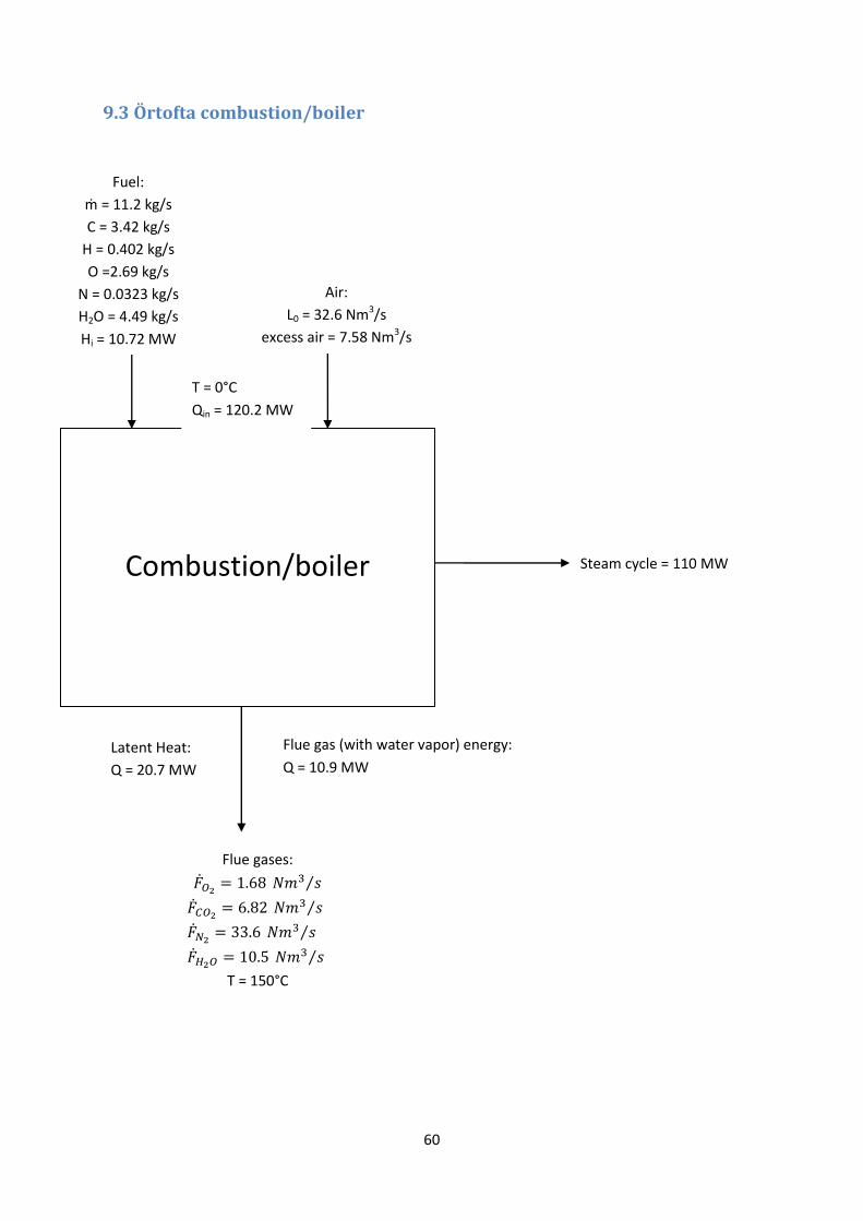
60

9.3 Örtofta combustion/boiler

Flue gases:

T = 150°C

Combustion/boiler Steam cycle = 110 MW

Fuel:

ṁ = 11.2 kg/s

C = 3.42 kg/s

H = 0.402 kg/s

O =2.69 kg/s

N = 0.0323 kg/s

H2O = 4.49 kg/s

Hi = 10.72 MW

Air:

L0 = 32.6 Nm3/s

excess air = 7.58 Nm3/s

T = 0°C

Qin = 120.2 MW

Flue gas (with water vapor) energy:

Q = 10.9 MW Latent Heat:

Q = 20.7 MW

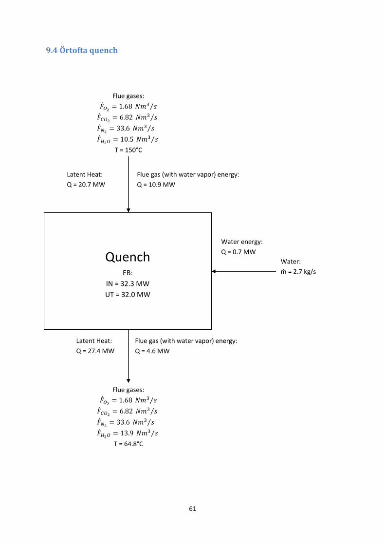
61

9.4 Örtofta quench

Flue gases:

T = 150°C

Quench EB:

IN = 32.3 MW

UT = 32.0 MW

Flue gas (with water vapor) energy:

Q = 10.9 MW

Latent Heat:

Q = 20.7 MW

Water energy:

Q = 0.7 MW

Water:

ṁ = 2.7 kg/s

Flue gas (with water vapor) energy:

Q = 4.6 MW

Latent Heat:

Q = 27.4 MW

Flue gases:

T = 64.8°C

62

9.5 Örtofta condenser

Flue gases:

T = 64.8°C

D.H.

Q = 17.8

MW

Condenser EB:

IN = 32.0 MW

UT = 32.1 MW

Flue gas (with water vapor) energy:

Q = 4.6 MW

Latent Heat:

Q = 27.4 MW

Flue gas (with water vapor)

energy:

Q = 3.0 MW

Latent Heat:

Q = 9.9 MW

Flue gas (with water vapor)

energy:

Q = 1.1 MW

Latent Heat:

Q = 16.7 MW

Flue gas:

T = 47°C

Condensate:

ṁ = 7.0 kg/s

T = 47°C

Water energy:

Q = 1.4 MW

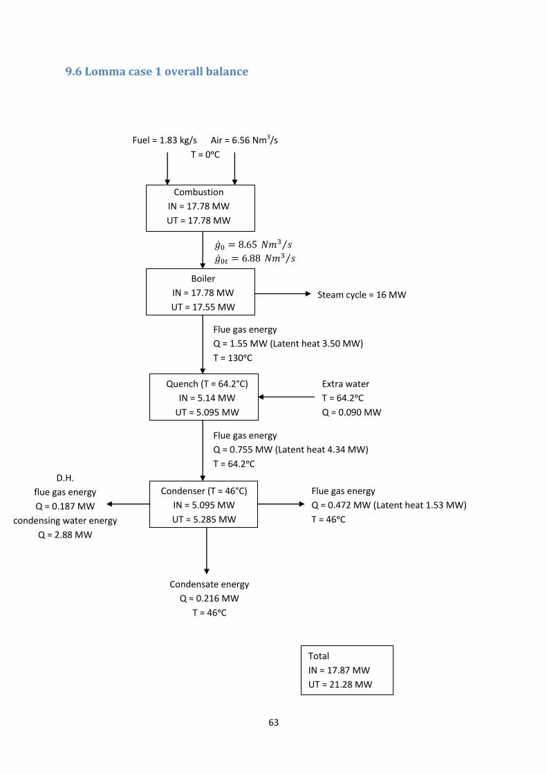
63

9.6 Lomma case 1 overall balance

D.H.

flue gas energy

Q = 0.187 MW

condensing water energy

Q = 2.88 MW

Fuel = 1.83 kg/s Air = 6.56 Nm3/s

T = 0ᵒC

Combustion

IN = 17.78 MW

UT = 17.78 MW

Boiler

IN = 17.78 MW

UT = 17.55 MW Steam cycle = 16 MW

Quench (T = 64.2°C)

IN = 5.14 MW

UT = 5.095 MW

Extra water

T = 64.2ᵒC

Q = 0.090 MW

Flue gas energy

Q = 1.55 MW (Latent heat 3.50 MW)

T = 130ᵒC

Condenser (T = 46°C)

IN = 5.095 MW

UT = 5.285 MW

Flue gas energy

Q = 0.755 MW (Latent heat 4.34 MW)

T = 64.2ᵒC

Flue gas energy

Q = 0.472 MW (Latent heat 1.53 MW)

T = 46ᵒC

Condensate energy

Q = 0.216 MW

T = 46ᵒC

Total

IN = 17.87 MW

UT = 21.28 MW

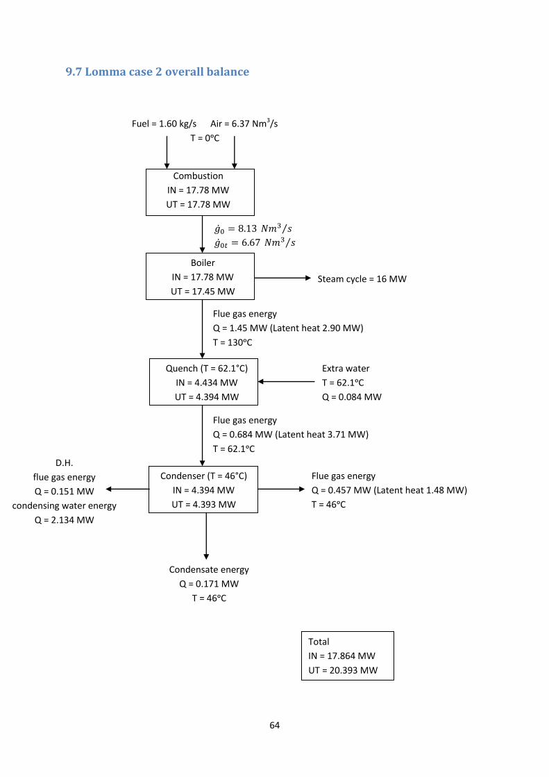
64

9.7 Lomma case 2 overall balance

D.H.

flue gas energy

Q = 0.151 MW

condensing water energy

Q = 2.134 MW

Fuel = 1.60 kg/s Air = 6.37 Nm3/s

T = 0ᵒC

Combustion

IN = 17.78 MW

UT = 17.78 MW

Boiler

IN = 17.78 MW

UT = 17.45 MW Steam cycle = 16 MW

Quench (T = 62.1°C)

IN = 4.434 MW

UT = 4.394 MW

Extra water

T = 62.1ᵒC

Q = 0.084 MW

Flue gas energy

Q = 1.45 MW (Latent heat 2.90 MW)

T = 130ᵒC

Condenser (T = 46°C)

IN = 4.394 MW

UT = 4.393 MW

Flue gas energy

Q = 0.684 MW (Latent heat 3.71 MW)

T = 62.1ᵒC

Flue gas energy

Q = 0.457 MW (Latent heat 1.48 MW)

T = 46ᵒC

Condensate energy

Q = 0.171 MW

T = 46ᵒC

Total

IN = 17.864 MW

UT = 20.393 MW

65

9.8 Lomma case 3 overall balance

D.H.

flue gas energy

Q = 0.122 MW

condensing water energy

Q = 1.714 MW

Fuel = 1.42 kg/s Air = 6.22 Nm3/s

T = 0ᵒC

Combustion

IN = 17.78 MW

UT = 17.78 MW

Boiler

IN = 17.78 MW

UT = 17.37 MW Steam cycle = 16 MW

Quench (T = 60.2°C)

IN = 3.890 MW

UT = 3.859 MW

Extra water

T = 60.2ᵒC

Q = 0.080 MW

Flue gas energy

Q = 1.37 MW (Latent heat 2.44 MW)

T = 130ᵒC

Condenser (T = 46°C)

IN = 3.859 MW

UT = 3.860 MW

Flue gas energy

Q = 0.629 MW (Latent heat 3.23 MW)

T = 60.2ᵒC

Flue gas energy

Q = 0.446 MW (Latent heat 1.44 MW)

T = 46ᵒC

Condensate energy

Q = 0.138 MW

T = 46ᵒC

Total

IN = 17.860 MW

UT = 19.860 MW

66

9.9 Present configuration for boiler water production at the Lomma plant

Demi water tank

Softened city water, 150 μS/cm

To boiler feed water tank

Disctrict heating water

To recipient

Reverse Osmosis Mixed bed

67

9.10 Condensate treatment and boiler water production at the Örtofta

plant.

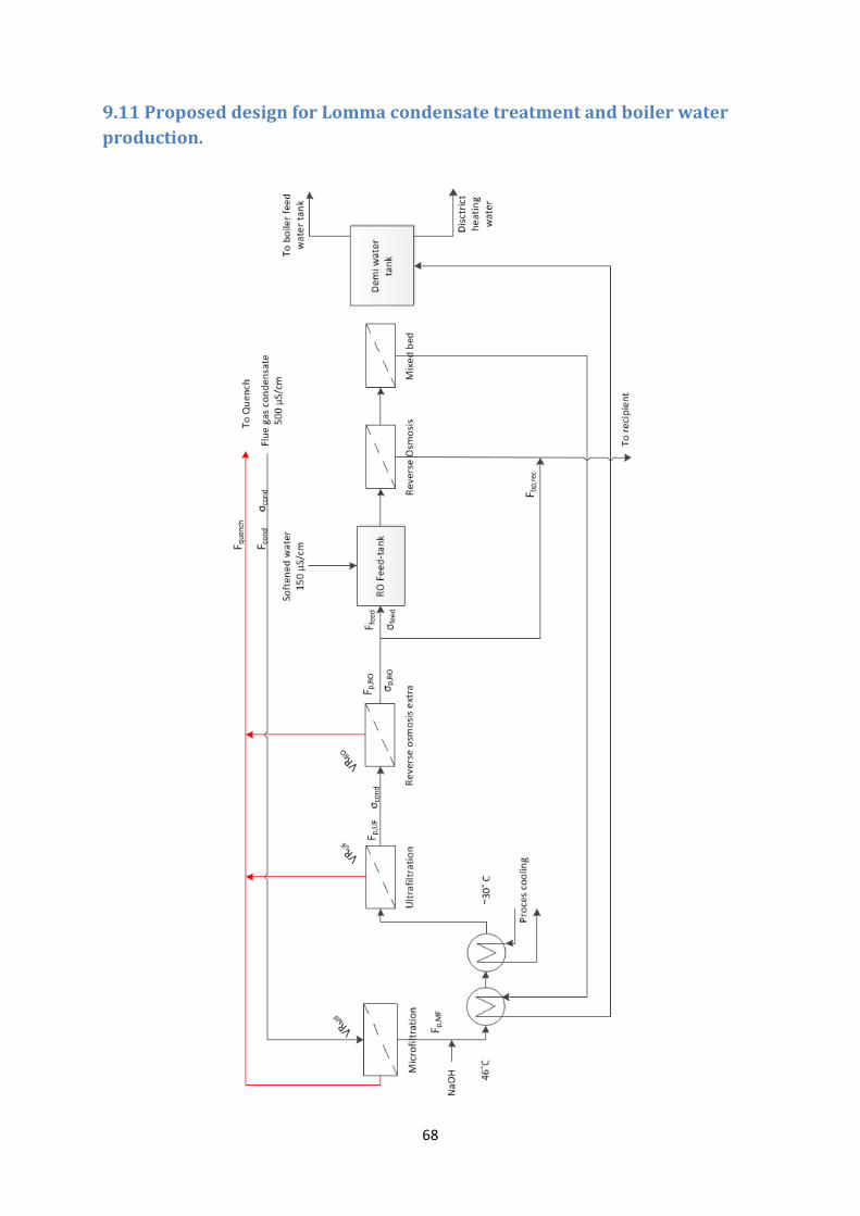
68

9.11 Proposed design for Lomma condensate treatment and boiler water

production.