designing distribution systems with reverse flows remanufactur (2017) 7:113–137 doi...
TRANSCRIPT

Jnl Remanufactur (2017) 7:113–137DOI 10.1007/s13243-017-0036-4
RESEARCH
Designing distribution systems with reverse flows
Ayse Cilacı Tombus1 · Necati Aras2 · Vedat Verter3
Received: 4 April 2017 / Accepted: 21 July 2017 / Published online: 4 October 2017© Springer Science+Business Media B.V. 2017
Abstract Closed-loop supply chains involve forward flows of products from productionfacilities to customer zones as well as reverse flows from customer zones back to remanufac-turing facilities. We present an integrated modeling framework for configuring a distributionsystem with reverse flows so as to minimize the total cost of satisfying customer demandand remanufacturing the returned items that are recoverable. Given a set of existing plantsand customer zones, our basic model identifies the optimal number and location of distri-bution centers and return centers assuming that all plants have remanufacturing capability.We devise a Lagrangian heuristic for this problem. The proposed solution method provedto be computationally efficient for solving large-scale instances of the closed-loop supplychain design problem. The potential benefits of the integrated model are demonstrated bycomparing its results with those obtained from an alternative approach that determines opti-mal forward and reverse network structures sequentially. We also extend the basic modelto determine the optimal locations for establishing remanufacturing facilities. Using theextended model, we study the conditions under which the return centers can be co-locatedwith remanufacturing facilities rather than being established at the downstream echelonsof the supply chain. Different from the existing works on facility location-allocation mod-els for closed-loop supply chain network design, the main focus in this paper is on theinvestigation of structural properties of the network such as co-locating return centers withremanufacturing facilities and quantifying the benefit of modeling forward and reverseflows simultaneously rather than sequentially.
� Necati [email protected]
1 Department of Industrial Engineering, Maltepe University, Istanbul, Turkey
2 Department of Industrial Engineering, Bogazici University, Istanbul, Turkey
3 Desautels Faculty of Management, McGill University, Montreal, Canada

114 Jnl Remanufactur (2017) 7:113–137
Keywords Reverse logistics · Facility location-allocation · Lagrangian relaxation ·Mixed-integer programming model
Introduction
The second half of the twentieth century witnessed the global rise of a consumption-basedeconomy. This trend resulted in an ever-increasing threat to environmental sustainabil-ity. Environmentally conscious manufacturing, waste reduction and product recovery haveemerged as alternative means of coping with this significant societal problem. In this paper,we focus on supply chains with product recovery, which aim at capturing the remainingeconomical value in used, unsold, or obsolete products. Based on a survey of nine casestudies on product recovery processes in different industries, Fleischmann et al. [11] high-light the following common activities: (i) collection of used products, (ii) inspection andseparation of the recoverable returns and those that need to be disposed due to economicand/or technological reasons, (iii) reprocessing the returns, which involves reuse, recycling,remanufacturing or repair, and (iv) redistribution of the recovered materials, components orproducts. From a logistics viewpoint, these activities create a reverse flow of goods fromconsumers toward upstream layers of the supply chain. The simultaneous presence of for-ward and reverse flows cause unique challenges for supply chain design, which we tackle inthis paper. To this end, we provide an analytical framework for making structural decisionspertaining to distribution systems with reverse flows.
Under pressure from environmental groups and society at large, governments areincreasingly involved in regulating product recovery, because it can serve as an effec-tive mechanism for sustaining the environment. The WEEE legislation in the EuropeanUnion [36] that became effective in February 2014, for example, requires manufactur-ers to establish environmentally sound recovery processes including remanufacturing forused electrical and electronic equipment. On the other hand, an increasing number of com-panies have been implementing comprehensive programs in order to reap the potentialbenefits of remanufacturing. According to the United States International Trade Commis-sion report prepared in October 2012 (USITC Publication 4356, [34]), United States wasthe world’s largest remanufacturer during the period of 2009-2011 with the total valueof remanufactured products exceeding $43 billion. Furthermore, the most remanufactur-ing intensive industries in the United States comprise aerospace, electrical and electronicequipment, locomotives, machinery, medical devices, motor vehicle parts, office furniture,and retreaded tires. Thanks to HP’s reuse and recycling programs, more than 80% of inkcartridges and 38% of LaserJet toner cartridges are produced with recycled plastic [14].Moreover, HP Planet Partners have recycled more than 3.3 billion pounds of productssince 1987. Xerox reports that their combined returns programs including equipment resaleand remanufacturing along with parts and consumable reuse and recycling prevented over38,000 metric tons of waste in 2003 which otherwise would end up in landfills [37].
Managing the flow of returned products from customer zones to remanufacturing facil-ities often involves the establishment and operation of return centers. A return centertypically offers scale economies in dealing with returned products in much the same waya distribution center plays a role in the distribution networks. It is well understood that thereturned products can have considerable variation in their quality level. This implies that theeconomic value that can be gained from these so-called cores can also vary. To cope withthese uncertainty, return centers perform a quality-based classification by means of inspec-tion and screening tests [4]. Those deemed recoverable are shipped to the remanufacturing

Jnl Remanufactur (2017) 7:113–137 115
facilities whereas the rest are either sent to recycling facilities or to landfill and incinerationsites for disposal.
A significant majority of the research on the design of reverse logistics (RL) networkshas focused on the structural decisions regarding the reverse distribution networks. Thelocation and sizing decisions associated with only the collection, inspection, recycling andremanufacturing facilities are incorporated in the proposed mathematical formulations. Arecent and comprehensive review on these papers, which do not incorporate the configu-rational decisions pertaining to the forward distribution network, can be found in [1, 13].There are 31 papers that are immediately relevant to our research since they incorporate theflows in both directions in making design decisions. We discuss this stream of research inmore detail in the next section.
This paper’s main contribution is a methodology for designing closed-loop supply chains(CLSCs) i.e., making structural decisions pertaining to both the forward and reverse dis-tribution networks simultaneously. To this end, we incorporate the presence of reverseflows, return centers and remanufacturing facilities in the well-known (single-commodity)production-distribution system design model. Using our modeling framework, we addresstwo important strategic questions. “Is there a significant benefit due to designing forwardand reverse networks simultaneously rather than sequentially?” and “Under which condi-tions can the return centers be co-located with remanufacturing facilities rather than beingestablished at the downstream echelons of the supply chain?” Through extensive computa-tional experiments, we find that the general level of capacity utilization in remanufacturingfacilities is a key factor determining the potential benefits of the integrated design approach.We also observe that the most appropriate echelon for return centers that perform inspectionand separation heavily depends on the overall quality and quantity of the returns collectedat the customer zones. On the algorithmic front, we study the effectiveness of Lagrangianrelaxation in solving the CLSC design models presented in the paper. Our computationalexperiments indicate that the Lagrangian relaxation is more efficient than CPLEX forlarge-scale problem instances.
The remainder of the paper is organized as follows. An overview of the most relevant lit-erature is provided in the next section. “The basic model” presents the integrated model fordesigning distribution systems with reverse flows and “Solution methodology” outlines theLagrangian heuristic for this problem. In “Computational experiments”, we implement theheuristic in solving a realistic case study and demonstrate its computational efficiency forlarge-scale problem instances. “Integrated versus sequential design” is devoted to the com-parison of alternative approaches to CLSC design in order to demonstrate the advantages ofthe proposed integrated approach. “Where to locate the return centers?” extends the basicmodel to determine whether the firm can benefit from establishing the return centers at theupstream echelon co-located with the remanufacturing facilities. We finish the paper withsome concluding remarks.
Detailed overview of the literature
The design of a CLSC is in fact related to the notion of supply chain integration (SCI). SCIrepresents the level at which a producer works together with its partners in the supply chainto generate an effective and efficient flow of products, information, services and value tothe customer. A possible categorization for integration is given in Pishvaee et al. [26] as“horizontal integration” and “vertical integration”. The former one refers to the integrationof problems at the same decision level such as strategic level or operational level, while the

116 Jnl Remanufactur (2017) 7:113–137
latter one involves considering the integration of problems at different decision levels. Forexample, tackling the supplier selection problem together with the network design problemis horizontal integration since both problems occur at the strategic level. Addressing networkdesign problem while taking into account vehicle routing issues for a distribution companycan be seen as vertical integration. In our setting, the design of CLSC where configurationaldecisions concerning both forward and reverse networks are involved is clearly horizontalintegration because the corresponding decisions are all pertinent to the strategic level.
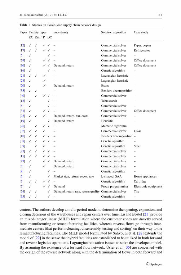
In this section, we focus on 31 papers that are immediately relevant to our work due totheir focus on the design of distribution systems with reverse flows by incorporating facil-ity location decisions. These papers are given in Table 1 and categorized with regard tothe network structure modeled, i.e., whether the designed network includes return centers(RC), remanufacturing facilities (RmF), manufacturing plants (P) and/or distribution centers(DC). We would like to emphasize that facility types called collection centers and inspec-tion centers in some studies are treated under the name “RC”. In Table 1, we also indicatewhat type of uncertainty is taken into account in the model, the solution approach/algorithmadopted, and whether the proposed methodology is implemented in a real-life case.
In an early effort, Marın and Pelegrin [22] extended the simple plant location problem todefine the return plant location problem where each manufacturing plant to be establishedalso serves as a collection center for customer returns. A more realistic extension of this verybasic network is considered in Beamon and Fernandes [5] where the manufacturing plantsserve the customer demand via warehouses and receive the returns via collection centersand warehouses. Fleischmann et al. [12] compare the sequential and integrated approachesfor the design decisions and by analyzing two hypothetical examples inspired by real-lifeindustrial cases the authors conclude that the reverse flows have a significant impact on theoverall network structure only when the forward and reverse channels differ in a consider-able way with respect to geographical distribution or cost structure. The authors also pointout that return volumes constitute a key factor in the design decisions.
Salema et al. [29] offer an alternative formulation where the flow variables are rep-resented at two levels (i.e., plant-warehouse and warehouse-customer) rather than thesingle level formulation of flow variables in Fleischmann et al. [12] (i.e., plant-warehouse-customer). In solving two cases, based on a document-office company in Spain and copierremanufacturing in Europe, the authors used the CPLEX solver within GAMS Suite. Anextended model is also provided for the capacitated and multi-product version of the designproblem, which was implemented for only two products during the case analysis. Salemaet al. [31] is an effort to incorporate tactical decisions, such as production and inventory lev-els, in the integrated RL network design. Extending their earlier formulation to represent aset of macro and micro time periods, Salema et al. [31] demonstrate that the arising modelcan handle fairly large problem instances encountered in practice. Later on, Salema et al.[32] build upon their previous work and propose a generalized model that yields a tacticalplan for acquisition, production, storage and distribution in a predefined time horizon inaddition to designing the supply chain considering simultaneously the forward and reverseflows.
In perhaps the most detailed case study for integrated RL network design, Krikkeet al. [17] focus on the forward and reverse supply chains of refrigerators and evaluate threealternative refrigerator designs from the perspective of their overall costs, energy consump-tion and waste generated. Ko and Evans [16] address the problem of a third-party logistics(3PL) provider which runs the warehouses and repair centers performing inspection andseparation activities. The client company operates a set of existing plants that aim at sat-isfying the market demand via the warehouses and collect the returns through the repair
Jnl Remanufactur (2017) 7:113–137 117
Table 1 Studies on closed-loop supply chain network design
Paper Facility types uncertainty Solution algorithm Case study
RC RmF P DC
[12] � � � � – Commercial solver Paper, copier
[17] � � � � – Commercial solver Refrigerator
[5] � � – Commercial solver –
[29] � � � – Commercial solver Office document
[30] � � � Demand, return Commercial solver Office document
[16] � � – Genetic algorithm –
[21] � � � – Lagrangian heuristic –
[28] � � – Lagrangian heuristic –
[20] � � Demand, return Exact –
[35] � � – Benders decomposition –
[40] � � � – Commercial solver –
[18] � � – Tabu search –
[8] � � – Commercial solver –
[31] � � � – Commercial solver Office document
[25] � � � Demand, return, var. costs Commercial solver –
[19] � � Demand, return Heuristic –
[26] � � � – Memetic algorithm –
[32] � � � – Commercial solver Glass
[10] � � � � – Benders decomposition –
[38] � � � � – Genetic agorithm –
[39] � � – Genetic algorithm Steel
[23] � � � � – Commercial solver –
[15] � � � � – Commercial solver –
[27] � � � Demand, return Commercial solver –
[3] � � Demand, return Commercial solver –
[9] � � – Genetic algorithm –
[6] � � Market size, return, recov. rate L-shaped, SAA Home appliances
[7] � � � � – Genetic algorithm Cartridge
[2] � � � Demand Fuzzy programming Electronic equipment
[24] � � � Demand, return rate, return quality Commercial solver Tire
[33] � � � – Genetic algorithm –
centers. The authors develop a multi-period model to determine the opening, expansion, andclosing decisions of the warehouses and repair centers over time. Lu and Bostel [21] providean mixed-integer linear (MILP) formulation where the customer zones are directly servedfrom manufacturing or remanufacturing facilities, whereas reverse flows go through inter-mediate centers (that perform cleaning, disassembly, testing and sorting) on their way to theremanufacturing facilities. The MILP model formulated by Sahyouni et al. [28] extends themodel of [22] in the sense that hybrid facilities are established to be utilized in both forwardand reverse logistics operations. Lagrangian relaxation is used to solve the developed model.By assuming the existence of a forward flow network, Uster et al. [35] are concerned withthe design of the reverse network along with the determination of flows in both forward and

118 Jnl Remanufactur (2017) 7:113–137
reverse channels. Their objective is to determine the locations of the collection centers andremanufacturing facilities along with the forward and reverse flows such that the sum of theprocessing, transportation, and facility location costs are minimized. Easwaran and Uster[10] incorporate capacitated Hybrid Centers (HCs) and Hybrid Sourcing Facilities (HSFs)into their existing models. HCs can play the role of both DCs and/or RCs and HSFs performboth manufacturing of new products and remanufacturing of used products. The aim of thedeveloped model is to determine the best locations of the HSFs and the HCs as well as thebest flow of products in the CLSC network.
Zhou and Wang [40] present a very similar model to that of Fleischmann et al. [12] inwhich returns can be repaired at centralized return centers and sent back to the warehousesto satisfy the customer demand. Lee and Dong [18] develop a Tabu search based heuris-tic for integrated RL network design in end-of-lease computers. In their model, there is asingle OEM who wants to establish a set of capacitated hybrid processing facilities thatserve as both DCs as well as collection centers. The same authors deal with a multi-periodlocation and allocation model where optimal locations for forward processing facilities, col-lection centers, and hybrid processing are sought under demand and return uncertainty [19].The solution approach adopted is based on sample average approximation method com-bined with a simulated annealing heuristic. Pishvaee et al. [25] investigate an integratedforward/reverse logistics network design problem in which the production/recovery centers,distribution/collection centers, and disposal centers are considered while taking into accountthe uncertainties about the demand, number of returns and variable costs. Pishvaee et al.[26] examine the effect of the capacity levels on logistics network efficiency and respon-siveness by formulating a multi-objective, multi-stage forward/reverse logistics networkdesign including production, distribution, collection/inspection, recovery and disposal facil-ities with multiple capacity levels. Wang and Hsu [38] propose a CLSC network includingrecovery and landfilling rates to integrate environmental issues into a traditional logisticssystem.
Zhang et al. [39] address a dynamic capacitated production planning problem in a steelcompany by means of a multi-echelon, multi-period and multi-product CLSC model. Ozkırand Baslıgil [23] incorporate material recovery, component recovery and product recoveryprocesses into design of a CLSC network to increase system profitability. Keyvanshokoohet al. [15] study a multi-echelon, multi-period, multi-commodity and capacitated integratedforward/reverse logistics network concerning the quality levels of the returned products andacquisition price offered according to return type. The paper by Rosa et al. [27] proposesa multi-period CLSC network model by allowing the locations of plants, DCs and RCsto be changed. The capacities of all the facilities can also be modified (i.e., increased ordecreased) during the planning horizon. The deterministic model is then extended to a robustoptimization model by taking into account the uncertainty in demand and return. Amin andZhang [3] first formulate a deterministic MILP model where plants and collection centersare opened and then extend it to a stochastic bi-objective model with demand and returnuncertainty. As the solution approach, they apply ε-constraint method and weighted sumsmethod.
Demirel et al. [9] examine a multi-period and multi-part MILP model for a capacitatedCLSC network under deterministic demand. They contribute to the literature by incor-porating second-hand sales, incremental incentives and inventory policies in the returnstreams of the CLCS network as well as the trade-offs between virgin parts and usedparts/products. Chen et al. [6] describe the existing cartridge recycling system in HongKong, which includes the classification of used products according to their quality level andthe delivery of different materials extracted from them. Chen et al. [7] deviate from other

Jnl Remanufactur (2017) 7:113–137 119
studies on CLSC network design and focus on the following two questions: How do theuncertainties in market size, return quantities and recovery rate affect the profitability ofthe CLSC and how is product recovery strategy influenced by the consumer perceptionof remanufactured products and variable cost structure. To this end, the authors develop astochastic mixed-integer quadratic model use a solution approach based on an integrationof the integer L-shaped decomposition with sample average approximation which enablesto handle many scenarios.
Shi et al. [33] develop a multi-objective an MILP model for a CLSC network designproblem. In addition to the overall costs, the model optimizes overall carbon emissions andthe responsiveness of the network. An improved genetic algorithm based on the frameworkof nondominated sorting genetic algorithm (NSGA II) is developed to obtain Pareto-optimalsolutions. In their paper, Pedram et al. [24] examine a CLSC model for tire industry withdemand and return uncertainty where both forward and reverse chain consists of three lay-ers. In particular, collection centers, retreading centers and recycling centers constitute thefacilities in the reverse channel. Amin and Baki [2] propose a bi-objective CLSC modelin which one objective is on-time delivery maximization from the suppliers and the otherobjective is profit maximization. There exists uncertainty in the demand and factors such asexchange rates and customs duties are also taken into account which differentiates this studyfrom other works. Moreover, a case study is presented involving electrical and electronicequipments.
As can be seen, the first research question we pose is partially examined by Fleischmannet al. [12] where two different real CLSCs are compared and it is shown that integrateddesign may be beneficial depending on the difference between forward and reverse chan-nels. However, there is no systematic analysis regarding the amount of the resulting benefitbased on the relevant parameters. Our paper is an attempt towards filling this gap. The sec-ond research question we investigate is somehow covered in Easwaran and Uster [10]. But,in that paper DCs are necessarily co-located with RCs, which means that once an RC is co-located with a remanufacturing facility, there is also a DC established there. We believe thatthis is rather a restrictive assumption. Therefore, in our paper, we look at the co-locationissue only in terms of the facilities handling reverse flows, i.e., remanufacturing facilitiesand RCs.
The basic model
In this section, we present a basic model that incorporates reverse flows as well as the asso-ciated RCs in the distribution network design problem. Based on a set of existing plants(each with given manufacturing and remanufacturing capacities) and a set of customer zones(each with given demand and return quantities for a single product), the model determinesthe optimal number and location of the DCs and RCs so as to minimize the total cost ofestablishing and operating this closed-loop network. The model requires that all the demandis met and all the returns are collected at the customer zones. Therefore, the total numberof manufactured and remanufactured products must be sufficient to satisfy the demand atthe customer zones and the total remanufacturing capacity must be large enough to processall the remanufacturable returns. We assume no capacity limit for the DCs and RCs to beestablished. In developing the model, our focus has been to understand the nature of theflows and the associated DC/RC configuration in the closed-loop network. To refrain fromintroducing any plant-based bias into the solution, we assume that both the unit manufac-turing cost and the unit remanufacturing cost (which is lower) are the same at all facilities.

120 Jnl Remanufactur (2017) 7:113–137
These costs can be omitted from the model since the total quantities to be manufactured andremanufactured are pre-determined. The basic model is extended in the sequel to alsoincorporate the location decisions pertaining to the establishment of remanufacturingfacilities.
Using the index set i for plants, j for DCs as well as RCs and k for customer zones, wedefine the following decision variables:
Yj ={
1 if a DC is located at site j
0 otherwise
Tj ={
1 if an RC is located at site j
0 otherwise
Xjk = annual amount shipped from DC j to customer zone k
Wkj = annual amount shipped from customer zone k to RC j
Uij = annual amount shipped from plant i to DC j
Vji = annual amount shipped from RC j to plant i
The following is the list of model parameters, which are also depicted in Fig. 1.
fj = (annualized) fixed cost of opening a DC at site j
gj = (annualized) fixed cost of opening an RC at site j
cij = cost of shipping one unit from plant i to DC j
ejk = cost of shipping one unit from DC j to customer zone k
c′ji = cost of shipping one unit from RC j to plant i
e′kj = cost of shipping one unit from customer zone k to RC j
dk = annual demand at customer zone k
rk = annual return at customer zone k
α = recovery ratio (fraction of returns found to be remanufacturable after inspection)si = manufacturing capacity of plant i
ai = remanufacturing capacity of plant i
The problem can now be formulated as an MILP.
Fig. 1 The closed-loop network model and its parameters

Jnl Remanufactur (2017) 7:113–137 121
Problem P
ZP = min∑j
fjYj +∑j
gjTj +∑i
∑j
cijUij +∑j
∑k
ejkXjk+∑j
∑i
c′jiVji +∑
k
∑j
e′kjWkj
s.t.
∑j
Xjk = dk ∀k (1)
∑j
Wkj = rk ∀k (2)
∑k
Xjk =∑
i
Uij ∀j (3)
α∑
k
Wkj =∑
i
Vji ∀j (4)
∑j
Uij −∑j
Vji ≤ si ∀i (5)
∑j
Vji ≤∑j
Uij ∀i (6)
∑j
Vji ≤ ai ∀i (7)
Xjk ≤ dkYj ∀j, k (8)
Wkj ≤ rkTj ∀j, k (9)
Xjk, Wkj , Uij , Vji ≥ 0 ∀i, j, k (10)
Yj , Tj ∈ {0, 1} ∀j (11)
The objective function includes the transportation cost of both forward and reverse flowsand the fixed cost of opening DCs and RCs. Constraints (1) ensure that the demand ofeach customer is satisfied, whereas constraints (2) impose that all the returns are collected.Due to the existing manufacturing and remanufacturing capacities, single-sourcing of eachcustomer by a DC and/or an RC cannot be expected. Constraints (3) and (4) are the flowconservation equations at DCs and RCs, respectively. Note that the amount of returns to beshipped from an RC to the plants is only a fraction of the returns arriving at the RC, denotedby α, and the remainder of the returns are to be disposed of. Since this recovery ratio isa proxy for the overall quality of returns, α does not vary with the RC location. Thus, thetotal amount of disposals is pre-determined and by assuming that the unit disposal costs arethe same at all RCs we leave disposal costs out of the model. Constraints (5) ensure thatthe number of manufactured products is bounded by the manufacturing capacity, whereasconstraints (7) guarantee that remanufacturing capacity is not exceeded at each plant. Inorder to sustain the closed-loop nature of the network, each plant needs to remanufactureall the incoming returns and ship them off to the DCs as part of the forward flows. Sinceremanufacturing is cheaper than manufacturing on the average, each plant will naturallyprioritize processing the returns from RCs. Nonetheless, lower transportation costs betweenother plant-DC pairs may impede a plant’s ability to ship all the remanufactured goods.To prevent such build-up of remanufactured goods inventories at the plants, we imposeconstraints (6). Constraints (8) and (9) guarantee that customers can only be assigned to
122 Jnl Remanufactur (2017) 7:113–137
open DCs and open RCs, respectively. Constraints (10) and (11) are the nonnegativity andintegrality constraints, respectively.
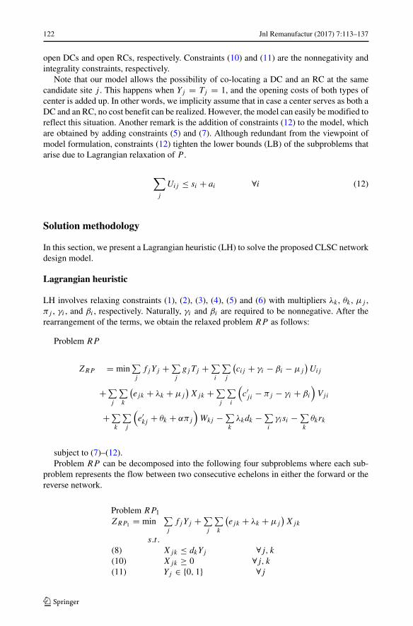
Note that our model allows the possibility of co-locating a DC and an RC at the samecandidate site j . This happens when Yj = Tj = 1, and the opening costs of both types ofcenter is added up. In other words, we implicity assume that in case a center serves as both aDC and an RC, no cost benefit can be realized. However, the model can easily be modified toreflect this situation. Another remark is the addition of constraints (12) to the model, whichare obtained by adding constraints (5) and (7). Although redundant from the viewpoint ofmodel formulation, constraints (12) tighten the lower bounds (LB) of the subproblems thatarise due to Lagrangian relaxation of P .
∑j
Uij ≤ si + ai ∀i (12)
Solution methodology
In this section, we present a Lagrangian heuristic (LH) to solve the proposed CLSC networkdesign model.
Lagrangian heuristic
LH involves relaxing constraints (1), (2), (3), (4), (5) and (6) with multipliers λk , θk , μj ,πj , γi , and βi , respectively. Naturally, γi and βi are required to be nonnegative. After therearrangement of the terms, we obtain the relaxed problem RP as follows:
Problem RP
ZRP = min∑j
fjYj +∑j
gjTj +∑i
∑j
(cij + γi − βi − μj
)Uij
+∑j
∑k
(ejk + λk + μj
)Xjk +∑
j
∑i
(c′ji − πj − γi + βi
)Vji
+∑k
∑j
(e′kj + θk + απj
)Wkj −∑
k
λkdk −∑i
γisi −∑k
θkrk
subject to (7)–(12).Problem RP can be decomposed into the following four subproblems where each sub-
problem represents the flow between two consecutive echelons in either the forward or thereverse network.
Problem RP1
ZRP1 = min∑j
fjYj +∑j
∑k
(ejk + λk + μj
)Xjk
s.t.
(8) Xjk ≤ dkYj ∀j, k
(10) Xjk ≥ 0 ∀j, k
(11) Yj ∈ {0, 1} ∀j

Jnl Remanufactur (2017) 7:113–137 123
Problem RP2
ZRP2 = min∑i
∑j
(cij + γi − βi − μj
)Uij
s.t.
(10) Uij ≥ 0 ∀i, j
(12)∑j
Uij ≤ si + ai ∀i
It is important that constraints (12) ensure finite values for variables Uij in subproblem RP2.In the absence of (12), the Uij values and hence RP2 will be unbounded.
Problem RP3
ZRP3 = min∑j
gjTj +∑k
∑j
(e′kj + θk + απj
)Wkj
s.t.
(9) Wkj ≤ rkTj ∀j, k
(10) Wkj ≥ 0 ∀j, k
(11) Tj ∈ {0, 1} ∀j
Problem RP4
ZRP4 = min∑j
∑i
(c′ji − πj − γi + βi
)Vji
s.t.
(7)∑j
Vji ≤ ai ∀i
(10) Vji ≥ 0 ∀i, j
All the four subproblems can be solved by inspection as shown in Appendix 1, and theobjective value of the relaxed problem provides a lower bound on the optimal objectivevalue ZP of the original problem P for any multiplier vectors λ, θ , μ, π , γ , and β. To findthe best lower bound, we have to solve the Lagrangian dual:
maxλk,θk,μj ,πj ,γi≥0,βi≥0
ZRP = ZRP1 +ZRP2 +ZRP3 +ZRP4 −∑
k
λkdk −∑
i
γisi −∑
k
θkrk
We use subgradient optimization in updating the multipliers at each iteration of the algo-rithm, which terminates after t ′0 iterations or a pre-specified CPU time. A formal statementof the Lagrangian heuristic is provided in Appendix 2. The solutions to RP1 and RP3 pre-scribe a set of open DCs and a set of open RCs. By fixing the binary variables to representthese open DCs and RCs, a feasible solution for problem P can be found by solving a simpletransshipment problem. If the binary location variables for distribution centers and returncenters (i.e., variables Yj and Tj ) are set to known values as a result of solving subprob-lems RP1 and RP3, then the MILP problem P reduces to linear programming problem withcontinuous decision variables representing the amount of flow between plants and DCs aswell as DCs and customer zones in the forward network, and between customer zones andRCs as well as RCs and plants in the reverse network. Since it is a linear program, it canbe easily solved using commercial solver CPLEX. The objective value of this solution ZUB
P
provides an upper bound (UB) on the optimal objective value of P.
Computational experiments
In this section, we first apply LH to solve a realistic case study and then assess itsperformance in solving a set of larger-scale problem instances.

124 Jnl Remanufactur (2017) 7:113–137
A realistic case study
We study the performance of LH in solving a realistic case study that is based on the copierremanufacturing case in Fleischmann et al. [12]. The original case models 50 Europeancities with a population of over 500,000 as customer zones. In an effort to use up-to-datepopulation data, we searched wikipedia.org and nationsonline.org and identi-fied 63 European cities with more than 500,000 inhabitants, 27 of which are the nationalcapitals. We assume that there is a plant at each of the 27 capitals, and the 63 major citiesconstitute the set of alternative sites for the DCs and RCs to be established. Consequently,our case is an I27,63,63 instance of the network design problem.
The model parameters were set to the values in Fleischmann et al. [12]. The fixed costs ofestablishing DCs and RCs are fj =1,500,000 and gj = 500,000 Euros. The unit transportcosts per kilometer are cij = 0.0045, ejk = 0.01, c′
ji = 0.005 and e′kj = 0.003 Euro. The
demand per 1,000 inhabitants is 10 units (i.e., dk = population /100), whereas the return andrecovery ratios are τ = 0.6 and α = 0.5, respectively. Since there is no capacity informationin the original case, we experimented with three capacity levels for the manufacturing andremanufacturing facilities at each plant. Let n denote the number of plants. We compute thethree alternative capacity levels using the formulae below:
ai =⌊
a′ατ∑
kdk
n
⌋and si =
⌊(s′∑
kdk − nai
)n
⌋(13)
where the capacity parameters (a′, s′) take the values (1.5, 1.2), (3.0, 2.4), and (4.5, 3.6)
for low, medium, and high capacity levels, respectively.Table 2 compares the performance of LH with that of CPLEX. The percent deviation
from the optimal objective value z is denoted by “%” and it is calculated as 100 × (UB −z)/z. We observe that the problem instance becomes more difficult to solve as the manu-facturing and remanufacturing capacities are reduced. For the most challenging instance,which has the lowest capacity levels, LH provides a solution that is within 6.1 percent ofthe optimal solution obtained by CPLEX, albeit it requires about twice the computationtime. Perhaps more importantly, CPLEX requires almost triple the time to solve the lowcapacity instance compared to that of the high capacity instance, whereas the computationalrequirement increases only 27% for the proposed algorithm.
By studying the optimal sets of DC and RC locations, we conclude that the model is notrobust with respect to the manufacturing and remanufacturing capacity levels. It is optimal
Table 2 Results for the case study
Capacity CPLEX Lagrangian relaxation
Level z CPU LB UB % CPU
Low 14,993.4 40.97 13,442.5 15,912.5 6.13 77.75
Medium 14,118.0 22.72 12,850.6 14,641.9 3.71 73.75
High 13,716.6 14.84 12,692.6 13,998.1 2.05 61.11
Jnl Remanufactur (2017) 7:113–137 125
to establish three DCs and co-locate the RCs with these facilities for all capacity levels.Two out of three sites are common for the low and medium capacities, whereas a set ofcompletely different cities is used for the high capacity levels. We also find that the modelis not robust with respect to the solution quality. While LH provides solutions between2% and 6.1% of the optimal objective value as the capacity levels are varied, none of thesites in the heuristic solution are the same as those in the optimal solution of the sameinstance. We also solved the case with lower return and recovery ratios i.e., τ = 0.3 andα = 0.2, respectively. The optimal solution in this case is to open a single RC at the samelocation regardless of the capacity levels (of course, the optimal DC sites do not change).Interestingly, this dominant single RC site is not included in any of the three solutions forthe original τ = 0.6 and α = 0.5 instance. This implies that a greedy heuristic may notwork well for this closed-loop supply chain design problem.
This I27,63,63 problem can be considered as a medium-scale instance, and we demonstratethe performance of the proposed Lagrangian relaxation procedure in solving large-scaleinstances in the next section.
Solving large-scale problem instances
We generate 24 problem instances by fixing the number of plants at 20 and setting the num-ber of customer zones to 100, 200, 400, and 800. Since each customer zone is consideredas an alternative DC/RC site, we in fact can group these 24 instances in four sets which wecall I20,100,100, I20,200,200, and I20,400,400 in the sequel. The (x, y) coordinates for the plants,potential DC/RC sites and customer zones in each set are generated through uniformly dis-tributed random numbers in [0, 1]. The unit transportation costs are estimated using theEuclidean distance between the facility pairs in consecutive echelons. Therefore, the unitcosts of forward and reverse flows are equal for a given pair of sites. For example, the unitcost of shipping goods from plant 1 to a DC at site 2 (c12) is the same as the unit cost oftransporting returned products from an RC at site 2 to plant 1 (c′
21). The demand at eachcustomer zone is generated from a uniform distribution between 50 and 100 units. For theease of exposition we assume that the return ratio τ = rk/dk is the same for all k. For eachset, we compute three manufacturing and remanufacturing capacity levels using (13) anduse two levels for the fixed costs of establishing DCs and RCs. These are set at $50 and $75,respectively as the low level and $500 and $750, respectively as the high level. The returnratio and the recovery ratio are taken as τ = 0.5 and α = 0.5, respectively. The Lagrangianheuristic has been coded in Matlab 7.4.0 R2007a and the computational experiments wererun on a computer with Intel Xeon CPU X5460 at 3.16 GHz processor and 16 GB of RAM.We set a 7,200 seconds time limit for CPLEX.
Table 3 reports on our computational results of the closed-loop supply chain design prob-lem. Four instances could not be solved to optimality within the allowed CPU time. Forthese more challenging instances, the best solutions identified by CPLEX are reported inthe table (each indicated by “∗”).
Table 3 confirms our earlier observation that problem complexity increases as the capac-ity levels are reduced. In addition, we found out that problem instances with higher fixedcosts are more difficult than their counterparts with lower fixed costs. Accordingly, CPLEXcould not solve two of the three most challenging “high fixed cost-low capacity” instancesto optimality within the allowed CPU time. In addition, the other two “high fixed cost”instances of the I20,400,400 problem could not be solved to optimality by CPLEX. Note that

126 Jnl Remanufactur (2017) 7:113–137
Table 3 Performance of LH for large-sized problems
Problem Fixed Capacity CPLEX LH
Cost Level z CPU LB UB % CPU
20-100-100 Low Low 2772.6 86.84 2521.6 2949.5 6.38 100.89
Low Medium 2483.5 4.42 2443.6 2487.7 0.17 122.44
Low High 2436.8 1.89 2392.0 2436.8 0.00 137.09
High Low 6262.7 726.30 5237.6 6536.5 4.36 88.06
High Medium 5637.7 181.81 5002.9 5783.5 2.59 87.77
High High 5401.8 80.86 4951.4 5490.2 1.64 83.53
20-200-200 Low Low 4019.8 758.27 3616.0 4155.0 3.36 783.50
Low Medium 3744.8 21.20 3706.1 3766.5 0.58 743.86
Low High 3723.1 11.16 3661.1 3756.8 0.90 525.89
High Low 9297.0 7200* 7507.9 9647.4 3.77 413.53
High Medium 8340.4 5365.36 7315.4 8545.6 2.46 390.08
High High 7985.9 3767.36 7181.6 8092.6 1.34 386.17
20-400-400 Low Low 5802.8 3011.91 4848.0 5982.6 3.10 8055.53
Low Medium 5308.1 89.94 5079.4 5606.3 5.62 4848.52
Low High 5278.1 10.28 4981.8 5809.9 10.08 3165.80
High Low 20,058.8 7200* 9945.0 14,017.1 −30.12 3669.97
High Medium 17,013.6 7200* 9988.4 12,099.9 −28.88 2491.27
High High 11,914.7 7200* 9887.1 11,679.9 −1.97 2761.83
LH performs better than CPLEX for the three “high fixed cost” instances of the largestscale problems we have solved (indicated by the negative % values in Table 3). Notably,the solutions provided by the proposed Lagrangian heuristic for two I20,400,400 instances are29–30% better than the best solution identified by CPLEX and these heuristic solutions areobtained by spending much less computational time.
Integrated versus sequential design
In the previous sections we studied an integrated design approach, which involves simul-taneous decisions regarding the location of DCs and RCs as well as forward and reverseflows in the closed-loop supply chain. An alternative to our approach is sequential design,which involves first making the DC location and forward flow decisions without incorporat-ing the reverse flows, and then configuring the reverse supply chain by taking the forwardchain structure as given [12]. This is particularly relevant for the firms with an existing for-ward supply chain and considering the launch of product recovery initiatives. In this section,we compare these two approaches in an effort to highlight the potential benefits of inte-grated design. We address the following question: “Is there a significant difference betweenintegrated and sequential design in terms of cost and solution structure?”
The sequential design approach is represented by the forward problem PF and the reverseproblem PR defined below. Note that constraints (5) are revised as (5′) in PF since there are

Jnl Remanufactur (2017) 7:113–137 127
no reverse flows in this formulation, i.e., Vji = 0. Also, the optimal forward flows U∗ij are
used in constraints (6′) of PR to limit the reverse flows into a plant.
PF : min∑j
fjYj +∑i
∑j
cijUij +∑j
∑k
ejkXjk
s.t (1), (3), (8)∑j
Uij ≤ si ∀i (5′)
Xjk, Uij ≥ 0 ∀i, j, k (10)
Yj ∈ {0, 1} ∀j (11)
PR : min∑j
gjTj +∑j
∑i
c′jiVji +∑
k
∑j
e′kjWkj
s.t (2), (4), (7), (9)∑j
Vji ≤ ∑j
U∗ij ∀i (6′)
Wkj , Vji ≥ 0 ∀i, j, k (10)
Tj ∈ {0, 1} ∀j (11)
In comparing the integrated and sequential design approaches, we first study the impact ofthe quantity and quality of the returns. Note that the return ratio τ at the customer zonesis a measure of return quantity, whereas the recovery ratio α at the RCs is a proxy forreturn quality. For the ease of studying the solutions in detail and tracking the changesduring the parametric analysis, we use a randomly generated I5,10,20 instance with fixedcosts (fj , gj ) = (50, 50). The total demand
∑kdk = 1455 for this instance, and hence
the total amount of reverse flows into the plants is 1455ατ . Although the other 15 I5,10,20instances we have solved are not discussed here in the interest of space, we remark that theobserved patterns are similar.
We set recovery ratio α = 0.6, manufacturing capacity si = 300, and remanufacturingcapacity ai = 200 for all plants, while varying the return ratio τ in the range (0, 1] withincrements of 0.1. Table 4 depicts the (optimal) total costs for integrated and sequentialdesign as well as the associated forward and reverse cost components. The last column indicatesthe percent cost savings that can be achieved by integrated design under each scenario.
Table 4 Impact of varying return ratio τ for α = 0.6
τ Integrated design cost Sequential design cost Percent
Forward Reverse Total Forward Reverse Total Saving
0.1 828.2 111.8 940.0 855.5 111.8 967.4 2.8
0.2 800.1 173.6 973.7 855.5 173.6 1029.2 5.4
0.3 764.1 246.8 1010.9 855.5 246.8 1102.3 8.3
0.4 748.0 303.2 1051.2 855.5 303.2 1158.8 9.3
0.5 737.7 360.7 1098.3 855.5 360.7 1216.2 9.7
0.6 737.7 427.0 1164.7 855.5 427.0 1282.6 9.2
0.7 737.7 487.8 1225.5 855.5 487.8 1343.4 8.8
0.8 738.0 541.4 1279.3 855.5 541.4 1396.9 8.4
0.9 738.6 601.2 1339.8 855.5 601.2 1456.7 8.0
1 763.8 685.1 1448.9 855.5 685.1 1540.6 6.0

128 Jnl Remanufactur (2017) 7:113–137
Table 5 Open DCs and RCs in integrated and sequential designs
τ 0.1 0.2 0.3 0.4 0.5 0.6 0.7 0.8 0.9 1.0
Integ. For. 6,7,9,10 6,7,9 3,6,7 1,3,6 1,3,6 1,3,6 1,3,6 1,3,6 1,3,6 1,3,6
Design Rev. 6 6 6 3,6 3,6 3,6 3,6,7 3,6,7 3,6,7 3,6,7
Seq. For. 7,9,10 7,9,10 7,9,10 7,9,10 7,9,10 7,9,10 7,9,10 7,9,10 7,9,10 7,9,10
Design Rev. 6 6 6 3,6 3,6 3,6 3,6,7 3,6,7 3,6,7 3,6,7
In the sequential approach, the optimal objective value of the forward problem does notvary with the return ratio τ because reverse flows are not incorporated in PF . The reverselogistics costs, however, increase with τ in both approaches since more returns need to beshipped back from customer zones. More importantly, the optimal reverse costs in the twoapproaches are the same in Table 4, whereas the optimal forward cost of the integrateddesign is always lower than that of the sequential design. That is, the cost disadvantage ofthe sequential design approach is due to the forward network (i.e., DC locations and forwardflows) rather than the reverse network (i.e., RC locations and reverse flows). The open DCsand RCs in both designs are depicted in Table 5. Note that the integrated design has theability to adapt the forward network configuration according to the return ratio.
We now focus on the costs related to forward flows. In Table 4, the optimal forward costfirst decreases and then increases with respect to the return ratio τ . This can be explainedin terms of the overall level of remanufacturing capacity utilization. Clearly, remanufac-turing capacity is under-utilized for low values of τ . For example, when τ = 0.2 only174 units need to be remanufactured which amounts to 17.5 percent utilization of the over-all remanufacturing capacity (given that α = 0.6, ai = 200 and there are five plantsin this instance). Therefore, as τ increases, the additional returns can be sent to thoseremanufacturing facilities that are in the plants with smaller forward costs. Thus, the reman-ufacturing capacity at such plants provides additional capability to serve the customerdemand through cheaper forward channels (e.g., plant-DC combinations) and to reduce theforward costs. When these remanufacturing facilities are fully utilized, however, furtherincreases of τ make the use of expensive forward channels inevitable (in Table 4 whenτ > 0.7). The forward cost curve behaves similarly for other values of α as shown inFig. 2. For α = 0.2 and 0.4 the forward cost curves are nonincreasing since the remanu-facturing capacity remains significantly under-utilized as the return ratio increases. Also,for α = 0.8 there is no feasible solution to the integrated problem when τ > 0.9. Thisis because the total remanufacturing capacity is insufficient to process all the recoverablereturns (i.e., 1455 × 0.8 × 0.9 = 1048 > 1000 = 5 × 200). In Fig. 3, the forward cost isdepicted as a function of the recovery ratio α for fixed values of the return ratio τ. Note thatthe forward cost curves in Figs. 2 and 3 demonstrate the same patterns. This is expectedsince it is the product of the return ratio and the recovery ratio that determines the number ofitems to be remanufactured and consequently the overall utilization of the remanufacturingcapacity.
Based on the above observations, we shift our focus on the effect of manufacturing capac-ity si and remanufacturing capacity ai on the percent cost difference between the integratedand sequential design approaches. For this set of experiments, we fix τ = 0.5 and α = 0.6in which case 30 percent of all the demand can be satisfied by remanufacturing returnedproducts. Note that integrated design outperforms sequential design by 9.7 percent for thisparameter setting when si = 300 and ai = 200 (see Table 4).

Jnl Remanufactur (2017) 7:113–137 129
Fig. 2 Forward cost of the integrated design for varying return ratios
We vary the remanufacturing capacity ai while manufacturing capacity is fixed atsi = 300. The optimal costs provided by the two design approaches as well as the percentcost differences are depicted in Table 6. At ai = 90, the total remanufacturing capacity of450 is still sufficient to process all the 437 recoverable returns (i.e., 1455×0.5×0.6). Con-sistent with our earlier observations, the increase in remanufacturing capacity has no impacton the total forward cost in sequential design and the total reverse costs are the same forboth approaches. The reverse costs decrease as remanufacturing capacity increases sincethe cheaper reverse channels (e.g., RC-plant combinations) can be used for a larger portionof the recoverable returns. More importantly, Table 6 confirms our earlier findings regard-ing the impact of remanufacturing capacity utilization on the forward costs of integrateddesign. Increasing ai reduces the overall utilization level, which enables increased use ofthe remanufacturing facilities at plants with smaller forward costs.
Our computational experiments on the same problem instance to study the impact ofvarying the manufacturing capacity si are summarized in Table 7. We observe that fora given value of the remanufacturing capacity ai the cost savings obtained by integrateddesign decrease as the manufacturing capacity increases. Although increasing manufac-turing capacity enables the use of cheaper plant-DC combinations in both integrated andsequential design, the forward costs decrease faster in the latter case. This can be attributedto the fact that integrated design is constrained to take into account the reverse flows in
Fig. 3 Forward cost of the integrated design for varying recovery ratios

130 Jnl Remanufactur (2017) 7:113–137
Table 6 Impact of varying remanufacturing capacity ai for si = 300
Integrated design cost Sequential design cost Percent
ai Forward Reverse Total Forward Reverse Total Saving
90 793.7 434.9 1228.6 855.5 434.9 1290.4 4.8
100 778.9 417.2 1196.1 855.5 417.2 1272.7 6.0
150 752.2 378.5 1130.7 855.5 378.5 1234.0 8.4
200 737.7 360.7 1098.3 855.5 360.7 1216.2 9.7
250 731.0 354.0 1085.0 855.5 354.0 1209.6 10.3
300 731.0 354.0 1085.0 855.5 354.0 1209.6 10.3
deciding the forward network structure. Again, the reverse costs are the same for both designapproaches.
During the computational experiments, we observed that optimal configuration and costof the reverse network seem to be robust with respect to the design approach. Note that thesame sets of RCs are opened by both integrated and sequential approaches under all τ , α andcapacity values in Tables 4–7. Parametric analysis on the other I5,10,20 instances we studiedby varying τ values confirm this observation.
Where to locate the return centers?
The preceding discussion assumes that the firm has a policy of locating RCs in the sec-ond echelon. An alternative strategy would be to co-locate the RCs with remanufacturingfacilities in the first echelon. This option has the fixed cost advantage due to the possiblescale economies associated with co-location. These savings, however, may be offset by the
Table 7 Impact of varying manufacturing capacity si
Integrated design Sequential design
Forw. Rev. Total Open Forw. Rev. Total Open Percent
ai si Cost Cost Cost DCs Cost Cost Cost DCs Diff.
100 300 778.9 417.2 1196.1 3,6,7 855.5 417.2 1272.7 7,9,10 6.0
325 771.4 417.2 1188.6 1,3,6,9 832.7 417.2 1249.9 6,7,9,10 4.9
350 766.0 417.2 1183.2 1,3,6,9 800.8 417.2 1218.0 6,7,9 2.9
375 757.6 417.2 1174.8 1,3,6 774.9 417.2 1192.1 3,6,7 1.5
150 300 752.2 378.5 1130.7 1,3,6,9 855.5 378.5 1234.0 7,9,10 8.4
325 746.6 378.5 1125.0 1,3,6 832.7 378.5 1211.2 6,7,9,10 7.1
350 737.7 378.5 1116.1 1,3,6 800.8 378.5 1179.3 6,7,9 5.4
375 728.8 378.5 1107.3 1,3,6 774.9 378.5 1153.4 3,6,7 4.0
200 300 737.7 360.7 1098.3 1,3,6 855.5 360.7 1216.2 7,9,10 9.7
325 728.8 360.7 1089.5 1,3,6 832.7 360.7 1193.3 6,7,9,10 8.7
350 720.1 360.7 1080.8 1,3,6 800.8 360.7 1161.5 6,7,9 6.9
375 711.4 360.7 1072.0 1,3,6 774.9 360.7 1135.6 3,6,7 5.6
Jnl Remanufactur (2017) 7:113–137 131
increased transportation costs since the unrecoverable returns are no longer disposed of atthe second echelon. In this section, we address the question “Under which conditions wouldthe integration of inspection and remanufacturing operations be beneficial?”
In order to compare the two policies mentioned above, we extend our original model(which assumes remanufacturing capability at all plants) so as to identify the optimal loca-tions for remanufacturing. This can easily be incorporated in Problem P by defining a newbinary variable Hi which takes the value one if a remanufacturing facility is located at planti and zero otherwise. We also let hi denote the fixed cost of opening a remanufacturing facil-ity at plant i. The resulting downstream problem PD represents the policy of locating RCs inthe second echelon. To capture the decisions pertaining to the establishment of remanufac-turing capacity at the existing plants, constraints (7) need to be modified as (7′) . ProblemPD can be solved via the Lagrangian heuristic presented in “Solution methodology”.
PD : min∑j
fjYj +∑j
gjTj +∑i
hiHi +∑i
∑j
cijUij +∑j
∑k
ejkXjk+∑j
∑i
c′jiVji +∑
k
∑j
e′kjWkj
s.t. (1)–(6), (8)–(10)∑j
Vji ≤ aiHi ∀i (7′)
Yj , Tj , Hi ∈ {0, 1} ∀i, j (11′)
In formulating the upstream problem PU we assume that the returns are sent from cus-tomer zones to the RCs at the remanufacturing facilities through the DCs. This is a plausibleassumption in many cases since the firms often use the same vehicles to deliver customerorders and collect returns. As a result, the DCs serve as consolidation centers for returnsfrom different customer zones. We define a new variable Li = 1 if an RC and a remanufac-turing facility is co-located at plant i and zero otherwise. The fixed cost of this integratedfacility is represented by li . The following formulation of the upstream problem PU alsoreflects that the unrecoverable returns are disposed of at the first echelon.
PU : min∑j
fjYj +∑i
liLi +∑i
∑j
cijUij +∑j
∑k
ejkXjk +∑j
∑i
c′jiVji +∑
k
∑j
e′kjWkj
s.t (1), (2), (3), (8), (10)∑k
Wkj = ∑i
Vji ∀j (4′)∑j
Uij − α∑j
Vji ≤ si ∀i (5′′)
α∑j
Vji ≤ ∑j
Uij ∀i (6′′)
α∑j
Vji ≤ aiLi ∀i (7′′)
Wkj ≤ rkYj ∀j, k (9′)Yj , Li ∈ {0, 1} ∀i, j (11′′)
In the computational experiments we use the same I5,10,20 instance with the followingparameter values: si = 300, ai = 200,
(fj , gj , hi
) = (50, 75, 100). We calculate the opti-mal cost of the upstream and downstream models for return ratio τ and recovery ratio α inthe range (0, 1] with increments of 0.2 and li ∈ {125, 150, 175}. Table 8 shows the resultsin terms of the percent cost difference with respect to the downstream model. That is, thenegative and bold numbers indicate that the optimal cost of the upstream model is less thanthat of the downstream model. The instances indicated with “–” are infeasible because thetotal number of recoverable returns is greater than the total remanufacturing capacity.

132 Jnl Remanufactur (2017) 7:113–137
Table 8 Percent cost advantage of the upstream model
Recovery ratio α
li 0.2 0.4 0.6 0.8 1.0
175 0.3 0.2 0.1 5.2 4.2
τ = 0.2 150 −2.0 −2.0 −2.2 1.0 0.0
125 −4.2 −4.3 −4.4 −3.2 −4.3
175 0.5 4.4 2.5 5.3 5.4
τ = 0.4 150 −1.5 0.6 −1.4 −0.1 0.1
125 −3.6 −3.3 −5.2 −5.4 −5.2
175 3.1 4.9 5.5 6.1 8.2
τ = 0.6 150 1.2 1.3 0.6 0.1 1.6
125 −0.7 −2.4 −4.4 −5.8 −5.1
175 8.6 7.9 7.8 7.0 –
τ = 0.8 150 5.2 3.1 2.1 0.8 –
125 1.8 −1.6 −3.6 −5.3 –
175 10.9 8.0 11.7 – –
τ = 1.0 150 7.6 3.5 5.5 – –
125 4.3 −0.9 −0.6 – –
We observe that when there is no fixed cost advantage (i.e., li = gj + hi = 175), thedownstream location of RCs is always better because PD involves less transportation costsdue to the early disposal of unrecoverable returns. Naturally, the upstream model exhibitsbetter performance as the fixed cost advantage increases, particularly when li = 125. Ingeneral, higher values of the recovery ratio α and lower values of the return ratio τ favor theupstream model since the number of unrecoverable returns is smaller in such cases. Notethat for fixed α higher values of τ mean more returns that need to be disposed of. This iswhy the downstream location of RCs is still preferable for α = 0.2 and τ = 0.8 or 1.0 whenli = 125. Based on these observations, we conclude that for any combination of α and τ ,the choice between downstream and upstream location policies depends on the fixed costadvantage associated with co-locating an RC and a remanufacturing facility. The impact ofincreasing return ratio and recovery ratio parameters on the location policy of RCs, however,is complicated by the presence of remanufacturing capacity. The critical issue is whether thereverse system needs additional RCs to accommodate the increase in the number of returns.The discrete nature of these decisions prevents us from observing a clear trend in terms oflocating the RCs in the second echelon or together with the remanufacturing facilities in thefirst echelon. The conclusions drawn from the experiments on this I5,10,20 remain valid forthe other instances we have studied.
Conclusions
In this paper, we provide a general model for the closed-loop supply chain design prob-lem. The proposed model constitutes an integrated approach for designing the forward and

Jnl Remanufactur (2017) 7:113–137 133
reverse networks simultaneously. This enables the firm to take into account the remanu-factured items at its plants when planning the shipments to the distribution centers. Ourcomputational experiments show that the proposed Lagrangian relaxation procedure isefficient in solving problems of the size encountered by managers. The quality of thesolutions provided by the algorithm is particularly encouraging.
In comparing our integrated approach with the sequential approach for designing distri-bution networks with reverse flows, we found out that the cost advantages of the formercan reach 10 percent. Interestingly, the reverse network structure seems to be robust to thedesign approach and the cost difference is mainly due to the forward network configura-tion. This suggests that the ability of the forward network to adapt itself to the presenceof reverse flows is the main advantage of the integrated design approach. In the event thatthe firm already has an established forward network, the integrated solution can serve as atarget configuration for the existing distribution centers to converge in the long run.
The level of remanufacturing capacity utilization turns out to be a key determinant of thepotential benefits that can be achieved via the integrated approach. This relates to the abilityof the firm to ship the recoverable returns to the remanufacturing facilities at the plants withcheaper distribution center connections. During our computational experiments, we consis-tently observed that the benefits of the integrated model first increase and then decrease asthe return ratio increases. For high values of the return ratio, the cost difference betweenthe integrated and sequential approaches is minimal. Note that this confirms the findings ofFleischmann et al. [12] since the forward and reverse network structures become similar asthe return ratio approaches to one. While [12] explain the potential benefits of the integratedapproach mainly on the basis of cost structures, however, our analysis highlights the differ-ence between the degrees of freedom in designing the forward and reverse networks (thelatter being much smaller because the number of facilities is typically less) as another sig-nificant factor. The integrated approach is most beneficial for medium values of the returnratio. We also observed that the firm can benefit from the scope economies associated withconducting the inspection and separation operations at the upstream echelon as the overallquality of the returns at the customer zones increases.
Acknowledgments The second and third authors received financial support from the Scientific andTechnological Research Council of Turkey (TUBITAK) under the BIDEB 2221 program.
Appendix 1
1. Solution of subproblem RP1Subproblem RP1 is solved separately for each DC j . For a given j we have to solve
the problem RPj
1 with optimal objective value ZjRP1
= min fjYj + ∑k
(ejk + λk+
μj
)Xjk subject to constraints (8), (10) and (11). For fixed λk and μj , in the optimal
solution to RPj
1 , Yj is either 0 or 1. If Yj = 0, then Xjk = 0 for all k. If Yj = 1,
then we assign customers k with(ejk + λk + μj
)< 0 to DC j (Xjk = dk), while
other customers are not assigned (Xjk = 0). If∑
k min{(
ejk + λk + μj
)dk, 0
}<
−fj , the optimal solution to RPj
1 is found by setting Yj = 1 and Xjk = dk . If∑k min
{(ejk + λk + μj
)dk, 0
}> −fj , then the optimal solution to RP
j
1 becomes
Yj = 0 and Xjk = 0 for all k. The solution to RP1 is then given as ZRP1 = ∑jZ
jRP1
.
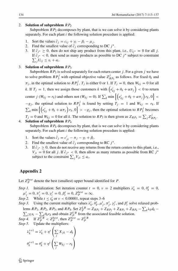
134 Jnl Remanufactur (2017) 7:113–137
2. Solution of subproblem RP2Subproblem RP2 decomposes by plant, that is we can solve it by considering plants
separately. For each plant i the following solution procedure is applied:
1. Sort the values cj = cij + γi − βi − μj .2. Find the smallest value of cj corresponding to DC j∗.3. If cj∗ ≥ 0, then do not ship any product from this plant, i.e., Uij∗ = 0 for all j.
If cj∗ < 0, then send as many products as possible to DC j∗ subject to constraint∑jUij ≤ si + ai .
3. Solution of subproblem RP3Subproblem RP3 is solved separately for each return center j . For a given j we have
to solve problem RPj
3 with optimal objective value ZjRP3
as follows. For fixed θk and
πj , in the optimal solution to RPj
3 , Tj is either 0 or 1. If Tj = 0, then Wkj = 0 for all
k. If Tj = 1, then we assign those customers k with(e′kj + θk + απj
)< 0 to return
center j (Wkj = rk) and others not (Wkj = 0). If∑
k min{(
e′kj + θk + απj
)rk, 0
}<
−gj , the optimal solution to RPj
3 is found by setting Tj = 1 and Wkj = rk . If∑k min
{(e′kj + θk + απj
)rk, 0
}> −gj , then the optimal solution to RP
j
3 becomes
Tj = 0 and Wkj = 0 for all k. The solution to RP3 is then given as ZRP3 = ∑jZ
jRP3
.4. Solution of subproblem RP4
Subproblem RP4 decomposes by plant, that is we can solve it by considering plantsseparately. For each plant i the following solution procedure is applied:
1. Sort the values cj = c′ji − πj − γi + βi.
2. Find the smallest value of cj corresponding to RC j∗.3. If cj∗ ≥ 0, then do not receive any returns from the return centers to this plant, i.e.,
Vji = 0 for all j . If cj∗ < 0, then allow as many returns as possible from RC j∗subject to the constraint
∑jVji ≤ ai .
Appendix 2
Let ZbestP denote the best (smallest) upper bound identified for P .
Step 1. Initialization: Set iteration counter t = 0, ν = 2 multipliers λtk = 0, θ t
k = 0,μt
j = 0, πtj = 0, γ t
i = 0, βti = 0, Zbest
P = ∞.Step 2. While t ≤ t ′0 or ν < 0.00001, repeat steps 3–6Step 3. Using the current multiplier values λt
k , θ tk , μt
j , πtj , γ t
i , and βti solve relaxed prob-
lems RP1, RP2, RP3, and RP4. Set ZLBP = ZRP1 + ZRP2 + ZRP3 + ZRP4 −∑kλkdk −∑
iγisi −∑kθkrk and obtain ZUB
P from the associated feasible solution.Step 4. If ZUB
P < ZbestP , then Zbest
P = ZUBP
Step 5. Update the multipliers:
λt+1k = λt
k + ηt
(∑j
Xjk − dk
)
θ t+1k = θ t
k + ηt
(∑j
Wkj − rk
)

Jnl Remanufactur (2017) 7:113–137 135
μt+1j = μt
j + ηt
(∑k
Xjk −∑i
Uij
)
πt+1j = πt
j + ηt
(α∑k
Wkj −∑i
Vji
)
γ t+1i = max
{0, γ t
i + ηt
(∑j
Uij −∑j
Vji − si
)}and
βt+1i = max
{0, βt
i + ηt
(∑j
Vji −∑j
Uij
)}.
In the above equations, ηt is the step size given as
ηt = ν(Zbest
P − ZLBP
)Denom
(14)
where
Denom =∑
k
⎡⎢⎣⎛⎝∑
j
Xjk − dk
⎞⎠
2
+⎛⎝∑
j
Wkj − rk
⎞⎠
2⎤⎥⎦
+∑j
⎡⎣(∑
k
Xjk −∑
i
Uij
)2
+(
α∑
k
Wkj −∑
i
Vji
)2⎤⎦
+∑
i
⎡⎢⎣⎛⎝∑
j
Uij −∑j
Vji − si
⎞⎠
2
+⎛⎝∑
j
Vji −∑j
Uij
⎞⎠
2⎤⎥⎦
Step 6. Set ν = ν/2 if there is no improvement in the lower bound for the last 30 iterations.In order to determine the step size for updating the multipliers as in (14), we need an
upper bound ZUBP to problem P as well as the associated Uij and Vji values which are
feasible to problem RP .
References
1. Agrawal S, Singh RK, Murtaza Q (2015) A literature review and perspectives in reverse logistics. ResourConserv Recycl 97:76–92
2. Amin SH, Baki F (2017) A facility location model for global closed-loop supply chain network design.Appl Math Model 41:316–330
3. Amin SH, Zhang G (2013) A multi-objective facility location model for closed-loop supply chainnetwork under uncertain demand and return. Appl Math Model 37(6):4165–4176
4. Aras N, Boyacı T, Verter V (2004) The effect of categorizing returned products in re-manufacturing. IIETrans 36:319–331
5. Beamon BM, Fernandes C (2004) Supply-chain network configuration for product recovery. Prod PlanControl 15(3):270–281
6. Chen W, Kucukyazici B, Verter V, Saenz MJ (2015) Supply chain design for unlocking the value ofremanufacturing under uncertainty. Eur J Oper Res 247:804–819
7. Chen YT, Chan FTS, Chung SH (2015) An integrated closed-loop supply chain model with locationallocation problem and product recycling decisions. Int J Prod Res 53(10):3120–3140
8. Demirel NO, Gokcen H (2008) A Mixed-Integer programming model for remanufacturing in reverselogistics environment. Int J Adv Manuf Tech 39(11–12):1197–1206

136 Jnl Remanufactur (2017) 7:113–137
9. Demirel N, Ozceylan E, Paksoy T, Gokcen H (2014) A genetic algorithm approach for optimisinga closed-loop supply chain network with crisp and fuzzy objectives. Int J Prod Res 52(12):3637–3664
10. Easwaran G, Uster H (2010) A Closed-Loop supply chain network design problem with integratedforward and reverse channel decisions. IIE Trans 42(11):779–792
11. Fleischmann M, Krikke HR, Dekker R, Flapper SDP (2000) A characterization of logistics networks forproduct recovery. Omega 28:653–666
12. Fleischmann M, Beullens P, Bloemhof-Ruwaard JM, Van Wassenhove LN (2001) The impact of productrecovery on logistics network design. Prod Oper Manag 10:156–173
13. Govindan K, Soleimani H, Kannan D (2015) Reverse logistics and closed-loop supply chain: acomprehensive review to explore the future. Eur J Oper Res 240:603–626
14. HP (2017) Recycling program overview. http://www8.hp.com/us/en/hp-information/environment/product-recycling.html. (Accessed 29 March 2017)
15. Keyvanshokooh E, Fattahi M, Syed-Hosseini SM, Tavakkoli-Moghaddam R (2013) A dynamic pric-ing approach for returned products in integrated Forward/Reverse logistics network design. Appl MathModel 37:10182–10202
16. Ko HJ, Evans GW (2007) A genetic-based heuristic for the dynamic integrated Forward/Reverse logisticsnetwork for 3PLs. Comput Oper Res 34(2):346–366
17. Krikke HR, Bloemhof-Ruwaard JM, Van Wassenhove LN (2003) Concurrent product and closed-Loopsuplly chain design with an application to refrigerators. Int J Prod Res 41(16):3689–3719
18. Lee D-H, Dong M (2008) A heuristic approach to logistics network design for end-of-lease computerproducts recovery. Transport Res E-Log 44(3):455–474
19. Lee D-H, Dong M (2009) Dynamic network design for reverse logistics operations under uncertainty.Transport Res E-Log 45:61–71
20. Listes O (2007) A generic stochastic model for supply-and-return network design. Comput Oper Res34(2):417–442
21. Lu Z, Bostel N (2007) A facility location model for logistics systems including reverse flows: The caseof remanufacturing activities. Comput Oper Res 34(2):299–323
22. Marın A, Pelegrin B (1998) The return plant location problem: Modelling and resolution. Eur J OperRes 104(2):375–392
23. Ozkır V, Baslıgil H (2012) Modelling product-recovery processes in closed-loop supply-chain networkdesign. Int J Prod Res 50(18):2218–2233
24. Pedram A, Bin Yusoff N, Udoncy OE, Mahat AB, Pedram P, Babalola A (2017) Integrated forward andreverse supply chain: a tire case study. Waste Manage 60:460–470
25. Pishvaee MS, Jolai F, Razmi J (2009) A stochastic optimization model for integrated Forward/Reverselogistics network design. J Manuf Syst 28(4):107–114
26. Pishvaee MS, Farahani RZ, Dullaert W (2010) A memetic algorithm for bi-objective forward-reverselogistics network design. Comput Oper Res 37(6):1100–1123
27. Rosa VD, Gebhard M, Hartmann E, Wollenweber J (2013) Robust sustainable bi-directional logisticsnetwork design under uncertainty. Int J Prod Econ 145:184–198
28. Sahyouni K, Savaskan C, Daskin M (2007) A facility location model for bidirectional flows. TransportSci 41(4):484–499
29. Salema MI, Barbosa-Povoa AP, Novais AQ (2006) A warehouse-based design model for reverselogistics. J Oper Res Soc 57(6):615–629
30. Salema MI, Barbosa-Povoa AP, Novais AQ (2007) An optimization model for the design of a capacitatedmulti-product reverse logistics network with uncertainty. Eur J Oper Res 179(3):1063–1077
31. Salema MI, Povoa APB, Novais AQ (2009) A strategic and tactical model for closed-loop supply chains.OR Spectrum 31(3):573–599
32. Salema MIG, Barbosa-Povoa PB, Novais AQ (2010) Simultaneous design and planning of supply chainswith reverse flows simultaneous a generic modelling framework. Eur J Oper Res 203(2):336–349
33. Shi J, Liu Z, Tang L, Xiong J (2017) Multi-objective optimization for a closed-loop network designproblem using an improved genetic algorithm. Appl Math Model 45:14–30
34. Remanufactured Goods (2012) An Overview of the U.S. and Global Industries, Markets, and Trade.Investigation No. 332-525, U.S. International Trade Commission. https://www.usitc.gov/publications/332/pub4356.pdf (Accessed 29 March 2017)
35. Uster H, Easwaran G, Akcalı E, Cetinkaya S (2007) Benders decomposition with alternative multiplecuts for a multi-product closed-loop supply chain network design model. Nav Res Log 54:890–907
36. WEEE Directive 2012/19/EU of directive of the European parliament and council on waste electri-cal and electrical equipment. http://ec.europa.eu/environment/waste/weee/index en.htm. (Accessed 29March 2017)
Jnl Remanufactur (2017) 7:113–137 137
37. Xerox (2014) Report on global citizenship https://www.xerox.com/corporate-citizenship/2014/sustainability/sustainable-products/enus.html. (Accessed 29 March 2017)
38. Wang HF, Hsu HW (2010) A closed-loop logistic model with a spanning-tree based genetic algorithm.Comput Oper Res 37(2):376–389
39. Zhang J, Liu X, Tu YL (2011) A capacitated production planning problem for closed-loop supply chainwith remanufacturing. Int J Adv Manuf Technol 54:757–766
40. Zhou Y, Wang S (2008) Generic model of reverse logistics network design. J Transp Syst Eng InfTechnol 8(3):71–78