1

Designing Intelligent Tutors That Adapt to When Students Game the System

Ryan Shaun Baker December, 2005

Doctoral Dissertation Human-Computer Interaction Institute

School of Computer Science Carnegie Mellon University

Pittsburgh, PA USA

Carnegie Mellon University, School of Computer Science Technical Report CMU-HCII-05-104

Thesis Committee:

Albert T. Corbett, co-chair Kenneth R. Koedinger, co-chair

Shelley Evenson Tom Mitchell

Submitted in partial fulfillment of the requirements for the degree of Doctor of Philosophy

Copyright © 2005 by Ryan Baker. All rights reserved.

This research was sponsored in part by an NDSEG (National Defense Science and Engineering Graduate) Fellowship, and by National Science Foundation grant REC-043779. The views and conclusions contained in this document are those of the author and should not be interpreted as representing the official policies or endorsement, either express or implied, of the NSF, the ASEE, or the U.S. Government.

2

Keywords: intelligent tutoring systems, educational data mining, human-computer interaction, gaming the system, quantitative field observations, Latent Response Models, intelligent agents

3

Abstract

Students use intelligent tutors and other types of interactive learning environments in a considerable variety of ways. In this thesis, I detail my work to understand, automatically detect, and re-design an intelligent tutoring system to adapt to a behavior I term “gaming the system”. Students who game the system attempt to succeed in the learning environment by exploiting properties of the system rather than by learning the material and trying to use that knowledge to answer correctly. Within this thesis, I present a set of studies aimed towards understanding what effects gaming has on learning, and why students game, using a combination of quantitative classroom observations and machine learning. In the course of these studies, I determine that gaming the system is replicably associated with low learning. I use data from these studies to develop a profile of students who game, showing that gaming students have a consistent pattern of negative affect towards many aspects of their classroom experience and studies. Another part of this thesis is the development and training of a detector that reliably detects gaming, in order to drive adaptive support. In this thesis, I validate that this detector transfers effectively between 4 different lessons within the middle school mathematics tutor curriculum without re-training, suggesting that it may be immediately deployable to that entire curriculum. Developing this detector required developing new machine learning methods that effectively combine unlabeled data and labeled data at different-grain sizes in order to train a model to accurately indicate both which students were gaming, and when they were gaming. To this end, I adapted a modeling framework from the Psychometrics literature – Latent Response Models (Maris, 1995), and used a variant of Fast Correlation-Based Filtering (Yu and Liu 2003) to efficiently search the space of potential models. The final part of this thesis is the re-design of an existing intelligent tutoring lesson to adapt to gaming. The re-designed lesson incorporates an animated agent (“Scooter the Tutor”) who indicates to the student and their teacher whether the student has been gaming recently. Scooter also gives students supplemental exercises, in order to offer the student a second chance to learn the material he/she had gamed through. Scooter reduces the frequency of gaming by over half, and Scooter’s supplementary exercises are associated with substantially better learning; Scooter appears to have had virtually no effect on the other students.

4

Acknowledgements

The list of people that I should thank for their help and support in completing this dissertation would fill an entire book. Here, instead, is an incomplete list of some of the people I would like to thank for their help, support, and suggestions. Angela Wagner, Ido Roll, Mike Schneider, Steve Ritter, Tom McGinnis, and Jane Kamneva assisted in essential ways with the implementation and administration of the studies presented in this dissertation. None of the studies presented here could have occurred without the support of Jay Raspat, Meghan Naim, Dina Crimone, Russ Hall, Sue Cameron, Frances Battaglia, and Katy Getman, in welcoming me into their classrooms. The ideas presented in this dissertation were refined through conversations with Ido Roll, Santosh Mathan, Neil Heffernan, Aatish Salvi, Dan Baker, Cristen Torrey, Darren Gergle, Irina Shklovski, Peter Scupelli, Aaron Bauer, Brian Junker, Joseph Beck, Jack Mostow, Carl diSalvo, and Vincent Aleven. My committee members, Shelley Evenson and Tom Mitchell, helped to shape this dissertation into its present form, teaching me a great deal about design and machine learning in the process. My advisors, Albert Corbett and Kenneth Koedinger, were exceptional mentors, and have guided me for the last five years in learning how to conduct research effectively, usefully, and ethically – I owe an immeasurable debt to them. Finally, I would like to thank my parents, Sam and Carol, and my wife, Adriana. Their support guided me when the light at the end of the dissertation seemed far.

5

Table of Contents I II III IV V VI

Introduction Gaming the System and Learning Detecting Gaming Understanding Why Students Game Adapting to Gaming Conclusions and Future Work References

7 12 21 41 54 79 83

Appendices A B C

Cognitive Tutor Lessons Learning Assessments Gaming Detectors

87 94 108

6

Chapter One Introduction

In the last twenty years, interactive learning environments and computerized educational supports have become a ubiquitous part of students’ classroom experiences, in the United States and throughout the world. Many such systems have become very effective at assessing and responding to differences in student knowledge and cognition (Corbett and Anderson 1995; Martin and vanLehn 1995; Arroyo, Murray, Woolf, and Beal 2003; Biswas et al 2005). Systems which can effectively assess and respond to cognitive differences have been shown to produce substantial – and statistically significant – learning gains, as compared to students in traditional classes (cf. Koedinger, Anderson, Hadley, and Mark 1997; vanLehn et al 2005). However, even within classes using interactive learning environments which have been shown to be effective, there is still considerable variation in student learning outcomes, even when each student’s prior knowledge is taken into account. The thesis of this dissertation is that a considerable amount of this variation comes from differences in how students choose to use educational software, that we can determine which behaviors are associated with poorer learning, and that we can develop systems that can automatically detect and respond to those behaviors, in a fashion that improves student learning. In this dissertation, I present results showing that one way that students use educational software, gaming the system, is associated with substantially poorer learning – much more so, in fact, than if the student spent a substantial portion of each class ignoring the software and talking off-task with other students (Chapter 2). I then develop a model which can reliably detect when a student is gaming the system, across several different lessons from a single Cognitive Tutor curriculum (Chapter 3). Using a combination of the gaming detector and attitudinal questionnaires, I compile a profile of the prototypical gaming student, showing that gaming students differ from other students in several respects (Chapter 4). I next combine the gaming detector and profile of gaming students, in order to re-design existing Cognitive Tutor lessons to address gaming. My re-design introduces an interactive agent, Scooter the Tutor, who signals to students (and their teachers) that he knows that the student is gaming, and gives supplemental exercises targeted towards the material students are missing by gaming (Chapter 5). Scooter substantially decreases the incidence of gaming, and his exercises are associated with substantially better learning. In Chapter 6, I discuss the larger implications of this dissertation, advancing the idea of interactive learning environments that effectively adapt not just to differences in student cognition, but differences in student choices.

Gaming the System I define “Gaming the System” as attempting to succeed in an educational environment by exploiting properties of the system rather than by learning the material and trying to use that knowledge to answer correctly. Gaming strategies are seen by teachers and outsiders as misuse of the software the student is using or system that the student is participating in, but are distinguished from cheating in that gaming does not violate explicit rules of the educational setting, as cheating does. In fact, in some situations students are encouraged to game the system – for instance, several test preparation companies teach students to use the structure of how SAT

7

questions are designed in order to have a higher probability of guessing the correct answer. Cheating on the SAT, by contrast, is not recommended by test preparation companies. Gaming the System occurs in a wide variety of different educational settings, both computerized and offline. To cite just a few examples: Arbreton (1998) found that students ask teachers or teachers’ aides to give them answers to math problems before attempting the problems themselves. Magnussen and Misfeldt (2004) have found that students take turns intentionally making errors in collaborative educational games in order to help their teammates obtain higher scores; gaming the system has also been documented in other types of educational games (Klawe 1998; Miller, Lehman, and Koedinger 1999). Cheng and Vassileva (2005) have found that students post irrelevant information – in large quantities – to newsgroups in online courses which are graded based on participation. Within intelligent tutoring systems, gaming the system has been particularly well-documented. Schofield (1995) found that some students quickly learned to ask for the answer within a prototype intelligent tutoring system which did not penalize help requests, instead of attempting to solve the problem on their own – a behavior quite similar to that observed by Arbreton (1998). Wood and Wood (1999) found that students quickly and repeatedly ask for help until the tutor gives the student the correct answer, a finding replicated by Aleven and Koedinger (2000). Mostow and his colleagues (2002) found in a reading tutor that students often avoid difficulty by re-reading the same story over and over. Aleven and his colleagues (1998) found, in a geometry tutor, that students learn what answers are most likely to be correct (such as numbers in the givens, or 90 or 180 minus one of those numbers), and try those numbers before thinking through a problem. Murray and vanLehn (2005) found that students using systems with delayed hints (a design adopted by both Carnegie Learning (Aleven 2001) and by the AnimalWatch project (Beck 2005) as a response to gaming) intentionally make errors at high speed in order to activate the software’s proactive help. Within the intelligent tutoring systems we studied, we primarily observed two types of gaming the system:

1. quickly and repeatedly asking for help until the tutor gives the student the correct answer (as in Wood and Wood 1999; Aleven and Koedinger 2000)

2. inputting answers quickly and systematically. For instance, entering 1,2,3,4,… or clicking every checkbox within a set of multiple-choice answers, until the tutor identifies a correct answer and allows the student to advance.

In both of these cases, features designed to help a student learn curricular material via problem-solving were instead used by some students to solve the current problem and move forward within the curriculum.

The Cognitive Tutor Classroom All of the studies that I will present in this dissertation took place in classes using Cognitive Tutor software (Koedinger, Anderson, Hadley, and Mark 1995). In these classes, students complete mathematics problems within the Cognitive Tutor environment. The problems are designed so as to reify student knowledge, making student thinking (and misconceptions) visible. A running cognitive model assesses whether the student’s answers map to correct understanding

8

or to a known misconception. If the student’s answer is incorrect, the answer turns red; if the student’s answers are indicative of a known misconception, the student is given a “buggy message” indicating how their current knowledge differs from correct understanding (see Figure 1-1). Cognitive Tutors also have multi-step hint features; a student who is struggling can ask for a hint. He or she first receives a conceptual hint, and can request further hints, which become more and more specific until the student is given the answer (see Figure 1-2). Students in the classes studied used the Cognitive Tutor 2 out of every 5 or 6 class days, devoting the remaining days to traditional classroom lectures and group work. In Cognitive Tutor classes, conceptual instruction is generally given through traditional classroom lectures – however, in order to guarantee that all students had the same conceptual instruction in our studies, we used PowerPoint presentations with voiceover and simple animations to deliver conceptual instruction (see Figure 1-3). The research presented in this dissertation was conducted in classrooms using a new Cognitive Tutor curriculum for middle school mathematics (Koedinger 2002), in two suburban school districts near Pittsburgh. The students participating in these studies were in the 7th-9th grades (predominantly 12-14 years old). In order to guarantee that students were familiar with the Cognitive Tutor curriculum, and how to use the tutors (and – presumably – how to game the system if they wanted to), all studies were conducted in the Spring semester, after students had already been using the tutors for several months.

Figure 1-1: The student has made an error associated with a misconception, so they receive a “buggy message” (top window). The student’s answer is labeled in red, because it is incorrect (bottom window).

9

Figure 1-2: The last stage of a multi-stage hint: The student labels the graph’s axes and plots points in the left window; the tutor’s estimates of the student’s skills are shown in the right window; the hint window (superimposed on the left window) allows the tutor to give the student feedback. Other windows (such as the problem scenario and interpretation questions window) are not shown.

Figure 1-3: Conceptual instruction was given via PowerPoint with voice-over,

in the studies presented within this dissertation.

Effectiveness of Existing Cognitive Tutors It is important, before discussing how some students succeed less well in Cognitive Tutors than others, to remember that Cognitive Tutors are an exceptionally educationally effective type of learning environment overall. Cognitive Tutors have been validated to be highly effective across a wide variety of educational domains and studies. To give a few examples, a Cognitive Tutor for the LISP programming language achieved a learning gain almost two standard deviations better than an unintelligent interactive learning environment (Corbett 2001); a Cognitive Tutor for Geometry proofs resulted in test scores a letter grade higher than students learning about Geometry proofs in a traditional classroom (Anderson, Corbett, Koedinger, and Pelletier 1995); and an Algebra Cognitive Tutor has shown in a number of studies conducted nationwide to not only lead to better scores on the Math SAT standardized test than traditional curricula

10

(Koedinger, Anderson, Hadley, and Mark 1997), but to also result in a higher percentage of students choosing to take upper-level mathematics courses (Carnegie Learning 2005). In recent years, the Cognitive Tutor curricula have come into use in an increasing percentage of U.S. high schools – about 6% of U.S. high schools as of the 2004-2005 school year. Hence, the goal of the research presented here is not to downgrade in any way the effectiveness of Cognitive Tutors. Cognitive Tutors are one of the most effective types of curricula in existence today, across several types of subject matter. Instead, within this dissertation I will attempt to identify a direction that may make Cognitive Tutors even better. A majority of students use Cognitive Tutors thoughtfully, and have excellent learning gains; a minority, however, use tutors less effectively, and learn less well. The goal of the research presented here is to improve the tutors for the students who are less well-served by existing tutoring systems, while minimally affecting the learning experience of students who already use tutors appropriately. It is worth remembering that students game the system in a variety of different types of learning environments, not just in Cognitive Tutors. Though I do not directly address how gaming affects student learning in these systems, or how these systems should adapt to gaming, it will be a valuable area of future research to determine how this thesis’s findings transfer from cognitive tutors to other types of interactive learning environments.

Studies

The work reported in this thesis is composed of three classroom studies, multiple iterations of the development of a system to automatically detect gaming, analytic work, and the design and implementation of a system to adapt to when students game. The first study (“Study One”) took place in the Spring of 2003. In Study One, I combined data from human observations and pre-test/post-test scores, to determine what student behaviors are most associated with poorer learning, finding that gaming the system is particularly associated with poorer learning (Chapter 2). Data from this study was used to create the first gaming detector (Chapter 3); in developing the gaming detector, I determined that gaming split into two automatically distinguishable categories of behavior, associated with different learning outcomes (Chapter 3). Data from Study One was also useful for developing first hypotheses as to what characteristics and attitudes were associated with gaming (Chapter 4). The second study (“Study Two”) took place in the Spring of 2004. In Study Two, I analyzed what student characteristics and attitudes are associated with gaming (Chapter 4). I also replicated our earlier result that gaming is associated with poorer learning (Chapter 2), and demonstrated that our human observations of gaming had good inter-rater reliability (Chapter 2). Data from Study Two was also used to refine our detector of gaming (Chapter 3). The third study (“Study Three”) took place in the Spring of 2005. In Study Three, I deployed a re-designed tutor lesson that incorporated an interactive agent designed to both reduce gaming and mitigate its effects (Chapter 5). I also gathered further data on which student characteristics and attitudes are associated with gaming (Chapter 4), using this data in combination with data from Study Two to develop a profile of gaming students (Chapter 4). Finally, Data from Study Three was used in a final iteration of gaming detector improvement (Chapter 3).

11

Chapter Two Gaming the System and Learning

In this chapter, I will present two studies which provide evidence on the relationship between gaming the system and learning. Along the way, I will present a method for collecting quantitative observations of student behavior as they use intelligent learning environments in class, adapted from methods used in the off-task behavior and behavior modification literatures, and consider how this method’s effectiveness can be amplified with machine learning.

Study One By 2003 (when the first study reported in this dissertation was conducted), gaming had been repeatedly documented, and had inspired the re-design of intelligent tutoring systems both at Carnegie Mellon University/Carnegie Learning (documented later in Aleven 2001, and Murray and vanLehn 2005) and at the University of Massachusetts (documented later in Beck 2005). Despite this, there was not yet any published evidence that gaming was associated with poorer learning. In Study One, I investigate what learning outcomes are associated with gaming, comparing these outcomes to the learning outcomes associated with other behaviors. In particular, I compare the hypothesis that gaming will be specifically associated with poorer learning, to Carroll’s Time-On-Task hypothesis (Carroll 1963; Bloom 1976). Under Carroll’s Time-On-Task hypothesis, the longer a student spends engaging with the learning materials, the more opportunities the student has to learn. Therefore, if a student spends a greater fraction of their time off-task (engaged in behaviors where learning from the material is not the primary goal)1, they will spend less time on-task, and learn less. If the Time-On-Task hypothesis were the main reason why off-task behavior reduces learning, then any type of off-task behavior, including talking to a neighbor or surfing the web, should have the same (negative) effect on learning as gaming does. Methods I studied the relationship between gaming and learning in a set of 5 middle-school classrooms at 2 schools in the Pittsburgh suburbs. Student ages ranged from approximately 12 to 14. As discussed in Chapter 1, the classrooms studied were taking part in the development of a new 3-year Cognitive Tutor curriculum for middle school mathematics. Seventy students were present for all phases of the study (other students, absent during one or more days of the study, were excluded from analysis).

1 It is possible to define on-task as “looking at the screen”, in which case gaming the system is viewed as an on-task behavior. Of course, the definition of “on-task” depends on what one considers the student’s task to be – I do not consider just “looking at the screen” to be that task.

12

I studied these classrooms during the course of a short (2 class period) Cognitive Tutor lesson on scatterplot generation and interpretation – this lesson is discussed in detail in Appendix A. The day before students used the tutoring software, they viewed a PowerPoint presentation giving conceptual instruction (shown in Chapter 1). I collected the following sources of data to investigate gaming’s relationship to learning: A pre-test and post-test to assess student learning, quantitative field observations to assess each student’s frequency of different behaviors, students’ end-of-course test scores (which incorporated both

multiple-choice and problem-solving exercises) as a measure of general academic achievement2. We also noted each student’s gender, and collected detailed log files of the students’ usage of the Cognitive Tutoring software. The pre-test was given after the student had finished viewing the PowerPoint presentation, in order to study the effect of the Cognitive Tutor rather than studying the combined effect of the declarative instruction and Cognitive Tutor. The post-test was given at the completion of the tutor lesson. The pre-test and post-test were drawn from prior research into tutor design in the tutor’s domain area (scatterplots), and are discussed in detail in Appendix B. The quantitative field observations were conducted as follows: Each student’s behavior was observed a number of times during the course of each class period, by one of two observers. I chose to use outside observations of behavior rather than self-report in order to interfere minimally with the experience of using the tutor – I was concerned that repeatedly halting the student during tutor usage to answer a questionnaire (which was done to assess motivation by deVicente and Pain (2002)) might affect both learning and on/off-task behavior. In order to investigate the relative impact of gaming the system as compared to other types of off-task behavior, the two observers coded not just the frequency of off-task behavior, but its nature as well. This method differs from most past observational studies of on and off-task behavior, where the observer coded only whether a given student was on-task or off-task (Lahaderne 1968; Karweit and Slavin 1982; Lloyd and Loper 1986; Lee, Kelly, and Nyre 1999). The coding scheme consisted of six categories:

1. on-task -- working on the tutor

2. on-task conversation -- talking to the teacher or another student about the subject material

3. off-task conversation – talking about anything other than the subject material

4. off-task solitary behavior – any behavior that did not involve the tutoring software or another individual (such as reading a magazine or surfing the web)

5. inactivity -- for instance, the student staring into space or putting his/her head down on the desk for the entire 20-second observation period

6. gaming the system – inputting answers quickly and systematically, and/or quickly and repeatedly asking for help until the tutor gives the student the correct answer

2 We were not able to obtain end-of-course test data for one class, due to that class’s teacher accidentally discarding the sheet linking students to code numbers.

13

In order to avoid bias towards more interesting or dramatic events, the coder observed the set of students in a specific order determined before the class began, as in Lloyd and Loper (1986). Any behavior by a student other than the student currently being observed was not coded. A total of 563 observations were taken (an average of 70.4 per class session), with an average of 8.0 observations per student, with some variation due to different class sizes and students arriving to class early or leaving late. Each observation lasted for 20 seconds – if a student was inactive for the entire 20 seconds, the student was coded as being inactive. If two distinct behaviors were seen during an observation, only the first behavior observed was coded. In order to avoid affecting the current student’s behavior if they became aware they were being observed, the observer viewed the student out of peripheral vision while appearing to look at another student. In practice, students became comfortable with the presence of the observers very quickly, as evinced by the fact that we saw students engaging in the entire range of studied behaviors. The two observers observed one practice class period together before the study began. In order to avoid alerting a student that he or she was currently being observed, the observers did not observe any student at the same time. Hence, for this study, we cannot compare the two observers’ assessment of the exact same time-slice of a student’s behavior, and thus cannot directly compute a traditional measure of inter-rater reliability. The two observers did conduct simultaneous observations in Study Two, and I will present an inter-rater reliability measure for that study. Results

Overall Results The tutor was, in general, successful. Students went from 40% on the pre-test to 71% on the post-test, which was a significant improvement, F(1,68)=7.59, p<0.01. Knowing that the tutor was overall successful is important, since it establishes that a substantial number of students learned from the tutor; hence, we can investigate what characterizes the students who learned less. Students were on-task 82% of the time, which is within the previously reported ranges for average classes utilizing traditional classroom instruction (Lloyd and Loper 1986; Lee, Kelly, and Nyre 1999). Within the 82% of time spent on-task, 4% was spent talking with the teacher or another student, while the other 78% was solitary. The most frequent off-task behavior was off-task conversation (11%), followed by inactivity (3%), and off-task solitary behavior (1%). Students gamed 3% of the time – thus, gaming was substantially less common than off-task conversation, but occurred a proportion of the time comparable to inactivity. More students engaged in these behaviors than the absolute frequencies might suggest: 41% of the students were observed engaging in off-task conversation at least once, 24% were observed gaming the system at least once, 21% were observed to be inactive at least once, and 9% were observed engaging in off-task solitary behavior at least once. 100% of the students were observed working at least once. A student’s prior knowledge of the domain (measured by the pre-test) was a reasonably good predictor of their post-test score, F(1,68)=7.59, p<0.01, r=0.32. A student’s general level of academic achievement was also a reasonably good predictor of the student’s post-test score, F(1,61)=9.31, p<0.01, r=0.36. Prior knowledge and the general level of academic achievement were highly correlated, F(1,61)=36.88, p<0.001, r=0.61; when these two terms were both used as predictors, the correlation between a student’s general level of academic achievement and their post-test score was no longer significant, F(1,60)=1.89, p=0.17.

14

Gender was not predictive of post-test performance, F(1,68)=0.42, p=0.52. Neither was which teacher the student had, F(3,66)=0.5,p=0.69. Gaming the System and Off-Task Behavior: Relationships to Learning Only two types of behavior were found to be significantly negatively correlated with the post-test, as shown in Table 2-1.

Prior Knowledge (Pre-Test)

General Academic

Achievement

Gaming the System

Talking Off-Task

Inactivity

Off-Task Solitary Behavior

Talking On-Task

Gender Teacher

Post-Test

0.32 0.36 -0.38 -0.19 -0.08 -0.08 -0.24 -0.08 n/a, n/s

Table 2-1: The correlations between post-test score and the other measures in Study One. Statistically significant relationships are in boldface

The behavior most negatively correlated with post-test score was gaming the system. The frequency of gaming the system was the only off-task behavior which was significantly correlated with the post-test, F(1,68)=11.82, p<0.01, r= -0.38. The impact of gaming the system remains significant even when we control for the students’ pre-test and general academic achievement, F(1,59)=7.73, p<0.01, partial correlation = -0.34. No other off-task behavior was significantly correlated with post-test score. The closest was the frequency of talking off-task, which was at best marginally significantly correlated with post-test score, F(1,68)=2.45, p=0.12, r= -0.19. That relationship reduced to F(1,59)=2.03, p=0.16, partial correlation r=-0.22, when we controlled for pre-test and general academic achievement. Furthermore, the frequencies of inactivity (F(1,68)=0.44, p=0.51, r=-0.08) and off-task solitary behavior (F(1,68)=0.42, p=0.52,r=-0.08) were not significantly correlated to post-test scores. Unexpectedly, however, the frequency of talking to the teacher or another student about the subject matter was significantly negatively correlated to post-test score, F(1,68)=4.11, p=0.05, r= -0.24, and this remained significant even when we controlled for the students’ pre-test and general academic achievement, F(1,59)=3.88, p=0.05, partial correlation = -0.25. As it turns out, students who talk on-task also game the system, F(1,68)=10.52,p<0.01, r=0.37. This relationship remained after controlling for prior knowledge and general academic achievement, F(1,59) = 8.90, p<0.01, partial correlation = 0.36. The implications of this finding will be discussed in more detail in Chapter Four, when we discuss why students game the system. To put the relationship between the frequency of gaming the system and post-test score into better context, we can compare the post-test scores of students who gamed with different frequencies. Using the median frequency of gaming among students who ever gamed (gaming 10% of the time), we split the 17 students who ever gamed into a high-gaming half (8 students) and a low-gaming half (9 students). We can then compare the 8 high-gaming students to the 53 never-gaming students. The 8 high-gaming students’ mean score at post-test was 44%, which was significantly lower than the never-gaming students’ mean post-score of 78%, F(1,59)=8.61, p<0.01. However, the 8 high-gaming students also had lower pre-tests. The 8 high-gaming students had an average pre-test score of 8%, with none scoring over 17%, while the 53 never-gaming students averaged 49% on the pre-test. Given this, one might hypothesize that choosing

15

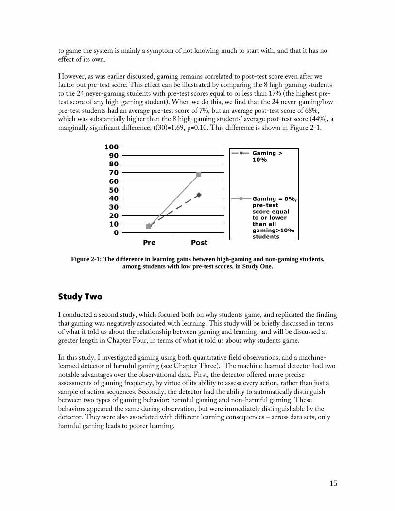
to game the system is mainly a symptom of not knowing much to start with, and that it has no effect of its own. However, as was earlier discussed, gaming remains correlated to post-test score even after we factor out pre-test score. This effect can be illustrated by comparing the 8 high-gaming students to the 24 never-gaming students with pre-test scores equal to or less than 17% (the highest pre-test score of any high-gaming student). When we do this, we find that the 24 never-gaming/low-pre-test students had an average pre-test score of 7%, but an average post-test score of 68%, which was substantially higher than the 8 high-gaming students’ average post-test score (44%), a marginally significant difference, t(30)=1.69, p=0.10. This difference is shown in Figure 2-1.

Figure 2-1: The difference in learning gains between high-gaming and non-gaming students, among students with low pre-test scores, in Study One.

Study Two I conducted a second study, which focused both on why students game, and replicated the finding that gaming was negatively associated with learning. This study will be briefly discussed in terms of what it told us about the relationship between gaming and learning, and will be discussed at greater length in Chapter Four, in terms of what it told us about why students game. In this study, I investigated gaming using both quantitative field observations, and a machine-learned detector of harmful gaming (see Chapter Three). The machine-learned detector had two notable advantages over the observational data. First, the detector offered more precise assessments of gaming frequency, by virtue of its ability to assess every action, rather than just a sample of action sequences. Secondly, the detector had the ability to automatically distinguish between two types of gaming behavior: harmful gaming and non-harmful gaming. These behaviors appeared the same during observation, but were immediately distinguishable by the detector. They were also associated with different learning consequences – across data sets, only harmful gaming leads to poorer learning.

�

��

��

��

��

��

��

��

�

�

���

�� ����

�����������

�������������� �� ������ � � �!������!�" ��#����!!������������ $ ���

16

Methods Study Two took place within 6 middle-school classrooms at 2 schools in the Pittsburgh suburbs. Student ages ranged from approximately 12 to 14. As discussed in Chapter One, the classrooms studied were taking part in the development of a new 3-year Cognitive Tutor curriculum for middle school mathematics. 102 students were present for all phases of the study (other students, absent during one or more days of the study, were excluded from analysis). I studied these classrooms during the course of the same Cognitive Tutor lesson on scatterplot generation and interpretation used in Study One. The day before students used the tutoring software, they viewed a PowerPoint presentation giving conceptual instruction (shown in Chapter One). Within this study, I combined the following sources of data: a questionnaire on student motivations and beliefs (to be discussed in Chapter Four), logs of each student’s actions within the tutor (analyzed both in raw form, and through the gaming detector), and pre-test/post-test data. Quantitative field observations were also obtained, as in Study One, as both a measure of student gaming and in order to improve the gaming detector’s accuracy. Inter-Rater Reliability One important step that I was able to take in Study Two was conducting a full inter-rater reliability session. As discussed earlier in this chapter, in Study One, the two observers did not conduct simultaneous observation, for fear of alerting a student that he or she was currently being observed. However, the two observers found that after a short period of time, students seemed to be fairly comfortable with the their presence; hence, during Study Two, they conducted an inter-rater reliability session. In order to do this, the two observers observed the same student out of peripheral vision, but from different angles. The observers moved from left to right; the observer on the observed student’s left stood close behind the student to the left of the observed student, and the observer on the observed student’s right stood further back and further right, so that the two observers did not appear to hover around a single student. In this session to evaluate inter-rater reliability, the two observers agreed as to whether an action was an instance of gaming 96% of the time. Cohen’s (1960) κ was 0.83, indicating high reliability between these two observers. A third observer took a small number of observations in this study (8% of total observations), as well, on two days when multiple classes were occurring simultaneously, and one of the two primary observers was unable to conduct observations. Because this observer filled in on days when one of the two primary observers was unavailable, it was not possible to formally investigate inter-rater reliability for this observer; however, this observer was conceptually familiar with gaming, and was trained within a classroom by one of the two primary observers. Results As in Study One, a student’s off-task behavior, excluding gaming, was not significantly correlated to the student’s post-test (when controlling for pre-test), F(1,97)=1.12, p= 0.29, partial r = - 0.11. By contrast to Study One’s results, however, talking on-task to the teacher or other students was also not significantly correlated to post-test (controlling for pre-test), F(1,97)=0.80, p=0.37,

17

partial r = - 0.09 (I will discuss the links between talking on-task and gaming in Chapter Four). Furthermore, asking other students for the answers to specific exercises was not significantly correlated to post-test (controlling for pre-test), F(1,97)=0.52, p=0.61, partial r = 0.05. Surprisingly, however, in Study Two, a student’s frequency of observed gaming did not appear to be significantly correlated to the student’s post-test (when controlling for pre-test), F(1,97)=1.16, p= 0.28, partial r = 0.07. Moreover, whereas the percentage of students in Study One who gamed the system and had poor learning (low pre-test, low post-test) was more or less equal to the percentage of students who gamed the system but had a high post-test, in Study Two almost 5 times as many students gamed the system and had a high post-test as gamed the system and had poor learning. This difference in ratio between the two studies (shown in Table 2-2) was significant, χ2(1, N=64)=6.00, p=0.01. However, this result is explainable as simply a difference in the ratio of two types of gaming, rather than a difference in the relationship between gaming and learning. These two types of gaming, harmful gaming and non-harmful gaming, are immediately distinguishable by the machine learning approach discussed in Chapter Three. In brief, students who engage in harmful gaming game predominantly on the hardest steps, while students who engage in non-harmful gaming mostly game on the steps they already know – the evidence that these two types of gaming are separable will be discussed in greater detail in Chapter Three. According to detectors of each type of gaming (trained on just the data from Study One), over twice as many students engaged in non-harmful gaming than harmful gaming in Study Two. Harmful gaming, detected by the detector trained on data from Study One, was negatively correlated with post-test score in Study Two, when controlling for pre-test, F(1,97)=5.78, p=0.02, partial r= - 0.24. By contrast, non-harmful gaming, as detected by the detector, was not significantly correlated to post-test score in Study Two, when controlling for pre-test, F(1,97)=0.86, p=0.36, partial r = 0.08. The lack of significant correlation between observed gaming and learning in Study Two can thus be attributed entirely to the fact that our observations did not distinguish between two separable categories of behavior – harmful gaming and non-harmful gaming.

Study One

(observations) Study Two

(observations) Study Two (detector)

Gamed, had low post-test (Harmful gaming)

11% 7% 22%

Gamed, had high post-test (Non-harmful gaming)

13% 34% 50%

Table 2-2: What percentage of students were ever seen engaging in each type of gaming, in the data from Study One and Study Two

When we look at the specific students detected engaging in harmful gaming, we see a similar pattern to the one observed in Study One. Looking just within the students with low pre-test scores (17% or lower, as with Study One), we see in Figure 2-2 that students who gamed harmfully more than the median (among students ever assessed as gaming harmfully) had considerably worse post-test scores (27%) than the students who never gamed (59%), while having more-or-less equal pre-test scores (4.3% versus 4.2%). The difference in post-test scores

18

between these two groups is marginally significant, t(56)=1.78, p=0.08, and in the same direction as the this test in Study One.

Figure 2-2: The difference in learning gains between high-harmful-gaming and non-harmful-gaming students, among students with low pre-test scores, in Study Two.

Study Two also gave us considerable data as to why students game. These results will be discussed in Chapter Four.

Contributions My work to study the relationship between gaming and learning has produced two primary contributions. The first contribution, immediately relevant to the topic of this thesis, is the fact that it demonstrates that a type of gaming the system (“harmful gaming”) is correlated to lower learning. In Study One, I assess gaming using quantitative field observations and show that gaming students have lower learning than other students, controlling for pre-test. In Study Two, I distinguish two types of gaming, and show that students who engage in a harmful type of gaming (as assessed by a machine-learned detector) have lower learning than other students, controlling for pre-test. In both cases, gaming students learn substantially less than other students with low pre-test scores. The second contribution is the demonstration that quantitative field observations can be a useful tool for determining what behaviors are correlated with lower learning, in educational learning environments. Quantitative field observations have a rich history in the behavioral psychology literature (Lahaderne 1968; Karweit and Slavin 1982; Lloyd and Loper 1986; Lee, Kelly, and Nyre 1999), but had not previously been used to assess student behavior in interactive learning environments. The method I use in this dissertation adapts this technique to the study of behavior in interactive learning environments, changing the standard version of this technique in a seemingly small but useful fashion: Within the method I use in this dissertation, the observer codes for multiple behaviors rather than just one. Although this may seem a small modification, this change makes this method useful for differentiating between the learning impact of multiple behaviors, rather than just identifying characteristics of a single behavior. The method for

19

quantitative field observations used in this dissertation achieves good inter-rater reliability, and has now been used to study behavior in at least two other intelligent tutor projects (Nogry 2005; personal communication, Neil Heffernan). Our results from Study Two suggest, however, that quantitative field observations may have limitations when multiple types of behavior appear to be identical at a surface level (differing, perhaps, in when they occur and why – I will discuss this issue in greater detail in upcoming chapters). If not for the gaming detector, trained on the results of the quantitative field observations, the results from Study Two would have appeared to disconfirm the negative relationship between gaming and learning discovered in Study One. Hence, quantitative field observations may be most useful when they can be combined with machine learning that can distinguish between sub-categories in the observational categories. Another advantage of machine learning trained using quantitative field observations, over the field observations themselves, is that a machine-learned detector can be more precise – a small number of researchers can only obtain a small sample of observations of each student’s behavior, but a machine-learned detector can make a prediction about every single student action.

20

Chapter Three Detecting Gaming

In this chapter, I discuss my work to develop an effective detector for gaming, from developing an effective detector for a single tutor lesson, to developing a detector which can effectively transfer between lessons. I will also discuss how the detector automatically differentiates two types of gaming. Along the way, I will present a new machine learning framework that is especially useful for detecting and analyzing student behavior and motivation within intelligent tutoring systems.

Data I collected data from three sources, in order to be able to train a gaming detector. 1. Logs of each student’s actions, as he/she used the tutor 2. Our quantitative field observations, telling us how often each student gamed 3. Pre-test and post-test scores, enabling us to determine which students had negative learning

outcomes Log File Data From the log files, we distilled data about each student action. The features I distilled for each action varied somewhat over time – on later runs, I added additional features that I thought might be useful to the machine learning algorithm in developing an effective detector. In the original distillation, which was used to fit the first version of the model (on only the scatterplot lesson), I distilled the following features: • The tutoring software’s assessment of the action – was the action correct, incorrect and

indicating a known bug (procedural misconception), incorrect but not indicating a known bug, or a help request?

• The type of interface widget involved in the action – was the student choosing from a pull-down menu, typing in a string, typing in a number, plotting a point, or selecting a checkbox?

• The tutor’s assessment, after the action, of the probability that the student knew the skill involved in this action, called “pknow” (derived using the Bayesian knowledge tracing algorithm in (Corbett and Anderson 1995)).

• Was this the student’s first attempt to answer (or get help) on this problem step? • “Pknow-direct”, a feature drawn directly from the tutor log files (the previous two features

were distilled from this feature). If the current action is the student’s first attempt on this problem step, then pknow-direct is equal to pknow, but if the student has already made an attempt on this problem step, then pknow-direct is -1. Pknow-direct allows a contrast between a student’s first attempt on a skill he/she knows very well and a student’s later attempts.

21

• How many seconds the action took. • The time taken for the action, expressed in terms of the number of standard deviations this

action’s time was faster or slower than the mean time taken by all students on this problem step, across problems.

• The time taken in the last 3, or 5, actions, expressed as the sum of the numbers of standard deviations each action’s time was faster or slower than the mean time taken by all students on that problem step, across problems. (two variables)

• How many seconds the student spent on each opportunity to practice the primary skill involved in this action, averaged across problems.

• The total number of times the student has gotten this specific problem step wrong, across all problems. (includes multiple attempts within one problem)

• What percentage of past problems the student made errors on this problem step in

• The number of times the student asked for help or made errors at this skill, including previous problems.

• How many of the last 5 actions involved this problem step.

• How many times the student asked for help in the last 8 actions. • How many errors the student made in the last 5 actions. In later distillations (including all those where I attempted to transfer detectors between tutor lessons), I also distilled the following features: • Whether the action involved a skill which students, on the whole, knew before starting the

tutor lesson • Whether the action involved a skill which students, on the whole, failed to learn during the

tutor lesson. Additionally, I tried adding the following features, which did not improve the model’s ability to detect gaming. • How many steps a hint request involved3 • The average time taken for each intermediate step of a hint request (as well as one divided by

this value, and the square root of 1 divided by this value) • Whether the student inputted nothing • Non-linear relationships for the probability the student knew the skill

• Making an error which would be the correct answer for another cell in the problem Overall, each student performed between 50 and 500 actions in the tutor. Data from 70 students was used in fitting the first model for the scatterplot lesson, with 20,151 actions across the 70 students – approximately 2.6 MB of data in total. By the time we were fitting data from 4 lessons, we had data from 300 students (with 113 of the students represented in more than 1 lesson), with 128,887 actions across the 473 student/lesson pairs – approximately 28.1 MB of data in total.

3 The original log files lacked information which could be used to distill this feature, and the following feature

22

Observational and Outcome Data

The second source of data was the set of human-coded observations of student behavior during the lesson. These observations gave us the approximate proportion of time each student spent gaming the system. However, since it was not clear that all students game the system for the same reasons or in exactly the same fashion, we used student learning outcomes in combination with our observed gaming frequencies. I divided students into three sets: students never observed gaming the system, students observed gaming the system who were not obviously hurt by their gaming behavior, having either a high pretest score or a high pretest-posttest gain (this group will be referred to as GAMED-NOT-HURT), and students observed gaming the system who were apparently hurt by gaming, scoring low on the post-test (referred to as GAMED-HURT). I felt that it was important to distinguish GAMED-HURT students from GAMED-NOT-HURT students, since these two groups may behave differently (even if an observer sees their actions as similar), and it is more important to target interventions to the GAMED-HURT group than the GAMED-NOT-HURT group. Additionally, learning outcomes had been found to be useful in developing algorithms to differentiate cheating – a behavior similar to gaming – from other categories of behavior (Jacob and Levitt 2003).

Modeling Framework Using these three data sources, I trained a model to predict how frequently an arbitrary student gamed the system. To train this model, I used a combination of Forward Selection (Ramsey and Schafer 1997) and Iterative Gradient Descent (Boyd and Vandenberghe 2004), later introducing Fast Correlation-Based Filtering (cf. Yu and Liu 2003) when the data sets became larger. These techniques were used to select a model from a space of Latent Response Models (LRM) (Maris 1995). LRMs provide two prominent advantages for modeling our data: First, hierarchical modeling frameworks such as LRMs can be easily and naturally used to integrate multiple sources of data into one model. In this case, I needed to make coarse-grained predictions about how often each student is gaming and compare these predictions to existing labels. However, the data I used to make these coarse-grained predictions is unlabeled fine-grained data about each student action. Non-hierarchical machine learning frameworks could be used with such data – for example, by assigning probabilistic labels to each action – but it is simpler to use a modeling framework explicitly designed to deal with data at multiple levels. At the same time, an LRM’s results can be interpreted much more easily by humans than the results of more traditional machine learning algorithms such as neural networks, support vector machines, or even most decision tree algorithms, facilitating thought about design implications.

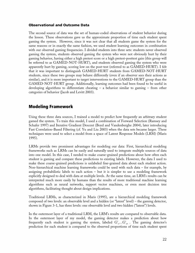
Traditional LRMs, as characterized in Maris (1995), are a hierarchical modeling framework composed of two levels: an observable level and a hidden (or “latent” level) – the gaming detector, shown in Figure 3-1, has three levels: one observable level and two hidden (“latent”) levels. In the outermost layer of a traditional LRM, the LRM’s results are compared to observable data. In the outermost layer of my model, the gaming detector makes a prediction about how frequently each student is gaming the system, labeled G'

0…G'

69 . The gaming detector’s

prediction for each student is compared to the observed proportions of time each student spent

23

gaming the system, G0…G

69 (I will discuss what metrics we used for these comparisons

momentarily). In a traditional LRM, each prediction of an observed quantity is derived by composing a set of predictions on unobservable latent variables – for example, by adding or multiplying the values of the latent variables together. Similarly, in the gaming detector, the model’s prediction of the proportion of time each student spends gaming is composed as follows: First, the model makes a (binary) prediction as to whether each individual student action (denoted P'

m) is an instance of

gaming – a “latent” prediction which cannot be directly validated using the data. From these predictions, G'

0…G'

69 are derived by taking the percentage of actions which are predicted to be

instances of gaming, for each student. In a traditional LRM, there is only one level of latent predictions. In the gaming detector, the prediction about each action P

m is made by means of a linear combination of the characteristics of

each action. Each action is described by a set of parameters; each parameter is a linear, quadratic, or interaction effect on the features of each action distilled from the log files. More concretely, a specific parameter might be a linear effect (a parameter value α

i multiplied by the corresponding

feature value Xi – α

i X

i), a quadratic effect (parameter value α

i multiplied by feature value X

i,

squared – αiX

i

2), or an interaction effect on two parameters (parameter value αi multiplied by

feature value Xi, multiplied by feature value X

j – α

iX

iX

j).

A prediction P

m as to whether action m is an instance of gaming the system is computed as P

m =

α0 X

0 + α

1 X

1 + α

2 X

2 + … + α

n X

n, where α

i is a parameter value and X

i is the data value for the

corresponding feature, for this action, in the log files. Each prediction Pm is then thresholded

using a step function, such that if Pm ≤ 0.5, P'

m = 0, otherwise P'

m = 1. This gives us a set of

classifications P'm for each action within the tutor, which can then be used to create the

predictions of each student’s proportion of gaming, G'0…G'

69 .

24

Figure 3-1: The gaming detector.

Model Selection For the very first detector, trained on just the scatterplot lesson, the set of possible parameters was drawn from linear effects on the 24 features discussed above (parameter*feature), quadratic effects on those 24 features (parameter*feature2), and 23x24 interaction effects between features (parameter* feature

A*feature

B), for a total of 600 possible parameters. As discussed earlier, 2 more

features were added to the data used in later detectors, for a total of 26 features and 702 potential parameters. Some detectors, given at the end of the chapter, omit specific features to investigate specific issues in developing behavior detectors – the omitted features, and the resultant model spaces, will be discussed when those detectors are discussed. The first gaming detector was selected by repeatedly adding the potential parameter that most reduced the mean absolute deviation between our model predictions and the original data, using Iterative Gradient Descent to find the best value for each candidate parameter. Forward Selection continued until no parameter could be found which appreciably reduced the mean absolute deviation. In later model-selection, the algorithm searched a set of paths chosen using a linear correlation-based variant of Fast Correlation-Based Filtering (Yu and Liu 2003). Pseudocode for the algorithm used for model selection is given in Figure 3-2. The algorithm first selected a set of 1-parameter models that fit two qualifications: First, each 1-parameter model of gaming was at least 60% as good as the best possible 1-parameter model. Second, if two parameters had a closer correlation than 0.7, only the better-fitting 1-parameter model was used. Once a set of 1-parameter models had been obtained in this fashion, the algorithm took each model, and repeatedly added the potential parameter that most improved the linear correlation between our model predictions and the original data, using Iterative Gradient Descent (Boyd and Vandenberghe 2004) to find the best value for each candidate parameter. When selecting models for a single tutor lesson, Forward Selection continued until a parameter was selected that worsened the model’s fit under Leave-One-Out-Cross-Validation (LOOCV); when comparing models trained on a single tutor lesson to models trained on multiple tutor lessons, Forward Selection continued until the model had six parameters, in order to control the degree of overfitting due to different sample sizes, and focus on how much overfitting occurred due to training on data from a smaller number of tutor lessons. After a set of full models was obtained, the model with the best A' 4 was selected; A' was averaged across the model’s ability to distinguish GAMED-HURT students from non-gaming students, and the model’s ability to distinguish GAMED-HURT students from GAMED-NOT-HURT students.

4 A' is both the area under the ROC curve, and the probability that if the model has one student from each of the two groups being classified, it will correctly identify which is which. A' is equivalent to W, the Wilcoxon statistic between signal and noise (Hanley and McNeil 1982). It is considered a more robust and atheoretical measure of sensitivity than D' (Donaldson 1993).

25

Two choices in this process are probably worth discussing: the use of Fast Correlation-Based Filtering only at the first step of model selection, and the use of correlation and A' at different stages. I chose to use Fast Correlation-Based Filtering for only the first step of the model search process, after finding that continuing it for a second step made very little difference in the eventual fit of the models selected – this choice sped the model-selection process considerably, with little sacrifice of fit. I chose to use two metrics during the model selection process, after noting that several of the models that resulted from the search process would have excellent – and almost identical – correlations, but that often the model with the best correlation would have substantially lower A' than several other models with only slightly lower correlation. Thus, by considering A' at the end, I could achieve excellent correlation and A' without needing to use A' (which is considerably less useful for iterative gradient descent) during the main model selection process.

Goal: Find model with good correlation to observed data, and good A’

Preset values: σ − How many steps to search multiple paths using FCBF (after

σ steps, the algorithm stops branching) π − What percentage of the best path’s goodness-of-fit is acceptable

as an alternate path during FCBF µ − The maximum acceptable correlation between a potential path’s most

recently added parameter and any alternate parameter with a better goodness-of-fit

ζ − The maximum size for a potential model (-1 if LOOCV is used to set model size)

Data format:

A candidate model is expressed as two arrays: one giving the list of parameters used, and the second giving each parameter’s coefficient.

Prior Calculation Task: Find correlations between different parameters

For each pair of parameters, Compute linear correlation between the pair of parameters, across all actions, and store in an array

Main Training Algorithm: Set the number of parameters currently in model to 0 Set the list of candidate models to empty MODEL-STEP (empty model) For each candidate model (list populated by MODEL-STEP)

Calculate that model’s A’ value (for both GAMED-HURT versus NON-GAMING, and GAMED-HURT versus GAMED-NOT-HURT)

Average the two A’ values together Output the candidate model with the best average A’. Recursive Routine MODEL-STEP: Conduct a step of model search Input: current model

If the current number of parameters is less than σ, Subgoal: Select a set of paths

26

For each parameter not already in the model Use iterative gradient descent to find best model that includes both the

current model and the potential parameter (using linear correlation to the observed data as the goodness of fit metric).

Store the correlation between that model and the data Create an array which marks each parameter as POTENTIAL Repeat

Find the parameter P whose associated candidate model has the highest linear correlation to the observed data

Mark parameter P as SEARCH-FURTHER For all potential parameters Q marked POTENTIAL If the linear correlation between parameter Q and parameter P

is greater than µ, mark parameter Q as NO-SEARCH If the linear correlation between the model with parameter Q and the

observed data, divided by the linear correlation between the model with parameter P and the observed data, is less than π, mark parameter Q as NO-SEARCH

Until no more parameters are marked POTENTIAL For each parameter R marked as SEARCH-FURTHER

Use iterative gradient descent to find best model that includes both the current model and parameter R (using linear correlation to the observed data as the goodness of fit metric).

Recurse MODEL-STEP (new model) Else

Subgoal: Complete exploration down the current path Create variable PREV-GOODNESS; initalize to -1. Create variable L, initialize to -1 Create array BEST-RECENT-MODEL Repeat

For each parameter not already in the model Use iterative gradient descent to find best model that includes both

the current model and the potential parameter (using linear correlation to the observed data as the goodness of fit metric).

Store the correlation between that model and the data Add the potential parameter with the best correlation to the model If ζ = −1 (i.e. we should use cross-validation to determine model size)

Create an blank array A of predictions (of each student’s game freq) For each student S in the data set

Use iterative gradient descent to find best parameter values for the current model, without student S

Put prediction for student S, using new parameter values, into array A

Put the linear correlation between array A and the observed data into variable L

If L > PREV_GOODNESS PREV_GOODNESS = L Put the current model into BEST-RECENT-MODEL

Else Put the current model into BEST-RECENT-MODEL

Until (the model size = ζ OR PREV_GOODNESS > L)

27

Add BEST-RECENT-MODEL to the list of candidate models

Figure 3-2: Pseudocode for the machine learning algorithm used to train the gaming detector

Statistical Techniques for Comparing Models The following methods will be used to conduct statistical analyses in this chapter: This chapter will involve analyses where I compare single models to chance, compare single models to one another, and where I aggregate and/or compare multiple models across multiple lessons. The A' values for single models will be compared to chance using Hanley and McNeil’s (1982) method, and the A' values for two models will be compared to one another using the standard Z-score formula with Hanley and McNeil’s (1982) estimation of the variance of an A' value (Fogarty, Baker, and Hudson 2005). Both of these methods give a Z-score as the result.5 Hanley and McNeil’s method also allows for the calculation of confidence intervals, which will be given when useful. Aggregating and comparing multiple models’ effectiveness to each other, across multiple lessons, is substantially more complex. In these cases, how models’ performance varies across lessons will be of specific interest. Therefore, rather than just aggregating the data from all lessons together, and determining a single measure, I will find a measure of interest (which will be either A' or correlation) for each model in each lesson, and then use meta-analytic techniques (which I will discuss momentarily) to combine data from one model on multiple lessons, and to compare data from different models across multiple lessons. In order to use common meta-analytic techniques, I will convert A' values to Z-scores as discussed above. Correlation values will be converted to Z-scores by converting the correlation to a Fisher Zr and then converting that Fisher Zr to a Z-score (Ferguson 1971) – a comparison of two Z-scores (derived from correlations) can then be made by inverting the sign of one of the Z-scores and averaging the two Z-scores. Once all values are Z-scores, between-lesson comparisons will be made using Stouffer’s method (Rosenthal and Rosnow 1991), and within-lesson comparisons will be made by finding the mean Z-score. The mean Z-score is an overly conservative estimate for most cases, but is computationally simple, and biases to a relatively low degree for genuinely intercorrelated data (Rosenthal and Rubin 1986) (and high intercorrelation is likely, when comparing effective models of gaming in a single data set). After determining a composite Z-score using the appropriate method, a two-tailed p-value is found. Because comparisons made with Stouffer’s method will tend towards a higher Z-score than comparisons that are made with mean Z-score (because of different assumptions), I will note which method is used in each comparison, denoting comparisons made with Stouffer’s method

5 The technique used to convert from A' values to Z-scores (from Hanley and McNeil, 1982) can break down, for very high values of A'; in the few cases where a calculated Z-score is higher than the theoretical maximum possible Z-score, given the sample size, I use the theoretical maximum instead of the calculated value.

28

Zs, comparisons made using mean-Z score Z

m, and comparisons made using both methods Z

ms.

Z-scores derived using only Hanley and McNeil’s method (including Fogarty et al’s variant), with no meta-analytic aggregation or comparison, will simply be denoted Z. Additionally, since Z-scores obtained through Stouffer’s method will be higher than Z-scores obtained through the mean Z-score method, it would be inappropriate to compare a Z-score aggregated with Stouffer’s method to another Z-score aggregated with the mean Z-score method. To avoid this situation, when I conduct comparisons where both types of aggregations need to occur (because there are both between-lesson and within-lesson comparisons to be made), I will always make within-lesson comparisons before any between-lesson comparisons or aggregations. To give a brief example of how I do this, let us take the case where I am comparing a set of models’ training set performance to their test set performance (either A' or correlation), across multiple lessons. The first step will be to compare, for each lesson, the performance of the model trained on that lesson to each of the models for which that lesson is a test set (using the appropriate method for A' or correlation). This gives, for each lesson, a set of Z-scores representing test set-training set comparisons. Then, those Z-scores can be aggregated within-lesson using the mean Z-score method, giving us a single Z-score for each lesson. Next those Z-scores can be aggregated between-lessons using Stouffer’s method, giving a single Z-score representing the probability that models perform better within the training set than the test sets, across all lessons. This approach enables me to conduct both within-lesson and between-lesson comparisons in an appropriate fashion, without inappropriately comparing Z-scores estimated by methods with different assumptions.

A Detector For One Cohort and Lesson My first work towards developing a detector for gaming took place in the context of a lesson on scatterplot generation and interpretation. I eventually gathered data on this lesson from three different student cohorts, using the tutor in three different years (2003, 2004, 2005); my first work towards developing a gaming detector used only the data from 2003, as the work occurred in late 2003, before the other data sets were collected. The 2003 Scatterplot data set contained actions from 70 students, with 20,151 actions in total – approximately 2.6 MB of data. I trained a model, with this data set, treating both GAMED-HURT and GAMED-NOT-HURT students as gaming. I will discuss the actual details of this model (and other models) later in the chapter – focusing in this section on the model’s effectiveness. The ROC curve of the resultant model is shown in Figure 3-3. The resultant model was quite successful at classifying the GAMED-HURT students as gaming (A' = 0.82, 95% Confidence Interval(A') = 0.63-1.00, chance A' =0.50). At the best possible threshold value6, this classifier correctly identifies 88% of the GAMED-HURT students as gaming, while only classifying 15% of the non-gaming students as gaming. Hence, this model can be reliably used to assign interventions to the GAMED-HURT students.

6 ie, the threshold value with the highest ratio between hits and false positives, given a requirement that hits be over 50%

29

However, despite being trained to treat GAMED-NOT-HURT students as gaming, the same model was not significantly better than chance at classifying the GAMED-NOT-HURT students as gaming (A' =0.57, 95% CI(A')=0.35-0.79). Even given the best possible threshold value, the model could not do better than correctly identifying 56% of the GAMED-NOT-HURT students as gaming, while classifying 36% of the non-gaming students as gaming.

Figure 3-3: The model’s ability to distinguish students labeled as GAMED-HURT or GAMED-NOT-HURT, from non-gaming students, at varying levels of sensitivity, in the model trained on the 2003 Scatterplot data.

All predictions used here derived by leave-out-one-cross-validation. Since it is more important to detect GAMED-HURT students than GAMED-NOT-HURT students, we investigated whether extra leverage could be obtained by training a model only on GAMED-HURT students. In practice, however, a cross-validated model trained only on GAMED-HURT students did no better at identifying the GAMED-HURT students (A' =0.77, 95% CI(A') = 0.57-0.97) than the model trained on all students. Thus, in our further research, we will use the model trained on both groups of students to identify GAMED-HURT students.

It is important to note that despite the significant negative correlation between a student’s frequency of gaming the system and his/her post-test score, both in the original data (r= -0.38, F(1,68)=11.82, p<0.01) and in the cross-validated model (r= -0.26, F(1,68)=4.79, p=0.03), the gaming detector did not just classify which students fail to learn. The detector is not better than chance at classifying students with low post-test scores (A' = 0.60, 95% CI(A')=0.38-0.82) or students with low learning (low pre-test and low post-test) (A' =0.56, 95% CI(A')=0.34-0.78). Thus, the gaming detector is not simply identifying all gaming students, nor is it identifying all students with low learning – it is identifying the students who game and have low learning: the GAMED-HURT students.

30

Transfer Across Classes After developing a detector that could effectively distinguish GAMED-HURT students from other students, within the context of a single tutor lesson and student cohort, the next step was to extend this detector to other tutor lessons and student cohorts. In this section, I will talk about my work to extend the detector across student cohorts. Towards extending the detector across student cohorts, I collected data for the same tutor lesson (on scatterplots), in a different year (2004). The 2004 data set contained actions from 107 students, with 30,900 actions in total. The two cohorts (2003 and 2004) were similar at a surface level: both were drawn from students in 8th and 9th grade non-gifted/non special-needs Cognitive Tutor classrooms in the same middle schools in the suburban Pittsburgh area. However, our observations suggested that the two cohorts behaved differently. The 2004 cohort gamed 88% more frequently than the 2003 cohort, t(175)=2.34, p=0.027, but a lower proportion of the gaming students had poor learning, χ2(1, N=64)=6.01, p=0.01. This data did not directly tell us whether gaming was different in kind between the two populations – however, if gaming differed substantially in kind between populations, we thought that two populations as different as these were likely to manifest such differences, and thus these populations provided us with an opportunity to test whether our gaming detector was robust to differences between distinct cohorts of students. The most direct way to evaluate transfer across populations is to see how successfully the best-fit model for each cohort of students fits to the other cohort (shown in Table 3-1). As it turns out, a model trained on either cohort could be transferred as-is to the other cohort, without any re-fitting, and perform significantly better than chance at detecting GAMED-HURT students. A model trained on the 2003 data achieves an A' of 0.76 when tested on the 2004 data, significantly better than chance, Z=2.53, p=0.01. A model trained on the 2004 data achieves an A' of 0.77 when tested on the 2003 data, significantly better than chance, Z=2.65, p=0.01. Additionally, a model trained on one cohort is significantly better than chance – or close – when used to distinguish GAMED-HURT students from GAMED-NOT-HURT students in the other cohort. A model trained on the 2003 data achieves an A' of 0.69 when tested on the 2004 data, marginally significantly better than chance, Z=1.69, p=0.09. A model trained on the 2004 data achieves an A' of 0.75 when tested on the 2003 data, significantly better than chance, Z=2.03, p=0.04. Although the models are better than chance when transferred, there is a marginally significant overall trend towards models being significantly better in the student population within which they were trained than when they were transferred to the other population of students, Z

ms=1.89,

p=0.06. This trend is weaker at the individual comparison level. Only the difference in distinguishing GAMED-HURT students from GAMED-NOT-HURT students, in the 2004 data set, is statistically significant, Z=1.97, p=0.05. The difference in distinguishing GAMED-

7 An alternative explanation is that the two observers were more sensitized to gaming in Study Two than Study One; however, if this were the case, the detector should be more accurate for the Study Two data than the Study One data, which is not the case. Additionally, in the Study Three control condition, the frequency of gaming dropped to almost exactly in between the frequencies from Studies One and Two, implying that the two observers became more sensitized to gaming from Study One to Study Two, and then became less sensitized (or observant) between Study Two and Study Three.

31

HURT students from GAMED-NOT-HURT students, in the 2003 data set, is not quite significant, Z=1.57, p=0.12. The difference in distinguishing GAMED-HURT students from non-gaming students is not significant in either the 2003 or 2004 cohorts, Z=0.59, p=0.55, Z=1.30, p=0.19.

It was also possible to train a model, using the data from both student cohorts, which achieved a good fit to both data sets, shown in Table 3-1. This model was significantly better than chance in all 4 comparisons conducted – the least significant was the unified model’s ability to distinguish GAMED-HURT students from non-gaming students, A'=0.80, Z=3.08, p<0.01. There was not an overall difference between the unified model and the models used in the data sets they were trained on, across the 4 possible comparisons, Z

ms=0.96, p=0.33. There was also not an overall

difference between the unified model and the models used in the data sets they were not trained on, across the 4 possible comparisons, Z

ms=0.94, p=0.35.

Overall, then, although the model does somewhat better in the original cohort where it was trained, models of gaming can effectively be transferred across student cohorts.

Training Cohort

G-H vs no game, 2003 cohort

G-H vs no game, 2004 cohort

G-H vs G-N-H, 2003 cohort

G-H vs G-N-H, 2004 cohort

2003 0.85 0.76 0.96 0.69* 2004 0.77 0.92 0.75 0.94

Both 0.8 0.86 0.85 0.85

Table 3-1. Our model’s ability to transfer between student cohorts. Boldface signifies both that a model is statistically significantly better within training cohort than within transfer cohort, and that the model is significantly better than the model trained on both cohorts. All numbers are A' values. Italics denote a model which is statistically significantly better than chance (p<0.05); asterisks (*) denote marginal significance (p<0.10).

Transfer Across Lessons Transferring Detectors Trained on a Single Lesson – Part One Upon determining that a gaming detector developed for one student cohort could transfer to other student cohorts, within the same lesson, my next step was to investigate whether I could transfer my detector between tutor lessons.

My first step towards extending the detector across tutor lessons was to collect data for a second tutor lesson, covering 3D-geometry. Almost exactly the same set of students used this tutor, and used the scatterplot lesson in 2004: the only differences in sample were because of absence from class. The geometry data set contained actions from 111 students, with 30,696 actions in total. Both the scatterplot and geometry lessons were drawn from the same middle-school mathematics curriculum and were designed using the same general pedagogical principles, although the scatterplot lesson had a greater variety of widgets and a more linear solution path. Our observers did not notice substantial differences between the types of gaming they observed in these two lessons. Overall, there was fairly low overlap between the students observed gaming in each lesson: 15 students were observed gaming in both lessons, 39 students were observed gaming in neither lesson, and 42 students were observed gaming in one lesson but not the other.

32

The most direct way to evaluate transfer across lessons is to see how successfully the best-fit model for each tutor lesson fits to the other tutor lesson (shown in Table 3-2). As it turns out, a model trained on one lesson did not transfer particularly well to the other lesson, without re-fitting. When distinguishing between GAMED-HURT students and non-gaming students, a model trained on the Scatterplot data achieves an A' of 0.55 when tested on the Geometry data, not significantly better than chance, Z=0.75, p=0.55. A model trained on the Geometry data achieves an A' of 0.53 when tested on the Scatterplot data, also not significantly better than chance, Z=0.27, p=0.79. Similarly, a model trained on one lesson is not significantly better than chance when used to distinguish GAMED-HURT students from GAMED-NOT-HURT students in the other cohort. A model trained on the Scatterplot data achieves an A' of 0.41 when tested on the Geometry data, not significantly different than chance, Z=-0.84, p=0.40. A model trained on the Geometry data achieves an A' of 0.63 when tested on the Scatterplot data, not significantly better than chance, Z=1.14, p=0.25. Additionally, there is a significant overall trend towards models being significantly better in the lesson within which they were trained than when they were transferred to the other lesson, Z

ms=4.28, p<0.001. This trend is also present at the individual comparison level, in all four cases.

The difference in distinguishing GAMED-HURT students from non-gaming students, in the Scatterplot lesson (A' of 0.92 versus 0.53), is statistically significant, Z=3.01, p<0.01. The difference in distinguishing GAMED-HURT students from non-gaming students, in the Geometry lesson (A' of 0.80 versus 0.55), is statistically significant, Z=2.88, p<0.01. The difference in distinguishing GAMED-HURT students from GAMED-NOT-HURT students, in the Scatterplot lesson (A' of 0.94 versus 0.41), is statistically significant, Z=4.30, p<0.001. Finally, the difference in distinguishing GAMED-HURT students from GAMED-NOT-HURT students, in the Geometry lesson (A' of 0.90 versus 0.63), is statistically significant, Z=2.13, p=0.03. It was, however, possible to train a model, using both data sets, which achieved a good fit to both data sets, as shown in Table 3-2. This model was significantly better than chance at distinguishing GAMED-HURT students from non-gaming students, both in the Scatterplot lesson, A' = 0.82, Z=3.41, p<0.01, and the Geometry lesson, A' = 0.77, Z=4.62, p<0.001. The model was also marginally significantly better than chance at distinguishing GAMED-HURT students from GAMED-NOT-HURT students in the Scatterplot lesson, A' = 0.70, Z=1.79, p=0.07, and significantly better than chance at distinguishing GAMED-HURT students from GAMED-NOT-HURT students in the Geometry lesson, A' = 0.82, Z=4.10, p<0.001. There was not an overall difference between the unified model and the models used in the lessons they were trained on, across the 4 possible comparisons, Z

ms=1.38, p=0.16, but the unified model

was significantly better than the models used in the lessons they were not trained on, across the 4 possible comparisons, Z

ms=2.69, p=0.01.

Overall, then, a unified model can be developed which transfers across cohorts, but if a model is trained on just one cohort, it does not appear to transfer well to another cohort.

33

Training Lesson

G-H vs no game, SCATTERPLOT

G-H vs no game, GEOMETRY

G-H vs G-N-H, SCATTERPLOT

G-H vs G-N-H, GEOMETRY

SCATTERPLOT 0.92 0.55 0.94 0.63 GEOMETRY 0.53 0.80 0.41 0.90 BOTH 0.82 0.77 0.70* 0.82

Table 3-2. Models trained on the scatterplot lesson, the geometry lesson, and both lessons together. All models trained using only the 2004 students. Boldface denotes the model(s) which are statistically significantly best in a given category. All numbers are A' values. Italics denote a model which is statistically significantly better than chance (p<0.05); asterisks (*) denote marginal significance (p<0.10).

Transferring Detectors Trained on Multiple Lessons

In order to investigate whether a detector trained on multiple lessons would transfer to new lessons, I collected data from two additional lessons in the middle school Cognitive Tutor curriculum, on probability (2004) and percents (2005). This data collection consisted of quantitative field observations giving an estimate for each student’s frequency of gaming, using the method discussed in Chapter 2, pre-tests and post-tests (see Appendix B), and log file records of each student’s actions within the tutor. Additionally, in Study Three, I collected data from a new student cohort using the scatterplots lesson. The probability lesson contained actions from 41 students, with 10,759 actions in total, the percents lesson contained actions from 53 students, with 16,196 actions in all, and the 2005 scatterplot data contained actions from 63 students, with 20,276 actions in all. Hence, I now had data from four different lessons to use, shown in Table 3-3, to investigate whether a detector trained on multiple lessons could be used on another tutor lesson from the same curriculum.

Lesson Number of students Number of actions SCATTERPLOT 268 71,236 PERCENTS 53 16,196 GEOMETRY 111 30,696 PROBABILITY 41 10,759

Table 3-3. Quantity of data available for training, for four different tutor lessons.

Training a Detector on a Single Lesson – Part Two My first step was to train a detector on each of these lessons individually. I then tested this detector for the degree of over-fit to individual lessons, by testing the detector both on the training lesson, and the other three lessons. In this process of training, as well as all of the training I will report in this section, I trained each model to a size of 6 parameters, rather than using Leave-One-Out-Cross-Validation to determine each model’s size, enabling me to focus this investigation on over-fitting due to lesson, rather than over-fitting occurring for other reasons (such as sample size). In all cases, during training, only gamed-hurt students were treated as gaming. The models had an average A' of 0.86 at distinguishing students who gamed in the harmful fashion from students who did not game, in the training lessons, significantly better than chance, Z

s=10.74, p<0.001. The models had an average A' of 0.71 at making the same distinction in the

transfer lessons, also significantly better than chance, Zm

= 2.12, p=0.03. Overall, the models were

34

significantly better at distinguishing harmful gaming in the training lessons than in the transfer lessons, Z

ms =3.63, p<0.001.

The models had an average A' of 0.79 at distinguishing students who gamed in the harmful fashion from students who gamed in the non-harmful fashion, in the training lessons, which was significantly better than chance, Z

s =5.07, p<0.001. The models had an average A' of 0.74 at

making the same distinction in the transfer lessons, also significantly better than chance, Zm

=2.86, p<0.01. Overall, however, the models were not significantly better at distinguishing harmful gaming in the training lessons than in the transfer lessons, Z

ms =0.56, p=0.58.

The models had an average correlation of 0.57 between the observed and predicted frequencies of harmful gaming, in the training lessons, significantly better than chance, Z

s = 12.08, p<0.001.

Within the transfer lesson, the models had an average correlation of 0.22 in the transfer lessons, which was also significantly better than chance, Z

m =2.40, p=0.02. Overall, the models had a

better correlation in the training lessons than in the transfer lessons, Zms

=5.15, p<0.001. Hence, on two of the three metrics of interest, training a detector on each lesson individually produced models that were much better within the lesson they were trained, than in the other lessons. The overall pattern of results from these comparisons is shown in Table 3-4.

Metric Training lesson average Transfer lesson average

A' (GAMED-HURT versus NON-GAMING) 0.86 0.71 A' (GAMED-HURT versus GAMED-NOT-HURT) 0.79 0.74 Correlation 0.57 0.22

Table 3-4. Models trained on just one of the four lessons. Italics denotes when models were, in aggregate, statistically significantly better than chance. Boldface denotes when models were significantly better for training lessons than transfer lessons.

Training a Detector on All Four Lessons The next step was to train a detector on all four of the lessons together, as a benchmark for how good we could expect a multi-lesson detector to be, in order to compare this detector’s effectiveness to detectors trained on a single lesson. The model trained on all four lessons appeared to be equally as effective, across lessons, as the set of four models each trained on a single lesson were for their training lessons. The model trained on all four lessons had an average A' of 0.85 at distinguishing students who gamed in the harmful fashion from students who did not game, compared to an average A' of 0.86 for the models trained on single lessons, not a statistically significant difference, Z

ms = 0.38, p=0.70. The model

trained on all four lessons had an average A' of 0.80 at distinguishing students who gamed in the harmful fashion from students who gamed in the non-harmful fashion, compared to an average A' of 0.79 for the models trained on single lessons, which was not a statistically significant difference, Z

ms = 0.12, p=0.90. Finally, the model trained on all four lessons had an average

correlation of 0.60 between the observed and predicted frequencies of harmful gaming, in the training lessons, compared to an average correlation of 0.57 for the models trained single lessons, not a statistically significant difference, Z

ms = 0.53, p=0.60.

35

Hence, a model can be trained on all four lessons which is on the whole equally as effective as four models trained on individual lessons, testing only on the training sets. The overall pattern of results from these comparisons is shown in Table 3-5. The features of the model trained on all four lessons will be discussed in detail later in the chapter.

Metric Training on one lesson Training on all lessons

A' (GAMED-HURT versus NON-GAMING) 0.86 0.85 A' (GAMED-HURT versus GAMED-NOT-HURT) 0.79 0.80 Correlation 0.57 0.60

Table 3-5. Comparing a model trained on all lessons to models trained on just one of the four lessons, within the training lessons. All models were statistically significantly better than chance, on each metric. No model as significantly better than any other model, on any metric.

Training a Detector on Three of Four Lessons The next question is whether a detector trained on multiple lessons will be more effective when transferred to a new lesson than a detector trained on just one lesson. To investigate this issue, I will train a set of detectors on three of four of the lessons together, and then test each of these detectors on the fourth, left-out, lesson. This will enable me to investigate whether models trained on multiple lessons transfer well to other lessons, from the same curriculum. Since the current gold standard for performance is how well a detector does when trained on a single lesson (on the training-set), I will compare the effectiveness of multiple-lesson trained detectors, on the lesson they were not trained on, to single-lesson trained detectors, on the lesson they were trained on. The models trained on three lessons had an average A' of 0.84 at distinguishing students who gamed in the harmful fashion from students who did not game, in the training lessons, and an average A' of 0.80 at making the same distinction in the transfer lessons. The models trained on one lesson, as discussed earlier, achieved an A' of 0.86 at making this distinction. The difference between the multi-lesson-trained models’ test-set performance was not significantly different than the single-lesson-trained models’ training-set performance, Z

ms = 1.36, p=0.17. In other

words, models trained on three lessons do not perform statistically worse when transferred to a fourth lesson than models trained on a single lesson perform on the lesson they were trained on. The models trained on three lessons had an average A' of 0.78 at distinguishing students who gamed in the harmful fashion from students who gamed in the non-harmful fashion, in the training lessons, and an average A' of 0.80 at making the same distinction in the transfer lessons. At the same, the models trained on single lessons had an A' of 0.79 at making the same distinction, in the lesson they were trained on. The difference between the test-set performance of the models trained on three lessons, and the training-set performance of the models trained on single lessons was not significant, Z

ms = 0.67, p=0.50.

The models trained on 3 lessons had an average correlation of 0.55 between the observed and predicted frequencies of harmful gaming, in the training lessons, and an average correlation of 0.41 in the transfer lessons. By comparison, the models trained on one lesson, as discussed earlier, achieved an average correlation of 0.57 in the training sets. The models trained on one lesson had a marginally significantly better correlation in the training set than the models trained on 3 lessons, in the test sets, Z

ms = 1.74, p=0.08. It is worth remembering, however, that the models

36

trained on one lesson had a correlation of 0.22 in the test sets, significantly worse than the models trained on 3 lessons performed in the test sets, Z

ms = 2.46, p=0.01.

Overall, then, training models on 3 lessons produces a model which is consistently effective on the lessons it is trained on – about as good as a model trained on any one of the lessons alone. At the same time, models trained on 3 detectors show considerably less degradation in transferring to another lesson than models trained on a single detector. In fact, the models trained on 3 lessons were not significantly worse on each model’s transfer lesson than a model trained on one lesson was on its training lessons, in 2 of 3 metrics of interest. The overall pattern of results is shown in Table 3-6.

Metric Training on one lesson (training lessons)

Training on 3 of 4 lessons (transfer lessons)

Training on one lesson (transfer lessons)

A' (GAMED-HURT versus NON-GAMING) 0.86 0.80 0.71 A' (GAMED-HURT versus GAMED-NOT-HURT) 0.79 0.80 0.74 Correlation 0.57 0.41 0.22

Table 3-6. Comparing models trained on all lessons to models trained on just one of the four lessons, within the training lessons. All models were statistically significantly better than chance, on each metric. Grey boxes denote indicate when a model was worse than the best model for that metric (light grey=marginal significance, dark grey = significance).

Transferring Across Lessons – Summary

To sum our results on transferring our gaming detector across lessons: Training the detector on a single lesson results in a detector that performs considerably worse when transferred to a new lesson. However, if we train a detector on multiple lessons, it is effective both within the lessons it was trained for, and on a new lesson that it was not trained for. The results obtained here are from within a single tutor curriculum (cf. Koedinger 2002), and can not be guaranteed to generalize to outside that curriculum. That said, the evidence presented in this section suggests that a gaming detector trained on a small number of lessons (three) from a tutor curriculum will be effective on other lessons from the same curriculum.

Other Investigations of the Gaming Detector A Tradeoff: Detecting Exactly When Students Game The detector I have introduced in this chapter is highly effective at detecting which students game, and how often. However, this detector has a limitation, based on its design, in detecting exactly when students game. This limitation comes in the detector’s use of a student’s prior history. If, for example, a student is assessed as gaming because – among other reasons – they have made a fast error on a problem step after making a considerable number of errors on that step in past problems, it is not entirely clear whether the gaming occurred on the current fast error, or on one or more of the past errors. The detector should be treated as neutral in regards to this question – the most we should infer from the detector is that gaming has occurred on the

37

step of the problem the student just answered, but the gaming may have occurred on this step in a past problem. This distinction is important for two reasons: First, some interventions may be confusing or annoying if they are delivered an entire problem after the gaming actually occurred (for instance, a message saying “You just gamed! Stop gaming!”) Additionally, analyses that depend on determining exactly when students game (which I present in Chapter Four) may be distorted if this issue is not addressed. Therefore, to develop clearer knowledge on exactly when students games, I developed a gaming detector which does not use any data from the student’s actions in prior problems (with the exception of the probability the student knows the current skill, since this metric is unlikely to be vulnerable to the same problem). This involved modifying the following features so that they only involved data from the current problem:

• How many seconds the student spent on each opportunity to practice this skill, within the

current problem. • The total number of times the student has gotten this specific problem step wrong, in the

current problem • The number of times the student asked for help or made errors at this skill, in the current

problem

I also removed the following feature: • What percentage of past problems the student made errors on this step in The resultant detector has 25 features, for a total of 650 potential parameters. When this detector is trained on all 4 tutor lessons, it is moderately less effective than the detector trained using these features. In particular, it is statistically significantly less successful at distinguishing harmful-gaming students from non-gaming students, Z

ms = 2.00, p=0.05, although the magnitude of the

difference between detectors is not very large (A' = 0.82 versus A' = 0.85). It appears to achieve better performance at distinguishing harmful-gaming students from non-harmful-gaming students (A' = 0.82 versus A' = 0.80), Z

ms = 1.02, p=0.31. It also appears to achieve a worse

correlation (r=0.48 versus r=0.60), but this difference is not significant, Zms

= 1.47, p=0.14.

Metric Predictions using

data from past problems

Predictions without data from past problems

A' (GAMED-HURT versus NON-GAMING) 0.85 0.82 A' (GAMED-HURT versus GAMED-NOT-HURT) 0.80 0.82 Correlation 0.60 0.48

Table 3-7. Comparing models that make predictions using data from past problems, to a model that only uses data from the current problem, within the training lessons. All models were statistically significantly better than chance, on each metric. Dark grey boxes denote indicate when a model was statistically significantly worse than the best model for that metric.

The bottom line is that trying to be more confident we know exactly when a student is gaming may slightly lower our ability to be certain we know exactly how much each student is gaming.

38

Hence, the analyses in the remainder of the dissertation use the model which uses data from past problems, unless otherwise noted (one analysis, near the end of Chapter Four, uses the model which is more accurate at detecting exactly when students game, in order to isolate properties of the situations when students game).

Modifying the Detector For Use in a Running Tutor

Another issue in the development of our detector emerged when we used our detector to drive adaptation within our tutor (the tutor’s adaptations are discussed in detail in Chapter Five; in general, the discussion in this section may make more sense after you have read Chapter Five). The detector I have discussed within this chapter is verifiably effective at detecting gaming in student logs. However, the detector had to be modified in subtle ways to be useful for driving adaptation in a running tutor. This is specifically because the tutor that adapts to gaming is different from the tutors the detector was trained on, in that it adapts to gaming. Hence, the detector that we used in the adaptive tutor (in Study Three, Chapter Five) differs from the detector discussed in the rest of this chapter, in that it explicitly accounts for the possibility that some types of interventions will lower the future probability of gaming, on the specific steps of the problem-solving process where the intervention occurred. Developing a principled policy for changing the detector’s assessments after an intervention would require data on student behavior after an intervention; by definition, this sort of data will not be available the first time I introduce an intervention. At the same time, not adapting in some fashion to an intervention raises the possibility of the system acting like a “broken record”: repeatedly intervening on the same step, after the student has stopped gaming. This is a very real possibility, since the detector uses the student’s past actions to help it decide if a student is gaming – past history may be less useful for interpreting the student’s current actions, after an intervention. To address this possibility, I chose a simple “complete forgiveness or no forgiveness” policy for interventions. Within this policy, non-intrusive interventions, such as the animated agent looking unhappy (see Chapter Five) had no effect on the detector’s future assessments. Additionally, if the student gamed during an intervention, future interventions were unchanged. However, if a student received an intrusive intervention, such as a set of supplementary exercises (see Chapter Five), and did not game during that intervention, they received full forgiveness on the problem step that intervention was relevant to: all past history for that step (which is used to make predictions about whether a student is gaming now) was deleted, and the history used in the gaming detector’s predictions for that step began again from a clean slate. Another option, of course, would be to use a detector that never uses past history – however, this decision (as discussed in the previous section) would result in a generally less effective detector. The usefulness of the resulting detector in driving adaptations will be discussed in detail in Chapter Five.

Detector Features In general, the features used in best-fitting models follow a similar pattern, across different training sets. In this section, I will discuss some of the larger cross-model trends and their

39

implications; complete detail on each of the models I discuss in this section is given in Appendix C. One of the first features incorporated into virtually every best-fitting model is a pattern of making a number of errors on the same step, across problems. For example, the best-fitting model for the Study 1 Scatterplot data (“model S1”) has, as its first feature, “ERROR-NOW, MANY-ERRORS-EACH-PROBLEM”, which identifies a student as more likely to be gaming if the student has already made at least one error on the current problem step within this problem, and has also made a large number of errors on this problem step in previous problems. The exact same feature (same parameters, slightly different coefficient) is the first feature in the best-fitting model using all data (“model F”). Even the model trained to not take past problem data (“model NPP”) into account has a feature close to this one as its first feature: “MANY-ERRORS-THIS-PROBLEM”, which identifies a student as more likely to be gaming if the student has made a large number of errors on the current problem step in the current problem. In virtually every model, this type of feature is refined by addressing special cases. These special cases can be expressed either by increasing the probability that many errors on some types of problem steps are evidence of gaming (multiple choice widgets in both model S1 and the Study 1 and 2 Scatterplot model (the model used in Study 3 – “model S1S2”), and asymptotic skills in model S1S2), or by reducing the probability that many errors on some types of problem steps are evidence of gaming (point plotting in models F and NPP, entering numbers in model NPP). The only model that did not contain a special case of this nature was model S1 – in this case, the data set may have been too small to reliably capture potential special cases. Help plays a smaller role than would have been expected from the original definition of gaming. Model S1 did not have internal details of help requests (such as the number of times the student asked for an additional hint, or how long he or she spent on each hint), and had no hint-related features. After building model S1, future data sets collected added data that could be used to distill internal details of help requests, but this did not improve overall model fit, and thus data about internal details of help requests was not used in later models. Nonetheless, help requests do appear in models S1S2, F, and NPP, though never as the first feature selected. Model S1S2’s fourth feature,“HIGH-PERCENTAGE-OF-HELP-REQUESTS-ON-EASILY-LEARNED-SKILLS”, identifies a student as more likely to be gaming if he or she frequently requests help on the skills which students, in general, learn on their first couple opportunities to practice the skill. Model F’s second feature, “ASKING-FOR-HELP-ON-WELL-KNOWN-STEPS”, identifies a student as more likely to be gaming (or to have gamed in the past) if the student asks for help on skills that he or she has a high probability of knowing. In effect, this feature suggests that the student may have in the past obtained correct answers through lucky guesses, or through problem-specific strategies. Model NPP’s second feature, “CLUSTER-OF-HELP-REQUESTS-WHILE-ENTERING-STRINGS”, identifies a student as more likely to be gaming if the student asks for help several times in a short period of time on skills that require entering a string. Interestingly, models F and NPP refine the link between gaming and help use with later features. Model F’s fifth feature,“CLUSTERS-OF-HELP-REQUESTS-ARE-NOT-GAMING”,

identifies that a cluster of help requests in quick succession is not gaming. This feature serves to refine Feature “ASKING-FOR-HELP-ON-WELL-KNOWN-STEPS”, reducing the intensity of “ASKING-FOR-HELP-ON-WELL-KNOWN-STEPS”’s effects when a student who has done well on early problems finds some feature of a later problem enigmatic across several steps.

40

Model NPP’s sixth feature, “ASKING-FOR-LOTS-OF-HELP-IS-NOT-GAMING”, is similar, suggesting that a high proportion of help requests on a single skill within one problem is unlikely to be gaming. Another type of feature that occurs in several models is a feature that specifically identifies well-known skills or slow actions as unlikely to signify gaming. In model S1, “SLIPS-ARE-NOT-GAMING”

identifies that if a student has a high probability of knowing a skill, the student is less

likely to be gaming, even if he or she has made many errors recently. In model F, “SLOW-CORRECT-ANSWERS-ARE-NOT-GAMING” suggests that slow correct answers are not gaming. In model NPP, “SLOW-ACTION-AFTER-MANY-ERRORS-IS-NOT-GAMING” indicates that if a student makes a slow action after making a number of errors, they are probably not gaming. Overall, then, the models largely included the same types of features, capturing similar types of behavior, but with differences at the margins – and predominantly in the later features selected (which were more likely to capture special cases). Interestingly, the model that appeared to have the greatest appearance of overfitting was model S1S2, with 5 of 6 features appearing to deal with special cases – one possibility is that this model, trained on a considerable amount of data but from only the Scatterplot lesson, is overfit to the single lesson it was trained on (instead of the individual students it was trained on) Each of the models discussed in this section is discussed in complete detail, feature by feature, in Appendix C.

Contributions My work towards developing a generalizable detector of gaming has produced three primary contributions. The first contribution, immediately relevant to the topic of this thesis, is the fact that we have developed a gaming detector that verifiably works on a number of tutor lessons, and which can be used to detect gaming within new tutor lessons without large degradations in performance. This work establishes that is possible to develop a behavior detector that can transfer effectively between fairly different lessons within-curriculum. The results presented here also suggest that it is beneficial to train on multiple lessons, to obtain a detector which can be generalized to lessons beyond the original training lessons. The second contribution is in the adaptation of a psychometric framework, Latent Response Models, for use in machine-learned behavior detection. LRMs have a number of advantages for behavior detection, being able to naturally take advantage of multiple sources of data at different grain-sizes. My work in adapting LRMs to this task involved developing a new type of three-level LRM, and inventing a new algorithm – based on forward selection, iterative gradient descent, and Fast Correlation-Based Filtering, to search the space of potential LRMs. The techniques I developed for learning LRMs have proved useful not just in developing a detector of gaming, but have also proved useful for mining information about other types of behavior in Cognitive Tutor log files (see Chapter 4 for a fuller discussion of the use of LRMs for data mining). I believe that LRMs will be useful in a considerable range of behavior detection and data mining problems – essentially, whenever there is fine-grained data from log files that can be combined with aggregate, user-by-user data.

41

A third contribution of this portion of my thesis is towards understanding what sorts of data is useful in developing detectors to understand student behavior. It is not surprising that both log file data, and direct observations of the behavior of interest are useful. It is interesting, however, that it is still useful to have direct observations, even when those direct observations cannot be directly linked to specific actions in the log files. It is also interesting that we needed data from outcome measures in order to interpret our detector’s results. Without measures of each student’s learning, it would have appeared that our detectors were only succeeding in detecting some gamers. With that data, it becomes clear that our detectors can successfully distinguish two types of gaming at the same time that they can distinguish gaming students from non-gaming students.

42

Chapter Four Understanding Why Students Game

In this chapter, I discuss my work towards developing a profile of why students game. In order to do this, I will consider evidence from two attitudinal surveys, student statements as they worked with the tutor, and evidence from our detector as to what behaviors are associated with gaming. Along the way, I will present disconfirmatory evidence for some of the most popular explanations for why students game.

Study One Our first study on gaming demonstrated that gaming was associated with poor learning outcomes. It also provided some evidence on which students game, evidence that I used in order to generate hypotheses as to why students choose to game. I then investigated these hypotheses in detail in Studies Two and Three. In this section, I will discuss the evidence from Study One, relevant to this issue. Details on this study (sample size, population, and so on) are given in Chapter Two, as is evidence on the effects of gaming and other behaviors on learning; in this section, I will present evidence from Study One on what characterizes the students who game. The first distinguishing characteristic about gaming students, from Study One, is their degree of prior knowledge about the subject matter in the tutor lesson. Not all students with low pre-test scores gamed the system, but all of the students who gamed frequently (more than the median amount of gaming, among gaming students) had low pre-test scores. More generally, there was a significant correlation between how frequently a student gamed the system and their pre-test score, F(1,68)=5.31,p=0.02, r= -0.27. There was an apparent marginal correlation between frequency of gaming and performance on the test of general academic achievement, F(1,61)=2.77, p=0.10, r=-0.21, but this relationship ceased to be near significance when we controlled for each student’s performance on the pre-test, F(1,60)=0.22, p=0.64. There was also not a significant relationship between what teacher the student had and the frequency of gaming the system, F(3,66)=0.99,p=0.41. There was also not a significant relationship between gaming the system and off-task behavior, F(1,68)=0.33, p=0.57. The 8 high-gaming students engaged in off-task behaviors (such as talking to other students or surfing the web) with about the same frequency (15%) as the never-gaming students did (14%). We interpreted the lack of connection between gaming and off-task behavior as evidence that gaming did not occur due to lack of interest in material – if students gamed solely out of lack of interest, we might expect them to engage more frequently in completely off-task behavior as well. However, there was a fairly strong relationship between a student’s frequency of gaming the system and that student’s frequency of talking to the teacher or another student about the subject matter, F(1,68)=10.52,p<0.01, r=0.37. This relationship remained after controlling for prior knowledge and general academic achievement, F(1,59) = 8.90, p<0.01, partial correlation = 0.36. One possible explanation for this finding is that gamers, when they talk about the subject matter, were attempting to obtain the answers to problems without having to try to figure out the answer

43

(a strategy similar to gaming), a behavior observed in traditional classrooms (Arbreton, 1998). Interestingly, this type of help-seeking behavior has been found to be associated with having performance goals rather than learning goals (Arbreton, 1998). However, another possible explanation for the relationship between gaming and talking to the teacher is that when a teacher observes a student gaming, he/she tries to help the student with the material. Finally, there was not a statistically significant relationship between gender and the frequency of gaming the system, F(1,68)=1.02, p=0.31.

Prior Knowledge (Pre-Test)

General Academic Achievement

Other Off-Task Behavior

Talking On-Task

Gender

Gaming the System - 0.27 - 0.21 0.07 0.37 0.12

Table 4-1. The correlations between gaming the system and other measures, in Study One. Statistically significant relationships are in boldface, marginally significant relationships are in italics Evidence from the Gaming Detector One advantage of developing a detector for gaming is that it extended our evidence about student gaming. Before developing the detector, we knew which students gamed the system, and how often; our detector gave us additional evidence (though not completely conclusive evidence) on when students gamed the system. The detector was able to do this, because it made predictions about whether each action was a gaming incident en-route to predicting each student’s frequency of gaming. In this section, I will discuss what we were able to learn about gaming, from analyzing the first version of our gaming detector (trained on just the Study One data from the scatterplot lesson). Our detector shed light on gaming in several fashions. The first was in how gaming actions are distributed across a student’s actions. 49% of the detector’s gaming predictions occurred in clusters where at least 2 of the nearest 4 actions were also instances of gaming. To determine the chance frequency of such clusters, I ran a Monte Carlo simulation where each student’s instances of predicted gaming were randomly distributed across that student’s 71 to 478 actions. In this simulation, only 5% (SD=1%) of gaming predictions occurred in such clusters. Hence, our detector predicted that substantially more gaming actions occur in clusters than one could expect from chance. The second was in dividing gaming into two distinct behaviors, harmful gaming and non-harmful gaming. These two types of gaming appeared identical to the observers in Study One (and in each study afterwards), but in training the gaming detector, I found that students in these categories were behaviorally distinct (see Chapter Three). Additionally, the two types of gaming were associated with substantially different learning outcomes. Students who engaged in harmful gaming showed almost no learning, while students who engaged in non-harmful gaming scored well on the post-test (in some cases, apparently because they already knew the material at pre-test). In the rest of this section, I will refer to students who gamed in the harmful fashion as GAMED-HURT students, and students who gamed in the non-harmful fashion as GAMED-NOT-HURT students. Beyond simply distinguishing harmful gaming from non-harmful gaming, the gaming detector suggested that there was at least one substantial difference between GAMED-HURT and

44

GAMED-NOT-HURT students: when they choose to game. This difference manifested itself when I compared the model’s predicted frequency of gaming on “difficult skills”, which the tutor estimated the student had under a 20% chance of knowing (20% was the tutor’s estimated probability that a student knew a skill upon starting the lesson), to the frequency of gaming on “easy skills”, which the tutor estimated the student had over a 90% chance of knowing. The gaming detector predicted that students in the GAMED-HURT group gamed significantly more on difficult skills (12%) than easy skills (2%), t(7)=2.99, p=0.02 for a two-tailed paired t-test. By contrast, the gaming detector predicted that students in the GAMED-NOT-HURT group did not game a significantly different amount of the time on difficult skills (2%) than on easy skills (4%), t(8)=1.69, p=0.13. This pattern of results (shown in Table 4-2) suggested that the difference between GAMED-HURT and GAMED-NOT-HURT students may be that GAMED-HURT students chose to game exactly when it will hurt them most (which in turn may explain why GAMED-HURT students learned less!).

Students Hardest skills (under 20% probability that the student knows)

Easiest skills (over 90% probability that the student knows)

Significance of difference

GAMED-HURT 12% 2% p=0.02 GAMED-NOT-HURT 2% 4% p=0.13

Table 4-2. How frequently students game on steps they have different levels of understanding of.

The evidence that GAMED-HURT students game overwhelmingly on the hardest skills suggests another hypothesis for why these students may be gaming. The choice to withdraw effort exactly where the consequences will be highest seems similar to the set of behaviors termed “learned helplessness”, where students actively avoid effort on difficult challenges in order to justify the failure that they expect will occur regardless of how hard they work (Dweck 2000). In this case, perhaps students who game attribute their early difficulties in a tutor lesson (which stem from low prior-knowledege) to a more global lack of aptitude, and avoid the difficult challenges implicit in learning the tutor material.

Study Two After analyzing data from our first study, and from the gaming detector, we conducted a second study to determine why students game. As discussed in Chapter Two, this study also replicated our earlier finding that gaming was negatively associated with learning. In this study, we used an attitudinal questionnaire to assess student attitudes, and then determined which attitudes were most associated with harmful gaming (as assessed by the gaming detector). We also collected further data on the relationship between different types of student behavior.

Hypotheses In Study Two, we investigated four broad hypotheses about why students game, shown in Table 4-3.

45

Students game because they... Relevant literature

have performance goals instead of learning goals (Elliott and Dweck, 1988) have learned helplessness, stemming from educational anxiety (Dweck, 1975; Dweck, 2000) dislike the tutor/computer (Frantom, Green, and Hoffmann 2002) are prone to deception in educational settings (cf. Sarason 1978)

Table 4-3. Study Two hypotheses on why students game.

The performance goals hypothesis stemmed from evidence in Study One, showing that students who gamed the system also talked more about the subject matter with the teachers and other students. We hypothesized that students who talk more about the subject matter may actually be trying to get others to give them the answer, a behavior found to be correlated to performance goals (Arbreton 1998). For this reason, both our research group (e.g. Baker, Corbett, Koedinger, and Wagner 2004) and other researchers (Martinez-Mirón, du Boulay, and Luckin 2004) hypothesized before this study that students game because of performance goals. The anxiety hypothesis came from evidence that students game on the steps they know least well, based on potential links between gaming and learned helplessness (see Chapter Three). The teachers we work with also hypothesized that gaming would be connected with anxiety, based on their classroom experiences and intuition.

Methods Study Two took place within 6 middle-school classes at 2 schools in the Pittsburgh suburbs. Student ages ranged from approximately 12 to 14. As discussed in Chapter One, the classrooms studied were taking part in the development of a new 3-year Cognitive Tutor curriculum for middle school mathematics. 102 students were present for all phases of the study (other students, absent during one or more days of the study, were excluded from analysis). I studied these classrooms during the course of the same Cognitive Tutor lesson on scatterplot generation and interpretation used in Study One. The day before students used the tutoring software, they viewed a PowerPoint presentation giving conceptual instruction (shown in Chapter One). Within this study, I combined the following sources of data: a questionnaire on student motivations and beliefs, logs of each student’s actions within the tutor (used with the gaming detector, to make predictions of how often each student gamed), and pre-test/post-test data. Quantitative field observations were also obtained, as in Study One, as both a measure of student gaming and in order to improve the gaming detector’s accuracy. These observations had high inter-rater reliability (see Chapter Two). The questionnaire consisted of a set of self-report questions given along with the pre-test, in order to assess students’ motivations and beliefs. The questionnaire items were drawn from existing motivational inventories or from items used across many prior studies with this age group, and were adapted minimally (for instance, the words “the computer tutor” was regularly substituted for “in class”, and questions were changed from first-person to second-person for consistency). All items were pre-tested for comprehensibility with a student from the relevant age group before the study. The questionnaire included items to assess:

46

• Whether the student was oriented towards performance or learning (2 items, 4 choices) (e.g. Mueller and Dweck 1998) “We are considering adding a new feature to the computer tutors, to give you more control over the problems the tutor gives you. If you had your choice, what kind of problems would you like best?

A) Problems that aren’t too hard, so I don’t get many wrong. B) Problems that are pretty easy, so I’ll do well. C) Problems that I’m pretty good at, so I can show that I’m smart D) Problems that I’ll learn a lot from, even if I won’t look so smart.”

“Some classes that use computer tutors also have extra-credit projects. If you had your choice, what kind of extra projects would you most like to do?

A) An extra-credit project that is easy, so I can get a better grade. B) An extra-credit project where I could learn about things that interested me. C) An extra-credit project in an area I’m pretty good at, so I can show my

teacher what I know. D) An extra-credit project that isn’t very difficult, so I don’t have to work too

hard.”

• The student’s level of anxiety about using the tutor (2 items, scale 1-6) (e.g. Harnisch, Hill, and Fyans 1980) “When you start a new problem in the tutor, do you feel afraid that you will do poorly?” “When you are working problems in the tutor, do you feel that other students understand the tutor better than you?”

• The student’s level of anxiety about using computers (1 item, scale 1-6) (e.g. Harnisch, Hill, and Fyans 1980) “When you use computers in general, do you feel afraid that you will do something wrong?”

• How much the student liked using the tutor (2 items, scale 1-6) (e.g. Mueller and Dweck, 1998) “How much fun were the math problems in the last computer tutor lesson you used?” “How much do you like using the computer tutor to work through math problems?”

• The student’s attitude towards computers (1 item, scale 1-6) (e.g. Frantom, Green, and Hoffman 2002) “How much do you like using computers, in general?”

• If the student was lying or answering carelessly on the questionnaire. (1 item, 2 choices) (e.g. Sarason 1978) “Is the following statement true about YOU? ‘I never worry what other people think of me’. TRUE/FALSE”

In analyzing the relationship between gaming and student attitudes, I will use the gaming detector’s assessments as a measure of each student’s incidence of harmful and non-harmful gaming rather than direct observations of gaming, for two reasons: First, because the direct observations do not distinguish between harmful gaming and non-harmful gaming whereas the detector successfully makes this distinction – and the two types of gaming may arise from

47

different motivations. Second, because the gaming detector’s assessments are more precise than the classroom observations – 2-3 researchers can only obtain a small number of observations of each student’s behavior, but the gaming detector can make a prediction about every single student action. Finally, the same pre-tests and post-tests used in Study One were given in order to measure student learning. See Appendix B for a full discussion of these tests. Results Within Study Two, two types of questionnaire items were found to be significantly correlated to the frequency of gaming, as shown in Table 4-4: a student’s attitude towards computers, and a student’s attitude towards the tutor. Students who gamed in the harmful fashion (as assessed by the detector) liked computers significantly less than the other students, F(1,100)=3.94, p=0.05, r = -0.19, and liked the tutor significantly less than the other students, F(1,100)= 4.37, p=0.04, r= -0.20. These two metrics were related to each other: how much a student liked computers was also significantly positively correlated to how much a student liked the tutor, F(1,100)= 11.55, p<0.01, r= 0.32. Gaming in the non-harmful fashion was not correlated to disliking computers, F(1,100) = 1.71, p=0.19, or disliking the tutor, F(1,100)=0.40, p=0.53.

By contrast, our original hypotheses for why students might game did not appear to be upheld by the results of this study. Neither type of gaming was correlated to having performance goals (defined as answering in a performance-oriented fashion on both questionnaire items), F(1,100)=0.78, p=0.38, F(1,100)=0.0,p=0.99. Furthermore, a student’s reported level of anxiety about using the tutor was not associated with choosing to game the system, in either fashion, F(1,100) = 0.17, p=0.68, F(1,100) = 1.64, p= 0.20 and a student’s reported level of anxiety about using computers was not associated with choosing to game the system, in either fashion, F(1,100)=0.04, p=0.84, F(1,100) = 0.58, p=0.45. Finally, a student’s decision to lie or answer carelessly on the questionnaire was not associated with choosing to game the system, in either fashion, F(1,98)=0.37, p=0.55, F(1,98)= 0.95, p=0.33.

Performance Goals

Anxiety about Using Computers

Anxiety about Using

the Tutor

Lying/ Answering Carelessly

Liking Computers

Liking the

Tutor Gaming the System (Harmful fashion)

0.00 -0.02 -0.04 0.06 - 0.19 - 0.20

Post-Test 0.15 -0.02 0.04 0.03 -0.32 0.10

Table 4-4. Correlations between gaming the system, the post-test (controlling for pre-test), and items on the Study Two motivational/attitudinal questionnaire. Statistically significant relationships (p<0.05) are in italics.

One interesting side-result was that while harmful gaming was correlated with poorer learning (see Chapter Two), and harmful gaming was correlated with negative computer attitudes, negative attitudes towards computers were associated with poorer learning, even when we controlled for the relationship between harmful gaming and learning, F(1,96)= 8.48, p<0.01. The link between harmful gaming and post-test also remained marginally significant when computer attitudes (along with pre-test) were partialed out, F(1,96)=3.54, p=0.06. By contrast, a student’s attitude towards the tutor was not significantly correlated to his/her post-test score, F(1,97) = 0.99, p=0.32, controlling for pre-test.

48

At this point, our original hypothesis (that gaming stems from performance goals) appeared to be disconfirmed. On the other hand, we now knew that students who game dislike computers and the tutor. This raised new questions: Why do students who dislike computers and the tutor game? What aspects of disliking computers and the tutor are associated with gaming? One possibility we considered is that a student who has a negative attitude towards computers and the tutor may believe that a computer cannot really give educationally helpful hints and feedback – and thus, when the student encounters material she does not understand, she may view gaming as the only option. Alternatively, a student may believe that the computer doesn’t care how much he learns, and decide that if the computer doesn’t care, he doesn’t either. A third possibility we considered is that a student may game as a means of refusing to work with a computer she dislikes, without attracting the teacher’s attention. All three of these possibilities are consistent with the results of Study Two; in Study Three, we will probe the link between disliking computers and the tutor and the choice to game the system more deeply. Relationship Between Gaming and Talking to the Teacher: Failure to Replicate Earlier Result One of our more suggestive findings from Study One was that gaming was correlated to talking to the teacher or other students on-task were correlated. However, this finding was not replicated in Study Two. There was not a significant relationship between observed gaming and talking on-task, t(103)= 1.07, r = -0.10, p = 0.29 for a two-tailed t-test, nor between detected gaming (combined across types) and talking on-task, t(92)= 1.06, r = 0.11, p=0.29 for a two-tailed t-test. In Study Two, we collected observations that let us split talking on-task into two groups of behavior: requesting answers, and all other types of talking on-task (including discussing the subject matter and discussing how to find the answer). Neither of the two types of gaming were significantly correlated to either of the two types of talking on-task (four comparisons, none with p lower than 0.14). Evidence on Performance Goals At the beginning of Study Two, a primary hypothesis was that performance goals would be associated with a student’s choice to game the system. However, as discussed earlier in this chapter, this hypothesis was not upheld: we did not find a connection between whether a student had performance goals and whether that student gamed the system. Instead, performance goals appeared to be connected to a different pattern of behavior: working slowly, and making few errors. Students with performance goals (defined as answering in a performance goal-oriented fashion on both questionnaire items) answered on tutor problem steps more slowly than the other students, F(1,29276)=39.75, p<0.001, controlling for the student’s pre-test score and the student’s knowledge of the current tutor step8. Overall, the median response time of students with performance goals was around half a second slower than that of the other students (4.4s .vs. 4.9s). Students with performance goals also made fewer errors per problem step than other students, F(1,15854)= 3.51, p=0.06, controlling for the student’s pre-test score. Despite having a

8 It is necessary to control for the student’s knowledge of the current step for this analysis, since students who make more errors would be expected to have more actions on skills they know poorly – and actions on skills known poorly might be faster or slower in general than well-known skills.

49

different pattern of behavior, students with performance goals completed the same number of problem-steps as other students, because slower actions were offset by making fewer errors, t(100)=0.17, p=0.86 (an average of 159 steps were completed by students with performance goals, compared to 155 steps for other students). Similarly, students with performance goals did not perform significantly better or worse on the post-test (controlling for pre-test) than other students – if anything, the trend was in the direction of better learning among students with performance goals, F(1,97)=2.13, p=0.15. One possible explanation for why students with performance goals worked slowly and avoided errors rather than gaming is that these students may have focused on performance at a different grain-size than we had expected. We had hypothesized that students with performance goals would more specifically have the goal of performing well over the course of days and weeks, by completing more problems than other students – a goal documented in past ethnographic research within Cognitive Tutor classes (Schofield 1995). We hypothesized that, in order to realize that goal, students would game the system. However, a student with another type of performance goal might focus on maintaining positive performance minute-by-minute. Such a student would set a goal of continually succeeding at the tutor, avoiding errors and attempting to keep their skill bars continually rising. These students could be expected to respond more slowly than other students, in order to avoid making errors – which is the pattern of behavior we observed. On the whole, within Study Two, students with performance goals used the tutor differently than other students, but by working slowly and avoiding errors rather than by gaming the system. It is not yet entirely clear why students with performance goals chose to use the tutor in this fashion – one possible explanation is that these students focused on performance at a different grain-size than expected. In general, it appears that performance goals are not harming student learning, since students with performance goals learned the same amount as the other students. Therefore, recognizing differences in student goals and trying to facilitate a student in his/her goal preferences (cf. Martínez-Mirón, duBoulay, and Luckin 2004) may lead to better educational results than attempting to make all students adopt learning goals.

Study Three After analyzing data from Studies One and Two, we conducted a third study to hone in on why students game. In this study we focused on investigating, in greater detail, the link between gaming and disliking computers and the tutor. To investigate this issue, we used a design similar to the design in Study Two, giving students an attitudinal questionnaire to assess their attitudes, and then determining which attitudes were most associated with harmful gaming (as assessed by the gaming detector).

Hypotheses In Study Three, we investigated a set of 6 student characteristics that we thought might inform our understanding of why students choose to game the system, shown in Table 4-6.

50

Label Student Characteristic

A The student believes that computers in general, and the tutor in specific, are not very useful. B The student believes that computers don’t/can’t really care how much he/she learns. C The student has a tendency towards passive-aggressiveness (Parker and Hadzi-Pavlovic 2001) D The student believes that computers/the tutor reduce his/her sense of being in control E The student is not educationally self-driven F The student dislikes math

Table 4-6. Characteristics studied, in relation to harmful gaming, in Study Three.

Characteristics A through D were drawn from the literature, as potential hypotheses motivating the link between disliking computers/the tutor and gaming the system, shown in Table 4-6. Characteristics E and F represent more indirect potential links between disliking computers/the tutor and gaming the system; we hypothesized that, if a student were not self-driven or disliked math, he or she might dislike a tutoring system that made him or her persist in completing math problems. Characteristic E appears to be consistent with results published by Arroyo and Woolf in 2005 (at the same time as Study Two was published, three months after Study Three had finished running), indicating that making more errors and spending less time reading help, a pattern of behavior which likely includes gaming, is correlated to having the goal of completing work with an intelligent tutor lesson as quickly as possible. The items used to assess these attitudes and characteristics are given in Table 4-7. All items were drawn from existing attitudinal inventories or had been validated in prior studies. Some items were adapted minimally in order to shift their domain to the context of a tutoring system. Item

Associated Characteristic

Item Drawn From

“Most things that a computer can be used for, I can do just as well myself.”

A Selwyn, 1997

“The tutor’s help system is effective in helping me complete problems.”

A Lewis, 1995

“I feel that the tutor, in its own unique way, is genuinely concerned about my learning.”

B Bickmore and Picard, 2004

“The tutor treats people as individuals” B Cupach and Spitzberg, 1983 “The tutor ignores my feelings” B Cupach and Spitzberg, 1983 “At times I tend to work slowly or do a bad job on tasks I don’t want to do”

C Parker and Hadzi-Pavlovic, 2001

“I tend to try to get out of things by making up excuses”

C Parker and Hadzi-Pavlovic, 2001

“I often forget things that I would prefer not to do” C Parker and Hadzi-Pavlovic, 2001 “Using the tutor gives me greater control over my work”

D Dillon et al, 1998

“I am in complete control when I use a computer” D Selwyn, 1997 “I study by myself without anyone forcing me to study.”

E Knezek and Christensen, 1995

“I try to finish whatever I begin” E Knezek and Christensen, 1995 “I enjoy working on a difficult math problem” F Knezek and Christensen, 1995 “Math is boring” F Knezek and Christensen, 1995

Table 4-7. Items used within the Study Three questionnaire.

51

Methods Study Three took place within 5 middle-school classes at 2 schools in the Pittsburgh suburbs. Student ages ranged from approximately 12 to 14. As discussed in Chapter One, all students were participating in a year-long Cognitive Tutor class teaching middle school mathematics, and the study was conducted in the spring semester, after students had used the Cognitive Tutor for long enough that they presumably had learned how to game if they wanted to, and would not be discovering gaming for the first time during the study. 108 students participated in this study; 95 students completed at least part of the questionnaire and used the Cognitive Tutor during at least one class session during the half of the study relevant to this chapter (and will be used in analysis where appropriate). Study Three had two parts. In this chapter, we will discuss the first part of Study Three – the second part of Study Three, concerning a pair of interventions to respond to gaming, will be discussed in detail in Chapter Five. In the first part of Study Three, students used an unmodified Cognitive Tutor lesson drawn from their standard curriculum. Half of the students (53% of students present for the entire study) worked with a lesson on converting between percents and other mathematical representations; the other students worked with a lesson on creating and interpreting scatterplots of data. All students used the tutor for 80 minutes of class time (spread across either 2 or 3 class days, in accordance with differences in school period length between school districts). Before and after using the tutor, students completed a pre-test and post-test in order to measure their learning. Along with the pre-test, students completed a questionnaire on their attitudes and characteristics, made up of the items in Table 4-7. All questionnaire items were given as Likert scales, from 1 to 6. A student’s score for each of the characteristics in Table 4-6 is the average of their responses on each of the relevant items in Table 4-7, with scores reversed as necessary for inter-scale consistency. In Study Three, as in Study Two, we use the machine-learned detector of harmful gaming (described in Chapter Three) to indicate what proportion of the time each student engaged in a specific type of gaming found to be associated with poorer learning. I use the detector rather than human observations for the same reason I used the detector in Study Two – greater precision, and the ability to distinguish between harmful gaming and non-harmful gaming. In the analyses presented here, I use a detector trained on data from the Scatterplot lesson in Studies One and Two. Results The characteristic most correlated to harmful gaming (as assessed by the gaming detector) in Study Three was a lack of educational self-drive (characteristic E), F(1,92)=6.10, p=0.02, r = 0.25. To make the relationship between harmful gaming and lack of educational self-drive more concrete, if we compare the least self-driven quartile of students to the most self-driven quartile of students, we find that the least self-driven quartile engaged in harmful gaming 68% more frequently than the most self-driven quartile (6.2% of the time versus 3.7% of the time), a marginally significant but fairly large difference, t(44)=1.88, p=0.07, effect size = 0.71 SD. This result is compatible with the recent findings by Arroyo and Woolf (2005), where a student’s reported desire to complete their work with the tutor as quickly as possible with minimal effort (measured in their study by the item “I just wanted to get the session over with, so I went as fast as possible without paying much attention”) (a goal likely related to lack of educational self-drive)

52

was found to be correlated to making more errors and reading help more quickly (behaviors connected to gaming). Another characteristic significantly correlated to harmful gaming in Study Three was disliking math (characteristic F), F(1,92)=4.20, p=0.04, r= 0.21. To make the relationship between harmful gaming and disliking math more concrete, the quartile of students that disliked math the most engaged in harmful gaming 63% more frequently than the quartile of students who liked math the best (4.9% of the time versus 3.0% of the time), although this difference fell short of statistical significance, t(44)=1.54, p=0.13, effect size = 0.60 SD. No other characteristic was significantly correlated to harmful gaming, as shown in Table 4-8. However, although the belief that computers and the tutor are not useful (characteristic A) was not significantly correlated to harmful gaming, F(1,93)=2.51,p=0.12, r= 0.16, the trend was strong enough to suggest that this hypothesis may be worth investigating in greater detail in future studies. None of the other three characteristics (B,C, and D) were significantly correlated with harmful gaming, F(1,90)=1.55, p=0.22, r= 0.13; F(1,92)=0.76, p= 0.36, r=0.10; F(1,93)=0.17, p=0.68, r= 0.04.

Belief that Computers/ the Tutor are

not useful (A)

Belief that Computers/ the Tutor

are uncaring (B)

Tendency towards passive-

aggressiveness (C)

Belief that Computers/ the Tutor

reduce control (D)

The student is not self-driven

(E)

Disliking math (F)

Gaming the System (Harmful fashion)

0.16 0.13 0.10 0.04 0.25 0.21

Table 4-8. Correlations between gaming the system and characteristics assessed in this study. Statistically significant relationships (p<0.05) are in italics.

Evidence from the Gaming Detector – Studies Two and Three: What Steps Do Students Game On? After Study One, a gaming detector trained with just the data from Study One (a single lesson, on scatterplots) provided evidence suggesting that students gamed in the harmful fashion far more on the hardest steps than the easiest steps (where hardest is defined as a lower than 20% probability that the student knows the skill at the time, and easiest is defined as a higher than 90% probability that the student knows the skill at the time). In this section, I replicate this analysis with an improved detector trained on four tutor lessons, including the data from Studies Two and Three presented here (discussed in detail in Chapter Three). For this analysis, I use the detector trained to make the most accurate predictions about exactly when each student is gaming (model “NPP” in Appendix C), rather than a detector trained to make the most accurate overall predictions about which students game and how often, since the goal of the analysis presented here is to determine when students game. Using this detector, we find that students game harmfully over twice as often on the hardest steps as on the easiest steps (34% of the time versus 15% of the time9), a significant difference,

9 This detector, as noted in Chapter 3, has a tendency to overestimate how often all students game, although it still accurately identifies gaming students and correlates well to actual gaming.

53

t(293)=13.92, p<0.001, for a paired t-test. Overall, there is a statistically significant linear relationship between the difficulty of a step, and the frequency of gaming, F(1, 3748)= 224.5, p<0.001, r= - 0.24, shown in Figure 4-1. This result is especially interesting, in light of the fact that this detector does not include the probability the student knows the skill in any of its seven features (not by design – it just wasn’t selected for during model selection); hence, the pattern observed is an emergent property of the data, not just a consequence of a specific feature in the model.

0

5

10

15

20

25

30

35

40

0 20 40 60 80 100

Probability student knows skill (%)

Pro

bab

ilit

y o

f h

arm

ful

gam

ing

(%

)

Empirical

Regression

Figure 4-1. Relationship between the probability the student knows a skill, and their harmful gaming frequency, across four tutor lessons

Profile of a Gaming Student Taking the results from the three studies presented here, we can now advance a fairly complete profile of the students who choose to game in the harmful fashion. A prototypical student who games the system in the harmful fashion:

• Is not educationally self-driven (Study Three) • Dislikes mathematics (Study Three)

• Dislikes computers (Study Two) • Dislikes the tutor (Study Two)

• Has low prior knowledge of the subject area (Study One) • Has low general academic achievement (Study One) • Games on the hardest steps (Across Studies)

At the same time, gaming students are not (by comparison to other students):

54

• Prone to talking to other students, off-task (Study One) • Prone to other types of off-task behavior (Study One)

• Focused on performing well in class instead of learning (Study Two) • Anxious about learning (Study Two) • Passive-Aggressive (Study Three)

One other finding, showing that gaming students talk on-task more often, appeared in the data from Study One, but was not replicated in later studies. These findings, in aggregate, suggest that the prototypical gaming student is systematically displeased with and uninterested in their mathematics classes, and is generally uninterested in putting effort into their studies. Perhaps for these reasons, this student has already fallen behind other students in their class, and is making decisions that will cause him or her to fall further behind over time. In order to develop cognitive tutor curricula that can help all students achieve to their maximum potential, we need to design tutors that take these gaming students into account. In Chapter Five, I will discuss an intervention that we developed, to attempt to help these students catch up with the rest of their peers.

Contributions There are two contributions from this chapter of the thesis. The first contribution is obvious and direct. My research into why students game has resulted in considerable knowledge about what behaviors, attributes, motivations, and beliefs characterize the students who choose to game. This knowledge can then be expressed as a profile of a prototypical gaming student, which I do as part of this thesis. The second contribution is less direct but is overall more important. By understanding richly the characteristic of gaming students, I was able to design a system that responds effectively and appropriately to gaming. I will discuss this system and its effects in Chapter Five.

55

Chapter Five Adapting to Gaming

In this chapter, I will present a study involving a re-designed tutor lesson that adapts automatically when students game. I will show that my re-design resulted in reduced gaming and improved learning – although apparently for different reasons. I will also discuss some negative aspects of my design, and ways to improve it in the future.

Design Process In this section, I will discuss the process I used to re-design a tutor lesson to respond to gaming. I followed the following procedure, which is similar to existing views of good design process (Beyer and Holtzblatt 1998, Laurel 2003, Preece, Rogers, and Sharp 2002, Dix, Finlay, Abowd, and Beale 2004).

1. Find the Problem 2. Understand the Problem 3. Define the Parameters of the Solution 4. Develop and Vet Potential Solutions 5. Develop and Critique Prototype/Implementation

Finding and Understanding the Problem The beginning of the design process is discussed – in a sense – in previous chapters. In order to find the problem, I did research (see Chapter Two) which determined that one type of gaming was associated with substantially poorer learning within Cognitive Tutors, whereas other behaviors were not. In order to understand the problem, I collected data on which students game in the harmful fashion, and used this data to construct a profile of those students (see Chapter Four). It is possible to conceive these steps as falling outside of the design process – viewing design only as the process of developing the artifact. However, I view the problem discovery and research steps as the most crucial parts of designing the interactive system discussed in this chapter. It would make little sense to re-design tutors to adapt to gaming, if it wasn’t clear from the data that gaming was associated with poorer learning. Similarly, it was important to develop a profile of gaming students, in order to have some understanding of why students choose to game. Without data indicating why students game, a clever designer might, using otherwise excellent design practice, design an intervention that increases gaming and reduces learning. Defining the Parameters of the Solution After determining – to some level of approximation – the problem, the next step was to determine what conditions the new design should satisfy. In many cases, the parameters for an ideal solution are selected intuitively, and are not specified in advance. In this case, we specified two parameters before beginning the design process:

56

1. The design must improve the learning of students who currently game 2. The design must change the tutor minimally for students who do not game

Both of these parameters may seem obvious, but differed from prior approaches to addressing gaming and/or common views of how to address gaming. In the years before the research reported in this dissertation began, at least two prominent intelligent tutoring research groups (Carnegie Mellon/Carnegie Learning and the University of Massachusetts at Amherst) independently chose a preventative approach towards gaming (cf. Aleven 2001, Beck 2005). These groups decided to prevent gaming, by changing the tutor features that they had observed being gamed, in order to prevent the gaming behaviors they had seen. Researchers at Carnegie Mellon and Carnegie Learning did so by introducing a two-second delay between each level of hint, to prevent a student from clicking through hints at high speed; researchers at the University of Massachusetts designed their system to not give help before the student had spent a minimum amount of time on the current problem. My approach differs from the preventative approach in two ways: First, my goal is to improve gaming students’ learning (parameter 1). Reducing gaming may be one way to accomplish that goal, but it is not a requirement. Given my parameters, I would consider a solution where gaming students learned substantially more but continued to game a complete success. The preventative approach, on the other hand, focuses primarily on reducing gaming: if gaming is reduced, the approach was successful (cf. Beck 2005). Presumably, better learning is the end goal of the preventative approach, but it is not emphasized over reducing gaming. Secondly, my approach sets affecting non-gaming students minimally as an explicit goal. The preventative approach, as thus far implemented, appears to violate this principle. Many students use help in an appropriate fashion (Wood and Wood 1999; Aleven 2001) – delaying students’ access to help may make help facilities less useful to these students. An additional issue with the preventative approach is that trying to redesign tutors to directly prevent students from gaming the system may lead to an arms race, with students figuring out new ways to game the system in response to the re-designed tutor. In fact, Murray and vanLehn (2005) have now shown exactly this happening, for one popular type of gaming prevention. Murray and vanLehn determined that students using a tutor which had delayed help (much as the Carnegie Mellon/Carnegie Learning tutors did) developed new strategies for gaming, which enabled them to still rapidly obtain answers and complete problems by exploiting properties of the system’s help and feedback. These students discovered a way to elicit answers by tricking the software’s proactive help (a feature which is also part of the Carnegie Mellon/Carnegie Learning tutors) into giving help without delays, by rapidly repeating the same error several times in a row. While this type of gaming could also be prevented, it is far from certain that students would not, then, discover yet another way to game the system. Developing and Vetting Potential Solutions My work to develop and vet potential solutions consisted of several steps, carried out in collaboration with a diverse set of experts in both my area of research and other areas of research. The process took the form of multiple cycles of brainstorming, prototyping, and critique. In the first cycle, I brainstormed and wrote up descriptions of several potential designs alone, and with my thesis advisors (Albert Corbett and Kenneth Koedinger). The goal of this iteration was

57

to document the ideas of the people most familiar with the research project, before bringing in outsiders, in order to avoid losing the ideas of the people most steeped in the existing data. The brainstorming in this stage did not involve formal process, but generated a number of potential design solutions. These solutions were written as descriptions and theoretical justifications, documenting why I thought each solution might be effective. One such solution is shown in Design Example 5-1.

One possible intervention would be to use a combination of

• Self-modeling • Self-monitoring.

A student would be chosen to receive the intervention if they were observed frequently gaming the system on the previous class day (by the system). Self-modeling At the beginning of the class session, the student would be shown a 5-minute collection of examples of proper use of the tutor, from their own behavior on the previous day (cf. Clare et al, 2000). These examples would be automatically identified using a variant of the gaming detection algorithm, training instead on the behavioral patterns of non-gaming students with high learning gains. Since no student was observed gaming more than half of the time in Study 1, it should be possible to find a reasonably high number of positive examples. The examples would be shown using Aleven et al’s (2005) Protocol Player. As the student watched the examples of proper use, annotation would be automatically created by the system and given to the student. This annotation would explain what the student was doing in these examples, and why this type of behavior was an effective way to learn from the tutor. The annotation would be modeled on previous protocols for delivering self-modeling interventions, used by school psychologists. The annotation would emphasize the fact that the student was watching his or her own behavior. Self-monitoring After the collection of examples had concluded, the student would begin work in the tutor, as normal. To implement self-monitoring, every 5 minutes, the system would ask the student to identify whether they thought they had been using the software in a learning-oriented fashion (cf. Dalton et al, 1999), and would give the student appropriate feedback on their self-assessment. Rather than interrupting the student in the middle of thinking about a step, the self-monitoring system would pop up immediately after the student had completed a step. The self-monitoring part of the system would also pop up sooner than after 5 minutes, if the detection algorithm determined that the student was gaming the system. If the student’s gaming did not reduce below a pre-chosen threshold during the course of the intervention, the student would receive the intervention again on the following tutor day. If the student’s gaming did reduce, then they would not receive the intervention again.

58

Research plan The system with a combination of these two interventions would be tested first, and compared to a traditional system. If it was effective at reducing the incidence of gaming, an area of future work would be to see whether it was necessary to use both interventions, or whether one would suffice.

Design Example 5-1. Design solution from solitary brainstorming

In Design Example 5-1’s favor, the solution was fairly well theoretically justified. It also met the second parameter of the solution – affecting non-gaming students minimally (in fact, in this design, non-gaming students would not be affected at all). On the other hand, it only addressed gaming, not the lower learning associated with gaming. Thus, this design would only fulfill the first parameter of the solution – improving gaming students’ learning – if the link between harmful gaming and poorer learning was causal (as opposed to gaming and lower learning both arising from some other quantity, such as the student not putting effort into learning the material throughout their tutor usage). Another potential drawback to this design is that the intervention is not very tightly linked to the student’s behavior: the intervention does not begin to occur until the student has already gamed for an entire class session, and afterwards interrupts the student every five minutes, regardless of whether or not the student has ceased gaming. The next step was to bring in outside ideas, through a structured brainstorming session. In this session, I brought in experts with a collection of different types of expertise: two teachers familiar with Cognitive Tutors, one educational technology researcher, an interaction designer, and a behavior modification specialist. My primary role in this session was as a facilitator rather than as a participant – I helped to explain the phenomena of gaming and the technological potentials and limitations, but did not actively take part in the brainstorming of solutions, or the critique part of the session, in order to learn the participants’ ideas rather than re-hashing my own ideas. I began the session by giving the participants a short presentation on the data from Studies One and Two, regarding the learning outcomes associated with gaming, and the existing evidence on why students choose to game the system. I then discussed the functionality and limitations of the gaming detector, and showed the participants clips of students gaming the system. One of the teachers also demonstrated for the other participants some of the gaming behaviors he had observed in the classroom. I then asked participants to brainstorm possible design solutions (using IDEO’s rules of brainstorming – Kelley and Littman 2001), writing each idea on a separate post-it note. This part of the process began with a burst of solutions. After the first burst slowed, the participants began to discuss what sorts of attributes a good solution should have, while still brainstorming more solutions. The behavior modification specialist recommended the other participants that they think, in their solutions, about how the system’s responses could be expected to change the students’ behavior. He also discussed the benefits of having a clear and understandable link between a student’s gaming behavior and the system’s response. The teachers answered a number of questions from the other participants about what classroom conditions were like, and what kinds of roles a teacher could potentially play in a solution. The interaction designer and educational technology researcher answered a number of questions from the other participants about what sorts of interactions the software could reasonably be expected to support.

59

The participants then clustered the post-it notes into related solutions. They then voted on which solutions they liked best, using stickers. Each participant could assign 10 stickers however they preferred. After voting, each participant chose a solution or solution cluster that they liked (with no requirement to choose a popular solution; also, two participants chose the same solution) and developed a storyboard/scenario for that solution/ solution cluster. Finally, I asked each participant to present their solution to the group, and had each participant critique the others’ solutions. Some of the solutions that were selected for storyboarding included:

• Behavior Modification Specialist: After the student games, the system erases some of their most recent answers (perhaps just two responses, perhaps an entire problem), giving the message “I think you were guessing. Maybe you could do these steps again on the 1st try, without hints”. The participants thought that this solution could remove the incentive for gaming, since it slows the student down. An example page from the storyboard is shown as Design Example 5-2.

Design Example 5-2. Excerpt from Behavior Modification Specialist’s storyboard on moving student back in the problem after he/she games the system.

60

• Teacher: Put a face on the screen, in the upper-left corner (impossible to cover up)

that looks happy when the student is using the software correctly, and looks upset when the student is gaming. The participants thought that this solution could communicate to the teacher that the student is gaming, enabling the teacher to take action. A few examples of post-it notes relevant to this design idea are shown as Design Example 5-3, and an excerpt from the teacher’s storyboard is shown in Design Example 5-4.

Design Example 5-3. Brainstorming examples for idea of giving the tutor a face that looks upset when the student is gaming.

61

Design Example 5-4. Excerpts from Teacher’s storyboard on giving the tutor a face that changes expression when the student is gaming.

62

• Educational Technology Researcher and Teacher: When a student is gaming, give them

sub-problems that depend upon the same knowledge as the step(s) they gamed through, until the student can get a step right on the first try. The participants thought that this solution could give students a second chance to learn the material they had bypassed by gaming. An example page from the storyboard is shown as Design Example 5-5

Design Example 5-5. Excerpt from Educational Technology Researcher’s storyboard on giving supplemental exercises to gaming students.

The storyboarding was valuable, in that it gave some good explication of some of the earlier ideas. However, the eventual solutions (which will be discussed in the following sections) were fairly different in detail from the storyboards. The solution that I eventually adopted was a combination of two of the most popular ideas from the brainstorming, and matched closely the spirit of the original ideas, even as it differed from the storyboards in detail. Thus, the most important steps were probably the brainstorming and voting steps. However, it is important to note that the brainstorming step was heavily enriched by the presentation of the relevant data at the beginning, and by the dialogue between the different experts, each bringing their different knowledge and skills to the problem.

63

As the eventual solution differed in detail from the storyboards, the storyboarding step might appear, on the surface, to have been of low value. However, the critique and in-depth discussion of the storyboards was quite valuable. I selected the two ideas I used in part because the negative aspects brought forward during the critique seemed less serious and more addressable than the negative aspects of other designs, such as moving a gamer back to the beginning of the problem (Design Example 5-2). Storyboarding and critiquing helps us to learn not just what each of the participants think would be useful, but what they think the problems and challenges will be, for each potential solution. Overall, each of the salient aspects of this structured brainstorming session could potentially be transferred to other participatory design sessions. A thorough (but not overly long) discussion of the data relevant to the design situation helps the design team inform their ideas, and would be useful in a variety of situations. Bringing in a variety of different types of expertise often adds to the complexity of arranging a session, but increases the potential space of ideas and perspectives – the mix of specialties in this session involved field practitioners (the teachers), and multiple types of relevant academic expertise. One might expect, in some situations, that having such a broad mix of expertise would run the risk of lack of communication problems or lack of respect for different skills and perspectives; however, this was not a problem in this structured brainstorming session. Next, the actual step of brainstorming, with some side-discussion allowed while solutions are proposed, is widely useful. In this case, the main ideas of the eventual design were articulated during this step. Voting then helped narrow down which solutions are generally best-liked, and in fact the ideas I used were two of the four ideas that got many votes and were selected to be fleshed out in storyboards (two participants sketched the same idea). Finally, storyboarding and critique, at the end of a design session, give an excellent opportunity to get some perspectives on the potential designs before investigating them further. My plan, prior to this session, had been to run multiple sessions, but I was unable to bring together a group of the diversity and quality I was seeking a second time, and thus ended up only running a single structured brainstorming session. Developing and Critiquing a Prototype After the structured brainstorming session, I combined the ideas developed in the teacher and the educational technology researchers’ storyboards (a face that signals whether a character is gaming, and supplemental exercises) into a single design idea, and created a set of storyboards. I engaged in one-on-one critique sessions with teachers familiar with the Cognitive Tutors (beyond the teachers who had participated in the structured brainstorming session), school principals, my advisors, PhD students in Human-Computer Interaction, and one high school student, iterating the design after each session. I then implemented the design, and had PhD students in HCI use and critique the implemented system. My intention at this point was to next conduct critiques with students from the appropriate age group, but I was unable to obtain an appropriate population of participants in the time available before deployment (the students who participated in Study Three, could not be used because of the possibility that the critique would affect the results of the later study; there was not a large enough sample to remove students from the study population for participation in a critique session). Nonetheless, the system had gone through several iterations of design and critique by the time it was eventually deployed.

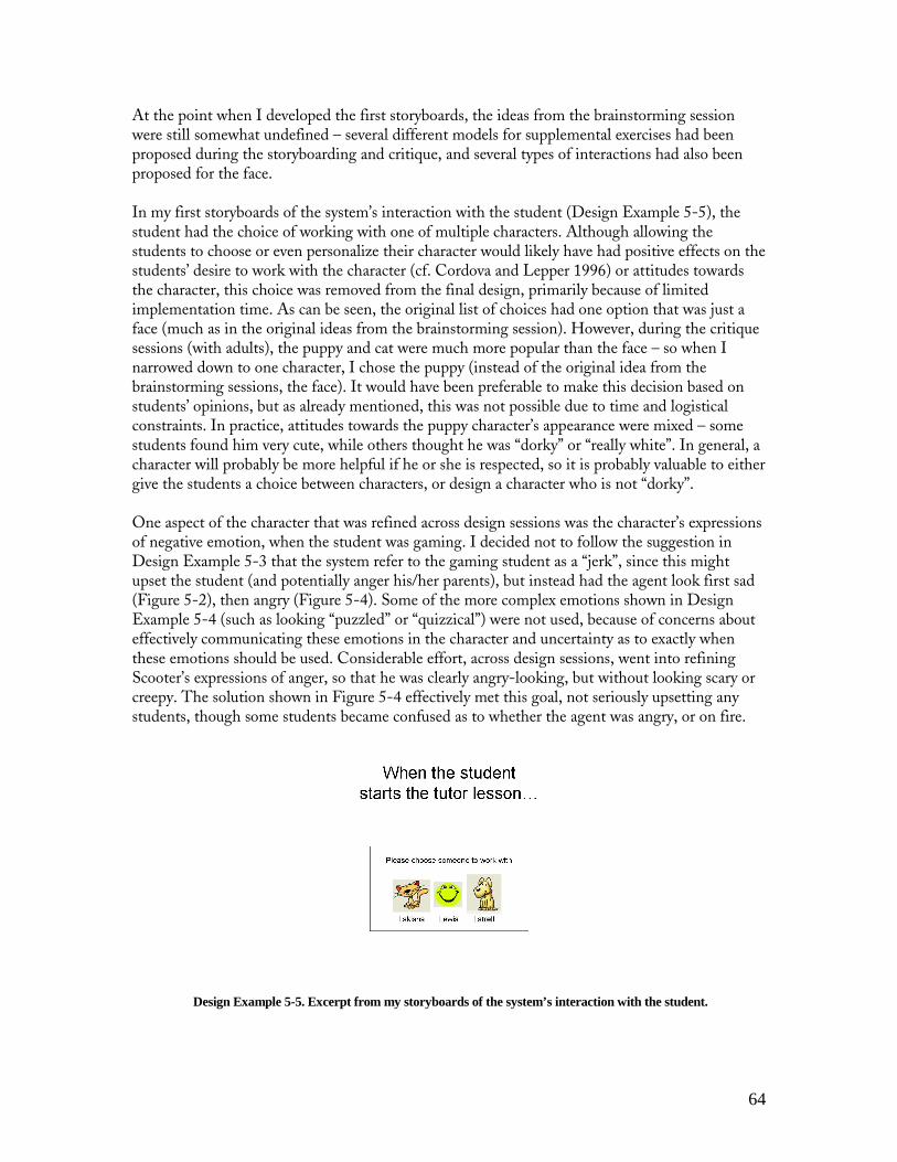
64

At the point when I developed the first storyboards, the ideas from the brainstorming session were still somewhat undefined – several different models for supplemental exercises had been proposed during the storyboarding and critique, and several types of interactions had also been proposed for the face. In my first storyboards of the system’s interaction with the student (Design Example 5-5), the student had the choice of working with one of multiple characters. Although allowing the students to choose or even personalize their character would likely have had positive effects on the students’ desire to work with the character (cf. Cordova and Lepper 1996) or attitudes towards the character, this choice was removed from the final design, primarily because of limited implementation time. As can be seen, the original list of choices had one option that was just a face (much as in the original ideas from the brainstorming session). However, during the critique sessions (with adults), the puppy and cat were much more popular than the face – so when I narrowed down to one character, I chose the puppy (instead of the original idea from the brainstorming sessions, the face). It would have been preferable to make this decision based on students’ opinions, but as already mentioned, this was not possible due to time and logistical constraints. In practice, attitudes towards the puppy character’s appearance were mixed – some students found him very cute, while others thought he was “dorky” or “really white”. In general, a character will probably be more helpful if he or she is respected, so it is probably valuable to either give the students a choice between characters, or design a character who is not “dorky”. One aspect of the character that was refined across design sessions was the character’s expressions of negative emotion, when the student was gaming. I decided not to follow the suggestion in Design Example 5-3 that the system refer to the gaming student as a “jerk”, since this might upset the student (and potentially anger his/her parents), but instead had the agent look first sad (Figure 5-2), then angry (Figure 5-4). Some of the more complex emotions shown in Design Example 5-4 (such as looking “puzzled” or “quizzical”) were not used, because of concerns about effectively communicating these emotions in the character and uncertainty as to exactly when these emotions should be used. Considerable effort, across design sessions, went into refining Scooter’s expressions of anger, so that he was clearly angry-looking, but without looking scary or creepy. The solution shown in Figure 5-4 effectively met this goal, not seriously upsetting any students, though some students became confused as to whether the agent was angry, or on fire.

Design Example 5-5. Excerpt from my storyboards of the system’s interaction with the student.

65

The character’s interaction with the student was, in the final version, simpler than in the some of the original ideas. In some of the design ideas from the brainstorming session, as well as in some of the storyboards (see Design Example 5-6), the character gives specific advice on the student’s gaming actions – advising the student to read through the hint *carefully*, or to try to get the answer right on the first try. However, the gaming detector only gives information as to what steps the student was likely to be gaming on, not exactly how the student gamed – making the generation of an appropriate message non-trivial. An early implementation selected a message at random; when this implementation was being tested, a critiquer pointed out that the messages appeared inappropriate and might cause students to think the system was ineffective, and not take the system seriously. Developing a better alternative, that figured out not just that the student was gaming, but which message was most appropriate, appeared to be potentially fairly time-consuming. Hence, I removed the more specific messages, limiting the character’s comments on gaming to “Work carefully, so you can learn.” (Figure 5-2).

Design Example 5-6. Excerpt from my storyboards of the system’s interaction with the student.

The final design for the supplemental exercises was also somewhat simpler than many solutions suggested during the structured brainstorming session. One popular suggestion during the structured brainstorming session was knowledge construction dialogs, leading the student through each step of the process of determining the answer; however, developing a system that could present sophisticated knowledge construction dialogs is not a simple task (Heffernan, 2001), and seemed to be more complex than necessary. Less sophisticated open-ended items had the risk that they would slow the student considerably – especially if the student was floundering. Therefore, I selected multiple-choice items, which were both easier to implement, and had some bound on how long they would take the student to complete. As can be seen from these examples, the eventual design kept the spirit of the original ideas from the structured brainstorming session, but was fairly different in details from the storyboards produced at the end of the structured brainstorming session. The design process used, with iterations of critique and re-design, refined and improved the original, somewhat abstract designs, bringing their broad ideas and themes into contact with the realities of what can be implemented (in the given time), and testing out how specific features manifest themselves when worked out in detail, and how those features can be improved and refined. Final Design

66

The design which resulted from this process introduced a new component to the students’ intelligent tutoring software – Scooter the Tutor. Scooter was designed to both reduce the incentive to game, and assist students in learning the material that they were avoiding by gaming the system. Scooter was also designed to minimally affect students who were not gaming. Scooter the Tutor is a puppy character, using graphics from the Microsoft Office Assistant (Microsoft Corporation 1997), graphically modified to enable Scooter to display emotions not used in Microsoft Office. Pedagogical agents have been used in several prior educational systems (Mathan and Koedinger 2003; Graesser et al, 2003; Johnson, Rickel, and Lester 2000; Wang et al, 2005). In specific, the Microsoft Office Assistant/ Microsoft Agent has been used in two educational systems (Mathan and Koedinger 2003; Manske and Conati 2005). Multiple studies have, in recent years, suggested that the mere presence of a pedagogical agent does not improve learning but that agents can affect learning positively if used in a fashion that enables new types of educational interactions (Graesser et al, 2003; Wang et al, 2005). Scooter was designed to focus on students who game the system. The gaming detector discussed in Chapter Three (specifically, versions of the detectors trained only on student data from the scatterplot lesson, and from the percents lesson, respectively) is used to assess whether, and to what degree, a student has been gaming the system. If a student is assessed as not having engaged in any gaming recently (in the last 10 actions), Scooter looks happy and gives the student positive messages (Figure 5-1). If the detector assesses that the student may have gamed on 1 of the last 10 actions, Scooter looks upset, and gives the student a warning message (Figure 5-2). When the student is assessed to have been gaming on at least 3 recent actions, Scooter does one of two things, based on whether the student had gotten a correct answer on their last action. If the last answer was correct, Scooter gives the student a set of supplementary exercises designed to give the student another chance to cover the material that the student may have bypassed while gaming the system (Figure 5-3). If the answer was incorrect, Scooter looks angry, to signal to the student that he or she should now stop gaming, and try to get the answer in a more appropriate fashion (Figure 5-4). Scooter also looks angry if a student tries to game him during a supplementary exercise.

Figure 5-1. Scooter the Tutor, when the student has not been gaming

67

Figure 5-2. Scooter the Tutor, looking moderately unhappy when the student is believed

to have been gaming moderately

Figure 5-3. Scooter the Tutor, intervening to give a supplementary exercise to a gaming student

68

Figure 5-4. Scooter the Tutor, looking angry when the student is believed to have been gaming heavily, or attempted to game Scooter during a supplementary exercise (see Figure 5-3)

The supplementary exercises cover the material contained in the steps the student recently gamed through. The supplementary exercises have three levels – all questions given in the supplementary exercises are multiple choice. In each of the first two levels of an exercise, the student is asked to answer one of the following two types of questions:

1. Questions which require understanding one of the concepts required to answer the step the student gamed through (for example: “What kind of variable goes on the Y axis of a Scatterplot?)

2. Questions about what role the step they gamed through plays in the overall process of solving the problem (for example: “Why do we need to know the largest value of height in this part of the problem?”)

If the student gets either the first or second level of the exercise correct, Scooter returns the student to the regular tutor exercise (telling the student “That’s right! Let’s get back to work. Be sure to work through every step carefully.”). The student only gets one chance to answer the first or second level of the exercise. If the student gets both the first and second level of the exercise wrong, he or she is given a third, very easy level. We included this third level, so that students would not flounder indefinitely. The third level items involve a concept relevant to the step the student gamed through, but are very easy (for example: “What is the first value of height in the table?”). If a student gets the third level right, he or she returns to the regular tutor exercise; if a student gets the third level wrong, Scooter assumes that the student was trying to game him, and is more likely to give further interventions on the problem step involved, in the future (see the discussion of how the detector changes its assessments after Scooter’s interventions, near the end of Chapter Three). As an additional note, Scooter did not offer supplementary exercises for problem steps that only involved asymptotic skills: i.e., skills that either all students knew before starting the tutor, or skills not generally learned by students as they used the tutor. The rationale for this design choice was that there would be no gain from giving supplementary exercises on these problem steps, and

69

thus supplementary exercises would waste the student’s time. Therefore, if a student gamed heavily on a step only involving asymptotic skills, Scooter looked angry instead of giving supplementary exercises. My hypothesis, in designing Scooter, was that Scooter would benefit students in three fashions. First, by representing how much the student had been gaming, Scooter would make gaming more accountable – the students’ teachers would be able to know which students had recently been gaming. Additionally, there is evidence that simply informing someone about how often they engage in a problematic behavior can reduce that behavior’s incidence (Sarafino 2001). Second, Scooter was intended to invoke social norms in students (cf. Reeves and Nass 1996) by becoming visibly angry when students gamed a great deal, encouraging the student to use the software more appropriately. While it is not common for software agents to become visibly angry (in fact, Picard (1997) views anger as an example of inappropriate emotion in an affective system), it is a very natural behavior in this context. Human teachers become angry with students who game the system (I will present qualitative data to this effect, later in the chapter). It also seems reasonable to posit that if a student working with a human tutor engaged in the sort of gaming behavior students attempt with our Cognitive Tutors (such as systematically entering every number from 1 to 38), the human tutor would become upset. Therefore, I hypothesized that when Scooter becomes angry, it will invoke social norms, and will lead the student to game the system less. Third, by giving students supplemental exercises targeted to the material the student was gaming through, Scooter gives students another opportunity to learn material they have not learned. Students who game bypass specific material, and if a student games on the same problem step across multiple problems, he or she may never get a chance to learn that material. Hence, Scooter’s supplementary exercises give a student a second chance – and another way – to learn material he or she may otherwise miss entirely. Additionally, it was my hypothesis that these exercises would change the incentive to game – whereas gaming might previously have been seen as a way to avoid work, it would now be seen as leading to extra work.

Study Three The third study I conducted as part of the thesis was the first study which attempted to test the effect of using the gaming detector to intervene when a student gamed. In this study, I contrasted a traditional tutor to a tutor with an animated agent (Scooter) designed to both prevent gaming and offer additional learning support to students who gamed. This study also gave evidence on why students game, discussed in Chapter Four. Methods Study Three took place within 5 classes at 2 schools within the Pittsburgh suburbs. Student ages ranged from approximately 12 to 14. As discussed in Chapter One, all students were participating in a year-long Cognitive Tutor class teaching middle school mathematics, and the study was conducted in the spring semester, after students had used the Cognitive Tutor for long enough to know how to use the tutor in a number of ways. 108 students participated in this study, but there was considerable missing data: not all students were present for all portions of the study, not all students answered all of the questions on the questionnaires, some students’ data had to be

70

discarded for some parts of the study because of material some teachers taught during the study (this will be discussed momentarily) and some students’ log file data was lost due to network outages. The degree of data loss was too large to simply eliminate all students who had some data loss, but the type of data loss did not seem appropriate for imputation (too much dependent-measure data was lost). Therefore, in each analysis, a student will be included if I have all of their data relevant to that analysis. Study Three had two parts. In the first part of the study, students used an unmodified Cognitive Tutor lesson, drawn from their standard curriculum. Half of the students (53% of students present for the relevant parts of the study) worked with a lesson on converting between percents and other mathematical representations; the other half worked with a lesson on creating and interpreting scatterplots of data. We used the first part of the study as both a control condition for the second part of the study, and to study what characteristics are associated with the choice to game, in an unmodified tutor lesson (this aspect of Study Three is discussed in Chapter Four). In the second part of the study, students used a modified Cognitive Tutor lesson, which incorporated Scooter. Scooter was designed, as discussed in the previous section, with two design goals: to reduce gaming, and to give additional support to students who persisted in gaming the system. All students who used the percents lesson in week one used the scatterplot lesson in week two; all students who used the scatterplot lesson in week one used the percents lesson in week two. Thus, in the original design of this study, all students served as both control condition (in week one) and experimental condition (in week two), with tutor lesson counter-balanced between conditions. Unfortunately, at one of the two schools, the teachers decided to cover material relevant to the percents lesson, because of state standards exams, during the same week the experimental condition was being run. Since this might bias in favor of the experimental condition in multiple ways, I will not use data from the percents lesson/experimental condition from that school. This leaves only a relatively small amount of data relevant to the percents lesson/experimental condition. Thus, all discussion of Scooter’s interventions (of any type) will involve only the students who used the scatterplot lesson as their experimental condition. While this data loss was unfortunate, restricting the data set used in analyzing Scooter’s effects makes it possible to draw inferences which are not confounded. For each lesson, the students first viewed conceptual instruction, delivered via a PowerPoint presentation with voiceover and simple animations (shown in Chapter One). In the experimental condition, this PowerPoint also included a brief description of Scooter. Then students completed a pre-test, used the tutor for 80 minutes across multiple class periods (a different number of class periods between schools, but constant within each school), and completed a post-test. Test items were counterbalanced across the pre-test and post-test, and are shown in Appendix B. At the beginning and end of the entire study, students completed a questionnaire on their learning attitudes and beliefs (discussed in Chapter Four), and their attitude towards the tutor (pre-test) or Scooter (post-test), including both Likert scale items (1-6) and one open-ended question, asking for other thoughts or comments on the tutor/Scooter. In Table 5-1, we show the pre-test and post-test items used to compare students’ pre-test attitudes towards the tutor in general, with their post-test attitudes towards Scooter. These items were designed such that they differed only in whether they referred to “the tutor” or “Scooter”, to make comparisons as exact as possible. Post-Test Item Corresponding Pre-Test Item

71

“Scooter treats people as individuals” “The tutor treats people as individuals” “Scooter ignores my feelings” “The tutor ignores my feelings” “I feel that Scooter, in his own unique way, is genuinely concerned about my learning.”

“I feel that the tutor, in its own unique way, is genuinely concerned about my learning.”

“Scooter is friendly” “The tutor is friendly” “Scooter is smart” “The tutor is smart” “I would like it if Scooter was a part of my regular tutor”

“Scooter is irritable” “Scooter wants me to do well in class”

Table 5-1. Items used within the Study Three questionnaire, to assess the students’ attitudes towards Scooter.

In addition to the pre-test and post-test measures, I obtained log files, which I used to distill several measures of Scooter’s interactions with each student, including the frequency with which Scooter got angry, and the frequency with which Scooter gave a student supplementary exercises. Finally, I collected observational data on each student’s frequency of gaming, using the same quantitative observational method and observers as in Studies One and Two (see Chapter Two). Deciding what to use to measure gaming in this study is a difficult decision, since both human observation (Chapter Two) and the gaming detector (Chapter Three) have considerable disadvantages in this situation. The human observations have the serious drawback that they cannot distinguish harmful gaming from non-harmful gaming; I cannot even use pre-post gains to classify students into these categories, since the intervention may have improved some the learning of some students in the harmful gaming category, making them appear to be engaging in non-harmful gaming. Thus, if I use the human observations, I will be conflating two types of gaming. At the same time, if I use detector, I will be using the same measure to both drive intervention and as a measure of the intervention’s effectiveness, probably introducing bias into analyses (if the gaming detector only catches half of the types of harmful gaming behavior, and half of harmful gaming students completely desist in that type of gaming behavior, but continue in all other types of harmful gaming, then my detector would say that the number of students seen gaming harmfully decreased by 50%, whereas actually all students continued to game harmfully but some did so less frequently). Because of the potential bias introduced by using the gaming detector, in this study I will use data from the human observers as the measure of gaming. I will address the possibility that the effects on observed gaming frequency came from changes in non-harmful gaming in the Results section. Results The first and most immediately noticeable effect of incorporating Scooter in the tutor was a sizeable, though only marginally significant, reduction in the frequency of observed gaming. Students who used the scatterplot lesson as their control condition gamed an average of 5.5% of the time within that lesson, while students who used the scatterplot lesson as their experimental condition gamed an average of 2.4% of the time within that lesson, t(100)=1.86, p=0.07, effect size = 0.49σ. Interestingly, this drop appeared to occur as a drop in the number of students seen gaming in each condition, rather than as a drop in the rate at which the remaining gaming students gamed. 33% of students were seen gaming in the scatterplot/ control condition, while 18% of students were seen gaming in the scatterplot/ experimental condition, a marginally

72

significant difference, χ2(1,N=102)= 3.30, p=0.07.10 The average gamer in the scatterplot/ control condition gamed 17% of the time, while the average gamer in the scatterplot/ experimental condition gamed 14% of the time, which was not a significant difference, t(23)=0.74, p=0.47. Of course, the reduction in gaming might have been in non-harmful gaming; I will address this possibility later in this section.

% of students ever seen gaming

0

5

10

15

20

25

30

35

Control Experimental

Figure 5-5. The occurrence of gaming (observed) in each condition, for the Scatterplot lesson.

Despite the apparent reduction in gaming, however, there was not an apparent improvement in learning. Overall, students in the scatterplot/control condition scored 44% on the pre-test and 66% on the post-test, a 22 point gain, whereas students in the scatterplot/experimental condition scored 37% on the pre-test and 62% on the post-test, a 25 point gain. The difference in students’ gains between conditions was not significant, t(70)=0.34, p=0.73. There was the appearance of a difference in the relationship between pre-test and post-test between the two conditions; as can be seen in Figure 5-6, students who scored between 0% and 50% on the pre-test appear to have done better on the post-test in the experimental condition, with the difference largest (15 points) among those students who scored 0% on the pre-test. However, the aptitude-treatment interaction was not significant, F(1,69)=1.71, p=0.20.

10 To put these frequencies into context, 24% of students were observed gaming in either fashion in Study One, and 41% of students were observed gaming in either fashion in Study Two.

73

0

0.1

0.2

0.3

0.4

0.5

0.6

0.7

0.8

0.9

1

0 0.2 0.4 0.6 0.8 1

pre

po

st control

exp

Figure 5-6. The relationship between pre-test and post-test in each condition (only data from the Scatterplot lesson is shown, for best comparability).

However, gamers are a small subset of the overall population – therefore, differences in gamers’ learning may be swamped by normal variation in the rest of the population. Only a third of students were ever observed gaming in the control condition – and moreover, the gaming detector and interventions are designed for a specific subset of this subset. Interestingly, the relationship between gaming and post-test performance even appears to switch direction between conditions, as shown in Figure 5-7. In the control condition, more gaming is associated with poorer learning, as in Study One (see Chapter Two); in the experimental condition, by contrast, more gaming actually appears to be associated with more learning – though the interaction effect between the effects of gaming and the condition is not significant, F(1,81)=1.84, p=0.18. It is worth noting, by the way, that this trend (or lack of a trend) is evidence that the reduction in observed gaming did not come from reducing the frequency of non-harmful gaming with no reduction in harmful gaming. If that had been the case, we would expect gaming to be much more strongly associated with poorer learning in the experimental condition, which was not the case.

74

0

0.1

0.2

0.3

0.4

0.5

0.6

0.7

0.8

0.9

1

0 0.05 0.1 0.15 0.2 0.25 0.3

Gaming pct

Po

st-t

est

Control

Exp

Figure 5-7. The relationship between gaming and post-test, in each condition (best-fit lines are shown rather than empirical data, for comprehensibility).

Hence, Scooter appears to have had an overall effect on gaming, but not on learning (though there was a trend towards greater learning). However, not all gaming students received the same number of Scooter’s interventions. Hence, it may be worth looking at the students who got the most interventions from Scooter, to see how/if their gaming behavior and learning was affected by Scooter. In the following sections, I will examine the behavioral and learning outcomes associated with each type of intervention, analyzing the two types of interventions separately, since the two types of interventions were given in subtly different situations and may have had different effects. Scooter’s Supplementary Exercises In this section, I will examine the outcomes associated with Scooter’s supplementary exercises (an example exercise is shown in Figure 5-3). Scooter gave a fairly small number of exercises. No student received a set of exercises from Scooter on more than 3.2% of problem steps (12 sets), the median student received a set of exercises on 1.1% of problem steps (3 sets), and many students received no exercises at all. But, on the other hand, Scooter’s exercises were assigned to exactly the problem steps students gamed on (according to the detector), so the exercises might have disproportionate effects on learning. One possible model for how learning could relate to number of supplementary exercises received is that there could be a linear relationship – the more supplementary exercises a student receives, the more they learn. However, a linear model ignores the fact that the students who never receive supplementary exercises don’t receive supplementary exercises because they don’t engage in harmful gaming, and that not engaging in harmful gaming is generally associated with better learning (see Chapter Two). Therefore, it may be more reasonable to expect the relationship between supplementary exercises and learning to be as follows: students who receive no supplementary exercises show good learning, students who receive many supplementary exercises show good learning, and the

75

students in the middle show poorer learning. In fact, this is exactly the relationship we find, shown in Figure 5-8.

Figure 5-8. The Learning Gains Associated With Receiving Different Levels of Supplemental Exercises From Scooter

(Empirical data shown) The third of students that received the most supplementary exercises had significantly better learning than the other two thirds, t(37)=2.25, p=0.03; the overall difference between all three groups is also significant, F(2,36)=3.10, p=0.06. Hence, it appears that the students who received the most supplementary exercises learned more than the other students in the class. In the remainder of the section, I will analyze this finding in more depth. However, before doing so, I will first consider whether there is a more meaningful place to split between groups than the 67th percentile. To do so, I will develop a model of the relationship between supplemental exercises and learning gains. The empirical relationship between these quantities is shown in Figure 5-9, in a more broken-down form.

76

Figure 5-9. The Learning Gains Associated With Receiving Different Levels of Supplemental Exercises From Scooter

(Empirical data shown) (5th quartile did worse on post-test than pre-test)

Given the relationship we can see in Figure 5-9, it is not surprising that a linear function does a poor job of modeling the relationship between pre-post gain and the number of supplemental exercises, achieving an r2 of 0.02. A reverse bell-curve also does a poor job – a quadratic function does not even converge as a reverse bell-curve, instead converging to a nearly linear positive relationship which also has an r2 of 0.02 (2 parameters). A “V” function (segmented regression with a single split, 3 parameters) achieves an r2 of 0.10, which is still not very good. A bimodal model (segmented regression on quadratic functions with a single split, 5 parameters), however, achieves a substantially better r2 of 0.36. The improved fit given by the bimodal model does not simply appear to be the result of adding

more parameters. The bimodal model achieves a BIC' of 0.64, whereas the best-fitting model

which treats this relationship as a linear function achieves a BIC' of 2.98, and the best-fitting “V”

model achieves a BIC' of 6.82. Hence, the difference in BIC' between the bimodal and linear

models is 2.34, which is equivalent to a p-value of 0.02 (Raftery 1995), and the difference in BIC' between the bimodal and “V” models is 6.18, which is equivalent to a p-value of 0.003. Hence, a bimodal model appears to be more appropriate to the data than other potential models. The best-fitting bimodal model states that the expected pre-post gain equals (giving P for the percentage of steps where the student received a set of supplemental exercises): If P<0.0122, 0.63 – 62.91P + 12553.13P 2

If P �0.0122, 1.83 – 66.24P + 3507.28P 2

This function can also be written (somewhat more comprehensibly) as:

If P<0.0122, 0.31 – 12553.13*(0.005-P) 2

If P �0.0122, 0.57 – 3507.28 *(0.019-P) 2

In this model, 0.31 and 0.57 represent the two modes’ Y-values, and 0.005 and 0.019 represent the two modes’ X-values. 0.0122 represents the most likely split-point between the two halves of

77

the distribution: when the student receives a supplementary exercise 1.22% of the time (the 63rd percentile). The graph of the relationship given by the bimodal model is shown in Figure 5-10.

0

0.1

0.2

0.3

0.4

0.5

0.6

0.7

0 0.5 1 1.5 2 2.5 3 3.5

Supplemental Exercises (% frequency)

Pre

-Po

st G

ain

(m

od

el)

Figure 5-10. The Learning Gains Associated With Receiving Different Levels of Supplemental Exercises From Scooter

(Predictions from best-fitting bimodal model shown)

We can now use the division between the two halves of the bimodal model (supplemental exercises = 1.22%) to divide the students into a group of students who received many supplemental exercises group, and a group of students who received fewer supplemental exercises. The students who received many supplemental exercises have an average pre-post gain of 46%, compared to an average pre-post gain of 11% for the students who received fewer exercises, t(37)=2.48, p=0.02, effect size = 0.79σ. To look at the difference another way, although the students who received many exercises were substantially lower at pre-test (20% versus 53%), the two groups were essentially equal by the post-test (66% versus 64%), as shown in Figure 5-11. The interaction effect is statistically significant, F(1,37)=6.16, p=0.02, for a repeated-measures ANOVA. It is also important to note that there is not a ceiling at 66%: 28% of all students (33% of students in the top 3 eighths, 25% of the other students) had perfect scores on the post-test; there is also not a post-test floor effect – some students in each groups had low post-test scores.

78

0

10

20

30

40

50

60

70

pre post

Sco

re more exercises

fewer exercises

Figure 5-11. The Learning Gains Associated With Receiving Different Levels of Supplemental Exercises From Scooter

That said, students with lower pre-test scores could be expected to catch up to students with higher pre-test scores, in some situations (for example, if most students knew skills A,B, and C after using the tutor but many students did not know all of these skills before using the tutor), and it’s possible that the effect we’re observing could be explained in this fashion. One way to investigate this possibility would be to compare students with low pre-test scores in each group – this step, however, substantially reduces sample size and therefore strongly biases any statistical comparison towards non-significance. There is another way to investigate this possibility, without drastically reducing sample size: comparing each group of students’ actual gains to the gains that we could have expected they would gain. We can figure out a baseline amount we expect each student to gain, using data from the control condition to fit an expected function between each student’s pre-test and post-test. The best-fitting function for the control condition data (with an r2 of 0.25 to the actual data in that condition) is

Post-Test = 0.44 + (0.56)Pre-Test If we predict each experimental-condition student’s post-test using this formula, we find that according to this prediction, the students who received more supplementary exercises could have been expected to perform 19 percentage points worse on the post-test than the students who received fewer supplementary exercises. Instead, however, the students who received more supplementary exercises performed 2 percentage points better on the post-test than the students who received fewer supplementary exercises. In other words, the students who received the most supplementary exercises gained 21 more points relative to the other students than predicted, a marginally significant difference, t(37)=1.71, p=0.09 for a two-tailed t-test. Hence, it appears that the pattern shown in Figure 5-11 can not be explained as all students with low pre-test scores catching up to the rest of the class. Instead, it appears that students who received the most supplementary exercises learned more than the other students, and this greater learning enabled them to catch up to the rest of the class. It’s also worth noting that this pattern

79

is the exact opposite of the one seen in the earlier studies of gaming’s effects on learning (see Chapter Two), where students who frequently gamed started behind the rest of the class and fell further behind by the post-test, rather than catching up, as the students who receive many supplementary exercises do. Interestingly, however, though there appears to be a connection between receiving more exercises from Scooter and increased learning, Scooter’s exercises do not appear to have led to the decrease in gaming reported in the previous section. If Scooter’s exercises directly led students to reduce their gaming, we would expect the students who received more exercises to reduce their gaming over time. There is no evidence of such a decrease. Figure 5-12 shows the frequency in gaming over the 3 days of the study among the students who received many exercises received in the scatterplot/experimental condition, compared to the students who received fewer exercises. Among the students who received more exercises, neither the apparent increase in gaming from day 1 (7%) to day 2 (10%), nor the apparent decrease in gaming from day 2 (10%) to day 3 (7%), was statistically significant, χ2(1,N=155)= 0.31, p=0.58, χ2(1,N=105)= 0.17, p=0.68. Overall, the students who received more exercises gamed significantly more than the students who received fewer exercises, χ2(1,N=388)= 24.33, p<0.001.

Observed Gaming

0

2

4

6

8

10

12

1 2 3

Day

% G

amin

g

High Interventions

Others

Figure 5-12. Gaming Over Time, in the Scatterplot/Experimental Condition

Case Studies In this section, I will present a pair of case studies to put some of the effects observed in this study into context. Specifically, I will compare a pair of high-gaming students, one in the scatterplot/experimental condition, and the other in the scatterplot/control condition – and show how Scooter changed the student’s experience in the scatterplot/experimental condition. Experimental Condition

80

“Chris” (not his/her real name; also, gender was not recorded in this study) was a 9th-grade student. Chris had a low pre-test score (17%) and a high post-test score (100%). On the pre-test, Chris demonstrated a common misconception (cf. Baker, Corbett, and Koedinger 2001), where students select variables which would be more appropriate for a bar graph than a scatterplot (one categorical variable and one quantitative variable); however, for the one correct variable, Chris selected an appropriate scale and bounds. Chris plotted points, but they were not evaluated (in accordance with a repeatedly-used grading policy for the scatterplot lesson’s tests), since plotting values along categorical variables is not necessarily the same as plotting values along quantitative variables. On the post-test, Chris performed perfectly. Chris’s graph had the correct two variables, both of the correct type (quantitative). Both axes had an appropriate scale, and all points were plotted correctly. Chris was observed gaming 10% of the time in the experimental condition (in the 91st percentile of all students), and received supplementary exercises on 2.4% of problem steps (also in the 91st percentile of all students). In absolute terms, Chris received 9 sets of supplementary exercises in the 66 minutes he used the tutor. 6 of those 9 sets of exercises directly concerned how to tell the difference between what types of variables should be used in scatterplots and what types of variables should be used in bar graphs, or concerned the actual step of choosing which variable to use in the graph. In other words, Chris received a small number of exercises, but these exercises were focused exactly on the skill he most needed to learn – and he learned that skill. (Point plotting, which Chris also appeared to learn from pre-test to post-test, is learned all students by the time they have plotted a small number of points – Baker, Corbett, Koedinger, and Schneider 2003). Interestingly, after showing impressive learning gains, Chris wrote on the post-test (on the open-ended response question) that “Scooter can be very annoying. Please do not put him on regular tutor” – indicating that, although Chris had impressive learning – quite likely due to using Scooter – Chris disliked Scooter. Control Condition “Pat” was a 9th-grade student. Like Chris, Pat had a low pre-test score (0%), but unlike Chris, Pat had a low post-test score (17%). Like Chris, Pat demonstrated a common misconception on the pre-test where students select variables which would be more appropriate for a bar graph than a scatterplot (one categorical variable and one quantitative variable). For the one correct variable, Pat made a related misconception, treating a quantitative variable as if it were a categorical variable. Like Chris, Pat plotted points, but they were not evaluated (in accordance with a repeatedly-used grading policy for the scatterplot lesson’s tests), since plotting values along categorical variables is not necessarily the same as plotting values along quantitative variables. On the post-test, Pat showed only moderate improvement over the pre-test. Like on the pre-test, Pat selected variables which would be more appropriate for a bar graph than a scatterplot (one categorical variable and one quantitative variable). However, on the post-test, Pat selected an appropriate scale and bounds for the one correct variable, avoiding the earlier error where Pat treated a quantitative variable as if it were categorical.

81

Pat was observed gaming 10% of the time in the experimental condition, exactly the same proportion of the time as Chris – although in this lesson 10% gaming was only in the 71st percentile of all students. Pat was never seen gaming on the problem steps where it is possible to treat a quantitative variable as nominal – and never made this error on the post-test. Pat gamed 19 times11 (or 4.75 times per problem completed) on the problem steps which directly concerned how to tell the difference between what types of variables should be used in scatterplots and what types of variables should be used in bar graphs, or concerned the actual step of choosing which variable to use in the graph. Therefore, had Pat been in the experimental condition, it seems likely he/she would have received some number of supplementary exercises on these skills. As Pat was in the control condition, however, he/she did not receive any supplementary exercises. Hence, Pat made a variable choice error on the pre-test, gamed on the steps which would have taught him the relevant skill, and made the same error on the post-test. Chris made the exact same error on the pre-test, and gamed on the steps which would have taught him the relevant skills – but then Chris received 9 sets of supplementary exercises on these skills, and avoided the error on the post-test. This provides some illustration on how a small number of supplementary exercises could be associated with substantial learning gains – they were targeted by the gaming detector towards exactly the steps that students were avoiding learning by gaming. Scooter’s Expressions of Displeasure In this section, I will examine the outcomes associated with Scooter becoming angry (a example is shown in Figure 5-4). Scooter became angry considerably more often than he gave supplementary exercises. The median student saw an angry Scooter 12.5% of the time, and the student who saw an angry Scooter the most often saw an angry Scooter 38% of the time. There did not appear to be a strong association between viewing an angry Scooter more often, and better learning. Although there was some appearance of a trend towards greater learning for students who received more expressions of anger from Scooter (see Figure 5-13), there was neither a significant linear relationship between expressions of anger and learning, t(39)=0.32, p=0.75, nor did students who received the most expressions of anger have a significantly larger average learning gain than other students, t(37)=0.48, p=0.63, effect size = 0.20σ comparing the top quartile to the other students.12

11 Using the same detector used in the experimental condition

12 If we select a different cutoff point, it does not change significance; for the top 3/8 versus the other 5/8, t(37)=0.41, p=0.68; for a median split, t(37)=0.15, p=0.88; for the top third versus the other two thirds, t(37)=0.16, p=0.87.

82

Figure 5-13. The Learning Gains Associated With Receiving

Different Levels of Expressions of Anger From Scooter.

Additionally, there is no evidence of a relationship between Scooter’s frequency of expressions of anger, and a reduction in gaming over time. Figure 5-13 shows the frequency in gaming over the 3 days of the study among the top quartile of students (in terms of seeing an angry Scooter) in the scatterplot/experimental condition, compared to the other students in this condition. As Figure 5-11 shows, neither group of students substantially changed their gaming over the course of the study. Among the students who saw an angry Scooter the most often, neither the apparent decrease in gaming from day 1 (7%) to day 2 (6%), nor the apparent increase in gaming from day 2 (6%) to day 3 (13%), was statistically significant, χ2(1,N=79)= 0.04, p=0.84, χ2(1,N=50)= 0.83, p=0.36.

Observed Gaming

0

2

4

6

8

10

12

14

1 2 3

Day

% G

amin

g

More Angry Scooter

Less Angry Scooter

Figure 5-13. Gaming Over Time, in the Scatterplot/Experimental Condition

83

Why Did Gaming Reduce? As mentioned earlier in this chapter, there was a (marginally significant) overall reduction in gaming in the condition where Scooter is present. However, neither students who saw an angry Scooter more often nor students who received more supplementary exercises reduced their gaming over time. It is possible that simply knowing Scooter was present, and that he would look unhappy when students gamed, and that the teacher would see Scooter, was sufficient to explain the reduction in gaming from the control condition to the experimental condition. Students who were less committed to gaming might not want to game if they knew their teacher would know. Thus, although Scooter’s mood may not have directly affected the students who saw an angry Scooter, Scooter’s presence may have motivated students to avoid gaming during the entire lesson. Student Attitudes Towards Scooter

At this point, we know that Scooter had positive effects towards reducing gaming, and appeared to improve some students’ learning through his supplementary exercises. These elements suggest that Scooter was a useful and positive addition to the classroom experience. However, it is also important to consider whether the students found working with Scooter a positive experience. In this section, I will examine data on students’ attitudes towards Scooter, in comparison to their attitudes to the regular tutor (before using Scooter). Since most students enjoy working with the tutor (Schofield 1995; Baker, Roll, Corbett, and Koedinger 2005), this should be a reasonably strong comparison.

In doing so, I will consider three groups of students’ attitudes towards Scooter: students who received considerable numbers of supplemental exercises (the set of students who were identified as having received more supplemental exercises, earlier in this chapter), students who received considerable numbers of expressions of anger from Scooter, and students who were in neither of these groups (and therefore primarily saw a dancing, happy Scooter).

It’s reasonable to expect that there will be pre-test differences between these groups (since, as discussed in Chapter Four, one of the factors that leads to gaming is disliking the tutor) – therefore, the goal of this section will not be to compare these three groups of students to each other (which is likely to lead to the unsurprising result that students who see a happy dancing puppy enjoy that more than seeing an angry, critical puppy), but to see how each of these three groups of students liked Scooter, in comparison to their regular tutor.

All of the items that I will discuss in this section involve Likert scales, from 1 to 6. For the majority of items, 1 indicated “Strongly Disagree” and 6 indicated “Strongly Agree” – I will explicitly indicate cases where the scale is reversed. On all items, the middle possible average response is 3.5 – however, each student individually needed to indicate 3 or 4. Student Attitudes Towards Scooter –Students Who Received Many Supplementary Exercises The students who received a considerable number of supplementary exercises from Scooter were neutral to negative towards Scooter. These students had an average response of 2.9 to the question “I would like it if Scooter was a part of my regular tutor” (with a 95% confidence band of 1.8-3.9, encompassing the middle possible value, 3.5).

84

However, across the five items that compared Scooter to the tutor, there was a significant trend towards students’ attitudes towards Scooter being lower than their pre-test attitudes towards the tutor, t(13) = 2.78, p=0.02, for a two-tailed paired t-test. The students’ average pre-test rating of the tutor was 3.9 and their average post-test rating of Scooter was 3.0.

The students who received more supplementary exercises rated Scooter lower than their regular tutor on the items asking whether Scooter/the tutor treats people as individuals, t(13) =2.22, p=0.05, for a paired t-test, whether Scooter/the tutor is smart, t(13)=4.94, p<0.001, for a paired t-test, and whether Scooter/the tutor is friendly, t(13)=2.39, p=0.03. It is surprising that these students gave Scooter low ratings on being smart and treating students like individuals, since Scooter was using assessments of individual differences in order to offer what turned out to be highly effective adaptations to these very students – hence, one might say that Scooter actually was smart and was treating people as individuals. Nonetheless, these results suggest that even if Scooter succeeded in these goals, it was not apparent to the very students who benefited. It may be interesting to investigate, in a followup study, what these students attribute their learning to in this lesson.

The other two items did not decrease significantly. The overall pattern of responses of the students who received the most supplementary exercises is shown in Table 5-2. Test Item

Pre-Test Mean Post-Test Mean Statistical Significance (p)

“The tutor/Scooter is smart” 4.9 3.1 <0.001 “The tutor/Scooter treats people as individuals” 3.8 3 0.05 “The tutor/Scooter ignores my feelings” (item goes in opposite direction to others)

3.2 3.5 0.27

“The tutor/Scooter is friendly” 3.9 2.9 0.03 “I feel that the tutor/Scooter, in its/his own unique way, is genuinely concerned about my learning.”

3.6 3.3 0.36

“Scooter is irritable.” n/a 3.9 n/a

“I would like it if Scooter was part of my regular tutor.”

n/a 2.9 n/a

Table 5-2. Differences between pre-test attitudes towards the tutor, and post-test attitudes towards Scooter, among the students who received the most supplementary exercises (top 3/8)

Student Attitudes Towards Scooter –Students Who Frequently Saw an Angry Scooter The students who saw an angry Scooter the most often (the top quartile in the scatterplot/ experimental condition) were also very displeased with some aspects of Scooter, but – interestingly – different aspects than the students who received the most supplementary exercises. These students had a mean response of 3.6 to the question “I would like it if Scooter was a part of my regular tutor” – exactly in the middle of the possible response range. However, there is evidence that these students had a generally low opinion of Scooter. These students tended to agree with the sentence “Scooter is irritable” (average response of 4.7, 95% confidence band=4.0-5.4, significantly different than chance). Additionally, across the five items that compared Scooter to the tutor, there was a significant trend towards students’ attitudes towards Scooter being lower than these students’ pre-test attitudes towards the tutor, t(6)=2.79, p=0.03, for a paired t-test. The students’ average pre-test rating of the tutor was 3.7 and their average post-test rating of Scooter was 2.3.

85

These students trended towards rating Scooter lower than the tutor on each of the five comparison items. The trend was statistically significant for their opinions of Scooter’s intelligence, t(7)=4.46, p<0.01, for a paired t-test, and whether Scooter ignored their feelings, t(7)= -3.86, p<0.01, for a paired t-test. The trend was marginally significant – or nearly so – for the other three items, t(6) = 1.80, p=0.12, t(7) = 1.69, p=0.14, t(7)=1.95, p=0.10. The overall pattern of responses of the students who received the most supplementary exercises is shown in Table 5-3. Test Item

Pre-Test Mean Post-Test Mean Statistical Significance (p)

“The tutor/Scooter is smart” 5.3 2.9 <0.01 “The tutor/Scooter treats people as individuals” 4.6 3.4 0.12 “The tutor/Scooter ignores my feelings” (item goes in opposite direction to others)

3.3 4.1 <0.01

“The tutor/Scooter is friendly” 4.5 3.4 0.14 “I feel that the tutor/Scooter, in his/its own unique way, is genuinely concerned about my learning.”

4.4 3 0.10

“Scooter is irritable.” n/a 4.7 n/a

“I would like it if Scooter was part of my regular tutor.”

n/a 3.6 n/a

Table 5-3. Differences between pre-test attitudes towards the tutor, and post-test attitudes towards Scooter, among the students who saw an angry Scooter the most often (top quartile)

Student Attitudes Towards Scooter – Other Students The students who neither saw an angry Scooter the most often nor received the most supplementary exercises were overwhelmingly neutral towards Scooter. These students had a mean response of 3.6 to the question “I would like it if Scooter was a part of my regular tutor” – exactly in the middle of the possible response range. These students tended to agree with the sentence “Scooter is irritable” (average response of 4.2, 95% confidence band=3.6-4.8, significantly different than chance). However, across the five items that compared Scooter to the tutor, there was not a significant trend towards students’ attitudes towards Scooter being lower than these students’ pre-test attitudes towards the tutor, t(19)=1.29, p=0.21, for a paired t-test.

These students rated Scooter lower than their regular tutor on the items asking whether Scooter/the tutor is smart, t(18) =2.05, p=0.06, for a paired t-test. The other four items did not decrease significantly. The overall pattern of responses of these students is shown in Table 5-4.

86

Test Item

Pre-Test Mean Post-Test Mean Statistical Significance (p)

“The tutor/Scooter is smart” 4.8 4.1 0.06 “The tutor/Scooter treats people as individuals” 4.4 4.0 0.29 “The tutor/Scooter ignores my feelings” (item goes in opposite direction to others)

3.4 3.5 0.73

“The tutor/Scooter is friendly” 4.4 3.9 0.31 “I feel that the tutor/Scooter, in his/its own unique way, is genuinely concerned about my learning.”

3.9 4 0.99

“Scooter is irritable.” n/a 4.2 n/a

“I would like it if Scooter was part of my regular tutor.”

n/a 3.6 n/a

Table 5-4. Differences between pre-test attitudes towards the tutor, and post-test attitudes towards Scooter, among the students who did not receive the most supplemental exercises, or see an angry Scooter the most often. Student Attitudes Towards Scooter – Summary Overall, then, the students whose experiences were most substantially affected by Scooter appear to have liked him least. The trend towards disliking Scooter was moderately more pronounced among those students who saw an angry Scooter the most often (by comparison to the students who saw the most supplementary exercises). Hence, although Scooter had positive effects towards reducing gaming, and appeared to improve some students’ learning through his supplementary exercises, there is considerable room for improvement in making working with Scooter a more enjoyable, positive experience. On the other hand, the students who did not see an angry Scooter very often or receive many supplementary exercises were more or less neutral towards Scooter. This finding suggests that, at minimum, this design fulfilled the second solution parameter identified at the beginning of this chapter -- change the tutor minimally for students who do not game. Thus, this design can be considered a reasonable success. The students who received many supplemental exercises appear to have had better learning, though they disliked several aspects of Scooter. The students who received few interventions (of either type) from Scooter were largely unaffected, in either learning or attitudes. Only the students who received many expressions of anger from Scooter appeared to have had their experience with the tutor changed for the worse – and even these students, while they did not enjoy working with Scooter, did not appear to have learned less than other students. This outcome does, however, suggest that perhaps future versions of Scooter should retain his supplemental exercises while finding a less irritating way to communicate to the student and their teacher that the student has been gaming.

Contributions There are two contributions from this chapter of the thesis. The first contribution is obvious and direct. In this chapter, I have presented a re-designed tutor which reduces the number of students who game and enables gaming students who receive many supplementary exercises to catch up to the rest of the class. The re-designed lesson presented is not without flaws – most importantly, the students who most benefited from the system tended to like it less than their regular tutor. It will be important to investigate if Scooter can be made more likeable without reducing his educational effectiveness.

87

It will also be worthwhile to explore Scooter’s design further. For example, the reduction in gaming did not appear to be associated with the learning gains some students saw. It may be more effective, in future design iterations, to try to not reduce gaming, so that we can better see which students would benefit from supplementary exercises (this approach treats gaming not as a problem in itself, but as a sign that the student needs help). It may also be possible to detect when non-gaming students could benefit from supplementary exercises (it might be of value, for instance to give supplemental exercises on any step where the student had had difficulty across several problems, regardless of whether the student gamed the system). This chapter makes a second contribution, having to do with process. In this chapter, I presented a system which was reasonably successful on its very first deployment, despite addressing an issue in student learning in interactive learning environments that had largely not been previously addressed. I believe that such rapid success can only be explained by good design process. Most of the original hypotheses (from our group, and other researchers) for what behaviors should be connected with poorer learning (Chapter Two) and for why students game (Chapter Four), were completely incorrect (at least within the learning environment studied), and therefore probably would have led to the design of useless or even counterproductive systems. The extensive research I conducted at the beginning of the design cycle (detailed in Chapters Two and Four) prevented such an error. Additionally, my early ideas for how to respond to gaming, even though informed by the research in those chapters, seem, in retrospect, substantially flawed in comparison to the design used in Study Three. In this chapter, I show how structured brainstorming (with a diverse and enthusiastic group of experts) and repeated prototype-and-critique cycles helped me to considerably improve the design of the system presented in Study Three. The exact contributions of good design process can be difficult to articulate – it’s not possible to run a controlled experiment where the same designer or designers either follow good process or fail to do so. Nonetheless, a design process can be judged by what it produces – and the system presented here, though far from perfect, appears to have been a reasonable success.

88

Chapter Six Conclusions and Future Work

This thesis makes a number of contributions, across several fields. In this chapter, I will summarize these contributions, and discuss some future directions for the program of research presented in this dissertation.

Human-Computer Interaction: How Do Student Decisions When Using Educational Systems Affect Their Learning? Findings It has been known for some time that students who use a variety of types of educational technology game the system, attempting to succeed in an educational environment by exploiting properties of the system rather than by learning the material and trying to use that knowledge to answer correctly. In this thesis I establish that only a minority of students game the system, but that the choice to game the system is associated with considerably poorer learning than other seemingly non-productive behaviors, such as talking off-task. I also establish, however, that not all types of gaming are associated with equally poor learning outcomes, showing that gaming behavior within the intelligent tutoring system studied divides into “harmful gaming” and “non-harmful gaming”, and that these two types of gaming are automatically distinguished by machine learning. Techniques To establish these findings, I used a pair of techniques which are likely to be useful for detecting and modeling other types of student behavior. The first technique is quantitative field observation. Quantitative field observation has a rich history in the behavioral psychology literature (Lahaderne 1968; Karweit and Slavin 1982; Lloyd and Loper 1986; Lee, Kelly, and Nyre 1999). The method I use in this dissertation adapts this technique to the study of behavior in interactive learning environments, changing the technique in a seemingly small but useful fashion: Within the method I use in this dissertation, the observer codes for multiple behaviors rather than just one. Although this may seem a small modification, this change makes this method useful for differentiating between the learning impact of multiple behaviors, rather than just identifying characteristics of a single behavior. The method for quantitative field observations used in this dissertation achieves good inter-rater reliability, and has now been used to study behavior in at least two other intelligent tutor projects (Nogry 2005; Neil Heffernan, personal communication). The data from quantitative observation becomes even more useful, I have found, when analyzed with a psychometrically-inspired machine learning framework – in this case, a Latent Response

89

Model. Learning Latent Response Models from the data enabled me to differentiate between two types of gaming which were indistinguishable to human observers. The model also made more precise predictions about how often each student gamed the system.

Machine Learning: Developing Detectors of Student Behavior Findings In this dissertation, I present a gaming detector that verifiably works on a number of tutor lessons, and which can be used to detect gaming within new tutor lessons without large degradations in performance. This work establishes that is possible to develop a behavior detector that can transfer effectively between fairly different lessons within-curriculum. The results presented here also suggest that it is beneficial to train on multiple lessons, to obtain a detector which can be generalized to lessons beyond the original training lessons. Techniques In order to develop this detector, I adapted a psychometric framework, Latent Response Models, for use in machine-learned behavior detection. LRMs have a number of advantages for behavior detection, being able to naturally take advantage of multiple sources of data at different grain-sizes. My work in adapting LRMs to this task involved developing a new type of three-level LRM, and inventing a new algorithm – based on forward selection, iterative gradient descent, and Fast Correlation-Based Filtering, to search the space of potential LRMs. The techniques I developed for learning LRMs have proved useful not just in developing a detector of gaming, but have also proven useful for mining information about other types of behavior in Cognitive Tutor log files. I believe that LRMs will be useful in a considerable range of behavior detection and data mining problems – essentially, whenever there is fine-grained data from log files that can be combined with aggregate, user-by-user data.

Educational Psychology: What Distinguishes the Students who Choose to Game the System? Findings In this dissertation, I presented three studies which give data on what behaviors, attributes, motivations, and beliefs characterize the students who choose to game. I use this data to develop a profile of a prototypical gaming student, which I use in Study Three to develop an intervention which responds (reasonably) appropriately to gaming. This profile shows that gaming students have a consistent pattern of disliking virtually every aspect of their classroom environment, and are generally not self-driven, across educational contexts; however, these students do not have a goal of performing well in the tutor instead of learning (contrary to earlier predictions).

90

Human-Computer Interaction: Towards Responding Automatically and Appropriately to Gaming Findings In this dissertation, I have presented a re-designed tutor which reduces gaming, and enables gaming students who receive many supplementary exercises to catch up to the rest of the class. The re-designed lesson presented is not without flaws – most importantly, the students who most benefited from the system tended to like it less than their regular tutor. It will be important to investigate if Scooter can be made more likeable without reducing his educational effectiveness. Techniques This system, beyond making considerable progress towards improving the learning outcomes of some students who are poorly served by existing Cognitive Tutors, is an illustration of the benefit of good design process. This system was reasonably successful on its very first deployment, despite addressing an issue in student learning in interactive learning environments that had largely not been previously addressed. It appears, given some of the early hypotheses for what behaviors should be connected with poorer learning (Chapter Two) and for why students game (Chapter Four), that incorporating empirical research into the first stages of the design process was a big win; similarly, a comparison of early design ideas to the eventual design used in Study Three suggests that structured brainstorming (with a diverse and enthusiastic group of experts) and repeated cycles of prototyping-and-critique led to a substantially better design. It is my intention to investigate, after the completion of this dissertation, how design techniques can help make the next version of Scooter more effective and enjoyable than he was in Study Three.

Future Directions Improving Scooter Though Scooter was effective at reducing gaming, and improving learning for the students who received substantial numbers of supplementary exercises, there is considerable room for improving Scooter. I intend to study whether Scooter can be improved by studying whether we can make him more enjoyable to use (without compromising his effectiveness), whether it is better to avoid reducing gaming and focus the system towards giving more supplementary exercises (treating gaming less as a problem in itself, and more as a sign the student needs help), and whether it is possible to detect when non-gaming students could benefit from supplementary exercises. Student Behavior and Learning Across Different Types of Interactive Learning Environments In this dissertation, I have applied new techniques for researching how student behavior in educational systems affects their learning, in order to study the links between behavior and learning in one type of educational system, focusing on one behavior associated with particularly poor learning.

91

In the coming years, I hope to research how behaviors such as gaming affect learning in other types of educational environments, towards developing a general framework for how students interact with educational environments, and what the educational consequences of these decisions are. One important part of this program of research will be the continued development of tools and techniques to facilitate this type of research. In particular, I hope to develop tools which can scaffold both the quantitative observation and detector-building process. Both of these processes, as applied in this dissertation, were effective but very time-consuming. It may be possible to scaffold the process of collecting human observations, combining existing technology which can play back a student’s actions as he/she uses a tutoring system (cf. deVicente and Pain 2002, Aleven et al 2005) with software that provides structure for conducting systematic observations. Once a researcher has collected observations of student behavior, these tools will enable that researcher to immediately use the data from their observations to develop a detector of the behaviors they observed, using psychometric modeling frameworks such as Latent Response Models or more standard machine learning frameworks, such as those found in the WEKA Machine Learning package. The detector developed could then be readily integrated, through an API, into existing interactive learning environments. Adaptation to Differences in Student Behavior, Across Different Types of Learning Environments As I work towards developing a framework for how students interact with educational environments, I plan also to study how educational systems can appropriately and effectively adapt to the wide variety of potential student behaviors. Towards this end, I plan to modify several types of interactive learning environments (from intelligent tutoring systems to educational games and exploratory learning environments), so that they adapt to educationally relevant differences in student behavior. A particularly interesting future area of research will be whether different types of interactive learning environments can respond to similar behaviors in similar ways, and what types of adaptation can be effectively combined within one system.

92

References

Aleven, V. (2001) Helping Students to Become Better Help Seekers: Towards Supporting

Metacognition in a Cognitive Tutor. Paper presented at German-USA Early Career Research Exchange Program: Research on Learning Technologies and Technology-Supported Education, Tubingen, Germany.

Aleven, V., Koedinger, K.R. (2000) Limitations of Student Control: Do Students Know When They Need Help? Proceedings of the 5th International Conference on Intelligent Tutoring Systems, 292-303.

Aleven, V., Koedinger, K.R., Sinclair, H.C., Snyder, J. (1998) Combating Shallow Learning in a Tutor for Geometry Problem Solving. Proceedings of the International Conference on Intelligent Tutoring Systems, 364-373.

Aleven, V., Roll, I., McLaren, B., Ryu, E.J., Koedinger, K. (2005) An Architecture to Combine Meta-Cognitive and Cognitive Tutoring: Pilot Testing the Help Tutor. Proceedings of the International Conference on Intelligent Tutoring Systems, 17-24.

Anderson, J.R., Corbett, A.T., Koedinger, K.R., Pelletier, R. (1995). Cognitive Tutors: Lessons Learned. Journal of the Learning Sciences, 4(2), 167-207.

Arbreton, A. (1998) Student Goal Orientation and Help-Seeking Strategy Use. In S.A. Karabenick (Ed.), Strategic Help Seeking: Implications For Learning And Teaching, pp. 95-116, Mahwah, NJ: Lawrence Erlbaum Associates.

Arroyo, I., Murray, T., Woolf, B.,P., Beal, C.R. (2003) Further Results on Gender and Cognitive Differences in Help Effectiveness. Proceedings of the 11th International Conference on Artificial Intelligence in Education.

Arroyo, I., Woolf, B. (2005) Inferring Learning and Attitudes From a Bayesian Network of Log File Data. Proc. of the International Conference on Artificial Intelligence in Education, 33-40.

Baker, R.S., Corbett, A.T., Koedinger, K.R. (2001) Toward a Model of Learning Data Representations. Proc. of the 23rd International Conference of the Cognitive Science Society, 45-50.

Baker, R.S., Corbett, A.T., Koedinger, K.R. (2004) Learning to Distinguish Between Representations of Data: A Cognitive Tutor That Uses Contrasting Cases. Proceedings of the International Conference of the Learning Sciences, 58-65.

Baker, R.S., Corbett, A.T., Koedinger, K.R., Schneider, M.P. (2003) A Formative Evaluation of a Tutor for Scatterplot Generation: Evidence on Difficulty Factors. Proceedings of the International Conference on Artificial Intelligence in Education, 107-115.

Baker, R.S., Corbett, A.T., Koedinger, K.R., Wagner, A.Z. (2004) Off-Task Behavior in the Cognitive Tutor Classroom: When Students "Game The System". To appear at ACM CHI: Computer-Human Interaction.

Baker, R.S., Roll, I., Corbett, A.T., Koedinger, K.R. (2005) Do Performance Goals Lead Students to Game the System. Proceedings of the 12th International Conference on Artificial Intelligence in Education (AIED 2005), 57-64.

Beck, J. (2005). Engagement tracing: using response times to model student disengagement. Proceedings of the 12th International Conference on Artificial Intelligence in Education (AIED 2005), 88-95.

Beyer, H., Holtzblatt, K. (1998) Contextual Design: Defining Customer-Centered Systems. London, UK: Academic Press.

Bickmore, T.W., Picard, R.W. (2004) Towards Caring Machines. CHI Extended Abstracts, 1489-1492.

93

Biswas, G., Leelawong, K., Schwartz, D., Vye, N., The Teachable Agents Group at Vanderbilt. (2005) Learning By Teaching: A New Agent Paradigm for Educational Software. Applied Artificial Intelligence, 19, 363-392.

Bloom, B.S. (1976) Human Characteristics and School Learning. New York: McGraw-Hill. Ch.7. Boyd, S., Vandenberghe, L. (2004) Convex Optimization. Cambridge, UK: Cambridge University

Press. Carnegie Learning (2005). Cognitive Tutor: Summary of Results Report. Pittsburgh, PA: Carnegie

Learning, Inc . Available at: http://www.carnegielearning.com Carroll, J.A. (1963) A Model for School Learning. Teachers College Record, 64, 723-733. Cheng, R., Vassileva, J. (2005) Adaptive Reward Mechanism for Sustainable Online Learning Community. Proc. of the International Conference on Artificial Intelligence in Education, 152-159.

Clare, S.K., Jenson, W.R., Kehle, T.J., Bray, M.A. (2000) Self-Modeling As a Treatment For Increasing Off-Task Behavior. Psychology in the Schools, 37 (6), 517-522.

Cohen, J. (1960) A Coefficient of Agreement for Nominal Scales. Educational and Psychological Measurement, 20, 37-46.

Corbett, A.T. (2001) Cognitive Computer Tutors: Solving the Two-Sigma Problem. Proceedings of the International Conference on User Modeling, 137-147.

Corbett, A.T. & Anderson, J.R. (1995) Knowledge tracing: Modeling the acquisition of procedural knowledge. User Modeling and User-Adapted Interaction, 4, 253-278.

Cordova, D.I., Lepper, M.R. (1996) Intrinsic Motivation and the Process of Learning: Beneficial Effects of Contextualization, Personalization, and Choice. Journal of Educational Psychology, 88, 715-730.

Cupach, W.R., Spitzberg, B.H. (1983) Trait Versus State: A Comparison of Dispositional and Situational Measures of Interpersonal Communication Competence. The Western Journal of Speech Communication, 47, 364-379.

Dalton, T., Martella, R.C., Marchand-Martella, N.E. (1999) The Effects of a Self-Management Program in Reducing Off-Task Behavior. Journal of Behavioral Education, 9 (3-4), 157-176.

de Vicente, A., Pain, H. (2002) Informing the detection of the students' motivational state: an empirical study. In S. A. Cerri, G. Gouarderes, F. Paraguacu (Eds.), Proceedings of the Sixth International Conference on Intelligent Tutoring Systems, 933-943.

Dillon, T.W., Garner, M., Kuilboer, J., Quinn, J.D. (1998) Accounting Student Acceptance of Tax Preparation Software. Journal of Accounting and Computers, 13, 17-29.

Dix, A., Finlay, J., Abowd, G.D., Beale, R. (2004) Human-Computer Interaction. Harlow, UK: Pearson/Prentice Hall.

Donaldson, W. (1993) Accuracy of d’ and A’ as estimates of sensitivity. Bulletin of the Psychonomic Society, 31 (4), 271-274.

Dweck, C.S. (1975) The Role of Expectations and Attributions in the Alleviation of Learned Helplessness. Journal of Personality and Social Psychology, 31 (4), 674-685.

Dweck, C.S. (2000) Self-Theories: Their Role in Motivation, Personality, and Development. Philadelphia, PA: Psychology Press.

Elliott, E.S., Dweck, C.S. (1988) Goals: An Approach to Motivation and Achievement. Journal of Personality and Social Psychology, 54 (1), 5-12.

Ferguson, G.A. (1971) Statistical Analysis in Psychology and Education. New York: McGraw-Hill. Fogarty, J., Baker, R., Hudson, S. (2005) Case Studies in the use of ROC Curve Analysis for

Sensor-Based Estimates in Human Computer Interaction. Proceedings of Graphics Interface (GI 2005), 129-136.

94

Frantom, C.G., Green, K.E., Hoffman, E.R. (2002) Measure Development: The Children’s Attitudes Toward Technology Scale (CATS). Journal of Educational Computing Research, 26 (3), 249-263.

Grasser, A.C., Moreno, K.N., Marineau, J.C., Adcock, A.B., Olney, A.M., Person, N.K. (2003) AutoTutor Improves Deep Learning of Computer Literacy: Is It the Dialog or the Talking Head? Proc. of the 11th Annual Conference of Artificial Intelligence in Education, 47-54.

Hanley, J.A., McNeil, B.J. (1982) The Meaning and Use of the Area under a Receiver Operating Characteristic (ROC) Curve. Radiology, 143, 29-36.

Harnisch, D. L., Hill, K. T., & Fyans, L. J., Jr. (1980). Development of a Shorter, More Reliable, and More Valid Measure of Test Motivation. Paper presented at the meeting of the National Council on Measurement in Education (NCME).

Heffernan, N.T. (2001) Intelligent Tutoring Systems have Forgotten the Tutor: Adding a Cognitive Model of Human Tutors. Doctoral Dissertation, Computer Science Department, School of Computer Science, Carnegie Mellon University. Technical Report CMU-CS-01-127.

Jacob, B.A., Levitt, S.D. (2003) Catching Cheating Teachers: The Results of an Unusual Experiment in Implementing Theory. National Bureau of Economic Research Working Papers, 9414.

Johnson, W.L., Rickel, J. S., Lester, J.C. (2000) Animated Pedagogical Agents: Face-to-Face Interaction in Interactive Learning Environments. International Journal of Artificial Intelligence in Education, 11, 47-78.

Karweit, N., Slavin, R.E. (1982) Time-On-Task: Issues of Timing, Sampling, and Definition. Journal of Experimental Psychology, 74 (6), 844-851.

Kelley, T., Littman, J. (2001) The Art of Innovation: Lessons in Creativity from IDEO, America’s Leading Design Firm. New York: Doubleday.

Klawe, M.M. (1998) Designing Game-based Interactive Multimedia Mathematics Learning Activities. Proceedings of UCSMP International Conference on Mathematics Education.

Knezek, G., Christensen, R. Computer Attitudes Questionnaire (1995). Denton, TX: Texas Center for Educational Technology.

Koedinger, K. R. (2002). Toward evidence for instructional design principles: Examples from Cognitive Tutor Math 6. Invited paper in Proceedings of PME-NA XXXIII (the North American Chapter of the International Group for the Psychology of Mathematics Education).

Koedinger, K.R., Anderson, J.R., Hadley, W.H., Mark, M. (1997) Intelligent Tutoring Goes to School in the Big City. International Journal of Artificial Intelligence in Education, 8, 30-43.

Lahaderne, H.M. (1968) Attitudinal and Intellectual Correlates of Attention: A Study of Four Sixth-Grade Classrooms. Journal of Educational Psychology, 59 (5), 320-324.

Laurel, B. (2003) Design Research: Methods and Perspectives. Cambridge, MA: MIT Press. Lee, S.W., Kelly, K.E., Nyre, J.E. (1999) Preliminary Report on the Relation of Students’ On-

Task Behavior With Completion of School Work. Psychological Reports, 84, 267-272.

Lewis, J.R. (1995) IBM Computer Usability Satisfaction Questionnaires: Psychometric Evaluation and Instructions for Use. International Journal of Human-Computer Interaction, 7, 1, 57-78.

Lloyd, J.W., Loper, A.B. (1986) Measurement and Evaluation of Task-Related Learning Behavior: Attention to Task and Metacognition. School Psychology Review, 15 (3), 336-345.

Luckin, R., du Boulay, B. (1999) Capability, Potential, and Collaborative Assistance. In Proceedings of the Seventh Annual Conference on User Modeling, 139-147.

Magnussen, R., Misfeldt, M. (2004) Player Transformation of Educational Multiplayer Games. Proceedings of Other Players. http://www.itu.dk/op/proceedings.htm

95

Manske, M., Conati, C. (2005) Modeling Learning in Educational Games. Proceedings of the International Conference on Artificial Intelligence in Education, 411-418.

Maris, E. (1995) Psychometric Latent Response Models. Psychometrika, 60 (4), 523-547. Martin, J., vanLehn, K. (1995) Student Assessment Using Bayesian Nets. International Journal of

Human-Computer Studies, 42, 575-691. Martínez Mirón, E.A., du Boulay, B., Luckin, R. (2004) Goal Achievement Orientation in the

Design of an ILE. Proceedings of the ITS2004 Workshop on Social and Emotional Intelligence in Learning Environments, 72-78.

Mathan, S., Koedinger, K. (2003) Recasting the Feedback Debate: Benefits of Tutoring Error Detection and Correction Skill. Proceedings of the International Conference on Artificial Intelligence in Education, 13-20.

Microsoft Corporation. (1997) Microsoft Office 97. Seattle, WA: Microsoft Corporation. Miller, C.S., Lehman, J.F., Koedinger, K.R. (1999) Goals and Learning in Microworlds.

Cognitive Science, 23 (3), 305-336. Mostow, J., Aist, G., Beck, J., Chalasani, R., Cuneo, A., Jia, P., Kadaru, K. (2002) A La

Recherche du Temps Perdu, or As Time Goes By: Where does the time go in a Reading Tutor that listens? Paper presented at Sixth International Conference on Intelligent Tutoring Systems (ITS'2002).

Mueller, C.M., Dweck, C.S. (1998). Praise for intelligence can undermine children’s motivation and performance. Journal of Personality and Social Psychology , 75 (1), 33-52.

Murray, R.C., vanLehn, K. Effects of Dissuading Unnecessary Help Requests While Providing Proactive Help. Proc. of the International Conference on Artificial Intelligence in Education (2005), 887-889.

Nogry, S. (2005) Learning activities with the ITS AMBRE-add. Proceedings of the Workshop on Usage Analysis in Learning Systems, at the International Conference on Artificial Intelligence in Education.

Parker, G., Hadzi-Pavlovic, D. (2001) A Question of Style: Refining the Dimensions of Personality Disorder Style. Journal of Personality Disorders, 15 (4), 300-318.

Picard, R.W. (1997) Affective Computing. Cambridge, MA: MIT Press. Preece, J., Rogers, Y., Sharp, H. (2003) Interaction Design. Hoboken, NJ: John Wiley & Sons. Raftery, A. (1995) Bayesian Model Selection in Social Research. In P. Marsden (Ed.) Sociological

Methodology, pp. 111-196. Cambridge, MA: Blackwell. Reeves, B., Nass, C. (1996) The Media Equation: How People Treat Computers, Television, and

New Media Like Real People and Places. New York: Cambridge University Press. Rosenthal, R., Rosnow, R. (1991) Essentials of Behavioral Research: Methods and Data Analysis.

Boston, MA: McGraw-Hill. Rosenthal, R., Rubin, D.B. (1986) Meta-Analytic Procedures for Combining Studies with

Multiple Effect Sizes. Psychological Bulletin, 99 (3), 400-406. Sarafino, E.P. (2001) Behavior Modification: Principles of Behavioral Change. Mountain View, CA:

Mayfield Publishing. Sarason, S.B. (1978) Anxiety in elementary school children; a report of research. Westport, CT:

Greenwood Press. Schofield, J.W. (1995) Computers and Classroom Culture. Cambridge, UK: Cambridge University

Press. Schunn, C. & Anderson, J. R. (1998). Scientific discovery. In J. R. Anderson, & C. Lebiere

(Eds.). The atomic components of thought, 255-296. Mahwah, NJ: Erlbaum. Selwyn, N. (1997) Students’ Attitudes Towards Computers: Validation of a Computer Attitude

Scale for 16-19 Education. Computers & Education, 28, 35-41.

96

vanLehn, K., Lynch, C., Schulze, K., Shapiro, J.A., Shelby, R., Taylor, L., Treacy, D., Weinstein, A., Wintersgill, M. (2005) The Andes Physics Tutoring System: Five Years of Evaluations. Proc. of the 13th Annual Conference of Artificial Intelligence in Education.

Wang, N., Johnson, W.L., Mayer, R.E., Rizzo, P., Shaw, E., Collins, H. (2005) The Politeness Effect: Pedagogical Agents and Learning Gains. Proc. of the 13th Annual Conference of Artificial Intelligence in Education, 686-693.

Wood, H., Wood, D. (1999) Help Seeking, Learning, and Contingent Tutoring. Computers and Education, 33, 153-169.

Yu, L., Liu, H. (2003) Feature Selection for High-Dimensional Data: A Fast Correlation-Based Filter Solution. Proc. of the Intl. Conference on Machine Learning (ICML-03), 856-863.

97

Appendix A: Cognitive Tutor Lessons Used in this Dissertation

The studies presented in this dissertation used four Cognitive Tutor lessons: lessons on Scatterplots, Percents, Probability, and 3D-Geometry. All four lessons were drawn from an existing Cognitive Tutor curriculum for middle-school mathematics. Each of the lessons had been designed in accordance with the principles in (Anderson et al, 1995). In each lesson, immediate feedback was given for student errors: an error would turn red, and if the student’s action indicated a known bug, then the tutor popped up a remedial explanation of why the behavior was incorrect (but did not give the student the correct answer). Each lesson also incorporated on-demand hints, which gave the student a set of hints to help them solve the current problem-step, culminating in a “bottom-out hint”, which gave the answer. Unlike in the Geometry Tutor (cf. Aleven and Koedinger 2000), there was not a Glossary of terms and concepts.

Scatterplot Lesson The scatterplot lesson was originally designed by Ryan Baker (the author of this dissertation), in collaboration with Ken Koedinger, Albert Corbett, and Michael Schneider. Its design is discussed in detail in (Baker, Corbett, Koedinger, and Schneider, 2003; Baker, Corbett, and Koedinger 2004). The scatterplot lesson was used in every study in this dissertation. The scatterplot lesson consisted of a set of problems. In each problem, the student was given a data set and needed to use this data set to generate a graph. The student then used this graph to answer a set of questions about the data set. The process of generating the scatterplot was as follows: First, the student used a Contrasting Cases Scaffold (see Figure A-1), designed to help the student decide which variables to use by helping them distinguish which variables were appropriate for a scatterplot. In this scaffold, each variable in the data set is listed, and for each variable the student must first identify whether it is a quantitative (“numerical”) variable or a categorical variable. After doing so, the student must identify whether that variable is appropriate or inappropriate for a scatterplot (quantitative variables are appropriate, categorical variables are not), and whether that variable is appropriate or inappropriate for a bar graph (a bar graph uses one variable of each type, so taken individually, a variable of either type is appropriate for use in a bar graph). By having the student decide whether each variable would be appropriate for a scatterplot and/or a bar graph, the scaffold assists the student in understanding the distinction between these two representations of data. Moreover, the student makes this distinction immediately after considering the feature (variable type) that distinguishes the cases, reinforcing the connection between the contrasting cases and the feature that contrasts them.

98

Figure A-1. The Contrasting Cases Scaffold, from the Scatterplot Lesson

After completing the Contrasting Cases Scaffold, the student chose and labeled the variables on the X and Y axis, by typing a variable name into a blank along each axis (labeled 1 and 2 in Figure A-2). Next, the student chose each axis’s bounds and scale, using an interface designed to scaffold this process (Figure A-3). After this, the student labeled values along each axis (labeled 3 in Figure A-2), based on the bounds and scale he or she had already chosen.

Figure A-2. The Graph Creation Interface, from the Scatterplot Lesson

99

Figure A-3. The Scale and Bounds Scaffold, from the Scatterplot Lesson

Next, the student plotted points on the graph by clicking on the point tool and then clicking on the graph where they wished to place the point. (for example at label 4 in Figure A-2) A hashmark on each axis (labeled A-5 in Figure 2) indicated the mouse’s current location along the axis, to prevent the student from making errors due to not being able to visually translate the cursor’s location across the screen. If a student plotted a point incorrectly, then the point would turn red, and could either be deleted with the delete tool or moved to another location via clicking-and-dragging. Finally, the student answered a set of interpretation questions (some examples are shown in Figure A-4). The interpretation questions required students to reason about the graph, including its trend, outliers, monotonicity, extrapolation, and in comparison to other graphs.

100

Figure A-4. Some Interpretation Questions, from the Scatterplot Lesson

3D Geometry Lesson The 3D Geometry lesson was originally developed by Albert Corbett, K. Chris Scarpinatto, Natasha Kamneva, and Connie Deighan. Data from students using the 3D Geometry lesson was used to train the multi-lesson gaming detector. The 3D Geometry lesson consisted of a set of problems. In each problem, the student was given a diagram which showed a geometric object. The student needed to determine this object’s surface area. The process for determining the surface area was as follows. The student first identified each of the object’s faces, giving each congruent face a row in the worksheet in Figure A-5. After identifying the faces, the student worked from left to right in each row. First, the student identified the length of one of the face’s sides, and the length of a side perpendicular to that side. The student then identified the face’s shape (for instance, rectangle or triangle). The student used the information he/she had just identified to compute the face’s surface area. The student then determined the number of congruent sides, and multiplied to find the total surface area of the set of congruent faces. After following this procedure for all faces, the student added all of the surface areas together to find the total surface area for the object.

101

Figure A-5. The 3-D Geometry Lesson

Probability Lesson The Probability lesson was originally developed by Albert Corbett and K. Chris Scarpinatto. Data from students using the Probability lesson was used to train the multi-lesson gaming detector. The Probability lesson consisted of a set of problems, covering concepts in probability and fractions. In each problem, the student was given a set of questions, each of which required the student to identify the probability of selecting one object out of a set of objects. In some problems, the frequency of each category of object was shown with pictorial objects, as in Figure A-6; in other problems, a bar graph was used to show each category’s frequency. The process of answering a question was as follows (going from left to right in the worksheet in Figure A-6): First, the student identified how many items were in the target set. Next, the student counted the total number of items. The student used these two values to find an unreduced fraction (termed, in this unit, an unreduced probability). The student then determined the greatest common factor of the fraction’s numerator and denominator. Finally, the student divided both numerator and denominator by the greatest common factor to derive a reduced fraction.

102

Figure A-6. The Probability Lesson

Percents Lesson The percents lesson was originally developed by Albert Corbett and K. Chris Scarpinatto. The percents lesson was used in Study Three, and to train the multi-lesson gaming detector. The percents lesson consisted of a set of problems. In each problem, the student was given a diagram which showed a set of groups and each group’s size. The student needed to use the information in this diagram, to determine what percent, fraction, and decimal of the whole a groups (or combination of groups) represented. Each problem consisted of multiple questions. The process of answering a question was as follows (going from left to right in the worksheet in Figure A-7): First, the student identified how many items were in the target set. Next, the student counted the total number of items. The student used these two values to find an unreduced fraction. The student then converted this fraction to a fraction out of 100, and used this fraction to derive a percent. Then the student computed a decimal from the percent, and finally the student computed the reduced version of the fraction. By computing each of these different representations in quick succession, the student not only learned how to compute a percent, but how percents, decimals, and fractions relate to one another.

103

Figure A-7. The Percents Lesson

104

Appendix B: Pre-Test and Post-Test Learning Assessments

For each of the lessons we studied in this dissertation, I developed two nearly isomorphic tests (referred to in each case as Form A and Form B). In some cases, these tests were based off earlier end-of-year or unit tests developed by Albert Corbett, Jay Raspat, and Katy Getman. In each case, half of the students received Form A as their pre-test and Form B as their post-test; the other half of the students received Form B as their pre-test and Form A as their post-test. Only the Scatterplot lesson was used across multiple studies, and for that lesson, the same tests were used in all 3 studies.

Scatterplot Lesson For the Scatterplot lesson, each test consisted of a single multi-step exercise. In the exercises, students were given a data set with two quantitative variables to use, and two “distractor” variables (one quantitative, one nominal) which were not appropriate to use to answer the given question. The students were then asked to draw a scatterplot to show the relationship between the two quantitative variables. The tests were scored in terms of how many of the steps of the problem-solving process were correct; the items were designed so that it was often possible to get later steps in the problem correct even after making a mistake – for example, choosing the wrong variable did not always preclude selecting an appropriate scale for that variable.

105

Test Scatterplot-A

The king of Babylon is considering building a number of tall towers across the land of Mesopotamia. His Grand Vizier recommends against it, suggesting that the number of injuries from falling may increase in cities with more towers. This data shows the number of towers and markets each town has, and the number of injuries each year. Please draw a scatterplot, to show if cities with more towers have more injuries. Show all work, on this sheet or on scratch paper. Hint: Scatterplots are made up of dots.

City Injuries Markets Towers

Babylon Uruk Ur

Kish Nippur Lagash Eridu

29 13 20 37 1 16 24

19 5 16 5 7 8 12

8 3 6 7 1 4 6

106

Test Scatterplot-B

This data shows the height of several basketball players, the number of pieces of fan mail they receive each day, and how many points they score, on average, each game.

Please draw a scatterplot, to show if taller basketball players get more fan mail. Show all work, on this sheet or on scratch paper. Hint: Scatterplots are made up of dots.

Basketball Player Height (in inches)

Number of Points (average)

Pieces of fan mail (thousands)

Terrence Bill

Derek Cedric John

Gordon Shang

79 77 80 82 81 76 80

15 12 12 14 13 16 11

10 10 6 3 5 7 11

107

3D Geometry Lesson For the 3D-Geometry lesson, each test consisted of a single multi-step exercise. In the exercises, students were given a problem where they had to determine the surface area of a complex solid, which had both triangular and rectangular shapes. The students were given credit in terms of how many of the component skills they exercised correctly (identifying the number of sides, correctly using the rectangle area formula, correctly using the triangle area formula, and correctly adding together each side’s area to find the total surface area).

108

Test 3D-Geometry-A

James is building a new birdhouse, shown in the picture below (all numbers are in inches). He needs to buy wood to cut into pieces to make the walls, ceiling, and floor of the birdhouse. How many square inches of wood will he need?

(Hint: you may want to figure out how many square inches of wood he will need for each wall of the birdhouse)

109

Test 3D-Geometry-B

Rebecca is building a new birdhouse, shown in the picture below (all numbers are in inches). She needs to buy wood to cut into pieces to make the walls, ceiling, and floor of the birdhouse. How many square inches of wood will she need?

(Hint: you may want to figure out how many square inches of wood she will need for each wall of the birdhouse)

110

Probability Lesson For the Probability lesson, each test consisted of a set of exercises, testing the student’s ability to compute the probability of randomly selecting one category out of a set of categories. The first and second exercises give the size of each category in numerical form; the third exercise gives the size of each category using a bar graph. The tests were scored in terms of how many of the exercises were correct (with partial credit given in the event of an obvious arithmetical error).

111

Test Probability-A

1) A bag contains 3 red marbles, 5 blue marbles, and 6 yellow marbles. If Lori chooses one of these marbles without looking, what is the probability that she will choose marble that is not blue?

2) A bag contains 4 apples, 7 pears, 5 plums, and 4 oranges. If Justin randomly takes one fruit out of the bag without looking, what is the probability that Justin will pick an apple or orange?

3) The graph below shows the hair colors of all the students in a class.

Class Hair Color

0

1

2

3

4

5

6

7

8

9

10

red blonde black brown

Hair Color

Nu

mb

er o

f S

tud

ents

What is the probability that a student chosen at random from this class has black hair?

112

Test Probability-B

1) A bag contains 4 red marbles, 2 blue marbles, and 7 yellow marbles. If Lara chooses one of these marbles without looking, what is the probability that she will choose a marble that is not blue?

2) A bag contains 3 apples, 4 pears, 10 plums, and 3 oranges. If Dustin randomly takes one fruit out of the bag without looking, what is the probability that Dustin will pick an apple or orange?

3) The graph below shows the hair colors of all the students in a class.

Class Hair Color

0

1

2

3

4

5

6

7

8

9

red blonde black brown

Hair Color

Nu

mb

er o

f S

tud

ents

What is the probability that a student chosen at random from this class has black hair?

113

Percents Lesson For the Percents lesson, each test consisted of a set of exercises, testing the different skills covered in the percents lesson. The first exercise asked students to write a fraction using given numbers of several different categories. The second exercise asked students to write a percent value of the occurrence of one type of object in a picture showing two sets of objects; this exercise was scaffolded by asking students to first write a fraction, and by the fact that there were 10 objects in total (10 is an easy number to convert to a percent). The third exercise asked students to write a percent value when they were given numbers for the size of the category and the total number of objects – in this case, the total number was a factor of 100, but a harder one than 10. The fourth exercise asked students to convert fractions to percents – the fractions had denominators that were factors of 100, but a harder ones than 10. Finally, the fifth exercise asked students to convert percents to fractions. The tests were scored in terms of how many of the exercises were correct (with partial credit given when an exercise was partially correct).

114

Test Percents-A On the following problems, you may use a calculator, if you wish. 1) Suppose you buy 100 cans of soda for your birthday party. If 60 cans are cola, 24 are root beer, and 16 are lemon-lime, what percent of the cans are root beer? 2) Bob’s pet store has a number of puppies and kittens for sale, shown below.

What fraction of the animals are puppies? What percent of the animals are puppies? 3) There are 25 jellybeans in a deluxe assortment and 15 of them are strawberry. What percent of the jellybeans are strawberry?

115

4) For each of the following fractions, write the equivalent percent Fraction Percent 7/10 _______ 1/4 _______ 8/50 _______ 5) For each of the following percents, write the equivalent reduced fraction Fraction Percent _______ 35% _______ 25% _______ 4%

116

Test Percents-B

On the following problems, you may use a calculator, if you wish. 1) At the Henderson Tree Farm, there are currently 100 trees. 40 of them are blue spruce, 27 are Douglas Fir, and 33 of them are white pine. What percent of the trees are Douglas Firs? 2) Bob’s pet store has a number of puppies and kittens for sale, shown below.

What fraction of the animals are kittens? What percent of the animals are kittens? 3) At the new Pittsburgh Aquarium, there is a tank with 40 fish. 16 of the fish are Neons. What percent of the fish are Neons?

117

4) For each of the following fractions, write the equivalent percent Fraction Percent 3/5 _______ 1/2 _______ 12/50 _______ 5) For each of the following percents, write the equivalent reduced fraction Fraction Percent _______ 45% _______ 90% _______ 6%

118

Appendix C: Gaming Detectors

Original Detector (Scatterplot, Study One) “Model S1” The first detector of gaming was developed using only data from the Scatterplot lesson from Study One. This model had four features: Feature F

0,“ERROR-NOW, MANY-ERRORS-EACH-PROBLEM”, identifies a student as

more likely to be gaming if the student has already made at least one error on this problem step within this problem, and has also made a large number of errors on this problem step in previous problems. It identifies a student as less likely to be gaming if the student has made a lot of errors on this problem step in the past, but now probably understands it (and has not yet gotten the step wrong in this problem). Feature F

1,“QUICK-ACTIONS-AFTER-ERROR”, identifies a student as more likely to be

gaming if he or she has already made at least one error on this problem step within this problem, and is now making extremely quick actions. It identifies a student as less likely to be gaming if he or she has made at least one error on this problem step within this problem, but works slowly during subsequent actions, or if a student answers quickly on his or her first opportunity (in a given problem step) to use a well-known skill. Feature F

2,“MANY-ERRORS-EACH-PROBLEM-POPUP”,

indicates that making many

errors across multiple problems is even more indicative of gaming if the problem-step involves a popup menu. In the tutor studied, popup menus are used for multiple choice questions where the responses are individually lengthy; but this enables a student to attempt each answer in quick succession. Feature F

3,“SLIPS-ARE-NOT-GAMING”,

identifies that if a student has a high probability of

knowing a skill, the student is less likely to be gaming, even if he or she has made many errors recently. Feature F

3 counteracts the fact that features F

0 and F

1 do not distinguish well-known

skills from poorly-known skills, if the student has already made an error on the current problem step within the current problem. These features are expressed formally in Table C-1.

Name Coefficient Feature F0 : “ERROR-NOW, MANY-ERRORS-EACH-PROBLEM”

-0.0375 pknow-direct * number of errors the student has made on this problem step (across all problems)

F1 : “QUICK-ACTIONS-AFTER-ERROR”

+ 0.094 pknow-direct * time taken, in SD above (+) or below (-) the mean time for all students, on this problem step (across all problems)

F2: : “MANY--ERRORS-EACH-PROBLEM-POPUP”

+ 0.231 number wrong on this problem step (across all problems), if the problem step uses a popup menu

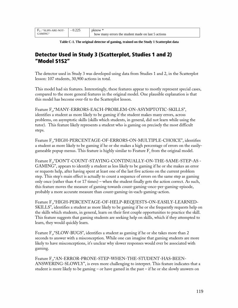
119

F3 : “SLIPS-ARE-NOT-GAMING”

- 0.225 pknow * how many errors the student made on last 5 actions

Table C-1. The original detector of gaming, trained on the Study 1 Scatterplot data

Detector Used in Study 3 (Scatterplot, Studies 1 and 2) “Model S1S2” The detector used in Study 3 was developed using data from Studies 1 and 2, in the Scatterplot lesson: 107 students, 30,900 actions in total. This model had six features. Interestingly, these features appear to mostly represent special cases, compared to the more general features in the original model. One plausible explanation is that this model has become over-fit to the Scatterplot lesson. Feature F

0,“MANY-ERRORS-EACH-PROBLEM-ON-ASYMPTOTIC-SKILLS”,

identifies a student as more likely to be gaming if the student makes many errors, across problems, on asymptotic skills (skills which students, in general, did not learn while using the tutor). This feature likely represents a student who is gaming on precisely the most difficult steps. Feature F

1,“HIGH-PERCENTAGE-OF-ERRORS-ON-MULTIPLE-CHOICE”, identifies

a student as more likely to be gaming if he or she makes a high percentage of errors on the easily-gameable popup menus. This feature is highly similar to Feature F

2 from the original model.

Feature F

2,“DON’T-COUNT-STAYING-CONTINUALLY-ON-THE-SAME-STEP-AS -

GAMING”, appears to identify a student as less likely to be gaming if he or she makes an error or requests help, after having spent at least one of the last five actions on the current problem step. This step’s main effect is actually to count a sequence of errors on the same step as gaming only once (rather than 4 or 17 times) – when the student finally gets the action correct. As such, this feature moves the measure of gaming towards count-gaming-once-per-gaming-episode, probably a more accurate measure than count-gaming-in-each-gaming-action. Feature F

3,“HIGH-PERCENTAGE-OF-HELP-REQUESTS-ON-EASILY-LEARNED-

SKILLS”, identifies a student as more likely to be gaming if he or she frequently requests help on the skills which students, in general, learn on their first couple opportunities to practice the skill. This feature suggests that gaming students are seeking help on skills, which if they attempted to learn, they would quickly learn. Feature F

4,“SLOW-BUGS”, identifies a student as gaming if he or she takes more than 2

seconds to answer with a misconception. While one can imagine that gaming students are more likely to have misconceptions, it’s unclear why slower responses would ever be associated with gaming. Feature F

5,“AN-ERROR-PRONE-STEP-WHEN-THE-STUDENT-HAS-BEEN-

ANSWERING-SLOWLY”, is even more challenging to interpret. This feature indicates that a student is more likely to be gaming – or have gamed in the past – if he or she slowly answers on

120

three steps and then reaches a step where he or she has a history of errors. Feature F4 is also very

weak, never reducing an action’s probability of gaming by more than 5-6%. These features are expressed formally in Table C-2.

Name Coefficient Feature F0 : “MANY-ERRORS-EACH-PROBLEM-ON-ASYMPTOTIC-SKILLS”

+ 0.2 number of errors the student has made on this problem step (across all problems), on asymptotic skills

F1: : “HIGH-PERCENTAGE-OF-ERRORS-ON-MULTIPLE-CHOICE”

+ 0.11875 percentage of errors, on multiple-choice popup menus

F2: “DON’T-COUNT-STAYING-CONTINUALLY-ON-THE-SAME-STEP-AS-GAMING”

-1.01 number of recent actions that have been on this problem step, when the student makes an error or requests help

F3: : “HIGH-PERCENTAGE-OF-HELP-REQUESTS-ON-EASILY-LEARNED-SKILLS”

+ 0.9 percentage of help requests, on skills most students learn quickly

F4 : “SLOW-BUGS” + 0.2875 time taken, when demonstrating a misconception

F5 : “AN-ERROR-PRONE-STEP-WHEN-THE-STUDENT-HAS-BEEN-ANSWERING-SLOWLY”

+ 0.0125 A high percentage of errors * time taken, in SD above (+) or below (-) the mean time for all students, on the last 3 problem steps

Table C-2. The detector of gaming used in Study 3 (trained on Scatterplot data from Studies 1 and 2)

Final Detector (Trained on All Available Data) “Model F” The final detector of gaming in this dissertation was developed using all of the data in this dissertation: 4 lessons, 473 students, 128,887 actions in total. This model had six features. One of the features is an exact duplicate of a feature in the original detector (F

0 in both models). Interestingly, four of the six features appear to primarily represent

behavior that is not gaming (as compared to one of four in the original detector). It is possible that the greater diversity of lessons trained on makes it more possible to identify special-case behaviors in a particular tutor lesson that might otherwise appear to be gaming. Feature F

0,“ERROR-NOW, MANY-ERRORS-EACH-PROBLEM”, identifies a student as

more likely to be gaming if the student has already made at least one error on this problem step within this problem, and has also made a large number of errors on this problem step in previous problems. It identifies a student as less likely to be gaming if the student has made a lot of errors on this problem step in the past, but now probably understands it (and has not yet gotten the step wrong in this problem). This was also the first feature in the original model, though it is more emphasized in this model.

Feature F

1,“ASKING-FOR-HELP-ON-WELL-KNOWN-STEPS”, identifies a student as

more likely to be gaming (or to have gamed in the past) if the student asks for help on skills that he or she has a high probability of knowing. In effect, this feature suggests that the student may have in the past obtained correct answers through lucky guesses, or through problem-specific strategies.

121

Feature F2,“POINT-PLOTTING-ERRORS-ARE-NOT-GAMING”,

identifies that students

may make a large number of errors on point plotting (in the scatterplot tutor) without the intention of gaming.

Feature F

3,“PAST-ERRORS-ON-A-NOW-KNOWN-SKILL-ARE-NOT-GAMING”,

identifies that if a student has a history of making many errors on a skill, but also now has a high probability of knowing the skill (obtained through getting right answers on the first try), they have probably stopped gaming (if they had been gaming). Feature F

3 is very weak, having a

maximum possible effect of reducing an action’s probability of gaming by 5.6% Feature F

4,“CLUSTERS-OF-HELP-REQUESTS-ARE-NOT-GAMING”,

identifies that a

cluster of help requests on different problem steps is not gaming. This feature is non-intuitive, but serves to refine Feature F

1, reducing the intensity of F

1’s effects when a student who has done

well on early problems finds some feature of a later problem enigmatic across several steps. Feature F

5,“SLOW-CORRECT-ANSWERS-ARE-NOT-GAMING”,

identifies –

unsurprisingly – that slow correct answers are not gaming.

These features are expressed formally in Table C-3.

Name Coefficient Feature F0 : “ERROR-NOW, MANY-ERRORS-EACH-PROBLEM”

-0.4375 pknow-direct * number of errors the student has made on this problem step (across all problems)

F1 : “ASKING-FOR-HELP-ON-WELL-KNOWN-STEPS”

+ 0.8625 pknow, when the student is requesting help

F2: : “POINT-PLOTTING-ERRORS-ARE-NOT-GAMING”

- 0.8625 number of errors in the last 5 steps, when the student is plotting a point

F3 : “PAST-ERRORS-ON-A-NOW-KNOWN-SKILL-NO-LONGER-MATTER”

- 0.05625 pknow * percentage of the time the student has gotten the current skill wrong, in the past

F4 : “CLUSTERS-OF-HELP-REQUESTS-ARE-NOT-GAMING”

-0.1375 number of help requests in the last 8 steps, when the student is requesting help

F5 : “SLOW-CORRECT-ANSWERS-ARE-NOT-GAMING”

-0.13125 time taken on the current step, for correct answers

Table C-3. The final detector of gaming, trained on all students and lessons

Detector Designed For More Exact Assessment of When Gaming Occurs “Model NPP” In order to analyze the tradeoff between detecting how much each student games and detecting when each student games, I trained a detector which does not use information from past problems when assessing whether an action is an instance of gaming. This detector was developed using all of the data in this dissertation: 4 lessons, 473 students, 128,887 actions in total. This model had seven features. As with the full model, several of the features appear to primarily represent behavior that is not gaming.

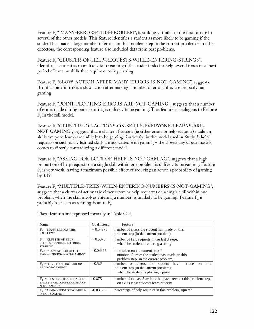
122

Feature F0,“ MANY-ERRORS-THIS-PROBLEM”, is strikingly similar to the first feature in

several of the other models. This feature identifies a student as more likely to be gaming if the student has made a large number of errors on this problem step in the current problem – in other detectors, the corresponding feature also included data from past problems. Feature F

1,“CLUSTER-OF-HELP-REQUESTS-WHILE-ENTERING-STRINGS”,

identifies a student as more likely to be gaming if the student asks for help several times in a short period of time on skills that require entering a string. Feature F

2,“SLOW-ACTION-AFTER-MANY-ERRORS-IS-NOT-GAMING”, suggests

that if a student makes a slow action after making a number of errors, they are probably not gaming. Feature F

3,“POINT-PLOTTING-ERRORS-ARE-NOT-GAMING”, suggests that a number

of errors made during point plotting is unlikely to be gaming. This feature is analogous to Feature F

2 in the full model.

Feature F

4,“CLUSTERS-OF-ACTIONS-ON-SKILLS-EVERYONE-LEARNS-ARE-

NOT-GAMING”, suggests that a cluster of actions (ie either errors or help requests) made on skills everyone learns are unlikely to be gaming. Curiously, in the model used in Study 3, help requests on such easily learned skills are associated with gaming – the closest any of our models comes to directly contradicting a different model. Feature F

5,“ASKING-FOR-LOTS-OF-HELP-IS-NOT-GAMING”, suggests that a high

proportion of help requests on a single skill within one problem is unlikely to be gaming. Feature F

5 is very weak, having a maximum possible effect of reducing an action’s probability of gaming

by 3.1% Feature F

6,“MULTIPLE-TRIES-WHEN-ENTERING-NUMBERS-IS-NOT-GAMING”,

suggests that a cluster of actions (ie either errors or help requests) on a single skill within one problem, when the skill involves entering a number, is unlikely to be gaming. Feature F

6 is

probably best seen as refining Feature F0.

These features are expressed formally in Table C-4.

Name Coefficient Feature F0 : “MANY-ERRORS-THIS-PROBLEM”

+ 0.54375 number of errors the student has made on this problem step (in the current problem)

F1 : “CLUSTER-OF-HELP-REQUESTS-WHILE-ENTERING-STRINGS”

+ 0.5375 number of help requests in the last 8 steps, when the student is entering a string

F2: : “SLOW-ACTION-AFTER-MANY-ERRORS-IS-NOT-GAMING”

- 0.04375 time taken on the current step * number of errors the student has made on this problem step (in the current problem)

F3 : “POINT-PLOTTING-ERRORS-ARE-NOT-GAMING”

- 0.525 number of errors the student has made on this problem step (in the current problem), when the student is plotting a point

F4 : “CLUSTERS-OF-ACTIONS-ON-SKILLS-EVERYONE-LEARNS-ARE-NOT-GAMING”

-0.875 number of the last 5 actions that have been on this problem step, on skills most students learn quickly

F5 : “ASKING-FOR-LOTS-OF-HELP-IS-NOT-GAMING”

-0.03125 percentage of help requests in this problem, squared

123

F6 : “MULTIPLE-TRIES-WHEN-ENTERING-NUMBERS-IS-NOT-GAMING”

-0.14375 number of the last 5 actions that have been on this problem step, when the student is entering a number

Table C-4. The detector of gaming, trained on all students and lessons, using no data from past problems

124