designing systems for dependability and predictability
TRANSCRIPT

Designing Systems for Dependability and Predictability
Richard West
Boston University
Boston, MA

Introduction: Existing OSes
� Today’s world of operating systems:� Desktop
� e.g., MS Vista, Mac OS X, Linux� Server
� e.g., Solaris, Linux� Embedded (Real-time, mobile etc)
� e.g., VxWorks, QNX, VRTX, Symbian, PalmOS…
� Revisiting an old idea: Virtualization� VM kernels and monitors
� e.g., VMware ESX Server, Xen
Virtualization – What’s the Big Deal?
� Virtualization is BIG!� Revisiting an idea from 1960s (e.g., IBM s/360)� New chips from Intel (VT/Vanderpool), AMD (Pacifica)
and others for CPU virtualization
� Good for server consolidation, disaster recovery, prototyping / sandboxing...
� BUT…� The VM kernel is the new OS� Is it really different from other OS kernels?
� e.g., micro-kernels

So Not Much New Then…
� What’s missing with today’s OSes?
(1) Semantic gap � between application needs and service provisions of
the system
(2) Time management � time is not a first-class resource
(3) Static system structure� Are you a “micro-kernel” guy or a member of the
church of monoliths?
Focus on Embedded Systems
� Currently numerous proprietary systems for RT/embedded computing� e.g., QNX, PSOS, LynxOS, VxWorks, VRTX� Many diverse hardware platforms
� ARM, x86, PowerPC, Hitachi SH, etc
� Focus on small footprints, fast context-switching, static priority/preemptive scheduling, priority inheritance/synchronization, limited / no VM, off-line profiling tools for WCET analysis

COTS / Open-Source Systems
� COTS hardware and open-source systems emerging� Eliminate costs of proprietary systems and custom
hardware� e.g., Linux use in embedded/RT settings
� BUT…� Problems as mentioned earlier:
� Semantic gap� Time management� Static structure

Bridging the `Semantic Gap’
� There is a `semantic gap’ between the needs of applications and services provided by the system
� Implementing functionality directly in application processes� Pros: service/resource isolation (e.g., memory protection)� Cons:
� Does not guarantee necessary responsiveness� Must leverage system abstractions in complex ways� Heavyweight scheduling, context-switching and IPC
overheads
Bridging the `Semantic Gap’ Cont.
� Other approaches:
� Special systems designed for extensibility
� e.g., SPIN, VINO, Exo-/µ-kernels (Aegis / L4), Palladium
� Semantics of new services restricted by those upon which they are built
� e.g., IPC costs → no timeliness / predictability guarantees on service invocation
� Single-address space approaches
� Do not focus on isolation of service extensions from core kernel (e.g., RTLinux, RTAI) or predictability (e.g., Singularity)

Time Management
� Inherent unpredictability in existing systems� Arbitrary orderings of accesses to shared resources
requires synchronization� Possibly unbounded blocking delays� Basic primitives provided by system but may be
incorrectly used by programs! � Deadlocks & races may still occur
� Interrupts, paging activity, unaccounted time in system services (scheduling / dispatching / IPC)
� Crosstalk b/w different threads due to resource sharing (e.g., cache, TLB impacts)

Time Management (cont.)
� Time is not a first-class resource� APIs don’t allow specification of time bounds on service
requests (e.g., read / write I/O requests)� Not even implicit specification based on urgency /
importance of a task
� Scheduling / resource mgmt policies are not explicitly temporal

Static System Structure
� Monolithic systems (e.g., Linux) are inflexible to changes in structure and services they support� Do support kernel modules (mostly for device drivers),
but…� Not easily customizable with app-specific services� No support for extensions to override system-wide
service policies
� While micro-kernels support extensibility, the organization of system services is statically-defined� system designer typically determines which services are
available and how they are isolated� Is this organization suitable for all applications?

Static System Structure (cont.)
� Resource contention and changes in availability affect predictability of service requests
� IPC costs, scheduling / dispatching / context-switching / TLB flushing, cache usage patterns, etc � affect time to complete service requests
� A static organization of services cannot adapt to dynamic variations in resource usage and service invocation patterns

Example: App-Specific System Structure
Planet surface Earth
Data acquisition
Communication
Motor / sensor control
RobotExploration
Service Characteristics
� Different timing requirements / criticalities in terms of late or missed processing
� e.g., can miss some data (image) acquisition but sensor & motor control operations are more critical
� Safety / dependability trade-offs
� Scheduling functionality isolated from services to collect, process & communicate data
� Communication functionality must be maintained in case of need for remote reboot or changes to mission objectives
� Data gathering service not so safety critical
� e.g., direct access to a buffer (and overruns) not catastrophic, as long as base services remain functional
� Design systems around flexibility in system structure

Example: Intelligent Home Network
� www.epa.gov/ne/pr/2004/jan/040110.html� Study suggested that by replacing 5 most used light-
bulbs w/ energy efficient bulbs in every US household could reduce electricity usage by 800 billion KWh per year� Equivalent to $60/yr per homeowner or output from 21
power plants per year� Would reduce one trillion pounds of greenhouse gases
that cause global warming
� Allow homeowners to control various appliances according to desired energy plan

Example: Intelligent Home (cont.)
� Homeowner service may query service providers billing service BUT should not be able to change a billing policy
� Gas and Electric Co. may share billing / appliance monitoring services if part of the same parent company
� Appliance control & usage accounting needs to be predictable → avoid customer mis-charges for appliance usage
Base services (Device mgmt)
Electric Co.Accnting / Billing Service
Gas Co.Accnting / Billing Service
HomeownerConfigurable Energy Plan

Case Studies
(1) Improving time management (predictability) in existing systems� e.g., Process-aware interrupt scheduling and accounting
in Linux
(2) Mutable Protection Domains (MPDs)� Dynamically reorganize system component services to
meet safety (isolation) and predictability (resource) requirements

Process-Aware Interrupt Scheduling & Accounting
(1) Improving Time Management (Predictability) in Existing Systems

Commodity OSes for Real-Time
� Many variants based on systems such as Linux:� Linux/RK, QLinux, RED-Linux, RTAI, KURT Linux, and
RT Linux� e.g., RTLinux Free provides predictable execution of
kernel-level real-time tasks� Bounds are enforced on interrupt processing
overheads by deferring non-RT tasks when RT tasks require service
� NOTE: Many commodity systems suffer unpredictability (unbounded delays) due to interrupt-disabling, e.g., in critical sections of poorly-written device drivers

The Problem of Interrupts
� Asynchronous events e.g., from hardware completing I/O requests and timer interrupts…
� Affect process/thread scheduling decisions
� Typically invoke interrupt handlers at priorities above those of processes/threads
� i.e., interrupt scheduling disparate from process/thread scheduling
� Time spent handling interrupts impacts the timeliness of RT tasks and their ability to meet deadlines
� Overhead of handling an interrupt is charged to the process that is running when the interrupt occurs
� Not necessarily the process associated (if any) with the interrupt

Goals
� How to properly account for interrupt processing and correctly charge CPU time overheads to correct process, where possible
� How to schedule deferrable interrupt handling so that predictable task execution is guaranteed

Interrupt Handling
� Interrupt service routines are often split into “top” and “bottom” halves� Idea is to avoid lengthy periods of time in “interrupt
context”� Top half executed at time of interrupt but bottom half may
be deferred (e.g., to a schedulable thread)

Process-Independent Interrupt Service
� Traditional approach:
� I/O service request via kernel
� OS sends request to device via driver code;
� Hardware device responds w/ an interrupt, handled by a “top half”
� Deferrable “bottom half” completes service for prior interrupt and wakes waiting process(es) – Usually runs w/ interrupts enabled
� A woken process can then be scheduled to resume after blocking I/O request
Processes
OS
Interrupt handler
Top Halves
Bottom Halves
P1 P2 P3 P4
Hardware
interrupts
1
2
3
4
1
2
3
4
Example: Linux
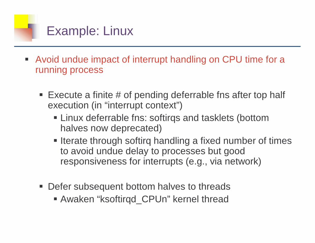
� Avoid undue impact of interrupt handling on CPU time for a running process
� Execute a finite # of pending deferrable fns after top half execution (in “interrupt context”)� Linux deferrable fns: softirqs and tasklets (bottom
halves now deprecated)� Iterate through softirq handling a fixed number of times
to avoid undue delay to processes but good responsiveness for interrupts (e.g., via network)
� Defer subsequent bottom halves to threads� Awaken “ksoftirqd_CPUn” kernel thread

Linux Problems
� A real-time or high-priority blocked process waiting on I/O may be unduly delayed by a deferred bottom half� Mismatch between bottom half priority and process
� Interrupt handling takes place in context of an arbitrary process� May lead to incorrect CPU time accounting
� Why not schedule bottom halves in accordance with priorities of processes affected by their execution?
� For fairness and predictability: charge CPU time of interrupt handling to affected process(es), where possible
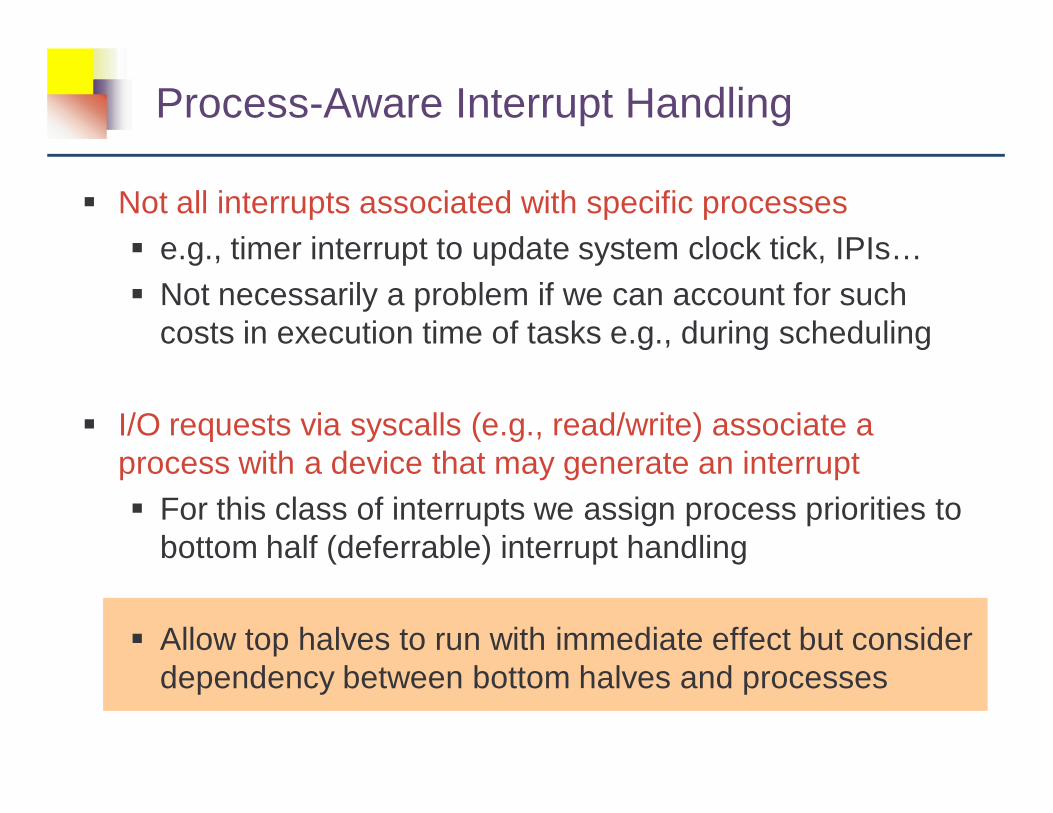
Process-Aware Interrupt Handling
� Not all interrupts associated with specific processes� e.g., timer interrupt to update system clock tick, IPIs…� Not necessarily a problem if we can account for such
costs in execution time of tasks e.g., during scheduling
� I/O requests via syscalls (e.g., read/write) associate a process with a device that may generate an interrupt� For this class of interrupts we assign process priorities to
bottom half (deferrable) interrupt handling
� Allow top halves to run with immediate effect but consider dependency between bottom halves and processes

Bottom Half Scheduling / Accounting
� Modify Linux kernel to include interrupt accounting
� TSC measurements on bottom halves
� Determine target process for interrupt processing and update system time accordingly
� BH/interrupt scheduler immediately between do_irq() and do_softirq()
� Predict target process associated with interrupt and set BH priority accordingly
BH schedulerOS
Interrupt handler
Top Halves
Bottom Halves
BH accounter

Interrupt Accounting Algorithm
� Measure the average execution time of a bottom half (BH) across multiple BH executions� On x86 use rdtsc since time granularity typically < 1 clock
tick� Measure total interrupts processed and # processed for
each process in 1 clock tick� Adjust system CPU time for processes due to mischarged
interrupt costs
� For simplicity, focus on interrupts for one device type (e.g., NIC) but idea applies to all I/O devices

System CPU Time Compensation (1/2)
� N(t) - integer # interrupts whose total BH execution time = 1 clock tick (or jiffy)� Actually use an Exponentially-Weighted Moving Avg for
N(t), N’(t)� N’(t) = (1-γ)N’(t-1) + γ N(t) | 0 < γ < 1
� m(t) - # interrupts processed in last clock tick� xk(t) - # unaccounted interrupts for process Pk
� Let Pi(t) be active at time t� m(t) – xi(t) (if +ve) is # interrupts overcharged to Pi
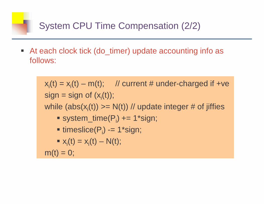
System CPU Time Compensation (2/2)
� At each clock tick (do_timer) update accounting info as follows:
xi(t) = xi(t) – m(t); // current # under-charged if +vesign = sign of (xi(t));while (abs(xi(t)) >= N(t)) // update integer # of jiffies
� system_time(Pi) += 1*sign;� timeslice(Pi) -= 1*sign;� xi(t) = xi(t) – N(t);
m(t) = 0;

Example: System CPU Time Compensation
t0 1 2 3 4 5 6 7 8P1
P1 P3 P4
P1
P2 P1 P3
I1 I2 I1 I3 I2 I3 I1 I1 I4 I3 I2I1 I1 I4 I3 I2 I1 I1 I3I3
P2
x1(1): -3 + 2 = -1, x2(2): -1 + 1= 0, x3(3): -2 + 2 = 0, x4(4) : -3 + 1 =-2, x4(5): -2 + -4+ 0= -6, x2(6): 0 + -2 + 2 = 0,x1(7): -1 + -2+ 4= 1, x3(8): 0 + -3 + 4 = 1,

Interrupt Scheduling Algorithm
� (1) Find candidates associated with interrupt on device, D� In top half can determine D� A blocked process waiting on D may be associated with
the interrupt� We require I/O requests to register process ID and
priorities with corresponding device� (2) Predicting process associated with interrupt on D
� At end of top half select highest priority (ρmax(D)) from processes waiting on D
� Use a heap structure for waiting processes� (3) Compare priority of BH with running process
� If (ρmax(D) = ρBH) > ρcurrent run BH else process
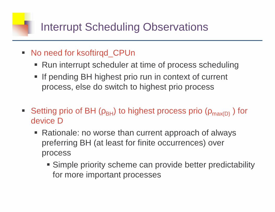
Interrupt Scheduling Observations
� No need for ksoftirqd_CPUn� Run interrupt scheduler at time of process scheduling� If pending BH highest prio run in context of current
process, else do switch to highest prio process
� Setting prio of BH (ρBH) to highest process prio (ρmax(D) ) for device D� Rationale: no worse than current approach of always
preferring BH (at least for finite occurrences) over process� Simple priority scheme can provide better predictability
for more important processes
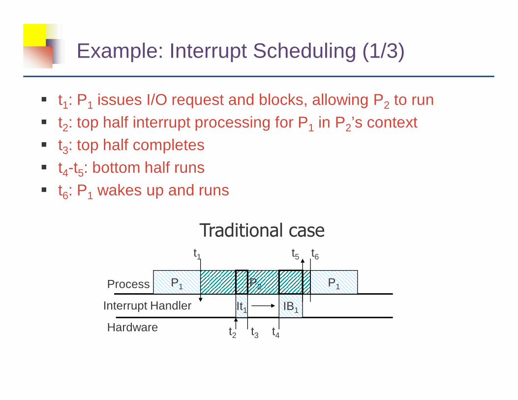
Example: Interrupt Scheduling (1/3)
� t1: P1 issues I/O request and blocks, allowing P2 to run� t2: top half interrupt processing for P1 in P2’s context� t3: top half completes� t4-t5: bottom half runs� t6: P1 wakes up and runs
t1 t6
Interrupt Handler
Process
Hardware
P1 P2
It1 IB1
P1
t2 t3 t4
t5
Traditional case
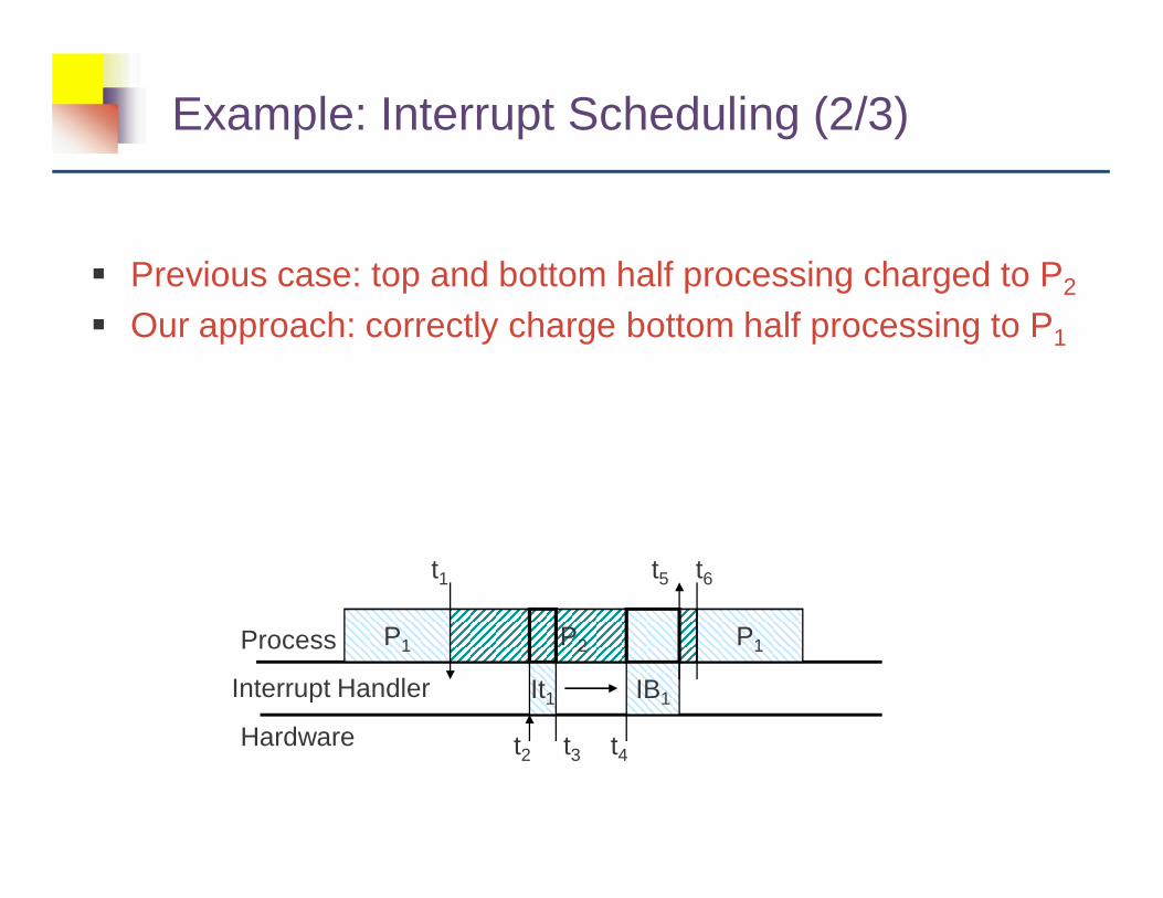
Example: Interrupt Scheduling (2/3)
� Previous case: top and bottom half processing charged to P2
� Our approach: correctly charge bottom half processing to P1
Interrupt Handler
Process
Hardware
P1 P2
It1 IB1
P1
t2 t3 t4
t1 t6t5

Example: Interrupt Scheduling (3/3)
� If P2 is higher priority than P1, let P2 finish and defer the BH for P1
Interrupt Handler
Process
Hardware
P1
It1 IB1
P1
t1
t2 t3 t4
t5
P2

System Implementation
� Implemented scheduling & accounting framework on top of existing Linux bottom half (specifically, softirq) mechanism
� Focus on network packet reception (NET_RX_SOFTIRQ)� Read TSC for each net_rx_action call as part of softirq� Determine # pkts received in one clock tick� udp_rcv() identifies proper socket/process for arriving pkt(s)
� Modify account_system_time() to compensate processes
� Interrupt scheduling code implemented in do_softirq()� Before call to softirq handler (e.g., net_rx_action())
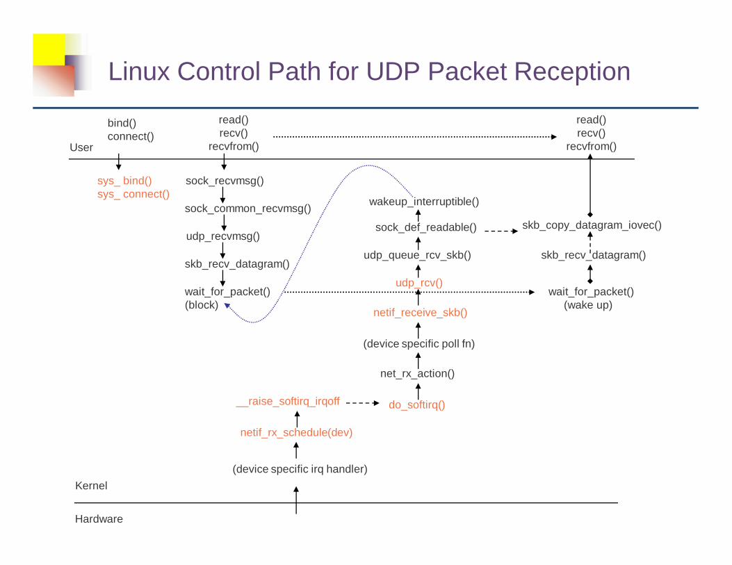
Linux Control Path for UDP Packet Reception
bind()connect()
sys_ bind()sys_ connect()
read()recv()
recvfrom()
sock_recvmsg()
sock_common_recvmsg()
udp_recvmsg()
skb_recv_datagram()
wait_for_packet()(block)
(device specific irq handler)
netif_rx_schedule(dev)
__raise_softirq_irqoff
net_rx_action()
(device specific poll fn)
netif_receive_skb()
do_softirq()
udp_rcv()
udp_queue_rcv_skb()
sock_def_readable()
wakeup_interruptible()
wait_for_packet()(wake up)
skb_copy_datagram_iovec()
read()recv()
recvfrom()User
Kernel
Hardware
skb_recv_datagram()

Experiments
� UDP server receives pkts on designated port� CPU-bound process also active on server to observe
effect of interrupt handling due to pkt processing� UDP client sends pkts to server at adjustable rates
� Machines have 2.4GHz Pentium IV uniprocessors and 1.2GB RAM each
� Gigabit Ethernet connectivity� Linux 2.6.14 with 100Hz timer resolution
� Compare base 2.6.14 kernel w/ our patched kernel running accounting (Linux-IA) and scheduling (Linux-ISA) code
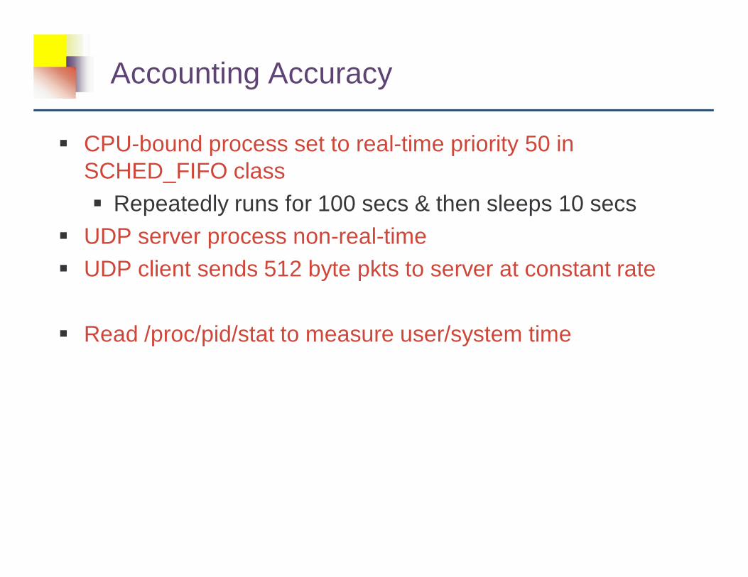
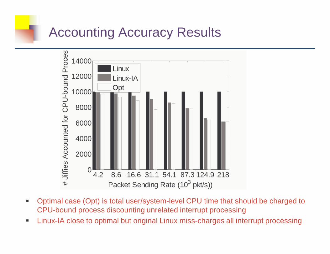
Accounting Accuracy
� CPU-bound process set to real-time priority 50 in SCHED_FIFO class� Repeatedly runs for 100 secs & then sleeps 10 secs
� UDP server process non-real-time� UDP client sends 512 byte pkts to server at constant rate
� Read /proc/pid/stat to measure user/system time
Accounting Accuracy Results
4.2 8.6 16.6 31.1 54.1 87.3 124.9 2180
2000
4000
6000
8000
10000
12000
14000
Packet Sending Rate (103 pkt/s))# Ji
ffies
Acc
ount
ed fo
r C
PU
-bou
nd P
roce
ss
LinuxLinux-IAOpt
� Optimal case (Opt) is total user/system-level CPU time that should be charged to CPU-bound process discounting unrelated interrupt processing
� Linux-IA close to optimal but original Linux miss-charges all interrupt processing
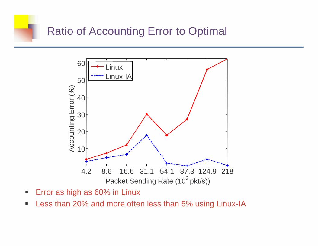
Ratio of Accounting Error to Optimal
� Error as high as 60% in Linux
� Less than 20% and more often less than 5% using Linux-IA
4.2 8.6 16.6 31.1 54.1 87.3 124.9 218
10
20
30
40
50
60
Packet Sending Rate (103 pkt/s))
Acc
ount
ing
Err
or (
%)
LinuxLinux-IA

Absolute Compensated Time
4.2 8.6 16.6 31.1 54.1 87.3 124.9 2180
1000
2000
3000
4000
Packet Sending Rate (103 pkt/s))
Abs
(Com
pens
ated
Tim
e) (
jiffie
s)
CPU-boundUDP-Server(a)UDP-Server(b)
� UDP-Server(a) – charged time for interrupts over 100s of each 110s period of CPU bound process
� UDP-Server(b) – charged time over full 110s period� CPU-bound – system service time deducted from CPU-bound process

Bottom Half Scheduling Effects
4.2 8.6 16.6 31.1 54.1 87.3 124.9 2180
2000
4000
6000
8000
10000
12000
Packet Sending Rate (103 pkt/s))# Ji
ffies
Con
sum
ed b
y C
PU
-bou
nd P
roce
ss
LinuxLinux-ISA
� Linux – CPU-bound process affected by interrupts
� Linux-ISA – defer bottom-half interrupt processing until (higher priority) real-time CPU-bound process sleeps

Time Consumed by Interrupts (every 110s)
4.2 8.6 16.6 31.1 54.1 87.3 124.9 2180
1000
2000
3000
4000
5000
Packet Sending Rate (103 pkt/s))
# Ji
ffies
Con
sum
ed b
y In
terr
upts
LinuxLinux-ISA
� Time consumed by CPU-server every 110s handling interrupts
� Linux-ISA – bottom half handling deferred to interval [100-110s]
� Linux – bottom half processing not deferred

UDP-Server Packet Reception Rate
4.2 8.6 16.6 31.1 54.1 87.3 124.9 2180
2
4
6
8
10
12
Packet Sending Rate (103 pkt/s))
% P
kts
Rec
eive
d by
UD
P-s
erve
r
LinuxLinux-ISA
Bursty Packet Transmission Experiments
� UDP-client sends bursts of pkts w/ avg geometric sizes of 5000 pkts� Different avg exponential burst inter-arrival times
� CPU-bound process is periodic w/ C=0.95s and T=1.0s� Runs for 100s as before
� Deadline at end of each 1s period

Deadline Miss Rate
� Linux-ISA – no missed deadlines for CPU-bound process
� Bottom half interrupt handling deferred until CPU-bound process completes each period
4.2 8.6 16.6 31.1 54.1 87.3 124.9 2180
20
40
60
80
100
Packet Sending Rate (103 pkt/s))
Dea
dlin
e M
iss
Rat
e (%
)LinuxLinux-ISA
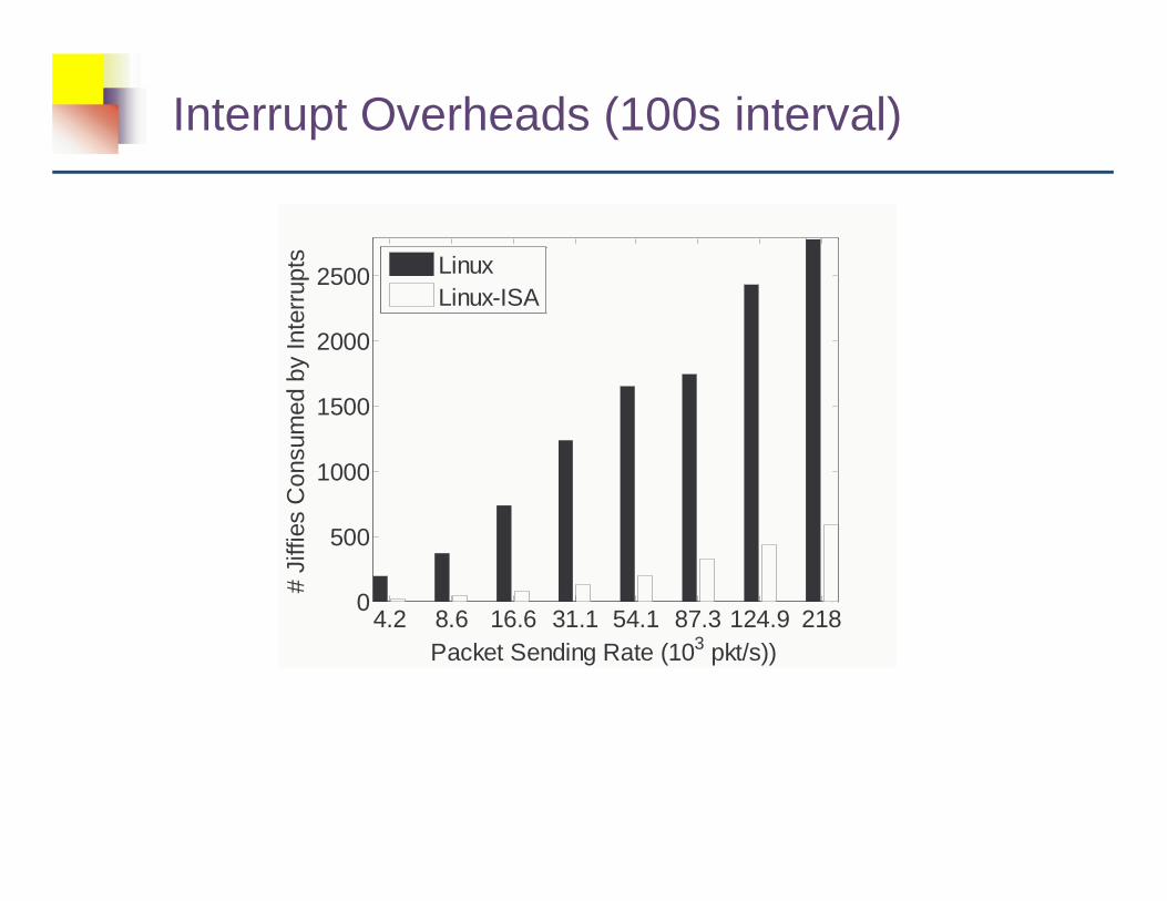
Interrupt Overheads (100s interval)
4.2 8.6 16.6 31.1 54.1 87.3 124.9 2180
500
1000
1500
2000
2500
Packet Sending Rate (103 pkt/s))
# Ji
ffies
Con
sum
ed b
y In
terr
upts
LinuxLinux-ISA

Performance of UDP-server
4.2 8.6 16.6 31.1 54.1 87.3 124.9 2180
2
4
6
8
10
12
Packet Sending Rate (103 pkt/s))
% P
kts
Rec
eive
d by
UD
P-s
erve
r
LinuxLinux-ISA
� CPU-bound process cannot finish executing in 1s period when interrupt overheads are high
� Always competes for CPU cycles, starving lower priority UDP-server
� Linux-ISA guarantees “slack” time usage for UDP-server
Conclusions and Future Work
� Explore dependency between processes and interrupts� Focus on bottom half scheduling and accounting
� Compensate processes for time spent in bottom halves� Charge correct processes benefiting from interrupts
� Unify the scheduling of bottom half interrupt handlers w/ processes � Improve predictability of real-time tasks while avoiding
undue interrupt-handling overheads� Consequently, benefit non-real-time tasks also!
� Future? Better predictors of process(es) associated w/ interrupts for scheduling purposes
� Interrupt management on multi-processors/cores

Towards a Component-based System for Dependable and Predictable Computing
(2) Mutable Protection Domains
Complexity of Embedded Systems
� Traditionally simpler software stack� limited functionality and complexity� focused application domain
� Soon cellphones will have 10s of millions of lines of code� downloadable content (with real-time constraints)
� Trend towards increasing complexity of embedded systems

Consequences of Complexity
� Run-time interactions are difficult to predict and can cause faults� accessing/modifying memory regions unintentionally� corruption to data-structures� deadlocks/livelocks� race-conditions� . . .
� Faults can cause violations in correctness and predictability

Designing for Dependability & Predictability
� Given increasing complexity, system design must anticipate faults
� Memory fault isolation: limit scope of adverse side-effects of errant software� identify and restart smallest possible section of the
system� recover from faults with minimal impact on system goals� employ software/hardware techniques
Preserve system reliability and predictability in spite of misbehaving and/or faulty software

Trade-offs in Isolation Granularity
Stack
Protection Domains
Increased Isolation Reduced Communication Cost
Components
Process Isolation User-kernel Isolation Library Isolation
Thread
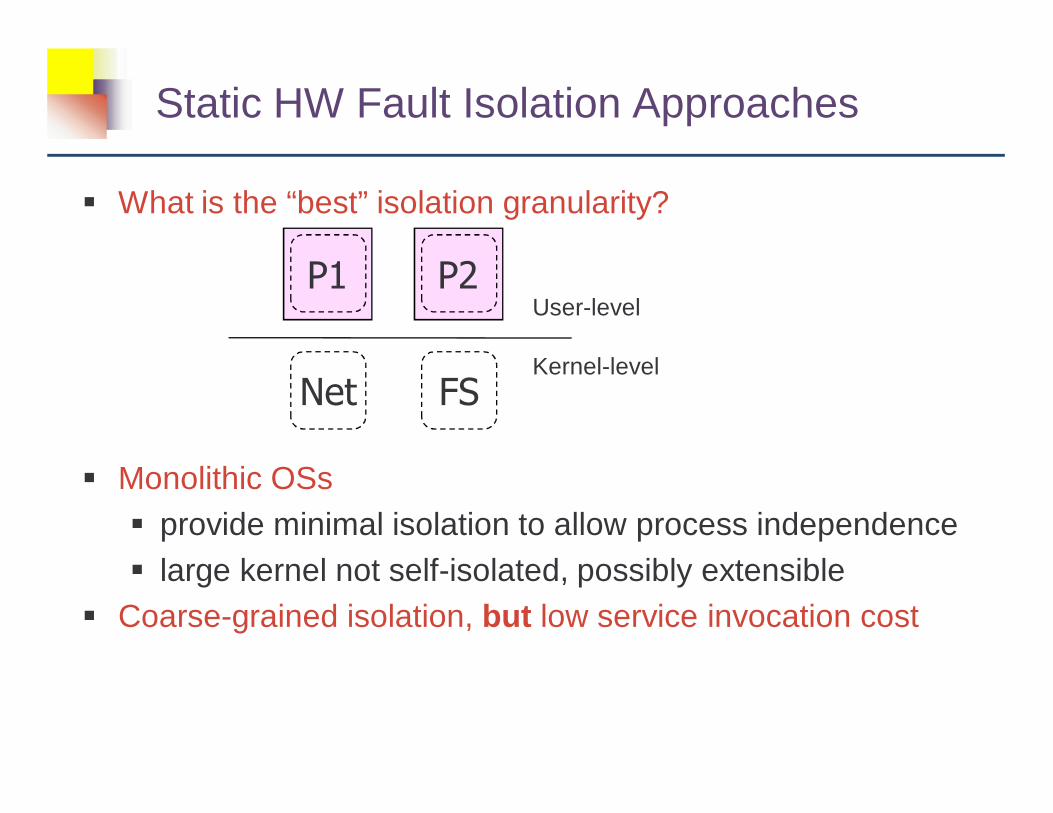
Static HW Fault Isolation Approaches
� What is the “best” isolation granularity?
� Monolithic OSs� provide minimal isolation to allow process independence� large kernel not self-isolated, possibly extensible
� Coarse-grained isolation, but low service invocation cost
P1 P2
Net FS
User-level
Kernel-level

Static HW Fault Isolation Approaches (II)
� What is the “best” isolation granularity?
� -kernels� segregate system services out of the kernel, interact w/
Inter-Process Communication (IPC)� finer-grained isolation
� IPC overhead limits isolation granularity� Finer-grained fault isolation, but increased service
invocation cost
P1 P2 User-level
Kernel-level
Net FS
IPC

Mutable Protection Domains (MPD)
Goal: configure system to have finest grained fault isolation while still meeting application deadlines
� Mutable Protection Domains (MPDs)� dynamically place protection domains between
components in response to� communication overheads due to isolation� application deadlines being satisfied
� application close to missing deadlines� lessen isolation between components
� laxity in application deadlines� increase isolation between components
Mutable Protection Domains (MPD) (II)
� Mutable Protection Domains appropriate for soft real-time systems
� Protection domains can be made immutable where appropriate

Setup and Assumptions
� System is a collection of components� Arranged into a directed acyclic graph (DAG)
� nodes = components themselves� edges = communication between them, indicative of
control flow
� Isolation over an edge can be configured to be one of the three isolation levels
Stack
Protection Domains
Thread
Components

Isolation cost and benefit
� Isolation between components causes a performance penalty due to:(1) processing cost of a single invocation between those
components(2) the frequency of invocations between those components⇒ cost of each isolation level/edge
� Isolation levels affect dependability� stronger isolation ⇒ higher dependability
� Isolation between specific components more important� debugging, testing, unreliable components, . . .⇒ benefit of each isolation levels/edge
Problem Definition
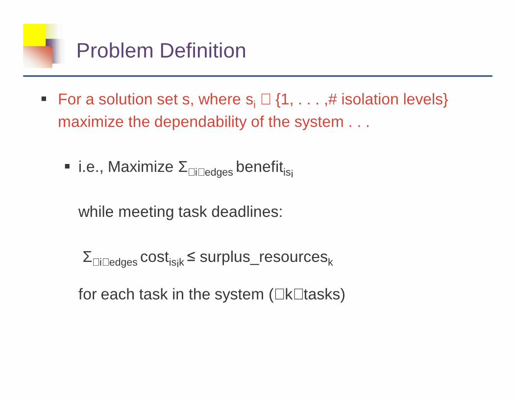
� For a solution set s, where si ∈ {1, . . . ,# isolation levels}maximize the dependability of the system . . .
� i.e., Maximize Σ∀i∈edges benefitisi
while meeting task deadlines:
Σ∀i∈edges costisik surplus_resourcesk
for each task in the system (∀k∈tasks)
Multi-Dimensional, Multiple-Choice Knapsack
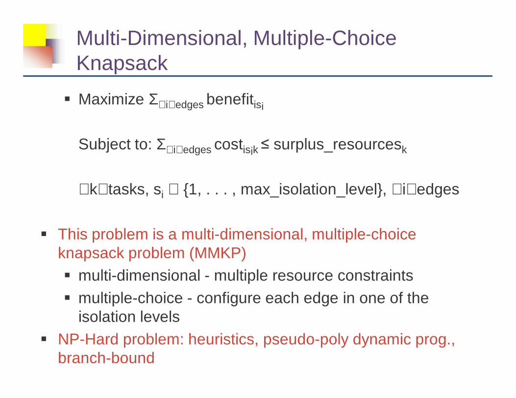
� Maximize Σ∀i∈edges benefitisi
Subject to: Σ∀i∈edges costisik surplus_resourcesk
∀k∈tasks, si ∈ {1, . . . , max_isolation_level}, ∀i∈edges
� This problem is a multi-dimensional, multiple-choice knapsack problem (MMKP)� multi-dimensional - multiple resource constraints� multiple-choice - configure each edge in one of the
isolation levels� NP-Hard problem: heuristics, pseudo-poly dynamic prog.,
branch-bound

One-Dimensional Knapsack Problem
� Effective and inexpensive greedy solutions to one-dimensional knapsack problem exist
� sort isolation levels/edges based on benefit density� ratio of benefit to cost
� increase isolation by including isolation levels/edges from head until resources are expended
. . . but we have multiple dimensions of cost
Solutions - Reducing Resource Dimensions
� Compute an aggregate cost for each edge� single value representing a combination of the costs for
all tasks for an edge: ∀k, costisik → agg_costisi
� some tasks very resource constrained, some aren’t� intelligently weight costs for task k to compute aggregate
cost

Solutions - HEU
� (1) compute aggregate cost for each isolation level/edge� (2) include isolation level/edge with best benefit density in
solution configuration� (3) goto 1 until resources expended
� Fine-grained refinement of aggregate cost� Re-compute once every time an isolation level/edge is
added to the current solution configuration
Solutions - coarse and oneshotRefinement
� (1) compute aggregate cost for each isolation level/edge
� (2) sort by benefit density
� (3) include isolation level/edge from head
� (4) goto 3, until resources expended
� (5) re-compute aggregate costs based on resource surpluses with solution configuration
� (6) goto 2 N times and return highest benefit configuration
� N > 1: coarse-grained refinement
� Re-compute once per total configuration found
� Execution time linearly increases with N
� N = 1: oneshot
� Very quick
� No aggregate cost refinement
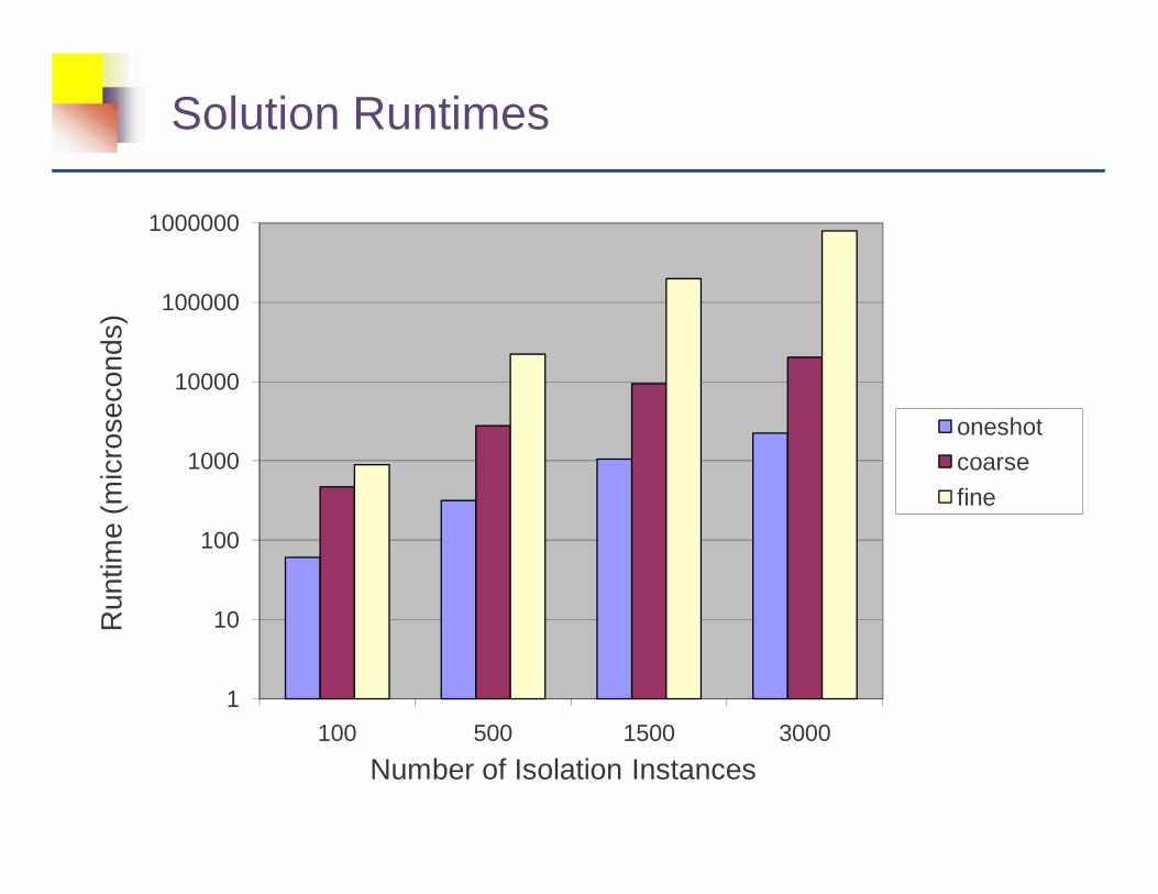
Solution Runtimes
1
10
100
1000
10000
100000
1000000
100 500 1500 3000
Run
time
(mic
rose
cond
s)
Number of Isolation Instances
oneshot
coarse
fine

System Dynamics
� System is dynamic� Changing communication costs over edges as threads
alter execution paths between components� Changing resource availabilities as threads vary intra-
component execution time� Per-invocation overheads vary
� Different cache working sets, invocation argument size, etc, . . .
� System must refine the system isolation configuration as these variables change

Solutions over time
� System dynamics require re-computation of system configuration� (1) disregard current system state, re-compute entirely
new system configuration� Traditional knapsack (MMKP) approach: ks
� (2) solve for the next system configuration starting from the current system configuration� Successive State Heuristic (ssh)
� modifies coarse and oneshot to start from the current system configuration
� aim to reduce isolation changes to existing configuration

Experimental Simulations
� Simulate a system with� widely varying resource surplus for 3 tasks� changing communication costs� 200 edges, 3 isolation levels� Edge benefits uniform & randomly chosen from [0,255]
for highest isolation level� Linear decrease to 0 for corresponding edge’s lowest
isolation level
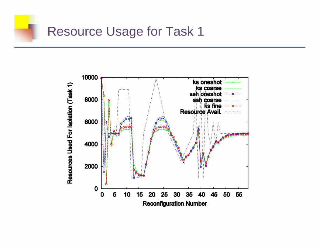
Resource Usage for Task 1

System Isolation-Derived Benefit
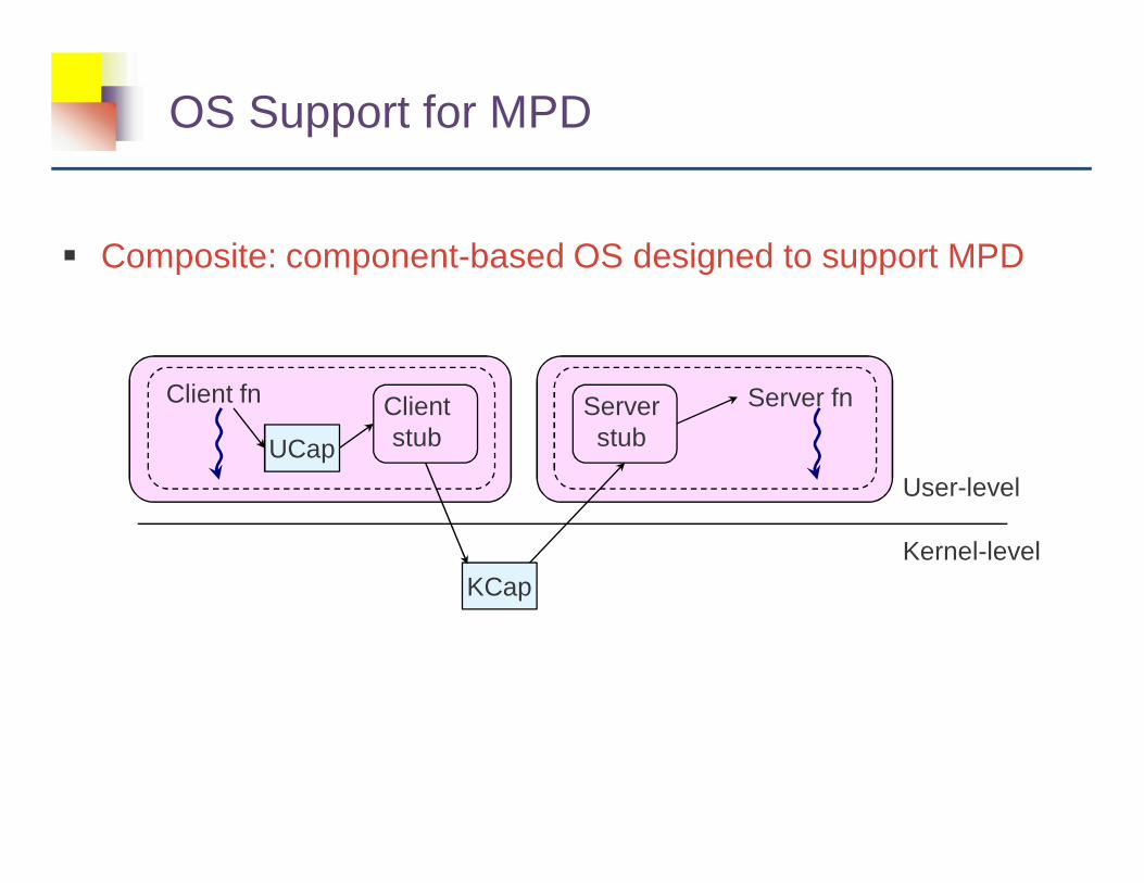
OS Support for MPD
� Composite: component-based OS designed to support MPD
User-level
Kernel-level
UCap
Client fn Clientstub
Serverstub
Server fn
KCap

OS Support for MPD (II)
� Composite: component-based OS designed to support MPD
User-level
Kernel-levelKCap
UCap
Client fn Clientstub
Serverstub
Server fn

OS Support for MPD (III)
� Switching between the two isolation levels requires changing UCap, KCap, and protection domains
� Prototype running on x86 Pentium IV @ 2.4 Ghz� Invocation via kernel - 1510 cycles (0.63 secs)� Direct invocation - 55 cycles (0.023 secs)
Conclusions
� Solution to MMKP based on lightweight successive refinement given dynamic changes in system behavior� possibly useful in e.g. QRAM
� Mutable Protection Domains� dynamically reconfigure protection domains to maximize
fault isolation while meeting application deadlines� makes the performance/predictability versus fault
isolation tradeoff explicit