designing the dynamic response of organic rankine cycle
TRANSCRIPT

This document is downloaded from DR‑NTU (https://dr.ntu.edu.sg)Nanyang Technological University, Singapore.
Designing the dynamic response of OrganicRankine Cycle evaporators in waste heat recoveryapplications
Jiménez‑Arreola, Manuel
2019
Jiménez‑Arreola, M. (2020). Designing the dynamic response of Organic Rankine Cycleevaporators in waste heat recovery applications. Doctoral thesis, Nanyang TechnologicalUniversity, Singapore.
https://hdl.handle.net/10356/140132
https://doi.org/10.32657/10356/140132
This work is licensed under a Creative Commons Attribution‑NonCommercial 4.0International License (CC BY‑NC 4.0).
Downloaded on 18 Oct 2021 22:08:34 SGT

DESIGNING THE DYNAMIC RESPONSE OF ORGANIC
RANKINE CYCLE EVAPORATORS IN WASTE HEAT
RECOVERY APPLICATIONS
MANUEL JIMÉNEZ ARREOLA
Interdisciplinary Graduate School
Energy Research Institute @ NTU
2019


DESIGNING THE DYNAMIC RESPONSE OF ORGANIC
RANKINE CYCLE EVAPORATORS IN WASTE HEAT
RECOVERY APPLICATIONS
MANUEL JIMÉNEZ ARREOLA
INTERDISCIPLINARY GRADUATE SCHOOL
A thesis submitted to the Nanyang Technological University in
partial fulfilment of the requirement for the degree of Doctor of
Philosophy
2019


Statement of Originality
I hereby certify that the work embodied in this thesis is the result of original research, is
free of plagiarised materials, and has not been submitted for a higher degree to any other
University or Institution.
02 August 2019
. . . . . . . . . . . . . . . . . . . . . . . . . . . . . . . . . . . . . . . . . . . .
Date Manuel Jiménez Arreola


Supervisor Declaration Statement
I have reviewed the content and presentation style of this thesis and declare it is free of
plagiarism and of sufficient grammatical clarity to be examined. To the best of my
knowledge, the research and writing are those of the candidate except as acknowledged in
the Author Attribution Statement. I confirm that the investigations were conducted in
accord with the ethics policies and integrity standards of Nanyang Technological
University and that the research data are presented honestly and without prejudice.
02 August 2019
. . . . . . . . . . . . . . . . . . . . . . . . . . . . . . . . . . . . . . . . . . . .
Date Asst. Prof. Alessandro Romagnoli


Authorship Attribution Statement
This thesis contains material from 4 papers published in the following peer-reviewed
journals and conference proceeding where I was the first author.
Chapter 2 is published partially as M. Jiménez-Arreola, R. Pili, F. Dal Magro, C. Wieland,
S. Rajoo and A. Romagnoli. Thermal power fluctuations in waste heat to power systems:
an overview on the challenges and current solutions. Applied Thermal Engineering 134,
576–584 (2018). DOI: 10.1016/j.applthermaleng.2018.02.033.
The contributions of the co-authors are as follows:
• I prepared the manuscript drafts. The manuscript was revised by Prof. Alessandro
Romagnoli, Dr. Christoph Wieland and Prof. Srithar Rajoo
• I compounded the literature review, performed the technical assessments, designed
the sections layout and prepared and formatted all figures.
• Mr. Roberto Pili provided the methods and calculations of the economics
considerations section.
• Dr. Fabio Dal Magro provided guidance on the technical assessment.
Chapter 4 is published partially as M. Jiménez-Arreola, C. Wieland and A. Romagnoli.
Response time characterization of Organic Rankine Cycle evaporators for dynamic regime
analysis with fluctuating load. Energy Procedia 129, 427–434 (2017). DOI:
10.1016/j.egypro.2017.09.131.
The contributions of the co-authors are as follows:
• I wrote the drafts of the manuscript. The manuscript was revised by Prof.
Alessandro Romagnoli and Dr. Christoph Wieland
• I performed all the dynamic simulations, built the response time maps and provided
the discussion and interpretation of results.
• Dr. Christoph Wieland and Alessandro Romagnoli assisted with ideas for the
development of the response time maps.

Chapter 5 is published as M. Jiménez-Arreola, R. Pili, C. Wieland and A. Romagnoli.
Analysis and comparison of dynamic behavior of heat exchangers for direct evaporation in
ORC waste heat recovery applications from fluctuating sources. Applied Energy 216, 724-
740 (2018). DOI: 10.1016/j.apenergy.2018.01.085.
The contributions of the co-authors are as follows:
• I wrote the drafts of the manuscript. The manuscript was revised by Prof.
Alessandro Romagnoli, Dr. Christoph Wieland and Mr. Roberto Pili
• I performed all the dynamic simulations, built the response time maps, performed
the application case study and provided the discussion and interpretation of results.
• Mr. Roberto Pili assisted on the interpretation of the results.
• Dr. Christoph Wieland and Alessandro Romagnoli assisted with ideas for the
development of the methodology
Chapter 6 is published as M. Jiménez-Arreola, C. Wieland and A. Romagnoli. Direct vs
indirect evaporation in Organic Rankine Cycle (ORC) systems: A comparison of the
dynamic behavior for waste heat recovery of engine exhaust. Applied Energy 242, 439-452
(2018). DOI: 10.1016/j.apenergy.2019.03.011
The contributions of the co-authors are as follows:
• I wrote the drafts of the manuscript. The manuscript was revised by Prof.
Alessandro Romagnoli and Dr. Christoph Wieland
• I performed all the dynamic simulations, built the response time maps, performed
the application case study, developed the concepts of the amplitude ratio and
provided the discussion and interpretation of results.
• Dr. Christoph Wieland and Alessandro Romagnoli assisted with ideas for the
development of the methodology
02 August 2019
. . . . . . . . . . . . . . . . . . . . . . . . . . . . . . . . . . . . . . . . . . . .
Date Manuel Jiménez Arreola

Abstract
Abstract
This dissertation investigates an alternative method for Organic Rankine Cycle (ORC)
systems to manage thermal power fluctuations in waste heat recovery (WHR) applications.
Organic Rankine Cycle is one of the most prominent technologies for power generation
from waste heat sources. However, due to their nature as residual energy from an upstream
process waste heat sources typically present a fluctuating behavior that makes the recovery
of the heat for power generation a challenging task. On ORC systems in particular, the high
variability of the waste heat thermal power can lead to system inefficiencies due to off-
design conditions and in extreme cases to chemical decomposition of the ORC fluid or to
expander damage due to liquid droplets.
Because of this thermal power fluctuations, an adequate control system may be required to
maintain reliable operation of the ORC system. However, that may not be sufficient and
additional measures are often put in place to ensure operation within safe boundaries. The
most common is the implementation of heat transfer fluid as an intermediary for the heat
transfer process of the waste heat to the ORC effectively damping the fluctuations. Another
option is the addition of an external thermal energy storage unit. However, intermediary
heat transfer fluids or external energy storages increase the complexity of the system,
reduce its potential for high thermal efficiency and increase the weight and volume of the
system, which is limiting factor in some applications such as the mobile.
This dissertation explores a different approach. It proposes that the thermal inertia of the
heat exchanger that is used as the evaporator in the Organic Rankine Cycle can be
customized by design in order to obtain a dynamic behavior that provides a more robust
system to the changes in thermal power and enables the possibility of a potentially more
efficient system with lower footprint and complexity. For these purposes, the evaporator
design is reimagined in order to include its thermal inertia as an essential factor to be
considered.

Abstract
In order to investigate the dynamic behavior and performance of different ORC evaporators
and their thermal inertia, a full dynamic model must be used. This model is successfully
validated against experimental data to increase the confidence on the results. The model is
used then to simulate the dynamic behavior of different candidate evaporators.
Based on extensive simulation results of different types and geometries of heat exchangers,
a methodology for the evaporator design, with an emphasis on dynamic behavior, is
progressively developed and finally integrated into a cohesive procedure. The novel
methodology incorporates new tools and concepts such as the response time maps, dynamic
regimes and amplitude ratios.
Notably, the results and the methodology developed in this dissertation are not bound by
any specific case and can be applied to any situation of ORC systems recovering waste
heat.

Lay Summary
Lay Summary
The objective of this thesis is to aid in the development of more sustainable energy systems.
One way to increase the sustainability of energy systems and processes is by increasing
their energy conversion efficiency and to reduce the waste of energy resources. A method
to reduce waste of energy resources is by recuperating residual heat -from sources such as
industrial processes or engines- which is normally discarded to the ambient and left unused.
This residual heat is called waste heat. The energy of the recuperated waste heat can be
transformed to produce electrical power which is an energy form that is more versatile and
easier to utilize.
One particular technology that is used to transform unused waste heat into electrical power
is called Organic Rankine Cycle (ORC) and is studied in this thesis. Although this
technology is very well stablished there are still some limiting factors that hinder its
applicability. One of those limiting factors is the fact that the waste heat content is typically
intermittent and has a fluctuating nature. Since ORCs work better when the supply of waste
heat is of a regular nature, different ways to adapt the ORC to a fluctuating waste heat
supply have been researched previously. This include the integration of an external unit to
store momentarily the energy of the waste heat and deliver a more constant supply or the
implementation of complex control schemes.
What this thesis proposes is that the fluctuations of the waste heat can be managed by the
unconventional design of one of the ORC components which is a heat exchanger called
evaporator. In this way, there is no need to add complex arrangements or additional
equipment to the basic unit of ORC. For this purpose, new concepts are introduced and a
novel methodology for the design of the evaporator is developed and presented. The results
from the application of the methodology prove promising results for the stable operation
and improvement of the energy conversion efficiency of ORCs while keeping the
complexity simple and the size small.


Acknowledgments
I would like to acknowledge and express my most sincere gratitude firstly to my main
supervisor Prof. Alessandro Romagnoli. I am very thankful to have had an advisor who
was always actively keeping track and offering advice in a constructive way. Throughout
the PhD and the regular progress meetings he helped me reflect and get a clearer picture of
the ideas and the research path. A lot of my development as a person and researcher during
these four years I owe to him.
I would like to acknowledge also my co-supervisor Dr. Christoph Wieland from the
Technical University of Munich (TUM) who always contributed by providing advice and
different suggestions with his insightful knowledge and experience on thermal energy
systems. Also, my colleague in TUM, Roberto Pili, who was always there to help with his
skills in dynamic simulations and his great organization and ideas. To all the team of the
Institute of Energy Systems in the TUM who made my 6-month stay in Munich such a
pleasant and enriching experience.
Further acknowledgement to the team of Entropea Labs UK who hosted me for a few weeks
and shared their experience with the ORC test rig they built in the University of Brunel.
To the rest of my TAC members in NTU, Prof. Tang Yi and Prof. Chan Siew Hwa who
were always available to give advice and support me during all the PhD. To the
Interdisciplinary Graduate School and the Energy Research Institute @NTU for the
administrative support and for reminding me that only through an interdisciplinary focus
we can solve the big problems.
To all my colleagues in the team in the Thermal Energy Systems lab in NTU under Prof.
Alessandro who helped me never lose sight of the big picture by sharing their knowledge
in the different fields they specialize. Not only did I met great professional people but I
also made great friends for life.

I would like to thank all my family and specially my parents and my sister for all their
unconditional support and encouragement throughout this long road. Also, my gratitude to
all my old and new friends in Mexico, the Americas, Europe and now Asia and all over the
world. They make life better and with that created a better environment for the development
of this work.
I would also like to dedicate this dissertation to my late uncle Leobardo Arreola, who
inspired me to follow the engineering career and to never stop seeking knowledge.

Table of Contents
Table of Contents
Abstract ............................................................................................................................. xi
Lay Summary ................................................................................................................. xiii
Acknowledgments ........................................................................................................... xv
Table of Contents .......................................................................................................... xvii
Table Captions .............................................................................................................. xxiii
Figure Captions ........................................................................................................... xxvii
Nomenclature ............................................................................................................. xxxiii
Chapter 1 Introduction ..................................................................................................... 1
1.1 Thesis Statement ...................................................................................................... 2
1.2 Background .............................................................................................................. 2
1.3 Objectives and Scope ............................................................................................... 5
1.4 Dissertation Overview .............................................................................................. 5
1.5 Original contribution of this work ............................................................................ 7
Chapter 2 * Literature review and research gap ......................................................... 9
2.1 Waste Heat Recovery using ORC systems ............................................................. 10
2.1.1 Waste heat sources and profiles .................................................................. 12
2.1.2 ORC for IC engine WHR ........................................................................... 14
2.1.3 Summary and assessment ........................................................................... 18
2.2 Managing thermal power fluctuations in ORC systems......................................... 18

Table of Contents
2.2.1 Stream control............................................................................................. 19
2.2.2 Thermal energy storage (TES).................................................................... 23
2.2.3 Summary and assessment ........................................................................... 25
2.3 Dynamic behavior of ORC systems ....................................................................... 27
2.3.1 Dynamic modelling .................................................................................... 27
2.3.2 Importance of dynamic response as design criteria .................................... 29
2.3.3 Summary and assessment ........................................................................... 31
2.4 ORC evaporators .................................................................................................... 31
2.4.1 Direct vs indirect evaporation ..................................................................... 32
2.4.2 Heat exchangers types and geometries ....................................................... 34
2.4.3 Summary and assessment ........................................................................... 35
2.5 Research gap .......................................................................................................... 36
Chapter 3 Modelling and experimental methods ......................................................... 39
3.1 Introduction to modelling of ORC systems ........................................................... 40
3.2 Modelling language and simulation environment .................................................. 40
3.3 Dynamic models of heat exchangers ...................................................................... 41
3.3.1 Conservation equations............................................................................... 43
3.3.2 Heat transfer correlations ............................................................................ 46
3.3.3 Pressure drop correlations .......................................................................... 47
3.3.4 Cells interconnections................................................................................. 48
3.3.5 Geometric parameters ................................................................................. 50
3.3.6 Summary of heat exchangers models ......................................................... 51
3.4 Models of other components .................................................................................. 52
3.4.1 Pump ........................................................................................................... 52

Table of Contents
3.4.2 Expander ..................................................................................................... 52
3.4.3 Tank ............................................................................................................ 53
3.4.4 Throttle valve .............................................................................................. 54
3.5 Thermodynamic and physical properties ............................................................... 54
3.6 Issues with discretized two-phase flow models ..................................................... 55
3.7 Test-rig for model validation .................................................................................. 56
Chapter 4 * Dynamic response of basic geometry and experimental validation ..... 63
4.1 Introduction ............................................................................................................ 64
4.2 A basic geometry of ORC evaporators ................................................................... 65
4.3 Methods to evaluate the dynamic behavior of the ORC evaporator ...................... 66
4.3.1 Characteristic time scales from model equations ....................................... 67
4.3.2 Dynamic response from numerical simulations ......................................... 69
4.4 Experimental validation of basic geometry model ................................................. 70
4.5 A systematic characterization of response times of ORC evaporators................... 82
4.5.1 Characterization method ............................................................................. 82
4.5.2 Main factors affecting the response time .................................................... 84
4.5.3 Response time maps ................................................................................... 86
4.6 Summary ................................................................................................................ 90
Chapter 5 * Dynamic behavior of different types of heat exchangers for direct
evaporation ...................................................................................................................... 93
5.1 Introduction ............................................................................................................ 94
5.2 System assumptions and characterization approach .............................................. 95
5.3 Heat exchanger geometries .................................................................................... 98
5.4 Parameters of interest ........................................................................................... 100

Table of Contents
5.4.1 Wall material ............................................................................................. 100
5.4.2 Boundary conditions ................................................................................. 101
5.4.3 Geometric dimensions .............................................................................. 101
5.5 Response time maps ............................................................................................. 103
5.5.1 Geometry and wall material ..................................................................... 103
5.5.2 Geometry and exhaust boundary conditions ............................................ 105
5.5.3 Geometry and working fluid inlet condition ............................................ 106
5.5.4 Implications for fin and tube heat exchangers ...........................................113
5.5.5 Implications for louver fin multi-port heat exchangers .............................114
5.5.6 Comparison ................................................................................................115
5.6 Dynamic regimes for frequency response .............................................................116
5.7 Summary .............................................................................................................. 122
Chapter 6 * Replacing and indirect evaporation layout with direct evaporation 125
6.1 Introduction .......................................................................................................... 126
6.2 Indirect evaporation reference system.................................................................. 127
6.3 Proposed direct evaporation heat exchangers ...................................................... 129
6.4 Dynamic response comparison for representative fluctuations............................ 133
6.5 Amplitude ratio and thermal power damping ...................................................... 138
6.6 Implications of results .......................................................................................... 143
6.7 Summary .............................................................................................................. 146
Chapter 7 Conclusions and future perspectives ......................................................... 148
7.1 Recapitulation of this work and its contribution. ................................................. 149
7.1.1 Rethinking the design of ORC evaporators for WHR .............................. 149
Table of Contents
7.1.2 Proposed methodology for evaporator dynamic response customization 151
7.1.3 Impact ....................................................................................................... 155
7.2 Limitations ........................................................................................................... 156
7.3 Recommendations for future work ....................................................................... 157
7.3.1 Integration of controller design with evaporator design methodology ..... 157
7.3.2 Multi-objective optimization .................................................................... 158
7.4 Final assessment ................................................................................................... 159
APPENDIX A Calculation of geometry of heat exchangers ................................. 161
APPENDIX B Heat transfer correlations .............................................................. 173
APPENDIX C Pressure drop correlations ............................................................. 179
References ...................................................................................................................... 181


Table Captions
Table Captions
Table 2-1 Comparison of waste heat to power technologies. [5], [7-10] Heat source
temperatures and power output values are ranges for technical and economic feasibility.
............................................................................................................................................11
Table 2-2 Selected waste heat sources relevant for ORC systems with the temperature range
and fluctuation characteristics of the waste heat stream [13]–[18]................................... 13
Table 2-3 Comparison of technical options of thermal power fluctuation management
according to their strengths (+) and weaknesses (−). A neutral assessment is indicated by
(o). ..................................................................................................................................... 26
Table 3-1 Heat transfer correlations summary. ................................................................. 47
Table 3-2 Heat exchangers’ geometries and the layouts where they are used. ................. 50
Table 3-3 Thermodynamic properties libraries used for each fluid. ................................. 55
Table 3-4 Measurement ranges and accuracy of sensors in test-rig. ................................. 60
Table 3-5 Relevant dimensions of ORC evaporator in test rig. ........................................ 62
Table 4-1 Statistical errors between simulation and experimental results for inputs of
sinusoidal profiles. ............................................................................................................ 76
Table 4-2 Statistical errors between simulation and experimental results for inputs of
trapezoidal profiles............................................................................................................ 80
Table 4-3 Fixed parameters for response time maps of Figure 4-8 .................................. 87
Table 5-1 Boundary conditions and fluid descriptions in ORC evaporator for the base case.

Table Captions
........................................................................................................................................... 97
Table 5-2 Dimensions of fin and tube heat exchanger at base case. ................................. 99
Table 5-3 Dimensions of louver fin multi-port heat exchanger at base case. ................. 100
Table 5-4 Different cases of geometric dimensions varied in the simulations for each type
of heat exchanger. ........................................................................................................... 102
Table 5-5 Relevant properties of wall materials considered, according to values of the TIL
media library [148] .......................................................................................................... 111
Table 5-6 Required working fluid mass flow rate as function of boundary conditions in
order to achieve 1 °C of initial super-heating at the outlet of the evaporator in the case of
the base geometry of fin and tube evaporator. ................................................................. 111
Table 5-7 Dynamic regime number 𝚪 for different evaporator types and geometric
dimensions given a characteristic period of fluctuation of the source. Response times read
from figures Figure 5-7a and b. Average values of the source: flow rate of 0.3 kg/s,
temperature of 350 °C. .................................................................................................... 120
Table 6-1 Boundary condition and fluid descriptions of ORC system for a representative
engine operating point..................................................................................................... 128
Table 6-2 Geometry and properties of heat exchangers considered in this Chapter. Direct
evaporator B corresponds to a high thermal inertia evaporator. ..................................... 132
Table 6-3 Mass of heat exchangers for indirect and direct evaporation structures including
solid materials and fluids inside. ..................................................................................... 132
Table 6-4 Volume of heat exchangers for indirect and direct evaporation structures. .... 133
Table 6-5 Thermal efficiencies of ORC systems ............................................................ 145


Figure Captions
Figure Captions
Figure 1-1 Energy hierarchy for sustainability, adapted from [1], [2] ................................ 2
Figure 1-2 Effect of thermal power fluctuations in performance of an ORC system (a)
Conceptual thermal power profile and different points of operation (b) Typical efficiency
curve of ORC system and unsafe areas of operation. ......................................................... 4
Figure 2-1 (a) Basic configuration of ORC system and (b) T-S diagram. ........................ 12
Figure 2-2 Fluctuation in waste heat sources (a) Steel billet reheating furnace: mass flow
fluctuations [13], (b) Clinker cooling: temperature fluctuations [14], (c) Electric arc furnace
(EAF) after water cooling system: fluctuations of both mass flow and temperature [15], (d)
Diesel engine exhaust: fast fluctuations [16]. ................................................................... 13
Figure 2-3 Principal solutions in commercial applications and literature to manage waste
heat thermal power fluctuations in waste heat to power systems. .................................... 19
Figure 2-4 Examples of different waste heat to power stream control configurations. (a)
Intermediary thermal oil stream control of flow entering different sections of waste heat
boiler [67] (b) By-pass valve controlling amount of waste heat stream entering the waste
heat boiler [68] (c) Dilution of waste heat stream with fresh air (d) Working fluid by-pass
to protect the expander and mass flow control with variable speed pump. ...................... 20
Figure 2-5 Conceptual schematic of the differences on the effect of TES in thermal power
fluctuations. (a) SHS or thermal oil loop – attenuation of fluctuations, (b) LHS – near
constant output (optimum case). ....................................................................................... 25
Figure 2-6 Different approaches for discretization in dynamic modelling of heat exchangers.
(a) Finite volumes approach (b) Moving boundary approach. ......................................... 29
Figure 2-7 Different ORC layouts for working fluid evaporation (a) Indirect evaporation

Figure Captions
(b) Direct evaporation. ...................................................................................................... 32
Figure 3-1 Concept and assumption of the two types of discretization cells for the heat
exchangers (a) Fluid flow cell (b) Metal wall cell ............................................................ 42
Figure 3-2 Volume cells interconnection for external heat flux (baseline case) heat
exchanger. ......................................................................................................................... 48
Figure 3-3 Volume cells interconnection for cross-flow heat exchanger. ......................... 49
Figure 3-4 Volume cells interconnection for counter-flow heat exchanger. ..................... 50
Figure 3-5 Heat exchanger dynamic model structure. ...................................................... 51
Figure 3-6 ORC test rig for model validation. .................................................................. 56
Figure 3-7 ORC test rig in laboratory. .............................................................................. 58
Figure 3-8 Flow arrangement in ORC evaporator test rig and location of thermocouples.
........................................................................................................................................... 61
Figure 3-9 Cross-section schematic of ORC evaporator in test rig. ................................. 61
Figure 4-1. Basic geometry for ORC evaporators. ........................................................... 66
Figure 4-2 Examples of different air flow and temperature inputs for experimental
campaign (a) Sinusoidal temperature profile (b) Trapezoidal temperature profile. .......... 71
Figure 4-3 Graphical interface of evaporator model validation in Dymola...................... 73
Figure 4-4 Comparison of variables measured in the experiments to simulation results for
the sinusoidal input profile of Figure 4-2a with an evaporator pressure around 12 bar. .. 74

Figure Captions
Figure 4-5 Comparison of variables measured in the experiments to simulation results for
the trapezoidal input profile of Figure 4-2b with an evaporator pressure around 15 bar.. 78
Figure 4-6 Four different expanded details of Figure 4-5a highlighting the comparison of
measured to simulation values for the four different temperature ramp-ups in the
experiment......................................................................................................................... 79
Figure 4-7 Dynamic response characterization schematic for simplified geometry. ........ 84
Figure 4-8 Response time maps for basic geometry with unitary heat transfer area for two
different Jakob numbers. Fixed parameters as in Table 4-3 ............................................. 88
Figure 4-9 Deviation of response time for the two Jakob numbers considered for two
different values of the thermal diffusivity of the wall material 𝜶𝒘 , corresponding to
common construction materials (a) Steel and (b) Aluminium .......................................... 89
Figure 5-1 (a) Schematic of ORC under investigation (b) Qualitative T-S diagram of the
process............................................................................................................................... 95
Figure 5-2 Dynamic response characterization approach. ................................................ 97
Figure 5-3 Geometry of fin and tube heat exchanger. ...................................................... 98
Figure 5-4 Geometry of louver fin multi-port heat exchanger. ......................................... 99
Figure 5-5 Effect of wall material thermal diffusivity 𝜶𝒘 and heat exchanger geometry on
evaporator response time for different varying conditions and a 10% step increase in
exhaust mass flow rate. ................................................................................................... 107
Figure 5-6 Weight and volume of evaporator for different varying geometric parameters –
No. of banks/ports, No. of tubes, Tube length- as function of their corresponding tube
diameters. Wall material: stainless steel (SS), aluminium (Al) and Copper (Cop). (a) Fin

Figure Captions
and tube heat exchanger weight. (b) Louver fin multi-port heat exchanger weight. (c) Fin
and tube heat exchanger volume. (d) Louver fin multi-port heat exchanger volume. .... 108
Figure 5-7 Effect of exhaust mass flow and heat exchanger geometry on evaporator
response time and pressure drops for different varying geometric dimensions and a 10%
step increase in exhaust mass flow rate. ......................................................................... 109
Figure 5-8 Effect of exhaust inlet temperature and heat exchanger geometry on evaporator
response time and pressure drops for different varying geometric dimensions and a 10%
step increase in exhaust mass flow rate. ..........................................................................110
Figure 5-9 Effect of working fluid inlet temperature and heat exchanger geometry on
evaporator response time and pressure drops for different varying geometric dimensions
and a 10% step increase in exhaust mass flow rate, for the case of fin and tube evaporator.
..........................................................................................................................................112
Figure 5-10 Dynamic regimes according to evaporator response time and period of
fluctuation of the heat source. ..........................................................................................117
Figure 5-11 (a) Mass flow and temperature profile of the IC engine exhaust under the World
Harmonized Transient Cycle from [16] (b) Spectral density – frequency components of
exhaust profile using Fast Fourier Transform. .................................................................119
Figure 5-12 Dampening of sinusoidal heat source for two different Evaporators as in Table
5-7. (a) Sinusoidal mass flow profile with frequency of 0.03 Hz and amplitudes of 0.01
kg/s. (b) Heat power input for profile with frequency of 0.03 Hz and enthalpy gained in the
evaporator by the working fluid for evaporator A and B of Table 5-7. (c) Sinusoidal mass
flow profile with a frequency of 0.01 Hz and amplitude of 0.01 kg/s. (d) Heat power input
for profile with frequency of 0.01 Hz and enthalpy gained in the evaporator by the working
fluid for evaporators A and B of Table 5-7. .................................................................... 121
Figure 6-1 (a) Layout of ORC-WHR system with indirect evaporation structure. (b) Layout

Figure Captions
of ORC-WHR system with direct evaporation structure. ............................................... 127
Figure 6-2 Geometries of heat exchangers of indirect evaporation layout. (a) Shell and tube
heat exchanger (exhaust to oil) (b) Plate heat exchanger (oil to working fluid). ............ 129
Figure 6-3 Response time maps of fin and tube heat exchanger with working fluid boundary
conditions as in Table 6-1 for different values of exhaust properties and heat exchanger
geometric dimensions. (a) Geometry vs exhaust mass flow (b) Geometry vs exhaust
temperature. .................................................................................................................... 131
Figure 6-4 (a) Mass flow and temperature profile of the IC engine exhaust under the World
Harmonized Transient Cycle from [16]. (b) Spectral density – frequency components of
exhaust profile using Fast Fourier Transform. ................................................................ 134
Figure 6-5 Strategy for dynamic response comparison of evaporation structures. (a)
Indirect evaporation (b) Direct evaporation. ................................................................... 134
Figure 6-6 Heat transferred from exhaust 𝑸𝒆𝒙𝒉 and response of oil 𝑯𝒘𝒇(𝒕) and working
fluid 𝑯𝒘𝒇𝒕 (enthalpy gain) for two different frequencies and amplitudes of sinusoidal
variation of the exhaust mass flow and temperature. ...................................................... 135
Figure 6-7 Response of outlet temperature of working fluid 𝑻𝒘𝒇, 𝒐𝒖𝒕 to fluctuations of
exhaust mass flow and temperature for two different frequencies and amplitudes of
sinusoidal variation of the exhaust mass flow and temperature. .................................... 138
Figure 6-8 Amplitude ratio 𝑨𝑹 of different evaporator structures according to different
frequencies of exhaust fluctuation. ................................................................................. 140
Figure 6-9 Maximum amplitude ratio 𝑨𝑹𝒎𝒂𝒙 required as function of the amplitude of
thermal power fluctuation for different values of initial super-heating for a thermal power
sinusoid of 20 kW of amplitude. ..................................................................................... 142

Figure Captions
Figure 6-10 Q-T diagram of ORC evaporation heat exchange process (a) Indirect
evaporation structure (b) Direct evaporators A and B (c) Direct evaporation with higher
evaporation pressure. ...................................................................................................... 145
Figure 7-1 Modification of heat exchanger design methodology for ORC evaporators
proposed by this work ..................................................................................................... 151
Figure 7-2 Summary of methodology proposed for dynamic behaviour design of ORC
evaporators. ..................................................................................................................... 154

xxxiii
Nomenclature
Symbols
𝑀 Mass, kg
𝑉 Volume, m3
𝑡 Time, s
𝜌 Density, kg/m3
ℎ Specific enthalpy, J/kg
𝑝 Pressure, Pa
�̇� Mass flow rate, kg/s
�̇� Heat transfer rate, W
�̇� Heat flux, W/m2
𝑇 Temperature, K
𝑐 Specific heat capacity, J/(kg∙K)
𝑅 Thermal resistance, K/W
𝐴 Heat transfer area, m2
𝜃 Film heat transfer coefficient, W/(m2∙K)
𝑈 Overall heat transfer coefficient, W/(m2∙K)
Δ𝑝 Pressure drop, Pa
𝑓𝐷 Friction factor, -
𝐿 Tube length, m
𝐷 Diameter, m
𝐹𝐿 Filling level, -
𝜖 Tube roughness, m
𝜏𝑒𝑣 Evaporator response time, s
𝜏𝑤 Wall conduction time constant, s
𝑡ℎ Thickness, m
𝛼 Thermal diffusivity, m2/s
𝑘 Thermal conductivity, W/(m∙K)
𝜉 Statistical error, -

xxxiv
∆𝐻𝑣𝑎𝑝 Enthalpy of vaporization of the fluid, J/kg
λ Air to fuel ratio, -
Γ Dynamic regime number, -
𝑇𝑠𝑡𝑒𝑝 Source step time, s
𝑓𝑠𝑖𝑛 Frequency, sinusoidal source, Hz
�̇� Enthalpy gain, W
𝐴𝑅 Amplitude ratio, -
∆𝑇𝑚𝑎𝑥 Maximum allowable temperature fluctuation, K
𝐶𝑝𝑤𝑓 Average heat capacity of working fluid, J/(kg∙K)
𝐴𝑅𝑚𝑎𝑥 Maximum allowable amplitude ratio, -
𝐷ℎ Hydraulic diameter
𝑁 Number of (e.g. tubes), -
𝑐𝑙 Clearance, m
𝜅𝑝𝑙𝑎𝑡𝑒 Plate wave number, -
𝐸𝐹 Expansion factor (plate heat exchanger), -
𝑢 Velocity of fluid, m/s
𝜇 Dynamic viscosity, Pa∙s
𝐺 Mass flow per unit area per unit time, kg/(m2∙s)
𝑔 Gravitational constant, m2/s
𝜁 Darcy friction factor, -
𝑥 Vapor mass fraction, -
𝑗𝑐 Collburn factor, -
𝑓𝐷 Darcy friction factor, -
Dimensionless numbers
𝐽𝑎𝑙𝑣 Jakob number, - 𝐽𝑎𝑙𝑣 =𝐶𝑝,𝑣(𝑇𝑣 − 𝑇𝑠𝑎𝑡) + 𝐶𝑝,𝑙(𝑇𝑠𝑎𝑡 − 𝑇𝑙)
∆𝐻𝑣𝑎𝑝
𝑁𝑢 Nusselt number, - 𝑁𝑢 =𝜃 ∙ 𝐷ℎ
𝑘
𝑅𝑒 Reynolds number, - 𝑅𝑒 =𝜌 ∙ 𝑢 ∙ 𝐷ℎ
𝜇

xxxv
𝑃𝑟 Prandtl number, - 𝑃𝑟 =𝑐𝑝 ∙ 𝜇
𝑘
𝐹𝑟 Froude number, - 𝐹𝑟 =𝐺
𝜌𝑙2𝑔𝐷
𝐵𝑜 Boiling coefficient, - 𝐵𝑜 =�̅�
𝐺 ∙ ∆𝐻𝑣𝑎𝑝
𝐻𝑔 Hagen number, - 𝐻𝑔 = 𝜌∆𝑝𝑑ℎ
3
𝜇2𝐿𝑝
Subscripts
w Metal wall (heat exchanger)
wf Working fluid
exh Exhaust
oil Thermal oil
in Inlet condition
out Outlet condition
int Internal side
ext External side
exp Expander
pump Pump
tank Tank
liquid Liquid
is Isentropic
sh Super-heating
tv Throttle valve
eff Effective
solid Solid material (heat exchanger)
hx Heat exchanger
tube Tube
banks Tube banks
tubes/bank Tubes per banks

xxxvi
fin Fin(s)
ports Ports
louver Louver(s)
lam Laminar
turb Turbulent
Acronyms/Abbreviations
ORC Organic Rankine Cycle
WHR Waste heat recovery
IC Internal combustion (engine)
WHP Waste heat to power
TEG Thermo-electric generator
WHTC World Harmonized Transient Cycle
PID Proportional-integral-derivative (controller)
MPC Model predictive control
TES Thermal energy storage
SHS Sensible heat storage
LHS Latent heat storage
PCM Phase change material

Introduction Chapter 1
1
Chapter 1
Introduction
This chapter presents the main thesis of this dissertation. A brief description
of the problem that is trying to be solved provides the rationale. In a concise
way the objectives, scope and original contributions envisioned for this work
are described. An overview of the thesis structure and each Chapter’s contents
is also provided.

Introduction Chapter 1
2
1.1 Thesis Statement
This dissertation investigates an alternative method for Organic Rankine Cycle (ORC)
systems to manage thermal power fluctuations in waste heat recovery (WHR) applications.
The main thesis of this work is that the thermal inertia of the ORC evaporator can be
customized at the design stage in order to improve the dynamic performance and control
of ORC systems and subsequently a methodology for this purpose is proposed and proven.
1.2 Background
One of the most important concerns in the contemporary world is the development of
sustainable energy systems to ensure that current and future energy needs are met and
reduce harmful consequences such as climate change. According to a typical energy
hierarchy such as the one shown in Figure 1-1, the reduction of energy use and
improvements in the energy efficiency sit in the top of priorities to build a more sustainable
future.
Figure 1-1 Energy hierarchy for sustainability, adapted from [1], [2]

Introduction Chapter 1
3
According to these priorities, waste heat recovery is an effective method to reduce
consumption of energy resources and increase the energy efficiency of current energy
conversion technologies. Furthermore, there is a huge energetic and economic potential on
the utilization of waste heat [3], [4]. Among the technologies available for power
generation from waste heat the Organic Rankine Cycle (ORC) is the most well-established
due to its superior maturity, reliability and simplicity [5].
However, one of the most important technical and economic barriers that limit the
implementation of waste heat to power (WHP) systems is the fluctuating and/or
intermittent nature of the waste heat source. These fluctuations occur inherently in most
waste heat sources such as industrial processes or engines, due to non-uniform production,
batch processes or irregular loads. Waste heat recovery from Internal Combustion (IC)
engines is particularly challenging, especially the mobile applications, due to the highly
dynamic conditions of the waste heat during varying driving conditions.
Figure 1-2 illustrates some of the problems and challenges that an ORC system faces when
dealing with fluctuations of the available waste heat source thermal power. For this, a
conceptual profile of a waste heat source with fluctuations of thermal power over time is
used. Four exemplary points of operation of the ORC system are also shown represented
by a red circle, a yellow star, a green triangle and a blue square.
ORC systems are normally designed for a nominal operating point, called design-point
(represented by the yellow star in Figure 1-2). At design-point, the conversion efficiency
is maximum because all components work at rated conditions. However, if the thermal
power of the source is lower than the design point, the system operates at part-load
(represented by the green triangle in Figure 1-2), leading to a less efficient conversion
efficiency. Furthermore, too low thermal power (represented by the blue square in Figure
1-2) can lead to the risk of liquid droplets in the ORC expander that can damage irreversibly
the system. If the thermal power or the temperature of the source become abnormally high
(represented by the red circle in Figure 1-2), the ORC working fluid suffers the risk of
chemical decomposition, which leads to degradation of performance and eventually system

Introduction Chapter 1
4
failure. Furthermore, thermal fluctuations lead the ORC system to be operating at transients
most of the time. These transients must be recognized when proposing solutions to improve
the performance of the ORC system.
Figure 1-2 Effect of thermal power fluctuations in performance of an ORC system (a) Conceptual
thermal power profile and different points of operation (b) Typical efficiency curve of ORC system
and unsafe areas of operation.
It has to be noted that in Figure 1-2 the thermal power available in the evaporator for a
given sized heat exchanger will vary with fluctuations of both or any of the mass flow rate
or temperature of the heat source.
Because of the high variability of the source, a control system is required to maintain
reliable operation of the system. However, that may not be sufficient and additional
measures are often put in place to ensure operation within safe boundaries. The most
common is the implementation of heat transfer fluid as an intermediary for the heat transfer
process of the waste heat to the ORC, which helps to effectively dampen the fluctuations.
This type of layout is called indirect evaporation. However, indirect evaporation increases
the complexity of the system on the assumption that an additional piece of equipment and
fluid does so, reduces its potential for high thermal efficiency and may increase the weight
and volume of the system, the latter being a limiting factor in some applications such as
the mobile. Direct evaporation on the other hand, offers technical and thermodynamic
(a) (b)

Introduction Chapter 1
5
advantages but increases the chance that the system may operate outside the safe
boundaries.
1.3 Objectives and Scope
This dissertation investigates an alternative for ORC systems to manage thermal power
fluctuations of the waste heat. It focuses in one of the components of the ORC cycle that
is key for this alternative: the evaporator. Direct evaporation is identified as the desired
ORC layout due to its simplicity, potential for superior energy conversion and the system’s
smaller size.
The objective is then to find a solution to implement direct evaporation under highly
dynamic varying boundary conditions. A compromise is sought between safe operation,
increased thermodynamic performance, and reduction of weight and volume of the system
for size-sensitive applications. A methodology to design the heat exchanger for improved
dynamic behavior under direct evaporation is developed.
In order to investigate the behavior and performance of the ORC evaporator under
fluctuating heat, a full dynamic model must be used. This model must be validated against
experimental data to increase the confidence on the results. The model can be used then to
simulate different candidate evaporators for different fluctuating characteristics of the
waste heat source. Because of its more challenging nature, waste heat recovery from the
exhaust mobile IC engines is used as the benchmark case to showcase the methodology
developed by this thesis. The results and the methodology can then be generalized to other
fields of waste heat recovery with ORC.
1.4 Dissertation Overview
The dissertation follows a familiar structure of scientific works in order to present the
research question, the methods used to answer the question, a comprehensive description
and discussion of the results and a closing chapter where the results are confronted to the

Introduction Chapter 1
6
original thesis statement.
Chapter 1 introduces the technical thesis that is intended to be proven as well a general
background of the problem that it tries to solve. The motivations, objectives and intended
contribution of the thesis are stated.
Chapter 2 presents a comprehensive literature review about the topics relevant to the
thesis following a logical progression of the different areas and with an emphasis on the
most recent state of the art. The literature review is intended to highlight the gaps and
opportunities for improvement on each area presented. At the end of the chapter, the
identified research gaps are recapped showing how the objectives and scope of this thesis
follow naturally from them.
Chapter 3 presents, in detail, the methods used to answer the research questions. This
includes a through description of the mathematical model used in the simulation as well as
the specifications of the laboratory test rig used to validate the model. The focus is to report
all the information required to duplicate satisfactorily any result found on this thesis.
Chapter 4 presents the validation of the models with experimental results and introduces
the concepts and the methodology for the analysis of evaporator response times. This is
done for a basic geometry of ORC evaporators, highlighting qualitatively, quantitatively
and in the most general way, the contributions of the main factors to the response times.
Chapter 5 expands the concepts of Chapter 4 to more complex geometries belonging to
the real types of heat exchangers that can be used for direct evaporation. The potential of
the methodology to customize the thermal inertia of the ORC system is shown on the case
of the profile of an IC engine exhaust during a standard driving cycle.
Chapter 6 applies the methodology for the highly relevant case of replacing an indirect
evaporation with a direct evaporation layout. It analyzes qualitatively and quantitatively
the dynamics of both layouts according to frequencies and amplitudes of fluctuation of the

Introduction Chapter 1
7
source and proposes a geometry of a direct evaporator that can better handle the
fluctuations of an IC engine exhaust during a driving cycle.
Chapter 7 concludes the thesis by contrasting the results presented throughout with the
original thesis and providing a summary of the concepts and methodology introduced and
is possible impact, as well as the limitations and further improvements that can be
developed in the future.
1.5 Original contribution of this work
The most important concepts introduced by this work as well as novel research outcomes
can be summarized in the following list:
1. The re-thinking of evaporator design in ORC, not just from a standard heat exchanger
optimization but also considering the thermal inertia as an important aspect for the ORC
system dynamic performance.
2. A fundamental analysis the ORC evaporators response time and the relative impact of
several factors on it.
3. A proposed methodology to customize the thermal inertia of ORC evaporators to better
match the expected dynamic characteristics of the waste heat profile.
4. The possibility of replacing the more convenient indirect evaporation layout with the
more efficient and size-reducing direct evaporation layout while minimizing the
difficulties related to it.


Literature Review Chapter 2
9
Chapter 2 *
Literature review and research gap
This Chapter presents a comprehensive literature review on the topics relevant
to the thesis. Starting from the general field of ORCs in waste heat recovery
applications, the areas of opportunities are identified and the literature review
narrows down into the state of the art of the methods to manage thermal power
fluctuations and the research that focuses on ORC evaporators and dynamic
modelling of ORCs. The research gaps are identified for each area reviewed
and finally assembled together and examined in the last part of the Chapter.
This gap provides the rationale behind the thesis direction in the following
Chapters.
___________
*This section published partially as M. Jiménez-Arreola, R. Pili, F. Dal Magro, C. Wieland,
S. Rajoo, A. Romagnoli. Thermal power fluctuations in waste heat to power systems: An
overview on the challenges and current solutions. Journal of Applied Thermal Engineering,
Vol. 134, pp. 576-584, 2018

Literature Review Chapter 2
10
2.1 Waste Heat Recovery using ORC systems
There is an enormous potential on Waste Heat Recovery worldwide. Forman et al. [6] has
estimated the waste heat potential at global scale to be around 72% of the world’s primary
energy consumption, with 38% of it available at temperatures above 100 °C. The U.S.
department of technology [3] estimated that 20 to 50% of the energy annually consumed
by the industry is lost as waste heat.
Power generation from waste heat is usually economically and technically feasible when
the temperature of the heat source is higher than 150 °C [7]. Some sources that have been
identified as the most suitable for waste heat to power (WHP) systems include energy
intensive industries with heat loads in the MW range such as the steel industry (waste heat
temperatures in the range of 300 to 100 °C), or the cement industry (waste heat
temperatures in the range of 200 to 400 °C) along with Internal Combustion (IC) engines
in the hundreds of kW to the MW ranges (waste heat temperatures in the range of 200 to
900 °C).
Table 2-1 shows a summarized comparison of the most well-known technologies for WHP.
Among the available technologies, those based on Rankine cycles are the most widespread.
Other thermodynamic cycles include the Kalina cycle which are 15 to 25% more efficient
than ORCs at the same temperature level[7]. However, they are scarcely used due to their
complexity and non-mature state [8]. Thermo-electric generator (TEG) represents an
alternative to thermodynamic cycles [9], but the adoption of this technology is still
hindered by its high capital cost and low thermal efficiencies in the range of 5%.
Comparing traditional steam Rankine cycles to ORCs, steam Rankine cycles have a
superior economical and technical feasibility in the high power (MWe to GWe range)
and/or high heat source temperature (above 400 °C) than ORCs. Furthermore, thermal
efficiencies of steam Rankine cycles can be as high as 40% due to the larger temperatures
of the heat sources. ORCs on the other hand, are more economical and efficient at low
power ranges (kWe to few MWe) [5] and are better technically suited for temperatures

Literature Review Chapter 2
11
below 400 °C. They also have superior flexibility in terms of heat temperature matching
and better part-load behavior [10]. Therefore, ORCs are the most suitable technology for
WHP in the low and medium power ranges and for any size at temperatures below 400 °C.
Due to the lower temperature of the heat source, typical thermal efficiencies of ORCs are
between 5% to 20%.
Table 2-1 Comparison of waste heat to power technologies. [5], [7-10] Heat source temperatures
and power output values are ranges for technical and economic feasibility.
Heat source
temperature
Power output
(electrical)
System
complexity Costs Maturity
Steam Rankine
Cycle 300-600 °C 1 MW-1 GW Lower Lower Higher
Organic
Rankine Cycle 100– 400 °C 1kW–10 MW Lower Lower Higher
Kalina Cycle 100-500 °C 1kW–10 MW Higher Higher Lower
Thermoelectric
generator 250-850 °C 1W to 10 kW Lower Higher Lower
The Organic Rankine Cycle (ORC) is a closed thermodynamic power cycle that is based
on the conventional Rankine cycle, which is used in steam power plants. The difference
lies in that the ORC uses an organic compound as the working fluid circulating inside the
cycle instead of water/steam. This difference allows the ORC system to recover heat from
sources at lower temperatures compared to a steam cycle. Furthermore, the choice of the
organic compound represents an additional degree of freedom that allows to thermally
match the waste heat source adequately. Good review papers that cover most of the aspects
on ORC technology, components, different applications and market outlooks include the
works by Hung et al. [11], Quoilin et al. [12] and Colonna et al. [5] among many others.
The basic configuration of an ORC system is shown in Figure 2-1, along with an exemplary
T-S diagram of the thermodynamic cycle. The working fluid starts the cycle as saturated
liquid or slightly sub-cooled (1) at the lower pressure level and then it enters a pump where
is compressed to the higher pressure level (2). Afterwards the fluid is heated up in the

Literature Review Chapter 2
12
evaporator until it reaches the saturated or super-heated vapor state (3). The vaporized fluid
then expands to the lower pressure level in an expander that can be of the turbo-machine
or positive-displacement type producing mechanical work. The work output may be used
to drive a generator and produce electrical power. A tank is often included between
condenser and pump to store the fluid, but it does not have any effect on the thermodynamic
cycle.
Figure 2-1 (a) Basic configuration of ORC system and (b) T-S diagram.
2.1.1 Waste heat sources and profiles
The most suitable waste heat sources for power generation with ORCs are found in energy-
intensive industrial processes as well as IC engines from the transport sector. This is due
to the temperature level and economic potential [6] . As it has been mentioned, the relevant
waste heat sources for ORCs very often experience fluctuations of the available thermal
power. These fluctuations can be classified on whether they are due to variations of the
mass flow rate, temperature or both simultaneously. Another quantity of interest is how fast
these variations take place. Figure 2-2 shows some examples of profiles from the literature
with different fluctuations characteristics. Table 2-2 provides a summary of the fluctuation
characteristics of some noteworthy waste heat sources.
(a) (b)

Literature Review Chapter 2
13
Figure 2-2 Fluctuation in waste heat sources (a) Steel billet reheating furnace: mass flow
fluctuations [13], (b) Clinker cooling: temperature fluctuations [14], (c) Electric arc furnace (EAF)
after water cooling system: fluctuations of both mass flow and temperature [15], (d) Diesel engine
exhaust: fast fluctuations [16].
Table 2-2 Selected waste heat sources relevant for ORC systems with the temperature range and
fluctuation characteristics of the waste heat stream [13]–[18]
Waste heat source Waste heat
temperature (°C)
Significant type of
fluctuation
Typical range of
periods of
fluctuation
(frequency)
Steel – Coke dry quenching 650-1000 Temperature Minutes – hours
Steel – Electric arc furnace 1370-1650 Mass flow and
temperature Minutes
Steel – Billet reheating
furnace
700-1200 (no
preheater)
300-600 (with
preheater)
Mass flow Minutes
Cement – clinker cooling 200-400 Temperature Minutes – hours
IC engine exhaust 200-900 Mass flow and
temperature
Seconds -
minutes
(a) (b)
(c) (d)

Literature Review Chapter 2
14
Waste heat from the steel industry can be harnessed from the electric arc furnace (EAF)
and billet reheating furnaces. In EAF the waste flue gas typically experiences large
fluctuations of both temperature and flow rate due to its batch nature [15], [19], [20]. In
billet reheating furnaces, flue gas temperature variation is minor due to a fixed temperature
profile inside the furnace in order to meet the required properties of the slabs [21], whereas
the flow rate fluctuations can vary due to irregular or discontinuous production rates. In
the cement industry, waste heat from clinker cooling is particularly suitable for power
conversion [22]. The mass flow rate of the clinker cooling air typically stays relatively
constant while its temperature presents large fluctuations [14], [23] due to intermittent
production or limited control of the cooling carrier. Mobile IC engines exhaust on the other
hand present simultaneous fluctuations of both the flow rates and temperatures [16]
depending on the driving conditions. The fluctuations from industrial sources have in
common that the typical range of periods of fluctuations of the source is in the minute or
even hours of time scales. On the other hand, IC engines fluctuations is in the seconds to
minutes time scales. This shows that the handling of fluctuations on IC engines is more
challenging but also represents a bigger opportunity for improvement.
This dissertation is based on results focusing on IC engines WHR implementation due to
the fact that it is more demanding. In this way, the methodology presented can also be
applied to the less challenging field of industrial waste heat. The next sub-section focuses
on the literature of ORC systems for waste heat recovery of IC engines.
2.1.2 ORC for IC engine WHR
It is estimated that around 60% of the primary energy in IC engines is lost as waste heat
[7]. Approximately half of that energy is lost through the exhaust. Waste heat recovery of
IC engines by means of ORC can be done for stationary or mobile engines. Furthermore,
the waste heat available in IC engines includes the higher temperature (200-900 °C)
thermal power present in the engine exhaust or engine gas recirculation (EGR) system [24]
and the lower temperature (80–100 °C) thermal power present in the engine coolant [25].
Because of the temperatures, most of the exergy of IC engines waste heat is present in the

Literature Review Chapter 2
15
exhaust.
Due to the existence of different sources of waste heat at different temperature levels,
different architectures of ORC have been proposed in the literature. These include using
engine cooling heat as a preheating source of a single-loop ORC cycle [25] as well as
double-loop configurations and cascaded cycles. In the dual-loop configuration a high
temperature ORC loop is used to recover heat from the engine exhaust and a second low
temperature ORC loop is used to recover heat from the engine coolant as well as residual
heat from the high temperature loop [26]–[30]. Other cascaded configurations with more
complex layouts and multiple heat exchangers [31] or dual stream expanders [32] have also
been proposed. Other modifications include using mixtures as working fluids [33]–[35]
allowing to a more flexible heat exchange that can better match the different waste heat
sources in the engine [36].
However, an important aspect to consider of the architectures that take advantage of the
different waste heat temperature levels is the added complexity and the significant increase
in the footprint and weight of the overall system. This makes such modifications interesting
in stationary engines, but unpractical in mobile IC engines. For this reason, this dissertation
will focus on the waste heat from the exhaust only where the higher exergy is present.
In terms of stationary engines, there is an important potential on WHR of Diesel generators.
Baidya et al. [37] described the implementation of ORC for waste heat recovery of Diesel
generators in off-the-grid locations. Chatzopoulou et al. [38] performed a whole system
optimization of an integrated Diesel generator and ORC for combined heat and power, and
then investigated the off-design conditions with varying conditions of the engine [39].
Mobile IC engines are more challenging due to the fast dynamic conditions present and the
volume and weight restrictions in order to make the implementation of ORC economically
viable. This is because additional weight requires additional fuel demand on the engine that
may offset the surplus provided by the WHR system. Additional volume also competes
with the volume available for transport capacity. A detailed analysis on the cost vs revenues

Literature Review Chapter 2
16
of ORC implementation on the transport sector is provided on the work by Pili et al. [40].
The application of ORC to recover waste heat from mobile IC engines has been considered
for maritime engines [41]–[43], trains [44], heavy duty long-haul trucks [45] and even
light-duty passenger cars [46]. Long-haul trucks and cars are the fields that are more
volume and weight sensitive and with the faster dynamics due to the less steady journey
conditions compared to ships and trains, although all of them present those challenges to
some degree.
Wang et al. [47] compared diesel and gasoline IC engines, and concluded that the
application of ORCs on light-duty gasoline cars is not economically and practically viable
in the current state of the art whereas heavy-duty diesel engine is a promising field.
ORC implementation in WHR from Diesel engine trucks has been proposed for many years
including installations and laboratory tests as early as the 1970s [48]–[51]. More recent
studies have been focused on the optimization, economic feasibility and tackling the
challenges of the dynamic conditions of the exhaust waste heat. Espinosa et al. [52]
reviewed the approaches, constraints and modelling techniques for the implementation of
ORCs in commercial trucks.
Dolz et. al [53] analyzed the incorporation of Rankine cycles to a Diesel engine at system-
level in order to identify irreversibilities and the best configuration. It recommended ORCs
over steam Rankine Cycle due to the variable engine operating conditions. Serrano et al.
[54] expanded the work to more complex layouts but still concluded that the gain in
efficiency was not enough to justify the added complexity and volume of the system.
Hountalas et al. [55] estimated a 11.3% in brake-specific fuel consumption (BSFC) when
incorporating an ORC to a heavy-duty Diesel engine for heat recovery of exhaust only.
Macián et al [56] presented an iterative methodology for the optimization the ORC as a
bottoming cycle to a vehicle Diesel engine stablishing reduction of BSFC while
minimizing space requirements and cost. Yue et al. [57] recommended to perform the
optimization of the IC engine with ORC as bottoming cycle in an integrated way rather

Literature Review Chapter 2
17
than the IC engine being optimized first. This in order to achieve a better performance
overall. Yang et al. [58] proposed a genetic algorithm in order to optimize an ORC for
Diesel engine for a wide range of operating points of the engine and evaporation pressure,
super-heating degree and condensation pressure as key parameters.
All these studies, only investigated steady-state performances at system-level. In terms of
dynamic performances Xie et al. [59] utilized a simple dynamic model of the ORC with
single pipe heat exchangers to study the dynamic characteristic during a driving cycle.
Dynamics models of the ORC cycle have also been used for studies incorporating control
strategies during dynamic operation of truck engines [44], [60], [61]. A more detailed
literature review on dynamic models of ORCs is presented in Section 2.3.1.
Most of the experimental data of ORCs incorporated into Diesel engines is limited to
laboratory scale and research based test rigs, since the concept has not reached commercial
maturity. Battista et. al [62] investigated in a test bench the effect that exhaust WHR with
ORC has on the pressure losses of IC engines, as well as its contribution in mechanical
power and the effect of the extra weight. It concluded that at severe off-design conditions
the ORC presents important challenges to keep the fluid vaporized or below the
decomposition temperature. Shu et al. [63] used a test-rig to investigate the performance
of an ORC recovering heat from a Diesel engine exhaust with an indirect evaporation
arrangement including an intermediary thermal oil loop. Huster et al. [64] validated a
dynamic model of an ORC system with the use of data from an IC engine under the World
Harmonized Transient Cycle (WHTC).
Because the exhaust heat profile depends on the particular driving conditions in mobile
heavy-duty diesel engines, standard driving cycles have been developed to study the
dynamic conditions of the engines in common road driving conditions. Of this, the most
widely used in recent times is the World Harmonized Transient Cycle [65]. Figure 2-2d
shows the exhaust profile of a Diesel engine of an omnibus at operation during the WHTC
[16].

Literature Review Chapter 2
18
2.1.3 Summary and assessment
From the literature review, it has been determined that waste heat recovery with ORC is
technically and economically promising for the energy-intensive fields with waste heats
with temperature ranges of 200 to 600 °C. This includes industrial sources and stationary
or mobile IC engines exhaust. Regarding mobile IC engines, heavy-duty long haul trucks
is the applications that presents the more challenges due to the dynamic conditions while
still being promising in the economic feasibility.
However, ORC application in mobile heavy-duty diesel engines has remained mostly in
research and laboratory study stage, and more research and breakthroughs are needed to
ensure its commercial application. This is therefore, an area with great necessities and
opportunities for research.
2.2 Managing thermal power fluctuations in ORC systems
As it has been mentioned previously, waste heat to power systems in general work better
at the design point because all the components are chosen and optimized for operation at
that condition. Mass flow rate and temperature fluctuations of the source each and both
present a challenge to all waste heat to power systems including ORCs. First, there is a
drop in efficiency due to part-load behavior. Second, extreme fluctuations can lead to
unfeasible or unsafe operation.
ORC systems provide more flexibility than the regular Steam Rankine Cycle, as it can work
at part-load condition down to 10% of the maximum power output according to Erhart et
al. [10]. However, the average output of an ORC system under thermal power fluctuations
has been investigated by Kim et al. [66] to be 20 to 40% lower compared to a constant
design-point.
Furthermore, large thermal power fluctuations can lead to irreversible damage of the
system. Too high temperatures or thermal power can lead to chemical decomposition of the

Literature Review Chapter 2
19
working fluid. Too low temperatures or thermal power can lead to the fluid not being fully
vaporized and therefore to damage of the expander due to liquid droplets.
Figure 2-3 shows an overview of the current state of the art solutions to manage the thermal
power fluctuations of the waste heat in ORC systems according to current commercial
technologies and the literature. They can be classified in two main categories, those which
solely focus on stream control (either the waste heat stream or working fluid or both) and
those which aim to buffer the fluctuations via an intermediary thermal energy storage.
Figure 2-3 Principal solutions in commercial applications and literature to manage waste heat
thermal power fluctuations in waste heat to power systems.
2.2.1 Stream control
Stream control is needed in ORC systems subjected to thermal power fluctuations when no
intermediary thermal energy storage is present. This is to ensure that the working fluid is
fully vaporized before the expander so that it will not get damaged by liquid droplets and
that the working fluid does not get overheated which can lead to chemical decomposition
in the case of organic fluids.
Not until recently the issue of control stream of ORC on WHR applications due to the
variability of the thermal power has been fully investigated. While this also attains to
industrial applications, the issue becomes even more imperative on the IC engines mobile

Literature Review Chapter 2
20
applications due to the high transients related to the driving conditions.
Stream control can be performed by means of:
1. By-pass valves for either or both of waste heat stream and working fluid
2. Adjusting the flow of the working fluid from a tank by means of pump or expander
speed.
Figure 2-4 shows different ways in which control valves can be implemented for stream
control in ORC systems for WHR.
Figure 2-4 Examples of different waste heat to power stream control configurations. (a)
Intermediary thermal oil stream control of flow entering different sections of waste heat boiler [67]
(b) By-pass valve controlling amount of waste heat stream entering the waste heat boiler [68] (c)
Dilution of waste heat stream with fresh air (d) Working fluid by-pass to protect the expander and
mass flow control with variable speed pump.
(a) (b)
(c) (d)

Literature Review Chapter 2
21
Regarding by-pass valves, Mazzi et al. [67] analyzed the case of an ORC operating in the
glass industry. In their proposed solution, the ORC evaporator is separated into three
separate heat exchangers: an economizer, an evaporator proper and a super-heater. The
thermal state of the system was controlled by means of controlling the flow of the hot
stream (a thermal oil) to the separated heat exchangers by means of variable flow valves
and by-pass flows in between each of these sections (see Figure 2-4a).
Grelet et al. [60] proposed a system controlled by two stream control valves in an ORC
system recovering heat from an IC engine exhaust. One by-pass valve located in the
exhaust stream to control the amount of waste heat available to the ORC and a second one
located in the working fluid stream just before the expander, to by-pass the fluid if is not
fully vaporized and protect the expander from any liquid. Other researchers have also made
use of by-pass valves for the waste heat stream. These include the research by Peralez et
al. [68] with a by-pass valve to regulate the waste heat stream from an IC engine and Shi
et. al [69] that used the recirculation of some of the waste heat stream back into the
evaporator and having a controllable T-valve on the ORC side before the expander. Feru
et. al [70] also used valves to control the exhaust flow as well as controlling the pressure
level of the working fluid with the expander speed.
Another solution to reduce temperature fluctuations in the waste heat stream is to mix the
waste heat stream with a fresh cool stream by means of a mixing valve as it has been
implemented by the company Turboden and described by Dal Magro et al. [13] and Pili et
al. [71]. This is shown in Figure 2-4c
As it has been mentioned, apart or together with by-pass valves, the working fluid flow can
also be controlled by varying the pump or expander speed, thus changing the pressure mass
flow conditions of the working fluid in the evaporator.
Manente et al. [72] used the pump rotational speed and a variable nozzle valve opening on
the expander to control the mass flow and pressure in the evaporator according to the
characteristic curves of both the pump and expander. Hu et al. [73] set up a sliding pressure

Literature Review Chapter 2
22
control strategy using the movable inlet guide vanes of the turbine to control the evaporator
pressure while setting a constant super-heating temperature in the model. Fu et al. [74]
investigated the required evaporator pressure needed in order to have a constant fluid mass
flow optimized for the turbine with varying conditions of the waste heat. They however
did not specify the means to achieve this pressure.
Regardless of the type of stream control, the controlled variables need to be manipulated
via a suitable controller. The simplest type of controller is the PID or PI controller. Quoilin
et al. [75] used traditional PID controllers to test stream control strategies, using the pump
speed to control super-heating and the expander speed to control evaporator pressure. Wang
et al. [76] used a neuro-PID controller to control the outlet temperature of the evaporator,
achieving a better step response than the traditional PID controller.
Other more sophisticated types of controllers include modern type’s architectures. For
instance, Peralez et al. [44] used a low order dynamic model of an ORC for recovery of a
diesel-electric engine on board a railcar to solve a real-time optimization problem by an
Adaptive-Grid Dynamic Programming (DP) algorithm. The study found a 7% increase in
the amount of recovered energy compared to a simpler state of the art controller based on
static optimization. Hou et al. [77] proposed a minimum variance controller algorithm for
a generic 100 kW ORC for WHR applications, showing that this controller could rely
simply on real-time measured data of the system performance, without the need for a
precise mathematical model of the system while achieving satisfactory set-point tracking.
Another modern control architecture that has gained attention in the last years is Model
Predictive Control (MPC) [78] which uses a model of the system to predict its behavior
and calculate the optimum input signal by an optimization algorithm. Zhang et al. [79], [80]
used a controller auto-regressive integrated moving average (CARIMA) model to identify
the dynamics of the ORC and develop a multi variable constrained MPC algorithm.
Hernandez et al. [81], [82] also developed a constrained MPC algorithm and compared it
to a PID scheme. The research shows that MPC can lead to operating points closer to the
constraints, maximizing the output of the system. Esposito et al. [83] also developed a non-

Literature Review Chapter 2
23
linear MPC for automotive application and applied it to an overtaking driving profile based
on experimental data allowing for a theoretical 6.2% reduction in fuel consumption of the
vehicle.
Some limitations that the control systems can encounter include the finite time constant for
variables such as the pump speed or valve opening, the actuators maximum displacement,
as well as physical constraints such as the achievable working fluid mass flow dictated by
the storage tank size or the need for cavitation prevention.
One thing lacking in the reviewed literature in stream control is that for the most part they
make use of simplified models for the ORC components, specially the heat exchangers.
Another important aspect that most of the literature on control applied to ORC systems
have in common is that they focus on the control algorithm for a system whose components
have been designed already. However, the component design has a direct impact on the
control of the system due to, for instance, the thermal inertia of the components. The
component design with control in mind is then, one area of opportunity that can be
identified and has not been addressed to the best of the author’s knowledge.
2.2.2 Thermal energy storage (TES)
Another option to mitigate the detrimental effect of thermal power fluctuations is through
thermal energy storage (TES). Thermal energy of the waste stream can be stored during
peak times and reused when the thermal power available is lower effectively leveling off
the fluctuations of the source. In this way the operation of the ORC is shifted to a narrower
range closer to the design-point. TES options are installed as an intermediary system
between the waste heat stream and the ORC working fluid. Depending on the type of
material used for the TES, they can be classified into Sensible Heat Storage (SHS) or Latent
Heat Storage (LHS).
Traditional options of SHS such as molten salt tanks are used in ORCs driven by solar
thermal heat such as it is the case in the arrangement presented by Pantaleo et al. [84].

Literature Review Chapter 2
24
However, variations in solar-thermal application is on a seasonal time scale, unlike waste
heat recovery applications where the dynamic characteristic is in the order of minutes or
even seconds for IC engines waste heat (see Figure 2-2d in section 2.1).
Pressurized water tanks of up to 21 bar have been proposed as SHS in waste heat recovery
with ORC in the food industry [85] as a cheaper alternative to LHS, in a quasi-steady model.
The introduction an intermediary thermal oil loop between the heat stream and the ORC
power cycle is widely used in ORC systems for WHR as a buffer in order to lower the
amplitude of fluctuations of the source [5]. This thermal oil loop can also be considered as
a low term SHS since the fluctuations are dampened due to the sensible heat of the thermal
oil. This type of arrangement is called “Indirect Evaporation”.
Latent heat storage (LHS) employs the latent heat of fusion or vaporization of a medium
in order to store energy and it offers many advantages for WHR applications compared to
the SHS option. The energy density for LHS is higher than SHS, meaning that it can be
used in volume-restricted applications such as the transport sector. Moreover, because of
the phase change these devices can provide an almost constant temperature and heat rate
output. In this way the ORC can theoretically operate under steady state condition close to
the design-point. LHS options include steam accumulator [86], [87], as well as
technologies based on Phase Change Materials (PCMs). PCMs store energy that is above
their temperature of phase change and release energy when the waste heat stream
temperature is below it. PCMs selection is based on several criteria [88]. Materials such as
paraffins [89], [90] are common option for PCMs on the melting temperature range of -30
to 120 °C, For the temperatures encountered in WHR applications (200 to 800 °C) the
materials that are considered generally include metal alloys [91], [92] or fused salts [93].
Examples of LHS use in WHR include a PCM-based storage device for buffering thermal
power fluctuations of EAF flue gas. The device consists of concentric stainless steel pipes
with aluminum encapsulated as PCM [94], [95]. In the case of WHR from IC engines, there
is a big opportunity and necessity for thermal buffering of the exhaust waste heat [96].

Literature Review Chapter 2
25
However, due to volume and weight constraints [40], the actual implementation is
challenging and has remained mostly at research stage [97].
Figure 2-5 Conceptual schematic of the differences on the effect of TES in thermal power
fluctuations. (a) SHS or thermal oil loop – attenuation of fluctuations, (b) LHS – near constant
output (optimum case).
Comparing the different options of TES, from the literature and commercial applications it
can be concluded that SHS can be significantly cheaper than LHS. SHS, however, has a
larger density compared to LHS and delivers a non-isothermal temperature output
compared to LHS [98]. This is shown in Figure 2-5. A specific type of SHS, the
intermediary thermal oil loop is the most widely used in ORC systems, to the point that it
is the most widely used option for commercial WHR. This option is commonly referred to
as Indirect Evaporation.
2.2.3 Summary and assessment
Table 2-3 shows an assessment and comparison of generalized strengths and weaknesses
for the different technical options to manage thermal power fluctuations in ORC systems
(a)
(b)

Literature Review Chapter 2
26
based on a critical analysis of the literature reviewed. It is to be noted that this assessment
is very general and purely qualitative, and for a given system with some particular
conditions some strengths or weaknesses may differ slightly.
Table 2-3 Comparison of technical options of thermal power fluctuation management according to
their strengths (+) and weaknesses (−). A neutral assessment is indicated by (o).
Stream
control –
Heat source
by-pass
Stream
control –
Heat
source
dilution
Stream
control –
Working
fluid flow
control
Sensible
heat
storage
Latent heat
storage
Fluctuation removal + + - ++ +++
Additional
volume/weight − − o −− −−−
Implementation effort − − −− − −−
Control complexity − − −− − −−−
Capital cost − − − −− −−−
Efficient energy use
potential − −− + ++ +++
As a general trend of the assessment in Table 2-3, two general areas of trade-off can be
identified between TES and stream control. One area can be grouped as that of efficiency
and fluctuation removal. Another area is that of the additional volume/weight on the system
that is also somewhat related to the capital cost. TES can potentially offer a more efficient
use of the energy due to the better performance on fluctuation removal. However, this
comes at the cost of a higher economical expenditure and additional volume and weight to
the system.
In volume and weight restricted applications as is the case in mobile IC engines, the
additional volume and weight of the system makes TES system a non-feasible solution.
This reduces the options in these applications to that of stream control. From the stream
control options, it can be seen that working fluid stream control is the most attractive option
in terms of efficient use of the energy. It seems that these options offer the best trade-off in

Literature Review Chapter 2
27
terms of no additional volume/weight and energy efficiency for mobile applications.
However, this comes at the cost of a more complex control requirement and higher
implementation effort. An area of opportunity arises then: how to implement working fluid
stream control keeping the efficiency and size advantages while reducing the control
complexity and implementation effort.
2.3 Dynamic behavior of ORC systems
In order to study and propose solutions for the issue of the thermal power fluctuations in
ORC systems, it is necessary to understand and model the dynamics of the system. For this
reason, full dynamic models of the ORC systems are required.
Dynamic models are significantly more complex than steady-state models because they
use systems of several differential equations instead of algebraic ones. Therefore, it is
important to study the literature on dynamic modelling to be able to choose a correct
modelling approach and find ways to simplify the models to make the models solvable and
computationally efficient.
2.3.1 Dynamic modelling
One of the first publications to address the dynamic modelling of ORC systems is that by
Wei et. al [99]. In the paper, full dynamic models of the evaporator and condenser were
used while the pump and expander used quasi-steady models based on performance data
and points. The use of only quasi-steady models of the pump and expander is a standard
practice in dynamic modelling of ORC systems. The reason is that the time scales of the
heat exchangers are considerably larger than the rest of the components of the ORC system.
This fact, allows for the simplification of the ORC systems and focuses the effort of the
dynamic modelling to the heat exchangers.
Quoilin et. al [75] developed dynamic models of a small scale ORC for WHR using the
Modelica language for the purpose of implementing different control strategies for

Literature Review Chapter 2
28
optimizing the performance of the system under fluctuations of the heat source obtaining
the best result with an strategy based on controlling the evaporating temperature based on
an optimized value based on the waste heat conditions. It used a finite volumes approach
for the dynamic models of the expander and condenser. Pump and expander used quasi-
steady models.
Different approaches exist for the dynamic modelling of heat exchangers with phase
change in one of the fluids. The main methods can be classified in two: the finite volumes
approach and the moving boundary approach [100].
The finite volumes approach, discretizes the heat exchanger flows and wall into N number
of volume elements with a defined dimension. Each element is a control volume where the
thermodynamic variables are treated as homogeneous but time dependent, and energy and
mass balances are performed. Mass and energy cross the boundaries of each volume cell
into or from one of the other cells.
The moving boundary approach is similar, but instead of having N cells, there are only
three cells with time dependent dimensions. Each cell corresponds to one of the phases
present in the working fluid side of the heat exchanger: liquid, two-phase and vapor.
Similarly to the finite volumes, mass and energy balances are performed for each cell, but
in this case the length (or volume) of the cell is also time dependent and appears on the
governing equations as one more variable.
Figure 2-6 shows a diagram of both discretization approaches for dynamic modelling of
heat exchangers.
Desideri et. al [101] compared and validated both types of modelling approaches for ORC
evaporators and condensers. The models were developed in the Modelica language (source)
as part of the ThermoCycle library [102]. The research concluded that both approaches are
well suited for modelling the dynamics with the moving boundary approach being
considerably faster. The moving boundary approach however is unsuitable to small

Literature Review Chapter 2
29
capacities heat exchanger due to the assumption of constant void fraction overestimating
the dynamics. More recently Chu et al. [103] proposed an interesting algorithm coupling
both finite volumes and moving boundary approaches.
Figure 2-6 Different approaches for discretization in dynamic modelling of heat exchangers. (a)
Finite volumes approach (b) Moving boundary approach.
2.3.2 Importance of dynamic response as design criteria
The dynamic response of the ORC system is an important aspect that should be considered
at design stage for WHR applications. Sun et al. [104] recognized this, and studied the
performance and dynamic behavior of ORC systems under fluctuations of an exhaust gas
as the heat source. The paper studied individually the performance under sinusoidal
variations of the exhaust temperature as well as the performance under sinusoidal
variations of exhaust mass flow rate. The objective was to find the optimum design point
of the ORC system under the range of fluctuations. It found that the optimum point to
(a)
(b)

Literature Review Chapter 2
30
design the ORC is the upper boundary of the fluctuations ranges and that, when there are
temperature fluctuations, the optimal turbine inlet pressure obtained using a dynamic
model is 7.9% lower than the one obtained by a purely static analysis, suggesting that it is
important to consider the dynamic response at design point.
Pierobon et al. [105], went one step forward and proposed a methodology to design energy
conversion systems, highlighting the importance of taking into account the dynamic
requirements at design stage. The methodology used a parametrization of the dynamic
behavior from models based on components from the Modelica-based ThermoPower
library [106]. The study stated that systems conceived for flexible operation under
fluctuations of the source must take into account the full dynamic and transient
performance as early as possible in the design stage in order to avoid costly changes
afterwards. It presented a case study where the methodology was applied for an ORC
system with direct evaporation and a control system recovering heat from a gas turbine. It
found that the ORC evaporator volume played a key role on keeping the ORC fluid below
the chemical decomposition temperature. Under sudden changes of the heat load, systems
with small volumes of the evaporator below 45 m3 had an overshoot and undershoot of the
performance that was unacceptable. On the other hand, a very large volume was more
difficult to control due to its higher inertia. It found an optimum volume from the control
point of view of 65 m3. This works highlights, how the design of the ORC evaporator
clearly affects the performance and the operation within safety margins of an ORC under
dynamic conditions of the heat source.
Tong et al. [107] studied the evaporator dynamic response on an IC engine-ORC system
for different changing conditions of the IC engine exhaust. It used step changes of engine
load to study the response time of the ORC components. It found that the ORC system had
a delay to the changes in the heat load and reported response times of the evaporator
temperature of 16 seconds for the ORC system considered. The evaporator however was
designed based mainly on steady-state performance without considering its dynamic
behavior during the design stage. A different design of the evaporator for the same input
and output conditions would have led to a different response time.

Literature Review Chapter 2
31
These are some examples of the literature that has identified the dynamic behavior as an
important design criterion. However, it must be noted that in general the literature that
focuses on this idea is very limited for the moment, so there is a huge area of opportunity
to develop this concept.
2.3.3 Summary and assessment
Dynamic models are required to study the behavior of ORC systems under fluctuating
thermal power. Only the heat exchangers (evaporator and condenser) need to be modelled
as fully dynamic because of their much slower dynamics compared to the rest of the
components. The other components of the ORC system (pump, expander) can be modelled
as quasi-steady.
For the dynamic modelling of the evaporator, two main approaches can be identified: finite
volumes and moving boundary. Moving boundary allows for slightly faster computational
time but finite volumes can produce more accurate results depending on the number of
discretization cells selected. The modelling language most widely used in the ORC
scientific community is the Modelica language which can be compiled in commercial
simulations environments such as Dymola.
Because of the importance of the evaporator as the key component to understand the
dynamic behavior of the ORC system it is pertinent to focus on that component in order to
comprehend the challenges and to suggest a different way to handle thermal power
fluctuations that was has been proposed before. Furthermore, the importance of dynamic
response as design criteria has been highlighted but not sufficient research effort has been
done in this topic.
2.4 ORC evaporators
From the previous literature review, it is clear that when studying the dynamics of an ORC

Literature Review Chapter 2
32
system with thermal power fluctuations of the heat source, the evaporator is the key
component due to its slower dynamics and it being the link with the heat source.
2.4.1 Direct vs indirect evaporation
Figure 2-7 Different ORC layouts for working fluid evaporation (a) Indirect evaporation (b) Direct
evaporation.
For simple single-loop ORCs, the evaporation of the working fluid can be performed in
one evaporator unit, where heat is exchanged directly from the exhaust. This is called direct
evaporation. Alternatively, the exhaust can transfer the heat to a different heat transfer fluid
(usually a thermal oil or cooling water [108]) in one heat exchanger and subsequently the
heat transfer fluid flows into a second heat exchanger where the ORC working fluid is
evaporated. This is called indirect evaporation. Figure 2-7 shows a diagram of both of these
configurations.
Indirect evaporation is often a preferred option in laboratory or real-world equipment [109]
for WHR from IC engine or other variable heat sources. Indirect evaporation can be
(a) (b)

Literature Review Chapter 2
33
regarded as the implementation of a particular type of sensible heat storage (the
intermediary fluid), thus damping considerably the fluctuations of the thermal power and
the problems that arise from them. Furthermore, the intermediary fluid reduces the supply
temperature compared to that of the source, with a lower risk of chemical decomposition
of the fluid, especially when using halogenated hydrocarbons (low-temperature) fluids
[110].
The ease of implementation of indirect evaporation compared to direct evaporation is
confirmed by the literature available on experimental ORC test rigs. For instance, Yu et al.
[111] built a test rig of an indirect evaporation cascaded ORC with a thermal oil
intermediary circuit finding a 5.6% increment. Alshamari et al. [112] experimentally
studied the performance of a pilot ORC at different Diesel engine operating conditions.
The ORC recovered heat from the exhaust by using a thermal oil intermediary loop.
Likewise Li et al. [113] used an experimental setup utilizing a thermal oil as the heat
transfer fluid from the waste heat of a CHP unit. Ntavou et al. [114] designed and tested an
indirect evaporation two-stage ORC for variable heat source conditions including a heat
transfer fluid circuit using Monoethylene Glycol.
Direct evaporation, on the other hand, has a lower capability for damping of a variable heat
source, thus leading to an increased risk of damage to the expander or working fluid. ORC
direct evaporation from exhaust gases is certainly conceptually much simpler. Therefore,
it is very often considered as the option in the literature studies at system level [38], [58],
[115] and component level [116].
Many of the simulation researches found in the literature that utilize a direct evaporation
layout for IC engine WHR disregard the technical difficulties that such a configuration has
during transients. Song et al. [43] proposed the design optimization of a system for IC
engine heat recovery. However, no dynamic considerations were presented. Koppauer et al.
[117] proposed a model-based optimization to find the best steady state operating points of
an ORC recovering heat from a Diesel engine. Shu et al. [118] proposed a system
evaluation with a multi-approach strategy that includes 1st and 2nd law analysis as well as

Literature Review Chapter 2
34
economic considerations, without any consideration of the dynamics.
Most of the works that do take into consideration the technical challenges of direct
evaporation on WHR with variable thermal power include papers focused mainly on
control design [31], [119], [120]. These works, for the most part, consider the ORC
components as already optimized and focus only on implementation of control during
operation. Furthermore, they very often use simplified geometries of heat exchangers (i.e.
a single tube) that do not completely capture the thermal inertia of real heat exchangers
with more complex geometries.
In terms of costs, for indirect evaporation the capital cost of the additional piece of
equipment and fluid must be considered, however the total costs may be offset if the
implementation of a heat transfer fluid loop results in a reduction of the ORC size and
capital cost of the ORC-alone [71]. However, for instance for mobile applications, the
revenues due to a reduction in fuel consumption are tied to the weight of the ORC system
[40]. The increase in weight in indirect evaporation may lead to lower or no reduction in
fuel consumption.
2.4.2 Heat exchangers types and geometries
There has been considerable research regarding heat exchanger options for ORC
evaporators. One concern in the integration of ORCs in engine exhaust heat recovery is
that of the additional back pressure on the engine due to the presence of the ORC. It has
been found that the additional back pressure from a shell and tube heat exchanger on the
exhaust has a minimal effect on the acceleration performance of the engine [121].
Nevertheless, direct evaporation geometries usually use finned surfaces in the exhaust side.
This can incur in higher back pressure. In this sense, the evaporator design must ensure
that the back pressure is kept within acceptable limits.
Shell and tube is the most common type of heat exchanger in the industry and its optimized
design as ORC evaporator has been the subject of several studies [122]–[124]. However,

Literature Review Chapter 2
35
they are usually more suitable for large scale ORC systems, such as geothermal
applications in which the hot fluid is a liquid and flows through the tubes (e.g. the kettle
boiler configuration [125]).
In small scale applications, compact heat exchangers as evaporators are a preferred option
[126]. The most widely researched option for compact ORC evaporators are brazed plate
heat exchangers [127]–[129]. Brazed plate evaporators, however, are better suited when
the hot fluid is a liquid [130] as it is the case only for indirect evaporation from IC engines
exhaust.
In the case of direct evaporation from gaseous fluids, due to the lower heat transfer
coefficient of gases compared to the evaporative heat transfer coefficient, a good way to
ensure the compactness of the heat exchanger is to have extended surfaces on the gas side
[125]. Options for direct evaporation include fin and tube [58] and louver fin multi-port
flat tubes [131] geometries. Studies considering fin and tube heat exchanger as evaporator
from gaseous fluid typically aim at the optimization only at design point [132].
Comparisons of the performance of different types of heat exchangers as ORC evaporators,
including shell and tube and compact geometries have also been undertaken based on
system optimization [124] or on cost-effectiveness and return of investment [133].
However, all of the studies mentioned early only focus on heat exchanger design
optimization in isolation of the system, and do not take into consideration the dynamic
response of the heat exchanger.
2.4.3 Summary and assessment
For a simple ORC configuration there are two types of evaporation layouts usually
considered in the literature. Direct evaporation where the heat from the main heat carrier
is transferred directly to the ORC fluid and indirect evaporation that uses an intermediary
heat transfer fluid. Compact types of heat exchangers for indirect evaporation include

Literature Review Chapter 2
36
brazed plate heat exchangers. For direct evaporation, suitable heat exchangers have
extended surfaces on the gas side. These include the fin and tube and the louver fin
geometries.
Most of the effort has been focused on standard heat exchanger optimization at design point.
However, the selection and geometry of the evaporator at design stage is a significant factor
that ultimately will affect the dynamics of the system and thus the effectiveness of the
control. An area that has not been considered in previous research is the selection of the
type and geometry of the heat exchanger based also on its thermal inertia and the response
to the fluctuations of the heat source. This is ultimately important for direct evaporation
where the damping is considerably lower compared to indirect evaporation.
2.5 Research gap
From the comprehensive review of previous and contemporary researches, areas of
opportunity are identified as well as the research gap that this dissertation proposes to
address.
As per the literature review, it is decided to use as case studies automotive heavy-duty
diesel engines exhaust heat recovery. This is because mobile engines present the more
challenging dynamics and a methodology that can address these challenges can be easily
extrapolated, if needed, to less dynamic conditions. It also represents the opportunity to
advance the knowledge on a field that has not reached commercial application stage due to
the lack of technical feasibility.
An assessment of the literature review on the options to manage thermal power fluctuations
in ORC systems reveals that for volume and weight-restricted applications, working fluid
stream control with direct evaporation offers the best trade-off between the minimization
of system size and thermal efficiency. However direct evaporation is a more challenging
layout to implement due to its lower capability to protect the fluid and components from
extreme changes in thermal power.

Literature Review Chapter 2
37
It is clear that, especially in automotive applications, the dynamic response of the system
is an important criterion for the design of the system that it is, more often than not,
overlooked. It is also clear that the evaporator is the key component to understand the
dynamic response of the system, due to its direct link to the fluctuations and its lower
dynamics compared to the pump and expander.
The design of the dynamics of the evaporator is, therefore, a vital aspect for ORC systems
in automotive applications and, in fact, in all WHR applications. However, no work to date,
satisfactorily utilizes this fact to propose a way to mitigate the challenges due to thermal
power fluctuations of the source.
This dissertation proposes a new way to manage that challenge. One way that does not use
an external thermal energy storage or heat transfer fluid loop, but proposes the design or
dimensioning of the evaporator in unconventional ways in order to use its damping
capabilities due to its thermal inertia. In this way the complexity of using ORC with direct
evaporation can be reduced.


Modelling and experimental methods Chapter 3
39
Chapter 3
Modelling and experimental methods
In this Chapter, the methods used to obtain the data to prove the thesis
propositions are described in detail. They include the mathematical models
for the results based on simulations as well as the experimental methods used
to validate the model. The dynamic models are elaborated showing the
constitutive differential and algebraic equations, the discretization
arrangements, the modelling language and the simulation software utilized.
Prominent emphasis is dedicated to the dynamic model of the evaporator
which is the focus of this thesis. The specifications of the laboratory test rig
for the model validation are documented including information on the
equipment, heat exchanger geometry and instrumentation employed. The
information presented should be adequate to be able to reproduce the results
in this thesis by replicating the methods used.

Modelling and experimental methods Chapter 3
40
3.1 Introduction to modelling of ORC systems
Dynamic models are very important to investigate the transient behavior of ORC systems
under fluctuating thermal power sources. It is crucial to have some sort of prediction of the
performance of a system before committing any resources for the building of any prototype
or final product. Furthermore, if a screening of many different types and geometries is
desired, as it is the case in this work, it is only practical to utilize dynamic models than
build hundreds of different prototypes.
Although steady-state models of ORC systems can be good enough in some applications,
in waste heat recovery applications, the highly dynamic conditions may require the use of
accurate enough dynamic models. Dynamic models are considerably more complex than
simple steady state since they make use of non-linear time dependent differential equations.
The dynamic model of an ORC system can be simplified by comparing the relative
dynamics of each of the main components of the system. It is a well-known fact that the
heat exchangers (i.e. the evaporator, condenser and recuperator if any) exhibit considerably
slower dynamics than the expander and the pump [75], [99]. From this knowledge, the
expander and pump models can be simplified with a quasi-steady state treatment, while the
full dynamic models are reserved to the heat exchangers.
In this thesis, the focus is on the behavior of the ORC evaporator. Full detailed dynamic
models are used for the evaporator, while the other components are incorporated into the
models as boundary conditions.
3.2 Modelling language and simulation environment
The models in this thesis are constructed in the Modelica language. The Modelica language
is an equation-based, object-oriented programming language that is especially useful for
simulation of dynamic systems based on differential equations dependent on time. The
choice of this language for the models is based on the fact that it is the most widely used

Modelling and experimental methods Chapter 3
41
language for dynamic models of Organic Rankine Cycles and other low grade heat thermal
energy systems in the research community (see the literature review in Section 2.3)
Therefore, the models and simulation results of this thesis can be easily replicated and
compared to other works by the scientific community on this research field.
Furthermore, all the models in this thesis use as a basis the models available in the TIL
library developed by TLK Thermo [134] and written in the Modelica language. This library
contains detailed models of heat exchangers and other ORC components that have been
validated in house. Therefore, the use of this library components allows to have a very good
confidence on the results of the simulations of this work. The TIL library models have been
modified and further expanded for the purposes of this thesis investigation.
The models are simulated in the commercial software Dymola [135] which is a simulation
environment for Modelica-based models. Dymola is also the most widely used software
for dynamic simulations of ORC systems and components in the scientific research
community as it has been determined from the literature review.
3.3 Dynamic models of heat exchangers
The dynamic models of the heat exchangers in this thesis are based on the finite volume
approach. This is a 1-D discretization approach in which each cell is assumed as a volume
with homogenous thermo-physical properties inside. Two types of cells are considered:
fluid cells and wall cells. The fluid cells are implemented to discretize the flow of both
fluids through the heat exchanger. It is assumed that changes on the properties of the fluid
do not vary on the radial direction and only on the direction of the flow. Therefore, the only
governing equations assumed for each fluid cell are linear differential equations for mass,
momentum and energy balances. It is assumed that mass and momentum are only
transferred through the boundaries of the cell into or from other fluid cells in the direction
of the flow, whereas energy in form of heat is only transferred through the cell boundary
into or from a wall cell. The wall cells discretize the metal wall that separates both fluids
in the heat exchanger. For this type of cell, the only governing equations assumed is a linear

Modelling and experimental methods Chapter 3
42
differential equation for the energy balance. It is assumed that there is no heat conduction
to other wall cells, and that energy in form of heat is only transferred through the cell
boundary into or from a fluid cell. Figure 3-1 illustrates and summarizes the two types of
cells considered in this finite volume approach along with the assumptions made for each
cell.
Figure 3-1 Concept and assumption of the two types of discretization cells for the heat exchangers
(a) Fluid flow cell (b) Metal wall cell
Although other modelling approaches exist, such as the moving boundary model [99],
[101], the finite volume method can achieve more accurate results depending on the
number of volume cells [99]. A drawback however is the higher computational effort.
However, since the models in this work focus on the evaporator, the computational effort
is still manageable, and the accuracy is preferred.
The number of discretization volumes, or cells, for the heat exchanger is chosen as a
compromise between accuracy and computational effort. It has been found throughout the
simulation campaigns that exceeding 40 cells in ORC heat exchangers does not
significantly change the results, while it increases the computational time. Therefore, in
this work 40 cells are considered for the heat exchangers unless otherwise stated.
(a) (b)

Modelling and experimental methods Chapter 3
43
3.3.1 Conservation equations
The physics of the heat exchangers can be described by the conservation of three properties:
mass, energy and momentum. The internal fluid in the heat exchangers in this work is,
unless stated otherwise, the working fluid of the ORC. Selecting the enthalpy ℎ and
pressure 𝑝 as the fundamental thermodynamic variables, the corresponding governing
differential equations for the internal fluid (working fluid) are as follows:
Mass balance in each cell (working fluid):
𝑑𝑀
𝑑𝑡=
𝑑(𝑉 ∙ 𝜌)
𝑑𝑡= 𝑉 ∙ (
𝜕𝜌
𝜕ℎ
𝑑ℎ
𝑑𝑡+
𝜕𝜌
𝜕𝑝
𝑑𝑝
𝑑𝑡) = �̇�𝑖𝑛 − �̇�𝑜𝑢𝑡 (3-1)
Energy balance in each cell (working fluid):
𝑉 ∙ 𝜌 ∙𝑑ℎ
𝑑𝑡− 𝑉 ∙
𝑑𝑝
𝑑𝑡= �̇�𝑖𝑛 ∙ ℎ𝑖𝑛 − �̇�𝑜𝑢𝑡 ∙ ℎ𝑜𝑢𝑡 + �̇�𝑖𝑛𝑡 (3-2)
Momentum balance in each cell (working fluid):
𝑝𝑖𝑛 − 𝑝𝑜𝑢𝑡 = ∆𝑝 (3-3)
In the case of the momentum equation, since the focus of this work is focused on the
thermal response of the fluids, a quasi-steady equation for momentum is considered instead
of a full differential equation. This is in order to simplify the convergence of the dynamic
model. The momentum balance is expressed in engineering terms, through the pressure
drop.
The heat transfer from the external fluid to the internal fluid is achieved through the metal
wall of the heat exchanger. Both flows of the heat exchanger are connected in the model

Modelling and experimental methods Chapter 3
44
thermally through a discretized wall component. This finite volume wall component
accounts for the thermal resistance and heat capacity of each section of the metal wall.
Conduction in the wall is only considered in the mean heat transfer direction. The metal
wall heat balance in each cell is governed by the differential equation as follows:
𝑐𝑤 ∙ 𝑀𝑤 ∙𝑑𝑇𝑤
𝑑𝑡=
(𝑇𝑤,𝑒𝑥𝑡 − 𝑇𝑤,𝑖𝑛𝑡)
𝑅𝑤 (3-4)
Where 𝑅𝑤 is the thermal resistance across the thickness of the wall material in units of
thermal power per temperature difference. The thermal resistance depends on the material
and geometry of the wall. The heat transfer from the wall interfaces to the internal fluid is
calculated as follows:
�̇�𝑖𝑛𝑡 = 𝜃𝑖𝑛𝑡 ∙ 𝐴𝑖𝑛𝑡 ∙ (𝑇𝑤,𝑖𝑛𝑡 − 𝑇𝑖𝑛𝑡) (3-5)
Where 𝜃𝑖𝑛𝑡 is the internal fluid heat transfer coefficient, calculated with a suitable heat
transfer correlation.
The heat transfer from the external fluid to the wall interface is calculated differently
depending if the external fluid properties are taken into consideration (Section 4.4 of
Chapter 4, Chapter 5 and Chapter 6) or omitted (Section 4.5 of Chapter 4). In the conceptual
case of Section 4.5 of Chapter 4 the thermal energy from the external fluid is taken as the
known homogenous heat flux �̇�𝑒𝑥𝑡, and the heat transfer is calculated as:
�̇�𝑒𝑥𝑡 = �̇�𝑒𝑥𝑡 ∙ 𝐴𝑒𝑥𝑡 (3-6)
When the external fluid properties are taken into consideration, such as in the real heat
exchangers case of Chapter 5 and Chapter 6, the heat transfer from the external flow is
calculated as:

Modelling and experimental methods Chapter 3
45
�̇�𝑒𝑥𝑡 = 𝜃𝑒𝑥𝑡 ∙ 𝐴𝑒𝑥𝑡 ∙ (𝑇𝑒𝑥𝑡 − 𝑇𝑤,𝑒𝑥𝑡) (3-7)
Where 𝜃𝑒𝑥𝑡 is the internal fluid heat transfer coefficient, calculated with a suitable heat
transfer correlation.
The external fluid (the hot source fluid), considered in this work is, unless stated otherwise,
a gaseous exhaust. When the external fluid properties are taken into consideration, the
external flow is also discretized in finite volumes using the same number of cells as the
working fluid. However, only steady-state mass and energy balances are considered in
order to avoid unnecessary complexity of the model, reduce computational effort, and help
with convergence of the models. The justification for this simplification is that the focus of
this work is in the transients in the working fluid side and the heat accumulation in the
gaseous side is negligible due to its low density. The conservation equations for the
secondary fluid are:
Mass balance in each cell (external fluid):
�̇�𝑖𝑛 = �̇�𝑜𝑢𝑡 (3-8)
Energy balance in each cell (external fluid):
�̇�𝑖𝑛 ∙ ℎ𝑖𝑛 = �̇�𝑜𝑢𝑡 ∙ ℎ𝑜𝑢𝑡 + �̇�𝑒𝑥𝑡 (3-9)
Momentum balance in each cell (external fluid):
𝑝𝑖𝑛 − 𝑝𝑜𝑢𝑡 = ∆𝑝 (3-10)

Modelling and experimental methods Chapter 3
46
3.3.2 Heat transfer correlations
The convective heat transfer of both fluids in the heat exchangers (i.e. �̇�𝑖𝑛𝑡 and �̇�𝑒𝑥𝑡 in
equations (3-5) and (3-7) are calculated by a replaceable heat transfer model each. The heat
transfer model utilizes the heat transfer area calculated by the particular geometry of the
heat exchanger (see section 3.3.5 and Appendix A). To calculate the heat rates, information
on the temperatures provided by the balance equations are required as well as values for
heat transfer coefficients. The heat transfer coefficients are calculated with suitable heat
transfer correlations depending on the type of flow.
In the case of the working fluid (internal side), the fluid flows inside a tubular geometry
for the most part. Furthermore, the flow undergoes a phase change process, therefore
different heat transfer correlations are used for the convective heat transfer coefficient
depending if the fluid is in the one-phase region (i.e. sub-cooled liquid or super-heated gas)
or in the two-phase region. For the one-phase regions, the Gnielinski correlation [136] is
used in its range of validity of Reynolds numbers between 2300 and 100,000. For Reynolds
numbers higher than 100,000 the Dittus-Boelter correlation, valid in such a range, is
employed [137]. For the two-phase region, the heat transfer coefficient is calculated based
on the correlation by Shah [138]. All the correlations are chosen because they are non-
specific for any kind of fluid, suitable for cylindrical tubular flow and are the correlations
most often used in the literature for ORC systems. When the working fluid flows in non-
cylindrical channels, such as in the plate heat exchanger, the hydraulic diameter is used for
the calculation of the Reynolds number.
Since the external fluid in the heat exchanger, does not flow inside tubular geometries but
rather in more complex flow channels, different correlations suitable for external flow are
required. The convective heat transfer coefficient of the external fluid in the direct
evaporation heat exchangers depends on the particular geometry of the heat exchangers.
For the fin and tube heat exchanger, the correlation provided by VDI Heat Atlas for flue
gases in this type of heat exchangers is applied [139]. In the case of the louver fin multi-
port heat exchanger, the correlation used is the one proposed by Chang and Wang [140]

Modelling and experimental methods Chapter 3
47
which was developed for this type of geometry.
For the indirect evaporation case, a correlation of VDI Heat atlas for the shell side shell
side [141] is used for gaseous fluid of the shell and tube heat exchanger. For the thermal
oil, the Gnielinski/Dittus Boelter correlations are used in the case of the shell and tube heat
exchanger since the oil flows inside a tubular geometry. A specific correlation for one-
phase flow in plate heat exchangers [142] is used for the thermal oil as the hot-side of the
plate heat exchanger.
The heat transfer correlations used in each heat exchanger are summarized in Table 3-1,
details and equations for each correlation can be found in Appendix B.
Table 3-1 Heat transfer correlations summary.
Heat exchanger type Heat transfer correlation
Internal fluid External fluid
Single-tube (isolated)
Gnielinksi/Dittus-Boelter
[136], [137] (single phase)
Shah [138] (two-phase)
N/A
Fin and tube
Gnielinksi/Dittus-Boelter
[136], [137] (single phase)
Shah [138] (two-phase)
VDI Heat Atlas for cross flow
around finned tubes [139]
Louver fin multi-port
Gnielinksi/Dittus-Boelter
[136], [137] (single phase)
Shah [138] (two-phase)
Chang and Wang [140]
Shell and tube
Gnielinksi/Dittus-Boelter
[136], [137] (single phase)
VDI Heat Atlas for shell side
[141]
Plate
Gnielinksi/Dittus-Boelter
[136], [137] (single phase)
Shah [138] (two-phase)
VDI Heat Atlas for one-phase
flow in plate hex [142]
3.3.3 Pressure drop correlations
In Chapter 5, the pressure drop is calculated for the direct evaporation heat exchangers.

Modelling and experimental methods Chapter 3
48
In the working fluid side, the pressure drop is calculated with the standard equations from
the theory of friction of flows inside rough pipes. Using the Darcy-Weisbach friction factor
[143] the pressure drop is calculated with the equation from Poiseuille’s law [144] for
laminar flow and with the Swamme Jain correlation for rough pipes [145] for turbulent
flow.
In the external gas side, the pressure drop equation is different according to the type of heat
exchanger. For the fin and tube heat exchanger heat exchanger the Haaf correlation [146]
for cross flow over finned tubes is used. Whereas for louver fin multi-port heat exchangers
the model proposed by Kim and Bullard [147] is employed.
The details and equations of the pressure drop correlations are presented in Appendix C.
3.3.4 Cells interconnections
The interconnection of the different finite volume cells of the internal fluid, metal wall, and
external fluid in the model is done depending on the geometry of the heat exchanger
considered. In this work, different types of heat exchangers are studied depending on their
suitability for the type of layout of ORC system.
Figure 3-2 Volume cells interconnection for external heat flux (baseline case) heat exchanger.
In Chapter 4, a base geometry case is considered, in which the effect of the external fluid
is omitted in order to study a fundamental conceptual case and isolate the factors
concerning only the working fluid and metal wall. For this case, Figure 3-2 summarizes
the discretization approach and interconnection of the cells. The internal fluid is discretized

Modelling and experimental methods Chapter 3
49
in N number of cells and connected thermally to an element of metal wall each. Each
element of metal wall gets heat transferred from an exterior homogenous heat flux �̇�𝑒𝑥𝑡.
In Chapter 5 and Chapter 6 more complex and real-life geometry heat exchangers are
studied. For direct evaporation layouts, the type of heat exchangers that are studied due to
their suitability for gas to working fluid heat exchange are fin and tube and louver fin multi-
port heat exchangers. Both of these types of heat exchangers exhibit cross-flow. The
interconnection of the finite volume cells of internal and external flows for this type of heat
exchangers are shown in Figure 3-3.
Figure 3-3 Volume cells interconnection for cross-flow heat exchanger.
For indirect evaporation, two heat exchangers are required, one to transfer the heat from
the gaseous side to a thermal oil in liquid phase and a second one to transfer the heat from
the intermediary thermal oil to the working fluid. In this case, the suitable types of heat
exchanger are shell and tube heat exchanger for gas to oil, and a plate heat exchanger for
oil to working fluid. These types of heat exchanger can be considered conceptually as a
counter-flow arrangement. Figure 3-4 shows the interconnection of the finite volume cells
for this case.

Modelling and experimental methods Chapter 3
50
Figure 3-4 Volume cells interconnection for counter-flow heat exchanger.
Table 3-2 summarizes the cells interconnection arrangements and the type of heat
exchangers they correspond to.
Table 3-2 Heat exchangers’ geometries and the layouts where they are used.
Model type
Heat exchanger geometry
Base
geometry Direct evaporation Indirect evaporation
Single Tube Fin and tube Louver fin
multi-port
Shell and
tube
(gas to oil)
Plate (oil to
working
fluid)
External heat
flux X
Counter-
flow X X
Cross-flow X X
3.3.5 Geometric parameters
For each type of heat exchanger, some user-defined geometric dimensions must be
provided in order to define the geometry of the heat exchanger. Based on said provided
dimensions, the rest of the geometry of the heat exchanger relevant for the model can be
calculated.
The user-defined geometric dimensions depend on the type of heat exchanger. These
include the internal tube/port diameter, wall thickness, tube length, number of tubes, fin

Modelling and experimental methods Chapter 3
51
augmentation area, number of plates, etc.
The most important calculated geometric parameters for the model are the hydraulic
diameters, the heat transfer areas, the flow volumes and the wall volume and geometry.
The hydraulic diameters are required to calculate the Reynolds number and subsequently
the heat transfer coefficients and pressure drops based on the relevant correlations. The
heat transfer areas are required in order to calculate the heat rate based on the heat transfer
coefficients. The flow volumes are required to calculate extensive fluid properties based
on intensive or volume specific thermodynamic properties. The metal wall volume and
geometry are needed to calculate the total heat resistance and heat capacity of the metal
wall. The geometric parameters calculations based on the user-defined dimensions for each
type of heat exchanger are presented in Appendix A.
3.3.6 Summary of heat exchangers models
Figure 3-5 shows a diagram of the heat exchanger model structure. The information
required to define the models are the type of heat exchangers and flow arrangement, the
user-defined geometry, as well as the heat transfer and pressure drop correlations. The
models calculate the heat transfer and fluid properties in each cell based on this information.
Figure 3-5 Heat exchanger dynamic model structure.

Modelling and experimental methods Chapter 3
52
3.4 Models of other components
Apart from the heat exchangers some other models of the ORC system are used in some
parts of this work. The pump and expander are modeled in order to provide inlet and outlet
boundary conditions to the evaporator.
3.4.1 Pump
In the pump model, the mass flow, inlet pressure 𝑝𝑝𝑢𝑚𝑝,𝑖𝑛 and enthalpy ℎ𝑝𝑢𝑚𝑝,𝑖𝑛 are the
preset or input variables. A constant pump efficiency 𝜂𝑝𝑢𝑚𝑝 is also preset. The following
are the equations of the pump model:
Mass balance:
�̇�𝑝𝑢𝑚𝑝,𝑖𝑛 − �̇�𝑝𝑢𝑚𝑝,𝑜𝑢𝑡 = 0 (3-11)
Energy balance:
ℎ𝑝𝑢𝑚𝑝,𝑜𝑢𝑡 − ℎ𝑝𝑢𝑚𝑝,𝑖𝑛 =(𝑝𝑝𝑢𝑚𝑝,𝑖𝑛 − 𝑝𝑝𝑢𝑚𝑝,𝑜𝑢𝑡)
�̅� ∙ 𝜂𝑝𝑢𝑚𝑝 (3-12)
The pressure increase in the pump is calculated based on the outlet pressure value. The
outlet pressure 𝑝𝑝𝑢𝑚𝑝,𝑜𝑢𝑡, which is equal to the evaporator pressure, is either imposed as a
boundary condition, or defined by the expander model in the ORC system model. When
the pump model is used in this work, the flow through it is always connected to the
evaporator and subsequently the expander.
3.4.2 Expander
The expander model assumes a constant isentropic efficiency 𝜂𝑒𝑥𝑝,𝑖𝑠, and a volumetric flow

Modelling and experimental methods Chapter 3
53
intake based on a constant volume intake 𝑉𝑖𝑛𝑡𝑎𝑘𝑒 , a given expander speed 𝑛𝑒𝑥𝑝 and a
constant volumetric efficiency 𝜂𝑒𝑥𝑝,𝑣𝑜𝑙. The outlet pressure is predetermined as a boundary
condition (the condenser pressure). When the expander is present in the ORC model, it
defines the pressure in the evaporator upstream (the inlet pressure of the expander).
The governing equations of the expander are as follows:
�̇�𝑒𝑥𝑝,𝑜𝑢𝑡 =𝜌𝑒𝑥𝑝,𝑖𝑛 ∙ 𝑛𝑒𝑥𝑝 ∙ 𝑉𝑖𝑛𝑡𝑎𝑘𝑒
𝜂𝑒𝑥𝑝,𝑣𝑜𝑙 (3-13)
ℎ𝑒𝑥𝑝,𝑜𝑢𝑡 = ℎ𝑒𝑥𝑝,𝑖𝑛 +(ℎ𝑒𝑥𝑝,𝑜𝑢𝑡,𝑖𝑠 − ℎ𝑒𝑥𝑝,𝑖𝑛)
𝜂𝑒𝑥𝑝,𝑖𝑠 (3-14)
where ℎ𝑒𝑥𝑝,𝑜𝑢𝑡,𝑖𝑠 is the isentropic discharge enthalpy from the thermodynamic state at the
outlet pressure and inlet entropy.
3.4.3 Tank
A model of an expansion tank is required for the closed loop of thermal oil in the indirect
evaporation layout model. This model is used to define and buffer the absolute pressure in
the closed loop. The tank has a fixed volume and a variable filling level 𝐹𝐿 defined as.
𝐹𝐿 =𝑀𝑙𝑖𝑞𝑢𝑖𝑑
𝑉𝑡𝑎𝑛𝑘𝜌𝑙𝑖𝑞𝑢𝑖𝑑 (3-15)
The mass balance in the tank is
𝑑𝑀𝑙𝑖𝑞𝑢𝑖𝑑
𝑑𝑡= �̇�𝑡𝑎𝑛𝑘,𝑖𝑛 − �̇�𝑡𝑎𝑛𝑘,𝑜𝑢𝑡 (3-16)
Initial values of pressure and enthalpy of the tank as well as initial filling level are required
to initiate the model.

Modelling and experimental methods Chapter 3
54
3.4.4 Throttle valve
In the experimental setup for the validation of the evaporator model, a throttle valve
replaces the expander. Therefore, the throttle valve is situated after the evaporator, allowing
the fluid to expand to the condenser pressure. The valve is modeled as an orifice valve
where the pressure drop 𝑝𝑡𝑣,𝑖𝑛 − 𝑝𝑡𝑣,𝑜𝑢𝑡 is dependent on the mass flow �̇�𝑡𝑣 using the
Bernoulli equation:
�̇�𝑡𝑣 = 𝐴𝑡𝑣,𝑒𝑓𝑓 ∙ √(𝑝𝑡𝑣,𝑖𝑛 − 𝑝𝑡𝑣,𝑜𝑢𝑡) ∙ 2𝜌𝑡𝑣,𝑖𝑛 (3-17)
The throttle valve effective area 𝐴𝑡𝑣,𝑒𝑓𝑓 refers to the smallest constriction in the valve.
3.5 Thermodynamic and physical properties
The main thermodynamic properties of the fluids calculated in the model are the enthalpy
and pressure. However, other thermodynamic properties are also of interest and/or required
for calculations such as the heat transfer correlations. Among the relevant thermodynamic
properties of the fluids are the temperature, density, entropy, specific heat capacity, thermal
conductivity, and the dynamic viscosity.
In order to calculate the rest of the thermodynamic properties from the knowledge of
enthalpy and pressure, equations of state or thermodynamic tables for the specific fluid are
required. In this work, different media libraries are used for used for the calculation of the
thermodynamic properties. These include the proprietary TIL media library [148]
developed by TLK Thermo © , Refprop © [149], and the open-source library CoolProp
[150]. Table 3-3 summarizes the types of fluid considered throughout the thesis and the
corresponding media library from which the thermodynamic properties have been
calculated in the models.

Modelling and experimental methods Chapter 3
55
Table 3-3 Thermodynamic properties libraries used for each fluid.
Fluid name Thermodynamic properties library
R245fa TIL media
Novec649 Coolprop
R1233zd(E) TIL media
Hexamethyldisiloxane Coolprop
Therminol66 TIL media
Exhaust Gas, λ=1 TIL media
Air TIL media
Furthermore, besides the fluid’s properties, the thermodynamic properties of the solid
metal wall such as heat resistance and heat capacity are taken from the TIL library based
on the material selected for the metal wall in the model.
3.6 Issues with discretized two-phase flow models
The modelling strategy described before has been identified as the most accurate and
simple enough way to simulate the systems described in this thesis. However, as in any
mathematical and numerical model, it is not exempt of some problems. In particular, the
finite volume method utilized in the modelling of the heat exchangers is prone to some
numerical stability problems, especially when two-phase flow is present as it is the case in
the ORC evaporators.
One of the main issues with this type of discretization is the problem of chattering. This
has been well described in the literature [151]. Chattering consists of the instabilities due
to the discontinuity of fluid thermodynamic properties during phase change, for instance,
the density. These problems can cause artificial phenomena such as flow reversal that are
caused by the discretization and not by the physical laws. The issues such as chattering
affect the robustness of simulation of the finite volume models and can lead to extremely
slow simulations or to simulation failures. For more details and a formal mathematical
explanation, the reader can refer to the following sources [151], [152].

Modelling and experimental methods Chapter 3
56
Some solutions have been proposed in the literature to reduce the problems due to
chattering [153]–[155]. Some of them, such as the smoothening of the density at phase
boundaries, and smooth transitions in discontinuous functions have been implemented in
the models of this thesis.
3.7 Test-rig for model validation
The baseline ORC evaporator dynamic model is validated by means of an in-house test rig
built for the purpose. The test bench aims to replicate an ORC evaporator recovering heat
from a gaseous waste heat source with fluctuating mass flow or temperature. Figure 3-6
shows a diagram of the test rig. The test rig has been designed and specified by the PhD
candidate. The rig has been built and assembled in collaboration with an external contractor
under the supervision and assistance of the PhD candidate.
Figure 3-6 ORC test rig for model validation.

Modelling and experimental methods Chapter 3
57
The test rig consists of two closed loops as well as external cooling water supply provided
by the laboratory. The heat source of the ORC consists of a closed loop of air propelled by
a blower, and heated by means of a 20 kW electric heater. The blower and heater are able
to supply air at atmospheric pressures, mass flow rates of 0.01 to 0.025 kg/s and
temperatures at the inlet of the evaporator of 150 to 400 °C. This is the range of
temperatures found in the exhaust of heavy duty diesel engines among other waste heat
sources. The mass flow is downsized in order to keep the system compact. The electric
heater has a programmable closed loop controller for the supply temperature of the air and
is able to be programmed to dynamically ramp up and down the heat supplied. The ramping
down of the air temperature is limited by the thermal inertia of the air since it flows in a
closed loop. For this reason, a cooling water coil is installed in the air flow after the
evaporator in order to allow a faster temperature ramping down. The loop also contains a
servo-electric control valve to control the air mass flow that is able to ramp up and down
the mass flow. By this means fluctuations of the thermal power of the heat source can be
determined by the user.
The main loop of the test rig is the ORC loop. The loop consists of a pump that pressurizes
the working fluid to the evaporator pressure. The 0.25 kW pump is capable of providing
20 bar and 1.5 liter per minute flow. A 3 kW electric heater is installed afterwards in order
to control the inlet temperature of the working fluid if needed. Afterwards the working fluid
enters the main component that is tested, the evaporator. The evaporator is a heat exchanger
with simplified geometry where the heat is transferred from the hot air loop to the working
fluid in counter-flow configuration. After the evaporator a throttle valve is installed to
depressurize the fluid to the condenser pressure. This replaces the expansion of the working
fluid in the case of a real ORC, where it would be performed in the expander. After the
throttle valve the working fluid enters the condenser, a heat exchanger where cooling water
supplied by the laboratory condenses the fluid back to liquid form. The working fluid flows
then back to the storage tank and subsequently to the pump, completing the loop. The
system is designed for evaporator pressures of 4 to 20 bar and working fluid mass flow
rates of 0.01 to 0.03 kg/s.

Modelling and experimental methods Chapter 3
58
The system accommodates for the use of different working fluids. One is R245fa, a
hydrofluorocarbon (HFC) that is a widely used and benchmark ORC fluid in the low to
medium temperature range. Another one is its future replacement R1233zd(E), a
hydrofluoroolefin (HFO) which has a lower global warming potential. The third one is
Novec649, which is a relatively modern fluid with interesting characteristics for heat
recovery at the medium temperature range and environmentally friendly. All these fluids
are non-flammable and non-toxic.
Figure 3-7 ORC test rig in laboratory.

Modelling and experimental methods Chapter 3
59
Figure 3-7 shows some photographs of the actual test-rig in the laboratory, labelling the
visible components accordingly.
As for the instrumentation, thermocouples, pressure transducers and flowmeters are
installed to measure, monitor and record temperatures, pressures and flows in both fluids
of the ORC evaporator.
For both the hot air and ORC working fluid loops volumetric flowmeters are installed. For
the hot air loop the flowmeter is positioned after the blower and before the electrical heater.
In the case of the ORC loop, the flowmeter is mounted immediately after the pump and
before the pre-heater and evaporator. Both flowmeters are capable of producing a 4-20 mA
analog output signal proportional to the flow that is sent to the Data Acquisition system.
Two pressure transducers are installed in the ORC fluid loop. One at the entrance of the
evaporator and another directly at the outlet. They monitor the pressure level at the
evaporator as well as the pressure loss in the heat exchanger. The sensors also produce a 4-
20 mA analog output current signal proportional to the gauge pressure in the flow that is
sent to the Data Acquisition system. A third pressure sensor, an analog pressure gauge with
needle display is installed in the condenser to monitor the pressure after the throttle valve.
In total, seven k-type thermocouples are installed in the system. Two of them installed in
the hot air loop, one at the inlet of the evaporator and the other one at the outlet. The other
five thermocouples are installed in the evaporator in the ORC working fluid side. One
thermocouple at the inlet, one at the outlet, and three more positioned at different points
inside the evaporator. Their exact locations can be found in Figure 3-8. Their function is
to record the temperatures of the fluids at all times, during the testing. The thermocouples
produce a voltage related to the temperature that is sent to the Data Acquisition system.
Table 3-4 shows the measurement ranges and accuracies of all the instrumentation in the
test-rig.

Modelling and experimental methods Chapter 3
60
Table 3-4 Measurement ranges and accuracy of sensors in test-rig.
Description Measuring
range
Accuracy
Thermocouples (-200)-1250 °C greater of +/-2.2 °C
or +/- 0.75%
Flowmeter – air 0-140 m3/h +/- 0.75%
Flowmeter – working fluid 0.025-0.5 m3/h +/- 0.50%
Pressure transducers –
evaporator
0-25 bar +/- 0.25%
Pressure gauge – condenser 0-16 bar +/- 1.00%
The Data Acquisition system consists of two modules of the company National
InstrumentsTM. One receives analog current signals (pressures and volumetric flows) and
the other receives thermocouple voltages. The Data Acquisition system interfaces with the
software LabVIEWTM in order to monitor the measurements at real time during testing and
log the data.
The evaporator geometry is designed as a simple counter flow double pipe heat exchanger.
The working fluid flows in the inner tube while the air flows in the annular side. Because
the heat transfer coefficient in the gas side is considerably lower in comparison, extended
fin surfaces are added on the exterior of the working fluid tube in contact with the gas flow.
This basic geometry serves as a baseline to study the dynamic heat transfer characteristics
of a direct evaporator in its more primary form, isolating the main factors of the phase
change and heat transfer phenomena of a fluid in a tubular straight tube. Figure 3-8shows
the flow arrangement in the evaporator as well as the location of the thermocouples
installed to monitor the temperatures at different points.
For ease of construction, a standard aluminum profile is used as the extended fin geometry
outside the stainless steel inner tube. The profile is the standard 45x45, slot 10 profile by
GRIEGER Automation [156]. Figure 3-9 shows a cross section of the evaporator, showing
the fin profile shape. The relevant geometric dimensions of the evaporator can be found in

Modelling and experimental methods Chapter 3
61
Table 3-5. Note that the fin augmented area ratio 𝐴𝑜/𝐴𝑖 is defined as the ratio between the
outside heat transfer area to the inside heat transfer area.
Figure 3-8 Flow arrangement in ORC evaporator test rig and location of thermocouples.
Figure 3-9 Cross-section schematic of ORC evaporator in test rig.

Modelling and experimental methods Chapter 3
62
Table 3-5 Relevant dimensions of ORC evaporator in test rig.
Description Value Unit
Inner tube inner diameter 8.25 mm
Inner tube wall thickness 2 mm
Shell inner diameter 68 mm
Evaporator length 2200 mm
Fin augmented area ratio 𝐴𝑜/𝐴𝑖 22 -
Fin cross sectional area 953.3 mm2

Dynamic response of basic geometry and experimental validation Chapter 4
63
Chapter 4 *
Dynamic response of basic geometry and experimental
validation
This Chapter presents the validation of the dynamic model with experimental
results measured on the laboratory test rig and introduces the concepts and
the first steps of a methodology for the analysis of evaporator response times.
The validation and preliminary analysis is performed for a basic geometry of
ORC evaporators, highlighting qualitatively, quantitatively and in the most
general way, the contributions of the main factors that affect the dynamic
response times. The response time maps are first introduced in this Chapter
as a tool to customize the thermal inertia of ORC evaporators.
________________
*This section published partially as M. Jiménez-Arreola, C. Wieland, A. Romagnoli.
Response time characterization of Organic Rankine Cycle evaporators for dynamic regime
analysis under fluctuating load. 4th International Seminar on ORC Power Systems, Energy
Procedia, Vol. 129, pp. 427-434, 2017

Dynamic response of basic geometry and experimental validation Chapter 4
64
4.1 Introduction
The objective of this chapter is to get the first insight into the dynamic response of ORC
evaporators. For this purpose, a basic geometry that highlights the fundamental phenomena
of most types of heat exchanger is used. This insight forms the basis to introduce a
methodology to find and analyze the response time of ORC evaporators and its dependence
on component and system design factors.
Because of the challenges ORCs face during transient conditions, it is important to
understand and characterize the dynamic behavior of the system in a systematic and simple
way that gives insight into the main phenomena and factors contributing to the dynamics
of the evaporator.
As it has been mentioned previously, when working under a fluctuating heat source, ORCs
will respond to the heat changes in a certain amount of time according to their thermal
inertia. As transients are significantly slower in heat exchanger than the other ORC
components [75], [99], the system thermal inertia can be well represented by the evaporator
thermal inertia.
Before presenting an analysis of response time on more realistic types of heat exchangers
with all their complex geometries, it is important to show the fundamentals of the proposed
response time methodology with a simple, fundamental case as an illustration.
In this Chapter, the dynamic response of ORC evaporator is analyzed for a fundamental
and simplified case. The basic geometry in focus is a double pipe heat exchanger. The
simple configuration is analyzed in terms of the theoretical governing equations and a
numerical discretized model. Furthermore, some of the results from the simulations are
validated with data obtained in-house from a test rig, in order to gain confidence of the
model and heat transfer correlations accuracy.
These results are the validated fundamental foundation for the next chapters, in which the

Dynamic response of basic geometry and experimental validation Chapter 4
65
methodology for the analysis is expanded and used with more complex geometries and
layout configurations for the ORC evaporator that are used in real world applications.
4.2 A basic geometry of ORC evaporators
A good analysis practice is to start from the general to the particular. A starting point for a
general dynamic response analysis of ORC evaporators is, therefore, a basic type of heat
exchanger. A typical basic geometry that is used to investigate the fundamental behavior of
heat exchangers is the double pipe type. This geometry is simple enough to isolate the chief
fundamental behavior yet still contains relevant parameters present in many heat
exchangers. This is because most of the heat exchangers utilize tubular or circular conduits
configurations for the working fluid side. Other geometries, such as plate heat exchangers,
contain ducts of different shapes that can still be handled in a similar way with the use of
the equivalent hydraulic diameter.
Therefore, the basic geometry of a double pipe heat exchanger can give already a good
insight into the effect of the main variables (i.e. geometry, the materials and the fluid
properties) on the dynamic behavior of ORC evaporators.
The basic geometry has the added value that is easy to build and therefore the model of the
basic geometry can be verified against measured data provided by experiments performed
in a test-rig. In this way, the basic general model can be validated to a certain degree and
give more certainty to the results when the model is applied to heat exchangers with more
complex geometries.
A schematic of the basic geometry ORC evaporator is shown in Figure 4-1. From the point
of view of the working fluid, the geometric parameters can be reduced to two: the tube
diameter 𝐷 (or hydraulic diameter) and the tube (or conduit) length 𝐿.

Dynamic response of basic geometry and experimental validation Chapter 4
66
Figure 4-1. Basic geometry for ORC evaporators.
The particular dimensions of the tube and diameter define the internal heat transfer area
and total working fluid volume in the evaporator. The heat transfer area is normally defined
by the thermodynamic requirements at system-level (e.g. a given degree of super-heating
at the outlet for a certain mass flow and inlet conditions). However, different combinations
of diameter and tube can still produce the same heat transfer area (or heat exchanger
thermal capacity) while providing different working fluid volumes. This is relevant, as the
working fluid volume in the evaporator ultimately is an important factor affecting the speed
of dynamic response of the evaporator, as it will be presented later.
The study of the case of the basic geometry heat exchanger is not only simpler but also
significant. This is because, although heat exchangers can have complex geometries with
various parameters required to fully define the geometrical dimensions, for most heat
exchangers these two dimensions (conduit diameter and path length in a general
terminology) are the most important that define the physical phenomena.
4.3 Methods to evaluate the dynamic behavior of the ORC evaporator
Once the basic general type of ORC evaporator has been presented, the next step is to
specify the method with which to evaluate the dynamic response of ORC evaporators in
general. An obvious way is to look at the governing equations for answers about the
characteristic times. However, as it is the case, it proves difficult due to the complex
phenomena present and it is ultimately only practical to use numerical simulations for this
purpose.
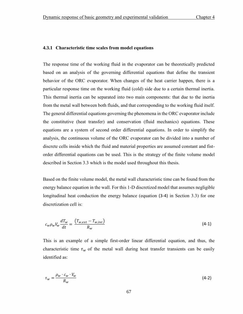
Dynamic response of basic geometry and experimental validation Chapter 4
67
4.3.1 Characteristic time scales from model equations
The response time of the working fluid in the evaporator can be theoretically predicted
based on an analysis of the governing differential equations that define the transient
behavior of the ORC evaporator. When changes of the heat carrier happen, there is a
particular response time on the working fluid (cold) side due to a certain thermal inertia.
This thermal inertia can be separated into two main components: that due to the inertia
from the metal wall between both fluids, and that corresponding to the working fluid itself.
The general differential equations governing the phenomena in the ORC evaporator include
the constitutive (heat transfer) and conservation (fluid mechanics) equations. These
equations are a system of second order differential equations. In order to simplify the
analysis, the continuous volume of the ORC evaporator can be divided into a number of
discrete cells inside which the fluid and material properties are assumed constant and fist-
order differential equations can be used. This is the strategy of the finite volume model
described in Section 3.3 which is the model used throughout this thesis.
Based on the finite volume model, the metal wall characteristic time can be found from the
energy balance equation in the wall. For this 1-D discretized model that assumes negligible
longitudinal heat conduction the energy balance (equation (3-4) in Section 3.3) for one
discretization cell is:
𝑐𝑤𝜌𝑤𝑉𝑤𝑑𝑇𝑤
𝑑𝑡=
(𝑇𝑤,𝑒𝑥𝑡 − 𝑇𝑤,𝑖𝑛𝑡)
𝑅𝑤 (4-1)
This is an example of a simple first-order linear differential equation, and thus, the
characteristic time 𝜏𝑤 of the metal wall during heat transfer transients can be easily
identified as:
𝜏𝑤 =𝜌𝑤 ∙ 𝑐𝑤 ∙ 𝑉𝑤
𝑅𝑤 (4-2)

Dynamic response of basic geometry and experimental validation Chapter 4
68
The thermal resistance and volume of the wall, depend on the geometry of the wall. In case
of a simple rectangular plate, the characteristic time of the metal wall is
𝜏𝑤 =𝜌𝑤 ∙ 𝑐𝑤 ∙ 𝑡ℎ𝑤
2
𝑘𝑤=
𝑡ℎ𝑤2
𝛼𝑤 (4-3)
Where the thermal diffusivity 𝛼𝑤 of the material, which includes all the relevant properties
of the wall material for the transient analysis, is defined as:
𝛼𝑤 =𝑘𝑤
𝜌𝑤 ∙ 𝑐𝑤 (4-4)
Metal walls in heat exchangers are, however, more often, cylindrical, or with more complex
geometries such as finned surfaces. In this case the characteristic time from equation (4-3)
will only give a first-order approximation.
In case of the working fluid response time, the energy balance equation on the working
fluid is more complex, being a non-linear differential equation. For the case of the 1-D
discretized model, the energy balance in each cell (equation (3-2) in Section 3.3) is:
𝑉 ∙ 𝜌(𝑇𝑤𝑓, 𝑝) ∙𝑑ℎ(𝑇𝑤𝑓 , 𝑝)
𝑑𝑡− 𝑉 ∙
𝑑𝑝
𝑑𝑡= �̇�𝑖𝑛 ∙ ℎ𝑖𝑛 − �̇�𝑜𝑢𝑡 ∙ ℎ𝑜𝑢𝑡 + 𝜃𝑤𝑓 ∙ 𝐴𝑖𝑛𝑡 ∙ (𝑇𝑤,𝑖𝑛𝑡 − 𝑇𝑤𝑓)
(4-5)
As it can be seen, this equation is more complicated since it a non-linear differential
equation. Since there is phase change happening as well, the equations of state relating the
different thermodynamic properties are discontinuous which leads to further complications.
Furthermore, the heat transfer correlation term is calculated based on semi-empirical or
fully empirical heat transfer correlations. This shows that in order to find a practical
solution for the calculation of the response times of the evaporator, it is more convenient
to use numerical approximations based on simulations of discretized models,

Dynamic response of basic geometry and experimental validation Chapter 4
69
4.3.2 Dynamic response from numerical simulations
Although a theoretical analysis of the governing equations of the phenomena present in the
ORC evaporator is an obvious starting point, it is not practical or even possible to obtain
exact results from an analytical solution since the mathematical model of the physics in the
ORC evaporator consists of non-linear equations. This is because the phenomena is a
complex, multi-variable, non-linear phenomena, and furthermore some semi-empirical
equations are required for the heat transfer correlations. A more pragmatic approach is
required for the investigation of the transient response. This involves the solving of the
equations numerically in a computational environment.
A method to identify the dynamics of any generic system is the one used in control theory
called system identification [157]. In that approach, the transient behavior of a dynamic
system is characterized by the output of a system to a certain input signal. This input-
output behavior is observed by means of an off-line or on-line test. In the on-line test, a
change in a certain variable (input) is applied to the physical system and the behavior over
time of one or a system of measured variables (output) is observed and identified as the
dynamic response of the system. In the off-line test, an accurate model of the system is
used to simulate the input-output behavior of the real system instead.
Based on standard practice, the most common types of input signals for the identification
of dynamic systems include the step input, impulse input, ramp input and sinusoidal input
[158]. The step input signal is typically the basic type of signal used to characterize the
time domain response of the system. Another important signal is the sinusoidal input, and
the response to this type of signal is called the frequency response of the system.
An on-line system identification on a real physical ORC evaporator gives tentatively more
certainty over that one particular ORC evaporator due to the incapacity of any model to
completely capture with absolute precision all the parameters of the system. However, it is
purely based on empirical test and gives little insight into the physical phenomena and main

Dynamic response of basic geometry and experimental validation Chapter 4
70
influencing factors affecting the dynamic response. Furthermore, if general conclusions are
to be drawn for different sizes, materials, boundary conditions or other parameters of ORC
evaporators, it might be impractical to build several physical systems to obtain general
trends of the dynamic response behavior.
Therefore, an ORC evaporator model based on the governing equations can provide insight
into the physical phenomena happening and how it affects the dynamic response.
Furthermore, it has the flexibility of being able to change at will certain parameters, while
keeping others fixed, and investigate the sensitivity that the dynamic response has on that
parameter. The model can be solved numerically with the help of a computer environment.
A drawback of using only simulation models is that there is an uncertainty on its accuracy.
Therefore, to increase the confidence on the results based on the model, a certain degree of
verification based on experimental results is required. This validation is presented in the
next section for the model used in this work.
4.4 Experimental validation of basic geometry model
The test rig that has been described in Section 3.7 is used to validate the model of the basic
ORC geometry. It consists of a closed loop of an organic fluid, with an emphasis on the
evaporator, where the organic working fluid enters at sub-cooled liquid state and gets
vaporized and slightly super-heated by heat transferred from an external hot air flow. The
organic working fluid utilized in the experiments is R245fa which is a well-known fluid
for ORC applications in the lower and medium temperature range. Furthermore, R245fa is
the main organic fluid considered in the case studies presented in this thesis.
An experimental campaign has been performed by applying different varying temperature
profiles of the air at the inlet of the evaporator. According to what has been described in
Section 4.3.2, step changes and sinusoidal profiles are very useful to extract the behavior
of dynamic systems. Sinusoidal profiles of the inlet air temperature where achieved by
continuous ramp-up and ramp-down of the air heater. However, due to hardware limitations

Dynamic response of basic geometry and experimental validation Chapter 4
71
(such as the hot air flowing in a closed loop), infinitely small changes of air inlet
temperatures are not physically possible and thus, air inlet temperature ramps where used
to approximate the step response behavior. The blower providing the air flow rate was kept
at constant speed during all experiments, however some variations of the flow rate were
inevitable due to the changing properties of the air with temperature such as the density.
Figure 4-2 shows an example of the measured hot air temperature and mass flow at the
inlet of the evaporator for the two types of experiment: the sinusoidal profile and the
trapezoidal (ramps) profile. The trapezoidal profile approximates the step response by
providing a fast ramp-up followed by a plateau and a fast ramp-down followed by an
extended valley.
Figure 4-2 Examples of different air flow and temperature inputs for experimental campaign (a)
Sinusoidal temperature profile (b) Trapezoidal temperature profile.
The sinusoidal input profiles provide a temperature fluctuation with an amplitude of
approximately 40 °C and three different frequencies. From the start to approximately 5000
s the fluctuation frequency is 1.67 mHz (a cycle period of 10 minutes), from ∼5000s to
∼8500 s, the fluctuation frequency is 1.04 mHz (a cycle period of 16 minutes) and from
∼8500s to the end the frequency is 2.78 mHz (a cycle period of 6 minutes)
The trapezoidal profiles consists of periodic temperature ramps (up and down) with periods
Sinusoidal profile Trapezoidal profile
(a) (b)

Dynamic response of basic geometry and experimental validation Chapter 4
72
of constant temperature in between. The ramp-up involves the increase of the air
temperature by 20 °C in 2 minutes time. Due to cooling of air limitations in the test rig, the
ramp-down to decrease the air temperature by 20 °C could only be performed in 4 minutes.
One constraint imposed on the profiles of the temperature and mass flow of the air is that
the thermal power available is able to ensure a slightly super-heated outlet state of the
working fluid (between 1 to 10 °C super-heating).
Both sinusoidal and trapezoidal profiles of the hot air tests were performed in the lab for
several pressures (and saturation temperatures) of the working fluid. The evaporator
pressure is manipulated by manually opening or closing the throttle valve at the outlet of
the evaporator. Tests at approximate evaporator pressures of 8, 10, 12 and 15 bars have
been performed. In this way the model can be validated for different sets of conditions. The
average inlet temperature of the working fluid for all test is 55 °C with minor fluctuations.
The volumetric flow provided by the pump for all tests is around 0.8 to 1 L/min.
The measurements from all the experiments on the test rig are used to validate the dynamic
model of the basic geometry. The model is described in detail in Section 3.3 with the
discretized cells interconnected in the way shown in Figure 3-4. As mentioned previously,
the model uses the modelling language Modelica and the simulation interface software
Dymola. The exterior heat transfer area is calculated with the inclusion of the fin
augmented area ratio 𝐴𝑜/𝐴𝑖. The model considers the thermal inertia of both the metal wall
and the fins. It has to be noted that the thermal inertia of the fins in the test-rig evaporator
is considerable and larger than the metal wall due to the large volume of the fin profile (see
Figure 3-9).
Figure 4-3 shows a schematic of the graphical interface of the evaporator model for
validation in Dymola. The inputs to the model consists of the measured inlet conditions
(flow rates and temperatures) of both the air and the organic working fluid. The detailed
geometric dimensions of the heat exchanger are also provided and are equal to the ones
presented in Table 3-5. A simple model of a throttle valve is described in Section 3.4.4 is

Dynamic response of basic geometry and experimental validation Chapter 4
73
included after the evaporator and the measured pressure after the throttle valve is provided.
The only parameter that is estimated is the throttle valve effective area which is adjusted
in order to provide the measured evaporator pressure values. The model considers the fluid
properties of both the organic working fluid R245fa and the external fluid air according to
the TIL Media library properties.
Figure 4-3 Graphical interface of evaporator model validation in Dymola.
Figure 4-4 shows some of the results of the Dymola model validation for one of the
sinusoidal profile experiments, the one performed with the profile presented in Figure 4-2a.
The evaporator pressure for this experiment was set around 12 bar. The results show the
main variables of interest from the parameters that were measured in the test and are not
inputs to the model. These include the temperatures of the working fluid and air at the
outlet of the evaporator as well as the working fluid pressure and an intermediate
temperature of the working fluid inside the evaporator (for the location of the
thermocouples refer to Figure 3-8).
As it can be seen there is a general agreement of the measured variables to the ones
provided by the simulation. There are only very small quantitative mismatches, particularly

Dynamic response of basic geometry and experimental validation Chapter 4
74
for the working fluid temperatures and pressure. Importantly, qualitatively the general
shape and amplitude of the model results are nearly identical compared to the experiments,
which shows that the model predicts accurately the transient behavior of the heat exchanger.
The air outlet temperature is the measurement that shows a higher quantitatively
discrepancy for this test. This can be attributed to the fact that the thermocouple at the air
side outlet is located after a bent in the piping causing a slight variation in the dynamic
pressure of the flow which is not accounted for in the model. Nevertheless, it has to be
noted that the error is of around 10 °C, which in the absolute temperature scale is less than
3%. Qualitatively, the general shape and amplitude of the fluctuations shows a very
accurate match with the experimental one.
Figure 4-4 Comparison of variables measured in the experiments to simulation results for the
sinusoidal input profile of Figure 4-2a with an evaporator pressure around 12 bar.
R245fa outlet temperature R245 outlet pressure
(a) (b)
Air outlet temperature R245fa intermediate temperature (TC4)
(c) (d)

Dynamic response of basic geometry and experimental validation Chapter 4
75
Table 4-1 summarizes the statistical errors of the simulation model values to the measured
values in all the experiments with input sinusoidal profiles. The errors are defined as the
deviation for each point in time 𝑘 between the measured value of the variable �̃�𝑘 and the
value of the variable from the simulation 𝜉𝑘 . The four statistical errors consist of the
maximal absolute deviation ∆𝜉𝑚𝑎𝑥, defined as:
∆𝜉𝑚𝑎𝑥 = 𝑚𝑎𝑥 [√(𝜉𝑘 − 𝜉𝑘)2] (4-6)
the maximal relative deviation ∆𝜉𝑚𝑎𝑥,𝑟𝑒𝑙 defined as:
∆𝜉𝑚𝑎𝑥,𝑟𝑒𝑙 = 𝑚𝑎𝑥
[ √(𝜉𝑘 − 𝜉𝑘)
2
𝜉𝑘
]
(4-7)
the average absolute deviation ∆𝜉̅ for an 𝑛 number of time points defined as:
∆𝜉̅ =
∑ [√(𝜉𝑘 − 𝜉𝑘)2]𝑛
𝑘
𝑛
(4-8)
and the average relative deviation ∆𝜉�̅�𝑒𝑙 defined as:
∆𝜉�̅�𝑒𝑙 =
∑ [√(𝜉𝑘 − 𝜉𝑘)
2
𝜉𝑘]𝑛
𝑘
𝑛
(4-9)
The errors are included for all the measured variables that are not inputs to the model.
These are the outlet temperature of the working fluid in the evaporator 𝑇𝑜𝑢𝑡,𝑤𝑓, the outlet

Dynamic response of basic geometry and experimental validation Chapter 4
76
pressure of the working fluid in the evaporator 𝑝𝑜𝑢𝑡,𝑤𝑓, the outlet temperature of the air in
the evaporator 𝑇𝑜𝑢𝑡,𝑔𝑎𝑠, and the intermediate temperatures of the working fluid inside the
evaporator 𝑇2,𝑤𝑓, 𝑇3,𝑤𝑓,𝑇4,𝑤𝑓 (for the location of the thermocouples refer to Figure 3-8).
Table 4-1 Statistical errors between simulation and experimental results for inputs of sinusoidal
profiles.
Experiments
identifier Variable ∆𝜉𝑚𝑎𝑥 ∆𝜉𝑚𝑎𝑥,𝑟𝑒𝑙 ∆𝜉̅ ∆𝜉�̅�𝑒𝑙
Experiments
A
Evaporator
Pressure
∼8 bar
𝑇𝑜𝑢𝑡,𝑤𝑓 20.7441 5.76% 7.811 2.14%
𝑝𝑜𝑢𝑡,𝑤𝑓 0.7803 9.43% 0.142 1.61%
𝑇𝑜𝑢𝑡,𝑔𝑎𝑠 9.3903 2.45% 5.683 1.48%
𝑇2,𝑤𝑓 19.9936 5.65% 11.324 3.17%
𝑇3,𝑤𝑓 22.6831 6.39% 13.215 3.70%
𝑇4,𝑤𝑓 26.5420 7.51% 16.180 4.54%
Experiments
B
Evaporator
Pressure
∼10 bar
𝑇𝑜𝑢𝑡,𝑤𝑓 15.2272 3.95% 2.288 0.61%
𝑝𝑜𝑢𝑡,𝑤𝑓 1.0766 9.97% 0.154 1.45%
𝑇𝑜𝑢𝑡,𝑔𝑎𝑠 14.8220 3.85% 10.391 2.69%
𝑇2,𝑤𝑓 13.1245 3.63% 5.235 1.44%
𝑇3,𝑤𝑓 16.5963 4.61% 6.628 1.82%
𝑇4,𝑤𝑓 18.1709 5.02% 7.842 2.16%
Experiments
C
Evaporator
Pressure
∼12 bar
𝑇𝑜𝑢𝑡,𝑤𝑓 10.3944 2.66% 2.114 0.56%
𝑝𝑜𝑢𝑡,𝑤𝑓 2.4172 15.88% 0.300 2.24%
𝑇𝑜𝑢𝑡,𝑔𝑎𝑠 12.6498 3.25% 9.678 2.49%
𝑇2,𝑤𝑓 52.2705 14.92% 8.586 2.34%
𝑇3,𝑤𝑓 54.7556 15.56% 9.615 2.61%
𝑇4,𝑤𝑓 5.6193 1.50% 3.004 0.80%
Experiments
D
Evaporator
Pressure
∼15 bar
𝑇𝑜𝑢𝑡,𝑤𝑓 11.0151 2.81% 2.257 0.57%
𝑝𝑜𝑢𝑡,𝑤𝑓 3.5812 22.01% 0.532 3.47%
𝑇𝑜𝑢𝑡,𝑔𝑎𝑠 22.2110 5.78% 7.755 1.99%
𝑇2,𝑤𝑓 21.5322 5.72% 11.819 3.13%
𝑇3,𝑤𝑓 23.1156 6.14% 13.626 3.60%
𝑇4,𝑤𝑓 22.3915 5.91% 12.541 3.30%

Dynamic response of basic geometry and experimental validation Chapter 4
77
It can be observed from Table 4-1 that the average relative errors of the model for all tests
performed under sinusoidal profiles is less than 5% and most are below 3.5%. The average
relative error of the outlet temperature of the working fluid is less than 1% except for the
tests at 8 bar where it is less than 2.5%. This small error gives confidence on the analysis
of the following chapters where the transient thermal condition on the working fluid side
is prominent.
Please note that the magnitude maximum absolute deviations are at times much larger than
the average values. This is because the maximum absolute deviation represents the single
measurement that deviates the most from the experimental data, a single measurement that
at times is an outlier that differs significantly from most of the measurements. This can be
due to faulty data, local momentary overheating/ pressure drop, instrument accuracy error,
among other factors. Outliers are expected in any experimental with a large sample, but
nevertheless must be reported.
Figure 4-5 shows the validation of the Dymola model for one of the experiments with the
air inlet trapezoidal temperature, in this case for the one performed with the profile
presented in Figure 4-2b. The evaporator pressure for this experiment was set around 15
bar. In order to observe, in detail, the different fast ramp changes (approximating step
changes), Figure 4-6 shows a close-up of the measured and simulated working fluid outlet
temperature after the four ramp-ups of Figure 4-2b have been applied.

Dynamic response of basic geometry and experimental validation Chapter 4
78
Figure 4-5 Comparison of variables measured in the experiments to simulation results for the
trapezoidal input profile of Figure 4-2b with an evaporator pressure around 15 bar.
It can be seen on both Figures that again there is both a good quantitative and qualitative
agreement on the results of the model compared to the measured values. The quantitative
agreement can be seen in Table 4-2, that summarizes the four more important statistical
errors on the model values compared to the experimental value for all the experiments with
trapezoidal input profiles. There is overall an average relative error of less than 3.5% for
all measured variables and less than 1% for the outlet temperature of the working fluid. In
Figure 4-5d it can be observed that there is a larger systematic deviation for the
intermediary temperature at the location of thermocouple number 2. In general, there are
R245fa outlet temperature R245 outlet pressure
(a) (b)
Air outlet temperature R245fa intermediate temperature (TC2)
(c) (d)

Dynamic response of basic geometry and experimental validation Chapter 4
79
larger errors in all the intermediary temperatures in the heat exchanger compared to the
outlet temperature. These larger errors in the intermediary temperatures can be explained
due to the fact that the model considers a number of discrete cells, inside which the fluid
properties are considered constant. Therefore, the model considers a series of discrete
values of temperature instead of the real continuous variation. If the location of the
thermocouple is, for instance, near to a border between two cells, a small error of the
measured temperature compared to the model value is expected. Nevertheless,
quantitatively, all the average relative errors of the intermediary temperatures are less than
5% which can be considered acceptable.
Figure 4-6 Four different expanded details of Figure 4-5a highlighting the comparison of measured
to simulation values for the four different temperature ramp-ups in the experiment.
R245fa outlet temperature R245fa outlet temperature
(a) (b)
R245fa outlet temperature R245fa outlet temperature
(c) (d)

Dynamic response of basic geometry and experimental validation Chapter 4
80
Table 4-2 Statistical errors between simulation and experimental results for inputs of trapezoidal
profiles.
Experiments
identifier Variable ∆𝜉𝑚𝑎𝑥 ∆𝜉𝑚𝑎𝑥,𝑟𝑒𝑙 ∆𝜉̅ ∆𝜉�̅�𝑒𝑙
Experiments
A
Evaporator
Pressure
∼8 bar
𝑇𝑜𝑢𝑡,𝑤𝑓 16.45 4.59% 2.82 0.77%
𝑝𝑜𝑢𝑡,𝑤𝑓 1.36 16.46% 0.17 1.99%
𝑇𝑜𝑢𝑡,𝑔𝑎𝑠 21.91 5.72% 15.16 3.95%
𝑇2,𝑤𝑓 15.39 4.35% 4.65 1.30%
𝑇3,𝑤𝑓 17.77 5.01% 5.60 1.56%
𝑇4,𝑤𝑓 21.00 5.94% 8.10 2.27%
Experiments
B
Evaporator
Pressure
∼10 bar
𝑇𝑜𝑢𝑡,𝑤𝑓 7.06 1.93% 1.55 0.41%
𝑝𝑜𝑢𝑡,𝑤𝑓 0.94 9.55% 0.16 1.52%
𝑇𝑜𝑢𝑡,𝑔𝑎𝑠 10.66 2.77% 6.78 1.76%
𝑇2,𝑤𝑓 11.84 3.27% 7.37 2.03%
𝑇3,𝑤𝑓 13.56 3.74% 9.21 2.53%
𝑇4,𝑤𝑓 15.02 4.14% 10.87 2.99%
Experiments
C
Evaporator
Pressure
∼12 bar
𝑇𝑜𝑢𝑡,𝑤𝑓 15.20 3.99% 2.31 0.61%
𝑝𝑜𝑢𝑡,𝑤𝑓 1.64 12.95% 0.28 2.18%
𝑇𝑜𝑢𝑡,𝑔𝑎𝑠 16.86 4.38% 5.71 1.47%
𝑇2,𝑤𝑓 21.92 5.94% 7.90 2.14%
𝑇3,𝑤𝑓 25.35 6.89% 10.81 2.93%
𝑇4,𝑤𝑓 23.83 6.42% 9.08 2.44%
Experiments
D
Evaporator
Pressure
∼15 bar
𝑇𝑜𝑢𝑡,𝑤𝑓 21.81 5.62% 2.41 0.62%
𝑝𝑜𝑢𝑡,𝑤𝑓 3.38 22.93% 0.38 2.43%
𝑇𝑜𝑢𝑡,𝑔𝑎𝑠 32.11 8.36% 7.50 1.92%
𝑇2,𝑤𝑓 29.02 7.74% 11.66 3.08%
𝑇3,𝑤𝑓 31.37 8.34% 13.03 3.43%
𝑇4,𝑤𝑓 31.53 8.34% 12.65 3.31%
Qualitatively, the match is also very satisfactory and gives a good confidence on the
capacity of the model to accurately predict transients. As it can be seen in all the
comparisons of Figure 4-6 the transient curve shape is almost identical for both the model

Dynamic response of basic geometry and experimental validation Chapter 4
81
result and the experimental measurements with slight differences in the magnitude of the
values.
It has to be noted the large thermal inertia of the test-rig evaporator. There is a relatively
large duration of the transient after the 2-minute ramp change in air temperature. In fact, it
takes around 600 s (6 minutes) for the temperature to reach within 95% of the final outlet
temperature (∼123 °C) from an initial temperature of around 118-120 °C. One important
factor for the large thermal inertia is the large volume of the fins, as it has been observed
that the response time of the model is significantly faster if the thermal inertia of the fins
is not considered. However, the large volume of the fins is not standard practice in heat
exchangers, and it is only the case for the test rig due to construction ease. Therefore, in
other geometries of real-case evaporators the thermal inertia is expected to be noticeably
lower.
One important consideration to take into account is that there is a limit in the accuracy of
all the test rig measurement devices (see Table 3-4). For instance, in general the average
errors of the outlet temperature of the working fluid in the validation are, in fact, within the
2.2 °C accuracy of the thermocouple.
Furthermore, any inaccuracy on any measurement of pressure, temperature or flow not only
affects directly the error of the aforementioned variable, but also affects indirectly all the
other variables, since the system is a highly-coupled multi-variable system. For instance,
an inaccuracy on the organic fluid value affects the evaporator pressure in the model, and
in turn the evaporator pressure on the model affects the saturation temperature and
ultimately the intermediate and outlet temperatures of the evaporator.
Because of all these reasons, the fact that the great majority of all the relative average errors
on the validation are below 3.5% is consider considerably good, and it is substantially
within the values that have been accepted as satisfactory in the validation of dynamic
models in the literature [64], [159].

Dynamic response of basic geometry and experimental validation Chapter 4
82
All the models throughout this thesis share the same basic structures as this validated model,
the only difference being the way the cells are interconnected and the calculation of the
geometric dimensions of interest. This gives a high level of confidence on the results based
on simulations for all types of heat exchangers in throughout this thesis.
4.5 A systematic characterization of response times of ORC evaporators
In the previous sections of this chapter, the basic geometry for ORC evaporators has been
described as well as the possible methods to characterize the dynamic behavior of the
evaporators. It has been concluded that numerical simulations based on discretized
mathematical models is the most convenient way to study the dynamics of ORC
evaporators. The discretized dynamic model of the evaporator has been validated against
experimental data showing good agreement at steady-state and during transients both
quantitatively and quantitatively.
Once the confidence on the dynamic model has been established, it can be used to provide
a more general analysis not bounded by the limitations of the evaporator on the test rig
which can only provide information on the dynamic behavior of only one group of
particular dimensions of a heat exchanger.
In this section, a systematic methodology to characterize and present the results of the
dynamic response of ORC evaporators in general is introduced. The main purpose of this
methodology is to be able to characterize the dynamics of ORC evaporators and to show
in the most general yet compact of ways the impact that the main variables have on the
dynamic response.
4.5.1 Characterization method
Based on the previously recommended approaches to characterize the response time of the
ORC evaporator, the method presented in Figure 4-7 is employed. Using the dynamic
model in the Modelica language described in Section 3.3, with the cell’s interconnection

Dynamic response of basic geometry and experimental validation Chapter 4
83
as in Figure 3-2 the dynamic response of the ORC evaporator to a step change of the heat
is investigated by simulating the dynamic model in the software Dymola. In order to reduce
the number of variables to a minimum, isolate the factors concerning only the working
fluid and metal wall and give more insight to the parameters that matter most, for this
fundamental case the heat carrier is replaced by a homogeneous heat flux in the exterior of
the tube wall.
The simulation of the model starts at a certain steady-state condition with a prescribed
degree of super-heating at the outlet of the working fluid side. Then, a step change of the
homogeneous heat flux is applied in the outer part of the tube wall while keeping all the
other boundary conditions fixed. The free response of the evaporator is then observed and
recorded in the simulation environment.
Since the outlet enthalpy is the property more representative of the thermal response of the
evaporator, it is chosen as the parameter that represents the dynamic response of the system.
The outlet enthalpy will gradually increase from the initial steady state and slowly converge
into a new steady state after the transient is over. This is represented in the right-hand graph
of Figure 4-7. The time when the outlet enthalpy reaches 95% of the new steady state is
defined as the response time 𝜏𝑒𝑣 This response time, in control terminology, is equivalent
to a rise time from 0 to 95% [158].
Figure 4-7 Dynamic response characterization schematic for simplified geometry.

Dynamic response of basic geometry and experimental validation Chapter 4
84
For a formal definition of the evaporator response time 𝜏𝑒𝑣, a dimensionless outlet enthalpy
can be defined as:
ℎ̃ = ℎ𝑜𝑢𝑡(𝑡) − ℎ𝑜𝑢𝑡(0)
ℎ𝑜𝑢𝑡(∞) − ℎ𝑜𝑢𝑡(0) (4-10)
The time zero is the time when the step change in the heat flux is applied. Using this
dimensionless enthalpy, the evaporator response time is formally defined as:
𝜏𝑒𝑣 = 𝑡(ℎ̃ = 0.95) (4-11)
From the validation in Section 4.4, it has been proven that the model can predict with
accuracy this response time for a real physical system,
4.5.2 Main factors affecting the response time
The evaporator response time 𝜏𝑒𝑣 depends mainly on the boundary conditions as well as
the thermal inertia of the metal wall and of the working fluid inside the tube. This thermal
inertia depend on the intensive properties, as well as the volume of wall material and
working fluid present. The intensive properties depend exclusively on the properties of the
selected wall material as well as the properties of the working fluid on the system, whereas
the volume depends on the geometry of the heat exchanger. The factors affecting the
thermal inertia of the evaporator can be then classified in the following three areas:
1) Geometry of heat exchanger. This affects the volume of both the wall material and the
working fluid. The geometry of the heat exchanger is chosen as to achieve a desired
heat transfer at design point. However, a different set of geometric dimensions can still
provide the same heat capacity 𝑈𝐴 of the heat exchanger, and thus the same heat
transferred in the heat exchanger at design point. For the case of the simplified
geometry considered in this chapter, and assuming the mass inertia of the fins as

Dynamic response of basic geometry and experimental validation Chapter 4
85
negligible there are three parameters required to define the geometry. The thickness of
the wall is usually defined by mechanical considerations. The other two are the tube
diameter 𝐷 and its length 𝐿. Both can be lumped into a geometric ratio 𝐷/𝐿.
2) Wall material thermal properties. The properties of the wall material that affect the
thermal inertia are the heat capacity 𝑐𝑤, the density 𝜌𝑤, and the thermal conductivity
𝑘𝑤, All these parameters can be lumped into the thermal diffusivity 𝛼𝑤, defined as:
𝛼𝑤 =𝑘𝑤
𝜌𝑤 ∙ 𝑐𝑤 (4-12)
3) Working fluid thermal properties. The selection of the working fluid often will be done
beforehand and obeys the suitability for the temperature of the heat source as well as
other considerations such as safety, environmental and other practicalities. The heat
capacity of the working fluid is different depending if it is in liquid, vapor or two-phase
state. One parameter that is of suitable interest that relates the heat capacities to the
latent heat of vaporization is the Jakob number 𝐽𝑎, defined as:
𝐽𝑎𝑙𝑣 =𝐶𝑝,𝑣(𝑇𝑣 − 𝑇𝑠𝑎𝑡) + 𝐶𝑝,𝑙(𝑇𝑠𝑎𝑡 − 𝑇𝑙)
∆𝐻𝑣𝑎𝑝 (4-13)
Where 𝐶𝑝,𝑣 and 𝐶𝑝,𝑙 are the specific heat capacities of the fluid at vapor and liquid phases
respectively, 𝑇𝑣 and 𝑇 are the initial outlet (super-heated vapor) and inlet (sub-cooled
liquid) temperatures, 𝑇𝑠𝑎𝑡 is the saturation temperature and ∆𝐻𝑣𝑎𝑝 is the enthalpy of
vaporization of the fluid.
4) Boundary conditions. The boundary conditions are the heat flux from the heat source,
the inlet thermal condition of the working fluid as well as the initial outlet condition of
the working fluid. The boundary conditions depend on the characteristic of the heat
source and the steady-state design of the system.

Dynamic response of basic geometry and experimental validation Chapter 4
86
4.5.3 Response time maps
In order to illustrate the dependence of the aforementioned factors on the response time of
ORC evaporators in a generalized way, a graphical method is proposed. The response time
of the basic geometry ORC evaporator is found by simulating the dynamic model with
varying values of the factors of interest. The results from several simulations are
interpolated and charts are built indicating curves of constant response time for different
varying factors in the x and y axis.
It has to be noted that certain factors and boundary conditions of an ORC evaporators are
defined and fixed by considerations such as the available thermal power and temperature
of the heat source and the thermodynamic cycle optimization. Therefore, some of them
cannot be changed, once the boundary conditions and the thermodynamic cycle are defined.
This can be called fixed parameters. However, there are others factors that can be
considered as degrees of freedom in order to modify the response time of the evaporator.
This can be called dynamic response parameters. For instance, the heat transfer area is
fixed parameter defined by the available thermal power of the source and the cycle
requirements. However, the geometric diameter to length ratio 𝐷/𝐿 of the heat exchanger
is not, and can be varied while still keeping the same heat transfer area.
Figure 4-8 shows the response time maps for the basic geometry as a function of the
dynamic response parameters. This include the geometric ratio 𝐷/𝐿 and the wall material
thermal diffusivity 𝛼𝑤 for two different values of the Jakob number. The maps are built for
the fixed parameters presented in Table 4-3 with R245fa as the working fluid.
Regarding the fixed parameters, in order to showcase in a general way qualitative trends,
in the maps of Figure 4-8 the heat transfer area is set as unitary, with a nominal heat flux
(heat transferred per area) observed from external gaseous flows (i.e. the heat flux observed
in the test rig), the wall thickness has a standard value of 0.02 mm. The evaporator pressure
is set at 15 bar with an initial super-heating value of 1 °C.

Dynamic response of basic geometry and experimental validation Chapter 4
87
It must be noted also that each of the two maps represent two different working fluid inlet
temperatures, which define the two different values of Jakob number. Since the inlet
temperature depends on the conditions of the condenser or on the design of a potential
recuperator, this is also shown as a potential decision factor or dynamic response parameter
that affects the dynamic behavior. The mass flow of the working fluid is adjusted for each
inlet temperature condition in order to achieve the same initial super-heating with the same
heat transfer area.
The two Jakob numbers selected for the response time maps, are exemplary of two different
inlet working fluid temperature conditions in the evaporator representing two different
configurations. The smaller Jakob number (𝐽𝑎𝑙𝑣= 0.593) represents an inlet temperature
(55 °C) that is probable for an ORC that includes a recuperator, while the larger Jakob
number (𝐽𝑎𝑙𝑣= 0.923) represents an inlet temperature (25° C) that is probable for an ORC
without a recuperator.
Table 4-3 Fixed parameters for response time maps of Figure 4-8
𝐽𝑎𝑙𝑣 Working
fluid
Heat
transfer
area
Wall
thickness
Saturation
pressure
Heat
flux
Initial
super-
heating
Inlet
temperature
working
fluid
Mass
flow
rate
0.593 R245fa 1 m2 2 mm 15 bar 7000 W/m2 1 °C 55 °C
0.34 kg/s
0.923 R245fa 1 m2 2 mm 15 bar 7000 W/m2
1 °C 25 °C 0.28 kg/s

Dynamic response of basic geometry and experimental validation Chapter 4
88
Figure 4-8 Response time maps for basic geometry with unitary heat transfer area for two different
Jakob numbers. Fixed parameters as in Table 4-3
From the response time maps of Figure 4-8 some general insight can be drawn on the
influence of each dynamic response parameter and their interactions:
• Geometric ratio 𝐷/𝐿. The response time is slower with an increasing value of 𝐷/𝐿.
This is because larger diameters with shorter lengths represent a higher volume of
the working fluid while still keeping the same heat transfer area. A larger volume
of the working fluid requires more time to reach a new steady state. There is an
enhanced variation of the response time with 𝐷/𝐿 for lower values of the the wall
material 𝛼𝑤
• Wall material thermal diffusivity𝛼𝑤. As expected a larger thermal diffusivity means
shorter response times. A material with higher values of 𝛼𝑤 allows for a faster heat
transfer and stores less thermal power during transients. A low value of 𝛼𝑤, makes
the response time more sensitive to changes in geometric dimensions.
• Fluid properties / thermal state represented by the Jakob number 𝐽𝑎𝑙𝑣. The Jakob
number 𝐽𝑎𝑙𝑣 is related in this case to the inlet temperature of the working fluid. For
𝑱𝒂𝒍𝒗 = 0.593 𝑱𝒂𝒍𝒗 = 0.923
(a) (b)

Dynamic response of basic geometry and experimental validation Chapter 4
89
the two 𝐽𝑎𝑙𝑣 considered the response time values are similar but differ specially on
the left top and right bottom corner. For low 𝐷/𝐿 and high 𝛼𝑤 the response time is
slower for the larger 𝐽𝑎𝑙𝑣 and the opposite is true for high 𝐷/𝐿 and low 𝛼𝑤. This is
confirmed by highlighting the deviation of the response time with the Jakob number
at is shown in Figure 4-9. It is clearly seen in Figure 4-9b that for a large thermal
diffusivity of the wall the response time is slower for the larger 𝐽𝑎𝑙𝑣 specially at
larger values of 𝐷/𝐿. The opposite is true in Figure 4-9a, representing a smaller
thermal diffusivity of the wall. In this case the response time is slower for the
smaller Jakob number. The latter case can be explained by the fact that the mass
flow of working fluid in the evaporator is less (see last column of Table 4-3). This
lower mass of fluid plays a major role when the volume of the heat exchanger is
larger as it is the case with higher 𝐷/𝐿. For low 𝐷/𝐿 the quantity of working fluid
has less of an impact on the thermal inertia and the dominant factor is the less
effective heat transfer for one-phase fluid which slows down slightly the dynamics.
Figure 4-9 Deviation of response time for the two Jakob numbers considered for two different
values of the thermal diffusivity of the wall material 𝜶𝒘, corresponding to common construction
materials (a) Steel and (b) Aluminium
𝜶𝒘 = 4.1 (Steel) 𝜶𝒘 = 86.5 (Aluminium)
(a) (b)

Dynamic response of basic geometry and experimental validation Chapter 4
90
It can be observed from the maps that the response time is most sensitive to the geometric
dimensions than to the other dynamic response parameters. In other words, this is the
parameter that can be changed to most effectively influence the dynamic response of the
system. The material of the wall comes in second place.
The response time maps also serve as a tool to customize the dynamic response of the
system. A faster response time may be required in order to achieve fast control, or rather a
large response time may be preferred in order to have a more robust system to sudden
changes of the heat source, and one that can dampen certain fluctuations.
The potential of the response time maps will be further highlighted in the following
Chapters where they will be expanded and used in practical cases to improve the dynamic
performance of ORC systems.
4.6 Summary
In this chapter a general analysis of the factors affecting the ORC evaporator response time
has been carried out for the case of a basic general geometry. Although an examination of
the formal governing equations is an important starting point to find the characteristic time
scales of the system, the phenomena is complex, multi-variable and non-linear and
ultimately simulation of models that utilize discretization methods prove more practical to
obtain meaningful results.
The level of confidence on the results based on these models is higher when some
validation based on experimental data is available. Because of that, this chapter has shown
a validation of the dynamic model used in Dymola by comparing simulation results to
measured data obtained during an extensive experimental campaign on a test rig in the
laboratory. The validation has shown that the model can accurately predict both
quantitatively and qualitatively the behavior of the ORC evaporator in the lab during
transients.

Dynamic response of basic geometry and experimental validation Chapter 4
91
With a high level of confidence on the dynamic model, a first glimpse into a methodology
to systematically characterize the dynamic response of ORC evaporator has been presented.
The concept of response time maps has been introduced, presenting its potential for
customization of the evaporator dynamic response. These concepts will be expanded and
applied to relevant situations in the next two chapters.


Dynamic behavior of heat exchangers for direct evaporation Chapter 5
93
Chapter 5 *
Dynamic behavior of different types of heat exchangers for
direct evaporation
This Chapter expands the concepts of response time maps introduced in the
previous Chapter to more complex geometries belonging to the real types
of heat exchangers that can be used for direct evaporation. The potential of
the methodology to customize the thermal inertia of the ORC system is shown
on the case of the profile of an IC engine exhaust during a standard driving
cycle. The concept of dynamic regimes is introduced and the dynamic regime
number is used as a tool to relate the response time of the evaporator with the
fluctuation characteristics of the heat source in order to obtain a certain
dynamic behavior.
________________
*This section published substantially as M. Jiménez-Arreola, R. Pili, C. Wieland, A.
Romagnoli. Analysis and comparison of dynamic behavior of heat exchangers for direct
evaporation in ORC waste heat recovery applications from fluctuating sources. Journal of
Applied Energy, Vol. 216, pp. 724-440, 2018

Dynamic behavior of heat exchangers for direct evaporation Chapter 5
94
5.1 Introduction
There are several different designs and types of heat exchangers that could be utilized as
ORC evaporators. Furthermore, more complex layouts including more than one heat
exchanger are usually chosen for practical considerations. That is the case of indirect
evaporation layouts, in which an intermediary heat transfer fluid is used to decouple the
heat transfer from the main heat source to the ORC working fluid.
Direct evaporation is the ORC layout in which only one heat exchanger is used to transfer
the heat directly from the main heat carrier of the heat source to the ORC fluid. Direct
evaporation is the most simple and efficient way to transfer heat to the ORC fluid, yet in
real practical applications that include high variability of the heat source is not often the
preferred choice. This is because indirect evaporation can more effectively protect the fluid
from extreme changes in the boundary conditions by damping the variability of the heat
source. The working fluid must be above saturation temperature and below chemical
decomposition temperature at the outlet of the evaporator at all times. As has been
explained previously in Chapter 2, the intermediary heat transfer loop in indirect
evaporation layouts can be considered a type of sensible heat thermal energy storage.
In this chapter, some relevant types of heat exchanger for direct evaporation are analyzed
based on their dynamic response to changes of the heat source. This analysis is done based
on the concepts introduced in Chapter 4. However, unlike Chapter 4, in this Chapter more
detailed models of heat exchangers with real-life complex geometries are analyzed. The
waste heat carrier properties are also taken into account.
In waste heat recovery applications, the heat carrier is most often a gaseous fluid (i.e. an
engine exhaust). Due to the lower heat transfer coefficient of gases compared to the
evaporative heat transfer coefficient, a good way to ensure the compactness and
effectiveness of the direct evaporation heat exchanger is to have extended surfaces on the
gas side. Therefore, in this Chapter, the analysis is restricted to the types of heat exchangers
that are suitable for direct evaporation in most practical cases. Two different types are

Dynamic behavior of heat exchangers for direct evaporation Chapter 5
95
considered: a multiple fin and tube heat exchanger and a louver fin multi-port heat
exchanger.
5.2 System assumptions and characterization approach
As an illustrative and relevant case, the evaporators analyzed in this work are intended to
be a part of an ORC system recovering waste heat from the exhaust of a diesel engine. This
is a situation where direct evaporation can be an attractive option due to volume and weight
restrictions in mobile applications.
The study in this Chapter is intended for a high efficiency system. A schematic of the ORC
system is shown in Figure 5-1 along with a representative T-S diagram. An optional small
recuperator can be installed to increase the thermal efficiency and decrease the size of the
evaporator.
Figure 5-1 (a) Schematic of ORC under investigation (b) Qualitative T-S diagram of the process.
(a) (b)

Dynamic behavior of heat exchangers for direct evaporation Chapter 5
96
The working fluid considered is the benchmark R245fa, which is suitable for the
temperatures and mass flows available in this type of applications [160]. Furthermore,
R245fa is a well-known and widely used fluid in ORC systems and it’s the fluid used in
the research papers in which the ORC evaporator geometries of this work is based [58],
[131].
The exhaust gas boundary conditions are assumed based on the range of values reported
by Yang et. al [58] for a six-cylinder in line Diesel engine with rated power of 240 kW.
They represent values for the exhaust on the medium to high torque. The composition of
the exhaust is taken as the combustion gas of a diesel fuel with an air-fuel equivalence ratio
λ of equal to 1.2. The inlet conditions of the exhaust for the base case are reported in Table
5-1.
As per the working fluid, the conditions at the inlet of the evaporator will depend on the
dynamic conditions in the condenser and, if it is the case, the recuperator. The working
fluid inlet temperature is treated as one of the parameters to be studied. For the base case
it is assumed a fixed value of the inlet conditions in the evaporator of 10 below the
saturation temperature. Furthermore, it is assumed that the working fluid is completely
evaporated and super-heated to 1 °C above the saturation temperature. This is because low-
super-heating allows for higher efficiencies when using organic fluids with high molecular
weights such as R245fa [75]. The working fluid boundary conditions at base case are also
reported in Table 5-1.
As it has been done in Chapter 4 the dynamic response of the evaporators is characterized
by its transient response to a step change on the heat conditions. As defined in Chapter 4
the response time 𝜏𝑒𝑣 of the evaporator is the time it takes to rise to 95% of the new steady
state when subjected to a step change of either the mass flow or the temperature of the
engine exhaust.
Figure 5-2 shows the schematics of the characterization approach. The model in Dymola
starts at a steady state with given initial parameters. At a certain time, a step change on

Dynamic behavior of heat exchangers for direct evaporation Chapter 5
97
mass flow or temperature of the exhaust is imposed. The simulation is carried out during
the subsequent transient until a new steady state is reached. The response time 𝜏𝑒𝑣 is
recorded.
Table 5-1 Boundary conditions and fluid descriptions in ORC evaporator for the base case.
Description Value
Exhaust inlet temperature 350 °C
Exhaust inlet pressure 1 bar
Exhaust mass flow 0.35 kg/s
Working fluid inlet temperature 133 °C
Working fluid inlet pressure 30 bar
Working fluid initial degree of super-heating
at outlet 1 °C
Working fluid R245fa
Exhaust properties Combustion gas λ = 1.2
Figure 5-2 Dynamic response characterization approach.

Dynamic behavior of heat exchangers for direct evaporation Chapter 5
98
5.3 Heat exchanger geometries
Figure 5-3 shows the geometry and main dimensional parameters of fin and tube heat
exchangers. The base case dimensions for this study are based on the real heat exchanger
dimensions reported by Yang et al. [58] and reported in Table 5-2. The referred heat
exchanger has been dimensioned considering the base boundary conditions of Table 5-1.
Figure 5-4 shows the geometry and main dimensional parameters of the louver fin multi-
port flat tubes heat exchanger. For this type of heat exchanger, the base geometric
dimensions are based on the one reported by Mastrullo et al. [131]. The base case
dimensions are reported in Table 5-3.
.
Figure 5-3 Geometry of fin and tube heat exchanger.

Dynamic behavior of heat exchangers for direct evaporation Chapter 5
99
Table 5-2 Dimensions of fin and tube heat exchanger at base case.
Description Value
Number of tube banks 20
Number of tubes per bank 9
Tubes inner diameter 20 mm
Tube length 800 mm
Tube thickness 2.5 mm
Clearance between tube banks 35 mm
Clearance between tubes per bank 75mm
Fin height 12 mm
Fin thickness 0.1 mm
Fin pitch 2 mm
Tube banks arrangement Staggered
Tube and fin material Stainless steel
Figure 5-4 Geometry of louver fin multi-port heat exchanger.

Dynamic behavior of heat exchangers for direct evaporation Chapter 5
100
Table 5-3 Dimensions of louver fin multi-port heat exchanger at base case.
Description Value
Number of ports per tube 20
Number of flat tubes 7
Port inner diameter 2 mm
Tube length 840 mm
Port wall thickness 2.5 mm
Clearance between ports 35 mm
Clearance between tubes 75 mm
Fin thickness 0.5 mm
Fin pitch 2 mm
Louver angle 25 °
Louver pitch 0.8 mm
Tube and fin material Stainless steel
5.4 Parameters of interest
As explained in Chapter 4, the main aspects that affect the dynamic response of the
evaporator can be grouped in the following areas: wall material, boundary conditions and
geometry. Of these, the first two can be manipulated at the design stage, whereas the third
aspect also depends on the operational characteristics at a given time.
In order to study the response time dependence on these different areas for each of the heat
exchanger types, a parametric study is carried out where the dynamic characterization is
performed for various series of combinations of the studied parameters. A description of
each of these parameters is given below:
5.4.1 Wall material
The simulations are carried out for different relevant engineering materials for the heat
exchanger walls. These include, stainless-steel, aluminum and copper. To draw general

Dynamic behavior of heat exchangers for direct evaporation Chapter 5
101
conclusions, the thermal diffusivity 𝛼𝑤 of the material is used as the parameter of interest.
As it has been shown in Chapter 4 it is defined as:
𝛼𝑤 =𝑘𝑤
𝜌𝑤 ∙ 𝑐𝑤 (5-1)
As it has been explained in Chapter 4, this parameter includes all the relevant material
properties for the transient analysis in solids.
5.4.2 Boundary conditions
The boundary conditions are varied reflecting the changing conditions of the heat source
and working fluid according to a range of values expected during operation. Three different
varying conditions are varied: exhaust inlet temperature, exhaust mass flow, and working
fluid inlet temperature. It is to be noted that in these simulations the working fluid mass
flow is automatically determined by the requirement that the outlet conditions is 1 °C of
super-heating. This is equivalent to assume there is a perfect controller that changes the
working fluid mass flow to reach a given super-heating set point.
5.4.3 Geometric dimensions
The geometry of the heat exchanger has been found in Chapter 4 to have a higher impact
on the dynamic response as compared to the wall material. Therefore, it is the most
important design aspect that should be the focus on tailoring the dynamic response of the
system.
Since both types of heat exchangers have complex geometries, only the main geometric
dimensions are studied. In this analysis, the tubes and ports clearances and the fins
geometries are kept fixed at the base design values. The dimensions that are varied include
the tube or port diameter and the parameters that affect the three main volume dimensions.
For fin and tube heat exchangers the varied dimensions are the diameter of tubes, the

Dynamic behavior of heat exchangers for direct evaporation Chapter 5
102
number of tubes banks (number of tubes in the direction parallel to the exhaust flow), the
number of tubes per bank (number of tubes in the direction perpendicular to the exhaust
flow) and the length of the tubes.
For louver fin multi-port heat exchangers, the corresponding geometric dimensions are the
port diameters, the number of ports, the number of flat tubes and the length of flat tubes.
However, for each type of heat exchanger, the four dimensions are not independent of each
other. In order to properly and independently assess how the different aspects affect the
dynamic response, the thermal capacity 𝑈𝐴 of the heat exchanger must be fixed. In this
way, the same heat transferred and the same output properties the fluid at steady state are
achieved for a given set of boundary conditions. Therefore, if one of the geometric
parameters is varied while keeping the others fixed, one other dimension must change in
order to keep the same thermal capacity of the heat exchanger and the same outlet thermal
condition of the working fluid. Since the diameter is the geometrical dimension that has a
larger effect on the heat transfer and the response time, it is decided to vary each of the
other dimensions independently and always adjust the tube or port diameter accordingly.
This is summarized in Table 5-4.
Table 5-4 Different cases of geometric dimensions varied in the simulations for each type of heat
exchanger.
Heat exchanger type Case Parameter varied Parameter adjusted
to keep same 𝑈𝐴
Fin and tube
1 No. of tube banks Tube inner diameter
2 No. of tubes per bank Tube inner diameter
3 Tube length Tube inner diameter
Louver fin multi-port
1 No. of ports per tube Port diameter
2 No. of tubes Port diameter
3 Tube length Port diameter

Dynamic behavior of heat exchangers for direct evaporation Chapter 5
103
5.5 Response time maps
The results of the parametric simulations are compiled and interpolated in order to develop
general the maps of the response time for both heat exchangers in terms of evaporator
design and boundaries parameters. As it has been introduced in Chapter 4, the response
time maps represent a guide showing what it takes, in terms of design of the heat exchanger,
to achieve the desired thermal inertia of thee evaporator.
It has been found that the response time of the evaporator to step changes in temperature
is very similar to the case of step changes in exhaust mass flow rate. The results of the
simulations show a variation of less than 5% on the response time in the case of 10 °C step
change in comparison to the case of 10% step change of mass flow rate for all simulation
points considered. Because of this, the response time maps for the case of step changes in
exhaust temperature are excluded from this analysis since step changes in mass flow rate
are sufficient enough to characterize the dynamic response times of the heat exchangers in
a general way.
Therefore, the results shown correspond to 10% step change of mass flow rate. Response
time maps have been built for a different combination of the main parameters of interest
described in Section 5.4. Below a detail description and discussion of each case.
5.5.1 Geometry and wall material
Figure 5-5 presents the response time maps showing the dependence that the evaporator
response time has on the different heat exchanger design parameters for each type of heat
exchangers. The x-axis corresponds to a variation in the geometry while the y-axis to a
variation in the wall material represented by its thermal diffusivity 𝛼𝑤. Two x-axes are
shown, the bottom x-axis shows the geometric parameters varied (number of tubes, length,
etc.) while the main x-axis shows the corresponding adjusted value of tube/port diameter
(to keep same thermal capacity). In order to correlate the y-axis values to some relevant
engineering materials, Table 5-5 summarizes the thermal diffusivity of some materials that

Dynamic behavior of heat exchangers for direct evaporation Chapter 5
104
can be used to build the heat exchangers along with their main thermal properties.
The geometry and material of the heat exchanger not only affect the thermal response time
of the evaporator but also the volume and mass of heat exchanger. This is especially
relevant for mobile applications and others with size restrictions. The material mass also
represents some of the material costs implication when changing the geometry. Figure 5-6
shows how the volume and mass of the evaporator is affected by the corresponding changes
in geometry for three wall materials of interest.
From the maps it can be seen that the variation of the diameter of the working fluid conduit
is the dominant parameter that modifies the response time of the evaporator, whereas the
thermal properties of the wall material play a smaller role. As expected, a higher thermal
diffusivity of the material reduces the response time due to a faster heat conduction through
the wall. Larger diameters increase the quantity of the working fluid present in the
evaporator at a given time and therefore, because a larger mass of fluid needs to be heated
up to the next steady state, the thermal inertia and response time of the evaporator is
increased.
In the case of fin and tube evaporators, for Figure 5-5c and e, the diameter similarly affects
the response time value regardless of the other geometric parameter that is varied. However,
in the case of Figure 5-5a, when the number of tube banks is varied, the response time is
slower at larger diameters and faster at smaller diameters in comparison. This is because
of the disparity in the trend of mass variation that the evaporator has when the number of
tube banks is varied as compared to the other two cases. This can be observed in Figure
5-6a.
For louver fin multi-port evaporators, Figure 5-5b and d have similar trends of the response
time variation when the diameter is varied, while Figure 5-6f, which corresponds to a
variation of tube length, has a different trend. This is also because of the variation of mass
when the tube length changes is different than the two other cases as observed in Figure
5-6b.

Dynamic behavior of heat exchangers for direct evaporation Chapter 5
105
From this analysis, it is concluded that both a larger amount of fluid and a larger amount
of material of the heat exchanger increases the response time. However, the dominant effect
is the volume of the working fluid.
5.5.2 Geometry and exhaust boundary conditions
The exhaust boundary conditions are constantly varying according to the operational point
of the engine. Apart from the thermal power fluctuations, the mean value of the mass flow
or temperature of the exhaust around which the fluctuations happen can also vary.
Therefore, it is important to consider also how the mean value affects the response.
Figure 5-7 shows the variation of the evaporator response time maps for different exhaust
mass flow rates corresponding to the different geometric dimensions. Figure 5-8 shows the
response time maps in case of different temperature of exhaust and the different geometric
dimensions. The maps also include the corresponding pressure drops for the working fluid
and the exhaust in the evaporator, highlighting to the heat exchanger designer the penalties
and benefits in pressure drops related to a certain design with a given response time.
In the model, the mass flow of the working fluid is adjusted according to the different
boundary conditions to achieve the requirement of 1 °C of initial super-heating at the outlet
of the evaporator. The values of the working fluid mass flow for the different values of
boundary condition are summarized in Table 5-6. The parametrization is done around the
base case values of Table 5-1.
As seen in Figure 5-7 and Figure 5-8, higher flow or temperature of the heat source reduces
the response time of the evaporator. This is because with higher mass flow or temperatures
of the exhaust, the heat available is higher and the mass flow of the working fluid required
to achieve 1 °C super-heating at the outlet is higher. The higher the mass of the working
fluid at a given time results in higher thermal inertia of the system.

Dynamic behavior of heat exchangers for direct evaporation Chapter 5
106
For fin and tube evaporators, the response time for a tube diameter of 0.02 m reduces from
88 s with an exhaust mass flow of 0.2 kg/s to 45 s with an exhaust mass flow of 0.4 kg/s.
In the case of different exhaust temperature, the response time for a tube diameter of 0.02
m reduces from about 97 s at an exhaust temperature of 250 °C to 43 s at an exhaust
temperature of 400 °C. For both cases, the reduction gradient in the maps is increased with
larger diameter, resulting in similar percentage reduction. In general, the response time
reduces approximately 30% per 0.1 kg/s increase in exhaust mass flow and reduces
approximately 30% for 50 °C increase in exhaust temperature.
For louver fin multi-port evaporator with a port diameter of 2 mm, the response time
decreases from 30 s at an exhaust mass flow rate of 0.2 kg/s to 20 s at 0.4 kg/s and decreases
from 35 s at an exhaust temperature of 250 °C to 18 s at 400 °C. In general, the response
time reduces approximately 20% per 0.1 kg/s increase in exhaust mass flow and reduces
approximately 20% per 50 °C increase in exhaust temperature.
5.5.3 Geometry and working fluid inlet condition
The inlet conditions of the working fluid in the evaporator also can vary due to changes in
the boundary conditions corresponding to a different operating point in the condenser on
in the optional recuperator. These variations are also considered and their effect on the
evaporator response time for different geometries is shown in the maps of Figure 5-9 for
the case of fin and tube heat exchangers.
In Figure 5-9 it is shown that the effect on the response time is more significant and
increases with a higher degree of sub-cooling of the fluid at the inlet. For instance, for a
tube diameter of 0.02 m the response time increases from about 40 s at 5 °C inlet sub-
cooling to 90 s at 30 °C inlet sub-cooling. This slower response is due to the fact that the
heat transfer in the one-phase region is slower than in the evaporation process. The gradient
of response time increase is higher at smaller degrees of sub-cooling and is similar to all
values of tube diameter.

Dynamic behavior of heat exchangers for direct evaporation Chapter 5
107
Figure 5-5 Effect of wall material thermal diffusivity 𝜶𝒘 and heat exchanger geometry on
evaporator response time for different varying conditions and a 10% step increase in exhaust mass
flow rate.
Fin and tube evaporator Louver fin multi-port evaporator
(a) (b)
(c) (d)
(e) (f)

Dynamic behavior of heat exchangers for direct evaporation Chapter 5
108
Figure 5-6 Weight and volume of evaporator for different varying geometric parameters – No. of
banks/ports, No. of tubes, Tube length- as function of their corresponding tube diameters. Wall
material: stainless steel (SS), aluminium (Al) and Copper (Cop). (a) Fin and tube heat exchanger
weight. (b) Louver fin multi-port heat exchanger weight. (c) Fin and tube heat exchanger volume.
(d) Louver fin multi-port heat exchanger volume.
Fin and tube evaporator Louver fin multi-port evaporator
(a) (b)
(c) (d)
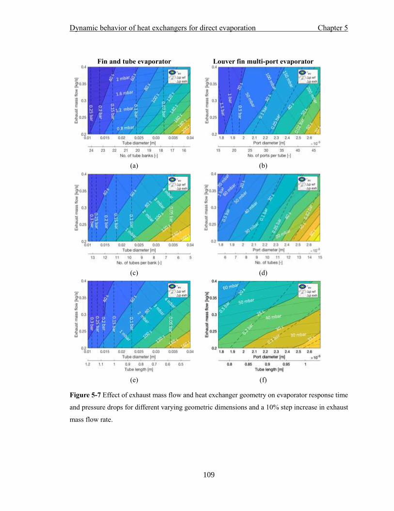
Dynamic behavior of heat exchangers for direct evaporation Chapter 5
109
Figure 5-7 Effect of exhaust mass flow and heat exchanger geometry on evaporator response time
and pressure drops for different varying geometric dimensions and a 10% step increase in exhaust
mass flow rate.
Fin and tube evaporator Louver fin multi-port evaporator
(a) (b)
(c) (d)
(e) (f)

Dynamic behavior of heat exchangers for direct evaporation Chapter 5
110
Figure 5-8 Effect of exhaust inlet temperature and heat exchanger geometry on evaporator response
time and pressure drops for different varying geometric dimensions and a 10% step increase in
exhaust mass flow rate.
Fin and tube evaporator Louver fin multi-port evaporator
(a) (b)
(c) (d)
(e) (f)

Dynamic behavior of heat exchangers for direct evaporation Chapter 5
111
Table 5-5 Relevant properties of wall materials considered, according to values of the TIL media
library [148]
Material
Thermal
conductivity
𝑘 [W/(m∙ K)]
Density 𝜌 [kg/m3]
Specific heat
capacity 𝑐
[J/(kg∙ K)]
Thermal
diffusivity 𝛼
[mm2/s]
Steel 14.6 7900 450 4.1
Aluminium 215 2700 920 86.5
Copper 398 8960 380 116.9
Table 5-6 Required working fluid mass flow rate as function of boundary conditions in order to
achieve 1 °C of initial super-heating at the outlet of the evaporator in the case of the base geometry
of fin and tube evaporator.
Exhaust inlet
mass flow [kg/s]
Exhaust inlet
temperature [°C]
Working fluid
inlet degree of
sub-cooling [°C]
Required working
fluid mass flow
[kg/s]
0.2 350 10 0.51
0.25 350 10 0.63
0.3 350 10 0.76
0.35 250 10 0.45
0.35 300 10 0.66
0.35 350 10 0.88
0.35 350 20 0.75
0.35 350 30 0.66
0.35 400 10 1.11
0.4 350 10 1.01

Dynamic behavior of heat exchangers for direct evaporation Chapter 5
112
Figure 5-9 Effect of working fluid inlet temperature and heat exchanger geometry on evaporator
response time and pressure drops for different varying geometric dimensions and a 10% step
increase in exhaust mass flow rate, for the case of fin and tube evaporator.
(a) (b)
(c)

Dynamic behavior of heat exchangers for direct evaporation Chapter 5
113
5.5.4 Implications for fin and tube heat exchangers
An evaporator with a larger thermal inertia may be desired in order to dampen fluctuations
of the thermal power. From the response time maps, it is clear that in order to increase the
thermal inertia of the evaporator, the most effective way is to increase the tube diameter.
For the fin and tube heat exchangers in this study, in order to keep the same thermal
capacity 𝑈𝐴 of the heat exchangers an increase in tube diameter requires a reduction of
number of tubes or of tube length. Large tube diameter reduce the Reynolds number and
heat transfer coefficient but increase significantly the heat transfer area per tube. The
reduction of number of tubes or tube length balances the increase in heat transfer area.
As seen in Figure 5-6a, the overall weight of the heat exchanger increases with a larger
diameter. However, when the number of banks is reduced, the weight increases almost
linearly as the tube diameter increases (e.g. 120 kg at a diameter of 0.01 m to 280 kg at a
diameter of 0.04 m for stainless steel). However, for a reduction on the tube length and/or
tubes per bank, the weight increases initially, but after about 0.02 m tube diameter the
curves flatten and the weight stays approximately the same. The volume (Figure 5-6c) also
increases with larger diameters while reducing tube banks. However, the volume reduces
for larger diameters when tubes per bank or tube length is reduced.
As seen in Figure 5-7 and Figure 5-8, the working fluid pressure drop increases with a
smaller diameter. This is expected because the velocities of the fluid increase with the
inverse of the diameter square. The corresponding larger flow path because of the larger
number of tubes or tube length also contributes. In general, the pressure drops decrease
from about 0.3 bar at tube diameters of 0.01 m to about 0.035 at diameters of 0.04 m; this
corresponds to 1% and 0.12% of the absolute pressure respectively. In the case of the
exhaust, the number of tube banks (number of tubes parallel to the exhaust flow direction)
does not change significantly the pressure drop as seen in Figure 5-7a and Figure 5-8a, but
the number of tubes per bank (number of tubes perpendicular to the exhaust flow) or the
tube length does affect the pressure drop because the cross-sectional area of the flow is

Dynamic behavior of heat exchangers for direct evaporation Chapter 5
114
altered. The maximum pressure drops in the exhaust side is around 7 mbar which is 0.7%
of the absolute pressure. It is to be noted that is better to keep the pressure drop in the
exhaust side as low as possible to not affect the engine performance.
From this analysis, it can be concluded that if a fin and tube evaporator with a large
response time is desired, a better design strategy in terms of weight and volume of the
system is to increase the diameter of the tubes while reducing the number of tubes per bank
(tubes perpendicular to exhaust flow) or the length. This strategy will also reduce the
pressure drops in both the working fluid and exhaust sides. On the other hand, a reduction
of the number of tubes parallel to the exhaust flow would increase the volume and weight
of the evaporator, while not influencing significantly the pressure drop in the exhaust side.
5.5.5 Implications for louver fin multi-port heat exchangers
The response time of louver fin multi-port heat exchangers also increases with an increase
in port diameter. However, contrarily from fin and tubes heat exchangers, in order to keep
the same heat capacity 𝑈𝐴 of the heat exchanger, larger port diameters need to be
compensated with yet larger number of ports, larger number of tubes or larger tube length.
This is because of the smaller scale of flow conduit diameters. Larger port diameters
decrease the heat transfer coefficient, but does not increase significantly the heat transfer
area per tube, therefore a larger increase in heat transfer area is required by increasing the
number of tubes or tube length.
Because of this, the weight and volume of the heat exchanger always increases with the
port diameter size as seen in Figure 5-6b and d. The mass increases in an exponential trend
when the number of ports or number of tubes is increased, while the variation is more linear
for an increase in tube length.
In terms of pressure drops, the working fluid pressure drop increases, as expected, with
smaller diameters as well as longer flow path. In general, the pressure drops decrease from
about 1.5 bar at diameters of 1.8 mm to about 0.02 bar at diameters of 2.6 mm; this

Dynamic behavior of heat exchangers for direct evaporation Chapter 5
115
corresponds to 5% and 0.06% of the absolute pressure respectively. On the exhaust side,
the geometric dimension that affects the most the pressure drop is the number of ports
(dimension parallel to exhaust flow). This is because in this type of heat exchanger there
are louvered fins in the flow path and this additional surface friction has a more important
effect than the change in cross-sectional area. The maximum pressure drop in the exhaust
side is around 300 mbar which is 30% of the absolute pressure. This is considerably higher
than the values for the fin and tube heat exchanger, meaning that higher back-pressure in
the exhaust needs to be carefully considered for this type of heat exchanger.
From this discussion it can be concluded that if a louver fin multi-port heat evaporator with
larger response time is desired, a more effective design strategy, in terms of weight and
volume of the system, is to increase the port diameters increasing the length of the tubes
accordingly. Furthermore, this will not have much effect on the pressure drop in the exhaust
side, but will reduce the pressure drops of the working fluid.
5.5.6 Comparison
The results show that for reasonable ranges of geometries, louver fin multi-port heat
exchangers have approximately half the response time than fin and tube heat exchangers.
Thus, if an evaporator that can dampen some of the variability of the heat source is required,
fin and tube heat exchanger is a better choice. On the other hand, louver fin multi-port heat
exchangers are the preferred choice for fast control operation.
While louver fin multi-port heat exchangers are significantly more compact in terms of
volume than fin and tube heat exchangers, it has a larger mass for a given construction
material due to the extra material in the louver and flat tubes. This can be different if the
materials for fins and louvers is replaced by a lighter one.
The pressure drops are also substantially higher in louver fin multi-port heat exchangers,
an order of magnitude higher for the exhaust side. This will lead to higher back pressure

Dynamic behavior of heat exchangers for direct evaporation Chapter 5
116
which can reduce engine performance.
5.6 Dynamic regimes for frequency response
The thermal inertia of a heat exchanger is usually not considered at design stage but rather
until the operation and control phases once the geometry and materials are defined.
However, as it is recommended throughout this dissertation, it is an important aspect that
should be addressed as well when designing systems intended to operate under dynamic
conditions. The “design” response time of the evaporator will have an important effect on
the operation and performance of the waste heat recovery system.
Depending on the magnitude of the response time of the evaporator when compared to the
rate of variation of the heat input, the evaporator will be able to follow, to a higher or lesser
extent, the fluctuations of the heat profile. As an illustration, let’s take the example of a
perfectly sinusoidal waste profile. The response of the evaporator can be classified roughly
into one of the three dynamic regimes depicted in Figure 5-10. The dynamic regime I is a
quasi-steady case where the response of the evaporator follows the input in the whole
amplitude of variation. The dynamic regime III is a quasi-constant case in which the
evaporator does not have time to react to the changes and the fluctuations are essentially
filtered-out. The dynamic regime II is a case in between in which the inertia of the
evaporator provides some damping of the amplitude of fluctuation of the source. A dynamic
regime number Γ can be defined as:
𝛤 =𝜏𝑒𝑣
𝑇𝑠𝑡𝑒𝑝=
𝜏𝑒𝑣
1/(2 ∙ 𝑓𝑠𝑖𝑛) (5-2)
This is the ratio of the evaporator response time 𝜏𝑒𝑣 to a characteristic periodic time of the
source 𝑇𝑠𝑡𝑒𝑝, which can be a half oscillation time in a sinusoidal profile with frequency
𝑓𝑠𝑖𝑛. The magnitude of the dynamic regime number Γ provides an indication of the type of
dynamic regime the ORC evaporator will be operating at. Approximate ranges of Γ for
each dynamic regime are included also in Figure 5-10.

Dynamic behavior of heat exchangers for direct evaporation Chapter 5
117
Figure 5-10 Dynamic regimes according to evaporator response time and period of fluctuation of
the heat source.
For waste heat profiles that are not sinusoidal, Fourier analysis can be performed in order
to identify the main equivalent periods of fluctuations at different sections of the profile.
The ORC evaporator can then be designed in order to remove some of the variability of the
waste heat source according to typical periods of fluctuation of the source by shifting the
dynamic regime operation to one where there is a damping or filtering out of the
fluctuations. The response time maps that have been presented show what it will take in
terms of design of the heat exchanger to do so.
Typical periods of fluctuations for exhaust from Diesel engines of long-haul trucks are
expected as low as the seconds range based on standard driving cycles such as the World
Harmonized Transient Cycle (WHTC) [65]. Figure 5-11a reproduces Figure 2-2d showing
the exhaust properties of the turbocharged Diesel engine of an omnibus subjected to the
(a) (b)
(c)

Dynamic behavior of heat exchangers for direct evaporation Chapter 5
118
WHTC based on data presented in [16]. From this profile, Fourier analysis can be
performed to extract the different components of fluctuation in order to make more
methodical the dynamic analysis. In particular, for the discrete data available of the exhaust
properties, the Discrete Fourier Transform can convert the time domain data into the
frequency domain to get the main frequency components. The Discrete Fourier Transform
is computed with an algorithm called Fast Fourier Transform.
It is to be noted that the Discrete Fourier Transform, and thus the Fast Fourier Transform
is applicable to any sequence of 𝑛 samples of data 𝑓(𝑛) that satisfies:
∑|𝑓(𝑛)| < ∞
∞
−∞
(5-3)
In other words, if all the values of the data are absolutely summable, the Fast Fourier
Transform can be performed. This is the case for most sets of data, including the data of
the exhaust profile of Figure 5-11a.
The Fourier analysis of the exhaust profile is shown in Figure 5-11b where the power
spectral density of the different frequency components of the mass flow are shown by using
the Fast Fourier Transform. The peaks represent the main frequency components present
in the profile. For illustration purposes three of the peaks are highlighted corresponding
approximately to 0.03 Hz, 0.01 Hz and 0.002 Hz.
The response time maps of Figure 5-5, Figure 5-7, Figure 5-8 and Figure 5-9 can be used
to select a possible evaporator geometry that provides a desired dynamic response number
Γ and the subsequent filtering or damping of these frequency components of the source.
Table 5-7 presents, as an example, three possible evaporator geometries from the response
time maps and the amount of thermal damping that these three evaporators will provide to
each of the three selected frequency components of the source.

Dynamic behavior of heat exchangers for direct evaporation Chapter 5
119
Figure 5-11 (a) Mass flow and temperature profile of the IC engine exhaust under the World
Harmonized Transient Cycle from [16] (b) Spectral density – frequency components of exhaust
profile using Fast Fourier Transform.
According to Table 5-7 and the dynamic regime number Γ values, evaporator A can filter
out fast components of fluctuation in the range of 0.03 Hz or faster, and significantly
dampen the fluctuation components in the range of 0.01 Hz. However, evaporator B can
only dampen moderately the fluctuations in the range of 0.03 Hz and is not able to provide
damping for fluctuations in the range of 0.01 Hz. This is confirmed, as shown in Figure
5-12, by the simulation of these three evaporators under regular sinusoidal mass flow
fluctuations with frequencies of 0.03 Hz and 0.01 Hz. In the graphs the input fluctuation is
defined in terms of the heat transferred by the exhaust at each instantaneous moment of
time as:
�̇�𝑒𝑥ℎ(𝑡) = �̇�𝑒𝑥ℎ(ℎ𝑒𝑥ℎ,𝑜𝑢𝑡 − ℎ𝑒𝑥ℎ,𝑖𝑛) (5-4)
And the response of the evaporator is defined as the enthalpy gained by the working fluid
in the evaporator by means of the following equation:
�̇�𝑤𝑓(𝑡) = �̇�𝑤𝑓(ℎ𝑤𝑓,𝑜𝑢𝑡 − ℎ𝑤𝑓,𝑖𝑛) (5-5)
(a) (b)

Dynamic behavior of heat exchangers for direct evaporation Chapter 5
120
By using �̇�𝑒𝑥ℎ and �̇�𝑤𝑓 the input and the response can be plotted in the same graph and
the damping of the fluctuations can be easily observed.
Table 5-7 Dynamic regime number 𝚪 for different evaporator types and geometric dimensions
given a characteristic period of fluctuation of the source. Response times read from figures Figure
5-7a and b. Average values of the source: flow rate of 0.3 kg/s, temperature of 350 °C.
Frequency
component
of
oscillation
of the
source [Hz]
Evap.
ID Type
No. of
banks/
No. of
ports
No.
of
tubes
Length
of tubes
[m]
Resp.
time 𝜏𝑒𝑣
𝚪 Fluctuation
dampening
0.03 A Fin and
tube 16 9 0.80 118 7.1
Nearly
filtered out
0.03 B Fin and
tube 24 9 0.80 24 1.4 Moderate
0.03 C
Louver
fin multi-
port
20 6 0.84 18 1.1 Moderate
0.01 A Fin and
tube 16 9 0.80 118 2.4 High
0.01 B Fin and
tube 24 9 0.80 24 0.5 Minimal
0.01 C
Louver
fin multi-
port
20 6 0.84 18 0.4 Minimal
0.002 A Fin and
tube 16 9 0.80 118 0.5 Minimal
0.002 B Fin and
tube 24 9 0.80 24 <0.1 No damping
0.002 C
Louver
fin multi-
port
20 6 0.84 18 <0.1 No damping
This analysis shows that an ORC evaporator can be designed with a certain thermal inertia
to protect the working fluid from fluctuations of the source on the order of a certain
frequency of variation, reducing in the process deviations from a design point. In the case
of this example, the geometry of the evaporator can be selected in order to dampen
frequency components of 0.01 Hz or faster (evaporator A). The response time maps provide
the requirements in terms of geometry and materials that will allow the system to do so.

Dynamic behavior of heat exchangers for direct evaporation Chapter 5
121
Figure 5-12 Dampening of sinusoidal heat source for two different Evaporators as in Table 5-7. (a)
Sinusoidal mass flow profile with frequency of 0.03 Hz and amplitudes of 0.01 kg/s. (b) Heat power
input for profile with frequency of 0.03 Hz and enthalpy gained in the evaporator by the working
fluid for evaporator A and B of Table 5-7. (c) Sinusoidal mass flow profile with a frequency of 0.01
Hz and amplitude of 0.01 kg/s. (d) Heat power input for profile with frequency of 0.01 Hz and
enthalpy gained in the evaporator by the working fluid for evaporators A and B of Table 5-7.
In the case of the high inertia evaporator A, the damping of slower periods of fluctuation
such as 0.002 Hz is low, meaning that for these slow components of fluctuation with high
amplitude changes, the control system needs to safe ward the integrity of the fluid.
However, for evaporator A, the control does not need to respond extremely fast because
the design of the evaporator itself protects the system in the case of fast changes. This is
not the case for evaporator B, in which even fast periods of fluctuation of 0.01 Hz cannot
be dampened due to the fast thermal inertia of the heat exchanger.
Fre
qu
ency
= 0
.03
Hz
(a) (b)
Fre
quen
cy =
0.0
1 H
z
(c) (d)

Dynamic behavior of heat exchangers for direct evaporation Chapter 5
122
5.7 Summary
In this chapter a systematic characterization of the dynamic thermal response of two
different types of heat exchangers for direct evaporation in ORC has been carried out.
Response time maps have been built to show in a compact and general way the dependence
that the response time has on different construction parameters as well as the changing
boundary conditions. The implications in weight, volume and pressure drops have also
been included.
The results show that fin and tube heat evaporators have double the response time in
comparison to louver fin multi-port evaporators and are a preferred choice when some of
the variability of the heat source needs to be dampened. It has also been concluded that the
best way to increase the thermal inertia of the fin and tube evaporator is to increase the tube
diameter while reducing either the number of tubes per bank or the length of the tubes
accordingly. This represents the lowest penalty in weight, volume and pressure drops. On
the other hand, if an evaporator with a faster response is desired, the option is to use a
louver fin multi-port evaporator reducing the port sizes. This, however, comes with the
penalty of high pressure drops of the exhaust and working fluid.
As it has been shown with the introduction of the dynamic regime analysis in the last part
of the chapter, the response time maps represent guidelines for heat exchanger design that
incorporates a customized thermal inertia in the optimization phase. The inclusion of this
aspect is fundamental for direct evaporation so that the integrity of the system and fluid
can be protected from fast extreme changes in boundary conditions. This is because it must
be ensured that the working fluid at the outlet of the evaporator is below the chemical
decomposition temperature and above the saturation temperature. Damping of fluctuations
can also limit the inefficiencies related to deviations from a potential design point. The
methodology presented can be easily extended to other heat exchangers and applications
and serve as a systematic tool for heat exchanger screening and design under highly
dynamic conditions.

Dynamic behavior of heat exchangers for direct evaporation Chapter 5
123
In the next chapter, the recommendations and conclusions drawn from this chapter are
applied to a scenario in which a real-case indirect evaporation layout is proposed to be
replaced by a direct evaporation layout that still satisfies, within a degree, the working fluid
integrity criteria.


Replacing an indirect evaporation layout with direct evaporation Chapter 6
125
Chapter 6 *
Replacing an indirect evaporation layout with direct
evaporation
This Chapter applies the methodology of the response time maps from the
previous Chapters for the highly relevant case of replacing an indirect
evaporation with a direct evaporation layout. It analyzes qualitatively and
quantitatively the dynamics of both layouts according to frequencies and
amplitudes of fluctuation of the source and proposes a geometry of a direct
evaporator that can better handle the fluctuations of an IC engine exhaust
during a driving cycle. The methodology is further expanded with the concept
of the maximum allowable amplitude ratio to identify the ranges of
frequencies and amplitudes of thermal power fluctuation in which the design
of the ORC evaporator ensures operation within safe boundaries even if the
control system fails to act in a timely manner.
________________
*This section published substantially as M. Jiménez-Arreola, C. Wieland, A. Romagnoli.
Direct vs indirect evaporation in Organic Rankine Cycle (ORC) systems: A comparison of
the dynamic behavior for waste heat recovery of engine exhaust. Journal of Applied Energy,
Vol. 242, pp. 439-452, 2019

Replacing an indirect evaporation layout with direct evaporation Chapter 6
126
6.1 Introduction
In the previous chapter, a methodology for the incorporation of the thermal inertia of the
evaporator in the design phase has been proposed. The geometry of different types of heat
exchangers has been shown to have an important impact in the damping capabilities when
using direct evaporation. In this chapter the knowledge and recommendations from the
previous chapter are applied in a case study. It is proposed to replace with direct
evaporation an ORC that has an indirect evaporation layout. In Figure 6-1 a schematic of
an ORC system with an indirect evaporation layout can be found along with the proposed
direct evaporation layout intended to replace it. The direct evaporator must still, to a certain
degree, protect the system from fast changes in the boundary conditions, while aiming to
significantly reduce the weight and volume of the ORC. As it has been discussed,
protecting the system means that the working fluid at the outlet of the evaporator stays
below the chemical decomposition temperature and above the saturation temperature.
From the literature review, it is clear that to this date direct evaporation is not yet a very
feasible practical option when dealing with high variability of the heat source. In this
chapter it is proposed, then, a methodological quantification of the challenges compared to
indirect evaporation and the proposal of an option that represents the best compromise in
terms of performance, footprint, implementation and safe operation.
This is done by comparing two suitable systems with same fluctuating boundary conditions
based on the relevant fluctuations from the World Harmonized Transient Cycle (WHTC).
The aim is that the results enable to establish the range of frequencies and amplitudes of
fluctuations of the source in which the system control using direct evaporation is more
critical compared to indirect evaporation. It also must indicate how the direct evaporation
heat exchanger methodology with dynamic behavior in mind can assist on reducing those
challenges.
Because direct evaporation allows for benefits that are crucial for the successful
widespread implementation of ORC system in mobile applications, it is pertinent that a

Replacing an indirect evaporation layout with direct evaporation Chapter 6
127
study such as this quantifies the challenges and propose solutions to mitigate those
challenges.
Figure 6-1 (a) Layout of ORC-WHR system with indirect evaporation structure. (b) Layout of
ORC-WHR system with direct evaporation structure.
6.2 Indirect evaporation reference system
A benchmark ORC system for exhaust WHR of an IC engine is considered. The benchmark
system is a built and tested system from the literature [63] that utilizes an indirect
evaporation structure with thermal oil as the intermediary heat transfer fluid. The exhaust
comes from a 6-cylinder, 8.4L, heavy-duty Diesel engine with a rated power of 240 kW.
The benchmark ORC system schematic is shown in Figure 6-1a. The exhaust transfers its
heat to the thermal oil in a conventional shell and tube heat exchanger. The heated thermal
oil then enters the ORC evaporator proper, which is a plate heat exchanger, transferring the
heat to the ORC working fluid. The ORC cycle is a simple non-regenerative cycle. The
working fluid is R245fa, the benchmark fluid that has been used throughout this
(a) (b)

Replacing an indirect evaporation layout with direct evaporation Chapter 6
128
dissertation. It has to be noted that R245fa has a decomposition temperature of around
250 °C [161]. The composition of the exhaust is based on the combustion products of a
Diesel fuel with air using an equivalent fuel ratio λ equal to 1.2. The boundary conditions
of the benchmark system are presented in Table 6-1. They represent an operating condition
of the engine related to a medium-high torque and rotational speed.
Figure 6-2 shows a schematic of the main geometric parameters of the heat exchangers
used in the indirect evaporation layout. The dimensions of the two heat exchangers are
reported in Table 6-2. The dimensions are consistent with the reported geometry and
effectiveness of the experimental setup in the literature [63]. The weight and volume of the
heat exchangers are also calculated and shown in Table 6-3 and Table 6-4 respectively. All
contributions to the weight of the construction material, oil and working fluid are
considered. The exhaust weight is disregarded as it is negligible in comparison.
Table 6-1 Boundary condition and fluid descriptions of ORC system for a representative engine
operating point.
Description Value
Exhaust mass flow 0.25 kg/s
Exhaust inlet temperature exhaust 380 °C
Working fluid mass flow 0.17 kg/s
Working fluid inlet temperature 20 °C
Working fluid inlet pressure 14 bar
Working fluid initial degree of super-heating at
outlet 35 °C
Working fluid R245fa
Exhaust properties Combustion gas λ = 1.2

Replacing an indirect evaporation layout with direct evaporation Chapter 6
129
Figure 6-2 Geometries of heat exchangers of indirect evaporation layout. (a) Shell and tube heat
exchanger (exhaust to oil) (b) Plate heat exchanger (oil to working fluid).
6.3 Proposed direct evaporation heat exchangers
The benchmark ORC is compared to a proposed layout consisting of a direct evaporation
structure subjected to the same engine exhaust conditions. The layout is shown in Figure
6-1b. In order to make the comparison meaningful, the system is designed so that given the
engine operating point of Table 6-1, the same super-heating of the working fluid at the
outlet of the evaporation is achieved given the same working fluid type, evaporator
pressure and mass flow.
Based on the recommendations of the previous chapter, a fin and tube type is considered
for the direct evaporator. This is because a fin and tube heat exchanger has a higher
(a)
(b)

Replacing an indirect evaporation layout with direct evaporation Chapter 6
130
damping capability while keeping a smaller back pressure to the engine compared to, for
instance, a louver fin multi-port heat exchanger.
As has been presented in the previous chapter, different combinations of the geometric
parameter values of the fin and tube heat exchanger – such as the diameter and length of
the tubes, as well as the number and arrangement of the tubes – can achieve the same inlet
and outlet conditions of the fluids (i.e. same thermal heat capacity 𝑈𝐴 of heat exchanger).
It has also been shown in the previous chapter that the particular combination of geometric
parametric values of the heat exchanger will play an important role in the dynamics of the
system.
Taking this into consideration, and to highlight the importance of this aspect, two different
geometries of a fin and tube direct evaporator will be considered as candidates to be
compared with the indirect evaporation structure. Using the methodology proposed in
Chapter 5, response time maps are developed based on dynamic simulations for the
particular boundary conditions of this case study (Table 6-1). It is to be noted that in this
case, the evaporation temperature (and evaporation pressure) is considerably lower because
indirect evaporation has inherently lower temperatures compared to the potentiality of
direct evaporation. From the previous chapter it has been concluded and recommended that
to increase the thermal inertia the better strategy is to modify the tube length or number of
tubes perpendicular to the exhaust flow.1 Therefore, Figure 6-3 shows a compact version
of the response time maps of the fin and tube evaporator. The x-axis shows the diameter
and the corresponding total flow length (total number of tubes times the tube length). Since
it has been found, in the previous chapter, that the wall material does not have a significant
effect on the response time, here it is only shown the case where the y-axis represent
different values of mass flow and temperature of the exhaust.
1 Another option is to increase the volume of the metal wall or the fins however this would incur in
considerably weight increase which is not acceptable in mobile applications.

Replacing an indirect evaporation layout with direct evaporation Chapter 6
131
Two evaporators are selected from the response time maps in Figure 6-3. A direct
evaporator labeled as direct evaporator A is selected on the fast response time range. It
consists of a conventional tube diameter size within the usual range for tube-based heat
exchangers [162]. The second, direct evaporator B, is selected in the slow range of response
time in order to increase the thermal inertia of the heat exchanger while still keeping
dimensions to reasonable values. The location of both evaporators in the response time
maps of Figure 6-3 is also shown. The geometric dimensions of both evaporators are
reported in Table 6-2.
The weight and volume of both direct evaporation options are shown in Table 6-3 and Table
6-4 respectively. In the last row of the tables, the percentage of mass and volume of the
evaporation system is compared to the benchmark indirect evaporation structure.
Figure 6-3 Response time maps of fin and tube heat exchanger with working fluid boundary
conditions as in Table 6-1 for different values of exhaust properties and heat exchanger geometric
dimensions. (a) Geometry vs exhaust mass flow (b) Geometry vs exhaust temperature.
(a) (b)

Replacing an indirect evaporation layout with direct evaporation Chapter 6
132
Table 6-2 Geometry and properties of heat exchangers considered in this Chapter. Direct evaporator
B corresponds to a high thermal inertia evaporator.
Geometric
parameter
Indirect Gas to
Oil HEX -
Shell and tube
Indirect
evaporator -
Plate
Direct
evaporator A –
Fin and tube
Direct
evaporator B –
Fin and tube
Number of
tubes/plates [-] 400 40 16 18
Length of
tubes/plates [-] 0.85 0.7 0.63 0.68
Tube inner
diameter [-] 0.02 N/A 0.02 0.06
Plate width [m] N/A 0.1 N/A N/A
Wall thickness
[mm] 2.5 1 2.5 2.5
Tube/plate/fin
material Stainless steel Stainless steel Stainless steel Stainless steel
Table 6-3 Mass of heat exchangers for indirect and direct evaporation structures including solid
materials and fluids inside.
Component Indirect evaporation Direct evaporation A Direct evaporation B
Gas to oil heat
exchanger 468.6 kg
Evaporator 38.1 kg 14.1 kg 47.1 kg
Thermal oil 100.3 kg
Working fluid 4.5 kg 1.9 kg 23.9 kg
Total 611.5 kg 16.0 kg 71.0 kg
Mass % of indirect
evaporation option 100% 3% 12%

Replacing an indirect evaporation layout with direct evaporation Chapter 6
133
Table 6-4 Volume of heat exchangers for indirect and direct evaporation structures.
Component Indirect evaporation Direct evaporation A Direct evaporation B
Gas to oil heat
exchanger 0.54 m3
Evaporator 0.01 m3 0.06 m3 0.17 m3
Total 0.55 m3 0.06 m3 0.17 m3
Mass % of indirect
evaporation option 100% 11% 31%
It is to be noted the dramatic reduction in terms of weight and volume compared to the
benchmark indirect evaporation case. Direct evaporator A has only 3% of the mass and 11%
of the volume of the indirect evaporation structure. Direct evaporator B has 12% of the
mass and 31% of the volume of the indirect evaporation structure. The higher mass and
volume of direct evaporator B is expected because it has been selected in order to increase
the volume of the working fluid, thus increasing the thermal inertia. However, the reduction
of mass and volume compared to the indirect case is still highly significant. It showcases
one of the advantages of direct evaporation as lighter systems with less footprint are
particularly crucial in mobile applications.
6.4 Dynamic response comparison for representative fluctuations
As it has been done in Chapter 5, the World Harmonized Transient Cycle is used as a way
to study the IC engine variations in a diverse range of operating conditions. For easier
reference the mass flow and temperature profile of the exhaust under the WHTC from [16]
is reproduced again in Figure 6-4a. It is to be noted that the values are consistent with the
range of variation of the IC engine reported in the benchmark system [63]. Also following
the same procedure of Chapter 5, the profile is decomposed into its constituent sinusoids
using Discrete Fourier Analysis. Figure 6-4b reproduces again the power spectral density
for the mass flow of the profile along with some of the main frequencies identified in
Chapter 5. The temperature profile follows closely the mass variation and thus it is
understood that these relevant frequencies also apply to the temperature profile. In terms
of amplitude of fluctuations of the exhaust, from the profiles it is seen that roughly a
variation of 0.05 kg/s of the mass flow corresponds to a temperature variation of 100 °C.

Replacing an indirect evaporation layout with direct evaporation Chapter 6
134
For the purpose of a methodological dynamic response comparison between the different
ORC evaporation structures, sinusoids with the relevant frequencies and amplitudes of
fluctuation can be used. The strategy for this dynamic comparison is illustrated in Figure
6-5. A sinusoidal variation of both mass flow and temperature of the exhaust is placed at
the inlet boundary condition of the model. The fluctuations are centered around the exhaust
base boundary conditions of Table 6-1. The model is simulated and the outlet condition of
the working fluid recorded.
Figure 6-4 (a) Mass flow and temperature profile of the IC engine exhaust under the World
Harmonized Transient Cycle from [16]. (b) Spectral density – frequency components of exhaust
profile using Fast Fourier Transform.
Figure 6-5 Strategy for dynamic response comparison of evaporation structures. (a) Indirect
evaporation (b) Direct evaporation.
(a) (b)
(a) (b)

Replacing an indirect evaporation layout with direct evaporation Chapter 6
135
Figure 6-6 Heat transferred from exhaust �̇�𝒆𝒙𝒉 and response of oil �̇�𝒘𝒇(𝒕) and working fluid
�̇�𝒘𝒇(𝒕) (enthalpy gain) for two different frequencies and amplitudes of sinusoidal variation of the
exhaust mass flow and temperature.
Figure 6-6 shows the dynamic response at the evaporator side for different frequencies and
amplitudes of the mass flow and temperature of the exhaust, conforming to the range in
Figure 6-4. Figure 6-6a and c for a frequency of fluctuation of 0.002 Hz of both mass flow
and temperature and Figure 6-6b and d for a frequency of 0.03 Hz. On the other hand,
Frequency = 0.002 Hz Frequency = 0.03 Hz
Am
pli
tud
e =
0.0
25
kg/s
and
50
°C
(a) (b)
Am
pli
tude
= 0
.01 k
g/s
and 2
0 °
C
(c) (d)

Replacing an indirect evaporation layout with direct evaporation Chapter 6
136
Figure 6-6a and b correspond to an amplitude of fluctuation of 0.5 kg/s and 100 °C, while
Figure 6-6c and d correspond to amplitude of fluctuation of 0.25 kg/s and 50 °C. In this
way, large and small amplitudes as well as slower and faster frequencies within the range
of variation of the exhaust in the driving cycle are represented. A more general analysis of
the results for the whole range of fluctuations is presented in Section 6.5.
As it has been done in Chapter 5, in the graphs the input fluctuation is defined in terms of
the heat transferred by the exhaust at each instantaneous moment of time as:
�̇�𝑒𝑥ℎ(𝑡) = �̇�𝑒𝑥ℎ(ℎ𝑒𝑥ℎ,𝑜𝑢𝑡 − ℎ𝑒𝑥ℎ,𝑖𝑛) (6-1)
And the response of the evaporator is defined as the enthalpy gained by the working fluid
in the evaporator by means of the following equation:
�̇�𝑤𝑓(𝑡) = �̇�𝑤𝑓(ℎ𝑤𝑓,𝑜𝑢𝑡 − ℎ𝑤𝑓,𝑖𝑛) (6-2)
Similarly, the instantaneous enthalpy gained by the thermal oil in the indirect evaporation
structure is defined as:
�̇�𝑜𝑖𝑙(𝑡) = �̇�𝑜𝑖𝑙(ℎ𝑜𝑖𝑙,𝑜𝑢𝑡 − ℎ𝑜𝑖𝑙,𝑖𝑛) (6-3)
By using �̇�𝑒𝑥ℎ and �̇�𝑤𝑓 the input and the response can be plotted in the same graph and
the damping of the fluctuations can be easily observed.
It is shown that, as expected, the indirect evaporation option has a much higher capability
of damping the fluctuations of the source and that, direct evaporator A has the lower
damping capability. For instance, in Figure 6-6a the response of indirect evaporation shows
a very slight variation in comparison to the heat input while the direct evaporator A follows
closely the heat input profile. Direct evaporator B shows somewhat higher value of
damping compared to direct evaporator A owing to its higher thermal inertia. It is also

Replacing an indirect evaporation layout with direct evaporation Chapter 6
137
observed that the relative damping of fluctuation depends on the frequency of variation of
the source. In the case of fluctuations with a faster frequency, as in Figure 6-6b and d, the
damping is higher for all systems, since the evaporation options have less time to “sense”
the changes. This is in line with the concept of dynamic regimes of Chapter 5. In terms of
different amplitudes, the relative damping stays approximately the same for a given
frequency; however, the absolute change of variation is, obviously, less with a smaller
amplitude, as it is observed when comparing Figure 6-6a and c.
Figure 6-7 shows the result of the simulation in terms of the temperature of the working
fluid at the outlet of the evaporator.
In the case of Figure 6-7a it is seen that because of the negligible thermal damping of
evaporator A, for this particular frequency and amplitude of fluctuation the temperature of
the working fluid at the outlet of the evaporator falls below the saturation line, which is
unacceptable for the ORC operation. This means that for this scenario, direct evaporator A
would require the action of a robust controller to adjust the parameters such as the working
fluid mass flow in order to assure the safe operation of the system. This contrasts with the
indirect evaporation option which leaves the working fluid close to the target super-heating
value without the need of control. Direct evaporator B, however, due to its higher thermal
inertia, still protects the fluid from falling below the saturation line. This shows that for
direct evaporation, the evaporator can still be designed in order to dampen the fluctuations
to a certain degree. For smaller amplitudes such as the case of Figure 6-7c, the outlet
temperature stays within acceptable limits. This is also the case for faster frequencies such
as in Figure 6-7b and d, due to the higher relative damping.

Replacing an indirect evaporation layout with direct evaporation Chapter 6
138
Figure 6-7 Response of outlet temperature of working fluid 𝑻𝒘𝒇,𝒐𝒖𝒕 to fluctuations of exhaust mass
flow and temperature for two different frequencies and amplitudes of sinusoidal variation of the
exhaust mass flow and temperature.
6.5 Amplitude ratio and thermal power damping
In the previous Section 6.4 some results have been shown comparing the dynamic response
of indirect evaporation structure and two different designs of direct evaporators for a case
study. This has been done for some specific frequencies and amplitudes of fluctuation
within the range found in a standard driving cycle. Now, the analysis is generalized and
Frequency = 0.002 Hz Frequency = 0.03 Hz A
mp
litu
de
= 0
.02
5 k
g/s
and
50
°C
(a) (b)
Am
pli
tude
= 0
.01 k
g/s
and 2
0 °
C
(c) (d)

Replacing an indirect evaporation layout with direct evaporation Chapter 6
139
quantified for all frequencies and amplitudes as well as different target super-heating values
at the outlet of the evaporator. The case study remains the same, so the other boundary
conditions are still the same as before.
From the previous results, it has been shown that there is a difference on the thermal
damping of the exhaust heat fluctuations depending on the type of evaporator structures
and heat exchanger design. The thermal damping refers to the lower amplitude of
fluctuations of the instantaneous heat absorbed by the working fluid compared to the
instantaneous heat transferred by the exhaust. In order to quantify this thermal damping,
the relative amplitudes of heat fluctuation are compared with the amplitude ratio 𝐴𝑅
defined as:
𝐴𝑅 ≤𝑚𝑎𝑥(�̇�𝑤𝑓) − 𝑚𝑖𝑛(�̇�𝑤𝑓)
𝑚𝑎𝑥(�̇�𝑒𝑥ℎ) − 𝑚𝑖𝑛(�̇�𝑒𝑥ℎ) (6-4)
Figure 6-8 shows the amplitude ratio 𝐴𝑅 of the different evaporator structures considered
as a function of the frequency of exhaust heat fluctuation. The curves are trend lines
resulting from the best fit of different simulations at different frequencies and amplitudes.
It is to be noted that Figure 6-8 only shows the relationship with the frequency of exhaust
fluctuation and not with the amplitude. This is because it has been observed through an
extensive simulation campaign that, although the amplitude of exhaust heat fluctuation
evidently affects the resulting absolute amplitude of fluctuation of the working fluid, it
does not have a major effect on the amplitude ratio, which is a normalized term that
quantifies the thermal damping. The reason for this is that, as can be observed from Figure
6-3, for moderate exhaust flow or temperature changes, the response time of the evaporator
is affected mainly by the geometry and less by the amplitude of change of exhaust
conditions. Therefore, only one fitting curve of the 𝐴𝑅, independent on the amplitude but
dependent on the frequency of exhaust heat fluctuation is considered for each evaporation
structure.

Replacing an indirect evaporation layout with direct evaporation Chapter 6
140
Figure 6-8 Amplitude ratio 𝑨𝑹 of different evaporator structures according to different frequencies
of exhaust fluctuation.
A low amplitude ratio closer to the minimum value of zero represents a system with almost
complete thermal damping, a system where the working fluid state at the outlet of the
evaporator stays constant under sinusoidal variation. A higher amplitude ratio closer to the
maximum value of unity represents a system with almost no thermal damping, a system
that follows exactly the fluctuations of the exhaust heat.
For safe operation of the system the working fluid state at the outlet of the evaporator must
fall below the fluid chemical decomposition temperature as well as above the vapor
saturation state. Therefore, there is a maximum amplitude ratio (or minimal thermal
damping) required for the safe operation of the system. The maximum amplitude ratio can
be defined as:
𝐴𝑅𝑚𝑎𝑥 ≤�̇�𝑤𝑓 ∙ 𝐶𝑝𝑤𝑓 ∙ ∆𝑇𝑚𝑎𝑥
𝑚𝑎𝑥(�̇�𝑒𝑥ℎ) − 𝑚𝑖𝑛(�̇�𝑒𝑥ℎ) (6-5)
∆𝑇𝑚𝑎𝑥 is the maximum allowable temperature fluctuation. If it is assumed that the working

Replacing an indirect evaporation layout with direct evaporation Chapter 6
141
fluid in the vapor phase has a constant, average heat capacity 𝐶𝑝𝑤𝑓, ∆𝑇𝑚𝑎𝑥 can be defined
as:
∆𝑇𝑚𝑎𝑥 = 𝑚𝑖𝑛[(𝑇𝑤𝑓,𝑜𝑢𝑡 − 𝑇𝑤𝑓,𝑠𝑎𝑡), (𝑇𝑤𝑓,𝑑𝑒𝑐𝑜𝑚𝑝 − 𝑇𝑤𝑓,𝑜𝑢𝑡)] (6-6)
The maximum allowable temperature fluctuation is the smallest fluctuation at which the
working fluid at the outlet of the evaporator will be at an unacceptable state. That is, either
below the lower limit saturation temperature or above the upper limit chemical
decomposition temperature.
From equation (6-5) it can be seen that the maximum amplitude ratio 𝐴𝑅𝑚𝑎𝑥 depends on
the magnitude of the amplitude of fluctuation of the exhaust heat: max(�̇�𝑒𝑥ℎ) −
min (�̇�𝑒𝑥ℎ ). As it was shown in the exemplary simulations of section 6.4, a smaller
amplitude is less problematic than a larger one since the smaller magnitude of variation
means that the fluid can still stay within acceptable boundaries.
In Figure 6-8, two horizontal bold black dashed lines are also included. They represent the
maximum allowed amplitude ratio 𝐴𝑅𝑚𝑎𝑥 for two different amplitudes of fluctuation of
the exhaust heat. That means that for such an amplitude, a system that provides 𝐴𝑅 smaller
than the 𝐴𝑅𝑚𝑎𝑥 line would be enough to keep the system operating at safe conditions even
if no control is present.
From Figure 6-8, it can be seen that for a small amplitude of exhaust heat of 8 kW, the
evaporation systems are able to dampen the fluctuations to a safe state unless the
fluctuations are too slow (i.e. around 0.003 Hz for direct evaporator A). For fluctuations of
the exhaust heat of 20 kW of amplitude, the direct evaporator A is able to dampen
fluctuations to the safe range only for frequencies of the source faster than around 0.024
Hz. That means that frequencies slower than that absolutely require a control system that
reacts fast enough. This unsafe range however is reduced for the direct evaporator B, who
can dampen safely the fluctuations of the source that are faster than around 0.003 Hz. In

Replacing an indirect evaporation layout with direct evaporation Chapter 6
142
summary, direct evaporator B keeps the advantages of direct evaporation, but also
possesses a higher thermal inertia that enables the system to be more robust to fast changes
of the heat source. In this way the control measures in the unsafe area of fluctuation don’t
need to be as fast as direct evaporator A.
The maximum allowable amplitude ratio 𝐴𝑅𝑚𝑎𝑥 also depend on the target super-heating
at the outlet of the evaporator. A smaller super-heating value closer to the saturation point
increases the thermal damping requirement if the system is to be in safe operation without
any control measure. Figure 6-9 shows the dependence of 𝐴𝑅𝑚𝑎𝑥 on the target super-
heating value at the outlet of the evaporator as well as the amplitude of fluctuation. From
Figure 6-8 and Figure 6-9, it is seen that a robust control system is required when a very
small target super-heating is pursued, or when the ORC evaporator structure has a poor
thermal damping capability. From this analysis it can be concluded that a more robust
system to exhaust fluctuations, that does not require an extremely fast control response,
can be achieved by relaxing the super-heating requirement or by designing the evaporation
structure with the dynamic response in mind, increasing its thermal inertia.
Figure 6-9 Maximum amplitude ratio 𝑨𝑹𝒎𝒂𝒙 required as function of the amplitude of thermal
power fluctuation for different values of initial super-heating for a thermal power sinusoid of 20
kW of amplitude.

Replacing an indirect evaporation layout with direct evaporation Chapter 6
143
6.6 Implications of results
As it can be seen from the previous results, direct evaporation in ORCs can have a
considerably lower capability of thermal damping compared to indirect evaporation. This
can lead to a lower safety margin in terms of fluid chemical decomposition or liquid
droplets in the expander when there are fluctuations of the heat source. However, the results
also show that the direct evaporator can be designed, with these drawbacks in mind, with
a large thermal inertia in order to increase the safety margin. Because of the indisputable
benefits that direct evaporation has over indirect evaporation, a design such as direct
evaporator B of this case study represents a good compromise between the direct
evaporation benefits and safety margin during fast dynamic conditions.
The principal benefits of direct evaporation can be classified in two areas. One is the
reduction of the footprint, weight and number of components of the system. In particular
the results of this case study show that direct evaporator B’s mass is only 12% of the
combined weights of the indirect evaporation heat exchangers. This is shown in Table 6-3.
In Table 6-4, it is shown that direct evaporator B has a volume of only 31% of the combined
volume of the indirect evaporation heat exchangers.
The other benefit of direct evaporation stems from the potential of a system with less
exergy losses and a higher thermal efficiency. With direct evaporation there is no longer a
need for an intermediary heat exchange process, and therefore the saturation temperature
of the working fluid in the evaporator can be increased in order to better match the heat
source temperature.
In Figure 6-10a, the heat exchange process in the indirect evaporation structure considered
in this study is presented in a Q-T diagram. Figure 6-10b presents the same heat exchange
process for the direct evaporators A and B. It is to be noted that the exhaust and working
fluid profiles are exactly the same for the two graphs since the same boundary conditions
were imposed for both indirect and direct evaporation in this case study in order to make

Replacing an indirect evaporation layout with direct evaporation Chapter 6
144
the comparisons consistent.
However, it can be seen from these figures, that in the case of direct evaporation, there is
an exergy potential unused, since there is no longer the intermediary thermal oil. Direct
evaporation can allow increasing the saturation temperature in the evaporator. In Figure
6-10c the heat exchange process is shown for an evaporator with R245fa at 30 bar
corresponding to a saturation temperature of 143 °C. These values of saturation correspond
to the evaporators studied in Chapter 5.
Table 6-5 presents the thermal efficiency of the system studied and the potential higher
thermal efficiency of a system using direct evaporation with a higher evaporation
temperature based on the thermodynamic cycle. The ORC gross thermal efficiency 𝜂𝑡,𝑂𝑅𝐶
reported in the table is defined as:
𝜂𝑡,𝑂𝑅𝐶 =�̇�𝑛𝑒𝑡,𝑜𝑢𝑡
�̇�𝑖𝑛
(6-7)
𝑊𝑛𝑒𝑡,𝑜𝑢𝑡 is the net power output of the thermodynamic cycle and �̇�𝑖𝑛 the heat supplied by
the source. The gross thermal efficiencies of both systems are calculated at a design point
condition, considering the same heat source and working fluid conditions as in Table 6-1.
For the thermodynamic cycle of both systems also the same expander and pump isentropic
efficiencies and the same condenser pressure are considered. The relevant values for the
calculation are reported in Table 6-5.
The system of the case study in this Chapter has an evaporator pressure of 14 bar that
corresponds to a thermal efficiency of 11.5%. This efficiency can be increased to 14.9% if
direct evaporation is used with 30 bar as the evaporation pressure for R245fa as was
considered in Chapter 5. This example shows the potential for efficiency increase by using
direct evaporation instead of indirect. Furthermore, other different working fluids that
better match the heat profile while maintaining lower pressures can also be used (e.g.
Novec 649). The use of this fluids with higher saturation temperature can further increase

Replacing an indirect evaporation layout with direct evaporation Chapter 6
145
the thermal efficiency.
Figure 6-10 Q-T diagram of ORC evaporation heat exchange process (a) Indirect evaporation
structure (b) Direct evaporators A and B (c) Direct evaporation with higher evaporation pressure.
Table 6-5 Thermal efficiencies of ORC systems
ORC system in case study of
this Chapter
ORC system with high
evaporation pressure
ORC fluid R245fa R245fa
Evaporator pressure 14 bar 30 bar
Condenser pressure 2 bar 2 bar
Expander isentropic efficiency 80% 80%
ORC gross thermal efficiency 11.5% 14.9%
(a) (b)
(c)

Replacing an indirect evaporation layout with direct evaporation Chapter 6
146
6.7 Summary
In this chapter a comparison of the dynamic behavior of different types of ORC evaporation
structures recovering heat from the same engine exhaust has been presented. A real case
indirect evaporation option from the literature has been compared to two different direct
evaporation geometries. The results have been presented in a qualitatively and quantitative
way for different frequencies and amplitudes of heat fluctuations based on ranges present
in a typical driving cycle for a particular engine size.
The results show that indirect evaporation has a much higher capability of damping the
heat fluctuations, thus protecting the system from fluid chemical decomposition or liquid
droplets in the expander even when control measures are not present. However, direct
evaporation has important advantages over indirect evaporation, mainly because of its
considerably lower footprint and potential for higher thermal efficiency. A conventional
geometry selection of a direct evaporator based on fin and tube heat exchanger has shown
to dampen the exhaust heat fluctuations of 20 kW of amplitude only for frequencies that
are faster than 0.024 Hz. However, the geometry of the heat exchanger can be chosen in a
way as to increase its thermal inertia. With this in mind, a different fin and tube geometry
has been also chosen and it proves to increase the range of frequencies faster than 0.003
Hz for a 20 kW amplitude of fluctuation. Such a design only requires a control system that
does not need to react as fast, and it is a good compromise between the benefits of direct
evaporation and the safety provided by indirect evaporation.
This further supports the main statement of this dissertation that postulates that the thermal
inertia of the evaporator can be effectively customized at design stage in order to achieve
a desired dynamic behavior that supports the control scheme and makes an overall more
robust system to fluctuations of the source.
Direct evaporation can dramatically reduce the weight and volume of the ORC system. In
this case, the mass of the direct evaporator with high thermal inertia is only 12% of the
indirect evaporation arrangement, and has a volume of only 31% of the indirect evaporation

Replacing an indirect evaporation layout with direct evaporation Chapter 6
147
volume. Furthermore, if the challenges of direct evaporation can be mitigated using this
method, the large temperature difference between heat source and ORC working fluid,
inherent of indirect evaporation, can be reduced. This allows for a system with less exergy
destruction in the heat transfer process, and one with a potential increase in thermal
efficiency due to the evaporation temperature being increased. Such a reduction in footprint
and increase in efficiency for a system that still operates within the acceptable integrity
boundaries are crucial requirements for the widespread adoption of ORC on mobile engine
waste heat recovery.

Conclusions and future perspectives Chapter 7
148
Chapter 7
Conclusions and future perspectives
This Chapter concludes the dissertation by contrasting the results presented
throughout with the original thesis statement of Chapter 1. The concepts and
methods presented in the previous Chapters are summarized and drawn
together into a condensed cohesive methodology. The impact and implications
of the thesis contributions are stated, as well as the limitations and further
improvements that can be developed in the future.

Conclusions and future perspectives Chapter 7
149
7.1 Recapitulation of this work and its contribution.
This thesis proposes an alternative method to manage thermal power fluctuations of the
source when using ORC for waste heat recovery. As it has been presented in the literature
review, currently the efforts are focused on either stream control or thermal energy storage
(including indirect evaporation with a thermal oil loop) as methods to efficiently handle
the fluctuations and allow the system to operate within acceptable boundaries and reduce
inefficiencies.
However, thermal energy storage or indirect evaporation involves additional complexity as
well as weight and volume that may not be acceptable in size-restricted applications.
Stream control, on the other hand, may be difficult to implement in practice specially when
dealing with a system with direct evaporation.
The proposal is then to incorporate to a certain degree the benefits of thermal energy
storage / indirect evaporation while keeping the advantages of a simple and potentially
more efficient direct evaporation layout. This can be done by reimagining the heat
exchanger design method when dealing with ORC evaporators, and design a
counterintuitive heat exchanger with higher thermal inertia that can dampen and reduce the
variability on operation by matching and damping certain components of fluctuations
inherent to the waste heat source. For this proposal a methodology is presented and
applied throughout this work.
In this Section, the rationale is recapitulated and the methodology is drawn together and
presented in condensed form including the implications it can have on the future of ORC
systems for waste heat recovery.
7.1.1 Rethinking the design of ORC evaporators for WHR
At the design stage, an ORC system is usually thermodynamically optimized at a system
level and the components are selected based on the boundary conditions found by the

Conclusions and future perspectives Chapter 7
150
optimization. The selection of the ORC evaporator in particular follows the standard
practice of heat exchanger design. This standard method can be seen in on the left hand side
of Figure 7-1 on the light blue boxes. It involves the selection of the type of heat exchanger
based on the application and then a series of iterative steps to find the required heat transfer
area within a certain permissible pressure drop. These steps can be done manually but are
more often performed with the aid of a computational tool.
This standard methodology has been tested and proven for many years and is used regularly
on the process industries. However, one thing that it ignores is a unique characteristic of
waste heat to power systems: that in such systems the heat exchanger (the evaporator in
the case of ORCs) operates at transients most of the time due to the constant fluctuations
of many waste heat sources. The behavior of the system during those transients will be
dictated by the thermal inertia of the heat exchanger that links the heat source to the power
system, that is, for the case of ORCs, the evaporator.
This is the novel concept that this work is addressing. The standard methodology for heat
exchanger design must be adapted to the case of ORC evaporators for waste heat recovery.
In other words, the thermal inertia of the evaporator must be taken into consideration, not
only at the operation stage when the heat exchanger has been already defined, but rather
necessarily at the design stage when the thermal inertia can be customized to better match
the requirements of the system and the particular type of profile of the waste heat. For
instance, an evaporator with fast response if cold start-ups are often the norm, or an
evaporator with high inertia for a system that operates for extended periods of time but
under a heat profile that fluctuates often and at high frequencies around average values.
This additional information provided by this thesis influence the type of heat exchanger
selected as well as the geometric dimensions and materials of the heat exchanger. Figure
7-1 shows the additional input provided by this work on the right hand side on dark red
boxes and where it fits into the standard methodology,

Conclusions and future perspectives Chapter 7
151
Figure 7-1 Modification of heat exchanger design methodology for ORC evaporators proposed by
this work
7.1.2 Proposed methodology for evaporator dynamic response customization
This thesis not only has identified the estimation and customization of the evaporator
thermal inertia as an important asset for ORCs in WHR applications, but it has also
presented methods to achieve these goals. Throughout this thesis different method steps
have been explored. They have been used to analyze the impact of different design factors
on the evaporator thermal inertia for different types of heat exchanger and the application
of this knowledge to modify the evaporator design in order to better match the dynamics
of the heat source.
In Chapter 4, the response time of the ORC evaporator has been defined and the concept
of response time maps has been introduced as a tool to quantify the effect of different heat
exchanger design parameters on the response time.
Chapter 5 has expanded the use of response time maps for complex geometries of heat
exchangers for direct evaporation and introduced the dynamic regime number Γ as a

Conclusions and future perspectives Chapter 7
152
method to use the maps to select the heat exchanger type, materials and dimensions in order
to customize the dynamic behavior of the evaporator based on the dynamic characteristics
of the waste heat profile.
In Chapter 6, these tools have been applied for the case of replacing an indirect evaporation
layout with a direct evaporation one. The methodology has been further expanded to
include the considerations of the weight and volume (an advantage of direct evaporation)
and introducing the concepts of the amplitude ratio 𝐴𝑅 and the maximum allowable
fluctuation defined by the maximum amplitude ratio 𝐴𝑅𝑚𝑎𝑥.
All this different concepts and methods have been introduced gradually at different points
throughout this thesis to showcase the potentiality and compare the unconventional
dimensioning of heat exchangers to the conventional evaporator options. Now, finally all
these method steps can be drawn together into a cohesive methodology. Figure 7-2 presents
the methodology proposed in this thesis as a block diagram. The methodology follows a
series of steps (dark blue boxes) with some decision blocks (green diamonds). Notes
(yellow circles) have been included besides the relevant steps referencing to the sections
that contain more information or to table or figures that show an example.
The methodology starts by identifying the waste heat profile. In the case of profiles with
very stable conditions or with dynamics that are not significant, the methodology is not
pertinent and standard methods of heat exchanger design can be used. However, if the
waste heat profile exhibits important fluctuations or dynamics, the methodology is
applicable.
The next step is to use standard methods to specify the ORC at a system level and obtain
the main requirements for the evaporator based on the thermodynamic cycle requirements.
These include the heat exchanger thermal capacity 𝑈𝐴 required to transfer a certain amount
of heat from the heat source and obtain the necessary outlet conditions of the evaporator.
Once the constrained requirements are defined, response time maps can be used to quantify
the response time as a function of geometrical dimensions, materials and/or boundary

Conclusions and future perspectives Chapter 7
153
conditions. Response time maps for one or more types of heat exchangers can be used. For
more information on the response time maps refer to Sections 4.5 and 5.5
In parallel, it is necessary to identify the main frequency components of the waste heat
profile by means of Fourier analysis or other method. For an example, refer to Figure 5-11.
Once the response time maps of the candidate evaporators and the main frequencies of the
waste heat profile have been identified, the dynamic regime number Γ for the different
frequencies and evaporator candidates can be calculated. The dynamic regime number Γ
represents the damping capabilities of an evaporator to certain frequencies of fluctuation.
Refer to Section 5.6 for a more complete explanation. The evaporator type, construction
and dimensions can then be selected from the response time maps based on the desired
dynamic behavior represented by Γ. For an example refer to Table 5-7 on Section 5.6.
At this stage the volume and weight of the candidate evaporator can be calculated and
compared to a reference in order to decide if they lie within acceptable values for the
application (e.g. mobile). If that is the case, the amplitude ratio 𝐴𝑅 can be calculated for
the selected evaporator based on simulations at different frequencies as it has been done in
Figure 6-8. See Section 6.5 for further details.
In the next step the amplitude ratio can be compared to the maximum allowable amplitude
ratio in a diagram similar to that of Figure 6-8 to identify the frequencies and amplitudes
where the evaporator is effective in filtering out or damping the fluctuations. If this is
satisfactory within the weight and size restrictions and thermodynamic requirements, the
evaporator is accepted and the control of the system can be designed with its thermal inertia
on mind. If it is not, the process must restart from the step involving the selection of the
evaporator from the response time maps.

Conclusions and future perspectives Chapter 7
154
Figure 7-2 Summary of methodology proposed for dynamic behaviour design of ORC
evaporators.

Conclusions and future perspectives Chapter 7
155
7.1.3 Impact
The methodology and concepts presented in this thesis originate from the research gaps
and opportunities identified in the literature review of Chapter 2. The main motivation for
the usage of the proposed methodology is the possibility to use direct evaporation even
with highly dynamic heat sources and potentially increase in that way the thermal
efficiency while reducing the complexity, weight and volume of the system.
As explained in Section 6.6 and exemplified in Table 6-5, the potential increase in thermal
efficiency of a direct evaporation system compared to an indirect evaporation layout is
significant (14.9% compared to 11.5% in that case). The weight and volume can also be
considerably reduced as exemplified in Table 6-3 and Table 6-4 (only 12% weight of the
indirect evaporation arrangement, and 31% volume for that case). However direct
evaporation, has the disadvantage of a lower capability of damping of the heat source
fluctuations.
These disadvantages are trying to be solved with the methodology provided by this thesis.
The unconventional dimensioning of a heat exchanger with a certain thermal inertia is
proposed as a compromise between the advantageous more stable operation of indirect
evaporation and the reduction of weight and volume of direct evaporation. And it enables
the full potential of higher thermal efficiency of a system with lower exergy destruction in
the heat exchange process that direct evaporation provides.
Furthermore, the customization of the thermal inertia of the ORC evaporator allows for a
more effective optimization of the control system design. If the thermal inertia can be
customized to a set value, it opens the possibility of being able to design the hardware that
best works for the controller and not the other way around. In this way there is more
freedom to design a control system and strategy that works in a more robust and efficient
way.

Conclusions and future perspectives Chapter 7
156
7.2 Limitations
Any technology has limitations and a constrained field of applicability. It is important to
analyze and understand these restrictions in order to better utilize the concepts and
methodology proposed in this thesis and be able to propose congruent recommendations
for further improvement in future work.
The methodology presents the possibility of the customization of the thermal inertia of
ORC evaporators and has been applied to standard types of heat exchangers. Although the
methodology can potentially be used for any type, even novel ones, there will always be a
limit on how much the customization of the thermal inertia can be achieved. The response
times cannot be selected arbitrarily large or small, since there are constrains imposed by
the geometry. For instance, for fin and tube heat exchangers, the response time can be
increased by increasing the diameter size and reducing the number of tubes or tube length,
however the diameter cannot be increased infinitely because a certain length of the tubes
is needed in order to provide a fully developed flow allowing for effective heat transfer.
Likewise, very large diameters can reduce flow velocities and Reynolds numbers to
impractical values. Furthermore, pumps with unconventional flow-head curves may be
required. For very small diameters, on the other hand, the pressure drops may become
impermissible.
It has been proposed that an evaporator with a high thermal inertia may be desired because
it has the potential of damping many frequencies of fluctuation and allow for a safe
operation even if the control system fails or does not respond fast enough. However, it must
also be noted that such an evaporator will carry other disadvantages due to its high thermal
inertia. For instance, the process of start-up of the system could be considerably slow which
may become a bigger disadvantage in systems that very often require cold start-ups.
Furthermore, if for some reason the evaporator reaches an unsafe level (e.g. a high
temperature of the fluid risking chemical decomposition), the action to move the system
back to the safe operational area will also take more time. Therefore, care must be taken
to ensure that the robustness of the evaporator and its control helps against such situations

Conclusions and future perspectives Chapter 7
157
and not the other way around. It is important to notice, however, that the methodology
helps customize the thermal inertia for whatever value, even if a large one or a shorter one
is preferred.
It is to be noted, also, that the numerical results in this thesis depend on the assumption that
the dynamic model has been validated for a simple geometry and certain conditions and
that this validation has been extrapolated to other scales and conditions. The main
assumption is that, at least for heat exchangers with common geometries (e.g. tubular or
cylindrical conduits) with a common range of diameter sizes, the fluid properties do not
vary much in the radial direction (and assumption of the model and experimental
measurements) and the phenomena can be described purely with balances in one direction
(the flow direction), and momentum and heat transfer phenomena described by correlations
that depend on dimensionless numbers such as the Reynolds and Prandtl numbers. For very
unconventional geometries or scales that depart considerably from the ones considered, the
dynamic models must be re-adjusted (e.g. consider the radial direction balances). However,
it must be also noted that the main contribution of this thesis is the methodology, and it
does not depend on the dynamic models being perfect, or on the particular numerical results.
7.3 Recommendations for future work
Based on the work done, its potential impact, but also its current limitations, some
recommendations for further refinement and improvement can be proposed. This include
the integration of controller design in parallel with the thermal inertia customization and a
multi-objective optimization of the evaporator design that takes into account the thermal
inertia but also considerations such as the weight and cost of the component.
7.3.1 Integration of controller design with evaporator design methodology
As it has been shown in the literature review, the control design of ORC systems is most
often designed as a reactive measure to system design and components that have already
been defined based on other considerations. The methods presented in this work however

Conclusions and future perspectives Chapter 7
158
allow for the simultaneous optimization of the control system with the component design
based on its thermal inertia.
Control strategies and control algorithms can be integrated into the models in order to try
the best geometry or type of heat exchanger for candidate control strategies. This can be
integrated in parallel or as a final step in the methodology as proposed in Figure 7-2.
For instance, models of by-pass valves in the hot side of the evaporator can be incorporated
and its impact on the response time measured. Another example is the integration of a
detailed model of the expander with control measures such as variable inlet guide vanes in
order to obtain an adjusted dynamic response time accounting for such actions.
Furthermore, the customization of the dynamics opens a lot of potential for advanced
control architectures. For instance, the customized thermal inertia of the evaporator based
on the response time maps can be integrated as a variable into the predictive model of a
Model Predictive Control architecture and its value optimized before-hand in order to
obtain the best performance.
7.3.2 Multi-objective optimization
The objective of this thesis has been to show in the most general and inclusive approach a
different method to handle the challenges imposed in ORCs by thermal power fluctuations
and allow for improvement performance (e.g. the possibility in practice of implementing
direct evaporation). Evaporators have been dimensioned for certain case studies. However,
it must be said that there is no geometry or dimensioning of an ORC evaporator that works
the best for any situation. That is why the methodology does not impose a single design
and allows for the freedom of customization based on the preferences of the designer.
In the future work, this customization can be fully enhanced by the implementation of a
multi-objective optimization in the methodology in order to get the one single evaporator
design that best matches certain requirements. In this context the response time maps can

Conclusions and future perspectives Chapter 7
159
be used as one of the inputs of the optimization.
The objectives for the optimization can be, among others, a certain range of evaporator
response time, the minimization of the weight and volume of the component and the
reduction of the cost. Other more complex objectives that relate to the thermodynamic
cycle can be further included. For example, the evaporator pressure which has an impact
on the thermal efficiency. This is because, for instance, the optimal evaporator pressure
regarding thermal efficiency might not be optimal in terms of evaporator cost and volume
for a given range of response times.
As it is standard in multi-objective optimization methods, different weights should be given
to the different optimization criteria depending on the relative importance of each other.
The optimization problem can be solved by genetic algorithms or other methods.
7.4 Final assessment
This dissertation has proven the original thesis statement regarding the possibility to
effectively customize the thermal inertia of ORC evaporators for improved dynamic
performance within certain boundaries.
This has been done by applying a novel methodology of ORC evaporator design developed
and proposed by this thesis and summarized in Figure 7-2. Results based on simulations of
a validated dynamic model have shown, for instance in the case study of Chapter 6, that a
direct heat exchange evaporator can be sized in an unconventional way to dampen to a safe
range fluctuations faster than 0.003 Hz and 20 kW of amplitude, and that such a design is
a compromise of safe dynamic performance while having the potential of increasing the
thermal efficiency to a 3.4% higher value and decreasing the heat exchangers volume and
weight by 88% and 70% respectively due to the use of direct evaporation instead of indirect.
There is a limit in how much the dynamic response can be customized due to physical
constrains, and the improvements can vary case by case. Nevertheless, the methodology

Conclusions and future perspectives Chapter 7
160
developed and contributed by this thesis is not bound by any specific case and can be
applied to any situation of ORC systems recovering waste heat.
Appendix
161
APPENDIX A
Calculation of geometry of heat exchangers
Below the calculation for each type of heat exchangers considered in this work. Please note
that the heat transfer areas and volumes for each discretization cell in the finite volume
models are equal to the total values divided by the number of discretization cells. The main
output parameters of the model for all heat exchanger types are:
Main output parameters (all heat exchangers):
Hydraulic diameter, inside, 𝐷ℎ,𝑖𝑛𝑡
Hydraulic diameter, outside 𝐷ℎ,𝑒𝑥𝑡
Heat transfer area, inside fluid, 𝐴ℎ𝑡,𝑖𝑛𝑡
Heat transfer area, outside fluid, 𝐴ℎ𝑡,𝑒𝑥𝑡
Material volume, 𝑉𝑠𝑜𝑙𝑖𝑑
Internal fluid volume, 𝑉𝑖𝑛𝑡
External fluid volume, 𝑉𝑒𝑥𝑡
Heat exchanger volume, 𝑉ℎ𝑥
Fin and tube heat exchanger
Please refer to Figure 5-3 for a diagram of the heat exchanger main geometric parameters.
The notation for the input dimensions to the model, as well as additional calculated
parameters are presented below:
Input parameters:
Tube inner diameter, 𝐷
Tube length, 𝐿
Number of tubes banks, 𝑁𝑏𝑎𝑛𝑘𝑠

Appendix
162
Number of tubes per bank, 𝑁𝑡𝑢𝑏𝑒𝑠/𝑏𝑎𝑛𝑘
Tube thickness 𝑡ℎ𝑤
Clearance between tube banks 𝑐𝑙𝑏𝑎𝑛𝑘𝑠
Clearance between tubes per bank 𝑐𝑙𝑡𝑢𝑏𝑒/𝑏𝑎𝑛𝑘𝑠
Fin height ℎ𝑡𝑓𝑖𝑛
Fin thickness 𝑡ℎ𝑓𝑖𝑛
Fin pitch 𝑝𝑡𝑓𝑖𝑛
Additional calculated parameters:
Tube outer diameter, 𝐷𝑜
Total number of tubes, 𝑁𝑡𝑢𝑏𝑒𝑠
Number of fins, 𝑁𝑓𝑖𝑛𝑠
External surface area of tubes, 𝐴𝑡𝑢𝑏𝑒,𝑒𝑥𝑡
Surface area of fins, 𝐴𝑓𝑖𝑛𝑠
Volume of tube wall, 𝑉𝑤
Volume of fins, 𝑉𝑓𝑖𝑛𝑠
The calculations are presented below:
Additional calculated parameters:
𝐷𝑜 = 𝐷 + 2 ∙ 𝑡ℎ𝑤 (A-1)
𝑁𝑡𝑢𝑏𝑒𝑠 = 𝑁𝑏𝑎𝑛𝑘𝑠 ∙ 𝑁𝑡𝑢𝑏𝑒𝑠/𝑏𝑎𝑛𝑘 (A-2)
𝑁𝑓𝑖𝑛𝑠 = 𝑖𝑛𝑡𝑒𝑔𝑒𝑟{(𝐿 ∙ 𝑁𝑡𝑢𝑏𝑒𝑠)/𝑝𝑡𝑓𝑖𝑛}+1 (A-3)

Appendix
163
𝐴𝑡𝑢𝑏𝑒,𝑒𝑥𝑡 = (𝜋 ∙ 𝐷0 ∙ 𝐿 − 𝜋 ∙ 𝐷0 ∙ 𝑡ℎ𝑓𝑖𝑛 ∙ 𝑁𝑓𝑖𝑛𝑠) ∙ 𝑁𝑡𝑢𝑏𝑒𝑠 (A-4)
𝐴𝑓𝑖𝑛𝑠 = 2 ∙ [𝜋 ∙ (2 ∙ ℎ𝑡𝑓𝑖𝑛 + 𝐷𝑜)
2
4−
𝜋 ∙ 𝐷𝑜2
4] ∙ 𝑁𝑓𝑖𝑛𝑠 (A-5)
𝑉𝑤 = (𝜋 ∙ 𝐷𝑜
2
4−
𝜋 ∙ 𝐷2
4) ∙ 𝐿 ∙ 𝑁𝑡𝑢𝑏𝑒𝑠 (A-6)
𝑉𝑓𝑖𝑛𝑠 = [𝜋 ∙ (2 ∙ ℎ𝑡𝑓𝑖𝑛 + 𝐷𝑜)
2
4−
𝜋 ∙ 𝐷𝑜2
4] ∙ 𝑡ℎ𝑓𝑖𝑛 ∙ 𝑁𝑓𝑖𝑛𝑠 (A-7)
Hydraulic diameters:
𝐷ℎ,𝑖𝑛𝑡 = 𝐷 (A-8)
𝐷ℎ,𝑒𝑥𝑡 =4 ∙ 𝑉𝑒𝑥𝑡
𝐴ℎ𝑡,𝑒𝑥𝑡 (A-9)
Heat transfer areas:
𝐴ℎ𝑡,𝑖𝑛𝑡 = 𝜋 ∙ 𝐷 ∙ 𝐿 ∙ 𝑁𝑡𝑢𝑏𝑒𝑠 (A-10)
𝐴ℎ𝑡,𝑒𝑥𝑡 = 𝐴𝑡𝑢𝑏𝑒,𝑒𝑥𝑡 + 𝐴𝑓𝑖𝑛𝑠 (A-11)

Appendix
164
Volumes:
𝑉𝑠𝑜𝑙𝑖𝑑 = 𝑉𝑤 + 𝑉𝑓𝑖𝑛𝑠 (A-12)
𝑉𝑖𝑛𝑡 =𝜋 ∙ 𝐷2
4∙ 𝐿 ∙ 𝑁𝑡𝑢𝑏𝑒𝑠 (A-13)
𝑉𝑒𝑥𝑡 = 𝑉ℎ𝑥 − 𝑉𝑓𝑖𝑛𝑠 − 𝑉𝑤 − 𝑉𝑖𝑛𝑡 (A-14)
𝑉ℎ𝑥 = [𝐿 ∙ 𝑁𝑡𝑢𝑏𝑒𝑠] ∙ [𝑁𝑏𝑎𝑛𝑘𝑠 ∙ (𝑐𝑙𝑏𝑎𝑛𝑘𝑠 + 𝐷0)]
∙ [𝑁𝑏𝑡𝑢𝑏𝑒𝑠/𝑏𝑎𝑛𝑘 ∙ (𝑐𝑙𝑡𝑢𝑏𝑒/𝑏𝑎𝑛𝑘𝑠 + 𝐷0)] (A-15)
Louver fin multi-port heat exchanger
Please refer to Figure 5-4 for a diagram of the heat exchanger main geometric parameters.
The notation for the input dimensions to the model, as well as additional calculated
parameters are presented below:
Input parameters:
Port inner diameter, 𝐷
Tube length, 𝐿
Number of flat tubes, 𝑁𝑡𝑢𝑏𝑒𝑠
Number of ports per tube, 𝑁𝑝𝑜𝑟𝑡𝑠/𝑡𝑢𝑏𝑒
Port wall thickness 𝑡ℎ𝑤
Clearance between ports 𝑐𝑙𝑝𝑜𝑟𝑡𝑠
Clearance between tubes 𝑐𝑙𝑡𝑢𝑏𝑒𝑠
Fin thickness 𝑡ℎ𝑓𝑖𝑛
Fin pitch 𝑝𝑡𝑓𝑖𝑛
Louver angle, 𝛽𝑙𝑜𝑢𝑣𝑒𝑟

Appendix
165
Louver pitch, 𝑝𝑡𝑙𝑜𝑢𝑣𝑒𝑟
Additional calculated parameters:
Tube thickness, 𝑡ℎ𝑡𝑢𝑏𝑒
Tube width, 𝑤𝑡𝑢𝑏𝑒
Total number of ports, 𝑁𝑝𝑜𝑟𝑡𝑠
Number of fins, 𝑁𝑓𝑖𝑛𝑠
Number of louvers, 𝑁𝑙𝑜𝑢𝑣𝑒𝑟𝑠
Fin length, 𝐿𝑓𝑖𝑛𝑠
Louver length, 𝐿𝑙𝑜𝑢𝑣𝑒𝑟
External surface area of tubes, 𝐴𝑡𝑢𝑏𝑒,𝑒𝑥𝑡
Surface area of fins, 𝐴𝑓𝑖𝑛𝑠
Louver cutting area, 𝐴𝑙𝑜𝑢𝑣𝑒𝑟
Volume of tube wall, 𝑉𝑤
Volume of fins, 𝑉𝑓𝑖𝑛𝑠
The calculations are presented below:
Additional calculated parameters:
𝑡ℎ𝑡𝑢𝑏𝑒 = 𝐷 + 2 ∙ 𝑡ℎ𝑤 (A-16)
𝑤𝑑𝑡𝑢𝑏𝑒 = (𝐷 + 𝑐𝑙𝑝𝑜𝑟𝑡𝑠) ∙ 𝑁𝑝𝑜𝑟𝑡𝑠/𝑡𝑢𝑏𝑒 (A-17)
𝑁𝑝𝑜𝑟𝑡𝑠 = 𝑁𝑡𝑢𝑏𝑒𝑠 ∙ 𝑁𝑝𝑜𝑟𝑡/𝑡𝑢𝑏𝑒 (A-18)
𝑁𝑓𝑖𝑛𝑠 = 𝑖𝑛𝑡𝑒𝑔𝑒𝑟{𝐿/𝑝𝑡𝑓𝑖𝑛} + 1 (A-19)

Appendix
166
𝑁𝑙𝑜𝑢𝑣𝑒𝑟𝑠 = 𝑖𝑛𝑡𝑒𝑔𝑒𝑟{(𝑤𝑑𝑡𝑢𝑏𝑒)/𝑝𝑡𝑙𝑜𝑢𝑣𝑒𝑟} + 1 (A-20)
𝐿𝑓𝑖𝑛𝑠 = √𝑐𝑙𝑡𝑢𝑏𝑒𝑠2 + 𝑝𝑡𝑓𝑖𝑛
2 (A-21)
𝐿𝑙𝑜𝑢𝑣𝑒𝑟 = 0.8 ∙ 𝐿𝑓𝑖𝑛𝑠 (A-22)
𝐴𝑡𝑢𝑏𝑒,𝑒𝑥𝑡 = 2 ∙ [((𝐿 − 𝑡ℎ𝑓𝑖𝑛 ∙ 𝑁𝑓𝑖𝑛𝑠) ∙ 𝑤𝑑𝑡𝑢𝑏𝑒) + (𝐿 ∙ 𝑡ℎ𝑡𝑢𝑏𝑒)] ∙ 𝑁𝑡𝑢𝑏𝑒𝑠 (A-23)
𝐴𝑓𝑖𝑛𝑠 = 2 ∙ (𝑤𝑑𝑡𝑢𝑏𝑒 + 𝑡ℎ𝑓𝑖𝑛) ∙ 𝐿𝑓𝑖𝑛𝑠 ∙ 𝑁𝑓𝑖𝑛𝑠 ∙ 𝑁𝑡𝑢𝑏𝑒𝑠 (A-24)
𝐴𝑙𝑜𝑢𝑣𝑒𝑟 = 2 ∙ (𝐿𝑙𝑜𝑢𝑣𝑒𝑟 ∙ 𝑁𝑓𝑖𝑛𝑠 ∙ 𝑁𝑙𝑜𝑢𝑣𝑒𝑟𝑠 ∙ 𝑡ℎ𝑓𝑖𝑛) ∙ 𝑁𝑡𝑢𝑏𝑒𝑠 (A-25)
𝑉𝑤 = 𝑁𝑡𝑢𝑏𝑒𝑠 ∙ 𝑡ℎ𝑡𝑢𝑏𝑒 ∙ 𝑤𝑑𝑡𝑢𝑏𝑒 ∙ 𝐿 − 𝑉𝑖𝑛𝑡 (A-26)
𝑉𝑓𝑖𝑛𝑠 = (𝑁𝑡𝑢𝑏𝑒𝑠 + 1) ∙ ( 𝑤𝑑𝑡𝑢𝑏𝑒 ∙ 𝐿𝑓𝑖𝑛𝑠 ∙ 𝑁𝑓𝑖𝑛𝑠) (A-27)
Hydraulic diameters:
𝐷ℎ,𝑖𝑛𝑡 = 𝐷 (A-28)
𝐷ℎ,𝑒𝑥𝑡 =4 ∙ 𝑉𝑒𝑥𝑡
𝐴ℎ𝑡,𝑒𝑥𝑡 (A-29)

Appendix
167
Heat transfer areas:
𝐴ℎ𝑡,𝑖𝑛𝑡 = 𝜋 ∙ 𝐷 ∙ 𝐿 ∙ 𝑁𝑡𝑢𝑏𝑒𝑠 (A-30)
𝐴ℎ𝑡,𝑒𝑥𝑡 = 𝐴𝑡𝑢𝑏𝑒,𝑒𝑥𝑡 + 𝐴𝑓𝑖𝑛𝑠 + 𝐴𝑙𝑜𝑢𝑣𝑒𝑟 (A-31)
Volumes:
𝑉𝑠𝑜𝑙𝑖𝑑 = 𝑉𝑤 + 𝑉𝑓𝑖𝑛𝑠 (A-32)
𝑉𝑖𝑛𝑡 =𝜋 ∙ 𝐷2
4∙ 𝐿 ∙ 𝑁𝑝𝑜𝑟𝑡𝑠 (A-33)
𝑉𝑒𝑥𝑡 = 𝑉ℎ𝑥 − 𝑉𝑓𝑖𝑛𝑠 − 𝑉𝑤 − 𝑉𝑖𝑛𝑡 (A-34)
𝑉ℎ𝑥 = 𝐿 ∙ 𝑤𝑑𝑡𝑢𝑏𝑒 ∙ [𝑐𝑙𝑡𝑢𝑏𝑒𝑠 ∙ (𝑁𝑡𝑢𝑏𝑒𝑠 + 1) + (𝑁𝑡𝑢𝑏𝑒𝑠 ∙ 𝑡ℎ𝑡𝑢𝑏𝑒)] (A-35)
Shell and tube heat exchanger
Please refer to Figure 6-2 for a diagram of the heat exchanger main geometric parameters.
The notation for the input dimensions to the model, as well as additional calculated
parameters are presented below:
Input parameters:
Tube inner diameter, 𝐷
Tube length, 𝐿
Number of tubes banks, 𝑁𝑡𝑢𝑏𝑒𝑠
Tube thickness 𝑡ℎ𝑤
Shell inner diameter, 𝐷𝑠ℎ𝑒𝑙𝑙

Appendix
168
Clearance between tubes 𝑐𝑙𝑡𝑢𝑏𝑒𝑠
Additional calculated parameters:
Tube outer diameter, 𝐷𝑜
External surface area of tubes, 𝐴𝑡𝑢𝑏𝑒,𝑒𝑥𝑡
Volume of tube wall, 𝑉𝑤
The calculations are presented below:
Additional calculated parameters:
𝐷𝑜 = 𝐷 + 2 ∙ 𝑡ℎ𝑤 (A-36)
𝐴𝑡𝑢𝑏𝑒,𝑒𝑥𝑡 = (𝜋 ∙ 𝐷0 ∙ 𝐿) ∙ 𝑁𝑡𝑢𝑏𝑒𝑠 (A-37)
𝑉𝑤 = (𝜋 ∙ 𝐷𝑜
2
4) ∙ 𝐿 ∙ 𝑁𝑡𝑢𝑏𝑒𝑠 (A-38)
Hydraulic diameters:
𝐷ℎ,𝑖𝑛𝑡 = 𝐷 (A-39)
𝐷ℎ,𝑒𝑥𝑡 =4 ∙ 𝑉𝑒𝑥𝑡
𝐴ℎ𝑡,𝑒𝑥𝑡 (A-40)
Heat transfer areas:
𝐴ℎ𝑡,𝑖𝑛𝑡 = 𝜋 ∙ 𝐷 ∙ 𝐿 ∙ 𝑁𝑡𝑢𝑏𝑒𝑠 (A-41)

Appendix
169
𝐴ℎ𝑡,𝑒𝑥𝑡 = 𝐴𝑡𝑢𝑏𝑒,𝑒𝑥𝑡 (A-42)
Volumes:
𝑉𝑠𝑜𝑙𝑖𝑑 = 𝑉𝑤 (A-43)
𝑉𝑖𝑛𝑡 =𝜋 ∙ 𝐷2
4∙ 𝐿 ∙ 𝑁𝑡𝑢𝑏𝑒𝑠 (A-44)
𝑉𝑒𝑥𝑡 = 𝑉ℎ𝑥 − 𝑉𝑤 − 𝑉𝑖𝑛𝑡 (A-45)
𝑉ℎ𝑥 =𝜋 ∙ 𝐷𝑠ℎ𝑒𝑙𝑙
2
4∙ 𝐿 (A-46)
Plate heat exchanger
Please refer to Figure 6-2 for a diagram of the heat exchanger main geometric parameters.
The notation for the input dimensions to the model, as well as additional calculated
parameters are presented below:
Input parameters:
Plate length, 𝐿
Number of plates, 𝑁𝑝𝑙𝑎𝑡𝑒𝑠
Plate width, 𝑤𝑑𝑝𝑙𝑎𝑡𝑒
Wall thickness 𝑡ℎ𝑤
Plate pattern angle, 𝛽𝑝𝑙𝑎𝑡𝑒
Plate pattern amplitude, 𝑎𝑝𝑙𝑎𝑡𝑒
Plate pattern wave length, 𝜆𝑝𝑙𝑎𝑡𝑒

Appendix
170
Additional calculated parameters:
Plate wave number, 𝜅𝑝𝑙𝑎𝑡𝑒
Area expansion factor, 𝐸𝐹
The calculations are presented below:
Additional calculated parameters:
𝜅𝑝𝑙𝑎𝑡𝑒 = (2 ∙ 𝜋 ∙ 𝑎𝑝𝑙𝑎𝑡𝑒)/ 𝜆𝑝𝑙𝑎𝑡𝑒 (A-47)
𝐸𝐹 =1
6∙ [1 + √1 + 𝜅𝑝𝑙𝑎𝑡𝑒
2 + 4 ∙ √1 +𝜅𝑝𝑙𝑎𝑡𝑒
2
2 ] (A-48)
Hydraulic diameters:
𝐷ℎ,𝑖𝑛𝑡 =4 ∙ 𝑎𝑝𝑙𝑎𝑡𝑒
𝐸𝐹 (A-49)
𝐷ℎ,𝑒𝑥𝑡 =4 ∙ 𝑎𝑝𝑙𝑎𝑡𝑒
𝐸𝐹 (A-50)
Heat transfer areas:
𝐴ℎ𝑡,𝑖𝑛𝑡 = (𝑁𝑝𝑙𝑎𝑡𝑒𝑠 − 2) ∙ 𝑤𝑑𝑝𝑙𝑎𝑡𝑒 ∙ 𝐿 ∙ 𝐸𝐹 (A-51)
𝐴ℎ𝑡,𝑒𝑥𝑡 = (𝑁𝑝𝑙𝑎𝑡𝑒𝑠 − 2) ∙ 𝑤𝑑𝑝𝑙𝑎𝑡𝑒 ∙ 𝐿 ∙ 𝐸𝐹 (A-52)

Appendix
171
Volumes:
𝑉𝑠𝑜𝑙𝑖𝑑 = 𝑤𝑑𝑝𝑙𝑎𝑡𝑒 ∙ 𝐿 ∙ 𝑡ℎ𝑤 ∙ 𝑁𝑝𝑙𝑎𝑡𝑒𝑠 ∙ 𝐸𝐹 (A-53)
𝑉𝑖𝑛𝑡 = 𝑤𝑑𝑝𝑙𝑎𝑡𝑒 ∙ 2 ∙ 𝑎𝑝𝑙𝑎𝑡𝑒 (A-54)
𝑉𝑒𝑥𝑡 = 𝑤𝑑𝑝𝑙𝑎𝑡𝑒 ∙ 2 ∙ 𝑎𝑝𝑙𝑎𝑡𝑒 (A-55)
𝑉ℎ𝑥 = 𝑉𝑖𝑛𝑡 + 𝑉𝑒𝑥𝑡 + 𝑉𝑠𝑜𝑙𝑖𝑑 (A-56)


Appendix
173
APPENDIX B
Heat transfer correlations
The heat transfer correlations are expressed in terms of the Nusselt number 𝑁𝑢 defined as:
𝑁𝑢 =𝜃 ∙ 𝐷ℎ
𝑘 (B-1)
𝑘 refers to the thermal conductivity of the respective fluid, 𝐷ℎ is the characteristic length
such as a hydraulic diameter and 𝜃 is the heat transfer coefficient.
The correlations are usually computed in terms of 𝑅𝑒 and 𝑃𝑟, which are the Reynolds and
Prandtl numbers respectively.
The Reynolds number is defined as:
𝑅𝑒 =𝜌 ∙ 𝑢 ∙ 𝐷ℎ
𝜇 (B-2)
𝜌 is the density of the fluid, 𝑢 is the velocity of the fluid, 𝐷ℎ is the characteristic length
such as a hydraulic diameter and 𝜇 is the dynamic viscosity of the fluid.
The Prandtl number is defined as:
𝑃𝑟 =𝑐𝑝 ∙ 𝜇
𝑘
(B-3)
𝑐𝑝 is the specific heat of the fluid.
Other relevant quantities are the Darcy friction factor 𝜁 calculated as:

Appendix
174
𝜁 = (0.79 ∙ ln(𝑅𝑒) − 1.64)−2 (B-4)
The Boiling coefficient 𝐵𝑜 calculated as:
𝐵𝑜 =�̅�
𝐺 ∙ ∆𝐻𝑣𝑎𝑝 (B-5)
And the Froude number 𝐹𝑟 defined as:
𝐹𝑟 =𝐺
𝜌𝑙2𝑔𝐷
(B-6)
Where �̅� is the mean heat flux, ∆𝐻𝑣𝑎𝑝 is the enthalpy of vaporization of the fluid, 𝐺 is the
mass flow per unit area per unit time, 𝜌𝑙 is the density of saturated liquid, 𝑔 is the
gravitational constant and 𝐷 is the tube diameter
(a) Working fluid heat transfer correlations
One-phase
Gnielinksi correlation (2300 < 𝑅𝑒 < 100,000) [136]
𝑁𝑢 = (𝜁8) (𝑅𝑒 − 1000)𝑃𝑟
1 + 12.7√𝜁8𝑃𝑟2/3
(B-7)
Dittus-Boelter correlation (𝑅𝑒 > 100,000) [137]

Appendix
175
𝑁𝑢 = 0.023𝑅𝑒4/5𝑃𝑟1/3 (B-8)
Two-phase
The Shah correlation [138] depends on various dimensionless parameters including the
Froude number 𝐹𝑟 and the Boiling number 𝐵𝑜. For a low Froude number and large Boiling
coefficient, the Nusselt number is calculated as:
𝑁𝑢 = max (𝑁𝑢𝑏 , 𝑁𝑢𝑘) (B-9)
𝑁𝑢𝑏 = 230 𝐵𝑜1/2 0.023𝑅𝑒4/5𝑃𝑟0.4 (B-10)
𝑁𝑢𝑘 = (1.8
𝑁0.8) 0.023𝑅𝑒4/5𝑃𝑟0.4 (B-11)
The coefficient 𝑁 is calculated as
𝑁 = 0.38 𝐹𝑟−0.3 (1
𝑥− 1)
0.8
(𝜌𝑔
𝜌𝑙)0.5
(B-12)
𝑥 is the vapor mass fraction and 𝜌𝑔 and 𝜌𝑙 are the saturation densities of gas and liquid
respectively.
(b) Exhaust heat transfer correlations
Shell and tube heat exchanger – Shell side of shell and tube heat exchanger according to
VDI Heat Atlas [141]
𝑁𝑢 = 0.3 + √𝑁𝑢𝑙𝑎𝑚2 + 𝑁𝑢𝑡𝑢𝑟𝑏
2 (B-13)

Appendix
176
𝑁𝑢𝑙𝑎𝑚 and 𝑁𝑢𝑡𝑢𝑟𝑏 are calculated as:
𝑁𝑢𝑙𝑎𝑚 = 0.664𝑅𝑒1/2𝑃𝑟1/3 (B-14)
𝑁𝑢𝑡𝑢𝑟𝑏 = 0.037𝑅𝑒0.8𝑃𝑟
1 + 2.443𝑅𝑒−0.1(𝑃𝑟2/3 − 1) (B-15)
Fin and tube heat exchanger – Perpendicular flow outside a bank of finned tubes according
to VDI Heat Atlas [139]
𝑁𝑢 = 0.22𝑅𝑒0.6𝑃𝑟1/3 (𝐴
𝐴𝑡𝑜)−0.15
(B-16)
𝐴 is the total outer surface and 𝐴𝑡𝑜 is the surface of bare tube without fins
Louver fin multi-port heat exchanger – Flow through louver fin geometry by Chang and
Wang [140]
𝑁𝑢 = 𝑗𝐶 ∙ 𝑅𝑒𝐿𝑃 ∙ 𝑃𝑟0.33 (B-17)
𝑅𝑒𝐿𝑃 is the Reynolds number calculated with the louver pitch as the characteristic length.
The louver pitch is also used as the characteristic length of the Nusselt number. The
Colburn factor 𝑗𝑐 is calculated as:
𝑗𝑐 = 𝑅𝑒𝐿𝑃−0.49 ∙ (
𝐿𝜃
90)0.27
∙ (𝐹𝑝
𝐿𝑝)
−0.14
∙ (𝐹𝑙
𝐿𝑝)
−0.29
∙ (𝑇𝑑
𝐿𝑝)
−0.23
∙ (𝐿𝑙
𝐿𝑝)
0.68
∙ (𝑇𝑝
𝐿𝑝)
−0.28
∙ (𝛿𝑓
𝐿𝑝)
−0.05
(B-18)
𝐿𝜃 is the louver angle, 𝐿𝑝 is the louver pitch, 𝐿𝑙 is the louver length, 𝐹𝑝 is the fin pitch, 𝐹𝑙
is the fin length, 𝑇𝑑 is the tube depth, 𝑇𝑝 is the tube pitch and 𝛿𝑓 is the fin thickness.

Appendix
177
(c) Thermal oil heat transfer correlations
Plate heat exchanger – One phase flow in plate heat exchanger according to VDI Heat Atlas
[142]
𝑁𝑢 = 0.122𝑃𝑟1/3 (𝜇
𝜇𝑤)1/6
[2𝐻𝑔 sin (2𝜑)]0.374 (B-19)
𝜇 and 𝜇𝑤 are the viscosity of the fluid at the bulk and wall positions respectively. 𝜑 is the
plate angle and 𝐻𝑔 is the Hagen number calculated as:
𝐻𝑔 = 𝜌∆𝑝𝑑ℎ
3
𝜇2𝐿𝑝
(B-20)


Appendix
179
APPENDIX C
Pressure drop correlations
The pressure drops ∆𝑝 are calculated with the standard equation that uses the Darcy friction
factor 𝑓𝐷 [143]:
∆𝑝
𝐿= 𝑓𝐷
𝜌 ∙ 𝑣2
2𝐷 (C-1)
𝐿 is the flow path length, 𝑣 is the mean flow velocity, 𝐷 is the path hydraulic diameter
and 𝜌 is the fluid density. The Darcy friction factor depends on the geometry and flow path.
Below the specific correlations:
(a) Working fluid pressure drop
Laminar flow - Poiseuille’s law [144]:
𝑓𝐷 = 64
𝑅𝑒 (C-2)
Turbulent flow - Swamee Jain correlation [145]:
1
√𝑓𝐷= −2 ∙ 𝑙𝑜𝑔 (
𝜖
3.7𝐷+
5.74
𝑅𝑒0.9) (C-3)
The tube roughness 𝜖 is assumed to be 0.015 mm throughout.
(b) Exhaust gas pressure drop
Fin and tube heat exchanger – Haaf correlation [146]

Appendix
180
𝑓𝐷 = 10.5 ∙ 𝑅𝑒−13 ∙ (
𝐷ℎ
𝜌)
0.6
(C-4)
𝐷ℎ is the hydraulic diameter of the flow
Louver fin multi-port heat exchanger – Kim and Bullard [147]:
𝑗𝑐 = 𝑅𝑒𝐿𝑃−0.781 ∙ (
𝐿𝜃
90)0.444
∙ (𝐹𝑝
𝐿𝑝)
−1.682
∙ (𝐹𝑙
𝐿𝑝)
−1.22
∙ (𝑇𝑑
𝐿𝑝)
0.818
∙ (𝐿𝑙
𝐿𝑝)
1.97
(C-5)
𝑅𝑒𝐿𝑃 is the Reynolds number calculated with the louver pitch as the characteristic length,
𝐿𝜃 is the louver angle, 𝐿𝑝 is the louver pitch, 𝐿𝑙 is the louver length, 𝐹𝑝 is the fin pitch, 𝐹𝑙
is the fin length and 𝑇𝑑 is the tube depth.

References
181
References
[1] R. S. McLeod, C. J. Hopfe, and Y. Rezgui, “An investigation into recent proposals for a
revised definition of zero carbon homes in the UK,” Energy Policy, vol. 46, pp. 25–35, 2012.
[2] Carbon Trust, “Renewable energy sources. Opportunities for businesses,” UK, 2010.
[3] US Department of Energy, “Waste Heat Recovery: Technology and Opportunities in U.S.
Industry,” 2010.
[4] C. Zhang, A. Romagnoli, J. Y. Kim, A. A. M. Azli, S. Rajoo, and A. Lindsay,
“Implementation of industrial waste heat to power in Southeast Asia: an outlook from the
perspective of market potentials, opportunities and success catalysts,” Energy Policy, vol.
106, no. March, pp. 525–535, 2017.
[5] P. Colonna, E. Casati, C. Trapp, T. Mathijssen, J. Larjola, T. Turunen-Saaresti, and A.
Uusitalo, “Organic Rankine Cycle Power Systems: From the Concept to Current
Technology, Applications, and an Outlook to the Future,” J. Eng. Gas Turbines Power, vol.
137, no. 10, p. 100801, 2015.
[6] C. Forman, I. K. Muritala, R. Pardemann, and B. Meyer, “Estimating the global waste heat
potential,” Renew. Sustain. Energy Rev., vol. 57, pp. 1568–1579, 2016.
[7] N. Naik-Dhungel, “Waste Heat to Power Systems Introduction,” U.S. Environ. Prot. Agency,
pp. 1–9, 2009.
[8] P. Bombarda, C. M. Invernizzi, and C. Pietra, “Heat recovery from Diesel engines : A
thermodynamic comparison between Kalina and ORC cycles,” Appl. Therm. Eng., vol. 30,
no. 2–3, pp. 212–219, 2010.
[9] R. Stobart, M. A. Wijewardane, and Z. Yang, “Comprehensive analysis of thermoelectric
generation systems for automotive applications,” Appl. Therm. Eng., vol. 112, pp. 1433–
1444, 2017.
[10] T. Erhart, U. Eicker, and D. Infield, “Part-load characteristics of Organic-Rankine-Cycles,”
in 2nd European Conference on Polygeneration, 2011, pp. 1–11.
[11] S. K. . Hung, T.C.; Shai, T.Y.; Wang, “A review of organic Rankine cycles (ORCs) for the
recovery of low-grade waste heat: Hung, T.C.; Shai, T.Y.; Wang, S.K. Energy, 1997, 22, (7),
661–667,” Fuel Energy Abstr., vol. 39, no. 2, p. 151-, 1998.
[12] S. Quoilin, M. Van Den Broek, S. Declaye, P. Dewallef, and V. Lemort, “Techno-economic

References
182
survey of organic rankine cycle (ORC) systems,” Renew. Sustain. Energy Rev., vol. 22, pp.
168–186, 2013.
[13] F. Dal Magro, M. Jimenez-Arreola, and A. Romagnoli, “Improving energy recovery
efficiency by retrofitting a PCM-based technology to an ORC system operating under
thermal power fluctuations,” Appl. Energy, no. September, 2017.
[14] H. Legmann, “Recovery of Industrial Heat in the Cement Industry by Means of the ORC-
Process,” in Cement Industry Techn. Conf., 2002.
[15] C. Brandt, N. Schüler, M. Gaderer, and J. M. Kuckelkorn, “Development of a thermal oil
operated waste heat exchanger within the off-gas of an electric arc furnace at steel mills,”
Appl. Therm. Eng., vol. 66, no. 1–2, pp. 335–345, 2014.
[16] P. Petr, W. Tegethoff, and J. Köhler, “Method for designing waste heat recovery systems
(WHRS) in vehicles considering optimal control,” Energy Procedia, vol. 129, pp. 232–239,
2017.
[17] L. Miro, J. Gasia, and L. F. Cabeza, “Thermal energy storage (TES) for industrial waste heat
(IWH) recovery: A review,” Appl. Energy, vol. 179, pp. 284–301, 2016.
[18] S. Brueckner, S. Liu, L. Miro, M. Radspieler, L. F. Cabeza, and E. Laevemann, “Industrial
waste heat recovery technologies: An economic analysis of heat transformation
technologies,” Appl. Energy, vol. 151, pp. 157–167, 2015.
[19] M. Kirschen, V. Velikorodov, and H. Pfeifer, “Mathematical modelling of heat transfer in
dedusting plants and comparison to off-gas measurements at electric arc furnaces,” Energy,
vol. 31, no. 14, pp. 2590–2603, 2006.
[20] L. Voj, Stickoxidemission von Lichtbogenoefen der Stahlindustrie. Bad Harzburg: GRIPS
media GmbH, 2006.
[21] B. Lu, D. Chen, G. Chen, and W. Yu, “An energy apportionment model for a reheating
furnace in a hot rolling mill - A case study,” Appl. Therm. Eng., vol. 112, pp. 174–183, 2017.
[22] S. P. Deolalkar, “Waste Heat Available for Generating Power,” Des. Green Cem. Plants, pp.
147–162, 2016.
[23] D. Ramshaw, G. Caniato, G. Carboni, and C. Leivo, “Waste Heat Recovery & Heat Transfer
Experience in Cement Dan Ramshaw Giovanni Caniato Giorgio Carboni,” pp. 1–13, 2016.
[24] C. Sprouse III and C. Depcik, “Review of organic Rankine cycles for internal combustion
engine exhaust waste heat recovery,” Appl. Therm. Eng., vol. 51, no. 1–2, pp. 711–722,

References
183
2013.
[25] Y. M. Kim, D. G. Shin, C. G. Kim, and G. B. Cho, “Single-loop organic Rankine cycles for
engine waste heat recovery using both low- and high-temperature heat sources,” Energy,
vol. 96, pp. 482–494, 2016.
[26] E. H. Wang, H. G. Zhang, Y. Zhao, B. Y. Fan, Y. T. Wu, and Q. H. Mu, “Performance analysis
of a novel system combining a dual loop organic Rankine cycle (ORC) with a gasoline
engine,” Energy, vol. 43, no. 1, pp. 385–395, 2012.
[27] H. G. Zhang, E. H. Wang, and B. Y. Fan, “A performance analysis of a novel system of a
dual loop bottoming organic Rankine cycle (ORC) with a light-duty diesel engine,” Appl.
Energy, vol. 102, pp. 1504–1513, 2013.
[28] G. Shu, L. Liu, H. Tian, H. Wei, and G. Yu, “Parametric and working fluid analysis of a
dual-loop organic Rankine cycle ( DORC ) used in engine waste heat recovery,” Appl.
Energy, vol. 113, pp. 1188–1198, 2014.
[29] J. Song and C. Gu, “Performance analysis of a dual-loop organic Rankine cycle ( ORC )
system with wet steam expansion for engine waste heat recovery,” Appl. Energy, vol. 156,
pp. 280–289, 2015.
[30] T. Chen, W. Zhuge, Y. Zhang, and L. Zhang, “A novel cascade organic Rankine cycle (ORC)
system for waste heat recovery of truck diesel engines,” Energy Convers. Manag., vol. 138,
pp. 210–223, 2017.
[31] G. Shu, G. Yu, H. Tian, H. Wei, X. Liang, and Z. Huang, “Multi-approach evaluations of a
cascade-Organic Rankine Cycle (C-ORC) system driven by diesel engine waste heat: Part
A – Thermodynamic evaluations,” Energy Convers. Manag., vol. 108, pp. 579–595, 2016.
[32] S. Seyedkavoosi, S. Javan, and K. Kota, “Exergy-based optimization of an organic Rankine
cycle ( ORC ) for waste heat recovery from an internal combustion engine ( ICE ),” Appl.
Therm. Eng., vol. 126, pp. 447–457, 2017.
[33] J. Zhang, H. Zhang, K. Yang, F. Yang, Z. Wang, G. Zhao, H. Liu, E. Wang, and B. Yao,
“Performance analysis of regenerative organic Rankine cycle (RORC) using the pure
working fluid and the zeotropic mixture over the whole operating range of a diesel engine,”
Energy Convers. Manag., vol. 84, pp. 282–294, 2014.
[34] H. Tian, L. Chang, Y. Gao, G. Shu, M. Zhao, and N. Yan, “Thermo-economic analysis of
zeotropic mixtures based on siloxanes for engine waste heat recovery using a dual-loop

References
184
organic Rankine cycle (DORC),” Energy Convers. Manag., vol. 136, pp. 11–26, 2017.
[35] Z. Ge, J. Li, Q. Liu, Y. Duan, and Z. Yang, “Thermodynamic analysis of dual-loop organic
Rankine cycle using zeotropic mixtures for internal combustion engine waste heat recovery,”
Energy Convers. Manag., vol. 166, no. March, pp. 201–214, 2018.
[36] A. S. Panesar, “An innovative organic Rankine cycle approach for high temperature
applications,” Energy, vol. 115, pp. 1436–1450, 2016.
[37] D. Baidya, M. A. R. de Brito, A. P. Sasmito, M. Scoble, and S. A. Ghoreishi-Madiseh,
“Recovering waste heat from diesel generator exhaust; an opportunity for combined heat
and power generation in remote Canadian mines,” J. Clean. Prod., vol. 225, pp. 785–805,
2019.
[38] M. A. Chatzopoulou and C. N. Markides, “Thermodynamic optimisation of a high-electrical
efficiency integrated internal combustion engine – Organic Rankine cycle combined heat
and power system,” Appl. Energy, vol. 226, no. July, pp. 1229–1251, 2018.
[39] M. A. Chatzopoulou, M. Simpson, P. Sapin, and C. N. Markides, “Off-design optimisation
of organic Rankine cycle (ORC) engines with piston expanders for medium-scale combined
heat and power applications,” Appl. Energy, vol. 238, no. July 2018, pp. 1211–1236, 2019.
[40] R. Pili, A. Romagnoli, K. Kamossa, A. Schuster, H. Spliethoff, and C. Wieland, “Organic
Rankine Cycles (ORC) for mobile applications - Economic feasibility in different
transportation sectors,” Appl. Energy, 2017.
[41] M. E. Mondejar, J. G. Andreasen, L. Pierobon, U. Larsen, M. Thern, and F. Haglind, “A
review of the use of organic Rankine cycle power systems for maritime applications,”
Renew. Sustain. Energy Rev., vol. 91, no. April, pp. 126–151, 2018.
[42] D. V. Singh and E. Pedersen, “A review of waste heat recovery technologies for maritime
applications,” Energy Convers. Manag., vol. 111, no. X, pp. 315–328, 2016.
[43] J. Song, Y. Song, and C. wei Gu, “Thermodynamic analysis and performance optimization
of an Organic Rankine Cycle (ORC) waste heat recovery system for marine diesel engines,”
Energy, vol. 82, pp. 976–985, 2015.
[44] J. Peralez, P. Tona, M. Nadri, P. Dufour, and A. Sciarretta, “Optimal control for an organic
rankine cycle on board a diesel-electric railcar,” J. Process Control, vol. 33, pp. 1–13, 2015.
[45] S. Lion, C. N. Michos, I. Vlaskos, C. Rouaud, and R. Taccani, “A review of waste heat
recovery and Organic Rankine Cycles (ORC) in on-off highway vehicle Heavy Duty Diesel

References
185
Engine applications,” Renew. Sustain. Energy Rev., vol. 79, no. August 2016, pp. 691–708,
2017.
[46] F. Zhou, S. N. Joshi, R. Rhote-Vaney, and E. M. Dede, “A review and future application of
Rankine Cycle to passenger vehicles for waste heat recovery,” Renew. Sustain. Energy Rev.,
vol. 75, no. January 2016, pp. 1008–1021, 2017.
[47] T. Wang, Y. Zhang, J. Zhang, Z. Peng, and G. Shu, “Comparisons of system benefits and
thermo-economics for exhaust energy recovery applied on a heavy-duty diesel engine and
a light-duty vehicle gasoline engine,” Energy Convers. Manag., vol. 84, pp. 97–107, 2014.
[48] D. et al Morgan, “Laboratory test results low emission rankine-cycle engine with organic-
based working fluid and reciprocating expander for automobiles,” in Proceedings of the 8th
Intersociety energy conversion engineering conference. Philadelphia, PA, USA, 1973.
[49] P. Patel and E. Doyle, “Compounding the truck diesel engine with an organic Rankine Cycle
system,” SAE-760343, 1976.
[50] L. CJ, “Waste heat recovery in truck engines,” SAE-780686, 1979.
[51] E. Doyle, L. DiNanno, and S. Kramer, “Installation of a diesel-organic rankine compound
engine in a class 8 truck for a single-vehicle test,” SAE-790646, 1979.
[52] N. Espinosa, L. Tilman, V. Lemort, and S. Quoilin, “Rankine Cycle for Waste Heat
Recovery on Commercial Trucks: Approach, Constraints and Modelling,” Diesel Int. Conf.
Exhib., pp. 1–10, 2010.
[53] V. Dolz, R. Novella, A. García, and J. Sánchez, “HD Diesel engine equipped with a
bottoming Rankine cycle as a waste heat recovery system. Part 1: Study and analysis of the
waste heat energy,” Appl. Therm. Eng., vol. 36, no. 1, pp. 269–278, 2012.
[54] J. R. Serrano, V. Dolz, R. Novella, and A. García, “HD Diesel engine equipped with a
bottoming Rankine cycle as a waste heat recovery system. Part 2: Evaluation of alternative
solutions,” Appl. Therm. Eng., vol. 36, no. 1, pp. 279–287, 2012.
[55] D. T. Hountalas, G. C. Mavropoulos, C. Katsanos, and W. Knecht, “Improvement of
bottoming cycle efficiency and heat rejection for HD truck applications by utilization of
EGR and CAC heat,” Energy Convers. Manag., vol. 53, no. 1, pp. 19–32, 2012.
[56] V. Macián, J. R. Serrano, V. Dolz, and J. Sánchez, “Methodology to design a bottoming
Rankine cycle, as a waste energy recovering system in vehicles. Study in a HDD engine,”
Appl. Energy, vol. 104, pp. 758–771, 2013.

References
186
[57] C. Yue, D. Han, and W. Pu, “Analysis of the integrated characteristics of the CPS (combined
power system) of a bottoming organic Rankine cycle and a diesel engine,” Energy, vol. 72,
pp. 739–751, 2014.
[58] F. Yang, H. Zhang, C. Bei, S. Song, and E. Wang, “Parametric optimization and performance
analysis of ORC (organic Rankine cycle) for diesel engine waste heat recovery with a fin-
and-tube evaporator,” Energy, vol. 91, pp. 128–141, 2015.
[59] H. Xie and C. Yang, “Dynamic behavior of Rankine cycle system for waste heat recovery
of heavy duty diesel engines under driving cycle,” Appl. Energy, vol. 112, pp. 130–141,
2013.
[60] V. Grelet, P. Dufour, M. Nadri, T. Reiche, and V. Lemort, “Modeling and control of Rankine
based waste heat recovery systems for heavy duty trucks,” IFAC-PapersOnLine, vol. 28, no.
8, pp. 568–573, 2015.
[61] T. A. Horst, H.-S. Rottengruber, M. Seifert, and J. Ringler, “Dynamic heat exchanger model
for performance prediction and control system design of automotive waste heat recovery
systems,” Appl. Energy, vol. 105, pp. 293–303, 2013.
[62] D. Di Battista, M. Mauriello, and R. Cipollone, “Waste heat recovery of an ORC-based
power unit in a turbocharged diesel engine propelling a light duty vehicle,” Appl. Energy,
vol. 152, pp. 109–120, 2015.
[63] G. Shu, M. Zhao, H. Tian, H. Wei, X. Liang, Y. Huo, and W. Zhu, “Experimental
investigation on thermal OS/ORC (Oil Storage/Organic Rankine Cycle) system for waste
heat recovery from diesel engine,” Energy, vol. 107, pp. 693–706, 2016.
[64] W. R. Huster, Y. Vaupel, A. Mhamdi, and A. Mitsos, “Validated dynamic model of an
organic Rankine cycle (ORC) for waste heat recovery in a diesel truck,” Energy, vol. 151,
pp. 647–661, 2018.
[65] United Nations, “Worldwide Harmonized Heavy Duty Emissions Certification Procedure,”
50th GRPE, vol. 4, no. 1, pp. 19–23, 2005.
[66] I. S. Kim, T. S. Kim, and J. J. Lee, “Off-design performance analysis of organic Rankine
cycle using real operation data from a heat source plant,” Energy Convers. Manag., vol. 133,
pp. 284–291, 2017.
[67] N. Mazzi, S. Rech, and A. Lazzaretto, “Off-design dynamic model of a real Organic Rankine
Cycle system fuelled by exhaust gases from industrial processes,” Energy, vol. 90, pp. 537–

References
187
551, 2015.
[68] J. Peralez, M. Nadri, P. Dufour, P. Tona, and A. Sciarretta, “Control Design for an
Automotive Turbine Rankine Cycle System based on Nonlinear State Estimation,” 53rd
IEEE Conf. Decis. Control, pp. 3316–3321, 2014.
[69] R. Shi, T. He, J. Peng, Y. Zhang, and W. Zhuge, “System design and control for waste heat
recovery of automotive engines based on Organic Rankine Cycle,” Energy, vol. 102, pp.
276–286, 2016.
[70] E. Feru, F. Willems, B. De Jager, and M. Steinbuch, “Control of a Waste Heat Recovery
system with decoupled expander for improved diesel engine efficiency,” 2015 Eur. Control
Conf. ECC 2015, pp. 148–153, 2015.
[71] R. Pili, A. Romagnoli, H. Spliethoff, and C. Wieland, “Techno-Economic Analysis of Waste
Heat Recovery with ORC from Fluctuating Industrial Sources,” Energy Procedia, vol. 129,
pp. 503–510, 2017.
[72] G. Manente, A. Toffolo, A. Lazzaretto, and M. Paci, “An Organic Rankine Cycle off-design
model for the search of the optimal control strategy,” Energy, vol. 58, pp. 97–106, 2013.
[73] D. Hu, Y. Zheng, Y. Wu, S. Li, and Y. Dai, “Off-design performance comparison of an
organic Rankine cycle under different control strategies,” Appl. Energy, vol. 156, pp. 268–
279, 2015.
[74] B.-R. Fu, S.-W. Hsu, Y.-R. Lee, J.-C. Hsieh, C.-M. Chang, and C.-H. Liu, “Effect of off-
design heat source temperature on heat transfer characteristics and system performance of
a 250-kW organic Rankine cycle system,” Appl. Therm. Eng., vol. 70, no. 1, pp. 7–12, 2014.
[75] S. Quoilin, R. Aumann, A. Grill, A. Schuster, V. Lemort, and H. Spliethoff, “Dynamic
modeling and optimal control strategy of waste heat recovery Organic Rankine Cycles,”
Appl. Energy, vol. 88, no. 6, pp. 2183–2190, 2011.
[76] R. Wang, C. Wang, X. Zhao, and W. Zhang, “Neuro-PID control of heat exchanger in an
Organic Rankine Cycle system for waste heat recovery,” 2011 Int. Conf. Adv. Mechatron.
Syst., pp. 191–195, 2011.
[77] G. Hou, S. Bi, M. Lin, J. Zhang, and J. Xu, “Minimum variance control of organic Rankine
cycle based waste heat recovery,” Energy Convers. Manag., vol. 86, pp. 576–586, 2014.
[78] E. F. Camacho and C. Bordon, Model predictive control, 2nd editio. Springer, 2003.
[79] J. Zhang, W. Zhang, G. Hou, and F. Fang, “Dynamic modeling and multivariable control of

References
188
organic Rankine cycles in waste heat utilizing processes,” Comput. Math. with Appl., vol.
64, no. 5, pp. 908–921, 2012.
[80] J. Zhang, Y. Zhou, R. Wang, J. Xu, and F. Fang, “Modeling and constrained multivariable
predictive control for ORC (Organic Rankine Cycle) based waste heat energy conversion
systems,” Energy, vol. 66, pp. 128–138, 2014.
[81] J. A. Hernandez Naranjo, A. Desideri, C.-M. Ionescu, S. Quoilin, V. Lemort, and R. De
Keyser, “Towards the optimal operation of an organic rankine cycle unit by means of model
predictive control,” 3rd Int. Semin. ORC Power Syst. Proc., p. 10, 2015.
[82] A. Hernandez, A. Desideri, S. Gusev, C. M. Ionescu, M. Van Den Broek, S. Quoilin, V.
Lemort, and R. De Keyser, “Design and experimental validation of an adaptive control law
to maximize the power generation of a small-scale waste heat recovery system,” Appl.
Energy, vol. 203, pp. 549–559, 2017.
[83] M. C. Esposito, N. Pompini, A. Gambarotta, V. Chandrasekaran, J. Zhou, and M. Canova,
“Nonlinear model predictive control of an Organic Rankine Cycle for exhaust waste heat
recovery in automotive engines,” IFAC-PapersOnLine, vol. 28, no. 15, pp. 411–418, 2015.
[84] A. M. Pantaleo, S. M. Camporeale, A. Sorrentino, A. Miliozzi, N. Shah, and C. N. Markides,
“Solar/biomass hybrid cycles with thermal storage and bottoming ORC: System integration
and economic analysis,” Energy Procedia, vol. 129, no. 0, pp. 724–731, 2017.
[85] A. M. Pantaleo, J. Fordham, O. A. Oyewunmi, P. De Palma, and C. N. Markides,
“Integrating cogeneration and intermittent waste-heat recovery in food processing :
Microturbines vs . ORC systems in the co ff ee roasting industry,” Appl. Energy, vol. 225,
no. April, pp. 782–796, 2018.
[86] W. D. Steinmann and M. Eck, “Buffer storage for direct steam generation,” Sol. Energy, vol.
80, no. 10, pp. 1277–1282, 2006.
[87] T. S. Saitoh and A. Hoshi, “Proposed solar Rankine cycle system with phase change steam
accumulator and CPC solar collector,” in 37th Intersociety Energy Conversion Engineering
Conference (IECEC), 2002, no. 20150, pp. 725–730.
[88] H. Xu, A. Romagnoli, J. Y. Sze, and X. Py, “Application of material assessment
methodology in latent heat thermal energy storage for waste heat recovery,” Appl. Energy,
vol. 187, pp. 281–290, 2017.
[89] S. Himran, A. Suwono, and G. A. Mansoori, “Characterization of alkanes and paraffin

References
189
waxes for application as phase change energy storage medium,” Energy Sources, vol. 16,
no. 1, pp. 117–128, 1994.
[90] D. Hale, M. Hoover, and M. O’Neill, “Phase change materials handbook.,” 1971.
[91] M. M. Kenisarin, “High-temperature phase change materials for thermal energy storage,”
Renew. Sustain. Energy Rev., vol. 14, no. 3, pp. 955–970, Apr. 2010.
[92] A. Gasanaliev and B. Gamataeva, “Heat-accumulating properties of melts,” Russ Chem Rev,
2000.
[93] S. M. Hasnain, “Review on sustainable thermal energy storage technologies, part I: Heat
storage materials and techniques,” Energy Convers. Manag., vol. 39, no. 11, pp. 1127–1138,
1998.
[94] G. Nardin, A. Meneghetti, F. Dal Magro, and N. Benedetti, “PCM-based energy recovery
from electric arc furnaces,” Appl. Energy, vol. 136, pp. 947–955, Dec. 2014.
[95] F. Dal Magro, A. Meneghetti, G. Nardin, and S. Savino, “Enhancing energy recovery in the
steel industry: Matching continuous charge with off-gas variability smoothing,” Energy
Convers. Manag., vol. 104, pp. 78–89, Nov. 2015.
[96] N. R. Jankowski and F. P. McCluskey, “A review of phase change materials for vehicle
component thermal buffering,” Appl. Energy, vol. 113, pp. 1525–1561, 2014.
[97] K. N. Gopal, R. Subbarao, V. Pandiyarajan, and R. Velraj, “Thermodynamic Analysis of a
Diesel Engine Integrated with a PCM Based Energy Storage System,” vol. 13, no. March
2010, pp. 15–21, 2009.
[98] G. Li and X. Zheng, “Thermal energy storage system integration forms for a sustainable
future,” Renew. Sustain. Energy Rev., vol. 62, pp. 736–757, 2016.
[99] D. Wei, X. Lu, Z. Lu, and J. Gu, “Dynamic modeling and simulation of an Organic Rankine
Cycle (ORC) system for waste heat recovery,” Appl. Therm. Eng., vol. 28, no. 10, pp. 1216–
1224, 2008.
[100] S. Bendapudi, J. E. Braun, and E. A. Groll, “Dynamic model of a centrifugal chiller system
- Model development, numerical study, and validation,” ASHRAE Trans., vol. 111 PART 1,
pp. 132–148, 2005.
[101] A. Desideri, B. Dechesne, J. Wronski, M. Van Den Broek, and G. Sergei, “Comparison of
Moving Boundary and Finite-Volume,” Proc. 3rd Int. Semin. ORC Power Syst., pp. 1–10,
2015.

References
190
[102] S. Quoilin, A. Desideri, J. Wronski, I. Bell, and V. Lemort, “ThermoCycle: A Modelica
library for the simulation of thermodynamic systems,” Proc. 10th Int. Model. Conf., pp.
683–692, 2014.
[103] Z. Chu and W. Zhang, “Moving-boundary and finite volume coupling algorithm for heat
exchanger with fluid phase change,” Int. J. Heat Mass Transf., vol. 131, pp. 313–328, 2019.
[104] Z. Sun, L. Gao, J. Wang, and Y. Dai, “Dynamic optimal design of a power generation system
utilizing industrial waste heat considering parameter fluctuations of exhaust gas,” Energy,
vol. 44, no. 1, pp. 1035–1043, 2012.
[105] L. Pierobon, E. Casati, F. Casella, F. Haglind, and P. Colonna, “Design methodology for
flexible energy conversion systems accounting for dynamic performance,” Energy, vol. 68,
pp. 667–679, 2014.
[106] F. Casella, Object-oriented modelling of power plants: A structured approach, vol. 42, no.
9. IFAC, 2009.
[107] L. I. U. Tong, W. A. N. G. Enhua, M. E. N. G. Fanxiao, and Z. Xu, “Dynamic Simulation
of an ICE-ORC Combined System Under Various Working Conditions,” IFAC-
PapersOnLine, vol. 51, no. 31, pp. 29–34, 2018.
[108] S. Rech, S. Zandarin, A. Lazzaretto, and C. A. Frangopoulos, “Design and off-design
models of single and two-stage ORC systems on board a LNG carrier for the search of the
optimal performance and control strategy,” Appl. Energy, vol. 204, pp. 221–241, 2017.
[109] B. S. Park, M. Usman, M. Imran, and A. Pesyridis, “Review of Organic Rankine Cycle
experimental data trends,” Energy Convers. Manag., vol. 173, no. July, pp. 679–691, 2018.
[110] L. Shi, G. Shu, H. Tian, and S. Deng, “A review of modified Organic Rankine cycles (ORCs)
for internal combustion engine waste heat recovery (ICE-WHR),” Renewable and
Sustainable Energy Reviews, vol. 92, no. April. Elsevier Ltd, pp. 95–110, 2018.
[111] G. Yu, G. Shu, H. Tian, Y. Huo, and W. Zhu, “Experimental investigations on a cascaded
steam-/organic-Rankine-cycle (RC/ORC) system for waste heat recovery (WHR) from
diesel engine,” Energy Convers. Manag., vol. 129, pp. 43–51, 2016.
[112] F. Alshammari, A. Pesyridis, and A. Karvountzis-kontakiotis, “Experimental study of a
small scale organic Rankine cycle waste heat recovery system for a heavy duty diesel engine
with focus on the radial in fl ow turbine expander performance,” Appl. Energy, vol. 215, no.
February, pp. 543–555, 2018.

References
191
[113] L. Li, Y. T. Ge, X. Luo, and S. A. Tassou, “An experimental investigation on a recuperative
Organic Rankine Cycle (ORC) system for electric power generation with low-grade thermal
energy,” Energy Procedia, vol. 142, pp. 1528–1533, 2017.
[114] E. Ntavou, G. Kosmadakis, D. Manolakos, G. Papadakis, and D. Papantonis, “Experimental
testing of a small-scale two stage Organic Rankine Cycle engine operating at low
temperature,” Energy, vol. 141, pp. 869–879, 2017.
[115] R. Scaccabarozzi, M. Tavano, C. M. Invernizzi, and E. Martelli, “Comparison of working
fluids and cycle optimization for heat recovery ORCs from large internal combustion
engines,” Energy, vol. 158, pp. 396–416, 2018.
[116] H. G. Zhang, E. H. Wang, and B. Y. Fan, “Heat transfer analysis of a finned-tube evaporator
for engine exhaust heat recovery,” Energy Convers. Manag., vol. 65, pp. 438–447, 2013.
[117] H. Koppauer, W. Kemmetmüller, and A. Kugi, “Modeling and optimal steady-state
operating points of an ORC waste heat recovery system for diesel engines,” Appl. Energy,
vol. 206, no. August, pp. 329–345, 2017.
[118] G. Shu, G. Yu, H. Tian, H. Wei, and X. Liang, “A Multi-Approach Evaluation System ( MA-
ES ) of Organic Rankine Cycles ( ORC ) used in waste heat utilization Pinch Point
Temperature Difference method,” Appl. Energy, vol. 132, pp. 325–338, 2014.
[119] G. Shu, X. Wang, H. Tian, P. Liu, D. Jing, and X. Li, “Scan of working fluids based on
dynamic response characters for Organic Rankine Cycle using for engine waste heat
recovery,” Energy, vol. 133, pp. 609–620, 2017.
[120] R. Zhao, H. Zhang, S. Song, Y. Tian, Y. Yang, and Y. Liu, “Integrated simulation and control
strategy of the diesel engine–organic Rankine cycle (ORC) combined system,” Energy
Convers. Manag., vol. 156, no. 100, pp. 639–654, 2018.
[121] M. Zhao, M. Wei, P. Song, Z. Liu, and G. Tian, “Performance evaluation of a diesel engine
integrated with ORC system,” Appl. Therm. Eng., vol. 115, pp. 221–228, 2017.
[122] A. Erdogan, C. O. Colpan, and D. M. Cakici, “Thermal design and analysis of a shell and
tube heat exchanger integrating a geothermal based organic Rankine cycle and parabolic
trough solar collectors,” Renew. Energy, vol. 109, pp. 372–391, 2017.
[123] I. Milcheva, F. Heberle, and D. Brüggemann, “Modeling and simulation of a shell-and-tube
heat exchanger for Organic Rankine Cycle systems with double-segmental baffles by
adapting the Bell-Delaware method,” Appl. Therm. Eng., vol. 126, pp. 507–517, 2017.

References
192
[124] D. Walraven, B. Laenen, and W. D’Haeseleer, “Comparison of shell-and-tube with plate
heat exchangers for the use in low-temperature organic Rankine cycles,” Energy Convers.
Manag., vol. 87, pp. 227–237, 2014.
[125] R. Pili, H. Spliethoff, and C. Wieland, “Dynamic Simulation of an Organic Rankine Cycle—
Detailed Model of a Kettle Boiler,” Energies, vol. 10, no. 4, p. 548, 2017.
[126] M. Astolfi, “Technical options for organic rankine cycle systems,” Org. Rank. Cycle Power
Syst. Technol. Appl., no. 1, pp. 67–89, 2016.
[127] A. Desideri, J. Zhang, M. R. Kærn, T. S. Ommen, J. Wronski, V. Lemort, and F. Haglind,
“An experimental analysis of flow boiling and pressure drop in a brazed plate heat
exchanger for organic Rankine cycle power systems,” Int. J. Heat Mass Transf., vol. 113,
pp. 6–21, 2017.
[128] J. Dong, X. Zhang, and J. Wang, “Experimental investigation on heat transfer characteristics
of plat heat exchanger applied in organic Rankine cycle (ORC),” Appl. Therm. Eng., vol.
112, pp. 1137–1152, 2017.
[129] V. S. Gullapalli, “Modeling of brazed plate heat exchangers for ORC systems,” Energy
Procedia, vol. 129, pp. 443–450, 2017.
[130] A. Cavallini, “Heat transfer and heat exchangers,” in Organic Rankine Cycle (ORC) Power
Systems - Technologies and Applications, Elsevier Ltd, 2017, pp. 397–470.
[131] R. Mastrullo, A. W. Mauro, R. Revellin, and L. Viscito, “Modeling and optimization of a
shell and louvered fin mini-tubes heat exchanger in an ORC powered by an internal
combustion engine,” Energy Convers. Manag., vol. 101, pp. 697–712, 2015.
[132] H. Liu, H. Zhang, F. Yang, X. Hou, F. Yu, and S. Song, “Multi-objective optimization of
fin-and-tube evaporator for a diesel engine-organic Rankine cycle (ORC) combined system
using particle swarm optimization algorithm,” Energy Convers. Manag., vol. 151, no. May,
pp. 147–157, 2017.
[133] C. Zhang, C. Liu, S. Wang, X. Xu, and Q. Li, “Thermo-economic comparison of subcritical
organic Rankine cycle based on different heat exchanger configurations,” Energy, vol. 123,
pp. 728–741, 2017.
[134] TLK Thermo GmbH, “TIL—Model Library for Thermal Components and Systems.”
[Online]. Available: https://www.tlk-thermo.com/index.php/en/software-
products/overview/38-til-suite. [Accessed: 05-Oct-2017].

References
193
[135] Dassault Systèmes, “Dymola - Dynamic Modeling Laboratory, 64-bit.” [Online]. Available:
https://www.3ds.com/products-services/catia/products/dymola/.
[136] V. Gnielinksi, “Forced convection ducts,” in Heat exchanger design handbook, Washington,
D.C.: Ed. Hemisphere, 1983, p. 2.5.1-2.5.3.
[137] W. M. Rohsenow, J. P. Hartnett, and Y. I. Cho, Handbook of heat transfer. New York:
McGraw Hill, 1998.
[138] M. M. Shah, “Chart Correlation for Saturated Boiling Heat Transfer: Equations and Further
Study.,” ASHRAE Transactions, vol. 88, no. pt 1. pp. 185–196, 1982.
[139] VDI-Gesellschaft Verfahrenstechnik und Chemieingenieurwesen, “Heat Transfer to Finned
Tubes,” in VDI Heat Atlas, 1993, pp. 1273–1277.
[140] Y.-J. Chang and C.-C. Wang, “A generalized heat transfer correlation for Iouver fin
geometry,” Int. J. Heat Mass Transf., vol. 40, no. 3, pp. 533–544, 1997.
[141] VDI-Gesellschaft Verfahrenstechnik und Chemieingenieurwesen, “Shell-Side Heat
Transfer in Baffled Shell-and-Tube Heat Exchangers,” in VDI Heat Atlas, 1993, pp. 731–
741.
[142] VDI-Gesellschaft Verfahrenstechnik und Chemieingenieurwesen, “Pressure Drop and Heat
Transfer in Plate Heat Exchangers,” in VDI Heat Atlas, 1993, pp. 1515–1521.
[143] H. Darcy, Recherches Experimentales Relatives au Mouvement de L’Eau dans les Tuyaux.
Mallet-Bachelier, 1857.
[144] J. L. Poiseuille, “Rechereches experimentales sure le mouvement des liquides dans les tubes
de tres-petites diametres,” Comptes Rendus l’Academie des Sci., 1841.
[145] P. K. Swamee and A. K. Jain, “Explicit equations for pipe-flow problems,” J. Hydraul. Div.,
no. 102, pp. 657–664, 1976.
[146] S. Haaf, “Warmeiibertragung in Luftkiihlern,” in Wärmeaustauscher, vol. 12, 1988.
[147] M. H. Kim, M. Kim, and C. W. Bullard, “Air-Side Thermal Performance of Micro-Channel
Heat Exchangers Under Dehumidifying Conditions,” Int. Refrig. Air Cond. Conf., pp. 119–
126, 2000.
[148] TLK Thermo GmbH, “TILMedia Suite.” [Online]. Available: https://www.tlk-
thermo.com/index.php/de/%0Dtilmedia-suite. [Accessed: 05-Oct-2017].
[149] NIST U.S. Department of Commerce, “REFPROP. Reference Fluid Thermodynamic and
Transport Properties Version 9.1.” 2007.

References
194
[150] I. H. Bell, J. Wronski, S. Quoilin, and V. Lemort, “Pure and pseudo-pure fluid
thermophysical property evaluation and the open-source thermophysical property library
coolprop,” Ind. Eng. Chem. Res., vol. 53, no. 6, pp. 2498–2508, 2014.
[151] S. Quoilin, I. Bell, A. Desideri, P. Dewallef, and V. Lemort, “Methods to increase the
robustness of finite-volume flow models in thermodynamic systems,” Energies, vol. 7, no.
3, pp. 1621–1640, 2014.
[152] J. Bonilla, L. J. Yebra, and S. Dormido, “Chattering in dynamic mathematical two-phase
flow models,” Appl. Math. Model., vol. 36, no. 5, pp. 2067–2081, 2012.
[153] F. Casella, “Object-oriented modelling of two-phase fluid flows by the finite volume
method,” in Proceedings of the 5th Mathmod, 2006, pp. 6–8.
[154] J. Bonilla, L. J. Yebra, and S. Dormido, “Mean densities in dynamic mathematical two-
phase flow models,” Comput. Model. Eng. Sci, no. 67, pp. 13–37, 2010.
[155] J. Bonilla, L. J. Yebra, and S. Dormido, “A heuristic method to minimise the chattering
problem in dynamic mathematical two-phase flow models,” Math. Comput. Model., vol. 54,
no. 5–6, pp. 1549–1560, 2011.
[156] Grieger GmbH, “Grieger Automation Online Catalogue.” [Online]. Available:
http://www.grieger-automation.com/. [Accessed: 02-Jul-2019].
[157] K. Aström and T. Hägglund, PID Controllers: Theory, Design and Tuning, 2nd editio.
Intrument Society of America, 1995.
[158] J. H. Lumkes, Control Strategies for Dynamic Systems. New York: Marcel Dekker, Inc.,
2002.
[159] B. Xu, D. Rathod, S. Kulkarni, A. Yebi, Z. Filipi, S. Onori, and M. Hoffman, “Transient
dynamic modeling and validation of an organic Rankine cycle waste heat recovery system
for heavy duty diesel engine applications,” Appl. Energy, vol. 205, pp. 260–279, 2017.
[160] E. H. Wang, H. G. Zhang, B. Y. Fan, M. G. Ouyang, Y. Zhao, and Q. H. Mu, “Study of
working fluid selection of organic Rankine cycle (ORC) for engine waste heat recovery,”
Energy, vol. 36, no. 5, pp. 3406–3418, 2011.
[161] S. Eyerer, C. Wieland, A. Vandersickel, and H. Spliethoff, “Experimental study of an ORC
(Organic Rankine Cycle) and analysis of R1233zd-E as a drop-in replacement for R245fa
for low temperature heat utilization,” Energy, vol. 103, pp. 660–671, 2016.
[162] T. Kuppan, Heat exchanger design handbook. 2013.