detached eddy simulation analysis of a transonic rocket...

Detached Eddy Simulation Analysis of a Transonic Rocket Booster for Steady & Unsteady Buffet Loads

Matt Knapp

Chief Aerodynamicist TLG Aerospace, LLC

Presentation Overview

• Introduction to TLG Aerospace • The Challenge: CFD validation for

Steady and Unsteady Loads on a Large Rocket Launch Vehicle

• Steady Aerodynamic Validation (RANS) against Test Data

• Preparing to run with Detached Eddy Simulation (DES)

• DES Results and Validation • Computational Costs running DES

www.tlgaerospace.com 3/19/2013 2

End Goal: Full Resolution of Unsteady Turbulent Air Flow in a Separated Wake Behind a Bluff Body on the Rocket

3/19/2013 www.tlgaerospace.com 3

Introduction to TLG Aerospace • TLG Aerospace, LLC (The Loads Group) is an aerospace engineering services firm

located in Seattle, WA, and was founded in 2008. TLG specializes in aircraft design and modification, with an emphasis on generating aircraft loads and flutter data for flight certification.

• TLG purchased a STAR-CCM+ license in 2009 to provide our customers with a high-end single-source CFD solver for all airframe loads.

• My professional background is in aircraft aerodynamic design, performance, and stability and control.

• I approach CFD as a tool; I consider myself a proficient user, but am not a dedicated CFD development engineer (So please keep the questions simple at the end, thanks!)


Rocket Analysis: Customer Requirements

• A loads group at a major aerospace company was looking for steady averaged aerodynamic loads and unsteady peak buffet loads from Mach no. 0.7 to 2.1

• The loads are in support of concept feasibility studies on a large scale commercial-grade rocket launch vehicle.

• Steady state angles of attack ranged from 0° to 5°

• Transonic buffet behind the “hammer-head” payload fairing due to separated airflow is a known phenomena, and significant load and unsteady analysis was desired for Mach no. 0.70 to 1.2


Finding a Validation Basis • We first sought an experimental validation

basis before releasing CFD data and results to our customer.

• Steady time-averaged data is not hard to find, but unsteady buffet validation data with time-dependent peaks is very limited.

• Recently published NASA work from the Ares program is available as “Sensitive But Unclassified” (SBU) information.

• Back in the 1960’s when NASA had larger budgets, and their wind tunnel resources were in regular use, they took some great data!

• NASA Tech. Memo.-X-778 has steady and unsteady aerodynamic pressure data for 3 rocket-payload configurations, one of which is sufficiently similar to the customer’s vehicle to be considered a “validation case”.


Atlas Rocket Wind Tunnel Model with High-Density Pressure Taps Distribution


STAR-CCM+ Setup for Steady-State Loads Determination

• Surface Mesh created with 165,000 Faces • Poly-Mesh used for Volume • No Growth Factors on the Volume Poly-Mesh provided good Grid-Density

Increases in the Regions near most Standing Shock Waves • Volume Source on the Nose Fairing was used for Additional Shock Wave

Resolution • 12 Prism layers with Y+ on the order of 25-30 (wall functions) was

employed as a “good compromise” between Computational Speed and Full Boundary Layer Resolution


Polyhedral Volume Mesh for Steady-State Loads Determination with 7M Cells

• Physics Setup: – Coupled Implicit RANS solver – SST (Menter) k-ω Turbulence – Fully Turbulent – ISA Standard atmosphere Air, 3000m Altitude Equivalent


RANS Steady-State Solution at Mach no. 0.81, α=0°

Note: No “Thrust” applied to base; simply a “velocity inlet” to fill in the wake

Solution shows Expected Shock Waves, and Areas of Separated Air-Flow


RANS Steady-State Solution at Mach 1.17, α=0°

Fully Supersonic Solution with Detached Bow Shock Wave


Steady State CP Comparison at Transonic Mach no. 0.81, α=0

Good to Excellent Matching of all Steady State Time-Averaged Pressures


Steady State CP Comparison Mach 1.17 Supersonic, α=0

Again, Good to Excellent Matching of all Steady State Pressures 3/19/2013 www.tlgaerospace.com 13

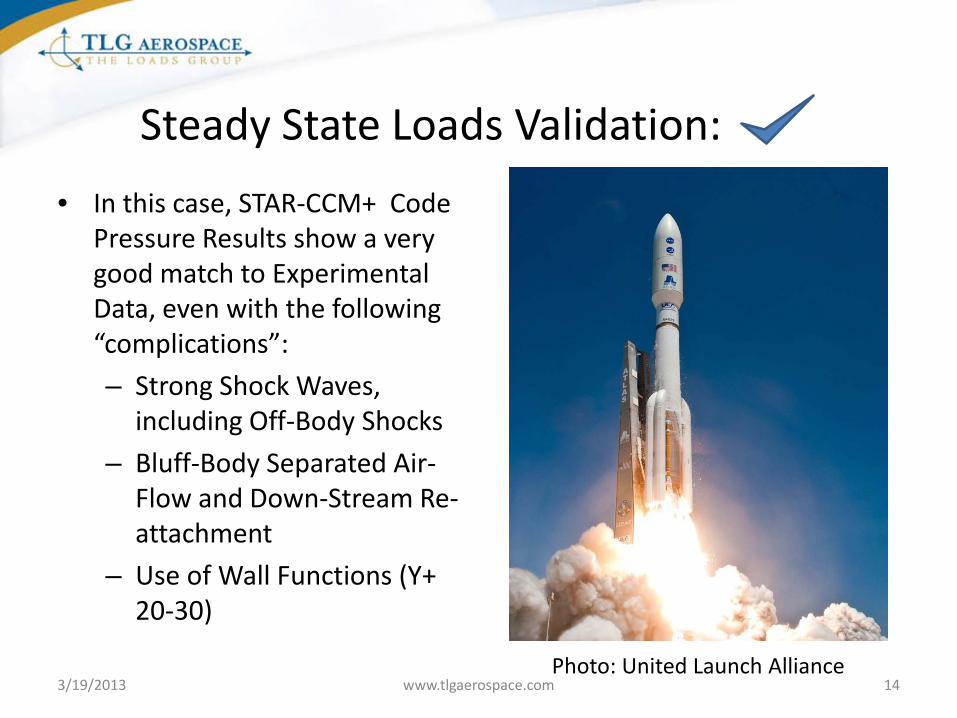
Steady State Loads Validation:

• In this case, STAR-CCM+ Code Pressure Results show a very good match to Experimental Data, even with the following “complications”:

– Strong Shock Waves, including Off-Body Shocks

– Bluff-Body Separated Air-Flow and Down-Stream Re-attachment

– Use of Wall Functions (Y+ 20-30)

Photo: United Launch Alliance 3/19/2013 www.tlgaerospace.com 14

Unsteady Pressure Validation

• Well the Steady-State Solution was easy!

• Moving along to Unsteady Buffet Loads Validation.

• NASA Tech. Memo.-X 778 has ΔCP(RMS) Data at numerous Mach no. and Alpha combinations, as well as frequency response info.

• Initial solution attempts were made with URANS: this was NOT the right approach!


Detached Eddy Simulation: Getting Started

• The best place to go for DES information is the source: Philippe Spalart

• Compared to a RANS solution we need to completely re-examine: – The minimum mesh size

– Time Step

– “Convergence Criteria”


Mesh Requirements for DES: Refinement in the Separation Zone

• Switched from Poly to TRIM for uniform cell size enforcement • Prism Layers increased to 18 with a first layer thickness of

.00275mm for a Wall Y+ between 0.5 and 1.0 • Volume Source for Refinement in the separation zone • Booster truncated to save mesh • Re-Meshed Surface is now 1.13M cells (was 165,000)


Determining the DES Region Required Cell Size

• STAR-CCM+ Unsteady Aero presentation used for guidance

• With the k-ω DES Implementation, we define 2 field functions:

• “Turbulent Length Scale” defined as:

• “Length Ratio”:

Turbulent Length Scale from a steady (RANS) solution 3/19/2013 www.tlgaerospace.com 18

DES Cell Size Cont.

• Goal: Turbulent Length Scale > 1 from a steady-state solution starting point

• Result: Minimum Cell Size in the DES region is 9mm • Size of the DES region limited by resources; for the cloud run

the 9mm region is extended aft and up

At times Rule Number 1 of DES appears to be: "Any unsatisfactory result reported to the author is due to the user‘s failure to run on a fine enough grid“ – Philippe Spalart 3/19/2013 www.tlgaerospace.com 19

DES Time Step Considerations: • Needs to be short enough to resolve the turbulent length scale

• Spalart guidance:

• For the M 0.81 run, Umax ≈ 300m/sec, and Δ0 = 0.009m

• Resulting time step: 30μs

Vorticity Iso-Surfaces Shed From the Payload Fairing


Key Flow Properties to Target for Validation

• Magnitude of the CP fluctuations in the separated region

• Location of flow re-attachment

• Frequency Content of the CP oscillations

Image Credit: ONERA, 2007


Now we have a Grid and Time Step; How Long (Physical Time) Do we Run?

• There are several “stopping criteria” 1. Reaching a “quasi-

steady” unsteady state

2. Mean of the Unsteady Pressures approaches the steady RANS solution

3. Sufficient time to resolve all frequencies of interest (at least 0.5 seconds for lower frequencies)

4. Until you run out of $$$$

Mean CP comparison, Unsteady Vs. RANS at 0.09 seconds real time simulated - closer than expected, but definitely not long enough (criteria 4 was used)


Putting it All Together: Running on “The Cloud”

• Final Mesh size: 39.75M cells • Initial steady-state solution run to 800

iterations • Unsteady Time step 30μs • 128 cores at R Systems • Elapsed Time/iteration = 8s • Very Limited budget (stopping criteria

#4); Only able to run 0.09s of real time – 25,000 iterations – 2.584e+7 accumulated CPU seconds


Development of the Unsteady Vorticity Field with Time

Initial State from Steady Solution Vorticity at 0.09s of “real time”

Well, it LOOKS nice, but how about the numbers?


Analysis for Loads: Pressures and Forces • Time Dependent Pressures at Discrete Points

• Darker lines are at Peak RMS location

• Lighter lines are in the Fully Separated Region


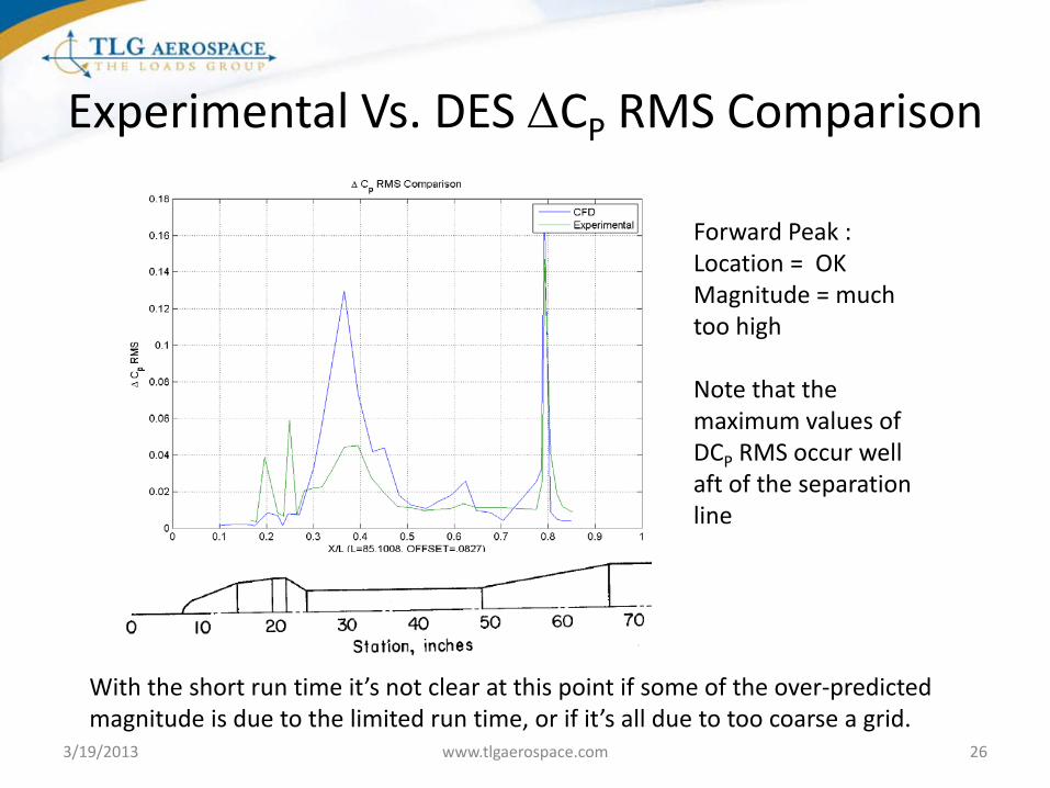
Experimental Vs. DES ∆CP RMS Comparison

Forward Peak : Location = OK Magnitude = much too high Note that the maximum values of DCP RMS occur well aft of the separation line

With the short run time it’s not clear at this point if some of the over-predicted magnitude is due to the limited run time, or if it’s all due to too coarse a grid.


Integrated Forces on Inter-Stage Sections: CX, CY and CZ

1 2 3 4


Frequency Content of Buffet Loads on Inter-Stage section 2

Power Spectral Density plotted log-log for CX, CY and CZ

Note: because of the short run time, frequencies < 30 Hz can’t be resolved


Re-Attachment Location • Expected results from

a range of experimental data: flow re-attachment should be about 3 step-heights aft of the separation point.

• The step is about 0.55m high; re-attachment from surface skin friction appears to be more like 5∆h downstream.

∆h

3∆h


Velocity Flow Visualization Movie • The movie starts at 0.038 s “real time” and with 30μs time steps • This was during development with the smaller mesh (23M cells);

a middle section runs at 100μs time steps • Total simulated time is just over 0.2 seconds • There are no cool movies from the cloud because I neglected to

ask for a head node with a full graphics card.


Pressure Variation with Time • Continuous Centerline Pressures from vertical (green)

and horizontal (red) cut planes

• Black squares are the experimental steady state values

• Location of the maximum ΔCP RMS is visually obvious


Conclusions on CFD Validation


• Steady State Pressures compare very well to experimental data, transonic and supersonic

• DES Solution truncated due to budget, but initial conclusions are:

• Magnitude of RMS DCP is too high; in other research this has indicated too coarse a mesh size • Re-Attachment Location 50% too far aft; the author has had this problem with RANS as well • Mean CP value in DES corresponds well to RANS • Frequency Content “looks reasonable”

The DES solver is clearly resolving the physics of a highly separated and turbulent flow field; but accurate forces (buffet) most likely require more mesh (Yes of course, more mesh – P. Spalart)

Computational Needs • The model run for the customer had 80M cells and ran on 128 cores at R Systems.

For 0.1 seconds of simulated time the computational time costs were: o 22,000 CPU hours

o Wall Clock time of 172 hrs (7.1 days)

• A good “minimum” run in order to allow the flow to stabilize and then capture sufficient data for low frequency resolutions is > 0.6s

• Wall clock time could be reduced by up to 6x by increasing the number of cores, but parallel losses will increase the CPU total cost

• Hypothetically then, a single flight analysis condition would require: o ≈200,000 CPU hours

o Wall clock still about 1 week


Future Computational Costs: Will the Wind Tunnel Replace the Computer?

• Wind Tunnel Economics: – Tunnel test preparation is 3-4 months (model

design + build) – A highly instrumented model costs $300k -

$450k – A pressurized transonic facility runs around

$5000/hour – When the wind is on, 1 second of “real time”

costs..... 1 second of real time! – Thousands of data points collected in 1

calendar week • Total Costs and Results:

– 3-4 Months – Around $1M for a good test – Thousands of data points (and no mesh

dependency study required!)

• Computational Data Acquisition Campaign • Optimistically assume the current 80M cell

model is sufficient • Assuming a $$/core/hour order of $0.10-0.20 • Each “Flight Condition” (i.e. single Mach and

Flow Angle) costs: – 1 Calendar Week – $20k in CPU + CFD License Costs

• For the same $1M as tunnel: – 50-100 data points depending on CPU costs – Serial Wall time: 50 weeks; or, with 4

concurrent simulations, 4 months

Vs


Questions?


Photo: United Launch Alliance

Everyone trusts the results of a test – except the person who ran the test

No one trusts the results of a computation – except the person who made it

detached eddy simulation analysis of a transonic rocket...

Documents