DETECTING AND CHARACTERIZING MALICIOUS WEBSITES

APPROVED BY SUPERVISING COMMITTEE:

Shouhuai Xu, Ph.D., Chair

Tom Bylander, Ph.D.

Hugh B. Maynard, Ph.D.

Ravi Sandhu, Ph.D.

Maochao Xu, Ph.D.

Accepted:Dean, Graduate School

Copyright 2014 Li XuAll rights reserved.

DEDICATION

I dedicate my dissertation work to my wife Yang Juan and lovely son Xu Ding. A special feeling

of gratitude to my loving parents, Xu Zuguo and Zheng Qiufen whose support during years of

graduate work was essential. I also dedicate this dissertation to my sister Wan Xuan, brother-in-

law Yang Shaoxiong and my parents-in-law who have never left my side.

DETECTING AND CHARACTERIZING MALICIOUS WEBSITES

by

LI XU, MS. C.

DISSERTATIONPresented to the Graduate Faculty of

The University of Texas at San AntonioIn Partial FulfillmentOf the Requirements

For the Degree of

DOCTOR OF PHILOSOPHY IN COMPUTER SCIENCE

THE UNIVERSITY OF TEXAS AT SAN ANTONIOCollege of Science

Department of Computer ScienceAugust 2014

All rights reserved

INFORMATION TO ALL USERSThe quality of this reproduction is dependent upon the quality of the copy submitted.

In the unlikely event that the author did not send a complete manuscriptand there are missing pages, these will be noted. Also, if material had to be removed,

a note will indicate the deletion.

Microform Edition © ProQuest LLC.All rights reserved. This work is protected against

unauthorized copying under Title 17, United States Code

ProQuest LLC.789 East Eisenhower Parkway

P.O. Box 1346Ann Arbor, MI 48106 - 1346

UMI 3637094Published by ProQuest LLC (2014). Copyright in the Dissertation held by the Author.

UMI Number: 3637094

ACKNOWLEDGEMENTS

This dissertation would never have been completed without the help and support of Dr. Shouhuai

Xu, my supervisor, who advised me and worked with me. My friends Zhenxin Zhan, Qingji Zheng

and Weiliang Luo were also an invaluable helps many times. I also would like to thank my com-

mittee members: Dr. Tom Bylander, Dr. Hugh Maynard Dr. Ravi Sandhu, and Dr. Maochao

Xu.

The research described in the dissertation was partly supported by Prof. Shouhuai Xu’s ARO

Grant # W911NF-12-1-0286 and AFOSR Grant # FA9550-09-1-0165. The studies were approved

by IRB.

August 2014

iv

DETECTING AND CHARACTERIZING MALICIOUS WEBSITES

Li Xu, Ph.D.The University of Texas at San Antonio, 2014

Supervising Professor: Shouhuai Xu, Ph.D.

Malicious websites have become a big cyber threat. Given that malicious websites are in-

evitable, we need good solutions for detecting them. The present dissertation makes three con-

tributions that are centered on addressing the malicious websites problem. First, it presents a

novel cross-layer method for detecting malicious websites, which essentially exploits the network-

layer "lens" to expose more information about malicious websites. Evaluation based on some real

data shows that cross-layer detection is about 50 times faster than the dynamic approach, while

achieving almost the same detection effectiveness (in terms of accuracy, false-negative rate, and

false-positive rate). Second, it presents a novel proactive detection method to deal with adaptive

attacks that can be exploited to evade the static detection approach. By formulating a novel security

model, it characterizes when proactive detection can achieve significant success against adaptive

attacks. Third, it presents statistical characteristics on the evolution of malicious websites. The

characteristics offer deeper understanding about the threat of malicious websites.

v

TABLE OF CONTENTS

Acknowledgements . . . . . . . . . . . . . . . . . . . . . . . . . . . . . . . . . . . . . . iv

Abstract . . . . . . . . . . . . . . . . . . . . . . . . . . . . . . . . . . . . . . . . . . . . . v

List of Tables . . . . . . . . . . . . . . . . . . . . . . . . . . . . . . . . . . . . . . . . . . ix

List of Figures . . . . . . . . . . . . . . . . . . . . . . . . . . . . . . . . . . . . . . . . . xi

Chapter 1: Introduction . . . . . . . . . . . . . . . . . . . . . . . . . . . . . . . . . . . . 1

1.1 Problem Statement and Research Motivation . . . . . . . . . . . . . . . . . . . . . 1

1.2 Dissertation Contributions . . . . . . . . . . . . . . . . . . . . . . . . . . . . . . 3

Chapter 2: Data Collection, Pre-Processing and Feature Definitions . . . . . . . . . . . 4

2.1 Data Collection . . . . . . . . . . . . . . . . . . . . . . . . . . . . . . . . . . . . 4

2.2 Data Pre-Processing . . . . . . . . . . . . . . . . . . . . . . . . . . . . . . . . . . 6

2.3 Data Description . . . . . . . . . . . . . . . . . . . . . . . . . . . . . . . . . . . 7

2.3.1 Application-Layer Features . . . . . . . . . . . . . . . . . . . . . . . . . 7

2.3.2 Network-Layer Features . . . . . . . . . . . . . . . . . . . . . . . . . . . 10

2.4 Effectiveness Metrics . . . . . . . . . . . . . . . . . . . . . . . . . . . . . . . . . 14

Chapter 3: Cross-layer Detection of Malicious Websites . . . . . . . . . . . . . . . . . . 15

3.1 Introduction . . . . . . . . . . . . . . . . . . . . . . . . . . . . . . . . . . . . . . 15

3.2 Single-Layer Detection of Malicious Websites . . . . . . . . . . . . . . . . . . . . 17

3.3 Cross-Layer Detection of Malicious Website . . . . . . . . . . . . . . . . . . . . . 19

3.3.1 Overall Effectiveness of Cross-Layer Detection . . . . . . . . . . . . . . . 20

3.3.2 Which Features Are Indicative? . . . . . . . . . . . . . . . . . . . . . . . 23

3.3.3 How Did the Network Layer Help Out? . . . . . . . . . . . . . . . . . . . 26

vi

3.3.4 Performance Evaluation . . . . . . . . . . . . . . . . . . . . . . . . . . . 29

3.3.5 Deployment . . . . . . . . . . . . . . . . . . . . . . . . . . . . . . . . . . 32

3.4 Related Work . . . . . . . . . . . . . . . . . . . . . . . . . . . . . . . . . . . . . 34

3.5 Summery . . . . . . . . . . . . . . . . . . . . . . . . . . . . . . . . . . . . . . . 35

Chapter 4: Proactive Detection of Adaptive Malicious Websites . . . . . . . . . . . . . . 37

4.1 Introduction . . . . . . . . . . . . . . . . . . . . . . . . . . . . . . . . . . . . . . 37

4.2 Adaptive Attacks and Their Power . . . . . . . . . . . . . . . . . . . . . . . . . . 39

4.2.1 Adaptive Attack Model and Algorithm . . . . . . . . . . . . . . . . . . . 39

4.2.2 Power of Adaptive Attacks . . . . . . . . . . . . . . . . . . . . . . . . . . 53

4.3 Proactive Defense against Adaptive Attacks . . . . . . . . . . . . . . . . . . . . . 57

4.3.1 Proactive Defense Model and Algorithm . . . . . . . . . . . . . . . . . . . 57

4.3.2 Evaluation and Results . . . . . . . . . . . . . . . . . . . . . . . . . . . . 59

4.4 Related Work . . . . . . . . . . . . . . . . . . . . . . . . . . . . . . . . . . . . . 63

4.5 Summary . . . . . . . . . . . . . . . . . . . . . . . . . . . . . . . . . . . . . . . 64

Chapter 5: Characterizing and Detecting Evolving Malicious Websites . . . . . . . . . 66

5.1 Introduction . . . . . . . . . . . . . . . . . . . . . . . . . . . . . . . . . . . . . . 66

5.2 Our Contributions . . . . . . . . . . . . . . . . . . . . . . . . . . . . . . . . . . . 66

5.3 Data Description . . . . . . . . . . . . . . . . . . . . . . . . . . . . . . . . . . . 67

5.4 On the Evolution of Malicious Websites . . . . . . . . . . . . . . . . . . . . . . . 67

5.4.1 Analysis Methodology . . . . . . . . . . . . . . . . . . . . . . . . . . . . 67

5.4.2 Characteristics of the Evolving Websites . . . . . . . . . . . . . . . . . . . 68

5.5 Online Learning . . . . . . . . . . . . . . . . . . . . . . . . . . . . . . . . . . . . 70

5.6 Related Work . . . . . . . . . . . . . . . . . . . . . . . . . . . . . . . . . . . . . 71

5.7 Summery . . . . . . . . . . . . . . . . . . . . . . . . . . . . . . . . . . . . . . . 72

Chapter 6: Conclusion and Future Work . . . . . . . . . . . . . . . . . . . . . . . . . . 73

vii

Bibliography . . . . . . . . . . . . . . . . . . . . . . . . . . . . . . . . . . . . . . . . . . 74

Vita

viii

LIST OF TABLES

Table 3.1 Single-layer average effectiveness (Acc: detection accuracy; FN: false neg-

ative rate; FP: false positive rate) . . . . . . . . . . . . . . . . . . . . . . . 18

Table 3.2 Cross-layer average effectiveness (Acc: detection accuracy; FN: false-negative

rate; FP: false-positive rate). In the XOR-aggregation cross-layer detection,

the portions of websites queried in the dynamic approach (i.e., the websites

for which the application-layer and cross-layer detection models have dif-

ferent opinions) with respect to the four machine learning algorithms are

respectively: without using feature selection, (19.139%, 1.49%, 1.814%,

0.014%); using PCA feature selection, (17.448%, 1.897%, 3.948%, 0.307%);

using Subset feature selection, (8.01%, 2.725%, 3.246%, 0.654%); using

InfoGain feature section, (13.197%, 2.86%, 4.178%, 0.37%). There-

fore, J48 classifier is appropriate for XOR-aggregation. . . . . . . . . . . . 21

Table 3.3 Breakdown of the average mis-classifications that were corrected by the

network-layer classifiers, where N/A means that the network-layer cannot

help (see text for explanation). . . . . . . . . . . . . . . . . . . . . . . . . 26

Table 3.4 Measured performance comparison between the data-aggregation cross-

layer J48 classifier and the dynamic approach (the Capture-HPC client hon-

eypot) with 3,062 input URLs (1,562 malicious URLs + 1,500 Benign URLs) 31

Table 4.1 Experiment results with M0(D1) in terms of average false-negative rate

(FN), average number of manipulated features (Number_of_MF), average

percentage of failed attempts (FA), where “average" is over the 40 days of

the dataset mentioned above. . . . . . . . . . . . . . . . . . . . . . . . . . 54

ix

Table 4.2 Experiment results of M0(D1) by treating as non-manipulatable the InfoGain-

selected five application-layer features and four network-layer features.

Metrics are as in Table 4.1. . . . . . . . . . . . . . . . . . . . . . . . . . . 56

Table 4.3 Experiment results of M0(D1) by treating the features that were manip-

ulated by adaptive attack AA as non-manipulatable. Notations are as in

Tables 4.1-4.2. . . . . . . . . . . . . . . . . . . . . . . . . . . . . . . . . . 56

Table 4.4 Data-aggregation cross-layer proactive detection with STA = STD. For

baseline case M0(D0), ACC = 99.68%, true-positive rate TP =99.21%,

false-negative rate FN=0.79%, and false-positive rate FP=0.14%. . . . . . 61

Table 4.5 Data-aggregation cross-layer proactive detection against adaptive attacks

with FD = FA. . . . . . . . . . . . . . . . . . . . . . . . . . . . . . . . . . 61

x

LIST OF FIGURES

Figure 2.1 Data collection system architecture. . . . . . . . . . . . . . . . . . . . . . 5

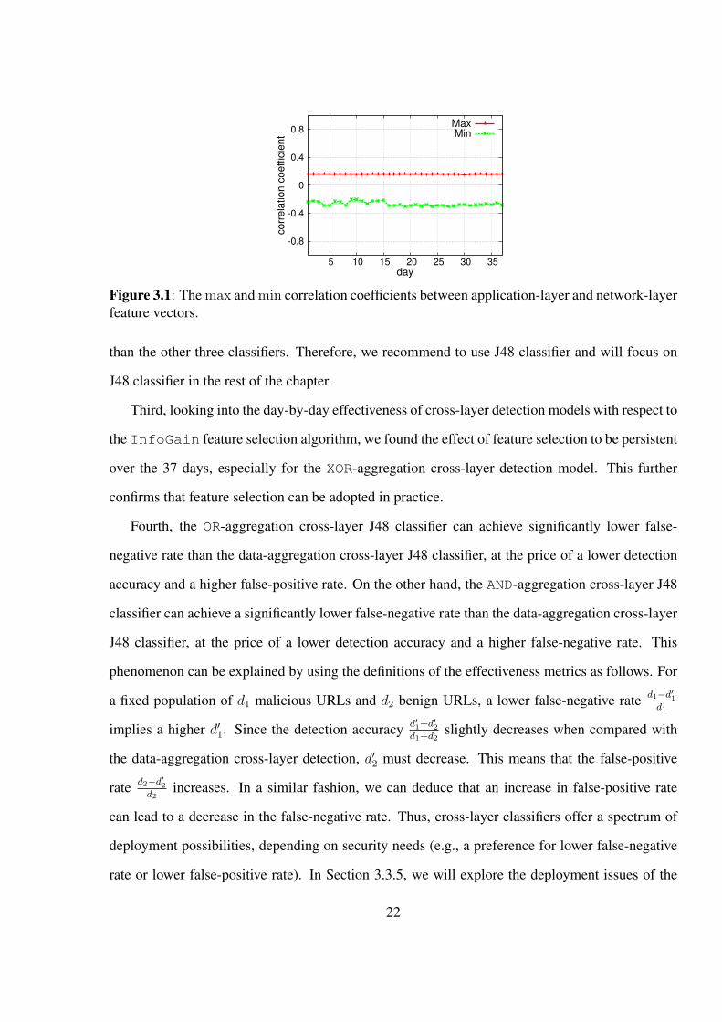
Figure 3.1 The max and min correlation coefficients between application-layer and

network-layer feature vectors. . . . . . . . . . . . . . . . . . . . . . . . . 22

Figure 3.2 Portions of the application-layer and network-layer classifiers correspond-

ing to the two URLs. . . . . . . . . . . . . . . . . . . . . . . . . . . . . . 27

Figure 3.3 Example deployment of the cross-layer detection system as the front-end

of a bigger solution because XOR-aggregation J48 classifiers achieve ex-

tremely high detection accuracy, extremely low false-negative and false-

positive rates. . . . . . . . . . . . . . . . . . . . . . . . . . . . . . . . . . 33

Figure 4.1 Adaptive attack algorithm AA(MLA,M0, D0, ST,C, F, α), where MLA is

the defender’s machine learning algorithm, D′0 is the defender’s training

data, M0 is the defender’s detection scheme that is learned from D′0 by us-

ing MLA, D0 is the feature vectors that are examined by M0 in the absence

of adaptive attacks, ST is the attacker’s adaptation strategy, C is a set of

manipulation constraints, F is the attacker’s (deterministic or randomized)

manipulation algorithm that maintains the set of constraints C, α is the

number of rounds the attacker runs its manipulation algorithms. Dα is the

manipulated version of D0 with malicious feature vectors D0.malicious

manipulated. The attacker’s objective is make M0(Dα) have high false-

negative rate. . . . . . . . . . . . . . . . . . . . . . . . . . . . . . . . . . 41

Figure 4.2 Example J48 classifier and feature manipulation. For inner node v10 on the

benign_path ending at benign_leaf v3, we have v10.feature = “X4” and

v10.feature.value = X4.value. . . . . . . . . . . . . . . . . . . . . . . . 49

xi

Figure 4.3 Impact of defender’s proactiveness γ vs. attacker’s adaptiveness α on de-

tection accuracy (average over the 40 days) under various “STD × STA”

combinations, where α ∈ [0, 8], γ ∈ [0, 9], PAR, SEQ and FULL respectively

stand for paraleel, sequential and full adaptation strategy, “SEQ vs.

APR" means STD = sequential and STA = parallel etc. . . . . . . . . 62

Figure 5.1 Detection accuracy of Mi(Dj) using the random forest method, where x-

axis represents day i (from which model Mi is learned) and y-axis repre-

sents detection accuracy. . . . . . . . . . . . . . . . . . . . . . . . . . . . 69

Figure 5.2 Detection accuracy of Mi(Dj) using the adaboost method, where x-axis

represents day i (from which model Mi is learned) and y-axis represents

detection accuracy. . . . . . . . . . . . . . . . . . . . . . . . . . . . . . . 69

Figure 5.3 Detection accuracy of random forest classification models obtained by us-

ing online learning algorithm LRsgd with non-adaptive or adpative strat-

egy, where x-axis represents j, y-axis represents the detection accuracy

rate, M1..j(Dj) means that the model M1..j is learned from the entire his-

tory of training data from D1, . . . , Dj (non-adaptive strategy), and Mi..j

means that the model Mi..j is learned from partial history of trainig data

from Di, . . . , Dj (adaptive strategy). . . . . . . . . . . . . . . . . . . . . . 71

xii

Chapter 1: INTRODUCTION

1.1 Problem Statement and Research Motivation

Today, many client-side attackers are part of organized crime with the intent to defraud their vic-

tims. Their goal is to deploy malware on a victim’s machine and to start collecting sensitive data,

such as online account credentials and credit card numbers. Since attackers have a tendency to take

the path of least resistance and many traditional attack paths are barred by a basic set of security

measures, such as firewalls or anti-virus engines, the “black hats" are turning to easier, unprotected

attack paths to place their malware onto the end user’s machine. They are turning to client-side

attacks, because they can cause the automatic download and execution of malware in browsers,

and thus compromise vulnerable computers [50]. The phenomenon of malicious websites will

persevere at least in the foreseeable future because we cannot prevent websites from being com-

promised or abused. Existing approaches to detecting malicious websites can be classified into two

categories:

• The static approach aims to detect malicious websites by analyzing their URLs [39, 40] or

their contents [61]. This approach is very efficient and thus can scale up to deal with the

huge population of websites in cyberspace. This approach however has trouble coping with

sophisticated attacks that include obfuscation [54], and thus can cause high false-negative

rates by classifying malicious websites as benign ones.

• The dynamic approach aims to detect malicious websites by analyzing their run-time behav-

ior using Client Honeypots or their like [4, 5, 42, 58, 63]. Assuming the underlying detection

is competent, this approach is very effective. This approach however, is inefficient because

it runs or emulates the browser and possibly the operating system [14]. As a consequence,

this approach cannot scale up to deal with the large number of websites in cyberspace.

Because of the above, it has been advocated to use a front-end light-weight tool, which is

mainly based on static analysis and aims to rapidly detect suspicious websites, and a back-end more

1

powerful but much slower tool (e.g., dynamic analysis or even binary analysis), which conducts

a deeper analysis of the detected suspicious websites. While conceptually attractive, the success

of this hybrid approach fundamentally relies on the assumption that the front-end static analysis

does have very low false-negative rates; otherwise, many malicious websites will not be detected

even if the back-end dynamic analysis tools are powerful. However, this assumption can be easily

violated because of the following.

First, in real life, the attacker could defeat pure static analysis by exploiting various sophisti-

cated techniques such as obfuscation and redirection. Redirection technique was originally intro-

duced for the purpose of making various changes to the web servers transparent to their users. Not

surprisingly, this technique has also been abused to launch cyber attacks. Assuming the back-end

detection tool is effective, the false-negative rate of the front-end static analysis tool determines

the detection power (resp. scalability) of the hybrid approach. Therefore, in order to achieve

high detection accuracy and high scalability simultaneously, the hybrid solution must have mini-

mum false-negatives and false-positives. This requirement is necessary to achieve the best of both

worlds — static analysis and dynamic analysis.

Second, the attacker can get the same data and therefore use the same machine learning al-

gorithms to derive the defender’s classifiers. This is plausible because in view of Kerckhoffs’s

Principle in cryptography, we should assume that the defender’s learning algorithms are known

to the attacker. As a consequence, the attacker can always act one step ahead of the defender by

adjusting its activities so as to evade detection.

The above two issues lead to the following question: how can we achieve the best of both

static and dynamic analysis, and go beyond? This question is clearly important and motivates the

investigation presented in this dissertation. For solutions based on a hybrid architecture to succeed,

a key factor is to reduce both false-positives and false-negatives of the static analysis tools. While

intuitive, this crucial aspect has not been thoroughly investigated and characterized in the literature.

This dissertation aims to take a substantial step towards the ultimate goal.

2

1.2 Dissertation Contributions

The first contribution is a novel cross-layer malicious website detection approach which analyzes

network-layer traffic and application-layer website contents simultaneously. Existing malicious

website detection approaches have technical and computational limitations in detecting sophisti-

cated attacks and analyzing massive data. The main objective of our research is to minimize these

limitations of malicious website detection. Detailed data collection and performance evaluation

methods are also presented. Evaluations based on data collected during 37 days show that the

computing time of the cross-layer detection is 50 times faster than the dynamic approach while

detection can be almost as effective as the dynamic approach. Experimental results indicate that

the cross-layer detection outperforms existing malicious website detection techniques.

The second contribution addresses the following question: What if the attacker is adaptive? We

present three adaptation strategies that may be used by the attacker to launch adaptive attacks, and

can be exploited by the defender to launch adaptive defense. We also provide two manipulation

algorithms that attempt to bypass the trained J48 detection system. The algorithms demonstrate

how easy it can be for an adaptive attacker to evade non-adaptive detection. We show how our

defense algorithms can effectively deal with adaptive attacks, and thus make our detection system

resilient to adaptive attacks. We characterize the effectiveness of proactive defense against adaptive

attacks. We believe that this investigation opens the door for an interesting research direction.

The third contribution is the investigation of the “natural” evolution of malicious websites. We

present characteristics of the evolution, which can be exploited to design future defense systems

against malicious websites.

3

Chapter 2: DATA COLLECTION, PRE-PROCESSING AND FEATURE

DEFINITIONS

We now describe the methodology underlying our study, including data collection, data pre-process-

ing, evaluation metrics and data analysis methods. The methodology is general enough to accom-

modate single-layer analyses, but will be extended slightly to accommodate extra ideas that are

specific to cross-layer analyses.

2.1 Data Collection

In order to facilitate cross-layer analysis and detection, we need an automated system to collect

both the application-layer website contents and the corresponding network-layer traffic. The ar-

chitecture of our automated data collection system is depicted in Figure 2.1. At a high level, the

data collection system is centered on a crawler. The crawler takes a list of URLs as input, automat-

ically fetches the website contents by launching HTTP requests and tracks the redirects that are

identified from the website contents (elaborated below). The crawler also uses the URLs, includ-

ing the input URL and the detected redirection URLs, to query the DNS, Whois, and Geographic

services. This collects information about the registration dates of websites and the geographic

locations of the URL owners/registrants. The application-layer website contents and the corre-

sponding network-layer IP packets are recorded separately (where the IP packets are caused by

application-layer activities), but are indexed by the input URLs to facilitate cross-layer analysis.

As mentioned above, the data collection system proactively tracks redirects by analyzing the

website contents in a static fashion. Specifically, it considers the following four types of redi-

rects. The first type is the server side redirects, which are initiated either by server rules (i.e.,

.htaccess file) or by server side page code such as PHP. These redirects often utilize HTTP

300 level status codes. The second type is JavaScript-based redirects. The third type is the refresh

Meta tag and the HTTP refresh header, which allow the URLs of the redirection pages to be speci-

fied. The fourth type is the embedded file redirects. Some examples of this type are the following:

4

Figure 2.1: Data collection system architecture.

<script src=’badsite.php’> </script>, <iframe src=’badsite.php’/>,

and <img src=’badsite.php’/>.

The input URLs may consist of malicious and benign websites. A URL is malicious if the cor-

responding website content is malicious or any of its redirects leads to a URL that corresponds to

malicious content; otherwise, it is benign. In this chapter, the terms malicious URLs and malicious

websites are used interchangeably. In our experimental system for training and testing detection

models, malicious URLs are initially obtained from the following blacklists: compuweb.com/

url-domain-bl.txt, malware.com.br, malwaredomainlist.com, zeustracker.

abuse.ch and spyeyetracker.abuse.ch. Since some of the blacklisted URLs are not ac-

cessible or malicious any more, we use the high-interactive client honeypot called Capture-HPC

version 3.0 [58] to identify the subset of URLs that are still accessible and malicious. We empha-

size that our experiments were based on Capture-HPC, which is assumed to offer the ground truth.

This is a practical choice because we cannot manually analyze the large number of websites. Even

if we could, manual analysis might still be error-prone. Note that any dynamic analysis system

(e.g., another client honeypot system) can be used instead in a plug-and-play fashion. Pursuing a

client honeypot that truly offers the ground truth is an orthogonal research problem. The benign

5

URLs are obtained from alexa.com, which lists the top 2,088 websites that are supposed to be

well protected. The data was collected for a period of 37 days between 12/07/2011 and 01/12/2012,

with the input URLs updated daily.

2.2 Data Pre-Processing

Each input URL has an associated application-layer raw feature vector. The features record infor-

mation such as HTTP header fields, information returned by DNS, Whois and Geographic services,

information about JavaScript functions that are called in the JavaScript code embedded into the

website content, and information about redirects (e.g., redirection method, whether or not a redirect

points to a different domain, and the number of redirection hops). Since different URLs may lead

to different numbers of redirection hops, the raw feature vectors may not have the same number

of features. In order to facilitate analysis, we use a pre-processing step to aggregate multiple-hop

information into some artificial single-hop information. Specifically, for numerical data, we ag-

gregate them by using their average instead; for boolean data, we aggregate them by taking the OR

operation; for nominal data, we only consider the final destination URL of the redirection chain.

For example, suppose the features of interest are: (Content-Length, “Does JavaScript func-

tion eval() exist in the code?", Country). Suppose an input URL is redirected twice to reach

the final destination URL, and the raw feature vectors corresponding to the input, first redirect,

and second redirect URLs are (100, FALSE, US), (200, FALSE, UK), and (300, TRUE, RUSSIA),

respectively. We aggregate the three raw features into a single feature (200, TRUE, RUSSIA). Af-

ter the pre-processing step, the application-layer data have 105 features, some of which will be

elaborated below.

Each input URL has an associated network-layer raw feature vector. The features are extracted

from the corresponding PCAP (Packet CAPture) files that are recorded when the crawler accesses

the URLs. There are 19 network-layer features that are derived from the IP, UDP/TCP or flow

level, where a flow is uniquely identified by a tuple (source IP, source port number, destination IP,

destination port number, protocol).

6

Each URL is also associated with a cross-layer feature vector, which is simply the concatena-

tion of its associated application-layer and network-layer feature vectors.

2.3 Data Description

The resulting data has 105 application-layer features of 4 sub-classes and 19 network-layer features

of 3 sub-classes. Throughout the chapter, “average" means the average over the 37-day data.

2.3.1 Application-Layer Features

Feature based on the URL lexical information We defined 15 features based on the URL

lexical information, 3 of which are elaborated below.

(A1): URL_Length. URLs include the following parts: protocol, domain name or plain IP ad-

dress, optional port, directory file. When using HTTP Get to request information from a server,

there will be an additional part consisting of a question mark followed by a list of “key = value"

pairs. In order to make malicious URLs hard to blacklist, malicious URLs often include automati-

cally and dynamically generated long random character strings. Our data showed that the average

length of benign URLs is 18.23 characters, whereas the average length of malicious URLs is 25.11

characters.

(A2): Number_of_special_characters_in_URL. This is the number of special charac-

ters (e.g., ?, -, _, =, %) that appear in a URL. Our data showed that benign URLs used on average

2.93 special characters, whereas malicious URLs used on average 3.36 special characters.

(A3): Presence_of_IP_address_in_URL. This feature indicates whether an IP address

is presented as the domain name in a URL. Some websites use IP addresses instead of domain

names in the URL because the IP addresses represent the compromised computers that actually do

not have registered domain names. This explains why this feature may be indicative of malicious

URLs. This feature has been used in [14].

7

Features based on the HTTP header information We defined 15 features based on the HTTP

header information, 4 of which are elaborated below.

(A4): Charset. This is the encoding charset of the URL in question (e.g., iso-8859-1). It hints

at the language a website uses and the ethnicity of the targeted users of the website. It is also

indicative of the nationality of the webpage.

(A5): Server. This is the server field in the http response head. It gives the software information

at the server side, such as the webserver type/name and its version. Our data showed that the Top

3 webservers that were abused to host malicious websites are Apache, Microsoft IIS, and nginx,

which respectively correspond to 322, 97, and 44 malicious websites on average. On the other

hand, Apache, Microsoft IIS, and nginx were abused to host 879, 253, and 357 benign websites on

average.

(A6): Cache_control. Four cache control strategies are identified in the websites of our data:

no-cache, private, public, and cache with max-age. The average numbers of benign websites that

use these strategies are respectively 444, 276, 67, and 397, whereas the average numbers of mali-

cious websites that use these strategies are respectively 99, 46, 0.5, and 23.

(A7): Content_length. This feature indicates the content-length field of a HTTP header. For

malicious URLs, the value of this field may be manipulated so that it does not match the actual

length of the content.

Features based on the host information (include DNS, Whois data) We defined 7 features

based on the host information, 5 of which are elaborated below.

(A8-A9): RegDate and Updated_date. These two features are closely related to each other.

They indicate the dates the webserver was registered and updated with the Whois service, respec-

tively. Our data showed that on average, malicious websites were registered in 2004, whereas

benign websites were registered in 2002. We also observed that on average, malicious websites

were updated in 2009, one year earlier than the average update date of 2010 for benign websites .

(A10-A11): Country and Stateprov. These two features respectively indicate the counter

8

and the location where the website was registered. These two features, together with the afore-

mentioned charset feature, can be indicative of the locations of websites. Our data showed that

the average numbers of benign websites registered in US, NL, and AU are respectively 618, 523,

and 302, whereas the average numbers of malicious websites registered in US, NL, and AU are

respectively 152, 177, and 98.

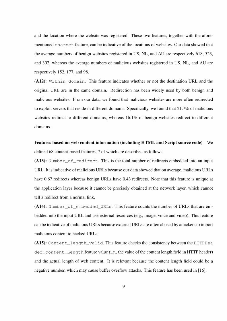
(A12): Within_domain. This feature indicates whether or not the destination URL and the

original URL are in the same domain. Redirection has been widely used by both benign and

malicious websites. From our data, we found that malicious websites are more often redirected

to exploit servers that reside in different domains. Specifically, we found that 21.7% of malicious

websites redirect to different domains, whereas 16.1% of benign websites redirect to different

domains.

Features based on web content information (including HTML and Script source code) We

defined 68 content-based features, 7 of which are described as follows.

(A13): Number_of_redirect. This is the total number of redirects embedded into an input

URL. It is indicative of malicious URLs because our data showed that on average, malicious URLs

have 0.67 redirects whereas benign URLs have 0.43 redirects. Note that this feature is unique at

the application layer because it cannot be precisely obtained at the network layer, which cannot

tell a redirect from a normal link.

(A14): Number_of_embedded_URLs. This feature counts the number of URLs that are em-

bedded into the input URL and use external resources (e.g., image, voice and video). This feature

can be indicative of malicious URLs because external URLs are often abused by attackers to import

malicious content to hacked URLs.

(A15): Content_length_valid. This feature checks the consistency between the HTTPHea

der_content_Length feature value (i.e., the value of the content length field in HTTP header)

and the actual length of web content. It is relevant because the content length field could be a

negative number, which may cause buffer overflow attacks. This feature has been used in [16].

9

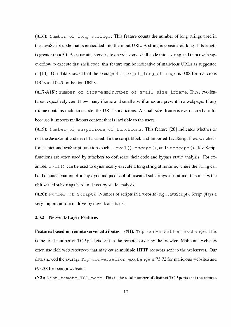
(A16): Number_of_long_strings. This feature counts the number of long strings used in

the JavaScript code that is embedded into the input URL. A string is considered long if its length

is greater than 50. Because attackers try to encode some shell code into a string and then use heap-

overflow to execute that shell code, this feature can be indicative of malicious URLs as suggested

in [14]. Our data showed that the average Number_of_long_strings is 0.88 for malicious

URLs and 0.43 for benign URLs.

(A17-A18): Number_of_iframe and number_of_small_size_iframe. These two fea-

tures respectively count how many iframe and small size iframes are present in a webpage. If any

iframe contains malicious code, the URL is malicious. A small size iframe is even more harmful

because it imports malicious content that is invisible to the users.

(A19): Number_of_suspicious_JS_functions. This feature [28] indicates whether or

not the JavaScript code is obfuscated. In the script block and imported JavaScript files, we check

for suspicious JavaScript functions such as eval(), escape(), and unescape(). JavaScript

functions are often used by attackers to obfuscate their code and bypass static analysis. For ex-

ample, eval() can be used to dynamically execute a long string at runtime, where the string can

be the concatenation of many dynamic pieces of obfuscated substrings at runtime; this makes the

obfuscated substrings hard to detect by static analysis.

(A20): Number_of_Scripts. Number of scripts in a website (e.g., JavaScript). Script plays a

very important role in drive-by download attack.

2.3.2 Network-Layer Features

Features based on remote server attributes (N1): Tcp_conversation_exchange. This

is the total number of TCP packets sent to the remote server by the crawler. Malicious websites

often use rich web resources that may cause multiple HTTP requests sent to the webserver. Our

data showed the average Tcp_conversation_exchange is 73.72 for malicious websites and

693.38 for benign websites.

(N2): Dist_remote_TCP_port. This is the total number of distinct TCP ports that the remote

10

webserver used during the conversation with the crawler. Our data showed that benign websites

often use the standard http port 80, whereas malicious websites often use some of the other ports.

Our data showed the average Dist_remote_TCP_port is 1.98 for malicious websites and 1.99

for benign websites.

(N3): Remote_ips. This is the number of distinct remote IP addresses connected by the crawler,

not including the DNS server IP addresses. Multiple remote IP addresses can be caused by redi-

rection, internal and external resources that are embedded into the webpage corresponding to the

input URL. Our data showed the average Remote_ips is 2.15 for malicious websites and 2.40

for benign websites.

Features based on crawler-server communication (N4): App_bytes. This is the number of

Bytes of the application-layer data sent by the crawler to the remote webserver, not including the

data sent to the DNS servers. Malicious URLs often cause the crawler to initiate multiple requests

to remote servers, such as multiple redirections, iframes, and external links to other domain names.

Our data showed the average App_bytes is 36818 bytes for malicious websites and 53959 bytes

for benign websites.

(N5): UDP_packets. This is the number of UDP packets generated during the entire lifecycle

when the crawler visits a URL, not including the DNS packets. Benign websites running an on-

line streaming application (such as video, audio and internet phone) will generate numerous UDP

packets, whereas malicious websites often exhibit numerous TCP packets. Our data showed the

average UDP_packets for both benign and malicious URLs are 0 because the crawler does not

download any video/audio stream from the sever.

(N6): TCP_urg_packets. This is the number of urgent TCP packets with the URG (urgent)

flag set. Some attacks abuse this flag to bypass the IDS or firewall systems that are not properly

set up. If a packet has the URGENT POINTER field set, but the URG flag is not set, this consti-

tutes a protocol anomaly and usually indicates a malicious activity that involves transmission of

malformed TCP/IP datagrams. Our data showed the average TCP_urg_packets is 0.0003 for

11

malicious websites and 0.001 for benign websites.

(N7): Source_app_packets. This is the number of packets send by the crawler to remote

servers. Our data showed the average source_app_packets is 130.65 for malicious websites

and 35.44 for benign websites.

(N8): Remote_app_packets. This is the number of packets sent by the remote webserver(s)

to the crawler. This feature is unique to the network layer. Our data showed the average value of

this feature is 100.47 for malicious websites and 38.28 for benign websites.

(N9): Source_app_bytes. This is the volume (in bytes) of the crawler-to-webserver commu-

nications. Our data showed that the average application payload volumes of benign websites and

malicious websites are about 146 bytes and 269 bytes, respectively.

(N10): Remote_app_bytes. This is the volume (in bytes) of data from the webserver(s) to the

crawler, which is similar to feature Source_app_byte. Our data showed the average value of

this feature is 36527 bytes for malicious websites and 49761 bytes for benign websites.

(N11): Duration. This is the the duration of time, starting from the point the crawler was

fed with an input URL to the point the webpage was successfully obtained by the crawler or an

error returned by the webserver. This feature is indicative of malicious websites because visiting

malicious URLs may cause the crawler to send multiple DNS queries and multiple connections to

multiple web servers, which could lead to a high volume of communications. Our data showed

that visiting benign websites caused 0.793 seconds duration time on average, whereas visiting

malicious websites caused 2.05 seconds duration time on average.

(N12): Avg_local_pkt_rate. This is the average rate of IP packets (packets per second)

that are sent from the crawler to the remote webserver(s) with respect to an input URL, which

equals source_app_packets/duration. This feature measures the packet sending speed

of the crawler, which is related to the richness of webpage resources. Webpages containing rich

resources often cause the crawler to send a large volume of data to the server. Our data showed the

average Avg_local_pkt_rate is 63.73 for malicious websites and 44.69 for benign websites.

(N13): Avg_remote_pkt_rate. This is the average IP packet rate (in packets per second) of

12

packets sent from the remote server to the crawler. When multiple remote IP addresses are in-

volved (e.g., because of redirection or because the webpage uses external links), we amortize the

number of packets, despite the fact that some remote IP addresses may send more packets than

others back to the crawler. Websites containing malicious code or contents can cause large vol-

ume communications between the remote server(s) and the crawler. Our data showed the average

Avg_remote_pkt_rate is 63.73 for malicious websites and is 48.27 for benign websites.

(N14): App_packets. This is the total number of IP packets generated for obtaining the con-

tent corresponding to an input URL, including redirects and DNS queries. It measures the data

exchange volume between the crawler and the remote webserver(s). Our data showed the average

value of this feature is 63.73 for malicious websites and 48.27 for benign websites.

Features based on crawler-DNS flows (N15): DNS_query_times. This is the number of

DNS queries sent by the crawler. Because of redirection, visiting malicious URLs often causes the

crawler to send multiple DNS queries and to connect multiple remote webservers. Our data showed

the average value of this feature is 13.30 for malicious websites and 7.36 for benign websites.

(N16): DNS_response_time. This is the response time of DNS servers. Benign URLs often

have longer lifetimes and their domain names are more likely cached at local DNS servers. As

a result, the average value of this feature may be shorter for benign URLs. Our data showed the

average value of this feature is 13.29 ms for malicious websites and is 7.36 ms for benign websites.

Features based on aggregated values (N17): Iat_flow. This is the accumulated inter-arrival

time between consecutive flows. Given two consecutive flows, the inter-arrival time is the dif-

ference between the timestamps of the first packet in each flow. Our data showed the average

Iat_flow is 1358.4 for malicious websites and 512.99 for benign websites.

(N18): Flow_number. This is the number of flows generated during the entire lifecycle for

the crawler to download the web content corresponding to an input URL, including the recursive

queries to DNS and recursive access to redirects. It includes both TCP flows and UDP flows,

and is a more general way to measure the communications between the crawler and the remote

13

webservers. Each resource in the webpage may generate a new flow. This feature is also unique to

the network layer. Our data showed the average Flow_number is 19.48 for malicious websites

and 4.91 for benign websites.

(N19): Flow_duration. This is the accumulated duration of each basic flow. Different from

feature Duration, this feature indicates the linear process time of visiting a URL. Our data

showed the average Flow_duration is 22285.43 for malicious websites and 13191 for benign

websites.

2.4 Effectiveness Metrics

In order to compare different detection models (or methods, or algorithms), we consider three

effectiveness metrics: detection accuracy, false-negative rate, and false-positive rate. Suppose we

are given a detection model (e.g., J48 classifier or decision tree), which may be learned from the

training data. Suppose we are given test data that consists of d1 malicious URLs and d2 benign

URLs. Suppose further that the detection model correctly detects d′1 of the d1 malicious URLs and

d′2 of the d2 benign URLs. The detection accuracy is defined as d′1+d′2d1+d2

. The false-negative rate is

defined as d1−d′1d1

. The false-positive rate is defined as d2−d′2d2

. A good detection model achieves high

effectiveness (i.e., high detection accuracy, low false-positive and low false-negative rate).

14

Chapter 3: CROSS-LAYER DETECTION OF MALICIOUS WEBSITES

3.1 Introduction

Malicious websites have become a severe cyber threat because they can cause the automatic down-

load and execution of malware in browsers, and thus compromise vulnerable computers [50]. The

phenomenon of malicious websites will persevere in the future because we cannot prevent web-

sites from being compromised or abused. For example, Sophos Corporation has identified the

percentage of malicious code that is hosted on hacked sites as 90% [7]. Often the malicious code

is implanted using SQL injection methods and shows up in the form of an embedded file. In ad-

dition, stolen ftp credentials allow hackers to have direct access to files, where they can implant

malicious code directly into the body of a web page or again as an embedded file reference. Yet

another powerful adversarial technique is obfuscation [54], which is very difficult to cope with.

These attacks are attractive to hackers because the hackers can exploit them to better hide the

malicious nature of these embedded links from the defenders.

Existing approaches to detect malicious websites can be classified into two categories: static

approach and dynamic approach. How can we achieve the best of the static and dynamic ap-

proaches simultaneously? A simple solution is to run a front-end static analysis tool that aims to

rapidly detect suspicious websites, which are then examined by a back-end dynamic analysis tool.

However, the effectiveness of this approach is fundamentally limited by the assumption that the

front-end static analysis tool has a very low false-negative rate; otherwise, many malicious websites

will not be examined by the back-end dynamic analysis tool. Unfortunately, static analysis tools

often incur high false-negative rates, especially when malicious websites are equipped with the

aforesaid sophisticated techniques. In this paper, we propose a novel technique by which we can

simultaneously achieve almost the same effectiveness of the dynamic approach and the efficiency

of the static approach. The core idea is to exploit the network-layer or cross-layer information that

somehow exposes the nature of malicious websites from a different perspective.

15

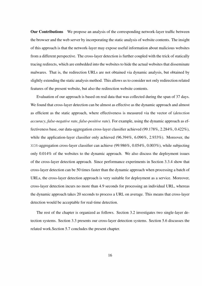
Our Contributions We propose an analysis of the corresponding network-layer traffic between

the browser and the web server by incorporating the static analysis of website contents. The insight

of this approach is that the network-layer may expose useful information about malicious websites

from a different perspective. The cross-layer detection is further coupled with the trick of statically

tracing redirects, which are embedded into the websites to hide the actual websites that disseminate

malwares. That is, the redirection URLs are not obtained via dynamic analysis, but obtained by

slightly extending the static analysis method. This allows us to consider not only redirection related

features of the present website, but also the redirection website contents.

Evaluation of our approach is based on real data that was collected during the span of 37 days.

We found that cross-layer detection can be almost as effective as the dynamic approach and almost

as efficient as the static approach, where effectiveness is measured via the vector of (detection

accuracy, false-negative rate, false-positive rate). For example, using the dynamic approach as ef-

fectiveness base, our data-aggregation cross-layer classifier achieved (99.178%, 2.284%, 0.422%),

while the application-layer classifier only achieved (96.394%, 6.096%, 2.933%). Moreover, the

XOR-aggregation cross-layer classifier can achieve (99.986%, 0.054%, 0.003%), while subjecting

only 0.014% of the websites to the dynamic approach. We also discuss the deployment issues

of the cross-layer detection approach. Since performance experiments in Section 3.3.4 show that

cross-layer detection can be 50 times faster than the dynamic approach when processing a batch of

URLs, the cross-layer detection approach is very suitable for deployment as a service. Moreover,

cross-layer detection incurs no more than 4.9 seconds for processing an individual URL, whereas

the dynamic approach takes 20 seconds to process a URL on average. This means that cross-layer

detection would be acceptable for real-time detection.

The rest of the chapter is organized as follows. Section 3.2 investigates two single-layer de-

tection systems. Section 3.3 presents our cross-layer detection systems. Section 5.6 discusses the

related work.Section 5.7 concludes the present chapter.

16

Data Analysis Methods In order to identify the better detection model, we consider four popular

machine learning algorithms: Naive Bayes, Logistic regression, Support Vector Machine (SVM)

and J48. Naive Bayes classifier is a probabilistic classifier based on Bayes’ rule [30]. Logistic

regression classifier [36] is a type of linear classifier, where the domain of the target variable is

0, 1. SVM classifier aims to find an maximum-margin hyperplane for separating different classes

in the training data [17]. We use the SMO (Sequential Minimal-Optimization) algorithm in our

experiment with polynomial kernel function [49]. J48 classifier is an implementation of C4.5

decision trees [52] for binary classification. These algorithms have been implemented in the Weka

toolbox [27], which also resolves issues such as missing feature data and conversion of strings to

numbers.

In order to know whether using a few features is as powerful as using all features and which

features are more indicative of malicious websites, we consider the following three feature selec-

tion methods. The first method is Principle Component Analysis (PCA), which transforms a set of

feature vectors to a set of shorter feature vectors [27]. The second feature selection method is called

“CfsSubsetEvalwith best-first search method" in the Weka toolbox [27], or Subset for short.

It essentially computes the features’ prediction power according to their contributions [26]. It out-

puts a subset of features, which are substantially correlated with the class but have low inter-feature

correlations. The third feature selection method is called “InfoGainAttributeEval with

ranker search method" in the Weka toolbox [27], or InfoGain for short. Its evaluation algorithm

essentially computes the information gain ratio (or more intuitively the importance of each fea-

ture) with respect to the class. Its selection algorithm ranks features based on their information

gains [19]. It outputs the ranks of all features in the order of decreasing importance.

3.2 Single-Layer Detection of Malicious Websites

In this section, we investigate two kinds of single-layer detection systems. One uses the application-

layer information only, and corresponds to the traditional static approach. The other uses the

network-layer information only, which is newly introduced in the present paper. The latter was

17

motivated by our insight that the network layer may expose useful information about malicious

websites from a different perspective. At each layer, we report the results obtained by using the

methodology described in Chapter 2.

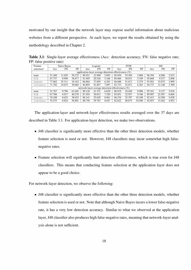
Table 3.1: Single-layer average effectiveness (Acc: detection accuracy; FN: false negative rate;FP: false positive rate)

Feature Naive Bayes Logistic SVM J48selection? Acc FN FP Acc FN FP Acc FN FP Acc FN FP

application-layer average detection effectiveness (%)none 51.260 11.029 59.275 90.551 22.990 5.692 85.659 55.504 3.068 96.394 6.096 2.933PCA 67.757 9.998 38.477 91.495 20.526 5.166 89.460 30.031 5.189 95.668 9.537 2.896Subset 77.962 35.311 18.162 86.864 37.895 6.283 84.688 51.671 5.279 93.581 15.075 3.999InfoGain 71.702 19.675 30.664 84.895 43.857 7.097 83.733 52.071 6.363 94.737 12.148 3.390

network-layer average detection effectiveness (%)none 51.767 0.796 61.645 90.126 21.531 6.630 86.919 24.449 9.986 95.161 9.127 3.676PCA 67.766 4.017 40.278 87.454 30.651 7.520 85.851 32.957 9.346 89.907 22.587 6.604Subset 70.188 0.625 38.035 88.141 25.629 8.061 86.534 25.397 10.188 92.415 14.580 5.658InfoGain 55.533 0.824 56.801 86.756 29.783 8.647 82.822 40.875 10.560 92.853 15.442 4.852

The application-layer and network-layer effectiveness results averaged over the 37 days are

described in Table 3.1. For application-layer detection, we make two observations.

• J48 classifier is significantly more effective than the other three detection models, whether

feature selection is used or not. However, J48 classifiers may incur somewhat high false-

negative rates.

• Feature selection will significantly hurt detection effectiveness, which is true even for J48

classifiers. This means that conducting feature selection at the application layer does not

appear to be a good choice.

For network-layer detection, we observe the following:

• J48 classifier is significantly more effective than the other three detection models, whether

feature selection is used or not. Note that although Naive Bayes incurs a lower false-negative

rate, it has a very low detection accuracy. Similar to what we observed at the application

layer, J48 classifier also produces high false-negative rates, meaning that network-layer anal-

ysis alone is not sufficient.

18

• Overall, feature selection hurts detection effectiveness. This also means that conducting

feature selection at the network layer is not a good approach.

By comparing the application layer and the network layer, we observed two interesting phe-

nomena. First, each single-layer detection method has some inherent limitation. Specifically, since

we were somewhat surprised by the high false-negative and false-positive rates of the single-layer

detection methods, we wanted to know whether they are caused by some outliers (extremely high

rates for some days), or are persistent over the 37 days. By looking into the data in detail, we

found that the false-negative and false-positive rates are reasonably persistent. This means that

single-layer detection has an inherent weakness.

Second, we observe that network-layer detection is only slightly less effective than application-

layer detection. This confirms our original insight that the network-layer traffic data can expose

useful information about malicious websites. Although network-layer detection alone is not suf-

ficient, this paved the way for exploring the utility of cross-layer detection of malicious websites,

which is explored in Section 3.3.

3.3 Cross-Layer Detection of Malicious Website

Having shown that network-layer traffic information can give approximately the same detection

effectiveness as the application layer, we now show how cross-layer detection can achieve much

better detection effectiveness. Given the pre-processed feature vectors at the application and net-

work layers, we extend the preceding methodology slightly to accommodate extra ideas that are

specific to cross-layer detection.

• Data-aggregation cross-layer detection: For a given URL, we obtain its cross-layer feature

vector by concatenating its application-layer feature vector and its network-layer feature vec-

tor. The resultant feature vectors are then treated as the pre-processed data in the methodol-

ogy described in Chapter 2 for further analysis.

• OR-aggregation cross-layer detection: For a given URL, if either the application-layer de-

19

tection model or the network-layer detection model says the URL is malicious, then the

cross-layer detection model says the URL is malicious; otherwise, the cross-layer detection

model says the URL is benign. This explains why we call this approach OR-aggregation.

• AND-aggregation cross-layer detection: For a given URL, if both the application-layer de-

tection model and the network-layer detection model say the URL is malicious, then the

cross-layer detection model says the URL is malicious; otherwise, the cross-layer detection

model says the URL is benign. This explains why we call this approach AND-aggregation.

• XOR-aggregation cross-layer detection: For a given URL, if both the application-layer de-

tection model and the network-layer detection model say the URL is malicious, then the

cross-layer detection model says the URL is malicious; if both the application-layer detec-

tion model and the network-layer detection model say the URL is benign, then the cross-layer

detection model says the URL is benign. Otherwise, the cross-layer detection model resorts

to the dynamic approach. That is, if the dynamic approach says the URL is malicious, then

the cross-layer detection model says the URL is malicious; otherwise, the cross-layer detec-

tion model says the URL is benign. We call this approach XOR-aggregation because it is in

the spirit of the XOR operation.

We stress that the XOR-aggregation cross-layer detection model resides in between the above three

cross-layer detection models and the dynamic approach because it partly relies on the dynamic ap-

proach. XOR-aggregation cross-layer detection is practical only when it rarely invokes the dynamic

approach.

3.3.1 Overall Effectiveness of Cross-Layer Detection

The effectiveness of cross-layer detection models, averaged over the 37 days, is described in Table

3.2, from which we make six observations discussed in the rest of this section.

First, data-aggregation cross-layer J48 classifier without using feature selection achieves (99.178%,

2.284%, 0.422%)-effectiveness, which is significantly better than the application-layer J48 classi-

20

fier that achieves (96.394%, 6.096%, 2.933%)-effectiveness, and is significantly better than the

network-layer J48 classifier that achieves (95.161%, 9.127%, 3.676%)-effectiveness. In other

words, cross-layer detection can achieve significantly higher effectiveness than the single-layer

detection models. This further confirms our motivational insight that the network-layer can expose

useful information about malicious websites from a different perspective. This phenomenon can

be explained by the low correlation between the application-layer feature vectors and the network-

layer feature vectors of the respective URLs. We plot the correlation coefficients in Figure 3.1,

which shows the absence of any correlation because the correlation coefficients fall into the inter-

val of (−0.4, 0.16]. This implies that the application layer and the network layer expose different

kinds of perspectives of malicious websites, and can be exploited to construct more effective de-

tection models.

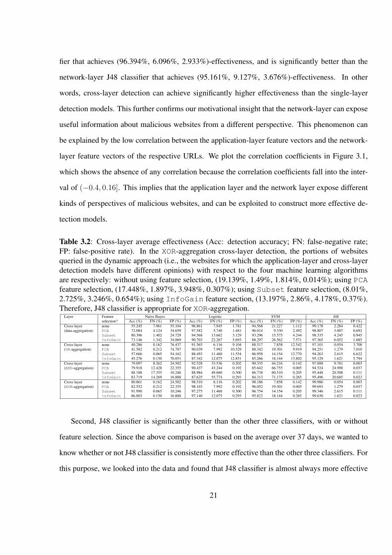
Table 3.2: Cross-layer average effectiveness (Acc: detection accuracy; FN: false-negative rate;FP: false-positive rate). In the XOR-aggregation cross-layer detection, the portions of websitesqueried in the dynamic approach (i.e., the websites for which the application-layer and cross-layerdetection models have different opinions) with respect to the four machine learning algorithmsare respectively: without using feature selection, (19.139%, 1.49%, 1.814%, 0.014%); using PCAfeature selection, (17.448%, 1.897%, 3.948%, 0.307%); using Subset feature selection, (8.01%,2.725%, 3.246%, 0.654%); using InfoGain feature section, (13.197%, 2.86%, 4.178%, 0.37%).Therefore, J48 classifier is appropriate for XOR-aggregation.

Layer Feature Naive Bayes Logistic SVM J48selection? Acc (%) FN (%) FP (%) Acc (%) FN (%) FP (%) Acc (%) FN (%) FP (%) Acc (%) FN (%) FP (%)

Cross-layer none 55.245 7.961 55.104 96.861 7.945 1.781 94.568 21.227 1.112 99.178 2.284 0.422(data-aggregation) PCA 72.084 4.124 34.659 97.582 5.740 1.481 96.014 9.330 2.492 98.807 3.007 0.692

Subset 80.396 1.402 24.729 94.568 13.662 3.129 93.296 15.575 4.244 98.335 4.245 0.945InfoGain 73.146 1.342 34.069 90.703 22.267 5.693 88.297 26.562 7.571 97.365 6.052 1.685

Cross-layer none 40.286 0.162 76.437 91.565 6.116 9.104 88.517 7.858 12.542 97.101 0.054 3.708(OR-aggregation) PCA 41.582 0.212 74.707 90.039 7.992 10.529 88.342 19.301 9.919 94.251 1.279 7.010

Subset 57.666 0.065 54.162 88.493 11.460 11.554 86.958 14.154 12.770 94.263 2.615 6.622InfoGain 45.276 0.150 70.051 87.342 12.075 12.851 85.266 18.144 13.802 95.129 1.621 5.794

Cross-layer none 79.097 8.262 24.502 92.528 33.536 0.202 90.335 44.216 0.142 97.888 9.781 0.003(AND-aggregation) PCA 79.918 12.428 22.355 90.437 43.244 0.192 85.642 66.755 0.005 94.524 24.998 0.037

Subset 88.188 17.355 10.246 88.984 49.660 0.300 86.738 60.510 0.205 95.448 20.508 0.111InfoGain 83.719 14.269 16.888 87.625 55.774 0.293 84.313 71.175 0.265 95.496 20.685 0.023

Cross-layer none 80.861 0.162 24.502 98.510 6.116 0.202 98.186 7.858 0.142 99.986 0.054 0.003(XOR-aggregation) PCA 82.552 0.212 22.355 98.103 7.992 0.192 96.052 19.301 0.005 99.693 1.279 0.037

Subset 91.990 0.065 10.246 97.275 11.460 0.300 96.754 14.154 0.205 99.346 2.615 0.111InfoGain 86.803 0.150 16.888 97.140 12.075 0.293 95.822 18.144 0.265 99.630 1.621 0.023

Second, J48 classifier is significantly better than the other three classifiers, with or without

feature selection. Since the above comparison is based on the average over 37 days, we wanted to

know whether or not J48 classifier is consistently more effective than the other three classifiers. For

this purpose, we looked into the data and found that J48 classifier is almost always more effective

21

-0.8

-0.4

0

0.4

0.8

5 10 15 20 25 30 35

co

rre

latio

n c

oe

ffic

ien

tday

MaxMin

Figure 3.1: The max and min correlation coefficients between application-layer and network-layerfeature vectors.

than the other three classifiers. Therefore, we recommend to use J48 classifier and will focus on

J48 classifier in the rest of the chapter.

Third, looking into the day-by-day effectiveness of cross-layer detection models with respect to

the InfoGain feature selection algorithm, we found the effect of feature selection to be persistent

over the 37 days, especially for the XOR-aggregation cross-layer detection model. This further

confirms that feature selection can be adopted in practice.

Fourth, the OR-aggregation cross-layer J48 classifier can achieve significantly lower false-

negative rate than the data-aggregation cross-layer J48 classifier, at the price of a lower detection

accuracy and a higher false-positive rate. On the other hand, the AND-aggregation cross-layer J48

classifier can achieve a significantly lower false-negative rate than the data-aggregation cross-layer

J48 classifier, at the price of a lower detection accuracy and a higher false-negative rate. This

phenomenon can be explained by using the definitions of the effectiveness metrics as follows. For

a fixed population of d1 malicious URLs and d2 benign URLs, a lower false-negative rate d1−d′1d1

implies a higher d′1. Since the detection accuracy d′1+d′2d1+d2

slightly decreases when compared with

the data-aggregation cross-layer detection, d′2 must decrease. This means that the false-positive

rate d2−d′2d2

increases. In a similar fashion, we can deduce that an increase in false-positive rate

can lead to a decrease in the false-negative rate. Thus, cross-layer classifiers offer a spectrum of

deployment possibilities, depending on security needs (e.g., a preference for lower false-negative

rate or lower false-positive rate). In Section 3.3.5, we will explore the deployment issues of the

22

cross-layer detection models.

Fifth, feature selection still hurts cross-layer detection effectiveness, but to a much lesser degree

than without feature selection. Indeed, the data-aggregation cross-layer J48 classifier with feature

selection is significantly better than the single-layer J48 classifier without using feature selection.

Moreover, the data-aggregation cross-layer J48 classifier with feature selection offers very high de-

tection accuracy and very low false-positive rate, the OR-aggregation cross-layer J48 classifier with

feature selection offers reasonably high detection accuracy and reasonably low false-negative rate,

and the AND-aggregation cross-layer J48 classifier with feature selection offers reasonably high

detection accuracy and extremely low false-positive rate. When compared with data-aggregation

cross-layer detection, OR-aggregation cross-layer detection has a lower false-negative rate, but a

lower detection accuracy and a higher false-positive rate. This can be explained as before.

Sixth and lastly, XOR-aggregation cross-layer detection can achieve almost the same effective-

ness as the dynamic approach. For example, it achieves (99.986%, 0.054%, 0.003%) effectiveness

without using feature selection, while only losing 100-99.086=0.014% accuracy to the dynamic ap-

proach. This means that the J48 classifier with XOR-aggregation can be appropriate for real-world

deployment. Also, note that the false-negative rate of the XOR-aggregation J48 classifier equals the

false-negative rate of the OR-aggregation J48 classifier. This is because all of the malicious web-

sites which are mistakenly classified as benign by the OR-aggregation J48 classifier are necessarily

mistakenly classified as benign by the XOR-aggregation J48 classifier. For a similar reason, we see

why the false-positive rate of the XOR-aggregation J48 classifier equals the false-positive rate of

the AND-aggregation J48 classifier.

3.3.2 Which Features Are Indicative?

Identifying the features that are most indicative of malicious websites is important because it can

deepen our understanding of malicious websites. Principal Components Analysis (PCA) has been

widely applied to obtain unsupervised feature selections by using linear dimensionality reduction

techniques. However, the PCA-based feature selection method is not appropriate to discover indi-

23

cations of malicious websites. Therefore, this research has focused on Subset and InfoGain.

The Subset feature selection algorithm This algorithm selects a subset of features with low

correlation while achieving high detection accuracy. Over the 37 days, this algorithm selected 15

to 16 (median: 16) features for the data-aggregation cross-layer detection, and 15 to 21 (median:

18) features for both the OR-aggregation and the AND-aggregation. Since this algorithm selects at

least 15 features daily, space limitation does not allow us to discuss the features in detail. Never-

theless, we will identify the few features that are also most commonly selected by the InfoGain

algorithm.

The InfoGain feature selection algorithm This algorithm ranks the contributions of indi-

vidual features. For each of the three specific cross-layer J48 classifiers and for each of the

37 days, we used this algorithm to select the 5 most contributive application-layer features and

the 4 most contributive network-layer features, which together led to the detection effectiveness

described in Table 3.2. The five most contributive application-layer features are (in descend-

ing order): (A1): URL_Length; (A5): Server; (A8): RegDate; (A6): Cache_control;

(A11): Stateprov. The four most contributive network-layer features are (in descending order):

(N11): Duration; (N9): Source_app_byte; (N13): Avg_remote_pkt_rate; (N2):

Dist_remote_TCP_port.

Intuitively, these features are indicative of malicious websites because during the compromise

of browsers, extra communications may be incurred for connecting to the redirection websites

while involving more remote TCP ports. We observed that most of the HTTP connections with

large (N11): Duration time are caused by slow HTTP responses. This is seemingly because

malicious websites usually employ dynamic DNS and Fast-Flush service network techniques to

better hide from detection. This would also explain why malicious websites often lead to larger

values of (N2): Dist_remote_TCP_port. We also observed that malicious websites often

have longer DNS query time (1.33 seconds on average) than benign websites (0.28 seconds on

average). This can be because the DNS information of benign websites is often cached in local

24

DNS servers, meaning there is no need to launch recursive or iterative DNS queries. Moreover, we

observe that malicious websites often incur smaller (N13): Avg_remote_pkt_rate because

the average volume of malicious website contents is often smaller than the average volume of

benign website contents. Our datasets show that the average volume of malicious website contents

is about 36.6% of the average volume of benign website contents.

The most commonly selected features Now we discuss the features that are most commonly

selected by both feature selection algorithms. On each of the 37 days, the Subset feature

selection algorithm selected the aforesaid 15-21 features of the 124 features. Overall, many

more features are selected by this algorithm over the 37 days. However, only 5 features were

selected every day, where 4 features are from the application layer and 1 feature is from the

network layer. Specifically, these features are: (A1): URL_Length; (A5): Server; (A2):

Number_of_special_characters_in_URL; (A13): Number_of_redirects; (N1):

Duration. These features are indicative of malicious websites because visiting malicious URLs

may cause the crawler to send multiple DNS queries and to connect to multiple web servers, which

could lead to a high volume of communications.

The InfoGain feature selection algorithm selected the aforesaid 15-16 features out of the

124 application-layer and network-layer features. Overall, only 17 of the 124 features were ever

selected, where 6 features are from the application layer and the other 11 features are from the

network layer. Three of the aforesaid features were selected every day: (A1): URL_Length, (N1):

Duration, (N9): Source_app_byte. As mentioned in the description of the InfoGain

feature selection algorithm, (N1): Duration represents one important feature of a malicious

web page. As for the (N9): Source_app_byte feature, intuitively, malicious web pages that

contain rich content (usually phishing contents) can cause multiple HTTP requests.

Overall, the features most commonly selected by the two feature selection algorithms are the

aforementioned (A1): URL_Length, (A5): Server and (N1): Duration. This further con-

firms the power of cross-layer detection. These features are indicative of malicious websites as

25

explained before.

3.3.3 How Did the Network Layer Help Out?

Previously, we observed the overall effectiveness of cross-layer detection, which at a high level can

be attributed to the fact that the network-layer data has a low correlation with the application-layer

data (i.e., the network-layer data does expose extra information about websites). Now we give a

deeper characterization of the specific contributions of the network-layer information that leads to

the correct classification of URLs.

Table 3.3: Breakdown of the average mis-classifications that were corrected by the network-layerclassifiers, where N/A means that the network-layer cannot help (see text for explanation).

Cross-layer aggregation method Average correction of FN Average correction of FPData-aggregation 79.59 13.91OR-aggregation 126.16 N/AAND-aggregation N/A 16.23XOR-aggregation 126.16 16.32

Table 3.3 summarizes the average number of “corrections" made through the network-layer

classifiers, where the average is taken over the 37 days. The mis-classifications by the application-

layer classifiers are either false-negative (i.e., the application-layer classifiers missed some mali-

cious URLs) or false-positive (i.e., the application-layer classifiers wrongly accused some benign

URLs). Note that for OR-aggregation, the network-layer classifiers cannot help correct the FP mis-

takes made by the application-layer classifiers because the benign URLs are always classified as

malicious as long as one classifier (in this case, the application-layer one) says they are malicious.

Similarly, for AND-aggregation, the network-layer classifiers cannot help correct the FN mistakes

made by the application-layer classifiers because (i) the malicious URLs are always classified

as benign unless both kinds of classifiers think they are malicious and (ii) the application-layer

classifier already says they are benign. We observe that the contributions of the network-layer

classifiers for XOR-aggregation in terms of correcting both FP and FN (126.16 and 16.32, respec-

tively) are strictly more significant than the contributions of the network-layer information for

26

data-aggregation (79.59 and 13.91, correspondingly). This explains why XOR-aggregation is

more effective than data-aggregation.

2

>1

A2

A18

A19

94

>26

>0

A17

A13

>2

1

A1

A1

A1

A16

76

>1

A2

>5

A8

=0

2010

benign

maliciousR R

R R

(a) Two mis-classification examples byapplication-layer classifier

2.48

>114

N11

N14

0.0062

N2N2

114

>1

N16

N15

164

N9

>1

N11

>1.35

N3

3

N12

>119.1

N9

<=8

>167

malicious

benign

(b) Network-layer corrections of the twoapplication-layer mis-classifications

Figure 3.2: Portions of the application-layer and network-layer classifiers corresponding to thetwo URLs.

In what follows we examine two example URLs that were mis-classified by the application-

layer classifier but corrected through the network-layer classifier. The two examples are among the

URLs on the first day data, where one example corresponds to the FP mistake (i.e., the application-

layer classifier mis-classified a benign URL as malicious) and the other example corresponds to the

FN mistake (i.e., the application-layer classifier mis-classified a malicious URL as benign). The

portion of the application-layer classifier corresponding to the two example URLs are highlighted

in Figure 3.2a, which involves the following features (in the order of their appearances on the

paths):

27

(A2) Number_of_special_char

(A18) Number_of_small_size_iframe

(A1) URL_length

(A19) Number_of_suspicious_JavaScript_functions

(A17) Number_iframe

(A13) number_of_redirect

(A16) Number_of_long_strings

(A8) register_date

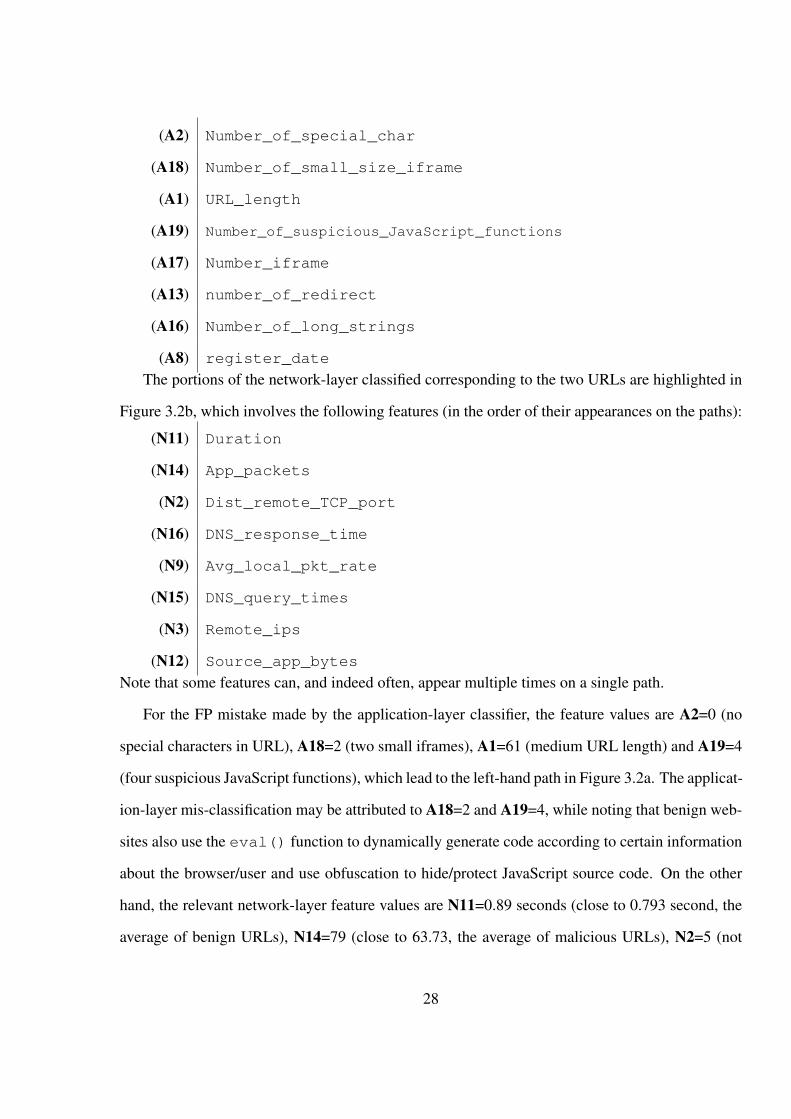
The portions of the network-layer classified corresponding to the two URLs are highlighted in

Figure 3.2b, which involves the following features (in the order of their appearances on the paths):

(N11) Duration

(N14) App_packets

(N2) Dist_remote_TCP_port

(N16) DNS_response_time

(N9) Avg_local_pkt_rate

(N15) DNS_query_times

(N3) Remote_ips

(N12) Source_app_bytes

Note that some features can, and indeed often, appear multiple times on a single path.

For the FP mistake made by the application-layer classifier, the feature values are A2=0 (no

special characters in URL), A18=2 (two small iframes), A1=61 (medium URL length) and A19=4

(four suspicious JavaScript functions), which lead to the left-hand path in Figure 3.2a. The applicat-

ion-layer mis-classification may be attributed to A18=2 and A19=4, while noting that benign web-

sites also use the eval() function to dynamically generate code according to certain information

about the browser/user and use obfuscation to hide/protect JavaScript source code. On the other

hand, the relevant network-layer feature values are N11=0.89 seconds (close to 0.793 second, the

average of benign URLs), N14=79 (close to 63.73, the average of malicious URLs), N2=5 (not

28

indicative because it is almost equally close to the averages of both benign URLs and malicious

URLs), N16=13.11ms (close to 13.29, the average of malicious URLs), N9=113 (close to 146, the

average of benign URLs), N15=6 (close to 7.36, the average of benign URLs). We observe that the

three network-layer features, namely N11, N9 and N15, played a more important role in correctly

classifying the URL.

For the FN mistake made by the application-layer classifier, A2=7 (close to 3.36, the average of

malicious URLs), A17=0 (indicating benign URL because there are no iframes), A13=0 (indicating

benign URL because there are no redirects), A1=22 (close to 18.23, the average of malicious

URLs), A16=2 (close to 0.88, the average of malicious URLs), and A8=2007 (indicating benign

URL because the domain name has been registered for multiple years). The above suggests that

A17, A13 and A8 played a bigger role in causing the mis-classification. On the other hand, the

relevant network feature values are N11=2.13 (close to 2.05, the average of malicious URLs),

N14=342 (close to 63.73, the average of malicious URLs), N2=7 (not very indicative because the

respective averages of benign URLs and malicious URLs are about the same), N3=3 (close to 2.40,

the average of benign URLs), N12=289 bytes (relatively close to 63.73, the average of malicious

URLs), and N9=423 (relatively close to 269, the average of malicious URLs). The above suggests

that the network-layer classifier can correct the mistake made by the application-layer classifier

because of features N11, N14, N12 and N9.

3.3.4 Performance Evaluation

As discussed in the Introduction, we aim to make our system as fast and scalable as the static

approach while achieving as high an effectiveness as the dynamic approach. In the preceding, we

have demonstrated that cross-layer J48 classifiers (indeed, all of the cross-layer detection models

we investigated) are almost as effective as the dynamic approach. In what follows we report that

the cross-layer J48 classifiers are much faster than the dynamic approach and almost as efficient as

the static approach.

The time spent on running our system consists of three parts: the time spent for collecting

29

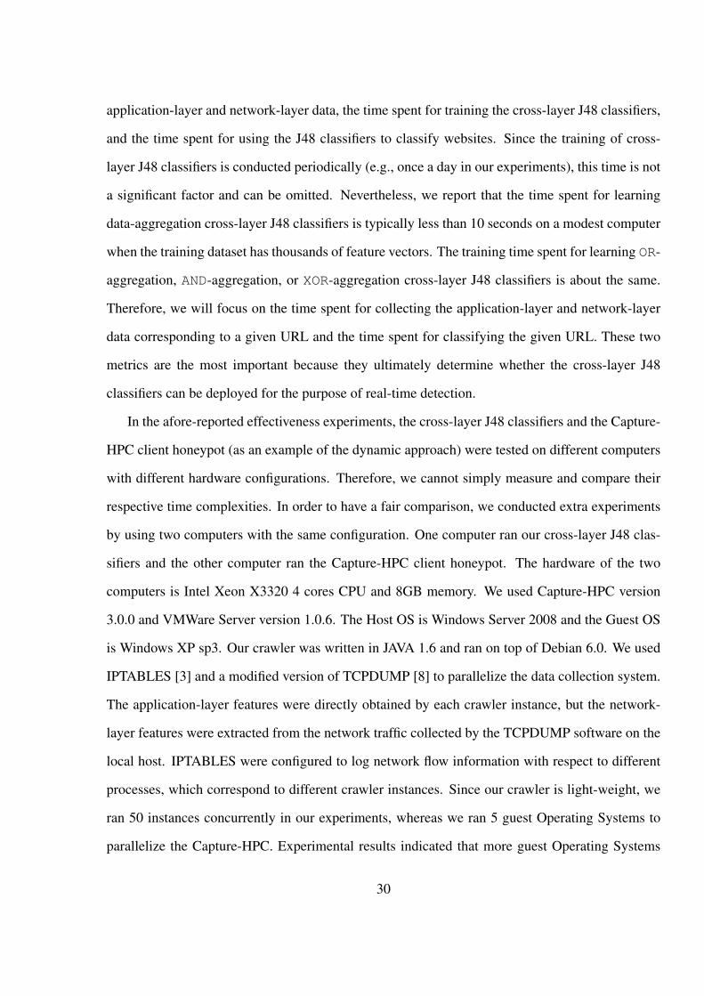
application-layer and network-layer data, the time spent for training the cross-layer J48 classifiers,

and the time spent for using the J48 classifiers to classify websites. Since the training of cross-

layer J48 classifiers is conducted periodically (e.g., once a day in our experiments), this time is not

a significant factor and can be omitted. Nevertheless, we report that the time spent for learning

data-aggregation cross-layer J48 classifiers is typically less than 10 seconds on a modest computer

when the training dataset has thousands of feature vectors. The training time spent for learning OR-

aggregation, AND-aggregation, or XOR-aggregation cross-layer J48 classifiers is about the same.

Therefore, we will focus on the time spent for collecting the application-layer and network-layer

data corresponding to a given URL and the time spent for classifying the given URL. These two

metrics are the most important because they ultimately determine whether the cross-layer J48

classifiers can be deployed for the purpose of real-time detection.

In the afore-reported effectiveness experiments, the cross-layer J48 classifiers and the Capture-

HPC client honeypot (as an example of the dynamic approach) were tested on different computers

with different hardware configurations. Therefore, we cannot simply measure and compare their

respective time complexities. In order to have a fair comparison, we conducted extra experiments

by using two computers with the same configuration. One computer ran our cross-layer J48 clas-

sifiers and the other computer ran the Capture-HPC client honeypot. The hardware of the two

computers is Intel Xeon X3320 4 cores CPU and 8GB memory. We used Capture-HPC version

3.0.0 and VMWare Server version 1.0.6. The Host OS is Windows Server 2008 and the Guest OS

is Windows XP sp3. Our crawler was written in JAVA 1.6 and ran on top of Debian 6.0. We used

IPTABLES [3] and a modified version of TCPDUMP [8] to parallelize the data collection system.

The application-layer features were directly obtained by each crawler instance, but the network-

layer features were extracted from the network traffic collected by the TCPDUMP software on the

local host. IPTABLES were configured to log network flow information with respect to different

processes, which correspond to different crawler instances. Since our crawler is light-weight, we

ran 50 instances concurrently in our experiments, whereas we ran 5 guest Operating Systems to

parallelize the Capture-HPC. Experimental results indicated that more guest Operating Systems

30

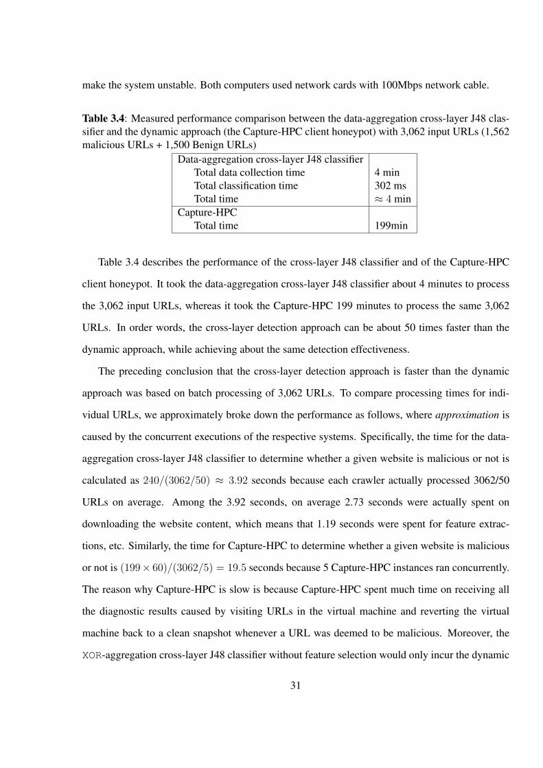
make the system unstable. Both computers used network cards with 100Mbps network cable.

Table 3.4: Measured performance comparison between the data-aggregation cross-layer J48 clas-sifier and the dynamic approach (the Capture-HPC client honeypot) with 3,062 input URLs (1,562malicious URLs + 1,500 Benign URLs)

Data-aggregation cross-layer J48 classifierTotal data collection time 4 minTotal classification time 302 msTotal time ≈ 4 min

Capture-HPCTotal time 199min

Table 3.4 describes the performance of the cross-layer J48 classifier and of the Capture-HPC

client honeypot. It took the data-aggregation cross-layer J48 classifier about 4 minutes to process

the 3,062 input URLs, whereas it took the Capture-HPC 199 minutes to process the same 3,062

URLs. In order words, the cross-layer detection approach can be about 50 times faster than the

dynamic approach, while achieving about the same detection effectiveness.

The preceding conclusion that the cross-layer detection approach is faster than the dynamic

approach was based on batch processing of 3,062 URLs. To compare processing times for indi-

vidual URLs, we approximately broke down the performance as follows, where approximation is

caused by the concurrent executions of the respective systems. Specifically, the time for the data-

aggregation cross-layer J48 classifier to determine whether a given website is malicious or not is

calculated as 240/(3062/50) ≈ 3.92 seconds because each crawler actually processed 3062/50

URLs on average. Among the 3.92 seconds, on average 2.73 seconds were actually spent on

downloading the website content, which means that 1.19 seconds were spent for feature extrac-

tions, etc. Similarly, the time for Capture-HPC to determine whether a given website is malicious

or not is (199× 60)/(3062/5) = 19.5 seconds because 5 Capture-HPC instances ran concurrently.

The reason why Capture-HPC is slow is because Capture-HPC spent much time on receiving all

the diagnostic results caused by visiting URLs in the virtual machine and reverting the virtual

machine back to a clean snapshot whenever a URL was deemed to be malicious. Moreover, the

XOR-aggregation cross-layer J48 classifier without feature selection would only incur the dynamic

31

approach to analyze, on average, about 5.04% × 3062 ≈ 154 websites. This means that even for

XOR-aggregation, the processing time per URL is no more than 3.92 + 19.5 × 154/3062 ≈ 4.9

seconds. Therefore, we conclude that even if the cross-layer detection system runs within each

individual computer, rather than a third-party server, it is about 4 times faster than the dynamic

approach. In any case, 4 seconds waiting time is arguably acceptable, especially since we can let

the browser start displaying the portions of website content that have no security concerns. This

is reasonable because the same idea has been used to give users the illusion that website contents

are displayed almost instantly, but actually it takes a few seconds to display the entire website

contents. On the other hand, waiting for 19.5 seconds for the dynamic approach to test whether a

website is malicious or not is not reasonable, which perhaps explains why the dynamic approach,

while powerful, is not used for real-time detection in practice.

3.3.5 Deployment

Cross-layer detection offers a spectrum of deployment options. It can be deployed as a stand-alone

solution because it is highly effective as analyzed before. Moreover, it can be deployed as a light-

weight front-end detection system of a bigger solution (see Figure 3.3), which aims at detecting as

many malicious websites as possible while scaling up to a large population of websites. For this

purpose, the data-aggregation and the OR-aggregation method would be efficient. Moreover, the

XOR-aggregation is particularly effective and should be deployed when it only incurs the back-end

dynamic approach occasionally.

There are several ways to deploy the physical components of the cross-layer detection ser-

vice. Recall that our system has three components: application-layer data collector (i.e., crawler),

network-layer traffic recorder, and cross-layer data correlator. The crawler takes URLs as input,

fetches the corresponding website contents, and conducts a light-weight analysis to identify the

redirects that are embedded into the website contents. The traffic recorder collects the network

traffic corresponding to the crawler’s activities in fetching the website contents. The cross-layer

data correlator relates the application-layer website contents to the corresponding network-layer

32

Our data collection system

Suspicious URLs

Client Honeypot-like

behavior-based detection &

possibly binary analysis

Input URL

Cross-layer detection of

malicious websites

Optional back-

end deeper

(slower)

analysis

Fast &

scalable

front-end

analysis

Data

collection

Cross-layer information

of webpages

Figure 3.3: Example deployment of the cross-layer detection system as the front-end of a big-ger solution because XOR-aggregation J48 classifiers achieve extremely high detection accuracy,extremely low false-negative and false-positive rates.

traffic via the input URLs. These components may or may not be deployed on the same physical

computer, as the following scenarios demonstrate.

First, we can deploy the stand-alone cross-layer detection system as a web browser plug-in. In

this case, the detection system can test whether the website is malicious or not before the browser

actually displays the website content. If it is malicious, the browser can take appropriate actions

according to a pre-determined policy (e.g., warning the user that the website is malicious). The

plug-in should collect the network-layer traffic corresponding to the application-layer website con-

tent of the given URL. The plug-in also may act as the network-layer traffic collector and the cross-

layer correlator. Moreover, network-traffic could be collected at some routers or gateways, from

which the plug-in can obtain the traffic corresponding to the application-layer website content.

Second, we can deploy the cross-layer detection system as an online service. This service

may be accessed by web browsers via the proxy or gateway technique. Specifically, when a user

browser points to a URL, the corresponding website will be analyzed by the cross-layer detection

service, which will then communicate the outcome back to the browser. The browser can take

33

appropriate actions based on its pre-determined policy (e.g., displaying the website or not).

Third, we can deploy the cross-layer detection system at the website hosting server itself. The

website hosting service vendor might have the incentive for proactively examining whether the

websites it hosts have been compromised, because this might enhance the reputation of the vendor.

In this case, the vendor can deploy it as a front-end to a bigger detection system, or deploy it as a

stand-alone system.

3.4 Related Work

Both industry and academia are actively seeking effective solutions to the problem of malicious

websites. Industry has mainly offered their proprietary blacklists of malicious websites, such as

Google’s Safe Browsing [1] and Mcafee’s SiteAdvisor [6]. Effectiveness of the blacklist approach

is fundamentally limited by the frequency at which the blacklists are updated and disseminated.

This justifies why we advocate pursuing light-weight real-time detection, which is the goal of the

present paper.

Researchers have used logistic regression to study phishing URLs [24], which does not consider

the issue of redirection. On the other hand, redirection has been used as an indicator of web

spams [10,45,51,64]. Kurt et al. [61] presented a system for scalably detecting spam contents. Ma

et al. [39, 40] studied how to detect phishing and spams based on URLs themselves.

In terms of detecting malicious websites that may host malwares, Choi et al. [16] investigated

the detection of malicious URLs, and Canali et al. [14] presented the design and implementation

of a static detection tool called Prophiler. However, these studies did not consider the usefulness of

cross-layer detection. On the other hand, the back-end system for deeper analysis is also an active

research topic [15, 18, 41, 67], because attackers have been attempting to circumvent dynamic

analysis [31, 53].

34

3.5 Summery

A key limitation of the present study is that, as pointed out in [31, 53] , the (back-end) dynamic

approach itself may have its own non-zero false-negative and false-positive rates. While studying

the dynamic approach is an orthogonal issue, we suggest a future study on the impact of false-

negatives and false-positives incurred in the dynamic approach, with an emphasis on Capture-HPC.

Another problem of interest for future work is to learn to what extent the effectiveness of cross-

layer detection systems can be improved by incorporating new techniques such as those described

in [18, 20, 46, 56].

Our cross-layer detection system provides a best-effort capability by statistically tracking the

redirects that are embedded into the website contents. It is difficult to statistically detect obfuscated

JavaScript-based redirects [22,23]. Even though the effectiveness of our cross-layer detection sys-

tem is almost as good as the dynamic approach, it would be useful in future work to determine the

impact of progress made in the direction of detecting obfuscated JavaScript-based redirects. This

is an important issue because, although our collected data hints that JavaScript-based redirection

is widely used by malicious websites, it appears that JavaScript obfuscation may not have been

widely used because our system can effectively detect the malicious URLs (almost as effectively

as the dynamic approach which is capable of dealing with redirects). However, this may not remain

true if in the future such redirects may be more widely exploited by the adversary. Fortunately, any

progress in dealing with obfuscated redirects can be adopted by our system in a plug-and-play

fashion.

To sum up, we presented a novel approach to detecting malicious websites based on the in-

sight that network-layer traffic data may expose useful information about websites, which may be

exploited to attain cross-layer detection of malicious websites. Experimental results showed that

cross-layer detection can achieve almost the same detection effectiveness, but about 50 times faster

than, the dynamic approach based on client honeypot systems. Moreover, the cross-layer detec-

tion systems can also be deployed to detect malicious websites in real time because the average

35

time for processing a website is approximately 4.9 seconds, which could be improved with some

engineering optimization.

36

Chapter 4: PROACTIVE DETECTION OF ADAPTIVE MALICIOUS

WEBSITES

4.1 Introduction

Compromising websites and abusing them to launch further attacks (e.g., drive-by-download [18,

50]) have become one of the mainstream attack methods. Unfortunately, it is infeasible, if not im-

possible, to prevent websites from being abused to launch attacks. This means that we must have

competent solutions that can detect compromised/malicious websites as soon as possible. This

is a difficult problem. Although client honeypots or their variants can detect malicious websites

with high accuracy, this dynamic approach often is too resource-consuming to be scalable. On the

other hand, the static approach aims to analyze the website contents without executing them in an

(emulated) browser. This approach is very efficient but has limited success in dealing with sophis-

ticated attacks. Recently, Xu et al. [65] (ACM CODASPY’13) proposed a promising cross-layer

method, which enhances the static approach by exploiting the corresponding network-layer traffic

that exposes some extra information about malicious websites. Using a dataset of 37 days, they

showed that their solution can almost achieve the best of both static detection (i.e., efficiency and

scalability) and dynamic detection (i.e., high accuracy, low false-positive, and low false-negative).

In this chapter, we investigate an inherent weakness of the static approach, namely that the

attacker can adaptively manipulate the contents of malicious websites to evade detection. The

manipulation operations can take place either during the process of, or after, compromising the

websites. This weakness is inherent because the attacker controls the malicious websites. Further-

more, the attacker can anticipate the machine learning algorithms the defender would use to train

its detection schemes (e.g., J48 classifiers or decision trees [52]), and therefore can use the same

algorithms to train its own version of the detection schemes. In other words, the defender has no

substantial “secret" that is not known to the attacker. This is in sharp contrast to the case of cryp-

tography, where the defender’s cryptographic keys are not known to the attacker. It is the secrecy

37

of cryptographic keys (as well as the mathematical properties of the cryptosystem in question) that

allows the defender to defeat various attacks.

The above discussion leads to the following question: how can we defeat adaptive attacks?

In this chapter, we make two contributions toward ultimately answering this question. First, we

formulate a model of adaptive attacks. The model accommodates attacker’s adaptation strate-

gies, manipulation constraints, and manipulation algorithms. Experiments based on a dataset of

40 days show that adaptive attacks can make malicious websites easily evade both single- and

cross-layer detections. Moreover, we find that the feature selection algorithms used by machine

learning algorithms do not select features of high security significance. In contrast, the adaptive

attack algorithms can select features of high security significance. Unfortunately, the “black-box"

nature of machine learning algorithms still makes it difficult to explain why some features are more

significant than others from a security perspective.

Second, we propose using proactive detection to counter adaptive attacks, where the defender

proactively trains its detection schemes. Experiments show that the proactive detection schemes

can detect manipulated malicious websites with significant success. Other findings include: (i) The

defender can always use proactive detection without worrying about the side-effects (e.g., when

the attacker is not adaptive). (ii) If the defender does not know the attacker’s adaptation strategy,

the defender should adopt what we call the full adaptation strategy, which appears (or is close) to

be a kind of equilibrium strategy as our preliminary analysis suggests.

The rest of the chapter is organized as follows. Section 4.2 investigates adaptive attacks and

their power. Section 4.3 explores proactive detection and its effectiveness against adaptive attacks.

Section 5.6 discusses related work. Section 5.7 concludes the chapter with future research direc-

tions.

Metrics. To evaluate the power of adaptive attacks and the effectiveness of proactive detection

against adaptive attacks, we mainly use the following metrics: detection accuracy, trust-positive

rate, false-negative rate, and false-positive rate. Let Dα = Dα.malicious ∪ Dα.benign be a set

of feature vectors that represent websites, where Dα.malicious represents the malicious websites

38

and Dα.benign represents the benign websites. Suppose a detection scheme (e.g., J48 classi-

fier) detects malicious ⊆ Dα.malicious as malicious websites and benign ⊆ Dα.benign as be-

nign websites. Detection accuracy is defined as |malicious∪benign||Dα| , true-positive rate is defined as

TP= |malicious||Dα.malicious| , false-negative rate is defined as TN= |Dα.malicious\malicious|

|Dα.malicious| , false-positive rate is

defined as FP= |Dα.benign\benign||Dα.benign| . Note that TP+FN=1, but we use both for better exposition of re-

sults.

Notations. The main notations are summarized as follows.

MLA machine learning algorithm

fv feature vector representing a website (and its redirects)

Xz feature Xz’s domain is [minz,maxz]

M0, . . . ,Mγ defender’s detection schemes (e.g., J48 classifier)

D′0 training data (feature vectors) for learning M0

D0 D0 = D0.malicious∪D0.benign, where malicious feature vectors in D0.malicious

may have been manipulated

D†0 feature vectors used by defender to proactively train M1, . . . ,Mγ ; D†

0 =

D†0.malicious ∪D†

0.benign

Mi(Dα) applying detection scheme Mi to feature vectors Dα

M0-γ(Dα) majority vote of M0(Dα),M1(Dα), . . . ,Mγ(Dα)

ST,C,F adaptation strategy ST, manipulation algorithm F, manipulation constraints C

sR← S assigning s as a random member of set S

v v is a node on a J48 classifier (decision tree), v.feature is the feature associated to

node v, and v.value is the “branching" point of v.feature’s value on the tree

4.2 Adaptive Attacks and Their Power

4.2.1 Adaptive Attack Model and Algorithm

The attacker can collect the same data as what is used by the defender to train a detection scheme.

The attacker knows the machine learning algorithm(s) the defender uses to learn a detection scheme

(e.g., J48 classifier or decision tree [52]), or even the defender’s detection scheme. To accommo-

39

date the worst-case scenario, we assume there is a single attacker that coordinates the compromise

of websites (possibly by many sub-attackers). This means that the attacker knows which websites

are malicious, while the defender aims to detect them. In order to evade detection, the attacker

can manipulate some features of the malicious websites. The manipulation operations can take

place during the process of compromising a website, or after compromising a website but before

the website is examined by the defender’s detection scheme.

More precisely, a website is represented by a feature vector. We call the feature vector repre-

senting a benign website benign feature vector, and malicious feature vector otherwise. Denote

by D′0 the defender’s training data, namely a set of feature vectors corresponding to a set of be-

nign websites (D′0.benign) and malicious websites (D′

0.malicious). The defender uses a machine

learning algorithm MLA to learn a detection scheme M0 from D′0 (i.e., M0 is learned from one

portion of D′0 and tested via the other portion of D′

0). As mentioned above, the attacker is given

M0 to accommodate the worst-case scenario. Denote by D0 the set of feature vectors that are to

be examined by M0 to determine which feature vectors (i.e., the corresponding websites) are ma-

licious. The attacker’s objective is to manipulate the malicious feature vectors in D0 into some Dα

so that M0(Dα) has a high false-negative rate, where α > 0 represents the number of rounds the

attacker conducts the manipulation operations.

The above discussion can be generalized to the adaptive attack model highlighted in Figure 4.1.

The model leads to adaptive attack Algorithm 1, which may call Algorithm 2 as a sub-routine.

Specifically, an adaptive attack is an algorithm AA(MLA,M0, D0, ST,C, F, α), where MLA and

M0 and D0 are described above, ST is the attacker’s adaptation strategy specified below, C is a set

of manipulation constraints (see Section 4.2.1), F is the attacker’s (deterministic or randomized)

manipulation algorithm (see Section 4.2.1), and α ≥ 1 is the number of rounds the attacker runs

F. Also as highlighted in Figure 4.1, we consider three basic adaptation strategies.

Parallel adaptation strategy: The attacker sets the manipulated Di = F(M0, D0,C), where i =

1, . . . , α, and F is a randomized manipulation algorithm, meaning that Di = Dj for i ̸= j is

unlikely.

40

!"#$%&' &'()

%& *&+,-./0/1

2

2

2

3

4"#$%&' &'()

5!"#$%&' &'()

6"#$%&' &'()

&7869,6:+-;;0<0,=

7.-0/0/16=->-

(a) Parallel adaptation strategy

!

" #$"%&'()*)+

,

,

,

-

.!

%&'()*)+

%&'()*)+

#!/ 0 "1#"!23

4#5/ 0 !1#!!23

# .!/ 0 .51# .5!23

# / 0 .!1# .!!23

#"6748&49%'::*;*&<

6('*)*)+4<'='

(b) Sequential adaptation strategy

!

" #$"%&'()*)+

,

,

,

-

.!

%&'()*)+

%&'()*)+

#!/ 0 "1#"123

#4/ 0 !1550#"1#!3123

# .!/ 0 .41550#"1-1# .43123

# 6/ 0 .!1550#"1-1# .!3123

#"7869&6:%';;*<*&=

7('*)*)+6='>'

(c) Full adaptation strategy

Figure 4.1: Adaptive attack algorithm AA(MLA,M0, D0, ST,C,F, α), where MLA is the de-fender’s machine learning algorithm, D′

0 is the defender’s training data, M0 is the defender’s de-tection scheme that is learned from D′

0 by using MLA, D0 is the feature vectors that are examinedby M0 in the absence of adaptive attacks, ST is the attacker’s adaptation strategy, C is a set ofmanipulation constraints, F is the attacker’s (deterministic or randomized) manipulation algorithmthat maintains the set of constraints C, α is the number of rounds the attacker runs its manipulationalgorithms. Dα is the manipulated version of D0 with malicious feature vectors D0.maliciousmanipulated. The attacker’s objective is make M0(Dα) have high false-negative rate.

Sequential adaptation strategy: The attacker sets the manipulated Di = F(Mi−1, Di−1,C) for

i = 1, . . . , α, where detection schemes M1, . . . ,Mα are respectively learned from D1, . . . , Dα

using the defender’s machine learning algorithm MLA (also known to the attacker).

Full adaptation strategy: The attacker sets the manipulated

Di = F(Mi−1,PP(D0, . . . , Di−1),C) for i = 1, 2, . . ., where PP(·, . . .) is a pre-processing algo-

rithm for “aggregating" sets of feature vectors D0, D1, . . . into a single set of feature vectors, F is

a manipulation algorithm, M1, . . . ,Mα are learned respectively from D1, . . . , Dα by the attacker

using the defender’s machine learning algorithm MLA. Algorithm 2 is a concrete implementation

of PP. Its idea is: since each malicious website corresponds to m malicious feature vectors that

respectively belong to D0, . . . , Dm−1, PP randomly picks one of the m malicious feature vectors

to represent the malicious website in D.

Note that it is possible to derive some hybrid attack strategies from the above three basic strate-

gies; we leave their study to future work. Note also that the attack strategies and manipulation

constraints are independent of the detection schemes, but manipulation algorithms would be spe-

41

Algorithm 1 Adaptive attack AA(MLA,M0, D0, ST,C,F, α)INPUT: MLA is defender’s machine learning algorithm, M0 is defender’s detection scheme, D0 =D0.malicious ∪ D0.benign where malicious feature vectors (D0.malicious) are to be manipulated (toevade detection of M0), ST is attacker’s adaptation strategy, C is a set of manipulation constraints, F isattacker’s manipulation algorithm, α is attacker’s number of adaptation roundsOUTPUT: Dα

1: initialize array D1, . . . , Dα

2: for i=1 to α do3: if ST == parallel-adaptation then4: Di ← F(M0, D0,C) {manipulated version of D0}5: else if ST == sequential-adaptation then6: Di ← F(Mi−1, Di−1,C) {manipulated version of D0}7: else if ST == full-adaptation then8: Di−1 ← PP(D0, . . . , Di−2) {see Algorithm 2}9: Di ← F(Mi−1,Di−1,C) {manipulated version of D0}

10: if i < α then11: Mi ← MLA(Di) {D1, . . . , Dα−1,M1, . . . ,Mα−1 are not used when

ST==parallel-adaptation}12: return Dα

Algorithm 2 Algorithm PP(D0, . . . , Dm−1)INPUT: m sets of feature vectors D0, . . . , Dm−1 where the zth malicious website corresponds toD0.malicious[z], . . . , Dm−1.malicious[z]OUTPUT: D = PP(D0, . . . , Dm−1)

1: D ← ∅2: size← sizeof(D0.malicious)3: for z = 1 to size do4: D[z] R← {D0.malicious[z], . . . , Dm−1.malicious[z]}5: D ← D ∪D0.benign6: return D

cific to the detection schemes.

Manipulation Constraints

There are three kinds of manipulation constraints. For a feature X whose value is to be manipu-

lated, the attacker needs to compute X.escape_interval, which is a subset of feature X’s domain

domain(X) and can possibly cause the malicious feature vector to evade detection. Specifically,

suppose features X1, . . . , Xj have been respectively manipulated to x1, . . . , xj (initially j = 0),

feature Xj+1’s manipulated value is randomly chosen from its escapte_interval, which is calcu-

lated using Algorithm 3, while taking as input Xj+1’s domain constraints, semantics constraints

42

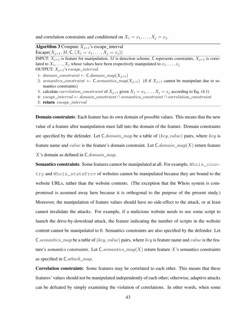
and correlation constraints and conditioned on X1 = x1, . . . , Xj = xj .

Algorithm 3 Compute Xj+1’s escape_intervalEscape(Xj+1,M,C, (X1 = x1, . . . , Xj = xj))

INPUT: Xj+1 is feature for manipulation, M is detection scheme, C represents constraints, Xj+1 is corre-lated to X1, . . . , Xj whose values have been respectively manipulated to x1, . . . , xjOUTPUT: Xj+1’s escape_interval

1: domain_constraint← C.domain_map(Xj+1)2: semantics_constraint ← C.semantics_map(Xj+1) {∅ if Xj+1 cannot be manipulate due to se-

mantics constraints}3: calculate correlation_constraint of Xj+1 given X1 = x1, . . . , Xj = xj according to Eq. (4.1)4: escape_interval← domain_constraint ∩ semantics_constraint ∩ correlation_constraint5: return escape_interval

Domain constraints: Each feature has its own domain of possible values. This means that the new

value of a feature after manipulation must fall into the domain of the feature. Domain constraints

are specified by the defender. Let C.domain_map be a table of (key, value) pairs, where key is

feature name and value is the feature’s domain constraint. Let C.domain_map(X) return feature

X’s domain as defined in C.domain_map.

Semantics constraints: Some features cannot be manipulated at all. For example, Whois_coun-

try and Whois_stateProv of websites cannot be manipulated because they are bound to the

website URLs, rather than the website contents. (The exception that the Whois system is com-

promised is assumed away here because it is orthogonal to the purpose of the present study.)

Moreover, the manipulation of feature values should have no side-effect to the attack, or at least

cannot invalidate the attacks. For example, if a malicious website needs to use some script to

launch the drive-by-download attack, the feature indicating the number of scripts in the website

content cannot be manipulated to 0. Semantics constraints are also specified by the defender. Let

C.semantics_map be a table of (key, value) pairs, where key is feature name and value is the fea-

ture’s semantics constraints. Let C.semantics_map(X) return feature X’s semantics constraints

as specified in C.attack_map.

Correlation constraints: Some features may be correlated to each other. This means that these

features’ values should not be manipulated independently of each other; otherwise, adaptive attacks

can be defeated by simply examining the violation of correlations. In other words, when some

43

features’ values are manipulated, the correlated features’ values should be accordingly manipulated

as well. That is, feature values are manipulated either for evading detection or for maintaining the

constraints. Correlation constraints can be automatically derived from data on demand (as done

in our experiments), or alternatively given as input. Let C.group be a table of (key, value) pairs,

where key is feature name and value records the feature’s correlated features. Let C.group(X)

return the set of features belonging to C.group, namely the features that are correlated to X .

Now we describe a method for maintaining correlation constraints, which is used in our ex-

periments. Suppose D0 = D0.malicious ∪ D0.benign is the input set of feature vectors, where

the attacker knows D0.malicious and attempts to manipulate the malicious feature vectors (repre-

senting malicious websites). Suppose the attacker already manipulated D0 into Di and is about to

manipulate Di into Di+1, where initial manipulation corresponds to i = 0. Suppose X1, . . . , Xm

are some features that are strongly correlated to each other, where “strong" means that the Pear-

son correlation coefficient is greater than a threshold (e.g., 0.7). To accommodate the worst-case

scenario, we assume that the threshold parameter is set by the defender and given to the attacker.

It is natural and simple to identify and manipulate features one-by-one. Suppose without loss of

generality that features X1, . . . , Xj (j < m) have been manipulated, where j = 0 corresponds

to the initial case, and that the attacker now needs to manipulate feature Xj+1’s value. For this

purpose, the attacker derives from data D′0 a regression function:

Xj+1 = β0 + β1X1 + . . .+ βjXj + ϵ

for some unknown noise ϵ. Given (X1, . . . , Xj) = (x1, . . . , xj), the attacker can compute

x̂j+1 = β0 + β1x1 + . . .+ βjxj.

Suppose the attacker wants to maintain the correlation constraints with a confidence level θ (e.g.,

θ = .85) that is known to the defender and the attacker (for accommodating the worst-case sce-

44

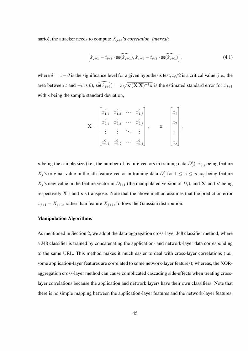
nario), the attacker needs to compute Xj+1’s correlation_interval:

[x̂j+1 − tδ/2 · ̂se(x̂j+1), x̂j+1 + tδ/2 · ̂se(x̂j+1)

], (4.1)

where δ = 1−θ is the significance level for a given hypothesis test, tδ/2 is a critical value (i.e., the

area between t and −t is θ), ̂se(x̂j+1) = s√x′(X′X)−1x is the estimated standard error for x̂j+1

with s being the sample standard deviation,

X =

x01,1 x0

1,2 · · · x01,j

x02,1 x0

2,2 · · · x02,j

...... . . . ...

x0n,1 x0

n,2 · · · x0n,j

, x =

x1

x2

...

xj

,

n being the sample size (i.e., the number of feature vectors in training data D′0), x

0z,j being feature

Xj’s original value in the zth feature vector in training data D′0 for 1 ≤ z ≤ n, xj being feature

Xj’s new value in the feature vector in Di+1 (the manipulated version of Di), and X′ and x′ being

respectively X’s and x’s transpose. Note that the above method assumes that the prediction error

x̂j+1 −Xj+1, rather than feature Xj+1, follows the Gaussian distribution.

Manipulation Algorithms

As mentioned in Section 2, we adopt the data-aggregation cross-layer J48 classifier method, where

a J48 classifier is trained by concatenating the application- and network-layer data corresponding

to the same URL. This method makes it much easier to deal with cross-layer correlations (i.e.,

some application-layer features are correlated to some network-layer features); whereas, the XOR-

aggregation cross-layer method can cause complicated cascading side-effects when treating cross-

layer correlations because the application and network layers have their own classifiers. Note that

there is no simple mapping between the application-layer features and the network-layer features;

45

otherwise, the network-layer data would not expose any useful information beyond what is already

exposed by the application-layer data [65]. Specifically, we present two manipulation algorithms,

called F1 and F2, which exploit the defender’s J48 classifier to guide the manipulation of features.

Both algorithms neither manipulate the benign feature vectors (which are not controlled by the

attacker), nor manipulate the malicious feature vectors that are already classified as benign by the

defender’s detection scheme (i.e., false-negative). Both algorithms may fail, while brute-forcing

may fail as well because of the manipulation constraints.

The notations used in the algorithms are: for node v in the classifier, v.feature is the feature

associated to node v, and v.value is v.feature’s “branching" value as specified by the classifier

(a binary tree with all features numericalized). For feature vector fv, fv.feature.value denotes the

value of feature feature in fv. The data structure

S = {(feature, value, interval,manipulated)},

keeps track of the features that are associated to the nodes in question, S.features is the set of

features recorded in S, S.feature.value is the feature’s value recorded in S, S.feature.interval

is the feature’s interval recorded in S, S.feature.manipulated == true means S.feature

has been manipulated. A feature vector fv is actually manipulated according to S only when the

manipulation can mislead M to misclassify the manipulated fv as benign.

Algorithm 4 describes manipulation algorithm F1(M,D,C), where M is a J48 classifier and

D is a set of feature vectors, and C is the manipulation constraints. The basic idea is the follow-

ing: For every malicious feature vector in D, there is a unique path (in the J48 classifier M ) that

leads to a malicious leaf, which indicates that the feature vector is malicious. We call the path

leading to malicious leaf a malicious path, and the path leading to a benign leaf (which indicates

a feature vector as benign) a benign path. By examining the path from the malicious leaf to the

root, say malicious_leaf → v2 → . . . → root, and identifying the first inner node, namely

v2, the algorithm attempts to manipulate fv.(v2.feature).value so that the classification can lead

46

Algorithm 4 Manipulation algorithm F1(M,D,C)INPUT: J48 classifier M (binary decision tree), feature vector set D = D.malicious ∪D.benign, manip-ulation constraints COUTPUT: manipulated feature vectors

1: for all feature vector fv ∈ D.malicious do2: mani← true; success← false; S ← ∅3: v be the root node of M4: while (mani == true) AND (success == false) do5: if v is an inner node then6: if fv.(v.feature).value ≤ v.value then7: interval← [minv.feature, v.value]8: else9: interval← (v.value,maxv.feature]

10: if ̸ ∃(v.feature, ·, ·, ·) ∈ S then11: S ← S ∪ {(v.feature,

fv.(v.feature).value, interval, false)}12: else13: S.(v.feature).interval← interval ∩

S.(v.feature).interval14: v ← v’s child as determined by v.value and fv.(v.feature).value15: else if v is a malicious leaf then16: v∗ ← v.parent17: S∗ ← {s ∈ S : s.manipulated == true}18: {X1, . . . , Xj} ← C.group(v∗.feature) ∩ S∗.features, with values x1, . . . , xj w.r.t. S∗

19: esc_interval← Escape(v∗.feature,M,C, (X1 = x1, . . . , Xj = xj)) {call Algorithm 3}20: if esc_interval == ∅ then21: mani← false

22: else23: denote v∗.feature by X {for shorter presentation}24: S.X.interval← (esc_interval ∩ S.X.interval)

25: S.X.valueR← S.X.interval

26: S.X.manipulated← true

27: v ← v’s sibling28: else29: success← true {reaching a benign leaf}30: if (mani == true) AND (success == true) AND (MR(M,C, S) == true) then31: update fv’s manipulated features according to S32: return set of manipulated feature vectors D

47

to malicious_leaf ’s sibling, say v2,another_child, which is guaranteed to exist (otherwise, v2 can-

not be an inner node). Note that there must be a sub-path rooted at v2,another_child that leads to a

benign_leaf (otherwise, v2 cannot be an inner node as well), and that manipulation of values of

the features corresponding to the nodes on the sub-tree rooted at v2,another_child will preserve the

postfix v2 → . . . → root. For each feature vector fv ∈ D.malicious, the algorithm may success-

fully manipulate some features’ values while calling Algorithm 5 to maintain constraints, or fail

because the manipulations cannot be conducted without violating the constraints. The worst-case

time complexity of F1 is O(hℓg), where h is the height of the J48 classifier, ℓ is the number of

features, and g is the size of the largest group of correlated features. The actual time complexity

is very small. In our experiments on a laptop with Intel X3320 CPU and 8GB RAM memory, F1

takes 1.67 milliseconds to process a malicious feature vector on average over all malicious feature

vectors and over 40 days.

Algorithm 5 Maintaining constraints MR(M,C, S)

INPUT: J48 classifier M , manipulation constraints C, S = {(feature, value, interval,manipulated)}OUTPUT: true or false

1: S∗ ← {s ∈ S : s.manipulated == true}2: for all (feature, value, interval, true) ∈ S do3: for all X ∈ C.group(feature) \ S∗.features do4: {X1, . . . , Xj} ← C.group(feature) ∩ S∗.features, whose values are respectively x1, . . . , xj

w.r.t. S∗

5: escape_interval← Escape(feature,M,C, (X1 = x1, . . . , Xj = xj))6: if escape_interval == ∅ then7: return false

8: else9: X.interval← escape_interval

10: X.valueR← X.interval

11: S∗ ← S∗ ∪ {(X,X.value,X.interval, true)}12: return true

Now let us look at one example. At a high-level, the attacker runs AA(“J48”,M0, D0, ST,C, F1,

α = 1) and therefore F1(M0, D0,C) to manipulate the feature vectors, where ST can be any of the

three strategies because they cause no difference when α = 1 (see Figure 4.1 for a better exposi-

tion). Consider the example J48 classifier M in Figure 4.2, where features and their values are for

illustration purpose, and the leaves are decision nodes with class 0 indicating benign leaves and 1

48

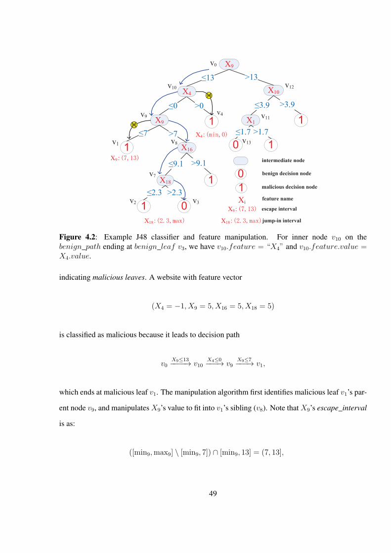
≤0

≤13

>0

X9

X4

X9

X16

X18

≤7 >7

≤9.1

≤2.3 >2.3

X10

X1

R R

R R

>13

≤3.9

X9

X4

v4

v2 v3

v7

v8v1

v9

v12v10

v11

v0

X18

≤1.7 >1.7

>3.9

>9.1

v13

intermediate node

benign decision node

Xifeature name

malicious decision node

escape intervalX9

X18 jump-in interval

Figure 4.2: Example J48 classifier and feature manipulation. For inner node v10 on thebenign_path ending at benign_leaf v3, we have v10.feature = “X4” and v10.feature.value =X4.value.

indicating malicious leaves. A website with feature vector

(X4 = −1, X9 = 5, X16 = 5, X18 = 5)

is classified as malicious because it leads to decision path

v0X9≤13−−−−→ v10

X4≤0−−−→ v9X9≤7−−−→ v1,

which ends at malicious leaf v1. The manipulation algorithm first identifies malicious leaf v1’s par-

ent node v9, and manipulates X9’s value to fit into v1’s sibling (v8). Note that X9’s escape_interval

is as:

([min9,max9] \ [min9, 7]) ∩ [min9, 13] = (7, 13],

49

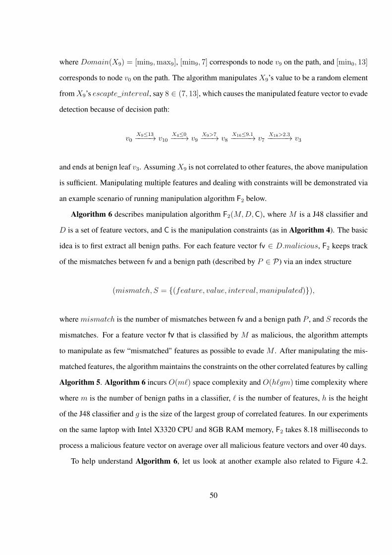
where Domain(X9) = [min9,max9], [min9, 7] corresponds to node v9 on the path, and [min0, 13]

corresponds to node v0 on the path. The algorithm manipulates X9’s value to be a random element

from X9’s escapte_interval, say 8 ∈ (7, 13], which causes the manipulated feature vector to evade

detection because of decision path:

v0X9≤13−−−−→ v10

X4≤0−−−→ v9X9>7−−−→ v8

X16≤9.1−−−−−→ v7X18>2.3−−−−−→ v3

and ends at benign leaf v3. Assuming X9 is not correlated to other features, the above manipulation

is sufficient. Manipulating multiple features and dealing with constraints will be demonstrated via

an example scenario of running manipulation algorithm F2 below.

Algorithm 6 describes manipulation algorithm F2(M,D,C), where M is a J48 classifier and

D is a set of feature vectors, and C is the manipulation constraints (as in Algorithm 4). The basic

idea is to first extract all benign paths. For each feature vector fv ∈ D.malicious, F2 keeps track

of the mismatches between fv and a benign path (described by P ∈ P) via an index structure

(mismatch, S = {(feature, value, interval,manipulated)}),

where mismatch is the number of mismatches between fv and a benign path P , and S records the

mismatches. For a feature vector fv that is classified by M as malicious, the algorithm attempts

to manipulate as few “mismatched" features as possible to evade M . After manipulating the mis-

matched features, the algorithm maintains the constraints on the other correlated features by calling

Algorithm 5. Algorithm 6 incurs O(mℓ) space complexity and O(hℓgm) time complexity where

where m is the number of benign paths in a classifier, ℓ is the number of features, h is the height

of the J48 classifier and g is the size of the largest group of correlated features. In our experiments

on the same laptop with Intel X3320 CPU and 8GB RAM memory, F2 takes 8.18 milliseconds to

process a malicious feature vector on average over all malicious feature vectors and over 40 days.

To help understand Algorithm 6, let us look at another example also related to Figure 4.2.

50

Consider feature vector

(X4 = .3, X9 = 5.3, X16 = 7.9, X18 = 2.1, X10 = 3, X1 = 2.3),

which is classified as malicious because of path

v0X9≤13−−−−→ v10

X4>0−−−→ v4.

To evade detection, the attacker can compare the feature vector to the matrix of two benign pathes.

For the benign path v3 → v7 → v8 → v9 → v10 → v0, the feature vector has three mismatches,

namely features X4, X9, X18. For the benign path v13 → v11 → v12 → v0, the feature vector has

two mismatches, namely X9 and X1. The algorithm first processes the benign path ending at node

v13. For the benign path ending at node v13, the algorithm manipulates X9 to a random value in

[13,max9] (say 17), and manipulates X1 to a random value in X1.interval = [min1, 1.7] (say 1.4).

Suppose X9, X10, X1 are strongly correlated to each other. the algorithm further calculates X10’s

escape interval according to Eq. (4.1) while considering the constraint X10 ∈ [min10, 3.9] (see

node v12). Suppose X10 is manipulated to 3.5 after accommodating the correlation constraints. In

this scenario, the manipulated feature vector is

(X4 = .3, X9 = 17, X16 = 7.9, X18 = 2.1, X10 = 3.5, X1 = 1.4),

which is classified as benign because of path

v0X9>13−−−−→ v12

X10≤3.9−−−−−→ v11X1≤1.7−−−−→ v13.

Suppose on the other hand, that X10 cannot be manipulated to a value in [min10, 3.9] without

violating the constraints. The algorithm stops with this benign path and considers the benign path

end at node v3. If the algorithm fails with this benign path again, the algorithm will not manipulate

51

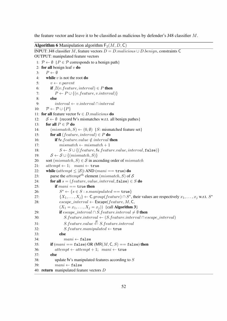
the feature vector and leave it to be classified as malicious by defender’s J48 classifier M .

Algorithm 6 Manipulation algorithm F2(M,D,C)INPUT: J48 classifier M , feature vectors D = D.malicious ∪D.benign, constraints COUTPUT: manipulated feature vectors

1: P ← ∅ {P ∈ P corresponds to a benign path}2: for all benign leaf v do3: P ← ∅4: while v is not the root do5: v ← v.parent6: if ̸ ∃(v.feature, interval) ∈ P then7: P ← P ∪ {(v.feature, v.interval)}8: else9: interval← v.interval ∩ interval

10: P ← P ∪ {P}11: for all feature vector fv ∈ D.malicious do12: S ← ∅ {record fv’s mismatches w.r.t. all benign pathes}13: for all P ∈ P do14: (mismatch, S)← (0, ∅) {S: mismatched feature set}15: for all (feature, interval) ∈ P do16: if fv.feature.value /∈ interval then17: mismatch← mismatch+ 118: S ← S ∪ {(feature, fv.feature.value, interval, false)}19: S ← S ∪ {(mismatch, S)}20: sort (mismatch, S) ∈ S in ascending order of mismatch21: attempt← 1; mani← true

22: while (attempt ≤ |S|) AND (mani == true) do23: parse the attemptth element (mismatch, S) of S24: for all s = (feature, value, interval, false) ∈ S do25: if mani == true then26: S∗ ← {s ∈ S : s.manipulated == true}27: {X1, . . . , Xj} ← C.group(feature) ∩ S∗, their values are respectively x1, . . . , xj w.r.t. S∗

28: escape_interval← Escape(feature,M,C,(X1 = x1, . . . , Xj = xj)) {call Algorithm 3}

29: if escape_interval ∩ S.feature.interval ̸= ∅ then30: S.feature.interval← (S.feature.interval ∩ escape_interval)

31: S.feature.valueR← S.feature.interval

32: S.feature.manipulated← true

33: else34: mani← false

35: if (mani == false) OR (MR(M,C, S) == false) then36: attempt← attempt+ 1; mani← true

37: else38: update fv’s manipulated features according to S39: mani← false

40: return manipulated feature vectors D

52

4.2.2 Power of Adaptive Attacks

In order to evaluate the power of adaptive attacks, we evalute M0(D1), where M0 is learned from

D′0 and D1 is the output of adaptive attack algorithm AA. Our experiments are based on a 40-

day dataset, where for each day: D′0 consists of 340–722 malicious websites (with mean 571)

as well as 2,231–2,243 benign websites (with mean 2,237); D0 consists of 246–310 malicious

websites (with mean 282) as well as 1,124–1,131 benign websites (with mean 1,127). We focus

on the data-aggregation cross-layer method, while considering single-layer (i.e., application and

network) method for comparison purpose. We first highlight some manipulation constraints that

are enforced in our experiments.

Domain constraints: The length of URLs (URL_Length) cannot be arbitrarily manipulated be-

cause it must include hostname, protocol name, domain name and directories. Similarly, the length

of webpage content (Content_length) cannot be arbitrarily short.

Correlation constraints: There are four groups of application-layer features that are strongly cor-

related to each other; there are three groups of network-layer features that are strongly correlated to

each other; there are three groups of features that formulate cross-layer constraints. One group of

cross-layer correlation is: the application-layer website content length (Number_of_Content

_length) and the network-layer duration time (Duration). This is because the bigger the

content, the longer the fetching time. Another group of cross-layer correlations is: the application-

layer number of redirects (Number_of_redirect), the network-layer number of DNS queries

(Number

_of_DNS_query), the network-layer number of DNS answers (Number_of_DNS_answer).

This is because more redirects leads to more DNS queries and more DNS answers.

Semantics constraints: Assuming the Whois system is not compromised, the following features

cannot be manipulated: website registration date (RegDate), website registration state/province

(Stateprov), website registration postal code (Postalcode), and website registration country

(Country). For malicious websites that use some scripts to launch the drive-by-download attack,

53

the number of scripts contained in the webpage contents (Number_of_Scripts) cannot be 0.

The application-layer protocol feature (Protocol) may not be arbitrarily changed (e.g., from ftp

to http).

Table 4.1: Experiment results with M0(D1) in terms of average false-negative rate (FN), averagenumber of manipulated features (Number_of_MF), average percentage of failed attempts (FA),where “average" is over the 40 days of the dataset mentioned above.

F1 F2

FN Number_of_MF FA FN Number_of_MF FAnetwork-layer 94.7% 4.31 5.8% 95.3% 4.01 5.1%application-layer 91.9% 6.01 8.6% 93.3% 5.23 7.1%data-agg. cross-layer 87.6% 7.23 12.6% 89.1% 6.19 11.0%

Table 4.1 summarizes the results of adaptive attack AA(“J48”,M0, D0, ST,C, F, α = 1) based

on the 40-day dataset mentioned above, where C accommodates the constraints mentioned above.

The experiment can be more succinctly represented as M0(D1), meaning that the defender is static

(or non-proactive) and the attacker is adaptive with α = 1, where D1 is the manipulated version of

D0. Note that in the case of α = 1, the three adaptation strategies lead to the same D1 as shown

in Figure 4.1. From Table 4.1, we make the following observations. First, both manipulation

algorithms can effectively evade detection by manipulating on average 4.31-7.23 features while

achieving false-negative rate 87.6%-94.7% for F1, and by manipulating on average 4.01-6.19 fea-

tures while achieving false-negative rate 89.1%-95.3% for F2. For the three J48 classifiers based

on different kinds of D0 (i.e., network-layer data alone, application-layer data alone and cross-

layer data-aggregation), F2 almost always slightly outperforms F1 in terms of false-negative rate

(FN), average number of manipulated features (Number_of_MF), and average percentage of failed

attempts at manipulating feature vectors (FA). Second, data-aggregation cross-layer classifiers are

more resilient against adaptive attacks than network-layer classifiers as well as application-layer

classifiers.

Now we ask: Which features are often manipulated for evasion? We notice that many

features are manipulated over the 40 days, but only a few are manipulated often. For application-

layer alone, F1 most often (i.e., > 150 times each day for over the 40 days) manipulates the

following five application-layer features: URL length (URL_Length), number of scripts con-

54

tained in website content (Number_of_Script), webpage length (Content_length), num-

ber of URLs embedded into the website contents (Number_of_Embedded_URL), and number

of Iframes contained in the webpage content (Number_of_Iframe). In contrast, F2 most often

(i.e., > 150 times) manipulates the following three application-layer features: number of special

characters contained in URL (Number_of_Special_character), number of long strings

(Number_of_Long_strings) and webpage content length (Content_length). That is,

Content_length is the only feature that is most often manipulated by both algorithms.

For network-layer alone, F1 most often (i.e., > 150 times) manipulates the following three fea-

tures: number of remote IP addresses (Number_of_Dist_remote_IP), duration time (Dura-

tion), and number of application packets (Number_of_Local_app_packet). Whereas, F2

most often (i.e., > 150 times) manipulates the distinct number of TCP ports used by the remote

servers (Number_of_Dist_remote_TCP_port). In other words, no single feature is often

manipulated by both algorithm.

For data-aggregation cross-layer detection, F1 most often (i.e., > 150 times each day for

over the 40 days) manipulates three application-layer features — URL length (URL_Length),

webpage length (Content_length), number of URLs embedded into the website contents

(Number_of_Embedded_URLs) — and two network-layer features — duration time (Durat-

ion) and number of application packets (Number_of_Local_app_packet). On the other

hand, F2 most often (i.e., > 150 times) manipulates two application-layer features — number

of special characters contained in URL (Number_of_Special_characters) and webpage

content length (Content length) — and one network-layer feature — duration time (Durat-

ion). Therefore, Content_length and Duration are most often manipulated by both algo-

rithms.

The above discrepancy between the frequencies that features are manipulated can be attributed

to the design of the manipulation algorithms. Specifically, F1 seeks to manipulate features that

are associated to nodes that are close to the leaves. In contrast, F2 emphasizes on the mismatches

between a malicious feature vector and an entire benign path, which represents a kind of global

55

search and also explains why F2 manipulates fewer features.

Table 4.2: Experiment results of M0(D1) by treating as non-manipulatable the InfoGain-selectedfive application-layer features and four network-layer features. Metrics are as in Table 4.1.

F1 F2

FN Number_of_MF FA FN Number_of_MF FAnetwork-layer 93.1% 4.29 7.5% 95.3% 4.07 5.1%application-layer 91.3% 6.00 9.2% 93.3% 5.28 7.1%data-aggregation 87.4% 7.22 12.7% 89.1% 6.23 11.0%

Having identified the features that are often manipulated, the next natural question is: Why

them? Or: Are they some kind of “important" features? It would be ideal if we can directly

answer this question by looking into the most-often manipulated features. Unfortunately, this is a

difficult problem because J48 classifiers (or most, if not all, detection schemes based on machine

learning), are learned in a black-box (rather than white-box) fashion. As an alternative, we compare

the manipulated features to the features that would be selected by a feature selection algorithm for

the purpose of training classifiers. To be specific, we use the InfoGain feature selection algorithm

because it ranks the contributions of individual features [65]. We find that among the manipu-

lated features, URL_Length is the only feature among the five InfoGain-selected application-

layer features, and Number_of_Dist_remote_TCP_port is the only feature among the four

InfoGain-selected network-layer features. This suggests that the feature selection algorithm does

not necessarily offer good insights into the importance of features from a security perspective.

To confirm this, we further conduct the following experiment by additionally treating InfoGain-

selected tops features as semantics constraints in C (i.e., they cannot be manipulated). Table 4.2

(counterparting Table 4.1) summarizes the new experiment results. By comparing the two tables,

we observe that there is no significant difference between them, especially for manipulation algo-

rithm F2. This means that InfoGain-selected features have little security significance.

Table 4.3: Experiment results of M0(D1) by treating the features that were manipulated by adap-tive attack AA as non-manipulatable. Notations are as in Tables 4.1-4.2.

F1 F2

FN Number_of_MF FA FN Number_of_MF FAnetwork-layer 62.1% 5.88 41.6% 80.3% 5.07 21.6%application-layer 68.3% 8.03 33.7% 81.1% 6.08 20.1%data-aggregation 59.4% 11.13 41.0% 78.7% 7.83 21.5%

56

In order to know whether or not the adaptive attack algorithm AA actually manipulated some

“important" features, we conduct an experiments by setting the most-often manipulated features

as non-manipulatable. The features that are originally identified by F1 and then set as non-

manipulatable are: webpage length (content_length), number of URLs that are embedded

into the website contents (Number_of_Embedded_URLs), number of redirects (Number_of

_redirect), number of distinct TCP ports that are used by the remote webservers (Dist_rem-

ote_tcp_port), and number of application-layer packets (Local_app_packets). Table 4.3

summarizes the results. When compared with Tables 4.1-4.2, we see that the false-negative rate

caused by adaptive attacks drops substantially: from about 90% down to about 60% for manipu-

lation algorithm F1, and from about 90% down to about 80% for manipulation algorithm F2. This

means perhaps that the features that are originally identified by F1 are more indicative of malicious

websites than the features that are originally identified by F2. Moreover, we note that no feature

is manipulated more than 150 times and only two features — Number_of_Iframe (the num-

ber of iframes) and Number_of_DNS_query (the number of DNS query) — are manipulated

more than 120 times by F1 and one feature — Number_of_suspicous_JS_function (the

number of JavaScript functions) — is manipulated more than 120 times by F2.

4.3 Proactive Defense against Adaptive Attacks

We have showed that adaptive attacks can ruin the defender’s (non-proactive) detection schemes.

Now we investigate how the defender can exploit proactive defense against adaptive attacks. We

propose that the defender can run the same kinds of manipulation algorithms to proactively antici-

pate the attacker’s adaptive attacks.

4.3.1 Proactive Defense Model and Algorithm

Proactive defense PD(MLA,M0, D†0, Dα, STD,C,FD, γ) is described as Algorithm 7, which calls

as a sub-routine the proactive training algorithm PT described in Algorithm 8 (which is similar

to, but different from, the adaptive attack algorithm AA). Specifically, PT aims to derive detection

57

Algorithm 7 Proactive defense PD(MLA,M0, D†0, Dα, STD,C, FD, γ)

INPUT: M0 is learned from D′0 using machine learning algorithm MLA, D†

0 = D†0.benign∪D

†0.malicious,

Dα (α unknown to defender) is set of feature vectors (with Dα.malicious possibly manipulated by theattacker), STD is defender’s adaptation strategy, FD is defender’s manipulation algorithm, C is set of con-straints, γ is defender’s number of adaptations roundsOUTPUT: malicious vectors fv ∈ Dα

1: M †1 , . . . ,M

†γ ← PT(MLA,M0, D

†0, STD,C,FD, γ) {see Algorithm 8}

2: malicious← ∅3: for all fv ∈ Dα do4: if (M0(fv) says fv is malicious) OR (majority of M0(fv),M

†1(fv), . . . ,M

†γ(fv) say fv is malicious)

then5: malicious← malicious ∪ {fv}6: return malicious

schemes M †1 , . . . ,M

†γ from the starting-point detection scheme M0. Since the defender does not

know a priori whether the attacker is adaptive or not (i.e., α > 0 vs. α = 0), PD deals with this

uncertainty by first applying M0, which can deal with D0 effectively. If M0 says that a feature

vector fv ∈ Dα is malicious, fv is deemed malicious; otherwise, a majority voting is made between

M0(fv),M†1(fv), . . . ,M

†γ(fv).

Algorithm 8 Proactive training PT(MLA,M0, D†0, STD,C,FD, γ)

INPUT: same as in Algorithm 7OUTPUT: M †

1 , . . . ,M†γ

1: M †0 ←M0 {for simplifying notations}

2: initialize D†1, . . . , D

†γ and M †

1 , . . . ,M†γ

3: for i=1 to γ do4: if STD == parallel-adaptation then5: D†

i .malicious← FD(M†0 , D

†0.malicious,C)

6: else if STD == sequential-adaptation then7: D†

i .malicious← FD(M†i−1, D

†i−1.malicious,C)

8: else if STD == full-adaptation then9: D†

i−1.malicious← PP(D†0, . . . , D

†i−2)

10: D†i .malicious← FD(M

†i−1,D

†i−1,C)

11: D†i .benign← D†

0.benign

12: M †i ← MLA(D†

i )

13: return M †1 , . . . ,M

†γ

58

4.3.2 Evaluation and Results

To evaluate proactive defense PD’s effectiveness, we use Algorithm 9 and the metrics defined in

Chapter 2: detection accuracy (ACC), trust-positive (TP), false-negative (FN), and false-positive

(FP). Note that TP=1-FN, but we still list both for easing the discussion. When the other parameters

are clear from the context, we use M0-γ(Dα) to stand for Eva(MLA,M0, D†0, D0, STA, FA, STD,FD,

C, α, γ). For each of the 40 days mentioned above, the data for proactive training, namely D†0, con-

sists of 333–719 malicious websites (with mean 575) and 2,236–2,241 benign websites (with mean

2,238).

The parameter space of Eva includes at least 108 scenarios: the basic adaptation strategy space

STA × STD is 3× 3 (i.e., not counting any hybrids of parallel-adaptation, sequential-

adaptation and full-adapatation), the manipulation algorithm space FA × FB is 2 × 2, and

the adaptation round parameter space is at least 3 (α >,=, < γ). Since the data-aggregation cross-

layer detection significantly outperforms the single layer detections against non-adaptive attacks

[65] and is more resilient than the single layer detections against adaptive attacks as shown in

Section 4.2.2, in what follows we focus on data-aggregation cross-layer detection. For the baseline

case of non-proactive detection against non-adaptive attack, namely M0(D0), we have average

ACC = 99.68% (detection accuracy), TP =99.21% (true-positive rate), FN=0.79% (false-negative

rate) and FP=0.14% (false-positive rate), where “average" is over the 40 days corresponding to the

dataset. This baseline result also confirms the conclusion in [65], namely that data-aggregation

cross-layer detection can be used in practice, and justifies why we use it in this chapter.

Table 4.4 summarizes the effectiveness of proactive defense against adaptive attacks. We make

the following observations. First, if the defender is proactive (i.e., γ > 0) but the attacker is non-

adaptive (i.e., α = 0), the false-negative rate drops from 0.79% in the baseline case to some number

belonging to interval [0.23%, 0.56%]. The price is: the detection accuracy drops from 99.68% in

the baseline case to some number belonging to interval [99.23%, 99.68%] the false-positive rate

increases from 0.14% in the baseline case to some number belonging to interval [0.20%, 0.93%],

59

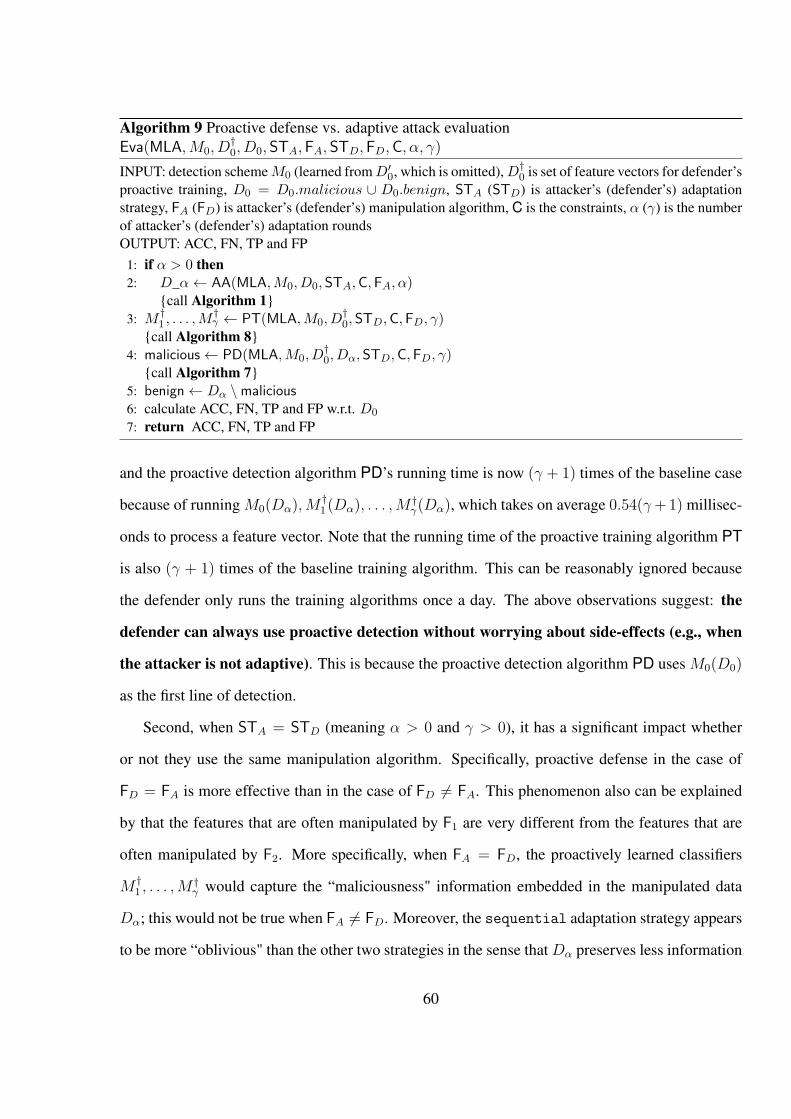
Algorithm 9 Proactive defense vs. adaptive attack evaluationEva(MLA,M0, D

†0, D0, STA, FA, STD,FD,C, α, γ)

INPUT: detection scheme M0 (learned from D′0, which is omitted), D†

0 is set of feature vectors for defender’sproactive training, D0 = D0.malicious ∪ D0.benign, STA (STD) is attacker’s (defender’s) adaptationstrategy, FA (FD) is attacker’s (defender’s) manipulation algorithm, C is the constraints, α (γ) is the numberof attacker’s (defender’s) adaptation roundsOUTPUT: ACC, FN, TP and FP

1: if α > 0 then2: D_α← AA(MLA,M0, D0, STA,C,FA, α)

{call Algorithm 1}3: M †

1 , . . . ,M†γ ← PT(MLA,M0, D

†0, STD,C,FD, γ)

{call Algorithm 8}4: malicious← PD(MLA,M0, D

†0, Dα,STD,C,FD, γ)

{call Algorithm 7}5: benign← Dα \malicious6: calculate ACC, FN, TP and FP w.r.t. D0

7: return ACC, FN, TP and FP

and the proactive detection algorithm PD’s running time is now (γ + 1) times of the baseline case

because of running M0(Dα),M†1(Dα), . . . ,M

†γ(Dα), which takes on average 0.54(γ+1) millisec-

onds to process a feature vector. Note that the running time of the proactive training algorithm PT

is also (γ + 1) times of the baseline training algorithm. This can be reasonably ignored because

the defender only runs the training algorithms once a day. The above observations suggest: the

defender can always use proactive detection without worrying about side-effects (e.g., when

the attacker is not adaptive). This is because the proactive detection algorithm PD uses M0(D0)

as the first line of detection.

Second, when STA = STD (meaning α > 0 and γ > 0), it has a significant impact whether

or not they use the same manipulation algorithm. Specifically, proactive defense in the case of

FD = FA is more effective than in the case of FD ̸= FA. This phenomenon also can be explained

by that the features that are often manipulated by F1 are very different from the features that are

often manipulated by F2. More specifically, when FA = FD, the proactively learned classifiers

M †1 , . . . ,M

†γ would capture the “maliciousness" information embedded in the manipulated data

Dα; this would not be true when FA ̸= FD. Moreover, the sequential adaptation strategy appears

to be more “oblivious" than the other two strategies in the sense that Dα preserves less information

60

Table 4.4: Data-aggregation cross-layer proactive detection with STA = STD. For baseline caseM0(D0), ACC = 99.68%, true-positive rate TP =99.21%, false-negative rate FN=0.79%, and false-positive rate FP=0.14%.

Strat. Manipulation algorithm M0-8(D0) M0-8(D1) M0-8(D9)ACC TP FN FP ACC TP FN FP ACC TP FN FP

FD = F1 vs. FA = F1 99.59 99.71 0.29 0.39 95.58 92.03 7.97 3.62 95.39 92.00 8.00 3.83FD = F1 vs. FA = F2 99.27 99.77 0.23 0.77 78.51 25.50 74.50 9.88 78.11 32.18 67.82 11.48

PARFD = F2 vs. FA = F1 99.16 99.76 0.24 0.93 76.33 19.32 80.68 11.17 78.96 39.77 60.23 12.14FD = F2 vs. FA = F2 99.59 99.62 0.38 0.39 93.66 90.25 9.75 5.59 96.17 92.77 7.23 3.08FD = F1 vs. FA = F1 99.52 99.69 0.31 0.45 93.44 77.48 22.52 3.05 92.04 59.33 30.67 2.99FD = F1 vs. FA = F2 99.23 99.70 0.30 0.82 74.24 20.88 79.22 14.06 79.43 30.03 69.97 9.38

SEQFD = F2 vs. FA = F1 99.27 99.67 0.33 0.80 77.14 29.03 70.97 12.33 82.72 40.93 59.07 7.83FD = F2 vs. FA = F2 99.52 99.53 0.47 0.50 93.44 78.70 21.30 2.10 92.04 62.30 37.70 2.11FD = F1 vs. FA = F1 99.68 99.44 0.56 0.20 96.92 96.32 3.68 2.89 95.73 92.03 7.97 3.27FD = F1 vs. FA = F2 99.27 99.58 0.42 0.72 85.68 40.32 59.68 4.38 78.11 29.99 70.01 11.00

FULLFD = F2 vs. FA = F1 99.60 99.66 0.34 0.40 85.65 51.84 48.16 6.93 87.61 72.99 27.01 9.01FD = F2 vs. FA = F2 99.68 99.60 0.40 0.28 96.92 95.60 4.40 2.88 95.73 90.09 9.91 2.83

about D0. This may explain why the false-negative rates when STA = STD = sequential can

be respectively substantially higher than their counterparts when STA = STD ̸= sequential.

The above discussions suggest the following: If the attacker is using STA = sequential, the

defender should not use STD = sequential.

Table 4.5: Data-aggregation cross-layer proactive detection against adaptive attacks with FD =FA.

STD vs. STA M0-γ(Dα)STA = parallel STA = sequential STA = full

ACC TP FN FP ACC TP FN FP ACC TP FN FP

Manipulation algorithm FD = FA = F1

STD = PARM0-8(D1) 95.58 92.03 7.97 3.62 94.25 90.89 9.11 4.96 94.91 92.08 7.92 4.32M0-8(D9) 95.39 92.00 8.00 3.83 92.38 80.03 19.97 4.89 93.19 84.32 15.68 4.54

STD = SEQM0-8(D1) 92.15 74.22 25.78 3.93 93.44 77.48 22.52 3.05 92.79 76.32 23.68 3.07M0-8(D9) 89.20 58.39 41.61 4.11 92.04 59.33 30.67 2.99 88.42 57.89 42.11 3.91

STD = FULLM0-8(D1) 96.24 94.98 5.02 3.42 96.46 94.99 5.01 3.15 96.92 96.32 3.68 2.89M0-8(D9) 94.73 90.01 9.99 4.21 94.70 90.03 9.97 4.23 95.73 92.03 7.97 3.27

Manipulation algorithm FD = FA = F2

STD = PARM0-8(D1) 93.66 90.25 9.75 5.59 94.25 88.91 11.09 3.98 94.91 89.77 10.23 3.53M0-8(D9) 96.17 92.77 7.23 3.08 92.38 77.89 22.11 4.32 93.19 81.32 18.68 3.38

STD = SEQM0-8(D1) 90.86 70.98 29.02 4.82 93.44 78.70 21.30 2.10 92.79 72.32 27.68 4.02M0-8(D9) 88.43 53.32 46.68 3.97 92.04 62.30 37.70 2.11 88.42 57.88 42.12 3.17

STD = FULLM0-8(D1) 95.69 93.89 6.11 3.88 96.46 94.98 5.02 3.03 96.92 95.60 4.40 2.88M0-8(D9) 96.06 91.46 8.54 2.89 94.70 90.99 9.01 2.32 95.73 90.09 9.91 2.83

Third, what adaptation strategy should the defender use to counter STA = sequential? Table

4.5 shows that the defender should use STD = full because it leads to relatively high detection

accuracy and relatively low false-negative rate, while the false-positive rate is comparable to the

other cases. Even if the attacker knows that the defender is using STD = full, Table 4.5 shows

that the attacker does not have an obviously more effective counter adaptation strategy. This hints

61

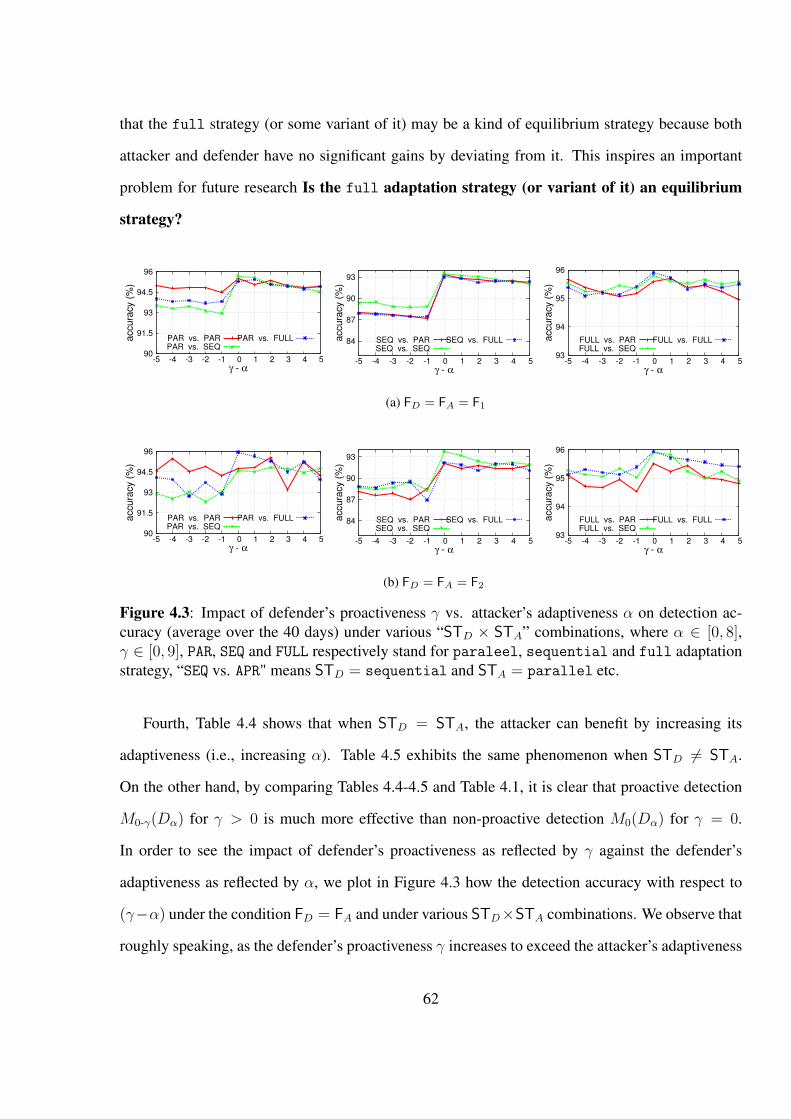
that the full strategy (or some variant of it) may be a kind of equilibrium strategy because both

attacker and defender have no significant gains by deviating from it. This inspires an important

problem for future research Is the full adaptation strategy (or variant of it) an equilibrium

strategy?

90

91.5

93

94.5

96

-5 -4 -3 -2 -1 0 1 2 3 4 5

accura

cy (

%)

γ - α

PAR vs. PARPAR vs. SEQ

PAR vs. FULL 84

87

90

93

-5 -4 -3 -2 -1 0 1 2 3 4 5

accura

cy (

%)

γ - α

SEQ vs. PARSEQ vs. SEQ

SEQ vs. FULL

93

94

95

96

-5 -4 -3 -2 -1 0 1 2 3 4 5

accura

cy (

%)

γ - α

FULL vs. PARFULL vs. SEQ

FULL vs. FULL

(a) FD = FA = F1

90

91.5

93

94.5

96

-5 -4 -3 -2 -1 0 1 2 3 4 5

accura

cy (

%)

γ - α

PAR vs. PARPAR vs. SEQ

PAR vs. FULL 84

87

90

93

-5 -4 -3 -2 -1 0 1 2 3 4 5

accura

cy (

%)

γ - α

SEQ vs. PARSEQ vs. SEQ

SEQ vs. FULL

93

94

95

96

-5 -4 -3 -2 -1 0 1 2 3 4 5accura

cy (

%)

γ - α

FULL vs. PARFULL vs. SEQ

FULL vs. FULL

(b) FD = FA = F2

Figure 4.3: Impact of defender’s proactiveness γ vs. attacker’s adaptiveness α on detection ac-curacy (average over the 40 days) under various “STD × STA” combinations, where α ∈ [0, 8],γ ∈ [0, 9], PAR, SEQ and FULL respectively stand for paraleel, sequential and full adaptationstrategy, “SEQ vs. APR" means STD = sequential and STA = parallel etc.

Fourth, Table 4.4 shows that when STD = STA, the attacker can benefit by increasing its

adaptiveness (i.e., increasing α). Table 4.5 exhibits the same phenomenon when STD ̸= STA.

On the other hand, by comparing Tables 4.4-4.5 and Table 4.1, it is clear that proactive detection

M0-γ(Dα) for γ > 0 is much more effective than non-proactive detection M0(Dα) for γ = 0.

In order to see the impact of defender’s proactiveness as reflected by γ against the defender’s

adaptiveness as reflected by α, we plot in Figure 4.3 how the detection accuracy with respect to

(γ−α) under the condition FD = FA and under various STD×STA combinations. We observe that

roughly speaking, as the defender’s proactiveness γ increases to exceed the attacker’s adaptiveness

62

α (i.e., γ changes from γ < α to γ = α to γ > α), the detection accuracy may have a significant

increase at γ − α = 0. Moreover, we observe that when STD = full, γ − α has no significant

impact on the detection accuracy. This suggest that the defender should always use the full

adaptation strategy to alleviate the uncertainty about the attacker’s adaptiveness α.

4.4 Related Work

The most closely related work is the cross-layer framework for detecting malicious websites pro-

posed by Xu et al. [65]. Their study appears to be motivated by the following observation: Static

analysis technique (e.g., by analyzing URLs and/or webpage contents) for detecting malicious

websites can achieve the highest performance and scalability, but not effective; whereas dynamic

analysis technique (i.e., by analyzing the runtime behavior of website contents in monitored envi-

ronment) can achieve the highest effectiveness, but not performance or scalability. They proposed

exploiting the network “lens" (i.e., looking into the network-layer traffic that corresponding to their

static data collection) to obtain extra information about the websites, where the extra information

may be useful to enhance the effectiveness of static detection technique. The effectiveness met-

rics they consider are: detection accuracy, false-positive rate and false-negative rate. The showed

indeed that by additionally taking advantage of the network “lens" they can almost achieve the

best of both static detection technique (i.e., performance and scalability) and dynamic detection

technique (i.e., effectiveness).

Another factor that may have contributed to the success and performance of their cross-layer

detection is that they statically parse website contents to catch redirects. While static parsing

can only achieve best-effort guarantee only because of the difficulty in dealing with obfuscated

JavaScript-based redirects [23], which is nevertheless an orthogonal research problem and can

benefit from any future studies in this category [66]. Finally, Invernizzi et al. [29] proposed a

novel method for quickly identifying malicious websites, which can be used to replace the method

of identifying malicious websites for training purpose — downloading blacklisted websites and

analyzing their maliciousness using the dynamic approach — in a modular fashion.

63

Taking a broader view, the problem of detecting malicious websites have been investigated by

both industry and academia. For example, industrial solutions include McAfee’s Site Advisor [2]

and Google’s Safe Browsing [1]. Prior academic investigations on the detection of malicious

websites include Prophiler [14] and others (e.g., [16]). Dynamic detection techniques such as

Client Hopeypot have been investigated in [15, 18, 41, 67]. There are ongoing research activities

on making dynamic analysis techniques resistant against sophisticated attacks [33, 53]. Loosely

related to our study are the investigations on detecting Phishing websites [24, 39, 40], detecting

spams [10, 39, 40, 45, 51, 61, 64], detecting suspicious URLs embedded in twitter message streams

[57], and dealing with browser-related attacks [37, 59]. All these studies did not consider the idea

of cross-layer detection introduced in [65].

Our study of proactive defense vs. adaptive attack is closely related to the problem of adversar-

ial machine learning, where the attacker aims to evade an detection mechanism that is derived from

some machine learning method [9,62]. In the context of unsupervised learning for anomaly detec-

tion, Perdisci et al. [48] investigated how to make the detection harder to evade. In the context of

supervised learning, existing studies fall into two categories. In the first category, the attacker can

poison/manipulate the training data. Existing studies for tackling this problem include [44,47,55].

In the second category, the training data is not poisoned. There are two scenarios. First, the

attacker has black-box access to the detection mechanism and attempts to evade detection after

making, ideally, as few as possible queries to the detection mechanism. This setting has been stud-

ied in [38, 43]. Second, the attacker has access to the detection mechanism, which is true for our

resilience study. Dalvi et al. [21] used Game Theoretic method to study this problem in the setting

of spam detection. Our model actually gives the attacker more freedom because the attacker knows

the data the defender collected.

4.5 Summary

We formulated a model of adaptive attacks by which the attacker can manipulate the malicious

websites under its control to evade detection. We also formulated a model of proactive defense

64

against the adaptive attacks. Experimental results based on a 40-day dataset shows that adaptive

attacks can easily evade non-proactive defense, but can be effectively countered by proactive de-

fense.

This study introduces a set of interesting research problems: Is the full adaptation strategy

indeed a kind of equilibrium strategy? What is the optimal manipulation algorithm (if exists)?

How can we precisely characterize the evadability caused by adaptive attacks in this context?

65

Chapter 5: CHARACTERIZING AND DETECTING EVOLVING

MALICIOUS WEBSITES

5.1 Introduction

Compromising websites and subsequently abusing them to launch further attacks (e.g., drive-by-

download [18,50]) has become one of the mainstream attack vectors. Unfortunately, it is infeasible,

if not impossible, to completely eliminate such attacks, meaning that we must have competent solu-

tions that can detect compromised/malicious websites as soon as possible. It is therefore important

to understand how the threats may evolve. In this chapter we present a statistical characterization

of the evolution of malicious websites. Such characterization studies can lead to a deeper under-

standing about the threat landscape. More specifically, we focus on two aspects: What are the

statistical evolution characteristics of malicious websites? For how long a newly learned detectin

model will remain effective?

5.2 Our Contributions

We make the following contributions. First, we characterize the detection accuracy of Mi(Dj),

where Mi is the detection model trained using the data collected on day i, Dj is the (testing) data

collected on day j. We find that despite that Mi(Di) is highly effective in terms of accuracy,

false-positive rate, and false-negative rate, Mi(Dj) for i ̸= j is not.

Second, we propose using online learning to cope with the evolution of malicious websites. Our

experiments show that online learning can effectively deal with evolving malicious websites. We

also develop an online learning algorithm with a real-time adaptation strategy, which automatically

refreshes the training dataset when some criteria are met.

The rest of the chapter is organized as follows. Section 5.3 briefly describes the dataset we

analyze. Section 5.4 investigates the evolution of malicious websites and the security implications.

Section 5.5 characterize the distribution of Di. Section 5.6 discusses related prior work. Section

66

5.7 concludes the chapter with future research directions.

5.3 Data Description

The input candidate URLs consist of two categories: malicious websites and benign websites. As

defined in Chapter 2, a malicious website is a website that launches drive-by-download attacks

(perhaps coupled with website redirects). The terms malicious URLs and malicious websites are

used interchangeably. In this chapter, websites features are the application-layer and network-layer

ones defined in Chapter 2.

The dataset consists of benign and malicious websites for a period of 160 consecutive days,

between 09/19/2013 and 02/25/2013. On each day, our training data consists of 498–877 malicious

websites (with mean 599) and 6798–6810 benign websites (with mean 6800); our cross validation

data consists of 232–277 malicious websites (with mean 241) and 1880–1895 benign websites

(with mean 1887); our test data consists of 232–277 malicious websites (with mean 241) and

1880–1896 benign websites (with mean 1887).

5.4 On the Evolution of Malicious Websites

In this section, we want to characterize that for how large ℓ, Mi(Di+ℓ) is still effective (i.e., high de-

tection accuracy, low false-positive rate, low false-negative rate) when applying the model learned

from the data collected on day i to classify the websites on day (i+ ℓ)?

5.4.1 Analysis Methodology

Our analysis methodology has three steps, which are equally applicable to both benign and mali-

cious data.

Step 1: Preparation. This step resolves issues such as missing feature data. In particular, any

feature with more than 100 missing data is removed from the analysis.

Step 2: Feature selection. Since there are 144 features in total, we may need to conduct feature

67

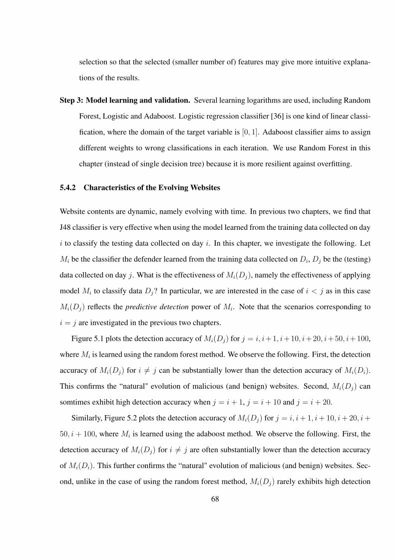
selection so that the selected (smaller number of) features may give more intuitive explana-

tions of the results.

Step 3: Model learning and validation. Several learning logarithms are used, including Random

Forest, Logistic and Adaboost. Logistic regression classifier [36] is one kind of linear classi-

fication, where the domain of the target variable is [0, 1]. Adaboost classifier aims to assign

different weights to wrong classifications in each iteration. We use Random Forest in this

chapter (instead of single decision tree) because it is more resilient against overfitting.

5.4.2 Characteristics of the Evolving Websites

Website contents are dynamic, namely evolving with time. In previous two chapters, we find that

J48 classifier is very effective when using the model learned from the training data collected on day

i to classify the testing data collected on day i. In this chapter, we investigate the following. Let

Mi be the classifier the defender learned from the training data collected on Di, Dj be the (testing)

data collected on day j. What is the effectiveness of Mi(Dj), namely the effectiveness of applying

model Mi to classify data Dj? In particular, we are interested in the case of i < j as in this case

Mi(Dj) reflects the predictive detection power of Mi. Note that the scenarios corresponding to

i = j are investigated in the previous two chapters.

Figure 5.1 plots the detection accuracy of Mi(Dj) for j = i, i+1, i+10, i+20, i+50, i+100,

where Mi is learned using the random forest method. We observe the following. First, the detection

accuracy of Mi(Dj) for i ̸= j can be substantially lower than the detection accuracy of Mi(Di).

This confirms the “natural" evolution of malicious (and benign) websites. Second, Mi(Dj) can

somtimes exhibit high detection accuracy when j = i+ 1, j = i+ 10 and j = i+ 20.

Similarly, Figure 5.2 plots the detection accuracy of Mi(Dj) for j = i, i+1, i+10, i+20, i+

50, i + 100, where Mi is learned using the adaboost method. We observe the following. First, the

detection accuracy of Mi(Dj) for i ̸= j are often substantially lower than the detection accuracy

of Mi(Di). This further confirms the “natural" evolution of malicious (and benign) websites. Sec-

ond, unlike in the case of using the random forest method, Mi(Dj) rarely exhibits high detection

68

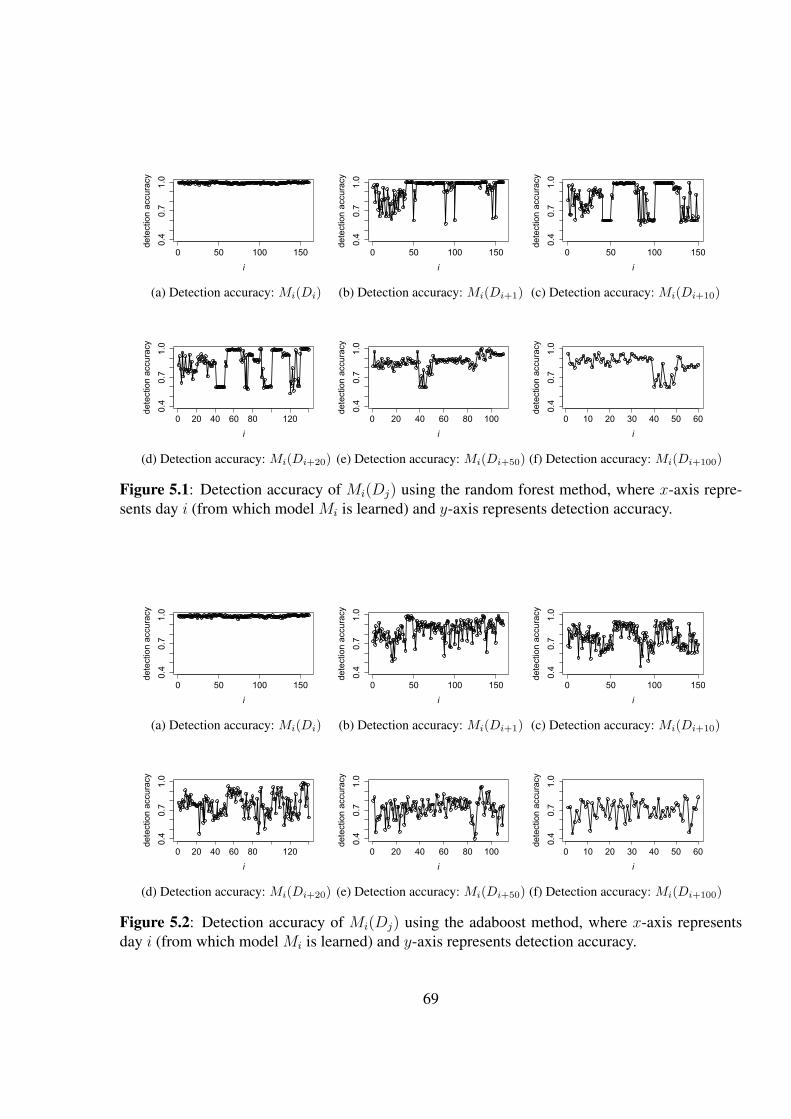
0 50 100 150

0.4

0.7

1.0

i

dete

ctio

n ac

cura

cy

(a) Detection accuracy: Mi(Di)

0 50 100 150

0.4

0.7

1.0

i

dete

ctio

n ac

cura

cy

(b) Detection accuracy: Mi(Di+1)

0 50 100 150

0.4

0.7

1.0

i

dete

ctio

n ac

cura

cy

(c) Detection accuracy: Mi(Di+10)

0 20 40 60 80 120

0.4

0.7

1.0

i

dete

ctio

n ac

cura

cy

(d) Detection accuracy: Mi(Di+20)

0 20 40 60 80 100

0.4

0.7

1.0

i

dete

ctio

n ac

cura

cy

(e) Detection accuracy: Mi(Di+50)

0 10 20 30 40 50 60

0.4

0.7

1.0

i

dete

ctio

n ac

cura

cy

(f) Detection accuracy: Mi(Di+100)

Figure 5.1: Detection accuracy of Mi(Dj) using the random forest method, where x-axis repre-sents day i (from which model Mi is learned) and y-axis represents detection accuracy.

0 50 100 150

0.4

0.7

1.0

i

dete

ctio

n ac

cura

cy

(a) Detection accuracy: Mi(Di)

0 50 100 150

0.4

0.7

1.0

i

dete

ctio

n ac

cura

cy

(b) Detection accuracy: Mi(Di+1)

0 50 100 150

0.4

0.7

1.0

i

dete

ctio

n ac

cura

cy

(c) Detection accuracy: Mi(Di+10)

0 20 40 60 80 120

0.4

0.7

1.0

i

dete

ctio

n ac

cura

cy

(d) Detection accuracy: Mi(Di+20)

0 20 40 60 80 100

0.4

0.7

1.0

i

dete

ctio

n ac

cura

cy

(e) Detection accuracy: Mi(Di+50)

0 10 20 30 40 50 60

0.4

0.7

1.0

i

dete

ctio

n ac

cura

cy

(f) Detection accuracy: Mi(Di+100)

Figure 5.2: Detection accuracy of Mi(Dj) using the adaboost method, where x-axis representsday i (from which model Mi is learned) and y-axis represents detection accuracy.

69

accuracy when j = i+ 1, j = i+ 10 and j = i+ 20.

Explanations of these phenomena will be reported elsewhere.

5.5 Online Learning

Having identified that Mi(Dj) for i < j is substantially less effective than Mi(Di), we need to

identify ways for effectively classify Dj . For this purpose, we propose using online learning.

Vowpal Wabbit is an open source learning software system that includes a series of online ma-

chine learning algorithm. One representative online learning algorithm is logistic regression with

stochastic gradient descent (LRsgd), where model parameters are updated incrementally by the

gradients of feature vectors of benign/malicious URLs. It is worthy mentioning that online ma-

chine learning algorithm scans the training data once — a characteristic that nicely matches the

problem of detecting malicious websites, which dynamically evolve.

The basic idea of online learning is described as follows. Suppose each website is represented

as a feature vector Xi and has a label yi ∈ {0, 1} (i.e., benign or malicious). The online learning

algorithm treats the training data as a stream. For each incoming feature vector X , the online

learning algorithm using the currently classification model, say M , to classify x with label y.

If M ’s classification is correct, there is no need to update M ; otherwise, M is updated toward

correctly classifying X .

Figure 5.3 compare the detection accuracies of random forest classification models obtained

by using or without using online learning algorithm. Specifically, Figure 5.3a shows the detection

accuracy rate for online learning with non-adpative strategy, meaning that the entire history of

training data from D1, . . . , Dj are used for learning M1..j . We observe that the detection accuracy

rate is almost 99.99% at day 0 and drop to 99.40% during the first five days. Then, the detection

accuracy slowly decreases and reaches 98.40% on the 160th day. Figure 5.3b plots the the detection

accuracy rate for online learning with adpative strategy, meaning that only partial history of training

data from Di, . . . , Dj are used for learning Mi..j . We observe that the detection accuracy is actually

higher than that of the non-adaptive strategy. The reason is that the adaptive strategy can disregard

70

0 50 100 1500.98

50.

990

0.99

51.

000

j

dete

ctio

n ac

cura

cy

(a) Non-adaptive online learning strategy: M1..j(Dj)

0 50 100 1500.98

50.

990

0.99

51.

000

j

dete

ctio

n ac

cura

cy

(b) Adaptive online learning strategy: Mi..j(Dj)

Figure 5.3: Detection accuracy of random forest classification models obtained by using onlinelearning algorithm LRsgd with non-adaptive or adpative strategy, where x-axis represents j, y-axisrepresents the detection accuracy rate, M1..j(Dj) means that the model M1..j is learned from theentire history of training data from D1, . . . , Dj (non-adaptive strategy), and Mi..j means that themodel Mi..j is learned from partial history of trainig data from Di, . . . , Dj (adaptive strategy).

data that is “old” enough to cause misclassifications on day j.

5.6 Related Work

Industrial products for detecting malicious websites include McAfee Site Advisor [2] and Google

Safe Browsing [1]. Academic research efforts, which aim at more powerful techniques include

[13–16, 18, 29, 32, 33, 37, 41, 53, 57, 59, 60, 65, 67]. For example, Kim and Leey [57] aim to detect

suspicious URLs embedded in twitter message streams; Invernizzi et al. [29] aim to quickly iden-

tify malicious websites; Xu et al. [65] aim to use both application and network layers information

to detect malicious websites; Gianluca et al. [60] aim to use redirection graphs to detect mali-

cious webpages; Kapravelos et al. [32] aim to automatically detect evasive behavior in malicious

JavaScript. To the best of our knowledge, the present chapter is the first systematic investigation

of the “natural” evolution of malicious websites, and designing countermeasures against them.

71

5.7 Summery

We have showed that malicious websites are evolving. We also have presented online learning

methods, especially adaptive online learning methods, for effectively dealing with evolving mali-

cious websites. Experimental results based on a 160-day dataset shows that the resulting detection

accuracy is very promising. We expect to report more detailed results of this research elsewhere

shortly.

72

Chapter 6: CONCLUSION AND FUTURE WORK

In conclusion, we have investigated three aspects of an important problem: understanding and

detecting malicious websites. While we have made a substantial step towards ultimately solving

the problem, there are many interesting problems that are yet to be tackled before we can achieve

the ultimate goal. Two representative research problems are highlighted below.

First, our current data collection system may not be able to deal with obfuscated JavaScript-

based redirection, which is a challenging open problem [23]. Although our collected data hints

that JavaScript-based redirection is widely used by malicious websites, it appears that JavaScript

obfuscation may not have been widely used because our system can effectively detect the ma-

licious URLs. However, this is not true in general and in the future because the fact — many

malicious websites are using JavaScript-based redirection — does suggest that the attackers will

likely continue using this redirection method, perhaps coupled with obfuscation. It is perhaps

equally important to deal with encrypted web contents using light-weight extensions to the static

analysis. Fortunately, any progress in these directions can be plugged into our system in a modular

fashion. It is possible to enhance our static analysis system by incorporating new techniques such

as those described in [18, 20, 46, 56].

Second, we consider a certain class of adaptive attacks that attempt to evade detection, which

are equally used by both attacker and defender. There could be other classes of adaptive attacks

that may be able to defeat our defense. Our artificial manipulation algorithms for mimicking adap-

tive attacks may or may not be truthful because when the algorithms changes the values of some

application-layer features, some network-layer features may have to be changed correspondingly

so as to make the cross-layer semantics consistent. This is a non-trivial problems because there is

no simple mapping between the application-layer features and the network-layer features. Finally,

our adaptive defense is reminiscent of the studies in robust classifiers [11, 12, 25, 34, 35], which

suggests that our study will spark more investigations on the power and limitation of our defense.

73

BIBLIOGRAPHY

[1] Google safe browing, http://code.google.com/apis/safebrowsing/

developers_guide_v2.html.

[2] http : //en.wikipedia.org/wiki/url_redirection.

[3] iptables 1.4.12.1 www.netfilter.org/projects/iptables.

[4] Know your enemy: Behind the scenes of malicious web servers. http://www.

honeynet.org.

[5] Know your enemy: Malicious web servers. http://www.honeynet.org.

[6] Mcafee. siteadvisor. http://www.siteadvisor.com.

[7] Sophos corporation. security threat report update 07/2008. http://sophos.com/

sophos/docs/eng/papers/sophos-security-report-jul08-srna.pdf.

[8] tcpdump 4.2.0 www.tcpdump.org.

[9] Marco Barreno, Blaine Nelson, Russell Sears, Anthony D. Joseph, and J. D. Tygar. Can

machine learning be secure? In ASIACCS’06, pages 16–25, 2006.

[10] Andras A. Benczur, Karoly Csalogany, Tamas Sarlos, and Mate Uher. Spamrank - fully

automatic link spam detection. In AIRWeb, 2005.

[11] Battista Biggio, Giorgio Fumera, and Fabio Roli. Multiple classifier systems under attack. In

MCS, pages 74–83, 2010.

[12] Leo Breiman. Bagging predictors. Machine Learning, pages 123–140, 1996.

[13] Davide Canali and Davide Balzarotti. Behind the scenes of online attacks: an analysis of

exploitation behaviors on the web. In NDSS ’13.

74

[14] Davide Canali, Marco Cova, Giovanni Vigna, and Christopher Kruegel. Prophiler: a fast

filter for the large-scale detection of malicious web pages. Proc. WWW’11, pages 197–206.

ACM, 2011.

[15] Kevin Zhijie Chen, Guofei Gu, Jose Nazario, Xinhui Han, and Jianwei Zhuge. WebPatrol:

Automated collection and replay of web-based malware scenarios. In ASIACCS’11), 2011.

[16] Hyunsang Choi, Bin B. Zhu, and Heejo Lee. Detecting malicious web links and identifying

their attack types. In WebApps’11, pages 11–11, 2011.

[17] Corinna Cortes and Vladimir Vapnik. Support-vector networks. In Machine Learning, pages

273–297, 1995.

[18] Marco Cova, Christopher Kruegel, and Giovanni Vigna. Detection and analysis of drive-by-

download attacks and malicious javascript code. In WWW10, 2010.

[19] Thomas M. Cover and Joy A. Thomas. Elements of information theory. Wiley-Interscience,

New York, NY, USA, 1991.

[20] Charlie Curtsinger, Benjamin Livshits, Benjamin Zorn, and Christian Seifert. Zozzle: fast

and precise in-browser javascript malware detection. In USENIX Security, 2011.

[21] Nilesh Dalvi, Pedro Domingos, Mausam, Sumit Sanghai, and Deepak Verma. Adversarial

classification. In KDD’04, pages 99–108, 2004.

[22] Andreas Dewald, Thorsten Holz, and Felix C. Freiling. Adsandbox: sandboxing javascript to

fight malicious websites. In SAC’10, pages 1859–1864, 2010.

[23] Ben Feinstein and Daniel Peck. Caffeine monkey: Automated collection, detection and anal-

ysis of malicious javascript. In DEFCON 15, 2007.

[24] Sujata Garera, Niels Provos, Monica Chew, and Aviel D. Rubin. A framework for detection

and measurement of phishing attacks. In WORM’07, pages 1–8, 2007.

75

[25] Amir Globerson and Sam T. Roweis. Nightmare at test time: robust learning by feature

deletion. In ICML, pages 353–360, 2006.

[26] M. A. Hall. Correlation-based Feature Subset Selection for Machine Learning. PhD thesis,

University of Waikato, Hamilton, New Zealand, 1998.

[27] Mark Hall, Eibe Frank, Geoffrey Holmes, Bernhard Pfahringer, Peter Reutemann, and Ian H.

Witten. The weka data mining software: an update. SIGKDD Explor. Newsl., pages 10–18,

2009.

[28] Yung-Tsung Hou, Yimeng Chang, Tsuhan Chen, Chi-Sung Laih, and Chia-Mei Chen. Mali-

cious web content detection by machine learning. Expert Syst. Appl., pages 55–60, January

2010.

[29] Luca Invernizzi, Stefano Benvenuti, Marco Cova, Paolo Milani Comparetti, Christopher

Kruegel, and Giovanni Vigna. Evilseed: A guided approach to finding malicious web pages.

In Proceedings of the 2012 IEEE Symposium on Security and Privacy, SP ’12, pages 428–

442.

[30] G. H. John and P. Langley. Estimating continuous distributions in Bayesian classifiers. UAI,

pages 338–345, 1995.

[31] A. Kapravelos, M. Cova, C. Kruegel, and G. Vigna. Escape from monkey island: Evading

high-interaction honeyclients. In DIMVA’11, 2011.

[32] A. Kapravelos, Y. Shoshitaishvili, M. Cova, C. Kruegel, and G. Vigna. Revolver: An au-

tomated approach to the detection of evasive web-based malware. In Proceedings of the

USENIX Security Symposium, 2013.

[33] Alexandros Kapravelos, Marco Cova, Christopher Kruegel, and Giovanni Vigna. Escape from

monkey island: Evading high-interaction honeyclients. In DIMVA, pages 124–143, 2011.

76

[34] Josef Kittler, Mohamad Hatef, Robert P. W. Duin, and Jiri Matas. On combining classifiers.

TPAMI, pages 226–239, 1998.

[35] Aleksander Kolcz and Choon Hui Teo. Feature weighting for improved classifier robustness.

In CEAS, 2009.

[36] S. le Cessie and J.C. van Houwelingen. Ridge estimators in logistic regression. Applied

Statistics, pages 191–201, 1992.

[37] Guanhua Yan Lei Liu, Xinwen Zhang and Songqing Chen. Chrome extensions: Threat anal-

ysis and countermeasures. In NDSS ’13.

[38] Daniel Lowd and Christopher Meek. Adversarial learning. In KDD’05, pages 641–647, 2005.

[39] Justin Ma, Lawrence K. Saul, Stefan Savage, and Geoffrey M. Voelker. Beyond blacklists:

learning to detect malicious web sites from suspicious urls. In KDD’09, pages 1245–1254,

2009.

[40] Justin Ma, Lawrence K. Saul, Stefan Savage, and Geoffrey M. Voelker. Identifying suspicious

urls: an application of large-scale online learning. In ICML’09, pages 681–688, 2009.

[41] Tilman Frosch Mario Heiderich and Thorsten Holz. Iceshield: Detection and mitigation of

malicious websites with a frozen dom. In RAID’11, 2011.

[42] Jose Nazario. Phoneyc: A virtual client honeypot, 2009.

[43] Blaine Nelson, Benjamin I. P. Rubinstein, Ling Huang, Anthony D. Joseph, and J. D. Tygar.

Classifier evasion: models and open problems. In ECML PKDD 2011, pages 92–98, 2011.

[44] James Newsome, Brad Karp, and Dawn Song. Paragraph: Thwarting signature learning by

training maliciously. In RAID06, 2006.

[45] Yuan Niu, Yi min Wang, Hao Chen, Ming Ma, and Francis Hsu. A quantitative study of

forum spamming using contextbased analysis. In NDSS, 2007.

77

[46] W Palant. Javascript deobfuscator 1.5.8. https://addons.mozilla.org/en-US/

firefox/addon/javascript-deobfuscator/, 2010.

[47] Roberto Perdisci, David Dagon, Wenke Lee, Prahlad Fogla, and Monirul Sharif. Misleading

worm signature generators using deliberate noise injection. In Proc. S&P’06, 2006.

[48] Roberto Perdisci, Guofei Gu, and Wenke Lee. Using an ensemble of one-class svm classifiers

to harden payload-based anomaly detection systems. In ICDM, pages 488–498, 2006.

[49] J. Platt. Fast training of support vector machines using sequential minimal optimization. In

Advances in Kernel Methods – Support Vector Learning, pages 42–65. 1998.

[50] Niels Provos, Panayiotis Mavrommatis, Moheeb Abu Rajab, and Fabian Monrose. All your

iframes point to us. In USENIX Security, 2008.

[51] Zhiyun Qian, Zhuoqing Morley Mao, Yinglian Xie, and Fang Yu. On network-level clusters

for spam detection. In NDSS, 2010.

[52] Ross Quinlan. C4.5: Programs for Machine Learning. San Mateo, CA, 1993.

[53] Moheeb Rajab, Lucas Ballard, Nav Jagpal, Panayiotis Mavrommatis, Daisuke Nojiri, Niels

Provos, and Ludwig Schmidt. Trends in circumventing web-malware detection. Technical

report, Google, 2011.

[54] Konrad Rieck, Tammo Krueger, and Andreas Dewald. Cujo: efficient detection and preven-

tion of drive-by-download attacks. In ACSAC’10, pages 31–39, 2010.

[55] Benjamin I.P. Rubinstein, Blaine Nelson, Ling Huang, Anthony D. Joseph, Shing-hon Lau,

Satish Rao, Nina Taft, and J. D. Tygar. Antidote: understanding and defending against poi-

soning of anomaly detectors. In IMC’09, pages 1–14, 2009.

[56] Chenette S. The ultimate deobfuscator. http://securitylabs.websense.com/

content/Blogs/3198.aspx.

78

[57] Jong Kim Sangho Leey. Warningbird: Detecting suspicious urls in twitter stream. In NDSS

’12.

[58] Christian Seifert and Ramon Steenson. Capture - Honeypot Client (Capture-HPC). https:

//projects.honeynet.org/capture-hpc, 2006.

[59] Vitaly Shmatikov Sooel Son. The postman always rings twice: Attacking and defending

postmessage in html5websites. In NDSS ’13, NDSS ’13, 2013.

[60] Gianluca Stringhini, Christopher Kruegel, and Giovanni Vigna. Shady paths: leveraging

surfing crowds to detect malicious web pages. CCS ’13, pages 133–144.

[61] Kurt Thomas, Chris Grier, Justin Ma, Vern Paxson, and Dawn Song. Design and Evaluation

of a Real-Time URL Spam Filtering Service. In Proc. IEEE S&P’11, 2011.

[62] Shobha Venkataraman, Avrim Blum, and Dawn Song. Limits of learning-based signature

generation with adversaries. In NDSS, 2008.

[63] Yi-Min Wang, Doug Beck, Xuxian Jiang, and Roussi Roussev. Automated web patrol with

strider honeymonkeys: Finding web sites that exploit browser vulnerabilities. In NDSS’06,

2006.

[64] Colin Whittaker, Brian Ryner, and Marria Nazif. Large-scale automatic classification of

phishing pages. In NDSS, 2010.

[65] Li Xu, Zhenxin Zhan, Shouhuai Xu, and Keying Ye. Cross-layer detection of malicious

websites. In CODASPY, pages 141–152, 2013.

[66] Wei Xu, Fangfang Zhang, and Sencun Zhu. Jstill: mostly static detection of obfuscated ma-

licious javascript code. In Proceedings of the third ACM conference on Data and application

security and privacy, CODASPY ’13, pages 117–128, 2013.

[67] Junjie Zhang, Christian Seifert, Jack W. Stokes, and Wenke Lee. Arrow: Generating signa-

tures to detect drive-by downloads. In WWW, pages 187–196, 2011.

79

VITA

Li Xu received his B.S. degree and M.SC. degree from China. He started his Ph.D. study at

University of Texas at San Antonio from September 2008.