detecting trends in the annual maximum discharges in the...
TRANSCRIPT

DOI: 10.2478/aslh-2014-0010 Acta Silv. Lign. Hung., Vol. 10, Nr. 2 (2014) 133–144
Detecting Trends in the Annual Maximum Discharges
in the Vah River Basin, Slovakia
Katarína JENEIOVÁa*
– Silvia KOHNOVÁa – Miroslav SABO
b
a
Department of Land and Water Resources Management, Faculty of Civil Engineering,
Slovak University of Technology, Bratislava, Slovakia b
Department of Mathematics and Descriptive Geometry, Faculty of Civil Engineering,
Slovak University of Technology, Bratislava, Slovakia
Abstract – A number of floods have been observed in the Slovak Republic in recent years, thereby
raising awareness of and concern about flood risks. The paper focuses on the trend detection in the
annual maximum discharge series in the Vah River basin located in Slovak Republic. Analysis was
performed on data obtained from 59 gauging stations with minimum lengths of the observations from
40 years to 109 years. Homogeneity of the time series was tested by Alexandersson test for single shift
at 5% level of significance. The Mann-Kendall trend test and its correction for autocorrelated data by
Hamed and Rao (1998) were used to analyse the significance of detected changes in discharges. The
series were analysed at different lengths of 40, 50, 60 years and whole observation period. Statistically
significant rising and decreasing trends in the annual maximum discharge series were found in
different regions of the Vah River catchments.
maximum annual discharges / homogeneity / Mann-Kendall trend test
Kivonat – Az évi maximális vízhozamok trend elemzése a Vág (Vah) vízgyűjtőjében, Szlovákiában.
Az árhullámok száma igen jelentős napjainkban a Szlovák Köztársaságban, ezért egyre nagyobb az
igény az árvízi kockázat elemzésekre. Jelen tanulmány az évi maximális vízhozamok tendenciájának
elemzésére koncentrál a Szlovák Köztársaságban található Vág vízgyűjtőjében. Az elemzés alapját 59
vízmérce állomás idősoros adatai adták, amely idősorok hossza 40-től 109 évig változott. Az idősorok
homogenitása Alexandersson tesztel lett értékelve 5%-os megbízhatósági szinten. A vízhozamban
bekövetkező változások szignifikanciájának elemzésére Mann-Kendall tesztet, illetve annak Hamed és
Rao (1998) által továbbfejlesztett, autokorrelált adatokra értelmezett változatát használtuk. Az idő-
sorokat egységes hosszakban, 40, 50, 60 év, és a teljes észlelési időszakra vonatkozóan is értékeltük.
Az eredmények alapján statisztikailag szignifikáns emelkedő és csökkenő trendek is kimutathatók
voltak a maximális évi vízhozamokban a Vág vízgyűjtőjének különböző régióiban.
évi maximális vízhozam / homogenitás / Mann-Kandall trend teszt
* Corresponding author: [email protected], Radlinského 11, 813 68 BRATISLAVA, Slovakia

Jeneiová, K. et al.
Acta Silv. Lign. Hung. 10 (2), 2014
134
1 INTRODUCTION
A number of floods have been observed around Europe in recent decades, which have raised
awareness of and concerns about flood risks. The observation and detection of changes in
long-term hydrological time series is important for scientific and practical reasons, especially
when designing water management structures.
There is a need to understand hydrological processes on small and also large temporal
and spatial scales, land-atmosphere interactions, land use and climate change impacts
(Szolgay, 2011). Further Blöschl et al. (2007) discuss the scales of climate variability and
land cover change impact on flooding. In the note they debate, that climate change impact is
likely to occur at large scales and to be consistent in both small and large catchments and
regions, while land cover change is usually a local phenomenon, which effects are decreasing
at larger spatial scale. Therefore the major driving forces behind hydrological phenomenons
can vary depending on the factor and spatial scale
Many studies dealing with analyses of trends concerning floods have been published;
many of them have found decreasing or increasing trends in their magnitudes and
occurrences, and many have also found no changes (Strupczewski et al. 2001, Xiong – Guo
2004, Delgado et al. 2010, Armstrong et al. 2012, Rougé et al. 2013). The Mann-Kendall test
(Kendall 1975, Kliment et al. 2011, Armstrong, 2012) is widely used in engineering
hydrology to detect trends. When the data do not follow the normal distribution or are
autocorrelated, authors have suggested the use of test corrections (Douglas et al. 2000, Burn –
Hag Elnur 2001, Zhang et al. 2001, Yue et al. 2002, Lang 2012, Seoane – Lopez 2007,
Danneberg 2012).
Strupczewski et al. (2001) investigated trends in 70-year-long observations of the annual
maximum flows of Polish rivers. A decreasing tendency in the mean and standard deviations
of annual peak flows was found with the use of the maximum likelihood method for
estimating parameters and the Akaike Information Criterion for identification of an optimum
model. Xiong and Guo (2004) tested maximum annual discharge series, including the mean
annual maximum of the Yangtze River during a 120-year-long time period. No significant
trend at the 5% significance level was found by the use of the Mann-Kendall test and
Spearman’s rho at the tested station. Delgado et al. (2010) examined over 70-year-long annual
maximum discharge series from 4 gauging stations in the Mekong river in Southeast Asia
with use of Mann Kendal test, ordinary least squares with resampling and non-stationary
generalised extreme value functions. The results of the study pointed out increasing likelihood
of extreme floods during the last half of century. They also concluded that the absence of
detected positive trends was a result of methodological misconception due to simplistic
models.
Armstrong et al. (2012) analysed peak over threshold data with a recorded average period
of 71 years. An increasing trend was found with the use of the Mann-Kendall trend test in
22 stations out of the 23 investigated, and a hydroclimatic shift towards a rising number of flood
occurrences was found. Rougé et al. (2013) studied trend and step-change detection methods
in hydrological time series (rainfall, river flows) and applied a combined Mann-Kendall and
Pettitt test (1979) on 1217 data sets in the United States during the years 1910–2009.
In Slovakia, a long-term annual time series was investigated by Pekarova et al. (2008). In
a IHP UNESCO report (Pekarova et al., 2008), daily discharges of the Danube River from
1976-2005 were analysed, and a rising tendency was detected, but no change was found in the
annual and monthly time series. The Mann-Kendall trend test was used in Tegelhoffova
(2012) to detect trends in the average annual and monthly discharges in Slovak rivers.
However, no thoughtful trend analysis of annual maximum discharges in Slovak catchments
has been provided.

Trends in the annual maximum discharges, Vah Basin
Acta Silv. Lign. Hung. 10 (2), 2014
135
This paper focuses on a time series analysis and significance assessment of trends
detected in annual maximum discharge series in the Vah River catchment in the Slovak
Republic and the lessons learned concerning the occurrence of extreme discharges in the Vah
River catchments. The paper is organised as follows: methodology, input data description,
results and discussion, and conclusions.
2 METHODS
In engineering hydrology, time series analysis usually operates under the assumption of
homogeneity, stationarity and independence of time series. Homogeneity in the time series
can be tested by Alexandersson test (Alexandersson – Moberg 1997), which is able to detect
abrupt changes in analysed data set. We used Alexandersson test (Standard normal
homogeneity test, SNHT) for single shift programmed in AnClim software (Stepanek 2007).
The significance of monotonic linear trend present in the time series is possible to assess
by Theil (1950) and Sen (1968) slope defined as:
β = Median (
Xj−Xl
j−l)∀ l < 𝑗, (1)
where β is the estimate of slope of the trend and xj is value of observation from j= 1...l.
Positive value of β reveals increasing trend, negative value is sign of decreasing trend.
Changes in a trend can be detected by a rank-based, non-parametric Mann-Kendall trend
test for monotonic trends (WMO 2000).
The test statistic S equals to (Yue et al. 2012):
𝑆 = ∑ ∑ 𝑠𝑖𝑔𝑛(𝑥𝑗 − 𝑥𝑘)
𝑛𝑗=𝑘+1
𝑛−1𝑘=1 , (2)
where xj are the values of the data; n is the length of the time series and
Sign(xj – xk) = 1, if xj – xk > 0
= 0, if xj – xk = 0 (3)
= -1, if xj – xk < 0.
In case the time series has n≥8, the statistic S has and almost normal distribution, and its
variance is computed as:
𝑉𝐴𝑅(𝑆) =1
18[𝑛(𝑛 − 1)(2𝑛 + 5) − ∑ 𝑡𝑝(𝑡𝑝 − 1)(2𝑡𝑝 + 5)
𝑔𝑝=1 ] , (4)
where g is the number of tied groups, and tp is the amount of data with the same value in the
group p=1...g.
The normalised test statistic Z:
Z =
{
𝑆−1
√𝑉𝑎𝑟(𝑆) for S > 0
0 for S = 0𝑆+1
√𝑉𝑎𝑟(𝑆)for S < 0
(5)
If the normalised test statistic Z is equal to zero, the data are normally distributed, and the
positive values of Z mean a rising trend and negative a decreasing trend (Yue et al. 2012).

Jeneiová, K. et al.
Acta Silv. Lign. Hung. 10 (2), 2014
136
The p-value is computed as:
𝑝 = 0,5 − 𝛷(|𝑍|) 𝑘𝑑𝑒 𝛷(|𝑍|) = 1
√2𝜋∫ 𝑒
𝑡2
2 𝑑𝑡|𝑍|
0. (6)
If the data are not independent a correction of the MK trend test should be used.
Autocorrelation can influence the results of the analysis (Lang 2012, Yue et al. 2002). Hamed
and Rao (HR) (1998) correction addresses the issue of autocorrelation in the time series. The
modified MK equation for any variance is:
V*(S) = VAR(S)n
n*, (7)
where VAR(S) is a variance from the original MK test (4); n is the length of the time series;
n* is the effective number of observations and
𝑛
𝑛∗ is the correction factor in the case of
autocorrelation in the sample.
The modified MK statistic:
𝑍∗ =
{
𝑆−1
√𝑉∗(𝑆) pre S > 0
0 pre S = 0𝑆+1
√𝑉∗(𝑆)pre S < 0
. (8)
The correction factor can be calculated as:
𝑛
𝑛∗= 1 +
2
𝑛(𝑛−1)(𝑛−2)∑ (𝑛 − 𝑘)(𝑛 − 𝑘 − 1)(𝑛 − 𝑘 − 2)𝑟𝑘
𝑅𝑛−1𝑗=1 , (9)
where 𝑟𝑘𝑅 is the autocorrelation function of the ranks of the observations. It can also be
calculated by the equation by Salas et al. (1980):
𝑟𝑘 =1
𝑛−𝑘∑ (𝑋𝑡−𝐸(𝑋𝑡))(𝑋𝑡+𝑘−𝐸(𝑋𝑡))𝑛−𝑘𝑡=11
𝑛∑ (𝑋𝑡−𝐸(𝑋𝑡))2𝑛𝑡=1
, (10)
where
𝐸(𝑋𝑡) =1
𝑛∑ 𝑋𝑡𝑛𝑡=1 , (11)
where rk is the correction factor for the data Xt; E(Xt) is the average of the input data.
Hamed and Rao (1998) also suggest using only statistically significant values of rk,
because other values have a negative influence on the values of variance S.
The null hypothesis of the MK and HR tests states that there is no perceptible trend in the
sample data. If the resulting p-value is lower than level of significance, then we can reject the
null hypothesis (Diermanse et al. 2010).
The Sen’s slope and trend analysis tests were programmed and performed in the R free
software programming language using the fume and Kendall packages (McLeod 2011,
Santahter Meteorology Group 2012, R Core Team 2013).
Trends in the annual maximum discharges, Vah Basin
Acta Silv. Lign. Hung. 10 (2), 2014
137
3 INPUT DATA
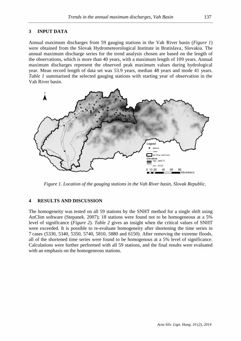
Annual maximum discharges from 59 gauging stations in the Vah River basin (Figure 1)
were obtained from the Slovak Hydrometeorological Institute in Bratislava, Slovakia. The
annual maximum discharge series for the trend analysis chosen are based on the length of
the observations, which is more than 40 years, with a maximum length of 109 years. Annual
maximum discharges represent the observed peak maximum values during hydrological
year. Mean record length of data set was 53.9 years, median 48 years and mode 41 years.
Table 1 summarised the selected gauging stations with starting year of observation in the
Vah River basin.
Figure 1. Location of the gauging stations in the Vah River basin, Slovak Republic.
4 RESULTS AND DISCUSSION
The homogeneity was tested on all 59 stations by the SNHT method for a single shift using
AnClim software (Stepanek. 2007); 18 stations were found not to be homogeneous at a 5%
level of significance (Figure 2). Table 2 gives an insight when the critical values of SNHT
were exceeded. It is possible to re-evaluate homogeneity after shortening the time series in
7 cases (5330, 5340, 5350, 5740, 5810, 5880 and 6150). After removing the extreme floods,
all of the shortened time series were found to be homogenous at a 5% level of significance.
Calculations were further performed with all 59 stations, and the final results were evaluated
with an emphasis on the homogeneous stations.

Jeneiová, K. et al.
Acta Silv. Lign. Hung. 10 (2), 2014
138
Table 1. List of selected gauging stations in the Vah River basin
Station
number
Name of the
station Catchment
Starting
year of
observations
Station
number
Name of the
station Catchment
Starting
year of
observations
5300 Liptovská
Teplička
Čierny Váh 1967 5890 Turany Čiernik 1970
5310 Čierny Váh Ipoltica 1961 5930 Turček Turiec 1967
5311 Čierny Váh Čierny Váh 1921 5970 Turčianske
Teplice
Teplica 1963
5330 Východná Biely Váh 1923 5980 Háj Somolan 1969
5336 Malužiná Boca 1970 6030 Brčna Sloviansky P. 1969
5340 Kráľova Lehota Boca 1931 6070 Blatnica Gaderský P. 1969
5350 Kráľova Lehota Hybica 1965 6110 Necpaly Necpalsky P. 1970
5370 Liptovský
Hrádok
Váh 1951 6130 Martin Turiec 1937
5400 Podbanské Belá 1928 6140 Martin Pivovarský P. 1969
5460 Račková Dolina Račkový P. 1963 6150 Stráža Varínka 1957
5480 Liptovský
Hrádok
Belá 1965 6190 Zborov
N/Bystricou
Bystrica 1949
5520 Liptovský Ján Štiavnica 1963 6200 Kysucké Nové
Mesto
Kysuca 1931
5530 Žiarska Dolina Smrečianka 1963 6230 Rajecká Lesná Lesňanka 1968
5540 Iľanovo Iľanovianka 1969 6240 Šuja Rajčianka 1968
5550 Liptovský
Mikuláš
Váh 1932 6260 Rajec Čierňanka 1968
5590 Demänová Demänovka 1969 6290 Rajecke Teplice Kunedradsky
P.
1969
5650 Prosiek Prosiečanka 1969 6300 Poluvsie Rajčianka 1930
5660 Horáreň Hluché Paludźanka 1970 6330 Lietava, Majer Lietavka 1969
5680 Liptovský Sv.
Kríž
Paludźanka 1969 6340 Závodie Rajčianka 1967
5720 Liptovské
Vlachy
Kľačianka 1962 6360 Bytča Petrovička 1961
5730 Partizánska
Ľupča
Ľupčianka 1961 6370 Prečín Domanižanka 1969
5740 Podsuchá Revúca 1929 6380 Považská
Bystrica
Domanižanka 1961
5780 Hubová Váh 1921 6390 Vydrná Petrinovec 1961
5790 Ľubochňa Ľubochnianka 1959 6400 Dohňany Biela Voda 1961
5800 Lokca Biela Orava 1951 6420 Visolaje Pružinka 1961
5810 Oravská Jasenica Veselianka 1951 6450 Horné Srnie Vlára 1961
5820 Zubrohlava Polhoranka 1951 6460 Trenčianske
Teplice
Teplička 1962
5840 Trstená Oravica 1961 6470 Čachtice Jablonka 1961
5870 Párnica Zázrivka 1963 6480 Šaľa Váh 1901
5880 Dierová Orava 1931

Trends in the annual maximum discharges, Vah Basin
Acta Silv. Lign. Hung. 10 (2), 2014
139
Table 2. Non- homogeneous stations at a 95% level of significance according to the SNHT
test (To is the highest computed value of SNHT test statistics for the station;
homogeneous stations after the removal of the extreme floods are marked in bold)
Station Start year of
observation Statistic To
Critical values
(Khaliq and
Ouarda, 2007)
Critical value
exceeded
(Years)
5330 1923 14.272 9.047 1940–1957
5340 1931 9.303 8.951 1931
5350 1965 9.015 8.331 1965
5520 1963 8.711 8.382 1985–87
5650 1969 16.409 8.214 2009
5720 1962 17.566 8.382 1972–1984
5740 1929 15.753 8.976 1938–1963
5780 1921 19.802 9.067 1958–1995
5810 1951 9.079 8.647 1960
5840 1961 21.673 8.432 1999–2008
5870 1963 10.691 8.382 1993–1995
5880 1931 16.197 8.951 1940–1967
5890 1970 10.887 8.151 1979–1984
5970 1963 10.479 8.382 2009
6150 1957 11.616 8.524 1958, 1960
6360 1961 21.434 8.432 1995–2007
6390 1961 10.089 8.432 1973
6470 1961 15.362 8.432 2000–2005
Figure 2. Map with locations and station number of homogeneous and nonhomogeneous
stations at a 95% level of significance in the Vah River basin
Jeneiová, K. et al.
Acta Silv. Lign. Hung. 10 (2), 2014
140
For each of the 59 stations, the positive or negative direction of the trend was calculated
by Sen’s slope. The trend detected was positive in 27 cases and negative in 32 cases.
The MK and HR tests were applied to the discharge series in the Vah River catchment to
assess the significance of the trend for different observation lengths: 40 years from 1970 to
2010; 50 years from 1960 to 2010; 60 years from 1950 to 2010; and the whole period of time
observed at all the stations (40 years was the shortest and 109 years was the longest period).
In the case of the autocorrelation in the time series, the test results of the MK and HR tests
differ; therefore, there is a need to use the corrected HR test. The results were evaluated at the
significance levels of 5, 10 and 20% (Table 3).
Table 3. Number of catchments at the levels of significance of 5, 10 and 20% by the MK and
HR tests at different lengths of the observations
Number of gauging stations 59 20 14 59
Time period (years) 40 50 60 40–109
Trend test MK HR MK HR MK HR MK HR
Sig
nif
ican
ce
level
(num
ber
of
stat
ions)
5% 8 12 3 3 3 2 16 15
10% 17 16 4 3 3 3 22 19
20% 24 23 5 5 4 4 25 24
The null hypothesis (no trend in the time series) could not be rejected at the 20%
significance level in 24 cases for the MK and 23 cases for the HR tests in the 40-year-long
time period, in 5 cases for both the MK and HR in the 50-year-long time period, in 4 cases
for both the MK and HR in the 60-year-long time period; and in 25 cases for the MK and
in 24 cases for the HR for the whole time series. At the 10% level of significance, a trend
was observed in 17 cases for the MK test and 16 for the HR test in the 40 year-long-
period, 4 cases for the MK and 3 cases for the HR in the 50-year-long period, 3 cases for
both the MK and HR during the 60-year-long-period; and in 22 cases for the MK and in
19 cases for the HR for the whole available time series. A trend at the 5% significance
level was found in 8 cases for the MK and in 12 cases for the HR tests in the 40-year-long
time period, in 3 cases for both the MK and HR in the 50-year-long time period, in 3 cases
for the MK and in 2 cases for the HR in the 60-year-long time period, and in 16 cases for
the MK and in 15 cases for the HR for the whole available time series.
Due to the autocorrelation present in the time series, the results for the MK trend test
and HR test differ; therefore, the HR results were chosen for further analysis. The results
of the HR trend test are presented in Figure 3, which describes the spatial distribution of
rising or decreasing trends detected with significance at the 5%, 10% and 20% levels. The
results of the 40 years of observations and the whole observed time period suggest the
centralisation of a significant rising trend in the upper parts of the catchment and a
decreasing trend in the lower parts of the upper Vah River basin. For the length of
50 years, the number of stations decreased to 20, and a significant trend was found in
5 stations, with a centralised rising trend present in the upper parts of the Vah River
catchment. Sixty years of observations were available for 14 stations with a statistically
significant trend in 4 stations with no clear spatial pattern.

Trends in the annual maximum discharges, Vah Basin
Acta Silv. Lign. Hung. 10 (2), 2014
141
40 years 50 years
60 years Whole time period
Figure 3. The results of the testing at the 5-, 10- and 20-% significance level
Subsequently, we took a closer look at 13 stations with observation periods longer than
60 years (Table 3). In the last column of Table 4, it can be seen that in stations with lengths of
observations longer than 60 years, a statistically significant decreasing trend was found
(Podsuchá, Hubová, Dierová, Martin, Zborov nad Bystricou and Šaľa); three of those time
series (Podsuchá, Hubová and Dierová) were found to be non homogeneous by the SNHT
test. A statistically significant rising trend was found at the Východná station, no trend was
detected at the rest of the stations.

Jeneiová, K. et al.
Acta Silv. Lign. Hung. 10 (2), 2014
142
Table 4. Results of the significance analysis for catchments with 60 or more years of
observations (the p-value is displayed in %); bold – statistically significant values
for a rising trend, bold-italic – statistically significant values for a decreasing trend
Station Name Homogeneity Years of
observation Sen’s slope
P-value (%)
40y 50y 60y whole
5311 Čierny Váh Yes 89 increasing 69.42 70.87 39.38 52.15
5330 Východná No 87 increasing 93.73 38.04 15.23 0
5340 Kráľova Lehota No 79 decreasing 24.73 19.16 2.67 30.09
5400 Podbanské Yes 82 decreasing 81.35 94.17 65.41 66.24
5550 Liptovský Mikuláš Yes 62 decreasing 26.09 58.9 65.57 36.57
5740 Podsuchá No 81 decreasing 46.53 40.28 49.36 0.77
5780 Hubová No 89 decreasing 0.53 0.3 0.03 0
5880 Dierová No 79 decreasing 87.5 66.92 25.79 0
6130 Martin Yes 73 decreasing 86.62 53.7 62.02 3.53
6190 Zborov nad Bystricou Yes 61 decreasing 6.74 0.17 7.42 7.15
6200 Kysucké Nové Mesto Yes 79 decreasing 94.26 27.58 85.26 47.61
6300 Poluvšie Yes 80 increasing 62.11 25.89 96.24 98.39
6480 Šaľa Yes 109 decreasing 62.91 32.97 27.07 6.48
5 CONCLUSIONS
The paper was focused on an analysis of changes in annual maximum discharges in the Vah
River basin by the use of trend significance analysis methods. The quality of the data set was
tested by the Alexandersson SNHT test. The MK and HR trend tests were applied to different
observation lengths – 40, 50, 60 and more than 60-year-long time series obtained from
59 gauging stations in the Vah River catchment.
A more detailed analysis of 13 stations with the longest periods of observations revealed
that with a prolonged length of observation, the possibility of detecting a statistically
significant trend increases. The short length of the time series (in some cases, 40 years) may
have influenced the possibility of detecting a significant trend in the Vah River catchment, in
that any prolongation of a time series observed can significantly influence the detection of a
significant trend at the 5% significance level (Diermanse et al. 2010). When we also took into
consideration the homogeneity analysis results of the SNHT method, a statistically significant
decreasing trend was present at the Dierová, Martin, Zborov nad Bystricou and Šala stations.
Finally, we can conclude that a significant rising trend was detected in the upper part of
the catchment, mainly in the east Tatra Mountain region and a decreasing trend in the lower
part of the upper Vah River basin. These results can help when mapping flood risk areas and
developing river basin management plans in the Vah River basin.
Acknowledgement: This work was supported by the Slovak Research and Development
Agency under Contract Nos. 0015-10. The support is gratefully acknowledged.

Trends in the annual maximum discharges, Vah Basin
Acta Silv. Lign. Hung. 10 (2), 2014
143
REFERENCES
ALEXANDERSSON, H. – MOBERG, A. (1997): Homogenization of Swedish temperature data. Part I:
Homogeneity test for linear trends. Int. J. Climatol. (17): 25–34.
ARMSTRONG, W.H. – COLLINS, M.J. – SNYDER, N.P. (2012): Increased Frequency of Low-Magnitude
Floods in New England, Journal of The American Water Resources Association. 48 (2): 306–320.
BLÖSCHL, G. – ARDOIN-BARDIN, S. – BONELL, M. – DORNINGER, M. – GOODRICH, D. – GUTKNECHT,
D. – MATAMOROS, D. – MERZ, B. – SHAND, P. – SZOLGAY, J. (2007): At what scales do climate
variability and land cover change impact on flooding and low flows? (Note). 21 (9): 1241–1247.
BURN, D.H. – HAG ELNUR, M.A. (2002): Detection of Hydrologic Trends and Variability, Journal of
Hydrology (255): 107–122.
DANNEBERG, J. (2012): Changes in Runoff Time Series in Thuringia, Germany, Mann-Kendall Trend
Test and Extreme Value Analysis, Adv. Geosci. (31): 49–56.
DELGADO, J. M. – APEL, H. – MERZ, B. (2010): Flood trends and variability in the Mekong river,
Hydrol. Earth Syst. Sci. (14): 407–418.
DIERMANSE, F.L.M. – KWADIJK, J.C.J. – BECKERS, J.V.L. – CREBAS, J.I. (2010): Statistical Trend
Analysis of Annual Maximum Discharges of the Rhine And Meuse Rivers. BHS Third
International Symposium, Managing Consequences of a Changing Global Environment,
Newcastle 2010, UK
DOUGLAS, E.M. – VOGEL, R.M. – KROLL, C.N. (2000): Trends in Floods and Low Flows in the United
States: Inpact of Spatial Correlation, Journal of Hydrology. 240 (1–2): 90–105.
HAMED, K.H. – RAO, A.R. (1998): A Modifed Mann-Kendall Trend Test for Autocorrelated Data,
Journal of Hydrology. (204): 182–196.
KENDALL, M.G. (1975) Rank Correlation Methods. London: Griffin.
KHALIQ, M. N. – OUARDA, T. B. M. J. (2007): Short Communication: On the critical values of the
standard normal homogeneity test (SNHT), Int. J. Climatol. 27: 681–687
KLIMENT, Z. – MATOUŠKOVÁ, M. – LEDVINKA, O. – KRÁLOVEC, V. (2011): Hodnocení Trend Trendů
v Hydro-Klimatických Řadách Napříkladu Vybraných Horských Povodí (Evaluating of trends in
hydroclimate time series, for example mountain streams). Středová, H., Rožnovský, J.,
Litschmann, T. (Eds): Mikroklima a Mezoklima Krajinných Struktur a Antropogenních Prostředí
(Microclimate and mezoclimate of landscapes and antropogene landscapes). Skalní Mlýn, 2. –
4.2. 2011.
LANG, M. (2012): Statistical Methods for Detection of Changes Within Hydrological Series. Floodfreq
Action, Subgroup WG4-3 “Trend Analysis of Hydrological Extremes”, Vienna, Austria 5.Sept.
2012.
MCLEOD, A.I. (2011): Kendall: Kendall rank correlation and Mann-Kendall trend test. R package
version 2.2. http://CRAN.R-project.org/package=Kendall.
PEKÁROVÁ, P. – MIKLÁNEK, P. – ONDERKA, M. – HALMOVÁ, D. – BAČOVÁ MITKOVÁ, V. –
MÉSZÁROŠ, I.– ŠKODA, P (2008): Flood Regime of Rivers in the Danube River Basin A case
study of the Danube at Bratislava, National report for the IHP UNESCO, Regional cooperation of
Danube Countries
PETTITT, A.N. (1979): A Non-Parametric Approach to the Change-Point Detection, Appl.Stat. (28):
126–135.
R CORE TEAM (2013): R a Language and Environment for Statistical Computing. R Foundation for
Statistical Computing, Vienna, Austria. URL http://www.R-project.org/.
ROUGE, C. – GE, Y. – CAI, X. (2013): Detecting Gradual and Abrupt Changes in Hydrological
Records, Advances in Water Resources (53): 33–44.
SALAS, J.D – DELLEUR, J.W. – YEVJEVICH, V. – LANE, W.L. (1980): Applied Modeling of Hydrologic
Time Series, Water Resources Publications, Littleton, CO, USA.
SANTANDER METEOROLOGY GROUP (2012): fume: FUME package. R package version 1.0.
http://CRAN.R-project.org/package=fume
SEN, P.K. (1968): Estimates of the regression coefficient based on Kendall’s tau. J. Am. Statist.Assoc.
(63): 1379–1389.

Jeneiová, K. et al.
Acta Silv. Lign. Hung. 10 (2), 2014
144
SEOANE, R. – LOPEZ, P. (2007): Assessing the Effects of Climate Change on the Hydrological Regime
of the Limay River Basin, Geojournal (70): 251–256.
SZOLGAY, J. (2011): Soil-water-plant-atmosphere interactions on various scales. Contributions to
Geophysics and Geodesy 41 (Spec. Issue): 37–56.
STEPANEK, P. (2007): AnClim - software for time series analysis (for Windows). Dept. of Geography,
Fac. of Natural Sciences, Masaryk University, Brno. 1.47 MB.
STRUPCZEWSKI, W.G. – SINGH, V.P. – MITOSEK H.T (2001): Non-stationary approach to at-site flood
frequency modelling. III. Flood analysis of Polish rivers, Journal of Hydrology 248 (1–4): 152–
167.
TEGELHOFFOVÁ, M. (2012): Hodnotenie zmien hydrologického režimu priemerných ročných
a mesačných prietokov Slovenských tokov (Evaluation of the changes in hydrologic regime of
average annual and monthly discharges in Slovakia), Phd. thesis, Svf STU in Bratislava.
THEIL, H. (1950): A rank-invariant method of linear and polynomial regression analysis, I, II, III.
Nederl. Akad. Wetensch. Proc. (53) 386–392, 512–525, 1397–1412.
WMO (2000): Detecting Trend and Other Changes in Hydrological Data. WCDMP-45, WMO/TD
1013.
XIONG, L. – GUO, S. (2004): Trend Test and Change–Point Detection for the Annual Discharge Series
of the Yangtze River at the Yichang Hydrological Station, Hydrological Sciences Journal. 49 (1):
99 –114.
YUE, S. – KUNDZEWICZ, Z.W. – WANG, L. (2012): Detection of Changes. Changes in Flood Risk in
Europe, Chap. 2, 11–26, IAHS Special Publication 10.
YUE, S. – PILON, P. – PHINNEY, B. – CAVADIAS, G. (2002): The Influence of Autocorrelation on the
Ability to Detect Trend in Hydrological Series, Hydrological Processes. 16 (9): 1807– 1829.
ZHANG, X. – HARVEY, K.D. – HOGG, W.D. – YUZYK, T.R. (2001): Trends in Canadian Streamflow,
Water Resources Research. 37(4): 987–998.