detection and mitigation of impairments for real-time ... · detection and mitigation of...

Detection and Mitigation ofImpairments for Real-Time Multimedia

Applications

Soshant Bali

Submitted to the Department of Electrical Engineering &Computer Science and the Faculty of the Graduate School

of the University of Kansas in partial fulfillment ofthe requirements for the degree of Doctor of Philosophy

Committee:

Dr. Victor S. Frost: Chairperson

Dr. Joseph B. Evans

Dr. David W. Petr

Dr. James P. G. Sterbenz

Dr. Tyrone Duncan

Date Defended

2007/12/13

The dissertation Committee for Soshant Bali certifies

that this is the approved version of the following thesis:

Detection and Mitigation of Impairments for Real-Time Multimedia

Applications

Committee:

Chairperson

Date Approved

i

Abstract

Measures of Quality of Service (QoS) for multimedia services should focus

on phenomena that are observable to the end-user. Metrics such as delay and

loss may have little direct meaning to the end-user because knowledge of specific

coding and/or adaptive techniques is required to translate delay and loss to the

user-perceived performance. Impairment events, as defined in this dissertation,

are observable by the end-users independent of coding, adaptive playout or packet

loss concealment techniques employed by their multimedia applications. Methods

for detecting real-time multimedia (RTM) impairment events from end-to-end

measurements are developed here and evaluated using 26 days of PlanetLab mea-

surements collected over nine different Internet paths. Furthermore, methods for

detecting impairment-causing network events like route changes and congestion

are also developed. The advanced detection techniques developed in this work

can be used by applications to detect and match response to network events.

The heuristics-based techniques for detecting congestion and route changes were

evaluated using PlanetLab measurements. It was found that Congestion events

occurred for 6-8 hours during the days on weekdays on two paths. The heuristics-

based route change detection algorithm detected 71% of the visible layer 2 route

changes and did not detect the events that occurred too close together in time

or the events for which the minimum RTT change was small. A practical model-

based route change detector named the parameter unaware detector (PUD) is also

developed in this deissertation because it was expected that model-based detec-

tors would perform better than the heuristics-based detector. Also, the optimal

detector named the parameter aware detector (PAD) is developed and is useful

because it provides the upper bound on the performance of any detector. The

analysis for predicting the performance of PAD is another important contribu-

tion of this work. Simulation results prove that the model-based PUD algorithm

ii

has acceptable performance over a larger region of the parameter space than the

heuristics-based algorithm and this difference in performance increases with an

increase in the window size. Also, it is shown that both practical algorithms have

a smaller acceptable performance region compared to the optimal algorithm. The

model-based algorithms proposed in this dissertation are based on the assumption

that RTTs have a Gamma density function. This Gamma distribution assump-

tion may not hold when there are wireless links in the path. A study of CDMA

1xEVDO networks was initiated to understand the delay characteristics of these

networks. During this study, it was found that the widely deployed proportional-

fair (PF) scheduler can be corrupted accidentally or deliberately to cause RTM

impairments. This is demonstrated using measurements conducted over both in-

lab and deployed CDMA 1xEVDO networks. A new variant to PF that solves

the impairment vulnerability of the PF algorithm is proposed and evaluated using

ns-2 simulations. It is shown that this new scheduler solution together with a new

adaptive-alpha initialization stratergy reduces the starvation problem of the PF

algorithm.

iii

Acknowledgments

It is my good fortune to have had Dr. Victor Frost as my advisor over the last

few years. His knowledge, experience, unending enthusiasm, constant encourage-

ment and support helped immensely in the completion of this research. I thank

Dr. Frost for all this and I look forward to continue benefiting from interactions

with him in future. I would also like to thank Dr. Joseph Evans, Dr. Tyrone

Duncan, Dr. David Petr and Dr. James Sterbenz for helping me develop skills in

computer networking and mathematics and for the feedback on this work.

The work on the proportional fair scheduler was completed at the Sprint Ad-

vanced Technology Laboratories in Burlingame, California and I am thankful to

my colleagues Dr. Hui Zang, Dr. Sridhar Machiraju, Kosol Jintaseranee and

Dr. Jean Bolot for the discussions and technical expertise that helped shape the

wireless scheduler work.

I offer my heartfelt thanks to my parents who although far away were always

close to me in my thoughts, for their everlasting encouragement, faith, support

and love.

iv

Contents

Acceptance Page i

Abstract ii

Acknowledgments iv

1 Introduction and related work 1

1.1 Real Time Multimedia Impairments . . . . . . . . . . . . . . . . . 1

1.2 Network events that cause RTM impairments . . . . . . . . . . . 4

1.3 Relevance of this research . . . . . . . . . . . . . . . . . . . . . . 7

1.4 Related Work . . . . . . . . . . . . . . . . . . . . . . . . . . . . . 12

1.4.1 Characteristics of Internet Paths . . . . . . . . . . . . . . 12

1.4.2 Performance of RTM applications over the Internet . . . . 14

1.5 Main contributions . . . . . . . . . . . . . . . . . . . . . . . . . . 16

1.6 Organization . . . . . . . . . . . . . . . . . . . . . . . . . . . . . 18

2 Detection of RTM Impairment, Route change and Congestion

Events 20

2.1 Introduction . . . . . . . . . . . . . . . . . . . . . . . . . . . . . . 20

2.2 Detecting user-perceived impairment events . . . . . . . . . . . . 21

2.2.1 Burst loss state . . . . . . . . . . . . . . . . . . . . . . . . 21

2.2.2 Disconnect state . . . . . . . . . . . . . . . . . . . . . . . 22

2.2.3 High random loss state . . . . . . . . . . . . . . . . . . . . 23

2.2.4 High delay state . . . . . . . . . . . . . . . . . . . . . . . . 25

2.3 Detecting congestion and route changes . . . . . . . . . . . . . . . 27

2.3.1 Congested state . . . . . . . . . . . . . . . . . . . . . . . . 27

v

2.3.2 Route change state . . . . . . . . . . . . . . . . . . . . . . 35

2.4 Measurement results . . . . . . . . . . . . . . . . . . . . . . . . . 42

2.5 Conclusion . . . . . . . . . . . . . . . . . . . . . . . . . . . . . . . 50

3 Model-Based Approach: Analysis 52

3.1 Introduction . . . . . . . . . . . . . . . . . . . . . . . . . . . . . . 52

3.2 Parameter unaware detector . . . . . . . . . . . . . . . . . . . . . 54

3.3 Parameter aware detector . . . . . . . . . . . . . . . . . . . . . . 58

3.4 Moments of L: H0 true . . . . . . . . . . . . . . . . . . . . . . . . 60

3.4.1 Parameter subspaces . . . . . . . . . . . . . . . . . . . . . 60

3.4.2 Expected value: L-finite . . . . . . . . . . . . . . . . . . . 63

3.4.3 Second moment: L-finite . . . . . . . . . . . . . . . . . . . 66

3.4.4 Expected value: L-infinite . . . . . . . . . . . . . . . . . . 81

3.4.5 Second Moment: L-infinite . . . . . . . . . . . . . . . . . . 83

3.5 Moments of L: H1 true . . . . . . . . . . . . . . . . . . . . . . . . 87

3.5.1 Parameter subspaces: γ0 > Min(γ1, γ2) and γ0 ≤ Min(γ1, γ2) 88

3.5.2 Expected Value: L-finite . . . . . . . . . . . . . . . . . . . 90

3.5.3 Second Moment: L-finite . . . . . . . . . . . . . . . . . . . 92

3.5.4 Expected value: L-infinite . . . . . . . . . . . . . . . . . . 109

3.5.5 Second moment L-infinite . . . . . . . . . . . . . . . . . . 110

3.6 Summary . . . . . . . . . . . . . . . . . . . . . . . . . . . . . . . 112

4 Model-Based Approach: Validation 114

4.1 Introduction . . . . . . . . . . . . . . . . . . . . . . . . . . . . . . 114

4.2 Probability of detection and false alarms . . . . . . . . . . . . . . 115

4.3 Validation . . . . . . . . . . . . . . . . . . . . . . . . . . . . . . . 117

4.4 Summary . . . . . . . . . . . . . . . . . . . . . . . . . . . . . . . 123

5 Parameter Unaware Detector 126

5.1 Introduction . . . . . . . . . . . . . . . . . . . . . . . . . . . . . . 126

5.2 Performance . . . . . . . . . . . . . . . . . . . . . . . . . . . . . . 127

5.3 Acceptable performance regions . . . . . . . . . . . . . . . . . . . 131

5.4 Measured data . . . . . . . . . . . . . . . . . . . . . . . . . . . . 135

5.5 Summary . . . . . . . . . . . . . . . . . . . . . . . . . . . . . . . 139

vi

6 Scheduler-Induced Imparments in Infrastructure-Based Wireless

Networks 142

6.1 Introduction . . . . . . . . . . . . . . . . . . . . . . . . . . . . . . 142

6.2 The PF algorithm and starvation . . . . . . . . . . . . . . . . . . 144

6.3 Experiment configuration . . . . . . . . . . . . . . . . . . . . . . . 145

6.4 Experiment Results . . . . . . . . . . . . . . . . . . . . . . . . . . 148

6.4.1 UDP-based applications . . . . . . . . . . . . . . . . . . . 148

6.4.2 Effect on TCP Flows . . . . . . . . . . . . . . . . . . . . . 151

6.5 Parallel PF Algorithm . . . . . . . . . . . . . . . . . . . . . . . . 154

6.6 Summary . . . . . . . . . . . . . . . . . . . . . . . . . . . . . . . 157

7 Conclusions and Future Work 159

7.1 Conclusions . . . . . . . . . . . . . . . . . . . . . . . . . . . . . . 159

7.2 Future Work . . . . . . . . . . . . . . . . . . . . . . . . . . . . . . 163

References 165

vii

List of Figures

2.1 Estimated one-way delays and minimum playout delay (planetlab2.

ashburn.equinix.planet-lab.org and planetlab1.comet.columbia.edu

in Feb, 2004) . . . . . . . . . . . . . . . . . . . . . . . . . . . . . 26

2.2 RTTs and decision variable ρ̃ . . . . . . . . . . . . . . . . . . . . 31

2.3 RTTs and a congestion event detected using the discussed proce-

dure (planetlab2.ashburn.equinix.planet-lab.org and planetlab1.comet.

columbia.edu, Feb. 2004) . . . . . . . . . . . . . . . . . . . . . . . 32

2.4 RTTs and load estimate ρ̃ . . . . . . . . . . . . . . . . . . . . . . 34

2.5 Layer 2 route change observed between planet2.berkeley.intel-research.net

and planet2.pittsburgh.intel-research.net on 12 August, 2004 . . . 36

2.6 Detecting Layer 2 route changes: special cases . . . . . . . . . . . 38

2.7 Layer 2 route change detected using the discussed procedure (planet2.

berkeley.intel-research.net and planet2.pittsburgh.intel-research.net,

August 2004) . . . . . . . . . . . . . . . . . . . . . . . . . . . . . 40

2.8 Congestion events observed over a period of one week (DC1) . . . 45

2.9 Duration and time between Congestion events on DC1 and DC2 . 46

2.10 Time between Layer 3 route changes . . . . . . . . . . . . . . . . 48

2.11 Histogram of time between Layer 2 route changes . . . . . . . . . 48

2.12 Histogram of duration of burst loss and disconnect events that pre-

cede Layer 3 route changes . . . . . . . . . . . . . . . . . . . . . . 49

2.13 Disconnect event due to problem in congested router . . . . . . . 50

3.1 Likelihood ratio as a function of the model-based RTTs (n = 30) . 56

3.2 Likelihood ratio as a function of the measured RTTs (n = 30) . . 57

3.3 Likelihood ratio as a function of the model-based RTTs (α =

1.2, β = 6, n = 50) . . . . . . . . . . . . . . . . . . . . . . . . . . . 58

viii

4.1 Simulation and predicted ROC for three different values of ∆t

(where ∆t = γ2−γ1) and fixed values of other parameters (α0 = 2,

β0 = 4, α1 = 2, β1 = 4, α2 = 2, β2 = 5, γ0 = γ1, n = 100). All

three ∆t values are positive. . . . . . . . . . . . . . . . . . . . . . 118

4.2 Simulation and predicted ROC for three different values of ∆t

(where ∆t = γ2−γ1) and fixed values of other parameters (α0 = 2,

β0 = 4, α1 = 2, β1 = 4, α2 = 2, β2 = 5, γ0 = γ1, n = 100). All

three ∆t values are negative. . . . . . . . . . . . . . . . . . . . . . 119

4.3 Simulation and predicted ROC for three different values of n and

fixed values of other parameters (α0 = 2, β0 = 4, α1 = 2, β1 = 4,

α2 = 2, β2 = 5, γ0 = γ1, ∆t = 0.1ms) . . . . . . . . . . . . . . . . 120

4.4 Simulation and predicted ROC for three different values of α0, α1,

α2 and fixed values of other parameters ( β0 = 4, β1 = 4, β2 = 5,

γ0 = γ1, ∆t = 0.1ms, n = 20) . . . . . . . . . . . . . . . . . . . . 122

4.5 Region of acceptable performance for parameter aware detector

with window size of 100 and α0 = α1 = α2 = α and β0 = β1 = β

and β2 = β + 0.5 . . . . . . . . . . . . . . . . . . . . . . . . . . . 123



and β2 = β + 0.5 . . . . . . . . . . . . . . . . . . . . . . . . . . . 124



and β2 = β + 0.5 . . . . . . . . . . . . . . . . . . . . . . . . . . . 124


with window size of 100 and ∆T = 1 ms and and α0 = α1 = α2 = α

and β0 = β1 = β . . . . . . . . . . . . . . . . . . . . . . . . . . . . 125

5.1 PAD and PUD ROCs for three different values of ∆t (where ∆t =

γ2 − γ1) and fixed values of other parameters (α0 = 2, β0 = 4,

α1 = 2, β1 = 4, α2 = 2, β2 = 5, γ0 = γ1, n = 100). . . . . . . . . . 128

5.2 PAD and PUD ROCs for three different values of n (where ∆t =

γ2 − γ1) and fixed values of other parameters (α0 = 2, β0 = 4,

α1 = 2, β1 = 4, α2 = 2, β2 = 5, γ0 = γ1, ∆t = 0.1ms). . . . . . . . 129

ix

5.3 Parameter space for which PUD has acceptable performance (PD ≥0.999, PF ≤ 0.001) is to the bottom and left of each curve. Window

size n is fixed at 100 samples and α0 = α1 = α2 = α, β0 = β1 = β,

β2 = β + 0.5. . . . . . . . . . . . . . . . . . . . . . . . . . . . . . 132



β2 = β + 0.5. . . . . . . . . . . . . . . . . . . . . . . . . . . . . . 133



β2 = β + 0.5. . . . . . . . . . . . . . . . . . . . . . . . . . . . . . 133

5.6 Parameter space for which the heuristic algorithm has acceptable

performance (PD ≥ 0.999, PF ≤ 0.001) is to the bottom and left of

each curve. Parameter ∆T is fixed at 1ms. . . . . . . . . . . . . . 134

5.7 Parameter space for which the heuristic, PAD and PUD algorithms

have acceptable performance (PD ≥ 0.999, PF ≤ 0.001) is to the

bottom and left of each curve. Parameter ∆T is fixed at 1ms and

window size is 100 samples for all three algorithms. Also, the pa-

rameters α0 = α1 = α2 = α, β0 = β1 = β, β2 = β + 0.5 for both

PUD and PAD. . . . . . . . . . . . . . . . . . . . . . . . . . . . . 135






PUD and PAD. . . . . . . . . . . . . . . . . . . . . . . . . . . . . 136






PUD and PAD. . . . . . . . . . . . . . . . . . . . . . . . . . . . . 137

x

5.10 PUD ROCs for three different values of n and ∆t fixed at 1ms.

RTT samples are from data set 4 collected on October 23, 2006 . 138

5.11 PUD ROCs for three different values of ∆t and with n fixed at 100

samples. RTT samples are from data set 4 collected on October

23, 2006 . . . . . . . . . . . . . . . . . . . . . . . . . . . . . . . . 138

5.12 PUD ROCs for three different values of n and with ∆T fixed at 1

ms. RTT samples are from data set 4 collected on October 25, 2006 139

6.1 “Jitter” caused by a malicious AT in a commercial EV-DO network.146

6.2 (a) Results of “jitter” experiment performed in the lab configura-

tion. The excess of one-way (unsynchronized) delays are shown.

(b) The maximum amount of “jitter” - measured and predicted -

that can be caused as a function of the data rate of the long-lived

flow to AT1. As noted before, fair queueing would cause negligible

“jitter” if channel capacity is not exceeded. . . . . . . . . . . . . 148

6.3 Results of tcptrace analysis of AT1. Timeouts are caused whenever

AT2 received a burst. . . . . . . . . . . . . . . . . . . . . . . . . . 151

6.4 Increase in flow completion time for short TCP flows. 95% confi-

dence intervals are plotted. . . . . . . . . . . . . . . . . . . . . . . 151

6.5 Plots illustrating the reduction in TCP goodput as a function of

the burst size (a) and burst frequency (b) of an on-off UDP flow. . 153

6.6 (a) Comparison of the (experimental) TCP goodput to an AT when

another AT receives (1) A periodic (UDP) packet stream. (2) An

“on-off” UDP flow with various inter-burst times. TCP Good-

put can decrease by up to 30% due to “on-off” flows. (b) Similar

simulation experiments with PF and PPF. The inter-burst times

decreased from 9s to 2.57s. Goodput decrease due to PF is sim-

ilar to that seen experimentally but higher due to differences in

TCP timeout algorithms in ns-2 and practical implementations.

Goodput reduction is eliminated with PPF. . . . . . . . . . . . . 155

6.7 TCP flow completion times with PF and PPF schedulers. Mea-

surement driven ns-2 simulations were used to plot these results. . 156

xi

List of Tables

2.1 Measurement sites, dates and number of days on which data was

collected . . . . . . . . . . . . . . . . . . . . . . . . . . . . . . . . 43

2.2 Statistics of user-perceived impairments . . . . . . . . . . . . . . . 44

2.3 Mean number of loss, congestion and delay impairment events per

day . . . . . . . . . . . . . . . . . . . . . . . . . . . . . . . . . . . 44

2.4 Percentage of impairment state time during which connection was

not in congested state . . . . . . . . . . . . . . . . . . . . . . . . 46

2.5 Mean and standard deviation of duration and time between events 47

2.6 Observerved number of route changes per day . . . . . . . . . . . 48

4.1 Value of PF for PAD with PD fixed at 0.99999 for different values

of n and fixed values of other parameters (α0 = 0.12, β0 = 1.99,

α1 = 0.12, β1 = 1.99, α2 = 0.5, β2 = 3, γ0 = γ1, ∆t = 1ms) . . . . 120

5.1 Estimates of the parameter α from PlanetLab measurements . . . 129

5.2 Estimates of the parameter β from PlanetLab measurements . . . 130

5.3 Probability of false alarm when probability of detection is 0.99999

for PAD obtained via analysis . . . . . . . . . . . . . . . . . . . . 130

5.4 Probability of false alarm when probability of detection is 0.99999

for PUD obtained using simulations . . . . . . . . . . . . . . . . . 131

xii

Chapter 1

Introduction and related work

1.1 Real Time Multimedia Impairments

Effective quality of service (QoS) metrics must relate to end-user experience.

For real-time multimedia (RTM) services these metrics should focus on phenomena

that are observable by the end-user. In this dissertation methods are developed

to predict network events that are observable by end-users independent of coding,

adaptive playout or packet loss concealment (PLC) techniques that are often em-

ployed in RTM application. Long bursts of packet losses, high delays and a high

random packet loss rate are all observable impairments. Metrics such as long term

average delay, loss and jitter may have little direct meaning to end-users of rapidly

changing multimedia applications because knowledge of the specific coding, adap-

tive playout and PLC techniques is required to translate delay and loss into the

user-perceived performance. A user-perceived impairment event as defined here

will impact the customer’s QoS independent of the specific coding mechanism or

of attempts to mask and/or adaptively compensate for its effects. The QoS met-

ric, that is a rate of user-perceived impairment events, is easily understood by

1

end-users and captures the network performance that is observable by network

customers. Impairments arise from a variety of phenomena including long bursts

of packet losses, random packet losses and high delays.

Long bursts of packet losses are known to be present in the Internet [BSUB98]

[MT00] [JS00]. While loss concealment and channel coding techniques can im-

prove overall performance in some cases, long sequences of packet losses causes a

significant impairment. For example, when using the G.723.1 recommendation for

compressed voice over IP networks (VoIP), only slight static and clipping result

from one-to-four consecutive packet losses. However longer bursts of packet losses

will significantly degrade the QoS delivered to the user. PLC and channel coding

techniques attempt to hide the impact of a small number of losses. However, these

techniques do not work when a large number of consecutive VoIP packets are lost.

Thus, an impairment event occurs when a large number of consecutive packets

are lost.

While long bursts of losses definitely cause user-perceived impairments, per-

ceived quality also drops as random loss rate increases [JBG04]. The minimum

loss rate at which perceived quality becomes unacceptable for a majority of the

users depends on the coding and loss concealment technique in use. For VoIP,

mean opinion score (MOS) is a widely used metric to rate the quality of voice

calls. MOS ranges from 0 to 5, with 5 being the best possible and 0 being the

worst. A MOS smaller than 3.6 is considered unacceptable. Independent of the

coding technique in use, MOS drops below 3.6 when random loss rate exceeds

about 10% [MTK03]. For RTM applications, channel coding is typically used in

terms of block codes [WHZ00]. Specifically, for video streams a block code (e.g.,

Tornado code) is applied to a segment of k packets to generate a n packet block,

2

where n > k. The channel encoder places k packets in a group and creates addi-

tional packets from them so that the total number of packets is n. This group of

packets is transmitted to the receiver, which receives K packets (n −K packets

are lost). To perfectly recover a segment, a user must receive at least k packets

(i.e., K ≥ k) in the n packet block. If more than n − k packets are lost then

channel coding cannot recover any portion of the original segment. Some video

coders adaptively increase n−k when the packet loss rate is high. However, n−k

cannot be made arbitrarily large because coding delay and required capacity also

increase with an increase in n. Moreover, many transport protocols decrease the

rate when packet loss rate increases (to avoid congestion collapse) [FHPW00]. In

our work, if the random packet loss rate is greater than some fixed threshold, then

an impairment event is determined to have occurred.

High delays can also cause user-perceived impairments. A mouth-to-ear delay

less than 150 ms is considered acceptable for most VoIP [G.103] applications.

However, if the mouth-to-ear delay is greater than 400 ms, then most end-users

are dissatisfied with the service. For multiplayer interactive network games, end-

to-end delays greater than 200 ms are “noticeable” and “annoying” to end-users

[BCL+04] [NC04] [PW02]. While end-users of sports and real-time strategy games

are more tolerant to latency, even modest delays of 75-100 ms are noticeable in first

person shooter and car racing games [BCL+04] [NC04]. RTM applications employ

playout delay buffers at the receiver to compensate for network jitter. When the

jitter is very high, a large playout buffer is needed to avoid excessive packet losses

due to late arrivals. Playout buffer delay however is added to the total delay (e.g.,

mouth-to-ear delay for VoIP). Thus, when the network jitter is high, playout

delay buffer size is increased at the cost of increased total delay. In addition to

3

the playout delay, source/channel coding/decoding delays also contribute to the

total delay. In this work, when the sum of mean estimated one-way delay and

playout buffer delay are greater than some threshold delay (such that interactivity

is impacted), then an impairment event is inferred.

Can end-to-end measurements be used to detect RTM impairments is one of

the questions addressed by this dissertation. New methods are developed and

evaluated using Internet measurements collected over the Planet-Lab infrastruc-

ture. In addition to the impairment events, methods for detecting network events

that cause these impairments are also developed as a part of this dissertation.

1.2 Network events that cause RTM impairments

Impairment events may be caused by congestion or route changes or they may

even be induced by packet schedulers used in wireless networks. Congestion is

a state of sustained network overload, where demand for resources exceeds the

supply for an extended period of time. A congestion event may cause a number

of consecutive packet losses. Congestion may also cause the random packet loss

rate, mean delay and variation of delay to increase significantly, thus resulting in

impairment events. However, congestion may not be sufficiently severe to cause

an impairment. Congestion detection is needed to investigate the characteristics

of impairment events that occur during congestion. Two methods for detecting

congestion events from end-to-end measurements are proposed in this dissertation.

Route changes can also cause impairments (long bursts of lost packets). Route

changes can be caused by router or link failures or when a failed component re-

covers from a failure. Failures are often followed by a service disruption that lasts

from a few seconds to a few minutes while routing protocols converge to the new

4

route [LABJ00] [LAJ98] [ICM+02]. Restoration at Layer 2 is usually faster than

restoration at Layer 3 [ICBD04]. Layer 3 route changes can be detected at the

end-node from IP time to live (TTL) and traceroute changes (if intermediate net-

work elements allow) whereas Layer 2 route changes are more difficult to detect.

Thus in some cases Layer 3 route changes can be explicitly detected while Layer

2 route changes must be indirectly inferred. A new heuristics based algorithm

is proposed here to detect route changes. Note that even though route changes

do not always cause an impairment, route change detection is needed to inves-

tigate the correlation between route changes and impairments and to segregate

appropriately the observations, e.g. round trip times (RTTs) into statistically

homogenous regions (see [ZDPS01]). A model based approach is also used in this

dissertation to detect route changes. The parameter aware detector (PAD) or the

ideal detector is proposed in this dissertation. The analysis needed to predict the

performance of PAD as a function of the parameters of the RTT process is also

developed here to upperbound the performance of route change detectors. The

practical implementation directly based on the PAD, the parameter unaware de-

tector (PUD) is also proposed in this dissertation. The performance of heuristics

based and parameter unaware detectors is compared to the performance of the

optimum algorithm.

RTM impairments may also be induced by the proportional fair (PF) downlink

scheduler that is commonly used in infrastructure-based wireless networks. The

PF scheduler is widely deployed because of its desirable property of optimizing

sector throughput while maintaining fairness at the same time. One contribu-

tion of this dissertation is that it is shown that the PF scheduler can be easily

corrupted, accidentally or deliberately to starve other users causing RTM impair-

5

ments. A new scheduling mechanism that mitigates this starvation vulnerability

without compromising the fairness and throughput optimality properties of PF

scheduler is proposed and analysed in this dissertation.

The methods to detect route changes and congestion that are proposed in this

dissertation can have a significant impact on several network functions. Specif-

ically, overlay network services can use congestion detection, and route change

detection procedures to make better routing decisions. Internet service providers

(ISPs) can use congestion detection techniques to collect and report impairment

statistics to customers as part of SLAs. Customers can verify these impairment

statistics reported in SLAs using the same end-to-end impairment detection tech-

niques. ISPs, as discussed in [CMR03], can also use the route change and con-

gestion detection algorithms to detect both layer 2 and layer 3 faults. Improved

network tomography [DP04] techniques may result from the proposed research.

Current methods assume the routing matrix to be constant throughout the mea-

surement period [CHNY02]. The proposed techniques can be used to decide when

and for which paths the topology needs to be recalculated. The Internet en-

gineering task force (IETF) Next Steps in Signaling also requires knowledge of

route changes [SSLB05]. Applications like distributed games and peer-to-peer

services that require estimates of minimum round trip time (RTT) of the path

can benefit from knowledge of route change induced changes in delay. Finally,

transport protocols can also be improved by differentiating congestive losses from

non-congestive losses. While the dynamic nature of networks has been considered

by others, e.g., [WWTK03] and [CHNY02], most current approaches do not recog-

nize the underlying cause of network dynamics, thus limiting the system’s ability

to appropriately respond. The result of this research is the knowledge of the un-

6

derlying cause of network dynamics, enabling network functions to match their

response to the applicable conditions. The premise of this work is that match-

ing the response to the applicable conditions will significantly improve network

functions. The next section provides additional details about the relavance of this

research.

1.3 Relevance of this research

The research in this dissertation has the following applications

1. Impairments QoS metric for (SLAs). Presently ISPs use delay and loss rate

averaged over a long period of time as QoS metrics in SLAs. For example,

ISWest offers an average packet loss rate less than 1 percent and average

round trip latency less than 140 ms [Isw]. Average latency and loss are often

calculated over a one-month period [Isw]. Such long-term average delay

and loss metrics may not be relevant to end-users of real time multimedia

(RTM) applications. New QoS metrics that directly relate to the duration of

and time between impairments [Fro03] and [BJFD05] have been proposed.

These metrics are easy to understand by end-users and are directly relevant

to RTM applications. Statistics of observed impairments can then be used

to formulate a SLA. Customers can use these same end-to-end techniques

to verify the statistics reported by ISPs in SLAs.

2. Routing for overlay networks/content delivery networks CDNs. Overlay

and content delivery networks (CDN) use measurements to decide paths on

which to route packets. Packets are routed over paths that minimize latency

or loss. None of the reported methods use measurements to infer the type

7

of event occurring in the path. Better routing decisions can be taken if end-

to-end measurements are used to infer the type of event causing observed

degradations. If congestion is detected in the path between two overlay

nodes, that path should be avoided. Without a way to discriminate a route

change may ”appear” as congestion. However if a route change is detected

in a path, then a change in the routing for the overlay network may not be

not needed. In this way the routing in the underlay may be decoupled from

the routing in the overlay network using knowledge derived from end-to-end

measurements.

3. Improving Internet tomography. The goal of Internet tomography is the

estimation of link parameters like loss rate and delay from end-to-end mea-

surements [CHNY02]. The sender node sends either multiple back-to-back

unicast probe packets or multicast probe packets to a group of destination

nodes. End-to-end delay and loss measurements collected using these probe

packets are then used to estimate delay distributions and loss rates of the

individual links in the end-to-end paths. Link parameters can be estimated

from end-to-end measurements only when the network topology is known.

Network topology is however not always readily available. Most topology

mapping tools require cooperation from individual routers in the end-to-end

path in the form of traceroute. ”These co-operative conditions are often

not met in practice and may become increasingly uncommon as the network

grows and privacy and proprietary concerns increase” [CHNY02]. For a situ-

ation like this in which topology mapping tools do not work, network topol-

ogy can be inferred from end-to-end measurements using topology inference

tools [MCN02], [DP00], [NGDD02]. Topology inference tools use the degree

8

of correlation of measurements between different receivers to infer the logical

topology. The degree of correlation of delays, losses or delay differences be-

tween any two receivers is governed by number of links that are shared by the

paths to these receivers. A large number of samples are needed before the

logical topology can be statistically inferred from the data. Moreover, max-

imum likelihood estimation of the topology is very computationally inten-

sive [MCN02]. Often topology inference tools [MCN02], [DP00], [NGDD02],

assume that the topology does not change. This, however, may not be valid

because of frequency of route changes. Delay-based route change detection

algorithms proposed here can be used to detect topology changes. When

a route change is detected, topology inference tools can be restarted and a

new topology map can be inferred. Moreover, since topology inference tools

are computationally intensive and consume network bandwidth, these tools

can be programmed to remap the topology only for receivers that detected a

route change. Hence, delay based route change detection tools can be used

to decide when and for which paths topology should be remapped. Also,

congestion and route-change detection algorithms proposed in this work can

be used to locate the links that are experiencing congestion or route changes.

If congestion or route changes are detected by a group of receivers, then it

can be inferred that the anomalous event occurred in one of the links that

is shared by the paths to those receivers.

4. Next Steps in Signaling. The Next-steps in signaling (NSIS) working group

of the IETF is developing a generic signaling protocol that can manipulate

control information along the flow path and can meet the needs of several

applications, e.g., QoS, mobile applications, and NAT [RHdB05]. Once

9

the control state information is established in the network elements in the

flow’s path, data packets can start receiving the treatment requested using

the signaling protocol. Route changes may cause the addition of several

network elements in the path that have not been configured with the control

information. The portion of the network path that is not configured with the

control information may severely affect the application performance. The

signaling application should detect route changes and should reconfigure

the network elements in the new path with the control state information as

soon as possible to minimize the performance degradation experienced by

the application [RHdB05], [SSLB05]. Delay-based route change detection

algorithms proposed in this work can be used to detect these route changes

with predictable performance. Also, since it is important to detect a route

change as soon as possible, the work on minimum number of samples needed

to form a minimum RTT estimate can be used to minimize the time to detect

a route change.

5. Fault and state detection for ISPs. In an operational setting, active mea-

surement systems complement traditional passive measurement systems by

monitoring network paths within the service provider’s network. While high

queuing delays and congestion events can be detected using passive mea-

surements, routing loops [UHD02], route changes, packet reordering and

customer affecting impairment events can be detected using active measure-

ments. AT&T’s active measurement system for detecting faults is discussed

in detail in [CMR03]. This system uses traceroute to detect route changes

and the impact of route changes on end-user can be estimated from duration

of time for which probe packets are lost. The route change detection algo-

10

rithm proposed here can be used to enhance layer 3 route change detection

process and to detect layer 2 route changes not visible with layer 3 tools like

traceroute.

6. Estimating minimum RTT of path with confidence. Applications like dis-

tributed games [BCL+04] [NC04] [PW02], service mirroring, and peer-to-

peer applications require measuring the minimum RTT between nodes. The

accuracy or confidence in the measured minimum RTT is critical to the per-

formance of these applications [AZJ03]. To achieve a certain level of confi-

dence in the measurement, these applications usually send a large number

of probes. A heuristic technique for determining the confidence in measured

minimum RTT was proposed in [AZJ03]. Knowledge of route changes will

improve estimates of minimum RTT of path with predictable confidence.

7. Increasing transport protocol throughput. On detecting lost packets, trans-

port protocols, e.g., TCP, infer that there is congestion in the network and

reduce their transmission rate to avoid congestion collapse. However, packet

losses can be caused by events other than congestion (like route changes or

wireless losses). Differentiating congestive losses from non-congestive losses

can increase transport layer throughput. While there has been research in

this area none of the proposed end-to-end methods are widely used either

because they are based on unrealistic models or because they work only for

a few selected cases. Here the source of the impairment will be identified so

the transport protocol can respond appropriately.

11

1.4 Related Work

The characteristics of Internet paths as reported in several measurement stud-

ies are presented first. The impact of these events on user-perceived performance

of several RTM applications is then discussed.

1.4.1 Characteristics of Internet Paths


[JCBG95] [MYT99] [JS02]. For example in [BSUB98] end-to-end measurements

were used to study the characteristics of packet loss bursts in the Internet. A

packet was transmitted once every 30 ms to model the traffic generated by the

ITU G.723.1 compressed voice coder. Losses were found to be bursty in nature

with an average of 6.9 losses/burst. On one path less than 1% of all bursts

accounted for nearly 50% of all individual losses. It was found in [JCBG95] that

average length of bursts was more at 4 PM than it was at 8 AM suggesting that

there is some correlation between burst length and network load.

In addition to congestion, network component failures may also cause burst

packet losses. Failures happen due to events like fiber cut, failure of optical equip-

ment, hardware failure, router processor overload, software error, protocol imple-

mentation and misconfiguration errors. Scheduled maintenance events like soft-

ware upgrades may also cause failures. On the Sprint IP network about 20% of all

failures are cause by planned maintenance activities [AMD04]. Of the unplanned

failures, almost 30% are shared by multiple links and 70% affect a single link at

a time. Multiple logical links may fail at the same time when they share a com-

mon optical fiber and either the fiber is cut or optical equipment fails. Multiple

links may also fail at the same time when there are problems in the router that is

12

shared by these links. Routing protocols are designed to detect and route around

failures. The time taken to converge to a new route is protocol and topology

dependent [DPZ03]. During convergence, the service is disrupted and burst losses

are observed. For IS-IS (an intra-domain routing protocol) a service disruption

of 6.6 seconds can follow a failure [GID02]. The convergence time for IS-IS can

be reduced from more than six seconds to less than one second by changing the

values of the default timers [Iannac2005]. However changing timers may cause

router processor overload or routing instabilities. BGP (an inter-domain routing

protocol) may take much longer to converge to a new stable route than IS-IS.

It was shown [LABJ00] that it takes an average of 3 minutes for BGP routes to

stabilize. During this period end-to-end paths may experience intermittent loss

of connectivity, as well as increased packet loss and latency. It was observed that

during path restoral, measured packet loss grows by a factor of 30 and latency by

a factor of 4. Therefore route changes can cause user-perceived impairments.

Congestion also causes burst losses, increases end-to-end delay, variation of

delay and random loss rate. Congestion is known to occur more commonly in

access links than in backbone links [KPD03] and [KPH04]. However congestion

may also occur in over-provisioned backbone links. It was observed in [Iyer2003]

that about 80% of all congestion events in backbone links were preceded by link

failure. This phenomena was also observed in [BJFD05]. Since congestion and

failures may cause packet losses, increase latency, and latency variation, these

events may be observable to end-users in the form of application impairments.

Service providers and end-user applications can benefit if they are able to reliably

detect these events using end-to-end observations. Packet losses occur and are

measurable on an end-to-end basis; however, it has been observed that probe

13

packets are rarely lost and thus a large number of probes are needed before loss-

based metrics become reliable. Therefore the proposed research will focus on delay

measurements.

1.4.2 Performance of RTM applications over the Internet

Network events are most important for RTM applications like voice over IP

(VoIP), videoconferencing, virtual classroom and Internet gaming. Numerous

measurement studies have reported assessments of quality of VoIP over Internet

paths. An anomaly detection algorithm for VoIP was presented in [MMS05]. VoIP

performance is also influenced by factors like clock skew, silence suppression, and

echo cancellation behavior of the end points [WJS03] and on the specific codec, loss

concealment, loss correction and playout schemes used. A mouth-to-ear delay less

than 150 ms is considered acceptable for most VoIP [G.103] applications. However,

if this delay is greater than 400 ms, then most end-users are dissatisfied with the

service. In [MTK03] the Emodel was used to translate Internet measurements to

VoIP mean opinion score (MOS). MOS is widely used as a metric to rate voice

calls. MOS ranges from 0 to 5 with 5 being the best possible. A MOS below 3.6 is

considered unacceptable for toll quality. Internet measurements were conducted

over 43 different backbone paths in the United States continuously for a period

of about 3 days. Loss durations varied from 10 ms to 167 seconds on these

paths. Periods of high mean delay lasting from several seconds to several minutes

were also observed on some paths. The MOS drops below 3.6 when the delay

increases for all three playout delay techniques studied in [MTK03]. The findings

of [WJS03] indicate that although voice services can be adequately provided by

some ISPs, a significant number of backbone paths lead to poor performance. A

14

similar measurement study was reported in [CBD02]. But unlike the previous

study, IS-IS protocol messages were also recorded to correlate route changes to

drops in voice quality. One of the route change events reported in this work

caused intermittent periods of 100% packet loss for about 50 minutes. One of the

100% packet loss events lasted for 12 minutes. The intermittent loss periods were

attributed to router operating system problems and to the router not setting the

”infinity hippity cost” bit which caused the other routers to send packets to the

faulty router even when it did not know the route to the destination. Similar

findings are reported in [CJT04], [TKM98] and [JJG04].

Effects of jitter and packet loss on perceptual quality of video were studied

in [CT99]. Five traces were used in this study: perfect (no loss and no jitter), low

loss (8% loss rate), high loss (22% loss rate), low jitter and high jitter (3 times the

jitter in low jitter trace). To evaluate the perceptual quality, the authors in [CT99]

used the quality opinion score in which subjects were asked for an explicit rating

after watching the video clips. Test subjects entered their evaluations by means

of a slider with values ranging from 1 (worst) to 1000 (best). In [CT99] the

perceptual quality drops by over 50% in the presence of jitter or loss.

Several studies on multiplayer interactive network games found that end-to-

end delays greater than 200 ms are ”noticeable” and ”annoying” to end-users of

these games [NC04] [PW02] [BCL+04]. While users of strategy games are more

tolerant to latency, even modest delays of 75-100 ms are noticeable in first person

shooter and car racing games [BCL+04], [NC04]. From the above discussion it

is clear that losses and significant deviations in latency may cause observable

impairments to occur in all types of RTM applications. While a small number

of losses or latency deviations may be tolerable (because of loss concealment and

15

forward error correction), a large number of consecutive losses or delay events

will cause observable impairments. In [ABBM03] degradations were defined to be

losses or significant deviations in RTT. Statistics of degradation events observed

in the measurements were reported and methods to predict degradations were also

presented. However, degradations were not defined the same way as impairments

that will be observable to end-users.

Efforts by the IP performance metrics working group has lead to the devel-

opment of loss distance and loss period metrics [KR02]. Events that have a loss

period longer than some threshold may be classified as impairments. A impair-

ment metric for RTM application users was introduced in [Fro03], where the time

between congestion events was predicted and used to indicate the time between

user-perceived impairments.

1.5 Main contributions

The main contributions of this dissertation are summarized below.

1. New methods for detecting RTM impairment events. Burst loss, disconnect,

random loss and delay RTM impairments are defined in this dissertation.

Also, methods to detect these impairments from end-to-end measurements

are developed and evaluated using PlanetLab data.

2. New heuristics based methods for detecting congestion events. Two new

methods for detecting congestion events are proposed and evaluated using

PlanetLab measurements in this dissertation.

3. New heuristics based method for detecting route changes. A new heuristics

based method for route change detection is also proposed and evaluated

16

using PlanetLab measurements. It is observed that this heuristics based

route change detector is able to detect both layer 2 and layer 3 route changes.

4. Model-based optimal route change detector. Developed optimal model-

based detector (parameter aware detector (PAD)) and analysed its perfor-

mance. Although this detector may not be realizable in practice, the analy-

sis developed here can be used to predict the best possible performance and

then the performance of any detector can be compared to this performance

to determine how far it is from the ideal.

5. Model-based parameter unaware detector (PUD). Developed a practical im-

plementation of the route change detector based on PAD and determined

its performance with respect to the optimal detector.

6. Performance comparison of various route change detectors. Extensive simu-

lations were conducted to compare the performance of the three route change

detectors: PAD, PUD and heuristics-based detectors. It is found that the

acceptable performance region of PUD is bigger than that of the heuristics

based detector. The PAD (or the ideal detector) has the biggest acceptable

performance region amongst all three detectors as expected.

7. New scheduler. Another important contribution of this work is the finding

that the widely deployed proportional fair (PF) scheduler causes RTM im-

pairments. A new scheduler that mitigates the starvation and therefore the

RTM impairment problem of the PF scheduler is proposed and evaluated in

this dissertation.

17

1.6 Organization

This dissertation is organized as follows. Heuristics based methods for detect-

ing RTM impairment events are developed in Chapter 2. Heuristic methods for

detection the causes of RTM impairments namely congestion and route changes

are also developed in Chapter 2. These methods are then evaluated using Planet-

Lab measuerements in Section 2.4. The PlanetLab measurements were conducted

for about 26 days on 9 different node pairs. On two paths, congestion persisted

for six to eight hours during the day on weekdays. A total of 96 layer 2 route

changes were manually found in the traces. The heuristics based route change

detector was able to detect 71.8% of these route changes. Four events detected by

the heuristics based route change detector were false alarms. The performance of

heuristics-based detector can be improved by using model-based detectors. The

parameter aware detector (PAD) or the ideal detector and its practical implemen-

tation, namely the parameter unaware detector (PUD) are introduced in chapter

3. The analysis that can be used to predict the probabilities of detection and false

alarm for the PAD is also developed in Chapter 3. This analysis is validated using

simulations in Chapter 4. This analysis is then used in Chapter 4 to define the

parameter space over which PAD has acceptable performance (defined here as a

probability of detection (PD)≥ 0.999 and probability of false alarm (PF )≤0.001).

Performance of the practical implementation of the ideal detector, i.e., PUD, is

presented in Chapter 5. It is shown using receiver operating characterisitics that

PUD performs poorly as compared to the ideal detector PAD. Also, extensive

simulations were conducted to map the parameter space over which PUD and

heuristics-based detectors have acceptable performance. These acceptable perfor-

mance regions for all three detectors are presented in Chapter 5 and it is shown

18

that PAD has the biggest acceptable performance region followed by PUD and

then by the heuristic detector. Finally, in Chapter 5, PUD is applied to RTT

traces from PlanetLab. Finally, it is shown in Chapter 6 that the widely deployed

proportional fair scheduler can cause RTM impairments. It is shown using both in

laboratory and in deployed commercial 1xEVDO networks that RTM impairments

are induced by this scheduler. A new scheduler that mitigates the starvation prob-

lem is proposed and evaluated using simulations in Chapter 6. Conclusions and

future work are discussed in Chapter 7.

19

Chapter 2

Detection of RTM Impairment,

Route change and Congestion

Events

2.1 Introduction

Ad hoc methods for detecting user-perceived impairment events from end-to-

end observations have been developed and are presented in Section 2.2. These

are followed by methods for detecting congestion and route change in Section 2.3.

Two procedures for detecting congestion from RTT and packet loss observations

are discussed. Finally, Section 2.4 presents end-to-end measurement that were

conducted using the Planet-lab infrastructure for about 26 days on 9 different

node pairs. Statistics of the observed impairment, congestion and route change

events are discussed here. Most of the ad-hoc methods presented in this section

are reported in [BJFD05].

20

2.2 Detecting user-perceived impairment events

Effective quality of service (QoS) metrics must relate to end-user experience.

For real-time multimedia (RTM) services these metrics should focus on phenom-

ena that are observable by the end-user. Long bursts of packet losses, high delays

and a high random packet loss rate are all observable impairments. Metrics such

as long term average delay, loss and jitter may have little direct meaning to end-

users of rapidly changing multimedia applications because knowledge of the spe-

cific coding, adaptive playout and PLC techniques is required to translate delay

and loss into the user-perceived performance. A user-perceived impairment event

as defined here will impact the customer’s QoS independent of the specific coding

mechanism or of attempts to mask and/or adaptively compensate for its effects.

The QoS metric, that is a rate of user-perceived impairment events, is easily un-

derstood by end-users and captures the network performance that is observable

by network customers. Impairments arise from a variety of phenomena including

long bursts of packet losses, random packet losses and high delays. These anoma-

lous connection states are discussed below along with methods to detect them

from end-to-end observations.

2.2.1 Burst loss state


[MT00] [JS00]. While loss concealment and channel coding techniques can im-

prove overall performance in some cases, long sequences of packet losses causes a

significant impairment. For example, when using the G.723.1 recommendation for

compressed voice over IP networks (VoIP), only slight static and clipping result

from one-to-four consecutive packet losses. However longer bursts of packet losses

21

will significantly degrade the QoS delivered to the user. PLC and channel coding

techniques attempt to hide the impact of a small number of losses. However, these

techniques do not work when a large number of consecutive VoIP packets are lost.

Thus, an impairment event occurs when a large number of consecutive packets

are lost. When all transmitted probe packets are lost for more than ξ (e.g., ξ = 6)

seconds (but less than ψ seconds (Section 2.2.2)) then the connection is in the

burst loss state.

2.2.2 Disconnect state

When all transmitted consecutive packets are lost for a very long period, then

an event of a different nature (e.g., other than congestion) is directly responsible

for the losses. If all transmitted probe packets are lost for ψ or more seconds (e.g.,

ψ = 300) then the connection is defined to be in the disconnected state. Such

outages can be caused by failures at the edge or in the core of the network [YT03].

Failures can be caused by many events, e.g., scheduled maintenance, loss of power,

fiber cut, hardware failure, malicious attack, software bugs, configuration errors

etc. [Don01] [Gil03] [LAJ98]. At the edge, where the end customer connects to

its service provider, traffic cannot be routed around the failure and the outage

persists until the problem is resolved. In the core, traffic can be routed around

the failure but routing protocols take from several seconds to several minutes to

converge [LABJ00]. In the meantime, routing errors occur, causing outages for

the end-user.

22

2.2.3 High random loss state

While long bursts of losses definitely cause user-perceived impairments, per-

ceived quality also drops as random loss rate increases [JBG04]. The minimum

loss rate at which perceived quality becomes unacceptable for a majority of the

users depends on the coding and loss concealment technique in use. For RTM

applications, channel coding is typically used in terms of block codes [WHZ00].

Specifically, for video streams a block code (e.g., Tornado code) is applied to a

segment of k packets to generate a n packet block, where n > k. The channel

encoder places k packets in a group and creates additional packets from them so

that the total number of packets is n. This group of packets is transmitted to the

receiver, which receives K packets (n−K packets are lost). To perfectly recover

a segment, a user must receive at least k packets (i.e., K ≥ k) in the n packet

block. If more than n − k packets are lost then channel coding cannot recover

any portion of the original segment. Some video coders adaptively increase n− k

when the packet loss rate is high. However, n − k cannot be made arbitrarily

large because coding delay and required capacity also increase with an increase

in n. Moreover, many transport protocols decrease the rate when packet loss rate

increases (to avoid congestion collapse) [FHPW00]. In this work, if the random

packet loss rate is greater than some fixed threshold, then an impairment event is

determined to have occurred.

For random losses, i.e., non consecutive losses, let the threshold packet loss

probability be τ . Then, if loss probability is greater than τ it can be inferred

that the connection is in high random loss state. The procedure to detect high

random loss state is based on the premise that at least M (e.g., M = 10) loss

events are needed to obtain an acceptable estimate of loss probability [SB88], i.e.,

23

for the standard deviation of the estimate for the loss probability to be on the

order of 0.1×(loss probability) approximately 10 loss events must be observed.

In this algorithm, the trace is scanned for packet losses in an increasing order of

sequence numbers until M loss events are found. Loss probability is then inferred

from the distance between first and M th lost packet’s sequence numbers. If the

first and M th lost packets are very far apart then loss probability is low. If the

losses are close to each other then loss probability is high. A threshold distance

ζ = bMτc corresponds to loss probability τ . If the difference between M th lost

packet’s sequence number and first lost packet’s sequence number is greater than

ζ, then loss probability is less than τ ; otherwise if this difference is less than ζ,

then loss probability is greater than τ . When the loss probability is greater than

τ , connection is in high random loss state. The above procedure to detect high

random loss state is then repeated for 2nd and (M + 1)th lost packets, 3rd and

(M + 2)th lost packets and so on.

VoIP MOS is a function of loss probability and it decreases as random loss

probability increases. It is evident from the discussion in [MTK03] that the shape

of the MOS curve depends on a number of factors such as codec used, PLC

technique used and whether packet losses are bursty or uniform. For most codecs

and packet loss concealment (PLC) techniques, MOS is below 3.6 when random

loss probability is greater than 0.1 (see [MTK03]). MOS below 3.6 is considered

unacceptable. Three values of τ are evaluated here: τ = 0.05, τ = 0.1 and

τ = 0.15.

24

2.2.4 High delay state

High delays can also cause user-perceived impairments. A mouth-to-ear delay

less than 150 ms is considered acceptable for most VoIP [G.103] applications.

However, if the mouth-to-ear delay is greater than 400 ms, then most end-users

are dissatisfied with the service. For multiplayer interactive network games, end-

to-end delays greater than 200 ms are “noticeable” and “annoying” to end-users

[BCL+04] [NC04] [PW02]. While end-users of sports and real-time strategy games

are more tolerant to latency, even modest delays of 75-100 ms are noticeable in first

person shooter and car racing games [BCL+04] [NC04]. RTM applications employ

playout delay buffers at the receiver to compensate for network jitter. When the

jitter is very high, a large playout buffer is needed to avoid excessive packet losses

due to late arrivals. Playout buffer delay however is added to the total delay (e.g.,

mouth-to-ear delay for VoIP). Thus, when the network jitter is high, playout

delay buffer size is increased at the cost of increased total delay. In addition to

the playout delay, source/channel coding/decoding delays also contribute to the

total delay. In this work, when the sum of mean estimated one-way delay and

playout buffer delay are greater than some threshold delay (such that interactivity

is impacted), then an impairment event is inferred.

Adaptive playout delay techniques attempt to minimize the playout delay

while avoiding excessive packet loss due to late arrival of packets at the re-

ceiver [MKT98]. Given the observable RTT data, an estimate is made of the

minimum playout delay buffer size that is needed to avoid excessive packet losses.

Most adaptive playout schemes will likely have a playout buffer that is larger than

this minimum. Since RTT measurements and not one-way delay measurements

are collected, it is necessary to first form the one-way delays. Round trip propa-

25

gation delay is simply the minimum RTT of the current route or MinRTT (more

details in the discussion of Congested State). A simplifying assumption is made

that the forward and the reverse paths are symmetric and the one-way propa-

gation delay is one half MinRTT . Subtracting one-way propagation delay from

RTTs gives an approximation for the one-way delays. As is evident, simplifying

assumptions are used to form one-way delays from round trip times, however if

one-way delays are available the procedure discussed below to estimate minimum

playout delay can be applied directly.

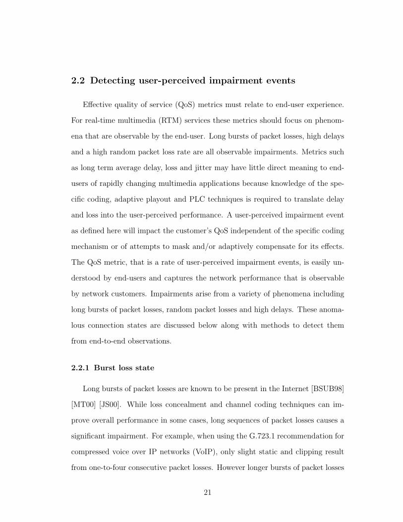
Figure 2.1. Estimated one-way delays and minimum playoutdelay (planetlab2. ashburn.equinix.planet-lab.org and planet-lab1.comet.columbia.edu in Feb, 2004)

Let the one-way delay estimate for RTTi be OWDi and let jWindow be the

window size (e.g. 160 samples). Then, MOi is the sample mean of all one-way

delay samples in a window of jWindow samples and SOi is the sample standard

deviation, i.e.,

MOi = mean{OWDi−jWindow+1, OWDi−jWindow+2, ..., OWDi}

26

SOi = standard deviation{OWDi−jWindow+1, OWDi−jWindow+2, ..., OWDi}

Then, MOi + SOi is one possible estimate of the minimum playout delay that

is needed to avoid excessive packet losses due to late arrivals. Most playout

schemes will likely have a playout delay greater than this minimum. Estimated

one-way delays and minimum playout delays are shown in Figure 2.1. When this

minimum playout delay exceeds a threshold delay (i.e., MOi +SOi > Dmax) then it

is inferred that interactivity for RTM applications is impacted (regardless of the

type of playout scheme really in use) and the connection is defined to be in delay

impairment state. To evaluate this approach, three different thresholds for our

measurements: 100 ms, 150 ms and 200 ms are evaluated.

2.3 Detecting congestion and route changes

Methods for detecting congestion and route changes from end-to-end observa-

tions are presented in this section. The two methods for detecting congestion use

RTT and loss information to infer congestion. Only method 1 is used for detect-

ing congestion events from end-to-end measurements collected over Planet-Lab

nodes. A new method for detecting route changes using only RTT information is

also presented and evaluated using measurements.

2.3.1 Congested state

Congestion is a state of sustained network overload, where demand for re-

sources exceeds the supply for an extended period of time. A congestion event

may cause a number of consecutive packet losses. Congestion may also cause the

random packet loss rate, mean delay and variation of delay to increase signifi-

27

cantly, thus resulting in impairment events. When one or more queues in the

end-to-end connection are congested, the connection is in a congested state. This

section presents two methods for detecting congestion events.

2.3.1.1 Method 1

It is well known that as the load increases, the mean and the variance of waiting

times in queue increase. Specifically, for an M/M/1 queuing system [Kle75], the

mean and the variance of waiting times in queue are given by:

MW =ρ

µ− λσ2W =

ρ(2− ρ)

(µ− λ)2

where λ is the arrival rate, µ service rate and ρ = λµ

is the load.

Let the ratio η = σWMW

(η is the coefficient of variation). Simplifying for η, it follows

that

η =

√2− ρρ

Solving for ρ, there is the equality

ρ =2

η2 + 1(2.1)

Thus, given a set of waiting time samples from an M/M/1 queue, ρ can be es-

timated using the above equation. Clearly, real-world router queues are not ac-

curately modeled as M/M/1 queues. Moreover, waiting time samples from each

individual queue along an end-to-end connection are not observable at the end

nodes. However, equation (2.1) suggests a decision variable that should be corre-

lated to the congestion along an end-to-end path. The pseudo waiting times are

extracted from the RTT samples and used to estimate the value of the decision

28

variable ρ̃.

Let RTTi be the ith RTT sample in ms, then the pseudo waiting time wi is

given by:

wi = RTTi −MinRTT

where MinRTT is the minimum of all RTT samples collected on the current

route. Thus, if j and k are sequence numbers where route change events nearest

to sequence number i occurred (route change detection is discussed later) and

j < i < k, then

MinRTT = min{RTTj, RTTj+1, ..., RTTi−1, RTTi, RTTi+1, ..., RTTk}

However, the minimum RTT of the current route computed using the above pro-

cedure is not always accurate because of the timing issues on Planet-lab nodes

[pla04]. Apparently, the minimum RTT drops to a very low value momentarily

during network time protocol (NTP) resynchronization events. To remove these

minimum RTT outliers caused by timing mechanisms, all RTT samples are re-

moved that have a value less than a 1 percentile value of RTT samples from the

current route. The minimum RTT is then computed using the remaining RTT

samples.

The mean and the standard deviation of the waiting times are estimated over

a window of cWindow samples.

M̃i = mean{wi, wi−1, ..., wi−cWindow+1}

σ̃i = standard deviation{wi, wi−1, ..., wi−cWindow+1}

29

Then, the decision variable ρ̃i is formed by

ρ̃i =2

η̃i2 + 1

where η̃i =σ̃i

M̃i

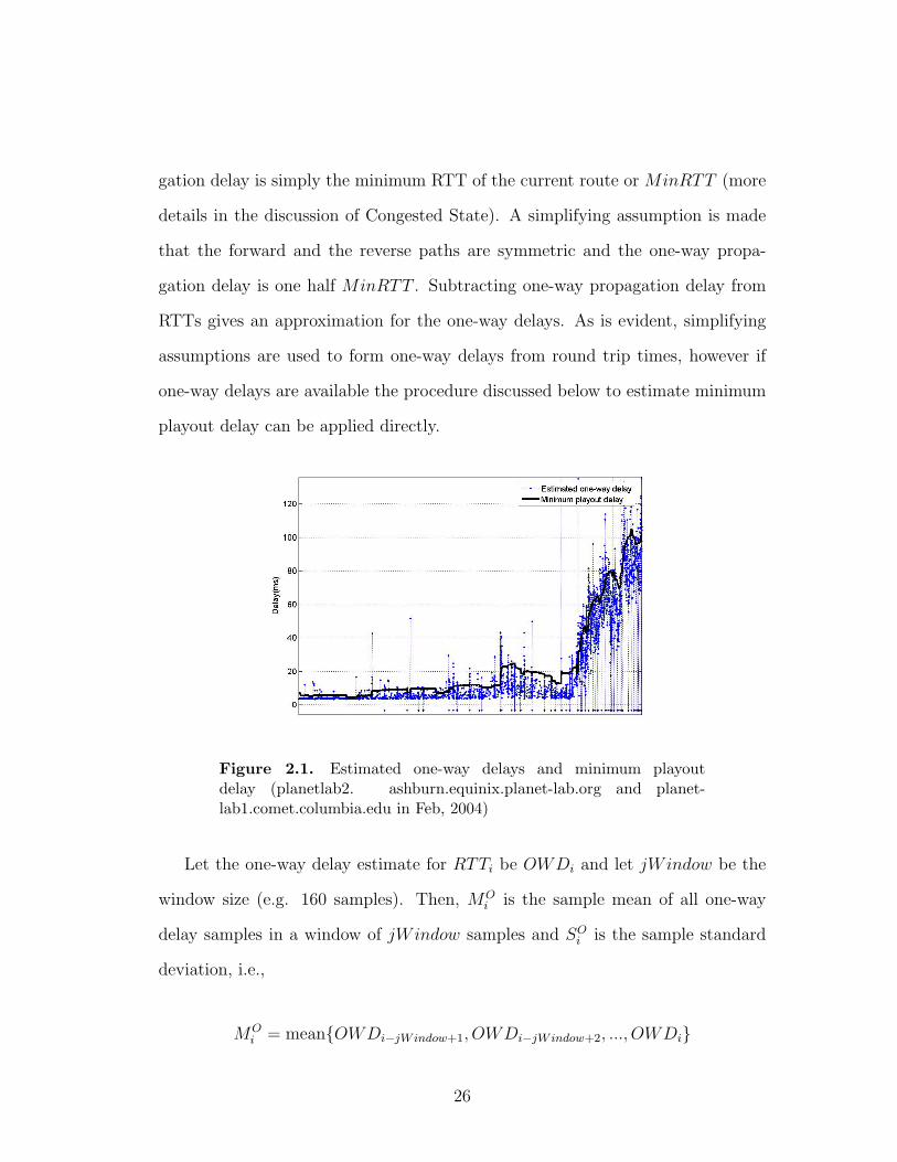
RTTs that are collected over a period of one day are shown along with the

decision variable ρ̃ in Figure 2.2(a). For a period of about 7 to 8 hours during

the day, RTT is much longer than the mean RTT of 15 ms. Variation of RTTs

and packet loss rate also increase substantially during this period. Possibly, one

of the router queues in the end-to-end connection is congested. It is clear from

this figure that the decision variable ρ̃ is correlated with congestion as ρ̃ is higher

during the congestion event.

At first, it might seem that choosing a constant threshold ρT and checking for

the condition ρ̃i > ρT is sufficient to detect congestion. But this method results in

many false positives as ρ̃ is high not only during congestion but also when queues

in the end-to-end path are very lightly loaded. This is illustrated in Figure 2.2(b)

where RTTs are almost the same. Mean and standard deviation of waiting times

are close to zero. However, the decision variable ρ̃ has a value close to 1 for a

significant portion of the trace. This happens because when the queues in the end-

to-end path are very lightly loaded, waiting times w are close to 0. In that case,

the variation in delay is small (e.g. from processing delays in routers, Ethernet

contention delays, etc.). Thus, often σ̃ is less than M̃ , i.e., the ratio η̃ is less than

1 and as a result ρ̃ is greater than 1.

Therefore, to remove the false positives two more conditions are checked. First,

false positives occur when the mean waiting time is small. Thus, if M̃i < MT (e.g.

MT = 5 ms) then the event is a false positive. Second, during congestion when

arrival rate exceeds service rate for an extended period of time, packet losses are

30

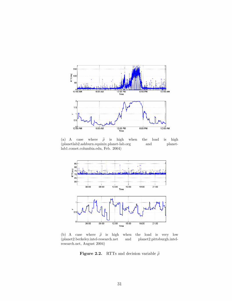
(a) A case where ρ̃ is high when the load is high(planetlab2.ashburn.equinix.planet-lab.org and planet-lab1.comet.columbia.edu, Feb. 2004)

(b) A case where ρ̃ is high when the load is very low(planet2.berkeley.intel-research.net and planet2.pittsburgh.intel-research.net, August 2004)

Figure 2.2. RTTs and decision variable ρ̃

31

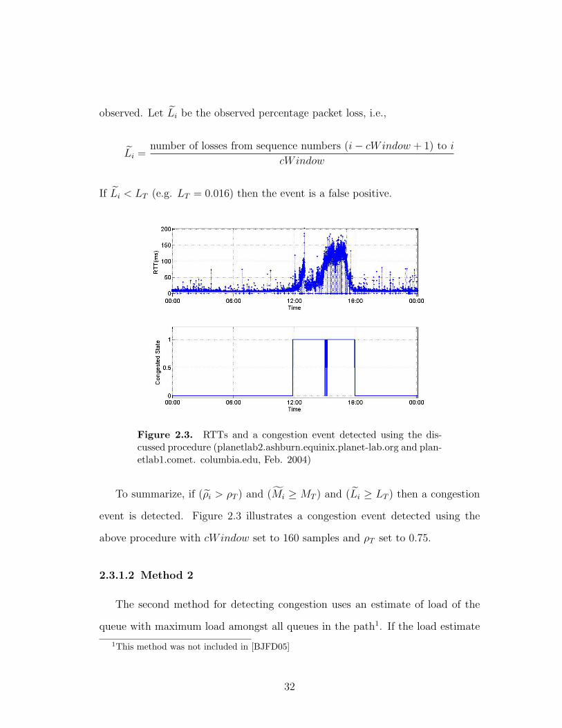
observed. Let L̃i be the observed percentage packet loss, i.e.,

L̃i =number of losses from sequence numbers (i− cWindow + 1) to i

cWindow

If L̃i < LT (e.g. LT = 0.016) then the event is a false positive.

Figure 2.3. RTTs and a congestion event detected using the dis-cussed procedure (planetlab2.ashburn.equinix.planet-lab.org and plan-etlab1.comet. columbia.edu, Feb. 2004)

To summarize, if (ρ̃i > ρT ) and (M̃i ≥ MT ) and (L̃i ≥ LT ) then a congestion

event is detected. Figure 2.3 illustrates a congestion event detected using the

above procedure with cWindow set to 160 samples and ρT set to 0.75.

2.3.1.2 Method 2

The second method for detecting congestion uses an estimate of load of the

queue with maximum load amongst all queues in the path1. If the load estimate

1This method was not included in [BJFD05]

32

is close to 1 and the loss rate is greater than some threshold, then the connection

is in congested state. Load is defined as follows :-

ρ =λ

µ= P (server is busy)

ρ = 1− P (server is idle) (2.2)

Equation 2.2 can be used to form an estimate of the load from end-to-end

measurements as follows. Let MinRTTcW be the minimum of cWindow RTT

samples, i.e.,

MinRTTcW = min{RTTi, RTTi−1, ..., RTTi−cWindow+1}

Also, let MinCount be the number of RTT samples in the window of cWindow

samples, that have a RTT value less than MinRTTcW + ε, where ε is the error

term (e.g., ε = 0.5ms). Then it is conjectured that amongst the cWindow RTT

samples, MinCount samples found the queue empty on arrival2. Then MinCountcWindow

is an estimate of the probability: P (server is idle). From Equation 2.2 load can

be estimated as follows,

ρ̃ = 1− MinCount

cWindow(2.3)

In the above discussion it is assumed that there is only one queue in the path.

However, this method may be used to estimate the load of the queue with max-

imum load in the path under certain conditions3. Note that this load estimation

procedure does not assume any traffic model.

2ε represents the small variable delays like link layer contention delays, processing delays etc.3Future work will include an investigation of these conditions and this could lead to improve-

ments in the load estimation procedure.

33

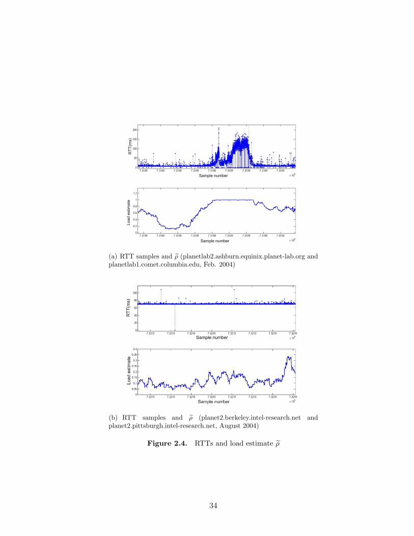
(a) RTT samples and ρ̃ (planetlab2.ashburn.equinix.planet-lab.org andplanetlab1.comet.columbia.edu, Feb. 2004)

(b) RTT samples and ρ̃ (planet2.berkeley.intel-research.net andplanet2.pittsburgh.intel-research.net, August 2004)

Figure 2.4. RTTs and load estimate ρ̃

34

RTTs collected over a period of one day that were shown earlier in Figures

2.2(a) and 2.2(b) are shown again in Figures 2.4(a) and 2.4(b) along with the

load estimate ρ̃. In Figure 2.4(a) mean RTT, variation of RTT and loss rate is

very high for a 7− 8 hour period. It is conjectured that one of the queues in the

end-to-end path is congested. Note that the load estimate ρ̃ is very close to 1

during this entire period of time and is less than 0.95 at all other times. Also, in

Figure 2.4(b) load estimate ρ̃ is less than 0.35 for the entire duration of the trace.

These plots suggest that to detect congestion, it may be sufficient to compare ρ̃

to a load threshold (say ρ[2]T = 0.98). However, if events other than congestion

cause the RTT variation to increase then the load may be overestimated using

this method. To avoid false positives that may be caused by such events, loss

rate can also be compared to a threshold loss rate in addition to comparing the

load estimate to a load threshold. Thus, the connection is in congested state if

(ρ̃ ≥ ρ[2]T ) and (L̃i ≥ LT ).

2.3.2 Route change state

Layer 3 route changes can be detected by comparing routes returned by tracer-

oute. If the route returned by current traceroute is not the same as the route re-

turned by the previous traceroute then the route changed. Route changes can also

be detected by comparing values stored in IP TTL field of arriving probe packets.

If the TTL value of arriving packet is different from the TTL value of a packet that

arrived immediately before the current packet, then it is inferred that there has

been a Layer 3 route change. Since probe packets are sent at a higher rate than

traceroute measurements are performed, route changes are detected faster using

the TTL change method. However, not all route changes cause a TTL change

35

(e.g., when the new route has same number of hops as the old route). Layer 3

route changes may also be detected using the minimum RTT change algorithm

discussed below.

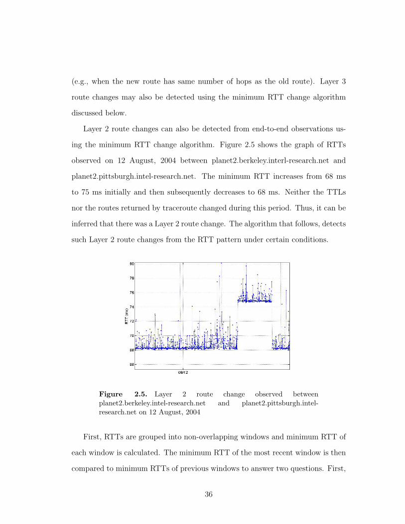
Layer 2 route changes can also be detected from end-to-end observations us-

ing the minimum RTT change algorithm. Figure 2.5 shows the graph of RTTs

observed on 12 August, 2004 between planet2.berkeley.interl-research.net and

planet2.pittsburgh.intel-research.net. The minimum RTT increases from 68 ms

to 75 ms initially and then subsequently decreases to 68 ms. Neither the TTLs

nor the routes returned by traceroute changed during this period. Thus, it can be

inferred that there was a Layer 2 route change. The algorithm that follows, detects

such Layer 2 route changes from the RTT pattern under certain conditions.

Figure 2.5. Layer 2 route change observed betweenplanet2.berkeley.intel-research.net and planet2.pittsburgh.intel-research.net on 12 August, 2004

First, RTTs are grouped into non-overlapping windows and minimum RTT of

each window is calculated. The minimum RTT of the most recent window is then

compared to minimum RTTs of previous windows to answer two questions. First,

36

is the utilization of queues low enough for the Layer 2 route change detection

algorithm to work (see Figure 2.6(a))? If the answer to the first question is yes,

then second, has the minimum RTT changed? A change in the minimum RTT

is either due to a route change or due to random delays possibly arising from

queuing (see Figure 2.6(b)). When the minimum RTT changes, the algorithm

tries to determine whether or not it was caused by a route change.

Minimum RTT is computed as follows. W is the route change window size,

e.g., W = 40 samples. i is the sequence number of the most recent RTT sample.

Si is the set of W sequence numbers, Si = {i, i− 1, i− 2, ..., i−W + 1}. RTT Si

is the set of W RTT samples: RTT Si = {RTTi, RTTi−1, RTTi−2, ..., RTTi−W+1}.

min[RTT Si ] is minimum of all RTTs in the set RTT Si . Then min[RTT Si ] is the

minimum RTT of the current window.

Minimum RTT of the current window is compared to minimum RTTs of the

previous windows. The set prevMinsi stores minimum RTTs of previous win-

dows. numPrevWindowsi is the number of windows since the most recent route

change. If the most recent route change occurred at sequence number j (j < i),

then numPrevWindowsi = b i−j+1Wc. prevMinsi is the set of minimum RTTs of

previous numPrevWindowsi − 1 windows, i.e.,

prevMinsi = {min[RTT Si−W ],min[RTT Si−2W ], ...,min[RTT Si−(numPrevWindows−1)W ]}

The first step in the process is to compare the minimum RTT of the current

window to minimum RTTs of previous windows to determine whether or not vari-

ation in RTTs is low enough for Layer 2 route changes to be detected. Figure

2.6(a) illustrates the case where delay variation is high and Layer 2 route changes

cannot be reliably inferred from the observations. RTTk = FixedDelayk +

V ariableQueuingDelayk + V ariableOtherDelaysk, where FixedDelayk is the

37

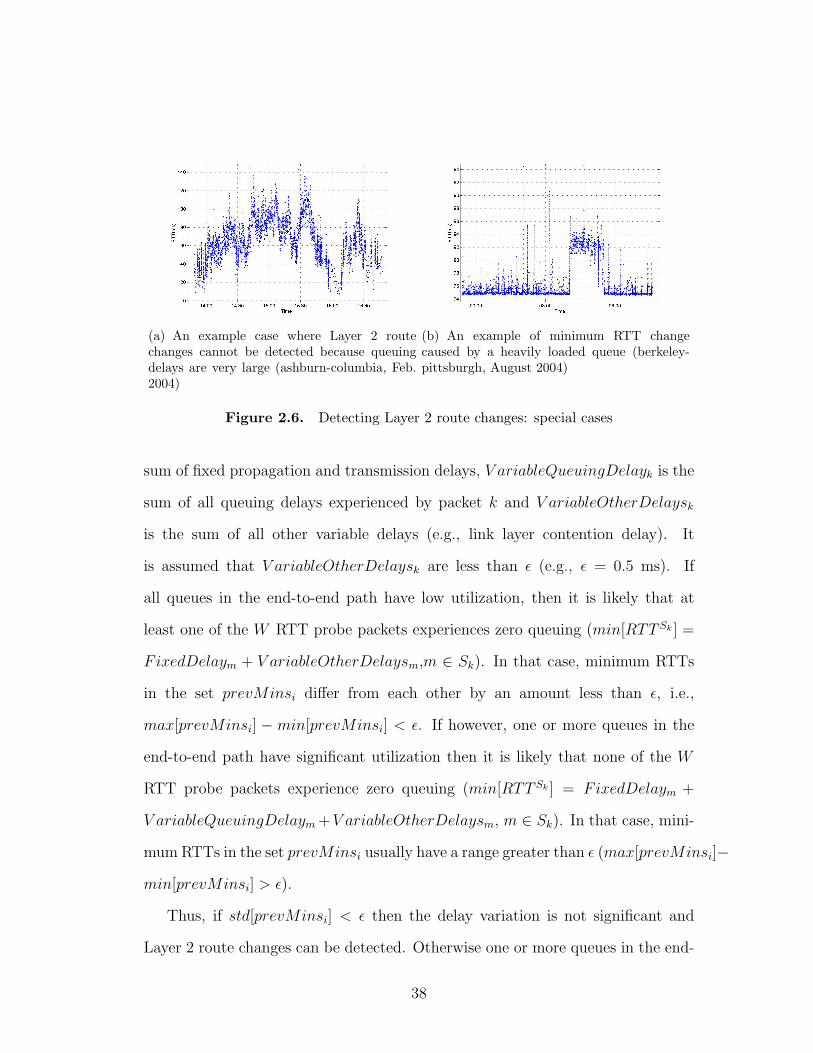
(a) An example case where Layer 2 routechanges cannot be detected because queuingdelays are very large (ashburn-columbia, Feb.2004)

(b) An example of minimum RTT changecaused by a heavily loaded queue (berkeley-pittsburgh, August 2004)

Figure 2.6. Detecting Layer 2 route changes: special cases

sum of fixed propagation and transmission delays, V ariableQueuingDelayk is the

sum of all queuing delays experienced by packet k and V ariableOtherDelaysk

is the sum of all other variable delays (e.g., link layer contention delay). It

is assumed that V ariableOtherDelaysk are less than ε (e.g., ε = 0.5 ms). If

all queues in the end-to-end path have low utilization, then it is likely that at

least one of the W RTT probe packets experiences zero queuing (min[RTT Sk ] =

FixedDelaym + V ariableOtherDelaysm,m ∈ Sk). In that case, minimum RTTs

in the set prevMinsi differ from each other by an amount less than ε, i.e.,

max[prevMinsi] − min[prevMinsi] < ε. If however, one or more queues in the

end-to-end path have significant utilization then it is likely that none of the W

RTT probe packets experience zero queuing (min[RTT Sk ] = FixedDelaym +

V ariableQueuingDelaym +V ariableOtherDelaysm, m ∈ Sk). In that case, mini-

mum RTTs in the set prevMinsi usually have a range greater than ε (max[prevMinsi]−

min[prevMinsi] > ε).

Thus, if std[prevMinsi] < ε then the delay variation is not significant and

Layer 2 route changes can be detected. Otherwise one or more queues in the end-

38

to-end path may be congested and Layer 2 route changes cannot be accurately

detected using this approach.

Next, minimum RTT of current window is compared to minimum RTTs of pre-

vious windows to determine whether or not the minimum RTT has changed. If ei-

thermin[RTT Si ] < (median[prevMinsi]−ε) or ifmin[RTT Si ] > (median[prevMinsi]+

ε) then it is inferred that the minimum RTT has changed.

This minimum RTT change is either caused by a route change or delay vari-

ation possibly caused by queuing in a heavily loaded router queue. Figure 2.6(b)

illustrates minimum RTT change caused by a large delay variation. Minimum

RTT changes from 74 ms to a little over 80 ms in this case. If (median[RTT Si ]−

min[RTT Si ]) < κ (e.g., κ = 1ms) then it is inferred that the minimum RTT

change is caused by a route change. However, it is possible that there is a

Layer 2 route change and one of the switches in the new route is heavily loaded.

To detect that condition, examine γ × W (e.g.γ = 3) more RTT samples. If

(median[RTT Si ]−min[RTT Si ]) > κ ms then γ ×W more RTT samples are col-

lected before it can be decided whether or not it was a route change that caused

the minimum RTT change. Let n = i+ (γ ×W ), where i is the sequence number

of most recent RTT probe packet. Si:n is the set of sequence numbers from i to

n, i.e., Si:n = {i, i+ 1, ..., n− 1, n}. RTT Si:n is the set of RTT samples RTT Si:n =

{RTTi, RTTi+1, ..., RTTn−1, RTTn}. min[RTT Si:n ] is the minimum of all RTTs

in the set RTT Si:n . If for each p, p ∈ Si:n, min[RTT Sp ] ≤ (min[RTT Si:n ] + ε),

then it is inferred that the minimum RTT change is caused by a route change.

Otherwise it is inferred that delay variation caused the minimum RTT change.

If a route change is detected, routes returned by traceroute and TTLs are

compared. If neither traceroutes nor TTLs change, then it is inferred that there

39

Figure 2.7. Layer 2 route change detected using the dis-cussed procedure (planet2. berkeley.intel-research.net andplanet2.pittsburgh.intel-research.net, August 2004)

was a Layer 2 route change. Figure 2.7 illustrates Layer 2 route changes detected

using the above procedure. The RTTs were collected in August 2004 between

planet2.berkeley.intel-research.net and planet2.pittsburgh.intel-research.net. While

the algorithm successfully detected most of the Layer 2 route changes, it failed to

detect the three marked as missed events. Note that when the first missed event

occurred, very few RTT samples (less than (ν + 1) ×W samples) were collected

since the most recent successfully detected route change. The set prevMinsi

should have at least ν (e.g., ν = 3) elements before minimum RTT changes can

be detected. Since, less than W RTT samples were collected in the new route

before another route change occurred, and since the set prevMins was empty,

this route change was not detected. For the second and third missed events, the

minimum RTT changed by 0.4 ms and ε was set to 0.5 ms. Since the algorithm

can detect route changes only when the minimum RTT changes by more than ε

40

ms, these route changes were not detected. In the measurements collected over

the Internet for about 26 days on 9 different node pairs, 96 events were manually

found by visual analysis of RTT data that looked like route changes. The Layer 2

route change algorithm detected 71.8% of these 96 events. The other events were

not detected either because the minimum RTT changed by a value less than ε or

because after the first route change, very few RTT samples were collected in the

new route before the route changed again. The algorithm also generated some

false positives (detected a route change when visually we could not find any route

changes). About 4% of the detected events were false positives.

The minimum RTT of a path can change not only when there is a Layer 2 route

change but also due to a Layer 3 route change. Thus, this algorithm for detecting

Layer 2 route changes can also be used to detect Layer 3 route changes. This is

useful when administrators restrict ICMP response from routers and traceroute

cannot be used to detect Layer 3 route changes. For the measurements that

were conducted, Layer 3 route changes detected using the RTT based algorithm

were compared with the ones detected using traceroute or TTL changes. For

38.7% of all Layer 3 route changes detected using traceroute or TTL changes,

minimum RTT change was not significant (less than ε ms) and hence the RTT

based algorithm did not detect these route changes. About 38.1% of the Layer 3

route changes detected using traceroute or TTL changes were either preceded by

another Layer 3 route change (with less than ν ×W RTT samples between the

two route changes) or followed by another Layer 3 route change (with less than

W RTT samples between the two route changes). These route changes were also

not detected by the RTT based algorithm. We expect the proposed RTT based

algorithm to detect a Layer 3 route change when there are enough RTT samples

41

and the change in RTT is significant; in those cases the technique detected 89.7%

of the route changes. The algorithm missed 10.3% of those Layer 3 route changes.

Future work could lead improvements in the algorithm to increase the probability

of detecting route changes.

2.4 Measurement results

End-to-end measurements were conducted for 26 days on 9 different end-node

pairs connected to the Planet-Lab infrastructure. This section discusses the char-

acteristics of impairment events that were observed in these measurements. Paths

on which congestion events were observed had a large number of high random loss

and burst loss events. Congestion events were observed on two out of the nine

pairs4. Characteristics of these congestion events are discussed. Layer 3 route

changes were observed on all the 9 pairs and Layer 2 route changes on 6 pairs.

Table 2.1 lists the location of end nodes, dates and number of days on which

data was collected. Node pairs for which both end nodes are within the United

States are labeled DC (for Domestic-Commercial) since at least one of the two end

nodes is a non-Internet2 node. When both end nodes are Internet2 nodes (nodes in

a university or a research center), then traffic is routed through Internet2 routers

that have a very low load. For this reason, only pairs were used for which at

least one node is a non-Internet2 node. Node pairs labeled I (International) have

either one or both end nodes outside the United States. There is 21 days of data

for node pairs DC1 and I2, 24 days for DC2 and 26 days for the remaining node

pairs.

Statistics of all detected impairment events are listed in Table 2.2. Rate of

4Method 1 was used to detect congestion

42

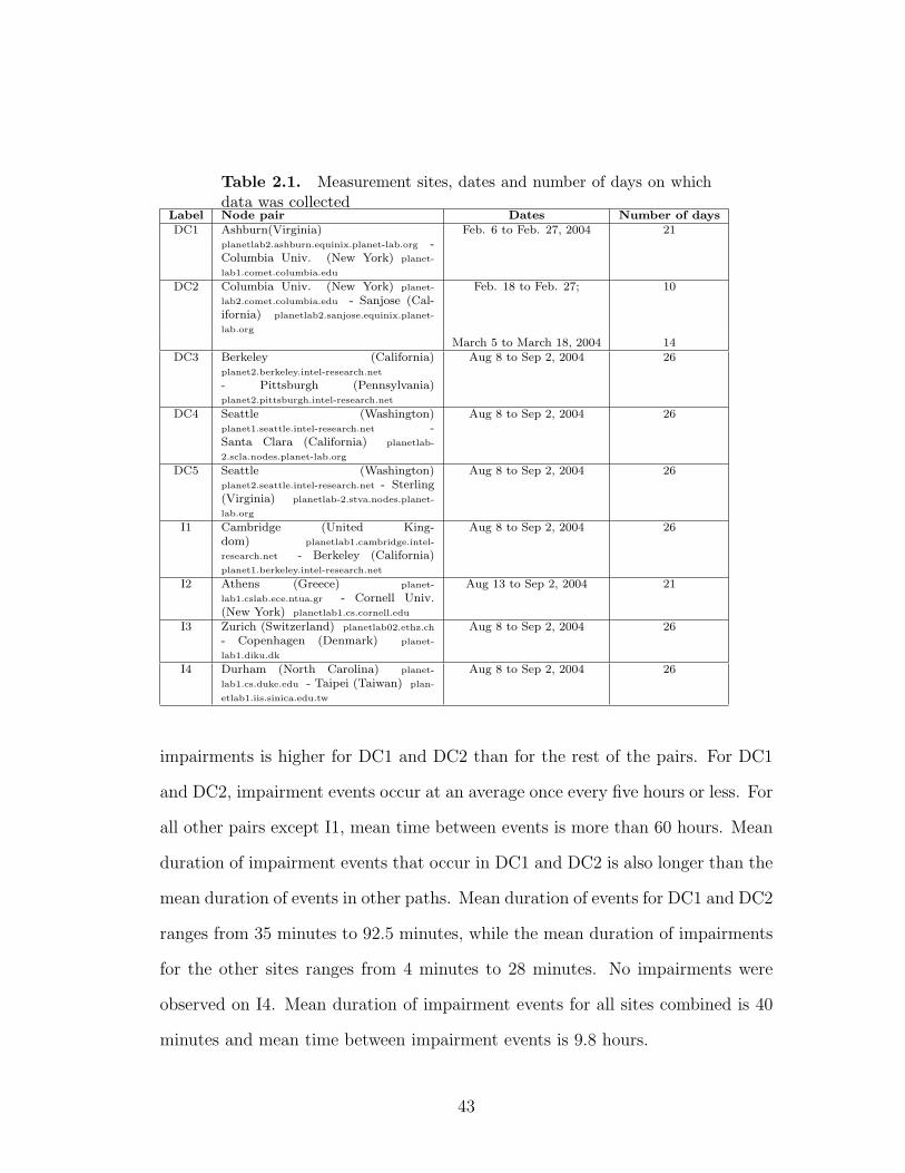
Table 2.1. Measurement sites, dates and number of days on whichdata was collected

Label Node pair Dates Number of daysDC1 Ashburn(Virginia)

planetlab2.ashburn.equinix.planet-lab.org -Columbia Univ. (New York) planet-

lab1.comet.columbia.edu

Feb. 6 to Feb. 27, 2004 21

DC2 Columbia Univ. (New York) planet-

lab2.comet.columbia.edu - Sanjose (Cal-ifornia) planetlab2.sanjose.equinix.planet-

lab.org

Feb. 18 to Feb. 27; 10

March 5 to March 18, 2004 14DC3 Berkeley (California)

planet2.berkeley.intel-research.net

- Pittsburgh (Pennsylvania)planet2.pittsburgh.intel-research.net

Aug 8 to Sep 2, 2004 26

DC4 Seattle (Washington)planet1.seattle.intel-research.net -Santa Clara (California) planetlab-

2.scla.nodes.planet-lab.org

Aug 8 to Sep 2, 2004 26

DC5 Seattle (Washington)planet2.seattle.intel-research.net - Sterling(Virginia) planetlab-2.stva.nodes.planet-

lab.org

Aug 8 to Sep 2, 2004 26

I1 Cambridge (United King-dom) planetlab1.cambridge.intel-

research.net - Berkeley (California)planet1.berkeley.intel-research.net

Aug 8 to Sep 2, 2004 26

I2 Athens (Greece) planet-

lab1.cslab.ece.ntua.gr - Cornell Univ.(New York) planetlab1.cs.cornell.edu

Aug 13 to Sep 2, 2004 21

I3 Zurich (Switzerland) planetlab02.ethz.ch

- Copenhagen (Denmark) planet-

lab1.diku.dk

Aug 8 to Sep 2, 2004 26

I4 Durham (North Carolina) planet-

lab1.cs.duke.edu - Taipei (Taiwan) plan-

etlab1.iis.sinica.edu.tw

Aug 8 to Sep 2, 2004 26

impairments is higher for DC1 and DC2 than for the rest of the pairs. For DC1

and DC2, impairment events occur at an average once every five hours or less. For

all other pairs except I1, mean time between events is more than 60 hours. Mean

duration of impairment events that occur in DC1 and DC2 is also longer than the

mean duration of events in other paths. Mean duration of events for DC1 and DC2

ranges from 35 minutes to 92.5 minutes, while the mean duration of impairments

for the other sites ranges from 4 minutes to 28 minutes. No impairments were

observed on I4. Mean duration of impairment events for all sites combined is 40

minutes and mean time between impairment events is 9.8 hours.

43

Table 2.2. Statistics of user-perceived impairmentsData Set Mean duration of impair-

ments (minutes)Mean time between im-pairments (hours)

Mean number ofimpairments perday

DC1 35.9 3.52 7DC2 (Feb) 92.5 5.22 4

DC2 (March) 37.3 4.95 4.78DC3 9.7 62.97 0.23DC4 4.4 89.44 0.115DC5 15.61 268 0.004

I1 14.5 15.2 1.38I2 28.4 121.17 0.19I3 4.62 122.47 0.15I4 - - 0

Table 2.3 lists the observed mean number of burst loss events, high random loss

events (loss probability > 0.05), congestion events and delay impairment (>100

ms) events per day for each data set. Congestion and high random loss events

occurred only in data sets DC1 and DC2. Mean number of burst loss events per

day in DC1 and DC2 are greater than number of burst loss events in other data

sets.

Table 2.3. Mean number of loss, congestion and delay impairmentevents per day

Data set Mean number ofburst loss eventsper day

Mean numberof high randomloss events (lossrate>5%) perday

Mean numberof congestionevents per day

Mean numberof delay impair-ment (100 ms)events per day

DC1 7 6.7 2.5 2.28DC2 1.125 4.08 1.66 2DC3 0.11 0 0 0.07DC4 0 0 0 0.07DC5 0 0 0 0.07

I1 0.8 0 0 1.57I2 0 0 0 4.76I3 0.07 0 0 3.42I4 0 0 0 0

An interesting trend is observed in both data sets DC1 and DC2. Connection

state alternates between congested and normal states for six to eight hours during

day time on weekdays. This is illustrated using one week of data from DC1 in

Figure 2.8 (day labels on time axes correspond to start of that day). Except for

Sunday night, congestion events started at about 11 AM and lasted until 6 or 7

44

PM on weekdays. On this particular week, congestion events were also observed

on late Sunday night and early Monday morning. Histograms of duration and

time between congestion events for DC1 and DC2 are shown in Figures 2.9(a)

and 2.9(b). Mean duration of congestion is 42.6 minutes and mean time between

congestion events is 4.4 hours.

Figure 2.8. Congestion events observed over a period of one week(DC1)

For DC1 and DC2, burst loss, high random loss and high delay impairments

occurred when the connection was in congested state. For DC1, delay and random

loss impairments occurred for 59.2% of the time while connection was in the

congested state. For DC2, impairments occurred for more than 90% of the time

the connection was in the congested state. Table 2.4 lists the impairment time

during which the connection is not in the congested state. It is clear that most

of the delay and high random loss impairments in DC1 and DC2 occur when the

connection is in the congested state. From a total of 174 burst loss events that

occurred in DC1 and DC2, 61% occurred when the connection was in the congested

45

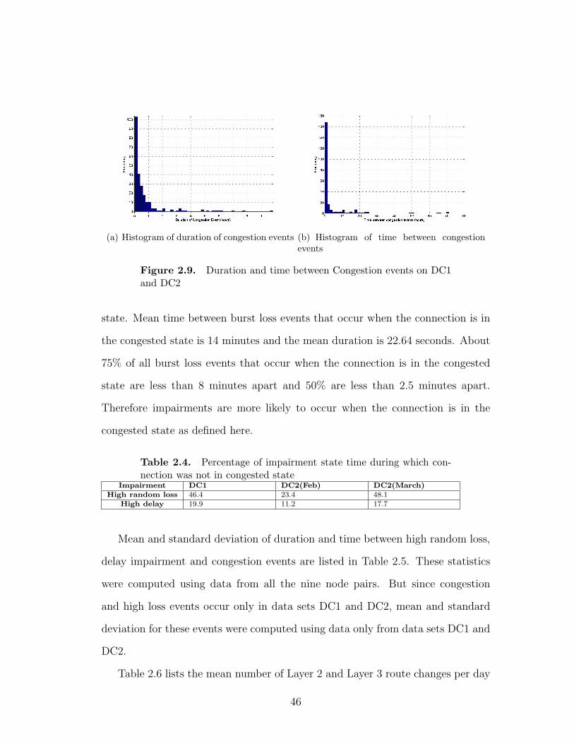
(a) Histogram of duration of congestion events (b) Histogram of time between congestionevents

Figure 2.9. Duration and time between Congestion events on DC1and DC2

state. Mean time between burst loss events that occur when the connection is in

the congested state is 14 minutes and the mean duration is 22.64 seconds. About

75% of all burst loss events that occur when the connection is in the congested

state are less than 8 minutes apart and 50% are less than 2.5 minutes apart.

Therefore impairments are more likely to occur when the connection is in the

congested state as defined here.

Table 2.4. Percentage of impairment state time during which con-nection was not in congested state

Impairment DC1 DC2(Feb) DC2(March)High random loss 46.4 23.4 48.1

High delay 19.9 11.2 17.7

Mean and standard deviation of duration and time between high random loss,

delay impairment and congestion events are listed in Table 2.5. These statistics

were computed using data from all the nine node pairs. But since congestion

and high loss events occur only in data sets DC1 and DC2, mean and standard

deviation for these events were computed using data only from data sets DC1 and

DC2.

Table 2.6 lists the mean number of Layer 2 and Layer 3 route changes per day

46

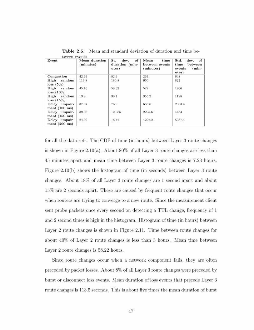
Table 2.5. Mean and standard deviation of duration and time be-tween events

Event Mean duration(minutes)

St. dev. ofduration (min-utes)

Mean timebetween events(minutes)

Std. dev. oftime betweenevents (min-utes)

Congestion 42.63 82.3 264 648High randomloss (5%)

119.8 180.8 666 822

High randomloss (10%)

45.16 58.32 522 1206

High randomloss (15%)

13.9 38.1 355.2 1128

Delay impair-ment (100 ms)

37.07 76.9 685.8 2063.4


39.06 120.85 2295.6 4434


24.99 16.42 4222.2 5987.4

for all the data sets. The CDF of time (in hours) between Layer 3 route changes

is shown in Figure 2.10(a). About 80% of all Layer 3 route changes are less than

45 minutes apart and mean time between Layer 3 route changes is 7.23 hours.

Figure 2.10(b) shows the histogram of time (in seconds) between Layer 3 route

changes. About 18% of all Layer 3 route changes are 1 second apart and about

15% are 2 seconds apart. These are caused by frequent route changes that occur

when routers are trying to converge to a new route. Since the measurement client

sent probe packets once every second on detecting a TTL change, frequency of 1

and 2 second times is high in the histogram. Histogram of time (in hours) between

Layer 2 route changes is shown in Figure 2.11. Time between route changes for

about 40% of Layer 2 route changes is less than 3 hours. Mean time between

Layer 2 route changes is 58.22 hours.

Since route changes occur when a network component fails, they are often

preceded by packet losses. About 8% of all Layer 3 route changes were preceded by

burst or disconnect loss events. Mean duration of loss events that precede Layer 3

route changes is 113.5 seconds. This is about five times the mean duration of burst

47

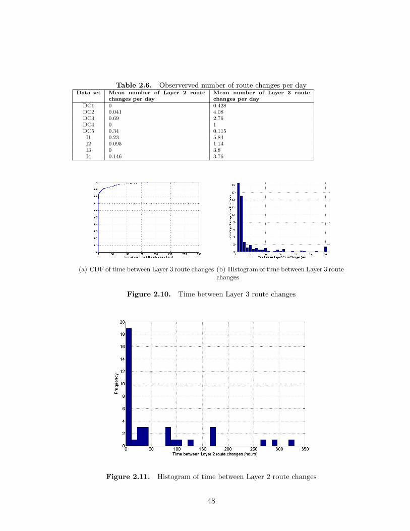
Table 2.6. Observerved number of route changes per dayData set Mean number of Layer 2 route

changes per dayMean number of Layer 3 routechanges per day

DC1 0 0.428DC2 0.041 4.08DC3 0.69 2.76DC4 0 1DC5 0.34 0.115

I1 0.23 5.84I2 0.095 1.14I3 0 3.8I4 0.146 3.76

(a) CDF of time between Layer 3 route changes (b) Histogram of time between Layer 3 routechanges

Figure 2.10. Time between Layer 3 route changes

Figure 2.11. Histogram of time between Layer 2 route changes

48

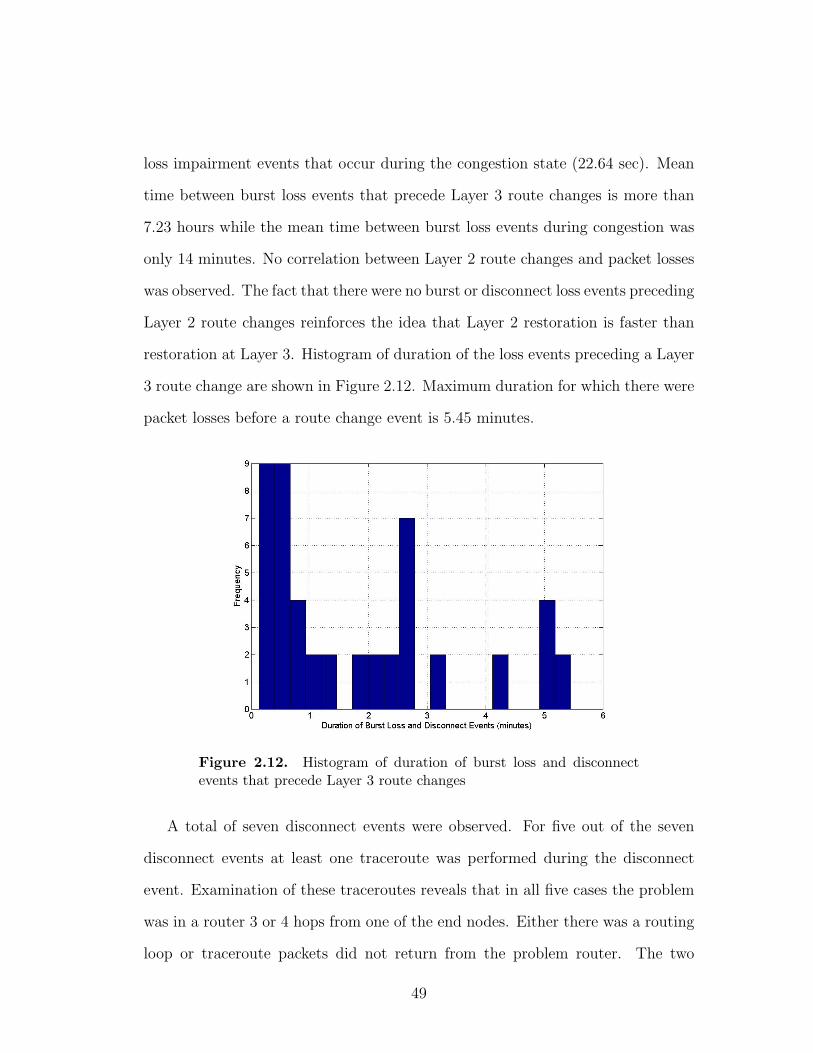
loss impairment events that occur during the congestion state (22.64 sec). Mean

time between burst loss events that precede Layer 3 route changes is more than

7.23 hours while the mean time between burst loss events during congestion was

only 14 minutes. No correlation between Layer 2 route changes and packet losses

was observed. The fact that there were no burst or disconnect loss events preceding

Layer 2 route changes reinforces the idea that Layer 2 restoration is faster than

restoration at Layer 3. Histogram of duration of the loss events preceding a Layer

3 route change are shown in Figure 2.12. Maximum duration for which there were

packet losses before a route change event is 5.45 minutes.

Figure 2.12. Histogram of duration of burst loss and disconnectevents that precede Layer 3 route changes

A total of seven disconnect events were observed. For five out of the seven

disconnect events at least one traceroute was performed during the disconnect

event. Examination of these traceroutes reveals that in all five cases the problem

was in a router 3 or 4 hops from one of the end nodes. Either there was a routing

loop or traceroute packets did not return from the problem router. The two

49

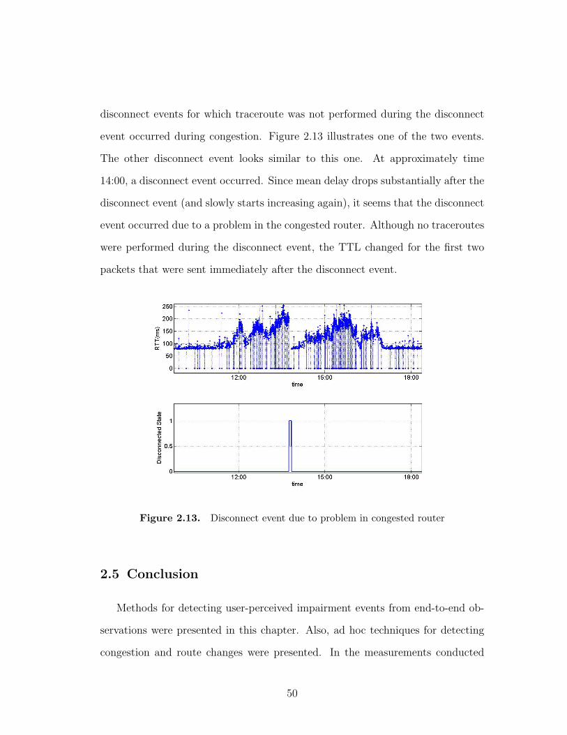
disconnect events for which traceroute was not performed during the disconnect

event occurred during congestion. Figure 2.13 illustrates one of the two events.

The other disconnect event looks similar to this one. At approximately time

14:00, a disconnect event occurred. Since mean delay drops substantially after the

disconnect event (and slowly starts increasing again), it seems that the disconnect

event occurred due to a problem in the congested router. Although no traceroutes

were performed during the disconnect event, the TTL changed for the first two

packets that were sent immediately after the disconnect event.

Figure 2.13. Disconnect event due to problem in congested router

2.5 Conclusion

Methods for detecting user-perceived impairment events from end-to-end ob-

servations were presented in this chapter. Also, ad hoc techniques for detecting

congestion and route changes were presented. In the measurements conducted

50

using the Planet-Lab infrastructure, it was observed that the route change detec-

tion algorithm detected about 71% of all layer 2 route changes. The accuracy of

the ad hoc algorithms discussed in this chapter may be improved by using the

model-based approach. Model-based algorithms for detecting route chages are

presented in the next few chapters. It will be shown in the next few chapters that

the model-based route change detection algorithm has acceptable performance

for a larger region of the parameter space than the heuristics based route change

detection algorithm.

51

Chapter 3

Model-Based Approach: Analysis

3.1 Introduction

A heuristic algorithm for detecting route changes from the RTTs was proposed

and applied to trace data in Chapter 2. Although this algorithm successfully de-

tected a large percentage of the visible route changes, the heuristic nature of this

algorithm precludes the prediction of the expected probabilities of false alarm and

detection. Moreover, this algorithm’s performance cannot be quantifiably tuned.

The probabilities of false alarm and detection measured in Chapter 2 by apply-

ing the detection algorithm on the PlanetLab data are not representative of this

detection algorithm’s performance in general. The heuristic detection algorithm’s

performance depends on the RTTs and the values of its parameters and a user

cannot predict the false alarm and detection probability when this algorithm is

applied on a given data.

This chapter proposes a new model-based algorithm for detecting route changes

whose performance can be predicted. Here RTTs are modeled using a Gamma

distributed random variable (as suggested in [Muk92]). A likelihood ratio pro-

52

vides the foundation for the proposed algorithm. Here, a hypothesis test is used

to determine which of the two alternatives (route change or no route change) is

true when presented with real data. This algorithm for detecting route changes

is named the parameter unaware detector (PUD) because the parameters of the

associated Gamma distributions are not known. PUD estimates these parameters

from the RTT samples and then uses these estimates in the likelihood ratio test to

detect route changes. Closed form expressions that define the PDF of the likeli-

hood ratio under each of the two hypothesis are needed to predict the probabilities

of false alarm and detection. Since PUD uses the estimates of the Gamma distri-

bution parameters in the likelihood ratio test (and not the actual parameters), it

is difficult to derive closed form expressions for PDF of likelihood ratio and thus

predict its performance. Instead of deriving an expression for PDF of likelihood

ratio for PUD, the approach used in this dissertation is to derive expressions for

PDF of likelihood ratio of the parameter aware detector (PAD). Here the values

of the parameters of the associated distribution are assumed to be known. It is

expected that the performance of PUD as a function of the parameters will follows

the same trends as performance of PAD. Also, the PAD is the optimum detector

in the likelihood ratio sense and thus provides the theoretical upper bound for

the performance of any detection algorithm. Any detection algorithm proposed

in the future can be compared to PAD. Deriving the performance of the optimum

detector which provides the performance bound for all algorithms is one of the

contributions of this research. PUD is discussed in section 3.2 followed by PAD in

section 3.3. Expressions for the first two moments of the likelihood ratio for PAD

are also obtained in this chapter in sections 3.4 and 3.5. Chapter 4 illustrates how

these expressions for the first two moments of the likelihood ratio combined with

53

a distribution assumption can be used to predict the probabilities of detection

and false alarms.

3.2 Parameter unaware detector

Round trip time (t) can be modeled by the Gamma distributed random variable

[Muk92] that has the following PDF,

fT (t|α, β, γ) =

1

Γ(α)βα(t− γ)(α−1)e−

(t−γ)β if γ ≤ t <∞

0 otherwise(3.1)

Given n samples (t1, t2, ..., tn), the problem is to determine whether or not there

was a route change when these n samples were collected. Let the composite1

null hypothesis H0 be that all n samples are drawn from Gamma distributed

random variable with parameters α0, β0 and γ0. Also, let the alternative composite

hypothesis H1 be that the first bn2c samples are drawn from a Gamma distributed

random variable with parameters α1, β1 and γ1, and the last dn2e samples are

drawn from a Gamma distributed random variable with parameters α2, β2 and

γ2. Since the parameters α0, β0, γ0, α1, β1, γ1, α2, β2 and γ2 are not known, they

have to be estimated first before the likelihood ratio test can be used. Parameter

γ̂0 is simply the minimum of n samples. Parameters α̂0 and β̂0 are estimated

from all n samples by using the iterative maximum likelihood estimation method

( [MEP93], [Law82], [ME98]). Similarly, α̂1, β̂1, γ̂1 are the estimates formed using

first bn2c samples and α̂2, β̂2, γ̂2 are the estimates formed using last n−bn

2c samples.

1The hypothesis is composite because values of the parameters are not known.

54

Likelihood ratio L is then defined as follows

L = Log

∏ni=1fT (t = ti|α̂0, β̂0, γ̂0)∏bn

2c

i=1fT (t = ti|α̂1, β̂1, γ̂1)∏n

i=bn2c+1fT (t = ti|α̂2, β̂2, γ̂2)

(3.2)

where fT (t = ti|α̂0, β̂0, γ̂0) represents the value obtained by evaluating the function

in Equation 3.1 at ti. Since ti ≥ γ̂0,∀i ∈ {1..n}; ti ≥ γ̂1,∀i ∈ {1..bn2 c} and

ti ≥ γ̂2,∀i ∈ {bn2 c+ 1..n}, Equation 3.2 can be rewritten as follows: -

L = Log

(1

[Γ(α̂0)]nβ̂0nα̂0

∏ni=1(ti − γ̂0)(α̂0−1)e

− (ti−γ̂0)

β̂0

)(

1

[Γ(α̂1)]bn2 cβ̂1

bn2 cα̂1

∏bn2c

i=1(ti − γ̂1)(α̂1−1)e− (ti−γ̂1)

β̂1

)×(

1

[Γ(α̂2)]dn2 eβ̂2

dn2 eα̂2

∏ni=bn

2c+1(ti − γ̂2)(α̂2−1)e

− (ti−γ̂2)

β̂2

)(3.3)

If the likelihood ratio is greater than some threshold λ then the decision is

in favor of H0, otherwise the decision is in favor of H1. The model-based detec-

tion algorithm discussed above was implemented to determine its utility. RTT

samples were generated from a Gamma distributed random variable with pa-

rameters: α = 0.12, β = 1.99. These parameters were estimated from Internet

RTT measurements between planck227.test.ibbt.be (Ghent University, Belgium)

and planetlab1.larc.usp.br (University of Sao Paulo, Brazil) on October 21, 2006.

Minimum RTT is a uniformly distributed random variable between 0 and 10 ms

and this minimum RTT was changed once every 200 samples. The detection algo-

rithm discussed above was applied to this data with its window size (n) fixed at 30

samples. Figure 3.1 illustrates that there is a sharp decrease in the likelihood ratio

whenever there is a route change. There is a significant change in the likelihood

ratio even when the RTT changes by less than 1 ms. All of the route changes in

55

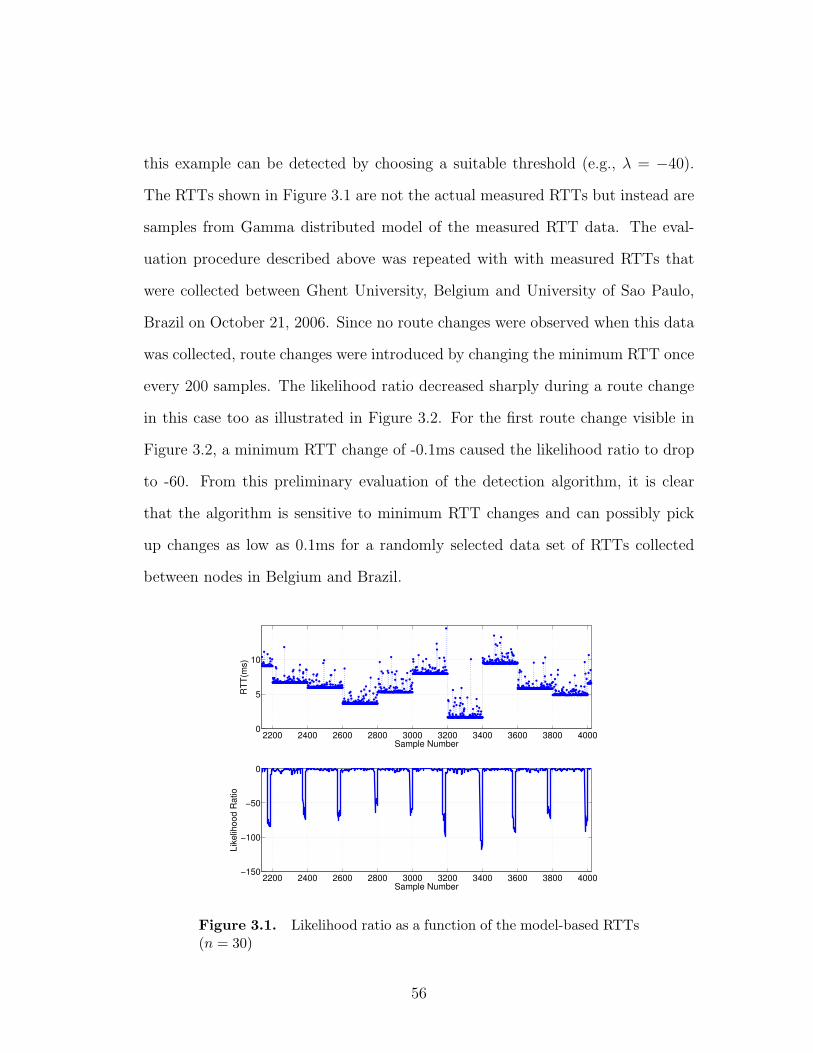
this example can be detected by choosing a suitable threshold (e.g., λ = −40).

The RTTs shown in Figure 3.1 are not the actual measured RTTs but instead are

samples from Gamma distributed model of the measured RTT data. The eval-

uation procedure described above was repeated with with measured RTTs that

were collected between Ghent University, Belgium and University of Sao Paulo,

Brazil on October 21, 2006. Since no route changes were observed when this data

was collected, route changes were introduced by changing the minimum RTT once

every 200 samples. The likelihood ratio decreased sharply during a route change

in this case too as illustrated in Figure 3.2. For the first route change visible in

Figure 3.2, a minimum RTT change of -0.1ms caused the likelihood ratio to drop

to -60. From this preliminary evaluation of the detection algorithm, it is clear

that the algorithm is sensitive to minimum RTT changes and can possibly pick

up changes as low as 0.1ms for a randomly selected data set of RTTs collected

between nodes in Belgium and Brazil.

2200 2400 2600 2800 3000 3200 3400 3600 3800 40000

5

10

Sample Number

RTT(

ms)

2200 2400 2600 2800 3000 3200 3400 3600 3800 4000−150

−100

−50

0

Sample Number

Like

lihoo

d Ra

tio

Figure 3.1. Likelihood ratio as a function of the model-based RTTs(n = 30)

56

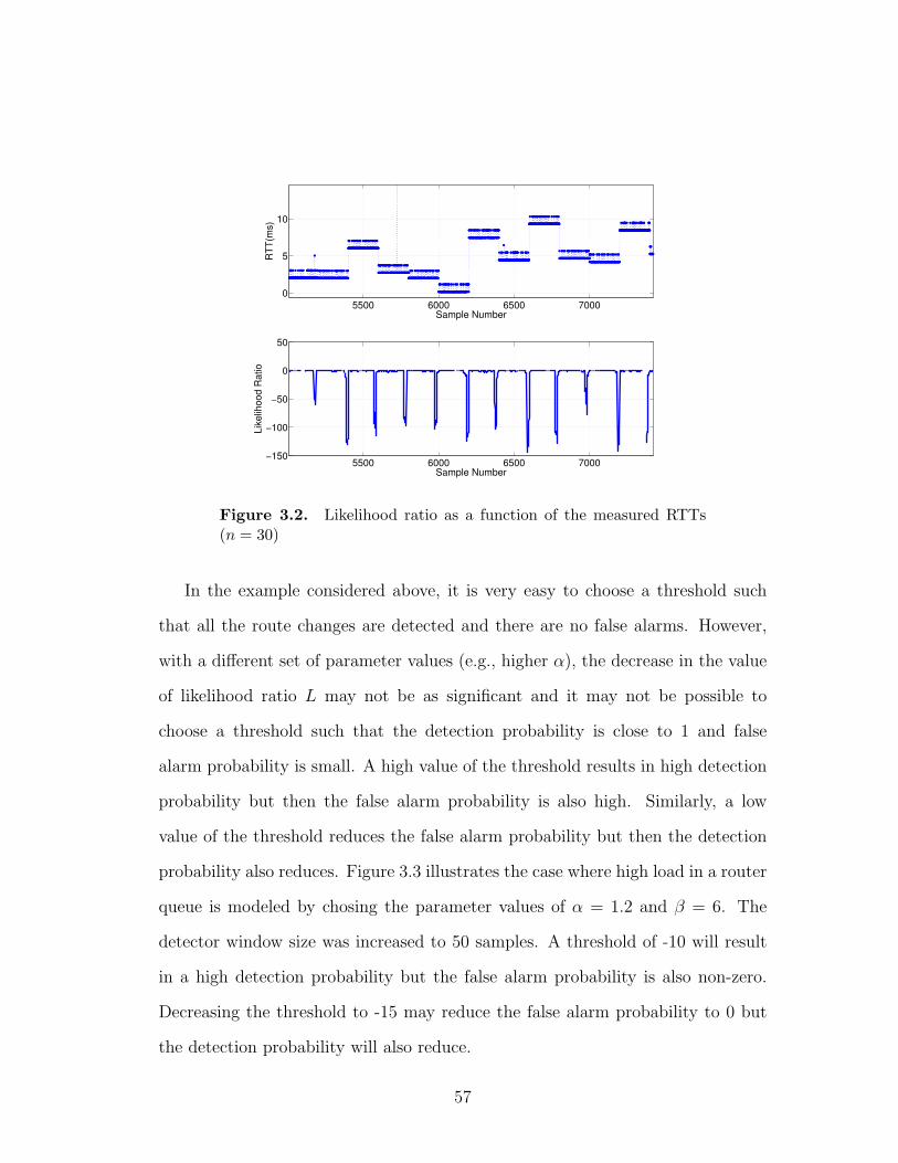
5500 6000 6500 70000

5

10

Sample Number

RTT(

ms)

5500 6000 6500 7000−150

−100

−50

0

50

Sample Number

Like

lihoo

d Ra

tio

Figure 3.2. Likelihood ratio as a function of the measured RTTs(n = 30)

In the example considered above, it is very easy to choose a threshold such

that all the route changes are detected and there are no false alarms. However,

with a different set of parameter values (e.g., higher α), the decrease in the value

of likelihood ratio L may not be as significant and it may not be possible to

choose a threshold such that the detection probability is close to 1 and false

alarm probability is small. A high value of the threshold results in high detection

probability but then the false alarm probability is also high. Similarly, a low

value of the threshold reduces the false alarm probability but then the detection

probability also reduces. Figure 3.3 illustrates the case where high load in a router

queue is modeled by chosing the parameter values of α = 1.2 and β = 6. The

detector window size was increased to 50 samples. A threshold of -10 will result

in a high detection probability but the false alarm probability is also non-zero.

Decreasing the threshold to -15 may reduce the false alarm probability to 0 but

the detection probability will also reduce.

57

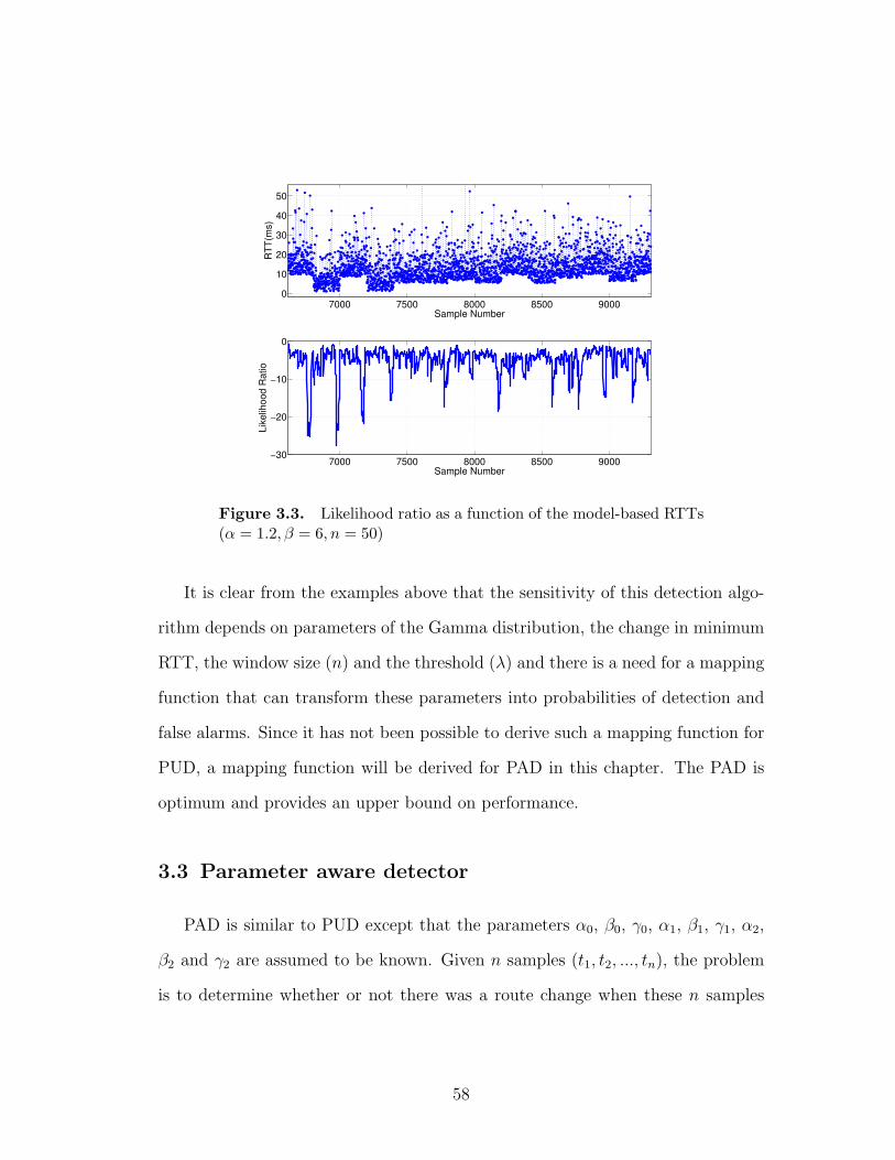
7000 7500 8000 8500 90000

10

20

30

40

50

Sample Number

RTT(

ms)

7000 7500 8000 8500 9000−30

−20

−10

0

Sample Number

Like

lihoo

d Ra

tio

Figure 3.3. Likelihood ratio as a function of the model-based RTTs(α = 1.2, β = 6, n = 50)

It is clear from the examples above that the sensitivity of this detection algo-

rithm depends on parameters of the Gamma distribution, the change in minimum

RTT, the window size (n) and the threshold (λ) and there is a need for a mapping

function that can transform these parameters into probabilities of detection and

false alarms. Since it has not been possible to derive such a mapping function for

PUD, a mapping function will be derived for PAD in this chapter. The PAD is

optimum and provides an upper bound on performance.

3.3 Parameter aware detector

PAD is similar to PUD except that the parameters α0, β0, γ0, α1, β1, γ1, α2,

β2 and γ2 are assumed to be known. Given n samples (t1, t2, ..., tn), the problem

is to determine whether or not there was a route change when these n samples

58

were collected. The simple2 null hypothesis H0 is that all n samples are drawn

from Gamma distributed random variable with parameters α0, β0 and γ0. The

alternative simple hypothesis H1 is that the first bn2c samples are drawn from

a Gamma distributed random variable with parameters α1, β1 and γ1, and the

last dn2e samples are drawn from a Gamma distributed random variable with

parameters α2, β2 and γ2. Since it is assumed that the parameters α0, β0, γ0, α1,

β1, γ1, α2, β2 and γ2 are known, there is no need to estimate these parameters.

The likelihood ratio can then be evaluated using the following equation.

L = Log

∏ni=1fT (t = ti|α0, β0, γ0)∏bn

2c

i=1fT (t = ti|α1, β1, γ1)∏n

i=bn2c+1fT (t = ti|α2, β2, γ2)

(3.4)

If the value of L obtained from Equation 3.4 above is greater than threshold λ then

hypothesis H0 (no route change) is true, otherwise hypothesis H1 (rotue change)

is true. PAD is an ideal detector because it is assumed that the values of the

parameters are known and with this knowledge, PAD has the best performance

amongst all possible detectors in the likelihood ratio sense.

If the PDF of L when H0 is true and the PDF of L when H1 is true are

known then the probability of false alarms and detection can be predicted for a

given value of the threshold. The first two moments of L as a function of the 10

parameters α0, β0, γ0, α1, β1, γ1, α2, β2, γ2 and n are derived in sections 3.4 and

3.5 for hypothesis H0 and H1 respectively. To determine an appropriate threshold

and associated probabilities of detection and false alarms, it is assumed that the

conditional PDFs are Gaussian. This assumption is validated using simulation.

2The hypothesis is simple because the values of the parameters are known.

59

3.4 Moments of L: H0 true

In this section, expressions for the first two moments of L when H0 is true

are derived. It is very difficult to derive an expression for PDF of L and for this

reason only the first two moments are derived and then a Gaussian distribution

is assumed. The base parameter space can be partitioned into two subspaces and

the moments of L are found using different methods for each of the two subspaces.

The two parameter subspaces are named L-finite subspace and L-infinite subspace

and section 3.4.1 discusses why the parameter space is partitioned. Expressions for

expected value of L and variance of L when parameters are in the L-finite subspace

are derived in Sections 3.4.2 and 3.4.3 respectively. Expressions for expected value

of L and variance of L when parameters are in the L-infinite subspace are derived

in Sections 3.4.4 and 3.4.5 respectively.

3.4.1 Parameter subspaces

When parameter values are such that γ0 ≥ Max(γ1, γ2), the parameters are

in the L-finite subspace because L is always finite in this subspace. However,

when parameter values are such that γ0 < Max(γ1, γ2), the parameters are in the

L-infinite subspace because L may be either finite or infinite. When parameters

are in the L-infinite subspace the probability that L is infinite is nonzero. Since

it is assumed that hypothesis H0 is true, all of the n samples are from a Gamma

distribution with parameters α0, β0 and γ0. When γ0 < Max(γ1, γ2), one of the

following is true: (γ0 < γ1,γ0 ≥ γ2) or (γ0 ≥ γ1,γ0 < γ2) or (γ0 < γ1,γ0 < γ2).

When ti < γ1, i ∈ {1..bn2 c} or ti < γ2, i ∈ {bn2 c+ 1..n} for one or more samples ti,

then L =∞ (See Equations 3.1 and 3.4). When L =∞, there is no ambiguity in

deciding in favor of H0 because P (L =∞|H1) = 0. The probability that L is finite

60

when parameters are in the L-infinite subspace will be derived in this section. This

probability will be useful later when expressions for probability of false alarms and

detection are derived. When parameters are in L-infinite subspace, then one of

the following is true: -

• γ2 > γ0 ≥ γ1

• γ1 > γ0 ≥ γ2

• γ2 > γ0 and γ1 > γ0

Expressions for the probability that L is finite (or infinite) will be obtained for

each of the three cases. Probability that ti > ξ,∀i : i ∈ {1..n} (ξ is a constant,

ξ ≥ γ0) can be evaluated as follows

P (ti > ξ, ∀i : i ∈ {1..n}) = P (Min[ti, i ∈ {1..n}] > ξ) (3.5)

The probability P (Min[ti, i ∈ {1..n}] > ξ) can be computed using order statistics.

PDF of the kth order statistic is as follows (from [HC95])

gk(yk) =

n!

(k−1)!(n−k)![F (yk)]

(k−1) [1− F (yk)](n−k) f(yk) 0 ≤ yk <∞

0 otherwise

Here F (y) is the CDF and f(y) is the PDF of the random variable from which

samples are drawn. For a two parameter (γ = 0) Gamma distributed random

variable, PDF of the first order statistic is as follows

g1(y1) =

ny

(α−1)1 e

− y1β

[Γ(α)]nβα

[Γ(α, y1

β

)]n−1

0 ≤ y <∞

0 otherwise

61

The probability P (Min[ti, i ∈ {1..n}] > ξ) is then the integration of this PDF

(g1(y1)) for y1 ranging from ξ − γ0 to ∞.

P (Min[ti, i ∈ {1..n}] > ξ) =n

[Γ(α)]nβα

∫ ∞ξ−γ0

qα0−1e− qβ0

[Γ(α0,

q

β0

)

]n−1

dq (3.6)

Form Equation 3.5, it follows that

P (ti > ξ,∀i : i ∈ {1..n}) = n[Γ(α0)]nβ

α00

∫∞ξ−γ0

qα0−1e− qβ0

[Γ(α0,

qβ0

)]n−1

dq (3.7)

The expressions for the probability that L is finite for each of the three cases can

be derived from Equation 3.7 as follows.

• γ2 > γ0 ≥ γ1

P (L 6=∞) = PLF |H0 = P (ti > γ2,∀i : i ∈ {bn2c+ 1..n})

=dn

2e

[Γ(α0)]dn2 eβ

α00

∫∞γ2−γ0

qα0−1e− qβ0

[Γ(α0,

qβ0

)]dn

2e−1

dq(3.8)

• γ1 > γ0 ≥ γ2

P (L 6=∞) = PLF |H0 = P (ti > γ1,∀i : i ∈ {1..bn2c})

=bn

2c

[Γ(α0)]bn2 cβ

α00

∫∞γ1−γ0

qα0−1e− qβ0

[Γ(α0,

qβ0

)]bn

2c−1

dq(3.9)

62

• γ2 > γ0 and γ1 > γ0

P (L 6=∞) = PLF |H0

= P ([ti > γ2,∀i : i ∈ {bn2c+ 1..n}] and [ti > γ1,∀i : i ∈ {1..bn

2c}])

=

(dn

2e

[Γ(α0)]dn2 eβ

α00

∫∞γ2−γ0

qα0−1e− qβ0

[Γ(α0,

qβ0

)]dn

2e−1

dq

)×(

bn2c

[Γ(α0)]bn2 cβ

α00

∫∞γ1−γ0

qα0−1e− qβ0

[Γ(α0,

qβ0

)]bn

2c−1

dq

)(3.10)

Equations 3.8, 3.9 and 3.10 can be used to predict the probability that L is finite

given that H0 is true and parameters are in L-infinite subspace. These will be

used later in Chapter 4 when receiver operating characteristics are discussed. An

expression for expected value of L when parameters are in the L-finite subspace

will be obtained next in section 3.4.2.

3.4.2 Expected value: L-finite

When the parameters are in the L-finite subspace (i.e., γ0 ≥ Max(γ1, γ2)),

likelihood ratio L is always finite and can be expressed as follows (from Equations

3.4 and 3.1).

L = Log

1[Γ(α0)β0

α0 ]n

∏ni=1 (ti − γ0)(α0−1)e

− (ti−γ0)

β0(1

[Γ(α1)β1α1 ]b

n2 c

∏bn2c

i=1 (ti − γ1)(α1−1)e− (ti−γ1)

β1

)×(

1

[Γ(α2)β2α2 ]d

n2 e

∏ni=bn

2c+1 (ti − γ2)(α2−1)e

− (ti−γ2)

β2

)

63

This equation can be rewritten as follows

L = −nLog[Γ(α0)]− nα0Log[β0] +∑n

i=1(α0 − 1)Log(ti − γ0)−∑n

i=1(ti−γ0)β0

+bn2cLog[Γ(α1)] + bn

2cα1Log[β1]−

∑bn2c

i=1(α1 − 1)Log(ti − γ1)

+∑bn

2c

i=1(ti−γ1)β1

+ dn2eLog[Γ(α2)] + dn

2eα2Log[β2]

−∑n

i=bn2c+1(α2 − 1)Log(ti − γ2) +

∑ni=bn

2c+1

(ti−γ2)β2

(3.11)

Expected value E[L|H0] can then be expressed as follows

E[L|H0] = −nLog[Γ(α0)]− nα0Log[β0] +∑n

i=1(α0 − 1)E[Log(ti − γ0)]

−∑n

i=1(E[ti]−γ0)

β0+ bn

2cLog[Γ(α1)] + bn

2cα1Log[β1]

−∑bn

2c

i=1(α1 − 1)E[Log(ti − γ1)] +∑bn

2c

i=1(E[ti]−γ1)

β1+ dn

2eLog[Γ(α2)]

+dn2eα2Log[β2]−

∑ni=bn

2c+1(α2 − 1)E[Log(ti − γ2)]

+∑n

i=bn2c+1

(E[ti]−γ2)β2

(3.12)

Since it is assumed that H0 is true, E[ti] = γ0 + α0β0. Substituting, there is the

equality

E[L|H0] = −nLog[Γ(α0)]− nα0Log[β0] +∑n

i=1(α0 − 1)E[Log(ti − γ0)]− nα0

+bn2cLog[Γ(α1)] + bn

2cα1Log[β1]−

∑bn2c

i=1(α1 − 1)E[Log(ti − γ1)]

+bn2cγ0+α0β0−γ1

β1+ dn

2eLog[Γ(α2)] + dn

2eα2Log[β2]

−∑n

i=bn2c+1(α2 − 1)E[Log(ti − γ2)] + dn

2eγ0+α0β0−γ2

β2

(3.13)

Expressions for E[Log(ti − γ0)], E[Log(ti − γ1)] and E[Log(ti − γ2)] are needed

to solve the above equation further. While there are no known expressions for

E[Log(ti−γ1)] and E[Log(ti−γ2)], the term E[Log(ti−γ0)] can be solved further

as follows. Let T is a Gamma distributed random variable with parameters α0,

64

β0 and γ0 (RTTs). Also, let Y be a random variable such that Y = T − γ0.

Random variable Y is then a 2 parameter Gamma distributed random variable

with parameters α0 and β0. Expected value E[logY ] then is same as the expected

value E[Log(ti − γ0)]. The moment generating function of Y can be obtained as

follows.

M(u) = E(euLog(y)) = 1Γ(α0)β

α00

∫∞0euLog(y)y(α0−1)e

(− yβ0

)dy

= 1Γ(α0)β

α00

∫∞0yuy(α0−1)e

(− yβ0

)dy

=βu0 Γ(u+α0)

Γ(α0)

The cumulant generating function is then

K(u) = Log[M(u)] = uLog(β0) + Log[Γ(u+ α0)]− Log[Γ(α0)]

Hence, the first cumulant is

κ1(LogY ) = Log(β0) + dduLog[Γ(u+ α0)]

∣∣u=0

= Log(β0) + ddα0Log[Γ(α0)]

= Log(β0) + ψ(α0)

where ψ denotes the digamma function [NJB94], [BK46]. Therefore,

κ1(LogY ) = E[LogY ] = E[Log(T − γ0)] = Log(β0) + ψ(α0) (3.14)

Although simplified expression for E[Log(T − γ0)] is derived above, to the best of

our knowledge, there is no simple expression for E[Log(T−γi)], i = {1, 2}. For this

reason, numerical integration is used to find the value of E[Log(t−γi)], i = {1, 2}.

The value obtained using numerical integration will be denoted by the function

65

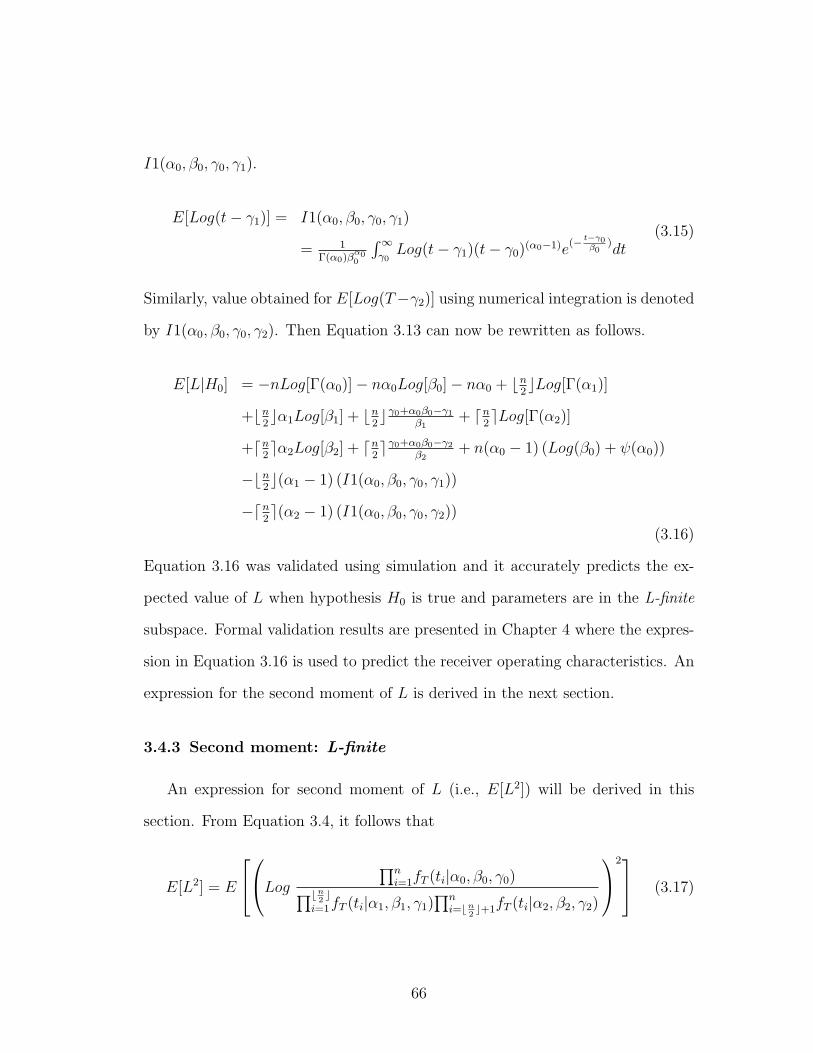
I1(α0, β0, γ0, γ1).

E[Log(t− γ1)] = I1(α0, β0, γ0, γ1)

= 1Γ(α0)β

α00

∫∞γ0Log(t− γ1)(t− γ0)(α0−1)e

(− t−γ0β0

)dt

(3.15)

Similarly, value obtained for E[Log(T−γ2)] using numerical integration is denoted

by I1(α0, β0, γ0, γ2). Then Equation 3.13 can now be rewritten as follows.

E[L|H0] = −nLog[Γ(α0)]− nα0Log[β0]− nα0 + bn2cLog[Γ(α1)]

+bn2cα1Log[β1] + bn

2cγ0+α0β0−γ1

β1+ dn

2eLog[Γ(α2)]

+dn2eα2Log[β2] + dn

2eγ0+α0β0−γ2

β2+ n(α0 − 1) (Log(β0) + ψ(α0))

−bn2c(α1 − 1) (I1(α0, β0, γ0, γ1))

−dn2e(α2 − 1) (I1(α0, β0, γ0, γ2))

(3.16)

Equation 3.16 was validated using simulation and it accurately predicts the ex-

pected value of L when hypothesis H0 is true and parameters are in the L-finite

subspace. Formal validation results are presented in Chapter 4 where the expres-

sion in Equation 3.16 is used to predict the receiver operating characteristics. An

expression for the second moment of L is derived in the next section.

3.4.3 Second moment: L-finite

An expression for second moment of L (i.e., E[L2]) will be derived in this

section. From Equation 3.4, it follows that

E[L2] = E

Log ∏ni=1fT (ti|α0, β0, γ0)∏bn

2c

i=1fT (ti|α1, β1, γ1)∏n

i=bn2c+1fT (ti|α2, β2, γ2)

2 (3.17)

66

Right hand side of the above equation can be expanded as illustrated in the

following steps.

E[L2] = E

∑n

i=1LogfT (ti|α0, β0, γ0)−∑bn

2c

i=1LogfT (ti|α1, β1, γ1)

−∑n

i=bn2c+1LogfT (ti|α2, β2, γ2)

2

E[L2] = E

∑ni=1LogfT (ti|α0, β0, γ0)−

∑bn2c


−∑n


× ∑ni=1LogfT (ti|α0, β0, γ0)−

∑bn2c


−∑n


E[L2] = E

∑ni=1

∑nj=1 (Logf(ti|α0, β0, γ0)× Logf(tj|α0, β0, γ0))

−∑n

i=1

∑bn2c

j=1 (Logf(ti|α0, β0, γ0)× Logf(tj|α1, β1, γ1))

−∑n

i=1

∑nj=bn

2c+1 (Logf(ti|α0, β0, γ0)× Logf(tj|α2, β2, γ2))

−∑n

i=1

∑bn2c


+∑bn

2c

i=1

∑bn2c


+∑bn

2c

i=1

∑nj=bn


−∑n

i=1

∑nj=bn


+∑bn

2c

i=1

∑nj=bn


+∑n

i=bn2c+1

∑nj=bn


(3.18)

67

Solving, there is the equality

E[L2] =

∑ni=1

∑nj=1E [Logf(ti|α0, β0, γ0)× Logf(tj|α0, β0, γ0)]

+∑bn

2c

i=1

∑bn2c

j=1 E [Logf(ti|α1, β1, γ1)× Logf(tj|α1, β1, γ1)]

+∑n

i=bn2c+1

∑nj=bn

2c+1 E [Logf(ti|α2, β2, γ2)× Logf(tj|α2, β2, γ2)]

−2∑n

i=1

∑bn2c

j=1E [Logf(ti|α0, β0, γ0)× Logf(tj|α1, β1, γ1)]

−2∑n

i=1

∑nj=bn

2c+1 E [Logf(ti|α0, β0, γ0)× Logf(tj|α2, β2, γ2)]

+2∑bn

2c

i=1

∑nj=bn

2c+1E [Logf(ti|α1, β1, γ1)× Logf(tj|α2, β2, γ2)]

(3.19)

In the next step, it is assumed that the samples ti and tj are independent iden-

tically distributed. This assumption is valid for RTT measurements considered

here. Also, terms for which i = j have been separated.

E[L2] =

∑ni=1E [Log2f(ti|α0, β0, γ0)]

+∑n

i=1

∑nj=1,j 6=iE [Logf(ti|α0, β0, γ0)]× E [Logf(tj|α0, β0, γ0)]

+∑bn

2c

i=1 E [Log2f(ti|α1, β1, γ1)]

+∑bn

2c

i=1

∑bn2c

j=1,j 6=iE [Logf(ti|α1, β1, γ1)]× E [Logf(tj|α1, β1, γ1)]

+∑n

i=bn2c+1E [Log2f(ti|α2, β2, γ2)]

+∑n

i=bn2c+1

∑nj=bn

2c+1,j 6=iE [Logf(ti|α2, β2, γ2)]× E [Logf(tj|α2, β2, γ2)]

−2∑bn

2c

i=1 E [Logf(ti|α0, β0, γ0)× Logf(ti|α1, β1, γ1)]

−2∑n

i=1

∑bn2c

j=1,j 6=iE [Logf(ti|α0, β0, γ0)]× E [Logf(tj|α1, β1, γ1)]

−2∑n

i=bn2c+1 E [Logf(ti|α0, β0, γ0)× Logf(ti|α2, β2, γ2)]

−2∑n

i=1

∑nj=bn

2c+1,j 6=iE [Logf(ti|α0, β0, γ0)]× E [Logf(tj|α2, β2, γ2)]

+2∑bn

2c

i=1

∑nj=bn

2c+1E [Logf(ti|α1, β1, γ1)]× E [Logf(tj|α2, β2, γ2)]

(3.20)

68

Since it is assumed that ti > Max(γ1, γ2),∀i : i ∈ {1..n}, parts of the right hand

side of Equation 3.20 are expanded below.

E [Log2fT (ti|α0, β0, γ0)] =

Log2Γ(α0) + 2LogΓ(α0)α0Log(β0)

−2(α0 − 1)LogΓ(α0)E [Log(ti − γ0)] + 2LogΓ(α0)E[ti−γ0

β0

]+α2

0Log2(β0)− 2(α0 − 1)α0Log(β0)E [Log(ti − γ0)]

+2α0Log(β0)E[ti−γ0

β0

]+ (α0 − 1)2E [Log2(ti − γ0)]

−2(α0 − 1)E[Log(ti − γ0) ti−γ0

β0

]+ E

[(ti−γ0)2

β20

]

(3.21)

Expressions for expected values needed to solve this equation further are obtained

below. An expression for expected value E[Log(ti − γ0)] that was derived in

Equation 3.14 can be substituted in the right hand side of Equation 3.21 to solve

it further.

E[Log(ti − γ0)] = Log(β0) + ψ(α0)

Also, since T is Gamma distributed with parameters α0, β0 and γ0, E[ti−γ0

β0

]can

be expressed as follows.

E

[ti − γ0

β0

]=γ0 + α0β0 − γ0

β0

= α0

In the derivation of Equation 3.14, the first derivative of the cumulant generating

function was obtained. The second derivative of this same cumulant generating

function can be used to find E[Log2(ti − γ0)]. The cumulant generating function

is as follows.

K(u) = Log[M(u)] = uLog(β0) + Log[Γ(u+ α0)]− Log[Γ(α0)]

69

The second derivative of this function at u = 0 is the variance of the random

variable Log(T − γ0).

σ2 =d2

du2K(u)

∣∣∣∣u=0

= κ2(Log(ti − γ0)) = E[Log2(ti − γ0)]− (E[Log(ti − γ0)])2

The second moment of the random variable Log(T −γ0) can be obtained from the

expected value and variance as follows.

E[Log2(ti − γ0)] =d2

du2K(u)

∣∣∣∣u=0

− (E[Log(ti − γ0)])2

E[Log2(ti − γ0)] = ψ(1)(α0) + (Log(β0) + ψ(α0))2

= ψ(1)(α0) + Log2(β0) + (ψ(α0))2 + 2Log(β0)ψ(α0)

An expression for E[Log(ti − γ0) ti−γ0

β0

]can also be derived from Equation 3.14

as follows. Recall that random variable Y is related to the random variable T by

Y = T − γ0.

1Γ(α0)β

α00

∫∞0Log(y)yα0−1e

− yβ0 dy = Log(β0) + ψ(α0)

1

Γ(α0+1)β(α0+1)0

∫∞0Log(y)y(α0+1)−1e

− yβ0 dy = [Log(β0) + ψ(α0 + 1)]

1

Γ(α0+1)β(α0+1)0

∫∞0Log(y)yyα0−1e

− yβ0 dy = [Log(β0) + ψ(α0 + 1)]

1

Γ(α0+1)β(α0+1)0

∫∞γ0Log(ti − γ0)(ti − γ0)(ti − γ0)α0−1e

− ti−γ0β0 dti = [Log(β0) + ψ(α0 + 1)]

E[Log(ti − γ0) ti−γ0

β0

]= Γ(α0+1)

Γ(α0)[Log(β0) + ψ(α0 + 1)]

The final expression needed to be substituted into Equation 3.21 is the one for

E[

(ti−γ0)2

β20

]. Since T is Gamma distributed with parameters α0, β0 and γ0, it

70

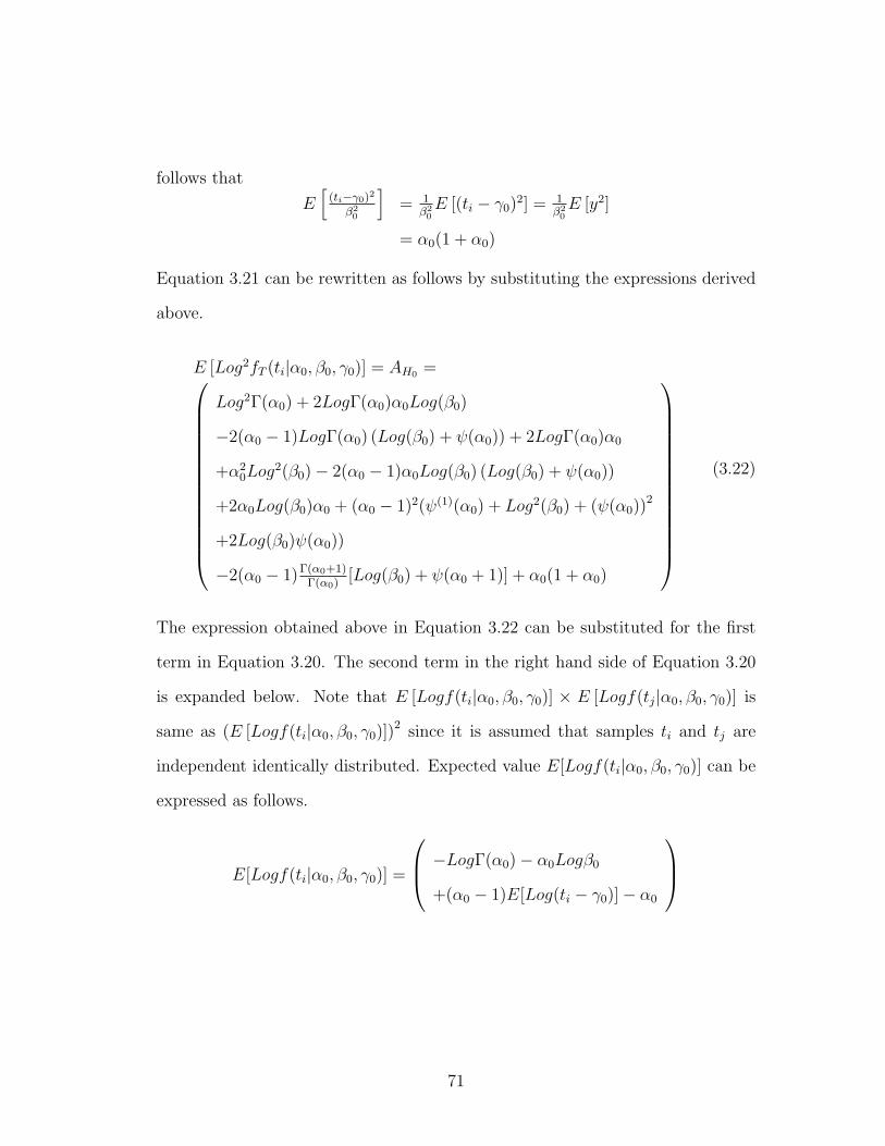
follows that

E[

(ti−γ0)2

β20

]= 1

β20E [(ti − γ0)2] = 1

β20E [y2]

= α0(1 + α0)

Equation 3.21 can be rewritten as follows by substituting the expressions derived

above.

E [Log2fT (ti|α0, β0, γ0)] = AH0 =


−2(α0 − 1)LogΓ(α0) (Log(β0) + ψ(α0)) + 2LogΓ(α0)α0

+α20Log

2(β0)− 2(α0 − 1)α0Log(β0) (Log(β0) + ψ(α0))

+2α0Log(β0)α0 + (α0 − 1)2(ψ(1)(α0) + Log2(β0) + (ψ(α0))2

+2Log(β0)ψ(α0))

−2(α0 − 1)Γ(α0+1)Γ(α0)

[Log(β0) + ψ(α0 + 1)] + α0(1 + α0)

(3.22)

The expression obtained above in Equation 3.22 can be substituted for the first

term in Equation 3.20. The second term in the right hand side of Equation 3.20

is expanded below. Note that E [Logf(ti|α0, β0, γ0)] × E [Logf(tj|α0, β0, γ0)] is

same as (E [Logf(ti|α0, β0, γ0)])2 since it is assumed that samples ti and tj are

independent identically distributed. Expected value E[Logf(ti|α0, β0, γ0)] can be

expressed as follows.

E[Logf(ti|α0, β0, γ0)] =

−LogΓ(α0)− α0Logβ0

+(α0 − 1)E[Log(ti − γ0)]− α0

71

Substituting the expression for E[Log(ti − γ0)] from Equation 3.14 the above

equation can be solved as follows.


(−LogΓ(α0)− Logβ0 + (α0 − 1)ψ(α0)− α0

)

(E[Logf(ti|α0, β0, γ0)])2 =(−LogΓ(α0)− Logβ0 + (α0 − 1)ψ(α0)− α0)×

(−LogΓ(α0)− Logβ0 + (α0 − 1)ψ(α0)− α0)

(E[Logf(ti|α0, β0, γ0)])2 = BH0 =

=

Log2Γ(α0) + 2LogΓ(α0)Logβ0

−2(α0 − 1)LogΓ(α0)ψ(α0) + 2α0LogΓ(α0)

+Log2β0 − 2(α0 − 1)Logβ0ψ(α0)

+2α0Logβ0 + (α0 − 1)2(ψ(α0))2

−2α0(α0 − 1)ψ(α0) + α20

(3.23)

The third term in Equation 3.20 is E [Log2fT (ti|α1, β1, γ1)] and it can be expanded

as follows.

E [Log2fT (ti|α1, β1, γ1)] =


−2(α1 − 1)LogΓ(α1)E [Log(ti − γ1)] + 2LogΓ(α1)E[ti−γ1

β1

]+α2

1Log2(β1)− 2(α1 − 1)α1Log(β1)E [Log(ti − γ1)]

+2α1Log(β1)E[ti−γ1

β1

]+ (α1 − 1)2E [Log2(ti − γ1)]

−2(α1 − 1)E[Log(ti − γ1) ti−γ1

β1

]+ E

[(ti−γ1)2

β21

]

(3.24)

Expressions for expected values in the right hand side of the above Equation 3.24

are listed below. The numerical solution to E[Log(ti − γ1)] is denoted by the

72

following (Equation 3.15).

E[Log(ti − γ1)] = I1(α0, β0, γ0, γ1)

Also, E[ti−γ1

β1

]can be expanded as follows.

E

[ti − γ1

β1

]=γ0 + α0β0 − γ1

β1

To the best of our knowledge, a closed form expression for E [Log2(ti − γ1)] cannot

be obtained. Numerical integration is used to find this expected value.

E [Log2(ti − γ1)] = 1Γ(α0)β

α00

∫∞γ0Log2(t− γ1)(t− γ0)(α0−1)e

− t−γ0β0 dt

= I2(α0, β0, γ0, γ1)

An expression for E [Log(ti − γ1)(ti − γ1)] can be obtained as follows.

E [Log(ti − γ1)(ti − γ1)] = E [Log(ti − γ1)((ti − γ0)− (γ1 − γ0))]

= E [Log(ti − γ1)(ti − γ0)]− (γ1 − γ0)E [Log(ti − γ1)]

= β0Γ(α0+1)

Γ(α0)I1(α0 + 1, β0, γ0, γ1)

−(γ1 − γ0)I1(α0, β0, γ0, γ1)

Expected value E[

(ti−γ1)2

β21

]can be expressed as follows.

E[

(ti−γ1)2

β21

]= E

[((ti−γ0)−(γ1−γ0))2

β21

]=

(α0(α0+1)β20+(γ1−γ0)2−2(γ1−γ0)α0β0)

β21

73

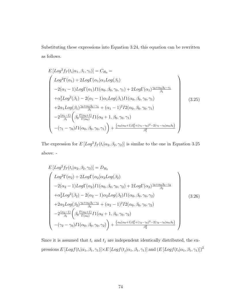
Substituting these expressions into Equation 3.24, this equation can be rewritten

as follows.

E [Log2fT (ti|α1, β1, γ1)] = CH0 =


−2(α1 − 1)LogΓ(α1)I1(α0, β0, γ0, γ1) + 2LogΓ(α1)γ0+α0β0−γ1

β1

+α21Log

2(β1)− 2(α1 − 1)α1Log(β1)I1(α0, β0, γ0, γ1)

+2α1Log(β1)γ0+α0β0−γ1

β1+ (α1 − 1)2I2(α0, β0, γ0, γ1)

−2 (α1−1)β1

(β0

Γ(α0+1)Γ(α0)

I1(α0 + 1, β0, γ0, γ1)

−(γ1 − γ0)I1(α0, β0, γ0, γ1)

)+

(α0(α0+1)β20+(γ1−γ0)2−2(γ1−γ0)α0β0)

β21

(3.25)

The expression for E [Log2fT (ti|α2, β2, γ2)] is similar to the one in Equation 3.25

above: -

E [Log2fT (ti|α2, β2, γ2)] = DH0



β2

+α22Log

2(β2)− 2(α2 − 1)α2Log(β2)I1(α0, β0, γ0, γ2)

+2α2Log(β2)γ0+α0β0−γ2

β2+ (α2 − 1)2I2(α0, β0, γ0, γ2)

−2 (α2−1)β2

(β0

Γ(α0+1)Γ(α0)

I1(α0 + 1, β0, γ0, γ2)

−(γ2 − γ0)I1(α0, β0, γ0, γ2)

)+

(α0(α0+1)β20+(γ2−γ0)2−2(γ2−γ0)α0β0)

β22

(3.26)

Since it is assumed that ti and tj are independent identically distributed, the ex-

pressions E [Logf(ti|α1, β1, γ1)]×E [Logf(tj|α1, β1, γ1)] and (E [Logf(ti|α1, β1, γ1)])2

74

are equivalent. Expected value E[Logf(ti|α1, β1, γ1)] can be expressed as follows.


−LogΓ(α1)− α1Logβ1

+(α1 − 1)E[Log(ti − γ1)]− E[ti−γ1

β1

]

or,

E[Logf(ti|α1, β1, γ1)] =(−LogΓ(α1)− α1Logβ1 + (α1 − 1)I1(α0, β0, γ0, γ1)− γ0+α0β0−γ1

β1

)

The expression (E[Logf(ti|α0, β0, γ0)])2 can then be written as follows.

(E[Logf(ti|α0, β0, γ0)])2 =

(−LogΓ(α1)− α1Logβ1 + (α1 − 1)I1(α0, β0, γ0, γ1)− γ0+α0β0−γ1

β1)×

(−LogΓ(α1)− α1Logβ1 + (α1 − 1)I1(α0, β0, γ0, γ1)− γ0+α0β0−γ1

β1)

Solving, there is the equality,

(E[Logf(ti|α1, β1, γ1)])2 = EH0 =

Log2Γ(α1) + 2α1LogΓ(α1)Logβ1


β1

+α21Log

2β1 − 2α1(α1 − 1)Logβ1I1(α0, β0, γ0, γ1)

+2α1Logβ1γ0+α0β0−γ1

β1+ (α1 − 1)2(I1(α0, β0, γ0, γ1))2

−2(α1 − 1)I1(α0, β0, γ0, γ1)γ0+α0β0−γ1

β1+(γ0+α0β0−γ1

β1

)2

(3.27)

75

The expression for (E[Logf(ti|α2, β2, γ2)])2 is similar to the expression above in

Equation 3.27.

(E[Logf(ti|α2, β2, γ2)])2 = FH0 =



β2

+α22Log

2β2 − 2α2(α2 − 1)Logβ2I1(α0, β0, γ0, γ2)


β2+ (α2 − 1)2(I1(α0, β0, γ0, γ2))2

−2(α2 − 1)I1(α0, β0, γ0, γ2)γ0+α0β0−γ2

β2+(γ0+α0β0−γ2

β2

)2

(3.28)

The expression E [Logf(ti|α0, β0, γ0)× Logf(ti|α1, β1, γ1)] can be expanded as fol-

lows.

E [Logf(ti|α0, β0, γ0)× Logf(ti|α1, β1, γ1)] =

E

LogΓ(α0)LogΓ(α1) + α1Logβ1LogΓ(α0)− LogΓ(α0)(α1 − 1)Log(ti − γ1)

+LogΓ(α0) ti−γ1

β1+ α0Logβ0LogΓ(α1) + α0α1Logβ0Logβ1

−α0Logβ0(α1 − 1)Log(ti − γ1) + α0Logβ0ti−γ1

β1

−(α0 − 1)Log(ti − γ0)LogΓ(α1)− α1(α0 − 1)Log(ti − γ0)Logβ1

+(α0 − 1)(α1 − 1)Log(ti − γ0)Log(ti − γ1)− (α0 − 1) ti−γ1

β1Log(ti − γ0)

+LogΓ(α1) ti−γ0

β0+ ti−γ0

β0α1Logβ1 − ti−γ0

β0(α1 − 1)Log(ti − γ1)

+(ti−γ0

β0

)(ti−γ1

β1

)

76

Solving, there is the equality

E [Logf(ti|α0, β0, γ0)× Logf(ti|α1, β1, γ1)] =

LogΓ(α0)LogΓ(α1) + α1Logβ1LogΓ(α0)

−LogΓ(α0)(α1 − 1)I1(α0, β0, γ0, γ1) + LogΓ(α0)γ0+α0β0−γ1

β1

+α0Logβ0LogΓ(α1) + α0α1Logβ0Logβ1

−α0Logβ0(α1 − 1)I1(α0, β0, γ0, γ1) + α0Logβ0γ0+α0β0−γ1

β1

−(α0 − 1) (Logβ0 + ψ(α0))LogΓ(α1)− α1(α0 − 1) (Logβ0 + ψ(α0))Logβ1

+(α0 − 1)(α1 − 1)E [Log(ti − γ0)Log(ti − γ1)]

−(α0 − 1)E[ti−γ1

β1Log(ti − γ0)

]+ LogΓ(α1)α0 + α0α1Logβ1

−(α1 − 1)E[ti−γ0

β0Log(ti − γ1)

]+ E

[(ti−γ0

β0

)(ti−γ1

β1

)]

(3.29)

A closed form expression for E [Log(ti − γ0)Log(ti − γ1)] is not available. A new

function is defined to represent the expected value that is obtained using numerical

integration.

E [Log(ti − γ0)Log(ti − γ1)] =

1Γ(α0)β

α00

∫∞γ0Log(ti − γ0)Log(ti − γ1)(ti − γ0)(α0−1)e

− ti−γ0β0 dti = I3(α0, β0, γ0, γ1)

Expressions for expected values E[(ti − γ1)Log(ti − γ0)], E[(ti − γ0)Log(ti − γ1)]

and E[(ti − γ0)(ti − γ1)] are as follows.

E[(ti−γ1)Log(ti−γ0)] =β0Γ(α0 + 1)

Γ(α0)(Logβ0+ψ(α0+1))−(γ1−γ0)(Logβ0+ψ(α0))

E[(ti − γ0)Log(ti − γ1)] =β0Γ(α0 + 1)

Γ(α0)I1(α0 + 1, β0, γ0, γ1)

E[(ti − γ0)(ti − γ1)] = α0β20(1 + α0)− α0β0(γ1 − γ0)

77

Substituting these values, Equation 3.29 can be rewritten as follows.

E [Logf(ti|α0, β0, γ0)× Logf(ti|α1, β1, γ1)] = GH0 =

LogΓ(α0)LogΓ(α1) + α1Logβ1LogΓ(α0)− LogΓ(α0)(α1 − 1)I1(α0, β0, γ0, γ1)

+LogΓ(α0)γ0+α0β0−γ1



β1


+(α0 − 1)(α1 − 1)I3(α0, β0, γ0, γ1)

−(α0 − 1)

(β0Γ(α0+1)


β1

)+ LogΓ(α1)α0

+α0α1Logβ1 − (α1 − 1)Γ(α0+1)Γ(α0)

I1(α0 + 1, β0, γ0, γ1) + α0β0(1+α0)−α0(γ1−γ0)β1

(3.30)

The expression for E [Logf(ti|α0, β0, γ0)× Logf(ti|α2, β2, γ2)] is similar to the ex-

pression in the Equation 3.30 above.

E [Logf(ti|α0, β0, γ0)× Logf(ti|α2, β2, γ2)] = HH0 =

LogΓ(α0)LogΓ(α2) + α2Logβ2LogΓ(α0)− LogΓ(α0)(α2 − 1)I1(α0, β0, γ0, γ2)




β2


+(α0 − 1)(α2 − 1)I3(α0, β0, γ0, γ2)

−(α0 − 1)

(β0Γ(α0+1)


β2

)+ LogΓ(α2)α0

+α0α2Logβ2 − (α2 − 1)Γ(α0+1)Γ(α0)

I1(α0 + 1, β0, γ0, γ2) + α0β0(1+α0)−α0(γ2−γ0)β2

(3.31)

The expression for E[Logf(ti|α0, β0, γ0)]×E[Logf(tj|α1, β1, γ1)] is the product

78

of the expressions for E[Logf(ti|α0, β0, γ0)] and E[Logf(tj|α1, β1, γ1)].


(−LogΓ(α0)− Logβ0 + (α0 − 1)ψ(α0)− α0

)

E[Logf(tj|α1, β1, γ1)] =(−LogΓ(α1)− α1Logβ1 + (α1 − 1)I1(α0, β0, γ0, γ1)− γ0+α0β0−γ1

β1

)

E[Logf(ti|α0, β0, γ0)]× E[Logf(tj|α1, β1, γ1)] = IH0 =

LogΓ(α0)LogΓ(α1) + α1LogΓ(α0)Logβ1 − LogΓ(α0)(α1 − 1)I1(α0, β0, γ0, γ1)


β1+ Logβ0LogΓ(α1) + Logβ0α1Logβ1

−Logβ0(α1 − 1)I1(α0, β0, γ0, γ1) + Logβ0γ0+α0β0−γ1

β1

−(α0 − 1)ψ(α0)LogΓ(α1)− (α0 − 1)ψ(α0)α1Logβ1

+(α0 − 1)ψ(α0)(α1 − 1)I1(α0, β0, γ0, γ1)− (α0 − 1)ψ(α0)γ0+α0β0−γ1

β1

+α0LogΓ(α1) + α0α1Logβ1 − α0(α1 − 1)I1(α0, β0, γ0, γ1) + α0γ0+α0β0−γ1

β1

(3.32)

The expression for E[Logf(ti|α0, β0, γ0)]× E[Logf(tj|α2, β2, γ2)] is similar to the

one above in Equation 3.32.

E[Logf(ti|α0, β0, γ0)]× E[Logf(tj|α2, β2, γ2)] = JH0 =

LogΓ(α0)LogΓ(α2) + α2LogΓ(α0)Logβ2 − LogΓ(α0)(α2 − 1)I1(α0, β0, γ0, γ2)


β2+ Logβ0LogΓ(α2) + Logβ0α2Logβ2

−Logβ0(α2 − 1)I1(α0, β0, γ0, γ2) + Logβ0γ0+α0β0−γ2

β2

−(α0 − 1)ψ(α0)LogΓ(α2)− (α0 − 1)ψ(α0)α2Logβ2

+(α0 − 1)ψ(α0)(α2 − 1)I1(α0, β0, γ0, γ2)− (α0 − 1)ψ(α0)γ0+α0β0−γ2

β2

+α0LogΓ(α2) + α0α2Logβ2 − α0(α2 − 1)I1(α0, β0, γ0, γ2) + α0γ0+α0β0−γ2

β2

(3.33)

The final expression needed to be substituted in Equation 3.20 is the one for

79

E[Logf(ti|α1, β1, γ1)] × E[Logf(tj|α2, β2, γ2)] and this expression is simply the

product of the expressions for E[Logf(ti|α1, β1, γ1)] and E[Logf(ti|α2, β2, γ2)].


β1

)


β2

)E[Logf(ti|α1, β1, γ1)]× E[Logf(tj|α2, β2, γ2)] = KH0 =

LogΓ(α1)LogΓ(α2) + LogΓ(α1)α2Logβ2 − LogΓ(α1)(α2 − 1)I1(α0, β0, γ0, γ2)


β2+ α1Logβ1LogΓ(α2) + α1Logβ1α2Logβ2


β2

−(α1 − 1)I1(α0, β0, γ0, γ1)LogΓ(α2)− (α1 − 1)I1(α0, β0, γ0, γ1)α2Logβ2

+(α1 − 1)I1(α0, β0, γ0, γ1)(α2 − 1)I1(α0, β0, γ0, γ2)

−(α1 − 1)I1(α0, β0, γ0, γ1)γ0+α0β0−γ2

β2+ γ0+α0β0−γ1

β1LogΓ(α2)

+γ0+α0β0−γ1

β1α2Logβ2 − γ0+α0β0−γ1

β1(α2 − 1)I1(α0, β0, γ0, γ2)

+γ0+α0β0−γ1

β1

γ0+α0β0−γ2

β2

(3.34)

The right hand side of Equation 3.20 can be rewritten as follows by using the

expressions obtained in Equations 3.22, 3.23, 3.25, 3.26, 3.27, 3.28, 3.30, 3.31,

3.32, 3.33 and 3.34.

E[L2] =

nAH0 + n(n− 1)BH0 + bn

2cCH0 + bn

2c(bn

2c − 1)EH0

+dn2eDH0 + dn

2e(dn

2e − 1)FH0 − 2bn

2cGH0 − 2bn

2c(n− 1)IH0

−2dn2eHH0 − 2dn

2e(n− 1)JH0 + 2bn

2cdn

2eKH0

(3.35)

80

This final expression for second moment of L when H0 is true and parameters are

in the L-finite subspace was validated using simulations and it accurately predicts

the second moment. Formal validation results are presented in Chapter 4 where

the expression obtained above in Equation 3.35 is used to obtain the receiver

operating characteristics.

3.4.4 Expected value: L-infinite

Recall that when parameters are in the L-infinite subspace, γ0 < Max(γ1, γ2),

and in this subspace L is finite with probability that given by Equation 3.7, and

is infinite with probability that is given by Equation 3.6. When parameters are

in L-infinite subspace, E[L] = ∞ because the probability of L being infinite is

nonzero. However, if the samples of L for which L is infinite are excluded and

only the samples for which L is finite are considered then the expected value of

L is finite. In this section, an expression for this expected value of L will be

derived given the conditions that the parameters are in the L-infinite subspace

and L is finite. Likelihood ratio L is finite when ti > Max(γ1, γ2),∀i : i ∈ {1..n}.

Samples ti are drawn from the Gamma distribution with parameters α0, β0 and

γ0. If the samples ti that have a value less than Max(γ1, γ2) are to be ignored

and all other samples are to be considered, then these samples have a truncated

Gamma probability density function. Define a new random variable Z that has

a truncated Gamma probability density function and all values less than some

constant ξ are truncated. The the PDF of Z is as follows

fZ(z) =

1K

1Γ(α)βα

(z − γ)α−1e−z−γβ z ≥ ξ

0 otherwise(3.36)

81

Where,

K =1

Γ(α)βα

∫ ∞ξ

(x− γ)α−1e−x−γβ dx (3.37)

Numerical integration will be used to find all the expected values that involve this

PDF. When H0 is true and only the RTT samples that have a value greater than

ξ (ξ ≥ γ0) are selected, then the functions defined below represent the expected

values can be obtained using numerical integration.

Ez(α0, β0, γ0, ξ) = E[z] =1

K

1

Γ(α0)βα00

∫ ∞ξ

z(z − γ0)α0−1e− z−γ0

β0 dz

Define

ELzMG(α0, β0, γ0, ξ, γ1) = E[Log(z − γ1)]

= 1K

1Γ(α0)β

α00

∫∞ξLog(z − γ1)(z − γ0)α0−1e

− z−γ0β0 dz

The expression for likelihood ratio can be rewritten as follows.

L = Log

∏bn2c

j=1fZ(zj|α0, β0, γ0)∏n

k=bn2c+1fZ(zk|α0, β0, γ0)∏bn

2c

j=1fZ(zj|α1, β1, γ1)∏n

k=bn2c+1fZ(zk|α2, β2, γ2)

(3.38)

The expression for E[L|H0] similar to the one in Section 3.4.2.

E[L|H0] = −nLog[Γ(α0)]− nα0Log[β0] + bn2c(α0 − 1)E[Log(zj − γ0)]

−bn2c (E[zj ]−γ0)

β0+ dn

2e(α0 − 1)E[Log(zk − γ0)]

−dn2e (E[zk]−γ0)

β0+ bn

2cLog[Γ(α1)] + bn

2cα1Log[β1]

−bn2c(α1 − 1)E[Log(zj − γ1)] + bn

2c (E[zj ]−γ1)

β1+ dn

2eLog[Γ(α2)]

+dn2eα2Log[β2]− dn

2e(α2 − 1)E[Log(zj − γ2)] + dn

2e (E[zj ]−γ2)

β2

(3.39)

Since closed form solutions to the various expressions in the right hand side of the

above equation are not known, numerical integration is used to obtain a value of

82

the above expression. Let ξ1 = Max(γ0, γ1) and ξ2 = Max(γ0, γ2). For L to be

finite, the samples zj, j ∈ {1..bn2 c} should all have a value that is greater than ξ1

and samples zk, k ∈ {bn2 c+1..n} should all be greater than ξ2. Hence, it is assumed

that zj’s are samples from a truncated Gamma distribution with parameters α0,

β0, γ0, truncated at ξ1 and zk’s are samples from truncated Gamma distribution

with the same parameters but truncated at ξ2.

E[L|H0] = −nLog[Γ(α0)]− nα0Log[β0]

+bn2c(α0 − 1)ELzMG(α0, β0, γ0, ξ1, γ0)

−bn2c (Ez(α0,β0,γ0,ξ1)−γ0)

β0+ dn

2e(α0 − 1)ELzMG(α0, β0, γ0, ξ2, γ0)

−dn2e (Ez(α0,β0,γ0,ξ2)−γ0)

β0+ bn

2cLog[Γ(α1)] + bn

2cα1Log[β1]

−bn2c(α1 − 1)ELzMG(α0, β0, γ0, ξ1, γ1) + bn

2c (Ez(α0,β0,γ0,ξ1)−γ1)

β1

+dn2eLog[Γ(α2)] + dn

2eα2Log[β2]

−dn2e(α2 − 1)ELzMG(α0, β0, γ0, ξ2, γ2) + dn

2e (Ez(α0,β0,γ0,ξ2)−γ2)

β2

(3.40)

The expression for expected value derived above in Equation 3.40 was validated

using simulations and it accurately predicts the expected value of L when param-

eters are in L-infinite subspace and only samples of L that have a finite value are

considered. Formal validation results are presented in chapter 4 where the ex-

pression obtained above in Equation 3.40 is used to predict the receiver operating

characteristics.

3.4.5 Second Moment: L-infinite

An expression for second moment of L when H0 is true and the parameters

are in the L-infinite subspace will be found in this section. The expression for

83

second moment can be written as follows.

E[L2] = E

∑bn

2c

j=1LogfZ(zj|α0, β0, γ0) +∑n

k=bn2c+1LogfZ(zk|α0, β0, γ0)

−∑bn

2c

j=1LogfZ(zj|α1, β1, γ1)−∑n

k=bn2c+1LogfZ(zk|α2, β2, γ2)

2

This expression can be expanded as follows.

E[L2] =

E

∑bn2c

j1=1

∑bn2c

j2=1(LogfZ(zj1|α0, β0, γ0))× (LogfZ(zj2|α0, β0, γ0))

+∑n

k1=bn2c+1

∑nk2=bn

2c+1(LogfZ(zk1|α0, β0, γ0))× (LogfZ(zk2|α0, β0, γ0))

+∑bn

2c

j1=1

∑bn2c


+∑n

k1=bn2c+1

∑nk2=bn

2c+1(LogfZ(zk1|α2, β2, γ2))× (LogfZ(zk2|α2, β2, γ2))

+2×∑bn

2c

j=1

∑nk=bn

2c+1(LogfZ(zj|α0, β0, γ0))× (LogfZ(zk|α0, β0, γ0))

−2×∑bn

2c

j1=1

∑bn2c


−2×∑bn

2c

j=1

∑nk=bn


−2×∑bn

2c

j=1

∑nk=bn


−2×∑n

k1=bn2c+1

∑nk2=bn

2c+1(LogfZ(zk1|α0, β0, γ0))×

(LogfZ(zk2|α2, β2, γ2))

+2×∑bn

2c

j=1

∑nk=bn


This equation can be expanded further by separating the terms for which zj1 =

zj2(or zk1 = zk2). Also, since it is assumed that zj1 (or zk1) and zj2 (or zk2) are

samples from independent identically distributed random variables, expressions of

the form E[u(zj1)v(zj2)] can be simplified as E[u(zj1)v(zj2)] = E[u(zj1)]E[v(zj2)],

where u and v are some functions. Here, zj’s and zk’s are samples from trun-

cated Gamma distribution with parameters α0, β0, γ0, truncated at ξ1 and ξ2

84

respectively.

E[L2] =

∑bn2c

j=1E [Log2fZ(zj|α0, β0, γ0)]

+∑bn

2c

j1=1

∑bn2c

j2=1,j26=j1E [LogfZ(zj1|α0, β0, γ0)]× E [LogfZ(zj2|α0, β0, γ0)]

+∑n

k=bn2c+1E [Log2fZ(zk|α0, β0, γ0)]

+∑n

k1=bn2c+1

∑nk2=bn

2c+1,k2 6=k1E [LogfZ(zk1|α0, β0, γ0)]×

E [LogfZ(zk2|α0, β0, γ0)]

+∑bn

2c

j=1E [Log2fZ(zj|α1, β1, γ1)]

+∑bn

2c

j1=1

∑bn2c


+∑n

k=bn2c+1E [Log2fZ(zk|α2, β2, γ2)]

+∑n

k1=bn2c+1

∑nk2=bn

2c+1,k2 6=k1E [LogfZ(zk1|α2, β2, γ2)]×


+2×∑bn

2c

j=1

∑nk=bn

2c+1E [LogfZ(zj|α0, β0, γ0)]× E [LogfZ(zk|α0, β0, γ0)]

−2×∑bn

2c

j=1E [(LogfZ(zj|α0, β0, γ0))× (LogfZ(zj|α1, β1, γ1))]

−2×∑bn

2c

j1=1

∑bn2c


−2×∑bn

2c

j=1

∑nk=bn


−2×∑bn

2c

j=1

∑nk=bn


−2×∑n

k=bn2c+1E [(LogfZ(zk|α0, β0, γ0))× (LogfZ(zk|α2, β2, γ2))]

−2×∑n

k1=bn2c+1

∑nk2=bn

2c+1,k26=k1E [LogfZ(zk1|α0, β0, γ0)]×


+2×∑bn

2c

j=1

∑nk=bn


(3.41)

85

Equation 3.41 above can be rewritten as follows: -

E[L2] =

bn2cE [Log2fZ(zj|α0, β0, γ0)]

+bn2c(bn

2c − 1)E [LogfZ(zj1|α0, β0, γ0)]× E [LogfZ(zj2|α0, β0, γ0)]

+dn2eE [Log2fZ(zk|α0, β0, γ0)]

+dn2e(dn

2e − 1)E [LogfZ(zk1|α0, β0, γ0)]× E [LogfZ(zk2|α0, β0, γ0)]

+bn2cE [Log2fZ(zj|α1, β1, γ1)]

+bn2c(bn



+dn2e(dn


+2bn2cdn

2eE [LogfZ(zj|α0, β0, γ0)]× E [LogfZ(zk|α0, β0, γ0)]

−2bn2cE [(LogfZ(zj|α0, β0, γ0))× (LogfZ(zj|α1, β1, γ1))]

−2bn2c(bn


−2bn2cdn


−2bn2cdn


−2dn2eE [(LogfZ(zk|α0, β0, γ0))× (LogfZ(zk|α2, β2, γ2))]

−2dn2e(dn


+2bn2cdn


(3.42)

Numerical methods are used to obtain a value for the above expression in Equa-

tion 3.42 because the samples z are from a truncated Gamma distribution and

closed form expressions for the expected values with this distribution are not

known. Although the summations have been removed in Equation 3.42, the sub-

scripts j and k in zj and zk have been retained because they represent samples

from two different distributions. The subscript j represents a sample from trun-

86

cated Gamma distribution truncated at ξ1 and subscript k represents the same

distribution truncated at ξ2. The values for the second moment from above equa-

tion obtained using numerical integration were validated using simulation and the

above method accurately predicts the second moment of L. Formal validation re-

sults are presented in chapter 4 where the expression obtained above in Equation

3.42 is used to predict the receiver operating characteristics.

3.5 Moments of L: H1 true

In this section, expressions for the first two moments of L when H1 is true are

derived. Just like in the case when H0 was true, here the base parameter space

is partitioned into two subspaces (L-finite, L-infinte) and the moments of L can

be found using different methods for each of the two subspaces. Section 3.5.1

discusses how parameter space is partitioned. The probability of L being finite

when parameters are in L-infinite subspace is also derived in Section 3.5.1. When

H1 is true, first bn2c samples have Gamma density with parameters α1, β1 and γ1

and the remaining dn2e samples have Gamma density with parameters α2, β2 and

γ2. The likelihood ratio function can be expressed as follows.

L = Log

∏bn2c

j=1fT (tj|α0, β0, γ0)∏n

k=bn2c+1fT (tk|α0, β0, γ0)∏bn

2c

j=1fT (tj|α1, β1, γ1)∏n

k=bn2c+1fT (tk|α2, β2, γ2)

(3.43)

Equation 3.43 will be used to derive expressions for expected value of L and

variance of L. Expected value and variance of L when parameters are in the

L-finite subspace are derived in Sections 3.5.2 and 3.5.3 respectively. Expected

value and variance of L when parameters are in L-infinite subspace are derived

in Sections 3.5.4 and 3.5.5 respectively.

87

3.5.1 Parameter subspaces: γ0 > Min(γ1, γ2) and γ0 ≤Min(γ1, γ2)

When γ0 ≤ Min(γ1, γ2), both L and its first two moments are finite and the

parameters are in L-finite subspace. When γ0 > Min(γ1, γ2), it is possible for L

to be −∞ and the parameters are in L-infinite subspace. When γ0 > Min(γ1, γ2)

and H1 is true, it may happen that one or more of the samples ti have a value

such that ti < γ0 and therefore L = −∞ (see Equation 3.43). For L to be finite

when γ0 > Min(γ1, γ2), all n samples should have a value that is greater than

or equal to γ0, i.e., ti ≥ γ0,∀i : i ∈ {1..n}. The probability of this happening

(P (ti > γ0,∀i : i ∈ {1..n})) can be evaluated as follows (assuming i.i.d.)

P (ti > γ0,∀i : i ∈ {1..n}) =

P(tj > γ0,∀j : j ∈

{1..⌊n2

⌋})× P

(tk > γ0,∀k : k ∈

{(⌊n2

⌋+ 1)..n})

Where

P(tj > γ0,∀j : j ∈

{1..⌊n

2

⌋})= P

(Min

[tj, j ∈

{1..bn

2c}]

> γ0

)

and

P(tk > γ0,∀k : k ∈

{(⌊n2

⌋+ 1)..n})

= P(Min

[tk, k ∈

{bn

2c+ 1..n

}]> γ0

)

Therefore,

P (ti > γ0,∀i : i ∈ {1..n}) =(P(Min

[tj, j ∈

{1..bn

2c}]

> γ0

))×(P(Min

[tk, k ∈

{bn

2c+ 1..n

}]> γ0

)) (3.44)

When Min(γ1, γ2) < γ0, then one of the following cases is true

88

• (γ1 < γ0) and (γ2 < γ0)

• (γ1 < γ0) and (γ2 ≥ γ0)

• (γ1 ≥ γ0) and (γ2 < γ0)

Using the PDF of the first order statistic (see section 3.4.1), the probability

P (ti > γ0,∀i : i ∈ {1..n}) can be evaluated as follows for each of the three cases.

• (γ1 < γ0) and (γ2 < γ0)

P (ti > γ0,∀i : i ∈ {1..n}) =(

bn/2c[Γ(α1)]bn/2cβ

α11

∫∞γ0−γ1

qα1−1e− qβ1

[Γ(α1,

qβ1

)]bn2c−1

dq

)×(

dn/2e[Γ(α2)]dn/2eβ

α22

∫∞γ0−γ2

qα2−1e− qβ2

[Γ(α2,

qβ2

)]dn2e−1

dq

) (3.45)

• (γ1 < γ0) and (γ2 ≥ γ0)

P (ti > γ0,∀i : i ∈ {1..n}) =(bn/2c

[Γ(α1)]bn/2cβα11

∫∞γ0−γ1

qα1−1e− qβ1

[Γ(α1,

qβ1

)]bn2c−1

dq

) (3.46)

• (γ1 ≥ γ0) and (γ2 < γ0)

P (ti > γ0,∀i : i ∈ {1..n}) =(dn/2e

[Γ(α2)]dn/2eβα22

∫∞γ0−γ2

qα2−1e− qβ2

[Γ(α2,

qβ2

)]dn2e−1

dq

) (3.47)

Hence, when Min(γ1, γ2) < γ0 and H1 is true, then probability that L is finite

is given by Equations 3.45, 3.46 and 3.47. These expressions will be used later

in Chapter 4 where expressions for probability of detection and false alarms are

derived. When γ0 ≤ Min(γ1, γ2), then L is finite and so are the first two moments.

89

An expression for the expected value of L when parameters are in L-finite subspace

will be obtained in the following section.

3.5.2 Expected Value: L-finite

In this section an expression for the expected value of L will be derived given

that H1 is true and γ0 ≤ Min(γ1, γ2) (L-finite). Solving Equation 3.43 can be

expressed as follows

L =

∑bn2c

j=1LogfT (tj|α0, β0, γ0) +∑n

k=bn2c+1LogfT (tk|α0, β0, γ0)

−∑bn

2c

j=1LogfT (tj|α1, β1, γ1)−∑n


Since ti > γ0,∀i : i ∈ {1..n}, from Equation 3.1 it follows that

L =

−bn2cLog(Γ(α0))− bn

2cα0Logβ0 + (α0 − 1)

∑bn2c

j=1Log(tj − γ0)

−∑bn

2c

j=1tj−γ0

β0− dn

2eLog(Γ(α0))− dn

2eα0Logβ0

+(α0 − 1)∑n

k=bn2c+1Log(tk − γ0)−

∑nk=bn

2c+1

tk−γ0

β0+ bn

2cLog(Γ(α1))

+bn2cα1Logβ1 − (α1 − 1)

∑bn2c

j=1Log(tj − γ1) +∑bn

2c

j=1tj−γ1

β1

+dn2eLog(Γ(α2)) + dn

2eα2Logβ2 − (α2 − 1)

∑nk=bn

2c+1Log(tk − γ2)

+∑n

k=bn2c+1

tk−γ2

β2

90

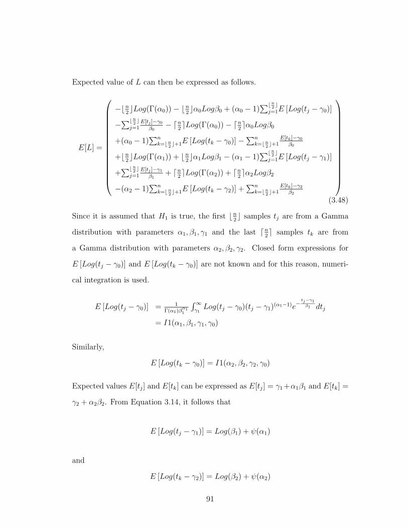
Expected value of L can then be expressed as follows.

E[L] =


2cα0Logβ0 + (α0 − 1)

∑bn2c

j=1E [Log(tj − γ0)]

−∑bn

2c

j=1E[tj ]−γ0

β0− dn


2eα0Logβ0

+(α0 − 1)∑n

k=bn2c+1E [Log(tk − γ0)]−

∑nk=bn

2c+1

E[tk]−γ0

β0

+bn2cLog(Γ(α1)) + bn

2cα1Logβ1 − (α1 − 1)

∑bn2c

j=1E [Log(tj − γ1)]

+∑bn

2c

j=1E[tj ]−γ1

β1+ dn

2eLog(Γ(α2)) + dn

2eα2Logβ2

−(α2 − 1)∑n

k=bn2c+1E [Log(tk − γ2)] +

∑nk=bn

2c+1

E[tk]−γ2

β2

(3.48)

Since it is assumed that H1 is true, the first bn2c samples tj are from a Gamma

distribution with parameters α1, β1, γ1 and the last dn2e samples tk are from

a Gamma distribution with parameters α2, β2, γ2. Closed form expressions for

E [Log(tj − γ0)] and E [Log(tk − γ0)] are not known and for this reason, numeri-

cal integration is used.

E [Log(tj − γ0)] = 1Γ(α1)β

α11

∫∞γ1Log(tj − γ0)(tj − γ1)(α1−1)e

−tj−γ1β1 dtj

= I1(α1, β1, γ1, γ0)

Similarly,

E [Log(tk − γ0)] = I1(α2, β2, γ2, γ0)

Expected values E[tj] and E[tk] can be expressed as E[tj] = γ1 +α1β1 and E[tk] =

γ2 + α2β2. From Equation 3.14, it follows that

E [Log(tj − γ1)] = Log(β1) + ψ(α1)

and

E [Log(tk − γ2)] = Log(β2) + ψ(α2)

91

The expressions obtained above can be substituted into Equation 3.48 to obtain

the following.

E[L] =


2cα0Logβ0 + bn

2c(α0 − 1)I1(α1, β1, γ1, γ0)

−bn2cγ1+α1β1−γ0

β0− dn


2eα0Logβ0

+dn2e(α0 − 1)I1(α2, β2, γ2, γ0)− dn

2eγ2+α2β2−γ0

β0+ bn

2cLog(Γ(α1))

+bn2cα1Logβ1 − bn2 c(α1 − 1)(Log(β1) + ψ(α1)) + bn

2cα1

+dn2eLog(Γ(α2)) + dn

2eα2Logβ2 − dn2 e(α2 − 1)(Log(β2) + ψ(α2))]

+dn2eα2

(3.49)

The equation 3.49 above was validated using simulation and it accurately predicts

the expected value of L when H1 is true. Formal validation results are presented

in Chapter 4 where the expression obtained above in Equation 3.49 is used to

predict the receiver operating characteristics.

3.5.3 Second Moment: L-finite

An expression for second moment of L when H1 is true and parameters are

in L-finite subspace will be obtained in this section. The second moment can be

derived from Equation 3.43 as follows.

E[L2] = E

Log ∏bn2 cj=1fT (tj|α0, β0, γ0)∏n

k=bn2c+1fT (tk|α0, β0, γ0)∏bn

2c

j=1fT (tj|α1, β1, γ1)∏n

k=bn2c+1fT (tk|α2, β2, γ2)

2This equation can be expanded as follows

E[L2] = E

∑bn

2c



−∑bn

2c



2

92

E[L2] =

E

∑bn2c



−∑bn

2c



× ∑bn2c



−∑bn

2c



E[L2] =

E

∑bn2c

j1=1

∑bn2c

j2=1(LogfT (tj1|α0, β0, γ0))× (LogfT (tj2|α0, β0, γ0))

+∑n

k1=bn2c+1

∑nk2=bn

2c+1(LogfT (tk1|α0, β0, γ0))× (LogfT (tk2|α0, β0, γ0))

+∑bn

2c

j1=1

∑bn2c


+∑n

k1=bn2c+1

∑nk2=bn

2c+1(LogfT (tk1|α2, β2, γ2))× (LogfT (tk2|α2, β2, γ2))

+2×∑bn

2c

j=1

∑nk=bn

2c+1(LogfT (tj|α0, β0, γ0))× (LogfT (tk|α0, β0, γ0))

−2×∑bn

2c

j1=1

∑bn2c


−2×∑bn

2c

j=1

∑nk=bn


−2×∑bn

2c

j=1

∑nk=bn


−2×∑n

k1=bn2c+1

∑nk2=bn

2c+1(LogfT (tk1|α0, β0, γ0))×

(LogfT (tk2|α2, β2, γ2))

+2×∑bn

2c

j=1

∑nk=bn


This equation can be expanded further by separating the terms for which tj1 =

tj2(or tk1 = tk2). Also, since it is assumed that tj1 (or tk1) and tj2 (or tk2) are

samples from independent distributions, expressions of the form E[u(tj1)v(tj2)]

can be simplified as E[u(tj1)v(tj2)] = E[u(tj1)]E[v(tj2)], where u and v are some

93

functions.

E[L2] =

∑bn2c

j=1E [Log2fT (tj|α0, β0, γ0)]

+∑bn

2c

j1=1

∑bn2c

j2=1,j26=j1E [LogfT (tj1|α0, β0, γ0)]× E [LogfT (tj2|α0, β0, γ0)]

+∑n

k=bn2c+1E [Log2fT (tk|α0, β0, γ0)]

+∑n

k1=bn2c+1

∑nk2=bn

2c+1,k2 6=k1E [LogfT (tk1|α0, β0, γ0)]×

E [LogfT (tk2|α0, β0, γ0)]

+∑bn

2c

j=1E [Log2fT (tj|α1, β1, γ1)]

+∑bn

2c

j1=1

∑bn2c


+∑n

k=bn2c+1E [Log2fT (tk|α2, β2, γ2)]

+∑n

k1=bn2c+1

∑nk2=bn

2c+1,k2 6=k1E [LogfT (tk1|α2, β2, γ2)]×

E [LogfT (tk2|α2, β2, γ2)]

+2×∑bn

2c

j=1

∑nk=bn

2c+1E [LogfT (tj|α0, β0, γ0)]× E [LogfT (tk|α0, β0, γ0)]

−2×∑bn

2c

j=1E [(LogfT (tj|α0, β0, γ0))× (LogfT (tj|α1, β1, γ1))]

−2×∑bn

2c

j1=1

∑bn2c


−2×∑bn

2c

j=1

∑nk=bn


−2×∑bn

2c

j=1

∑nk=bn


−2×∑n

k=bn2c+1E [(LogfT (tk|α0, β0, γ0))× (LogfT (tk|α2, β2, γ2))]

−2×∑n

k1=bn2c+1

∑nk2=bn

2c+1,k26=k1E [LogfT (tk1|α0, β0, γ0)]×

[LogfT (tk2|α2, β2, γ2)]

+2×∑bn

2c

j=1

∑nk=bn


(3.50)

94

Expressions of each of the terms on right hand side of equation 3.50 will now be

obtained. Expected value E[Log2fT (tj|α0, β0, γ0)] can be expressed as follows.

E[Log2fT (tj|α0, β0, γ0)] =

E

Log2Γ(α0) + α0LogΓ(α0)Logβ0

−LogΓ(α0)(α0 − 1)Log(tj − γ0) + LogΓ(α0)tj−γ0

β0

+α0Logβ0LogΓ(α0) + α20Log

2β0

−α0Logβ0(α0 − 1)Log(tj − γ0) + α0Logβ0tj−γ0

β0

−(α0 − 1)Log(tj − γ0)LogΓ(α0)

−(α0 − 1)Log(tj − γ0)α0Logβ0

+(α0 − 1)2Log2(tj − γ0)− (α0 − 1)Log(tj − γ0)tj−γ0

β0

+tj−γ0

β0LogΓ(α0) +

tj−γ0

β0α0Logβ0

− tj−γ0

β0(α0 − 1)Log(tj − γ0) +

(tj−γ0)2

β20

Which is the same as

E[Log2fT (tj|α0, β0, γ0)]

=


−2LogΓ(α0)(α0 − 1)E[Log(tj − γ0)] + 2LogΓ(α0)E[tj−γ0

β0

]+α2

0Log2β0 − 2α0Logβ0(α0 − 1)E[Log(tj − γ0)]

+2α0Logβ0E[tj−γ0

β0

]+ (α0 − 1)2E[Log2(tj − γ0)]

−2(α0 − 1)E[Log(tj − γ0)

tj−γ0

β0

]+ E

[(tj−γ0)2

β20

]

(3.51)

Since tj has Gamma density with parameters α1, β1 and γ1, it follows that

E[tj] = γ1 + α1β1

95

Closed form solutions to E[Log(tj − γ0)] and E[Log2(tj − γ0)] are not known and

these are solved numerically.

E[Log(tj − γ0)] = 1Γ(α1)β1

α1

∫∞γ1Log(tj − γ0)(tj − γ1)(α1−1)e

−tj−γ1β1 dtj

= I1(α1, β1, γ1, γ0)

E[Log2(tj − γ0)] = 1Γ(α1)β1

α1

∫∞γ1Log2(tj − γ0)(tj − γ1)(α1−1)e

−tj−γ1β1 dtj

= I2(α1, β1, γ1, γ0)

Expression for E[(tj−γ0)Log(tj−γ0)] and E[(tj−γ0)2] can be obtained by simple

algebraic manipulation as follows.

E[(tj − γ0)Log(tj − γ0)] = E [(tj − γ1)Log(tj − γ0)− (γ0 − γ1)Log(tj − γ0)]

= Γ(α1+1)Γ(α1)

β1I1(α1 + 1, β1, γ1, γ0)

−(γ0 − γ1)I1(α1, β1, γ1, γ0)

E[(tj − γ0)2] = E[((tj − γ1)− (γ0 − γ1))2]

= E[(tj − γ1)2] + (γ0 − γ1)2 − 2(γ0 − γ1)E[tj − γ1]

= β21α1(α1 + 1) + (γ0 − γ1)2 − 2(γ0 − γ1)α1β1

96

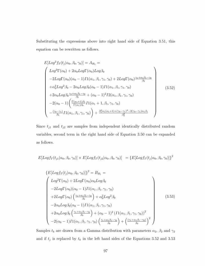
Substituting the expressions above into right hand side of Equation 3.51, this

equation can be rewritten as follows.

E[Log2fT (tj|α0, β0, γ0)] = AH1 =


−2LogΓ(α0)(α0 − 1)I1(α1, β1, γ1, γ0) + 2LogΓ(α0)γ1+α1β1−γ0

β0

+α20Log

2β0 − 2α0Logβ0(α0 − 1)I1(α1, β1, γ1, γ0)


β0+ (α0 − 1)2I2(α1, β1, γ1, γ0)

−2(α0 − 1)

(Γ(α1+1)β1

Γ(α1)β0I1(α1 + 1, β1, γ1, γ0)

− (γ0−γ1)β0

I1(α1, β1, γ1, γ0)

)+

β21α1(α1+1)+(γ0−γ1)2−2(γ0−γ1)α1β1

β20

(3.52)

Since tj1 and tj2 are samples from independent identically distributed random

variables, second term in the right hand side of Equation 3.50 can be expanded

as follows.

E[LogfT (tj1|α0, β0, γ0)]× E[LogfT (tj2|α0, β0, γ0)] = {E[LogfT (tj|α0, β0, γ0)]}2

{E[LogfT (tj|α0, β0, γ0)]}2 = BH1 =

Log2Γ(α0) + 2LogΓ(α0)α0Logβ0

−2LogΓ(α0)(α0 − 1)I1(α1, β1, γ1, γ0)

+2LogΓ(α0)(γ1+α1β1−γ0

β0

)+ α2

0Log2β0

−2α0Logβ0(α0 − 1)I1(α1, β1, γ1, γ0)

+2α0Logβ0

(γ1+α1β1−γ0

β0

)+ (α0 − 1)2 (I1(α1, β1, γ1, γ0))2

−2(α0 − 1)I1(α1, β1, γ1, γ0)(γ1+α1β1−γ0

β0

)+(

(γ1+α1β1−γ0)β0

)2

(3.53)

Samples tk are drawn from a Gamma distribution with parameters α2, β2 and γ2

and if tj is replaced by tk in the left hand sides of the Equations 3.52 and 3.53

97

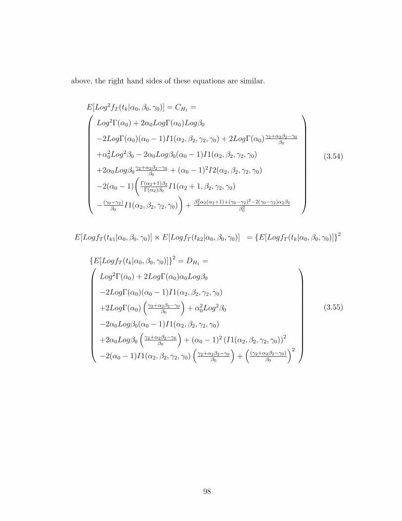
above, the right hand sides of these equations are similar.

E[Log2fT (tk|α0, β0, γ0)] = CH1 =


−2LogΓ(α0)(α0 − 1)I1(α2, β2, γ2, γ0) + 2LogΓ(α0)γ2+α2β2−γ0

β0

+α20Log

2β0 − 2α0Logβ0(α0 − 1)I1(α2, β2, γ2, γ0)


β0+ (α0 − 1)2I2(α2, β2, γ2, γ0)

−2(α0 − 1)

(Γ(α2+1)β2

Γ(α2)β0I1(α2 + 1, β2, γ2, γ0)

− (γ0−γ2)β0

I1(α2, β2, γ2, γ0)

)+

β22α2(α2+1)+(γ0−γ2)2−2(γ0−γ2)α2β2

β20

(3.54)

E[LogfT (tk1|α0, β0, γ0)]× E[LogfT (tk2|α0, β0, γ0)] = {E[LogfT (tk|α0, β0, γ0)]}2

{E[LogfT (tk|α0, β0, γ0)]}2 = DH1 =


−2LogΓ(α0)(α0 − 1)I1(α2, β2, γ2, γ0)

+2LogΓ(α0)(γ2+α2β2−γ0

β0

)+ α2

0Log2β0

−2α0Logβ0(α0 − 1)I1(α2, β2, γ2, γ0)

+2α0Logβ0

(γ2+α2β2−γ0

β0

)+ (α0 − 1)2 (I1(α2, β2, γ2, γ0))2

−2(α0 − 1)I1(α2, β2, γ2, γ0)(γ2+α2β2−γ0

β0

)+(

(γ2+α2β2−γ0)β0

)2

(3.55)

98

An expression for E[Log2fT (tj|α1, β1, γ1)] can be expanded as follows.

E[Log2fT (tj|α1, β1, γ1)] =


−2LogΓ(α1)(α1 − 1)E[Log(tj − γ1)] + 2LogΓ(α1)E[tj−γ1

β1

]+α2

1Log2β1 − 2α1Logβ1(α1 − 1)E[Log(tj − γ1)]

+2α1Logβ1E[tj−γ1

β1

]+ (α1 − 1)2E[Log2(tj − γ1)]

−2(α1 − 1)E[Log(tj − γ1)

tj−γ1

β1

]+ E

[(tj−γ1)2

β21

]

(3.56)

The following expected values can be obtained from the expressions that have

already been obtained previously in this chapter.

E[Log(tj − γ1)] = Logβ1 + ψ(α1)

E

[tj − γ1

β1

]= α1

E[Log2(tj − γ1)] = ψ(1)(α1) + Log2(β1) + (ψ(α1))2 + 2Log(β1)ψ(α1)

E

[Log(tj − γ1)

tj − γ1

β1

]=

Γ(α1 + 1)

Γ(α1)[Logβ1 + ψ(α1 + 1)]

E

[(tj − γ1)2

β21

]= α1(1 + α1)

99

Equation 3.56 can be rewritten as follows by substituting the expressions obtained

above.

E[Log2fT (tj|α1, β1, γ1)] = EH1 =


−2LogΓ(α1)(α1 − 1)(Logβ1 + ψ(α1)) + 2LogΓ(α1)α1

+α21Log

2β1 − 2α1Logβ1(α1 − 1)(Logβ1 + ψ(α1))

+2α1Logβ1α1 + (α1 − 1)2

(ψ(1)(α1) + Log2(β1)

+(ψ(α1))2 + 2Log(β1)ψ(α1)

)−2(α1 − 1)Γ(α1+1)

Γ(α1)[Logβ1 + ψ(α1 + 1)] + α1(1 + α1)

(3.57)

Since tj1 and tj2 are samples from independent identically distributed random

variables, it follows that.

E[LogfT (tj1|α1, β1, γ1)]× E[LogfT (tj2|α1, β1, γ1)] = {E[LogfT (tj|α1, β1, γ1)]}2

Expression for {E[LogfT (tj|α1, β1, γ1)]}2 is as follows.

{E[LogfT (tj|α1, β1, γ1)]}2 = FH1 =


−2LogΓ(α1)(α1 − 1)(Logβ1 + ψ(α1))

+2LogΓ(α1)α1 + α21Log

2β1

−2α1Logβ1(α1 − 1)(Logβ1 + ψ(α1))

+2α21Logβ1 + (α1 − 1)2(Logβ1 + ψ(α1))2

−2(α1 − 1)(Logβ1 + ψ(α1))α1 + α21

(3.58)

100

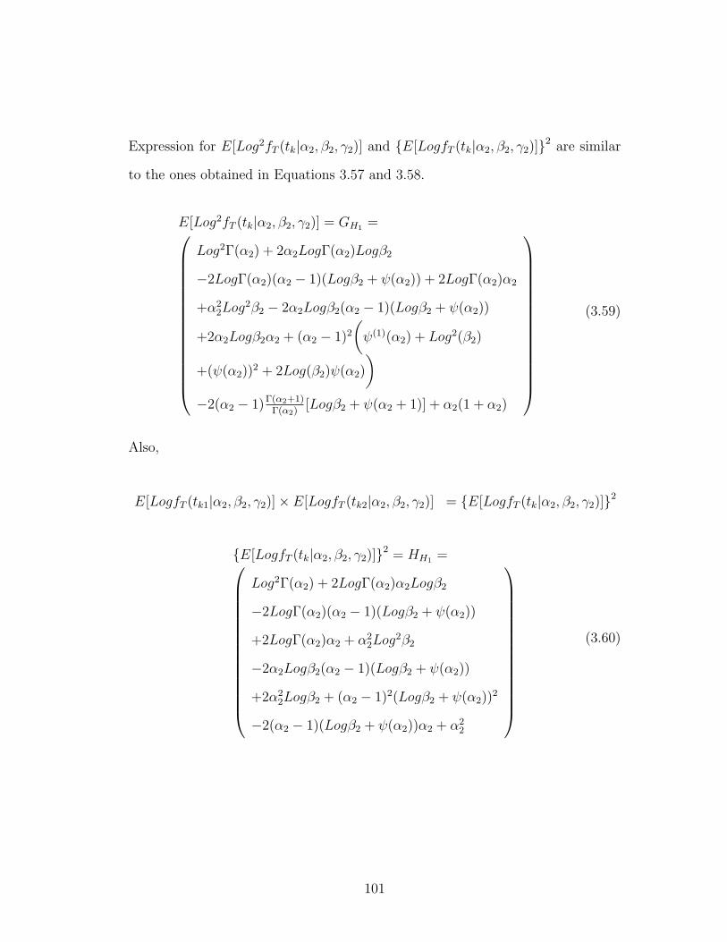
Expression for E[Log2fT (tk|α2, β2, γ2)] and {E[LogfT (tk|α2, β2, γ2)]}2 are similar

to the ones obtained in Equations 3.57 and 3.58.

E[Log2fT (tk|α2, β2, γ2)] = GH1 =


−2LogΓ(α2)(α2 − 1)(Logβ2 + ψ(α2)) + 2LogΓ(α2)α2

+α22Log

2β2 − 2α2Logβ2(α2 − 1)(Logβ2 + ψ(α2))

+2α2Logβ2α2 + (α2 − 1)2

(ψ(1)(α2) + Log2(β2)

+(ψ(α2))2 + 2Log(β2)ψ(α2)

)−2(α2 − 1)Γ(α2+1)

Γ(α2)[Logβ2 + ψ(α2 + 1)] + α2(1 + α2)

(3.59)

Also,

E[LogfT (tk1|α2, β2, γ2)]× E[LogfT (tk2|α2, β2, γ2)] = {E[LogfT (tk|α2, β2, γ2)]}2

{E[LogfT (tk|α2, β2, γ2)]}2 = HH1 =


−2LogΓ(α2)(α2 − 1)(Logβ2 + ψ(α2))

+2LogΓ(α2)α2 + α22Log

2β2

−2α2Logβ2(α2 − 1)(Logβ2 + ψ(α2))

+2α22Logβ2 + (α2 − 1)2(Logβ2 + ψ(α2))2

−2(α2 − 1)(Logβ2 + ψ(α2))α2 + α22

(3.60)

101

The expression for E[LogfT (tj|α0, β0, γ0)]×E[LogfT (tk|α0, β0, γ0)] can be obtained

as follows.

E[LogfT (tj|α0, β0, γ0)]× E[LogfT (tk|α0, β0, γ0)] =

E

Log2Γ(α0) + 2LogΓ(α0)α0Logβ0 − LogΓ(α0)(α0 − 1)Log(tk − γ0)

+LogΓ(α0)(tk−γ0

β0

)+ α2

0Log2β0 − α0Logβ0(α0 − 1)Log(tk − γ0)

+α0Logβ0

(tk−γ0

β0

)− LogΓ(α0)(α0 − 1)Log(tj − γ0)

−α0Logβ0(α0 − 1)Log(tj − γ0) + (α0 − 1)2Log(tj − γ0)Log(tk − γ0)

−(α0 − 1)Log(tj − γ0)(tk−γ0

β0

)+ LogΓ(α0)

(tj−γ0

β0

)+ α0Logβ0

(tj−γ0

β0

)−(tj−γ0

β0

)(α0 − 1)Log(tk − γ0) +

(tj−γ0

β0

)(tk−γ0

β0

)

E[LogfT (tj|α0, β0, γ0)]× E[LogfT (tk|α0, β0, γ0)] =

Log2Γ(α0) + 2LogΓ(α0)α0Logβ0 − LogΓ(α0)(α0 − 1)E[Log(tk − γ0)]

+LogΓ(α0)E[tk−γ0

β0

]+ α2

0Log2β0 − α0Logβ0(α0 − 1)E[Log(tk − γ0)]

+α0Logβ0E[tk−γ0

β0

]− LogΓ(α0)(α0 − 1)E[Log(tj − γ0)]

−α0Logβ0(α0 − 1)E[Log(tj − γ0)] + (α0 − 1)2E[Log(tj − γ0)Log(tk − γ0)]

−(α0 − 1)E[Log(tj − γ0)

(tk−γ0

β0

)]+ LogΓ(α0)E

[tj−γ0

β0

]+ α0Logβ0E

[tj−γ0

β0

]−(α0 − 1)E

[(tj−γ0

β0

)Log(tk − γ0)

]+ E

[(tj−γ0

β0

)(tk−γ0

β0

)]

(3.61)

The terms in the right hand side of Equation 3.61 can be expressed as follows.

E[Log(tj − γ0)] = I1(α1, β1, γ1, γ0)

E[Log(tk − γ0)] = I1(α2, β2, γ2, γ0)

E

[tj − γ0

β0

]=γ1 + α1β1 − γ0

β0

102

E

[tk − γ0

β0

]=γ2 + α2β2 − γ0

β0

Equation 3.61 can be rewritten as follows by substituting the expressions above.

E[LogfT (tj|α0, β0, γ0)]× E[LogfT (tk|α0, β0, γ0)] = IH1 =

Log2Γ(α0) + 2LogΓ(α0)α0Logβ0 − LogΓ(α0)(α0 − 1)I1(α2, β2, γ2, γ0)

+LogΓ(α0)(γ2+α2β2−γ0

β0

)+ α2

0Log2β0 − α0Logβ0(α0 − 1)I1(α2, β2, γ2, γ0)

+α0Logβ0

(γ2+α2β2−γ0

β0

)− LogΓ(α0)(α0 − 1)I1(α1, β1, γ1, γ0)

−α0Logβ0(α0 − 1)I1(α1, β1, γ1, γ0)

+(α0 − 1)2I1(α1, β1, γ1, γ0)I1(α2, β2, γ2, γ0)

−(α0 − 1)I1(α1, β1, γ1, γ0)(γ2+α2β2−γ0

β0

)+ LogΓ(α0)

(γ1+α1β1−γ0

β0

)+α0Logβ0

(γ1+α1β1−γ0

β0

)− (α0 − 1)

(γ1+α1β1−γ0

β0

)I1(α2, β2, γ2, γ0)

+(γ1+α1β1−γ0

β0

)(γ2+α2β2−γ0

β0

)

(3.62)

The expression for E[LogfT (tj|α0, β0, γ0) × LogfT (tj|α1, β1, γ1)] can be obtained

as follows.

E[LogfT (tj|α0, β0, γ0)× LogfT (tj|α1, β1, γ1)] =

E

LogΓ(α0)LogΓ(α1) + LogΓ(α0)α1Logβ1 − LogΓ(α0)(α1 − 1)Log(tj − γ1)

+LogΓ(α0)(tj−γ1

β1

)+ α0Logβ0LogΓ(α1) + α0Logβ0α1Logβ1

−α0Logβ0(α1 − 1)Log(tj − γ1) + α0Logβ0

(tj−γ1

β1

)−(α0 − 1)Log(tj − γ0)LogΓ(α1)− (α0 − 1)Log(tj − γ0)α1Logβ1

+(α0 − 1)Log(tj − γ0)(α1 − 1)Log(tj − γ1)

−(α0 − 1)Log(tj − γ0)(tj−γ1

β1

)+(tj−γ0

β0

)LogΓ(α1) +

(tj−γ0

β0

)α1Logβ1

−(tj−γ0

β0

)(α1 − 1)Log(tj − γ1) +

(tj−γ0

β0

)(tj−γ1

β1

)

103

E[LogfT (tj|α0, β0, γ0)× LogfT (tj|α1, β1, γ1)] =

LogΓ(α0)LogΓ(α1) + LogΓ(α0)α1Logβ1 − LogΓ(α0)(α1 − 1)E[Log(tj − γ1)]

+LogΓ(α0)E[tj−γ1

β1

]+ α0Logβ0LogΓ(α1) + α0Logβ0α1Logβ1

−α0Logβ0(α1 − 1)E[Log(tj − γ1)] + α0Logβ0E[tj−γ1

β1

]−(α0 − 1)E[Log(tj − γ0)]LogΓ(α1)− (α0 − 1)E[Log(tj − γ0)]α1Logβ1

+(α0 − 1)(α1 − 1)E[Log(tj − γ0)Log(tj − γ1)]

−(α0 − 1)E[Log(tj − γ0)

(tj−γ1

β1

)]+ E

[tj−γ0

β0

]LogΓ(α1)

+E[tj−γ0

β0

]α1Logβ1 − (α1 − 1)E

[(tj−γ0

β0

)Log(tj − γ1)

]+E

[(tj−γ0

β0

)(tj−γ1

β1

)]

(3.63)

The following expressions can be substituted into the right hand side of Equation

3.63.

E[log(tj − γ1)] = Logβ1 + ψ(α1)

E

[tj − γ1

β1

]= α1

E

[tj − γ0

β0

]=

(γ1 + α1β1 − γ0

β1

)E[Log(tj − γ0)] = I1(α1, β1, γ1, γ0)

E[Log(tj − γ0)Log(tj − γ1)] =

1Γ(α1)β

α11

∫∞γ1Log(tj − γ0)Log(tj − γ1)(tj − γ1)(α1−1)e

−tj−γ1β1 dtj

= I3(α1, β1, γ1, γ0)

E[(tj − γ1)Log(tj − γ0)] =Γ(α1 + 1)β1

Γ(α1)I1(α1 + 1, β1, γ1, γ0)

E[(tj−γ0)Log(tj−γ1)] =β1Γ(α1 + 1)


E[(tj − γ0)(tj − γ1)] = α1β21(1 + α1)− (γ0 − γ1)α1β1

104

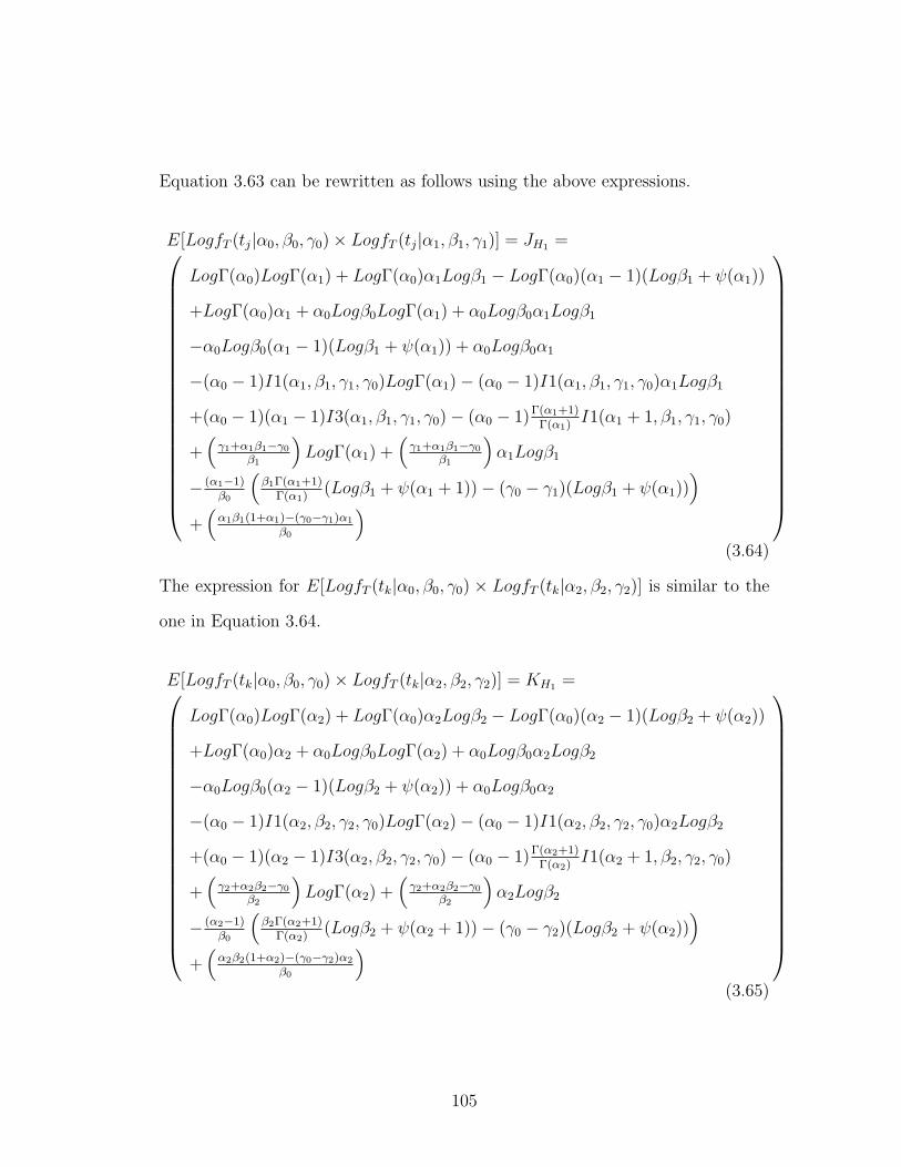
Equation 3.63 can be rewritten as follows using the above expressions.

E[LogfT (tj|α0, β0, γ0)× LogfT (tj|α1, β1, γ1)] = JH1 =

LogΓ(α0)LogΓ(α1) + LogΓ(α0)α1Logβ1 − LogΓ(α0)(α1 − 1)(Logβ1 + ψ(α1))

+LogΓ(α0)α1 + α0Logβ0LogΓ(α1) + α0Logβ0α1Logβ1

−α0Logβ0(α1 − 1)(Logβ1 + ψ(α1)) + α0Logβ0α1


+(α0 − 1)(α1 − 1)I3(α1, β1, γ1, γ0)− (α0 − 1)Γ(α1+1)Γ(α1)

I1(α1 + 1, β1, γ1, γ0)

+(γ1+α1β1−γ0

β1

)LogΓ(α1) +

(γ1+α1β1−γ0

β1

)α1Logβ1

− (α1−1)β0

(β1Γ(α1+1)

Γ(α1)(Logβ1 + ψ(α1 + 1))− (γ0 − γ1)(Logβ1 + ψ(α1))

)+(α1β1(1+α1)−(γ0−γ1)α1

β0

)

(3.64)

The expression for E[LogfT (tk|α0, β0, γ0) × LogfT (tk|α2, β2, γ2)] is similar to the

one in Equation 3.64.

E[LogfT (tk|α0, β0, γ0)× LogfT (tk|α2, β2, γ2)] = KH1 =


+LogΓ(α0)α2 + α0Logβ0LogΓ(α2) + α0Logβ0α2Logβ2



+(α0 − 1)(α2 − 1)I3(α2, β2, γ2, γ0)− (α0 − 1)Γ(α2+1)Γ(α2)

I1(α2 + 1, β2, γ2, γ0)

+(γ2+α2β2−γ0

β2

)LogΓ(α2) +

(γ2+α2β2−γ0

β2

)α2Logβ2

− (α2−1)β0

(β2Γ(α2+1)

Γ(α2)(Logβ2 + ψ(α2 + 1))− (γ0 − γ2)(Logβ2 + ψ(α2))

)+(α2β2(1+α2)−(γ0−γ2)α2

β0

)

(3.65)

105

The expression for E[LogfT (tj1|α0, β0, γ0)] × E[LogfT (tj2|α1, β1, γ1)] can be ob-

tained from the expressions for E[LogfT (tj1|α0, β0, γ0)] andE[LogfT (tj2|α1, β1, γ1)]

as follows.

E[LogfT (tj1|α0, β0, γ0)] =

−LogΓ(α0)− α0Logβ0 + (α0 − 1)I1(α1, β1, γ1)

−(γ1+α1β1−γ0

β0

)

E[LogfT (tj2|α1, β1, γ1)] =(−LogΓ(α1)− α1Logβ1 + (α1 − 1)(Logβ1 + ψ(α1))− α1

)

E[LogfT (tj1|α0, β0, γ0)× LogfT (tj2|α1, β1, γ1)] = LH1 =


+α1LogΓ(α0) + α0Logβ0LogΓ(α1) + α0Logβ0α1Logβ1



+(α0 − 1)I1(α1, β1, γ1, γ0)(α1 − 1)(Logβ1 + ψ(α1))

−(α0 − 1)I1(α1, β1, γ1, γ0)α1 +(γ1+α1β1−γ0

β0

)LogΓ(α1)

+(γ1+α1β1−γ0

β0

)α1Logβ1 −

(γ1+α1β1−γ0

β0

)(α1 − 1)(Logβ1 + ψ(α1))

+(γ1+α1β1−γ0

β0

)α1

(3.66)

106

The expression for E[LogfT (tk1|α0, β0, γ0)×LogfT (tk2|α2, β2, γ2)] is similar to the

one in Equation 3.66 above.

E[LogfT (tk1|α0, β0, γ0)× LogfT (tk2|α2, β2, γ2)] = MH1 =





+(α0 − 1)I1(α2, β2, γ2, γ0)(α2 − 1)(Logβ2 + ψ(α2))

−(α0 − 1)I1(α2, β2, γ2, γ0)α2 +(γ2+α2β2−γ0

β0

)LogΓ(α2)

+(γ2+α2β2−γ0

β0

)α2Logβ2 −

(γ2+α2β2−γ0

β0

)(α2 − 1)(Logβ2 + ψ(α2))

+(γ2+α2β2−γ0

β0

)α2

(3.67)

The expression for E[LogfT (tj|α0, β0, γ0) × LogfT (tk|α2, β2, γ2)] can be obtained

similarly and is as follows.

E[LogfT (tj|α0, β0, γ0)× LogfT (tk|α2, β2, γ2)] = NH1 =





+(α0 − 1)I1(α1, β1, γ1, γ0)(α2 − 1)(Logβ2 + ψ(α2))

−(α0 − 1)I1(α1, β1, γ1, γ0)α2

+(γ1+α1β1−γ0

β0

)LogΓ(α2) +

(γ1+α1β1−γ0

β0

)α2Logβ2

−(γ1+α1β1−γ0

β0

)(α2 − 1)(Logβ2 + ψ(α2)) +

(γ1+α1β1−γ0

β0

)α2

(3.68)

107

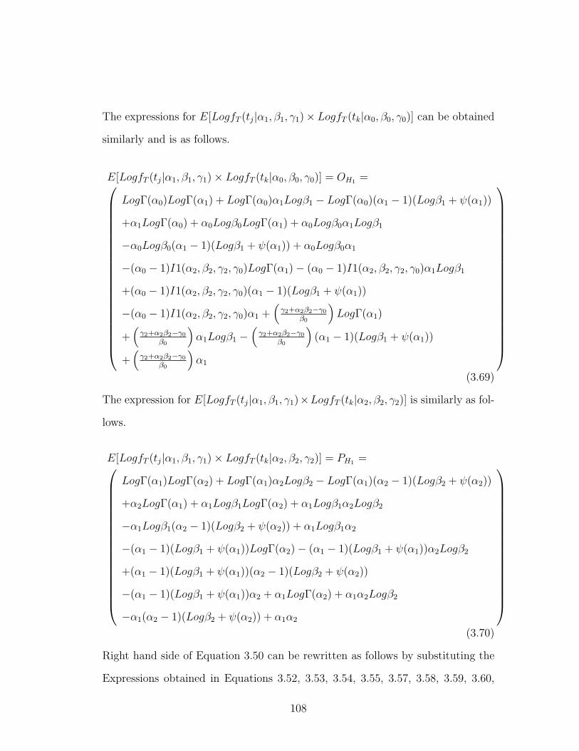
The expressions for E[LogfT (tj|α1, β1, γ1)×LogfT (tk|α0, β0, γ0)] can be obtained

similarly and is as follows.

E[LogfT (tj|α1, β1, γ1)× LogfT (tk|α0, β0, γ0)] = OH1 =





+(α0 − 1)I1(α2, β2, γ2, γ0)(α1 − 1)(Logβ1 + ψ(α1))

−(α0 − 1)I1(α2, β2, γ2, γ0)α1 +(γ2+α2β2−γ0

β0

)LogΓ(α1)

+(γ2+α2β2−γ0

β0

)α1Logβ1 −

(γ2+α2β2−γ0

β0

)(α1 − 1)(Logβ1 + ψ(α1))

+(γ2+α2β2−γ0

β0

)α1

(3.69)

The expression for E[LogfT (tj|α1, β1, γ1)×LogfT (tk|α2, β2, γ2)] is similarly as fol-

lows.

E[LogfT (tj|α1, β1, γ1)× LogfT (tk|α2, β2, γ2)] = PH1 =




−(α1 − 1)(Logβ1 + ψ(α1))LogΓ(α2)− (α1 − 1)(Logβ1 + ψ(α1))α2Logβ2

+(α1 − 1)(Logβ1 + ψ(α1))(α2 − 1)(Logβ2 + ψ(α2))

−(α1 − 1)(Logβ1 + ψ(α1))α2 + α1LogΓ(α2) + α1α2Logβ2

−α1(α2 − 1)(Logβ2 + ψ(α2)) + α1α2

(3.70)

Right hand side of Equation 3.50 can be rewritten as follows by substituting the

Expressions obtained in Equations 3.52, 3.53, 3.54, 3.55, 3.57, 3.58, 3.59, 3.60,

108

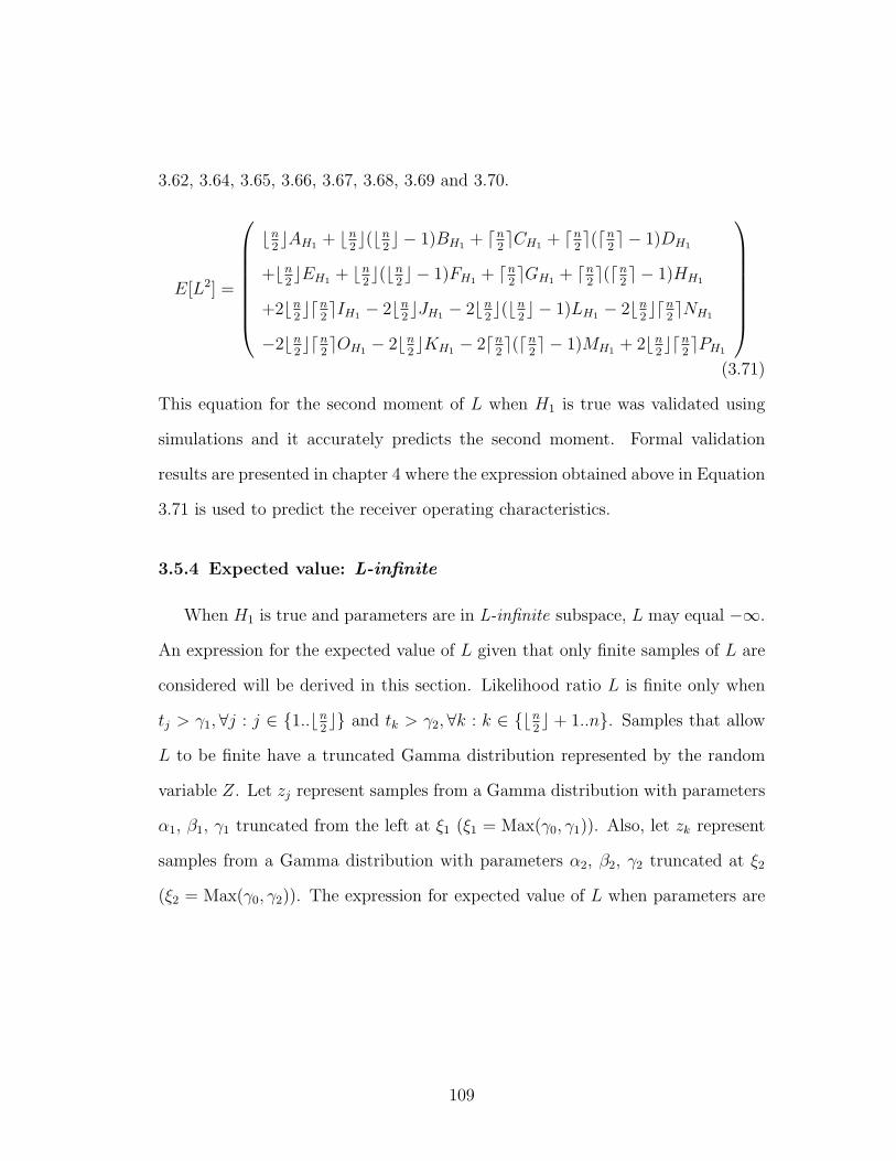
3.62, 3.64, 3.65, 3.66, 3.67, 3.68, 3.69 and 3.70.

E[L2] =

bn2cAH1 + bn

2c(bn

2c − 1)BH1 + dn

2eCH1 + dn

2e(dn

2e − 1)DH1

+bn2cEH1 + bn

2c(bn

2c − 1)FH1 + dn

2eGH1 + dn

2e(dn

2e − 1)HH1

+2bn2cdn

2eIH1 − 2bn

2cJH1 − 2bn

2c(bn

2c − 1)LH1 − 2bn

2cdn

2eNH1

−2bn2cdn

2eOH1 − 2bn

2cKH1 − 2dn

2e(dn

2e − 1)MH1 + 2bn

2cdn

2ePH1

(3.71)

This equation for the second moment of L when H1 is true was validated using

simulations and it accurately predicts the second moment. Formal validation

results are presented in chapter 4 where the expression obtained above in Equation

3.71 is used to predict the receiver operating characteristics.

3.5.4 Expected value: L-infinite

When H1 is true and parameters are in L-infinite subspace, L may equal −∞.

An expression for the expected value of L given that only finite samples of L are

considered will be derived in this section. Likelihood ratio L is finite only when

tj > γ1,∀j : j ∈ {1..bn2c} and tk > γ2,∀k : k ∈ {bn

2c + 1..n}. Samples that allow

L to be finite have a truncated Gamma distribution represented by the random

variable Z. Let zj represent samples from a Gamma distribution with parameters

α1, β1, γ1 truncated from the left at ξ1 (ξ1 = Max(γ0, γ1)). Also, let zk represent

samples from a Gamma distribution with parameters α2, β2, γ2 truncated at ξ2

(ξ2 = Max(γ0, γ2)). The expression for expected value of L when parameters are

109

in L-infinite subspace and L is finite can be written as follows.

E[L] =

∑bn2c

j=1E[LogfZ(zj|α0, β0, γ0)] +∑n

k=bn2c+1E[LogfZ(zk|α0, β0, γ0)]

−∑bn

2c

j=1E[LogfZ(zj|α1, β1, γ1)]−∑n

k=bn2c+1E[LogfZ(zk|α2, β2, γ2)]

(3.72)

This expression can be rewritten as follows.

E[L] =

bn2 cE[LogfZ(zj|α0, β0, γ0)] + dn2eE[LogfZ(zk|α0, β0, γ0)]

−bn2cE[LogfZ(zj|α1, β1, γ1)]− dn

2eE[LogfZ(zk|α2, β2, γ2)]

(3.73)

Since zj’s and zk’s are samples from a truncated Gamma distribution, it is very

difficult to obtain closed form solution for E[L]. Equation 3.73 is numerically

evaluated to obtain a value for E[L]. The values obtained using numerical methods

were validated using simulation and this method accurately predicts E[L] when

parameters are in L-infinite subspace and L is finite. Formal validation results

are presented in chapter 4 where the expression obtained above in Equation 3.73

is used to predict the receiver operating characteristics.

3.5.5 Second moment L-infinite

The expression for second moment of L when H1 is true, parameters are in

L-infinite subspace and L is finite is the same as the expression in Equation 3.42.

This equation is rewritten here for convenience. In the following equation, zk’s

represent samples from Gamma distribution with parameters α1, β1, γ1, truncated

at ξ1 and zk’s represent samples from Gamma distribution with parameters α2,

110

β2, γ2, truncated at ξ2.

E[L2] =

bn2cE [Log2fZ(zj|α0, β0, γ0)]

+bn2c(bn



+dn2e(dn


+bn2cE [Log2fZ(zj|α1, β1, γ1)]

+bn2c(bn



+dn2e(dn


+2bn2cdn


−2bn2cE [(LogfZ(zj|α0, β0, γ0))× (LogfZ(zj|α1, β1, γ1))]

−2bn2c(bn


−2bn2cdn


−2bn2cdn


−2dn2eE [(LogfZ(zk|α0, β0, γ0))× (LogfZ(zk|α2, β2, γ2))]

−2dn2e(dn


+2bn2cdn


(3.74)

It is difficult to obtain closed form expressions with truncated Gamma distri-

bution. Numerical methods were used to determine E[L2] from Equation 3.74.

The values predicted using numerical methods match the values obtained using

simulation. Formal validation results are presented in chapter 4 where the ex-

pression obtained above in Equation 3.74 is used to predict the receiver operating

characteristics.

111

3.6 Summary

Parameter unaware detector, that can be used to detect route changes was

proposed in this chapter in section 3.2. Since PUD is unaware of the Gamma

distribution parameters, it estimates these parameters from the RTT samples.

These parameter estimates are then used together with the RTT samples to find

the value of the likelihood ratio. Since parameter estimates (and not the actual

parameters) are used in the likelihood ratio function, it is currently not possible to

obtain expressions for moments of likelihood ratio for each of the two hypothesis.

Expressions for the PDF of the likelihood ratio for each of the two hypothesis

are needed to map the system parameters to probabilities of detection and false

alarms. Parameter aware detector was discussed in section 3.3. The PAD is the

optimal detector and it provides the theoretical upper bound on the best perfor-

mance that can be achieved by any detector. Since PAD uses known parameter

values in the likelihood ratio test (and not parameter estimates), expressions for

the first two moments of likelihood ratio can be obtained for PAD as discussed in

sections 3.4 and 3.5. These expressions for the first two moments of the likelihood

ratio will be used in chapter 4 to obtain receiver operating characteristics of PAD.

To derive the expressions for the first two moments of L for the PAD, the

base parameter space was divided into L-finite and L-infinite subspaces in both

cases (i.e., H0 true and H1 true). When parameters are in L-finite subspace, L

is always finite and expressions for the first two moments for this case were ob-

tained in Sections 3.4.2, 3.4.3, 3.5.2 and 3.5.3. When parameters are in L-infinite

subspace, likelihood ratio L may be either finite or infinite. The probability that

likelihood ratio is finite when parameters are in L-infinite subspace was derived in

sections 3.4.1 and 3.5.1. Given the conditions that the parameters are in L-infinite

112

subspace and L is finite, expressions for the first two moments of L were obtained

in sections 3.4.4, 3.4.5, 3.5.4 and 3.5.5. All of these expressions derived in this

chapter combined with the assumption that the conditional PDFs are Gaussian

will be used in Chapter 4 which validates this analysis and used to obtain receiver

operating characteristics of PAD.

113

Chapter 4

Model-Based Approach:

Validation

4.1 Introduction

The parameter aware detector or the ideal detector was introduced in the pre-

vious chapter. The first two moments of L for PAD, when hypothesis H0 is true

and hypothesis H1 is true were derived in sections 3.4 and 3.5 respectively. In

this chapter, these expressions for the first two moments of L combined with a

distribution assumption will be used to predict the probabilities of detection and

false alarm. Receiver operating characteristics (ROCs) will also be plotted for

various values of the parameters to illustrate PADs performance over the entire

range of thresholds. ROCs predicted using the analytical expressions will also be

compared to ROCs obtained using simulation. This will validate the expressions

for first two moments of L obtained in the previous chapter and also the expres-

sions for probabilities of detection and false alarm that will be obtained in this

chapter. Expressions for probability of false alarm and detection are obtained in

114

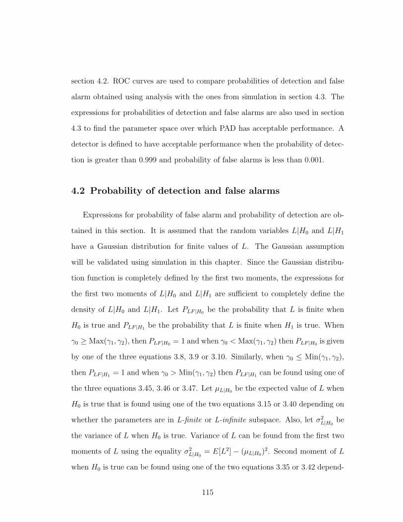
section 4.2. ROC curves are used to compare probabilities of detection and false

alarm obtained using analysis with the ones from simulation in section 4.3. The

expressions for probabilities of detection and false alarms are also used in section

4.3 to find the parameter space over which PAD has acceptable performance. A

detector is defined to have acceptable performance when the probability of detec-

tion is greater than 0.999 and probability of false alarms is less than 0.001.

4.2 Probability of detection and false alarms

Expressions for probability of false alarm and probability of detection are ob-

tained in this section. It is assumed that the random variables L|H0 and L|H1

have a Gaussian distribution for finite values of L. The Gaussian assumption

will be validated using simulation in this chapter. Since the Gaussian distribu-

tion function is completely defined by the first two moments, the expressions for

the first two moments of L|H0 and L|H1 are sufficient to completely define the

density of L|H0 and L|H1. Let PLF |H0 be the probability that L is finite when

H0 is true and PLF |H1 be the probability that L is finite when H1 is true. When

γ0 ≥ Max(γ1, γ2), then PLF |H0 = 1 and when γ0 < Max(γ1, γ2) then PLF |H0 is given

by one of the three equations 3.8, 3.9 or 3.10. Similarly, when γ0 ≤ Min(γ1, γ2),

then PLF |H1 = 1 and when γ0 > Min(γ1, γ2) then PLF |H1 can be found using one of

the three equations 3.45, 3.46 or 3.47. Let µL|H0 be the expected value of L when

H0 is true that is found using one of the two equations 3.15 or 3.40 depending on

whether the parameters are in L-finite or L-infinite subspace. Also, let σ2L|H0

be

the variance of L when H0 is true. Variance of L can be found from the first two

moments of L using the equality σ2L|H0

= E[L2]− (µL|H0)2. Second moment of L

when H0 is true can be found using one of the two equations 3.35 or 3.42 depend-

115

ing on whether the parameters are in L-finite or L-infinite subspace. Similarly,

let µL|H1 and σ2L|H1

represent the first moment and the variance of L when H1 is

true. Let λ be the threshold used to decide which one of the two hypothesis is

true. When L ≥ λ the decision is in favor of H0 and when L < λ, the decision is

in favor of H1. Let D0 denote the event that the decision is in favor of H0 and

let D1 denote the event that the decision is in favor of H1. Then probability of

detection and probability of false alarm are denoted as P (D1|H1) and P (D1|H0)

respectively. Expressions for these probabilities can be obtained as follows.

Let Φ(x) be the CDF of standard normal distribution, i.e.,

Φ(x) =1√2π

∫ x

−∞e−

w2

2 dw

Also, let erf(x) be the error function defined as follows.

erf(x) =2√π

∫ x

0

e−t2

dt

It is well known that the two functions Φ(x) and erf(x) are related by the following

equality.

Φ(x) =1 + erf

(x√2

)2

The probability of false alarm can be expressed as follows.

P (D1|H0) = P (L < λ|H0) = PLF |H0Φ(λ−µL|H0

σL|H0

)= PLF |H0

1+erf

(λ−µL|H0

σL|H0√

2

)2

(4.1)

116

Similarly, the probability of detection can be expressed as follows.

P (D1|H1) = P (L < λ|H1) = PLF |H1Φ(λ−µL|H1

σL|H1

)+ (1− PLF |H1)

= PLF |H1

1+erf

(λ−µL|H1σL|H1

√2

)2

+ (1− PLF |H1)

(4.2)

Given the set of parameters α0, β0, γ0, α1, β1, γ1, α2, β2, γ2, n and λ, Equations

4.1 and 4.2 can be used to predict the probability of false alarm and detection

for the PAD. Expressions for PLF |H0 , PLF |H1 , µL|H0 , µL|H1 , σL|H0 and σL|H1 that

were derived in the previous chapter can be substituted in the right hand side

of Equations 4.1 and 4.2 so that P (D1|H0) and P (D1|H1) are a function of only

the parameters above. These equations will be validated in the next section by

comparing the predicted probabilities of false alarm and detection with the ones

obtained using simulation. If probabilities of detection and false alarm found using

simulation match the probabilities predicted from analysis, then the expressions

for PLF |H0 , PLF |H1 , µL|H0 , µL|H1 , σL|H0 and σL|H1 obtained in the previous chapter

will also be validated in addition to the expressions for P (D1|H0) and P (D1|H1)

in Equations 4.1 and 4.2 and the Gaussian assumption.

4.3 Validation

In this section, predicted probabilities of false alarm and detection (from Equa-

tions 4.1 and 4.2) are validated using simulation. In the simulation, two sets of

n Gamma distributed RTT samples are generated 10,000 times. The first set of

n RTT samples are drawn from Gamma distribution with parameters α0, β0 and

γ0 (hypothesis H0 is true). For the second set, the first bn2c samples are from

Gamma distribution with parameters α1, β1, γ1 and the last dn2e samples are

117

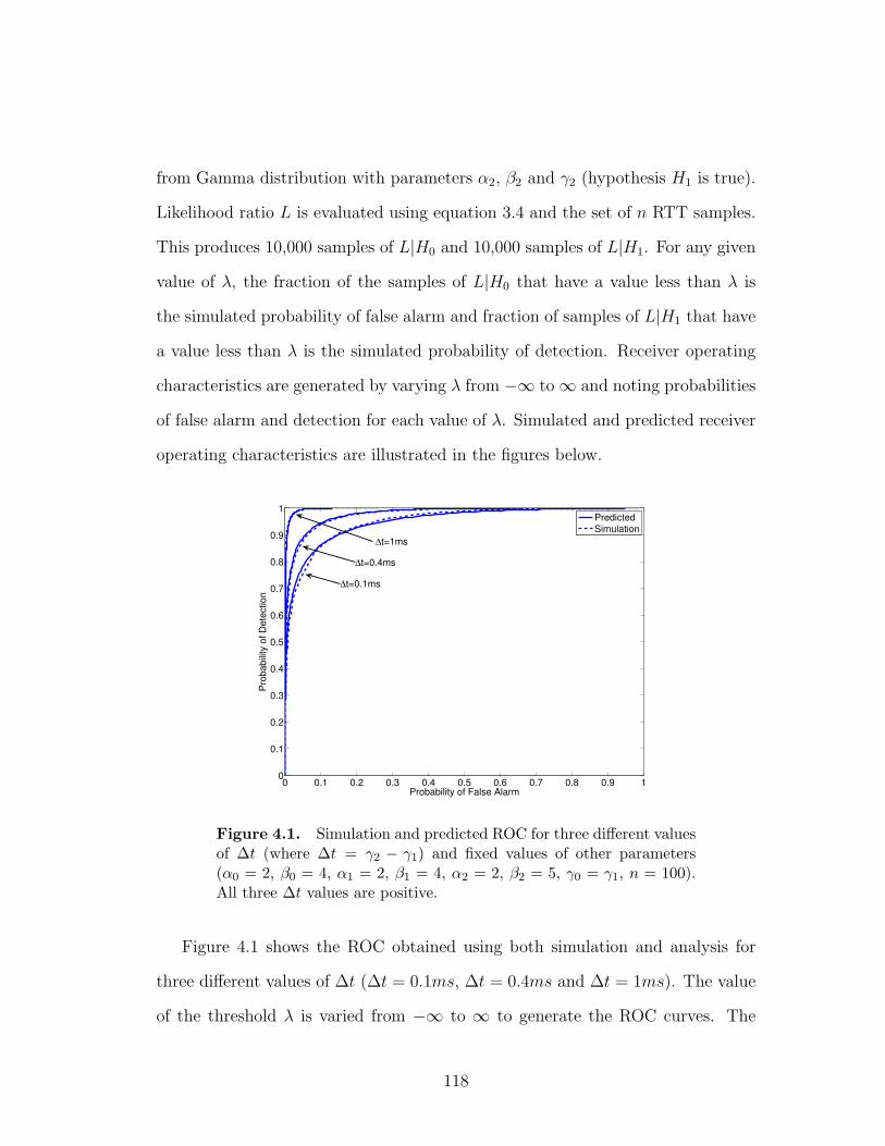
from Gamma distribution with parameters α2, β2 and γ2 (hypothesis H1 is true).

Likelihood ratio L is evaluated using equation 3.4 and the set of n RTT samples.

This produces 10,000 samples of L|H0 and 10,000 samples of L|H1. For any given

value of λ, the fraction of the samples of L|H0 that have a value less than λ is

the simulated probability of false alarm and fraction of samples of L|H1 that have

a value less than λ is the simulated probability of detection. Receiver operating

characteristics are generated by varying λ from −∞ to∞ and noting probabilities

of false alarm and detection for each value of λ. Simulated and predicted receiver

operating characteristics are illustrated in the figures below.

0 0.1 0.2 0.3 0.4 0.5 0.6 0.7 0.8 0.9 10

0.1

0.2

0.3

0.4

0.5

0.6

0.7

0.8

0.9

1

Probability of False Alarm

Prob

abilit

y of

Det

ectio

n

PredictedSimulation

∆t=0.1ms

∆t=0.4ms

∆t=1ms

Figure 4.1. Simulation and predicted ROC for three different valuesof ∆t (where ∆t = γ2 − γ1) and fixed values of other parameters(α0 = 2, β0 = 4, α1 = 2, β1 = 4, α2 = 2, β2 = 5, γ0 = γ1, n = 100).All three ∆t values are positive.

Figure 4.1 shows the ROC obtained using both simulation and analysis for

three different values of ∆t (∆t = 0.1ms, ∆t = 0.4ms and ∆t = 1ms). The value

of the threshold λ is varied from −∞ to ∞ to generate the ROC curves. The

118

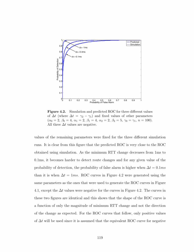
0 0.1 0.2 0.3 0.4 0.5 0.6 0.7 0.8 0.9 10

0.1

0.2

0.3

0.4

0.5

0.6

0.7

0.8

0.9

1


Prob

abilit

y of

Det

ectio

n

PredictedSimulation

∆t=−1ms

∆t=−0.4ms

∆t=−0.1ms

Figure 4.2. Simulation and predicted ROC for three different valuesof ∆t (where ∆t = γ2 − γ1) and fixed values of other parameters(α0 = 2, β0 = 4, α1 = 2, β1 = 4, α2 = 2, β2 = 5, γ0 = γ1, n = 100).All three ∆t values are negative.

values of the remaining parameters were fixed for the three different simulation

runs. It is clear from this figure that the predicted ROC is very close to the ROC

obtained using simulation. As the minimum RTT change decreases from 1ms to

0.1ms, it becomes harder to detect route changes and for any given value of the

probability of detection, the probability of false alarm is higher when ∆t = 0.1ms

than it is when ∆t = 1ms. ROC curves in Figure 4.2 were generated using the

same parameters as the ones that were used to generate the ROC curves in Figure

4.1, except the ∆t values were negative for the curves in Figure 4.2. The curves in

these two figures are identical and this shows that the shape of the ROC curve is

a function of only the magnitude of minimum RTT change and not the direction

of the change as expected. For the ROC curves that follow, only positive values

of ∆t will be used since it is assumed that the equivalent ROC curve for negative

119

value of ∆t of the same magnitude is identical as expected.

0 0.1 0.2 0.3 0.4 0.5 0.6 0.7 0.8 0.9 10

0.1

0.2

0.3

0.4

0.5

0.6

0.7

0.8

0.9

1


Prob

abilit

y of

Det

ectio

n

PredictedSimulation

n=50

n=100

n=200

Figure 4.3. Simulation and predicted ROC for three different valuesof n and fixed values of other parameters (α0 = 2, β0 = 4, α1 = 2,β1 = 4, α2 = 2, β2 = 5, γ0 = γ1, ∆t = 0.1ms)

Figure 4.3 illustrates the ROC curves for three different values of the window

size n. All other parameters are fixed including ∆t which is fixed at 0.1ms. For

each of the three different values of n, the predicted ROC curve is very close to

the ROC curve from simulation. The ROC curve for a window size of 200 samples

is to the top and left of the ROC curves for window sizes 100 and 50. For any

fixed value of probability of detection, a window size of 200 allows PAD to achieve

a lower probability of false alarm than a window size of 100 or 50 as expected.

n = 50 n = 30 n = 20PF 8.4e-28 6.2e-18 3.0e-12

Table 4.1. Value of PF for PAD with PD fixed at 0.99999 for dif-ferent values of n and fixed values of other parameters (α0 = 0.12,β0 = 1.99, α1 = 0.12, β1 = 1.99, α2 = 0.5, β2 = 3, γ0 = γ1, ∆t = 1ms)

For the ROC curves shown in figures 4.1, 4.2 and 4.3, RTT samples were

120

drawn from Gamma distribution with α = 2 and β = 4. RTTs have very high

variance for this set of parameter values and this models the RTTs of a path

with a highly loaded (congested) router output port somewhere in the path. A

majority of the Internet paths on which measurements were conducted did not

have a heavily loaded router and RTTs had a lower delay variation. Parame-

ter values of α = 0.12 and β = 1.99 were used to obtain the PF results shown

in Table 4.1. These parameters were estimated from Internet RTT measure-

ments between planck227.test.ibbt.be (Ghent University, Belgium) and planet-

lab1.larc.usp.br (University of Sao Paulo, Brazil) on October 21, 2006. Probabil-

ity of false alarm with probability of detection fixed at 0.999 are shown in Table

4.1 for three window sizes of 20, 30 and 50. Minimum RTT change was fixed at

∆t = 1ms for all three simulations. It is clear from the results in Table 4.1 that

with a suitable value of the threshold λ and with a window size as small as 20

samples, PAD can detect minimum RTT change of 1ms with a probability of de-

tection approximately 1 and probability of false alarm approximately zero. ROC

curves are a function of the parameters of Gamma distribution from which RTT

samples are drawn. This is illustrated further in Figure 4.4 where three different

ROC curves are plotted for three different values of α.

A rigorous simulation study was conducted to find the region of acceptable

performance for the parameter aware detector (PAD). If for any given threshold,

the probability of detection ≥ 0.999 and probability of false alarm ≤ 0.001, then

PAD is defined here to have acceptable performance for those parameter values.

Parameters α and β were varied from 0.5 to 5 in steps of 0.1, the parameter n was

varied from 100 to 300 in steps of 100 and the parameter ∆T was varied from 1ms

to 4ms in steps of 1ms. For each combination of the parameter values, the analysis

121

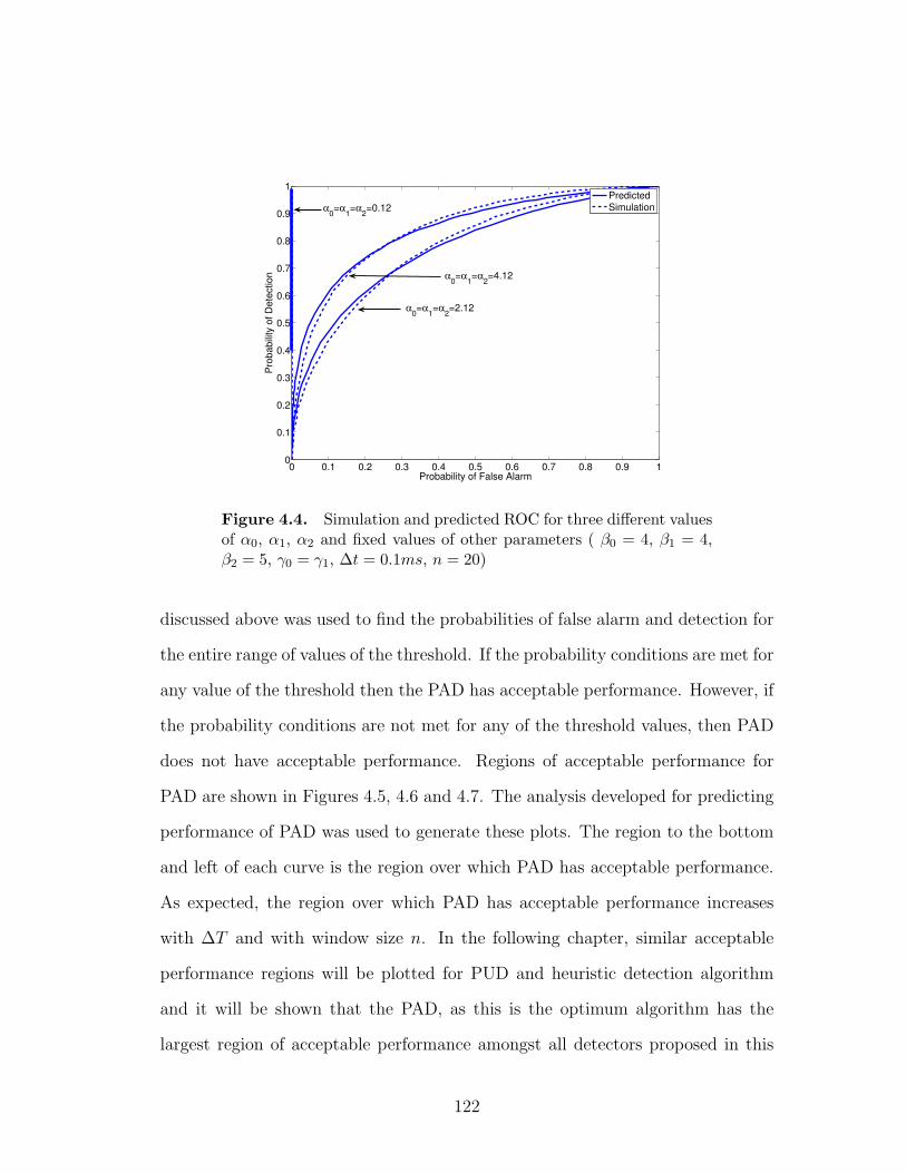
0 0.1 0.2 0.3 0.4 0.5 0.6 0.7 0.8 0.9 10

0.1

0.2

0.3

0.4

0.5

0.6

0.7

0.8

0.9

1


Prob

abilit

y of

Det

ectio

n

PredictedSimulationα0=α1=α2=0.12

α0=α1=α2=2.12

α0=α1=α2=4.12

Figure 4.4. Simulation and predicted ROC for three different valuesof α0, α1, α2 and fixed values of other parameters ( β0 = 4, β1 = 4,β2 = 5, γ0 = γ1, ∆t = 0.1ms, n = 20)

discussed above was used to find the probabilities of false alarm and detection for

the entire range of values of the threshold. If the probability conditions are met for

any value of the threshold then the PAD has acceptable performance. However, if

the probability conditions are not met for any of the threshold values, then PAD

does not have acceptable performance. Regions of acceptable performance for

PAD are shown in Figures 4.5, 4.6 and 4.7. The analysis developed for predicting

performance of PAD was used to generate these plots. The region to the bottom

and left of each curve is the region over which PAD has acceptable performance.

As expected, the region over which PAD has acceptable performance increases

with ∆T and with window size n. In the following chapter, similar acceptable

performance regions will be plotted for PUD and heuristic detection algorithm

and it will be shown that the PAD, as this is the optimum algorithm has the

largest region of acceptable performance amongst all detectors proposed in this

122

dissertation as expected. Note that for the plots in Figures 4.5, 4.6 and 4.7,

β2 = β + 0.5. Figure 4.8 shows how the acceptable performance region curves

change as a function of the parameter β2.

1 1.5 2 2.5 3 3.5 4 4.5 51

1.5

2

2.5

3

3.5

4

4.5

5

α

β

∆T=2ms

∆T=1ms

∆T=3ms∆T=4ms

Figure 4.5. Region of acceptable performance for parameter awaredetector with window size of 100 and α0 = α1 = α2 = α and β0 =β1 = β and β2 = β + 0.5

4.4 Summary

Given the set of parameters α0, β0, γ0, α1, β1, γ1, α2, β2, γ2, n and λ, expres-

sions for probability of detection and false alarms (Equations 4.1 and 4.2) that

were derived in this chapter, can be used to predict these probabilities for the

ideal detector. Predicted values of the probabilities of false alarm and detection

were validated using simulation in section 4.3. ROCs were plotted for sevaral

different values of the parameters ∆t, n, α and β. The ROC curve obtained using

analysis was close to the ROC curve obtained from simulation for each of the

various different combinations of the parameter values. This validates not only

123

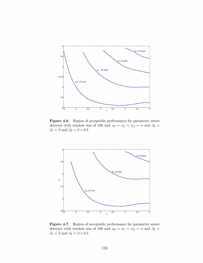
1.5 2 2.5 3 3.5 4 4.5 52

2.5

3

3.5

4

4.5

5

α

β

∆T=2ms

∆T=1ms

∆T=3ms

∆T=4ms


1.5 2 2.5 3 3.5 4 4.5 52.5

3

3.5

4

4.5

5

α

β

∆T=2ms

∆T=1ms

∆T=3ms


124

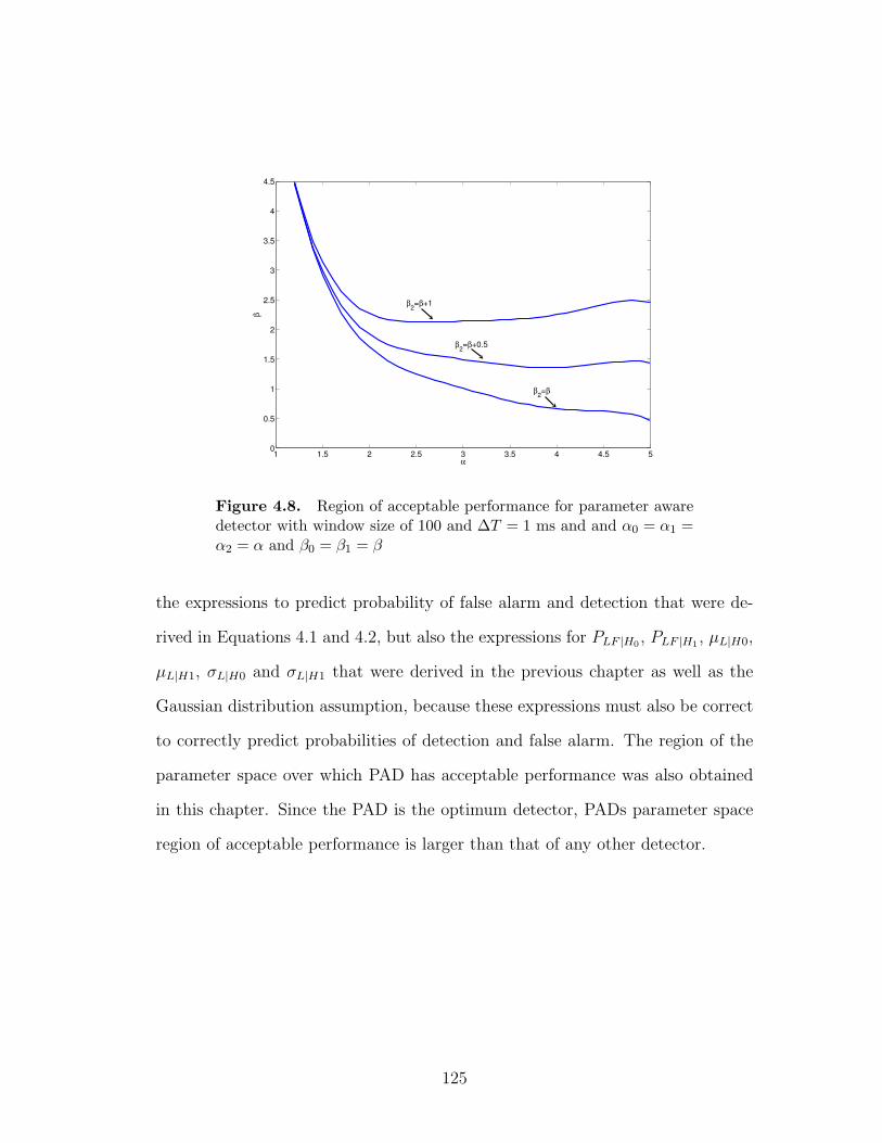
1 1.5 2 2.5 3 3.5 4 4.5 50

0.5

1

1.5

2

2.5

3

3.5

4

4.5

α

β

β2=β+1

β2=β+0.5

β2=β

Figure 4.8. Region of acceptable performance for parameter awaredetector with window size of 100 and ∆T = 1 ms and and α0 = α1 =α2 = α and β0 = β1 = β

the expressions to predict probability of false alarm and detection that were de-

rived in Equations 4.1 and 4.2, but also the expressions for PLF |H0 , PLF |H1 , µL|H0,

µL|H1, σL|H0 and σL|H1 that were derived in the previous chapter as well as the

Gaussian distribution assumption, because these expressions must also be correct

to correctly predict probabilities of detection and false alarm. The region of the

parameter space over which PAD has acceptable performance was also obtained

in this chapter. Since the PAD is the optimum detector, PADs parameter space

region of acceptable performance is larger than that of any other detector.

125

Chapter 5

Parameter Unaware Detector

5.1 Introduction

Expressions for the first two moments of L|H0 and L|H1 for the PAD were

derived in Chapter 3. These expressions were used in Chapter 4 together with a

distribution assumption to find expression for probabilities of detection and false

alarms for PAD. The predicted probabilities were then compared to the ones ob-

tained from simulation and it was found that the analysis correctly predicts these

probabilities. In the current chapter, simulation will be used to generate ROC

curves for the PUD. The performance of PUD will be compared with the perfor-

mance of the ideal detector (PAD). Simulations were also conducted to find the

region of the parameter space over which PUD and the heuristic detectors have

acceptable performance. It is shown in this chapter that PAD has the largest re-

gion of acceptable performance followed by PUD and then by the heuristics-based

algorithm. PUD is also applied to the measured data to evaluate its performance.

126

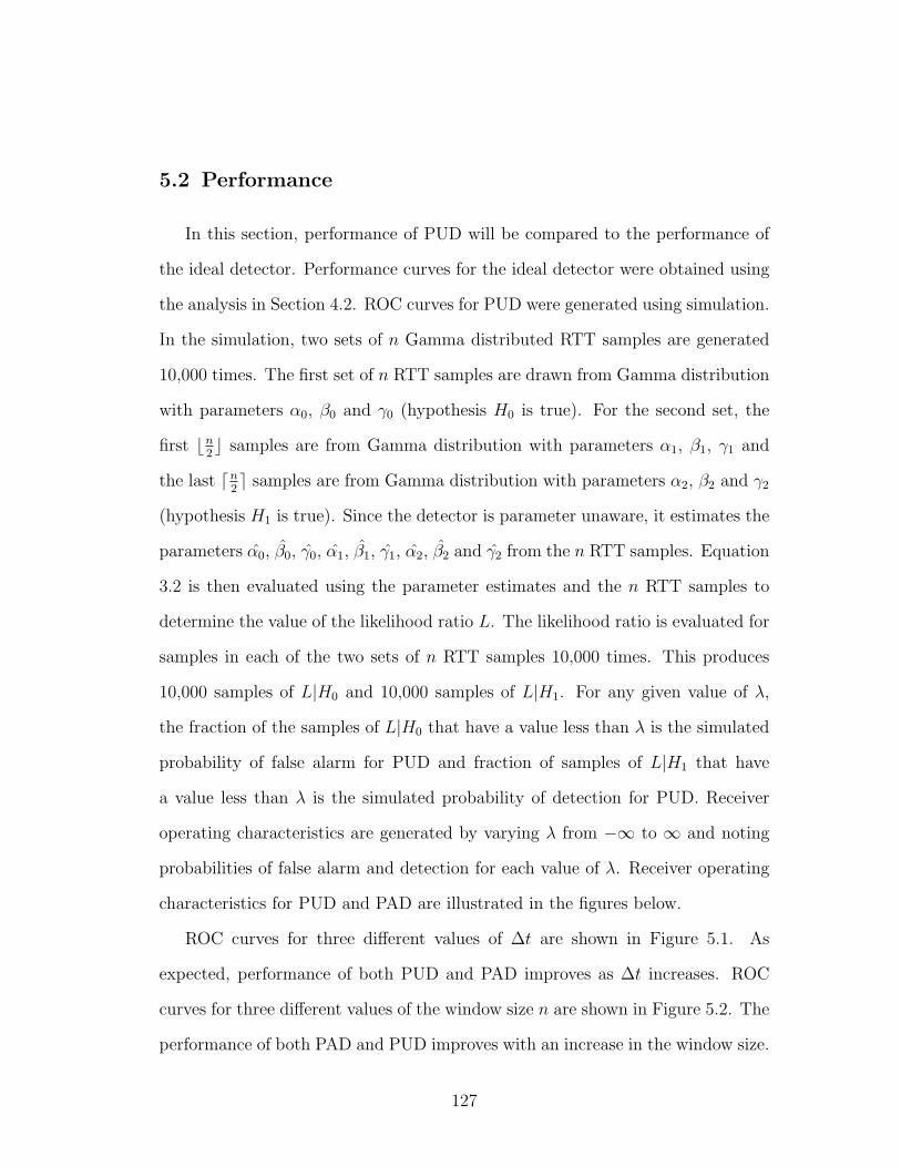
5.2 Performance

In this section, performance of PUD will be compared to the performance of

the ideal detector. Performance curves for the ideal detector were obtained using

the analysis in Section 4.2. ROC curves for PUD were generated using simulation.

In the simulation, two sets of n Gamma distributed RTT samples are generated

10,000 times. The first set of n RTT samples are drawn from Gamma distribution

with parameters α0, β0 and γ0 (hypothesis H0 is true). For the second set, the

first bn2c samples are from Gamma distribution with parameters α1, β1, γ1 and

the last dn2e samples are from Gamma distribution with parameters α2, β2 and γ2

(hypothesis H1 is true). Since the detector is parameter unaware, it estimates the

parameters α̂0, β̂0, γ̂0, α̂1, β̂1, γ̂1, α̂2, β̂2 and γ̂2 from the n RTT samples. Equation

3.2 is then evaluated using the parameter estimates and the n RTT samples to

determine the value of the likelihood ratio L. The likelihood ratio is evaluated for

samples in each of the two sets of n RTT samples 10,000 times. This produces

10,000 samples of L|H0 and 10,000 samples of L|H1. For any given value of λ,

the fraction of the samples of L|H0 that have a value less than λ is the simulated

probability of false alarm for PUD and fraction of samples of L|H1 that have

a value less than λ is the simulated probability of detection for PUD. Receiver

operating characteristics are generated by varying λ from −∞ to ∞ and noting

probabilities of false alarm and detection for each value of λ. Receiver operating

characteristics for PUD and PAD are illustrated in the figures below.

ROC curves for three different values of ∆t are shown in Figure 5.1. As

expected, performance of both PUD and PAD improves as ∆t increases. ROC

curves for three different values of the window size n are shown in Figure 5.2. The

performance of both PAD and PUD improves with an increase in the window size.

127

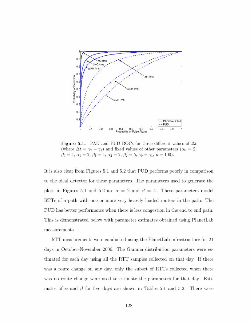
0 0.1 0.2 0.3 0.4 0.5 0.6 0.7 0.8 0.9 10

0.1

0.2

0.3

0.4

0.5

0.6

0.7

0.8

0.9

1


Prob

abilit

y of

Det

ectio

n

PAD PredictedPUD

∆t=1ms∆t=0.4ms

∆t=0.1ms

∆t=0.1ms

∆t=0.4ms

∆t=1ms

Figure 5.1. PAD and PUD ROCs for three different values of ∆t(where ∆t = γ2 − γ1) and fixed values of other parameters (α0 = 2,β0 = 4, α1 = 2, β1 = 4, α2 = 2, β2 = 5, γ0 = γ1, n = 100).

It is also clear from Figures 5.1 and 5.2 that PUD performs poorly in comparison

to the ideal detector for these parameters. The parameters used to generate the

plots in Figures 5.1 and 5.2 are α = 2 and β = 4. These parameters model

RTTs of a path with one or more very heavily loaded routers in the path. The

PUD has better performance when there is less congestion in the end to end path.

This is demonstrated below with parameter estimates obtained using PlanetLab

measurements.

RTT measurements were conducted using the PlanetLab infrastructure for 21

days in October-November 2006. The Gamma distribution parameters were es-

timated for each day using all the RTT samples collected on that day. If there

was a route change on any day, only the subset of RTTs collected when there

was no route change were used to estimate the parameters for that day. Esti-

mates of α and β for five days are shown in Tables 5.1 and 5.2. There were

128

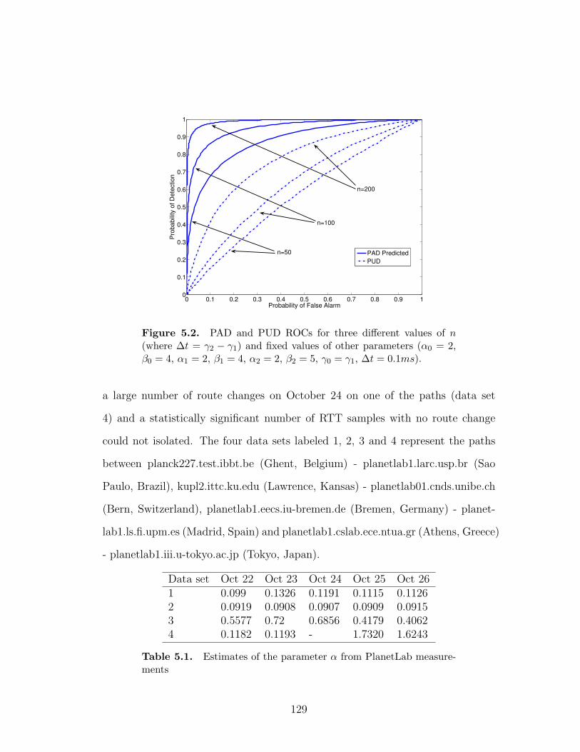
0 0.1 0.2 0.3 0.4 0.5 0.6 0.7 0.8 0.9 10

0.1

0.2

0.3

0.4

0.5

0.6

0.7

0.8

0.9

1


Prob

abilit

y of

Det

ectio

n

PAD PredictedPUD

n=50

n=100

n=200

Figure 5.2. PAD and PUD ROCs for three different values of n(where ∆t = γ2 − γ1) and fixed values of other parameters (α0 = 2,β0 = 4, α1 = 2, β1 = 4, α2 = 2, β2 = 5, γ0 = γ1, ∆t = 0.1ms).

a large number of route changes on October 24 on one of the paths (data set

4) and a statistically significant number of RTT samples with no route change

could not isolated. The four data sets labeled 1, 2, 3 and 4 represent the paths

between planck227.test.ibbt.be (Ghent, Belgium) - planetlab1.larc.usp.br (Sao

Paulo, Brazil), kupl2.ittc.ku.edu (Lawrence, Kansas) - planetlab01.cnds.unibe.ch

(Bern, Switzerland), planetlab1.eecs.iu-bremen.de (Bremen, Germany) - planet-

lab1.ls.fi.upm.es (Madrid, Spain) and planetlab1.cslab.ece.ntua.gr (Athens, Greece)

- planetlab1.iii.u-tokyo.ac.jp (Tokyo, Japan).

Data set Oct 22 Oct 23 Oct 24 Oct 25 Oct 261 0.099 0.1326 0.1191 0.1115 0.11262 0.0919 0.0908 0.0907 0.0909 0.09153 0.5577 0.72 0.6856 0.4179 0.40624 0.1182 0.1193 - 1.7320 1.6243

Table 5.1. Estimates of the parameter α from PlanetLab measure-ments

129

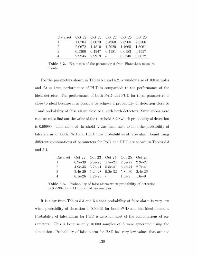
Data set Oct 22 Oct 23 Oct 24 Oct 25 Oct 261 1.0704 3.6073 3.4260 2.6908 2.67062 2.0672 1.4810 1.5020 1.4665 1.30613 0.5306 0.4547 0.4181 0.6183 0.75574 2.9245 2.9919 - 0.5748 0.6072

Table 5.2. Estimates of the parameter β from PlanetLab measure-ments

For the parameters shown in Tables 5.1 and 5.2, a window size of 100 samples

and ∆t = 1ms, performance of PUD is comparable to the performance of the

ideal detector. The performance of both PAD and PUD for these parameters is

close to ideal because it is possible to achieve a probability of detection close to

1 and probability of false alarm close to 0 with both detectors. Simulations were

conducted to find out the value of the threshold λ for which probability of detection

is 0.99999. This value of threshold λ was then used to find the probability of

false alarm for both PAD and PUD. The probabilities of false alarm found using

different combinations of parameters for PAD and PUD are shown in Tables 5.3

and 5.4.

Data set Oct 22 Oct 23 Oct 24 Oct 25 Oct 261 6.9e-39 5.6e-23 1.5e-24 2.6e-27 2.9e-272 4.9e-35 5.7e-41 5.5e-41 6.4e-41 2.7e-413 3.4e-29 1.2e-28 9.2e-32 5.8e-30 2.4e-264 6.1e-26 1.2e-25 - 1.3e-9 1.6e-9

Table 5.3. Probability of false alarm when probability of detectionis 0.99999 for PAD obtained via analysis

It is clear from Tables 5.3 and 5.4 that probability of false alarm is very low

when probability of detection is 0.99999 for both PUD and the ideal detector.

Probability of false alarm for PUD is zero for most of the combinations of pa-

rameters. This is because only 10,000 samples of L were generated using the

simulation. Probability of false alarm for PAD has very low values that are not

130

Data set Oct 22 Oct 23 Oct 24 Oct 25 Oct 261 0 0 0 0 02 0 0 0 0 03 0 0 0 0 04 0 0 - 0.0092 0.0029

Table 5.4. Probability of false alarm when probability of detectionis 0.99999 for PUD obtained using simulations

zero because these probability values were generated using the analysis.

5.3 Acceptable performance regions

Extensive simulations were conducted to find the range of parameter values for

which PUD has acceptable performance. Acceptable performance is defined to be

achieved by a detector when PD ≥ 0.999, PF ≤ 0.001. Parameters α and β were

varied from 0.1 to 4 and from 0.1 to 3 respectively in steps of 0.1, parameter n

was varied from 100 to 300 in steps of 100 samples and parameter ∆T was varied

from 1ms to 4ms in steps of 1ms. For each combination of the values of α, β, n

and ∆T , 10,000 samples of L|H0 and 10,000 samples of L|H1 were generated. The

RTT samples needed to find L|H0 and L|H1 were samples drawn from a Gamma

distribution. Threshold λ was then varied from −∞ to ∞ to determine if PUD

has acceptable performance for any value of threshold for the given parameters.

Here the detection algorithm is defined to have acceptable performance when

probability of detection is greater than 0.999 and probability of false alarm is less

than 0.001. Simulation results with n fixed at 100 samples are shown in Figure

5.3. Parameter space for which PUD has acceptable performance is to the bottom

and left of each curve. For example, when α = 3 and β = 2, route changes with a

minimum RTT change of 4ms can be detected with PD ≥ 0.999 and PF ≤ 0.001

using PUD, however if minimum RTT changes by 3, 2 or 1ms, PUD cannot detect

131

these changes with acceptable performance. Note that the curves shown in Figure

5.3 were fitted from the data using a polynomial of degree 4. Simulation results

that depict the parameter space over which PUD has acceptable performance

when n = 200 and n = 300 are shown in Figures 5.4 and 5.5. As expected,

parameter space over which PUD has acceptable performance increases with an

increase in n.

0.5 1 1.5 2 2.5 3 3.5 40

0.5

1

1.5

2

2.5

3

α

β

∆T=1ms∆T=2ms

∆T=3ms

∆T=4ms

Figure 5.3. Parameter space for which PUD has acceptable perfor-mance (PD ≥ 0.999, PF ≤ 0.001) is to the bottom and left of eachcurve. Window size n is fixed at 100 samples and α0 = α1 = α2 = α,β0 = β1 = β, β2 = β + 0.5.

Similar simulations were conducted to find the range of parameter values for

which the heuristic route change detection algorithm has acceptable performance.

Parameters α and β were varied from 0.5 to 5 and 0.5 to 3 in steps of 0.1 respec-

tively and the window size n was varied from 100 samples to 300 samples in steps

of 100 samples. The parameter ∆T was fixed at 1ms and the simulations were

not repeated for different values of ∆T because it is expected that the parameter

132

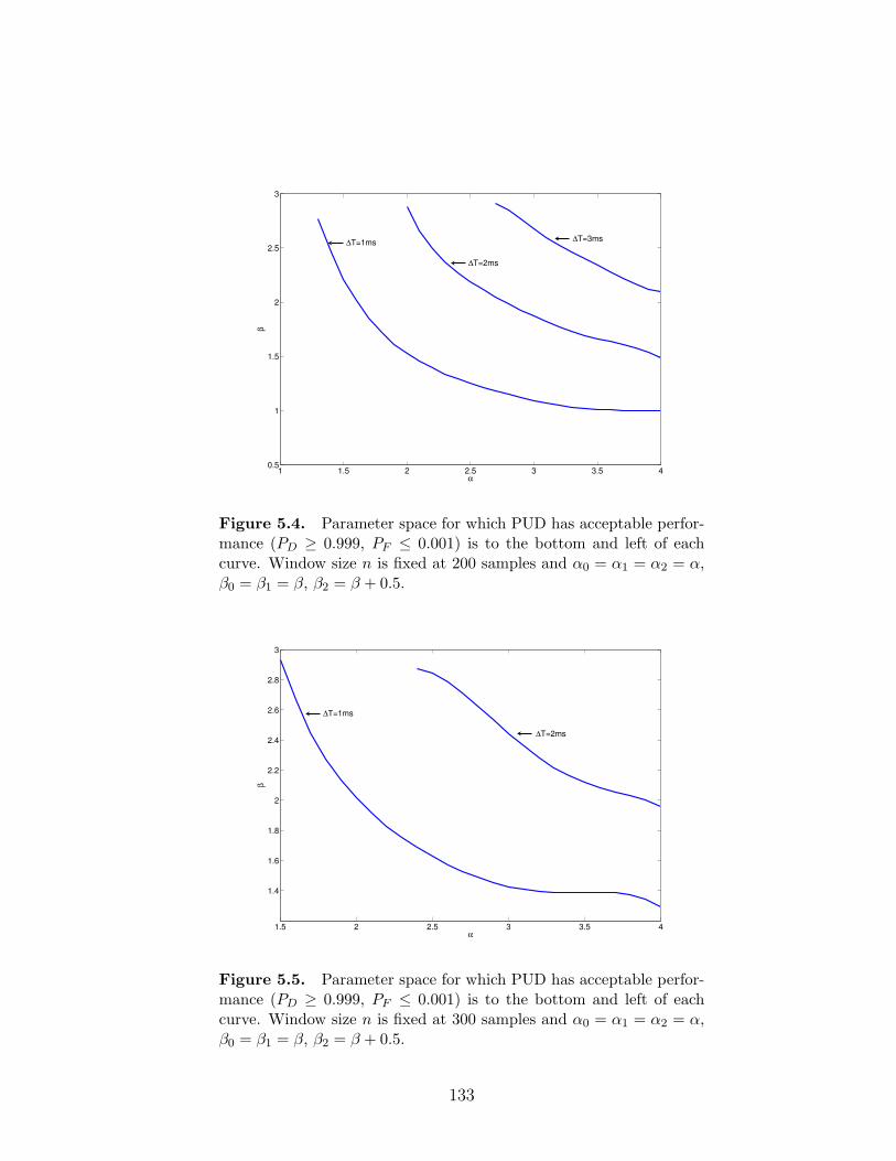
1 1.5 2 2.5 3 3.5 40.5

1

1.5

2

2.5

3

α

β

∆T=1ms

∆T=2ms

∆T=3ms


1.5 2 2.5 3 3.5 4

1.4

1.6

1.8

2

2.2

2.4

2.6

2.8

3

α

β

∆T=1ms

∆T=2ms


133

space is not a function of the parameter ∆T (the heuristic algorithm just looks

at the past few windows of samples to decide whether or not it can detect route

changes and if the congestion is high, it does not even attempt to detect the route

change). For each combination of the parameter values, two traces are generated,

one that has 10,000 route changes and another that has no route changes. The

heuristic algorithm is then applied to these traces to find out the probabilities of

detection and false alarm. If the probability of detection is greater than 0.999 and

probability of false alarm less than 0.001, then the heuristic algorithm has accept-

able performance for that set of parameter values. Figure 5.6 shows the range

of parameter values for which the heuristic algorithm has acceptable performance

for three different window size values.

0.8 1 1.2 1.4 1.6 1.8 2 2.20.4

0.6

0.8

1

1.2

1.4

1.6

1.8

2

α

β

Window Size=100Window Size=200Window Size=300

Figure 5.6. Parameter space for which the heuristic algorithm hasacceptable performance (PD ≥ 0.999, PF ≤ 0.001) is to the bottomand left of each curve. Parameter ∆T is fixed at 1ms.

Parameter spaces of all three algorithms for window size of 100 samples and

∆T=1ms are shown in the same graph in Figure 5.7. As expected, PAD has the

134

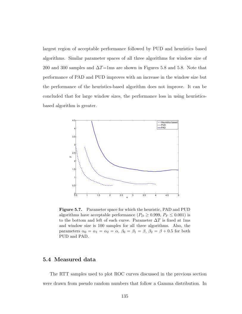
largest region of acceptable performance followed by PUD and heuristics based

algorithms. Similar parameter spaces of all three algorithms for window size of

200 and 300 samples and ∆T=1ms are shown in Figures 5.8 and 5.8. Note that

performance of PAD and PUD improves with an increase in the window size but

the performance of the heuristics-based algorithm does not improve. It can be

concluded that for large window sizes, the performance loss in using heuristics-

based algorithm is greater.

0.5 1 1.5 2 2.5 3 3.5 4 4.5 50

0.5

1

1.5

2

2.5

3

3.5

4

4.5

α

β

Heuristics basedPUDPAD

Figure 5.7. Parameter space for which the heuristic, PAD and PUDalgorithms have acceptable performance (PD ≥ 0.999, PF ≤ 0.001) isto the bottom and left of each curve. Parameter ∆T is fixed at 1msand window size is 100 samples for all three algorithms. Also, theparameters α0 = α1 = α2 = α, β0 = β1 = β, β2 = β + 0.5 for bothPUD and PAD.

5.4 Measured data

The RTT samples used to plot ROC curves discussed in the previous section

were drawn from pseudo random numbers that follow a Gamma distribution. In

135

0.5 1 1.5 2 2.5 3 3.5 4 4.5 50

0.5

1

1.5

2

2.5

3

3.5

4

4.5

5

α

β



this section, these performance curves are plotted using RTT samples that were

collected using the PlanetLab infrastructure. To plot the ROC curves for measured

RTT data, the data was first segmented into statistically homogeneous regions

with no route changes. The minimum RTT of these samples was then subtracted

from all the RTT samples to change the minimum to zero. These RTT samples

were then divided into windows of size n samples each. The likelihood ratio was

then calculated for each of these n sample windows. This produces samples for L

when hypothesis H0 is true. The minimum RTT of the last dn2e samples was then

changed by adding ∆t for each of the n sample windows. Likelihood ratio was

then calculated again for each of these n RTT sample windows. This produces

samples for L when hypothesis H1 is true. For any given value of threshold λ, the

136

0.5 1 1.5 2 2.5 3 3.5 4 4.5 50

0.5

1

1.5

2

2.5

3

3.5

4

α

β



fraction of the samples of L|H0 that have a value less than λ is the probability of

false alarm for PUD and fraction of samples of L|H1 that have a value less than

λ is the probability of detection for PUD. Receiver operating characteristics are

generated by varying λ from −∞ to ∞ and noting probabilities of false alarm

and detection for each value of λ. The ROC curves in Figures 5.10 and 5.11

were plotted using RTT samples collected on October 23, 2006. As expected,

performance of PUD improves with an increase in the window size and minimum

RTT change ∆T . The ROC curve shown in Figure 5.12 was plotted using RTT

samples collected on October 25, 2006. A window size of 100 samples is sufficient

to detect route changes with a high value of probability of detection and small

probability of false alarm on this day.

137

0 0.1 0.2 0.3 0.4 0.5 0.6 0.7 0.8 0.9 10

0.1

0.2

0.3

0.4

0.5

0.6

0.7

0.8

0.9

1


Prob

abilit

y of

Det

ectio

n

n=100n=50n=30

Figure 5.10. PUD ROCs for three different values of n and ∆t fixedat 1ms. RTT samples are from data set 4 collected on October 23, 2006

0 0.02 0.04 0.06 0.08 0.1 0.12 0.14 0.160.3

0.4

0.5

0.6

0.7

0.8

0.9

1


Prob

abilit

y of

Det

ectio

n

∆ T=1ms∆ T=2ms∆ T=3ms

Figure 5.11. PUD ROCs for three different values of ∆t and withn fixed at 100 samples. RTT samples are from data set 4 collected onOctober 23, 2006

138

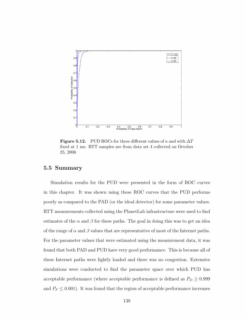
0 0.1 0.2 0.3 0.4 0.5 0.6 0.7 0.8 0.9 10

0.1

0.2

0.3

0.4

0.5

0.6

0.7

0.8

0.9

1


Prob

abilit

y of

Det

ectio

n

n=100n=50n=30

Figure 5.12. PUD ROCs for three different values of n and with ∆Tfixed at 1 ms. RTT samples are from data set 4 collected on October25, 2006

5.5 Summary

Simulation results for the PUD were presented in the form of ROC curves

in this chapter. It was shown using these ROC curves that the PUD performs

poorly as compared to the PAD (or the ideal detector) for some parameter values.

RTT measurements collected using the PlanetLab infrastructure were used to find

estimates of the α and β for these paths. The goal in doing this was to get an idea

of the range of α and β values that are representative of most of the Internet paths.

For the parameter values that were estimated using the measurement data, it was

found that both PAD and PUD have very good performance. This is because all of

these Internet paths were lightly loaded and there was no congestion. Extensive

simulations were conducted to find the parameter space over which PUD has

acceptable performance (where acceptable performance is defined as PD ≥ 0.999

and PF ≤ 0.001). It was found that the region of acceptable performance increases

139

with an increase in ∆T or the window size as expected. Acceptable performance

region for the heuristic detector was also obtained in this chapter. It was shown

that the PAD has the largest region of acceptable performance followed by PUD

and then by the heuristics-based detector. This is an important result because it

shows that PUD is the practical detector of choice because it has a larger region

of acceptable performance than the heuristics-based algorithm. PUD can detect

route change events with better accuracy than the heuristics-based detector when

the router queues are heavily loaded. Moreover it was shown that the difference in

performance of heuristics-based algorithm and the PUD increases with an increase

in the window size. Finally, PUD was applied to Internet measurement traces in

which multiple route changes were induced to evaluate its performance.

The acceptable performance region curves shown in Figures 5.7, 5.8 and 5.9

are very useful for determining the detection algorithm to use and the minimum

required probing rate given some performance constraints. For example, consider

the case where route changes that occur 1 minute apart in time are to be detected

and assume that from historical data it is known that the path gets congesting

raising the α and β values to 3 and 1.4 respectively. From the three figures it is

clear that only PUD can detect route changes with acceptable performance and

only when window size is 300 samples. Since route changes that occur 1 minute

apart in time are to be detected, the maximum inter-sample time is 200ms. Also,

it is clear from these figures that the heuristic algorithm does not have acceptable

performance even when the probing rate is 5 samples per second. If it is known

from historical data that there is no congestion in this path, a lower sampling

rate of 100 samples per second can be used. This procedure of determining the

minimum sampling rate can be automated and implemented in the detector. A

140

detector can use the last few samples to estimate the α and β parameter values

and then use the information in Figures 5.7, 5.8 and 5.9 to determine the min-

imum required window size and the minimum sampling rate. The detector can

then adjust its sampling rate accordingly in real-time so as to achieve acceptable

performance.

This chapter concludes the series of chapters on route change detectors. In

the next chapter, it will be shown that the PF scheduler used in wireless networks

can cause RTM impairments. A new scheduler that mitigates the starvation

vulnerability of the proportional fair scheduler is also developed and evaluated in

the next chapter.

141

Chapter 6

Scheduler-Induced Imparments in

Infrastructure-Based Wireless

Networks

6.1 Introduction

Methods for detecting RTM application impairments were introduced in Chap-

ter 2. Impairments may occur during congestion or route change events. Methods

for detecting congestion and route change events were also developed in Chapters

2, 3, 4 and 5. Measured RTTs are used together with packet loss information to

detect congestion and route changes. These detection methods are based on cer-

tain assumptions about the random variable that models the RTTs (e.g., RTTs are

Gamma distributed). These assumptions about the RTT may not hold when there

are one or more wireless links in the end-to-end path. Wireless links are typically

characterized by link rate variations (due to mobility, fading, etc.), high error rates

and very high available bandwidth variations. For these reasons, the wireless links

142

typically exhibit very high delay variations. A study of infrastructure-based wire-

less networks was initiated to better understand the delay characteristics of these

networks. During this study, it was found that the proportional fair scheduler that

is commonly used in these networks induces RTM application impairments. As a

part of this work, these impairments were identified using field experiments. More

importantly, new mechanisms were developed to illustrate these performance is-

sues. The contribution of this work is the finding that impairments are induced

by the proportional fair scheduler and also the development and analysis of a new

scheduler to improve the performance.

Many infrastructure-based wireless networks (e.g., Evolution-Data Optimized

(EVDO) [XY06] and High-Speed Downlink Packet Access (HSDPA)) use the

proportional-fair scheduling algorithm. This algorithm is designed to achieve good

network throughput by scheduling users that are experiencing their better-than-

average channel conditions without compromising long-term fairness. It will be

shown in this chapter using field data that this fairness-ensuring mechanism can be

easily corrupted, accidentally or deliberately, to starve users and severely degrade

performance reducing TCP throughput and thus inducing RTM impairments. The

performance degradation is quantified using results from experiments that were

conducted in both in-lab and with a production CDMA 1xEVDO network. It is

shown that delay jitter can be increased by up to 1 second and TCP throughput

can be reduced by as much as 25 − 30% by a single malicious user. A modifica-

tion to the proportional fair scheduling algorithm that mitigates this starvation

problem is also proposed and analysed in this chapter. Using ns-2 simulations, it

is shown this modification to the proportional fair scheduling algorithm mitigates

starvation without compromising the fairness ensuring and throughput optimizing

143

mechanisms of the base algorithm.

6.2 The PF algorithm and starvation

As with any managed wireless network, access to the wireless channel in 3G

networks is controlled by Base Stations (BSs) to which mobile devices or Access

Terminals (ATs) are associated. The focus here is on Proportional Fair (PF) -

the scheduling algorithm [VTL02] used to schedule transmissions on the downlink

in most 3G networks. In these networks, downlink transmission is slotted. For

example, in CDMA-based EV-DO networks, slot size is 1.67ms. BSs have per-AT

queues and employ PF to determine the AT to transmit to in a specific time slot.

The inputs to PF are the current channel conditions reported on a per-slot

basis by each AT. Specifically, each AT uses its current Signal-to-Noise Ratio

(SNR) to determine the required coding rate and modulation type and hence,

the achievable rate of downlink transmission. In the EV-DO system, there are

10 unique achievable data rates (in Kilobits per second) - 0, 38.4, 76.8, 153.6,

307.2, 614.4, 921.6, 1228.8, 1843.2 and 2457.6. Assume that there are n ATs in

the system. Denote the achievable data rate reported by AT i in time slot t to be

Rit (i = 1 . . . n). For each AT i, the scheduler also maintains Ait, an exponentially-

weighted average rate that user i has achieved, i.e.,

Ait =

Ait−1(1− α) + αRit if slot allocated

Ait−1(1− α) otherwise

Slot t is allocated to the AT with the highest ratioRitAit−1

. Parameter α has a value

that is usually around 0.001 [JPP00]. Thus, an AT will be scheduled less often

144

when it experiences fading and more often when it does not.

The basic observation behind this work is that an AT can (deliberately or

accidentally) influence the value of its RtAt−1

ratio thereby affecting the slot alloca-

tion process. An AT can do this simply by receiving data in an on-off manner.

To see why, consider an AT that receives no data for several slots. Its At would

slowly reduce and approach zero. After several inactive slots, when a new packet

destined for that AT arrives at the base station, that AT has a low value of At

and is likely to get allocated the slot because its ratio is very high. This AT keeps

getting allocated slots until its At increases enough. During this period, all other

ATs are starved. Starvation due to on-off behavior occurs because PF reduces At

during the off periods. This implies that PF “compensates” for slots that are not

allocated even when an AT has no data to receive!

6.3 Experiment configuration

The initial experiments were conducted using a production EV-DO network

in USA. The ATs are IBM T42 Thinkpad laptops running Windows XP equipped

with commercially-available PCMCIA EV-DO cards. The laptops have 2GHz

processors and 1GB of main memory. All ATs connect to the same base station

and sector. Data to the ATs is sourced from Linux PCs with 2.4GHz processors

and 1GB of memory. All of these PCs are on the same subnet and 10 or 11 hops

away from the ATs.

Two ATs - AT1 and AT2 were used for the first experiment. AT1 receives

a long-lived periodic UDP packet stream consisting of 1500-byte packets with

an average rate of 600Kbps. AT2 is assigned the role of a malicious AT and

hence, receives traffic in an on-off pattern from its sender. Specifically, it receives

145

0 10 20 30 40 50 60 700

0.2

0.4

0.6

0.8

1

1.2

Time [sec]

Exce

ss O

ne−w

ay D

elay

[sec

]

Figure 6.1. “Jitter” caused by a malicious AT in a commercial EV-DO network.

a burst of 250 packets of 1500 bytes every 6 seconds. The “jitter” experienced

by AT1 is shown in Figure 6.1. Since the ATs are not time-synchronized with

the senders, jitter is calculated as the excess one-way delays over the minimum

delay. Well-defined increases in jitter are observed whenever a burst is sent to AT2.

These results clearly show that AT1 experiences extraordinary increase in “jitter”.

Similar results are observed with other parameter settings (results not shown

here). With all of the parameter settings, however, the jitter increases vary from

300ms to 1 second. The variability is likely due to traffic to other ATs and queueing

effects at other hops. Hence, to understand and quantify the attack scenarios

better, a more controlled laboratory was used because it eliminates unknowns

such as cross-traffic.

The laboratory configuration includes the Base Station, the Radio Network

Controller (RNC) and the Packet Data Serving Node (PDSN) (see [JPP00]). The

links between the Base Station, RNC and PDSN are 1Gbps Ethernet links. The

146

Base Station serves 3 sectors of which only one is used for this study. The ATs

and senders are the same as before. Tcpdump [tcp] traces are collected at the

senders and ATs. Due to the peculiarities of PPP implementation on Windows

XP, the timestamps of received packets are accurate only to 16ms. However, these

inaccuracies are small enough to not affect the results. For TCP-based experi-

ments, tcptrace and tcpdump are used to analyze the sender-side traces. There are

three main differences with a commercial network. First, laboratory base stations

use lower power levels than commercial networks due to shorter distances and in

the interest of our long-term health. Since the goal is not to characterize fading

and PF’s vulnerability does not depend on channel characteristics, this does not

affect the validity of the results. Second, the number of ATs connected to the

base station can be controlled in the laboratory. Third, the number of hops from

the senders to the ATs is only 3. This eliminates the additional hops on normal

Internet paths and queueing effects on those hops. The impact of this is discussed

in Section 6.4.2. Moreover, this is realistic in networks that use split-TCP or

TCP-proxy [WZZ+06].

The laboratory configuration poses a few challenges. First, even though the

experiments were conducted in the laboratory, the wireless conditions varied signif-

icantly. Hence, up to 30 runs of each experiment (a particular parameter setting)

were conducted to calculate a good estimate of the required performance met-

ric with a small enough confidence interval. The runs of the different parameter

settings used to plot a figure were also interleaved so that they all experienced

the same wireless conditions on average. A second challenge is that ATs become

disassociated with the base station after around 12 seconds of inactivity. Also, the

initial few packets sent to an inactive AT encountered large delays due to channel

147

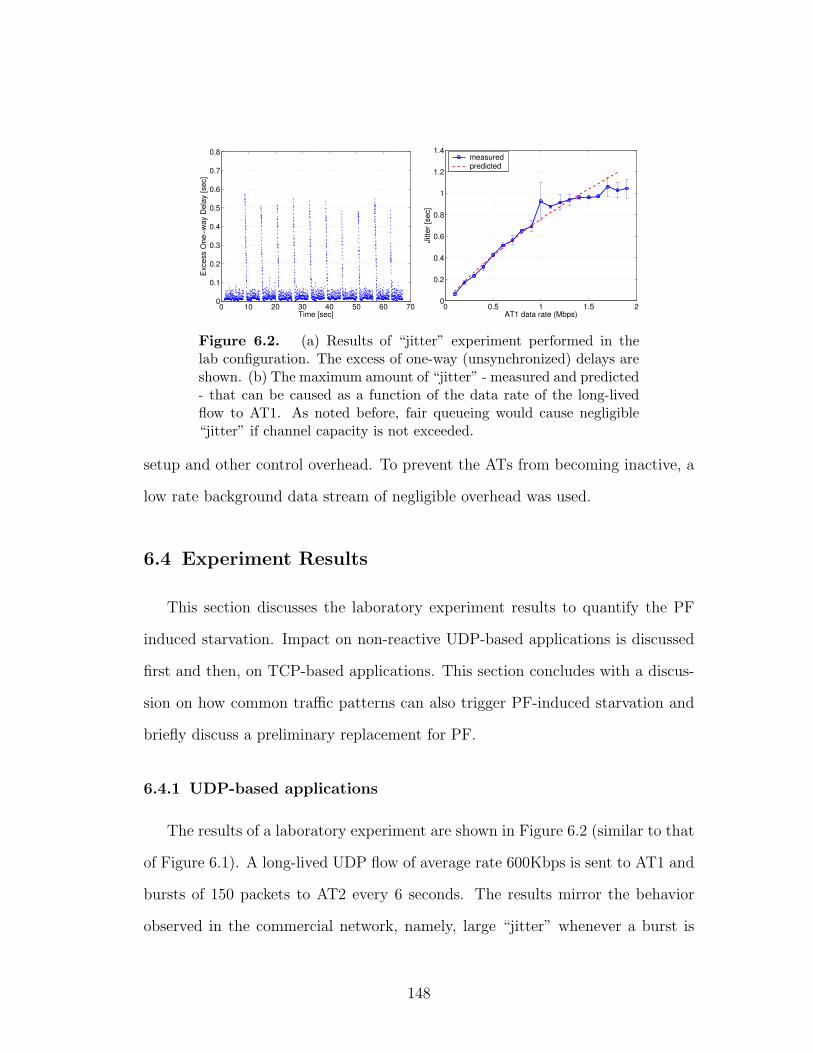
0 10 20 30 40 50 60 700

0.1

0.2

0.3

0.4

0.5

0.6

0.7

0.8

Time [sec]

Exce

ss O

ne−w

ay D

elay

[sec

]

0 0.5 1 1.5 20

0.2

0.4

0.6

0.8

1

1.2

1.4

AT1 data rate (Mbps)

Jitte

r [se

c]

measuredpredicted

Figure 6.2. (a) Results of “jitter” experiment performed in thelab configuration. The excess of one-way (unsynchronized) delays areshown. (b) The maximum amount of “jitter” - measured and predicted- that can be caused as a function of the data rate of the long-livedflow to AT1. As noted before, fair queueing would cause negligible“jitter” if channel capacity is not exceeded.

setup and other control overhead. To prevent the ATs from becoming inactive, a

low rate background data stream of negligible overhead was used.

6.4 Experiment Results

This section discusses the laboratory experiment results to quantify the PF

induced starvation. Impact on non-reactive UDP-based applications is discussed

first and then, on TCP-based applications. This section concludes with a discus-

sion on how common traffic patterns can also trigger PF-induced starvation and

briefly discuss a preliminary replacement for PF.

6.4.1 UDP-based applications

The results of a laboratory experiment are shown in Figure 6.2 (similar to that

of Figure 6.1). A long-lived UDP flow of average rate 600Kbps is sent to AT1 and

bursts of 150 packets to AT2 every 6 seconds. The results mirror the behavior

observed in the commercial network, namely, large “jitter” whenever a burst is

148

sent. Notice the reduction in the variability of results due to the absence of other

ATs and queueing at other hops.

Recall that the PF algorithm compares the ratios of all ATs to allocate slots.

Intuitively, the “jitter” of AT1 depends on the value of At of AT1 just before

a burst to AT2 starts. The expression for “jitter” J experienced by AT1 when

both ATs experience unchanging wireless conditions and hence, have constant

achievable data rates R1t = R1 and R2t = R2 in every time slot t can be derived

as follows. Assume that A1T = β1TR1 and A2T = β2TR2 are the moving averages

for AT1 and AT2 in time slot T , the last slot before a burst to AT2 starts. Under

these conditions, the PF scheduler allocates all time slots t that follow time slot

T to AT2 until

R1

A1t−1

>R2

A2t−1

(6.1)

For every time slot after time slot T that is allocated to AT2, A1t−1 reduces and

A2t−1 increases as follows

A1t = A1T (1− α)t−T = β1TR1(1− α)t−T (6.2)

A2t = A2t−1(1− α) + αR2

= β2TR2(1− α)t−T + αR2[1 + (1− α) + ...+ (1− α)t−T−1]

= β2TR2(1− α)t−T +R2[1− (1− α)t−T ]

= R2[1− (1− α)t−T (1− β2T )]

(6.3)

149

Substituting the above expressions into Equation 6.1 above, it follows that: -

R1β1TR1(1−α)t−T

> R2R2[1−(1−α)t−T (1−β2T )]

1β1T (1−α)t−T

> 1[1−(1−α)t−T (1−β2T )]

β1T (1− α)t−T < [1− (1− α)t−T (1− β2T )]

(1− α)t−T (1 + β1T − β2T ) < 1

t− T <log( 1

1+β1T−β2T)

log(1−α)

Hence, the “jitter” J can be expressed as follows

J =

⌈log( 1

1+β1T−β2T)

log(1− α)

⌉(6.4)

The predicted values of “jitter” assuming R1 = 1.8Mbps and β2T = 0 are shown

in Figure 6.2 (b). The predicted values were compared with the ones obtained ex-

perimentally in which the rate of AT1’s flow was varied from 100Kbps to 2Mbps.

For each experiment, the maximum “jitter” experienced by AT1 is shown in Fig-

ure 6.2. Comparing the results of these experiments with β2T = 0 makes sense

because the bursts are separated long enough that AT2’s At is close to zero. It is

clear that the experimental results closely follow the analytically predicted values.

Also, the jitter experienced by AT1 increases almost linearly with the entire data

rate to AT1. Thus, an AT1 with a single video over IP application of 100Kb/s

may experience only 100ms increase in “jitter” whereas additional concurrent web

transfers by this video user would cause larger “jitter”. As another example, an

AT receiving a medium-rate video streams of 600Kb/s could experience a jitter

increase of more than 0.5 seconds. This can cause severe degradation in video

quality.

150

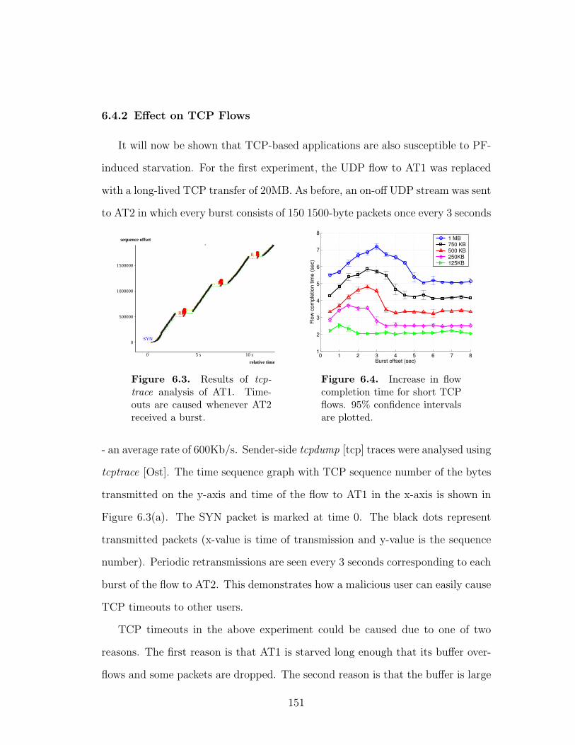
6.4.2 Effect on TCP Flows

It will now be shown that TCP-based applications are also susceptible to PF-

induced starvation. For the first experiment, the UDP flow to AT1 was replaced

with a long-lived TCP transfer of 20MB. As before, an on-off UDP stream was sent

to AT2 in which every burst consists of 150 1500-byte packets once every 3 seconds

1500000

1000000

500000

0

10 s 5 s 0

sequence offset

relative time

.�

�

�

�

�

��

�

3�

RRRRRRRRRRRRRRR�

RRRRRRR�

�

��

�

�

�

�

�

��

�

�

�

�

�

�

�

�3�

�

RRRRRRRRRRRRRRRRRRRRRR�

RRRRRR�

�

�

�

�

�

�

�

�

�

�

�

��

�

�

�

�

�3�

RRRRRRRRRRRRRRRRRR�

RRRRRRR�

RRRRRRRRRRRRRRRRRR�

�

��

�

�

�

�

�

�

�

�

�

�

�

�

�

�

�

�SYN�

Figure 6.3. Results of tcp-trace analysis of AT1. Time-outs are caused whenever AT2received a burst.

0 1 2 3 4 5 6 7 81

2

3

4

5

6

7

8

Burst offset (sec)

Flow

com

plet

ion

time

(sec

)

1 MB750 KB500 KB250KB125KB

Figure 6.4. Increase in flowcompletion time for short TCPflows. 95% confidence intervalsare plotted.

- an average rate of 600Kb/s. Sender-side tcpdump [tcp] traces were analysed using

tcptrace [Ost]. The time sequence graph with TCP sequence number of the bytes

transmitted on the y-axis and time of the flow to AT1 in the x-axis is shown in

Figure 6.3(a). The SYN packet is marked at time 0. The black dots represent

transmitted packets (x-value is time of transmission and y-value is the sequence

number). Periodic retransmissions are seen every 3 seconds corresponding to each

burst of the flow to AT2. This demonstrates how a malicious user can easily cause

TCP timeouts to other users.

TCP timeouts in the above experiment could be caused due to one of two

reasons. The first reason is that AT1 is starved long enough that its buffer over-

flows and some packets are dropped. The second reason is that the buffer is large

151

enough but AT1’s packets are delayed long enough that TCP experiences a spuri-

ous timeout. It turns out that per-AT buffers in EV-DO base stations are usually

80 to 100KB in size, which is larger than the default TCP receiver window size of

64KB in Linux and Windows (other versions use 32KB and 16KB [Har]). This was

verified this using sender side tcpdump traces. It might be argued that the labora-

tory configuration causes more spurious timeouts because we have fewer hops than

typical Internet paths. In fact, our configuration reflects the common practice of

wireless providers in using split-TCP or TCP proxies [WZZ+06]. Moreover, as

wireless speeds go up, delays are only going to decrease.

Short Flows: The impact on TCP performance due to spurious timeouts caused

by a malicious user will now be studied. Let us first consider short TCP flows

for which flow completion times are the suitable performance metric. For these

experiments, UDP flow to AT1 is replaced with TCP transfers ranging from 125KB

to 1MB. Since short flows spend a significant fraction of time in slow start, At

is likely to be small early on. Hence, the starvation duration is likely to depend

on the offset of the burst from the start time of the TCP flow. To understand

this better, experiments were conducted for various values of the burst offsets. For

each offset and flow size, the experiment was repeated 30 times and the plot of the

average flow completion times is shown in Fig. 6.4. The following four observations

were made. First, for a large enough offset, the burst has no impact because the

TCP flow is already complete. Second, the probability of a timeout increases as

the offset increases. This confirms our intuition that, during slow start, At of

AT1 is smaller and hence, starvation duration is smaller. Maximum performance

impact is realized when the offset is 2 − 3 seconds. This is observed when we

plot the average number of retransmissions too (figure not shown here). Third,

152

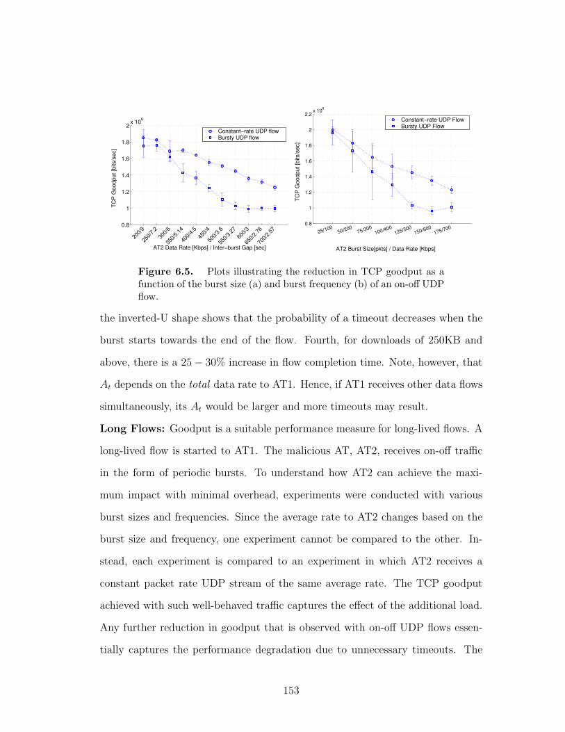
0.8

1

1.2

1.4

1.6

1.8

2 x 106

AT2 Data Rate [Kbps] / Inter−burst Gap [sec]

TCP

Goo

dput

[bits

/sec

]

200/9

250/7

.230

0/6

350/5

.14

400/4

.545

0/4

500/3

.6

550/3

.2760

0/3

650/2

.76

700/2

.57

Constant−rate UDP flowBursty UDP flow

0.8

1

1.2

1.4

1.6

1.8

2

2.2 x 106

AT2 Burst Size[pkts] / Data Rate [Kbps]

TCP

Goo

dput

[bits

/sec

]

25/10050/200

75/300100/400

125/500150/600

175/700

Constant−rate UDP FlowBursty UDP Flow

Figure 6.5. Plots illustrating the reduction in TCP goodput as afunction of the burst size (a) and burst frequency (b) of an on-off UDPflow.

the inverted-U shape shows that the probability of a timeout decreases when the

burst starts towards the end of the flow. Fourth, for downloads of 250KB and

above, there is a 25− 30% increase in flow completion time. Note, however, that

At depends on the total data rate to AT1. Hence, if AT1 receives other data flows

simultaneously, its At would be larger and more timeouts may result.

Long Flows: Goodput is a suitable performance measure for long-lived flows. A

long-lived flow is started to AT1. The malicious AT, AT2, receives on-off traffic

in the form of periodic bursts. To understand how AT2 can achieve the maxi-

mum impact with minimal overhead, experiments were conducted with various

burst sizes and frequencies. Since the average rate to AT2 changes based on the

burst size and frequency, one experiment cannot be compared to the other. In-

stead, each experiment is compared to an experiment in which AT2 receives a

constant packet rate UDP stream of the same average rate. The TCP goodput

achieved with such well-behaved traffic captures the effect of the additional load.

Any further reduction in goodput that is observed with on-off UDP flows essen-

tially captures the performance degradation due to unnecessary timeouts. The

153

average TCP goodput achieved in our experiments with on-off and well-behaved

UDP flows to AT2 are plotted in Figure 6.5. In the (a) plot, the inter-burst gap

for a burst size of 150 1500-byte packets was varied. As expected, the slope of

goodput with well-behaved UDP flows is almost linear with slope close to −1.

The performance impact of malicious behavior is clearly shown with the maxi-

mum reduction in goodput when the inter-burst gap is around 3 − 3.5 seconds.

In this case, the goodput reduces by about 400Kbps - almost 30%. Larger gaps

cause fewer timeouts and smaller gaps cause bursts to be sent before AT2’s At

has decayed to a small enough value. In the (b) plot, the burst size was varied for

a 3-second inter-burst gap. It was found that bursts of 125 − 150 packets cause

the largest reduction in goodput of about 25− 30%.

6.5 Parallel PF Algorithm

PF is vulnerable to “on-off” traffic primarily because it reduces A[t] (by mul-

tiplying it with 1 − α) even when an AT is not backlogged. A naive solution is

to freeze the value of A[t] for such ATs. But, a frozen A[t] value does not adapt

to changes in the number of backlogged ATs or channel conditions. Hence, an

AT with a recently unfrozen A[t] can have a ratio that is much lower or higher

than other ATs thereby causing starvation. A backlog-unaware algorithm, which

always considers ATs to be backlogged, is also not desirable since it would allocate

slots to ATs with no data to receive and hence, would not be work conserving.

We propose the following Parallel PF (PPF) algorithm that uses a backlog-

unaware scheduler instance only to remove the undue advantage an “on-off” user

receives at the beginning of “on” periods. A normal instance of PF drives slot

allocation. The parallel instance of PF assumes all ATs are backlogged and ex-

154

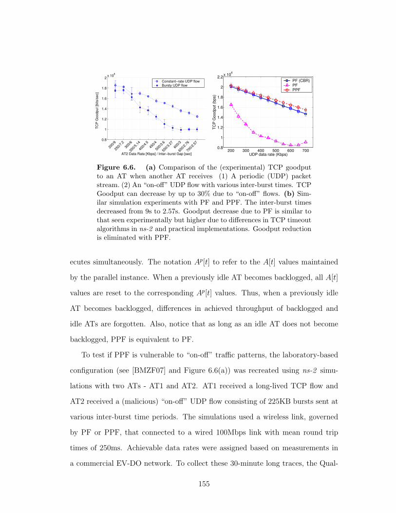
0.8

1

1.2

1.4

1.6

1.8

2 x 106

AT2 Data Rate [Kbps] / Inter−burst Gap [sec]

TCP

Goo

dput

[bits

/sec

]

200/9

250/7

.230

0/6

350/5

.14

400/4

.545

0/4

500/3

.6

550/3

.2760

0/3

650/2

.76

700/2

.57

Constant−rate UDP flowBursty UDP flow

200 300 400 500 600 7000.8

1

1.2

1.4

1.6

1.8

2

2.2 x 106

UDP data rate (Kbps)

TCP

Goo

dput

(bps

)

PF (CBR)PFPPF

Figure 6.6. (a) Comparison of the (experimental) TCP goodputto an AT when another AT receives (1) A periodic (UDP) packetstream. (2) An “on-off” UDP flow with various inter-burst times. TCPGoodput can decrease by up to 30% due to “on-off” flows. (b) Sim-ilar simulation experiments with PF and PPF. The inter-burst timesdecreased from 9s to 2.57s. Goodput decrease due to PF is similar tothat seen experimentally but higher due to differences in TCP timeoutalgorithms in ns-2 and practical implementations. Goodput reductionis eliminated with PPF.

ecutes simultaneously. The notation Ap[t] to refer to the A[t] values maintained

by the parallel instance. When a previously idle AT becomes backlogged, all A[t]

values are reset to the corresponding Ap[t] values. Thus, when a previously idle

AT becomes backlogged, differences in achieved throughput of backlogged and

idle ATs are forgotten. Also, notice that as long as an idle AT does not become

backlogged, PPF is equivalent to PF.

To test if PPF is vulnerable to “on-off” traffic patterns, the laboratory-based

configuration (see [BMZF07] and Figure 6.6(a)) was recreated using ns-2 simu-

lations with two ATs - AT1 and AT2. AT1 received a long-lived TCP flow and

AT2 received a (malicious) “on-off” UDP flow consisting of 225KB bursts sent at

various inter-burst time periods. The simulations used a wireless link, governed

by PF or PPF, that connected to a wired 100Mbps link with mean round trip

times of 250ms. Achievable data rates were assigned based on measurements in

a commercial EV-DO network. To collect these 30-minute long traces, the Qual-

155

0 1 2 3 4 5 6 7 8 91

1.5

2

2.5

3

3.5

4

4.5

5

5.5

6

Burst offset (sec)

Flow

com

plet

ion

time

(sec

)

Flow completion time: short flows

PF, 1MBPPF, 1MBPF, 750KBPPF, 750KBPF, 500KBPPF, 500KBPF, 250KBPPF, 250KBPF, 225KBPPF, 225KB

Figure 6.7. TCP flow completion times with PF and PPF sched-ulers. Measurement driven ns-2 simulations were used to plot theseresults.

comm CDMA Air Interface Tester [CDM06] software was used on a stationary

AT and a mobile AT moving at an average speed of 40mph. The TCP goodput

obtained with PF and PPF is plotted in Figure 6.6 (b). The results clearly show

that, with PPF, the TCP goodput is not affected by the “on-off” flow. This is the

reason why the TCP goodput with PPF is slightly higher than the goodput with

PF and a CBR flow consisting of periodically-sent UDP packets. To understand

how much improvement in flow-completion times of short flows can be obtained

by replacing PF scheduler with PPF scheduler the laboratory experiment deis-

cussed earlier in Section 6.4 was recreated using ns-2. Improvement in short flow

completion times can be seen in Figure 6.7. As expected, using PPF reduces the

flow completion times of short flows.

The proposed PPF algorithm uses the achievable rate feedback from the ATs

156

to maintain parallel values of the average rate and hence can work only when

data rate values are reported by the ATs. The connection timer at the AT expires

after about 12 seconds of inactivity and the AT stops reporting its achievable rate

values to the base station. When new data arrives for the AT, a new connection

is established between the core network and the AT and the average is reset to

0 again. This AT gets all the time slots for some time, starving all other ATs

despite there being a PPF scheduler to reduce the starvation. To overcome this

problem, we propose an algorithm that allows the average to grow quickly and

converge to a value such that sharing between ATs can begin. This is achieved

by not having a fixed value of the parameter α but instead having the value of α

shrink from α = 1 down to α = 11000

. For the first time slot when new data to

the AT arrives and a new connection is established, value of α equals 1 and the

average is 0. In the second time slot, α = 12, in the third, α = 1

3and so on. After

1000 slots, the value of α is 11000

and it does not shrink after this. This method

of updating the value of α allows the average to change faster than it would have

had the value of α been fixed at 11000

.

6.6 Summary

Proportional fair scheduler is commonly used for downlink scheduling by most

3G wireless equipment makers and is widely deployed. The contribution of this

work is the finding that PF can be easily corrupted, accidentally or deliberately

causing real-time multimedia impairments. Scheduler induced impairments were

rigorously quantified in this work using experiments conducted in both laboratory

and production network settings. It was observed that the delay jitter can be

increased by as much as 1 second and TCP throughput can be reduced by as much

157

as 25-30 % by a single malicious user. An important contribution of this work is a

new scehduling algorithm (the parallel proportional fair scheduler) that mitigates

the scheduler-induced impairments. It is shown using ns-2 simulations that the

new scheduler significantly reduces the impairments and improves the throughput

and delay performance. The parallel scheduler however cannot work when the

AT’s session transitions to an inactive state as in this state, the instantaneous

channel conditions are not reported by the AT using the DRC channel. The

shrinking alpha algorithm proposed in this work can be used then to change the

average rates faster allowing impairments to be reduced significantly.

158

Chapter 7

Conclusions and Future Work

7.1 Conclusions

Improving network function by matching response to network conditions (or

the estimate of network conditions) is not a new idea and has been used in the

Internet for decades. For example, TCP uses packet loss feedback and end system

available buffer size feedback to adjust the sending rate. New methods for im-

proving network functions are using the same basic idea of matching the response

to network conditions. For example, TCP optimizers for wireless networks (e.g.,

optimizers from Bytemobile [Byt] and Venturi Wireless [Wir]) split the end-to-end

TCP connection into wired and wireless parts. In the wireless part, these opti-

mizers use core-to-end active measurements to estimate the available bandwidth

and wireless channel conditions and match the sending rate accordingly with the

main goal of improving TCP throughput. Cross layer measurement based opti-

mizers (like the one by Mobidia [Mob]) use cross-layer measurement input of the

radio conditions to improve network functions at layer 3 and above. To apply

the correct response, it is important to first accurately detect the correct network

159

condition using measurements. As the Internet evolves integrating new physical

layer technologies and algorithms the number of possible causes that result in sim-

ilar observable symptoms at the end node are increasing. For example, after the

invention and widespread deployment of BGP in the Internet, BGP convergence

delay has now been added to the list of network problems that may cause ob-

servable symptom of packet losses at the end node. Since the growing complexity

of the Internet is resulting in an increasing number of events to causing similar

observable symptoms at the end system, it is becoming important to develop ad-

vanced techniques to detect and identify these events. Also, due to the increasing

security and proprietary concerns, service providers are blocking more and more

information (e.g. ICMP blocking, SIP/IMS topology hiding [SBC]) that allowed

end systems to know more about their networks. The decrease in the amount of

information available at the end system to allow detection and identification of

network events strengthens the case for the development of advanced end-to-end

event detection and identification techniques.

Some of the main contributions of this work are the development of new meth-

ods for detection and identification of events like RTM impairments, congestion

and route changes using only the delay and loss information. Burst loss, discon-

nected, high random loss and high delay RTM impairment events were defined

and methods to detect these events from delay and loss time series were developed.

Using 26 days of PlanetLab data collected over 9 different end node pairs it was

found that mean time between RTM impairments varied from 3.5 hours to 268

hours depending on the path and the mean duration of impairments varied from 4

minutes to 92 minutes for different node pairs. Metrics like time between and du-

ration of impairments provide the end users information about the network that is

160

very understandable. It is demonstrated using PlanetLab measurements that the

methods developed in this dissertation can be used to detect RTM impairments.

Also, the RTM impairments observed on these paths were correlated with the con-

gestion and route change events to illustrate what type of impairment events are

caused by these network events. Heuristic-based methods for detecting conges-

tion and route changes from delay and loss information were also developed and

evaluated using the same PlanetLab measurement data. Congestion was detected

on two of the nine paths and on these paths it occurred for 6-8 hours during the

day on weekdays. Route changes were observed on all the nine paths over which

measurements were conducted. Mean duration of loss impairments that occurred

just before route changes (113.5 sec) was found to be five times longer than the

mean duration of loss impairment that occurred during congestion (22.64 sec).

The details of all the results from this measurement study are discussed in section

2.4.

From the PlanetLab measurement study, it was found that the heuristics-

based route change detection algorithm was able to detect 71% of all visible layer

2 route changes. Route changes that occurred too close together in time or the

ones for which the minimum RTT changed by less than 0.5 ms could not be de-

tected. A model-based optimal detector (PAD) was developed and analysed to

find out how close the performance of heuristics-based algorithm is to the best

possible performance. ROC curves were used to compare the simulated and the

predicted performance and to show that the analysis developed in this disserta-

tion accurately predicts the performance. Although the PAD is ideal, it cannot

be implemented in practice because of the assumption that the parameters are

known in advance. A practical model-based algorithm (PUD) was also developed

161

here to find out if the model-based approach can be used to design a detector

that performs better than the heuristics-based detector. Extensive simulations

were conducted to find the region of the parameter space over which the three

algorithms have acceptable performance (where acceptable performance is defined

as PD ≥ 0.999 and PF ≤ 0.001). The region of acceptable performance is largest

for the PAD as expected, followed by PUD and then by the heuristics-based de-

tector. This shows that the model-based detector has accpetable performance

over a larger set of parameter values than the heuristics-based detector and may

be the preferred practical detector for this reason. The PUD was also applied

to measured RTT data from PlanetLab to evaluate the algorithm on network

measurements.

Another very important contribution of this work is the discovery that the

widely deployed PF scheduler can be easily corrupted, accidentally or deliber-

ately, to starve flows and cause RTM impairments in wireless networks. In this

dissertation, field experiments were used to rigorously quantify the impact of star-

vation observable at the transport layer. A combination of both laboratory and

production network measurements were used in this study to demonstrate the PF

starvation vulnerability. It is shown using measurements that the delay jitter can

be increased to 1 second and the TCP throughput can be decreased by as much as

25-30% by a single malicious user. The analysis for predicting starvation duration

when the channel conditions are fixed was also developed and validated. Inter-

burst gap and burst duration were varied to find the parameter values at which

an attacker can cause maximum damage and it was found that this malicious AT

can reduce TCP throughput by 25-30%. A parallel PF algorithm was proposed

to mitigate the starvation vulnerability of the PF algorithm. It was shown using

162

ns2 simulations that when the parallel PF algorithm is used instead of the PF

algorithm, the malicious user is not able to starve any flows. Also, the parallel

PF is a variant of the PF algorithm and for this reason it has the same through-

put optimality and fairness properties as PF. Since parallel PF algorithm requires

that inactive ATs should keep on reporting their achievable rates and since ATs

stop reporting achievable rates after a few seconds of inactivity, flows can still be

starved when ATs come on after long periods of inactivity. An adaptive alpha

updating mechanism was designed to deal with this problem and it was shown

that the flow starvation problem can be mitigated by using this new algorithm.

7.2 Future Work

Probability of detection and false alarms for the PAD can be predicted very

accurately using the analysis developed in this dissertation. However, the PAD

is the ideal detector and the requirement that the parameter values should be

known in advance limits its applicability. The analysis developed for PAD was

used to predict the performance bounds for all detectors. The performance curves

for PUD were obtained using extensive simulations because the analysis for PUD

was not developed. Since PUD is based on the assumption that the parameters of

Gamma distribution are not known but are estimated, the analysis for predicting

the performance of PUD is more complicated than the one for PAD. Note that

for PUD, the right hand side of Equation 3.3 has parameter estimates instead of

the parameter values (like in PAD). Since the parameter estimated of the three

parameter Gamma distribution are random variables whose mapping function is

non-trivial, this analysis is more complicated. However some simplifying assump-

tions may lead to analytical expressions for predicting the performance of the

163

PUD. This analysis for predicting performance of PUD is not just of academic

interest but also has practical significance because it can be used to find the op-

timal decision threshold for any given set of parameter values. It has already

been shown in this work that PUD is the practical detector of choice because of

its performance advantage over the heuristic detector and with the performance

prediction analysis PUD can predict optimal thresholds in real time since it does

not take much computations to predict the optimal threshold using the analysis.

Although PAD cannot be used in practice in most cases because the parameter

values are not known in advance, it may be possible to use PAD in some cases

like for detecting route flapping between two paths. If there is persistent route

flapping between two paths, the detector can learn the parameter values of both

paths over time. After some time, when the detector has collected enough samples

from both paths and has gained enough confidence in the parameter estimates of

both paths, PAD can be applied to detect route changes because the detector is

already aware of the parameter values of both paths. The design issues like how

many samples to collect before applying PAD and how to detect that the route

flapping has stopped so as to stop applying PAD and start using PUD can be

explored in future work.

164

References

[ABBM03] H. Kaplan A. Bremler-Barr, E. Cohen and Y. Mansour. Predict-

ing and bypassing end-to-end Internet service degradations. IEEE

Journal on Selected Areas in Communications, 21(6):961–978, June

2003.

[AMD04] S. Bhattacharyya C. Chuah A. Markopoulou, G. Iannaccone and

C. Diot. Characterization of failures in an ip backbone. In Proceed-

ings of IEEE INFOCOM 2004, pages 2307–2317, Hong Kong, March

2004.

[AZJ03] Z. Wang A. Zeitoun and S. Jamin. Rttometer: Measuring path min-

imum rtt with confidence. In Proceedings of 3rd IEEE Workshop

on IP Operations and Management (IPOM 2003), pages 127–134,

Kansas City, USA, October 2003.

[BCL+04] Tom Beigbeder, Rory Coughlan, Corey Lusher, John Plunkett, Em-

manuel Agu, and Mark Claypool. The effects of loss and latency on

user performance in unreal tournament 2003. In Proceedings of ACM

SIGCOMM 2004 Workshops on NetGames ’04, pages 144–151, 2004.

165

[BJFD05] Soshant Bali, Yasong Jin, Victor S. Frost, and Tyrone Duncan. Char-

acterizing user-perceived impairment events using end-to-end mea-

surements. Accepted for publication in International Journal of Com-

munication Systems, 2005.

[BK46] M. S. Bartlett and D. G. Kendall. The statistical analysis of variance

heterogeneity and logarithmic transformation. Journal of the Royal

Statistical Society, 8:128–138, 1946.

[BMZF07] S. Bali, S. Machiraju, H. Zang, and V. Frost. A Measurement Study

of Scheduler-based Attacks in 3G Wireless Networks. In Proc. of

Passive and Active Measurement (PAM) Conference, 2007.

[BSUB98] M. Borella, D. Swider, S. Uludag, and G. Brewster. Internet packet

loss: measurement and implications for end-to-end QoS. In ICPPW

’98: Proceedings of the 1998 International Conference on Parallel

Processing Workshops, pages 3–15, 1998.

[Byt] Bytemobile. http://www.bytemobile.com/.

[CBD02] G. Iannaccone C. Boutremans and C. Diot. Impact of link failures on

voip performance. In Proceedings of the 12th International Workshop

on Network and Operating Systems Support for Digital Audio and

Video, pages 63–71, Miami, Florida, USA, May 2002.

[CDM06] CDMA Air Interface Tester. http://www.cdmatech.com/download_

library/pdf/CAIT.pdf, 2006.

[CHNY02] Mark Coates, Al Hero, Robert Nowak, and Bin Yu. Internet tomog-

raphy. IEEE Signal Processing Magazine, 19:47–65, 2002.

166

http://www.bytemobile.com/

http://www.cdmatech.com/download_library/pdf/CAIT.pdf

http://www.cdmatech.com/download_library/pdf/CAIT.pdf

[CJT04] Y. Levy F. Saheban C.R. Johnson, Y. Kogan and P. Tarapore. VoIP

reliability: A service provider’s perspective. IEEE Communications

Magazine, 42(7):48–54, July 2004.

[CMR03] L. Ciavattone, A. Morton, and G. Ramachandran. Standardized

active measurements on a tier 1 ip backbone. IEEE Communications

Magazine, 41:90–97, 2003.

[CT99] M. Claypool and J. Tanner. The effects of jitter on the perceptual

quality of video. In Proceedings of ACM Multimedia Conference,

pages 115–118, Orlando, Florida, USA, November 1999.

[Don01] Sean Donelan. Internet outage trends. http://www.nanog.org/mtg-

0102/donelan.html, Feb. 2001. NANOG meeting.

[DP00] Nick G. Duffield and Francesco Lo Presti. Multicast inference of

packet delay variance at interior network links. In Proceedings of

IEEE INFOCOM 2000, Tel-Aviv, Israel, March 2000.

[DP04] N.G. Duffield and F.L. Presti. Network tomography from measured

end-to-end delay covariance. IEEE/ACM Transactions on Network-

ing, 12:978–992, 2004.

[DPZ03] D. Massey S. F. Wu D. Pei, L.Wang and L. Zhang. A study of

packet delivery during performance during routing convergence. In

Proceedings of IEEE/IFIP International Conference on Dependable

Systems and Networks (DSN), 2003.

167

[FHPW00] Sally Floyd, Mark Handley, Jitendra Padhye, and Jorg Widmer.

Equation-based congestion control for unicast applications. In SIG-

COMM 2000, pages 43–56, Stockholm, Sweden, August 2000.

[Fro03] Victor S. Frost. Quantifying the Temporal Characteristics of Network

Congestion Events for Multimedia Services. IEEE Transactions on

Multimedia, 5(4):458–465, Aug. 2003.

[G.103] ITU-T Recommendation G.114, May 2003.

[GID02] R. Mortier S. Bhattacharyya G. Iannaccone, C. Chuah and C. Diot.

Analysis of link failures in an ip backbone. In Proc. Of 2nd ACM

SIGCOMM Internet Measurement Workshop, pages 237–242, Mar-

ceille, France, November 2002.

[Gil03] G. Hudson Gilmer. The real-time IP network: moving IP networks

beyond best effort to deliver real-time applications, 2003. AVICI

Systems white paper.

[Har] Carl Harris. Windows 2000 TCP Performance Tuning Tips http:

//rdweb.cns.vt.edu/public/notes/win2k-tcpip.htm.

[HC95] R. V. Hogg and A. T. Craig. Introduction to Mathematical Statistics.

Prentice-Hall, fifth edition, 1995.

[ICBD04] Gianluca Iannaccone, Chen-Nee Chuah, Supratik Bhattacharyya,

and Christophe Diot. Feasibility of IP restoration in a tier-1

backbone. IEEE Networks Magazine, Special Issue on Protection,

Restoration and Disaster Recovery, 2004.

168

http://rdweb.cns.vt.edu/public/notes/win2k-tcpip.htm

http://rdweb.cns.vt.edu/public/notes/win2k-tcpip.htm

[ICM+02] G. Iannaccone, C. Chuah, R. Mortier, S. Bhattacharyya, and C. Diot.

Analysis of link failures in an IP backbone. In Proc. of ACM SIG-

COMM Internet Measurement Workshop, Nov 2002.

[Isw] Iswest sdsl service level agreement.

http://www.iswest.com/serviceagree-ment.html.

[JBG04] J.H.James, Chen Bing, and L Garrison. Implementing VoIP: A Voice

Transmission Performance Progress Report. IEEE Communications

Magazine, 42(7):36–41, July 2004.

[JCBG95] H. Crepin J.-C. Bolot and A.V. Garcia. Analysis of audio packet loss

in the internet. In Proceedings of the 5th International Workshop on

Network and Operating System Support for Digital Audio and Video,

pages 154–165, Durham, NH, USA, April 1995.

[JJG04] C. Bing J.H. James and L. Garrison. Implementing VoIP: A voice

transmission performance progress report. IEEE Communications

Magazine, 42(7):36–41, July 2004.

[JPP00] A. Jalali, R. Padovani, and R. Pankaj. Data Throughput of CDMA-

HDR: A High Efficiency-high Data Rate Personal Communication

Wireless System. Proc. of IEEE Vehicular Technology Conference,

3:1854–1858, May 2000.

[JS00] W. Jiang and H. Schulzrinne. QoS measurement of Internet real-time

multimedia services. In Proceedings of NOSSDAV, Chapel Hill, NC,

June 2000.

169

[JS02] W. Jiang and H. Schulzrinne. Comparison and optimization of packet

loss repair methods on voip perceived quality under bursty loss. In

NOSSDAV ’02: Proceedings of the 12th International Workshop on

Network and Operating Systems Support for Digital Audio and Video,

pages 73–81, Miami Beach, FL, USA, May 2002.

[Kle75] L. Kleinrock. Queueing Systems Volume 1: Theory. Wiley, 1975.

[KPD03] R. Cruz K. Papagiannaki and C. Diot. Network performance mon-

itoring at small time scales. In IMC ’03: Proceedings of the 3rd

ACM SIGCOMM Conference on Internet Measurement, pages 295–

300, Miami Beach, Florida, October 2003.

[KPH04] D. Veitch K. Papagiannaki and N. Hohn. Origins of microconges-

tion in an access router. In Proc. Passive and Active Measurment

Workshop, Antibes Juan-Ies-Pins, France, April 2004.

[KR02] R. Koodli and R. Ravikanth. One-way loss pattern sample metrics.

In RFC 3357, Internet Engineering Task Force, 2002.

[LABJ00] Craig Labovitz, Abha Ahuja, Abhijit Bose, and Farnam Jahanian.

Delayed Internet routing convergence. In Proceedings of ACM SIG-

COMM, pages 175–187, 2000.

[LAJ98] C. Labovitz, A. Ahuja, and F. Jahanian. Experimental study of

Internet stability and wide-area backbone failures. Technical Report

CSE-TR-382-98, University of Michigan, 1998.

[Law82] J. F. Lawless. Statistical Models and Methods for Lifetime Data.

Wiley, 1982.

170

[MCN02] R. Castro M. Coates and R. Nowak. Maximum likelihood network

topology identification from edge-based unicast measurements. ACM

Sigmetrics Performance Evaluation Review, 30(1):11–20, June 2002.

[ME98] W. Q. Meeker and L.A. Escobar. Statistical Methods for Reliability

Data. Wiley, 1998.

[MEP93] N. Hastings M. Evans and B. Peacock. Statistical distributions. Wi-

ley, 2nd edition, 1993.

[MKT98] Sue B. Moon, Jim Kurose, and Don Towsley. Packet Audio Playout

Delay Adjustment: Performance Bounds and Algorithms. Multime-

dia Systems, 6(1):17–28, 1998.

[MMS05] I. Saniee M. Mandjes and A. Stolyar. Load Characterization and

Anomaly Detection for Voice Over IP Traffic. IEEE Transactions on

Neural Networks, 16(5):1019–1026, September 2005.

[Mob] Mobidia. http://www.mobidia.com/.

[MT00] V. Markovski and L. Trajkovic. Analysis of loss episodes for video

transfer over UDP. In Proceedings of the SCS Symposium on Per-

formance Evaluation of Computer and Telecommunication Systems

(SPECTS’2K), pages 278–285, 2000.

[MTK03] Athina P. Markopoulou, Fouad A. Tobagi, and Mansour J. Karam.

Assessing the Quality of Voice Communications over Internet Back-

bones. IEEE/ACM Transactions on Networking, 11(5):747–760,

2003.

171

http://www.mobidia.com/

[Muk92] Amarnath Mukherjee. On the dynamics and significance of low fre-

quency components of internet load. Technical Report MS-CIS-92-83,

University of Pennsylvania, December 1992.

[MYT99] J.F. Kurose M. Yajnik, S.B. Moon and D.F. Towsley. Measurement

and modeling of the temporal dependence in packet loss. In Proceed-

ings of IEEE INFOCOM 1999, pages 345–352, New York, NY, USA,

March 1999.

[NC04] James Nichols and Mark Claypool. The effects of latency on online

Madden NFL football. In NOSSDAV ’04: Proceedings of the 14th

International Workshop on Network and Operating Systems Support

for Digital Audio and Video, pages 146–151, 2004.

[NGDD02] J. Horowitz Nicholas G. Duffield, Francesco Lo Presti and D.Towsley.

Multicast topology inference from measured end-to-end loss. IEEE

Transactions on Information Theory, 48(1):26–35, Jan 2002.

[NJB94] S. Kotz N.L. Johnson and N. Balakrishnan. Continuous univariate

distributions : Vol. 1. John Wiley, New York, 2nd edition, 1994.

[Ost] Shawn Ostermann. tcptrace, http://jarok.cs.ohiou.edu/

software/tcptrace.

[pla04] Timing problem on planetlab (bad NTP). http://lists.planet-

lab.org/pipermail/users/2004-March/000050.html, March 2004.

[PW02] Lothar Pantel and Lars C. Wolf. On the impact of delay on real-

time multiplayer games. In NOSSDAV ’02: Proceedings of the 12th

172

http://jarok.cs.ohiou.edu/software/tcptrace

http://jarok.cs.ohiou.edu/software/tcptrace

International Workshop on Network and Operating Systems Support

for Digital Audio and Video, pages 23–29, 2002.

[RHdB05] G. Karagiannis J. Loughney R. Hancock, I. Freytsis and S. Van den

Bosch. Next steps in signaling: Framework. In RFC 4080, Internet

Engineering Task Force, June 2005.

[SB88] K. Sam Shanmugan and Arthur M. Breipohl. Random Signals: De-

tection, Estimation and Data Analysis. John Wiley & Sons Inc.,

1988.

[SBC] Acme Packet SBC. http://www.acmepacket.com/.

[SSLB05] Charles Shen, H. Schulzrinne, Sung-Hyuck Lee, and Jong Ho Bang.

Routing dynamics measurement and detection for next step inter-

net signaling protocol. In Proc. of 2005 Workshop on End-to-End

Monitoring Techniques and Services, Nice, France, May 2005.

[tcp] tcpdump. http://www.tcpdump.org.

[TKM98] I. Sidhu G.M. Schuster J. Grabiec T.J. Kostas, M.S. Borella and

J. Mahler. Real-time voice over packet-switched networks. IEEE

Network, 12(1):18–27, Jan/Feb 1998.

[UHD02] R. Mortier U. Hengartner, S. Moon and C. Diot. Detection and

analysis of routing loops in packet traces. In Proceedings of the 2nd

ACM SIGCOMM Workshop on Internet Measurement, pages 107–

112, Marseille, France, November 2002.

173

http://www.acmepacket.com/

http://www.tcpdump.org

[VTL02] P. Viswanath, D. Tse, , and R. Laroia. Opportunistic Beamforming

using Dumb Antennas. IEEE Transactions on Information Theory,

48:1277–1294, June 2002.

[WHZ00] Dapeng Wu, Yiwei Thomas Hou, and Ya-Qin Zhang. Transport-

ing Real-Time Video over the Internet: Challenges and Approaches.

Proceedings of the IEEE, 88(12):1855 – 1877, 2000.

[Wir] Venturi Wireless. http://www.venturiwireless.com/.

[WJS03] K. Koguchi W. Jiang and H. Schulzrinne. Qos evaluation of voip

end-points. In Proceedings of the IEEE International Conference on

Communications, pages 1917–1921, Anchorage, AL, USA, May 2003.

[WWTK03] W. Wei, B. Wang, D. Towsley, and J. Kurose. Model-based identifica-

tion of dominant congested links. In Proceedings of the 3rd ACM SIG-

COMM conference on Internet Measurement, Miami Beach, Florida,

October 2003.

[WZZ+06] W. Wei, C. Zhang, H. Zang, J. Kurose, and D. Towsley. Inference

and Evaluation of Split-Connection Approaches in Cellular Data Net-

works. In pam, 2006.

[XY06] Wang Xiaoyi and Qu Yajiang. Enhanced proportional fair scheduling

for cdma2000 1x ev-do reverse link. In Wireless and Optical Com-

munications Networks, 2006 IFIP International Conference on, April

2006.

[YT03] Shing Yin and Ken Twist. The coming era of absolute availability.

http://www.chiaro.com/pdf/rhk.pdf, May 2003. RHK white paper.

174

http://www.venturiwireless.com/

[ZDPS01] Y. Zhang, N. Du, V. Paxson, and S. Shenker. On the constancy of

Internet path properties. In Proceedings of ACM SIGCOMM Internet

Measurement Workshop, San Francisco, California, USA, November

2001.

175

detection and mitigation of impairments for real-time ... · detection and mitigation of...

Documents