detection and quantification of pcb in soil using gc/ms
TRANSCRIPT

Detection and Quantification of PCB in
soil using GC/MS
- method development and education for users
Elias Saba
Master Thesis for the program Civilingenjör och Lärare in math and chemistry
Stockholm 2012

- 1 -
External Supervisor: Rune Öhrn, Laboratory Manager, Vesta Ceramics AB (formerly Ljungalab AB), Ljungaverk, Sweden
Main Supervisor: Åsa Emmer, Division of Analytical chemistry, department of Chemistry, School of Chemical Science and Engineering, KTH Royal Institute of technology
Assistant Supervisor: Lena Geijer, Institution for pedagogics and didactics, Department of Education/Stockholms University, Stockholm
Examiner: Catharina Silfverbrand Lindh, Ingenjörspedagogiska enheten, department of Engineering and Pedagogics, School of Chemical Science and Engineering, KTH Royal Institute of technology

- 2 -
Abstract:
The aim of this paper is to document the development of a method for detection and quantification of Polychlorinated biphenyls (PCB) in soil using Gas Chromatography (GC) connected to a Quadrupole Mass Spectrometer (MS) via an internal standard (CB189). The method developed is performed in conjunction with the information provided by the Swedish environmental agency (Svenska naturvårdsverket, SNV) in regards to PCB limits for sensitive land usage. The steps of the method and maintenance of the GC/MS are used to create a user manual and an attempt at transformative learning is done in an effort to teach the staff at LjungaLab AB so that at the very least, independent analysis can be run and at best, new methods and application are independently developed for the GC/MS. An evaluation of the teaching efforts is also done to assess what grade of learning is achieved.
Syftet med denna uppsats är att dokumentera utvecklingen av en metod för detektion och kvantifiering av polyklorerade bifenyler (PCB) i jord med hjälp av gaskromatografi (GC) ansluten till en masspektrometer (MS) och med användning av en intern standard (CB189). Metoden som utvecklats skapades med hjälp av uppgifter från det svenska naturvårdsverket (SNV) angående PCB-gränser för känslig markanvändning. Därefter skapades en användarmanual som beskriver stegen i metoden och även underhåll av GC/MS. Personalen på LjungaLab AB undervisades i hur man använder och underhåller instrumenten för att, åtminstone, kunna köra oberoende analyser, och i bästa fall, utveckla nya metoder och tillämpningar självständigt. Det sistnämda är ett försök till transformativ lärande. En utvärdering av lärarinsatser sker också för att bedöma vilken grad av lärande som uppnås.
Key words:
Transformative learning, GC, MS, PCB, teaching, pedagogics, detection, quantification, quadrupole MS, internal standard, chemical analysis, user manual, artefact, cognitivism, social constructivism.
Transformativ lärande, GC, MS, PCB, lärande, pedagogik, detektion, kvantifiering, kvadrupol MS, intern standard, kemisk analys, användamanual, artefakt, kognitivism, social konstruktivism.

- 3 -
Table of Contents Page
Abstract 2
Keywords 2
Introduction 5
The Scientific Aim 5
The Pedagogical Aim 5
Background of PCB 6
Theory 8
Introduction to the instruments 8
Calibration 10
Sample Calculation 10
Materials and Methods 12
Standards 12
Instrument Setup 13
Elution order and Retention Time 14
Processing method 14
Sample preparation 14
Results and Discussion 16
Fullscan vs SIM 16
Column Change 17
New column runs and choice between iso-octane or cyclo-
hexane as solvent 20
Internal Standard RT 24
Calibration and Process method 1 24
Calibration and Process method 2 26
Soil Samples and Reports 28

- 4 -
Pedagogics 30
Theoretical Framework 30
Transformative and Emancipatory Learning 30
Social Constructivism 30
Cognitivism 31
Method framework 31
Introduction 31
Method 32
Method Walkthrough 32
The Practical Problem 32
Observation and Assessment 32
Transfer of Knowledge 33
Outline of User Manuals 35
Results 36
Unknown Sample Runs - Worksheet 1 36
Calibration and Process method Modifications - Worksheet2
37
Analysis and Discussion 38
Conclusions and future development 39
References 41
Appendix 43
1. Hardware Maintenance – User Manual 43
2. PCB Analysis – User Manual 48
3. Worksheet 1 59
4. Worksheet 2 60

- 5 -
Introduction
The company LjungaLab AB is a small laboratory that is located in the north of Sweden, 80km west of the city Sundsvall. They have a broad assortment of techniques such as XRF (x-ray fluorescence) XRD (x-ray diffraction), LECO element determination, GC, GC-ECD (gas chromatography-electron capture detector), Rheology, pH, conductivity and titration among others and these services are provided to mainly other chemical industries. Looking to develop their techniques they have commissioned a task which involves using a new combination of instruments, the mass spectrometer (MS), which coupled with gas chromatography (GC) allows detecting and quantifying very low concentrations of a vast array of molecules. They require help with the development of an analytical method that quantifies PCB in soil at low concentrations (<0.008mg/kg1), which are in accordance with the SNV (Svenska naturvårdsverket/the Swedish environmental agency). They also require teaching of how to use and service the instruments and how to use the software that steers said instruments. The staff have little prior experience using the MS and the software so the person undertaking the task needs to first learn how to use the software, how to maintain the GC-MS, develop a working method to analyze PCB in soil, automate the procedure and thereafter begin to teach the staff how to use the software and how to maintain the instruments.
The Scientific Aim
There are two main aspects to the task at hand. One is the chemical analysis and method development for the GC-MS. This includes becoming competent with the software and comfortable enough to use it as to create both an instrument and process method that allows for analysis of PCB in soil. This includes running calibrations and tests and finding a useful method that can then be used to quantify the amount of PCB in soil. This also includes researching literature about prior methods developed for quantification of PCB and how to prepare and run standards.
The Pedagogical Aim
The second aspect to the task is finding useful pedagogical model(s) to teach the staff how to run the instruments and maintain them in working order. Here, a few different pedagogical theories such as Piagets cognitivism, Vygotskijs social constructivism and also Mezirows theories toward transformative learning and emancipatory education are used. The sociocultural aspect that needs to be understood is that culture is dynamic and must be studied in order to ascertain how best to teach these adults. Also understanding how the tools are used, in this case the software and hardware, is central for their understanding and would then enable to push their intellectual and practical capabilities to encompass using the
1 http://www.naturvardsverket.se/Start/Produkter-och-avfall/PCB-i-byggnader-och-utrustning/Till-dig-som-utovar-tillsyn-kopplat-till-PCB/ , retrieved 2012-06-29
- 6 -
GC-MS. It is important to observe how they interact with each other and allow the group to also learn from each other. In Mezirows theory it is imperative to foster critical reflection to finally reach transformative learning and for this to occur there must first be meaning in what is being done and reflection to examine the meaning, thereupon critical reflection, which is an independent process, assesses the validity of the proposed learning to finally being comfortable enough to go out on their own and reach transformative learning which according to Mezirow “can take place without professional interventions”. My role as educator is to create enough rapport with my students to promote learning in a sociocultural environment and produce material (artefacts) which allows them to use and maintain the instruments, to guide them in a manner suited to their culture and to observe them working on their own to make sure that learning is occurring. My final and hardest task is to attempt to generate a high level of transformative learning which for example would be by development of new analytical methods using the GC/MS which I hope can be accomplished with the information compiled in the form of user manuals.
Background of PCB
PCB is an environmental toxin that is extremely stable and gets concentrated as it moves up the food chain due to its fat soluble properties. It has been found all over the world in both living and non-living matter (Büthe 1994). One of the reasons for this is that PCB is an extremely stable molecule that survives high temperatures and is difficult to reduce or oxidize (Boate 2004), thus destruction of waste containing PCB has caused it to be spread in the atmosphere.
In the 60s dichlorodiphenyltrichloroethane (DDT) and Mercury (Hg) were recognized as toxic to the environment (Bernes Monitor 16). Further chemical analysis of different independent DDT samples showed 14 unidentified substances in high concentrations. In 1966 Sören Jensen found that these unidentified substances were compounds consisting of chlorine and biphenols, PCB was discovered and had already become as widespread as pesticides and heavy metals that were purposefully placed in nature2. This had alarmed many countries and rules and regulations were put into place that limited the usage and disposal of PCB during the 70s, which in turn has caused the levels of PCB in nature to decline. An example of this is that the concentration of PCB per gram fat in herring eggs had declined from 350ug/g in 1975 to under 50ug/g in 1995 (Åsterbro 1999).
The Swedish environmental agency (Svenska Naturvårdsverket, SNV) have set up limits to how high concentration of PCB is allowed to be in certain areas3 and the need for efficient analysis of samples taken from these areas are on the rise. The Swedish environmental agency has decided that the detection and sum of 7
2 http://www.sanerapcb.nu/web/page.aspx?refid=4 , retrieved 2012-06-29 3 http://www.naturvardsverket.se/sv/Start/Verksamheter-med-miljopaverkan/Fororenade-omraden/Att-utreda-och-efterbehandla-fororenade-omraden/Riktvarden-for-fororenad-mark/Tabell-over-generella-riktvarden/ , retrieved 2012-06-29

- 7 -
specific congeners of PCB should be no more than 0.008mg/kg for sensitive land usage (schools, offices, residential areas).
The acute toxicity of PCB is low; however, as it gets more concentrated up the food chain, the dangers increase. PCB gets stored in fat tissue of living animals and studies show that dangerous long term effects include embryo toxicity, immunosupression and neurological degeneration (Bernes Monitor 16).

- 8 -
Theory
There are 209 theoretical PCB congeners of which 140 are found in different industrial PCB mixtures that were produced for among other things plastic softeners. These different congeners were numbered and described by Ballschmitter (Ballschmitter 1992). The detection and quantification of PCB in nature has been done in a plethora of ways depending on the matrix the PCB is in. To perform a chemical analysis properly, certain steps must be followed; sampling, reprocessing/extraction of PCB using solvents, instrumental analysis and evaluation. Also, the analysis instrument (GC/MS) must be regularly calibrated in order to eliminate errors and to make sure that the instrument is in working order as they tend to degrade over time. The method of separation and detection chosen is with a wall-coated open-tubular GC column (WCOT) connected to a quadrupole MS. The WCOT separates the different PCB congeners during the oven temperature programming and the MS then detects them using selected ion monitoring (SIM). The quantification is done using the software Xcalibur® via the use of standards for calibration. The calibration is accomplished by using varying concentrations of 7 different PCB congeners with a constant concentration of a specific PCB congener as the internal standard (CB189). This congener is an ideal candidate since it is not found in industrial mixtures of PCB which means it is not going to be in soil samples contaminated with PCB. The choice for the detection and quantification of these 7 PCB congeners is done in conjunction with SNVs guidelines for the limit of PCB in soil. These 7 PCB congeners (CB’s: 28, 52, 101, 118, 138, 153 and 180 [see table 1]) when quantified and summed are between 10 and 30 percent of the total PCB content of industrial PCB mixtures that have been produced. SNV uses this as a guideline and sets the limit of 7 PCB to 0.008mg/kg and assumes its value to be 20% of the total PCB content.4
Introduction to the Instruments A Gas Chromatograph is the instrument used to separate the different compounds in a sample so they can thereafter be individually detected and quantified by a detector. The sample is first evaporated in the sample injector and while in gaseous phase, is pushed by an inert gas (helium in this case) and travels the length of the column to the detector. The components in the sample interact with the stationary phase a thin film of e.g. polysiloxanes coated onto the inner wall of the column with different strengths and this causes the components to be separated. The oven temperatures can be changed during the run to aid in separating the components as good as possible.
4 http://www.naturvardsverket.se/Documents/publikationer/978-91-620-5976-7.pdf , page 90, retrieved 2012-06-29

- 9 -
Picture 1. A sketch of the main components of a gas chromatograph
A Mass Spectrometer is the instrument used to detect the different compounds coming from the GC in a sample and also to quantify them.
Picture 2. A sketch of the main components of a quadrupole mass spectrometer
One component enters the ionization chamber where it is bombarded with electrons which break the molecule into positively charged ions. There is a filter here that only allows singly positively charged ions to continue into the mass analyzer. The mass analyzer is in this case a quadrupole which is made of four rods that create an oscillating electric field which allows only the ions in a range of mass/charge ratio to pass through to the detector. This is very useful as it allows a wide range of ions to be swept rapidly and is highly sensitive to small amounts of molecules. The mass detector counts the amount of ions with a specific mass/charge ratio and sends the data to a computer where the software draws up a chromatogram and mass spectrum of the entire run. For the software to do this successfully and to quantify the components, the instrument must first be calibrated with known amounts of component.
- 10 -
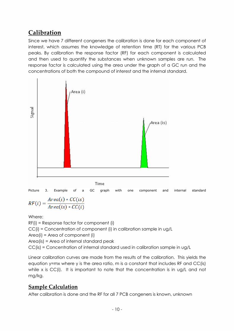
Calibration Since we have 7 different congeners the calibration is done for each component of interest, which assumes the knowledge of retention time (RT) for the various PCB peaks. By calibration the response factor (RF) for each component is calculated and then used to quantify the substances when unknown samples are run. The response factor is calculated using the area under the graph of a GC run and the concentrations of both the compound of interest and the internal standard.
Picture 3. Example of a GC graph with one component and internal standard
Where: RF(i) = Response factor for component (i) CC(i) = Concentration of component (i) in calibration sample in ug/L Area(i) = Area of component (i) Area(is) = Area of internal standard peak CC(is) = Concentration of internal standard used in calibration sample in ug/L
Linear calibration curves are made from the results of the calibration. This yields the equation y=mx where y is the area ratio, m is a constant that includes RF and CC(is) while x is CC(i). It is important to note that the concentration is in ug/L and not mg/kg.
Sample Calculation
After calibration is done and the RF for all 7 PCB congeners is known, unknown

- 11 -
sample runs can be quantified using:
Where: M(i) = The amount of component (i) present in the sample in mg/kg IS = The mass of internal standard added to the analysis samples in ug SA = The mass of sample material dissolved in solvent in g RF(i) = Response factor for component (i) calculated from the calibration run Area(i) = The area of component (i)’s peak in analysis RF(is) = Response factor of internal standard (which is 1 by definition) Area(is) = Area of internal standard peak in analysis
By using SA in the quantification phase the units are changed to the required format ug/g which is the same proportion as mg/kg. To complete the quantification and find 7PCB the 7 components, M(i), are summed.

- 12 -
Materials and Methods
Standards
Firstly, standards must be prepared in concentrations between 0.001 to 0.1ug/L, the internal standard concentration is made constant at 0.01ug/L. The chemicals needed for this procedure are as follows: PCB mix 3 in iso-octane (2,2,4 trimethylpentane) from Dr Ehrenstofer®, Germany, concentration is 10ng/uL of each of the 7 PCB congeners Internal Standard PCB 189 in iso-octane from Dr Ehrenstofer®, Germany, concentration is 10ng/uL Acetone from Merck® purity ≥ 99.0% Iso-octane from Merck® purity ≥ 99.5%
The equipment required are: 4dp analytical weighing scale from CSG®, UK Pipettes, plastic disposable 25ml Pyrex® flask, accuracy ±0.04ml 10ml Pyrex® flask, accuracy ±0.025ml Nitrile gloves
For calibration 10 standards were produced, but only 9 were used in the calibration due to contamination. The concentration of each standard was calculated using the equation below.
Where: m(mix3) = mass of PCB mix 3 (g) c(mix3) = concentration of mix 3 (ng/uL) m(189) = mass of internal standard added (g) c(189) = concentration of internal standard (ng/uL) m(tot) = m(mix3) + m(189) + mass of solvent (iso-octane) added (g) c(cong) = concentration of each of the 7 PCB congeners (ug/L) c(IS) = concentration of internal standard (ng/uL)
The c(cong) should be in the range of 0.1-0.001ug/L so this is kept in mind while adding solvent to the standard and the mass of solvent is varied to keep the standard within the concentration range. Since the concentration of the internal standard is constant, a specific volume of the internal standard was added; which had been calculated beforehand by using the density of the solvent.

- 13 -
Instrument Setup:
Carrier Gas: Helium, Yara Praxair, Köping, Sweden GC: Finnigan AQA® Trace GC 2000 Series, Thermo Quest®, Lund, Sweden Column: Rxi®-5Sil MS 30m , 0.25mm ID , 0,25µm film thickness, from Restek®, USA Pre-Column: Rxi® 5m pre column, Restek®, USA MS: Fison MD800, Thermo Quest®, Lund, Sweden AutoSampler: AS200, Thermo Quest®, Lund, Sweden
The GC inlet temperature is held at 230°C, injection was performed in splitless mode, carrier gas flow was kept at 1.6ml/min. The initial oven temperature is at 80°C for 1min, and then ramped with 20°C/min to 150°C, thereafter ramped with 5°C/min until temperature reaches 280°C, a final ramp with 50°C/min until 340°C and held for 10min. Total runtime is 43 min. The MS detector voltage is at 500V. SIM acquisition mode is used and the ions monitored are the M+, (M-Cl)+ and (M-2Cl)+ of each congener in their respective retention windows. MS acquisition begins 10 min after initial injection and is halted at 35 min. Each standard is run 3 times in a row starting with the lowest concentrations since high PCB concentrations also means a higher chance for PCB to stay in the column. Also pure iso-octane runs were done in between the different concentrations as a way to ensure no residue from the previous runs.
CB Structure Formula MW M+ (M-CL)+
(M-2Cl)+
28 2,4,4’ trichlorobiphenyl C12H7Cl3 257.55 256.54 221.09 185,64
30 2,4,6-Trichlorobiphenyl C12H7Cl3 257.55 256.54 221.09 185,64
31 2,4’,5 trichlorobiphenyl C12H7Cl3 257.55 256.54 221.09 185,64
52 2,2’,5,5’ tetrachlorobiphenyl C12H6Cl4 291.99 290.98 255,53 220,08
101 2,2’,4,5,5’ pentachlorobiphenyl
C12H5Cl5 326.44 325.43 289,98 254,53
118 2,3’,4,4’,5 pentachlorobiphenyl
C12H5Cl5 326.44 325.43 289,98 254,53
138 2,2’,3,4,4’,5’ hexachlorobiphenyl
C12H4Cl6 360.88 359.87 324,42 288,97
153 2,2’,4,4’,5,5’ hexachlorobiphenyl
C12H4Cl6 360.88 359.87 324,42 288,97
180 2,2’,3,4,4’,5,5’ heptachlorobiphenyl
C12H3Cl7 395.33 394,32 358,87 323,42
189 2,3,3’,4,4’,5,5' heptachlorobiphenyl
C12H3Cl7 395.33 394.32 358.87 323,42

- 14 -
209 Decachlorobiphenyl C12Cl10 498.66 497.65 462.20 426.75
Table 1: PCB congener nomenclature, formula molecular weight and monitored ions
Elution order and Retention Time:
To find elution order and retention time, standards were run containing all the components of interest. Runs were carried out in both full scan mode and SIM of all ions in table 1. Using Xcalibur® Qualitative Browser the different peaks were identified. Different temperature programs were initially tested and adjusted and finally the choice was made to use the one described above.
CB 28 52 101 118 153 138 180 189 (IS) RT
(min)
13.45 14.60 17.60 19.83 20.60 21.50 23.90 25.85
Table 2: Elution order and retention times of the 8 PCB congeners
Processing method:
Next step is to create a processing method in Xcalibur®, using all the data from above, to automate the procedure and print out reports for runs of unknown samples. For each component (congener), retention time and Interactive Chemical Information System (ICIS) peak detection algorithm were used as a basis for identification. A report was created that includes relevant information of the sample, a graph of the entire run and each PCB congener mass (see Typical Sample GC/MS PCB Report).
Sample preparation:
If sample preparation is done incorrectly or carelessly then any analysis performed is useless. It is of vital importance to prepare samples in a strictly disciplined and consistent manner. The sample preparation is a variation of the one found in SNV report number 4697 (Jansson B. 1997).
Instructions for preparation of soil samples for analysis:
Dry the earth for 2hrs in 60°C Weigh 1.5-2g earth in a test tube (note mass to 2 decimal places (dp) ) Add internal standard PCB189 to sample (note mass to 4dp) Add iso-octane and 3-4 drops of sulphuric acid and place in ultrasound water bath for 3hrs Wash with distilled water and extract the top solvent phase by pipette In the test tube there is now iso-octane + known mass of internal standard + extracted PCB from soil sample Wash again with 3ml sulphuric acid, wait up to 15 minutes for separation of acid and solvent to occur

- 15 -
If solvent is not clear or there is still debris in the solvent phase, extract the top phase and flush it through a florosil® (jtbaker) to remove excess debris The sample is then transferred to a 10 ml flask and iso-octane is added till the 10 ml mark The sample is taken from the 10 ml flask and transferred to an autosampler vial
Note: a blank sample is always prepared in conjunction with soil sample preparations. A blank sample is prepared in the same way as other samples and consists of iso-octane and internal standard only. All soil samples are run twice and the results are compared.

- 16 -
Results and Discussion
The method described above has been derived from many different attempts using different solvents, columns and temperature programs as well as fine-tuning the software. What has not been changed throughout is the way the soil samples were prepared and the standards were made for calibration. This part of the thesis will describe the process of how the final method was chosen, why it was chosen and results of analysis on soil with the final method.
The choices of solvent for the experiment were cyclohexane and iso-octane (specifically 2,2,4 trimethylpentane). Iso-octane was the main choice from literature concerning qualitative and quantitative analysis of PCBs [(Buthe & Denker, 1994);(Frame, 1997)]. Cyclohexane was used in one paper (Hong, A., 2008). Cyclohexane, due to its chemical structure (6 sided carbon circle), is a good solvent for PCB since they are similar in structure. Also, PCB mixtures with both cyclohexane and iso-octane as solvents were available and thus cyclohexane was also tested. The standard solutions were mixed from stock solutions of PCB congener mixtures from the chemical supplier Dr. Ehrenstofer. One used iso-octane as a solvent, was named “PCB mix3” and has 7 PCB congeners with concentrations of 10ug/mL. The second used cyclohexane as a solvent and was named “PCB mix21” and contains the same 7 PCB congeners plus CB31, also with each component concentration at 10ug/mL. The internal standard chemicals used were also from Dr. Ehrenstofer. One used iso-octane as a solvent and was called “CB189”. It contained only the congener 189 in concentration 10ug/mL. The other used cyclo-hexane as a solvent, was called “PCB mix26” and contained both CB30 and CB209 in concentrations of 10ug/mL. There was 2 choices of column that were available in the lab, a 5% dimethyl, 95% diphenyl polysiloxane 30m column which was already installed in the GC and a 5% methyl, 95% phenyl polysiloxane 30m column was also available.
Fullscan vs SIM
Using fullscan mode for detection of the PCB congeners in mix 3 yielded unusable results (see figure 1). 7 peaks were expected but instead there was a large broad peak and also many small peaks. Figure 2 was scanned using SIM mode which was much more promising as there were clear peaks and a relatively stable baseline. Column bleeding was evident in both as one can see how the baseline noise gets higher towards the end of the runs in figure 1 and 2. Since we require detection of low concentrations of PCB, SIM is the mode of detection that is much more precise and selective and will be the best choice for the method. The ions of each congener to be detected are [M]+, [M-Cl]+ and [M-2Cl]+.
Since the fullscan mode detects all mass sizes of ions from 100-500m/z and since there are many ions within the mass range, using SIM will probably yield more accurate results.

- 17 -
RT: 10,08 - 29,92
11 12 13 14 15 16 17 18 19 20 21 22 23 24 25 26 27 28 29
Time (min)
25
30
35
40
45
50
55
60
65
70
75
80
85
90
95
100
Re
lative
Ab
un
da
nce
13,20
10,68 13,71
13,1112,30
12,6811,87
11,72 29,5229,1527,7427,6511,09
27,45
27,3314,02
27,0514,12
26,91
26,7914,61
26,6715,1526,1925,37
25,2724,4815,3024,4215,68
23,6216,11
22,7221,74
23,5416,47 17,1820,70
19,6018,44 21,18
17,8719,15 20,59
NL:
8,80E5
TIC MS
stdms
Figure 1. Fullscan run of PCB mix3 , Temperature program (TP): initial temperature 65°C for 1 min, 10°C/min
to 300°C held for 2 min, 50°C/min to 315 held for 9 min.
RT: 20,02 - 29,96
20,5 21,0 21,5 22,0 22,5 23,0 23,5 24,0 24,5 25,0 25,5 26,0 26,5 27,0 27,5 28,0 28,5 29,0 29,5
Time (min)
25
30
35
40
45
50
55
60
65
70
75
80
85
90
95
100
Re
lative
Ab
un
da
nce
22,01
21,7622,73
20,7129,60
29,4428,41 29,1328,2527,6923,64 27,54
27,3527,14
24,4926,89
25,40 26,7524,96 26,2825,52
24,2924,19
23,5223,0222,11
20,90 21,4320,34
NL:
1,74E6
TIC MS
std_10032
3013911si
m
Figure 2. SIM run of PCB mix3, same TP as Figure 1.
Column change
Running tests on the 5%diphenyl, 95%dimethyl siloxane column it was very difficult to get clear readings. Even after running only solvents overnight at high temperatures, high mass ions were found, which may be due to contaminants that were trapped in the column. Both cyclohexane and iso-octane PCB mixture standards were run using SIM yielding many ghost peaks and uneven baselines. The temperature program used was: initial temperature 65°C for 1 min, ramped at 10°C/min until 300°C and held for 2 min, ramped again at 50°C/min until 315°C and held for 9min. The cleaning temperature program: initial temperature 65°C for 1 min, ramped at

- 18 -
40°C/min until 250°C and held for 2 min, ramped again at 30°C/min until 320°C and held for 8min.
RT: 5,05 - 17,91
6 7 8 9 10 11 12 13 14 15 16 17
Time (min)
40
45
50
55
60
65
70
75
80
85
90
95
100
Re
lative
Ab
un
da
nce
6,166,14
6,26
6,33
6,07
6,00 6,46
5,946,58
6,64
6,77
5,62 6,94
10,5911,06
7,129,94
12,3210,157,2911,66
11,70 17,727,35 9,74 17,6313,087,729,26 17,0214,3412,21 12,43 14,118,05 15,5914,42 16,1213,218,70
8,159,06 9,66
NL:
8,96E5
TIC MS
cleaningwit
hiso
Figure 3a. SIM run of pure iso-octane solvent, new TP for column cleaning: init temp 65°C for 1 min, 40°C/min
to 320°C held for 10 min
RT: 5,01 - 17,92
6 7 8 9 10 11 12 13 14 15 16 17
Time (min)
25
30
35
40
45
50
55
60
65
70
75
80
85
90
95
100
Re
lative
Ab
un
da
nce
5,24
5,68
5,62
6,14
5,78
6,65
6,3410,59
9,26 9,748,70 10,1611,057,29 8,05
11,67 12,3115,286,70 15,58 17,1015,20 15,97 17,5216,3514,6714,0513,0712,25 12,3911,14 13,13
7,71 9,318,778,47
NL:
1,25E6
TIC MS
cleaningwit
hcyclo_100
316092750
Figure 3b. SIM run of pure cyclohexane, same TP as 3a
Many pure iso-octane and cyclohexane runs were performed as a way to purge contaminants from the column (figure 3a and 3b). As it appears there are many peaks with ion masses that correspond to PCB congeners, however, since there are so many peaks and the specific ions that are monitored are chosen by the operator, it is impossible to specify with certainty what these ions can be. What can be said is that they are interfering with the analysis. After running 10 cleaning cycles with both iso-octane and cyclohexane, another standard run is performed (see figure 4).

- 19 -
RT: 7,03 - 34,91
8 9 10 11 12 13 14 15 16 17 18 19 20 21 22 23 24 25 26 27 28 29 30 31 32 33 34
Time (min)
25
30
35
40
45
50
55
60
65
70
75
80
85
90
95
100
Re
lative
Ab
un
da
nce
14,76
16,27
17,65
13,07
14,10
18,90
31,51
20,05 21,15
22,1727,81 31,14 31,7323,13 27,6624,0211,11 24,88
28,8925,87
34,1330,18 31,9433,68
30,0617,1315,34
8,938,81 19,1112,93 18,7510,929,787,72
NL:
1,22E6
TIC MS
standard2
Figure 4. SIM run of [PCB Mix21]=0.1091 in cyclohexane, TP: init temp 65°C for 1 min, 10°C/min to 300°C
held for 2 min, 50°C/min to 315 held for 9 min
It is very difficult to look for specific PCB congener peaks in this chromatogram. Many chromatogram peaks contain a large amount of mass peak 220/221. Peaks are spaced in what looks like regular intervals and it seems more and more likely that the column is not in good condition. There are too many peaks to find anything of value so a decision to run analysis on a standard containing only PCB congener 189 in order to at least find one good peak was made (figure 5). The 2 main peaks in this run were found at 20.95 min and 21.96 min, both contained ion mass 396, CB189s largest ion is 394.32. At this stage there was only one thing left to do, that is, change the column.
RT: 19,96 - 34,87
20 21 22 23 24 25 26 27 28 29 30 31 32 33 34
Time (min)
10
15
20
25
30
35
40
45
50
55
60
65
70
75
80
85
90
95
100
Re
lative
Ab
un
da
nce
20,95
21,96
34,7433,7433,4532,9031,01 31,8430,9029,5628,34 29,3527,6627,4927,1022,70 23,6121,73 25,35 26,4624,4420,68
NL:
4,61E6
TIC MS
0p1072
Figure 5. SIM run of internal standard [CB189]=0.1183 in iso-octane, same TP as Figure 4

- 20 -
New column runs and choice between iso-octane and cyclohexane as
solvent
The temperature program used was: initial temperature 80°C for 1 min, ramped at 5°C/min until 300°C and held for 2 min, ramped again at 50°C/min until 315°C and held for 9 min. The ramp was reduced from 10°C/min to 5°C/min in order to gain better resolution at the expense of longer run time.
RT: 20,02 - 34,99
21 22 23 24 25 26 27 28 29 30 31 32 33 34
Time (min)
25
30
35
40
45
50
55
60
65
70
75
80
85
90
95
100
Re
lative
Ab
un
da
nce
24,58
22,70
23,29
21,65
20,6721,85 23,7421,20 23,89 25,19
26,11 30,9027,20 33,0828,6027,4627,07 30,1728,75 31,7529,71 33,7231,84 34,9334,35
NL:
2,75E6
TIC MS iso
Figure 6. SIM run of the solvent iso-octane, TP: init temp 80°C for 1 min, 5°C/min to 300°C held for 2 min,
50°C/min to 315°C held for 9 min
Iso-octane solvent run shows 4 ghost peaks with mass peak 220/221 being the largest peak.
RT: 20,05 - 34,99
21 22 23 24 25 26 27 28 29 30 31 32 33 34
Time (min)
20
30
40
50
60
70
80
90
100
110
Re
lative
Ab
un
da
nce
33,72
34,9323,3532,95
29,65 30,5628,8426,59
21,9920,41 21,87 22,19 33,0723,47 24,86 33,8330,8926,08 27,60 28,6025,04 30,1726,71 28,95 31,32 32,66
NL:
2,41E6
TIC MS
0p0176
Figure 7. SIM run of [PCB Mix3]=0.1072, high concentration, same TP as figure 6

- 21 -
RT: 20,05 - 34,99
21 22 23 24 25 26 27 28 29 30 31 32 33 34
Time (min)
20
30
40
50
60
70
80
90
100
Re
lative
Ab
un
da
nce
34,93
23,3532,95
29,6530,56
28,84
26,59
21,99
20,43 33,0720,77 30,8922,17 22,68 26,1324,8623,64 28,60 33,7225,62 27,6227,04 28,96 30,17 32,5131,42
NL:
3,42E6
TIC MS
0p1072
Figure 8. SIM run of [PCB Mix3]=0.0176, medium concentration, same TP as figure 6
Comparing figure 7 and 8 one can finally see that they have 7 peaks in common which is a very positive result. Also the ghost peaks in the iso-octane run (figure 6) disappear since they are very small compared to the analyte peaks. This is a step forward towards a successful calibration of the instrument. At 33.72 min there is a ghost peak with mass 220/221. This is a recurring ion mass that has been present even with the old column. Since the column has been changed the reason for the ghost peak with mass 220/221 must be due to a different cause, possibly the MS.
RT: 20,01 - 34,99
21 22 23 24 25 26 27 28 29 30 31 32 33 34
Time (min)
80
82
84
86
88
90
92
94
96
98
100
Re
lative
Ab
un
da
nce
23,35
32,9534,93
20,4329,65
30,5628,8426,59
33,07
21,9920,76
22,6821,8430,89
26,1023,53 24,25 24,87
28,6025,61 27,63
26,77 30,17 33,7128,25
28,9831,13 31,86 32,47 33,89
NL:
7,66E5
TIC MS
0p0048
Figure 9. SIM run of [PCB Mix3]=0.0048, low concentration, same TP as figure 6
Whenever concentrations lower than 0.01ug/mL are analysed, the baseline is raised heavily and a lot of noise is present (figure 9). This will make it very difficult to be accurate under 0.01ug/mL which is what is required of the method. This noise must be coming from the MS itself and since it has been out of use for a period of time, degradation of the electronics and/or ion source could be the cause.
As the 7 PCB congener peak were successfully found in iso-octane, cyclohexane standards were prepared and run, cyclo-hexane mix 21 has 8 PCB congeners.

- 22 -
RT: 20,00 - 50,00
20 22 24 26 28 30 32 34 36 38 40 42 44 46 48 50
Time (min)
55
60
65
70
75
80
85
90
95
100
Re
lative
Ab
un
da
nce
48,00
25,80 37,68
46,5927,70
48,1624,00
45,7025,95 45,5323,19 25,6123,0321,60
28,53 44,8928,82 30,08 41,8731,52 44,5935,7834,55 36,22 41,6439,06
NL:
7,49E5
TIC MS
0p0062
Figure 10. SIM run of [PCB Mix21]=0.0062 , low concentration, same TP as figure 6
Low concentration of analyte yielded yet again high baseline and noise (figure 10).
RT: 20,00 - 50,00
20 22 24 26 28 30 32 34 36 38 40 42 44 46 48 50
Time (min)
10
20
30
40
50
60
70
80
90
100
Re
lative
Ab
un
da
nce
48,02
25,80
27,69
46,5941,86
28,52 47,8024,00 37,6735,78 45,0844,5926,64 38,93 48,8328,7723,5921,85 43,0140,2430,50 35,4433,93
NL:
1,43E7
TIC MS
cyclo1
Figure 11. SIM run of pure cyclohexane, SIM, same TP as figure 6
Comparison of the pure cyclohexane run (figure 11) and a run using PCB mix21 as a sample (figure 10), shows that all the peaks in the sample run are also in the solvent run and therefore no PCB congener peaks are detected at the low concentration 0.0062ug/mL.
RT: 20,00 - 50,00
20 22 24 26 28 30 32 34 36 38 40 42 44 46 48 50
Time (min)
0
10
20
30
40
50
60
70
80
90
100
Re
lative
Ab
un
da
nce
25,94
48,00
27,31
25,80 33,6134,52
27,69 46,5930,55
32,81 36,9225,6024,00 41,8537,6628,51 45,0835,77 48,5444,9123,60 38,9228,7721,85 41,2831,88
NL:
6,13E6
TIC MS
0p1091
Figure 12. SIM run of [PCB Mix21]=0.1091, high concentration, same TP as figure 6

- 23 -
With higher concentration of the PCB congeners, several peaks are found. The pure solvent run (figure 11) shows that there are certain ghost peaks though. Use of a background subtraction is therefore done to get a clearer picture.
RT: 25,38 - 37,22
26 27 28 29 30 31 32 33 34 35 36 37
Time (min)
0
10
20
30
40
50
60
70
80
90
100
Re
lative
Ab
un
da
nce
25,94
27,31
33,6134,52
30,5532,81 36,92
33,3831,88 34,6934,32 36,6330,67 35,14 35,6830,1329,83 32,5627,8926,02 31,1928,26 29,3826,67
NL:
5,50E6
TIC MS
BG_0p109
1
Figure 13. [Mix 21]=0.1091 Background subtracted with solvent run
As seen in figure 13, there are 7 peaks that may correspond to the different congeners in solution. The peak at 25.94 minutes is very large and a simple explanation could be that this is actually 2 peaks. Both CB21 and CB30 are eluting here due to their close similarities in structure and formula.
The retention times (RT) of the different congeners are found, using qualitative analysis the order of elution has also been established:
Elution order
(CB)
RT GCMS (min)
PCB mix3
RT GCMS (min)
PCB mix21
28 23.35 25.94 (also CB31)
52 26.59 27.31
101 28.84 30.55
118 29.65 32.81
153 30.57 33.61
138 32.96 34.52
180 34.94 36.92 Table 3. Elution order and RT for PCB congeners in both cyclohexane (PCB mix21) and iso-octane (PCB mix3).
Looking at the figures in this section using iso-octane as a solvent seems to be the best choice, there are several reasons for this. There were many unknown ghost peaks in cyclohexane that disrupt analysis. The congeners 28 and 31 were not easy to separate; congener 31 is also not part of the 7PCB sum used by SNV for PCB quantification. Running low concentrations with cyclohexane yielded little/no usable peaks (see figure 10) while with even lower concentration of PCB mix3 in iso-octane (figure 9) showed much clearer peaks. So, even though cyclohexane has a similar structure to PCB and is therefore a good solvent, the results yielded in

- 24 -
comparison to iso-octane are inferior. Since the MS already has a high baseline and a lot of noise when running low concentrations the choice of solvent for this method is iso-octane.
Internal Standard RT
Following the choice made to use iso-octane as a solvent the chemical used for the internal standard (IS) used will be the congener CB189 in iso-octane. This congener is not naturally formed when producing industrial PCB mixtures and was therefore a prime candidate for use as an internal standard. Analysis of sample containing only CB189 in iso-octane using the same temperature program revealed its retention time at approximately 35min. We can see from table 3 that the RT is very close to CB180, which may be a problem if they are not sufficiently separated. Next step is to fine-tune the temperature programming and run standards that contain the 7PCB congeners and the internal standard CB189 to get new RT and start the calibration process.
Calibration and Process method 1
The temperature program that was used was: init temp 80°C for 1 min, ramped with 5°C/min until 280°C and held for 1 min, ramped again with 50°C/min until 320°C and held for 10min. This temperature program was used in figures 14-16. RT: 20,00 - 35,00
20 21 22 23 24 25 26 27 28 29 30 31 32 33 34 35
Time (min)
0
10
20
30
40
50
60
70
80
90
100
Re
lative
Ab
un
da
nce
24,57
21,65
23,29
22,69
23,7526,60 32,9629,65 30,5728,86 34,9421,99 25,2023,8920,75 26,11 27,06 30,8828,59 32,59 33,06
NL:
8,58E6
TIC MS
0p0093
Figure 14a. SIM run of [PCB mix3]=0.0093 + internal standard [CB189]=0.01
RT: 20,03 - 35,00
21 22 23 24 25 26 27 28 29 30 31 32 33 34 35
Time (min)
8
9
10
11
12
13
14
15
16
Re
lative
Ab
un
da
nce
24,5721,65 23,2922,69
23,75
26,60 32,96
29,65 30,5728,86
34,94
21,99
25,2023,8920,75
26,1130,32
27,0625,56 27,4521,20 29,11 30,8820,42 28,59
32,59 33,0633,7231,78
34,12
NL:
8,58E6
TIC MS
0p0093
Figure 14b. Zooming in by baseline

- 25 -
RT: 20,00 - 35,00
20 21 22 23 24 25 26 27 28 29 30 31 32 33 34 35
Time (min)
0
10
20
30
40
50
60
70
80
90
100
Re
lative
Ab
un
da
nce
24,59
32,9723,36
26,60 29,6621,66 28,87 30,5923,30
22,71
23,75 34,9625,2020,77 27,8025,32 30,3327,06 29,11 33,7228,42 30,88 32,6031,81
NL:
1,93E7
TIC MS
0p0966
Figure 15. SIM run of [PCB mix3]=0.0966 + internal standard [CB189]=0.01
Studying figures 14 and 15, 7 PCB peaks and the internal standard at 34.95 min can be seen and are detectable so retention times are established. Next step is to create a process method that will quantify those peaks. However, there were also 4 ghost peaks between 21-25min that contain a peak ion with mass 220/221. This reoccurring ion must be a contaminant from somewhere in the system. Also the noise level is quite large for the lower concentration and this will definitely cause quantification to be highly inaccurate at these low concentrations.
CB 28 52 101 118 153 138 180 189 Average RT (min) 22.00 23.36 26.59 28.85 29.65 30.57 32.95 34.94 Table 2. Elution order and average RT for calibration 1
There were 5 standards prepared and each one was run 3 times thus calculating an average with 15 values of RT for each congener. Subsequent runs without ion 220/221 in SIM mode (figure 16) yielded much better separation and can be used for quantitative analysis. The large ghost peak at 24.6 min was reduced without 220/221 in SIM (compare figure 15 and 16).
RT: 20,00 - 35,00
20 21 22 23 24 25 26 27 28 29 30 31 32 33 34 35
Time (min)
0
10
20
30
40
50
60
70
80
90
100
Re
lative
Ab
un
da
nce
32,95
28,8626,60
29,65 30,57
23,36
24,5821,99
22,69
23,7534,94
25,1923,8921,6620,76 30,3227,7825,32 33,7029,1128,4127,39 30,88 32,5931,81 33,84
NL:
4,65E6
TIC MS
0p0966
Figure 16. SIM run of [PCB mix3]=0.0966 + internal standard [CB189]=0.01, SIM mode edited to exclude ion
mass 220/221

- 26 -
The process method was developed using a linear calibration curve with ug/L as units, 5 calibration levels at 1 , 4 , 9 , 50 and 97ug/L were used. Identification of peaks used an ICIS algorithm and the retention times of said peaks. MS acquisition using SIM of 30 ions was utilized. The results of the process method showed good linear fit for all the congeners (R2>0.99 for all components/congeners), however, for low concentrations the percentage difference between expected and calculated amounts was much too large (see graph 1) to give good results for the method being developed. One main reason for this is the high noise level which is most probably due to a problem with the hardware in the MS and the solution to this is for a technician to service the instrument. Another way to improve the detection and lower the difference is to limit the SIM to look for fewer ions during retention windows that correspond to the different congeners. By looking for three main ions of each congener in its respective retention window the MS is much more specific and will give more accurate results as it can read more data points/sec when searching for 3 ions instead of 30.
Graph 1. Relative difference between actual and expected values for the congeners with concentration at
0.0007ug/ml
Calibration and Process method 2
The changes that were made: instrument technician took apart and cleaned the MS. A 5 meter precolumn guard was connected to the 30meter GC column (this causes the RT for all the congeners to change). MS acquisition in SIM mode was changed to detect 3 ions in specific retention windows, the TP was changed by adding another ramp to reduce run time, 9 completely new standards were made for the calibration and the results were much more accurate than before (see figure 17). There is still noise when dealing with low concentrations (see figure 18) though, and further investigation performed by the instrument technician showed a possible electrical problem; which caused a very uneven baseline. Also there seems to still be ghost peaks, however, they are not as large as before and also do not influence

- 27 -
the quantitative aspect either as the ghost peaks are not close to the PCB peaks. There is good selectivity between the components in this method (figure 17).
RT: 13,00 - 26,00
13 14 15 16 17 18 19 20 21 22 23 24 25 26
Time (min)
15
20
25
30
35
40
45
50
55
60
65
70
75
80
85
90
95
100
Re
lative
Ab
un
da
nce
14,6213,44
20,60
21,52
19,83
17,63
14,39
23,88
20,9013,93
25,8614,72 17,76 18,16 19,9219,74 21,23 21,64 22,03 24,2022,65 24,90 25,4423,48
NL:
5,82E5
TIC MS 2
Figure 17. SIM run of [PCB mix3]=0.0499 + internal standard [CB189]=0.009, TP: init temp 80°C held 1 min,
20°C/min to 150°C, 5°C/min to 280°C, 50°C/min to 340°C held 10min
RT: 12,93 - 26,29
13 14 15 16 17 18 19 20 21 22 23 24 25 26
Time (min)
60
62
64
66
68
70
72
74
76
78
80
82
84
86
88
90
92
94
96
98
100
Re
lative
Ab
un
da
nce
13,46
14,64
13,73
13,95 25,8813,24
20,6214,77 17,65
14,41 19,8514,9221,5319,84
19,7117,7919,92
20,1020,94 23,89
21,83 24,0321,93
24,83 25,3324,2123,1122,87 23,44 25,50
NL:
1,04E5
TIC MS 5
Figure 18. SIM run of [PCB mix3]=0.0007 + internal standard [189]=0.009, same TP as figure 17
The new process method used a linear calibration curve with ug/L as units. 9 calibration levels at 0.7, 1 , 4 , 8 , 9 , 10 , 49, 50 and 97ug/L were used. Identification of peaks used an ICIS algorithm and the retention times of said peaks. MS acquisition used SIM mode of 3 ions for each congener in its respective retention window, this also increased detection capabilities of the MS since it was searching for fewer ions per unit of time. The results of this new process method also shows an acceptable linear fit for all the congeners (R2>0.96 for all components/congeners [see table 4]), and the percentage differences between expected and calculated amounts for concentrations under 1ug/L was up to 100%, while standards between

- 28 -
4-10ug/L deviated up to 15% (see graph 2). Under the circumstances these results are adequate and can be used for calibration and soil sample analysis.
Graph 2. %difference vs Calibration concentration in ug/L of all the 7 PCB congeners
Each of the standards was run 3 times and the precision of the tests were very high, however it seems that accuracy was lacking in tests under 1ug/L. It looks like there could have been a possible miscalculation or preparation error with the standard at 49.9ug/L as the higher and lower concentrations both have much smaller error range. When the same standards were run 3 times the results of each run was very similar to each other with plus minus 5% difference.
Congener 28 52 101 118 153 138 180 R^2 0.9696 0.9689 0.9724 0.9699 0.9710 0.9732 0.9688 Table 4. Correlation coefficients of the linear calibration curves for each component/congener
Soil Samples and Reports
Unknown soil samples were analyzed using the GC/MS, the development of automated reports for the analysis of soil samples was done using a template in Word and with the user manual for Xcalibur®. The report mirrored reports done previously by LjungaLab and thus included a graph of the run, sample weight, a breakdown of the 7 PCB congener masses and their retention times. The operator must manually add the 7 peaks and divide by sample weight to get the final result in

- 29 -
mg/kg. The reports are automatically printed (see below for example) after each sample run allowing for overnight/unsupervised runs
Typical Sample GC/MS PCB Report
Qualitative Peaks RT: 13.00 - 27.00 SM: 7G
13 14 15 16 17 18 19 20 21 22 23 24 25 26 27
Time (min)
55
60
65
70
75
80
85
90
95
100
Rela
tive A
bundance
25.94
14.4620.96
13.50
19.6017.17
15.34 21.87
24.08 24.8723.05
NL:
6.36E4
TIC MS
9882-1
Sample Name: xxxx-xx
Sample Type: Unknown
Date: 06/15/2010 10:15:14 PM
Data Path: C:\xx\yy\
Samp Wt (g): 0.58
Istd Amt (ng): 44.000
Inst Method: C:\PCB\Methods\xxx
Proc Method: C:\PCB\Methods\yyy
Name Actual RT (min) Calculated Amount (ng)
IS189 25.94 0.000
28 13.50 0.765
52 14.69 0.078
101 17.73 0.127
118 19.92 0.036
138 21.60 0.209
153 20.67 0.683
180 23.97 0.079
Sum Calculated Amount : _____1.977__________ ng
7PCB = Sum Calculated Amount (ng) / ( Samp Wt (g) * 1000 ) = _____0.003__________ mg/kg

- 30 -
Pedagogics
Theoretical Framework
Throughout history there have been many theories of what learning and knowledge are and how they are achieved. The source theories that I have decided to use and will describe below are Vygostkijs sociocultural theory, Piagets cognitivism and Mezirows Transformative and Emancipatory Learning. Both Vygotskij and Piagets theories are developed from the earlier cognitivistic theories of learning, which is described by Imsen as learning is an independent inner process (Imsen 2000).
Transformative and Emancipatory Learning
Fostering Critical Reflection in Adulthood by Mezirow coins the term transformative learning which is an adult form of metacognitive reasoning, i.e. how adults learn and know. It “can take place without professional interventions and within an educational context” and the goal of an adult educator is to get them to that stage through the use of communication. “Learning is grounded in human communication”.
Transformative learning is the process of learning through critical self reflection to allow an integrative understanding of the learning experience. In layman terms the goal of transformative learning is for the student to become proficient enough so that he or she can use the knowledge and information, and without further guidance act upon it and begin to use it in new and inventive ways. According to Mezirow “Rational thought and action are the cardinal goals of adult education”. For example attending a course without later practicing what was learned is a waste of time. Rational thought, critical reflection and reasoning must take place for benefit to be gained and transformative learning to be accomplished.
Mezirow states that “to make meaning means to make sense of an experience” and when we interpret the experience to guide decision then “meaning becomes learning”. He argues that “we learn differently when we are learning to perform than when we are learning to understand what is being communicated to us”. Mezirow also describes reflection as “enabling us to correct distortions in our beliefs and errors in problem solving.” while critical reflection “involves a critique of the presuppositions on which our beliefs have been built.” Mezirow concludes by writing “Learning is not a desirable outcome or a goal; it is the activity of making an interpretation that subsequently guides decision and action. Learning is grounded in the very nature of human communication.” (Mezirow 1990)
Social Constructivism
Social constructivism emphasizes the act of communication in a social context as the key to learning and understanding. The central aspects of social constructivism, according to Dysthe, is that the learning be: “situated, social, distributed and mediated”, also that “language is fundamental in the process of learning as well as

- 31 -
the teaching is inclusive of a group” (Dysthe 2003). Learning must take place in specific physical and social context (situated). If there is to be learning then there needs to be interaction between people (social). Certain people are more knowledgeable than others in certain areas, thus the combined knowledge of those people are required to gain a broad understanding and learning can take place between those people. With mediated Dysthe explains that tools and aids (or artefacts) for teaching are used to allow for a greater learning. The main theme is communication and its various forms, the correct lingo/language must be used, understanding the social and cultural environment is of great importance when coming from the outside to being able to teach.
Cognitivism
Piaget studied history and philosophy and his main interest was trying to figure out how knowledge is created, his theories were on where knowledge came from and how it developed. To test these theories, he studied children. Piaget believed that knowledge was created within the subject and the outside world provides a landscape in which one discovers and understands. It is a rationalistic perspective on human thought and communication. According to Säljö, Piagets metaphoric on how to create knowledge include “being active, finding things out on your own, laborative working and guided by curiosity”. The likeness to social constructivistic perspective is the strong emphasis Piaget has on learning by activity. The difference is that learning is an individual process and not a social one. (Säljö 2000)
Method Framework
This paper uses qualitative research as the company itself is very small (<4 employed) and the frame/scope is limited to a specific combination of machines and laboratory environment. The user manual created is for a specific model of analytical equipment and its software.
Introduction I spent the first part of my time at the company as a student in chemical engineering and not a teacher. The first week I worked with them at the laboratory, in the beginning I shadowed them, after that I helped out in each of their different topics of work, they don’t all do the same analysis and the analysis jobs vary largely both by shape and method. By the end, I developed a friendship with them, I learnt about them and what they do, I got a feeling for their way of life and lived in their environment and also got a sense for their personal styles. It is said as a teacher one must be objective and an observer but this could not be farther than the truth for me since before I could teach them how to do the analysis I had to develop the method, test it, reevaluate it and only thereafter could teach the staff how to perform the method. In my case I feel this was a strength since I became part of the team and afterwards I could step back, use the impressions made by them and the sociocultural environment to my advantage when teaching. In this section pedagogical theories are used to educate the staff. The

- 32 -
development of the user manuals have been done in conjunction with the staff to create a user manual that is tailored specifically for their use.
Method
Method Walkthrough: I settled on creating a User Manual to guide them through the methods of analysis and maintenance and developed worksheets to test their understanding and the readability of my user manual. Their input was noted, considered and used to update the manual to create a personalized version for the staff.
The Practical Problem
What needs to be taught to the next operator so that the method developed can be used and automation can be implemented? The software needs to be familiar; in this case we have Tune® and Xcalibur® as the software that needs to be understood on a basic level to be able to continue running tests and for general problem solving to be accomplished. The hardware that needs to be familiar is the GC and MS and the connection between the two. The Autosampler is the third piece of hardware that also needs to be taught as without it no automation can be achieved. What knowledge does the staff possess already? There is, for example, no need for me to teach the sample/standard preparation or how the GC works and is maintained as the staff have far superior knowledge and experience with it than I do. It is also worthy to note that the staff have a lot more experience and wisdom when dealing with safety in the lab, reading spectrum, analyzing spectrum and general lab maintenance.
Observation and Assessment In pedagogics, observation is being active and concentrating to be able to see things that have pedagogical relevance. True observation is hard to accomplish since we are bombarded with millions of impressions every second of every day. We cannot actually process all this information and thus filter out a very large part of all these impressions and, Nørretranders states that we consciously register 40 of the 11 million impressions received every second (Nørretranders 1992). So with this in mind it is very easy to imagine that different people can experience the same situation very differently. A model described in the book “Det värderande ögat” (Björndal 2002) helps us understand the way we take in and process information in a more visual way.

- 33 -
Figure A.1 Truth, perception and memory
The millions of stimulus enter our sensory memory for a short period of time and it is here the filter takes place, then we actually begin perceiving and building things that are meaningful to us, here is where different people will perceive different things. This is done in a subconscious state, our brain sees certain things and disregards others (also shown by the reduction in arrows from one state to another). From this stage the perception enters our short term memory, George A. Miller, a memory researcher, found that the short term memory has a finite capacity and can remember 7 units at a time (Miller 1956). For the final process of storing information in the long term memory, the information needs to be actively processed into abstract outlines, visual representations or verbally phrased. There is of course also some maintenance needed to keep the information in the long term memory, by actively recollecting events and or writing them down.
Transfer of knowledge The knowledge to be transferred can be broken down into different sections and these sections can then be made into step by step instructions and be placed in a user manual. According to Birget Lendahls there are different paths to learning, learn by watching, learn by doing and learn by reading (Lendahls 2005). I have used all three in teaching the staff to continue usage of the method and allowing them to run analysis of soil samples to detect low quantities of PCB. The sections are hardware maintenance (specifically GC and MS maintenance), autosampler setup, using the software Tune® to check for problems in the MS and Xcalibur® for recalibration and for analysis of unknown samples. 2 user manuals are produced, the first specifically deals with hardware maintenance and the second encompasses how to use the software and the autosampler setup. The reason for 2 separate manuals is that sample analysis is done much more frequently than the maintenance.
I used their coffee room as a gathering place for my introduction. I gathered the staff and handed out a printout of the user manual which we went through together. I gave a presentation on what I was going to teach them and then asked them to go through the user manual by themselves and put question marks and comments on things that are unclear. After gathering the manuals I rewrote and

- 34 -
improved it. A couple of days later I began 30minute a day lessons showing them how to use Tune®, Xcalibur® and the autosampler with the computer. While practically showing them how to use the programs and autosampler, they had the new revised user manual and I actively asked questions about what I was doing to make sure they were following. After the presentations were completed I took them independently and asked them to complete 2 worksheets which tested their ability to work independently. I observed this process and wrote down notes and used the experience as feedback which helped me further clarify and format the final draft of the user manual. The user manual was written in Swedish and on the next page is a translated outline of the user manuals.

- 35 -
Outline of User Manuals Chapters of the user manuals in English:
Hardware maintenance: Tune (weekly)
• Auto Tune and Auto Calibration (once a week) • Leak Checking • Supplementary information
GC
• Leak Check/Column Evaluation
MS
• Vacuum pump (weekly) • Source cleaning (every 3rd month) • Column Installation to MS
PCB Analysis: Xcalibur
• Calibration of GC/MS • Running unknown samples
o Sequence o Status and Acquisition Queue o 8 PCB congener retention times o Reports
• Processing Setup o Quantitative
� Identification/RT of components � Addition of new levels/changing ISTD concentration
o Reports
Autosampler AS800
Autosampler example

- 36 -
Results
Note that the results from my presentations as well as staff input were used directly to update the user manual since it is the main tool the staff can use to learn how to operate the machine as well as develop new methods from it. Below I describe the tasks of the worksheets and my raw observations as well as ideas for improvement to the user manual5.
Unknown Sample runs - Worksheet 1
In this worksheet6 the lab has received 8 samples that need to be tested for PCB. The sample preparation has been done and 8 sample vials are given to the operator. The test here is for the operator to correctly input the samples into a sequence using Xcalibur and to put the sample vials in the autosampler and program the autosampler to be in tune with the sequence so testing can be accomplished.
Reflections from Adam: Adam is an older gentleman in his 50’s who upon sitting at the computer to begin creating a sequence, begins directly asking lots of questions which I answer with “use the manual”. He types using 1 hand and very slowly, seems very unsure of the program which is understandable as this is his first time using the program. After writing up 3 of the 8 samples in sequence he begins to work independently, making his own observations about the program and talking while working, changing file names to suit himself which is fine to do as file names do not change the outcome of the test. *Improvement* I can tell that I need to add slides for status and acquisition queue as these were not discussed in the user manual. As Adam finished writing up the sequence I ask him to complete the autotune setup and to make sure both the autotune and sequence are in sync. He seems to have little problem in using the autosampler and uses the example in the user manual for the first few samples and completed the programming without.
Reflections from Eve Eve is in her 40’s and is very experienced in running PCB analysis. Upon seeing the program Xcalibur she sets straight to work using the manual to navigate into the sequence setup. She seems content with using the manual to work through the test and does so while singing. She completes the sequence training independently and begins working on the autosampler. Here problems occurred and she did not seem to understand how to use the example in the manual to help her program the autosampler. I aided her by doing a couple of samples for her and she was able to
5 See Appendix 1.1 and 1.2 for User Manuals 6 See Appendix 1.3 for worksheet

- 37 -
complete it. *Improvement* She told me that the first part of the example in the user manual was not clear and required clarification.
Calibration and process method modifications - Worksheet 2
In this worksheet7 the operator is taking the role of calibration of the GC/MS using Xcalibur. The new calibration is to be done with 4 standards which are given in vials to the operator. What is required is that the operator creates a new sequence for calibration, corrects the process method and makes sure the autosampler is ready and synchronized with the new sequence.
Reflections from Adam Adam was very unsure how to begin with the sequence, after some careful consideration it was underway. However, he seemed to have problems in adding the correct levels. *improvement* Clarification required in the “Level” chapter of the user manual. In the process method Adam was able to find and edit the correct areas but to accomplish it had to refer back to the user manual many times. This is not a bad thing as the user manual is there to be used and referred to when needed.
Reflections from Eve The sequence was created speedily and correctly; she seems to have understood and is able to use the information given at the lecture well. She had a bit of problems finding the actual process method but when found had no problem with editing it to suit the new calibration. *improvement* Make how to find the process method simpler. When moving to autosampler programming I noticed that Eve still was still unsure how to program it and was worried that she’d make a mistake. I believe that to get over the worry and insecurity of using the autosampler it is important to keep practicing with new questions to help solidify the understanding. She asked me to help and I did. After she was done I asked her to do another autosampler program with a sequence that I loaded at random. She was able to complete it at a better pace. However, it is obvious that more practice is needed in order to be secure in its usage. I inquired if there can be any improvements made for the autosampler section in the user manual but she said it felt like she could follow it and that it was good.
7 See Appendix 1.4 for worksheet

- 38 -
Analysis and Discussion
Summarizing the pedagogical aim, I set out to teach the staff how to run and maintain instruments using a few pedagogical theories such as Vygotskijs social constructivistic theory of learning, Piagets cognitivism and Mezirows transformative and Emancipatory education. My role as an educator is to teach the staff how to use and maintain the instruments and produce a user manual that will aid in independent analysis, the final goal being to achieve transformative learning (also called critical reflection) which would allow the staff to produce new methods for detecting and quantifying other chemical molecules using the same instruments (GC/MS).
With focus on the social constructivistic theories of learning, Dysthe breaks down the central aspects of learning into six parts: "situated, social, distributed, mediated, language is fundamental in the process of learning and the teaching is inclusive of a group” (Dysthe 2007). The learning is situated in that the teaching took place primarily in 2 physical areas, the coffee room and the analysis laboratory where the GC/MS machines were. The presentations and Q&A was performed in the coffee room and the worksheets were done in the analysis laboratory. The learning is social as we have discussed the user manual and aspects of the machines as well as done quite a bit of problem solving (during the method development phase of my thesis). Socially I had assimilated myself into their group as I had worked with them for 4 months prior to develop the method as well as learn about their company and the industries that are in the surrounding area. The learning is distributed since an artefact (the user manual) has been developed which can be used to train new employees in usage of the GC/MS. It is important to be able to transfer learning from one person to another and having a user manual can greatly aid in this process as a reference book (also known as reflection) for the teacher and a guide for the new employee. The learning is mediated in that the employees were asked to write down and show which parts of the user manual was unclear as well as by themselves testing to perform analysis using user manuals. Also, the lingo used in presentations as well as in the user manual was discussed to make sure the staff and I were on the same page. The fact that I had assimilated into their culture had greatly aided in my discourse with them which was fundamental when I was in the process of teaching since communication is key for all forms of learning.
In Piagets cognitivistic theory where learning is an individual process, Piaget stated that to create knowledge the student must: "be active, find things out on your own, have laborative work and be guided by curiosity" (Säljö 2000), . I have used these ideas while teaching the staff as I set tasks for the staff which include the above points, for example: setting worksheets that include being active and laborative work, presentations that made the staff ask questions (curiosity) as well as being active as questions were asked at the end of the presentation. When it comes to
- 39 -
finding things out on your own, I believe this is strongly connected to the third theory of transformative and emancipatory education since it takes place after I have left and the staff takes matters into their own hands using the user manual to complete analysis and using their newly acquired skills in combination with their experience, expertise and wisdom to create new methods using the GC/MS.
Mezirows transformative learning “can take place without professional interventions and within an educational context” (Mezirow 1990), this is what I want the staff to achieve by using the tools that have been created (user manuals) so that they can increase the products available to the customer (by creating new methods for analysis of molecules). The goal needs to be achieved using communication in all its forms (written, verbal, physical) and my time spent at LjungaLab by working side by side with the staff, learning from them and finally actually teaching them. My hope is that transformative learning has been achieved.
With knowledge of the staffs’ skills in mind, I chose to create a user manual with lots of pictures, expanded information in text of button functions and a step by step method of how to perform the analysis. This is due to the fact that they are not as computer savvy as the new generation and since I am not available to help at a later date a user manual that contains screenshots for every step of the way will aid in giving familiarity within the program and the idea being that will then foster and boost confidence, perhaps even allowing critical reflection to develop new methods for unspecified molecules. A few parts of the program were skipped, for example the “Instrument setup”. This due to the fact that LjungaLab owns a GC-ECD which uses the same “Instrument setup” and therefore a chapter on it would be redundant.
Conclusions and future development
In conclusion, from the analysis, my attempt at transformative learning using the social constructivistic theory as well as Piagets cognitivism has influenced me to choose a user manual as a main tool for their learning and a way for the knowledge to be transferred from person to person as well as refreshing current staffs skills of using and maintaining the instruments (GC/MS). Having worked with the staff for months prior to have developed the method has given me as an educator the understanding of their culture and ways and granted me a certain level of rapport which in my view aided the process of teaching. Using observation and staff input, the user manual was reedited several times to create a document that serves its base purpose for maintaining and performing analysis and its higher purpose of transformative learning can be concluded IF the staff develops new methods using the artefact (user manuals).
For future projects the books “Perspectives of learning” (D.C. Phillips, Jonas F. Soltis) as well as the Swedish “How projects develop companies” (Hur project utvecklar företag, P. Ellström) can be used as these describe, in further detail, the transfer of

- 40 -
knowledge with projects and examples as well as defining what skills are in different pedagogical theories and how capacity building can be planned and achieved.

- 41 -
References
Scientific References: Bernes, C. (monitor 16): ”Organiska miljögifter”, AB Fälths Tryckeri, Värnamo, Naturvårdsverket förlag, ISBN: 91-620-1188-X
Ballschmiter K, et. Al. 1992: “The determination of chlorinated biphenyls, chlorinated dibenzodioxins, and chlorinated dibenzofurans by GC-MS”, J High Resolution Chromatography 15:260–270
Boate A. et. Al, (2004): “Chemistry of PCBs”, http://wvlc.uwaterloo.ca/biology447/modules/intro/assignments/Introduction2a.htm, retrieved 2012-06-25 Büthe, A. et. al., (1995): “Qualitative and Quantitative determination of PCB Congeners”, Chemosphere, Vol. 40:753-771
Büthe A. et. al., (1994): "Organochlorines in Eggs and Food Organisms of Avocets", Bull. Eviron. Contam. Toxicol. Vol 58:219-226
Covaci, A. et.al. (2001): “Mass spectromic detection in narrow-bore (0.10 mm ID) capillary chromatography”, Journal of Chromatography A.923:287-293 Frame, G. M. (1996): “A collaborative study of 209 PCB congeners and 6 Aroclors on 20 different HRGC columns: 1. Retention and coelution database”, Fresenius J Anal Chem (1997) Vol 357: 701-713
Harris, D.C et.al, 6th edition Quantitative Chemical Analysis Daniel C. Harris ISBN: 0-7167-4464-3
Hong, A. et al. (2009): “Rapid Extraction of sediment contaminants by Pressure Cycles”, Chemosphere, Vol. 74:1360-1366
Jansson, B. Et.al (1997): ”PCB i fogmassor – stort eller litet problem?”, Rapport 4679 Naturvårdsverket Kubátová, A. et. al. (1996): “Application of 13C-labelled polychlorinated biphenyl congener 153 as internal standard in the gas chromatographic-mass spectrometric analysis of polychlorinated biphenyls”, Journal of Chromatography A. Vol 750:245-251
Åstebro, A. (1999): “Inventering av Fogmassor med PCB: Handbok för fastihetsägare”, Västerås: Nya Tryckproduktion AB, ISBN: 91-88018-52-0 Pedagogical References: Bjørndal, C.R.P (2005): “Det värderande ögat”, Liber AB
Dysthe, O. (2003): ”Dialog, Samspel och Lärande”, Studentlitteratur Lund
Ellström P. (1992): “Kompetens, utbildning och lärande I arbetslivet: problem, begrepp och teoretiska perpektiv”, CE Fritzes AB, ISBN: 91-38-92209-6
Hägg, K. et.al. (2006): ”Professionell Vägledning – med samtal som redskap”, Studentlitteratur Lund

- 42 -
Imsen, G. (2000): “Elevens Värld. 3:e upplagan”, Studentlitteratur Lund, ISBN: 91-44-00289-0
Lendahls, B. et.al. (2005): ”Vägar till elevers lärande”, Studentlitteratur Lund
Mezirow, J and Associates (1990): ”Fostering Critical Reflection in Adulthood”, Jossey-Bass Publishers
Miller, G.A. (1956): “The magical number 7, plus or minus 2: Some limits on our capacity for processing information” Psychological Review, 63
Nørretranders, T. (1992): "Merk verden" Oslo: Cappelen.
Phillips D.C., Soltis J.F (2010): ”Thinking about education: Perspectives on Learning 5th edition”, Teachers College Press
Säljö, R. (2000): ”Lärande i praktiken”, Prisma, ISBN: 9789151837284

- 43 -
Appendix
1. Hardware Maintenance User Manual

- 44 -

- 45 -

- 46 -

- 47 -

- 48 -
2. PCB Analysis – User Manual

- 49 -

- 50 -

- 51 -

- 52 -

- 53 -

- 54 -

- 55 -

- 56 -

- 57 -

- 58 -

- 59 -
3. Worksheet 1: Sequence training and Autosampler setup
Provberedning PCB
Övning 1: Sekvens Träning samt Körning av Okända Prov
Internstrandard: _____5.91___________ µg/g
Kund-beteckning
LLAB:s beteckning
Inv. Prov (g)
Inv. Int. Std. (g)
Internstd. (ng)
∑ 7PCB (mg/kg)
Ej påvisad PCB
Källare 1 1-1 0.8 0.0130
Källare 2 1-2 1.3 0.0128
Källare 3 1-3 0.9 0.0129
Mark 1 1-4 1.0 0.0130
Mark 2 1-5 0.8 0.0125
Vind 1 1-6 0.6 0.0122
Vind 2 1-7 0.8 0.0127
Vind 3 1-8 0.9 0.0128
Instruktioner:
Jag vill ha:
i) En sparad sekvens för körning av okända prov
ii) En autosampler som är redo att köra sekvensen

- 60 -
4. Worksheet 2: Calibration training and Process method modification
Standard
Övning 2: Kalibrationsträning och Process metod modifiering
Stamlösning standard 10ug/ml = 10ng/µL
Av stamlösning bereddes standarder enligt följande:
PCB Mix 7 koncentration
(µg/mL)
Internstandard 189 koncentration
(µg/L)
0.1
10
0.01
10.1
0.005
10
0.001
10.2
Instruktioner:
Jag vill ha:
i) En sparad sekvens för kalibration med dessa värden ii) En autosampler som är klar att köra sekvensen iii) En korrekt processmetod för denna kalibrering