detection of ddos attacks against the sdn controller using ... · of attacks. ddos attacks on the...

Wright State UniversityCORE Scholar

Browse all Theses and Dissertations Theses and Dissertations

2017

Detection of DDoS Attacks against the SDNController using Statistical ApproachesBasheer Husham Ali Al-MafrachiWright State University

Follow this and additional works at: https://corescholar.libraries.wright.edu/etd_all

Part of the Computer Engineering Commons, and the Computer Sciences Commons

This Thesis is brought to you for free and open access by the Theses and Dissertations at CORE Scholar. It has been accepted for inclusion in Browse allTheses and Dissertations by an authorized administrator of CORE Scholar. For more information, please [email protected], [email protected].

Repository CitationAl-Mafrachi, Basheer Husham Ali, "Detection of DDoS Attacks against the SDN Controller using Statistical Approaches" (2017).Browse all Theses and Dissertations. 1859.https://corescholar.libraries.wright.edu/etd_all/1859

https://corescholar.libraries.wright.edu?utm_source=corescholar.libraries.wright.edu%2Fetd_all%2F1859&utm_medium=PDF&utm_campaign=PDFCoverPages

https://corescholar.libraries.wright.edu/etd_all?utm_source=corescholar.libraries.wright.edu%2Fetd_all%2F1859&utm_medium=PDF&utm_campaign=PDFCoverPages

https://corescholar.libraries.wright.edu/etd_comm?utm_source=corescholar.libraries.wright.edu%2Fetd_all%2F1859&utm_medium=PDF&utm_campaign=PDFCoverPages

https://corescholar.libraries.wright.edu/etd_all?utm_source=corescholar.libraries.wright.edu%2Fetd_all%2F1859&utm_medium=PDF&utm_campaign=PDFCoverPages

http://network.bepress.com/hgg/discipline/258?utm_source=corescholar.libraries.wright.edu%2Fetd_all%2F1859&utm_medium=PDF&utm_campaign=PDFCoverPages

http://network.bepress.com/hgg/discipline/142?utm_source=corescholar.libraries.wright.edu%2Fetd_all%2F1859&utm_medium=PDF&utm_campaign=PDFCoverPages

https://corescholar.libraries.wright.edu/etd_all/1859?utm_source=corescholar.libraries.wright.edu%2Fetd_all%2F1859&utm_medium=PDF&utm_campaign=PDFCoverPages

mailto:[email protected],%[email protected]

DETECTION OF DDOS ATTACKS AGAINST THE SDN

CONTROLLER USING STATISTICAL APPROACHES

A thesis submitted in partial fulfillment of the

requirements for the degree of

Master of Science in Computer Engineering

By

BASHEER HUSHAM ALI AL-MAFRACHI

B.Sc., Al-Mustansiriya University, 2010

2017

Wright State University

WRIGHT STATE UNIVERSITY

GRADUATE SCHOOL

December 7, 2017

I HEREBY RECOMMEND THAT THE THESIS PREPARED UNDER MY

SUPERVISION BY Basheer Husham Ali Al-Mafrachi ENTITLED Detection of DDoS

Attacks against the SDN Controller using Statistical Approaches BE ACCEPTED IN

PARTIAL FULFILLMENT OF THE REQUIREMENTS FOR THE DEGREE OF Master

of Science in Computer Engineering.

__________________

Bin Wang, Ph.D.

Thesis Advisor

___________________

Mateen Rizki, Ph.D.

Chair, Department of Computer Sciences and

Engineering

Committee on

Final Examination

______________________

Bin Wang, Ph.D.

______________________

Yong Pei, Ph.D.

______________________

Mateen Rizki, Ph.D.

______________________

Barry Milligan, Ph.D.

Interim Dean of the Graduate School

iii

ABSTRACT

Al-Mafrachi, Basheer Husham Ali. M.S.C.E., Department of Computer Science and

Engineering, Wright State University, 2017. Detection of DDoS Attacks against the SDN

Controller using Statistical Approaches.

In traditional networks, switches and routers are very expensive, complex, and

inflexible because forwarding and handling of packets are in the same device. However,

Software Defined Networking (SDN) makes networks design more flexible, cheaper, and

programmable because it separates the control plane from the data plane. SDN gives

administrators of networks more flexibility to handle the whole network by using one

device which is the controller. Unfortunately, SDN faces a lot of security problems that

may severely affect the network operations if not properly addressed.

Threat vectors may target main components of SDN such as the control plane, the

data plane, and/or the application. Threats may also target the communication among these

components. Among the threats that can cause significant damages include attacks on the

control plane and communication between the controller and other networks components

by exploiting the vulnerabilities in the controller or communication protocols.

Controllers of SDN and their communications may be subjected to different types

of attacks. DDoS attacks on the SDN controller can bring the network down. In this thesis,

we have studied various form of DDoS attacks against the controller of SDN. We

conducted a comparative study of a set of methods for detecting DDoS attacks on the SDN

controller and identifying compromised switch interfaces. These methods are sequential

iv

probability ratio test (SPRT), count-based detection (CD), percentage-based detection

(PD), and entropy-based detection (ED). We implemented the detection methods and

evaluated the performance of the methods using publicly available DARPA datasets.

Finally, we found that SPRT is the only one that has the highest accuracy and F score and

detect almost all DDoS attacks without producing false positive and false negative.

v

TABLE OF CONTENTS

CHAPTER 1: INTRODUCTION .................................................................................... 1

1.1 Overview ................................................................................................................... 1

1.2 Motivation for Attackers ........................................................................................... 3

1.3 Significance ............................................................................................................... 3

1.4 Thesis Goal, Scope, and Outline ............................................................................... 4

CHAPTER 2: LITERATURE REVIEW ........................................................................ 5

2.1 Traditional Networks: ............................................................................................... 5

2.2 Why SDN .................................................................................................................. 7

2.3 SDN Architecture ...................................................................................................... 8

2.3.1 OpenFlow Switch ............................................................................................. 10

2.4 Key Challenges ....................................................................................................... 12

2.4.1 Scalability ........................................................................................................ 12

2.4.2 Performance ..................................................................................................... 14

2.4.3 Security ............................................................................................................ 15

2.5 DDoS Attacks and Countermeasures ...................................................................... 20

2.5.1 Intrinsic Solutions ............................................................................................ 23

2.5.2 Extrinsic Solutions ........................................................................................... 26

vi

2.5.2.1 Statistical Based Solutions ....................................................................... 26

2.5.2.2 Machine Learning Based Solutions ......................................................... 29

CHAPTER 3: METHODOLOGIES ............................................................................. 31

3.1 Flow Classification ................................................................................................. 31

3.2 Detection Algorithms .............................................................................................. 33

3.2.1 Sequential Probability Ratio Test (SPRT) ....................................................... 33

3.2.2 Count-Based Detection (CD) ........................................................................... 35

3.2.3 Percentage-Based Detection (PD) .................................................................... 36

3.2.4 Entropy-Based Detection (ED) ........................................................................ 36

3.2.5 Cumulative Sum Detection (CUSUM) ............................................................ 37

CHAPTER 4: RESULTS, EVALUATION AND DISCUSSION ............................... 40

4.1 Overview ................................................................................................................. 40

4.2 Datasets ................................................................................................................... 40

4.3. Using Flows Classification in DARPA Dataset ..................................................... 41

4.4 Flow Classification Results ..................................................................................... 42

4.4.1 Results of Flows Classification for (04/05/1999) Dataset ............................... 42




4.5 Parameters of Detection Methods ........................................................................... 49

vii

4.6 Detection Methods Results and Discussion ............................................................ 50

4.6.1 Results of Detection Algorithm for (04/05/1999) Dataset ............................... 50




4.7 Evaluation of Detection Method by Confusion Matrix .......................................... 56

4.7.1 Confusion Matrix Results for (04/05/1999) Dataset ........................................ 58




CHAPTER 5: CONCLUSION ....................................................................................... 68

5.1 Conclusion .............................................................................................................. 68

5.2 Future Work ............................................................................................................ 70

REFERENCES ................................................................................................................ 72

viii

LIST OF FIGURES

Figure 2.1 Compare between traditional networks and SDN: (a) traditional

networks, (b) SDN [5]......................................................................................................... 6

Figure 2.2 SDN components with management [23] .......................................................... 9

Figure 2.3 OpenFlow switch [19] ..................................................................................... 10

Figure 2.4 Network processing [3] ................................................................................... 15

Figure 2.5 Main threat vectors of SDN architectures [8] .................................................. 16

Figure 2.6 DDoS attacks in SDN [12] .............................................................................. 21

Figure 2.7 Proposed Controller Architecture in [51] ........................................................ 24

Figure 2.8 Avant- Guard Architecture [55] ...................................................................... 27

Figure 2.9 Architecture of DDoS Detection and Mitigation that Proposed in [58] .......... 29

Figure 3.1 Flow Sample from Wireshark about Flow [17]………………………………31

Figure 4.1 : All Flows that have 00:10:7B:38:46:32 as Destination Address in the

First Packet of each Flow on the 5th day of April Dataset ............................................... 43

Figure 4.2: Low-Traffic Flows that have 00:10:7B:38:46:32 as Destination

Address in the First Packet of each Flow on the 5th day of April Dataset ....................... 44

Figure 4.3: All Flows that have 00:10:7B:38:46:32 as Destination Address in the

First Packet of each Flow on the 11th day of March in 1999 Dataset .............................. 45


Address in the First Packet of each Flow on the 11th day of March in 1999 Dataset

........................................................................................................................................... 45

ix

Figure 4.5: All Flows that have 00:10:7B:38:46:32 as Destination Address in the

First Packet of each Flow on the 12th day of March in 1999 Dataset .............................. 47


Address in the First Packet of each Flow on the 12th day of March in 1999 Dataset

........................................................................................................................................... 47

Figure 4.7: All Flows that have 00:00:0C:04:41:BC as Destination Address in the

First Packet of each Flow for (07/03/1998) Dataset ......................................................... 48

Figure 4.8: Low-Traffic Flows that have 00:00:0C:04:41:BC as Destination

Address in the First Packet of each Flow for (07/03/1998) Dataset ................................. 49

Figure 4.9 Graph Showing (a) TPR vs. FPR, (b) TNR vs. FNR, (c) PPV vs. FDP,

(d) FOR vs. NPV for All Detection Methods for (04/05/1999) Dataset ........................... 60







x

LIST OF TABLES

Table 1 SDN Specific Versus Nonspecific Threats [2], [8] .............................................. 17

Table 2: STRIDE attacks in OpenFlow networks [2] ....................................................... 19

Table 3: Statistics of Classification Flows Phase for 1999 Datasets ................................ 42

Table 4: Statistics of Classification Flows phase for 1998 Dataset .................................. 48

Table 5: Detected Attacks for All Detection Methods for (04/05/1999) Dataset ............. 51




Table 9: Abbreviation for All Detection Methods ............................................................ 59

Table 10: Value of Prevalence, Accuracy, and F1 for All Detection Methods for

(04/05/1999) Dataset ......................................................................................................... 61


(03/11/1999) Dataset ......................................................................................................... 63


(03/12/1999) Dataset ......................................................................................................... 65


(07/03/1998) Dataset ......................................................................................................... 67

Table 14: Overall Mean of Detected Attacks for all Datasets .......................................... 69

xi

ABBREVIATIONS

λ0 probabilities that low-rate flows pass through normal interface

λ1 probabilities that low-rate flows pass through compromised interface

α false positive error

β false negative error

σ standard deviation

AMU attack mitigation units

ARP address resolution protocol

ASICs application- specific integrated circuits

ASSPs application- specific standard products

Ci+ upper Side cumulative sum

Ci+ lower side cumulative sum

CD count-based-detection

CDPI control-data-plane-interface

CSL control switch link

CUSUM cumulative sum

d function of false positive error and false negative error

Dni detection (log-likelihood ratio)

DARPA defense advanced research projects agency

DDoS distributed denial of services attack

ED entropy-based-detection

xii

Foi flow observation per interface

H decision interval of CUSUM

H0 normal interface in SPRT

H1 compromised infected interface in SPRT

HTTP hypertext transfer protocol

ICMP internet control message protocol

IP internet protocol

K reference value

LAN local area network

M0 target mean

M1 out of control mean value

MAC media access controller

MITM man-in-the-middle

N+/N- counter for (Ci+) and (Ci

-) respectively to record when these two

values start to increase above target mean (M0).

NBIs northbound interfaces

ONF open networking foundation

P probability of each unique IP destination address is calculated

PD percentage-based-detection

RTT round time trip

SD statistical differentiation

SDN software defined networking

SLAs services agreement and contracts

xiii

SPRT sequential probability ratio test

STRIDE spoofing, tampering, repudiation, information disclosure, denial of

service attack, and elevation of privilege

SVM support vector machine

SW switch

TCP transmission control protocol

TLS transport layer security

UDP user datagram protocol

W windows size

TPR true positive rate

FPR false positive rate

TNR true negative rate

FNR false negative rate

PPV positive predictive value

NPV negative predictive value

FOR false omission rate

FDR false discovery rate

xiv

ACKNOWLEDGMENTS

I would like to take this opportunity to extend my thanks to my advisor, Dr. Bin

Wang, for his patient guidance, encouragement and advice, and especially for his

confidence in me. He has been supportive of my career goals and who worked actively to

provide me with the protected academic time to pursue these goals.

I would also like to thank the committee members Dr. Yong Pei and Dr. Mateen

Rizki for their time and advice throughout this project. I really appreciate their input and

expertise in evaluating this thesis.

I would like to express my sincere gratitude to Higher Committee for Education

Development in Iraq (HCED) to support and fund me during my studying abroad. HCED

is an excellent association in Iraq that gives an opportunity to intelligent students to study

abroad. This work would not have been possible without the financial support of them.

Finally, I would like to thank my father, my mother, my wife, the rest of my family,

and my friends for their encouragement, love, and endless support. They are always

supporting and encouraging me with their best wishes.

xv

DEDICATION

To my mother Um-Omar and my wife Um-Ibrahim

1

CHAPTER 1: INTRODUCTION

This chapter presents an overview of this thesis. We identify the problem to be

studied and the significance of this research. This chapter also explains the goals and

outline of this thesis.

1.1 Overview

In traditional networks, traffic flows are transferring through networking devices

such as routers and switches that are distributed around the world. Networking devices are

responsible to control and forward traffics. Although these traditional networks are

widespread and popular, they have several drawbacks. First, they do not provide flexibility

to researchers to do their experiments and add new features or protocols [1], [2]. Second,

traditional networks are not programmable, so they cannot accept new commands to

improve their functionality. Third, the cost of networking devices is very high because each

device contains both the control and data plane [3].

However, Software Defined Networking (SDN) fixes the problems of traditional

network. SDN is a programmable and virtualized network that helps researches to insert

their new ideas. SDN separates the control plane from the data plane. The control plane is

responsible for handling information whereas the data plane is responsible for forwarding

data. By using SDN, researchers can do their own experiment in network without

disturbing other people who depend on it. Multiple network devices can be managed and

configured by using single device which is the control plane [4]. This may lead to reduce

the time of recovery when errors happened. Finally, SDN is cheaper than traditional netwo-

2

rks [3], [5].

Because the SDN infrastructure is more flexible, programmable, and simpler than

the traditional networks, it can be deployed in many different types of networks such as

private networks, enterprise networks, and wide area networks [6] . Unfortunattely, SDN

has many challenges that need to be addressed. Scalability, performance, and security are

some of the challenges that face SDN.

Cyber-attacks have become a dangerous weapon against famous companies, banks,

government units, and universities. These attacks may lead to destroy, steal, expose,

change, and gain important information. Attackers can exploit vulnerabilities and get

unauthorized access to servers or clients and do their malicious purposes. SDN has

problems and vulnerabilities that attract attackers to perform their malicious actions.

There are many kinds of threat vectors that have been determined in SDN [8].

Some of these threats target main components of SDN such as the control plane, the data

plane, or application. Other threats target communication among these components. The

most dangerous threat attacks the control plane component and the communication

between this component and others. These threats would be done by exploiting the

vulnerabilities or bugs that exist in the controller or communication protocols. Attackers

would be able to control the whole network if they can successfully attack the control plane.

Controllers of SDN and their communications are subjected to different types of

attacks. Spoofing, tampering, repudiation, information disclosure, distributed denial of

service attack (DDoS), and elevation of privilege are all kinds of attacks that target the

SDN controller [2]. The most dangerous one is DDoS attacks because research shows that

3

the controller is a vulnerable target of DDoS attacks such as [36], [1], [9], [6], [10], and

[11]. If the controller is brought down, the whole network will be stopped.

1.2 Motivation for Attackers

There are too many reasons that induce intruders to target the controller in the SDN.

First of all, the controller benefits in SDN as a processing logical unit. Attackers can

manage the whole network if they can take over controller [12]. Moreover, controllers are

not secure and robust [3]. Controllers such as Beacon, Floodlight, OpenDayligh, and POX

have several bugs that attract attackers. Allocation memory space and unexpected stopping

for application of controller are some examples [2], [13]. Finally, aggregation of traffic

flows toward the controller is another reason [12]. This increases the congestion between

controller and switches. It also increases the problem of the scalability in controller [14].

Therefore, attackers can exploit these vulnerabilities and problems in the controller to do

their malicious activities.

1.3 Significance

Because of the advantages of SDN, company such as Yahoo, Google, Microsoft,

Version, and Deutsche Telekom established Open Networking Foundation (ONF) to

develop Openflow specifications and promote utilization of SDN. Other technology

companies are also part of this association such as Cisco, Juniper, Broadcom, Dell, IBM,

NEC, Riverbed Technology, HP, Broadcom, Citrix, Ciena, Netgear, Netgear, Force10, and

NTT [15].

Main component of SDN which is controller and communications between

controller and other components are still vulnerable to DDoS attacks. Much research has

been conducted to find solutions for security of SDN [2]. Open Networking Foundation

(ONF) also has created several security working group to handle SDN security concern

4

[3]. However, the work is still in its early stage, and much research highlighted many issues

that need to be fixed and addressed [16].

This thesis tries to increase the awareness of dangers of DDoS attacks against the

controller. It also helps researchers to make controller of SDN more secure. Finally, it also

attempts to detect DDoS attacks in its early stage and protect information of people.

1.4 Thesis Goal, Scope, and Outline

The controller of SDN has serious vulnerbilites that attract attackers to lanuch

DDoS attacks. The attacks lead to overload the controller with many packet-in messages

coming from switches interfaces. The main goal of this thesis is to studies and compares

number of statistical approaches for identification of Distributed of Denial of Service

(DDoS) attacks that target controller of SDN and locating compromised switch interfaces.

The scope of this thesis is limited to using the datasets that are available in the

Lincoln Laboratory website [17]. These datasets were captured at 1998 and 1999 by the

group of Defense Advanced Research Projects Agency (DARPA) to evaluate computer

network intrusion detection systems.

This thesis is organized as follow. Chapter two presents the literature review of

SDN. Chapter three depicts the algorithms that are used for DDoS detection. Chapter four

gives results, discussion, and evaluation. Finally, chapter five presents the conclusion and

future work.

5

CHAPTER 2: LITERATURE REVIEW

This chapter presents differences between the traditional and SDN. It also shows

main architecture of the SDN. It explains threats faced the SDN in general and the

controller of the SDN in specific. Finally, it presents the DDoS attacks and

countermeasures in the last part.

2.1 Traditional Networks:

Network transport protocols and distributed control that carry out inside networking

devices are responsible for handling and forwarding data at the same time from one place

to another. The information transfer in the form of packets is expressed as series of digits

0 and 1 [2]. Although traditional networks are widely spread around the world, they are

very complex to be managed, and the model proposed in [18] proves that. The current

network has several disadvantages:

First, the traditional networks do not provide enough flexibility for the designers to

add new features such as protocols, applications, and security measures to improve the

current networks. Changing the traditional networks model is not possible in practice, and

it is very hard to complete if possible [1]. For example, the process of adding the IPv6

protocol instead of the IPv4 protocol to improve the traditional networks took more than

ten years, and it is still not completely finished [2].

Second, the traditional networks do not have the programmability capability. They

cannot accept new commands to improve their functionality. To make it even more

complicated, researches who tried to do experiments are not able to insert their new design

6

in the network without disrupting other people who depend on it. Thus, new ideas went

untried and untested [19].

Third, the prices for networking devices such as routers and switches are very high

because each device contains both the control plane and the data plane. The cost for

deploying and managing the traditional networks also has increased recently for many

reasons. Administrators need to buy or rent real estate to place their devices. They also

need to recruit and pay for large number of highly skilled employees to provide services to

people around the world, where there is a clear increasing scarcity of human resources [3].

There are many reasons behind these disadvantages. First, the data plane that is

responsible for forwarding information and the control plane that is responsible for

handling data are built together inside each network device as shown in figure 2.1.a. In

other words, admins of networks need to configure and adjust each network device to

update the whole network. This prevents innovation and decreases flexibility [20].

Figure 2.1 Compare between traditional networks and SDN: (a) traditional networks,

(b) SDN [5].

7

Second, many vendors invented different types of networking devices based on

their policies and rules. They designed their devices to be a closed software platform. In

other words, they prevented access from external interfaces to the control plane, and they

made the internal interfaces flexibility hidden and only specified for forwarding process.

The barrier of inserting new ideas increased due to this. They did that because they spent a

lot of time designing their devices by adding their protocols and algorithms. They are afraid

that new research brings down the whole networks if they made open software platform

[19].

2.2 Why SDN

Software Defined Networking (SDN) solves the problems that are mentioned

above. SDN is a programmable and virtualized network. It separates control plane that

takes care of handling information from the data plane that takes care of forwarding data

as shown in figure 2.1.b. This produces many positive outcomes:

First of all, administrators can now manage multiple network devices that have

different the data plane from a centralized control plane instead of configuring each device

individually [4]. The controller can allocate the bandwidth in the data plane [3]. The ability

to isolate the data plane from the control plane helps to evaluate, debug, and test new the

SDN design before deploying it on real network. This can be achieved by using virtual

environment such as Mininet. Mininet is an emulation that can execute multiple number of

controllers, switches, and hosts virtually in one single machine [21], [22].

Moreover, researchers can also simply change the current design and insert new

protocols based on fixed commands through software program [4]. They can control part

of network to run their experiments without disrupting other people who depend on it. They

8

can isolate their flow from production flow and direct their research flow to find its way

through networking devices. This process is done by using open protocol that helps the

control plane to control different devices remotely. OpenFlow is one example of protocol

that can help the control plane to communicate with the data plane. In this way,

administrators can insert their addressing model or security method, and they are also able

to replace IP infrastructure easily [19], [20]. This increases the innovation in network

design and breaks the fence of inserting new ideas.

Finally, SDN is much cheaper than the traditional networks for many reasons. First

of all, single centralized controller can install policies and configuration for multiple

networking devices while administrators need to configure each device individually in the

conventional networks. This lowers time of deploying and decreases management

expenses in SDN. It also fixes problem of increasing scarcity of human resources because

one person can manage many data planes through one controller. Moreover, SDN

decreases the recovery time from faults and increase error detection and determination.

Finally, it also lowers energy consumption such as energy needed for cooling and service

function [3], [5].

2.3 SDN Architecture

SDN consists of three main components which are application (application layer),

the control plane (control layer), and the data plane (infrastructure layer). Application

locates in the upper side, and it contains multiple application logic and Northbound

Interfaces (NBIs). The control plane exists in the middle, and it contains NBIs, the control

logic, and Control-Data-Plane-Interfaces (CDPIs). Finally, the data plane locates in the

9

bottom of this design, and it contains multiple CDPIs and forwarding engines as illustrated

in figure 2.2.

The NBIs help application plane to communicate with the control plane.

Application send down their network requirements to the controller while the control plane

send up its desired network behavior, statistics, and events to provide application with

abstract view of the whole networks. However, the southbound interfaces or (CDPIs) help

network elements that exist in the infrastructure plane to communicate with the control

plane. The data plane transfers its statistics, reports, events, and notifications up to the

control plane. The control plane sends down its network requirements to the network

elements that exist in the data plane, and the data plane obeys rules of control plane [23].

Figure 2.2 SDN components with management [23]

In the right side of the design as shown in figure 2.2, management and admin

component is responsible for providing static tasks to all planes that include the control

plane, the data plane, and application. The services agreement and contracts (SLAs) will

10

be configured in the last component which is application plane [23]. Finally, this design

also has several agents and coordinators that are spread in the data plane and control plane.

These agents and coordinators are responsible to set up the isolation and sharing

configuration between the data plane and control plane[7].

2.3.1 OpenFlow Switch

OpenFlow switch is an example about the data plane. This switch offers an open

protocol which is OpenFlow protocol that helps researchers to program the flow table that

exist in networking devices. Administrators can insert their new protocols and security

paradigm. They can also add their addressing method instead of the current IP protocol

model. They may simply separate their research flows from the production flows, so they

can get comfortably implement and test their new idea without disturbing other people.

Flow table, secure channel, and OpenFlow protocol are the three parts of OpenFlow switch

as shown in figure 2.3 [19], [24].

Figure 2.3 OpenFlow switch [19]

11

This switch consists of three parts. These parts are flow table, secure channel, and

openFlow protocol. First of all, OpenFlow switch contains multiple flow tables, and each

flow table contains multiple flow entry. Each entry in the table contains three fields. First,

packet header is the first field that identifies each flow. The header contains some

information such as the ethernet source address, ethernet destination address, type of

ethernet, IP source address, IP destination address, TCP port number, and TCP port

number. The action is the second field that helps switch in handling the received flow’s

packets. Statistics is the third field that keeps information about packets such as number of

packets, number of bytes, and time since the last packet match flow. In addition, secure

channel is the other part of this switch. It helps instructions and packets to be send back

and forth between the controller and switch in a secure environment. Moreover, the last

part is OpenFlow protocol that offers an open and standard path for controller to

communicate with switch [19], [24].

There are three main types of actions that can be taken by this switch. The first

action forwards a flow to a given port to let packets reach their destination. This case is

applied when there are rules in flow table about how to handle a received flow. The second

action encapsulates and forwards only first packet of each flow to the controller through

secure channel. This happens when there is no saved action in flow table about how to

process that flow. The reason for encapsulating and forwarding only first packet of each

flow toward controller is to reduce the controller overhead or bottleneck [2]. In other case,

all packets within each flow send to the controller for processing [19]. After processing a

flow in the controller, response will be sent and saved in the corresponding flow entry. The

third action drops a flow. The reason for this action is to prevent attacks such as the DDoS

12

attacks, or it could be to decrease fake broadcast traffic from end users [19]. Finally, these

actions or rules are installed by the controller in the data plane. These actions could be

installed proactively by the controller which means on its accord. In other hands, the

controller can choose to install these actions reactively based on notifications or reports

from switches if there are no matches between existing rules and incoming packets [25].

2.4 Key Challenges

The main components of SDN design have many challenges that need to be

addressed. The scalability, performance, and security are some of these challenges that face

the SDN. In this section, causes of each challenge that face one or more of SDN

components will be explained. Finally, few proposed solutions for these problems will also

be presented in this section.

2.4.1 Scalability

It is hard to define the scalability, and there is no fixed definition for it. Many

researches define it as the size of application parallelization for many different devices.

However, others define it as the size of network, processor, and/or system to process and

handle the increasing amount of load. In general, it is a characteristic that should be positive

and desired regarding a network, system, design, and so on [26], [27], [14]. In the SDN,

system can be called scalable if controller can stay efficient when administrators increase

number of switches.

There are many reasons for controller to be non-scalable. First of all, decoupling

the control plane from the data plane is one reason for increasing problem of scalability in

the SDN. This separation requires two points. One of them is that management of whole

networks may be achieved from remote centralized device which is the controller. The

other one is that switches are only responsible for forwarding flows. In this case, switches

13

send messages to the controller to know rules about handling packets, and the controller

responses with instructions. This increases the overload between controller and switches

[14].

Furthermore, another reason for scalability problem in SDN increases the number

of hosts such as desktops and laptops and networking devices such as routers and switches

in the network. When many nodes are added in the network, number of events or flow

requests that need to be handled by controller would also increase. This makes the

controller as a bottleneck point especially when controller has limited computation

resources like memory and processor. For example, NOX controller can process 30K

request per second in the small networks [28]. On other hand, NOX cannot perform well

in the network that has many nodes such as large data centers [29], [30]. Controller

bottleneck also creates delay in the data plane programing because time needed to handle

flow is increased in the control plane. As a result, this decreases speed of whole networks

[14].

Finally, increasing the distance between the controller location and networking

devices is another reason for the scalability problem in SDN. When the distance is

increased, the flow setup time such as adding, deleting, or updating in switch flow table

may be increased. The flow setup can be measured by calculating the round time trip (RTT)

which is the time of processing packets between the switches and the controller. Whenever

RTT is high, the flow setup delay is high. This introduces congestion in the data plane and

the controller, and it also results in increasing delay in the whole network [14], [31], [3].

14

2.4.2 Performance

The performance is the processing speed of devices in network such as switches,

routers, controllers, and hosts depending on response time (latency) and amount of data

that can be processed (throughput) [3]. There are many reasons to decrease the performance

in SDN. First of all, number of controllers in the network can lead to performance problem.

When there are more than one controller in the network, the response time of controller for

flow request may be decreased. This increases performance and vice versa [32]. The

location of controller has effect on performance as mentioned in previous section [31].

In addition, type of network processing technology has an impact on the

performance of the whole network. Multicore (CPUs/ GPPs) may achieve highest

flexibility, but it cannot achieve performance greater than 10 Gigabit per second [33]. NPU/

NFP is better than the multicore process because it provides throughput of approximately

over 100 Gigabit per second for each device. This improves the performance, but it

decreases the flexibility of networks. PLD/ FPGA can do a flow processing for over 200

Gigabit/s per device. This is used in network processing and telecommunication. It

increases the performance and deceases the flexibility. Application- specific standard

products (ASSPs) are the base for highest performance network. It is used to implement

Ethernet switching because it supports over 500 Gigabit/s switching. The main

disadvantage of this technology is that it lowers flexibility. Application- specific integrated

circuits (ASICs) are another type of flow processing unit. This processor built in Cisco,

Juniper, and Huawei system vendors. ASICs offers highest cost, benefit, and performance,

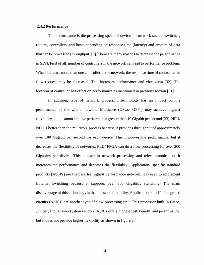
but it does not provide higher flexibility as shown in figure 2.4.

15

Figure 2.4 Network processing [3]

Therefore, hybrid approach is the perfect solution for the previous problems in

order to offer high flexibility and performance at the same time. For example, building

design that contains PLD, NPU/NFP, and CPU/GPP can produce hybrid programmable

platform [3]. Lookup performance has an impact on the performance. Packet switching

throughput can be improved up to 25% if commodity network interface cards are used in

Linux [34]. Improving hardware acceleration can lead to increase performance by 20%

[35]. Current implementation of OpenFlow switch leads to unacceptable performance, and

modification on OpenFlow protocol can increase the performance and reduce the overhead

[36], [37].

2.4.3 Security

Cyber-attacks have become a dangerous weapon against famous companies, banks,

government units, and universities. Malicious attack destroy, steal, expose, change, and

gain important information. Unfortunately, the SDN has problems and vulnerabilities that

16

attract attackers to perform their malicious actions. In general, there are many threat vectors

that are determined in SDN. These threat vectors in SDN and problems in the OpenFlow

model will be presented in the next two sections.

2.4.3.1 Threat Vectors in SDN

According to [8], there are seven types of threats vectors that are identified in the

SDN as shown in the figure 2.5. Some of these threats are specific to the SDN while others

are popular in the traditional networks as shown in table 1. The first threat vector fakes or

forges traffic flows that transfer between switches. Defective machine or malicious devices

may be the main cause for that threat. Attackers can use this vector to launch Denial of

Services attacks (DoS) against networking devices such as switches. The second threat

vector attacks switch devices. The main cause of this attack is vulnerability in switches

devices. By exploiting this threat, attackers can send traffic flows to other switches to

wreak havoc in the network. They can also slow down packets movement in the network.

Figure 2.5 Main threat vectors of SDN architectures [8]

17

The third threat vector attacks on the control plane communications. By exploiting

this threat, attackers can forge traffic flows and send many requests to the controller to

overload it. This generates the DDoS attacks toward controller. The main reason for this

attack is the weakness in TLS/SSL protocol [38]. The fourth vector attacks against the

control plane by exploiting the vulnerabilities in the controller. Attackers may bring down

the whole network if they can successful attack the control plane. The fifth threat is lack in

ability to establish a communication between management plane and controller. The third,

fourth, and fifth threat vectors are the most dangerous attacks because attackers can lunch

the DDoS attacks and bring down the whole system. These vectors are more specify to the

SDN as shown in table 1 [2], [8].

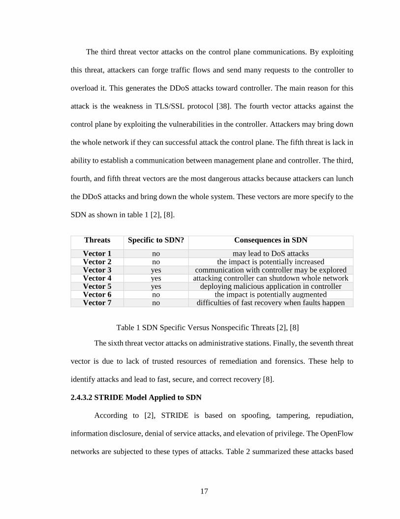
Threats Specific to SDN? Consequences in SDN

Vector 1 no may lead to DoS attacks Vector 2 no the impact is potentially increased Vector 3 yes communication with controller may be explored Vector 4 yes attacking controller can shutdown whole network Vector 5 yes deploying malicious application in controller Vector 6 no the impact is potentially augmented Vector 7 no difficulties of fast recovery when faults happen

Table 1 SDN Specific Versus Nonspecific Threats [2], [8]

The sixth threat vector attacks on administrative stations. Finally, the seventh threat

vector is due to lack of trusted resources of remediation and forensics. These help to

identify attacks and lead to fast, secure, and correct recovery [8].

2.4.3.2 STRIDE Model Applied to SDN

According to [2], STRIDE is based on spoofing, tampering, repudiation,

information disclosure, denial of service attacks, and elevation of privilege. The OpenFlow

networks are subjected to these types of attacks. Table 2 summarized these attacks based

18

on security properties and examples. First of all, spoofing is a malicious practice in which

attackers can hide their identity and send fake packets or traffic flows based on victim

identity to receiver. The main reason for this attack is lack of appropriate verification and

authentication [39]. Address Resolution Protocol (ARP) spoofing, ARP routing poisoning,

or ARP cashing poisoning is an example of spoofing technique. In the traditional networks,

attackers send their MAC address along with the IP address of victim to the switch in the

local network area (LAN). As a result, any traffic that have IP address of victim will be

directed to the machine of attackers. In this way, attackers may change traffic, intercept

data frame in the network, and stop flows traffic if they want. This process happens due to

lack of authentication to determine the verification of sender. This triggers many other

attacks such as man-in-the-middle (MITM), DoS, and session hijacking attacks [40]. In

SDN, the controller plays a role of forwarding packets functionality assuming that it has

information of MAC-IP mapping. The controller receives pairs of MAC address and IP

address of victim and forward them to targeted hosts or switches to store them in cash table

[41]. Finally, attackers can spoof controller address. This helps attackers to control the

whole network and install rules in the forwarding devices [2].

Attack Security

Property

Examples

Spoofing Authentication Forged ARP, IP and Mac address spoofing, and

IPv6 router advertisement.

Tampering Integrity Rule installation, counter falsification, and

modification affecting networking devices.

Repudiation Non-repudiation Modification for source address forgery and rule

installation.

Information

disclosure

Confidentiality Side channel attacks to explore flow rule setup.

DoS Availability Flow requests to overload control plane.

Elevation of

privilege

Authorization Control plane take over exploiting

implementation flaws.

19

Table 2: STRIDE attacks in OpenFlow networks [2]

In addition, tempering is another form of attack that target the OpenFlow network.

Attackers can intercept stored or transported data, and they can modify, change, remove

that information to serve their need. This attack compromises integrity because intruders

can do their actions without receiving alarms in all receivers. In SDN, intruders can

intercept and change OpenFlow controller communication, and they can overwrite the

controller rules [39]. Counter falsification is an example of this type of attack. Intruders try

to guess existed flow policy and then tamper packets to increase counter. This malicious

action increases billing for customer and takes nonoptimal decision by load balancing

algorithm [2].

Furthermore, repudiation is another type of attack in the SDN. Separating the

control plane from the data plane increases the probability to trace malicious nodes and

hidden communications [42]. However, attackers try to do malicious manipulation or

tempering that lead to change identification or authoring data in order to access the user to

wrong data. This is happened due to lack of monitoring capabilities and tracing of the

controller or networking devices in the SDN [39], [43].

Moreover, the OpenFlow network also faces an attack that is called information

disclosure. The goal of this attack is to collect information about system that is publicly

available such as path levels, response time, and version number. The main problem for

this attack is due to the lack of confidentiality that is responsible for preventing access to

certain information that open the door to expose sensitive information [39]. For example,

attackers can get information about network operation when rule flows setup is in place.

The controllers in the SDN install flow rules in switch in two different ways which are

either reactive or proactive. when the flow rules installation is reactive, this means that

20

installation is based on notifications or reports from switches. Attackers can measure the

delay between first flow and the next one. This creates an attack called fingerprinting which

is the first step to create DoS attack [44]. However, when the flow rules installation is

proactive, attackers cannot easily guess the forwarding flow rules, but it is still possible

[25].

Finally, the SDN presents problem of elevation of privilege attacks. Attackers can

have legitimate privilege of administrators. By using this attack, attackers can do what

administrators do such as opening and changing files and/or even changing user account.

Finally, there are no perfect deployment or application to decide whether a certain design

is strong or not. For example, while large scale data centers have been installed by Google

[45], they ignored the issue of conflicting application using internal conflict resolution and

single application blocks [46], [39].

2.5 DDoS Attacks and Countermeasures

The SDN also faces the DoS and/or DDoS attacks. The DoS attacks happen when

compromised host targets single system by sending flood of unnecessary traffics. The main

goal of this attack is to decrease system availability and prevent legitimate users from

accessing available services. If attackers use many hosts instead of only one to target single

system which is the controller, this is called DDoS attacks. DDoS has harmful

consequences on the controller of the SDN. For example, businessmen who are offering

online services can loss large amount of money if attackers can carry out DDoS

successfully against these services [47].

In the normal case of the SDN, when users tried to communicate with each other

within network, they first send packets to their switch that is connected to them. These

21

incoming new packets will search to find a match with information that are stored in switch

forwarding table. The reason for that is that each packet can know its destination. If there

are any match, packets follow rules that are associated with the match. For example,

dropping packets is one option if there is a match. Another option is forwarding packet to

its destination node. However, if there are no matching between packets and information

in switch forwarding table, then switch will forward these packets to controller in a form

of packet-in messages for processing and getting new flow rule. The communication

between switches and controller may be done by using OpenFlow protocol [24]. Controller

would decide whether to drop or forward packet to its destination. It is responsible for

handling new packets and sending new rules to switches [19].

Figure 2.6 DDoS attacks in SDN [12]

Considering the previous normal case in the SDN, attackers can lunch DDoS

attacks against the controller by following one of next two scenarios. First, attacker hosts

(let say A1 and A2) who are under one switch (let say sw1 that is explained in figure 2.6)

22

may send large number of new low-rate packets to their switch. IP addresses for these new

packets may also be spoofed and may not existed in switch flow table rules. As a result,

switch may generate many packet-in toward controller to get response. This makes the link

between compromised switch and the controller (CSL1 in figure 2.6) under congestion and

overload the controller with many new packet-in requests.

The second scenario is that attackers under multiple switches for same controller

(let say A1 to A5) send many new spoofed IP packets to their switches. This makes links

between these switches and controller (CSL1, CSL2, and CSL3) are all congested. This

creates an attack that is called blind DDoS attacks as stated in [48] . It is very hard to detect

because attack load is divided among switches. Finally, both cases result in denying

legitimate requests and decrease system availability [12].

Finally, DDoS attacks against the controller have several characteristics that make

identification process very hard to be done by conventional detection methods. First of all,

there is not many benefits of performing detection process in the switches because switches

may not be able to detect this attack completely. The reason for that is attackers may be

distributed and located under different switches, so switches receive low traffics which

seem to be normal. In addition, the controllers are not able to decide whether they are

affected by the DDoS attacks or not according to number of receiving traffics only because

attacks could be achieved by benign traffics. Furthermore, traditional detection methods of

DDoS attacks such as ICMP flooding, TCP SYN flooding, and HTTP flooding require to

have specific characteristics. However, traffics features that are generated toward the

controller in the SDN network are different from these knowing flooding. This makes it

impossible for traditional techniques to detect the DDoS attacks against the controller in

23

the SDN [6]. Therefore, this thesis focuses on finding a good detection method of DDoS

attacks.

DDoS is a difficult problem that needs a real solution due to the reasons that are

mentioned earlier. According to [12], the DDoS solutions can be classified to whether they

are intrinsic solutions which are focused on the SDN components and their functionality

elements or extrinsic solutions which are focused on network flows and their features.

These two main classifications can be also categorized to further classification. Intrinsic

solutions can be classified into scheduling-based and architectural-based. However,

extrinsic solutions can be categorized into statistical and machine learning based.

2.5.1 Intrinsic Solutions

According to [12], intrinsic solutions are these solutions that are focused on the

SDN components and their functionality elements. They can be divided to either

scheduling-based solutions or architectural-based solutions.

Scheduling-based solutions are one of the implementation to protect the controller

of the SDN. In [49], H, Shih-Wen et al proposed a solution based on using hash-based

mechanism that operates in the control plane to increase the scalability. Switches may

generate many packet-in messages toward the controller due to receiving malicious traffics

or legitimate traffics from hosts. This increases the congestion and makes the controller as

a bottleneck point. Scheduling-based solutions aim mainly to decrease the controller

overhead and increase the scalability and reliability. They also help to reduce the

transmission delay and failure in response in case of the congestion. These solutions are

based on using round-robin model that assigns incoming packets from switches to multiple

queues in the controller. The main disadvantage of these solutions is that they cannot

24

recognize the flash crowd, which is based on sending large number of legitimate flows,

from the DDoS attacks. This means they does not have a detection model for the DDoS

attacks [12].

Another solution based on scheduling was proposed in [50]. This solution was

based on providing different queues for each switch in controller to receive incoming

packets. This distributes the allocation of controller processing capacity among switches.

This helps to separate packets that are coming from infected switch and these from

uninfected switch. This makes the controller to work even if it is under DDoS attacks. This

was the main goal of this method because controller failures may stop the whole networks.

Although this method separates malicious flows from normal flows, it was not able to

distinguish DDoS attacks from flash crowd [12].

Architectural-based solutions are another way to protect the controller in the SDN

from DDoS attacks. First of all, C. Dharmendra et al in [51] proposed a solution to fix

security and load balancing in SDN. They proposed a model for decoupling application

monitoring and packet monitoring from each other. This method has two parts which are

main and secondary controller as shown in figure 2.7.

Figure 2.7 Proposed Controller Architecture in [51]

25

The advantage of this division is that secondary controller can take control if there

are failures in the main controller. On other hands, authors did not explain the detection

phase. Their design did not differentiate malicious from legitimate flows and consider

DDoS attacks and flash crowd identically [12].

Wang proposed FloodGuard which is a defensive method against DDoS attacks.

FloodGuard has two modules to do its job. The first one called proactive flow rules analyzer

which is in the control plane. In this stage, flow rules were derived in runtime based on

dynamic application tracking and symbolic execution. The main reason for this module

was to keep SDN running under DDoS attacks. The second module named packet

migration which is responsible to cash flows in switches then sending them to the controller

by using round- robin scheduling and rate limit. The main reason for this module was to

prevent congestion and process flows during flood without dropping out legitimate flows

[52].

Finally, control messages and monitoring traffics that are going back and forth

between controller and switches may increase congestion. As a result, Z. Adel et al in [53]

proposed a solution which is an orchestrator-based architecture for enhancing network-

security. This model separated controlling functionality from monitoring and put each one

in a module, and both of modules were controlled by an orchestrator. Some kinds of attacks

could be determined by getting access to some packets such as DDoS attacks, and this was

called low resolution attacks. However, other attacks could be resolved by getting access

to all packets in network such as ARP attack, and this was called high resolution attack.

Orchestrator entity decide which module should be enabled according to attack type to do

26

detection with the help of orchestrator instructions. On other hands, this method did not

totally mitigate the attack, and packets attack can still be used in the system [12].

2.5.2 Extrinsic Solutions

Extrinsic solutions are these solutions that are focused on network flows and their

features. They can be divided to either statistical or machine learning based solutions [12].

2.5.2.1 Statistical Based Solutions

First of all, statistical-based solutions are another approach to protect the controller

of the SDN. In [10], D. Kotani proposed a method which is packet-in filtering mechanism

to detect the DDoS attacks against the controller. This method was based on recoding the

values of packet header by switches before sending packet-in values to the controller.

Switches then filter out packets that are less important than others or have the same values

of recorded one. However, this method was inactive if the values of new packets header

that were generated by attackers are different from the recorded one [6].

In [54], P. Andres et al proposed a method that was called FlowFence to protect

control plane based on statistical solutions. In their approach, switches monitor their

interfaces to determine whether there is congestion or not by measuring which interface

consuming large bandwidth. Then, switches notify the controller if they identify a

congestion for a specific link. Because the controller is responsible for assigning bandwidth

for links between controller and its switches, the controller limits flow transmission rate

for the congested interface to prevent starvation. They believed that their method is simple,

efficient, fast, and prevented congestion. However, their method cannot prevent attacks

completely, and it only limited the flow transmission rate [12].

27

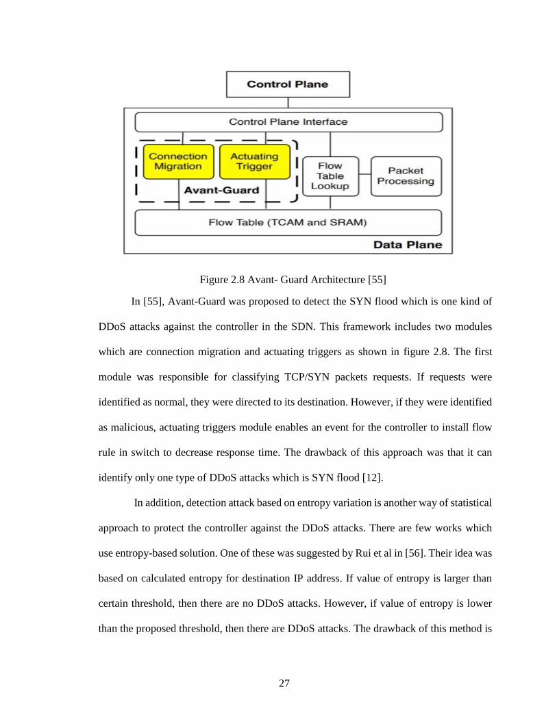
Figure 2.8 Avant- Guard Architecture [55]

In [55], Avant-Guard was proposed to detect the SYN flood which is one kind of

DDoS attacks against the controller in the SDN. This framework includes two modules

which are connection migration and actuating triggers as shown in figure 2.8. The first

module was responsible for classifying TCP/SYN packets requests. If requests were

identified as normal, they were directed to its destination. However, if they were identified

as malicious, actuating triggers module enables an event for the controller to install flow

rule in switch to decrease response time. The drawback of this approach was that it can

identify only one type of DDoS attacks which is SYN flood [12].

In addition, detection attack based on entropy variation is another way of statistical

approach to protect the controller against the DDoS attacks. There are few works which

use entropy-based solution. One of these was suggested by Rui et al in [56]. Their idea was

based on calculated entropy for destination IP address. If value of entropy is larger than

certain threshold, then there are no DDoS attacks. However, if value of entropy is lower

than the proposed threshold, then there are DDoS attacks. The drawback of this method is

28

that it could not separate malicious from legitimate packets [12]. However, this method

helped to achieve disturbed anomaly detection in the SDN and decrease congestion against

the controller [56].

Moreover, Chen in [9] proposed another way which is SDNShield to protect the

SDN against DDoS attacks. This defense framework was specified for protecting the SDN

network edges and the controller. First of all, SDNShield builds attack mitigation units

(AMU) which are array of software switches at the SDN network edges. These units help

to prevent the congestion or bottleneck at the SDN network edges. In addition, AMU helps

to protect the controller by installing two filtering platforms. The first one is statistical

differentiation (SD) which is responsible for separating the benign flows from malicious

flows. The second filter is TCP connection verification which is responsible in doing in-

depth investigation for false positive of the first step. This helps to make sure that benign

flows were accepted.

Furthermore, another solution for DDoS attacks which was based on anomaly

prevention techniques named a multi-criteria-based DDoS-attack prevention was

introduced in [57]. In this method, switches send statistical parameters to the controller

such as quantity of packets for each flow, numbers of flows entries, and arrival time. The

controller in turn receives these parameters and detects the DDoS attacks by using fuzzy

inference system and hard decision thresholds. This method could not only detect attacks

flows but also drop them based on demands from the control plane.

Finally, a new idea was suggested in [58] which was combining of OpenFlow and

sFlow module to detect and mitigate a DDoS attacks on the SDN. Authors of this paper

exploited the OpenFlow and sFlow protocol features to detect malicious flows in real time.

29

Their framework composed three components which were collector, anomaly detection,

and anomaly mitigation as shown in figure 2.9. First, they discovered that OpenFlow

approach increased communication between switches and the controller. This decreased

Figure 2.9 Architecture of DDoS Detection and Mitigation that Proposed in [58]

scalability and increased probability of the DDoS attacks against the control plane. Thus,

they used sFlow approach instead of OpenFlow approach to separate controller from data

collection process and decrease the data collected. Second, they used entropy-based

detection for separating malicious and normal flows in both OpenFlow approach and sFlow

approach. Third, using anomaly mitigation to block undesired attacks. This module had

several advantages. For example, the scalability was improved because they did not need

to collect large numbers of flows as in OpenFlow approach. Performance was increased

because CPU and memory flow cache usage were minimized. Finally, there were an

effective reduction in the communication between the controller and switches that

decreases the possibility of overloading the controller.

2.5.2.2 Machine Learning Based Solutions

Machine-learning-based-solutions are another approach to identify DDoS attacks

against the controller in the SDN. In these kinds of solutions, the defense mechanism that

was trained by feeding free attack flows (training) into machine learning algorithm can

30

detect attack flows (testing) [12]. Kokila et al. suggested a method to detect DDoS attacks

against the controller by using support vector machine (SVM) classifier [59].

SVM is one type of large margin classifier and kind of machine learning. It is used

primarily to find the decision boundary or a model that separates points to two or more

groups. For example, let us assume that we have a dataset of training samples, and each

point of these samples is marked as belong to one or another group. SVM creates a model

to separate these current data by drawing a clear decision boundary or gap that is as wide

as possible. The data points that created this boundary are called the support vector points.

Then, this model categorizes new datasets on the same space according to which side of

the gap they fall [60].

There are several intuitions behind the SVM. First, the large margin classifier may

help decrease the errors in calculation. This improves the classification task because points

that are located near the decision boundary have uncertain classification decision. In other

words, the uncertainty in the classification decision may be decreased by making the

margin large enough. Second, as long as the margin is large enough, the model may have

little choices of where data fit. As a result, the memory capacity may be decreased, and this

increases the ability to correctly classify data [60]. For these reasons, authors in [59] used

SVM as a classifier to detect DDoS attacks. They found that their algorithm is better than

other machine learning algorithms. However, their algorithm could only detect attacks

without trying to mitigate these attacks [12].

31

CHAPTER 3: METHODOLOGIES

This chapter explains flow classifications in the first part. In the second part, it

depicts algorithms that are used to identify the compromised switch interfaces and detect

DDoS attacks against the controller in the SDN. Sequential probability ratio test (SPRT),

count-based detection (CD), percentage-based detection (PD), entropy-based detection

(ED), and cumulative sum (CUSUM) are these algorithms.

3.1 Flow Classification

Flows are sequence of packets that share same characteristics. These characteristics

could be (source IP address, destination IP address, source port number, destination port

number, and/or protocol type). All of these information can be extracted from header of

each packet. Flows of TCP and UDP based protocols might be these five tuples. However,

flows of ICMP protocol could be grouping all packets that have same source IP address,

destination IP address, and protocol type because ICMP packets do not have port numbers

in their header.

Figure 3.1 Flow Sample from Wireshark about Flow [17]

For example, (172.16.116.194: 6222 -> 209.185.250.103: 80 TCP) is a TCP flow

sample from dataset that is called “outside tcpdump data” that was captured on the 5th day

of April in 1999 [17]. This flow has (9) packets which is simply explained steps of connect-

32

ion between two nodes. All of these packets share common information such as protocol

name, IP source address, IP destination address, destination port number, and source port

number. The first three packets are [SYN], [SYN/ACK], and [ACK] which are the three-

way handshaking in TCP to start connection. The fourth and fifth packets are exchanging

information. The last four packets are responsible to close the connection.

In SDN architecture, each switch has flow table that contains multiple flows entry.

Each entry has rule so that switch can know how to handle each incoming packet. When

users tried to communicate with others, they send packets to its switch. These incoming

packets are grouped to form flows. The incoming flows look at flow table in switch to find

a match. If there are a match between incoming flow and flow entry, incoming flow will

follow rule associated with flow entry. However, if there are no match, then a switch may

generate packet-in message toward the controller to get new flow rule. Finally, the

controller installs new flow rule in flow table so that switch can handle a flow [24], [19].

However, attackers could be located in any computer device as shown in figure 2.6.

They tend to send to their switch large number of new low-traffic flows that are not

presented in that switch flow table. The new flows will induce switch to generate many

packet-in messages toward the controller. This overloads the controller with large number

of requests and leads to the DDoS attacks. Attackers also tend to send low-traffic flows

because these flows will save attackers’ time to congest the controller [6].

The main aim of classification is to identify DDoS attacks by classifying these

flows to either low-traffic flows (malicious flows) or normal flows. Let consider (Foi ),

where (o) is a sequence observations of different flows (F) that injected an interface (i) of

the SDN switch. (Foi ) is low flow if total number of packets within this flow is lower than

33

or equal to certain threshold. However, (Foi ) is normal flow if total number of packets within

this flow is larger than that threshold. The (Foi ) can be defined as follow [6]:

(Foi )= {

1, if number of packets≤Threshold

0, if number of packets>Threshold (3.1)

3.2 Detection Algorithms

The main goal for this stage is to identify the affected interface. Five different type

of algorithms that were used to decide whether switch interface (i) is compromised or not.

3.2.1 Sequential Probability Ratio Test (SPRT)

SPRT is the first algorithm that was developed by Wald, and it is a

specific sequential hypothesis test based on mathematical calculation [61]. It uses two

hypothesizes which are H0 and H1. H0 means that interface is normal whereas H1 means

that interface of switch is compromised. The compromised interface (H1) is injected by

large number of low-traffic flows whereas normal interface is injected by large number of

normal flows.

In reality, detection process produces two types of error which are false positive

and false negative. False positive error is benign interfaces (H0) that are falsely identified

as compromised interfaces (H1). False negative error is the compromised interfaces (H1)

that are falsely identified as benign interfaces (H0). To avoid these two types of errors,

value of false positive error should not exceed a specified value of (α), and value of false

negative error should not exceed a specified value of (β).

In [6], SPRT was used to decide whether the interface (i) is compromised or not by

considering a sequence of (n) which is observation of normal and compromise flows (Foi )

where (o) is the series of observation (o=1,2,3,…,n). These sequences of flows observation

are obtained from the first stage which is flow classification. According to SPRT method,

https://en.wikipedia.org/wiki/Sequential_analysis

34

(Dni ) is a detection function that can be defined as a log-likelihood ratio of (n) flows

observation, whether they are normal flow or low-traffic flow, for certain interface (i).

Therefore, the equation for ( Dni ) is the following [6]:

Dni = ln

pr (F1i ,…., Fn

i |H1 )

pr ( F1i , …. , Fn

i |H0) (3.2)

Assuming (Foi ) is identically distributed and independent [6], Thus, Dn

i will be:

Dni =∑ ln

pr (Foi |H1 )

pr ( Foi |H0 )

n

o=1

(3.3)

Because Foi is a Bernoulli random variable [6],

pr ( Foi =1|H0 ) = 1- pr ( Fo

i =0|H0)=λ0 (3.4)

pr ( Foi =1|H1) =1-pr ( Fo

i =0|H1)=λ1 (3.5)

Where λ0 is less than λ1because normal interface is less likely to be injected with

low-traffic flows.

This detection can be a one-dimensional random walk. This means if Coi which is

total number of packets of Foi are less than or equal to certain threshold (which is 3) then

(Foi )=1 and the walk moves upward one step. However, if Co

i are larger than the threshold

then (Foi )=0 and the walk moves downward one step [6]. Therefore, the new equation for

Dni will be:

Dni =

{

Dn-1

i +lnpr (Fo

i =1|H1 )

pr ( Foi =1 |H0)

, Coi ≤threshold

Dn-1i +ln

pr (Foi =0|H1 )

pr ( Foi =0 |H0)

, Coi >threshold

35

=

{

Dn-1i +ln

λ1

λ0

, Coi ≤threshold

Dn-1i +ln

1-λ1

1-λ0

, Coi >threshold

(3.6)

Where D0i =1.

Now, the value of Dni compares each time with the upper threshold (A) and lower

threshold (B). If value of Dni is smaller or equal to (B), then the interface (i) is H0 and

terminate the test. If value of Dni is larger or equal to (A), then the interface (i) is H1 and

terminate test. Otherwise, monitor will continue with additional observation. The value of

(A) and (B) can be calculated as shown in equation (3.7) [6], [61]:

{

A=lnβ

(1-α)

B=ln(1-β)

α

(3.7)

3.2.2 Count-Based Detection (CD)

CD is another approach that is used to identify DDoS attacks and locate the

compromised interface. This method is based on the number of low-traffic flows. The result

of first step that is explained in (3.1) which is classifying flows to either low-traffic flows

or normal flows are used as an input to this method. In this method, normal flows are

ignored, and low-traffic flows are gathered into small groups or window size based on

either timeslot or number of packets. Number of low-traffic flows are calculated per group,

and the result is compared with certain threshold. If comparison result is larger or equal to

threshold, then attack is detected. However, there is no attack if result of comparison is

lower than threshold. Finally, comparison process will go through all groups to decide

whether certain interface is infected or not [6].

36

3.2.3 Percentage-Based Detection (PD)

PD is another method that is also used to detect DDoS attacks against the controller.

It also uses to determine whether interface is compromise or not. This method is based on

finding percentage of low-traffic flows. This method has two main components which are

windows size and threshold. First, the results of low-traffic flows classification from the

first stage are grouped to small groups size based on either number of packets or timeslots.

Second, percentages of low-traffic flows are calculated by dividing number of low-traffic

flows values over number of all flows (normal and low-traffic flows) per group. Third, the

results from each group is compared with certain threshold. If percentage of low-traffic

flows for one group is larger or equal to a suggested threshold, there is attack for this group.

However, if the result of comparison is lower than the threshold, then there is no attack.

The process will go through all small groups to find whether the interface is compromise

or not [6].

3.2.4 Entropy-Based Detection (ED)

Seyed and Marc proposed a detection method in [11] that is based on calculating

incoming packets’ entropy that is used to measure the randomness of these packets. When

incoming packets are random, the entropy may be high. However, when the randomness is

low, the entropy may be also low. This method has two main parts which are windows size

and threshold. Incoming packets need to be divided into small groups (windows) based on

either timeslot or number of incoming packets. Entropy is calculated for all elements in

each window. The value of entropy of each window compares with certain threshold to

measure randomness.

In this method, packets are classified to different flows according to certain

common of specification such as IP source address, IP destination address, port source

37

number, port destination number, and protocol type as mentioned earlier in flow

classification section. Then, destination IP address for the first packet of each unique flow

should be monitored. These monitored IP destination addresses are grouped in windows

(W). For each window, hash table of two column is created. The first column contains all

unique IP destination addresses, and second column contains number of times that each

unique IP appeared as shown in following equation:

W= {(x1, y1), (x2, y2), (x3, yi), ….} (3.8)

Let say (i) is denoting for each unique element in the window, and (n) is the total

number of all IP destination addresses for each window (W). Then, probability (P) of each

unique IP destination address is calculated as shown in following equation:

pi=

yi

n (3.9)

Entropy (E) for each window can be calculated in equation (3.10). Then, the value

of entropy may compare with certain threshold. if value of entropy is larger than the

threshold, this means there are no attacks. However, if value of entropy is smaller than the

threshold, this means there are attacks.

E= -∑ pi

ln pi

n

i=1

(3.10)

3.2.5 Cumulative Sum Detection (CUSUM)

CUSUM is an approach that is used to identify whether there is a small shift in the

process mean from certain target or not. It is a sequential analysis method that is introduced

by Page in [62]. CUSUM is the sum of accumulative samples that are deviated from target

(M0). If the results of summation are under certain threshold that is called decision interval

(H), this means the operation of process is normal and within the target. However, if the

38

result of accumulative sum is equal or larger than decision interval (H), this means the

process is out-of-control.

After flows are classified to either low-traffic flows or normal flow in the first step,

percentages of low-traffic flows (Xi) are calculated by dividing number of low-traffic flows

over number of all flows (normal and low-traffic flows) per timeslot. Target mean (M0) is

calculated by averaging all percentage values (dividing a summation of all percentage of

low-traffic flows values by their number). The accumulative deviation, which is the

summation of changes, can be calculated in two side. Upper side CUSUM ( Ci+) is

calculated when there are change in the upper or positive side whereas lower side CUSUM

(Ci-) is calculated when there are change in lower or negative side. The upper and lower

side CUSUM are computed as follow [62], [63]:

(Ci+) = Max [ 0, (Ci-1

+ ) +Xi- M0-K] (3.11)

(Ci-) = Min [ 0, (Ci-1

- ) +Xi- M0+K] (3.12)

Where C0+ and C0

- equal 0.

Allowance value or reference value which is (K) is chosen to be in middle of two

values. These two values are target mean (M0) and attack value of the mean (M1) that would

be detected fast. It can be computed as follow:

K= δ

2σ=

|M1-M0|

2 (3.13)

Where (σ) is the standard deviation that calculated based on target mean (M0)

whereas (δ) is computed as follow:

δ= |M1-M0|

σ (3.14)

39

If the value of upper side CUSUM (Ci+) and lower side CUSUM (Ci

-) is larger than

certain threshold (H), this means attack is detected. The value of (H) that suggested in [62]

and [64] computed as follow:

H= d k (3.15)

Where (d) is a function of false positive error (α), which is benign activities that are

falsely identify as attack or shift in process, and false negative error (β), which is amount

of shift or attacks that are falsely identified as benign. It is computed as follow:

d= 2

δ2 ln (

1-β

α) (3.16)

CUSUM method uses two counters which are (N+) and (N-) for (Ci+) and (Ci

-)

respectively to record when these two values start to increase above target mean (M0). (N+)

and (N-) increases by one when value of (Ci+) and (Ci

-) shifts away from target mean. The

reason for that is to know when attacks start to occur exactly by counting backward from

the time that (Ci+) and (Ci

-) values has exceeded (H) to time that these values start to shift

from (M0).

40

CHAPTER 4: RESULTS, EVALUATION AND DISCUSSION

4.1 Overview

This chapter presents the results of flow classification and detection algorithms that

are explained in the previous section. Java is the programming language that is used to

implement these algorithms. Defense Advanced Research Projects Agency (DARPA)

datasets are used to evaluate our works.

4.2 Datasets

The datasets that are available in the Lincoln Laboratory website [17] is used to

evaluate the detection algorithms. These datasets were captured by the group of Defense

Advanced Research Projects Agency (DARPA) to evaluate computer network instruction

detection systems. Some of these datasets were captured during 1998 while others were

captured during 1999. The datasets that were captured during 1998 have one router that

has one interface which is “00:00:0C:04:41:BC”. However, the datasets that were captured

during 1999 have one router that has one interface which is “00:10:7B:38:46:32”. All main

communications were passing through this interface. These two interfaces are considered

as SDN switch interface in our case. These interfaces generated packet-in messages toward

controller to overload it if they receive new flows from other interfaces that are connected

to them. Therefore, we filtered out communication among other interfaces because they do

not generate packet-in messages.

Four of these datasets were picked to do our evaluation, and they have the same

name which is (outside tcpdump data). To recognize among them, we depended on dates

41

of capturing these datasets. Therefore, datasets that were used in our evaluation are

(04/05/1999), (03/11/1999), (03/12/1999), and (07/03/1998).

4.3. Using Flows Classification in DARPA Dataset

We used jNetpcap library that is implemented in java to read packets from a dataset.

Packets were grouped to unique flows based on packet header information. Three multimap

tables of two columns and multiple rows were created to serve our needs. For the first

multimap table, first column stored all unique flows whereas second column stored all

packets that are belonged to each unique flow. As we mentioned earlier,

“00:00:0C:04:41:BC” is the only MAC address number for the SDN switch for datasets

that were captured during 1998. However, “00:10:7B:38:46:32” is the only MAC address

number for the SDN switch for datasets that were captured during 1999. From the first

multimap table, we need to get only flows that are injected to “00:00:0C:04:41:BC” if

dataset is chosen from 1998 and “00:10:7B:38:46:32” if dataset is chosen from 1999.

To do that, we checked whether first packet for each flow has this MAC address as

a destination address in their header or not. If this condition is yes, we created another

multimap table, and we saved these flows in first column and number of each unique flows

in the second column. However, we ignored the rest that do not have this condition. We

did that because we need to know who start the connection. If the destination address in

first packet is this MAC, we knew that switch interface is the receiver. Thus, if the receiver

receives low-traffic flows, then switch will generate packet-in toward controller.

Finally, we classified all flows that exist in the second map table to either normal

or low-traffic flows. We did that by comparing number of packets with certain threshold.

The threshold is chosen to be (3) because normal TCP flow has at least three packets which

42

are three-ways handshaking of TCP protocol [6]. Therefore, if number of packets that

belong to certain flow is larger than or equal to (3), the flow is normal, otherwise it is low-

traffic flow. For example, the flow shown in figure 3.1 is normal flow because total number

of packets are more than (3) packets. This process was applied to all flows that exist in the

second multimap table. The results of classification were stored in the third multimap table.

4.4 Flow Classification Results

In this section, we picked four datasets to evaluate and present result of flow

classification. These datasets are (04/05/1999), (03/11/1999), (03/12/1999), and

(07/03/1998).

4.4.1 Results of Flows Classification for (04/05/1999) Dataset

This dataset contains (1299771) packets that have different protocols in their

header. There are many types of DDoS attacks that were detected at different times in this

dataset as mentioned in [6]. After gathering these packets to different flows, we got (51376)

flows. Only (25762) have 00:10:7B:38:46:32 as destination in their first packet as shown

in figure (4.1). After classifying these flows, we got (20732) low-traffic flows and the rest

of them were normal as shown in table 3.

Table 3: Statistics of Classification Flows Phase for 1999 Datasets

Dataset

name

Number of

all packets

in each

dataset

Number

of all

Flows

Number of all flows that have

00:10:7B:38:46:32 as

destination in the first packet of

each flow

Number of low flows that have

00:10:7B:38:46:32 as


each flow

Number of normal flows that

have 00:10:7B:38:46:32 as


each flow

04/05/1999 1299771 51376 25762 20732 5030

03/11/1999 1339058 56725 14840 11482 3358

03/12/1999 1176620 49050 18055 15248 2807

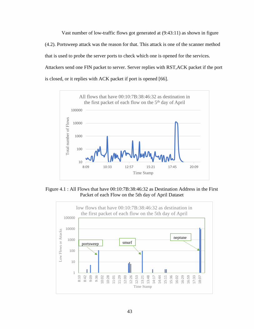
43

Vast number of low-traffic flows got generated at (9:43:11) as shown in figure

(4.2). Portsweep attack was the reason for that. This attack is one of the scanner method

that is used to probe the server ports to check which one is opened for the services.

Attackers send one FIN packet to server. Server replies with RST,ACK packet if the port

is closed, or it replies with ACK packet if port is opened [66].

Figure 4.1 : All Flows that have 00:10:7B:38:46:32 as Destination Address in the First

Packet of each Flow on the 5th day of April Dataset

10

100

1000

10000

100000

8:09 10:33 12:57 15:21 17:45 20:09

To

tal

num

ber

of

Flo

ws

Time Stamp

All flows that have 00:10:7B:38:46:32 as destination in

the first packet of each flow on the 5th day of April

1

10

100

1000

10000

100000

8:1

0

8:4

2

9:0

9

9:3

6

10

:02

10

:28

11

:01

11

:29

12

:00

12

:26

12

:53

13

:21

13

:48

14

:17

14

:44

15

:11

15

:36

16

:02

16

:29

16

:59

17

:33

18

:07

Lo

w F

low

s o

r A

ttac

ks

Time Stamp

low flows that have 00:10:7B:38:46:32 as destination in

the first packet of each flow on the 5th day of April

portsweep smurf

neptune

44

Figure 4.2: Low-Traffic Flows that have 00:10:7B:38:46:32 as Destination Address in

the First Packet of each Flow on the 5th day of April Dataset

Even though intrusion detection methods do not consider portsweep as DDoS

attacks, but attackers can use it to generate many low-traffic flows to trigger SDN switch

to generate packet-in messages to overload the controller as stated in [6]. These types of

scanners can pass through packet routers filtering and some type of firewalls [67] and lead

to actual dangers in the future [68]. Thus, it is very important to consider them as an attack.

In addition, smurf attack that occurred at (13:18:12) also generated many low-

traffic flows as shown in figure (4.2). Smurf uses spoofed IP that is usually like victim

machine. Attackers may direct victim machine to send an ICMP protocol that contains echo

asking for a reply to its broadcast address of its network. When victim does that, these IP

addresses may reply with echo response that makes network unusable [69].

Finally, neptune attacks generated many low-traffic flows at (18:04:04) as shown

in figure (4.2). In neptune attack, attacker sends SYN packets from its IP address or spoofed

IP address to server to hide his identity. Then, server responses with a SYN/ACK packets

to client, while client will not send back ACK packet. In this case, server may wait some

time for each connection, and this consumes server resources and drops legitimate requests

[70].


This dataset contains (1339058) packets that different protocols in their headers.

(56725) are the number of all flows after dividing these packets to unique flows as shown

in table 3. The number of all flows that have (00:10:7B:38:46:32) as a destination Address

in the First Packet of each Flow is (14840) as shown in figure (4.3).

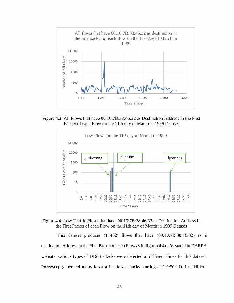
45

Figure 4.3: All Flows that have 00:10:7B:38:46:32 as Destination Address in the First

Packet of each Flow on the 11th day of March in 1999 Dataset


the First Packet of each Flow on the 11th day of March in 1999 Dataset

This dataset produces (11482) flows that have (00:10:7B:38:46:32) as a

destination Address in the First Packet of each Flow as in figure (4.4) . As stated in DARPA

website, various types of DDoS attacks were detected at different times for this dataset.

Portsweep generated many low-traffic flows attacks starting at (10:50:11). In addition,

10

100

1000

10000

100000

8:24 10:48 13:12 15:36 18:00 20:24

Num

ber

of

All

Flo

ws

Time Stamp

All flows that have 00:10:7B:38:46:32 as destination in

the first packet of each flow on the 11th day of March in

1999

1

10

100

1000

10000

100000

8:0

4

8:3

4

9:0

2

9:2

8

9:5

3

10

:22

10

:52

11

:19

11

:45

12

:12

12

:44

13

:14

13

:47

14

:13

14

:40

15

:11

15

:37

16

:02

16

:32

16

:59

17

:25

17

:54

18

:48

Lo

w F

Lo

ws

or

Att

acks

Time Stamp

Low Flows on the 11th day of March in 1999

portsweep neptune ipsweep

46

another attack which is neptune or SYN flood attack leaded also to produce vast low-traffic

flows at (11:04:16). Finally, at (16:36:10), ipsweep also generated many numbers of low

attacks. ipsweep is like a probe network technique. In the legitimate cases, admin of

network sends this probe to identify which machine is alive for the diagnosis purposes [68].

However, attackers can use this probe to serve its need. They can send to SDN switch large

amount of ICMP echo packets that lead to create a table miss. In turn, compromised switch

interface generates packet-in requests toward controller to overload it. This is kind of

DDoS attacks that overloads the controller and refuse legitimate requests.


This dataset has almost (1176620) packets. When we classified these packets to

different flows, we got almost (49050) flows as shown in table 3. Because only flows that

are injected to SDN switch would overload controller, we filtered out other flows. Thus,

we got (18055) as total number of flows that are injected to SDN switch as shown in figure

4.5. These total number in figure 4.5 can be classified into (15248) as low-traffic flows and

rest of them as normal. In figure 4.6, there are many new low-traffic flows that were

generated at (11:20:15) which is a neptune attack. Finally, portsweep is another attack that

produced low-traffic flows at 17:13:10.

47

Figure 4.5: All Flows that have 00:10:7B:38:46:32 as Destination Address in the First

Packet of each Flow on the 12th day of March in 1999 Dataset


the First Packet of each Flow on the 12th day of March in 1999 Dataset


This dataset has almost one million packets as shown in table 4. These packets can

be grouped to (256055) flows. The datasets that were captured during 1998 has one router

10

100

1000

10000

8:09 10:33 12:57 15:21 17:45 20:09

Num

ber

of

All

Flo

ws

Time Stamp

All Flows on the 12th day of March in 1999

1

10

100

1000

10000

8:0

7

8:3

8

9:0

7

9:3

3

10

:00

10

:30

11

:04

11

:32

12

:01

12

:27

12

:58

13

:30

14

:00

14

:26

14

:55

15

:21

15

:48

16

:16

16

:47

17

:15

17

:42

18

:11

Lo

w F

low

s

Time Stamp

low flows on the 12th of March in 1999

neptune portsweep

48

that has one interface which is “00:00:0C:04:41:BC”. Therefore, we need to get only these

flows that are injected to this interface, which is considered as SDN switch in our case. We

got (250551) flows that have this MAC address as destination in their first packet as shown

in figure (4.7).

Table 4: Statistics of Classification Flows phase for 1998 Dataset

Figure 4.7: All Flows that have 00:00:0C:04:41:BC as Destination Address in the First

Packet of each Flow for (07/03/1998) Dataset

There are many new low-traffic flows starting to occur at different time stamp for

this dataset as mentioned in DARPA website and shown in figure (4.8). First, portsweep

attack generated low flow starting at 11:46:39. Another attack which is neptune also

produced many new flows at 17:27:07. Finally, at 18:00:15, smurf attack has started to

occur as shown in figure below.

10

100

1000

10000

100000

8:09 10:33 12:57 15:21 17:45 20:09

All

Flo

ws

Time Stamp

All Flows for (07/03/1998)

Dataset

name

Number of all

packets in each

dataset

Number

of all

Flows

Number of all flows that have

00:00:0C:04:41:BC as

destination in the first packet

of each flow

Number of low flows that have

00:00:0C:04:41:BC as

destination in the first packet

of each flow

Number of normal flows that

have 00:10:7B:38:46:32 as


each flow

07/03/1998 1194920 256055 250551 243730 6821

49

Figure 4.8: Low-Traffic Flows that have 00:00:0C:04:41:BC as Destination Address in

the First Packet of each Flow for (07/03/1998) Dataset

4.5 Parameters of Detection Methods

First of all, SPRT needs four parameters in its algorithms as mentioned in section

(3.2.1). These parameters are β, α, λ0 and λ1. It is better to choose a small value of β and α

that are between 0.01 and 0.05 to limit the value of false negative error and false positive

error as mentioned in [6] and [65]. As a result, we set β to be equal to (0.02) and α to (0.01).

We also set λ0= 0.33 and λ1=0.6 because choosing these two values decreases the number

of low-traffic flows observations that are needed to decide whether interface is

compromised or not as mentioned in [6].

In addition, CD, PD, ED, and CUSUM depend on two important components which

are windows size and threshold. First, window size for CD, PD and CUSUM methods are

based on timeslot. We set their window size to be either almost every five minutes or ten

minutes. However, window size for ED method is based on packets number. As suggested

in [11] , number of packets in windows size should be set to be same as number of hosts in

1

10

100

1000

10000

100000

8:0

4

8:2

9

8:5

4

9:1

9

9:4

5

10

:10

10

:37

11

:03

11

:30

11

:57

12

:22

12

:49

13

:17

13

:43

14

:09

14

:35

15

:00

15

:26

15

:53

16

:18

16

:47

17

:17

17

:44

18

:09

18

:39

Lo

w F

low

s

Time Stamp

Low Flows for (07/03/1998)

portsweep

neptune

smurf

50

the network. Thus, we set that to be 10 packets because number of hosts in the network of

dataset is almost 10.

Second, we chose different threshold values which are 80, 150, and 250 in CD

method. However, threshold value of PD was set to the following values: 0.2, 0.5, and 0.8.

The reason for choosing different values is to observe reaction of each method with

different threshold. However, the threshold of ED should set to be either 1.31 or 0.2 as

suggested in [11] and [6]. Finally, M1 or threshold of CUSUM algorithm was set to be

either 0.4 or 0.8. We chose 0.4 because we need to detect out-of-control or low-traffic flows

average value quickly. We also assumed M1 to be 0.8 to compare results with previous

threshold.

4.6 Detection Methods Results and Discussion

This section presents and compares results of the detection algorithms. SPRT,

CD, PD, ED, and CUSUM are the detection algorithms that are used to show the results.

4.6.1 Results of Detection Algorithm for (04/05/1999) Dataset

On 5th of April 1999 dataset, three types of DDoS attacks named “portsweep”,

“smurf”, and “neptune” occurred at “9:43:11”, “13:18:12”, and “18:04:04” respectively.

All of these attacks produce vast and new of low-traffic flows as shown in figure (4.2).

Table.5 summarizes results of all detection methods for this dataset.

Detection Detected Attacks (√)

Name Window

size

Threshold Portsweep Smurf Neptune

SPRT - - √ √ √

CD 5-minutes 80 √ √ √

CD 5-minutes 150 √





51

PD 5-minutes 0.2 √ √ √

PD 5-minutes 0.5 √ √

PD 5-minutes 0.8 √

PD 10-minutes 0.2 √ √ √



ED 10 packets 0.2 √ √


CUSUM 5-minutes 0.4 √ √

CUSUM 5-minutes 0.8 √


CUSUM 10-minutes 0.8 √

Table 5: Detected Attacks for All Detection Methods for (04/05/1999) Dataset

First of all, SPRT was able to detect all of these attacks. SPRT could decide that

switch interface is compromised after observing only six continuous low-traffic flows. It

also took only ten continuous normal flows observation to decide that interface is normal.

These numbers are considered to be as minimum number of observations that are needed

to take a decision.

In addition, CD generated same results when we chose different timeslot and

produced different results when we chose different threshold. When we set threshold=80,

CD detected all attacks that were detected by SPRT method. However, CD detected only

“neptune” attack when threshold= 150 or 250. This means CD method produces false

negative when threshold is high. Thus, it is a challenge to choose certain threshold and

windows size to detect all attacks in CD method.

Furthermore, PD also depends on windows size and threshold in its

implementation. First, PD was not able to identify “smurf” attack and produce false

negative when we set windows size to 5-minute and choose threshold=0.5. When we

changed that threshold to 0.8 with the same windows size, PD produced false negative at

52

“9:43:11” and “13:18:12” respectively. However, when we modified threshold to 0.2 with

the same timeslot, PD method generated false positive at “12:15”. Second, when we set

timeslot to 10-minute with different threshold, we got different results. If threshold=0.2,

PD detected all attacks. When threshold was 0.5 or 0.8, PD detected only neptune attack.

Therefore, PD method has the same problem that is faced by CD method which is choosing

an appropriate threshold and window size to get good output.

Finally, ED method generated false positive at “10:29” and false negative at “9:43”

when windows size was 10 packets and threshold=1.31 or 0.2. CUSUM did not detect

portsweep attacks when M1 =0.8. It also identified “smurf” attack as a benign at “13:18”

whether M1=0.4 or 0.8. CUSUM faces difficulties of setting suitable windows size and

threshold value to get accurate results. Finally, we got different results from CD, PD, ED,

and CUSUM when we changed their main component values as shown results for 5th April

dataset. Thus, it is challenging to choose these values to get accurate results.


On 11th of March in 1999 dataset, three types of DDoS attacks named “portsweep”,

“neptune”, and “ipsweep” occurred at “10:50:11”, “11:04:16”, and “16:36:10”

respectively. All of these attacks generate new and vast number of low-traffic flows as

shown in figure (4.4). Table.6 summarizes results of all detection methods for this dataset.


Name Window

size

Threshold portsweep neptune ipsweep

SPRT - - √ √ √



CD 5-minutes 250 √ √


CD 10-minutes 150 √ √ √


53




PD 10-minutes 0.2 √ √ √

PD 10-minutes 0.5 √ √ √


ED 10 packets 0.2 √

ED 10 packets 1.31 √

CUSUM 5-minutes 0.4 √ √ √





First of all, SPRT identified all of these anomalies. The minimum number of low-

traffic flows observations that were helped SPRT to decide that switch interface is

compromise was only “6” whereas the maximum number of low-traffic flows observations

was “20”. However, the minimum number of normal flows observations to decide that

switch interface is normal was “10” whereas the maximum number was “19”.

Moreover, we used two timeslot sizes which are 5-minutes and 10-minutes with

different thresholds to evaluate CD and PD method as mentioned earlier. CD generated

false negative at “16:36:10” when timeslot and threshold were 5 or 10-minutes and 250

packets respectively. Furthermore, PD detected all attacks with window size of 5-minutes

and all proposed threshold. However, it generated false negative at “16:38” when we set

timeslot to10-minute and threshold=0.8.

Finally, ED was not able to detect “portsweep” and “neptune” and generated false

negative at “10:50:11” and “11:04:16” with both threshold 1.31 and 0.2. CUSUM method

identified all attacks on the 11th day of March dataset.

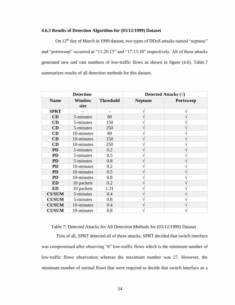
54


On 12th day of March in 1999 dataset, two types of DDoS attacks named “neptune”

and “portsweep” occurred at “11:20:15” and “17:13:10” respectively. All of these attacks

generated new and vast numbers of low-traffic flows as shown in figure (4.6). Table.7

summarizes results of all detection methods for this dataset.


Name Window

size

Threshold Neptune Portsweep

SPRT - - √ √




















First of all, SPRT detected all of these attacks. SPRT decided that switch interface

was compromised after observing “6” low-traffic flows which is the minimum number of

low-traffic flows observation whereas the maximum number was 27. However, the

minimum number of normal flows that were required to decide that switch interface as a

55

normal in this dataset was 10 whereas maximum number was 16. Finally, CD, PD, ED,

and CUSUM detected all attacks for this dataset as shown in table 7.


For this dataset, there are three attacks which are “portsweep”, “neptune”, and

“smurf” that were started to occur at “11:46:39”, “17:27:07”, and “18:00:15” respectively

as shown in figure (4.8). Table.8 summarizes results of all detection methods for this

dataset. First of all, SPRT detected “neptune” and “smurf” attack because they were

generated many new low-traffic flows. SPRT can decide that interface is compromised

after observing 6 continuous low-traffic flows which are considered to be as a minimum

number of observations whereas the maximum number of observation was 62. However,

the minimum number of normal flows that are required to decide that switch interface is

normal in this dataset is 10 whereas maximum number is 40.


Name Window

size

Threshold portsweep neptune smurf

SPRT - - √ √



















56


On other hands, SPRT method was not able to detect “portsweep” attack although

this attack produced low-traffic flows. This attack produces one low-traffic flow that was

coming from a port which is 1234 toward a port from a group of 1-100 port every three

minutes. This is like a DoS attack when an attacker attacks multiple machines from single

machine. There are many flows were generated every three minutes, and most of them were

normal flows. SPRT was taking its decision based on these normal flows. Thus, SPRT

produces false negative and fails to detect attacks when low-traffic flows are distributed

over long time periods. Finally, CD, PD, ED, and CUSUM failed to detect “portsweep”

and generated false negative at “11:46:39”.

4.7 Evaluation of Detection Method by Confusion Matrix

We used confusion matrix that is mentioned in [71] to evaluate and compare all

detection method. This matrix depends on four main components which are True Negative

(TN), False Positive (FP), False Negative (FN), and True positive (TP). From these

elements, many metrics can be computed. First of all, true positive rate (TPR) is the rate of

number of malicious activities that are truly classified by classifier method as malicious. It

also called sensitivity or recall, and it can be calculated from the following equation:

TPR=TP

TP+FN (4.1)

True negative rate (TNR) is the rate of number of benign activities that are truly

classified by classifier method as benign. It also called specificity, and it can be computed

from the following equation:

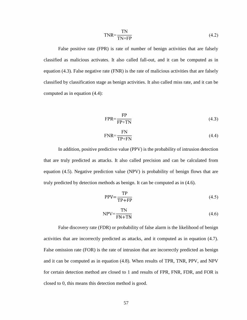
57

TNR=TN

TN+FP (4.2)

False positive rate (FPR) is rate of number of benign activities that are falsely

classified as malicious activates. It also called fall-out, and it can be computed as in

equation (4.3). False negative rate (FNR) is the rate of malicious activities that are falsely

classified by classification stage as benign activities. It also called miss rate, and it can be

computed as in equation (4.4):

FPR=FP

FP+TN (4.3)

FNR=FN

TP+FN (4.4)

In addition, positive predictive value (PPV) is the probability of intrusion detection

that are truly predicted as attacks. It also called precision and can be calculated from

equation (4.5). Negative prediction value (NPV) is probability of benign flows that are

truly predicted by detection methods as benign. It can be computed as in (4.6).

PPV=TP

TP+FP (4.5)

NPV=TN

FN+TN (4.6)

False discovery rate (FDR) or probability of false alarm is the likelihood of benign

activities that are incorrectly predicted as attacks, and it computed as in equation (4.7).

False omission rate (FOR) is the rate of intrusion that are incorrectly predicted as benign

and it can be computed as in equation (4.8). When results of TPR, TNR, PPV, and NPV

for certain detection method are closed to 1 and results of FPR, FNR, FDR, and FOR is

closed to 0, this means this detection method is good.

58

FDR=FP

TP+FP (4.7)

FOR=FN

FN+TN (4.8)

Finally, Accuracy of detection methods can be calculated as in equation (4.9).

Prevalence is another metric, and it measures number of attacks affecting particular

population of dataset. It can be computed as in (4.10). Because accuracy metric is not a

good method to assess the performance of classifier or detection test, F1 score can be used

as another metric to measure accuracy of detection. It is a harmonic average of recall and

precision, and it can be computed as in (4.11). It is between 0 and 1. When F1 score is 0,

performance of classifier is worst whereas when it is 1, performance of classifier is best.

Accuracy=TP+TN

TP+TN+FN+FP (4.9)

Prevalence=TP+FN

TP+TN+FN+FP (4.10)

F1 score= 2. PPV+TPR

PPV+TPR (4.11)

4.7.1 Confusion Matrix Results for (04/05/1999) Dataset

Confusion matrix for this dataset was computed for all detection method to compare

between them. First of all, we calculated TPR, FPR, TNR, FNR, PPV, FDR, FOR, and

NPV for all detection methods. These values are between 0 and 1. The values of TPR,

TNR, PPV, and NPV for SPRT method are very closed to 1 and results of FPR, FNR, FOR,

and FDR for this detection method is very closed to 0 as shown in figure 4.9. This means

this detection method is good. ED method has almost same results. However, value of FPR

59

is 0.35 and TNR is 0.64 for this method whether threshold was 1.31 or 0.2 as shown in

figure 4.9.a and figure 4.9.b respectively.

CD, PD, and CUSUM produced very low TPR and very high FNR as shown in

figure 4.9.a and figure 4.9.b respectively. CUSUM also produced 0.3 to 0.4 of FDR and

0.6 to 0.7 for PPV as shown in figure 4.9.c. Finally, we used abbreviation for all detection

methods as shown in table 9 to make figure 4.8, figure 4.9, and figure 4.10 more clear.

Abbreviation Name of Detection Window size Threshold

A SPRT - -

B CD 5-minutes 80

C CD 5-minutes 150

D CD 5-minutes 250

E CD 10-minutes 80

F CD 10-minutes 150

G CD 10-minutes 250

H PD 5-minutes 0.2

I PD 5-minutes 0.5

J PD 5-minutes 0.8

K PD 10-minutes 0.2

L PD 10-minutes 0.5

M PD 10-minutes 0.8

N ED 10 packets 0.2

O ED 10 packets 1.31

P CUSUM 5-minutes 0.4

Q CUSUM 5-minutes 0.8

R CUSUM 5-minutes 0.4

S CUSUM 5-minutes 0.8

Table 9: Abbreviation for All Detection Methods

60

Figure 4.9 Graph Showing (a) TPR vs. FPR, (b) TNR vs. FNR, (c) PPV vs. FDP, (d)

FOR vs. NPV for All Detection Methods for (04/05/1999) Dataset

Finally, values of prevalence, accuracy, and F1 score were presented in table 10.

The value of prevalence for both SPRT and ED were the same which is 0.80 whereas the

values of the rest were between 0.09 to 0.34. The value of accuracy and F1 score were 99%

for SPRT which means it is a good detection method. ED had 92% of accuracy and 95%

of F score. However, values of these two metrices for CD and PD were different. For

example, value of accuracy of CD and PD was between 0.69 and 0.84 whereas value of F

score was low. Finally, accuracy for CUSUM was between 70% to 80% whereas F score

was between 0.23 to 0.29.

A

B,P

C,D,J

E,K

F,G,L,M

H

I,Q

N,O

R,S

0

0.2

0.4

0.6

0.8

1

0 0.2 0.4 0.6 0.8 1

TPR

, Rec

all,

Sen

siti

vity

FPR, Fall-Out(a)

A

B,R,S C,D,J

E,F,G,L,M

H

IK

N,O

PQ

0

0.2

0.4

0.6

0.8

1

0 0.2 0.4 0.6 0.8 1

Tru

e N

egat

ive

Rat

e

False Negative Rate(b)

A

B,C,D,E,F,G,H,I,J,K,L,M,R,S

N,O

PQ

0

0.2

0.4

0.6

0.8

1

0 0.2 0.4 0.6 0.8 1

PP

V, P

reci

sio

n

FDR, Probability of False Alarm(c)

A

B,I,P

C,D,J,Q

E,K

F,G,L,M

HN,O

R,S

0

0.2

0.4

0.6

0.8

1

0 0.2 0.4 0.6 0.8 1

Neg

ativ

e P

red

icti

ve V

alu

e

False Omission Rate(d)

61

Detection

Prevalence

Accuracy

F1 score Name Window

size

Threshold

SPRT - - 0.80 0.99 0.99

CD 5-minutes 80 0.19 0.84 0.32

CD 5-minutes 150 0.19 0.82 0.17

CD 5-minutes 250 0.19 0.82 0.17

CD 10-minutes 80 0.34 0.72 0.34

CD 10-minutes 150 0.34 0.69 0.19

CD 10-minutes 250 0.34 0.69 0.19

PD 5-minutes 0.2 0.19 0.85 0.38

PD 5-minutes 0.5 0.19 0.83 0.25

PD 5-minutes 0.8 0.19 0.82 0.17

PD 10-minutes 0.2 0.34 0.72 0.34

PD 10-minutes 0.5 0.34 0.69 0.19

PD 10-minutes 0.8 0.34 0.69 0.19

ED 10 packets 0.2 0.80 0.92 0.95

ED 10 packets 1.31 0.80 0.92 0.95

CUSUM 5-minutes 0.4 0.19 0.82 0.29

CUSUM 5-minutes 0.8 0.19 0.81 0.23

CUSUM 10-minutes 0.4 0.34 0.7 0.27

CUSUM 10-minutes 0.8 0.34 0.7 0.27


(04/05/1999) Dataset


The values of TPR, FPR, TNR, FNR, PPV, FDR, FOR, and NPV were calculated

for all detection method for this dataset as shown in figure (4.10). First of all, SPRT

produced high values of TPR, TNR, PPV, and NPV whereas it generated low values of

FPR, FNR, FOR, and FDR. This is an indication that this detection method is good.

However, ED has same results of SPRT, except that it produced high value of FOR and

NPV as shown in figure 4.10.d.

62


(d) FOR vs. NPV for All Detection Methods for (03/11/1999) Dataset

Moreover, values of TPR for these PD, CD, CUSUM methods were almost between

0.2 to 0.4 as shown in figure 4.10.a whereas their values of FNR were between 0.53 to 0.8

as shown in figure 4.10.b. Finally, CUSUM generated low value of PPV and high value of

FDR when threshold = 0.4 and window size = 5-minutes as shown in figure 4.10.c.

Finally, SPRT had 99% of accuracy and F score whereas ED has 81% and 86% for

accuracy and of F score respectively as shown in table 11. On other hands, CD, PD, and

CUSUM had accuracy between 82% and 93%, but the values of F score are between 33%

and 63% which explains why these methods did not detect some DDoS attacks.

A

B,H,I

C,D

E,K,L

F,G,M

J

N,O

P

Q

RS

0

0.2

0.4

0.6

0.8

1

0 0.2 0.4 0.6 0.8 1

TPR

, Rec

all,

Sen

siti

vity

FPR, Fall-Out (a)

AB,H,I

C,DE,K,L

F,G,MJ

N,O

P

Q

R

S

0

0.2

0.4

0.6

0.8

1

0 0.2 0.4 0.6 0.8 1

Tru

e N

egat

ive

Rat

e


A

B,C,D,E,F,G,H,I,J,K,L,M

N,O

S

R

P

Q

0

0.2

0.4

0.6

0.8

1

0 0.2 0.4 0.6 0.8 1

PP

V, P

reci

sio

n

FDR, Probability of False Alarm(b)

A

B,H,I,P,Q

C,DE,K,L

F,G,M

J

N,O

R,S

0

0.2

0.4

0.6

0.8

1

0 0.2 0.4 0.6 0.8 1

Neg

ativ

e P

red

icti

ve V

alu

e


63

Detection

Prevalence

Accuracy

F1 score Name Window

size

Threshold

SPRT - - 0.77 0.99 0.99

CD 5-minutes 80 0.11 0.93 0.63

CD 5-minutes 150 0.11 0.91 0.37

CD 5-minutes 250 0.11 0.91 0.37

CD 10-minutes 80 0.17 0.89 0.57

CD 10-minutes 150 0.17 0.85 0.33

CD 10-minutes 250 0.17 0.85 0.33

PD 5-minutes 0.2 0.11 0.93 0.63

PD 5-minutes 0.5 0.11 0.93 0.63

PD 5-minutes 0.8 0.11 0.92 0.47

PD 10-minutes 0.2 0.17 0.89 0.57

PD 10-minutes 0.5 0.17 0.89 0.57

PD 10-minutes 0.8 0.17 0.85 0.33

ED 10 packets 0.2 0.77 0.81 0.86

ED 10 packets 1.31 0.77 0.81 0.86

CUSUM 5-minutes 0.4 0.11 0.83 0.38

CUSUM 5-minutes 0.8 0.11 0.83 0.38

CUSUM 10-minutes 0.4 0.17 0.82 0.37

CUSUM 10-minutes 0.8 0.17 0.85 0.42


(03/11/1999) Dataset


SPRT generated high levels of specificity, sensitivity, precision, and NPV that are

near to 1. It also produced low levels of fall out, miss rate, probability of false alarm, and

FOR that are near to 0. This seems to be best case scenario that a good detection method

should produce as shown on figure 4.11. ED had almost same results, except that values of

specificity, NPV, and FOR is 0.88, 0.85, and 0.1 respectively as shown in figure 4.11.a and

figure 4.11.d.

64



In addition, CD, PD, and CUSUM produced very bad sensitivity which is almost 0

instead of 1 as shown in figure 4.11.a. They also had value of miss rate close to 1 instead

of 0 as shown 4.11.b. CUSUM produced values between 02 to 0.4 of FOR. Finally, it

generated low level of PPV and high level of FDP as in 4.11.c.

Finally, table 12 shows results of prevalence, accuracy, and F1 score. First of all,

SPRT and ED produced good value of these metrices. In addition, PD, CD, and CUSUM

A

B,C,D,H,I,J

E,F,G,K,L,M

N,O

P,SQ,S

0

0.2

0.4

0.6

0.8

1

0 0.2 0.4 0.6 0.8 1

TPR

, Rec

all,

Sen

siti

vity

FPR, Fall-Out (a)

A

B,C,D,E,F,G,H,I,J,K,L,M

N,O

P

Q,RS

0

0.2

0.4

0.6

0.8

1

0 0.2 0.4 0.6 0.8 1

PP

V, P

reci

sio

n


A

B,C,D,H,I,J

E,F,G,K,L,M

N,OP

Q

R

S

0

0.2

0.4

0.6

0.8

1

0 0.2 0.4 0.6 0.8 1

Tru

e N

egat

ive

Rat

e


A

B,C,D,H,I,J,P,Q

E,F,G,K,L,M

N,O

R

S

0

0.2

0.4

0.6

0.8

1

0 0.2 0.4 0.6 0.8 1

Neg

ativ

e P

red

icti

ve V

alu

e


65

had values of prevalence between 0.24 and 0.43. They also had bad results of F1 score

which are between 0.29 and 0.32, and their accuracies between 56% to 80%.

Detection

Prevalence

Accuracy

F1 score Name Window size Threshold

SPRT - - 0.84 0.99 0.99

CD 5-minutes 80 0.24 0.80 0.32

CD 5-minutes 150 0.24 0.80 0.32

CD 5-minutes 250 0.24 0.80 0.32

CD 10-minutes 80 0.43 0.64 0.29

CD 10-minutes 150 0.43 0.64 0.29

CD 10-minutes 250 0.43 0.64 0.29

PD 5-minutes 0.2 0.24 0.80 0.32

PD 5-minutes 0.5 0.24 0.80 0.32

PD 5-minutes 0.8 0.24 0.80 0.32

PD 10-minutes 0.2 0.43 0.64 0.29

PD 10-minutes 0.5 0.43 0.64 0.29

PD 10-minutes 0.8 0.43 0.64 0.29

ED 10 packets 0.2 0.84 0.95 0.97

ED 10 packets 1.31 0.84 0.95 0.97

CUSUM 5-minutes 0.4 0.24 0.73 0.33

CUSUM 5-minutes 0.8 0.24 0.75 0.27

CUSUM 10-minutes 0.4 0.43 0.56 0.20

CUSUM 10-minutes 0.8 0.43 0.60 0.27


(03/12/1999) Dataset


This dataset likes other previous datasets in which SPRT and ED had good results

of TPR, FPR, TNR, FNR, PPV, FDP, NPV, and FOR as shown in figure 4.12. The only

exception is that ED had 0.72 of NPV and 0.27 of FOR, but it is still better than other

detections methods.

66



PD, CD, and CUSUM had low values of TPR and high value if FNR as shown in

figure 4.12.a and figure 4.12.b respectively. Finally, SPRT and ED had 99% of accuracy

and F1 score. PD, CD, and CUSUM had accuracies between 45% to 53% and F1 score

between 23% to 31%.

A

B,C,D,H,I,J

E,F,G,K,L,M

N,O

P,Q

R,S0

0.2

0.4

0.6

0.8

1

0 0.2 0.4 0.6 0.8 1

TPR

, Rec

all,

Sen

siti

vity

FPR, Fall-Out (a)

A

B,C,D,H,I,J

E,F,G,K,L,M

N,O

PQ

R

S

0

0.2

0.4

0.6

0.8

1

0 0.2 0.4 0.6 0.8 1

Tru

e N

egat

ive

Rat

e


AB,C,D,E,F,G,H,I,J,K,L,M

N,O P,Q

RS

0

0.2

0.4

0.6

0.8

1

0 0.2 0.4 0.6 0.8 1

PP

V, P

reci

sio

n


A

B,C,D,H,I,J

E,F,G,K,L,M

N,O

P,Q

R,S

0

0.2

0.4

0.6

0.8

1

0 0.2 0.4 0.6 0.8 1

Neg

ativ

e P

red

icti

ve V

alu

e


67

Detection

Prevalence

Accuracy

F1 score Name Window size Threshold

SPRT - - 0.97 0.99 0.99

CD 5-minutes 80 0.56 0.53 0.29

CD 5-minutes 150 0.56 0.53 0.29

CD 5-minutes 250 0.56 0.53 0.29

CD 10-minutes 80 0.60 0.50 0.31

CD 10-minutes 150 0.60 0.50 0.31

CD 10-minutes 250 0.60 0.50 0.31

PD 5-minutes 0.2 0.56 0.53 0.29

PD 5-minutes 0.5 0.56 0.53 0.29

PD 5-minutes 0.8 0.56 0.53 0.29

PD 10-minutes 0.2 0.60 0.50 0.31

PD 10-minutes 0.5 0.60 0.50 0.31

PD 10-minutes 0.8 0.60 0.50 0.31

ED 10 packets 0.2 0.97 0.98 0.99

ED 10 packets 1.31 0.97 0.98 0.99

CUSUM 5-minutes 0.4 0.56 0.49 0.26

CUSUM 5-minutes 0.8 0.56 0.49 0.26

CUSUM 10-minutes 0.4 0.6 0.45 0.23

CUSUM 10-minutes 0.8 0.6 0.47 0.27


(07/03/1998) Dataset

68

CHAPTER 5: CONCLUSION

5.1 Conclusion

The SDN makes networks design more flexible, cheaper, and programmable

because it separates the control plane from the data plane. The SDN gives administrators

of networks more flexibility to handle the whole network by using one device which is the

controller. Unfortunately, the controller of the SDN faces the dangers of DDoS attacks.

Attackers trigger their switches to generate large number of packet-in messages toward

controller when they send new and vast numbers of low-traffic flows to switches. This

leads to DDoS attacks against the SDN controller. DDoS attacks can reduce system

availability and bring the network down.

We conducted a comparative study of a set of methods for detecting the DDoS

attacks on the controller of SDN and identifying compromised switch interfaces. Because

attackers generated new and low-traffic flows, flows were classified to either low-traffic

flows or normal flows. Results of classification were as an input for detection methods.

These methods are SPRT, CD, PD, ED, and CUSUM. These methods are based on

statistical approaches. DARPA dataset were used to evaluate these methods. The datasets

that were used in our evaluation are (04/05/1999), (03/11/1999), (03/12/1999), and

(07/03/1998).

In addition, CD, PD, ED, and CUSUM have two main components: windows size

and threshold. These algorithms need to divide dataset to small window sizes that are based

69

on either timeslot or packets number. The window size of CD, PD, and CUSUM was based

on timeslot whereas window size for ED was based on number of packets. Table 14 shows

the overall mean of detected attacks for all detection methods. First of all, the overall mean

of detected attacks for SPRT was 0.91. Furthermore, the overall mean of detected attacks

for CD and PD fall between 0.66 and 0.91 whereas overall average of detected attacks for

CUSUM fall between 0.74 and 0.83. Finally, ED has 0.66 of overall average of detected

attacks.

Detection

Overall

Mean Name Window

size

Threshold

SPRT - - 0.91

CD 5-minutes 80 0.91






PD 5-minutes 0.2 0.91






ED 10 packets 0.2 0.66

ED 10 packets 1.31 0.66

CUSUM 5-minutes 0.4 0.83




Table 14: Overall Mean of Detected Attacks for all Datasets

We found that SPRT had 99% of accuracy and F score which means it is good

detection method. Values of TPR, TNR, PPV, and NPV for all datasets were almost closed

to 1 whereas values of FPR, FNR, FOR, and FDR were almost closed 0. SPRT detected

70

all attacks without producing false positive or false negative when sequence of continuous

low-traffic flows was generated for certain amount of time. However, SPRT produced

false negative and failed to detect attacks when low-traffic flows were distributed over

long time periods as shown on the 3th day of July in 1998 dataset.

ED produced different results for each dataset. It had accuracy values that fall

between 81% and 98% whereas F score values fall between 86% and 99%. This method

generated values of FOR that fall between 0 and 0.44 whereas values of FPR fall between

0 and 0.35. Values of FNR and FDR close to 0. However, values of TPR and PPV close

to 1. Finally, values of TNR fall between 1 and 0.64 whereas NPV values fall between 1

and 0.55. ED was not able to detect some DDoS attacks such as portsweep on the 5th day

of April in 1999 dataset, portsweep and neptune on the 11th day of March in 1999 dataset,

and portsweep for 3th day of July in 1998 dataset.

In addition, CD and PD methods produced low number of TPR and high number

of FNR. This decreases both of accuracy and F score values. The values of accuracy for

CD and PD fall between 50 and 93 whereas values of F score fall 29 and 63. Moreover,

CUSUM method has values of accuracy fall between 45 and 83 whereas values of F score

fall between 20 and 42. Finally, PD, CD, and CUSUM algorithms produced different

results when values of their components were changed. They are also failed to detect some

attacks. Therefore, it is challenging to set appropriate values of window size or threshold

to get accurate detection results.

5.2 Future Work

For future work, I am planning to study other new methods based on statistical

approaches to discover their effectiveness to detect the DDoS attacks and protect the

71

controller of the SDN. I am also planning to explore the machine learning algorithms to

determine their ability in identifying the DDoS attacks against the controller of the SDN.

72

REFERENCES

[1] B. Raghavan et al., "Software-defined internet architecture: Decoupling architecture

from infrastructure," Proc. 11th ACM Workshop Hot Topics Netw., p. 43–48, 2012.

[2] D. Kreutz et al., "Software-Defined Networking: A Comprehensive Survey,"

Proceedings of the IEEE, vol. 103, no. 1, pp. 14-76, 2015.

[3] S. Sakir et al., "Are we ready for SDN? Implementation challenges for software-

defined networks," IEEE Communications Magazine, pp. 36-43, 2013.

[4] H. Kim and N. Feamster, "Improving network management with software defined

networking," IEEE Communications Magazine, vol. 51, no. 2, pp. 114-119, 2013.

[5] N. Zhang, H. Hämmäinen and H. Flinck, "Cost efficiency of SDN-enabled service

function chaining," info, vol. 18, no. 5, pp. 45-55, 2016.

[6] D. Ping et al. , "A detection method for a novel DDoS attack against SDN controllers

by vast new low-traffic flows," IEEE International Conference on Communications

(ICC), 2016.

[7] "SDN architecture issue 1," Open Networking Foundation, pp. 1-68, 2014.

[8] D. Kreutz, F. Ramos and P. Veríssimo, "Towards Secure and Dependable Software

Defined Networks," Proceedings of the second ACM SIGCOMM workshop on Hot

topics in software defined networking. ACM, pp. 55-60, 2013.

[9] C. Kuan-yin et al, "SDNShield: Towards More Comprehensive Defense against DDoS

Attacks on SDN Control Plane," 2016 IEEE Conference on Communications and

Network Security (CNS), pp. 28-36, 2016.

73

[10] D. Kotani and Y. Okabe, "A Packet-In Message Filtering Mechanism for Protection

of Control Plane in OpenFlow Networks," 2014 ACM/IEEE Symposium on

Architectures for Networking and Communications Systems (ANCS) Architectures for

Networking and Communications Systems (ANCS), 2014 ACM/IEEE Symposium on,

pp. 29-40, 2014.

[11] S. M. Mousavi and M. St-Hilaire, "Early Detection of DDoS Attacks against SDN

Controllers," International Conference on Computing, Networking and

Communications, Communications and Information Security Symposium, pp. 77-81,

2015.

[12] K. Kalkan, G. Gür and F. Alagöz , "Defense Mechanisms against DDoS Attacks in

SDN Environment," IEEE Communications Magazine, vol. 55, no. 9, pp. 175-179,

2017.

[13] S. Shin et al, "Rosemary: A Robust, Secure, and High-Performance Network

Operating System," ACM SIGSAC Conference on Computer and Communications

Security (CCS'14), Scottsdale, AZ., pp. 78-89, 2014.

[14] A. Durresi and M. Karakus, "A survey: Control plane scalability issues and approaches

in Software-Defined Networking (SDN)," Computer Networks, vol. 112, pp. 279-293,

2017.

[15] K. Nagase, "Software Defined Network Application in Hospital," InImpact: The

Journal of Innovation Impact, vol. 6, pp. 1-11, 2013.

[16] S. Sorensen, "Security implications of software-defined networks," Fierce Telecom,

14 May 2012. [Online]. Available: http://www.fiercetelecom.com/telecom/security

implications-software-defined-networks.

74

[17] "MIT Lincoln Laboratory," Intrusion detection atttacks database, [Online]. Available:

https://ll.mit.edu/ideval/index.html.

[18] T. Benson, A. Akella and D. Maltz, "Unraveling the complexity of network

management," Proc. 6th USENIX Symp. Networked Syst. Design Implement., p. 335–

348, 2009.

[19] M. Nick et al., "OpenFlow: Enabling innovation in campus networks," Acm Sigcomm

Computer Communication, vol. 38, no. 2, pp. 69-74, 2008.

[20] N. Feamster, Rexford, J and Zegura, E, "The Road to SDN: An Intellectual History of

Programmable Networks," ACM SIGCOMM COMPUTER COMMUNICATION,

vol. 44, no. 2, pp. 87-98, 2013.

[21] N. Handigol et al., "Reproducible network experiments using container based

emulation," Proceedings of the 8th International Conference Emerging Networking

Experiments & Technologies, pp. 253-264, 2012.

[22] B. Lantz, B. Heller and N. McKeown, "A Network in a Laptop: Rapid Prototyping for

Software-Defined Networks," Proceeding Hotnets-IX Proceedings of the 9th ACM

SIGCOMM Workshop on Hot Topics in Networks, pp. 1-6, 2010.

[23] "SDN Architecture Overview Version 1.0," Open Networking Foundation, pp. 1-5,

2013.

[24] "OpenFlow Switch Specification Version 1.1.0 Implemented," Open Networking

Foundation, pp. 1-56, 2011.

[25] R. Kloti, V. Kotronis and P. Smith, "OpenFlow: A Security Analysis," Network

Protocols (ICNP), 2013 21st IEEE International Conference, 2013.

[26] M. Hill, "What is Scalabiliy?," ACM SIGARCH Computer Architecture News, vol.

75

18, no. 4, pp. 18-21, 1990.

[27] A. Bondi, "Characteristics of scalability and their impact on performance,"

Proceedings of the 2nd international workshop on Software and performance, pp. 195-

203, 2000.

[28] A. Shalimov et al., "Advanced study of SDN/OpenFlow controllers," ACM

International Conference Proceeding Series, pp. 1-6, 2013.

[29] T. Benson, A. Akella and D. Maltz, "Network traffic characteristics of data centers in

the wild," Proceedings of the 10th Annual Conference: Internet Measurement, pp. 267-

280, 2010.

[30] S. Kandula et al, "The nature of data center traffic: Measurements & analysis,"

Proceedings of the 9th ACM SIGCOMM Conference on Internet Measurement

Conference, pp. 202-208, 2009.

[31] B. Heller, N. McKeown and R. Sherwood, "The controller placement problem," ACM

SIGCOMM COMPUTER COMMUNICATION REVIEW, pp. 473-478, 2012.

[32] Y. Gourhant and V. D. Philip, "Cross-control: A scalable multi-topology fault

restoration mechanism using logically centralized controllers," IEEE 15th International

Conference High Performance Switching and Routing (HPSR), pp. 57-63, 2014.

[33] R. Ozdag, "Intel Ethernet Switch FM6000 Series - Software Defined Networking,"

Intel Corporation, pp. 1-8.

[34] M. Jarschel et al, "Modeling and Performance Evaluation of an OpenFlow

Architecture," Proceedings of the 2011 23rd International Teletraffic Congress, pp. 1-

7, 2011.

[35] Y. Luo et al., "Accelerating OpenFlow switching with network processors," Proceedi-

76

ngs of the 5th ACM/IEEE Symposium on Architectures for Networking and

Communications Systems, pp. 70-71, 2009.

[36] C. Andrew et al, "DevoFlow: Scaling Flow Management for High-Performance

Networks," SIGCOMM '11 Proceedings of the ACM SIGCOMM, vol. 41, no. 4, pp.

254-265, 2011.

[37] A. Bianco, R. Birke, L. Giraudo and M. Palacin, "OpenFlow Switching: Data Plane

Performance," 2010 IEEE International Conference on Communications

Communications (ICC), pp. 23-27, 2010.

[38] R. Holz et al, "X.509 Forensics: Detecting and Localising the SSL/TLS Men-in-the

Middle," Computer Security - ESORICS, pp. 217-234, 2012.

[39] F. Ruffy, W. Hommel and F. . v. Eye, "A STRIDE-based Security Architecture for

Software-Defined Networking," ICN 2016: The Fifteenth International Conference on

Networks, pp. 95-101, 2016.

[40] V. Ramachandran and S. Nandi, "Detecting ARP Spoofing: An Active Technique,"

ICISS'05 Proceedings of the First international conference on Information, pp. 239-250

, 2005.

[41] A. Talal et al, "Securing ARP in Software Defined Networks," IEEE 41st Conference

on Local Computer Networks, pp. 523-526, 2016.

[42] A. Bates et al, "Let SDN be your eyes: Secure forensics in data center networks," in

Proceedings of the 2014 NDSS Workshop on Security of Emerging Network

Technologies, ser. SENT14, pp. 1-7, 2014.

[43] K. Benton et al, "OpenFlow Vulnerability Assessment," in Proceedings of the Second

ACM SIGCOMM Workshop on Hot Topics in Software Defined Networking, ser. H-

77

otSDN’13, pp. 151-152, 2013.

[44] S. Shin and G. Gu, "Attacking Software-Defined Networks: A First Feasibility Study,"

Proceeding HotSDN '13 Proceedings of the second ACM SIGCOMM workshop on

Hot topics in software defined networking, pp. 165-166, 2013.

[45] S. Jain et al, "B4: Experience with a Globally-deployed Software Defined Wan," in

Proceedings of the ACM SIGCOMM 2013 Conference on SIGCOMM, ser.

SIGCOMM’13, pp. 3-14, 2013.

[46] P. Porras et al, "Securing the Software-Defined Network Control Layer," in

Proceedings of the 2015 Network and Distributed System Security Symposium, ser.

NDSS’15, 2015.

[47] A. Doyal, J. Zhan and H. A. Yu, "Towards Defeating DDoS Attacks," 2012

International Conference on Cyber Security cybersecurity Cyber Security, pp. 209-212,

2012.

[48] D. Ma, Z. Xu and D. Lin, "Defending Blind DDoS Attack on SDN Based on Moving

Target Defense," International Conference on Security & Privacy in Communication

Networks, pp. 463-480, 2015.

[49] H, Shih-Wen et al, "Design a Hash-Based Control Mechanism in vSwitch for

Software-Defined Networking Environment," IEEE International Conference on

Cluster Computing, pp. 498-499, 2015.

[50] S. Lim et al., "Controller scheduling for continued SDN operation under DDoS

attacks," Engineering, Electrical & Electronic, vol. 51, no. 16, p. 1259–1261, 2015.

[51] D. Chourishi, A. Miri, M. Milic´ and S. Ismaeel, "Role-Based Multiple Controllers

for Load Balancing and Security in SDN," IEEE Canada International Humanitarian

78

Technology Conference (IHTC) , 2015.

[52] H. Wang, L. Xu and G. Gu, "FloodGuard: A DoS Attack Prevention Extension in

Software-Defined Networks.," 2015 45th Annual IEEE/IFIP International Conference

on Dependable Systems & Networks, pp. 239-250, 2015.

[53] Z. Adel et al, "OrchSec: An Orchestrator-Based Architecture For Enhancing Network-

Security Using Network Monitoring And SDN Control Functions," Network

Operations and Management Symposium (NOMS), 2014 IEEE, pp. 1-9, 2014.

[54] P. Andres et al , "FlowFence: A Denial of Service Defense System for Software

Defined Networking," Proc. Global Info. Infrastructure Networking Symp, pp. 1-6,

2015.

[55] S. Seungwon et al, "Avant -Guard: Scalable and Vigilant Switch Flow Management

in Software-Defined Networks," Proc. 2013 ACM SIGSAC Conf. Computer &

Commun. Security, ACM , p. 413–424, 2013.

[56] R. Wang, Z. Jia and L. Ju, "An Entropy-Based Distributed DDoS Detection

Mechanism in Software-Defined Networking," 2015 IEEE

Trustcom/BigDataSE/ISPA, pp. 310-317, 2015.

[57] T. Phan et al, "A Multi-Criteria-based DDoS-Attack Prevention Solution using

Software Defined Networking," 2015 International Conference on Advanced

Technologies for Communications (ATC), pp. 308-313, 2015.

[58] K. Giotis et al, "Combining OpenFlow and sFlow for an effective and scalable

anomaly detection and mitigation mechanism on SDN environments," Computer

Networks 62, pp. 122-136, 2014.

[59] R. Kokila et al, "“DDoS Detection and Analysis in SDNBased Based Environment

79

Using Support Vector Machine Classifier," Proc. 2014 IEEE Sixth Int’l. Conf.

Advanced Computing, pp. 205-210, 2014.

[60] C. D. Manning, P. Raghavan and H. Schütze, Introduction to Information Retrieval,

England: Cambridge University Press, 2009.

[61] A. Wald, Sequential Analysis, New York: John Wiley and Sons, Inc., 1947.

[62] P. E. S, "Continuous Inspection Schemes," Biometrika Office, University College,

London, pp. 100-115, 1954.

[63] Montgomery, Douglas, C., Introduction to Statistical Quality Control, United States

of America.: John Wiley & Sons, Inc., 2009.

[64] "NIST/SEMATECH e-Handbook of Statistical Methods," 1 6 2003. [Online].

Available: http://www.itl.nist.gov/div898/handbook/. [Accessed 16 10 2017].

[65] J. Postel, "STD 7 RFC 793," September 1981. [Online]. Available: https://www.rfc-

editor.org/rfc/rfc793.txt. [Accessed 21 October 2017].

[66] G. Lyon, "Nmap," 2001. [Online]. Available: https://nmap.org/book/man-port-

scanning-techniques.html. [Accessed 21 October 2017].

[67] L. Teo, "Network Probes Explained: Understanding Port Scans and Ping Sweeps,"

Linux Journal, pp. 1-2, 2000.

[68] "1998 CERT Advisories," 05 January 1998. [Online]. Available:

https://www.cert.org/historical/advisories/CA-1998-01.cfm?. [Accessed 21 October

2017].

[69] "Software Enginnering Institute," 19 September 1996. [Online]. Available:

https://www.cert.org/historical/advisories/CA-1996-21.cfm?. [Accessed 21 October

2017].

80

[70] R. Radharamanan et al, "Sensitivity analysis on the CUSUM method," International

Journal of Production Economics, Elsevier, vol. 33, no. 1-3, pp. 89-95, 1994.

[71] “Confussion Matrix,” 7 August 2017. [Online]. Available:

https://en.wikipedia.org/wiki/Confusion_matrix. [Accessed 11 November 2017].

detection of ddos attacks against the sdn controller using ... · of attacks. ddos attacks on the...

Documents