detection of defects in polyurethane fabrics based on ... · abstract school of engineering...
TRANSCRIPT
MASTER THESIS
Detection of defects in polyurethanefabrics based on computer vision
techniques.
Author:
Rafael Angel Villegas
Miranda
Director:
Dr. Hernan Darıo Benıtez
Restrepo.
Department of Electronics and Computer Science
February 2015

i

ii
iii

iv

Abstract
School of Engineering
Department of Electronics and Computer Science
Master of Engineering
Detection of defects in polyurethane fabrics based on computer vision
techniques.
by Rafael Angel Villegas Miranda
Quality inspection is one of the most important aspects of modern industrial manufac-
turing of textiles. Nonetheless, at some companies this inspection is manual, expensive,
and oversights defects in textiles. These issues have a negative impact on companies’
productivity. The purpose of this applied research project is to detect the most costly
defects that occur in fabrics made from polyurethane, by using computer vision and
analysis of digital images obtained in controlled environments. The objects of interest
in these images correspond to cloth cuttings used to manufacture car chairs. There are
two topics to be addressed in this work. These are the automatic classification of cloths
and detection of defects in fabrics. Genetic algorithms find the optimal parameters in
Gabor filter banks. Receiving operating curve (ROC) and area under curve (AUC) are
the figures of merit used for evaluate the performance of the proposed system with re-
spect to manually segmented images. Results show that the computer based systems
accomplishes true positive rates greater than 90% for the inspected fabric types.
Keywords: computer vision, automated vision system, textiles, digital image processing,
fabric defects, textile fabrics.

Acknowledgements
The author expresses their acknowledgments to:
Hernan Darıo Benıtez Restrepo, PhD in Engineering and thesis Director, for his dedi-
cation and excellent guidance.
Albeiro Aponte Vargas, for his time and permission to use the front base of the calibra-
tion process.
vi

Contents
Abstract v
Acknowledgements vi
Contents vii
List of Figures x
List of Tables xii
Abbreviations xiii
1 INTRODUCTION 1
1.1 Introduction . . . . . . . . . . . . . . . . . . . . . . . . . . . . . . . . . . . 1
1.2 Description of the Research Problem . . . . . . . . . . . . . . . . . . . . . 2
1.3 Justification . . . . . . . . . . . . . . . . . . . . . . . . . . . . . . . . . . . 2
1.4 General Objective . . . . . . . . . . . . . . . . . . . . . . . . . . . . . . . 3
1.5 Specific Objectives . . . . . . . . . . . . . . . . . . . . . . . . . . . . . . . 3
1.6 Project Scope . . . . . . . . . . . . . . . . . . . . . . . . . . . . . . . . . . 4
1.7 Expected Project Results . . . . . . . . . . . . . . . . . . . . . . . . . . . 4
2 THEORETICAL FRAMEWORK 5
2.1 Previous works and theoretical background. . . . . . . . . . . . . . . . . . 5
2.1.1 Statistical Approaches . . . . . . . . . . . . . . . . . . . . . . . . . 8
2.1.2 Spectral Approaches . . . . . . . . . . . . . . . . . . . . . . . . . . 8
2.1.3 Model-Based Approaches . . . . . . . . . . . . . . . . . . . . . . . 8
2.2 Camera Calibration . . . . . . . . . . . . . . . . . . . . . . . . . . . . . . 10
2.2.1 Image Formation . . . . . . . . . . . . . . . . . . . . . . . . . . . . 12
2.2.2 Homogeneous coordinates . . . . . . . . . . . . . . . . . . . . . . . 13
2.2.3 Perspective projection . . . . . . . . . . . . . . . . . . . . . . . . . 13
2.2.4 Homogeneous transformation . . . . . . . . . . . . . . . . . . . . . 16
2.2.5 Camera parameters . . . . . . . . . . . . . . . . . . . . . . . . . . 18
2.2.5.1 Intrinsic parameters . . . . . . . . . . . . . . . . . . . . . 18
2.2.5.2 Extrinsic parameters . . . . . . . . . . . . . . . . . . . . . 19
2.2.6 Lens distortions . . . . . . . . . . . . . . . . . . . . . . . . . . . . . 20
2.2.6.1 Radial distortion . . . . . . . . . . . . . . . . . . . . . . . 20
2.2.6.2 Tangential distortion . . . . . . . . . . . . . . . . . . . . 21
vii

Contents viii
2.3 Illumination systems . . . . . . . . . . . . . . . . . . . . . . . . . . . . . . 21
2.4 Fabrics and selection of defects . . . . . . . . . . . . . . . . . . . . . . . . 23
2.4.1 Main defects ranking . . . . . . . . . . . . . . . . . . . . . . . . . . 25
2.4.2 Defects criteria selection . . . . . . . . . . . . . . . . . . . . . . . . 25
3 DEFECT DETECTION AND FABRICS REPRESENTATION 29
3.1 Defect detection in fabrics . . . . . . . . . . . . . . . . . . . . . . . . . . . 29
3.1.1 Gabor filters . . . . . . . . . . . . . . . . . . . . . . . . . . . . . . 29
3.1.1.1 Gabor filter selection method . . . . . . . . . . . . . . . . 33
3.1.1.2 Defect detection . . . . . . . . . . . . . . . . . . . . . . . 34
3.1.1.3 Gabor filter parameters . . . . . . . . . . . . . . . . . . . 34
3.2 Feature extraction for fabrics representation . . . . . . . . . . . . . . . . . 35
3.2.1 Fabric recognition based on minimum distance classifiers . . . . . . 37
3.2.2 Preprocessing . . . . . . . . . . . . . . . . . . . . . . . . . . . . . . 38
3.2.3 Training and validation data sets . . . . . . . . . . . . . . . . . . . 39
3.2.4 Segmentation . . . . . . . . . . . . . . . . . . . . . . . . . . . . . . 42
3.2.5 Simple thresholding . . . . . . . . . . . . . . . . . . . . . . . . . . 43
4 RESULTS AND ANALYSIS 44
4.1 Description of the proposed system . . . . . . . . . . . . . . . . . . . . . . 44
4.2 Camera Calibration . . . . . . . . . . . . . . . . . . . . . . . . . . . . . . 44
4.2.1 Experimental set-up . . . . . . . . . . . . . . . . . . . . . . . . . . 44
4.2.2 Results - comparison manual method . . . . . . . . . . . . . . . . . 49
4.2.3 Experiments and results of calibration process. . . . . . . . . . . . 50
4.2.3.1 Parameters of the function CalibrateCamera (OpenCV) . 52
4.2.3.2 Re-projection error estimation . . . . . . . . . . . . . . . 53
4.2.4 Evaluation of inspection methods . . . . . . . . . . . . . . . . . . . 57
4.2.5 Evaluation procedure . . . . . . . . . . . . . . . . . . . . . . . . . 58
4.3 Parameter tuning for Gabor filter banks and simple thresholding approach 59
4.3.1 Gabor filters . . . . . . . . . . . . . . . . . . . . . . . . . . . . . . 60
4.3.2 Simple thresholding . . . . . . . . . . . . . . . . . . . . . . . . . . 65
4.4 Results . . . . . . . . . . . . . . . . . . . . . . . . . . . . . . . . . . . . . . 67
4.4.1 Analysis of results . . . . . . . . . . . . . . . . . . . . . . . . . . . 67
4.4.1.1 Gabor filters method . . . . . . . . . . . . . . . . . . . . 67
4.4.1.2 Simple thresholding . . . . . . . . . . . . . . . . . . . . . 68
5 CONCLUSIONS AND FUTURE WORK 75
5.1 Conclusions . . . . . . . . . . . . . . . . . . . . . . . . . . . . . . . . . . . 75
5.2 Future Work . . . . . . . . . . . . . . . . . . . . . . . . . . . . . . . . . . 76
A Front system 77
B Prototype (C.E.) 80
C Developer Guide 82

Contents ix
D User guide 85
Bibliography 90

List of Figures
2.1 Point Grey - Flea3 FL3-GE-20S4C-C Camera. . . . . . . . . . . . . . . . . 11
2.2 Edmunds Optics - 6 mm Compact Fixed Focal Length Lens. . . . . . . . . 12
2.3 Pinhole model with identification of key variables . . . . . . . . . . . . . . 12
2.4 Modeling perspective projection [1] . . . . . . . . . . . . . . . . . . . . . . 14
2.5 Relationship between world and image coordinates. . . . . . . . . . . . . . 14
2.6 Final position (translation and rotation) . . . . . . . . . . . . . . . . . . . 16
2.7 Order of applying parameters from the real world to the camera . . . . . 20
2.8 Example of radial distortion (barrel distortion). [2] . . . . . . . . . . . . . 20
2.9 Tubular bulb, T8 led 22W - 1.20 m. . . . . . . . . . . . . . . . . . . . . . 23
2.10 Selected fabric images . . . . . . . . . . . . . . . . . . . . . . . . . . . . . 27
2.11 Selected images of defective fabrics. . . . . . . . . . . . . . . . . . . . . . . 28
3.1 Components of a Gabor function in spatial domain. . . . . . . . . . . . . 31
3.2 Gabor filter parameters . . . . . . . . . . . . . . . . . . . . . . . . . . . . 35
3.3 Features extraction from training set. . . . . . . . . . . . . . . . . . . . . 37
3.4 Features extraction process diagram with test set (Individual). . . . . . . 38
3.5 Mean graph - karyatide fabric (75 images). . . . . . . . . . . . . . . . . . 40
3.6 Variance graph - kariatyde fabric (75 images). . . . . . . . . . . . . . . . . 41
3.7 Kurtosis graph - kariatyde fabric (75 images). . . . . . . . . . . . . . . . . 41
3.8 Skewness graph - kariatyde fabric (75 images). . . . . . . . . . . . . . . . 42
3.9 Final graph representation for five fabrics types (75 images by fabric). . . 43
4.1 General process diagram. . . . . . . . . . . . . . . . . . . . . . . . . . . . 45
4.2 Geometric projections - pinhole model. . . . . . . . . . . . . . . . . . . . . 46
4.3 a) Area calculated by trigonometric projections - Pinhole model. b) Ef-fective area with an additional margin of 5% for lighting. . . . . . . . . . 48
4.4 Inspection areas. . . . . . . . . . . . . . . . . . . . . . . . . . . . . . . . . 48
4.5 Proposed prototype from a front view. . . . . . . . . . . . . . . . . . . . . 49
4.6 Markers on the table. . . . . . . . . . . . . . . . . . . . . . . . . . . . . . 49
4.7 Chessboard calibration pattern 5 x 4. . . . . . . . . . . . . . . . . . . . . . 51
4.8 Parameters for Calibration Process - (Flea3 FL3-GE-20S4C-C Color GigECamera). . . . . . . . . . . . . . . . . . . . . . . . . . . . . . . . . . . . . 52
4.9 Sample images for the calibration process . . . . . . . . . . . . . . . . . . 54
4.10 Identification of corners during the calibration process . . . . . . . . . . . 54
4.11 Values of the parameters obtained in the calibration process . . . . . . . . 55
4.12 Shapes selecting for testing. . . . . . . . . . . . . . . . . . . . . . . . . . . 55
4.13 Manual measurement of circle diameter D=120 mm. . . . . . . . . . . . . 56
4.14 ROC curve distribution. . . . . . . . . . . . . . . . . . . . . . . . . . . . . 57
x

List of Figures xi
4.15 Kariatyde fabric defect and manual segmentation . . . . . . . . . . . . . . 58
4.16 ROC curves (individuals) for petit point gray fabric. . . . . . . . . . . . . 59
4.17 AUC curve for images of fabric petit point red fabric (mean = 0.90876,standard deviation = 0.02488). . . . . . . . . . . . . . . . . . . . . . . . . 60
4.18 Simple thresholding result and manual segmentation. . . . . . . . . . . . . 60
4.19 Diagram process - Gabor filters method . . . . . . . . . . . . . . . . . . . 61
4.20 Diagram process - simple thresholding method . . . . . . . . . . . . . . . 62
4.21 a)angle=0.00, frequency=0.125, α=2.449, σx=3.567, σy=0.433; b) an-gle=0.0, frequency=0.306, α=2.449, σx=1.456, σy=0.439; c) angle=0.0,frequency=0.750, α=2.449, σx=0.594, σy=0.476 . . . . . . . . . . . . . . . 63
4.22 a)angle=1.0471, frequency=0.1250, α=2.449, σx=3.567, σy=0.433; b) an-gle=1.0471, frequency=0.306, α=2.449, σx=1.456, σy=0.439; c) angle=1.0471,frequency=0.750, α=2.449, σx=0.594, σy=0.476 . . . . . . . . . . . . . . . 63
4.23 a)angle=2.0943, frequency=0.1250, α=2.449, σx=3.567, σy=0.433; b) an-gle=2.0943, frequency=0.306, α=2.449, σx=1.456, σy=0.439; c) angle=2.0943,frequency=0.750, α=2.449, σx=0.594, σy=0.476 . . . . . . . . . . . . . . . 63
4.24 Diagram process - genetic algorithm. . . . . . . . . . . . . . . . . . . . . . 66
4.25 Inspection process results - Kariatyde fabric (training set). . . . . . . . . . 69
4.26 Inspection process results - Kariatyde fabric (test set). . . . . . . . . . . . 69
4.27 Inspection process results - Vulcron vinyl W/L fabric (training set). . . . 70
4.28 Inspection process results - Vulcron vinyl W/L fabric (test set). . . . . . . 70
4.29 Inspection process results - Vulcron vinyl N/L fabric (training set). . . . . 71
4.30 Inspection process results - Vulcron vinyl N/L fabric (test set). . . . . . . 71
4.31 Inspection process results - petit point gray fabric (training set). . . . . . 72
4.32 Inspection process results - petit point gray fabric (test set). . . . . . . . . 72
4.33 Inspection process results - petit point red fabric (training set). . . . . . . 73
4.34 Inspection process results - petit point red fabric (test set). . . . . . . . . 73
A.1 Calibrate Camera option. . . . . . . . . . . . . . . . . . . . . . . . . . . . 77
A.2 Defect inspection option. . . . . . . . . . . . . . . . . . . . . . . . . . . . . 78
A.3 Representation (Identification fabric type) option. . . . . . . . . . . . . . 79
C.1 Entity-relation model. . . . . . . . . . . . . . . . . . . . . . . . . . . . . . 83
C.2 Chessboard pattern - 9x7 squares. . . . . . . . . . . . . . . . . . . . . . . 84
D.1 Use case camera calibrate . . . . . . . . . . . . . . . . . . . . . . . . . . . 86
D.2 Use case fabric representation . . . . . . . . . . . . . . . . . . . . . . . . . 87
D.3 Use case Inspection (fabric defect detection process) . . . . . . . . . . . . 88
D.4 Use case Inspection (fabric defect detection process) . . . . . . . . . . . . 89

List of Tables
2.1 Fabric defect detection methods. . . . . . . . . . . . . . . . . . . . . . . . 10
2.2 Hardware . . . . . . . . . . . . . . . . . . . . . . . . . . . . . . . . . . . . 11
2.3 Camera specifications . . . . . . . . . . . . . . . . . . . . . . . . . . . . . 11
2.4 Preferred sustained luminance levels for different locations or visual tasks- Encyclopedia of health and safety at work [3]. . . . . . . . . . . . . . . . 22
2.5 Information provided by the manufacturer of T8 LED Tube 22W. . . . . . 23
2.6 Ranking of the main defects on fabrics occurred between January andSeptember 2013 detected by human inspection . . . . . . . . . . . . . . . 25
2.7 Main defects selected under the criterion of the highest cost . . . . . . . . 26
3.1 Statistical features for fabric representation . . . . . . . . . . . . . . . . . 40
3.2 Confusion matrix for test identification fabrics (rows are the true class) . 40
4.1 Values obtained by geometry - pinhole model (meters). . . . . . . . . . . . 49
4.2 Values obtained by direct measurement of the projection (meters) . . . . 50
4.3 Measurement of the distance between the camera and the object (square). 55
4.4 Measurement of circle diameter D=120 mm. . . . . . . . . . . . . . . . . . 56
4.5 Fabric images and inspection process details . . . . . . . . . . . . . . . . . 74
xii

Abbreviations
TP True Positive
FP False Positive
LF Lamination Failure
CF Carving Failure
OP Optimal Point
LG Lamination Growth
SP Stained Piece
mm millimeters
OS Operating System
AUC Area Under Curve
DB DataBase
CE Controlled Environment
GLCM Grey Level Co-occurrence Matrix
CCD Charge Coupled Device
xiii

Chapter 1
INTRODUCTION
1.1 Introduction
The variety of fabric defects, which can change within the same sample, makes it difficult
to automatically detect defects in textiles. The defective raw material that goes unde-
tected along the production represents a waste of time, labor force, storage, packaging,
and transportation. These drawbacks decrease company profit and generate misimpres-
sions on customer or end users. For example, some chairs manufacturing companies have
manual quality inspection systems, which overlook defects in textiles. These issues cause
a negative impact on productivity. Therefore, the goal of this applied research project is
to identify the most costly defects that may occur in fabrics made from polyurethane by
using computer vision and analysis of digital images obtained in controlled environments.
The objects of interest in these images correspond to cloth cuts used to manufacture car
chairs.
The main result of this project will be the design, implementation, and validation of
a computer vision based inspection system to detect defects in cut cloths at INORCA
S.A.S [4]. The remainder of this document is organized as follows. Chapter 1 presents the
definition of the research problem, justification, project objectives, scope and expected
results. Chapter 2 describes the theoretical framework and state of the art in fabric
detection with computer vision. Chapter 3 presents fabric defect detection methods and
feature extraction from fabric images. Chapter 4 presents the experimental results and
analysis. Chapter 5 concludes and describes the future work.
1
Chapter 1. Introduction 2
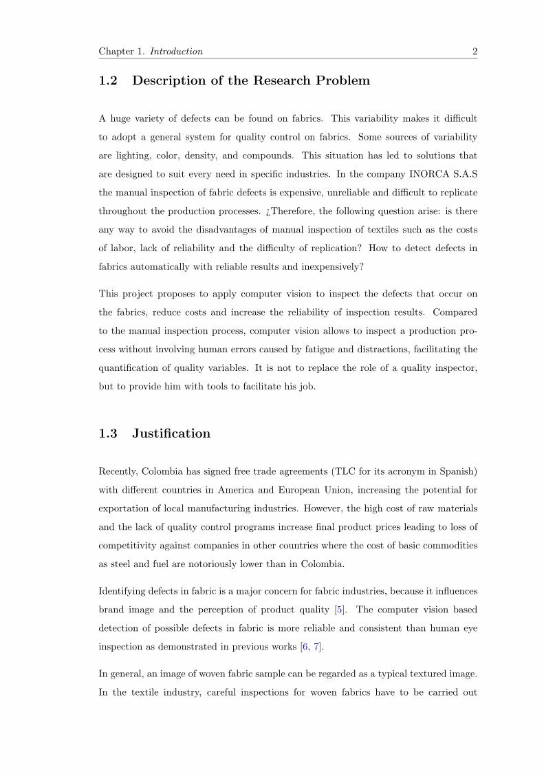
1.2 Description of the Research Problem
A huge variety of defects can be found on fabrics. This variability makes it difficult
to adopt a general system for quality control on fabrics. Some sources of variability
are lighting, color, density, and compounds. This situation has led to solutions that
are designed to suit every need in specific industries. In the company INORCA S.A.S
the manual inspection of fabric defects is expensive, unreliable and difficult to replicate
throughout the production processes. ¿Therefore, the following question arise: is there
any way to avoid the disadvantages of manual inspection of textiles such as the costs
of labor, lack of reliability and the difficulty of replication? How to detect defects in
fabrics automatically with reliable results and inexpensively?
This project proposes to apply computer vision to inspect the defects that occur on
the fabrics, reduce costs and increase the reliability of inspection results. Compared
to the manual inspection process, computer vision allows to inspect a production pro-
cess without involving human errors caused by fatigue and distractions, facilitating the
quantification of quality variables. It is not to replace the role of a quality inspector,
but to provide him with tools to facilitate his job.
1.3 Justification
Recently, Colombia has signed free trade agreements (TLC for its acronym in Spanish)
with different countries in America and European Union, increasing the potential for
exportation of local manufacturing industries. However, the high cost of raw materials
and the lack of quality control programs increase final product prices leading to loss of
competitivity against companies in other countries where the cost of basic commodities
as steel and fuel are notoriously lower than in Colombia.
Identifying defects in fabric is a major concern for fabric industries, because it influences
brand image and the perception of product quality [5]. The computer vision based
detection of possible defects in fabric is more reliable and consistent than human eye
inspection as demonstrated in previous works [6, 7].
In general, an image of woven fabric sample can be regarded as a typical textured image.
In the textile industry, careful inspections for woven fabrics have to be carried out
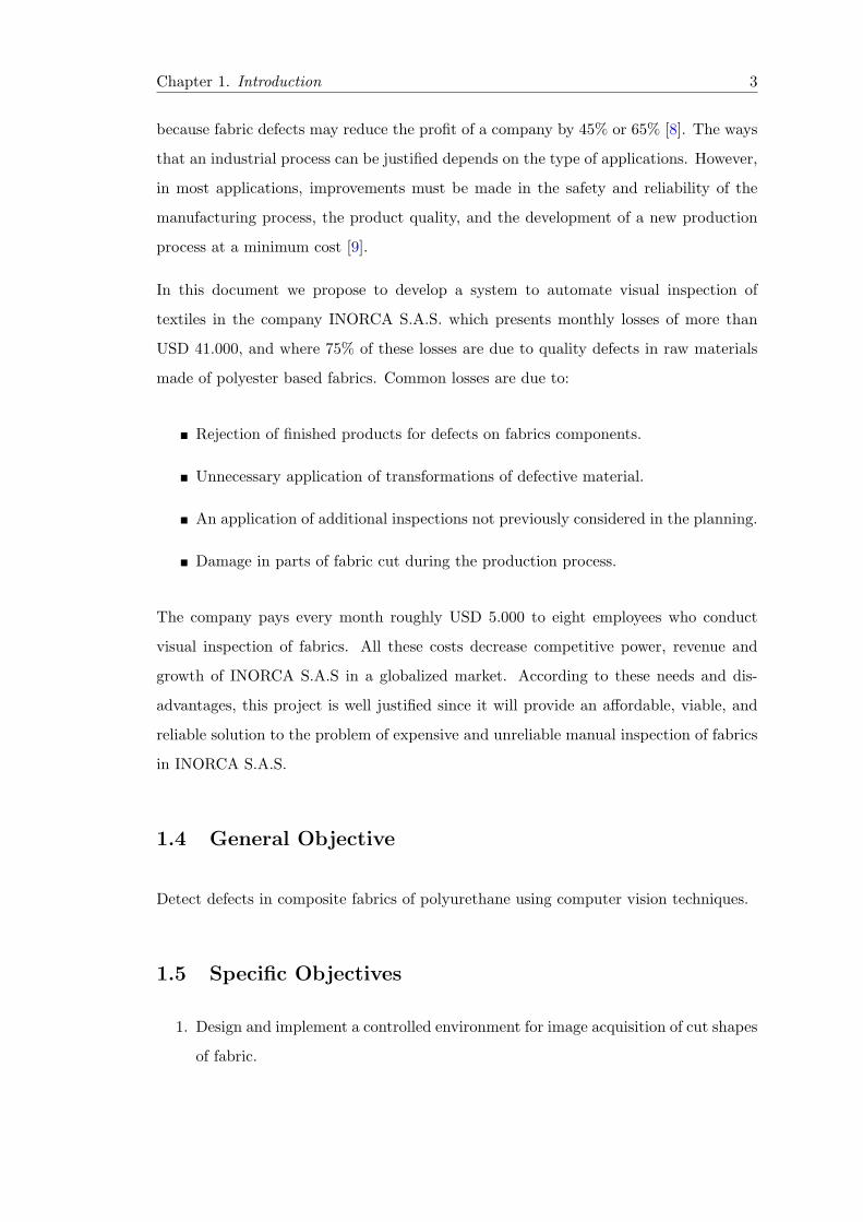
Chapter 1. Introduction 3
because fabric defects may reduce the profit of a company by 45% or 65% [8]. The ways
that an industrial process can be justified depends on the type of applications. However,
in most applications, improvements must be made in the safety and reliability of the
manufacturing process, the product quality, and the development of a new production
process at a minimum cost [9].
In this document we propose to develop a system to automate visual inspection of
textiles in the company INORCA S.A.S. which presents monthly losses of more than
USD 41.000, and where 75% of these losses are due to quality defects in raw materials
made of polyester based fabrics. Common losses are due to:
� Rejection of finished products for defects on fabrics components.
� Unnecessary application of transformations of defective material.
� An application of additional inspections not previously considered in the planning.
� Damage in parts of fabric cut during the production process.
The company pays every month roughly USD 5.000 to eight employees who conduct
visual inspection of fabrics. All these costs decrease competitive power, revenue and
growth of INORCA S.A.S in a globalized market. According to these needs and dis-
advantages, this project is well justified since it will provide an affordable, viable, and
reliable solution to the problem of expensive and unreliable manual inspection of fabrics
in INORCA S.A.S.
1.4 General Objective
Detect defects in composite fabrics of polyurethane using computer vision techniques.
1.5 Specific Objectives
1. Design and implement a controlled environment for image acquisition of cut shapes
of fabric.
Chapter 1. Introduction 4
2. Analyze, select and implement techniques of segmentation, representation, and
classification of digital images that contains cut shapes of fabric.
3. Design a computer vision based inspection system to detect defects in fabrics at
INORCA S.A.S.
4. Validate the performance of the proposed inspection system based on a comparison
with a manual inspection system.
1.6 Project Scope
The scope of this project focuses on the detection of the most costly defects in five types
of fabrics. The classification of fabrics and detection of defects are based on computer
vision. The intended goal for detection rate is 90%.
It is not part of the scope:
� Statistical based predictions.
� Total automation of inspection system.
� Integration with other information systems.
� Generalization of the model for all fabrics and tissues.
1.7 Expected Project Results
� The current detection rate of human inspection is 85%, according to the goal of
INORCA S.A.S the inspection systems proposed is expected to reach at least 90%
of detection performance.
� Design, implementation, and validation of a computer vision based inspection
system to detect defects in cut cloths at INORCA S.A.S.

Chapter 2
THEORETICAL FRAMEWORK
2.1 Previous works and theoretical background.
One of the most important goals of any production process is to consistently deliver
products of high quality. In order to ensure the product quality some form of quality
control needs to be established. Traditionally, the quality control often involves visual
inspection by human operators. Recently, machine vision is being used to automate this
process. An automatic quality control can offer many advantages, such as an increased
productivity and product quality, and the elimination of human errors. Automating the
visual inspection process requires the knowledge of the human operators to be incorpo-
rated into the software [10].
Computer vision allows to the company performing meaningful visual analysis, avoid-
ing destructive and invasive tests and improving the degree of automation of a quality
monitoring system, and thus enhancing both objectivity and repeatability of the mea-
surement/classification process. Successful applications of artificial vision systems range
from process and manufacturing industry, to medical, pharmaceutical, forensic sciences,
and food engineering [11].
Automatic digital image processing and machine vision systems (MVS) have become
increasingly popular because of the ever-decreasing cost of computing power and the
availability and affordability of digital camera systems. MVS is defined as the use of
devices for optical, non-contact sensing to automatically receive and interpret an image of
a real scene in order to obtain information and/or control machines or processes. MVS
5

Chapter 2. Theoretical Framework 6
is now widely accepted and used within the manufacturing industry for applications
including quality assurance and control [12]. The ways that an industrial process can be
justified depends on the type of applications. However; in general, improvements must
be made in the safety and reliability of the manufacturing process, in product quality,
and enabling technology for a new production process at a minimum cost [9].
There are several works in the field of automatic visual inspection and defect detection in
material surfaces. Surveys of existing techniques are provided by Xie (2008) and Kumar
(2008). Due to the wide fields of application (fabric defect detection, surface analysis,
rail inspection, crack detection, among others.) most of these works focus on a specific
problem domain. Among the statistical approaches, gray level statistics (Iivarinen, 2000;
Chetverikov, 2000; Chetverikov and Hanbury, 2002), co-occurrence matrices (Rautkorpi
and Iivarinen, 2005) and local binary patterns (Niskanen et al., 2001; Maenpaa et al.,
2003; Tajeripour et al., 2008) are the most frequently used ones. Unser and Ade, 1984
and Monadjemi et al., 2004 make use of an Eigenfilter approach. Common spectral
methods are Gabor filters (Mandriota et al 2001; Kumar and Pang, 2002), Fourier
analysis (Chan and Pang, 2000) and wavelet-based approaches (Serdaroglu et al., 2006).
Model-based approaches often model the stochastic variations of a surface with help
of Markov random fields (Cohen et al., 1991). Due to the lack of defective training
samples anomaly detection (Chandola et al., 2009; Markou and Singh, 2003a; Markou
and Singh, 2003b), one-class classification (Tax, 2001) and outlier detection (Hodge and
Austin, 2004) are relevant concepts (Tajeripour et al., 2008; Xie, 2008) [13].
Textile fault detection has been studied using various approaches; one approach (Sari-
Sarraf and Goddard, 1999) uses a segmentation algorithm, which is based on the concept
of wavelet transform, image fusion and the correlation dimension. The essence of this
segmentation algorithm is the localization of defects in the input images that disturb
the homogeneity of texture. Another approach presented in (Daul et al., 1998) consists
of a preprocessing step to normalize the image followed by a second step of associating a
feature to each pixel describing the local regularity of the texture and localize defective
pixels [14].
The development of real-time automated visual fabric inspection systems, in general,
consists of three processes, namely, image acquisition, image processing, and image

Chapter 2. Theoretical Framework 7
analysis. Typical examples include Elbit Vision Systems I-TEX system [15], BarcoVi-
sion’s Cyclops[16] and Zellweger Uster’s Fabriscan [17]. These systems inspect fabric in
full width at the output of a finishing machine. They are designed to find and catalog
defects in a wide variety of fabrics including greige fabrics, sheeting, apparel fabrics,
upholstery fabrics, industrial fabrics, tire cord, finished fabrics, piece-dyed fabrics and
denim. However, they cannot inspect fabrics with very large and complex patterns.
Other examples include a fuzzy wavelet analysis system for process control in the weav-
ing process, a vision system for on loom fabric inspection, a vision system for on-circular
knitting machine and a vision system for fabric detection based on different Gabor fil-
ters. These systems are rather expensive which prevent them from being widely adopted
by small to medium sized factories [18].
Texture analysis has various applications in different areas on computer vision, image
processing, medical image processing and related fields. There is no clear-cut definition
for image texture. Image texture is believed to be a rich source of visual information –
about the nature and 3D shape of physical objects (Materka and Strzelecki, 1998). Tex-
tures are complex visual patterns composed of entities, or sub-patterns – that have char-
acteristic brightness, color, slope, size, among others. Hence, texture can be regarded
as a similarity grouping in an image (Rosenfeld and Kak, 1982). The local sub-pattern
properties give rise to the perceived lightness, uniformity, density, roughness, regularity,
linearity, frequency, phase, directionality, coarseness, randomness, fineness, smoothness,
granulation, among others, of the texture as a whole (Materka and Strzelecki, 1998).
In another definition, the texture of images refers to the appearance, structure and ar-
rangement of the parts of an object within the image (Castellano et al., 2004). Smarter
extraction of features from image textures produce better cues for image analysis, which
are pivotal for object recognition, surface analysis, action recognition, disease diagno-
sis, among others. There are various approaches for texture analysis. Most of these
approaches are based on structural, model-based, statistical (e.g., histogram, absolute
gradient, run-length matrix, co-occurrence matrix, auto-regressive model, wavelets) [19].
In [20] Mahajan, Kolhe and Patil propose an important starting point to classify the
approaches used so far in the representation of defects on fabrics. These approaches are
statistical, spectral, and model based which are described below.
Chapter 2. Theoretical Framework 8
2.1.1 Statistical Approaches
Statistical texture analysis methods measure the spatial distribution of pixel values.
An important assumption in this approach is that the statistics of defects free regions
are stationary, and these regions extend over a significant portion of inspected images.
The first-order statistics estimate properties like the average and variance of individual
pixel values, ignoring the spatial interaction between image pixels. Second and higher
order statistics estimate properties of two or more pixel values occurring at specific
locations relative to each other. The defect detection methods employing texture features
extracted from fractal dimensions, first order statistics, cross correlation, edge detection,
morphological operations, co-occurrence matrix, eigenfilters, rank order functions, and
many local linear transforms have been categorized into this class [20].
2.1.2 Spectral Approaches
In spectral based approaches texture is characterized by texture primitives or texture
elements, and the spatial arrangement of these primitives. Thus, the primary goals
of these approaches are firstly to extract texture primitives, and secondly to model or
generalize the spatial placement rules. The high degree of periodicity of basic texture
primitives, such as yarns in the case of textile fabric, allows the usage of spectral features
for the detection of defects. However, random textured images cannot be described in
terms of primitives and displacement rules as the distribution of gray levels in such
images is rather stochastic. Therefore, spectral approaches are not suitable for the
detection of defects in random texture materials. Various approaches for the detection
of defects in uniform textured material using frequency and spatial-frequency domain
features have been reported in the literature. In spectral-domain approaches, the texture
features are generally derived from the Fourier transform, Gabor transform and Wavelet
transform [20].
2.1.3 Model-Based Approaches
Model - based texture analysis methods are based on the construction of an image model
that can be used not only to describe texture, but also to synthesize it. Model-based
approaches are particularly suitable for fabric images with stochastic surface variations

Chapter 2. Theoretical Framework 9
(possibly due to fiber heap or noise) or for randomly textured fabrics for which the sta-
tistical and spectral approaches have not yet shown their utility. The model parameters
capture the essential perceived qualities of texture. Markov random fields (MRF) have
been popular for modeling images. MRF theory provides a convenient and consistent way
for modeling context dependent entities such as pixels, through characterizing mutual
influences among such entities using condition MRF distribution. Several probabilistic
models of the textures have been proposed and used for defect detection; Cohen (1991)
used Gaussian Markov Random Fields (GRMF) to model defect free textile web. The
inspection process was treated as a hypothesis testing problem on the statistics derived
from the GMRF model. The images of fabric to be inspected are divided into small win-
dows in inspection process. A likelihood ratio test is then used to classify the windows
as non– defective or defective. The testing image is partitioned into non-overlapping
sub-blocks where each window was then classified as defective or non-defective [20].
Previous works show two fabric defect detection approaches. One is based on transform
domain like Gabor filters and another hinges on statistical texture analysis like Gray
Level Co-occurrence Matrix (GLCM). However few other versions of these models and
different models are also available. Karayiannis (1999) presented multi-resolution de-
composition based real time fabric defect detection system (FDDS). Cohen (1991) has
characterized the fabric texture using the Gauss Markov random field (GMRF) model
and the fabric inspection process is treated as a hypothesis-testing problem on the statis-
tics derived from this model and classifying textile faults with a back-propagation neural
network using power spectrum. Zuo (2012) used NL-means filtering algorithm for tex-
ture enhancement where GLCM was used with Euclidean distance to find defects. He
showed overall detection rate of 88.79%. Siew has shown assessment of carpet wear using
spatial gray level dependence matrix (SGLDM) [8].
The most commonly used features are the second-order statistics derived from spatial
gray-level co-occurrence matrices. The fabric texture exhibits a high degree of period-
icity, and thus Fourier-based methods characterize the spatial-frequency distribution of
textured images, but they do not consider the information in the spatial domain and
may overlook local deviations [8].
Defect detection, which interests quality inspection, separates products into two main
Chapter 2. Theoretical Framework 10
classes, acceptable if there is no defect in product and not acceptable if there is any de-
fect. In contrast, defect classification determines which kind of defect has been occurred.
It could help maintenance personnel to spot the type of needed repairing of product line.
Defect detection could be considered as a specific case of defect classification and two
tasks are basically similar in most practical steps including image acquisition, prepro-
cessing, feature extraction and arithmetic operations for inferring and decision making
[21].
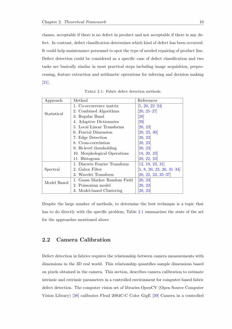
Table 2.1: Fabric defect detection methods.
Approach Method References
Statistical
1. Co-occurrence matrix [5, 20, 22–24]2. Combined Algorithms [20, 25–27]3. Regular Band [28]4. Adaptive Dictionaries [29]5. Local Linear Transforms [20, 23]6. Fractal Dimension [20, 23, 30]7. Edge Detection [20, 23]8. Cross-correlation [20, 23]9. Bi-level thresholding [20, 23]10. Morphological Operations [18, 20, 23]11. Histogram [20, 22, 23]
Spectral1. Discrete Fourier Transform [12, 19, 23, 31]2. Gabor Filter [5, 8, 20, 23, 26, 31–34]3. Wavelet Transform [20, 22, 23, 35–37]
Model Based1. Gauss Markov Random Field [20, 23]2. Poissonian model [20, 23]3. Model-based Clustering [20, 23]
Despite the large number of methods, to determine the best technique is a topic that
has to do directly with the specific problem, Table 2.1 summarizes the state of the art
for the approaches mentioned above
2.2 Camera Calibration
Defect detection in fabrics requires the relationship between camera measurements with
dimensions in the 3D real world. This relationship quantifies sample dimensions based
on pixels obtained in the camera. This section, describes camera calibration to estimate
intrinsic and extrinsic parameters in a controlled environment for computer-based fabric
defect detection. The computer vision set of libraries OpenCV (Open Source Computer
Vision Library) [38] calibrates Flea3 20S4C-C Color GigE [39] Camera in a controlled

Chapter 2. Theoretical Framework 11
environment. This section also presents the design, implementation and testing of the
controlled environment for image acquisition.
Camera calibration is a necessary step in automatic inspection of fabric defects to ex-
tract metric information from 2D images. It provides a model of camera geometry and
distortion model of the lenses, Tables 2.2 and 2.3 summarize the components involved
in the calibration, the specific reason for using this camera is the speed of transmission
with GigE connection and representation capacity obtained with the combination of
lens/sensor. Figures 2.1 and 2.2 show the camera and the lens deployed in this work.
The calibration process is based on pinhole camera model in which, a single ray of light
enters the camera from the scene or a distant object to be projected on an imaging
surface.
Table 2.2: Hardware
Lens 6 mm Compact fixed focal length
Connection Cat 5e GigE cable, RJ45 type
Power Supply Universal Power Supply and GPIO Leads
Table 2.3: Camera specifications
Model Number FL3-GE-20S4C-C
Camera Sensor Format 1/1.8”
Imaging Device Progressive Scan CCD
Type of Sensor Sony ICX274
Pixels (H x V) 1624 x 1224
Pixel Size, H x V (µ m) 4.4 x 4.4
Frame Rate (fps) 15
Figure 2.1: Point Grey - Flea3 FL3-GE-20S4C-C Camera.
In consequence, the size of the image projected on the projective plane is controlled by
camera’s focal length. For our idealized pinhole camera, the distance from the pinhole
aperture to the screen is precisely the focal length. Figure 2.3 presents this model, where

Chapter 2. Theoretical Framework 12
Figure 2.2: Edmunds Optics - 6 mm Compact Fixed Focal Length Lens.
f is the focal length of the camera, Z is the distance from the camera to the object, X is
the length of the object, and x is the object’s image on the imaging plane.
Figure 2.3: Pinhole model with identification of key variables
2.2.1 Image Formation
The relation that maps the point Pi into the physical world with coordinates q =
(xi, yi, zi) to the point on the projection screen with coordinates u, v is called projective
transform.
Parameters that define the camera such as (fx, fy, cx, and cy) are intrinsic. Where fx
and fy are focal lengths in x and y directions. cx and cy represent a possible displace-
ment (away from the optic axis) of the center of coordinates on the projection screen.
Extrinsic parameters relate the object’s position relative to the camera coordinate sys-
tem in terms of rotation and translation matrices.

Chapter 2. Theoretical Framework 13
2.2.2 Homogeneous coordinates
The homogeneous coordinates of a point in three dimensions represented in Cartesian
coordinates (X,Y, Z)T are defined as the point (kX, kY, kZ, k)T where k is an arbitrary
constant different to 0. A point P of the real-world space represented by Cartesian
coordinates can be expressed in a vector form as [1]:
P =
X
Y
Z
In homogeneous coordinates:
Ph =
kX
kY
kZ
k
2.2.3 Perspective projection
As indicated above the projection perspective explains the formation of images in a
camera whose functional model is represented by the pinhole model. Figure 2.4 shows
the formation of an image using the perspective projection. Rw is the coordinate system
of the world where object of interest is located, Rc is the coordinate system centered at
the optical center of the camera, and Ri is image coordinates.
Points in the real world are represented on a three dimensional basis, while points
on the image are two dimensional. The relation that maps points Qi in the physical
world represented with coordinates (Xi, Yi, Zi) to the points on the projection screen
with coordinates (xi, yi) is called a projective transform. The homogeneous coordinates
associated with a point Q in the projective space of dimension n are typically expressed
as an (n+1) dimensional vector (e.g., x, y, z becomes x, y, z, w). Clearly the optical axis
is aligned with the Z axis of the reference system of the camera. The center of the image
plane coincides with the origin of both systems, in which Z axis loses importance for
model reference since it becomes a constant value.

Chapter 2. Theoretical Framework 14
(x) (X)
( , , )X Y Z
{ }Rw
{ c}R
(y) ( )Y
Image plane
(x,y)
focal distance
(z) (Z)
Figure 2.4: Modeling perspective projection [1]
In this work, the image plane corresponds to the projective space and it has only
two dimensions, so we will represent points on that plane as three-dimensional vec-
tors q = (q1, q2, q3). All points having proportional values in the projective space are
equivalent, division by q3 recovers the actual pixel coordinates. This allows us to arrange
the parameters that define our camera (i.e., fx, fy, cx, and cy) into a single 3-by-3 ma-
trix, which we will call the camera intrinsics matrix parameters (the approach used by
OpenCV compute to camera intrinsics is derived from Heikkila and Silven [Heikkila97]).
Let’s supposse a point in space with coordinates Mc = (Xc, Yc, Zc)T , and its correspond-
ing image coordinates mi = (xi, yi), Zc > f , indicates that the points of interest are
located in front of the camera. Figure 2.5 shows the relationship between world and
image coordinates by triangle similarity.
Figure 2.5: Relationship between world and image coordinates.

Chapter 2. Theoretical Framework 15
xif
= − Xc
Zc − f=
Xc
f − Zc⇒ xi =
fXc
f − Zc(2.1)
yif
= − YcZc − f
=Yc
f − Zc⇒ yi =
fYcf − Zc
(2.2)
Then
m =
x
y
=
fXc
f−Zc
fYc
f−Zc
(2.3)
The first two components are the coordinates m(x, y) in the image plane of the three-
dimensional point (X,Y, Z) projected. As mentioned above, the third component, z, is
constant in this plane. In the Figure 2.3 the negative sign in front of Xc and Yc indicates
that the image is inverted. These equations are nonlinear because they contain a division
by Zc. For geometric transformations it is suitable to express these expressions in matrix
form by converting them into homogeneous coordinates. The homogeneous coordinates
of the point are Mch = (KXc,KYc,KZc,K)T where K is an arbitrary nonzero constant.
Mih is an image point in homogeneous coordinates. Defining B as a perspective matrix
that relates the points of space with the image points in homogeneous coordinates.
B =
1 0 0 0
0 1 0 0
0 0 −1f 1
BMch = mh
1 0 0 0
0 1 0 0
0 0 −1f 1
∗
kXc
kYc
kZc
k
=
kXc
kYc
k(
f−Zc
f
)

Chapter 2. Theoretical Framework 16
2.2.4 Homogeneous transformation
So far the coordinate system of the camera coincides with the world, i.e the experimental
platform where the fabric to be inspected. A more general case involves a transforma-
tion that converts the world coordinates Rw into the camera Rc coordinates as seen in
Figure 2.6.
Z
{ }Rw
Y
X
{ }Rc
Camera
x
y
z
Figure 2.6: Final position (translation and rotation)
To obtain the complete pinhole camera model it is necessary to scale and translate the
image. Scaling occurs in a rectangular grid with dy scale factors in the vertical direction
and dx in the horizontal direction, the angle between the x axis and the y axis is defined
by the skew coefficient, which is only equal to zero if the angle is positive.
The following steps must be followed to transform the camera coordinate system into
world coordinate system:
1. Rotation around the x axis with angle α
2. Rotation around the y axis by an angle β
3. Rotation around the z axis with angle θ
The translation is represented by (x0, y0). The values x∗i and y∗i are the coordinates of
the point after applying the central projection, being xi, yi the coordinates in the system
image, they are listed according to the following equations:
{xi = x0 + dxx∗i } (2.4)
Chapter 2. Theoretical Framework 17
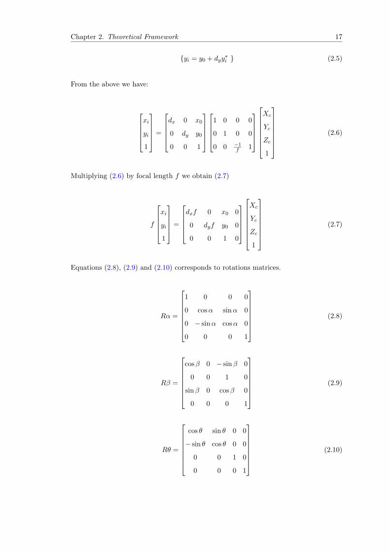
{yi = y0 + dyy∗i } (2.5)
From the above we have:
xi
yi
1
=
dx 0 x0
0 dy y0
0 0 1
1 0 0 0
0 1 0 0
0 0 −1f 1
Xc
Yc
Zc
1
(2.6)
Multiplying (2.6) by focal length f we obtain (2.7)
f
xi
yi
1
=
dxf 0 x0 0
0 dyf y0 0
0 0 1 0
Xc
Yc
Zc
1
(2.7)
Equations (2.8), (2.9) and (2.10) corresponds to rotations matrices.
Rα =
1 0 0 0
0 cosα sinα 0
0 − sinα cosα 0
0 0 0 1
(2.8)
Rβ =
cosβ 0 − sinβ 0
0 0 1 0
sinβ 0 cosβ 0
0 0 0 1
(2.9)
Rθ =
cos θ sin θ 0 0
− sin θ cos θ 0 0
0 0 1 0
0 0 0 1
(2.10)

Chapter 2. Theoretical Framework 18
Since the translation matrix must be concatenated with other rotation matrices it is
convenient to convert it into a square matrix using (2.11).
Tr =
1 0 0 rx
0 1 0 ry
0 0 1 rz
(2.11)
Where rx, ry and rz are the translation components in x, y, z, and Tr represents the
translation matrix. Rα , Rβ and Rθ are rotation matrices around angles α, β and θ,
respectively.
x∗
y∗
z∗
=
1 0 0 rx
0 1 0 ry
0 0 1 rz
x
y
z
1
→
x∗ = x+ rx
y∗ = y + ry
z∗ = z + rz
(2.12)
Final integration of rotation matrix is:
R =
cosβ cos θ cosβ sinα − sinβ 0
sinα sinβ − cosα sinβ sinα sinβ sin θ + cosα cosβ sinα cosβ 0
cosα sinβ cos θ − sinα sinβ cosα sinβ cos θ − sinα sinβ cosα cosβ 0
0 0 0 1
(2.13)
The composition of the translation and rotation results in matrix E shown in (2.14).
E =
R Tr
0T 1
(2.14)
Appendix B presents the experimental configuration. Camera’s optic axis is parallel to
surface’s normal vector on which the fabric sample will be placed.
2.2.5 Camera parameters
2.2.5.1 Intrinsic parameters
Camera intrinsic parameters depends on factors such as focal length, CCD (Charge-
Coupled Device) dimension, and lens distortion. Heikkila[97] defines the effective focal

Chapter 2. Theoretical Framework 19
length f, scale factor s, and the image center (u0, v0) also called the principal point as
intrinsic parameters. Equation (2.7) permits to find these parameters as:
fx = dxf (2.15)
fy = dyf (2.16)
cx = x0 (2.17)
cy = y0 (2.18)
xscreen = fx
(
X
Z
)
+ cx (2.19)
yscreen = fy
(
Y
Z
)
+ cy (2.20)
The focal lengths fx and fy are different since the individual pixels on a typical low-cost
imager are rectangular rather than square. The focal length fx is actually the product
of the physical focal length of the lens and the size sx of the individual imager elements.
Generally the center of the sensor is not in the optical axis. Therefore parameters, cx
and cy are used to model possible shift (distance from the optical axis) of the center
coordinates in the projection screen. The result is a relatively simple model in which a
point Q in the physical world, with coordinates (X,Y, Z) is projected on the screen at
any given pixel location (Xscreen, Yscreen).
2.2.5.2 Extrinsic parameters
As opposed to the intrinsic parameters that describe internal parameters of the camera
(focal distance, radial lens parameters), the extrinsic parameters indicate the exter-
nal position and orientation of the camera in the 3D world. Camera extrinsic matrix
describes the transformation of world coordinates into camera coordinates, Figure 2.7
shows the information flow from real-world coordinates to camera coordinates (i.e from
3D to 2D).
Extrinsic parameters consists of three components:
1. Translational component Tx, Ty, Tz; seen before in equation 2.11

Chapter 2. Theoretical Framework 20
2. Distance component (camera optical center).
3. Rotation component Rα, Rβ, Rθ seen in equations 2.8, 2.9 and 2.10 respectively.
Object Coordinates 3D
World Coordinates (3D)
Camera Coordinates 3D
Image Plane Coordinates (2D)
Pixel Coordinates (2D)
}}
extrinsic cameraparameters
intrinsic cameraparameters
Figure 2.7: Order of applying parameters from the real world to the camera
2.2.6 Lens distortions
The estimation of object’s size is an important task in optical measurement. Lens distor-
tion affects its performance. This study characterizes radial and tangential distortions
in the lenses that conform the computer vision based measurement system. Figure 2.8
shows a type of distortion known as the barrel distortion by deformations in the edges
of the image, a defect is clearly associated with the lens.
lens
Image PlaneO jectb
Radial Distortion
Figure 2.8: Example of radial distortion (barrel distortion). [2]
2.2.6.1 Radial distortion
The lenses of real cameras often noticeably distort the location of pixels near the edges
of the imager. This phenomenon is the origin of the barrel or fish eye effect. Figure 2.8
illustrates the reasons of radial distortion. With some lenses, rays farther from the center

Chapter 2. Theoretical Framework 21
of the lens are bent more than those closer in. The parameters associated with the radial
distortion are named as k1 and k2.
For radial distortion, the distortion is 0 at the (optical) center of the imager and in-
creases as we move toward the periphery. In practice, this distortion is small and can
be characterized by the first few terms of a Taylor series expansion around r = 0. For
low-cost web cameras, we generally use the first two terms; the first called k1 and the
second is k2. In general, the radial location of a point on the imager will be rescaled
according to the following equations:
xrcorrected = x(1 + k1r2 + k2r
4 + k3r6) (2.21)
yrcorrected = y(1 + k1r2 + k2r
4 + k3r6) (2.22)
Here (x, y) is the original location (on the imager) of the distorted point and (xrcorrected, yrcorrected)
is the new location as a result of the correction.
2.2.6.2 Tangential distortion
The second-largest common distortion is tangential distortion. This distortion is due to
manufacturing defects resulting from the lens not being exactly parallel to the imaging
plane. Tangential distortion is minimally characterized by two additional parameters p1
and p2, such that:
xtcorrected = x+ [2p1y + p2(r2 + 2x2)] (2.23)
ytcorrected = y + [p1(r2 + 2y2) + 2p2x] (2.24)
Thus in total there are five distortion coefficients that we require. Because all five are
necessary in most of the OpenCV routines that use them, they are typically bundled
into one distortion vector; this is a 5× 1 matrix containing k1, k2, p1, p2, and k3.
2.3 Illumination systems
Illumination plays an important role in the development of computer vision based in-
spections, whether automated or manual. The presence of shadows negatively impacts

Chapter 2. Theoretical Framework 22
the performance of segmentation and classification algorithms. Table 2.4 describes the
amount of light recommended to carry out different activities that require the visual
attention. The average luminance is given by:
Lum =LuminousF lux× Utilizationfact×Maintenancefact
(area)m2 (2.25)
Table 2.4: Preferred sustained luminance levels for different locations or visual tasks- Encyclopedia of health and safety at work [3].
Task/Location Recommended LuxOffice 500Computerized workstations 500Manufactures mounting areas 500Low precision work 300Medium accuracy work 500Precision work 750Assembling Instruments 1000Installation and repair of jewelry 1500Operating rooms 50000
The criteria taken into account to define the type of illumination are:
1. Luminance provided by the source must be equal or greater than the illumination
required by a human to execute high precision task that requires visual attention.
2. Durability of at least one year.
3. Adaptivity to several heights and orientations with respect to the inspected surface.
4. Operation voltage ranging from 110V to 220V.
It’s difficult to find information about lighting configurations for fabrics inspection. How-
ever, by taking into account the requirements described above, an array of tubular lamps
with LED technology was selected. Table 2.5 shows technical facts of this bulb provided
by the manufacturer [40].
Each tubular bulb has a length of 1.20 m (as shown in Figure 2.9). Based in pinhole
model calculate the lighting coverage in the scene that contains the fabric sample to be
inspected, the illumination set-up is made of two bulbs, at a distance (h) of 1.18 m from
the table to the lamps. This configuration provides an illuminated region on the table

Chapter 2. Theoretical Framework 23
Table 2.5: Information provided by the manufacturer of T8 LED Tube 22W.
Item ValueNominal power 22WNominal voltage 110-220V.Nominal Electrical Current 290 mA.Lumen flux 2250 lumensMaintenance factor 0.65Standard IEC 60968Projection Angle 80◦
of sizes 1.678 m and 0.7031 m, with a luminance of 1463 lux.
tan(80/2) =Area
1
Area = tan(40)× 1 m× 2
Area = 1, 678 m2
Figure 2.9: Tubular bulb, T8 led 22W - 1.20 m.
The above calculation provides an important hint to determine the appropriate distances
between the fabric and the illumination source. This means that to attain an illuminated
area with 1.678 m2 wide the lamps must be placed at a minimum height (h) of 1.18 m.
That is:
tan(80/2) = (h/2)/xMax
tan(80/2) = (1.18 m/2)/xMax
xMax = 0.7031 m.
Where xMax is the height of the effective surface. The illumination set-up contains two
tubes spaced by 10 cm.
2.4 Fabrics and selection of defects
Segmentation of a given defect with prior knowledge of its shape, size or distribution is
known as supervised defect segmentation. For the scope of the present work, we selected
five types of fabrics with defects. Table 2.6 shows the main defects presented in fabrics at
INORCA company, between January and September 2013, this analysis includes 97.9%

Chapter 2. Theoretical Framework 24
of all defects. The remaining 2.91% corresponds to defects that occur with an individual
percentage less than 0.01%, thus this ranking does not consider them.

Chapter 2. Theoretical Framework 25
2.4.1 Main defects ranking
Table 2.6: Ranking of the main defects on fabrics occurred between January andSeptember 2013 detected by human inspection
Fabric defect cost in US DollarsFabric Cost by defect
# Continuity Scratch No-cont LF CF SF DT. Total %tissue
1 Kariatyde 495 3.509 9.237 0 4.289 0 0 17.530 22.49
2 Vulcron vinyl W/L 0 9.084 0 0 5.845 0 137 15.066 19.33
3 Vulcron vinyl N/L 0 6.154 0 0 5.284 0 0 11.438 14.67
4 Petit point gray 0 4.878 0 0 4.734 0 0 9.611 12.33
5 Petit point red 0 5.740 420 159 0 0 0 6.319 8.11
6 Baltic vinyl 0 0 0 0 2.545 0 176 2.722 3.49
7 Geneva 0 1.672 38 46 0 0 836 2.592 3.32
8 Craquele 268 1.443 0 0 60 0 0 1.771 2.27
9 Pliss 0 1.181 0 0 0 0 409 1.590 2.04
10 Roseau 77 1.164 0 328 0 0 0 1.568 2.01
11 Kario carbone 0 443 0 0 703 0 0 1.145 1.47
12 Baji 0 1027 0 0 0 0 0 1.027 1.32
13 Kario black normal 0 76 412 0 445 0 0 933 1.20
14 Perle copo 0 495 189 0 17 0 0 701 0.90
15 Kario orange 0 309 0 0 358 0 0 667 0.86
16 Corsario Billiard 0 0 0 0 185 296 0 481 0.62
17 Poesy mod copo 0 416 16 0 0 0 0 432 0.55
18 Kario black LG 2 mm 0 143 32 0 127 0 0 302 0.39
19 Duo carbon fonce 0 180 0 0 69 0 0 249 0.32
21 Demo blue 0 99 21 0 0 0 0 120 0.15
22 No-woven unspecific 0 0 0 0 25 25 0 50 0.06
23 Embossed GT Line 1 0 3 0 1 0 0 5 0.006
Total 840 39.353 10.369 533 24.984 320 1.159 77.958 97.90
2.4.2 Defects criteria selection
Based on the analysis of financial costs generated by defects in different types of fabrics,
a total of five fabrics types are selected to be detected as listed in Table 2.7. From these
fabrics two defects were analyzed; a defect for each type of fabric. However it is possible
that on the same fabrics other defects may occur. Next part describes the appearance
of selected defects.
Continuity : corresponds to problems caused by incorrect splicing fabrics
Scratch: corresponds to the marks made by operators on fabrics indicating that in these
places there may be problems, operators mark with pen if the fabric is a white synthetic
surface or with white chalk in case it is a woven fabric. Commonly, these strokes may
be difficult to identify by operators due to long work operation hours. Figures 2.11e and
2.11c illustrates the default scratch in a synthetic fabric and a woven fabric respectively.

Chapter 2. Theoretical Framework 26
Table 2.7: Main defects selected under the criterion of the highest cost
Fabric defect cost in US DollarsFabric Cost by defect
# Fabric Continuity Scratch Noncontinuous LF CF SF DT Total %tissue
1 Kariatyde 9.237 9.237 11.85
2 Vulcron vinyl W/L 9.084 9.084 11.65
3 Vulcron vinyl N/L 6.154 6.154 7.89
4 Petit point gray 4.878 4.878 6.26
5 Petit point red 5.740 5.740 7.36
Total 0 25.856 9.237 45.02
Noncontinuous tissue: is the lack of a thread in the sequence of tissue and usually
appears as a dotted straight line as seen in Figure 2.11a, this type of defect usually has
a width of 0.2 and 0.5 mm.
LF : lamination failure: are errors in the laminate process of fabrics.
CP : crumpled piece: are caused by failures in the treatment of fabrics.
SF : stained fabric: are caused by failures in the treatment of fabrics.
DH : differences in tones: are caused by faults in the manufacturing process of the fabrics.

Chapter 2. Theoretical Framework 27
(a) Karyatide. (b) Gray petit.
(c) Red petit.
(d) Vulcron vinyl WL. (e) Vulcron vinyl NL.
Figure 2.10: Selected fabric images

Chapter 2. Theoretical Framework 28
(a) Karyatide - noncontinuous tissue. (b) Gray petit - scratch.
(c) Red petit - scratch.
(d) Vulcron vinyl WL - scratch.1
1 defect located on the left side(vertical).
(e) Vulcron vinyl NL - scratch2
2 defect located on the center(diagonal).
Figure 2.11: Selected images of defective fabrics.
Chapter 3
DEFECT DETECTION AND
FABRICS REPRESENTATION
3.1 Defect detection in fabrics
After calibrating the camera, and selecting the types of fabrics and defects to be clas-
sified, it’s very important to determine a strategy to segment the defects in an image.
In this work, we select Gabor filters as a representation for defect segmentation in three
fabrics types (kariatyde, petit-point gray and petit-point red). Simple thresholding seg-
ments two fabrics: Vulcron Vinyl WL and Vulcron Vinyl NL. The surfaces of these
fabrics do not present a specific orientation; hence Gabor filtering is not a suitable for
their representation.
3.1.1 Gabor filters
Multichannel Gabor filters are a joint spatial/spatial-frequency representation for an-
alyzing textured images with highly specific frequency and orientation characteristics.
This technique extracts features by filtering the textured image with a set of Gabor filter
banks characterized by the frequency, the orientation of the sinusoid, and the scale of
the window function [27].
29

Chapter 3. Defect detection and fabrics representation 30
The transform of Gabor was initially defined by Gabor in [41] and extended by Daugman
in [42]. The Gabor filter is in practice a linear filter whose impulse response is a sinusoidal
function multiplied by a Gaussian function.
The application of the of Gabor filters is provided by a bank of filters with size M ×N ,
where M is the number of dilations and N is the number of rotations, G Daugman
(2002) found that the response of simple cells in the visual cortex of the mammalian
brain can be modeled by Gabor functions. Therefore, the image analysis by Gabor
functions is similar to the human visual perception system. The Gabor filter bank has
been extensively studied in visual inspection. Kumar and Pang (2000) perform fabric
defect detection using only real Gabor functions. Later in 2002, they used a class of self
similar Gabor functions to classify fabric defects [20].
Gabor filters decomposes images into different scales and orientations hence they may
highlight defects in fabrics. Gabor filter for fabric defect detection has good perfor-
mances both in spatial domain and in frequency domain. In general, an even symmetric
Gabor filter is good at detecting blob-shaped fabric defects, while an odd symmetric one
performs well in detecting edge-shaped fabric defects. In this method, even symmetric
and odd symmetric Gabor filter masks are used for better defect detection [8].
As mentioned earlier, in the spatial domain, the Gabor function is a complex exponen-
tial modulated by a Gaussian function. The Gabor function forms a complete but a
nonorthogonal basis set and its impulse response in the two–dimensional (2-D) plane
has the following general form [41]:
f(x, y) =1
2πσxσy
[
− 12
(
x2
σ2x
+ y2
σ2y
)](2πju0x)
(3.1)
Where u0 denotes the radial frequency of the gabor function, σx and σy define the
Gaussian envelope along the x and y axis. Figure 3.1 shows the perspective plot of a
typical Gabor filter in the spatial domain.
In the frequency domain, the Gabor function acts as a bandpass filter and the Fourier
transform of f(x, y)is given by:
F (u, v) = exp
{
−1
2
[
u− u20σ2u
+v2
σ2v
]}
(3.2)

Chapter 3. Defect detection and fabrics representation 31
Figure 3.1: Components of a Gabor function in spatial domain.
where
σu =1
2πσxand σv =
1
2πσy
Using (3.1) as the mother Gabor wavelet, the self-similar filter bank can be obtained by
appropriate dilation and rotation of the generating function:
fp,q = α−P f(x′, y′) (3.3)
where
x′ = α−P (x cosθq + y sin θq)
= α−P (−x sin θq + y cos θq)
α > 1 p = 1, 2, ..., S;q = 1, 2, ..., L.

Chapter 3. Defect detection and fabrics representation 32
The integer subscripts p and q represent the index for scale (dilation) and orientation
(rotation), respectively. S is the total number of scales and L is the total number of
orientations in the self-similar Gabor filter bank. For each orientation q the angle θq is
given by:
θq =π(q − 1)
L, q = 1, 2, ..., L. (3.4)
The scaling factor α−P ensures that the all energy image Epq =∫ −∞
∞
∫ −∞
∞|fpq(x, y)|2 dxdy
is independent of p [43]. Thus, all the filters in the Gabor filter bank have the same
energy, irrespective of their scale and orientation.
This work is centered on asymmetric Gabor filters, this mean σx 6= σy; asymmetric
Gabor filters can be useful for real fabric textures, Gabor function does not exactly
satisfy the requirements that the wavelet be admissible and progressive [43]. However,
in the context of representing a class of self-similar functions, this term is used. The
following formulas ensure that the half-peak magnitude responses of adjacent asymmetric
filters touch each other [34]:
α =
(
θhθ
)
α−P =
(
θhθ
)−( 1(s−1)
)
σx =
√2 ln 2(α+ 1)
2πσxθh(α− 1)
thus,
σy =
[
2 ln 2−(
2 ln 2
2πσxθh
)2]1/2
[
2π tan( π
2L
)
(
θh − 2 ln 2
(
1
4π2σ2xθh
))]−1(3.5)
where u0 = θh, while θl and θh are the lowest and highest frequencies. A bank of self-
similar Gabor filters formed by rotation (varying q) and dilation (varying p) is used to

Chapter 3. Defect detection and fabrics representation 33
perform power spectrum sampling of the inspection images.
Each of the Gabor filters value has the real part (even) and imaginary part (odd), that
are conveniently implemented as the spatial mask of M ×M sizes. In order to have a
symmetric region of support M is preferred to be an odd number. For a given input
image I(x, y) the magnitude of filtered image Ipq(x, y) is obtained by using Gabor filter
fpq(x, y) as follows:
Ipq(x, y) ={
[fpq(x, y)e ∗ I(x, y)]2 + [fpq(x, y)o ∗ I(x, y)]2}1/2
(3.6)
where ”*” denotes 2-D convolution operation, and fpq(x, y)e and fpq(x, y)o represent the
even and odd parts of the Gabor filter separated from (3.4)
Gabor filter analysis provides an image for each pair of orientation and scale values.
Gabor filters outputs reveal the orientations and scales of defects in the fabrics with
defined textured patterns. Although there is a limited amount of a priori information
about the defects such as shape and texture, it is necessary to tune the filter bank
parameters to find those that provide the highest defect detectability.
3.1.1.1 Gabor filter selection method
A bank of Gabor filters of S scales (p) by L orientations (q) is applied on a real fabric
image sample with a defect free of noise. This image is divided into non-overlapping
square regions K of size l× l pixels, to avoid unnecessary reprocessing of regions, Gabor
filter banks are convolved with each region k obtaining an output image Ipq. In this
processed image, each region is represented with the average value in equation (3.7) .
Dik =
1
(lxl)
∑
(x,y)∈k
Ipq(x, y) (3.7)
The next step takes the maximum and minimum average values to set the cost function
Ji for each filter in the bank [44]:
J(i) =
(
Dimax −Di
min
Dimin
)
(3.8)

Chapter 3. Defect detection and fabrics representation 34
The filter f(x, y)rp that gives the highest cost function is chosen as the best representative
filter to detect the class of fabric defects under consideration.
J(rp) = maxl≤i≤SxL
{J(i)} (3.9)
The image under inspection is filtered with f(x, y)rp, which provides the highest cost
function Jrp in 3.9. The magnitude of this filtered image is obtained using 3.6. Thresh-
olding operation segments the defects in this image.
3.1.1.2 Defect detection
The convolution of Gabor filter banks with fabric image provides the inputs to the
segmentation stage of fabrics karyatide, Vinyl Vulcron WL and Vinyl Vulcron NL. This
segmentation stage is based on thresholding the resulting image with a value obtained
from a reference defect-free fabric image. Gabor filters banks f(x, y)ga convolve this
reference image obtaining a magnitude image R(x, y). The maximum of R(x, y) becomes
the threshold Ψh:
Ψh = maxx,y∈W
|R(x, y)| (3.10)
The minimum of R(x, y) becomes the threshold:
Ψl = minx,y∈W
|R(x, y)| (3.11)
Where W is a window centered at the image. The range of W is [Ψh,Ψl].
3.1.1.3 Gabor filter parameters
In this work Gabor bank of filters parameters are:
• Kernel size: defines mask size with which the filtering is performed.

Chapter 3. Defect detection and fabrics representation 35
• Kernel angle steps (θ/n): define the number of angular scales.
• Kernel frequency steps (f(θ/n)): define the number of frequency scales.
• Low frequency (θl): defines the smallest frequency in radians.
• High frequency (θh): defines the largest frequency.
A genetic algorithm will estimate the optimal limits (θl) and (θh) to maximize the true
positive rate in the defect detection, an illustration of the search process parameters by
genetic algorithms can be seen in Figure 4.24, section 4.3.1 describes and discusses the
process.
Figure 3.2 shows the Gabor filter parameters for inspection process.
θ
θ/nθlθh
f( /n)θ
Figure 3.2: Gabor filter parameters
Appendix A shows the user interface options to set these parameters.
3.2 Feature extraction for fabrics representation
In [45] and [46], authors identify both defect and fabric based on the features as en-
ergy images (Wavelet decomposition), in [8] Raheja works with features as maximum

Chapter 3. Defect detection and fabrics representation 36
probability, energy, entropy, dissimilarity and contrast among others for texture charac-
terization.
Previous works have represented fabrics based on features extracted from the image such
as histograms [45] and geometric details [47]. Nonetheless, this work deploys statisti-
cal features such as mean, variance, kurtosis, and skewness to represent fabric images
convolved with Gabor filter banks.
In this work the features that represent fabric and defect are different, we propose
fabrics representation independently of the process of identifying defects. This selection
considers the texture of the fabric as a differentiator, specifically there are two fabrics
with the same tissue type and different color.
• Mean is the average value of the image:
µ =
N∑
i=1
xi. (3.12)
• Variance is the relative dispersion of pixels intensities with respect to their mean.
σ2 = (1/(N − 1))∑
(xi − µ)2. (3.13)
• Skewness is the third central moment of pixel intensities.
µ3 = E
[(
X − µ3
σ
)]
(3.14)
Then,
sk =µ3
σ3(3.15)
where µ3 stands for the third moment about the mean, and σ is the standard
deviation.
• Kurtosis is the fourth central moment [48] of pixel intensities.
µ4 = E[
(X − µ)4]
(3.16)

Chapter 3. Defect detection and fabrics representation 37
Then,
ku =µ4
σ4(3.17)
These values are extracted from images resulting from convolving Gabor filters with
images of fabrics. Figure 3.3 shows the process to obtain the statistical features (mean,
variance, kurtosis and skewness) for a training set.
Selectimage folder
Takefirst mage stack
Gabor filtersaplic ona"(window)
Featureextrac on"
forrepresenta on"
storing in DBsta s cal" "
descriptors
Gabor filterapplica on"
(complete image)
Select bestGabor filterparameters
End
StartFabric type
selec on (manual)"
Are theremore imagesin the stack?
Figure 3.3: Features extraction from training set.
3.2.1 Fabric recognition based on minimum distance classifiers
The statistical features defined in the previous section represents the fabrics. This section
describes the classification approach deployed to recognize the fabrics based on the
statistical features extracted. Given the discrimination capability of this representation,
a simple minimum distance based classifier is appropriate to distinguish among fabrics.

Chapter 3. Defect detection and fabrics representation 38
Selectimage folder
Feature
for
DB
descriptors)
Gabor filter
(complete image)
Select bestGabor filterparameters
Is the fabric type End
StartFabric type
sele (manual)c on"
Gabor filters
(window)
MeanVarianceKurtosis
Skewness
Avg. MeanAvg. VarianceAvg. Kurtosis
Avg. Skewness
YesNo
Classification of
validation data set
based on minimum
distance classifier.
aplica"on
extrac"on
representa"on
aplica"on
classified?
(sta"s"cal
Figure 3.4: Features extraction process diagram with test set (Individual).
In this approach a pattern is classified into that class whose mean is nearest to the
pattern. If two or more distances are equal the pattern is randomly assigned. By
introducing the covariance matrix Σ, the minimum Mahalanobis distance described in
equation 3.18 is suitable to classify a fabric into the categories considered since it takes
into account the correlation among features. If the covariance is the identity matrix
(identical variance), then this measure is identical to the Euclidean distance measure
[49].
dm(~x, ~y) =√
(~x− ~y)TΣ−1(~x− ~y). (3.18)
3.2.2 Preprocessing
Image preprocessing plays an important role to detect defects in fabrics. The goal of
preprocessing is to improve the quality of an image highlighting features or removing
noise. Non-uniform illumination and reflective properties of fabric makes necessary the
application of spatial corrections to improve defect detection. By applying Gamma

Chapter 3. Defect detection and fabrics representation 39
correction (eq. 3.19), this work removes uneven illumination caused by high reflective
properties of material surface.
Vout = AVinγ (3.19)
According to subjective visual criteria, the Gamma value that better corrects non-
uniform illumination is 2.99, this value was achieved through different visual tests in
a set of gamma values between 0 and 5.
3.2.3 Training and validation data sets
Once the features have been extracted, training and validation data sets are constructed
from image features of defective and non-defective fabrics.
The training set consists of a total of 75 images. Each of these images is convolved with
Gabor filters,then mean variance, skewness, and kurtosis are extracted.
Subsequently we calculated an average of each of the features for each of the fabrics to
form an average vector for each type of fabric of the training set. Xk = [µ, σ, sk, ku]
represents an average feature vector for fabric type k that results from averaging 75
feature vectors in the training data set. Table 3.1 presents these values.
To validate, we have a test set of 25 images, as in training dataset each image is convolved
with Gabor filters and the mean, variance, skewness, and kurtosis are extracted.
The test feature vector: Xi = [µ, σ, sk, ku] is compared against average training vectors
that represent each fabric type k: Xk = [µ, σ, sk, ku] with Mahalanobis distance. The
image Xi is classified as class k according to the shortest distance attained.
Figure 3.3 and 3.4 shows the creation of training data set and the validation process,
respectively.
Table 3.2 1 is a confusion matrix that presents validation errors for each fabric type. All
classes are classified with null error which demonstrates a good discrimination capability
of the features extracted.
1 fabrics Vulcron V. W/L and Vulcron V. N/L present the same surface and features, thus in thisvalidation the result in both cases is taken as successful with anywhere of the two cases.

Chapter 3. Defect detection and fabrics representation 40
Table 3.1: Statistical features for fabric representation
FabricAverage values
Mean Variance Kurtosis Skewness
Kariatyde 42.0482 32.9472 2.9538 1.5068
Vulcron V. W/L 48.5936 0.94308 2.9533 1.4196
Vulcron V. N/L 48.8488 0.89211 2.9226 1.4203
Petit P. gray 45.4331 46.9221 2.9957 1.4788
Petit P. red 46.6035 16.9522 2.8855 1.4569
Table 3.2: Confusion matrix for test identification fabrics (rows are the true class)
Kariatyde Vulcron V. W/L Vulcron V. N/L Petit P. gray Petit P. red
Kariatyde 25 0 0 0 0
Vulcron V. W/L 0 25 0 0 0
Vulcron V. N/L 0 0 25 0 0
Petit P. gray 0 0 0 25 0
Petit P. red 0 0 0 0 25
Performance 100 % 100 % 100 % 100 % 100 %
Figures 3.5, 3.6, 3.7 and 3.8 show the statistical features mean, variance, kurtosis and
skewness for kariatyde fabric. It’s possible to plot for each fabric in the feature space
the statistical features group.
0 10 20 30 40 50 60 7041
41.2
41.4
41.6
41.8
42
42.2
42.4
42.6
42.8
43
Images (training set)
Mea
n V
alue
s
Figure 3.5: Mean graph - karyatide fabric (75 images).
In this work, we propose a polar graph taken the main value (y axis) as mean, the values
of variance, kurtosis and skewness are multiplied to define the angle ϕ = [σ × sk × ku]

Chapter 3. Defect detection and fabrics representation 41
0 10 20 30 40 50 60 7030
31
32
33
34
35
36
37
Images (training set)
Var
ianc
e V
alue
s
Figure 3.6: Variance graph - kariatyde fabric (75 images).
0 10 20 30 40 50 60 702.94
2.945
2.95
2.955
2.96
2.965
2.97
Images (training set)
Kur
tosi
s V
alue
s
Figure 3.7: Kurtosis graph - kariatyde fabric (75 images).

Chapter 3. Defect detection and fabrics representation 42
0 10 20 30 40 50 60 701.49
1.495
1.5
1.505
1.51
1.515
1.52
Images (training set)
Ske
wne
ss V
alue
s
Figure 3.8: Skewness graph - kariatyde fabric (75 images).
on the polar coordinates system with the objective of illustrate the distribution of the
values.
Where,
x = ρ cosϕ, y = ρ sinϕ, z = z
Figure 3.9 shows this representation.
3.2.4 Segmentation
Fabric defect detection requires image segmentation since it determines the eventual suc-
cess or failure of the automatic analysis. Segmentation separates an image into regions
of interest. In this case, the object of interest is the fabric defect. This segmentation
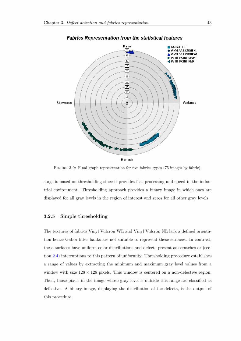
Chapter 3. Defect detection and fabrics representation 43
Figure 3.9: Final graph representation for five fabrics types (75 images by fabric).
stage is based on thresholding since it provides fast processing and speed in the indus-
trial environment. Thresholding approach provides a binary image in which ones are
displayed for all gray levels in the region of interest and zeros for all other gray levels.
3.2.5 Simple thresholding
The textures of fabrics Vinyl Vulcron WL and Vinyl Vulcron NL lack a defined orienta-
tion hence Gabor filter banks are not suitable to represent these surfaces. In contrast,
these surfaces have uniform color distributions and defects present as scratches or (sec-
tion 2.4) interruptions to this pattern of uniformity. Thresholding procedure establishes
a range of values by extracting the minimum and maximum gray level values from a
window with size 128 × 128 pixels. This window is centered on a non-defective region.
Then, those pixels in the image whose gray level is outside this range are classified as
defective. A binary image, displaying the distribution of the defects, is the output of
this procedure.

Chapter 4
RESULTS AND ANALYSIS
4.1 Description of the proposed system
A prototype is built to integrate the inspected fabric with the illumination sources, and
the camera. This structure provides an environment to test the proposed computer
vision based inspection system. Appendix B, presents the drawings of the proposed
system.
Figure 4.1 shows the flow diagram of the proposed system. First, the optical systems
is calibrated to estimate the intrinsic and extrinsic parameters. Then, user acquires a
fabric image that will be used to classify the fabric type and identify the type of defect.
4.2 Camera Calibration
4.2.1 Experimental set-up
Camera calibration is conducted on a experimental set-up with controlled illumination.
Appendix B presents the physical layout of the experimental set-up.
Fabrics samples will be placed on a uniform surface with dimensions 1.83 m by 1, 035 m.
This surface is located at a height of 0.93 m since a human operator will manipulate
the samples. Although camera diagonal field of view (FOV) covers 85% of surface area,
this coverage assures that the largest sample is included in the image acquired by the
44
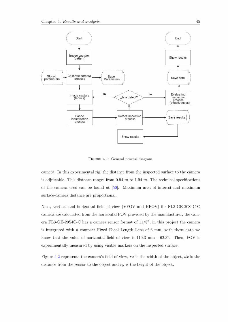
Chapter 4. Results and analysis 45
Figure 4.1: General process diagram.
camera. In this experimental rig, the distance from the inspected surface to the camera
is adjustable. This distance ranges from 0.94 m to 1.94 m. The technical specifications
of the camera used can be found at [50]. Maximum area of interest and maximum
surface-camera distance are proportional.
Next, vertical and horizontal field of view (VFOV and HFOV) for FL3-GE-20S4C-C
camera are calculated from the horizontal FOV provided by the manufacturer, the cam-
era FL3-GE-20S4C-C has a camera sensor format of 11/8”, in this project the camera
is integrated with a compact Fixed Focal Length Lens of 6 mm; with these data we
know that the value of horizontal field of view is 110.3 mm - 62.3◦. Then, FOV is
experimentally measured by using visible markers on the inspected surface.
Figure 4.2 represents the camera’s field of view, rx is the width of the object, dx is the
distance from the sensor to the object and ry is the height of the object.

Chapter 4. Results and analysis 46
dh
dx
rx
dy
ry
HFOV/2α
VF
OV
/2
Figure 4.2: Geometric projections - pinhole model.
Horizontal FOV - HFOV
HFOV = 2 ∗ arctan(tan(DFOV/2) ∗ cos(arctan(4/3)))
= 2 ∗ arctan(tan(73.2/2) ∗ cos(36.87)
= 61.3◦
HFOV and VFOV determines the total FOV at a given camera-object distance.
V FOV = 2 ∗ arctan(tan(DFOV/2) ∗ sin(arctan(3/4)))
= 2 ∗ arctan(tan(73.2/2) ∗ sin(36.87)
= 48◦
Next, the area of interest obtained with HFOV and VFOV specified by the manufacturer
is calculated.
Dmax = (1.93 m)− (0.93 m) = 1.0 m
dh = dx/(cos(DFOV/2))
dh = 1, 2456 m.
dy = dh ∗ (sin(DFOV/2))
dy = 0, 7426 m

Chapter 4. Results and analysis 47
With the data obtained we can calculate the angle:
θ = arctan(3/4)
θ = 36.87◦
Lateral sizes rx and ry determine the area of interest:
rx = dy ∗ cos θ
rx = 0, 7426 m ∗ cos 36.87◦
rx = 0, 594 m
ry = dy ∗ sinα
ry = 0, 7426 m ∗ sin 36.87◦
ry = 0, 445 m.
Hline = 2 ∗ rx
Hline = 1, 18 m.
Vline = 2 ∗ ry
Vline = 0, 89 m.
With the above calculations we can ensure that the height and width of the area of
interest for lighting are 1.18 m. and 0.89 m. These results state that the sides of the
total area of interest to be captured by the camera are 1.18 m and 0.89 m. However , this
design considers an additional 5% area to be illuminated. Figure 4.3 depicts this margin
and Figure 4.4 the table’s dimensions. We also consider a margin of 10% to capture the
images, i.e the possible capacity will subtract this safety margin to minimize distortion
effects in the borders, which ultimately leaves us with an ability to inspect parts with
dimensions of 1.062 m by 0.8 m. Figure 4.4 illustrates these sizes.
Now, the area of interest to be captured by the camera is measured in the experimental
configuration.

Chapter 4. Results and analysis 48
1,41157 m.
0,7
940 m
.0,8
337 m
.1,48214 m.
a
b
Figure 4.3: a) Area calculated by trigonometric projections - Pinhole model. b)Effective area with an additional margin of 5% for lighting.
Figure 4.4: Inspection areas.

Chapter 4. Results and analysis 49
Figure 4.5 illustrates the projection camera’s optical axis on the table surface, in this
image the vertical distance from the camera to the table is 1 m. Figure 4.6 illustrate
the markers placed on table surface.
Figure 4.5: Proposed prototype from a front view.
Figure 4.6: Markers on the table.
4.2.2 Results - comparison manual method
Tables 4.1 and 4.2 compare the experimental calculations of areas of interest against
those obtained from diagonal field of view (DFOV) data provided by camera manufac-
turer. A set of 10 length and width measurements supports this examination.
Table 4.1: Values obtained by geometry - pinhole model (meters).
Theoretical measuresWidth 1,18 m.Length 0,89 m.
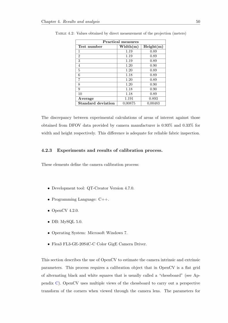
Chapter 4. Results and analysis 50
Table 4.2: Values obtained by direct measurement of the projection (meters)
Practical measuresTest number Width(m) Height(m)1 1.19 0.892 1.19 0.893 1.19 0.894 1.20 0.905 1.20 0.896 1.18 0.897 1.20 0.898 1.20 0.909 1.18 0.9010 1.18 0.89Average 1.191 0.893Standard deviation 0,00875 0,00483
The discrepancy between experimental calculations of areas of interest against those
obtained from DFOV data provided by camera manufacturer is 0.93% and 0.33% for
width and height respectively. This difference is adequate for reliable fabric inspection.
4.2.3 Experiments and results of calibration process.
These elements define the camera calibration process:
• Development tool: QT-Creator Version 4.7.0.
• Programming Language: C++.
• OpenCV 4.2.0.
• DB: MySQL 5.0.
• Operating System: Microsoft Windows 7.
• Flea3 FL3-GE-20S4C-C Color GigE Camera Driver.
This section describes the use of OpenCV to estimate the camera intrinsic and extrinsic
parameters. This process requires a calibration object that in OpenCV is a flat grid
of alternating black and white squares that is usually called a “chessboard” (see Ap-
pendix C). OpenCV uses multiple views of the chessboard to carry out a perspective
transform of the corners when viewed through the camera lens. The parameters for

Chapter 4. Results and analysis 51
this transform are contained in a 3 × 3 a homography matrix. The calibration pro-
cess acquires 20 views from the chessboard to obtain an error of 2%. Figure 4.7 shows
calibration pattern chessboard.
0
1 2 34
6 7 8
9 10 11 12 13 14
27 29 31 33 35
36 37 39 40 43
15 16
17 18 19 20 21 22 23 24 25
28 30 32 34
3841
42 44
45 46 47 48 49 50 51 52 53
Figure 4.7: Chessboard calibration pattern 5 x 4.
These steps describe the process followed to obtain the camera intrinsic and extrinsic
parameters:
1. Capture video streaming from the camera.
2. Capture and store chessboard distribution in still images.
3. Start camera calibration.
4. Estimate intrinsic and extrinsic parameters.
5. Presentation of results.
First, image resolution is set to 1600p x 1200p. Figure 4.8 shows the complete list of
parameters for image capture. Then, a streaming of video is acquired and the images of
the chessboard are captured and stored in a folder every 5 seconds. The program stores
the images in BMP format with a final size of 5.49 MB for each image.

Chapter 4. Results and analysis 52
Figure 4.8: Parameters for Calibration Process - (Flea3 FL3-GE-20S4C-C Color GigECamera).
To capture the parameter’s values of chess pattern, we implemented a simple interface
(see Appendix A).
4.2.3.1 Parameters of the function CalibrateCamera (OpenCV)
When calling a cvCalibrateCamera() several parameters must be defined such as:
ObjectPoints is an N × 3 matrix containing the physical coordinates of each of the K
points on each of the M images of the object. In a planar object like the chessboard we
can simply set all Z coordinates to zero.
ImagePoints is an N × 2 matrix containing the pixels coordinates of all the points
supplied in ObjectPoints.
ImageSize is the size of chessboard images extracted from the pixels.
CameraMatrix and distorsioncoeffs constitute the intrinsic parameters of the camera.

Chapter 4. Results and analysis 53
Previous two arguments summarize camera’s intrinsic information, the next two summa-
rize the extrinsic information. That is, they indicate the location of calibration objects
relative to the camera in each picture.
Rotationvectors is defined by a M three-component vectors arranged into an M − by−3
matrix where M is the number of images.
Translationvectors are similarly arranged into a second M × 3 matrix, again in the
camera coordinate system. The units of the camera coordinate system are exactly those
assumed for the chessboard.
flags argument allows finer control of exactly how the calibration will be performed.
4.2.3.2 Re-projection error estimation
The function CalibrateCamera returns the average re-projection error, which is the
results of averaging the errors of projecting image points into the object plane (i.e
chessboard) by using intrinsic and extrinsic parameters. Figure 4.9 shows the location of
chessboard pattern on the surface of the table during the calibration process. Figure 4.11
shows the calibration process results. Figure 4.10 shows the corners identified during
the calibration process.
Next, a validation procedure compares the dimensions provided by the computer vision
based system with respect to the sizes provided by a laser meter. Figure 4.12 shows the
circle and rectangle whose dimensions will be measured. The test follows these steps:
1. Generate video.
2. Capture image.
3. Prepocess the image with gaussian filtering.
4. Detect edges.
5. Measure the distance from the camera to the object through the intrinsic param-
eters estimated during the calibration process.

Chapter 4. Results and analysis 54
Figure 4.9: Sample images for the calibration process
Figure 4.10: Identification of corners during the calibration process
6. Compare results against manual measurements.
The first test consist of measuring the object-camera distance by using an object with
known dimensions. This reference object is a square with side L= 0,1 m. The reference
camera-object distance is 1 m. In these measurements, the relative error between the
mean value and the reference value is 0.46%. Table 4.3 presents mean and standard
deviation of measurement results after 10 evaluations.

Chapter 4. Results and analysis 55
Figure 4.11: Values of the parameters obtained in the calibration process
Figure 4.12: Shapes selecting for testing.
In the second test a circle diameter is measured given a known camera-object distance.
The reference circle diameter is 0.12 m. as shown in Figure 4.13, the discrepancy between
this reference value and the average of measured diameters as shown in table 4.4, is
0.03%.
Table 4.3: Measurement of the distance between the camera and the object (square).
Measurement Number Value(mm)1 991.9962 1007.4903 991.9964 992.0015 991.9966 996.6017 1001.8508 981.4969 979.80010 1018.640Average 995.387Standard deviation 11.606

Chapter 4. Results and analysis 56
Figure 4.13: Manual measurement of circle diameter D=120 mm.
Table 4.4: Measurement of circle diameter D=120 mm.
Measurement Number Value(mm)1 125.722 124.163 125.114 125.885 124.126 125.877 125.068 124.719 124.1910 124.80Average 124.962Standard deviation 0.6921

Chapter 4. Results and analysis 57
4.2.4 Evaluation of inspection methods
This section validates the proposed method to detect defects in fabrics with textures that
have either dominant directions or undefined orientations. This assessment is based on
ROC (Receiving operating characteristic) curves, which plot false positive rate against
true positive rate and account for the performance of the detection algorithm when
compared to human evaluations.
Previous works in this field such as [51] and [52] lack the information necessary to
understand the figures of merit deployed to evaluate the proposed methods. Figure 4.14
depicts a ROC curve.
Tru
e
Tru
e P
ositiv
e R
ate
50%
75%
100%
25% 50% 100%
False Positive Rate
Optimal point
Figure 4.14: ROC curve distribution.
The threshold in the ROC curve point with the highest true positive rate and lowest false
positive rate is of great interest to improve the performance of the proposed algorithm.
Hereafter, this point is named optimal point (OP).
A manual segmentation on the training data set provides the ground-truth to define the
figures of merit that measures the proposed methodology in this work, which are true
positive, false positive, and false negative. Figures 4.15a and 4.15b show a defective
fabric and the result of the manual segmentation.
ROC curves are calculated for each image extracting a AUC value from each ROC.
Therefore, AUC is the figure of merit to measure the performance of the segmentation
approaches proposed (Gabor filters and simple thresholding) on each image. 500 images

Chapter 4. Results and analysis 58
(a) Karyatide fabric defect. (b) Human (Manual) segmentation.
Figure 4.15: Kariatyde fabric defect and manual segmentation
(100 for each class) manually segmented images of fabrics with defects are the ground
truth.
4.2.5 Evaluation procedure
This section validates the proposed methodology based on ROC curves. These plots
represent the performance of the defect detection algorithm in the types of fabrics in-
spected. The area under ROC curve (AUC) summarizes in one scalar the performance
represented in each ROC curve. Figure 4.16 presents ROC curves for several images
obtained from fabric type petit point gray example, each curve corresponds to the eval-
uation of the method in a given image (4 images). In these curves each point expresses
a threshold. Appendix A shows the user interface screen to set this parameter in the
program. Figure 4.17 presents the results of the simple thresholding approach on 25 test
images. Figure 4.18 compares the defect detection provided by this approach with that
attained with manual segmentation. It is observed that AUC is greater than 0.9 in each
image and the results of automatic and manual segmentation are comparable.

Chapter 4. Results and analysis 59
0 0.2 0.4 0.6 0.8 10
0.1
0.2
0.3
0.4
0.5
0.6
0.7
0.8
0.9
1
FP Rate
TP
Rat
e
(a) ROC Curve for petit point gray fabricimage (D001).
0 0.2 0.4 0.6 0.8 10
0.1
0.2
0.3
0.4
0.5
0.6
0.7
0.8
0.9
1
FP Rate
TP
Rat
e
(b) ROC Curve for petit point gray fabricimage (D002).
0 0.2 0.4 0.6 0.8 10
0.1
0.2
0.3
0.4
0.5
0.6
0.7
0.8
0.9
1
FP Rate
TP
Rat
e
(c) ROC Curve for petit point gray fabricimage (D003).
0 0.2 0.4 0.6 0.8 10
0.1
0.2
0.3
0.4
0.5
0.6
0.7
0.8
0.9
1
FP Rate
TP
Rat
e
(d) ROC Curve for petit point gray fabricimages (D004).
Figure 4.16: ROC curves (individuals) for petit point gray fabric.
4.3 Parameter tuning for Gabor filter banks and simple
thresholding approach
In this work, Gabor filter banks and simple thresholding are means to segment fabric
images. Figures 4.19 and 4.20 present flow diagrams that describe these approaches. The
output of each procedure is a binary image indicating the presence of defects detected.

Chapter 4. Results and analysis 60
0 5 10 15 20 250
0.1
0.2
0.3
0.4
0.5
0.6
0.7
0.8
0.9
1
Defect Images
AU
C
Figure 4.17: AUC curve for images of fabric petit point red fabric (mean = 0.90876,standard deviation = 0.02488).
(a) Manual segmentation for Vinylvulcron W/L.
(b) Result of simple thresholding -Vinyl vulcron W/L.
Figure 4.18: Simple thresholding result and manual segmentation.
Even though the segmentation based on Gabor bank filters and simple thresholding
correlates well with human segmentation it is still necessary to tune parameters. For
instance, parameters such as scale and orientation in Gabor filter banks, and low and
high thresholds in simple thresholding have a wide range of possible values whose optimal
manual adjustment is difficult and cumbersome.
4.3.1 Gabor filters
Previous works estimate Gabor filter bank parameters based on the evaluation of the
highest contrast generated by convolving each filter with the same image as in [41].

Chapter 4. Results and analysis 61
Start Gaborfilter process
Select bestcombination
from bank filter
Apply Gabor
filter to defect
image
Presents Results
Mark a pixel
as defective
Is a pixel
out of theresolding
range/value?
Get central
window from
free-defect image
Compare defect
image filtered
vs
theresolding values
Presents blank
fields
for
parameters
Selection
image
path/folder
Fabric identification
End
Are theremore pixelsto evaluate?
Are thereparametersfor fabrics?
Figure 4.19: Diagram process - Gabor filters method
Figures 4.21, 4.22, 4.23 illustrate the results of convolving with an image of fabric Kary-
atide a bank of nine Gabor filters with a number of scales S=3 and orientations L=3.

Chapter 4. Results and analysis 62
Start simple
thresholding
Apply simple
thresholding
to defect image
Presents Results
Mark a pixel
as defective
A therere
more pixels
for evaluate?
Get central
window from
free-defect image
Compare defect
image filtered
vs
theresolding values
Presents blank
fields
for
parameters
A therere
parameters
for fabric?
Selection
image
path/folder
Fabric identification
End
Get thresholds
values
Yes
Is pixel (i,j)out of thresholding
range/value?
Figure 4.20: Diagram process - simple thresholding method

Chapter 4. Results and analysis 63
Figure 4.21: a)angle=0.00, frequency=0.125, α=2.449, σx=3.567, σy=0.433; b)angle=0.0, frequency=0.306, α=2.449, σx=1.456, σy=0.439; c) angle=0.0, fre-
quency=0.750, α=2.449, σx=0.594, σy=0.476
Figure 4.22: a)angle=1.0471, frequency=0.1250, α=2.449, σx=3.567, σy=0.433; b)angle=1.0471, frequency=0.306, α=2.449, σx=1.456, σy=0.439; c) angle=1.0471, fre-
quency=0.750, α=2.449, σx=0.594, σy=0.476
Figure 4.23: a)angle=2.0943, frequency=0.1250, α=2.449, σx=3.567, σy=0.433; b)angle=2.0943, frequency=0.306, α=2.449, σx=1.456, σy=0.439; c) angle=2.0943, fre-
quency=0.750, α=2.449, σx=0.594, σy=0.476
Gabor filter banks for defect detection in fabrics Karyatide, petit point gray, and petit
point red require the definition of a range of orientations to decide if a given pixel is
defective or non-defective. This work proposes a methodology based on genetic algo-
rithms to estimate the best set of parameters that maximizes the true positive rate of
the detection algorithm.

Chapter 4. Results and analysis 64
The variables in this process are high and low orientations, θh and θl, respectively. Fixed
values for the algorithm are kernel size, kernel angular steps and kernel frequency steps.
The main reason why we decided to fix values is that there is the prior knowledge of the
form in which the defects are manifested; primarily through lines on fabrics that have
a definite orientation. Parameter tuning is carried out on training data set, then, the
tuned parameters define a ROC curve, in which the threshold that provides the highest
true positive and the lowest false positive is selected to validate the procedure on the
test data set.
The objective function of the genetic algorithm is a threshold value φ of the average
AUC obtained from the training data set, AUC calculation is made using the trapezoid
rule.∫ b
af(x) dx ≈ 1
2
N∑
k=1
(xk+1 − xk) (f(xk+1) + f(xk)) (4.1)
The genetic algorithm starts with two parents, which means two values of θh, and two
values of θl. These are the inputs parameters:θh1, θh2, θl1, θl2
It is also necessary to compute the mutations and crossings which receive two additional
parameters that are mutation and crossover probabilities Pm and Pc.
The data set on which the genetic algorithm operates consists of 75 images for each type
of fabric. Each generation is performed by the application of the objective function on
35 randomly selected images for each pair of θh and θl values.
The genetic algorithm receives as parameters a population of two individuals, each
consisting of a value of θh and θl, and the probability of crossover Pc and mutation
probability Pc, these probabilities are validated at each generation of individuals.
To determine whether each iteration crosses or mutations are performed, a random
number between 0 and 1 is generated, if the generated value is less than Pc then a
crossover is performed, in the case of mutation is evaluated a new random number, if
this is less than Pm is executed to generate a new offspring.
Parents are converted to binary numbers to conduct the crossover and mutation oper-
ations, for mutation and crossing a random number between 1 and (l − 1) is chosen
(where l is the length of the string used to represent the individual, for crossing case the

Chapter 4. Results and analysis 65
obtained number indicates where parents are crossed, whereas for mutation the number
indicates the bit that must be mutated.
The objective function is the validation of defects with each generation of new individuals
obtained. If new individuals perform better than their parents, they become new parents
of the next generation, otherwise the cycle begins again with the previous parent. The
algorithm is executed while the evaluation result obtained parameter not exceeding the
value as a target. Figure 4.24 shows a diagram of the operation of the genetic algorithm.
4.3.2 Simple thresholding
Simple thresholding permits the segmentation of fabrics Vulcron vinyl WL and Vulcron
vinyl NL because their surfaces do not have defined orientations. The parameters for
this case are the lowest and highest gray level in a square window on a non-defective
region. To select the appropriate values of the thresholds these are changed manually
between 75% and 105% of their values, this is done in order to refine the values obtained
by thresholding process.

Chapter 4. Results and analysis 66
Figure 4.24: Diagram process - genetic algorithm.

Chapter 4. Results and analysis 67
4.4 Results
This section shows the results of parameter tuning and defect detection based on AUC
for each fabric type. In this validation, the training set is composed of images with the
prefix ”D” that range from D001 to D075 image. The training set is formed by the
set of images from D076 to D100. All images were taken with the camera described in
section 2.2 - Camera Calibration.
Table 4.5 describes the inspection process details, parameters, ROC curves, scales and
fabric images of technical details. For vulcron fabrics (vinyl W/L and vinyl N/L) the
images cover a smaller area of fabric, nevertheless; this decision is supported by the
lower computational cost of inspection method used.
D-min is the minimum value for plot ROC curves, D-max is the maximum value for plot
ROC curves and scale is the increment between D-min and D-max. Conversion factor
aids to balance the number of defective and non-defective pixels image by reducing their
sizes in the same proportion.
4.4.1 Analysis of results
Figures 4.26, 4.28, 4.30, 4.32 and 4.34 show the inspection process for training set, along
with defective and non-defective test sets. These results show that average AUC for the
test set is greater than 0.9.
4.4.1.1 Gabor filters method
For Gabor filters method, the parameter tuning with the proposed training data set
and genetic algorithm provides high AUC values and low false positive rates in images
without defects, simple thresholding results obtained with the non-defective test set are
satisfactory since they present low FP rates.
Kariatyde: evaluation of the parameters in the test set gives a true positive rate of 92%,
considering the size of the defect and its manifestation is a highly satisfactory result,
we must emphasize that the size of the images with which they worked are functionally

Chapter 4. Results and analysis 68
oriented to an automated system for detecting defects, meaning that these sizes are not
sacrificed to achieve the proposed goal.
Petit point gray: the results in terms of detection are the highest obtained with the
method of Gabor filters with 93.2% true positive rate, although the manifestation of the
defect in this fabric is visually more evident it should be noted that this can take any
shape or orientation by which the applicability of the method is demonstrated in these
conditions.
Petit point red:evaluation of the parameters in the test set gives a true positive rate of
90.9%, it is necessary to consider the fabric color is present on the surface which will
adds more complexity and computational cost image filtering.
For petit point red and petit point gray fabrics, OP reach very low values since the
defect is more evident in the inspection process without having to take high threshold
values, contrary to fabric karyatide where the defect is less noticeable so the process
takes higher OP values.
4.4.1.2 Simple thresholding
In Vulcron vinyl W/L and the Vulcron vinyl N/L fabric the detection level is reached to
90.2% and 90.3% respectively, in this case the results are essentially very similar because
the surface is the same in both fabrics. In the experiment we used different picture sizes
to analyze whether detection results improved by decreasing the object-camera distance,
but the improvement is only 0.01.

Chapter 4. Results and analysis 69
0 10 20 30 40 50 60 70 800.6
0.65
0.7
0.75
0.8
0.85
0.9
0.95
1
1 to 75 defect images(training set)
AU
C −
OP
− F
P r
ate
AUC−training set
OP−training set
Figure 4.25: Inspection process results - Kariatyde fabric (training set).
0 5 10 15 20 25 300.6
0.65
0.7
0.75
0.8
0.85
0.9
0.95
1
1 to 25 defect images(test set)
AU
C −
OP
− F
P r
ate
AUC−test set
Figure 4.26: Inspection process results - Kariatyde fabric (test set).

Chapter 4. Results and analysis 70
0 10 20 30 40 50 60 70 800.6
0.65
0.7
0.75
0.8
0.85
0.9
0.95
1
1 to 75 defect images(training set)
AU
C −
OP
− F
P r
ate
AUC−training set
OP−training set
Figure 4.27: Inspection process results - Vulcron vinyl W/L fabric (training set).
0 5 10 15 20 25 300.6
0.65
0.7
0.75
0.8
0.85
0.9
0.95
1
1 to 25 defect images(test set)
AU
C −
OP
− F
P r
ate
AUC−test set
Figure 4.28: Inspection process results - Vulcron vinyl W/L fabric (test set).

Chapter 4. Results and analysis 71
0 10 20 30 40 50 60 70 800.6
0.65
0.7
0.75
0.8
0.85
0.9
0.95
1
1 to 75 defect images(training set)
AU
C −
OP
− F
P r
ate
AUC−training set
OP−training set
Figure 4.29: Inspection process results - Vulcron vinyl N/L fabric (training set).
0 5 10 15 20 25 300.6
0.65
0.7
0.75
0.8
0.85
0.9
0.95
1
1 to 25 defect images(test set)
AU
C −
OP
− F
P r
ate
AUC−test set
Figure 4.30: Inspection process results - Vulcron vinyl N/L fabric (test set).

Chapter 4. Results and analysis 72
0 10 20 30 40 50 60 70 800.6
0.65
0.7
0.75
0.8
0.85
0.9
0.95
1
1 to 75 defect images(training set)
AU
C −
OP
− F
P r
ate
AUC−training set
OP−training set
Figure 4.31: Inspection process results - petit point gray fabric (training set).
0 5 10 15 20 25 300.6
0.65
0.7
0.75
0.8
0.85
0.9
0.95
1
1 to 25 defect images(test set)
AU
C −
OP
− F
P r
ate
AUC−test set
Figure 4.32: Inspection process results - petit point gray fabric (test set).

Chapter 4. Results and analysis 73
0 10 20 30 40 50 60 70 800.6
0.65
0.7
0.75
0.8
0.85
0.9
0.95
1
1 to 75 defect images(training set)
AU
C −
OP
− F
P r
ate
AUC−training set
OP−training set
Figure 4.33: Inspection process results - petit point red fabric (training set).
0 5 10 15 20 25 300.6
0.65
0.7
0.75
0.8
0.85
0.9
0.95
1
1 to 25 defect images(test set)
AU
C −
OP
− F
P r
ate
AUC−test set
Figure 4.34: Inspection process results - petit point red fabric (test set).

Chapter 4. Results and analysis 74
Table 4.5: Fabric images and inspection process details
Fabric Kariatyde
Inspection Method Gabor filters
Selected parameters θh = 0.967418; θl = 0.125984;
Selection method parameters Genetic algorithm
Average AUC obtained Training set 0.906; Test set 0.92
ROC-Curves D-min 0.01; D-max 1.21; scale 0.024
Conversion factor 0.3
Image size 1600 px × 1200 px
Fabric Vulcron vinyl W/L
Inspection Method Simple thresholding
Selected parameters factor = 0.966
Average AUC obtained Training set 0.9056; Test set 0.902
ROC-Curves D-min 0.8; D-max 1.0; scale 0.004
Conversion factor 0.16
Image size 1200 px × 1000 px
Fabric Vulcron vinyl N/L
Inspection Method simple thresholding
Selected parameters factor = 0.941
Average AUC obtained Training set 0.903; Test set 0.9036
ROC-Curves D-min 0.75; D-max 1.05; scale 0.006
Conversion factor 0.16
Image size 1000 px × 1000 px.
Fabric Petit point gray
Inspection Method Gabor filters
Selected parameters θh = 0.921; θl = 0.120;
Selection method parameters Genetic algorithm
Average AUC obtained Training set 0.915; Test set 0.932
ROC-Curves D-min 0.01; D-max 1.0; scale 0.04
Conversion factor 0.48
Image size 1600 px × 1200 px
Fabric Petit point red
Inspection Method Gabor filters
Selected parameters θh = 0.699; θl = 0.143;
Selection method parameters Genetic algorithm
Average AUC obtained Training set 0.907; Test set 0.909
ROC-Curves D-min 0.01; D-max 1.0; scale 0.03
Conversion factor 0.4
Image size 1400 px × 1000 px

Chapter 5
CONCLUSIONS AND FUTURE
WORK
5.1 Conclusions
Defect detection in fabrics with Gabor bank filters reach an average measured with AUC
equivalent to 0.92 for kariatyde, petit point red and petit point gray fabrics. Furthermore
defect detection in fabrics with simple thresholding reach a average measured with AUC
equivalent to 0.902 for vulcron vinyl W/L and vulcron vinyl N/L fabrics.
Although visual evaluations of fabrics conducted by human inspectors reaches a detection
rate of 87.5%, and the average performance of automatic assessment is 91%, it not
possible to carry out a fair comparison since the fabrics and illumination conditions
in the scenarios of human and automatic evaluations are different, given that optimal
conditions in which each method is performed, human as well as the developed system
are different, lighting conditions, distance vision and view angle developed by a human
are different to that of a machine vision system.
Gabor filters and simple thresholding methods are technically successful in terms of de-
fect detection performance as well as response times. Hence, both methods can support
an automated inspection system, considering the cost of the project and true positive
rates of the inspection system developed.
75

Chapter 5. Conclusions and future work 76
Genetic algorithms are useful methods to select Gabor filter banks parameters such as
orientations. This parameter selection aids to minimize FP rate in defect detection at
fabric digital images and contributes to increased levels of true positive rates. Inspected
all fabrics, the maximum rates of true positives was 99.3% whereas the minimum value
found in false positive is 0%.
Previous works [53], [8], [54], [55] have analyzed fabrics with different textures by using
Gabor filters. They report performances of 75%, 95%, 82.86% and 100%, respectively.
The results presented in this work present a performance of 92%. This performance is
close to those reported in previous works. However, unlike previous works this document
describes thoroughly the validation process and justifies the figures of merit such as AUC.
5.2 Future Work
Automation of computer vision based fabric inspection system by implanting mech-
anisms (i.e conveyor belt) that allow automatic movement of the fabric through the
system without human intervention.
Integrate the computer vision based fabric inspection software to the information system
of the production line.
Include additional types of defects and fabrics in the set of conditions detected by the
system.
Devise methods to inspect more defects and fabrics according to Table 2.6.
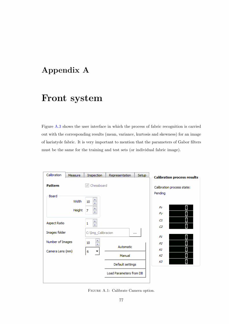
Appendix A
Front system
Figure A.3 shows the user interface in which the process of fabric recognition is carried
out with the corresponding results (mean, variance, kurtosis and skewness) for an image
of kariatyde fabric. It is very important to mention that the parameters of Gabor filters
must be the same for the training and test sets (or individual fabric image).
Figure A.1: Calibrate Camera option.
77

Appendix A. User interface 78
Figure A.2: Defect inspection option.

Appendix A. User interface 79
Figure A.3: Representation (Identification fabric type) option.

Appendix B
Prototype (C.E.)
80

Appendix
B.Prototype
81

Appendix C
Developer Guide
This work was performed under the Windows 7 operating system, but it was also tested
under Windows XP and Windows 8. For correct operation, the software needs the
following applications:
QT 4.7 Development Environment.
Flea3 FL3-GE-20S4C-C Color GigE Camera Driver.
OpenCv version 2.2.
ChartDirector version 5.0.3 to C++.
MySQL Server 5.1 or higher.
The OpenCv library is already compiled, so only need to copy the folder C OpenCV2.2MinGW,
ChartDirector folder must unzip and place on C:
Installation sequence:
1. QT Development Environment and RDBMS MySQL.
2. Copy qsqlmysqld4.dll library from MySQL folder to sqldrivers folder of QT installa-
tion, i.e. C:\Qt\2014 \qt\plugins\sqldrivers.3. Create a Empty DB and import data.
4. Open project with QT.
82

Appendix C. Developer Guide 83
tbl_auc
Indexes
Constraints
set_int_id M
fab_int_id D
auc_str_filename V
auc_num_inflexion D
tbl_defect
Constraints
fab_int_id DE…
def_int_id DE…
def_str_name VA…
def_str_description VA…
def_str_state VA…
tbl_setup
Constraints
set_int_id M…
set_num_dmin D…
set_num_dmax D…
set_num_escala D…
tbl_fabric
Constraints
fab_int_id DE
fab_str_name VA
fab_str_description VA
fab_str_state VA
tbl_measure
Indexes
Constraints
fab_int_id D…
set_int_id M…
mea_str_filename V…
mea_num_escala D…
tbl_par…
tbl_settings
Constraints
fab_int_id D
stg_chr_estado V
stg_int_id D
stg_chr_rem_blanco V
stg_chr_rem_negro V
stg_int_mask_conv D
stg_int_mask_kernel D
stg_num_ang_fh D
stg_num_ang_fl D
stg_num_dmin D
stg_num_dmax D
stg_num_escala D
stg_fecha D
stg_aplica_lim_inf V
stg_aplica_lim_sup V
stg_aplica_media V
stg_aplica_gauss V
stg_aplica_ecual V
tbl_stats
Constraints
fab_int_id D…
sta_filename V…
tbl_user
Indexes
Constraints
codigo INT
FK_tbl_auc_tbl_fabric
FK_tbl_auc_tbl_setup
FK_defect
FK_tbl_measure
FK_tbl_measure_fab
FK_tbl_settings_tbl_fabric
FK_tbl_stats
Figure C.1: Entity-relation model.

Appendix
C.Develo
perGuide
84
Figure C.2: Chessboard pattern - 9x7 squares.

Appendix D
User guide
This section describes the use cases for the processes of calibration, representation, and
defect inspection.
A use case is a complete list of steps, typically defining interactions between an actor
and a system, to achieve a goal. The actor can be a human, or an external system.
In this document two actors are identified, these are the operator and the system ad-
ministrator.
85
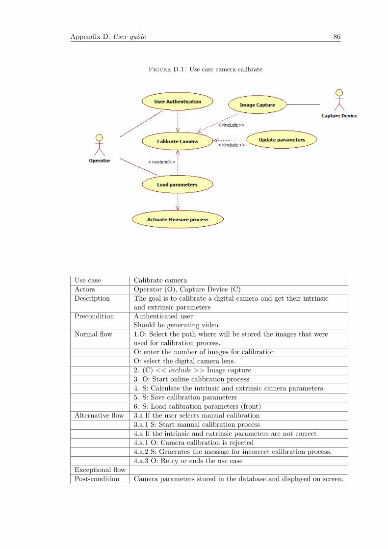
Appendix D. User guide 86
Figure D.1: Use case camera calibrate
Use case Calibrate camera
Actors Operator (O), Capture Device (C)
Description The goal is to calibrate a digital camera and get their intrinsicand extrinsic parameters
Precondition Authenticated userShould be generating video.
Normal flow 1.O: Select the path where will be stored the images that wereused for calibration process.
O: enter the number of images for calibration
O: select the digital camera lens.
2. (C) << include >> Image capture
3. O: Start online calibration process
4. S: Calculate the intrinsic and extrinsic camera parameters.
5. S: Save calibration parameters
6. S: Load calibration parameters (front)
Alternative flow 3.a If the user selects manual calibration
3.a.1 S: Start manual calibration process
4.a If the intrinsic and extrinsic parameters are not correct
4.a.1 O: Camera calibration is rejected
4.a.2 S: Generates the message for incorrect calibration process.
4.a.3 O: Retry or ends the use case
Exceptional flow
Post-condition Camera parameters stored in the database and displayed on screen.

Appendix D. User guide 87
Figure D.2: Use case fabric representation
Use case Representation fabric
Actors Operator (O), Capture Device (C)
Description The goal is to identify a fabric from the extraction offeatures of an image and compared against data previouslyobtained from a training set.
Precondition Data obtained from the representation (training set) of all fabrics.Authenticated user
Normal flow 1. << include >> Image capture
2. S: Load Gabor filter parameters
3. O: Start individual Identification process
3. S: Feature extraction of fabric image
4. S. Compare obtained features of the current image againstthe data training set
5. S: Presenting results
6. S: Save results
Alternative flow 1. O: Select the path where will be stored the images that wereused for identification (representation) process.
1.a S: Start manual calibration process
2. O: If the parameters do not exist
2.a O: Enter/Update Gabor filter parameters
Exceptional flow
Post-condition Fabric image identified, results stored
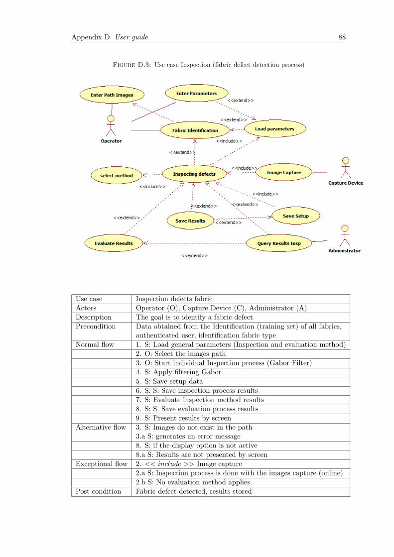
Appendix D. User guide 88
Figure D.3: Use case Inspection (fabric defect detection process)
Use case Inspection defects fabric
Actors Operator (O), Capture Device (C), Administrator (A)
Description The goal is to identify a fabric defect
Precondition Data obtained from the Identification (training set) of all fabrics,authenticated user, identification fabric type
Normal flow 1. S: Load general parameters (Inspection and evaluation method)
2. O: Select the images path
3. O: Start individual Inspection process (Gabor Filter)
4. S: Apply filtering Gabor
5. S: Save setup data
6. S: S. Save inspection process results
7. S: Evaluate inspection method results
8. S: S. Save evaluation process results
9. S: Present results by screen
Alternative flow 3. S: Images do not exist in the path3.a S: generates an error message
8. S: if the display option is not active
8.a S: Results are not presented by screen
Exceptional flow 2. << include >> Image capture
2.a S: Inspection process is done with the images capture (online)
2.b S: No evaluation method applies.
Post-condition Fabric defect detected, results stored

Appendix D. User guide 89
Figure D.4: Use case Inspection (fabric defect detection process)
Use case Inspection defects fabric
Actors Operator (O), Capture Device (C), Administrator (A)
Description The goal is to identify a fabric defect
Precondition Data obtained from the Identification (training set) of all fabrics,authenticated user, identification fabric type
Normal flow 1. S: Load general parameters (Inspection and evaluation method)
2. O: Select the images path
3. O: Start individual Inspection process (simple theresolding)
4. S: Apply filtering simple theresolding
5. S: Save setup data
6. S: S. Save inspection process results
7. S: Evaluate inspection method results
8. S: S. Save evaluation process results
9. S: Present results by screen
Alternative flow 3. S: Images do not exist in the path3.a S: generates an error message
8. S: if the display option is not active
8.a S: Results are not presented by screen
Exceptional flow 2. << include >> Image capture
2.a S: Inspection process is done with the images capture (online)
2.b S: No evaluation method applies.
Post-condition Fabric defect detected, results stored

Bibliography
[1] A. Aponte. Aplicacion de tecnicas de vision artificial para la inspeccion visual de
recubrimiento de cable. Master’s thesis, Pontificia Universidad Javeriana, Colombia,
2012.
[2] Gary Bradski and Adrian Kaehler. Learning OpenCV computer vision with the
OpenCV Library. O’Reilly, USA, first edition, 2008. ISBN 978-0-596-51613-0.
[3] OIT. Enciclopedia de salud y seguridad en el trabajo, July 2014. URL
http://www.ilo.org/global/topics/safety-and-health-at-work/WCMS_
162039/lang--es/index.htm.
[4] Industrias Notecaucanas S.A.S. Inorca s.a.s., February 2015. URL http://www.
inorca.com.
[5] Ankit Chaudharyc Jagdish L. Rahejaa, Bandla Ajayb. Real time fabric defect
detection system on an embedded dsp platform. Optik, Article in press, 2013.
[6] P. Mitropoulos Y.A. Karayiannis, R. Stojanovic. Defect detection and classifica-
tion on web tex-tile fabric using multiresolution decomposition and neural networks.
Proceedings of 6th IEEE International Conference on Electronics, Circuits andSys-
tems, pages 765–768, 5-8 September 2009.
[7] C.H. Chan and G.K.H. Pang. Fabric defect detection by fourier analysis. IEEE
Trans. Industry Applications, 36:1267–1276, October 2000.
[8] Ankit Chaudharyc Jagdish Lal Rahejaa, Sunil Kumarb. Fabric defect detection
based on glcm and gabor filter: A comparison. Optik, Article in Press:0–1, 2013.
[9] H. Golnabi and A. Asadpour. Design and application of industrial machine vision
systems. Robotics and Computer-Integrated Manufacturing, 23:630–637, 2007.
90

Bibliography 91
[10] D. Sannen and H. Van Brussel. A multilevel information fusion approach for visual
quality inspection. Information Fusion, 13:48–59, 2012.
[11] P. Facco and A.Masiero. Improved multivariate image analysis for product quality
monitoring. Chemometrics and Intelligent Laboratory Systems, 109:42–50, 2011.
[12] H.K. Mebatsion and J. Paliwal. Machine vision based automatic separation of
touching convex shaped objects. Computers in Industry, 63(1):723–730, 2012.
[13] J. Denzler E. S. Wacker. Enhanced anomaly detection in wire ropes by combining
structure and appearance. Pattern Recognition Letters, 34:942–953, 2013.
[14] H. Eldeeb A. Abouelela, H. Abbas. Automated vision system for localizing struc-
tural defects in textile fabrics. Pattern Recognition Letters, 26:1435–1443, 2005.
[15] Elbit Vision Systems. I-tex system, February 2015. URL http://www.evs.co.il.
[16] BarcoVision’s. Cyclops, February 2015. URL http://www.visionbms.com/
textiles.
[17] Zellweger Uster’s. Fabriscan, February 2015. URL http://www.uster.com.
[18] K.F.C. Yiu K.L. Mak, P. Peng. Fabric defect detection using morphological filters.
Image and Vision Computing, 27:1585–1592, 2009.
[19] S. Serikawa S. Hossain. Texture databases – a comprehensive survey. Pattern
Recognition Letters, Article in Press, 2013.
[20] Patil P.M. Mahajan P.M, Kolhe S.R. A review of automatic fabric defect detection
techniques. Advances in Computational Research, 1:18–29, 2009.
[21] R. Ebrahimpour M. Tabassian, R. Ghaderi. Knitted fabric defect classification for
uncertain labels based on dempster–shafer theory of evidence. Expert Systems with
Applications, 38:5259–5269, 2011.
[22] A. Latif-Amet and A. Ertutzun. An efficient method for texture defect detection:
sub-band domain co-occurrence matrices. Image and Vision Computing, 18:543–
553, 2000.
[23] Nelson H.C. Yung Henry Y.T. Ngan, Grantham K.H. Pang. Automated fabric
defect detection—a review. Image and Vision Computing, 29:442–458, 2011.

Bibliography 92
[24] X. Yang H. Zuo, Y. Wang. A timely detection of a coated board streak defect in sub-
sampling conditions using monochrome vision system. 5th International Congress
on Image and Signal Processing, 2012.
[25] C. Duchesne and J.J. Liu. Multivariate image analysis in the process industries: A
review. Chemometrics and Intelligent Laboratory Systems, 117:116–128, 2012.
[26] L. Bissi and G. Baruffa. Automated defect detection in uniform and structured
fabrics using gabor filters and pca. J. Vis. Commun. Image R., 24:838–845, 2013.
[27] E.S. Gadelmawla. Computer vision algorithms for measurement and inspection of
spur gears. Measurement, 44:1669–1678, 2011.
[28] Henry Y. T. Ngan and Grantham K. H. Pang. Regularity analysis for patterned
texture inspection. IEEE Transactions on Automation Science and Engineering, 6:
131–144, January 2009.
[29] J. Zhou and J. Wang. Fabric defect detection using adaptive dictionaries. Textile
Research Journal, 83:1846–1859, 2013.
[30] Xiu-bao Huang Hong-gang Bu, Jun Wang. Fabric defect detection based on multiple
fractal features and support vector data description. Engineering Applications of
Artificial Intelligence, 22:224–235, September 2009.
[31] Du-Ming Tsai and Tse-Yun Huang. Automated surface inspection for statistical
textures. Image and Vision Computing, 21:307–323, 2003.
[32] Z. X. Liu and W. Zhixun Su. Slub extraction in woven fabric images using gabor
filters. Textile Research Journal, 78:320–325, 2008.
[33] K.L. Mak and P. Peng. An automated inspection system for textile fabrics based on
gabor filters. Robotics and Computer-Integrated Manufacturing, 24:359–369, 2013.
[34] Grantham K. H. Pang Ajay Kumar. Defect detection in textured materials using
gabor filters. IEEE Transactions on Industry Appkications, 38:425–438, 4 2002.
[35] N. Yung X. Yang, G. Pang. Discriminative training approaches to fabric defect
classification based on wavelet transform. Pattern Recognition, 37:889–899, 2004.
[36] S.P.Yung Henry Y.T. Ngan, Grantham K.H. Pang. Wavelet based methods on
patterned fabric defect detection. Pattern Recognition, 38:559–576, 2005.

Bibliography 93
[37] W.K. Won and C.W. Yuen. Stitching defect detection and classification using
wavelet transform and bp neural network. Expert Systems Application, 36:3845–
3856, 2009.
[38] Inter Corporation. Oficial documentation. OpenCV, 2014.
[39] Point Grey. Flea R©3 (gige vision), July 2014. URL http://www.ptgrey.com/
products/flea3_gige/flea3_gige_camera.asp.
[40] Osaky Colombia. Web, June 2014. URL http://www.osaky.net/test/index.asp.
[41] D. Gabor. Theory of communication, 09 1945.
[42] John G. Daugman. Uncertainty relation for resolution in space, spatial, frequency
and orientation optimized by two-dimensional visual cortical filters. J. Opt. Soc.
Am, 2:1160–1168, 7 1985.
[43] B.S. Manjunathi and W.Y. Ma. Texture features for browsing and retrieval of
image data. IEEE Transactions in Pattern Analysis and machine Intelligence, 18:
837–842, 8 1996.
[44] Hak Wee Tang; Venugopal Srinivasan; Sim Heng Ong. Texture features for browsing
and retrieval of image data. Optical Engineering, 34:125–134, 1 1995.
[45] Yuan Ye. Fabric defect detection using fuzzy inductive reasoning based on im-
age histogram statistic variables. In 2009 Sixth International Conference on Fuzzy
Systems and Knowledge Discovery, pages 191–194, Beijing, China, 2009.
[46] Min Dong Hui Yu Jiang and Wei Li. Detection of fabric defect based on optimal
tree structure of wavelet decomposition. In International Symposium on Intelligent
Ubiquitous Computing and Education, pages 210–213, Wuhan, China, 2009.
[47] J. Zhang and G. Baciu. Idss: A novel representation for woven fabrics. IEEE
Transactions on visualization and computer graphics, 19(3):122–131, March 2003.
[48] Aapo Hyvarinen. Independent Component Analysis. Wiley, USA, first edition, 2001.
ISBN 0-471-40540-X.
[49] P. Mahalanobis. On the generalized distance in statistics. In Proceedings of the
National Institute of Science 12, pages 49–55, USA, 1936.

Bibliography 94
[50] Point Grey. Gige digital camera - imaging performance specification, June
2014. URL www.ptgrey.com/support/downloads/downloads_admin/dlhelper.
aspx?vp=FL3-GE_ImagingPerformance.pdf&dld=230.
[51] Xin Liu and Imam Samil Yetik. A new roc analysis method considering the corre-
lation between neighboring pixels. In 34th Annual International Conference of the
IEEE EMBS, pages 4422–4425, San Diego, California USA, 2012.
[52] Cao Li Wang Xu-hui, Shu Ping and Wang Ye. A roc curve method for performance
evaluation of support vector machine with optimization strategy. In 2009 Inter-
national Forum on Computer Science-Technology and Applications, pages 117–120,
Beijing, China, 2009.
[53] H. Nishikado N. Ogata, S. Fukuma and A. Shirosakii. An accurate inspection of pdp-
mesh cloth using gabor filter. Proc. IEEE Int’l Sym. Intelligent Signal Processing
and Communication Systems, pages 65–68, 2005.
[54] S. Latham A. Bodnarova, M. Bennamoun. Optimal gabor filter for textile flaw
detection. Pattern Recognition, 35(35):2973–2991, 2002.
[55] M.S. Millan J. Escofet, R. Navarro and J. Pladellorens. Optimal gabor filter for
textile flaw detection. Optical Engineering, 35(37):2297–2307, 8 1998.