Detection of Prostate Cancer from Whole-Mount Histology ImagesUsing Markov Random Fields

James P. Monaco1, John E. Tomaszewski2, Michael D. Feldman2, Mehdi Moradi3, Parvin Mousavi3, AlexanderBoag4, Chris Davidson4, Purang Abolmaesumi3, Anant Madabhushi1

1Department of Biomedical Engineering, Rutgers University,USA.2Department of Surgical Pathology, University of Pennsylvania, USA.

3School of Computing, Queen’s University, Canada.4Department of Pathology, Queen’s University, Canada.

Abstract— Annually in the US 186, 000 men are diagnosed withprostate cancer (CaP) and over43, 000 die from it. The analysisof whole-mount histological sections (WMHSs) is needed to helpdetermine treatment following prostatectomy and to create the“ground truths” of CaP spatial extent required to evaluateother diagnostic modalities (eg. magnetic resonance imaging).Computer aided diagnosis (CAD) of WMHSs could increaseanalysis throughput and offer a means for identifying imagebased biomarkers capable of distinguishing, for example, CaPprogressors from non-progressors. In this paper we introduceaCAD algorithm for detecting CaP in low-resolution WMHSs. Atlow-resolution the prominent visible structures are glands. Sincecancerous and benign glands differ in size, gland area providesa discriminative feature. Additionally, cancerous glands tend tobe near other cancerous glands. This information is modeledusing Markov random fields (MRFs). However, unlike most MRFstrategies which rely on heuristic formulations, we introduce anovel methodology that allows the MRF to be modeled directlyfrom training data. Our CAD system identifies cancerous regionswith a sensitivity of 0.8670 and a specificity of0.9524.

I. I NTRODUCTION

Annually in the US186, 000 people are diagnosed withprostate cancer (CaP) and over43, 000 die from it. Theexamination of histological specimens remains the definitivetest for diagnosing CaP. Though the majority of such analysisis performed on core biopsies, the consideration of whole-mount histological sections (WMHSs) is also important. Fol-lowing prostatectomy, the staging and grading of WMHSs helpdetermine prognosis and treatment. Additionally, the spatialextent of CaP as established by the analysis of WMHSscan be registered to other modalities (eg. magnetic resonanceimaging), providing a “ground truth” for evaluation. Thedevelopment of computer aided diagnosis (CAD) algorithmsfor WMHSs is also significant: 1) CAD offers a viable meansfor analyzing the vast amount of the data present in WMHSs,a time-consuming task currently performed by pathologists,2) the consistent, quantified features and results inherenttoCAD systems can be used to refine our own understanding

This work was made possible due to grants from the Wallace H. Coulterfoundation, New Jersey Commission on Cancer Research, the National CancerInstitute (R21CA127186-01, R03CA128081-01), the Societyfor Imaging andInformatics on Medicine, and the Life Science Commercialization Award.

Corresponding authors: James Monaco, email: jpmonaco@rci.rutgers.edu,Anant Madabhushi email: anantm@rci.rutgers.edu

of prostate histology, thereby helping doctors improve perfor-mance and reduce variability in grading and detection, and3) the data mining of quantified morphometric features mayprovide means for biomarker discovery, enabling for example,the discrimination of CaP progressors from non-progressors.

With respect to prostate histology Begelman [1] considerednuclei segmentation for hematoxylin and eosin (H&E) stainedprostate tissue samples. In [2] Naik used features derived fromthe segmentation of nuclei and glands to determine Gleasongrade in core biopsy samples. To aid in manual cancer diag-nosis Gao [3] applied histogram thresholding to enhance theappearance of cytoplasm and nuclei. In this paper we introducethe first CAD system for detecting CaP in WMHSs. Thissystem is specifically designed to operate at low-resolution(0.01mm2 per pixel) and will eventually constitute the initialstage of a hierarchical analysis algorithm, identifying areasfor which a higher-resolution examination is necessary. Assubstantiated in our previous approach [4] for prostate biopsyspecimens, a hierarchical methodology provides an effectivemeans for dealing with high density data (prostate WMHSshave 500 times the amount of data compared to a fourview mammogram). Even at low resolutions, gland size andmorphology are noticeably different in cancerous and benignregions [5]. In fact, we will demonstrate that gland size aloneis a sufficient feature for yielding an accurate and efficientalgorithm. Additionally, we leverage the fact that cancerousglands tend to be proximate to other cancerous glands. Thisinformation is modeled using Markov random fields (MRFs).However, unlike the preponderance of MRF strategies (suchas the Potts model) which rely on heuristic formulations, weintroduce a novel methodology that allows the MRF to bemodeled directly from training data.

Our CAD algorithm proceeds as follows: 1) gland segmen-tation is performed on the luminance channel of a color H&Estained WMHS, producing gland boundaries, 2) the systemthen calculates morphological features for each gland, 3) thefeatures are classified, labeling the glands as either malignantor benign, 4) the labels serve as the starting point for theMRF iteration which then produces the final labeling, and 5)the cancerous glands are consolidated into regions. Section IIconsiders these steps in detail. In Section III we discuss theresults of applying our algorithm to WMHSs. In Section IVwe present our concluding remarks.

Fig. 1. Example of current segmented region (CR), internal boundary (IB),and current boundary (CB) during a step of the region growingalgorithm.

II. M ETHODOLOGY

A. Gland Segmentation

In the luminance channel of histological images glandsappear as regions of contiguous, high intensity pixels circum-scribed by sharp, pronounced boundaries. To segment theseregions we adopt a routine first used for segmenting breastmicrocalcifications [6]. We briefly outline this algorithm.Firstdefine the following: 1)current region(CR) is the set of pixelsrepresenting the segmented region in the current step of thealgorithm, 2)current boundary(CB) is the set of pixels thatneighbor CR in an 8-connected sense, but are not in CR, and3) internal boundary(IB) is the subset of pixels in CR thatneighbor CB. These definitions are illustrated in Figure 1. Thegrowing procedure begins by initializing CR to a seed pixelassumed to lie within the gland. At each iteration CR expandsby aggregating the pixel in CB with the greatest intensity. CRand CB are updated, and the process continues. The algorithmterminates when theL∞ norm from the seed to the nextaggregated pixel exceeds a predetermined threshold. That is,the L∞ norm establishes a square bounding box about theseed; the growing procedure terminates when the algorithmattempts to add a pixel outside this box. During each iterationthe algorithm measures the boundary strength which is definedas the average intensity of the pixels in IB minus the averageintensity of the pixels in CB. After the growing procedureterminates, the region with the greatest boundary strengthis selected. Seed pixels are established by finding peaks inthe image after Gaussian smoothing. Since gland sizes canvary greatly, we smooth at multiple scales, each of whichis defined by the sigmaσg ∈ {0.2, 0.1, 0.05, 0.025}mm ofa Gaussian kernel.1 The lengthl of each side of the boundingbox used for terminating the segmentation step is tied to thescale: l = 12σg. The final segmented regions may overlap.In this event the region with the highest boundary measureis retained. Figures 2(a) and 2(g) are H&E stained WMHSswith black ink marks providing a rough truth (RT) of CaPextent. Gland segmentation results are shown in Figures 2(b)and 2(h). Figures 2(c) and 2(i) provide magnified views ofthe regions of interest in Figures 2(b) and 2(h). The centroidsof glands whose probability of malignancy exceedsρ = 0.15are marked with green dots in Figures 2(d) and 2(j)2. Thislabeling is refined by the MRF iteration, producing the gland

1The growing procedure operates on the original image.2Figures 2(d), 2(j), 2(e), 2(k), 2(f) and 2(l) will be furtherexplained in later

sections.

centroids shown in Figures 2(e) and 2(k). Figures 2(f) and 2(l)show the aggregation of cancerous glands into regions (green)along with a high-fidelity truth (HFT) of CaP extent (yellow).

B. Feature Extraction, Modeling, and Bayesian Classification

Gland area is used to discriminate benign from malignantglands. Since we employ a Bayesian framework, we require es-timates of the conditional probability density functions (pdfs)of gland area for both malignantωm and benignωb glands.Using the equivalent square root of gland area (SRGA), thepdfs f

(

y∣

∣ωm

)

andf(

y∣

∣ωb

)

can be accurately modeled witha weighted sum of gamma distributions:

f (y; θ, k, λ) = λyk1−1e−y/θ1

θk1

1Γ (k1)

+ (1−λ) yk2−1e−y/θ2

θk2

2Γ (k2)

,

(1)wherey > 0 is the SRGA,λ∈ [0, 1] is the mixing parameter,k1, k2 > 0 are the shape parameters,θ1, θ2 > 0 are the scaleparameters, andΓ is the Gamma function. Note, we usef toindicate a continuous pdf andp to denote a discrete probabilitymass function (pmf). A Bayesian classifier uses these pdfs tocalculate the probability of malignancy for each gland. Thoseglands whose probabilities exceed the predetermined thresholdρ are labeled malignant; the remainder are classified as benign(Figures 2(d) and 2(j)).

C. Improved Classification Using Markov Random Fields

In addition to glandular features such as area, a highlyindicative trait of cancerous glands is their proximity to othercancerous glands. This can be modeled using MRFs.

1) Formulation of Gland Proximity as a MRF:Let S ={s1, s2, . . . , sN} represent a set ofN unique sites correspond-ing to the N segmented glands. Let each sites ∈ S havean associated random variableXs ∈ {ωm, ωb} indicating itsstate as either malignant or benign. To refer collectively tothe states of all glands we haveX = {Xs : s∈S}. Eachstate Xs is unknown; we only observe an instance of therandom variableYs ∈ R

D representing theD dimensionalfeature vector associated with glands. Though our algorithmis extensible to any number of features, currentlyD=1 withYs being the SRGA. To collectively refer to the entire sceneof feature vectors we haveY ={Ys : s∈S}.

Fig. 3. Graph with six sites and binary states.

Consider the undirected graphG = {S,E}, where the setS of sites represents the vertices and the setE contains the

(a) (b) (c)

(d) (e) (f)

(g) (h) (i)

(j) (k) (l)

Fig. 2. (a), (g) H&E stained prostate histology sections withblack ink mark indicating RT. (b), (h) Gland segmentation boundaries. (c), (i) Magnified viewsof white boxes from (b), (h). Centroids of cancerous glands before (d), (j) and after (e), (k) MRF iterations. (f), (l) Estimated cancerous regions (green) withHFT (yellow).

edges. A local neighborhoodηs is defined as follows:ηs ={r : r∈S, r 6= s, {r, s}∈E}. The set of all local neighbor-hoods establishes a neighborhood structure:η = {ηs : s ∈ S}.A clique is a set of the vertices of any fully connected subgraphof G. The setC contains all possible cliques. These conceptsare best understood in the context of an example. The graph

in Figure 3 has sitesS = {1, 2, 3, 4, 5, 6} and edgesE ={{1, 2} , {1, 4} , {1, 5} , {2, 3} , {2, 6} , {4, 5}}. The neighbor-hood of site5, for example, isη5 = {1, 4}. There are sixone-element cliquesC1 = {{1} , {2} , {3} , {4} , {5} , {6}},six two-element cliquesC2 =E, and one three-element cliqueC3 = {{1, 4, 5}}. The set C is the union of these three

sets. The stateXs of each site is either black or white, i.e.Λ={b,w}. Our specific neighborhood structure is determinedby the distance between gland centroids. Ifms denotes thecentroid of glands, thenr ∈ ηs if ‖ms−mr‖2

<d. Motivatedby the pathology we choosed=0.7mm.

To simplify notation we usePr {Xr = xr,Xs = xs} ≡p (xr, xs) for indicating the probability of a specific event,wherexr, xs ∈{ωm, ωb}. If X is a MRF with respect to theneighborhood structureη, then X satisfies the local Markovproperty p

(

xs

∣

∣x-s)

= p(

xs

∣

∣xηs

)

, where x-s indicates x

without xs andxηs={xs : s ∈ ηs}. Additionally, X is a MRF

with respect toη if and only if p (x) is a Gibbs distribution[7]: p (x)=

∏

c∈CVc (x), whereVc are nonzero functions that

depend only on thosexs for which s∈c. The local conditionalprobabilities follow directly:

p(

xs

∣

∣xηs

)

=p(xs, xηs

)∑

ω∈Λp(ω, xηs

)=

p(x)∑

ω∈Λp(ω, x-s)

=

∏

c:s/∈cVc(x)∏

c:s∈cVc(x)∏

c:s/∈cVc(x)∑

ω∈Λ

∏

c:s∈cVc(ω, x-s)

=

∏

c:s∈cVc(x)∑

ω∈Λ

∏

c:s∈cVc(ω, x-s). (2)

This distribution has the same form as the Gibbs distributionfor p (x), but now the product is only over those cliquesc thatcontains.

2) Integration of Data Derived PMFs into the MRF:Sinceit is difficult to derive Gibbs distributions that model a setoftraining data, generic models are usually assumed. The mostprevalent formulation is the Potts model which is defined asfollows for two-element cliques:

V{r,s} (xr, xs) =

{

e−β if xr = xs and {r, s} ∈ C

eβ if xr 6= xs and {r, s} ∈ C.(3)

The Potts model disregards all cliques having more or lessthan two elements, i.e. if|c| 6= 2 we haveVc (x) = 1, where|·| signifies cardinality. Such generic models are unnecessary;assuming that allXs are i.i.d. and allXr givenXs are i.i.d. foreveryr∈ηs, we can determine the appropriateVc directly fromthe data. To our knowledge, the following equations representthe first proposed means for incorporating arbitrary pmfs intothe MRF structure:

Vs (xs) = p (xs)1−|ηs| for s ∈ S (4)

V{r,s} (x) = p (xr, xs) for {r, s} ∈ C. (5)

The functionsVc for higher-order cliques are identically one.The validity of (4) and (5) can be seen by inserting them into(2):

∏

c:s∈cVc(x)∑

ω∈Λ

∏

c:s∈cVc(ω, x-s)=

p (xs)1−|ηs| ∏

r∈ηs

p (xr, xs)∑

ω∈Λp (ω)

1−|ηs| ∏

r∈ηs

p (xr, ω)

=p (xs)

∏

r∈ηs

p(

xr

∣

∣xs

)

∑

ω∈Λp (ω)

∏

r∈ηs

p(

xr

∣

∣ω)

=p (xs, xηs

)∑

ω∈Λp (ω, xηs

)=p

(

xs

∣

∣xηs

)

.

The determination ofp (xs) and p (xr, xs) from trainingdata is straight-forward. For example, consider the randomly

selected two-element clique{r, s} where both sites are ma-lignant. The probabilityV{r,s} (ωm, ωm) = p (ωm, ωm) canbe found by examining all permutations of two neighboringglands and determining the percentage in which both arecancerous. The pmfp (xs) is the marginal mass function ofp (xr, xs). Sincep (xr, xs) is symmetric, both marginals areidentical.

3) Label Estimation and Aggregation:The goal is to es-timate the hidden statesX given the observationsY usingmaximum a posteriori (MAP) estimation, i.e. maximizingp

(

x∣

∣y)

over x. Bayes laws yieldsp (x|y) ∝ f (y|x) p (x),where ∝ signifies proportionality. The Iterated ConditionalModes (ICM) [8] algorithm indicates that the maximization ofp

(

x∣

∣y)

need not occur at all sites simultaneously; we can per-form MAP estimation on each site individually by maximizingp

(

xs

∣

∣xηs, y

)

∝ f(

ys

∣

∣xs

)

p (xs, xηs). After estimating each

individual stateXs, the entire scene of statesX is updated.The process iterates until convergence, usually requiringonlyfive or six iterations (Figures 2(e) and 2(k)).

Our ultimate objective is to delineate the spatial extent ofthe cancerous regions. Following the neighborhood structuredefined in Section II-C.1, each gland centroid can be consid-ered the center of a disk of diameterd. If the disks of twocentroids overlap, they are considered neighbors. This leads toa simple formulation for cancerous regions: the union of alldisks of diameterd centered at the centroids of the malignantglands (Figures 2(f) and 2(l)).

III. R ESULTS AND DISCUSSION

A. Data and CAD Training

The data consists of four H&E stained prostate WMHSsobtained from different patients. An initial pathologist useda black marker to delineate a very rough truth (RT) of CaPextent. An second pathologist performed a more detailedannotation of the digitized slices, producing a high fidelitytruth (HFT). The digital images have a resolution of 0.01mm2

per pixel. The approximate image dimensions are2.1×3.2 cm,i.e. 2100×3200 pixels. The training step involves estimatingthe parameters for the SRGA pdfsf

(

y∣

∣ωm

)

and f(

y∣

∣ωb

)

using (1) and determining the MRF pmfs in (4) and (5). Thetraining/testing procedure uses a leave-one-out strategy.

B. Quantitative Results

We first assess the ability of the CAD system to discriminatemalignant and benign glands.3 A gland is considered cancer-ous if its centroid falls within the HFT. The performance ofthe classification step described in Section II-B varies as thethresholdρ increases from zero to one, yielding the receiveroperator characteristic (ROC) curve (solid) in Figure 4. Sincethe resulting classification serves as the initial condition forthe MRF iteration, the MRF performance also varies as afunction of ρ, producing the dashed ROC curve in Figure 4.The operating points for the qualitative results in Figure2 are shown by the ring and dot (ρ = 0.15). We next

3The quality of the gland segmentation is implicit in this performancemeasure.

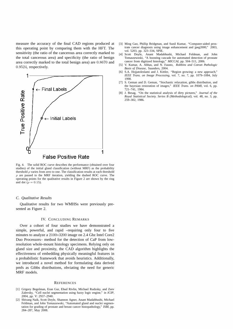
measure the accuracy of the final CAD regions produced atthis operating point by comparing them with the HFT. Thesensitivity (the ratio of the cancerous area correctly marked tothe total cancerous area) and specificity (the ratio of benignarea correctly marked to the total benign area) are0.8670 and0.9524, respectively.

Fig. 4. The solid ROC curve describes the performance (obtained over fourstudies) of the initial gland classification (without MRF) as the probabilitythresholdρ varies from zero to one. The classification results at each thresholdρ are passed to the MRF iteration, yielding the dashed ROC curve. Theoperating points for the qualitative results in Figure 2 areshown by the ringand dot (ρ = 0.15).

C. Qualitative Results

Qualitative results for two WMHSs were previously pre-sented as Figure 2.

IV. CONCLUDING REMARKS

Over a cohort of four studies we have demonstrated asimple, powerful, and rapid –requiring only four to fiveminutes to analyze a2100×3200 image on 2.4 Ghz Intel Core2Duo Processors– method for the detection of CaP from low-resolution whole-mount histology specimens. Relying onlyongland size and proximity, the CAD algorithm highlights theeffectiveness of embedding physically meaningful features ina probabilistic framework that avoids heuristics. Additionally,we introduced a novel method for formulating data derivedpmfs as Gibbs distributions, obviating the need for genericMRF models.

REFERENCES

[1] Grigory Begelman, Eran Gur, Ehud Rivlin, Michael Rudzsky, and ZeevZalevsky, “Cell nuclei segmentation using fuzzy logic engine,” in ICIP,2004, pp. V: 2937–2940.

[2] Shivang Naik, Scott Doyle, Shannon Agner, Anant Madabhushi, MichaelFeldman, and John Tomaszewski, “Automated gland and nuclei segmen-tation for grading of prostate and breast cancer histopathology,” ISBI, pp.284–287, May 2008.

[3] Ming Gao, Phillip Bridgman, and Sunil Kumar, “Computer-aided pros-trate cancer diagnosis using image enhancement and jpeg2000,” 2003,vol. 5203, pp. 323–334, SPIE.

[4] Scott Doyle, Anant Madabhushi, Michael Feldman, and JohnTomaszeweski, “A boosting cascade for automated detection ofprostatecancer from digitized histology,”MICCAI, pp. 504–511, 2006.

[5] V. Kumar, A. Abbas, and N. Fausto,Robbins and Cotran PathologicBasis of Disease, Saunders, 2004.

[6] S.A. Hojjatoleslami and J. Kittler, “Region growing: a new approach,”IEEE Trans. on Image Processing, vol. 7, no. 7, pp. 1079–1084, July1998.

[7] S. Geman and D. Geman, “Stochastic relaxation, gibbs distribution, andthe bayesian restoration of images,”IEEE Trans. on PAMI, vol. 6, pp.721–741, 1984.

[8] J. Besag, “On the statistical analysis of dirty pictures,” Journal of theRoyal Statistical Society. Series B (Methodological), vol. 48, no. 3, pp.259–302, 1986.