determinants of apanese yen interest …academic.udayton.edu/carlchen/research/jfm 2008.pdfyen...

DETERMINANTS OF JAPANESE

YEN INTEREST RATE SWAP

SPREADS: EVIDENCE FROM A

SMOOTH TRANSITION VECTOR

AUTOREGRESSIVE MODEL

YING HUANGCARL R. CHEN*MAXIMO CAMACHO

This study investigates the determinants of variations in the yield spreadsbetween Japanese yen interest rate swaps and Japan government bonds for a peri-od from 1997 to 2005. A smooth transition vector autoregressive (STVAR)model and generalized impulse response functions are used to analyze theimpact of various economic shocks on swap spreads. The volatility based on a GARCH (generalized autoregressive conditional heteroskedasticity) model ofthe government bond rate is identified as the transition variable that controls thesmooth transition from a high volatility regime to a low volatility regime. The break

We thank two anonymous reviewers and the editor, Bob Webb, for helpful comments. The views in this paperare those of the authors and do not represent the views of the Bank of Spain or the Eurosystem.

*Correspondence author: Department of Economics and Finance, University of Dayton, 300 College Park,Dayton, Ohio 45469–2251; e-mail: [email protected]

Received April 2006; Accepted February 2007

■ Ying Huang is an Assistant Professor in the Department of Economics and Finance atManhattan College in New York City, New York.

■ Carl R. Chen is the William J. Hoben Professor in the Department of Economics and Financeat the University of Dayton in Dayton, Ohio.

■ Maximo Camacho is a Fellow at the Bank of Spain and University of Murcia in Madrid,Spain.

The Journal of Futures Markets, Vol. 28, No. 1, 82–107 (2008)© 2008 Wiley Periodicals, Inc.Published online in Wiley InterScience (www.interscience.wiley.com).DOI: 10.1002/fut.20281

Yen Interest Rate Swap Spreads 83

Journal of Futures Markets DOI: 10.1002/fut

point of the regime shift occurs around the end of the Japanese banking crisis. Theimpact of economic shocks on swap spreads varies across the maturity of swapspreads as well as regimes. Overall, swap spreads are more responsive to theeconomic shocks in the high volatility regime. Moreover, a volatility shock has pro-found effects on shorter maturity spreads, whereas the term structure shock playsan important role in impacting longer maturity spreads. Results of this study alsoshow noticeable differences between the nonlinear and linear impulse responsefunctions. © 2008 Wiley Periodicals, Inc. Jrl Fut Mark 28:82–107, 2008

INTRODUCTION

This study provides an empirical examination of the dynamic behavior of theJapanese yen interest rate swap spreads1 (hereafter swap spreads) and relevantrisk factors within a smooth transition vector autoregressive (STVAR) frame-work. The nonlinear, state-dependent model better characterizes the Japaneseswap market since the late 1990s, and it uncovers asymmetric and regime-shifting movements in swap spreads.

Among the major players, Japanese yen interest rate swap plays a pivotalrole in the global interest rate derivatives market. It amounts to an average of15% of the total outstanding interest rate derivatives worldwide. The expansionin the Japanese yen interest rate swap speaks for the importance of under-standing the yen swap pricing mechanism. Surprisingly, few studies haveundertaken the task of seeking an appropriate explanation of the Japanese swapmarket dynamics.2

This research thus contributes to the literature in a number of aspects.First, the behavior of Japanese swap spreads is studied. Japanese swap spreadsare second in importance to its U.S. counterpart, yet they are much ignoredand understudied. Second, instead of using either a static single equationregression analysis or a linear vector autoregressive (VAR) model common inmost swap studies, we employ a smooth transition vector autoregressive (STVAR)model to examine the asymmetric effects of economic shocks on Japanese swapspreads. The nonlinear STVAR model allows for a smooth transition from oneregime of swap spreads to the other, controlled by an underlying economicdeterminant.

Third, the sample studied spans from 1997 to 2005, which not only offersthe most updated dataset, but also encompasses the Japanese banking crisis

1They are the spreads between Japanese yen interest rate swaps and Japanese government bonds with com-parable maturities.2To the best of our knowledge, so far only two studies have examined Japanese yen interest rate swaps. Oneis written in Japanese, which we could barely understand, and the other is an unpublished working paper(Eom, Subrahmanyam, and Uno, 2000), which uses data of an earlier period (1990–1996). Their sampleperiod is before the Japanese banking crisis and the subsequent extensive financial system reforms.

84 Huang, Chen, and Camacho


as well as a period of banking mergers and financial reforms. Thus, the study iswell positioned to investigate the swap market’s behavior under different mar-ket conditions. Indeed, the STVAR methodology identifies the existence of twoswap spread regimes, and the break point is around the end of the banking crisis.Using the latest data allows for the attainment of better-measured economic vari-ables, which are lacking in earlier years of the Japanese financial market.

In this study, sequential tests are performed to determine the best modelto employ. After that, within the nonlinear framework, the transition variableresponsible for the shift of regimes is identified to be the volatility variable basedon a GARCH (generalized autoregressive conditional heteroskedasticity) modelof the government bond rate. The transition function suggests that the firstregime is associated with periods of high volatility, whereas the second regimecorresponds to periods of low volatility, with the transition around the end ofthe Japanese banking crisis. Furthermore, generalized impulse response func-tions find that swap spreads of all maturities are more responsive to the eco-nomic shocks in the high volatility regime when Japan was going through abanking crisis. Differences in responses are also observed between the shorter-end and the longer-end of the swap maturity. Specifically, 2-year swap spreadsare more sensitive to the volatility shock than 5- or 10-year swap spreads, andmore pronounced effects after a shock originating from the slope of the termstructure are seen on longer maturity swap spreads in contrast to shorter matu-rity spreads. Finally, the implementation of an STVAR model over a linear VARensures sound results.

The rest of the article is organized as follows. In the next section, theissue of swap pricing is addressed and a literature review is provided alongwith a discussion of the determinants of swap spreads. Data sources andvariable definitions are presented in the third section. In the fourth section,statistical methodologies are discussed and empirical results are reported inthe fifth section. The conclusions are given in the final section.

SWAP PRICING, LITERATURE REVIEW, ANDDETERMINANTS OF SWAP SPREADS

Swap Pricing

A plain vanilla interest rate swap is a contractual agreement for one party topay a fixed rate (swap rate) in exchange for a stream of variable cash flowsbased upon a floating rate such as London Interbank Offered Rate (LIBOR) fora certain amount of notional principal. The interest rate that determines thefixed payment is the swap rate, and it is the interest rate that renders the valueof a swap contract to be zero at the initiation of the contract. Let F(t0, ti)



denotes the implied forward rate from time t0 to ti known at time 0 assuming nswap settlements on dates t0 to ti. Furthermore, the price of a default-free purediscount bond can be written as B(t0, ti), which represents the value of $1 to bereceived at time ti. Because floating-rate payments could be hedged using for-ward rate contracts, a hedged swap paying fixed rate, having zero netpresent value, requires that

(1)

Rearranging Equation (1), the swap rate is obtained as:

(2)

Therefore, swap rate, , can be regarded as a weighted average of the forward rate agreement paid-in-arrears rates3 during the life of the swap:

(3)

with the weight being

(4)

Because swap spread is measured by the difference between the swap rate,, and the government bond yield of equivalent maturity, arbitrage will ensure

a zero swap spread in a complete financial market. That is, an arbitrage-free value of the swap spread should be zero, implying that the swap rate shouldbe equal to the default-free par bond yield in the absence of market frictions. A non-zero swap spread is observed, however, when the financial markets areless than perfect, hence counterparty default risk exists. Because the swap spreadchanges over time, it is important to understand what drives the dynamics ofswap spread.

Literature Review

In recent years, researchers have begun to study the behavior of swap spreads.Modeling interest rate swaps as a party who is short an option to receive (pay)

St0

v �B(t0, ti)

an

i�1B(t0, ti�1)

St0� v1F(t0, t1) � # # # � vn�1F(t0, tn�1)

St0

St0�a

n

i�1B(t0,ti�1)F(t0,ti)

an

i�1B(t0,ti�1)

an

t�1B(t0, ti�1)[St0

� F(t0, ti)] � 0

St0,

3It is paid-in-arrears, because the unknown forward interest rate will be known at time t1 and the interestpayments are exchanged at time t2.



fixed and long an option to pay (receive) floating cash flows, with the counter-party simultaneously owning the opposite pair of options, Sorensen and Bollier(1994) argue that the value of a swap depends on the value of the option todefault. The value of the option to default, in turn, depends on a number offactors including the swap parties’ default probabilities, the shape of the yieldcurve, and interest rate volatility. Swap spreads, therefore, are partially deter-mined by the default risk, which may be associated with the interest ratevolatility and the term structure of the interest rate.

Grinblatt (2001), however, advances that generic swaps are default-free,and he attributes the swap spread to the liquidity differences between govern-ment securities and Eurodollar borrowings. Specifically, he contends that swapspreads contain a convenience yield (liquidity premium) not available in themore liquid government securities. Increases in liquidity premium, therefore,imply that the market requires a higher premium to compensate for thereduced liquidity, which should result in a corresponding increase in the swapspread. Collin-Dufresne and Solnik (2001), and He (2000) echo the sameargument because the net interest payment streams involved in the swap aremuch smaller than in a bond.

Empirical evidence to date is far from conclusive. Minton (1997) findsthat bilateral counterparty default risk measured by corporate quality spread isnot statistically related to the swap rate. However, unilateral default risk meas-ured by aggregate default spread, exerts significant and positive impact on swaprate. Using VAR analyses, Huang and Neftci (2006) find that liquidity risk, notdefault risk, is the primary driver of U.S. interest rate swap spreads. Liu,Longstaff, and Mandell (2006) report that the risk of changes in the defaultprobability is virtually not priced by the market. On the other hand, employingimpulse response function and variance decomposition method, Duffie andSingleton (1997) conclude that both credit and liquidity risks have an impacton the U.S. swap zero spread, although the swap spread’s own innovationaccounts for the majority of the spread’s variations. Other studies examiningthe impact of liquidity and default risk premiums on swap spreads includeBrown, Harlow, and Smith (1994), Lang, Litzenberger, and Liu (1998), Sun,Sudaresan, and Wang (1993), and Fehle (2003). In addition to default and liq-uidity premiums, other economic determinants of swap spreads in prior studiesconsist of interest rate volatility and slope of the yield curve as they are alterna-tive proxies of financial market risks (e.g., In, Brown, & Fang, 2003; Lekkos &Milas, 2001, 2004).

Although most of the studies focus on the U.S. swap rates and spreads,few examine interest rate swaps of other currencies. Suhonen (1998) considersthe determinants of swap spreads in Finland and finds that spreads are posi-tively related to the slope of the yield curve and interest rate volatility. Lekkos



and Milas (2001) study interest rate swaps using both U.S. and U.K. data.Lekkos and Milas (2004) model U.S. and U.K. swap spreads within an STVARframework allowing for steep or flat yield curve slopes. Fang and Muljono(2003) investigate Australian dollar interest rate swaps and conclude that thespreads mostly represent a credit risk premium. In an unpublished workingpaper, Eom, Subrahmanyam, and Uno (2000) study the credit risk and theJapanese yen interest rate swap during the period of 1990–1996. They find thatyen swap spreads behave very differently from the credit spreads on Japanesecorporate bonds, and overall the yen swap market is sensitive to credit risk.Their study, however, only presents evidence on a period that is before theJapanese banking crisis and subsequent financial system reforms. Importantly,the majority of the swap rate studies rely upon ordinary least squares (OLS)and linear VAR analyses. Nonlinear models in recent years have been proven tooutperform the linear ones, such as Lekkos and Milas (2004) and Milas,Lekkos, and Panagiotidis (2007), which find interpretation of the results moreflexible and provide better predictive power on swap spreads.

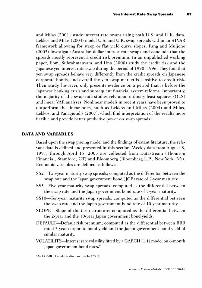
DATA AND VARIABLES

Based upon the swap pricing model and the findings of extant literature, the rele-vant data is defined and presented in this section. Weekly data from August 8,1997, through April 15, 2005 are collected from Datastream (ThomsonFinancial, Stamford, CT) and Bloomberg (Bloomberg L.P., New York, NY).Economic variables are defined as follows:

SS2—Two-year maturity swap spreads; computed as the differential between theswap rate and the Japan government bond (JGB) rate of 2-year maturity.

SS5—Five-year maturity swap spreads; computed as the differential betweenthe swap rate and the Japan government bond rate of 5-year maturity.

SS10—Ten-year maturity swap spreads; computed as the differential betweenthe swap rate and the Japan government bond rate of 10-year maturity.

SLOPE—Slope of the term structure; computed as the differential betweenthe 2-year and the 10-year Japan government bond yields.

DEFAULT—Default risk premium; computed as the differential between BBBrated 5-year corporate bond yield and the Japan government bond yield ofsimilar maturity.

VOLATILITY—Interest rate volatility fitted by a GARCH (1,1) model on 6-monthJapan government bond rates.4

4An EGARCH model is discussed in In (2007).



LIQUIDITY—Liquidity premium; computed by subtracting 6-month Japangovernment bond rates from 6-month Japanese yen Tokyo InterbankOffered Rate (TIBOR).

JAPAN PREMIUM—the spread between TIBOR and LIBOR on Japaneseyen.

Prior studies are followed in terms of measuring default risk. For example,Minton (1997) uses corporate quality spread (BAA�AAA) and aggregatedefault spread (BAA�T-Bond) to measure counterparty default risk. Duffie andSingleton (1997) use the spread between BAA- and AAA-rated commercialpaper rates, and Huang and Neftci (2006) use the TED (T-bill/Eurodollar)spread to measure credit risk. In a similar fashion, yield data on Japanese gov-ernment bonds (JGB), AAA-rated, and BBB-rated corporate bonds has beencollected for this study. However, because AAA-rated bonds have a significantquantity of missing data, the spread between BBB-rated corporate bonds andJGB yields is employed to proxy the default premium.

The interest rate volatility generated by a GARCH model and the slope ofthe term structure of interest rates are also included in our empirical modelbecause these two variables determine the value of the option to default in theSorensen and Bollier’s (1994) model. Because increasing interest rate volatilityis often associated with economic uncertainty, as such, it is expected to posi-tively influence swap spreads. Theoretically, the impact of the slope of the termstructure on swap spreads could be either positive or negative. For instance,according to Sorensen and Bollier (1994), when the yield curve is upward slop-ing, the fixed payer (floating receiver) is exposed to higher counterparty riskdue to higher default risk exposure associated with the higher future floatingpayments. A lower fixed swap rate will compensate for this increased risk. Swapspreads are thus expected to be negatively related to the slope of the termstructure. On the other hand, upward sloping yield curve normally coincideswith strong economic growth, during which bond credit premium tends tobecome larger (Alworth, 1993). In this case, swap spreads are expected to bepositively related to the slope of the term structure.

Following Grinblatt (2001), the liquidity premium is measured by sub-tracting 6-month JGB yield from a similar maturity TIBOR rate. Becauseincreasing convenience yield implies that the market requires a higher premi-um to compensate for the decrease of liquidity in the TIBOR market, liquiditypremium is also expected to be positively associated with swap spreads. Thevariable JAPAN PREMIUM, computed as the spread between 6-monthTIBOR and LIBOR, is chosen to represent international financial markets’assessment of risks unique to Japan. During the period of Japanese banking



crisis, Japanese banks borrowing U.S. dollars must pay a significant amount ofpremium.

Figure 1 provides plots of the above variables. Swap spreads are generallyhigher and more volatile before 2001, and the term structure of swap spreads isupward sloping with 10-year spreads the highest. There are also periods when2-year spreads become negative. After 2001, however, swap spreads are lower,less volatile, and the term structure of swap spreads becomes inverted with 2-year and 5-year swap spreads higher than the 10-year spreads. The periods ofhigher and more volatile swap spreads coincide with the era that Japaneseeconomy went through a recession and banking crisis. In late 1997, severalreputable security firms including Sanyo Securities, Hokkaido TakushokuBank, Yamaichi Securities, and Tokuyo City Bank, announced the closure oftheir business in a single month. Although the onset of the banking system trou-ble began in 1994 when credit cooperatives and housing finance companies( Jusen) encountered serious financial problems, the unprecedented collapse ofmajor banks propagated the rumors and shook the confidence of the entireJapanese financial system. The credit ratings of banking firms rapidly degenerat-ed during this period such that the term Japan Premium, a premium on lendingto Japanese institutions, appeared in the international financial markets. In theplot of JAPAN PREMIUM, it is obvious that larger premiums predominatelyappear in the periods of the late 1990s. By late 2000, the new capital injectionguided by the Financial Function Strengthening Law seemed to have restoredconfidence in Japanese banks, hence the decline in premiums. The magnitudeof the premiums reduces to less than five basis points during the postbankingcrisis period.5

Shown in the plot of VOLATILITY, volatilities are also much higher before2001, but become minuscule after that. Interestingly, liquidity premiums alsoshow similar patterns. Before 2001, liquidity premiums are generally higher andmore volatile, but hovering around 10 basis points afterwards. Default premi-ums display those patterns alike, although not as dramatic as the other econom-ic determinants of swap spreads. The only variable that does not exhibit a strongpattern is the slope of the JGB term structure. Most of the time, the slope moveswithin a range between 100 and 160 basis points, with two exceptions when itdips below 50 basis points.

Table I presents descriptive statistics of the economic variables employedin this study. Panel A shows the statistics for the whole sample. It can be seenthat the term structure of swap spreads is upward sloping with SS10 the high-est at 15.4 basis points, SS5 at 11.7 basis points, and SS2 the lowest at 8 basis

5For detailed discussions of the Japanese banking crisis, see Nakaso (2001), Miyajima and Yafeh (2003), andKrawczyk (2004).



�.4

�.2

.0

.2

.4

.6

.8

1998 1999 2000 2001 2002 2003 2004

10YR spread 2YR spread 5YR spread

1997 2005

DEFAULT

0

1

2

3

4

5

6

1997 1998 1999 2000 2001 2002 2003 2004 2005

1997 1998 1999 2000 2001 2002 2003 2004 2005

1997 1998 1999 2000 2001 2002 2003 2004 2005

1997 1998 1999 2000 2001 2002 2003 2004 2005

1997 1998 1999 2000 2001 2002 2003 2004 2005

JAPAN PREMIUM

�0.2

�0.1

0

0.1

0.2

0.3

0.4

0.5

LIQUIDITY

0

0.1

0.2

0.3

0.4

0.5

0.6

0.7

0.8

0.9SLOPE

0.2

0.4

0.6

0.8

1

1.2

1.4

1.6

1.8

VOLATILITY

0

0.2

0.4

0.6

0.8

1

FIGURE 1Plots of swap spreads and economic determinants.



points. Considering the Japanese economic conditions, the ex post patterns ofswap spreads and their economic determinants discussed above, the wholesample is further partitioned into two subperiods. Panel B shows the statisticsfor the subperiod between August 1997 and December 2000; Panel C presentsthe same statistics for the second subperiod between January 2001 and April2005.6 Consistent with Figure 1, the default premium, the Japan premium, theliquidity premium, and volatility are larger and more volatile (higher standarddeviations) in the first subperiod, reflecting the impact of the banking crisis.For swap spreads, both SS10 and SS5 are significantly higher in period 1.Average SS10 is 31 basis points in period 1, but is less than 3 basis points inperiod 2—a 10-fold difference. For the shorter-maturity swap spread (SS2), themean spreads are nearly identical in the two subperiods. These preliminary sta-tistics seem to suggest that longer-maturity swap spreads are more sensitive tochanging economic conditions.

6This preliminary sample partitioning for descriptive statistics in fact coincides with the test results of theregime shift reported in Section 5.

TABLE I

Descriptive Statistics

DEFAULT JPPREM LIQUIDITY SLOPE SS10 SS5 SS2 VOLATILITY

Panel A: Whole sampleMean 1.524 0.051 0.169 1.197 0.154 0.117 0.081 0.129Median 1.473 0.028 0.098 1.241 0.093 0.101 0.081 0.027Maximum 4.995 0.417 0.876 1.683 0.596 0.496 0.316 0.705Minimum 0.467 �0.098 0.039 0.400 �0.086 �0.077 �0.220 0.000SD 0.739 0.071 0.152 0.245 0.161 0.091 0.074 0.158

Panel B: 1997–2000

Mean 1.946 0.085 0.267 1.225 0.312 0.172 0.079 0.272Median 1.944 0.041 0.204 1.236 0.323 0.201 0.075 0.251Maximum 4.995 0.417 0.876 1.683 0.596 0.496 0.316 0.705Minimum 0.755 �0.098 0.039 0.407 �0.027 -0.077 -0.220 0.049SD 0.794 0.096 0.188 0.248 0.097 0.099 0.109 0.137

Panel C: 2001–2005

Mean 1.189 0.023 0.095 1.174 0.029 0.073 0.083 0.015Median 1.151 0.022 0.091 1.247 0.021 0.063 0.082 0.007Maximum 2.102 0.086 0.236 1.624 0.214 0.242 0.168 0.185Minimum 0.467 �0.011 0.066 0.400 �0.086 -0.053 0.029 0.000SD 0.476 0.015 0.022 0.242 0.059 0.051 0.021 0.026

Notes. This table displays the descriptive statistics of swap spreads and their economic determinants. SS2, SS5, andSS10 are swap spreads of 2-year, 5-year, and 10-year maturities, respectively. DEFAULT is the default premium, JPPREMis the Japan premium, LIQUIDITY is the liquidity premium, SLOPE is the slope of the term structure of government bonds,and VOLATILITY is the interest rate volatility generated by a GARCH model.



METHODOLOGY

The Baseline Model

Because the sampling period used in this study encompasses different economicregimes, a linear VAR may not be the appropriate model to use. In this section,the VAR extension of the STVAR model in Camacho (2004) is considered,which is also employed in Lekkos and Milas (2004), and Milas et al. (2007).The model permits a smooth transition of regimes based upon an empiricallychosen economic factor. Let

Yt � A � B(L)Yt�1 � (C � D(L)Yt�1)F(Yi,t�d) � ut, (5)

where Yt represents a time-series vector including swap spreads (SS2, SS5, orSS10), slope of the term structure (SLOPE), default premiums (DEFAULT),liquidity premiums (LIQUIDITY), Japan premiums (JAPAN PREMIUM), andinterest rate volatilities (VOLATILITY). A and C are vectors of intercepts,B(L) and D(L) are polynomial matrices of pth order lag, d is the delay param-eter, and ut follows an independent and identically distributed Gaussianprocess with zero mean and variance �.

The key component of this STVAR system is the transition function F(•),which controls the regime switching and is bounded between zero and one.When F(•) is zero, Equation (5) becomes a linear VAR (VAR-a) with parame-ters A and B(L). On the contrary, when F(•) is one, the model becomes a dif-ferent linear VAR (VAR-b) with parameters A � C and B(L) � D(L). Hence,F(•) may be interpreted as a filtering rule that locates the model between thesetwo extreme regimes. Until these regimes can be interpreted economically, theywill be referred to as first regime and second regime, respectively.

To consider different forms of transition across these regimes, two transi-tion functions have been developed in the literature. The first one is the logisticfunction, stated as:

F(Yi,t�d)�{1� exp[��(Yi,t�d�c)]/�}�1, (6)

where c is the threshold between two regimes, and s is the standard deviation ofYi,t � d. The second one is the exponential transition function, which can be writ-ten as:

F(Yi,t�d)�1� exp[��(Yi,t�d �c)2]/�2]. (7)

When the transition function F(Yi,t�d) is set to be logistic, it changes monoton-ically from the first regime to the second regime with transition value Yi,t�d.The transition function becomes a constant when � ➝ 0, and the transitionfrom 0 to 1 is instantaneous at Yi,t�d � c when � ➝ ��. On the other hand,



under the exponential function, the system changes symmetrically relative to thethreshold c with Yi,t � d, but the model turns linear if either � ➝ 0 or � ➝ ��. Inboth models, the smoothness parameter �, which is restricted to be positivebetween zero and one, controls the speed of adjustment across regimes.

Linearity Tests and the Transition Function

We follow the specification suggested in Camacho (2004), which adapts theunivariate proposal of Granger and Teräsvirta (1993) to a multiequation con-text, for the empirical examination of the behavior of Japanese Yen swapspreads.

The first step of the estimation is to specify a linear VAR model as the basisto obtain the nonlinear results. This is because even if the true model is non-linear, the linear specification is a simpler framework to obtain preliminaryresults that may assist in obtaining the set of variables to include in the nonlin-ear specification. In a small-scale system, linear specification may also help usto decide the maximum lag length p. In a large-scale system, however, theselection of p may be constrained to consider a tractable number of parametersto be estimated. Because our system contains six variables, we restrict ouranalysis to VAR models of order one. Estimations based upon higher orderVARs have also been tried but they fail to converge in the nonlinear models.

Next, some linearity and model selection tests are conducted. The max-imum likelihood method is employed for the estimation, in which (2� thelog-likelihood under the alternative—the log-likelihood under the null) willfollow asymptotically a 2 distribution with degrees of freedom equal to thenumber of restrictions imposed under the null.7

Assuming that d is known, testing linearity is still nonstandard due to thepresence of nuisance parameters. Following the suggestions of Luukkonen,Saikkonen, and Teräsvirta (1988), the problem may be overcome by suitableTaylor approximations of the transition function around � � 0. Assuming p � 1,the problem of testing linearity is reduced to estimating the following auxiliaryregression:

(8)

for each transition variable candidate i � 1, 2, . . . , 6, and to test

H0: G1 � G2 � G3 � 0.

In empirical applications, d is usually restricted to be less than or equal to p,therefore, just one lag is considered for each candidate of the transition variable.

Yt�g�G0Yt�1 � G1Yt�1Yi,t�d � G2Yt�1Yi,t�d2 � G3Yt�1Yi,t�d

3 � et

7See Camacho (2004) for technical details about maximum likelihood estimation.



Linearity tests are applied for each of these lagged variables. In case of multiplerejections of the null, we follow Teräsvirta (1994) such that the lagged variablewith the highest rejection of linearity (i.e., the largest statistic or the lowest p-value) is chosen as the most suitable transition variable.

The results of the linearity tests appear in Table II. The null of linearity isessentially rejected in all variables with the exception of lagged swap spreads inthe SS5 model. Hence, it confirms that a nonlinear model better fits ourJapanese swap data. The following step is to choose the transition variable. Toselect just one transition variable that is responsible for the regime shift in thenonlinear model, the ratio of the linearity test statistic is also shown for eachcandidate over the statistic that corresponds to VOLATILITY, which has thelargest statistic across all spread maturities. Accordingly, lagged volatility isadopted as the transition variable in the transition function.

After determining the delay parameter d and the transition variable thatgoverns the transition across regimes, the third step is to choose between alogistic and an exponential form of the transition function. The tests that are

TABLE II

Linearity Tests and Identification of Transition Variable

Transition variable candidates (in t-1)

SS DEFAULT JPPREM LIQUIDITY SLOPE VOLATILITY

SS2 Test 136.58 161.36 206.48 345.18 357.71 385.11model statistics

(p-value) (0.032) (0.007) (0.000) (0.000) (0.000) (0.000)Test 0.355 0.419 0.536 0.896 0.929 1.000statisticsratio


(p-value) (0.115) (0.001) (0.000) (0.000) (0.000) (0.000)Test 0.303 0.382 0.449 0.941 0.964 1.000statistics ratio


(p-value) (0.006) (0.002) (0.001) (0.000) (0.000) (0.000)Test 0.297 0.313 0.321 0.940 0.964 1.000statistics ratio

Notes. This table reports linearity test results and the identification of a transition variable that controls the regime shift. Test statistics along with the corresponding p-values for each swap maturity are reported. The ratios of the test statis-tic for each transition variable candidate over the test statistic for the lagged volatility are also shown. SS denotes swap spreads, DEFAULT is the default premium, JPPREM is the Japan premium, LIQUIDITY is the liquidity premium,SLOPE is the slope of the term structure of government bonds, and VOLATILITY is the interest rate volatility generated bya GARCH model.



sequentially applied to the auxiliary regression (i.e., H01, H02, and H03, respec-tively) and subsequent decisions are illustrated in Table III. Using lagged volatilityas the transition variable, the p-values of Test 1, Test 2, and Test 3 are all about0.000. Therefore, the appropriate transition function is logistic.

EMPIRICAL RESULTS

Regime Identification

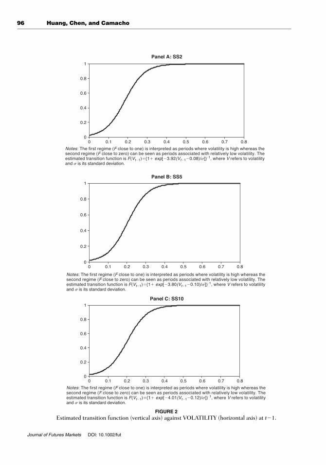
The logistic transition function model is now estimated using the maximum like-lihood method.8 For the ease of presentation and to shed some light on thenonlinearities obtained in the model, Figure 2 plots the transition functionagainst lagged volatility for all swap maturities. The estimates of the speed oftransition (�) between regimes and the threshold parameter (c) are also report-ed in the notes under each panel. The transition function suggests that the firstregime (F close to one) is associated with periods of high volatility, whereas the second regime (F close to zero) is classified as the low volatility regime. Theestimated threshold levels (c) are about 0.08, 0.10, and 0.12, which mark the halfway point between regimes, for SS2, SS5, and SS10 respectively. Theestimated smoothness parameters (�), which determine the velocity of transi-tion between these two states, are close to 4 for all swap maturities with minorvariations.

Figure 3 plots the values of the transition function (solid line, left-hand axis)and VOLATILITY (line with blocks, right-hand axis) for all swap maturities. It isclearly shown that high values of the transition function F are associated with

TABLE III

Functional Form of the Transition Function

Test 1 Test 2 Test 3

H01: G3�0 H02: G2�0/G3�0 H03: G1�0/G3�G2�0

Results Decision

Reject N/A N/A LogisticAccept Reject Accept ExponentialAccept Accept Reject LogisticAccept Reject Reject No decision

Notes. This table reports test results of selecting the transition function using lagged volatility asthe transition variable. The decisions on the choice between a logistic and an exponential modelare indicated in the last column. Using lagged volatility as the transition variable, the p-valuesof Test 1, Test 2, and Test 3 are all about 0.000. Therefore, we conclude that the appropriatetransition function is logistic.

8Parameter estimates are not reported to save space. They are available from the authors upon request.



Panel A: SS2

Panel B: SS5

0

0.2

0.4

0.6

0.8

1

0

0.2

0.4

0.6

0.8

1

0 0.1 0.2 0.3 0.4 0.5 0.6 0.7 0.8

0 0.1 0.2 0.3 0.4 0.5 0.6 0.7 0.8

0

0.2

0.4

0.6

0.8

1

0 0.1 0.2 0.3 0.4 0.5 0.6 0.7 0.8

Notes: The first regime (F close to one) is interpreted as periods where volatility is high whereas the second regime (F close to zero) can be seen as periods associated with relatively low volatility. The estimated transition function is F(Vt�1)�{1� exp[�3.92(Vt�1�0.08)/�]}�1, where V refers to volatility and � is its standard deviation.



Panel C: SS10

FIGURE 2Estimated transition function (vertical axis) against VOLATILITY (horizontal axis) at t�1.



Notes: The transition function is the solid line (left-hand axis) and volatility is the line with blocks (right-hand axis). Values of the transition function close to one refer to the first regime and correspond to periods of high volatility. Note that the break point is at about the end of the banking crisis, a time period characterized with rapid reduction in volatility.

Panel A: SS2

Panel B: SS5

1997 1998 1999 2000 2001 2002 2003 2004 2005

Panel C: SS10

0

0.2

0.4

0.6

0.8

1

0

0.2

0.4

0.6

0.8

1

1997 1998 1999 2000 2001 2002 2003 2004 20050

0.2

0.4

0.6

0.8

1

0

0.2

0.4

0.6

0.8

1

1997 1998 1999 2000 2001 2002 2003 2004 20050

0.2

0.4

0.6

0.8

1

0

0.2

0.4

0.6

0.8

1

FIGURE 3Transition function and VOLATILITY.



occurrence of high volatility from 1997 to 2000. From 2001 to 2005, however,the transition function falls dramatically to almost zero which corresponds to along period of low volatility. It should be noted that the break point betweenregimes occurs near the end of the Japanese banking crisis.

Generalized Impulse Response Analysis

In this subsection, the estimation procedure of the generalized impulseresponse function (GIRF) is explained, and associated empirical results for theSTVAR models are reported. Because impulse responses identify the conse-quences of an increase in the jth variable innovation at date t for the value ofthe ith variable at time t � h, the GIRF of the STVAR model traces the timepath where the swap spread returns to equilibrium after an economic shock isinjected into the system. The visual aids provided by the impulse responsefunctions are particularly useful when the full impact of economic shocks onswap spreads takes long lags to materialize.

In the nonlinear context, however, these effects not only depend on theshocks that occur between t and t � h, but also on the past shock history, wt�1.Following Weise (1999), the generalized impulse response function of variablei for an arbitrary shock to variable j denoted by jt � dj and history wt�1 isdefined as:

GIRF(h,dj , wt�1) � E(Yi,t�h/jt � dj, wt�1) � E(Yi,t�h/ wt�1). (9)

In the empirical application, �j is set to one standard deviation of variable j.In other words, the shock to each equation is equal to one standard deviation ofthe equation residual. Note that, in linear contexts, shocks between t and t � hare usually set to zero for convenience. As documented by Koop, Pesaran, andPotter (1996), this approach is not appropriate in the context of nonlinear models.9

To deal with the problem of shocks in intermediate time periods, the bootstrapprocedure suggested by Weise (1999) is followed. First, we obtain 5,000 drawswith replacements from the residuals of the nonlinear model, compute theGIRF for each of them, and then average the responses. In addition, GIRFs arehistory dependent. To account for this dependency, the GIRFs are computed

9In linear models, impulse responses of variable i to shocks in variable j can be defined as the differencebetween realizations of Yi,t�h and a baseline “no shock” scenario:

IRF(h, dj, wt�1) � E(Yi,t�h/jt�dj,jt�1�0,...,jt�h�0,wt�1) � E(Yi,t�h|ejt � 0,..., ejt+h � 0, wt�1)

where d is set to one standard deviation of variable j. Note that all shocks in intermediate periods between tand t � h are set equal to zero. This is because the expectation of the path of Y following a shock, conditionalon the future shocks, is equal to the path of the variable when future shocks are set to their expected values.Therefore, future shocks can be set equal to zero for convenience.



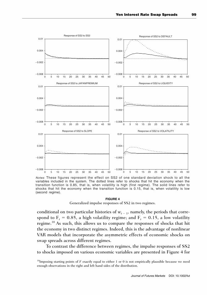
conditional on two particular histories of wt � 1, namely, the periods that corre-spond to Ft � 0.85, a high volatility regime; and Ft � 0.15, a low volatilityregime.10 As such, this allows us to compare the responses of shocks that hitthe economy in two distinct regimes. Indeed, this is the advantage of nonlinearVAR models that incorporate the asymmetric effects of economic shocks onswap spreads across different regimes.

To contrast the difference between regimes, the impulse responses of SS2to shocks imposed on various economic variables are presented in Figure 4 for

10Imposing starting points of F exactly equal to either 1 or 0 is not empirically plausible because we needenough observations in the right and left hand sides of the distribution.

Response of SS2 to SS2

0.008

0.002

0.004

0.01

0 5 10 15 20 25 30 35 40 45 500.008

0.002

0.004

0.01

0 5 10 15 20 25 30 35 40 45 50

0.008

0.002

0.004

0.01

0 5 10 15 20 25 30 35 40 45 500.008

0.002

0.004

0.01

0 5 10 15 20 25 30 35 40 45 50

0.008

0.002

0.004

0.01

0 5 10 15 20 25 30 35 40 45 500.008

0.002

0.004

0.01

0 5 10 15 20 25 30 35 40 45 50

Response of SS2 to DEFAULT

Response of SS2 to JAPANPREMIUM Response of SS2 to LIQUIDITY

Response of SS2 to SLOPE Response of SS2 to VOLATILITY

Notes: These figures represent the effect on SS2 of one standard deviation shock to a l l the variables included in the system. The dotted lines refer to shocks that hit the economy when the transition function is 0.85, that is, when volatility is high (first regime). The solid lines refer to shocks that hit the economy when the transition function is 0.15, that is, when volatility is low (second regime).

FIGURE 4Generalized impulse responses of SS2 in two regimes.



the high and low volatility regimes. Several dissimilarities between regimesstand out. First, swap spreads are generally more responsive to economicshocks in the high volatility regime. For example, in the first regime a shock ondefault premium generates a positive impact on SS2, which peaks at approxi-mately one basis point in week seven, and the impact gradually dies out inabout 40 weeks. A similar shock in the second regime only provokes a responseless than 0.4 bps from SS2. Although differing in magnitude, the positiveimpact of default shock on swap spreads is consistent with a priori expectations.

Similar observations can be found in swap spreads from a shock emanat-ing from volatility. SS2 reacts stronger to a volatility shock in the first regimethan in the second. The positive response of SS2 peaks out at 0.4 bps in about5 weeks, leveling off in about 35 weeks in the high volatility regime. By con-trast, in the low volatility regime, the response is merely less than half of the response in the first regime and rapidly disappears in about 5 weeks. Theimpulse response of SS2 to the term structure shock also displays an asymmet-ric pattern. A positive, though small response is observed in the first regime,which is in agreement with the findings reported in Alworth (1993) for the U.S.dollar swap spreads, and Suhonen (1998) for Finland data. The swap spread’sresponse to the term structure shock, however, is virtually nil in the secondregime. The responses of SS2 to liquidity premium and Japan premium alsoexhibit regime-dependent, asymmetric patterns, although not as dramatic asthose that are invoked by shocks from default premium and volatility. Theeffects of swap spreads from the shock in Japan premium are by far the smallestamong all.

In a similar fashion, the impulse responses of SS5 and SS10 to the eco-nomic shocks in different regimes are presented in Figures 5 and 6, respectively.Again, swap spreads appear to be more responsive to economic shocks when thehigh volatility regime dominates, and no significant responses are uncovered inthe low volatility regime.

Our model also successfully captures differential responses in swapspreads across different maturities. The impulse response results for SS5 in the high volatility regime are used to illustrate these differences. First, theresponse of swap spreads to the default shock is more pronounced for the shorter-term swap (i.e., SS2). The peak response of SS2 to default shock isone bp, whereas it is approximately half of this magnitude for SS5. Similareffects are also revealed in the results for the volatility shock, where SS2 is moreresponsive to the volatility shock than SS5. Conversely, the response of SS5 tothe term structure shock, the opposite is true. That is, the magnitude of theresponse of SS5 to the default shock is twice that of SS2. This is similar to the findings in other studies (e.g., Lekkos & Milas, 2004). This result stems fromthe fact that the exposure to the possibility of default (from the floating-rate



payer in the swap deal) for the fixed rate payer is higher during the later stageof the contract, hence higher embedded risks for the longer-term contracts.

In terms of 10-year swap spreads, the difference in responses due to maturi-ties is particularly manifest in shocks from default, liquidity, and term structureslope risks. Other than default shocks, responses of SS10 to shocks emanatingfrom other variables more resemble those of SS5 than SS2. Distinct from shorter-maturity swap spreads, in the high volatility regime SS10 initially declines fol-lowing a default shock, but the response reverts to be positive 7 weeks there-after. This result seems to be somehow related to Eom et al.’s (2000) finding ofa negative covariance between the default-free rate and the swap spread in Japan


0.008

0.002

0.004

0.01

0 5 10 15 20 25 30 35 40 45 50


0.008

0.002

0.004

0.01

0 5 10 15 20 25 30 35 40 45 50

Response of SS5 to JAPANPREMIUM

0.008

0.002

0.004

0.01

0 5 10 15 20 25 30 35 40 45 50

Response of SS5 to LIQUIDITY

0.008

0.002

0.004

0.01

0 5 10 15 20 25 30 35 40 45 50

Response of SS5 to SLOPE

0.008

0.002

0.004

0.01

0 5 10 15 20 25 30 35 40 45 50

Response of SS5 toVOLATILITY

0.008

0.002

0.004

0.01

0 5 10 15 20 25 30 35 40 45 50





during this period. Our result may be consistent with their finding if the correlationbetween BBB-bond yields and JGB yields is positive.11

Comparison of Nonlinear and Linear ImpulseResponse Functions

In this subsection, it is shown that results differ substantially between linearand nonlinear models. To save space, Figures 7 and 8 only exhibit the impulseresponses of swap spreads to default shocks and spreads’ own shocks. In Panel A


0.008

0.002

0.004

0.01

0 5 10 15 20 25 30 35 40 45 50


0.008

0.002

0.004

0.01

0 5 10 15 20 25 30 35 40 45 50

Response of SS10 to JAPANPREMIUM

0.008

0.002

0.004

0.01

0 5 10 15 20 25 30 35 40 45 50

Response of SS10 to LIQUIDITY

0.008

0.002

0.004

0.01

0 5 10 15 20 25 30 35 40 45 50

Response of SS10 to SLOPE

0.008

0.002

0.004

0.01

0 5 10 15 20 25 30 35 40 45 50

Response of SS10 to VOLATILITY

0.008

0.002

0.004

0.01

0 5 10 15 20 25 30 35 40 45 50



11We also run an OLS regression with all economic determinants and lagged SS10 (one lag) as the exogenousvariables to ensure that our finding is not methodology-driven. The OLS results show a negative relationbetween default premium and swap spreads during this sample period.



�0.008

�0.002

0.004

0.01

0 5 10 15 20 25 30 35 40 45 50

�.010

�.005

.000

.005

.010

5 10 15 20 25 30 35 40 45 50

�.010

�.005

.000

.005

.010

5 10 15 20 25 30 35 40 45 50

Panel A. Nonlinear model; first regime

Panel B. Linear model; whole sample

Panel C. Linear model; first regime

FIGURE 7Comparison of linear and nonlinear impulse responses of SS2 to default shock.



of Figure 7, the response of SS2 to default shock in the high volatility regimefrom the nonlinear model is presented for contrasting purpose. Panel B plotsthe response of SS2 to default shock in a linear model for the entire samplefrom 1997 to 2005 without considering the shift in regimes. The two panelsreveal drastic differences in impulse responses. The significant impact ofdefault shock on SS2 in the nonlinear model is completely absent in the linearmodel. Panel C indicates that the linear model also fails to capture the acuteresponse of SS2 to default shock during the first regime.

In Figure 8, the responses of SS5 to its own shock based upon nonlinearand linear models are illustrated. In Panel A, the high volatility regime witnessesa rather short-lived, diminutive reaction of SS5 to its own shock in the nonlin-ear model. However, the linear model depicted in Panel B demonstrates that forthe whole sample the long-lasting impact does not die out until 30 weeks later.Evident in Panel C, the linear impulse response of SS5 to its own shock underthe first regime suggests that the effect persists over a long horizon. TheSTVAR results thus help us avoid any fallacious conclusions due to a linearmodel specification.

CONCLUSIONS

In this article, the nonlinear relationships of Japanese yen interest rate swapspreads and a number of risk factors within a smooth transition VAR frame-work are modeled. Weekly data for the 2-year, 5-year, and 10-year swap spreadsand corresponding economic determinants of swap spreads, namely defaultpremium, liquidity premium, the term structure slope, Japan premium, andinterest rate volatility, are obtained from 1997 to 2005 for this purpose. Thisnonlinear model captures a time-varying component of swap spreads across dif-ferent maturities. The nonlinear dynamics are corroborated by the fact thatswap spreads of all maturities are very volatile and large in magnitude duringthe period of the Japanese banking crisis, but become much smaller and morestable during the post-banking crisis period. Most of the swap spread determi-nants exhibit signs of a regime shift as well.

Linearity tests reject the linear model in favor of a nonlinear VAR, and the model selection tests conclude that a logistic transition function better fits thedata. Interest rate volatility is identified as the transition variable responsible forthe shift of regimes. The estimated transition function suggests that the firstregime is associated with periods of high volatility, whereas the second regimecorresponds to periods of low volatility. Incidentally, this break point occurs nearthe end of the Japanese banking crisis.

Generalized impulse response functions help analyze the time paths of theimpact of economic shocks on swap spreads of various maturities across



�0.008

�0.002

0.004

0.01

0 5 10 15 20 25 30 35 40 45 50

�.10

�.05

.00

.05

.10

5 10 15 20 25 30 35 40 45 50

�.10

�.05

.00

.05

.10

5 10 15 20 25 30 35 40 45 50

Panel A. Nonlinear model; first regime

Panel B. Linear model; whole sample

Panel C. Linear model; first regime

FIGURE 8Comparison of linear and nonlinear impulse responses of SS5 to own shock.



regimes. Three major conclusions are in order. First, a regime effect is presentduring the period we study. Swap spreads of all maturities are more responsiveto economic shocks in the high volatility regime when Japan was going througha banking crisis. It is found that the magnitude of the peak response of SS2 todefault and volatility shocks in the high volatility regime is more than twice ofthat in the low volatility regime. The corresponding response of SS2 to a termstructure shock can be hardly detected in the second regime. Second, a matu-rity effect is implied in the variability of swap spreads across regimes.Dissimilarities in responses are observed between the short-end of the swapmaturity (SS2) and the longer-end (SS5 and SS10). It is evident from our esti-mation that SS2 is more responsive to the volatility shock than SS5 or SS10.Impulse responses of swap spreads to the term structure shock exhibit an oppo-site pattern, with longer maturity swaps more sensitive. This finding is consistentwith the notion that the exposure to default risks for the fixed-rate payer increas-es during the later stage of the contract, hence higher embedded risks.Importantly, fallacious conclusions of a liner VAR are avoided under theSTVAR framework.

BIBLIOGRAPHY

Alworth, J.S. (1993, January). The valuation of US dollar interest rate swaps (BISPapers No. 35). Basel: Bank for International Settlements.

Brown, K.C., Harlow, W.V., & Smith, D.J. (1994). An empirical analysis of interest rateswap spreads. Journal of Fixed Income 3, 61–78.

Camacho, M. (2004). Vector smooth transition regression models for US GDP and thecomposite index of leading indicators. Journal of Forecasting, 23, 173–196.

Collin-Dufresne, P., & Solnik, B. (2001). On the term structure of default premia in theswap and LIBOR markets. Journal of Finance, 56, 1095–1115.

Duffie, D., & Singleton, K.J. (1997). An econometric model of the term structure ofinterest rate swap yields. Journal of Finance, 52, 1287–1321.

Eom, Y.H., Subrahmanyam, M.G., & Uno, J. (2000). Credit risk and the yen interestrate swap market (working paper). New York: New York University, Stern School ofBusiness.

Fang, V., & Muljono, R. (2003). An empirical analysis of the Australian dollar swapspreads. Pacific-Basin Finance Journal, 11, 153–173.

Fehle, F. (2003). The components of interest rate swap spreads: Theory and interna-tional evidence. Journal of Futures Markets, 23, 347–387.

Granger, C., & Teräsvirta, T. (1993). Modeling nonlinear economic relationships. NewYork: Oxford University Press.

Grinblatt, M. (2001). An analytical solution for interest rate swap spreads.International Review of Finance, 2(3), 113–149.

He, H. (2000). Modeling term structures of swap spreads (working paper). NewHaven, CT: Yale School of Management.



Huang, Y., & Neftci, S. (2006). Modeling swap spreads: The roles of credit, liquidityand market volatility. Review of Futures Market, 14, 431–450.

In, F., Brown, R., & Fang, V. (2003). Modeling volatility and changes in the swapspread. International Review of Financial Analysis, 12, 545–561.

In, F. (2007). Volatility spillovers across international swap markets: The US, Japan, andthe UK. Journal of International Money and Finance, 26, 329–341.

Koop, G., Pesaran, M., & Potter, S. (1996). Impulse response analysis in nonlinearmultivariate models. Journal of Econometrics, 74, 119–147.

Krawczyk, M.K. (2004). Change and crisis in the Japanese banking industry (HWWAdiscussion paper 277). Hamburg, Germany: Hamburg Institute of InternationalEconomics.

Lang, L.H.P., Litzenberger, R.H., & Liu, A.L. (1998). Determinants of interest rateswap spreads. Journal of Banking and Finance, 22, 1507–1532.

Lekkos, I., & Milas, C. (2001). Identifying the factors that affect interest-rate swapspreads: Some evidence from the United States and the United Kingdom. Journalof Futures Markets, 21, 737–768.

Lekkos, I., & Milas, C. (2004). Common risk factors in the US and UK interest rateswap markets: Evidence from a non-linear vector autoregression approach. Journalof Futures Markets, 24, 221–250.

Liu, J., Longstaff, F.A., & Mandell, R.E. (2006). The market price of risk in interestrate swaps: The roles of default and liquidity risks. Journal of Business, 79(5),2337–2360.

Luukkonen R., Saikkonen, P., & Teräsvirta, T. (1988). Testing linearity against smoothtransition autoregressive models. Biometrika, 75, 491–499.

Milas, C., Lekkos, I., & Panagiotidis, T. (2007). Forecasting interest rate swap spreadsusing domestic and international risk factors: Evidence from linear and non-linearmodels. Journal of Forecasting, forthcoming.

Minton, B. (1997). An empirical examination of basic valuation models for plain vanilla US interest rate swaps. Journal of Financial Economics, 44,251–277.

Miyajima, H., & Yafeh, Y. (2003). Japan’s banking crisis: who has the most to lose? (CEIWorking Paper Series 15). Tokyo: Hitotsubashi University.

Nakaso, H. (2001). The financial crisis in Japan during the 1990s: How the Bank ofJapan responded and the lessons learnt (BIS Papers No. 6). Basel: Bank forInternational Settlements.

Sorensen, E.H., & Bollier, T.F. (1994). Pricing swap default risk. Financial AnalystsJournal, 50, 23–33.

Suhonen, A. (1998). Determinants of swap spreads in a developing financial markets:evidence from Finland. European Financial Management, 4, 379–399.

Sun, T.S., Sundaresan, S., & Wang, C. (1993). Interest rate swaps—An empiricalinvestigation. Journal of Financial Economics, 34, 77–99.

Teräsvirta, T. (1994). Specification, estimation and evaluation of smooth transitionautoregressive models. Journal of the American Statistical Association, 89,208–218.

Weise C. (1999). The asymmetric effects of monetary policy: a nonlinear vector autore-gression approach. Journal of Money, Credit and Banking, 31, 85–108.

determinants of apanese yen interest …academic.udayton.edu/carlchen/research/jfm 2008.pdfyen...

Documents