1

Determinants of Child Mortality in Low-Income Countries:

Empirical Findings from Demographic and Health Surveys

Limin Wang

The World Bank April 19, 2002

Abstract Empirical studies on child mortality at a disaggregate level, i.e. by social-economic group, or geographic location, can provide useful information for designing poverty focused interventions. Using Demographic and Health Survey (DHS) data, this study investigates determinants of child mortality in low-income countries both at the national level, and for rural and urban areas separately. DHS data from over 60 low-income countries between 1990 and 1999 reveal two interesting observations. First is the observed negative association between the level and inequality in child mortality. Second is the significant gap in child mortality between urban and rural areas, with rural population having a much slower reduction in mortality compared with their urban counterpart. Given that the poor are mainly concentrated in rural areas, the above evidence suggests that health interventions implemented in the past decade may not have been as effective as intended in reaching the poor. The empirical findings in this study both consolidate results from earlier studies and add new evidence. We find that, at the national level, access to electricity, vaccination in the first year of life and public health expenditure can significantly reduce child mortality. There exists a significant and robust electricity effect on mortality and the electricity effect is shown to be independent of incomes. In urban areas, only access to electricity has a significant health impact while in rural areas, increasing vaccination coverage is important for mortality reduction. 1 Keywords: Under-five mortality, Infant mortality, health inequality Corresponding author, Tel1-202-4737596, Fax: 1-202-5221735, Email address: Lwang1@worldbank.org I thank Kirk Hamilton, the task manager of this study, for his support and advice. I am grateful to Julia Bucknall, Jan Bojo, Katerine Bolt, David Coady, Deon Filmer, Janet Hohnen, Jenny Lanjouw, Peter Lanjouw, Stefano Pagiola, Priya Shyamsundar, Jonathan Wadsworth, and Adam Wagstaff for their useful discussions and comments on this paper. The findings, interpretations, and conclusions expressed in this paper are entirely those of the author. They do not represent the views of the World Bank, its Executive Directors, or the countries they represent.

2

1. Introduction

To improve health outcomes in poor countries and for poor people within these counties,

efforts have been directed in two areas. First, a large number of empirical studies have

focused on improving our understanding of the key determinants of health outcomes and

identifying the principle causes of the health gap between the poor and the better off.

Secondly, a strong emphasis has been placed on translating empirical findings into

effective policy interventions. Gwatkin (2000) provides a critical reflection in these two

areas and summarizes key policy actions taken by major international development

agencies. Wagstaff (2001) presents an overview of the research findings on the

relationship between poverty and health, with special attention being focused on how to

explain these findings and how to design polices to improve health outcomes in low-

income countries.

There is a renewed focus in the policy debate on health inequalities. This results directly

from the increasingly strong advocacy for defining poverty in the context of human

development to broaden the traditional income/consumption definition of poverty.

Wagstaff (2001) reviews trends in health inequalities both in developed and developing

countries, identifies the causes of inequalities, and proposes approaches for evaluating the

impact of anti-inequality polices. The World Bank (2000) has compiled the most

comprehensive indicators on socioeconomic differences in health, nutrition, and

population based on the Demographic and Health Survey (DHS) data, which provide

useful inequality measures in health.

However, to better understand the determinants of health outcomes, it is essential to

measure health outcomes as well as inequality in health using reliable data sources. One

of the major concerns in carrying out a cross-country analysis on health is the reliability

as well as the comparability of data sources, both across countries and over time.

Srinivasan (1994) has critically reviewed the potential problems associated with cross-

county data. This problem is particularly acute for the estimates of child mortality rates as

their measurement is sensitive both to the types of data sources used and the estimation

methods. Filmer and Pritchett (1996) summarize that child mortality rates estimates

3

complied by the United Nations show substantial discrepancies among different estimates

for the same county and same period, depending on data source and the choice of

estimation method. This implies that in producing credible empirical evidence on health

issues using cross county data we should pay special attention to data comparability and

estimation method. In this regard, demographic and health surveys, which have been

conducted for over 60 low-income countries since 1985, are a superior data source. They

are comparable across countries and use the same methodology to estimate health and

other socio-economic indicators, both at the national level, and for urban and rural areas

separately. Therefore, empirical studies on health determination based on the DHS data

are expected to generate more reliable results.

Moving from research findings to operational actions requires designing policy

interventions with a strong poverty focus. These interventions should be effective both at

improving the overall average level of health (the efficiency dimension) and at narrowing

inequalities in health (the equity dimension). In reality, policy design often needs to take

account of trade-offs between efficiency and equity in health. However, to provide more

informative policy recommendations, empirical analysis of health needs to be conducted

at a disaggregate level, by socio-economic group, or by geographic location, when data

permits. The emphasis of a rural/urban separation is particularly useful from the policy

perspective as the geographical distinction is often a more useful targeting indicator than

income quintiles. In addition, both the level and distribution of household access to basic

services such as safe water, sanitation, infrastructure, and health facilities, vary sharply

between urban and rural areas. Given that the poor are mainly concentrated in rural areas,

it is likely that the determinants of health differ between the rural and urban population.

Therefore, identifying determinants of health outcomes for the poor and non-poor

separately can potentially improve the effectiveness of policy interventions.

This study aims to identify key determinants of health outcomes in poor countries both at

the national level, and for rural and urban areas separately, for the purposes of selecting

effective health interventions. We focus on two health indicators, the infant mortality rate

(IMR) and the under-five mortality rate (U5MR). The primary data sources are the DHS

and World Development Indicators.

4

A large body of empirical studies that focus on identifying the determinants of health

outcomes are based on data sources of various forms. These include (1) cross-country

data sources (Pritchett and Summers, 1995; Filmer, King and Pritchett, 1998; Filmer and

Pritchett2,1999; Rutstein3, 2000; Shi, 2001); (2) cross-region data for a given country

(Murthi, Guio and Dreze, 1995; Dreze and Murthi,1999), and (3) household-level surveys

including DHS and Fertility surveys (Hughes and Dunleavy, 2000; Jyotsna and

Ravallion, 2000, Claeson, Bos, Mawji and Pathmanathan, 2000; Wagstaff , 2001).

In comparison to earlier cross country studies, the main contributions of this study lie in

the following: (1) use of the improved data source on health from DHS; (2) investigation

of health determinants both at the national level and disaggregated by urban and rural

location; and (3) the application of the regression estimates to an effectiveness analysis

for selection among alternative policy interventions.

This paper is organized as follows. Section 2 provides an overview of the patterns in

health outcomes in low-income countries. In section 3 we discuss the major data issues

and summarize the data sources used in this study. Section 4 focuses on issues related to

estimation methods. Section 5 presents the main findings. Section 6 illustrates the

application of the estimation results to an effectiveness analysis. Section 7 concludes.

2. Patterns of Health Outcomes in Poor Countries

To capture the general patterns in health outcomes using comparable DHS data sources,

we focus on two health measures: (1) the level of healthiness and (2) inequality in health.

Child mortality rates are generally regarded as the principle measures of country-level

health status,4 although more comprehensive measures would also include indicators

measuring morbidity. However, the latter measures tend to be less reliable and in most

2 Pritchet and Summers’ data source on IMR and CMR5 is based on UNICEF data; child mortality data used in Filmer and Pritchett’s study (1999) is from the UNICEF and WBI (1997). 3 The national level indicators constructed from DHS surveys 4 Life expectancy is another important indicator, but its estimate is also based on the mortality rate.

5

cases, are less comparable across countries. Inequality in mortality is measured using the

concentration index (CI).5

Child mortality and CI constructed from DHS data for over 60 low-income countries

between 1990 and 1999 reveal two striking observations. First, we find a strong negative

association between the level and inequality in child mortality as captured in Figures 1

and 2. In general, countries with high mortality rates tend to have low levels of inequality

in mortality, and vice versa. This observation seems to suggest that if policy interventions

were successful in reducing child mortality over the past decade or so, they may largely

have reached better off households among low-income countries.6 However, to assess

how successful policy interventions are on equity ground, we need information which

enables us to trace countries over time and test if the changes in mortality rates differ

significantly between the poor and non-poor for any given country. Unfortunately,

estimates of mortality and inequality in mortality by income group from the DHS are

only available at one point of time for each county. Given this constraint and the fact of

high concentration of the poor in rural areas, we illustrate this point using changes in

mortality disaggregated by rural/urban location for individual countries. Table 1

summarizes changes in child mortality for countries with at least two observations for the

1990s by geographic location.

The second observation, as shown in Table 1, is the significant differences both in level

and changes in child mortality between urban and rural areas. The numbers presented in

Table 1 show a significant gap in child mortality between rural and urban over the period

of the 1990s. At the beginning of the 1990s, IMR and U5MR were 87 and 143 per 1000

births in rural areas, both figures are much lower in urban areas, being 67 and 105 per

1000 births. However, despite the initial higher mortality in rural areas compared with

5 The concentration index, which is similar to Gini coefficient, is defined as the ratio of the area between the concentration curve and the diagonal to the area under the diagonal. The concentration curve is constructed by plotting the cumulative proportion of child deaths (on the y-axis) against the cumulative proportion of children (on x-axis), ranked by economic positions (income or other measures of welfare) of the household to which they belong. Wagstaff (2000) provides a simple and intuitive description of the concept of the CI. 6 However, it might also be possible that while all segments of the population experienced an improvement in health, the better off had a bigger reduction in mortality rates, in which case, we would also observe the patterns of a negative association between mortality and inequality.

6

that in urban areas, over the course of the 1990s, the rural population had experienced a

much smaller reduction in child mortality. The annual rates of reduction in IMR are 1.7%

and 2.1%, and in U5MR are 2.1% and 2.6%, for rural and urban areas, respectively.

Together, these two piece of empirical evidence strongly suggests that, across low-

income countries, health interventions implemented in the 1990s may not have been

sufficiently effective at targeting the poor. However, we should note that to reach more

solid conclusions on the distributional impact of health interventions requires rigorous

policy evaluation, which is beyond the scope of this study.

Note also that countries that are off the general trend between the level and inequality in

child mortality deserve special attention. Important lessons can be learned from these

“outliers”, including both the better performing countries (lower-than-average in

mortality and inequality measures) and the worse performing ones (higher-than-average

in both). Ranked in descending order, the former group includes China, Ghana,

Guatemala, Namibia, Nicaragua and Zimbabwe, and the latter group consists of

Cameroon, Central African Republic, Cote d'Ivoire, India, Madagascar and Mozambique.

Several key policy questions arise from the above ranking. First, what policy

interventions have helped to produce win-win results, i.e. low mortality and low

inequality, as observed in China. Secondly, why are almost all poor performing countries

located in Africa, with the exception of India? Even among the poor performing African

countries India was ranked low on the list. The China and India comparison is of

particular policy significance from a much broader development perspective. Despite

their similarity in the initial level of development, including population structure, and key

socio-economic indicators, development outcomes of the two countries are strikingly

different. This contrast itself is a fundamental development issue as pointed by Dreze

and Sen (1995, 2002). However, to address such important questions in depth, we need to

supplement the cross-country analysis with county specific studies on China and India.

3. Data

7

3.1. Why use DHS

As highlighted in the introduction, data comparability is particularly important in

conducting cross-county analysis of health outcomes. The main reasons lie in the

statistical fact that principle health outcome indicators, such as child mortality rates are

sensitive both to data sources and estimation methods.7 A recent UN report has provided

a compilation of mortality rates estimated using different data sources and/or different

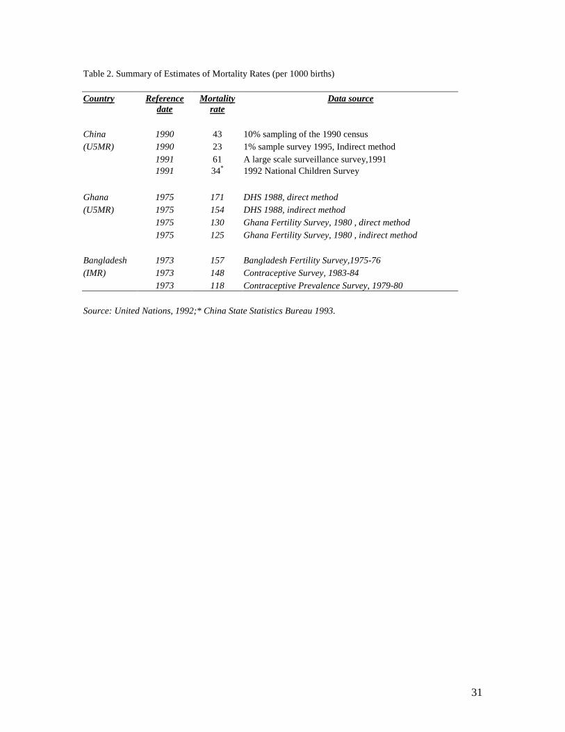
estimation methods.8 Table 2 summarizes the scale of discrepancy in mortality rates for

selective countries. The figures illustrate clearly the degree of sensitivity of mortality rate

estimates. For example, using two different data sources, under-5 mortality rate for

China in 1991 ranges from 34 to 61 per 1000 births. Hence, the credibility of the

empirical results, in particular based on cross-country data on health outcomes, depends

crucially on the availability of a database with health indicators estimated using common

methodology and comparable data sources such as DHS.

The DHS uses identical survey instruments across countries and estimates mortality rates

using a consistent method9. The DHS are nationally representative, hence a wide range

of basic population indicators (in addition to mortality rates) can also be constructed from

this data source. These indicators include basic household socio-economic characteristics,

fertility information, child nutrition status, and household access to services (safe water,

sanitation, and electricity), utilization of basic health and education services, mother’s

education and knowledge of treatment of common childhood illnesses. These basic

indicators are derived by applying expansion factors, so they are estimates of population

indicators for each country. The comprehensive coverage of the basic population

indicators provides us with a good opportunity to relate population health outcomes to

possible key determinants. Recently, Macro International has published all basic

7 There are principally two methods used to estimate mortality rates , namely direct and indirect methods. The former use complete maternal history information, while the latter is based on incomplete maternal history and implemented by imposing several assumptions, including (1) homogeneity of mortality risks by age group of mother, (2) stable fertility patterns, and (3) children being exposed to the same mortality risks, regardless of the mother’s age (United Nations, 1992). 8 In the database handbook for developing countries produced by the UN (1992), discrepancies between the direct and indirect estimates of child mortality rates are observed for many countries. 9 Since these surveys collect complete maternity history, child mortality rates can be estimated based on complete maternal history for all women in the DHS.

8

indicators for 60 countries between 1985 and 1999, both at the national level and for

urban and rural areas separately.

To estimate child mortality rates, in addition to demographic surveys, two other primary

data sources can also be used: (1) vital registration system data, and (2) census data. In

general, the vital registration system is not a reliable data source for developing countries

as the magnitude of incomplete registrations can be substantial, thus resulting in

significant measurement errors in the mortality rates (UN, 1992). Thanks to the recent

efforts from international organizations and national statistics offices in many developing

countries, a large number of countries are now able to conduct censuses periodically

(every 5 to 10 years), which provide an important data source for estimating mortality

rates at the national as well as regional level for a given country.10 But censuses are

limited in their coverage on socio-economic variables and, therefore, it is not always

possible to use censuses to address such issue as determination of health outcomes.

In contrast, DHS is an improved data source. But the sample size in DHS is relatively

small for conducting regional level (within a country) analysis on health. Empirical

studies focusing on explaining regional variations in health outcomes can often be more

informative in guiding county-specific policy design, while results from cross-country

analysis are generally useful for formulating global strategies. Given there are limitations

in all data sources as outlined above, one possible solution is to combine censuses with

DHS for conducting regional analysis on health outcomes. Recent work by Hentschel,

Lanjouw, Lanjouw and Poggi (2000), and Elbers, Lanjouw and Lanjouw (2000) has

developed a methodology of combining censuses with household surveys for poverty

analysis, and the empirical evidence of their studies have demonstrated encouragingly

that it is possible to apply the developed methodology to areas beyond poverty analysis,

e.g. to include health and environment issues.

10 Only a third of low-income countries have had a census since 1985 and 27 per cent of LDCs have a latest census that was conducted prior to 1975. As a result, infant mortality for many developing countries before 1990 are based on interpolations and extrapolations, and therefore, are not measurements (Deaton, 1995; Chamie, 1994).

9

3.2 Variable Definitions

Despite the many advantages of the DHS over other data sources, one of its limitations is

the absence of income or expenditure variable, which are generally regarded as good

measures of welfare. Filmer and Prichett (1998) propose the use of a wealth index as a

measure of welfare.11 They also illustrate that the ranking of households by their

economic positions based on the asset index are very close to that based on expenditure

(Filmer and Scott, 2001; Filmer and Pritchett, 2001). However, in this study, the key

objective is to select alternative policy interventions based on estimation of a health

outcome model. To this end, an income variable is more easy to interpret than a wealth

index, when comparing with other policy variables such as improvement in access to safe

water or sanitation, or female education. To overcome the problem of lack of income data

in DHS, we supplement the DHS data using WDI data which provides a country-level

time series of economic and social indicators, including GDP per capita and public

expenditure on health. To ensure consistency, we attempt to use variables derived from

the DHS to the extent possible and only resort to other sources when key variables are not

available from the survey.

Table 3 summaries all variables from DHS and WDI used in the estimation of the

mortality determination model. However, several variables, which are either constructed

specifically or chosen for specific reasons, deserve a separate discussion.

IMR and U5MR The mortality rates are estimated using a five-year period analysis

approach. By this method, IMR and U5MR are estimated using maternal history several

years preceding the survey year (e.g. 0-4, 5-10 or 11-15 years preceding the survey date).

We use the most recent estimates of mortality rates, i.e. 0-4 years preceding the survey

date. There are two advantages in using the estimates nearest to the survey year (0-4

years). First, the mortality rates can be regarded as a measure of average health outcomes

for the period between the survey date and five years prior to the survey. Secondly, the

11 Using principle component analysis, a wealth index can be derived by combining information from housing characteristics and possession of household durable goods.

10

measurement errors in mortality rates due to misreporting can be reduced, to some extent,

when using the more recent maternal history data.12

GDP per capita We use real GDP per capita at constant prices in the estimation and

match this income variable to corresponding child mortality rates constructed from the

DHS. GDP variables from the WDI are purchasing-power-parity adjusted and expressed

in current international dollars. To control for inflation (as the dates of DHS vary across

countries), we then convert all incomes into constant prices using the US CPI as the

deflator (1995 US CPI=100). In order to investigate the effects of both current and lagged

incomes on health, we construct several sets of GDP per capita variables: (1) five-year

moving average (MA) corresponding to the survey year, and (2) its lags.13

Share of health expenditure in GDP The information on the share of health expenditure is

only available periodically for most countries from the WDI. Therefore, including health

expenditure in the model can lead to a sharp reduction in sample size for the estimation.

To minimize the loss of observations, we therefore use a five-year average of health

expenditure shares for countries for which no corresponding health expenditure data at

the survey date is available. Such construction is reasonable as public expenditure tend to

move with GDP, and consequently, the shares of government expenditures remain

relatively stable over time.

Per capita health expenditure Information on per capita health expenditure from the

WDI is available for most DHS countries from 1990 to 1998. We construct a three-year

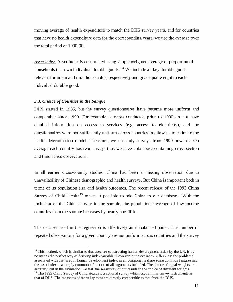
12 Our estimation of mortality rates for China shows clear evidence of downwards bias in IMR using retrospective questionnaires as respondents are more likely to treat the incidence of child death as never born, the longer the duration between the survey and time of the incidence. Using the 1992 China Children Survey, the estimated IMR for rural and urban areas between 1987-1992 are as follows:

Rural Urban Total 1987-88 21.1 13.9 19.6 1989-90 22.1 13.5 20.3 1991-92 32.1 13.7 28.1 The increasing trend of IMR in rural China is inconsistent with estimates from all other sources which show a consistent fall of IMR in rural areas over time. 13 To illustrate the procedure with an example by assuming the DHS survey year is 1995. There are two steps: (1) convert all GDP per capita into constant international $ using US CPI (CPI1995=100); and (2) construct moving average GDP90-95 using GDP per capita between 1990-95, and its lags (MA GDP85-90) using GDP per capita between 1985-90.

11

moving average of health expenditure to match the DHS survey years, and for countries

that have no health expenditure data for the corresponding years, we use the average over

the total period of 1990-98.

Asset index Asset index is constructed using simple weighted average of proportion of

households that own individual durable goods. 14 We include all key durable goods

relevant for urban and rural households, respectively and give equal weight to each

individual durable good.

3.3. Choice of Counties in the Sample

DHS started in 1985, but the survey questionnaires have became more uniform and

comparable since 1990. For example, surveys conducted prior to 1990 do not have

detailed information on access to services (e.g. access to electricity), and the

questionnaires were not sufficiently uniform across countries to allow us to estimate the

health determination model. Therefore, we use only surveys from 1990 onwards. On

average each country has two surveys thus we have a database containing cross-section

and time-series observations.

In all earlier cross-country studies, China had been a missing observation due to

unavailability of Chinese demographic and health surveys. But China is important both in

terms of its population size and health outcomes. The recent release of the 1992 China

Survey of Child Health15 makes it possible to add China to our database. With the

inclusion of the China survey in the sample, the population coverage of low-income

countries from the sample increases by nearly one fifth.

The data set used in the regression is effectively an unbalanced panel. The number of

repeated observations for a given country are not uniform across countries and the survey

14 This method, which is similar to that used for constructing human development index by the UN, is by no means the perfect way of deriving index variable. However, our asset index suffers less the problems associated with that used in human development index as all components share some common features and the asset index is a simply monotonic function of all arguments included. The choice of equal weights are arbitrary, but in the estimation, we test the sensitivity of our results to the choice of different weights. 15 The 1992 China Survey of Child Health is a national survey which uses similar survey instruments as that of DHS. The estimates of mortality rates are directly comparable to that from the DHS.

12

years vary by country. Given these constraints, we pool all surveys together. However,

the pooling of all observations implicitly assumes that the health outcomes are

independently distributed across countries and over time. The latter is hard to defend

given that many variables at the country level tend to be auto-correlated over time. In the

estimation, we relax this assumption and allow observations within each country to be

correlated16.

4. Estimation

To empirically estimate the health determination model, we need to address issues related

to the model specification. We begin with a model specification for health determination

by considering health outcomes as a function of key groups of variables (similar to that

in Filmer and Prichett, 1999). Our choice of explanatory variables are based both on

economic theory and empirical evidence from earlier work in this area. These include:

(1) incomes; (2) various social and environmental indicators, including the level of

female education, access to sanitation, and access to safe water; (3) policy variables such

as the share of public health expenditure in GDP or immunization coverage; and (4)

country-specific effects, e.g. the level of urbanization, the quality of government and

cultural effects. Such a grouping has an advantage with respect to our intended cost-

effectiveness analysis, as we can compare various alternative interventions, e.g.

improving access to female education versus improving access to sanitation when cost

data are available. A more detailed discussion on this is deterred to section 6.

The basic relationship can be summarized as follows:

Mortality Rates it = α*Income it + ββββ*Social Indicators it + ηηηη* Policy Instruments it

+ δδδδ*Country Specific Effects i + ε it

where ε it is the error term, following an identical and independent distribution.

We focus our discussion on three aspects of the model specification. These include: (1)

the possible two-way causation between health outcomes and included explanatory

variables such as income or government health expenditure; (2) the third variable effect,

16 We use an estimation method which allows cluster effects.

13

i.e. unobservable variables that may affect both income and health outcomes, e.g. quality

of government; and (3) the existence of heteroscedasticity and the effect of outliers.

These concerns related to model specification, to some extent, can be dealt with by

employing different estimation methods when data requirements can be met. For

example, use of an Instrumental Variable estimator (IV) can deal with issue (1) if we are

able to find valid instruments17, Fixed Effect estimation can solve the problems

associated with issue (2) if we have repeated observations for each country, and a

Weighted Least Square (WLS) estimator can help reduce the effects of outliers as

discussed in (3). In the following, we discuss these three aspects of the model

specification outlined above in the context of the estimation methodology.

4.1 Two-way causation

It is often argued that the robust positive correlation between health and income observed

in either cross-country or household-level data can be interpreted in two ways. As put by

Pritchett and Summers (1996): “wealthier is healthier” or “healthier is wealthier”? At the

international level, the evidence of a causal relationship between incomes and health is

inconclusive. To establish the causation, Pritchett and Summers (1996) have carried out a

thorough and extensive econometric analysis using a range of valid instrumental

variables that could be found and they conclude that there exists strong evidence in favor

of a causal and structural relationship running from income to health outcomes. Using a

similar approach, Filmer and Pritchett (1999) find no evidence supporting the two-way

causation between health outcomes and public health spending based on DHS data. These

studies have direct implications for our choice of estimation methods. In empirical

analysis, finding valid instrumental variables can be a formidable task on the one hand,

and on the other hand, any benefits derived from using IV can often be offset by its weak

inference power as the estimates of the standard errors from IV are usually much larger

than that from OLS.

17 Valid instrumental variables are those that are highly correlated with the explanatory variables concerned but not directly related to the health outcomes.

14

In reality, the impact of income on health is not instantaneous. It takes time for the

income effect to be fully transmitted into health outcomes, in particular at the national

level. Therefore, it makes sense to relate lagged incomes to current health outcomes.18 In

the following analysis, we use five-year moving averages of GDP per capita (five years

preceding the DHS survey year for each country) and relate it to the mortality rates

estimated from the corresponding DHS. Such a specification, to some extent, can avoid

the problem of two-way causality if it indeed exists. In light of the above empirical

evidence from the earlier studies and econometric considerations, we start our

specification assuming the causation running from incomes and public health expenditure

to health outcomes.

4.2 Third variable effect

Country-specific effects, such as the capacity of government to manage and deliver

health services, can affect both incomes and health outcomes simultaneously. However,

these third variables are not always observable or quantifiable. If the third variable is

country specific and time invariant, consistent estimates of the health model can be

obtained using either first-differencing or fixed-effect estimation. However, given that

only 28 countries in our sample have repeated observations, the sample size limitation

implies that the proposed estimation methods can not be empirically implemented. To

partially deal with this issue, we include in our model the share of rural population for

each country to act as a proxy variable for country-specific effects.

4.3 Heterogeneity and Outliers

It is highly possible that the sample estimates of IMR and U5MR may have a different

variance across countries and over time. The existence of heteroscadasticity in the error

terms, however, does not pose a serious problem in terms of obtaining consistent

estimates, as it only causes a bias in the estimates of standard errors, which can be

corrected using robust-t statistic estimates. But it is important to control for the effect of

outliers which can significantly bias estimates. In the following estimation, we assess the

influence of outliers in two ways. First, we estimate health models using both OLS and

18 Using DHS data, Hill and King (1992) find strong effects of lagged female enrollment on infant mortality.

15

WLS methods to check the consistency of the estimates. Secondly, we estimate the above

model by sequentially deleting one country each time to examine the robustness of

estimates to the exclusion of individual countries.

The ultimate objective of our empirical analysis is to identify all principle health

determinants and apply the estimated coefficients to an effectiveness analysis. Naturally,

we should start our model specification by including all “legitimate” exogenous

determinants of health outcomes. However, in the empirical analysis, we need to consider

the problem of multicollinearity due to the nature of cross-county data, which typically

has small sample size and high correlations among the explanatory variables. This

implies that we need to be selective in the choice of explanatory variables in order to

minimize the bias caused by omitted variable specifications. In the regression analysis,

we experiment with different model specifications to check the robustness of the results.

5. Results

We first investigate the simple bivariate association between mortality rates and all

potential explanatory variables. The correlation matrices are summarized in Appendix

Table 2a-2c. At the national level, variables which are highly correlated with mortality

rates, ranked in descending order, include access to electricity, asset index, GDP per

capita, access to piped water, access to sanitation, and female secondary education.

However, the ranking is different at the disaggregate level. In the urban data, mortality is

highly correlated to access to electricity, asset index and female secondary education,

while in rural areas, access to piped water, access to electricity, female education, asset

index and vaccination coverage are closely related with mortality. The rankings are

nearly identical for IMR and U5MR, which is not surprising given the high correlation

among the two indicators (over 0.92). To estimate the net impact of individual variables

on mortality, we use a multivariate regression approach to control for the possible

correlation among the explanatory variables. In the following, we estimate the health

determination model of IMR and U5MR using data both at the national level and

disaggregated by urban/rural sector.

16

Results for IMR

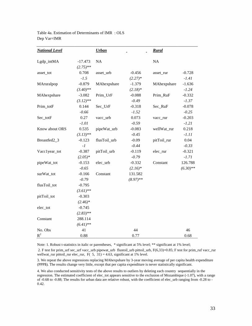
Table 4a summarizes the regression results for IMR. At the national level, the regression

results identify several factors that have a significant and robust impact on mortality, after

controlling for all other variables. These include incomes, share of health expenditure to

GDP, access to sanitation (flush or pit toilets), access to electricity, and vaccination

coverage in the first year of life. The aggregate data fit the model well with about 88% of

the variation in IMR being explained by the included variables. But, variables such as

female education and access to safe water, that were often found to play an important role

in determining IMR in earlier empirical studies, are not statistically significant in our

results.

The focus of this study is to go beyond the national level by conducting analysis also for

urban and rural areas separately. However, two key health determinants are not available

in the disaggregated data for rural and urban areas (1) incomes and (2) public health

expenditure. To obtain rural/urban incomes for each country we need to use other

household survey such as Living Standard Measurement Survey (LSMS) data to match

with the DHS data. However, this task can be particularly difficult to accomplish as it

requires converting rural and urban incomes into a comparable base using a rural/urban

price index, which is available only for few countries. In light of this data limitation, we

chose to include in the model a proxy variable for income, the asset index which

summarizes durable goods ownership. From the DHS data, the proportion of households

that own different consumer durable goods (TV, refrigerators, radio, bikes, motorbike

among others) can be estimated for urban and rural areas separately. We then construct

the asset index by a simple weighted average of key durable goods.19

Regarding health expenditure variable, we include the share of health expenditure of

GDP at the national level in the urban and rural regressions. This leads to a change in the

interpretation of the health variable. We effectively examine how rural and urban health

outcomes are affected as average health expenditure shares change.

19 We check the sensitivity of our estimates to different sets of weights, and find little changes in the results with respect to different weights. The following formula are used to construct the asset index:

asset_urb= 0.2*tv_urb + 0.2*frig_urb +0.2*radio_urb +0.2*bike_urb+0.2*mot_urb asset_rur= 0.2*tv_rur + 0.2*frig_rur +0.2*radio_rur +0.2*bike_rur+0.2*mot_rur

17

The regression results at the disaggregate level (Table 4a) differ significantly from that

generated using the aggregate level data. In urban areas, we find that access to electricity,

in particular, has a large impact on IMR, although asset index, and health expenditure

share are also statistically significant. But, other key health determinants such as female

education, access to safe water, access to sanitation, and vaccination coverage have no

significant effect on IMR, either individually, or jointly (the joint significance test,

F(6,33)=0.85).

In the rural result, none of the included variables is statistically significant, except that

access to electricity is significant only at the 10% level. The joint significant test on

female education, access to safe water, access to sanitation, and vaccination coverage

show that these variables jointly have a significant effect on reducing IMR in rural areas

(F(5,31)=4.63, significant at 1%). It is also interesting to observe that that increasing the

average share of health expenditure of GDP, reduces IMR in urban areas, but not in the

rural areas (although it has the right sign).

The results from the disaggregated data on IMR are unexpected. There might be two

possible explanations. First, the results could be a true reflection of reality. Given the fact

that a large body of medical evidence shows that most infant deaths occur in the first

month of birth, it may well be true that interventions in antenatal care might be the only

relevant factor explaining IMR and therefore, the included variables are expected play

little significant role in explaining IMR. However, only a few countries with DHS have

collected information on access to antenatal cares, therefore, the inclusion of this variable

in the estimation greatly reduces our sample size.20 To include access to antenatal care in

the model, we find a significant impact of antenatal care on IMR in urban areas

(coefficient -0.31; t(2.2)), but no effect in rural areas, nor at the national level.

The second explanation for the unexpected IMR results is a statistical one. The pattern of

the results at the disaggregate level, is quite striking – the models have very high

18

explanatory power, with R2 being 0.77 and 0.68 for urban and rural areas respectively,

yet with few significant estimates. To some extent, this suggests the existence of strong

multicollinearity, which is a typical feature of cross-county data. One of the major

limitations in the cross-country analysis lies in the difficulty of empirically estimating the

independent effect of key variables, mainly due to relatively small sample size. Given the

problems of high correlation among these variables, in the first stage of the analysis we

carry out extensive experiments to check the robustness of the results with respect to

choice of explanatory variables. We find that although the estimated coefficients are quite

sensitive to the inclusion of a few highly correlated variables,21 they remain relatively

stable to the variables listed in Table 3.

Results for U5MR

The estimation results for U5MR are reported in Table 4b. At the national level, income,

health expenditure share of GDP, access to electricity, vaccination coverage in the first

year of life, access to sanitation (pit toilet latrine) each has a significant impact on

reducing U5MR. To a large extent, the results for U5MR are similar to that for IMR,

except that most of the estimated coefficients are much larger in the U5MR model. For

example, the impact of access to electricity on U5MR is almost three times that of IMR

(the coefficient being –1.02 for U5MR, and –0.33 for IMR for urban data; -0.97 for

U5MR and –0.32 for IMR, for rural data), indicating that health interventions focusing on

improving household access to electricity could be a very effective policy for reducing

U5MR, but not necessarily so for IMR.

In urban areas, we find that access to electricity is the only important determinant of

U5MR, controlling for all other variables. But asset index, health expenditures, female

education, access to piped water, flush toilets, and pit toilets latrine jointly affect U5MR

(joint significance test, F(8,32)=2.20, significant at the 10% level). In rural areas,

however, vaccination coverage is an important factor which reduces child mortality

20 Note the inclusion of the antenatal care reduces the sample size from 48 to 22 for urban data, 46 to 28 for rural data, and 41 to 26 for the aggregate data, hence these results are not directly comparable with those reported in Table 4a. 21 When including both male and female education, or all types of access to water and sanitation, the regression results are very unstable.

19

(access to electricity is significant at the 10% level). It is interesting to observe that

increasing the share of health expenditure of GDP at the national level significantly

reduces the U5MR in rural areas, but not in the urban areas, while the opposite is

observed for IMR.

We should emphasize two issues related to the public health expenditure variable

included in the above estimation. First, how we can best measure public health

expenditure, i.e. choosing between the share of health expenditure of GDP and per capita

health expenditure (expressed in PPP$). Secondly, some of the included health

determinants (vaccination coverage and mother’s knowledge of ORS) could be regarded

as the outcomes of public health expenditure, therefore, estimation problems arise when

treating them as covariates in the model specification. To deal with the first issue, we

repeat all estimations replacing health expenditure shares by per capita health

expenditure. We find hardly any differences in the two sets of estimation results, except

that per capita health expenditure is never statistically significant. So we choose the share

of health expenditure in the final results. To test if some of the included variables are

outcomes of the public health expenditure, we compare estimation results from models

with and without including the health expenditure variable. The results show that health

expenditure and other included variables have independent impacts on health, i.e. all

estimates of RHVs are very robust to the exclusion of health expenditure variable. This

suggests the second issue related to the health expenditure variable is of little concern.

We also test the robustness of the results to outlier effects. This is done in two ways (1)

using the Weighted Least Square estimator22 and (2) performing regression analysis with

deleting one country in the sample sequentially. The WLS results (not reported) for IMR

are very close to that using the OLS, while the estimated coefficients for U5MR change

marginally depending on the choice of weighting variables.23

22 The weighting variables using GDP per capita, square root of population size, and their inverses. 23 The effect of breastfeeding seems to be less robust to the choice of estimation methods and weighting variables. When using GDP or the inverse of population as weights, breastfeeding variable becomes significant, but it is insignificant with the inverse of GDP or Population as the weighting variables.

20

The regression results from deleting one country sequentially in the sample appear

relatively stable. The range of the estimated coefficients are reported in the note of Table

4a–4b. The following discussion focuses only on those “interesting” coefficients, i.e. that

are significant and have the right sign. The estimated effect of access to electricity on

U5MR in urban areas changes from -1.15 (dropping Namibia) to -0.86 (dropping

Zambia). The coefficient of vaccination coverage in the rural data varies from -0.86

(dropping Brazil) to -0.52 (dropping Nicaragua). With regard to IMR, the estimated

coefficient of access to electricity in urban areas ranges from -0.28 to -0.42. The above

results suggest that the issues of heterogeneity and the effect of outliers are of secondary

concerns which, to a great extent, enhances our confidence in the findings based on OLS

method.

Access to Electricity

The finding that access to electricity has the largest impact in reducing mortality in

comparison to all other included variables (access to sanitation or safe water) is

particularly interesting. This finding is new as none of the earlier studies have identified

the electricity effect, partially due to data limitations. But why can connecting households

to electricity produce important health outcomes among low-income countries? One

possibility might be that, in the case of the urban and rural results, we do not have the

income variable and our constructed asset index may not have captured the income effect

fully, thus having access to electricity is, in fact, a proxy for incomes. Therefore, it may

be picking up the income effect.

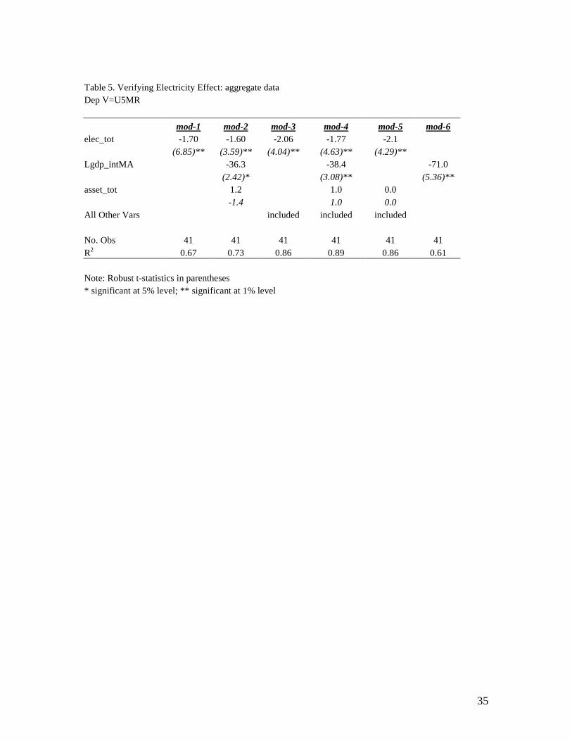
To empirically separate the electricity effect from income, we use data at the national

level where we have all three variables concerned: income, asset index, and access to

electricity. We check the effect of incomes and/or other variables on the coefficient of

the electricity variable using six different model specifications. Table 5 summarizes our

results for verifying the electricity effect.. We find that the estimated coefficient of access

to electricity is hardly affected by adding the income variable, after controlling for only

the asset index (mod-1 vs. mod-2) or controlling for all other relevant variables (mod-3

21

vs. mod-4)24. This indicates that access to electricity is likely to be independent of

incomes. Not only has the access to electricity an independent effect on mortality, it is

also a key underlying factor explaining mortality. This variable alone accounts for about

64% of variations in U5MR (mod-1), surpassing the income variable (mod-6) which

explains 67%, while all included variables account for 89% of the variation in U5MR.25

The coefficient for the asset variable is not significant with or without introducing

incomes in the specification (mod-4, and mod-5).

The above evidence indicates that access to electricity indeed has a significant and

independent (of income) impact on mortality. It is possible that households linked to

electricity may be more likely to use electric appliances (such as refrigerators,

microwaves, or kettles) or have access to hot water. These in turn can facilitate household

hygiene practices, hence reducing the possibility of contracting infectious diseases, in

particular among young children. Given the immediate implications of such findings for

operations and policy design, further research, in particular using regional-level or

household-level data for individual countries, is needed to verify the effect on mortality

of linking households to electricity.

In light of the new findings on the important electricity effect on mortality, it is useful to

revisit the income impact on health, which has been the strong emphasis in earlier

studies. Our results suggest that the income effect on health may have been grossly

overestimated in early cross countries studies, due to model misspecification that omits

access to electricity.26 This conjecture is borne out by the comparison of the two

specifications (mod-6 and mod-2) as shown in Table 6. We find that, when not

controlling for all other variables, the estimated gross income effect is large (-71), but this

coefficient is nearly halved (36.3), once introducing the electricity and asset variables to

the model.

24 The asset index and access to electricity has a correlation of 0.92, while asset index and income, and access to electricity and income have the same level of correlation with, being 0.80 and 0.93, respectively. 25 In the urban results, asset index is significant, but access to electricity is robust to the inclusion of asset index, but not vice versa. The electricity variable alone explains about 77% variation in U5MR, while all included variables explain 85% of total variation. 26 Almost all earlier empirical studies in this area, relate health indicators to income, a range of social indicators, and access sanitation and water, but never access to electricity.

22

There exists plenty of empirical evidence indicating that other factors besides incomes

are more important health determinants.27 For example, Anand and Ravallion (1993) find

the commonly observed health and income correlation vanishes once one controls for the

incidence of poverty and public spending on health. Hence, they argue that empirical

analysis on health issues should shift the focus towards factors beyond incomes in order

to provide useful information for designing more effective and relevant policies. Our

results provide additional support to this argument. Overall, empirical evidence seems to

show consistently, that it is possible to identify a range of low-cost health interventions

that are more effective in reducing mortality than polices which narrowly focus on

increasing national incomes.

6. Effectiveness Analysis

In principle we can apply the estimated coefficients from the model of health

determination to a cost-effectiveness analysis. The estimated coefficients provide

measures of the net impact of each intervention (which corresponds to each explanatory

variable), keeping all other impacts constant. In turn, the inverse of the estimates, which

we label as the effectiveness coefficients, are particularly useful for comparing various

alternative interventions. They provide a measure of what is required for each respective

intervention in order to achieve an outcome of a unit reduction in mortality, after

controlling for the effects of all other interventions. If we have relevant county-level

information (such as household population, number of female of schooling age and etc)

and the cost data on various projects designed for improving health outcomes including

access to safe water and sanitation, it is possible to perform a cost-effectiveness analysis

for the selection of different interventions. This is done by comparing the cost of each

alternative intervention that produces the same outcome (e.g. an unit reduction of child

27 Factors which are identified as important determinants of child mortality include mothers’ education and women’s status (Summers 1992, Caldwell 1986), effective public programs (Dreze and Sen, 1991) and income distribution (Deaton 2001). Using cross-region data on India, recent empirical evidence shows that the income effect can be slow and weak, and that other personal and social characteristics, such as female literacy often have more powerful influence on demographic outcomes including mortality (Murthi and Dreze, 1995).

23

mortality rate). The cost is calculated based on the cost of a project and the estimated

effectiveness coefficients.

In reality, however, care should be taken in the implementation of the above approach.

One of the main reasons is that it is not always possible to estimate precisely the net

effect of individual variables due to multicollinearity and sample size limitation as

illustrated in the above econometric results.

The underlying assumptions of our model specifications imply that the impact of each

intervention has an uniform impact on mortality reduction regardless of the level of

mortality. However, empirical evidence often suggests diminishing returns to

interventions, i.e. interventions can have a much bigger impact on reducing mortality, the

higher the mortality level. This suggests that a nonlinear functional form might better

capture the impact on mortality of various policies. In the effectiveness analysis, we

present results using both linear and nonlinear specifications28. As shown in Table 6, the

estimated effectiveness coefficients from the nonlinear model are broadly in line with that

from the linear model, except for income (with GDP growth rate being doubled in the

nonlinear model) and access to sanitation.

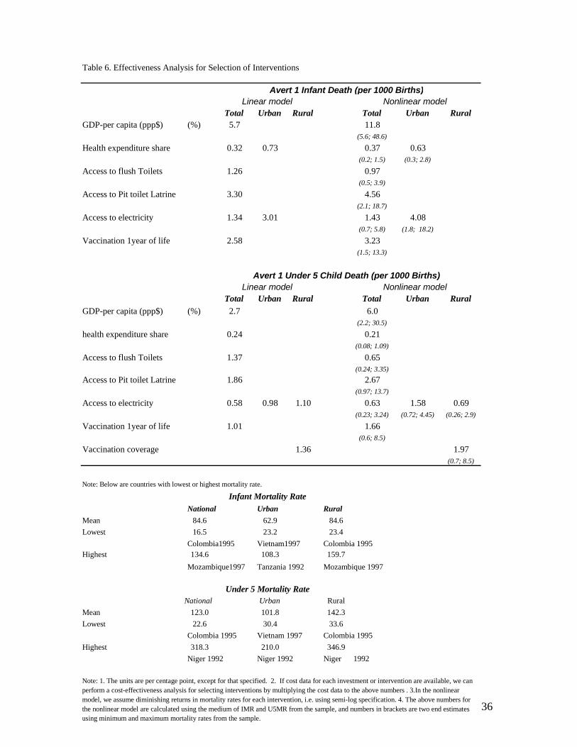
Table 6 summarizes the estimated cost-effectiveness coefficients for various

interventions to avert one infant and one child death per 1000 births. In the following

discussion we focus only on statistically significant estimates from the nonlinear model.

At the national level, to avert one under-five child death per 1000 births, there exist five

possible alternative investments (expressed in percentage point based on non-linear

function): (1) to increase household access to flush toilets by 0.7; (2) increase access to

pit toilet latrine by 2.7; (3) access to electricity by 0.6; (4) increase vaccination coverage

in first year of life by 1.7; or (5) increase share of health expenditure of GDP by 0.2. In

addition, macroeconomic policies which can produce an annual growth rate of per capita

28 We chose semi-log function so that the rate of mortality reduction of any intervention depends on the level of mortality and the cost-effectiveness coefficients. The numbers for the nonlinear model are calculated at the sample median, taking into account the fact that means are more sensitive to outliers than median.

24

GDP, of about 6 per cent, can also achieve the same outcomes of mortality reduction. The

interpretation of the health impact of GDP growth assumes growth does not cause

worsening of income distribution, or no linkages between income inequality and health

outcomes.

The numbers in the brackets summarize the two end point estimates of the effectiveness

coefficients for countries with the highest and lowest mortality rates. For example, Niger

(1992) has the highest U5MR (318 per 1000 births), and Colombia (1995) has the lowest

(23 per 1000 births). To reduce one under-5 child death per 1000 births, household access

to electricity needs to be increased by 0.2 percentage points for Niger, and 3 percentage

points for Colombia. The results clearly illustrate the point that it is much easier to reduce

mortality by choosing direct policy interventions such as improving access to electricity,

or expanding vaccination coverage than focusing on economic polices that aim to deliver

an annual per capita GDP about 6%, in particular, given the fact that the annual per capita

GDP among LDCs in the 1990s is less than 1% (WDI).

However, it should be emphasized that figures presented in Table 6 should be viewed as

an illustration of the methodology, and not be taken too literally for policy purposes. The

main reason is rooted in the limitations in cross-country data, as revealed in the

econometrics results presented in the above section, in providing robust empirical

evidence for policy design. Cross-county studies have their usefulness in capturing broad

patterns and trends in health outcomes at the global level, which is needed for

formulating overall policy strategies. However, to produce robust empirical evidence for

the purpose of designing policies, we should no doubt move beyond the cross-country

analysis, and conduct empirical studies using the sub-national level or household-level

data whenever possible.

7. Conclusion

The findings from the above cross-country analysis on health determination both

consolidate results from earlier studies and add new evidence in this area. First, our

results show that the disaggregate level analysis is more insightful than that focusing only

on the national average. Secondly, factors that significantly affect child mortality rates

25

differ between urban and rural areas. In urban areas, linking households to electricity has

been singled out as one of the key factors reducing both IMR and U5MR. Using the

national level data, we are able to show that the electricity effect on mortality is large,

significant and independent of incomes. In rural areas, we find that expanding

vaccination coverage significantly reduces U5MR. In general, the estimated impacts are

much bigger for U5MR than for IMR. Thirdly, the above econometrics results indicate

that despite our efforts in ensuring data comparability by constructing variables using

comparable DHS, cross-county data in general have limitations in providing robust

empirical results. Variables at the country level are often highly correlated, which makes

it difficulty to disentangle individual impacts on mortality. This suggests that we should

be cautious in deriving policy implications from empirical results based on cross-county

data sources. In order to have a bearing on policy recommendations, future studies should

focus on explaining regional variations in health outcomes based on sub-national data or

household level analysis on health determination to supplement cross-country analysis.

26

References Anand, S and M Ravallion, (1993), “Human Development in Poor Countries: On the Role of Private Incomes and Public Services’, Journal of Economic Perspectives, Vol 7, No 1, pp133-150. Claeson, M, E Bos, T Mawji & I Pathmanathan (2000), Reducing Child Mortality in India in the new Millennium, Bulletin of the World Health Organization, 2000, 78 (1). China Statistics Bureau (1993), Proceedings on Survey and Research: 1992 national survey of the situation of children, China Statistics Bureau publishing house. Deaton, A and C Paxson, (1999). “Mortality, Education, Income, and Inequality among American Cohorts”. Working Paper No. 7140. Cambridge, MA: National Bureau of Economic Research. Deaton, A, (2001), “Relative Deprivation, Inequality, and Mortality”. Working Paper No, 8099. Cambridge, MA: National Bureau of Economic Research. Deaton, A, (1999), “Inequalities in Income and Inequalities in Health”. Working Paper 7141. Cambridge, MA: National Bureau of Economic Research. Dreze, J and M Murthi (1999), “Fertility, Education and Development: Further Evidence from India”, Population and Development Review, 27 Filmer, D and L Pritchett, (1999), “The impact of public spending on health: does money matter?” Social Science and Medicine No. 49, pp 1309-1323. Filmer, D and L Pritchett (2001), “Estimating Wealth Effects without Expenditure Data-or Tears: An Application to Educational Enrollments in States of India”. Demography 38 (1) Filmer, D, E. M. King and L Pritchett, (1998), “Gender Disparity in South Asia: Comparisons Between and Within Countries.” Policy Research Working Paper 1867, The World Bank. Flegg, T. A., (1982), “Inequality of Income, Illiteracy and Medical Care as Determinants of Infant Mortality in Underdeveloped Countries”, Population Studies, Vol. 36, Issue 3, pp 441-458. Gwatkin, D, (2000), “Health Inequalities and the Health of the Poor: What Do We Know? What Can We Do?”, Bulletin of the World Health Organization, 2000, 78 (1) Gwatkin, D., S. Rutstein, K. Johnson, R. Pande, and A. Wagstaff, Socioeconomic Differences in Health, Nutrition and Population. 2000, The World Bank: Washington DC.

27

Hentschel, J, J. O. Lanjouw, P Lanjouw and J Poggi, (2000), “Combining Census and Survey Data to Trace the Spatial Dimensions of Poverty: A Case Study of Ecuador”. The World Bank Economic Review, Vol. 14, No. 1, pp 147-65. Hill, K and D. M. Upchurch, (1995), “Gender Differences in Child Health: Evidence from the Demographic and Health Surveys”. Population and Development Review, Vol. 21, Issue 1, pp 127-151. Hughes, G, K Lvovsky and M Dunleavy, (2001), “Environmental Health in India: Priorities in Andhra Pradesh”, Environment and Social Development Unit, South Asia Region, The World Bank. Jalan, J and M Ravallion, (2000), “Does Piped Water Improve Child Health in Poor Families? Propensity Score Matching Estimates for Rural India”. Policy research working paper, The World Bank . Kahn, R, P. Wise, B Kennedy and I Kawachi (2000), “State income inequality, household income, and maternal mental and physical health: cross sectional national survey”. British Medical Journal, Kaplan, A., George, Elsie R. Pamuk, J. W. Lynch, Richard D. Cohen and Jennifer L. Balfour (1996), “Inequality in income and mortality in the United States: analysis of mortality and potential pathways”. British Medical Journal, 312, 999-1003 Kawachi, I and B. P. Kennedy (1997), “Socioeconomic determinants of health : Health and social cohesion: why care about income inequality?” Kennedy, P.B. , I Kawachi and D Prothrow-Smith (1996), “Income distribution and mortality: cross sectional ecological study of the Robin Hood index in the United States”. British Medical Journal 314:1194-1037. Marmot, M and M Bobak, (2000), “International comparators and poverty and health in Europe”. British Medical Journal, 321:1124-1128. Murthi, M, Guio A, and J Dreze (1995), “Mortality, Fertility and Gender Bias in India: A District Level Analysis”, Population and Development Review, 9. Pritchett, L. and L. H. Summers (1996), “Wealthier is Healthier”, Journal of Human Resources, XXXI 4, pp841-868. Rutstein S, (2000), “Factors Associated with Trends in Infant and Child Mortality in Developing Countries during the 1990s”, Bulletin of the World health Organization, 2000, 78 (10) Shi, A (2000), “How Access to Urban Potable Water and Sewerage Connections Affect Child Mortality”, Policy research working paper 2274, The World Bank.

28

Srinivasan, T.N., (1994), “Data base for development analysis: An overview,” Journal of Development Economics 44 pp.3-27. United Nations, 1992. Child Mortality since the 1960s : A data base for developing countries. United Nations, New York. Wagstaff, A (2000), “Socioeconomic Inequalities in Child Mortality: Comparisons Across Nine Developing Countries”, Bulletin of the World Health Organization, 2000, 78 (1) Wagstaff, A. (2000), “Unpacking the Causes of Inequalities in Child Survival: The Case of Cebu, The Philippines”. Policy Research working paper, The World Bank. Wagstaff, A. (2001), “Poverty and Health”, Paper presented to the World Health Organization Commission on Macroeconomics and Health. Wagstaff, A. (2001), “Inequalities in Health in Developing Countries: Swimming Against the Tide?”, Policy research working paper 2795, the World Bank.

29

IMR: Level and Inequality

-0.3

-0.25

-0.2

-0.15

-0.1

-0.05

00 20 40 60 80 100 120 140 160

Level of IMR (per 1000 births)

Con

cent

ratio

n In

dex

correlation=-0.33

U5MR: Level and Inequality

-0.3

-0.25

-0.2

-0.15

-0.1

-0.05

00 50 100 150 200 250 300 350

Level of U5MR (per 1000 births)

Con

cent

ratio

n In

dex

correlation=-0.59

30

Table 1. Urban/Rural Gaps in Mortality Rate: Levels and Decline Rates by Region Region Country Year IMR U5MR

Rural Urban Rural Urban Africa Cameroon 1991 86 72 159 120 1998 87 61 160 111 Niger 1992 143 89 347 210 1998 147 80 327 178 Asia Philippines 1993 44 32 73 53 1998 40 31 63 46 Indonesia 1991 81 57 117 84 1997 58 36 79 48 Bangladesh 1994 103 81 153 114 1997 91 73 131 96 S. America Brazil 1991 107 81 127 95

1996 65 42 79 49 Colombia 1990 23 29 34 36 1995 35.2 28.3 43.2 34.1

Global Level All DHS countries Early 1990s 87 67 143 105 End 1990s 77 58 126 89

Decline Rate (%, per annum)

1.7 2.1 2.1 2.6

Source: The mortality rates are from the DHS website. The decline rates are estimated by the author.

31

Table 2. Summary of Estimates of Mortality Rates (per 1000 births) Country Reference

date Mortality

rate Data source

China 1990 43 10% sampling of the 1990 census (U5MR) 1990 23 1% sample survey 1995, Indirect method 1991 61 A large scale surveillance survey,1991

1991 34* 1992 National Children Survey

Ghana 1975 171 DHS 1988, direct method (U5MR) 1975 154 DHS 1988, indirect method 1975 130 Ghana Fertility Survey, 1980 , direct method 1975 125 Ghana Fertility Survey, 1980 , indirect method Bangladesh 1973 157 Bangladesh Fertility Survey,1975-76 (IMR) 1973 148 Contraceptive Survey, 1983-84 1973 118 Contraceptive Prevalence Survey, 1979-80 Source: United Nations, 1992;* China State Statistics Bureau 1993.

32

Table 3. Summary of Key Variables Variable Definition Mean S.Dev 1q0_total Infant mortality rate, national level (per 1000 births) 72 28

1q0_Urban Urban households (per 1000 births) 63 22

1q0_Rural Rural households (per 1000 births) 85 31 5q0_total Under-five mortality rate, national level (per 1000 births) 119 65 5q0_Urban Urban households (per 1000 births) 100 49 5q0_Rural Rural households (per 1000 births) 140 69 MA GDPpc Five-year moving average of GDP per capita (ppp$, at 1995 price), (log), from

WDI 7 1

MAruralpop Five-year moving average of share of rural population (%), from WDI. 61 19 MAhexpshare Share of health expenditure to GDP (%), from WDI. This variable is replaced by a

five-year moving average of the share of health expenditure for countries that do not have health expenditure data matching the mortality data at survey year.

5 2

MAHexp_pca Three-year moving average of per capita health expenditure (ppp $), from WDI. For countries where no health expenditure data is available for the corresponding DHS, we replace the observations by the average of health expenditure between 1990-1998.

105 107

prim_totf Percent of household population with female age 6 and over having primary education (%)

40 16

sec_totf Percent of household population with female age 6 and over having secondary education (%)

18 16

breastfed2_3 Proportion of children who were breastfed for 2-3 months, (%) 23 22 pipewat_tot proportion of households having access to piped water, national level, (%) 43 23 wellwat_tot proportion of household having access to well water, national level, (%) 31 21 surwat_tot proportion of households having access to surface water, national level, (%) 20 17 flustoil_tot proportion of households having access to flush toilets, national level, (%) 23 24 pittoil_tot proportion of households having access to pit toilets latrine, national level, (%) 44 27 elec_tot proportion of households linked to electricity, national level, (%) 40 32 vacc_tot Percentage of children who had received all vaccines by the time of the

survey,national level, (%) 52 19

vacc1year_tot proportion of children vaccinated in the first year of life, national level, (%) 36 18 Assindex_urb Index for possession of durable goods for urban households, (%) 32 19

Assindex_rur Index for possession of durable goods for rural households, (%) 22 14 Assindex_tot Index for possession of durable goods for all households, (%) 25 15 knowORS_tot proportion of women who have knowledge about oral rehydration, national level,

(%) 74 20

Antenatal care Proportion of live births from women who have visited health professionals during pregnancy, National level, (%)

38 32

33

Table 4a. Estimation of Determinants of IMR : OLS Dep Var=IMR National Level Urban Rural Lgdp_intMA -17.473 NA NA (2.75)** asset_tot 0.708 asset_urb -0.456 asset_rur -0.728 -1.5 (2.27)* -1.41 MAruralpop -0.879 MAhexpshare -1.379 MAhexpshare -1.636 (3.40)** (2.18)* -1.24 MAhexpshare -3.082 Prim_UrF -0.088 Prim_RuF -0.332 (3.12)** -0.49 -1.37 Prim_totF 0.144 Sec_UrF -0.318 Sec_RuF -0.078 -0.66 -1.52 -0.25 Sec_totF 0.27 vacc_urb 0.073 vacc_rur -0.203 -1.01 -0.59 -1.21 Know about ORS 0.535 pipeWat_urb -0.083 wellWat_rur 0.218 (3.13)** -0.45 -1.11 Breastfed2_3 -0.123 flusToil_urb -0.09 pitToil_rur 0.04 -1 -0.44 -0.33 Vacc1year_tot -0.387 pitToil_urb -0.119 elec_rur -0.321 (2.05)* -0.79 -1.71 pipeWat_tot -0.153 elec_urb -0.332 Constant 126.788 -0.65 (2.16)* (6.30)** surWat_tot -0.166 Constant 131.582 -0.79 (8.97)** flusToil_tot -0.795 (3.61)** pitToil_tot -0.303 (2.46)* elec_tot -0.745 (2.83)** Constant 288.114 (6.41)** No. Obs 41 44 46 R2 0.88 0.77 0.68

Note: 1. Robust t-statistics in italic or parentheses, * significant at 5% level; ** significant at 1% level; 2. F test for prim_urf sec_urf vacc_urb pipewat_urb flustoil_urb pittoil_urb, F(6,33)=0.85; F test for prim_ruf vacc_rur wellwat_rur pittoil_rur elec_rur, F( 5, 31) = 4.63, significant at 1% level. 3. We repeat the above regressions replacing MAhexpshare by 3-year moving average of per capita health expenditure (PPP$). The results change very little, except that per capita expenditure is never statistically significant.

4. We also conducted sensitivity tests of the above results to outliers by deleting each country sequentially in the regression. The estimated coefficient of elec_tot appears sensitive to the exclusion of Mozambique (-1.07), with a range of -0.68 to -0.88; The results for urban data are relative robust, with the coefficient of elec_urb ranging from -0.28 to -0.42.

34

Table 4b. Estimation of Determinants of U5MR : OLS Dep Var = U5MR National level Urban Rural Lgdp_intMA -37.333 NA NA (2.93)** asset_tot 0.333 asset_urb -0.755 asset_rur -1.279 -0.29 -2.01 -0.86 MAruralpop -1.58 MAhexpshare -1.31 MAhexpshare -4.229 (3.44)** -1.06 (2.62)* MAhexpshare -4.192 Prim_UrF -0.508 Prim_RuF -0.616 -1.98 -1.3 -1.35 Prim_totF 0.054 Sec_UrF -0.47 Sec_RuF 0.283 -0.15 -1.37 -0.39 Sec_totF 0.931 vacc_urb 0.043 vacc_rur -0.739 -1.66 -0.25 (2.05)* Know about ORS 0.422 pipeWat_urb -0.267 pipeWat_rur 0.152 -1.18 -1.06 -0.2 Breastfed2_3 -0.236 flusToil_urb -0.449 wellWat_rur 0.849 -1.19 -1.12 -1.42 Vacc1year_tot -0.99 pitToil_urb -0.47 pitToil_rur 0.026 (2.22)* -1.31 -0.13 pipeWat_tot -0.523 elec_urb -1.023 elec_rur -0.969 -1.06 (3.75)** -1.71 surWat_tot -0.875 Constant 295.983 Constant 224.309 -1.52 (9.25)** (5.56)** flusToil_tot -0.732 -1.44 pitToil_tot -0.535 -1.96 elec_tot -1.713 (4.17)** Constant 643.503 (5.53)** No. Obs 41 44 46 R2 0.89 0.85 0.8 Note: 1. Robust t-statistics in Italic or parentheses, * significant at 5% level; ** significant at 1% level; 2.F test for asset_urb MAhexp prim_urf sec_urf vacc_urb pipewat_urb flustoil_urb pittoil_urb, F(8, 32) = 2.20, significant at 10%; F test for asset_rur MAhexpshare prim_ruf vacc_rur wellwat_rur pittoil_rur elec_rur, F(7, 30) =5.81, significant at 5%. 3. We repeat the above regression replacing MA health expenditure share by MA per capita health expenditure (PPP$). The results remain very close to above, except that per capita expenditure is never statistically significant.

4.The sensitivity tests show that results at the national level are relatively robust, with the coefficient of ele_tot ranging from -1.39 (dropping Senegal) to -1.92 (dropping Dominican Republic); Vacc1year_tot ranging -1.25 (Peru) to -0.73 (Zambia); coefficient of PitToil_tot ranging from -0.83 (Zambia) to -0.48 (Namibia). The estimated coefficient for elec_urb changes from -1.145 (dropping Namibia) to -0.86 (dropping Zambia). For the rural data, the coefficient of vacc-rur ranges from -0.86 (dropping Brazil) to -0.52 (dropping Nicaragua); and the coefficient of elec_rur ranges from -1.23 (dropping Jordan) to -0.48 (dropping Philippines).

35

Table 5. Verifying Electricity Effect: aggregate data Dep V=U5MR mod-1 mod-2 mod-3 mod-4 mod-5 mod-6 elec_tot -1.70 -1.60 -2.06 -1.77 -2.1 (6.85)** (3.59)** (4.04)** (4.63)** (4.29)** Lgdp_intMA -36.3 -38.4 -71.0 (2.42)* (3.08)** (5.36)** asset_tot 1.2 1.0 0.0 -1.4 1.0 0.0 All Other Vars included included included No. Obs 41 41 41 41 41 41 R2 0.67 0.73 0.86 0.89 0.86 0.61 Note: Robust t-statistics in parentheses * significant at 5% level; ** significant at 1% level

36

Table 6. Effectiveness Analysis for Selection of Interventions

Total Urban Rural Total Urban RuralGDP-per capita (ppp$) (%) 5.7 11.8

(5.6; 48.6)

Health expenditure share 0.32 0.73 0.37 0.63(0.2; 1.5) (0.3; 2.8)

Access to flush Toilets 1.26 0.97(0.5; 3.9)

Access to Pit toilet Latrine 3.30 4.56(2.1; 18.7)

Access to electricity 1.34 3.01 1.43 4.08(0.7; 5.8) (1.8; 18.2)

Vaccination 1year of life 2.58 3.23(1.5; 13.3)

Total Urban Rural Total Urban RuralGDP-per capita (ppp$) (%) 2.7 6.0

(2.2; 30.5)

health expenditure share 0.24 0.21(0.08; 1.09)

Access to flush Toilets 1.37 0.65(0.24; 3.35)

Access to Pit toilet Latrine 1.86 2.67(0.97; 13.7)

Access to electricity 0.58 0.98 1.10 0.63 1.58 0.69(0.23; 3.24) (0.72; 4.45) (0.26; 2.9)

Vaccination 1year of life 1.01 1.66(0.6; 8.5)

Vaccination coverage 1.36 1.97(0.7; 8.5)

Note: Below are countries with lowest or highest mortality rate.

National Urban RuralMean 84.6 62.9 84.6Lowest 16.5 23.2 23.4

Colombia1995 Vietnam1997 Colombia 1995Highest 134.6 108.3 159.7

Mozambique1997 Tanzania 1992 Mozambique 1997

National Urban RuralMean 123.0 101.8 142.3Lowest 22.6 30.4 33.6

Colombia 1995 Vietnam 1997 Colombia 1995Highest 318.3 210.0 346.9

Niger 1992 Niger 1992 Niger 1992

Avert 1 Infant Death (per 1000 Births)Linear model Nonlinear model

Avert 1 Under 5 Child Death (per 1000 Births)

Under 5 Mortality Rate

Linear model Nonlinear model

Note: 1. The units are per centage point, except for that specified. 2. If cost data for each investment or intervention are available, we can perform a cost-effectiveness analysis for selecting interventions by multiplying the cost data to the above numbers . 3.In the nonlinear model, we assume diminishing returns in mortality rates for each intervention, i.e. using semi-log specification. 4. The above numbers for the nonlinear model are calculated using the medium of IMR and U5MR from the sample, and numbers in brackets are two end estimates using minimum and maximum mortality rates from the sample.

Infant Mortality Rate

37

Appendix Tables Table 1. DHS Countries and Survey Years by Region Sub-Saharan Africa Europe/Eurasia Asia Latin America & Caribbean Benin 1996 Mali 1987 Kazakhstan 1995 Bangladesh 1994 Bolivia 1994 Botswana 1988 Mali 1996 Kyrgyz Republic 1997 Bangladesh 1997 Bolivia 1998 Burkina Faso 1992 Morocco 1987 Turkey 1993 India 1993 Brazil 1986 Burkina Faso 1999 Morocco 1992 Turkey 1998 India 1999 Brazil 1991 Burundi 1987 Mozambique 1997 Uzbekistan 1996 Indonesia 1987 Brazil 1996 Cameroon 1991 Namibia 1992 Indonesia 1991 Colombia 1986 Cameroon 1998 Niger 1992 Indonesia 1994 Colombia 1990 CAR 1994 Niger 1998 Indonesia 1997 Colombia 1995 Chad 1997 Nigeria 1990 Nepal 1996 Dominican Republic 1986 Comoros 1996 Ondo State 1986 Pakistan 1991 Dominican Republic 1991 Cote d'Ivoire 1994 Rwanda 1992 Philippines 1993 Dominican Republic 1996 Egypt 1988 Senegal 1986 Philippines 1998 Ecuador 1987 Egypt 1992 Senegal 1993 Sri Lanka 1987 El Salvador 1985 Egypt 1995 Senegal 1997 Thailand 1987 Guatemala 1987 Eritrea 1995 Sudan 1990 Vietnam 1997 Guatemala 1995 Ghana 1988 Tanzania 1992 China 1992 Guatemala 1999 Ghana 1993 Tanzania 1996 Haiti 1994 Ghana 1998 Togo 1988 Mexico 1987 Guinea 1999 Togo 1998 Nicaragua 1997 Jordan 1990 Tunisia 1988 Paraguay 1990 Jordan 1997 Uganda 1988 Peru 1986 Kenya 1989 Uganda 1995 Peru 1992 Kenya 1993 Yemen 1991 Peru 1996 Kenya 1998 Yemen 1997 Trinidad & Tobago 1987 Liberia 1986 Zambia 1992 Madagascar 1992 Zambia 1996 Madagascar 1997 Zimbabwe 1988 Malawi 1992 Zimbabwe 1994

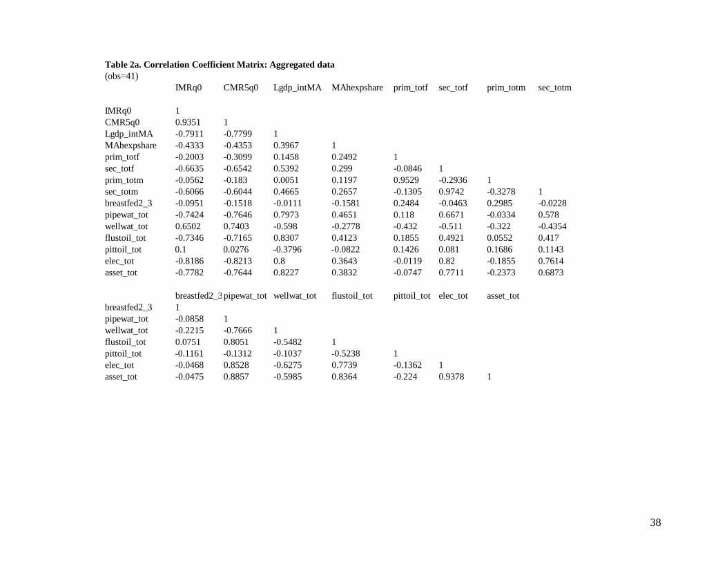
38

Table 2a. Correlation Coefficient Matrix: Aggregated data(obs=41)

IMRq0 CMR5q0 Lgdp_intMA MAhexpshare prim_totf sec_totf prim_totm sec_totm

IMRq0 1CMR5q0 0.9351 1Lgdp_intMA -0.7911 -0.7799 1MAhexpshare -0.4333 -0.4353 0.3967 1prim_totf -0.2003 -0.3099 0.1458 0.2492 1sec_totf -0.6635 -0.6542 0.5392 0.299 -0.0846 1prim_totm -0.0562 -0.183 0.0051 0.1197 0.9529 -0.2936 1sec_totm -0.6066 -0.6044 0.4665 0.2657 -0.1305 0.9742 -0.3278 1breastfed2_3 -0.0951 -0.1518 -0.0111 -0.1581 0.2484 -0.0463 0.2985 -0.0228pipewat_tot -0.7424 -0.7646 0.7973 0.4651 0.118 0.6671 -0.0334 0.578wellwat_tot 0.6502 0.7403 -0.598 -0.2778 -0.432 -0.511 -0.322 -0.4354flustoil_tot -0.7346 -0.7165 0.8307 0.4123 0.1855 0.4921 0.0552 0.417pittoil_tot 0.1 0.0276 -0.3796 -0.0822 0.1426 0.081 0.1686 0.1143elec_tot -0.8186 -0.8213 0.8 0.3643 -0.0119 0.82 -0.1855 0.7614asset_tot -0.7782 -0.7644 0.8227 0.3832 -0.0747 0.7711 -0.2373 0.6873

breastfed2_3pipewat_tot wellwat_tot flustoil_tot pittoil_tot elec_tot asset_totbreastfed2_3 1pipewat_tot -0.0858 1wellwat_tot -0.2215 -0.7666 1flustoil_tot 0.0751 0.8051 -0.5482 1pittoil_tot -0.1161 -0.1312 -0.1037 -0.5238 1elec_tot -0.0468 0.8528 -0.6275 0.7739 -0.1362 1asset_tot -0.0475 0.8857 -0.5985 0.8364 -0.224 0.9378 1

39

Table 2b. Correlation Coefficient Matrix: Urban data

(obs=43)

q01_urb q05_urb asset_urb prim_urf sec_urf elec_urb pipewat_urb surwat_rur flustoil_rur pittoil_rur vacc_urb MAhexpshare

q01_urb 1q05_urb 0.9185 1asset_urb -0.7592 -0.7845 1prim_urf 0.2538 0.1469 -0.4478 1sec_urf -0.7026 -0.6848 0.6682 -0.4389 1elec_urb -0.8055 -0.8787 0.8245 -0.2456 0.6642 1pipewat_urb -0.5521 -0.6234 0.5268 -0.0486 0.5118 0.5632 1surwat_rur 0.207 0.1363 -0.3906 0.4712 -0.0276 -0.1033 -0.1243 1flustoil_rur -0.5146 -0.5079 0.5146 0.0192 0.1987 0.46 0.2322 -0.2506 1pittoil_rur -0.185 -0.2656 0.0481 0.0361 0.3365 0.1344 0.1719 0.0864 -0.2804 1vacc_urb -0.0738 -0.1475 0.0009 0.2649 0.0278 0.0651 0.4888 0.0801 0.1757 -0.0029 1MAhexpshare -0.4239 -0.417 0.3059 0.0737 0.2945 0.3184 0.4593 -0.0883 0.1264 0.0657 0.2414 1

40

Table 2c. Correlation Coefficient Matrix: Rural data

(obs=44)

q01_rur q05_rur asset_rur MAruralpoMAhexpsvacc_rur pittoil_rur flustoil_rur surwat_rur pipewat_rur elec_rur sec_ruf prim_ruf

q01_rur 1q05_rur 0.9321 1asset_rur -0.6606 -0.6586 1MAruralpop 0.4316 0.5203 -0.4872 1MAhexpshare -0.3805 -0.413 0.1984 -0.3444 1vacc_rur -0.5408 -0.623 0.3387 -0.2723 0.4831 1pittoil_rur -0.2959 -0.3524 0.2463 0.0534 0.1131 0.3644 1flustoil_rur -0.5295 -0.4918 0.5018 -0.5667 0.1 0.3345 -0.2857 1surwat_rur 0.0933 -0.0026 -0.4217 0.0497 -0.0303 0.0966 0.1093 -0.2563 1pipewat_rur -0.6755 -0.6956 0.764 -0.5597 0.1765 0.3663 0.3104 0.4719 -0.3238 1elec_rur -0.667 -0.6834 0.9107 -0.4629 0.1202 0.2697 0.3021 0.4718 -0.3678 0.7827 1sec_ruf -0.5474 -0.5436 0.7626 -0.1874 0.0971 0.3035 0.4745 0.1096 -0.1708 0.5693 0.8187 1prim_ruf -0.4388 -0.5267 0.0399 -0.4143 0.4115 0.5604 0.1934 0.3517 0.4552 0.2492 0.071 -0.0064 1

41

42