determinants of stock market performance in...
TRANSCRIPT
B31
DETERMINANTS OF STOCK MARKET PERFORMANCE IN MALAYSIA
BY
KWONG SEN MIN
TAN HAW SHYAN
TAN HENG SIANG
TAN XIN YING
TUNG MUN YEE
A research project submitted in partial fulfilment of the requirement for the degree of
BACHELOR OF FINANCE (HONS)
UNIVERSITI TUNKU ABDUL RAHMAN
FACULTY OF BUSINESS AND FINANCE DEPARTMENT OF FINANCE
APRIL 2017

Determinants of Stock Market Performance in Malaysia
i
Copyright @ 2017
ALL RIGHTS RESERVED. No part of this paper may be reproduced, stored in a
retrieval system, or transmitted in any form or by any means, grap hic, electronic,
mechanical, photocopying, recording, scanning, or otherwise, without the prior
consent of the authors.
Determinants of Stock Market Performance in Malaysia
ii
DECLARATION
We hereby declare that:
(1) This undergraduate research project is the end result of our own work and that due
acknowledgement has been given in the references to ALL sources of information be
they printed, electronic, or personal.
(2) No portion of this research project has been submitted in support of any
application for any other degree or qualification of this or any other university, or
other institutes of learning.
(3) Equal contribution has been made by each group member in completing the
research project.
(4) The word count of this research report is 15391 words.
Name of Student:
Student ID: Signature:
1. KWONG SEN MIN
13ABB06066 .
2. TAN HAW SHYAN
13ABB02061 .
3. TAN HENG SIANG
14ABB04826 .
4. TAN XIN YING
13ABB05663 .
5. TUNG MUN YEE
14ABB04498 .
Date: 12th April 2017
Determinants of Stock Market Performance in Malaysia
iii
ACKNOWLEDGEMENT
We would like to express our deepest appreciation to all those who have provided the
assistance to complete this research. A special gratitude to our supervisor, Encik
Aminuddin Bin Ahmad for his contribution, suggestions and encouragement to
complete the research. We really appreciate his passion and input especially when we
are facing difficulties in completing our research. Encik Aminuddin really inspired us
to be more confidence when we were in doubt and loss of direction during the
progress. We are extremely thankful to him. We would also like to thank the second
examiner, Cik Hartini Binti Ab Aziz, for her suggestions to improve the project
Furthermore, we are thankful for the supports and facilities provided by Universiti
Tunku Abdul Rahman (UTAR). We are able to obtain the data required in a more
convenient provided in the library. Besides, we would like to acknowledge every
lecturers and tutors from UTAR who have provided us the knowledge in every
subjects, especially the subject of Econometric.
Finally, we would also like to express our sincere thanks to our friends and parents
for their wise counsel and a sympathetic ear. Thanks to everyone for supporting us
spiritually throughout the research project.
Determinants of Stock Market Performance in Malaysia
iv
TABLE OF CONTENT
Page
Copyright ................................................................................................................ i
Declaration ............................................................................................................. ii
Acknowledgement ................................................................................................. iii
Table of Content .............................................................................................. iv-viii
List of Tables ......................................................................................................... ix
List of Figures ......................................................................................................... x
List of Appendices ................................................................................................. xi
List of Abbreviations ....................................................................................... xii-xiv
Abstract ................................................................................................................. xv
CHAPTER 1: RESEARCH OVERVIEW
1.0 Introduction ....................................................................................................... 1
1.1 Research Background ....................................................................................... 1
1.1.1 Stock Market Crash in the History .................................................. 1-3
1.1.2 Stock Market in Malaysia ................................................................3-4
1.1.2.1 History of Stock Exchange in Malaysia ............................. 3
1.1.2.2 Volatility of Stock Market in Malaysia ........................... 4-6
1.2 Problem Statement ............................................................................. 6-8
1.3 Research Objectives .............................................................................. 8
1.3.1 General Objective ................................................................... 8
1.3.2 Specific Objectives ...............................................................8-9
1.4 Research Questions ............................................................................... 9
1.5 Hypotheses of the Study ........................................................................ 9
1.5.1 Exchange Rate .......................................................................10
1.5.2 Inflation Rate ........................................................................ 10
1.5.3 U.S. Stock Market Performance ........................................... 10
1.5.4 Crude Oil Price …………………….........…........................ 11
Determinants of Stock Market Performance in Malaysia
v
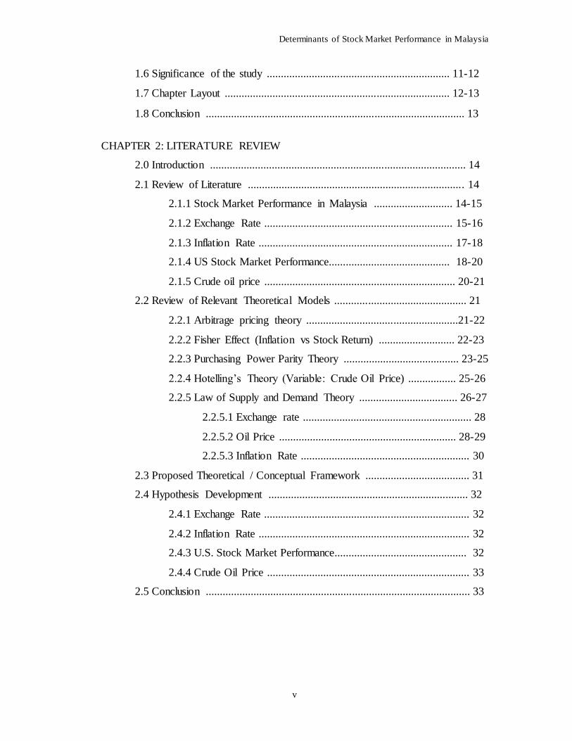
1.6 Significance of the study ................................................................. 11-12
1.7 Chapter Layout ................................................................................ 12-13
1.8 Conclusion ............................................................................................ 13
CHAPTER 2: LITERATURE REVIEW
2.0 Introduction ........................................................................................... 14
2.1 Review of Literature ............................................................................. 14
2.1.1 Stock Market Performance in Malaysia ............................ 14-15
2.1.2 Exchange Rate ................................................................... 15-16
2.1.3 Inflation Rate ..................................................................... 17-18
2.1.4 US Stock Market Performance........................................... 18-20
2.1.5 Crude oil price .................................................................... 20-21
2.2 Review of Relevant Theoretical Models ............................................... 21
2.2.1 Arbitrage pricing theory ......................................................21-22
2.2.2 Fisher Effect (Inflation vs Stock Return) ........................... 22-23
2.2.3 Purchasing Power Parity Theory ......................................... 23-25
2.2.4 Hotelling’s Theory (Variable: Crude Oil Price) ................. 25-26
2.2.5 Law of Supply and Demand Theory ................................... 26-27
2.2.5.1 Exchange rate ............................................................ 28
2.2.5.2 Oil Price ............................................................... 28-29
2.2.5.3 Inflation Rate ............................................................ 30
2.3 Proposed Theoretical / Conceptual Framework ..................................... 31
2.4 Hypothesis Development ....................................................................... 32
2.4.1 Exchange Rate ......................................................................... 32
2.4.2 Inflation Rate ........................................................................... 32
2.4.3 U.S. Stock Market Performance............................................... 32
2.4.4 Crude Oil Price ........................................................................ 33
2.5 Conclusion .............................................................................................. 33
Determinants of Stock Market Performance in Malaysia
vi
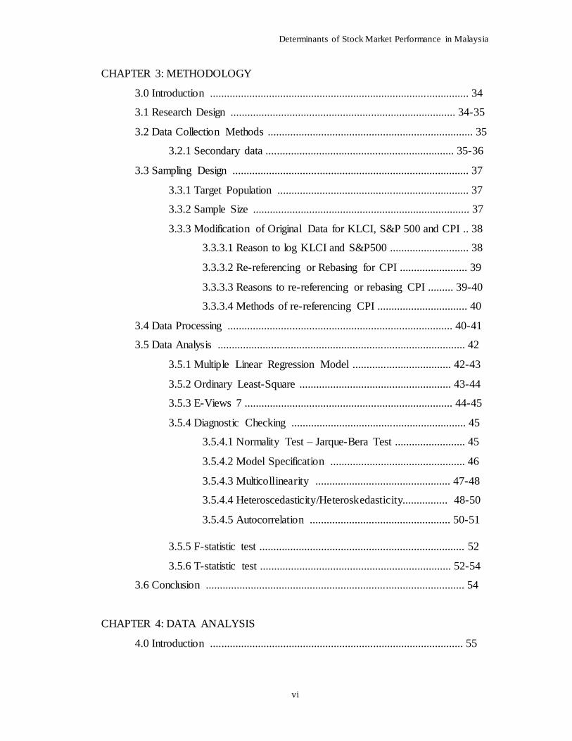
CHAPTER 3: METHODOLOGY
3.0 Introduction ............................................................................................ 34
3.1 Research Design ................................................................................ 34-35
3.2 Data Collection Methods ......................................................................... 35
3.2.1 Secondary data ................................................................... 35-36
3.3 Sampling Design .................................................................................... 37
3.3.1 Target Population .................................................................... 37
3.3.2 Sample Size ............................................................................. 37
3.3.3 Modification of Original Data for KLCI, S&P 500 and CPI .. 38
3.3.3.1 Reason to log KLCI and S&P500 ............................ 38
3.3.3.2 Re-referencing or Rebasing for CPI ........................ 39
3.3.3.3 Reasons to re-referencing or rebasing CPI ......... 39-40
3.3.3.4 Methods of re-referencing CPI ................................ 40
3.4 Data Processing ................................................................................ 40-41
3.5 Data Analysis ........................................................................................ 42
3.5.1 Multiple Linear Regression Model ................................... 42-43
3.5.2 Ordinary Least-Square ...................................................... 43-44
3.5.3 E-Views 7 .......................................................................... 44-45
3.5.4 Diagnostic Checking .............................................................. 45
3.5.4.1 Normality Test – Jarque-Bera Test ......................... 45
3.5.4.2 Model Specification ................................................ 46
3.5.4.3 Multicollinearity ................................................ 47-48
3.5.4.4 Heteroscedasticity/Heteroskedasticity................ 48-50
3.5.4.5 Autocorrelation .................................................. 50-51
3.5.5 F-statistic test ......................................................................... 52
3.5.6 T-statistic test .................................................................... 52-54
3.6 Conclusion ............................................................................................ 54
CHAPTER 4: DATA ANALYSIS
4.0 Introduction .......................................................................................... 55
Determinants of Stock Market Performance in Malaysia
vii
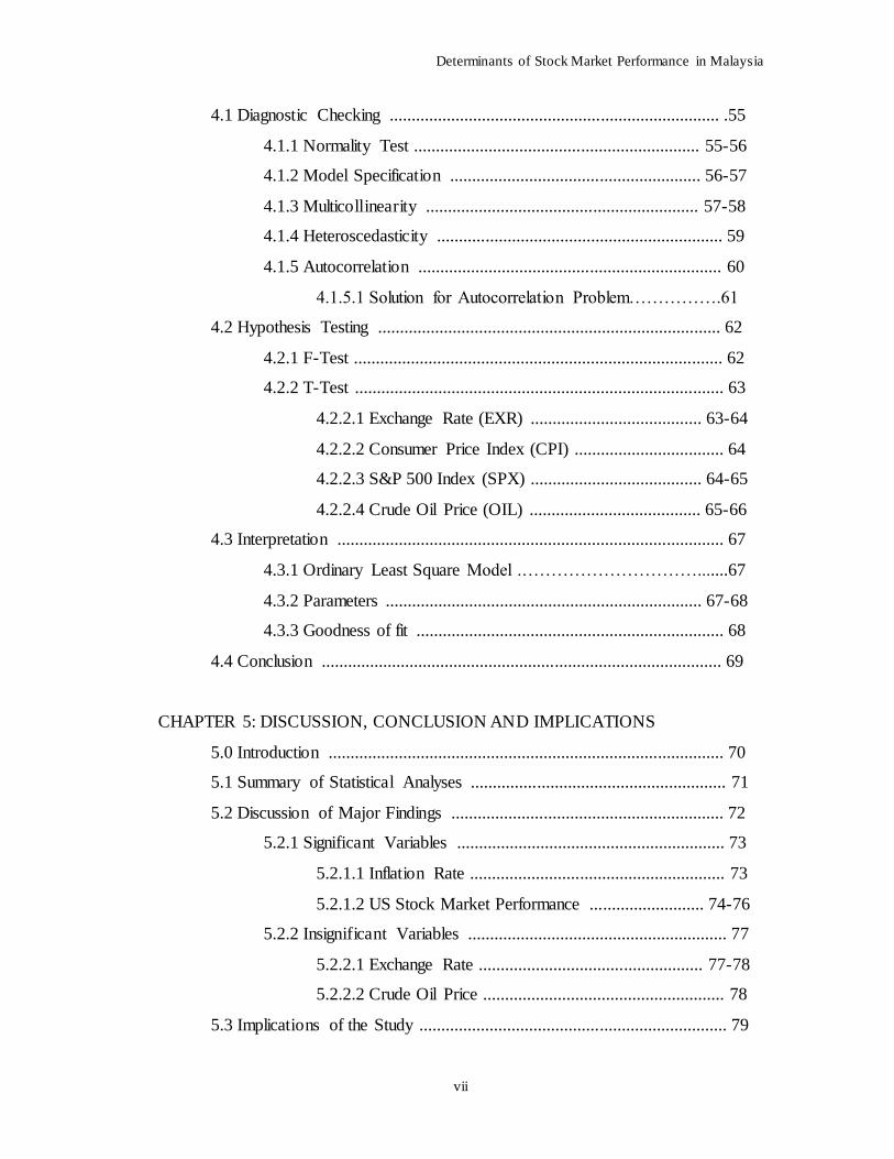
4.1 Diagnostic Checking ........................................................................... .55
4.1.1 Normality Test ................................................................. 55-56
4.1.2 Model Specification ......................................................... 56-57
4.1.3 Multicollinearity .............................................................. 57-58
4.1.4 Heteroscedasticity ................................................................. 59
4.1.5 Autocorrelation ..................................................................... 60
4.1.5.1 Solution for Autocorrelation Problem…………….61
4.2 Hypothesis Testing .............................................................................. 62
4.2.1 F-Test .................................................................................... 62
4.2.2 T-Test .................................................................................... 63
4.2.2.1 Exchange Rate (EXR) ....................................... 63-64
4.2.2.2 Consumer Price Index (CPI) .................................. 64
4.2.2.3 S&P 500 Index (SPX) ....................................... 64-65
4.2.2.4 Crude Oil Price (OIL) ....................................... 65-66
4.3 Interpretation ........................................................................................ 67
4.3.1 Ordinary Least Square Model .………………………….......67
4.3.2 Parameters ........................................................................ 67-68
4.3.3 Goodness of fit ...................................................................... 68
4.4 Conclusion ........................................................................................... 69
CHAPTER 5: DISCUSSION, CONCLUSION AND IMPLICATIONS
5.0 Introduction .......................................................................................... 70
5.1 Summary of Statistical Analyses .......................................................... 71
5.2 Discussion of Major Findings .............................................................. 72
5.2.1 Significant Variables ............................................................. 73
5.2.1.1 Inflation Rate .......................................................... 73
5.2.1.2 US Stock Market Performance .......................... 74-76
5.2.2 Insignificant Variables ........................................................... 77
5.2.2.1 Exchange Rate ................................................... 77-78
5.2.2.2 Crude Oil Price ....................................................... 78
5.3 Implications of the Study ...................................................................... 79
Determinants of Stock Market Performance in Malaysia
viii
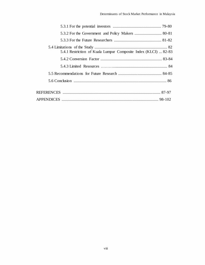
5.3.1 For the potential investors ................................................ 79-80
5.3.2 For the Government and Policy Makers ........................... 80-81
5.3.3 For the Future Researchers ............................................... 81-82
5.4 Limitations of the Study ........................................................................ 82 5.4.1 Restriction of Kuala Lumpur Composite Index (KLCI) ... 82-83
5.4.2 Conversion Factor ............................................................. 83-84
5.4.3 Limited Resources ………...................................................... 84
5.5 Recommendations for Future Research ........................................... 84-85
5.6 Conclusion ............................................................................................ 86
REFERENCES ................................................................................................. 87-97
APPENDICES ................................................................................................ 98-102
Determinants of Stock Market Performance in Malaysia
ix
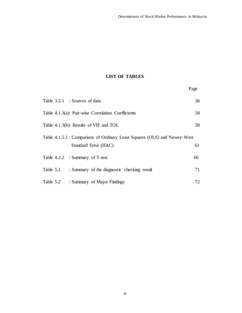
LIST OF TABLES
Page
Table 3.2.1 : Sources of data 36
Table 4.1.3(a): Pair-wise Correlation Coefficients 58
Table 4.1.3(b): Results of VIF and TOL 58
Table 4.1.5.1 : Comparison of Ordinary Least Squares (OLS) and Newey-West
Standard Error (HAC) 61
Table 4.2.2 : Summary of T-test 66
Table 5.1 : Summary of the diagnostic checking result 71
Table 5.2 : Summary of Major Findings 72
Determinants of Stock Market Performance in Malaysia
x
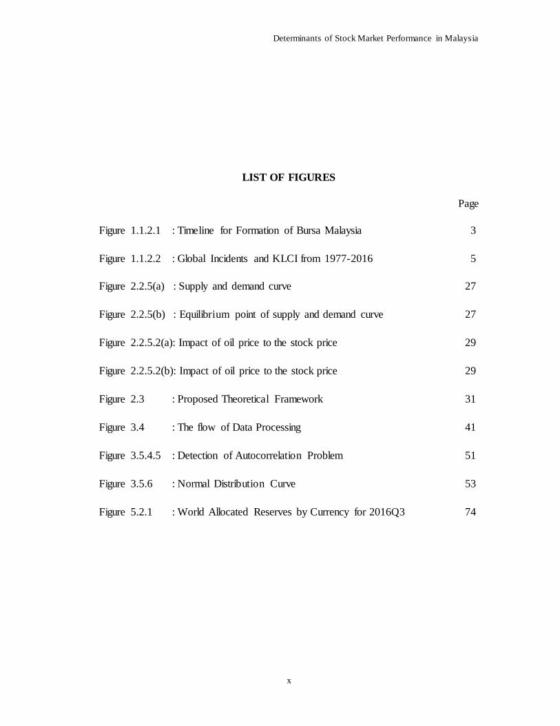
LIST OF FIGURES
Page
Figure 1.1.2.1 : Timeline for Formation of Bursa Malaysia 3
Figure 1.1.2.2 : Global Incidents and KLCI from 1977-2016 5
Figure 2.2.5(a) : Supply and demand curve 27
Figure 2.2.5(b) : Equilibrium point of supply and demand curve 27
Figure 2.2.5.2(a): Impact of oil price to the stock price 29
Figure 2.2.5.2(b): Impact of oil price to the stock price 29
Figure 2.3 : Proposed Theoretical Framework 31
Figure 3.4 : The flow of Data Processing 41
Figure 3.5.4.5 : Detection of Autocorrelation Problem 51
Figure 3.5.6 : Normal Distribution Curve 53
Figure 5.2.1 : World Allocated Reserves by Currency for 2016Q3 74
Determinants of Stock Market Performance in Malaysia
xi
LIST OF APPENDICES
Page
Appendix 1: Normality Test 101
Appendix 2: Autocorrelation Test 102
Appendix 3: Heteroscedasticity Test 103
Appendix 4: Model Specification Test 104
Appendix 5: OLS Regression Result (after correcting autocorrelation) 105
Determinants of Stock Market Performance in Malaysia
xii
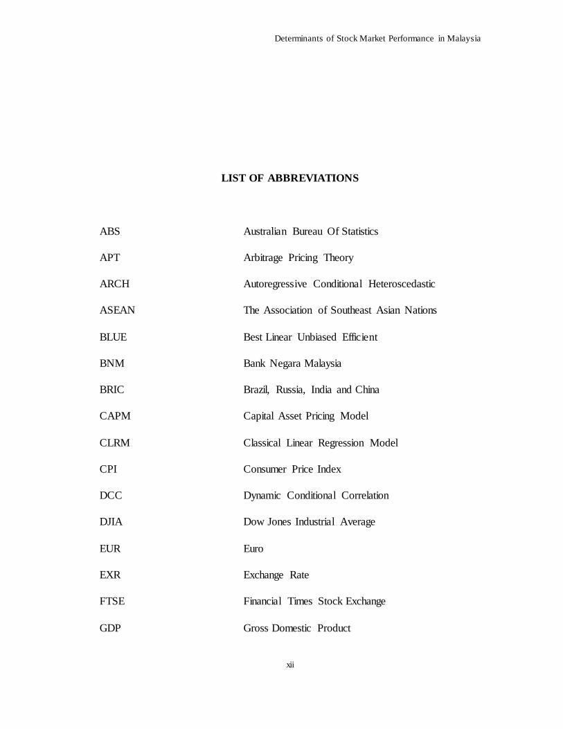
LIST OF ABBREVIATIONS
ABS Australian Bureau Of Statistics
APT Arbitrage Pricing Theory
ARCH Autoregressive Conditional Heteroscedastic
ASEAN The Association of Southeast Asian Nations
BLUE
BNM
BRIC
Best Linear Unbiased Efficient
Bank Negara Malaysia
Brazil, Russia, India and China
CAPM Capital Asset Pricing Model
CLRM Classical Linear Regression Model
CPI
DCC
Consumer Price Index
Dynamic Conditional Correlation
DJIA
EUR
Dow Jones Industrial Average
Euro
EXR Exchange Rate
FTSE Financial Times Stock Exchange
GDP Gross Domestic Product
Determinants of Stock Market Performance in Malaysia
xiii
HAC Heteroskedasticity And Autocorrelation Consistent
KLCI Kuala Lumpur Composite Index
KLSE Kuala Lumpur Stock Exchange
LOP Law of One Price
MSE Malayan Stock Exchange
OIL Crude Oil Price
OLS Ordinary Least Squares
PCA Principle Components Analysis
PLS Partial Squares Regression
PPP Purchasing Power Parity
RESET Ramsey’s Regression Specification Error Test
RM
SARS
Ringgit Malaysia
Severe Acute Respiratory Syndrome
S&P500 Standard & Poor’s 500 Index
SEM Stock Exchange Of Malaysia
SPX Standard & Poor’s 500 Index
TOL Tolerance
US
USD
United Sates
United States Dollar
VIF Variance Inflation Factor
WLS
WTI
Weighted Least Squares
West Texas Intermediate

Determinants of Stock Market Performance in Malaysia
xiv
WWI World War I
Determinants of Stock Market Performance in Malaysia
xv
Abstract
For years, the study of determinants for stock market performance are well-
documented. However, most of the studies are focus on the macroeconomic factors in
the developed country context. In light of this, this research intends to bright the gap
by examining the factors that affect the stock market performance in developing
country namely Malaysia. More specifically, this research aims to extend the current
literature reviews by including inflation rate, exchange rate, oil price and U.S. stock
market performance in determining their relationships with the Malaysian stock
market performance. By using Ordinary Least-Square regression method in E-views 7,
multiple linear regression analysis is performed to examine the hypotheses and
statistical relationships in a monthly basis from January 2009 to July 2016. The
results conclude that U.S. stock market performance and inflation rate have a positive
and negative relationship respectively with Malaysian stock market performance. On
the other hand, this research also indicates that both the exchange rate and oil price
have an insignificant relationship with Malaysian stock market performance.
Keywords: Malaysian stock market performance, multiple linear regression analysis,
inflation rate, exchange rate, oil price, U.S. stock market performance
Determinants of Stock Market Performance in Malaysia
Page 1 of 102
CHAPTER 1: RESEARCH OVERVIEW
1.0 Introduction
This chapter will give an overview of this research. Section 1.1 will discuss about the
research background and then follow by the problem statement in section 1.2. Section
1.3 and Section 1.4 will present the research objectives and research questions
respectively. In Section 1.5, hypotheses of the study will be formulated and continue
by explaining the significance of the study in section 1.7. Then, this chapter will end
with the chapter layout and conclusion.
1.1 Research Background
The study of stock market remains as one of the main interests for researches over the
past decades. This is because the stock market is not only important for the investors
who want to increase their wealth over times, but also important to the economy of a
country since the stock market can act as one of the leading indicators for a country’s
current and future economy condition. This paper, therefore, is designed to
investigate the factors affecting the stock market particularly in Malaysia.
1.1.1 Stock Market Crash in the History
Determinants of Stock Market Performance in Malaysia
Page 2 of 102
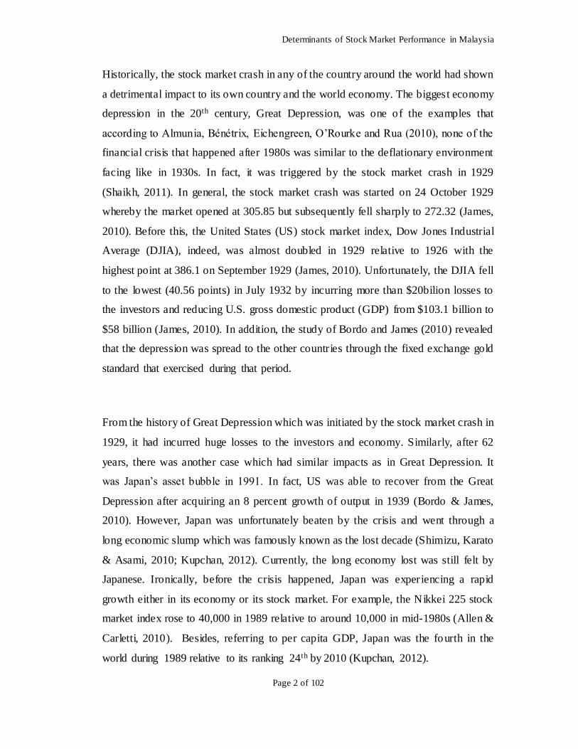
Historically, the stock market crash in any of the country around the world had shown
a detrimental impact to its own country and the world economy. The biggest economy
depression in the 20th century, Great Depression, was one of the examples that
according to Almunia, Bénétrix, Eichengreen, O’Rourke and Rua (2010), none of the
financial crisis that happened after 1980s was similar to the deflationary environment
facing like in 1930s. In fact, it was triggered by the stock market crash in 1929
(Shaikh, 2011). In general, the stock market crash was started on 24 October 1929
whereby the market opened at 305.85 but subsequently fell sharply to 272.32 (James,
2010). Before this, the United States (US) stock market index, Dow Jones Industrial
Average (DJIA), indeed, was almost doubled in 1929 relative to 1926 with the
highest point at 386.1 on September 1929 (James, 2010). Unfortunately, the DJIA fell
to the lowest (40.56 points) in July 1932 by incurring more than $20bilion losses to
the investors and reducing U.S. gross domestic product (GDP) from $103.1 billion to
$58 billion (James, 2010). In addition, the study of Bordo and James (2010) revealed
that the depression was spread to the other countries through the fixed exchange gold
standard that exercised during that period.
From the history of Great Depression which was initiated by the stock market crash in
1929, it had incurred huge losses to the investors and economy. Similarly, after 62
years, there was another case which had similar impacts as in Great Depression. It
was Japan’s asset bubble in 1991. In fact, US was able to recover from the Great
Depression after acquiring an 8 percent growth of output in 1939 (Bordo & James,
2010). However, Japan was unfortunately beaten by the crisis and went through a
long economic slump which was famously known as the lost decade (Shimizu, Karato
& Asami, 2010; Kupchan, 2012). Currently, the long economy lost was still felt by
Japanese. Ironically, before the crisis happened, Japan was experiencing a rapid
growth either in its economy or its stock market. For example, the Nikkei 225 stock
market index rose to 40,000 in 1989 relative to around 10,000 in mid-1980s (Allen &
Carletti, 2010). Besides, referring to per capita GDP, Japan was the fourth in the
world during 1989 relative to its ranking 24th by 2010 (Kupchan, 2012).
Determinants of Stock Market Performance in Malaysia
Page 3 of 102
However, when the enormous burble in stock prices and property prices were burst, a
large wealth that accumulated before this collapsed (Martin & Ventura, 2012). The
most direct impact from this asset bubble was the loss of 201 trillion yen and 36.4
trillion yen respectively in stock holdings from nonfinancial firms and banks between
1989 and 1991 (Kupchan, 2012). As a result, the whole country, either by firms or
citizens, were prudent in spending because of the pessimistic future expectation on
Japan’s economy.
1.1.2 Stock Market in Malaysia
1.1.2.1 History of Stock Exchange in Malaysia
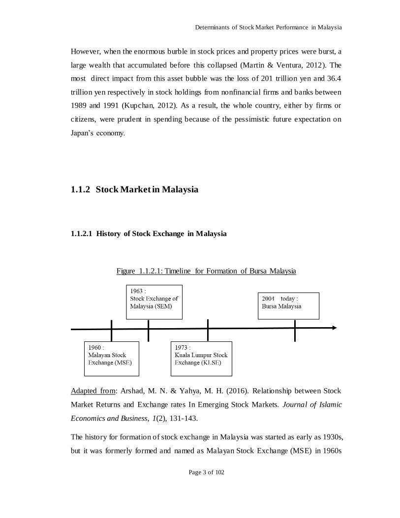
Figure 1.1.2.1: Timeline for Formation of Bursa Malaysia
Adapted from: Arshad, M. N. & Yahya, M. H. (2016). Relationship between Stock
Market Returns and Exchange rates In Emerging Stock Markets. Journal of Islamic
Economics and Business, 1(2), 131-143.
The history for formation of stock exchange in Malaysia was started as early as 1930s,
but it was formerly formed and named as Malayan Stock Exchange (MSE) in 1960s
Determinants of Stock Market Performance in Malaysia
Page 4 of 102
(Arshad & Yahya, 2016). After the formation of Malaysia in 1963, the stock
exchange was again changed its name to Stock Exchange of Malaysia (SEM). Indeed,
this stock exchange was the common trading floor for Malaysia and Singapore.
Besides, the currency for Malaysia and Singapore was exchangeable at par
(RM1=S$1) which was known as exchange rate interchangeability since they were
interdependent in terms of economy prior to 1973 (Schenk, 2013). However,
Malaysia was terminated the interchangeability in 1973. Subsequently, the Stock
Exchange of Singapore and Malaysia were separated at the same year. Under the new
change, Singapore stock exchange was named as Stock Exchange of Singapore
whereas Malaysia stock exchange was named as Kuala Lumpur Stock Exchange
(KLSE) (Ibrahim, 2006; Arshad & Yahya, 2016). However, KLSE was renamed as
Bursa Malaysia in 2004. After that, based on Arshad and Yahya (2016), Bursa
Malaysia had recorded a number of 1,145 listed companies with a combination of
around $235.28 billion in their market capitals at the end of February 2014.
1.1.2.2 Volatility of Stock Market in Malaysia
The globalization of market among the countries was an inevitable trend in the late of
20th century. In fact, Malaysia is benefited from this globalization era due to the
reduction of financial and trade barrier among countries. (Yeoh, Hooy and Arsad,
2010). By exporting resources such as tin, rubber and palm oil, Malaysia had
achieved a significant growth in economy from 1970s to 1990s. Besides, Malaysian
stock market was grown tremendously in view of the importance to attract foreign
capitals for the economy growth (Yeoh et al., 2010). However, the integration of
financial sector with the global market was not always beneficial to the country. This
view was supported by James (2010) and Tuyon and Ahmad (2016). They agreed that
the integration would lead to more volatility of the stock market.
Determinants of Stock Market Performance in Malaysia
Page 5 of 102
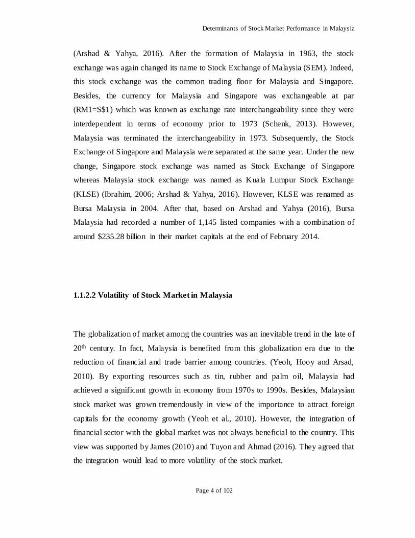
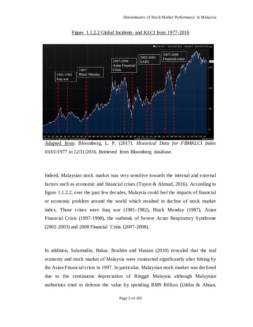
Figure 1.1.2.2 Global Incidents and KLCI from 1977-2016
Adapted from: Bloomberg, L. P. (2017). Historical Data for FBMKLCI Index
03/01/1977 to 12/31/2016. Retrieved from Bloomberg database.
Indeed, Malaysian stock market was very sensitive towards the internal and external
factors such as economic and financial crises (Tuyon & Ahmad, 2016). According to
figure 1.1.2.2, over the past few decades, Malaysia could feel the impacts of financial
or economic problem around the world which resulted in decline of stock market
index. Those crises were Iraq war (1981-1982), Black Monday (1987), Asian
Financial Crisis (1997-1998), the outbreak of Severe Acute Respiratory Syndrome
(2002-2003) and 2008 Financial Crisis (2007-2008).
In addition, Salamudin, Bakar, Ibrahim and Hassan (2010) revealed that the real
economy and stock market of Malaysia were contracted significantly after hitting by
the Asian Financial crisis in 1997. In particular, Malaysian stock market was declined
due to the continuous depreciation of Ringgit Malaysia although Malaysian
authorities tried to defense the value by spending RM9 Billion (Uddin & Ahsan,
Determinants of Stock Market Performance in Malaysia
Page 6 of 102
2014). Likewise, by looking to a more recent case which was 2008 Financial Crisis,
Malaysia was also inevitably affected by this global crisis. Indeed, the number of
companies listed in Bursa Malaysia and their market capitals were decreased after the
financial crises (Yeoh et al., 2010).
Through the history of stock crash and the volatility that experienced by Malaysian
stock market, it was clear that stock market would affect by either internal or external
factors.
1.2 Problem Statement
As mentioned above, the stock market is a vital part for a country’s economy.
Undeniably, it plays a crucial role to support the economy growth of a country. Hence,
many researchers have highlighted that the stock market of a country can work as an
indicator to measure the economic development of that country. Many policymakers
and investors believe that large decrease in stock index will lead to a future recession
while dramatically boost of stock index is a reflection of a future economy growth.
Recently, instability of Kuala Lumpur Composite Index (KLCI) has gained attentions
from researches. This study will examine the determinants of the Malaysian stock
market performance.
Indeed, investors invest their capitals in the stock market to protect themselves from
the high anticipated inflation. Both Kaur (2015) and Subramanian (2015) explained
that high inflation rate would significantly boost the stock market performance.
Besides, the exchange rate is one of the determinants of Malaysian stock market
performance as it might significantly affect the decision of the foreign investment in
Determinants of Stock Market Performance in Malaysia
Page 7 of 102
Malaysia. More specifically, Mutuku and Ng’eny (2015) claimed that exchange rate
is significantly related to the stock market performance in a positive manner.
On the other hand, US stands a significant position in the world economy. This might
be due to the US dollar is a key currency for international trades. Most of the central
bank and government in the world hold US dollar as their main international reserve
currency (Lee, 2013). In light of this, investors around the world are concerned about
any news that affecting US stock market. In fact, after the collapse of Lehman
Brothers in 2008, the global economy was critically hit by the financial shock.
Although KLCI is not as liquid as the foreign stock exchange market, decline of US
stock market still rampage in the Malaysian stock market. The history showed that the
KLCI was dropped from 1400 above to 850 below. This implies US Stock market
might give a significant impact to the performance of Malaysian stock market.
Besides, Hadi, Yahya and Shaari (2009) stated that Malaysia is an oil production and
exports country. As an oil production country, the high oil price in 2010-2014mid has
driven the high economic growth in Malaysia. If the oil price continues to increase,
Malaysia is expected to gain some economic benefits. Unfortunately, the price was
lower in 2015 and gave critical impacts to the economy of Malaysia. This might
indicate that crude oil price is one of the important variables to affect Malaysia’s
economy which will eventually affect the company’s overall performance and stock
market performance.
Nevertheless, most of the studies are carried out in developed countries and large
economic nations instead of in developing markets such as Malaysia. There are lack
of studies about the relationship between the selected determinants and the stock
market. Besides, the data used are not the latest. Therefore, this study aims to extend
the existing studies by examining the impact of US Stock Market, crude oil price,
Determinants of Stock Market Performance in Malaysia
Page 8 of 102
inflation rate and exchange rate to the Malaysian stock market performance by using
Ordinary Least Square (OLS) method.
1.3 Research Objectives
1.3.1 General Objective
This study intends to investigate the determinants of stock market performance in
Malaysia. In brief, this study aims to identify how the selective factors influence the
Malaysian stock market performance. Therefore, the primary goa l of this study is to
analyse the relationship between the selected variables and the Malaysian stock
market performance.
1.3.2 Specific Objectives
Determinants of Stock Market Performance in Malaysia
Page 9 of 102
1.4 Research Questions
1.5 Hypotheses of the Study
Determinants of Stock Market Performance in Malaysia
Page 10 of 102
1.5.1 Exchange rate
1.5.2 Inflation Rate
1.5.3 U.S. Stock Market Performance
Determinants of Stock Market Performance in Malaysia
Page 11 of 102
1.5.4 Crude Oil Price
1.6 Significance of the Study
This research intends to determine the relationship between explanatory variables
(exchange rate, crude oil price, inflation rate and U.S. stock market performance) and
the response variable (Malaysian stock market performance) with the monthly time
series data from January 2009 to July 2016. By using a more recent data, this research
might provide some updated indications to potential investors, government and policy
makers, and future researchers in their relevant studies.
According to Murthy, Anthony and Vighneswaran (2017), the stock market is an
open market where a firm’s shares are being issued and traded. Investors will buy and
sell those shares to pursue for greater returns and sustain their wealth. However,
investors often fail to secure their desired returns from their investments. This is
partly due to the uncertainty in the stock market as the market often reacts to changes
in selective determinants and sometimes for some illogical reasons. Therefore, it is
important for the investors to consider the selective factors in this research before
investing in the stock market. In other words, the knowledge and deep understanding
towards the selective variables are one of the key successes for the investors.
Determinants of Stock Market Performance in Malaysia
Page 12 of 102
Besides, Janor, Halid and Rahman (2005) stated the researchers found that the stock
market performance could reflect the expectation of the future economy of Malaysia.
This shows that it is important for the government and policy makers to have a clearer
picture by comprehending the relationship between the selective variables and the
stock market performance since they play a vital role in regulating the economy
policy of the country. Hence, they can increase the probability to predict the stock
market behaviour correctly and this will assist them in drafting the policy.
Indeed, based on the previous researchers’ empirical results, there is no consensus on
how the selective variables can affect the stock market performance. However, this
study will provide another prospective result by introducing the US stock market
performance as one of the variables in the model. In other words, this study might
further play as a guidance for the future researchers who investigate the determinants
of the stock market performance in Malaysia.
1.7 Chapter Layout
The chapter layout of this study is organized as follow.
Chapter 1 discusses about the overview of the research by introducing the research
background, objectives, questions, hypothesis and significance of this study.
Chapter 2 provides the details from the past researches such as literature reviews and
theoretical frameworks behind this study.
Determinants of Stock Market Performance in Malaysia
Page 13 of 102
Chapter 3 illustrates the sources of data collected, sample design, sample size, process
of this study, research methods and tools involve in this study.
Chapter 4 explains the empirical result obtained by using the data collected and
research methods that introduced in chapter 3.
Chapter 5 summarizes the result obtained in chapter 4 and discusses about the major
findings, policy implications, limitations and recommendations of this study.
1.8 Conclusion
This chapter has provided the brief research background and the direction of this
study. By having a brief understanding, the following chapter will review the past
researches to provide an in depth understanding about this study.
Determinants of Stock Market Performance in Malaysia
Page 14 of 102
CHAPTER 2: LITERATURE REVIEW
2.0 Introduction
In this chapter, the literature review that based on previous studies and related to this
research topic will be carried out. By summarizing the literature review, it will
provide a better understanding of the relationship between the dependent variable
(Malaysian stock market performance) and each of the independent variable
(exchange rate, inflation rate, U.S. stock market performance and crude oil price).
2.1 Review of the Literature
2.1.1 Stock Market Performance in Malaysia
A stock market is where the shares of public listed companies are issued and traded.
Levine and Zervos (1998) stated that the stock market performance and development
played a significant role in predicting the future economic growth.
In Malaysia, Kuala Lumpur Composite Index (KLCI) is the most widely used
indicator for the stock market performance. KLCI consists of 30 top companies in
Malaysia. In fact, the performances of these 30 companies have a significant effect on
the Malaysia’s economic growth. Policymakers such as government and the central
bank will take the stock index into consideration when implementing fiscal policies or
monetary policies to stabilize the country’s economy.
There are many studies support that macroeconomic variable can be used to predict
the movement of the stock index. Chen, Roll and Ross (1986) had started the research
Determinants of Stock Market Performance in Malaysia
Page 15 of 102
on the relationship between economic forces and the stock performance in the early
era. They found that inflation, industrial production and securities return had provided
the basis for the long-term equilibrium through their impacts on current incomes and
interest rates.
Besides, the study of Corradi, Distaso and Mele (2013) showed that Malaysian stock
market was the fifth biggest market in Asia in terms of capitalisation before Asian
financial crisis. In their study, almost 75% of the changes in the stock market
variation could be explained by the macroeconomic factors.
On the other hand, Rahman, Sidek and Tafri (2009) stated that monetary policies’
variables had a significant long-run effect on Malaysian stock market. In addition,
Srinivasan (2011) also carried out the similar study in his research. The study showed
that the share price index had a significant and positive relationship with the
macroeconomic variables in the long run. Although both studies found the similar
result, their selection of the variables were different. For Srinivasan (2011), inflation,
money supply and industrial production were included in his study while Rahman et
al.’s (2009) study selected the policies’ variables such as the exchange rate, reserve
rate, interest rate and money supply.
2.1.2 Exchange Rate
There are several studies in the past to study the relationship between the exchange
rate and the stock market performance.
According to Kibria, Mehmood, Kamran, Arshad, Perveen and Sajid (2014), there
was a positive and significant relationship between exchange rate and stock market
performance. When the exchange rates increased, the stock prices would increase as
well. This result is consistent with the study carried by Mutuku and Ng’eny (2015).
Their study showed an evidence of the positive relationship between stock prices and
Determinants of Stock Market Performance in Malaysia
Page 16 of 102
currency values with respect to the USD and the EUR, where the home currencies
appreciated when stock prices moved up (Reboredo, Rivera & Ugolini, 2016).
In the study of Katechos (2011), the model explained a significant proportion of
exchange rate returns which all results were statistically significant and all
coefficients had the correct sign. Furthermore, the sign of the relationship depend on
the characteristics of the currencies that examined. For instance, the value of higher
yielding currencies was positively related to global stock market returns and vice
versa.
However, Moore and Wang (2014) stated that by founding a significant time-varying
correlation between the two times series, it implied that the DCC Approach might be
an appropriate approximation for investigating the relationship and resulted a
negative relationship between the stock and foreign exchange markets. Besides,
Ouma and Muriu (2014) also found that the impact of exchange rate on stock returns
was significant and negative. In addition, the coefficients that stood for the
relationship between two stock price indexes and exchange rate were all significantly
negative (Tsai, 2012).
On the other hand, Chkili and Nguyen (2014) claimed that exchange rate changes did
not affect stock market returns. Inversely, the impact from stock market returns to
exchange rates was significant. Nonetheless, by using a Nonparametric Causality Test
Approach, there was no linear or nonlinear causality relation between the share price
and the exchange rate before the recent financial crisis, but the exchange rate could
linearly and nonlinearly influenced the share price after the crisis (Liu & Wan, 2012).
After all, Tudor and Popescu (2012) found out a significant bilateral causality
between exchange rates and share prices at 1% significant level. In brief, there are no
mutual agreements in term of the relationship between the exchange rate and the
stock market performance. This might be due to the different methods were employed
in various researches.
Determinants of Stock Market Performance in Malaysia
Page 17 of 102
2.1.3 Inflation Rate
There is always an argument on the relationship between the inflation rate and the
stock market performance.
Firstly, some researches argued that a negative relationship was existed between the
stock market and the inflation rate. Asayesh and Gharavi (2015) performed the Limer
test by using a set of panel data across 10 companies in 10 yea rs period and found
that there was a strong negative relationship between inflation rate and stock market
performance. However, some researchers claimed that the negative relationship
between inflation and stock market performance was only in a weak degree.
According to Bai (2014), there was a limited negative relationship between Consumer
Price Index (CPI) and stock market performance in China due to the government
interference. This statement is supported by Uwubanmwen and Eghosa (2015) which
claimed that inflation rate was negatively and weakly related to the stock price. In
other words, the inflation rate was not a strong predictor of stock return in Nigeria.
Also, in the long run, Chia and Lim (2015) stated that Malaysian companies’ share
price was positively influenced by the money supply and the interest rate while
negatively affected by the inflation.
On the other hand, Kaur (2015) and Subramanian (2015) stated that there was a
positive relationship between the inflation rate and stock market performance. The
result is consistent with the finding of Arouri, Dar, Bhanja, Tiwari and Teulon (2015).
They claimed that the inflation would not weaken the stock prices of Pakistan in the
long run. This statement was applicable when the CPI was taken into consideration,
and without anticipated by the producer price index. Moreover, the re were
researchers who examined the relationship between macroeconomic variables and the
US stock market. According to Jareño and Negrut (2016), they found that by studying
the CPI with the Dow Jones Index, inflation had a positive effect on the US stock
market performance.
Determinants of Stock Market Performance in Malaysia
Page 18 of 102
However, some researchers claimed that the relationship between the inflation and
stock market performance was insignificant. In Plíhal’s (2016) study, Granger
Causality Test was performed to analyse the relationship between macroeconomic
variables and the stock market in Germany. The result showed that no
macroeconomic indicators could explain the stock market performance.
Interestingly, Mbulawa (2015) discovered the inflation was applicable on both Fisher
hypothesis and Fama hypothesis, which supported the positive and negative
relationship with the stock market performance respectively when carrying out the
Impulse Response Function and Forecast Error Variance Decomposition tests.
In short, according to the studies carried out by prior researchers, the relationship
between inflation rate and stock market performance could be significant (positive or
negative) and insignificant.
2.1.4 US Stock Market Performance
Various studies have been carried out to investigate the co-movement, cointegration
or relationship between the stock market of a country with US. Overall, the studies do
not come to a consensus about the relationship of a country’s stock market with U.S
stock market. There are several viewpoints about this relationship.
Firstly, some studies agreed that Malaysian stock market was related to U.S. stock
market. Azizan and Sulong (2011) found that only the stock price and exchange rate
of other countries had a relationship with Malaysian stock price after investigating the
macroeconomic variables of Asia countries and U.S with Malaysian stock market. In
particular, the sensitivity of Malaysian stock market was higher towards the changes
of China stock market instead of U.S. stock market. Besides, Teng, Yen and Chua
(2013) had shown that ASEAN-5’s stock market was highly integrated with the stock
market in U.S. and Japan in terms of finance by using monthly data from January
Determinants of Stock Market Performance in Malaysia
Page 19 of 102
1991 to June 2010. In fact, they noticed an upward moving trend of financial
integration among ASEAN-5 with the emerging and developed countries. Their study
is supported by Chan, Karim and Karim (2010). Nevertheless, by using daily data
from 1 March 1991 to 31 December 2007, Chan et al. (2010) indicated U.S stock
market had more influences to ASEAN-5’s stock market than Japan. Furthermore, the
study that based on Pearson Correlation found a significant relationship between the
stock market in emerging Asian and U.S. at a significance level of 0.01 (Sharma,
2011).
In long run, the Malaysian stock market and U.S. stock market were found to be
integrated. Using wavelet methodology, a long run relationship was found between
these two stock markets (Loh, 2013; Graham, Kiviaho & Nikkinen, 2012).
Interestingly, both studies found that the degree of integration was varied across time
scales. Loh’s (2013) study showed that the movement of Asia-Pacific market and U.S
stock market were different during the two financial crisis periods which were US
sub-prime crisis and European debt crisis. On the other hand, Graham et al. (2012)
noticed a change in pattern for the movement of stock market after 2006 which
implied a short-term fluctuation relationship during the global financial crisis. In
other words, the relationship might be strong or weak during that period and varied
upon country. Moreover, the long-run relationship is found to be in line with the
study of Palamalai, Kalaivani and Devakumar (2013). They examined the integration
of stock market among emerging Asia-Pacific countries and United States. The result
implied the stock market had brought together by a common force such as arbitrage
activity in the long run.
Conversely, some researchers found a limited or no relationship between the stock
market of Malaysia and U.S. According to Lim and Sek (2014), they did found the
relationship between these two markets, but there was a limited interaction between
them. However, the volatility of Malaysian stock market was largely affected by the
volatility in U.S stock market during the pre-crisis and crisis period when comparing
the results across periods. In addition, Khan (2011) found no cointegration between
Determinants of Stock Market Performance in Malaysia
Page 20 of 102
China, Malaysia, Korea, France, Spain and Austria and United States. In general, both
studies did not have enough evidence for the relationship between the stock market in
Malaysia and U.S. when using daily data.
2.1.5 Crude Oil Price
There are several studies have been carried out in order to examine the relationship
between the crude oil price and the stock market performance. In the study of
Siddiqui (2014), the result showed that there was a statistically positive relationship
between the crude oil price and stock market index. This result was further supported
by Boubaker and Sghaier (2014) where the oil price changes were positively
correlated to the stock market returns. When there was an increment in oil price, the
stock price would appreciate.
Besides, Aloui, Nguyen, and Njeh (2012) also stated that the stock market
performance was positively correlated with the crude oil price movement, especially
in emerging market. In the research, when the market was in a bull market condition,
the global market beta would increase as the emerging stock market returns increased.
Nonetheless, in the research of Nguyen (2010), the results showed that there were
both positive and negative relationship being examined between the West Texas
Intermediate (WTI) oil returns and the emerging stock market performance.
The markets were positively correlated to the oil returns when the data used was at a
lower frequency such as weekly or monthly data. In contrast, the markets were
showing a negative relationship with the oil returns when the data used was at a
higher frequency such as daily data. Furthermore, the former result is supported by
Puah, Tan, and Isa (2009). They found that the world oil spot price had positive
impacts on the stock market performance in the long run.
Determinants of Stock Market Performance in Malaysia
Page 21 of 102
However, there are also studies that support the latter result which is shown in the
research of Nguyen (2010). In addition, Dhaoui and Khraief (2014) employed the oil
price, oil production, industrial production and short-term interest rate to test their
relationships with the stock market performance. Their results showed that there was
a statistically negative relationship between the oil price and stock market return.
When the oil price increased, the stock market return would decline. Also, this result
is supported by Nandha and Hammoudeh (2007). The market was showing a
significant negative relationship when the oil market was down where the oil price
was expressed in local currency.
On the other hand, Nordin, Nordin and Ismail (2014) found that there was a
statistically insignificant relationship between crude oil price and stock market
performance in both long run and short run. This result is supported by Ono (2011) in
the study of oil price shocks and stock markets in BRICs.
In brief, most of the studies showed that the crude oil price was influencing the stock
market performance positively. When the crude oil price increased, the stock market
return would also increase.
2.2 Review of Relevant Theoretical Models
2.2.1 Arbitrage pricing theory
Arbitrage pricing theory (APT) which developed by Ross (1976) is an idea that the
asset or portfolio investment’s return can be anticipated through the linear effect of
macroeconomic variables on market’s return. Arbitrage pricing theory is an
alternative to forecast the stock returns besides using Capital Asset Pricing Model
(CAPM) (Kuwornu & Owusu-Nantwi, 2011). Ramadan (2012) stated that APT can
Determinants of Stock Market Performance in Malaysia
Page 22 of 102
show a linear multi- factor relationship and non-diversifiable risk factors that affect
the stock performance. Additionally, APT allows researchers to choose the best
available variables and explain without any restrictions. Arbitrage pricing theory
formula is shown by the equation below:
2.2.2 Fisher Effect (Inflation vs Stock Return)
Fisher Effect is the earliest western theory that discussed on the relationship between
the inflation rate and the interest rate. This theory was first proposed by Irving Fisher
in 1930. The Fisher effect can also be known as Fisher hypothesis. The formula of the
Fisher effect is r=i-π^e, where r is the real interest rate, i stands for nominal interest
rate and π^e is the inflation rate. Through the formula, the nominal interest rate and
the inflation rate should have a direct positive relationship under the assumption that
the real interest rate is fixed and move independently from inflation. Hence Fisher
(1930) concluded that when the nominal interest rate increased, the future value of
money would drop.
In fact, Fisher effect is used to explain the relationship between the inflation rate and
the stock return nowadays. This is because the stock is claimed as the real asset and
its return is influenced by the expected and unexpected changes in the future inflation
(Oprea, 2014). According to Bai (2014), there is a significant positive relationship
between the inflation rate and stock return in 2011, especially the agriculture sector
Determinants of Stock Market Performance in Malaysia
Page 23 of 102
where Fisher effect is applicable. The researcher concluded that when the inflation
occurred, the stock price would increase. However, Umar and Spierdijk (2015)
claimed that the Fisher effect was only happened in the long run when the inflation
hedging was absent. In the view of Kimani and Mutuku (2013), the Fisher effect
showed that when inflation rate increased, the interest rate would increase. This
situation would cause the borrowing cost to become higher. As a result, the borrower
would tend to not involve in the stock market due to the higher cost of debt. While for
the investors, the increase of interest rate would attract them to enter the stock market
to earn a higher return.
S_(t ) = return on the stock portfolio
λ_1 = constant
λ_(2 )= slope of coefficient
〖CPI〗_t= Inflation rate
ε_t=the stochastic term which assumes the properties ~N(0, δ2).
Indeed, there are some adjustments from the original formula due to the researchers
apply the stock market performance instead of the interest rate in the Fisher effect.
The formula had been generalized above (Omotor, 2010).
2.2.3 Purchasing Power Parity Theory
Purchasing Power Parity (PPP) Theory was developed by Gustav Cassel in 1918 after
the First World War (WWI). According to Kadochnikov (2013), there were serious
economic problems after WWI. For instance, those problems were the burden of
mutual war debts, major imbalances in the world trade and capital flows, high
S_(t )= λ_1+λ_2 〖CPI〗_t+ε_t
Determinants of Stock Market Performance in Malaysia
Page 24 of 102
inflation and unstable national currencies. In order to solve those problems, Cassel
had formulated his version of PPP doctrine.
PPP is an economics theory that approximates the total adjustment that must be made
on the currency exchange rate between countries. This allows the exchange to be
equal to the purchasing power of each country’s currency. In fact, this concept of PPP
is often termed as absolute PPP. Relative PPP is said to hold when the rate of
depreciation of one currency relative to another matches the difference in aggregate
price inflation between the two countries concerned. If the nominal exchange rate is
simply defined as the price of one currency, then the real exchange rate is the nominal
exchange rate adjusted for relative national price level differences. When PPP holds,
the real exchange rate is a constant, so that movements in the real exchange rate
represent deviations from PPP (Sarno & Taylor, 2002).
The relative version of PPP is calculated as:
However, instead of looking at the aggregate price levels, the Law of One Price (LOP)
applies to an individual commodity. LOP is another way of stating the concept of
purchasing power parity. LOP is the economic theory that the price of a given
security, commodity or asset has the same price when exchange rates are taken into
consideration. LOP exists due to arbitrage opportunities. As stated in Lamont and
Thaler (2003), LOP holds exactly in competitive markets with no transactions costs
and no barriers of trade. In other words, LOP holds if the same asset is selling for two
Determinants of Stock Market Performance in Malaysia
Page 25 of 102
different prices simultaneously which then attracts arbitrageurs to step in, correct the
situation and make themselves a tidy profit at the same time. For instance, good X in
country A is cheaper than country B, then a citizen of country B will buy in country A.
The demands of good X in country A increase and lead to the price of good X in
country A increases. Inversely, the demands of good X in country B decrease and its
price tends to decrease. Hence, the prices of good X in both countries will move
toward the equilibrium. In conclusion, there are no price differentials between two
countries in the long run since market forces will equalize the prices between two
countries and adjust the exchange rates.
2.2.4 Hotelling’s Theory (Variable: Crude Oil Price)
Hotelling’s theory is proposed by Harold Hotelling in 1931. This theory is used to
predict the prices of non-renewable resources such as oil which based on the
prevailing interest rate. Hotelling’s theory assumes that the markets are efficient, at
the same time, the owners of the non-renewable resources are motivated by profits.
Hotelling (1931) states that the owners of the non-renewable resources can choose to
keep the oil as a physical asset or turn it into a financial asset which depends on the
prevailing interest rate in the market. For example, the owners will only provide a
limited supply of oil if its yield is more than the interest-bearing instruments. If the
owners predict the future oil prices will not keep going up with the prevailing interest
rate, they will be better off by selling the oil for cash and purchasing the bonds (Chari
& Christiano, 2014). On the contrary, if the owners expect the future oil prices will
increase at a higher rate than the prevailing interest rate, they will choose to keep the
oil underground, reduce current oil supplies, and thus increase the current oil prices in
the market eventually (Hamilton, 2008).
However, the principle holds in the study of Hotelling (1931) is that the oil prices
should increase at the prevailing interest rate year after year. In other words, the
prices of the oil must grow at the market rate of interest which is known as the
Determinants of Stock Market Performance in Malaysia
Page 26 of 102
“Hotelling r-percent rule”. Therefore, the Hotelling holds that the oil prices should
increase equivalent to the market rate of interest and the oil extraction rate should be
constant in the market with its prices are rising (Minnitt, 2007).
The “Hotelling r-percent rule” can be written in an equation as below:
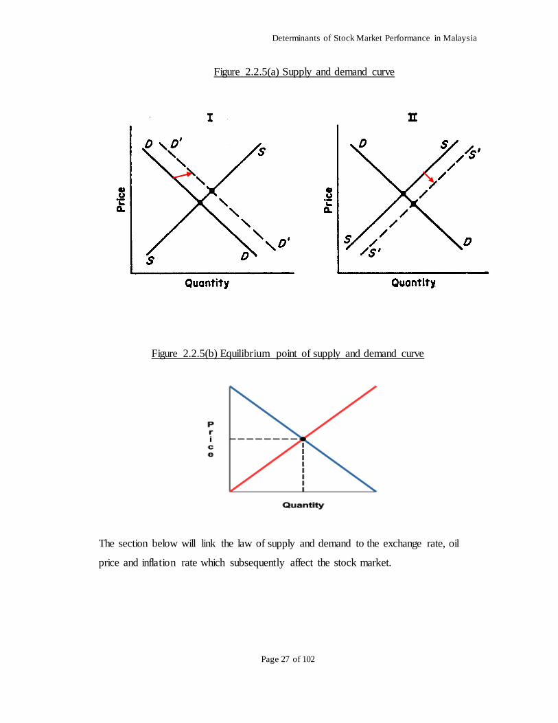
2.2.5 Law of Supply and Demand Theory
Generally, the concept of demand and supply is defined as below in term of its
simplest form (Gale, 1955):
i. If the demand of a good is more than its supply [as shown in Figure 2.2.5(a)],
the price of the good will increase.
ii. If the supply of a good is more than its demand [as shown in Figure 2.2.5(a)],
the price of the good will decrease.
iii. The price will regulate by itself to the value at which the supply and demand
are at the same point. This is known as economic equilibrium [as shown in
Figure 2.2.5(b)].
Determinants of Stock Market Performance in Malaysia
Page 27 of 102
Figure 2.2.5(a) Supply and demand curve
Figure 2.2.5(b) Equilibrium point of supply and demand curve
The section below will link the law of supply and demand to the exchange rate, oil
price and inflation rate which subsequently affect the stock market.
Determinants of Stock Market Performance in Malaysia
Page 28 of 102
2.2.5.1 Exchange Rate
According to Kandil, Berument and Dincer (2007), the exchange rate fluctuation is
affected by its supply and demand. For instance, when the supply of the currency
increases, its value will drop given that the demands of the currency remain
unchanged. There are several ways that the currency can affect the stock price.
When the value of the currency decreases, the foreign investors will deny to
hold the assets of that decline currency because they earn lesser on their
investment return (Dimitrova, 2005). Therefore, the pull out investment from
the foreign investors might imply the company perform weakly and its share
price decreases.
Secondly, the import company might suffer by bearing more costs when the
currency is weak. This is because the company’s costs are higher which
subsequently reduce its revenue. Furthermore, weak revenue might indicate
the poor performance of the company and the share price will drop.
From the perspective of macroeconomic level, a depreciated currency will
improve export industry (Dimitrova, 2005). When the output of the economy
increases, this indicates the economy is booming and the investors will invest
in the stock market.
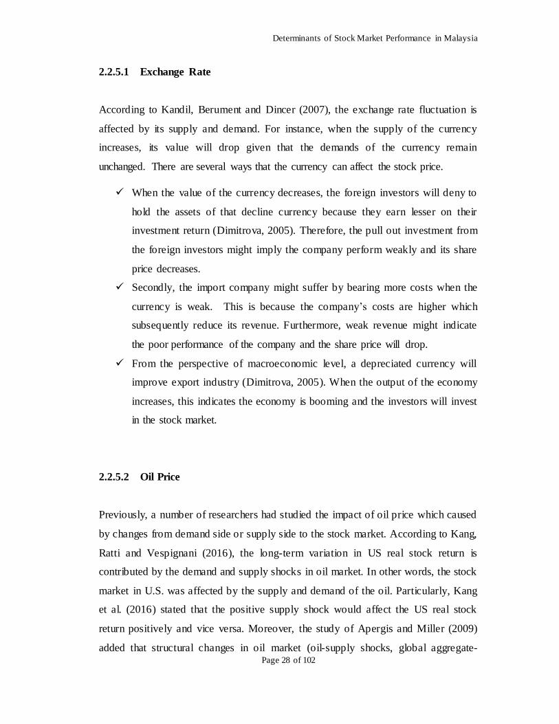
2.2.5.2 Oil Price
Previously, a number of researchers had studied the impact of oil price which caused
by changes from demand side or supply side to the stock market. According to Kang,
Ratti and Vespignani (2016), the long-term variation in US real stock return is
contributed by the demand and supply shocks in oil market. In other words, the stock
market in U.S. was affected by the supply and demand of the oil. Particularly, Kang
et al. (2016) stated that the positive supply shock would affect the US real stock
return positively and vice versa. Moreover, the study of Apergis and Miller (2009)
added that structural changes in oil market (oil-supply shocks, global aggregate-
Determinants of Stock Market Performance in Malaysia
Page 29 of 102
demand shocks, and global oil-demand shocks) would affect the stock market but in a
small magnitude only.
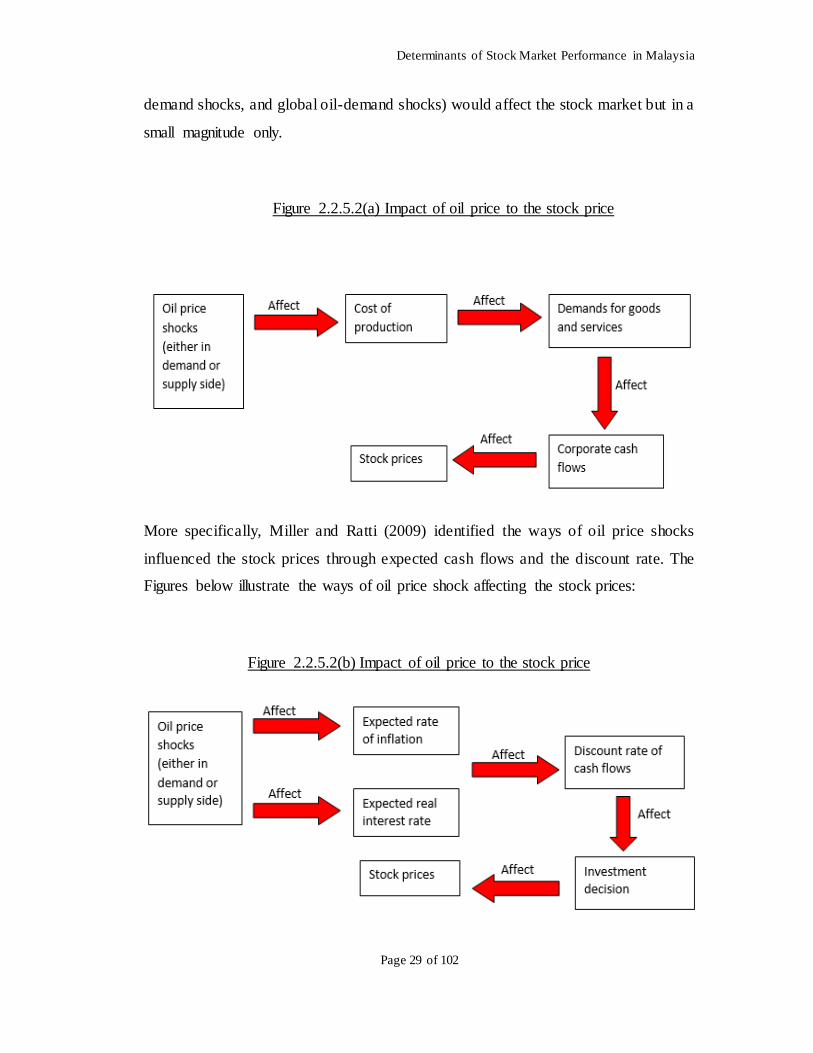
Figure 2.2.5.2(a) Impact of oil price to the stock price
More specifically, Miller and Ratti (2009) identified the ways of oil price shocks
influenced the stock prices through expected cash flows and the discount rate. The
Figures below illustrate the ways of oil price shock affecting the stock prices:
Figure 2.2.5.2(b) Impact of oil price to the stock price
Determinants of Stock Market Performance in Malaysia
Page 30 of 102
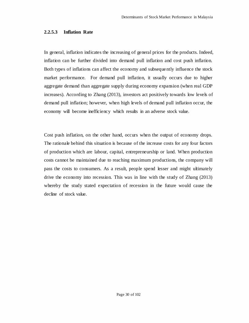
2.2.5.3 Inflation Rate
In general, inflation indicates the increasing of general prices for the products. Indeed,
inflation can be further divided into demand pull inflation and cost push inflation.
Both types of inflations can affect the economy and subsequently influence the stock
market performance. For demand pull inflation, it usually occurs due to higher
aggregate demand than aggregate supply during economy expansion (when real GDP
increases). According to Zhang (2013), investors act positively towards low levels of
demand pull inflation; however, when high levels of demand pull inflation occur, the
economy will become inefficiency which results in an adverse stock value.
Cost push inflation, on the other hand, occurs when the output of economy drops.
The rationale behind this situation is because of the increase costs for any four factors
of production which are labour, capital, entrepreneurship or land. When production
costs cannot be maintained due to reaching maximum productions, the company will
pass the costs to consumers. As a result, people spend lesser and might ultimately
drive the economy into recession. This was in line with the study of Zhang (2013)
whereby the study stated expectation of recession in the future would cause the
decline of stock value.
Determinants of Stock Market Performance in Malaysia
Page 31 of 102
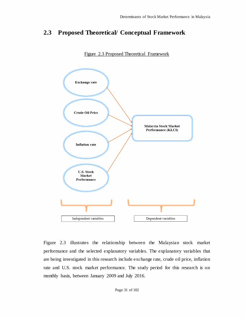
2.3 Proposed Theoretical/ Conceptual Framework
Figure 2.3 Proposed Theoretical Framework
Figure 2.3 illustrates the relationship between the Malaysian stock market
performance and the selected explanatory variables. The explanatory variables that
are being investigated in this research include exchange rate, crude oil price, inflation
rate and U.S. stock market performance. The study period for this research is on
monthly basis, between January 2009 and July 2016.
Determinants of Stock Market Performance in Malaysia
Page 32 of 102
2.4 Hypothesis Development
2.4.1 Exchange Rate
2.4.2 Inflation Rate
2.4.3 US Stock Market Performance
Determinants of Stock Market Performance in Malaysia
Page 33 of 102
2.4.4 Crude Oil Price
2.5 Conclusion
The relationships between the Malaysian stock market performance and each of the
independent variable had been examined in this chapter by summarizing the
methodologies employed by previous researchers. Besides, some of the theoretical
models that have been used in previous studies were discussed in this chapter and
followed by the theoretical framework to demonstrate the relationship between the
dependent variable and independent variables. The methodology used in this study
will be discussed in the following chapter.
Determinants of Stock Market Performance in Malaysia
Page 34 of 102
CHAPTER 3: METHODOLOGY
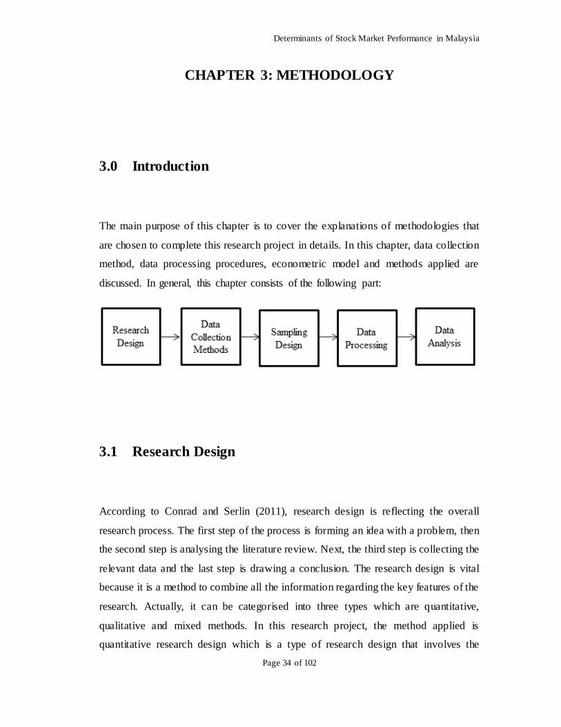
3.0 Introduction
The main purpose of this chapter is to cover the explanations of methodologies that
are chosen to complete this research project in details. In this chapter, data collection
method, data processing procedures, econometric model and methods applied are
discussed. In general, this chapter consists of the following part:
3.1 Research Design
According to Conrad and Serlin (2011), research design is reflecting the overall
research process. The first step of the process is forming an idea with a problem, then
the second step is analysing the literature review. Next, the third step is collecting the
relevant data and the last step is drawing a conclusion. The research design is vital
because it is a method to combine all the information regarding the key features of the
research. Actually, it can be categorised into three types which are quantitative,
qualitative and mixed methods. In this research project, the method applied is
quantitative research design which is a type of research design that involves the
Determinants of Stock Market Performance in Malaysia
Page 35 of 102
numerical and statistical approach. It is specifically based on the existing theor ies,
then conduct the surveys and carry out experiments to answer the research question.
By collecting and processing the data, it provides the result which is more applicable
in the reality.
3.2 Data Collection Methods
The data collected for this study are a monthly time series data from January 2009 to
July 2016. Initially, daily data is planned to use because Palamalai et al. (2013) stated
that by using weekly or monthly data, it will unable to capture the impact of some
responses which last for only a few days. However, CPI does not have daily data.
Thus, monthly data is used instead of yearly data because it enables the sample size to
become larger relative to yearly data.
3.2.1 Secondary Data
Secondary data is chosen for this study. It is a set of data that is collected and readily
available from other sources. This type of data is time saving and inexpensive for data
collection. The table below shows the various sources that accessed for data
collection:
Determinants of Stock Market Performance in Malaysia
Page 36 of 102
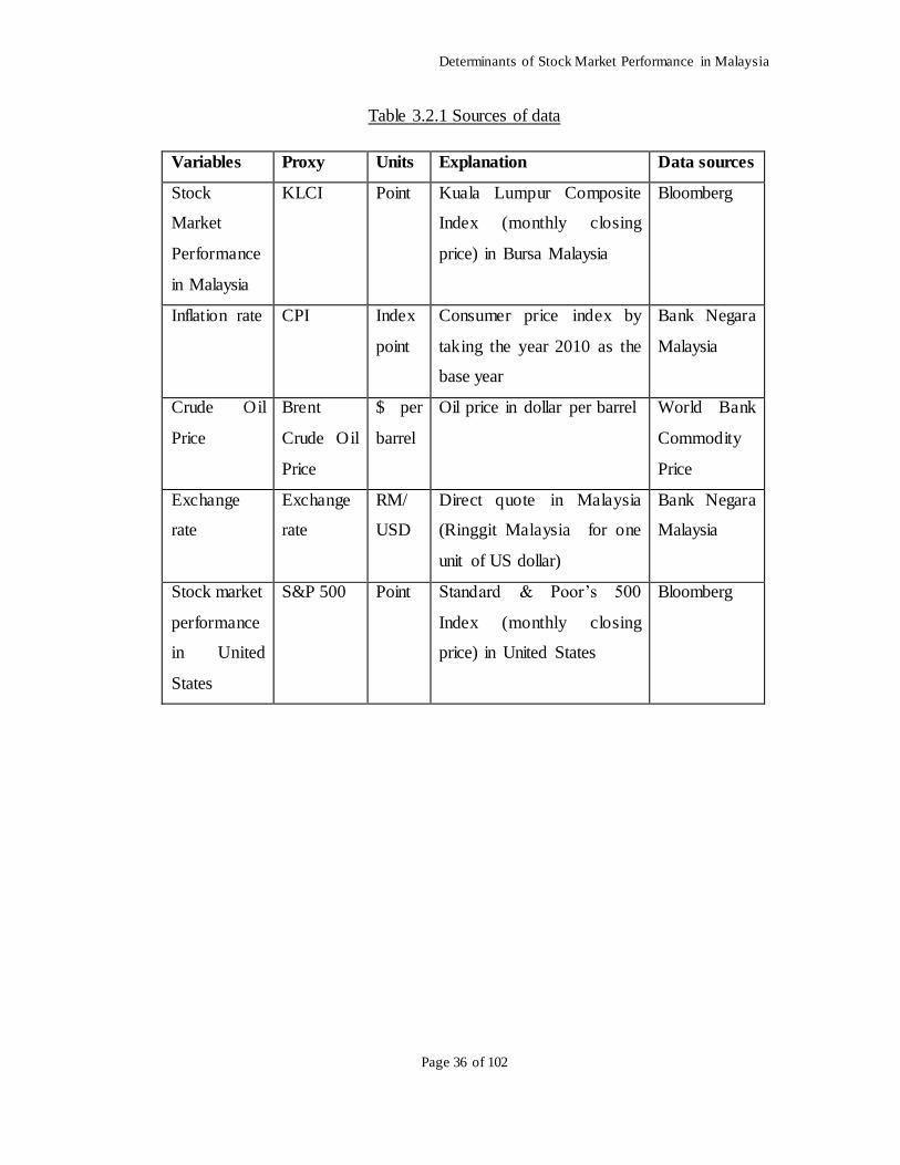
Table 3.2.1 Sources of data
Variables Proxy Units Explanation Data sources
Stock
Market
Performance
in Malaysia
KLCI Point Kuala Lumpur Composite
Index (monthly closing
price) in Bursa Malaysia
Bloomberg
Inflation rate CPI Index
point
Consumer price index by
taking the year 2010 as the
base year
Bank Negara
Malaysia
Crude Oil
Price
Brent
Crude Oil
Price
$ per
barrel
Oil price in dollar per barrel World Bank
Commodity
Price
Exchange
rate
Exchange
rate
RM/
USD
Direct quote in Malaysia
(Ringgit Malaysia for one
unit of US dollar)
Bank Negara
Malaysia
Stock market
performance
in United
States
S&P 500 Point Standard & Poor’s 500
Index (monthly closing
price) in United States
Bloomberg
Determinants of Stock Market Performance in Malaysia
Page 37 of 102
3.3 Sampling Design
3.3.1 Target Population
In this research, Malaysian stock market is set as the target population. In other words,
this research is aimed to determine the relationship of the Kuala Lumpur Composite
Index (KLCI) and the selective variables such as inflation rate (CPI), exchange rate
(RM/USD), crude oil price ($/barrel) and stock market in United State (S&P500)
along the period from January 2009 until July 2016. The reason that KLCI is being
selected as the indicator is due to its high accuracy to represent the Malaysia n stock
market performance as it comprises of thirty largest companies from the main market
in Bursa Malaysia. There are two main eligibility requirements stated in the FTSE
Bursa Malaysia Index Ground Rules which are minimum free float of 15% and
liquidity requirements.
3.3.2 Sample Size
The data of this research is collected in a monthly basis which is from January 2009
to July 2016. A total of 91 observations of data is collected for the dependent variable
Malaysian stock market performance (KLCI) and independent variables such as
inflation rate (CPI), exchange rate, oil price and stock market in US (S&P500). The
sample size of the data in this research is enlarged in o rder to obtain a more accurate
result and to minimize the data omission problem because the missing data can
significantly affect the conclusions that can be drawn from the data.
Determinants of Stock Market Performance in Malaysia
Page 38 of 102
3.3.3 Modification of Original Data for KLCI, S&P 500 and CPI
3.3.3.1 Reasons to log KLCI and S&P500
The reasons to log the proxy of stock market in Malaysia and United States which are
KLCI and S&P500 are as follow:
i. Without transforming the stock market proxy to log form, the model of this
study will meet the problem of wrong functional form. In other words, the
model in this paper is not suitable to study the linear relationship between the
variables and the stock market performance in Malaysia. This is not in line
with the research objective for this study.
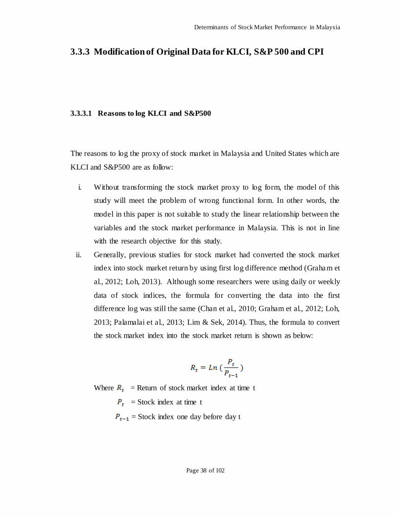
ii. Generally, previous studies for stock market had converted the stock market
index into stock market return by using first log difference method (Graham et
al., 2012; Loh, 2013). Although some researchers were using daily or weekly
data of stock indices, the formula for converting the data into the first
difference log was still the same (Chan et al., 2010; Graham et al., 2012; Loh,
2013; Palamalai et al., 2013; Lim & Sek, 2014). Thus, the formula to convert
the stock market index into the stock market return is shown as below:
Where = Return of stock market index at time t
= Stock index at time t
= Stock index one day before day t
Determinants of Stock Market Performance in Malaysia
Page 39 of 102
3.3.3.2 Re-referencing or Rebasing for CPI
It is important to note that there are several terms refer to the changing of the current
base year to another base year. Australian Bureau of Statistics (ABS) defined re-
referencing as “the process which sets a new index reference period for a price index”
(ABS, 2012b, para. 1).
On the other hand, the United States Census Bureau (2012, para. 4) uses rebasing
instead of re-referencing. They defined rebasing as “a simple method that shifts the
base year from one year to another without changing the base weights for the constant
quality house”. However, both definitions carry the same meaning since ABS (2012a,
para. 6) further mentioning “re-referencing does not change the relative movements
between periods”. In other words, the weightage of a group of basket for measuring
CPI is fixed. Thus, re-referencing and rebasing in this study are referring to changing
the base year of the CPI without revising its weight.
3.3.3.3 Reasons to re-referencing or rebasing CPI
One of the advantages of re-referencing is it allows consistency to exist for a time
series that change over time (Ralph, O’Neill & Winton, 2015). This is important to
ensure the accuracy of the final result for this study. Besides, the United States
Census Bureau (2012, para. 5) stated that “this method assumes that the period-to-
period change (inflation) associated with an old series fairly represents the new series
when new series did not exist”. In other words, re-referencing enables the data to
reflect the current changes of CPI by referring to the latest base year.
Moreover, the index value after re-referencing will still reflect the change of series
between base period and current period, but the initial base year is no longer equal to
100 (Ralph et al., 2015). This indicates the modified data still can reflect the same
impact as the original data.
Determinants of Stock Market Performance in Malaysia
Page 40 of 102
Lastly, the large sample size is obtained by applying re-referencing. As a result, it
enables the variables become normally distributed (Gujarati & Porter, 2009). This is
important as the tests perform in the chapter 4 are based on normal distribution.
Violation of this normality assumption will result in biased result.
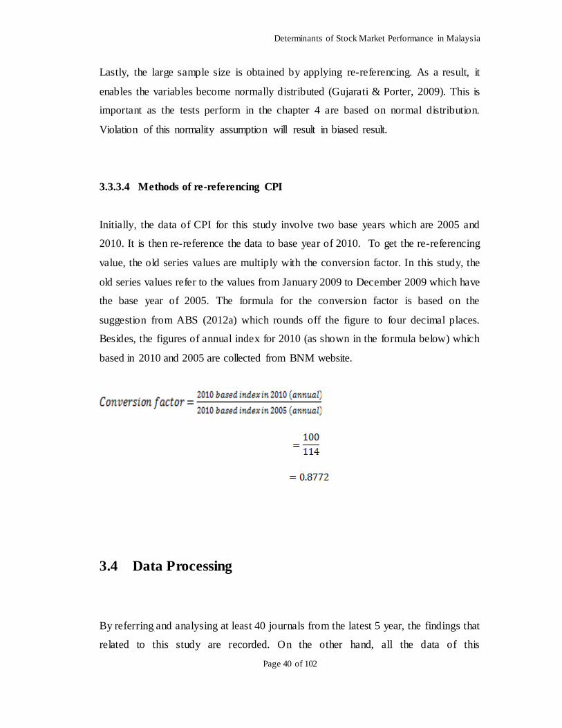
3.3.3.4 Methods of re-referencing CPI
Initially, the data of CPI for this study involve two base years which are 2005 and
2010. It is then re-reference the data to base year of 2010. To get the re-referencing
value, the old series values are multiply with the conversion factor. In this study, the
old series values refer to the values from January 2009 to December 2009 which have
the base year of 2005. The formula for the conversion factor is based on the
suggestion from ABS (2012a) which rounds off the figure to four decimal places.
Besides, the figures of annual index for 2010 (as shown in the formula below) which
based in 2010 and 2005 are collected from BNM website.
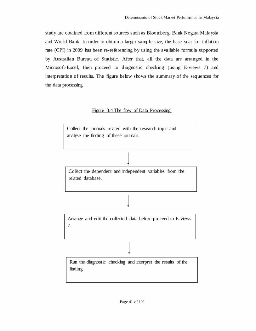
3.4 Data Processing
By referring and analysing at least 40 journals from the latest 5 year, the findings that
related to this study are recorded. On the other hand, all the data of this
Determinants of Stock Market Performance in Malaysia
Page 41 of 102
study are obtained from different sources such as Bloomberg, Bank Negara Malaysia
and World Bank. In order to obtain a larger sample size, the base year for inflation
rate (CPI) in 2009 has been re-referencing by using the available formula supported
by Australian Bureau of Statistic. After that, all the data are arranged in the
Microsoft-Excel, then proceed to diagnostic checking (using E-views 7) and
interpretation of results. The figure below shows the summary of the sequences for
the data processing.
Figure 3.4 The flow of Data Processing.
Run the diagnostic checking and interpret the results of the
finding.
Collect the journals related with the research topic and
analyse the finding of these journals.
Collect the dependent and independent variables from the
related database.
Arrange and edit the collected data before proceed to E-views
7.
Determinants of Stock Market Performance in Malaysia
Page 42 of 102
3.5 Data Analysis
3.5.1 Multiple Linear Regression Model
According to Cohen, Cohen, West and Aiken (2003), Multiple Linear Regression
Model is a model that contains two or more independent variables to predict the
determinants’ impact on the dependent variable. Gujarati and Porter (2009) showed
that there are few assumptions that the model has to follow in order to get Best Linear
Unbiased Efficient Estimator (BLUE) results. BLUE can be explained as all the
estimators must be in linear form with a minimum error of estimation. Besides, the
expected value of coefficients are equal or near to the true value and the model
consists of minimum variance.
In some studies, some of the variables will be transformed into logarithm form.
Indeed, log transformation of variables can decrease the variation of the data
(Imarhiagbe, 2010). Besides, Wooldridge (2005) shows that the independent variable
in logarithm is approximately to the assumptions of classical linear regression model.
The model in this study is as follow:
lnKLCI = f [Exchange Rate (EXR), Consumer Price Index (CPI), S&P 500 Index
(SPX), Crude Oil Price (OIL)]
Determinants of Stock Market Performance in Malaysia
Page 43 of 102
Economic Function:
lnYt = β0 + β1Xt + β2Xt + β3lnXt + β4Xt + εt
lnKLCIt = B0 + B1 EXRt + B2 CPIt + B3 lnSPXt + B4 OILt + εt
Where:
lnKLCIt = The natural logarithm form of Kuala Lumpur Composite Index
(KLCI) at year t. (%)
EXRt = Exchange Rate (EXR) at year t. (RM/USD)
CPIt = Consumer Price Index (CPI) at year t. (Index point)
lnSPXt = The natural logarithm of S&P 500 Index (SPX) at year t. (%)
OILt = Oil Price (OIL) at year t. ($ per barrel)
εt = Error term
3.5.2 Ordinary Least-Square
Ordinary Least-Square (OLS) regression is a generalized linear modelling technique
which is used to estimate the figures of the parameters in order to fit a function to a
set of data. OLS regression is widely used and can be easily adapted to include a
number of explanatory variables, including dummy variables (Hutcheson & Moutinho,
2011). In other words, OLS regression is applicable to a single explanatory variable,
multiple explanatory variables, and categorical explanatory variables.
Determinants of Stock Market Performance in Malaysia
Page 44 of 102
According to Hutcheson and Sofroniou (1999), the OLS regression is powerful as it
can trace the model assumptions in its linearity, constant variance and the effect of
outliers by using simple graphical methods. However, the Gauss-Markov theorem
stated that there are five conditions to be fulfilled in order to obtain the smallest
variance (Wooldridge, 2013). The five conditions of Gauss-Markov theorem are
listed as below:
1. The regression model is linear in parameters.
2. The observations are random sampling.
3. There are no exact linear relationships among the independent variables.
4. The error term has a zero mean value.
5. The error term is homoscedasticity.
In other words, once the OLS estimates are fulfilling the stated five Gauss-Markov
conditions, the OLS estimators are the best linear unbiased estimators.
3.5.3 E-Views 7
E-Views is a spreadsheet software that used for various types of data analysis. It has
some similarity to the commonly used Microsoft Excel and does support this type of
files. In fact, it is a sophisticated software for analysing data, forming regression line,
and forecasting in computers operating in Microsoft Windows. It will not be possible
if researchers intend to conduct analysis without using E-Views. Since E-Views is a
tool which designed for economic purposes, it is useful for analysing economic time
series and even for handling a quite large cross-section projects. Besides, E-Views is
designed to provide convenient visual ways to enter data series from disk files, to
create new series from existing ones, to display and print series, and to carry out
statistical analysis of the relationships among series.
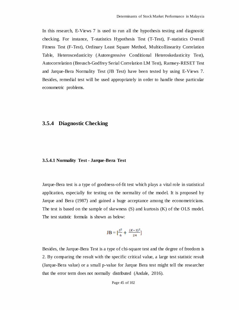
Determinants of Stock Market Performance in Malaysia
Page 45 of 102
In this research, E-Views 7 is used to run all the hypothesis testing and diagnostic
checking. For instance, T-statistics Hypothesis Test (T-Test), F-statistics Overall
Fitness Test (F-Test), Ordinary Least Square Method, Multicollinearity Correlation
Table, Heteroscedasticity (Autoregressive Conditional Heteroskedasticity Test),
Autocorrelation (Breusch-Godfrey Serial Correlation LM Test), Ramsey-RESET Test
and Jarque-Bera Normality Test (JB Test) have been tested by using E-Views 7.
Besides, remedial test will be used appropriately in order to handle those particular
econometric problems.
3.5.4 Diagnostic Checking
3.5.4.1 Normality Test - Jarque-Bera Test
Jarque-Bera test is a type of goodness-of-fit test which plays a vital role in statistical
application, especially for testing on the normality of the model. It is proposed by
Jarque and Bera (1987) and gained a huge acceptance among the econometricians.
The test is based on the sample of skewness (S) and kurtosis (K) of the OLS model.
The test statistic formula is shown as below:
Besides, the Jarque-Bera Test is a type of chi-square test and the degree of freedom is
2. By comparing the result with the specific critical value, a large test statistic result
(Jarque-Bera value) or a small p-value for Jarque Bera test might tell the researcher
that the error term does not normally distributed (Andale, 2016).
Determinants of Stock Market Performance in Malaysia
Page 46 of 102
3.5.4.2 Model Specification
According to Gujarati and Porter (2009), model specification error is an econometric
problem where the model consists of any one or combination of the situations below:
i) Omitting important or relevant variables.
ii) Including irrelevant variables.
iii) Existing of wrong functional in the model.
Model specification errors will cause the outcome of the studies to become
inconsistent with the theoretical expectation (Jarvis, Mackenzie & Podsakoff, 2003).
Hence, having this problem will disobey the assumption of CLRM.
In order to detect the model specification errors, performing Ramsey Reset Test is
one of the methods to compute the stability of specification error. RESET stands for
Regression Specification Error Test, and it tests whether the non-linear combinations
of the fitted values help to explain the response variable (Wooldridge, 2005). RESET
test will be used in this study.
Determinants of Stock Market Performance in Malaysia
Page 47 of 102
3.5.4.3 Multicollinearity
Multicollinearity problem occurs when there are two or more explanatory variables
are highly correlated with each other in a multiple regression model (Adeboye,
Fagoyinbo & Olatayo, 2014). According to Vatcheva, Lee, McCormick and Rahbar
(2016), the reason that multicollinearity problem occurs in the model is due to the
population unrepresentative sample or insufficient information in the sample.
In the presence of multicollinearity, the regression model has difficulty in
determining which explanatory variables are influencing the dependent variable.
There are few consequences of multicollinearity problem in a regression model.
Firstly, the variances of ordinary least square (OLS) estimators will become larger
which result in less precise in the estimation. Secondly, the confident intervals
become much wider and this results in more easily to accept the null hypothesis.
Thirdly, the t-ratios of the coefficients are more likely to be insignificant due to the
wider confidence interval while the R-square for the model with multicollinearity
could still be relatively high which results in invalid hypothesis testing. Nonetheless,
the model with multicollinearity does not violate OLS assumptions; the OLS
estimates are still Best Linear Unbiased Estimators.
There are several ways to detect the presence of multicollinearity problem in a model.
Firstly, the multicollinearity problem is suspected if there are few significant t-ratios
for the individual coefficients with the overall significant F-statistic. Secondly, a high
pair-wise correlation coefficient also indicates that the model is suspected to have a
multicollinearity problem. Indeed, Yu, Jiang and Land (2015) suggest that when the
pair-wise correlation coefficient is equal to 0.7 or higher, the model is suspected to
have a multicollinearity problem.
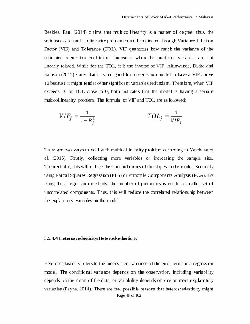
Determinants of Stock Market Performance in Malaysia
Page 48 of 102
Besides, Paul (2014) claims that multicollinearity is a matter of degree; thus, the
seriousness of multicollinearity problem could be detected through Variance Inflation
Factor (VIF) and Tolerance (TOL). VIF quantifies how much the variance of the
estimated regression coefficients increases when the predictor variables are not
linearly related. While for the TOL, it is the inverse of VIF. Akinwande, Dikko and
Samson (2015) states that it is not good for a regression model to have a VIF above
10 because it might render other significant variables redundant. Therefore, when VIF
exceeds 10 or TOL close to 0, both indicates that the model is having a serious
multicollinearity problem. The formula of VIF and TOL are as followed:
= =
There are two ways to deal with multicollinearity problem according to Vatcheva et
al. (2016). Firstly, collecting more variables or increasing the sample size.
Theoretically, this will reduce the standard errors of the slopes in the model. Secondly,
using Partial Squares Regression (PLS) or Principle Components Analysis (PCA). By
using these regression methods, the number of predictors is cut to a smaller set of
uncorrelated components. Thus, this will reduce the correlated relationship between
the explanatory variables in the model.
3.5.4.4 Heteroscedasticity/Heteroskedasticity
Heteroscedasticity refers to the inconsistent variance of the error terms in a regression
model. The conditional variance depends on the observation, including variability
depends on the mean of the data, or variability depends on one or more explanatory
variables (Payne, 2014). There are few possible reasons that heteroscedasticity might
Determinants of Stock Market Performance in Malaysia
Page 49 of 102
be occurred in the model. Firstly, there is a measurement error where there might be a
possibility that the respondents are giving less accurate responses than others during
data collection. Secondly, a model misspecification is detected where the model is not
correctly specified due to omitted variables or includes non-related variables in the
model.
The present of heteroscedasticity in the model will lead to several consequences.
Firstly, the Ordinary Least Square (OLS) estimates are no longer Best Linear
Unbiased Estimators. The OLS method is inefficient because it violates the
assumption of minimum variance of the error terms. Secondly, the variances and
standard errors of a model are underestimated. Inaccurate standard errors will tend to
increase the value of t-statistic and f-statistic; thus, the hypothesis testing of T-
statistic and F-statistic are no longer valid. However, the OLS estimators for the
coefficients are still unbiased and consistent since the explanatory variables are
uncorrelated to the error terms (Gujarati & Porter, 2009).
According to Gujarati and Porter (2009), there are two ways to detect the presence of
heteroscedasticity in general which are the informal way and the formal way. The
informal way could be carried out through the graphical method, while the formal
way could be carried out through several formal tests such as the Breusch-Pagan LM
test, Glesjer LM test, Harvey-Godfrey LM test, Park LM test, Goldfeld-Quandt test,
ARCH test and White’s test. However, Wong (2014) specifies that Autoregressive
Conditional Heteroskedasticity (ARCH) model is used in order to detect the
heteroskedasticity problem for time-series data.
There are three ways to deal with heteroscedasticity problem according to Williams
(2015) which are transforming the variables, using Robust Standard Errors and
Weighted Least Squares (WLS) method. WLS method is the most suitable solution
Determinants of Stock Market Performance in Malaysia
Page 50 of 102
for heteroscedasticity problem providing that the pattern of the error variances are
known (Gujarati & Porter, 2009).
In this study, ARCH Test is applied to test the time series data. The hypotheses for
this test are stated as below:
3.5.4.5 Autocorrelation
According to Gujarati and Porter (2009), autocorrelation problem is defined as a
problem exists when the random variable which ordered over time shows nonzero
covariance. It can be explained as there is a relationship among error terms. Having
autocorrelation problem is the violation of CLRM’s assumption. There are several
consequences for the existing of autocorrelation problem (Greene, 2003).
a) OLS estimators are still unbiased and linear. However, minimum variance
property is not satisfied.
b) Confidence intervals and hypothesis test based on t and F distributions are
unreliable. There is a possibility of drawing a wrong conclusion on hypothesis
tests.
c) If the disturbance terms, ui are correlated, then the OLS estimates are non-
asymptotic. The variance of random term might be seriously underestimated.
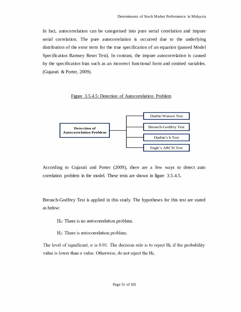
Determinants of Stock Market Performance in Malaysia
Page 51 of 102
In fact, autocorrelation can be categorised into pure serial correlation and impure
serial correlation. The pure autocorrelation is occurred due to the underlying
distribution of the error term for the true specification of an equation (passed Model
Specification Ramsey Reset Test). In contrast, the impure autocorrelation is caused
by the specification bias such as an incorrect functional form and omitted variables.
(Gujarati & Porter, 2009).
Figure 3.5.4.5: Detection of Autocorrelation Problem
Durbin Watson Test
Detection of
Autocorrelation Problem
Engle’s ARCH Test
Durbin’s h Test
Breusch-Godfrey Test
According to Gujarati and Porter (2009), there are a few ways to detect auto
correlation problem in the model. These tests are shown in figure 3.5.4.5.
Breusch-Godfrey Test is applied in this study. The hypotheses for this test are stated
as below:
Determinants of Stock Market Performance in Malaysia
Page 52 of 102
3.5.5 F-statistic test
F-statistic test was created by George W. Snedecor and developed by Sir Ronald A.
Fisher in 1920 (Jeffrey, James, Michael, Jeffrey & David, 2015). An F-test is any
statistical test in which the test statistic has an F-distribution under the null hypothesis.
It is most often used when comparing statistical models that have been fitted to a data
set in order to identify the model that best fits the population from which the data are
sampled. In other words, it is used to test the overall fitness of the model.
Furthermore, F-statistic test can be conducted by using E-Views 7 and the value can
be generated from the equation window and the P-value of F-statistic test can be
generated from the output (Gujarati & Porter, 2009).
The null hypothesis and alternative hypothesis for this test are stated as below:
Reject H0 if the F-statistic value is lower than critical value at significant level
(assume = 0.01). Otherwise, do not reject H0.
Reject H0 if the P-value is smaller than the significant level (assume = 0.01).
Otherwise, do not reject H0.
3.5.6 T-statistic test
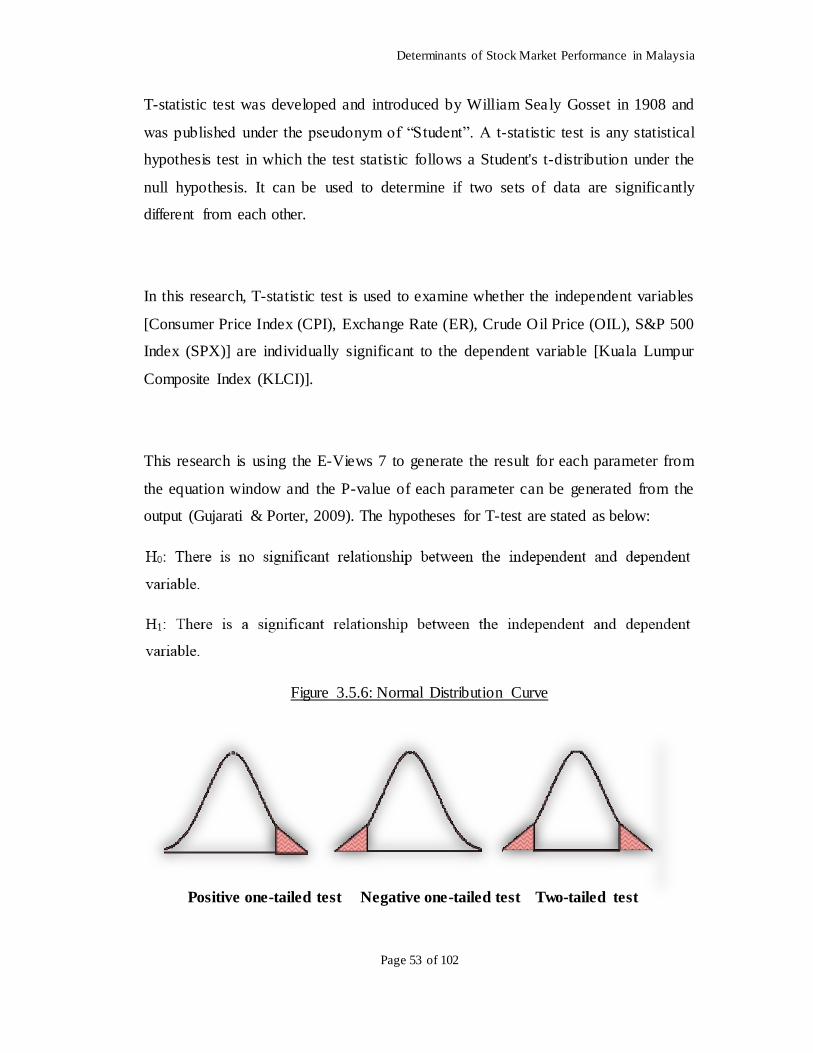
Determinants of Stock Market Performance in Malaysia
Page 53 of 102
T-statistic test was developed and introduced by William Sealy Gosset in 1908 and
was published under the pseudonym of “Student”. A t-statistic test is any statistical
hypothesis test in which the test statistic follows a Student's t-distribution under the
null hypothesis. It can be used to determine if two sets of data are significantly
different from each other.
In this research, T-statistic test is used to examine whether the independent variables
[Consumer Price Index (CPI), Exchange Rate (ER), Crude Oil Price (OIL), S&P 500
Index (SPX)] are individually significant to the dependent variable [Kuala Lumpur
Composite Index (KLCI)].
This research is using the E-Views 7 to generate the result for each parameter from
the equation window and the P-value of each parameter can be generated from the
output (Gujarati & Porter, 2009). The hypotheses for T-test are stated as below:
Figure 3.5.6: Normal Distribution Curve
Positive one-tailed test Negative one-tailed test Two-tailed test
Determinants of Stock Market Performance in Malaysia
Page 54 of 102
3.6 Conclusion
In conclusion, Chapter 3 has included detail explanations on research design, data
collection methods, sampling design, data processing and data analysis. This chapter
clearly stated out the econometric model that will be applied in this research. Last but
not least, this chapter also covered and provided explanations for all econometric
methods and statistical tests applied in this research. The empirical result of these
tests will be conducted in the following chapter.
Determinants of Stock Market Performance in Malaysia
Page 55 of 102
CHAPTER 4: DATA ANALYSIS
4.0 Introduction
This chapter focuses on interpreting the empirical results generating from Eview
software. The involved tests are Ordinary Least Squares (OLS) method, T-Test, F-
Test, Normality Test, and four diagnostic checking including Multicollinearity,
Heteroscedasticity, Autocorrelation and Model Specification. All the results will be
expressed in a table form and followed by the respective interpretations.
4.1 Diagnostic Checking
4.1.1 Normality Test
Jarque-Bera test is a type of goodness-of-fit test which plays a vital role in statistical
application, especially for testing on the normality of the model.
Determinants of Stock Market Performance in Malaysia
Page 56 of 102
4.1.2 Model Specification
Ramsey Reset Test is one of the methods to compute the stability of specification
error. Having model specification problem will make the result of the study become
inconsistent with the theoretical expectation.
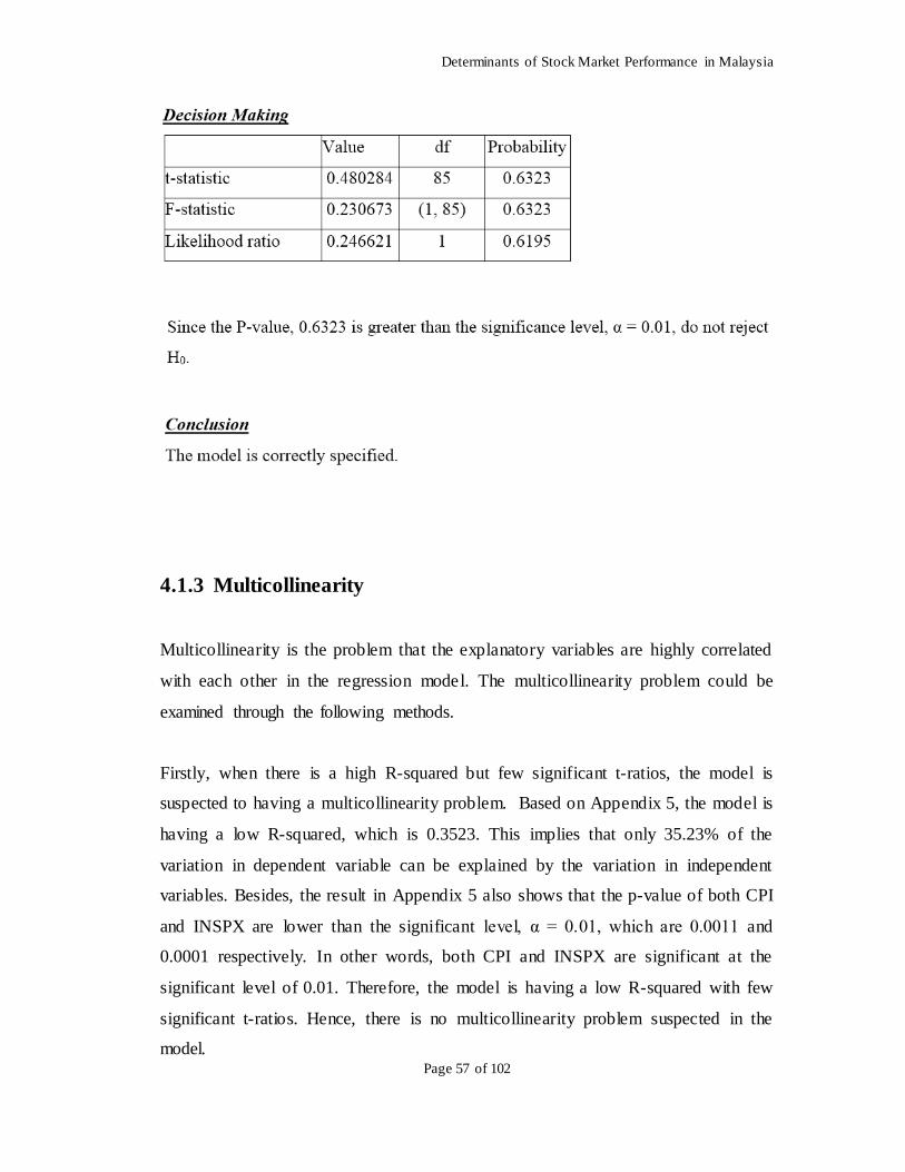
Determinants of Stock Market Performance in Malaysia
Page 57 of 102
4.1.3 Multicollinearity
Multicollinearity is the problem that the explanatory variables are highly correlated
with each other in the regression model. The multicollinearity problem could be
examined through the following methods.
Firstly, when there is a high R-squared but few significant t-ratios, the model is
suspected to having a multicollinearity problem. Based on Appendix 5, the model is
having a low R-squared, which is 0.3523. This implies that only 35.23% of the
variation in dependent variable can be explained by the variation in independent
variables. Besides, the result in Appendix 5 also shows that the p-value of both CPI
and INSPX are lower than the significant level, α = 0.01, which are 0.0011 and
0.0001 respectively. In other words, both CPI and INSPX are significant at the
significant level of 0.01. Therefore, the model is having a low R-squared with few
significant t-ratios. Hence, there is no multicollinearity problem suspected in the
model.
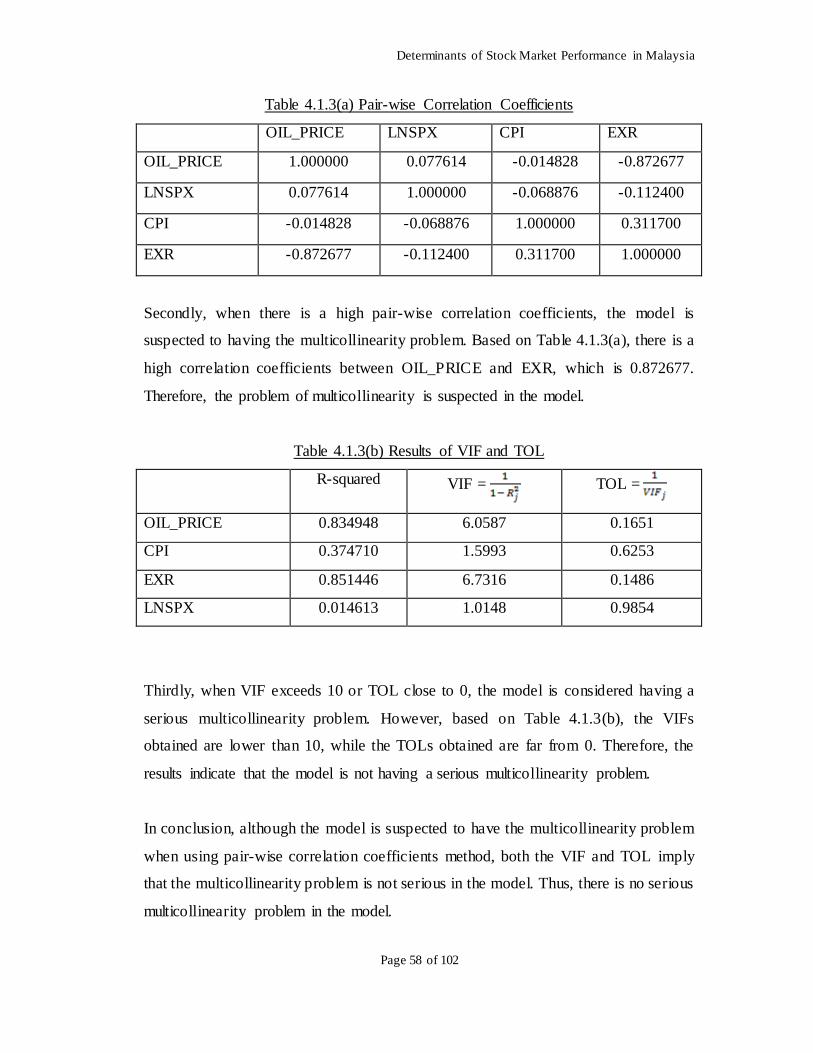
Determinants of Stock Market Performance in Malaysia
Page 58 of 102
Table 4.1.3(a) Pair-wise Correlation Coefficients
OIL_PRICE LNSPX CPI EXR
OIL_PRICE 1.000000 0.077614 -0.014828 -0.872677
LNSPX 0.077614 1.000000 -0.068876 -0.112400
CPI -0.014828 -0.068876 1.000000 0.311700
EXR -0.872677 -0.112400 0.311700 1.000000
Secondly, when there is a high pair-wise correlation coefficients, the model is
suspected to having the multicollinearity problem. Based on Table 4.1.3(a), there is a
high correlation coefficients between OIL_PRICE and EXR, which is 0.872677.
Therefore, the problem of multicollinearity is suspected in the model.
Table 4.1.3(b) Results of VIF and TOL
R-squared VIF = TOL =
OIL_PRICE 0.834948 6.0587 0.1651
CPI 0.374710 1.5993 0.6253
EXR 0.851446 6.7316 0.1486
LNSPX 0.014613 1.0148 0.9854
Thirdly, when VIF exceeds 10 or TOL close to 0, the model is considered having a
serious multicollinearity problem. However, based on Table 4.1.3(b), the VIFs
obtained are lower than 10, while the TOLs obtained are far from 0. Therefore, the
results indicate that the model is not having a serious multicollinearity problem.
In conclusion, although the model is suspected to have the multicollinearity problem
when using pair-wise correlation coefficients method, both the VIF and TOL imply
that the multicollinearity problem is not serious in the model. Thus, there is no serious
multicollinearity problem in the model.
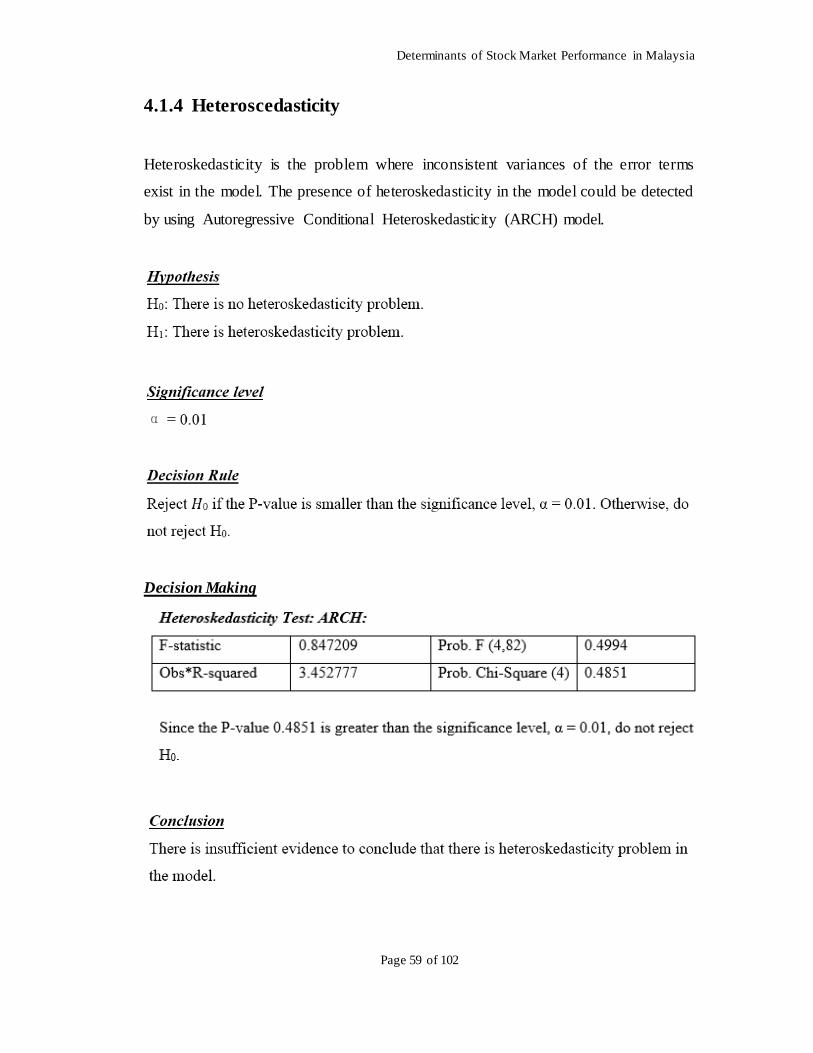
Determinants of Stock Market Performance in Malaysia
Page 59 of 102
4.1.4 Heteroscedasticity
Heteroskedasticity is the problem where inconsistent variances of the error terms
exist in the model. The presence of heteroskedasticity in the model could be detected
by using Autoregressive Conditional Heteroskedasticity (ARCH) model.
Decision Making
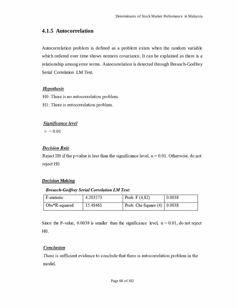
Determinants of Stock Market Performance in Malaysia
Page 60 of 102
4.1.5 Autocorrelation
Autocorrelation problem is defined as a problem exists when the random variable
which ordered over time shows nonzero covariance. It can be explained as there is a
relationship among error terms. Autocorrelation is detected through Breusch-Godfrey
Serial Correlation LM Test.
Decision Making
Since the P-value, 0.0038 is smaller than the significance level, α = 0.01, do not reject
H0.
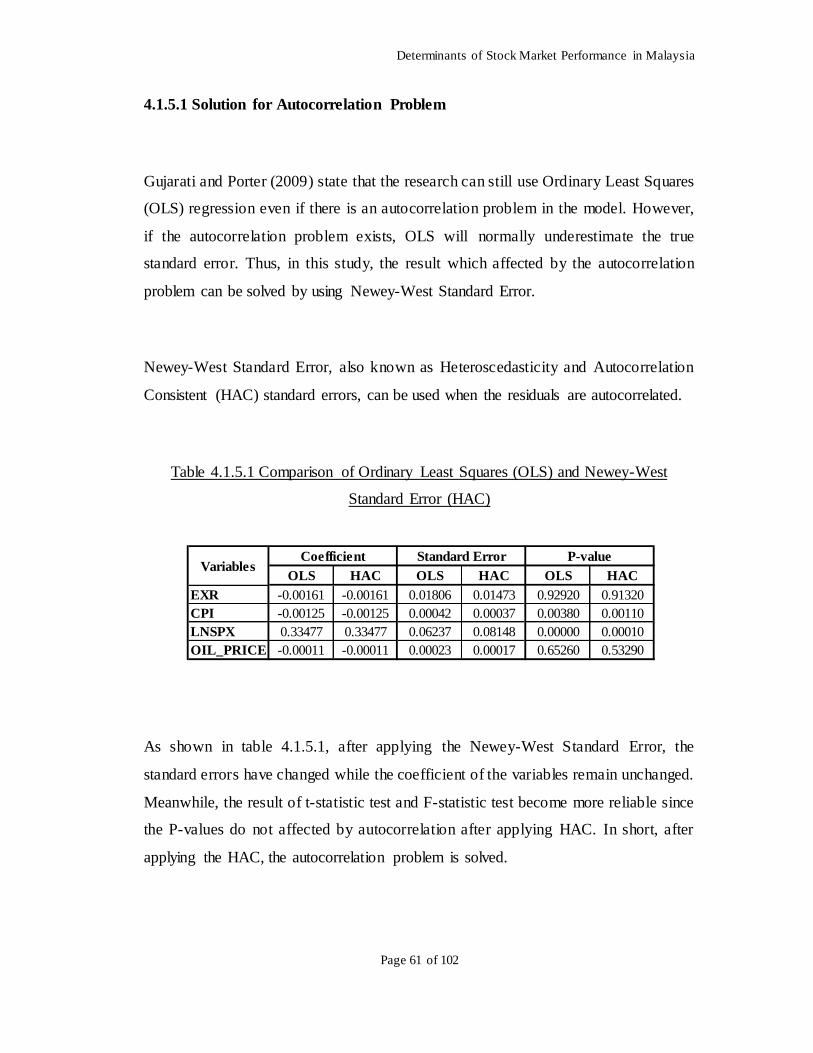
Determinants of Stock Market Performance in Malaysia
Page 61 of 102
4.1.5.1 Solution for Autocorrelation Problem
Gujarati and Porter (2009) state that the research can still use Ordinary Least Squares
(OLS) regression even if there is an autocorrelation problem in the model. However,
if the autocorrelation problem exists, OLS will normally underestimate the true
standard error. Thus, in this study, the result which affected by the autocorrelation
problem can be solved by using Newey-West Standard Error.
Newey-West Standard Error, also known as Heteroscedasticity and Autocorrelation
Consistent (HAC) standard errors, can be used when the residuals are autocorrelated.
Table 4.1.5.1 Comparison of Ordinary Least Squares (OLS) and Newey-West
Standard Error (HAC)
OLS HAC OLS HAC OLS HAC
EXR -0.00161 -0.00161 0.01806 0.01473 0.92920 0.91320
CPI -0.00125 -0.00125 0.00042 0.00037 0.00380 0.00110
LNSPX 0.33477 0.33477 0.06237 0.08148 0.00000 0.00010
OIL_PRICE -0.00011 -0.00011 0.00023 0.00017 0.65260 0.53290
P-valueStandard ErrorCoefficientVariables
As shown in table 4.1.5.1, after applying the Newey-West Standard Error, the
standard errors have changed while the coefficient of the variables remain unchanged.
Meanwhile, the result of t-statistic test and F-statistic test become more reliable since
the P-values do not affected by autocorrelation after applying HAC. In short, after
applying the HAC, the autocorrelation problem is solved.
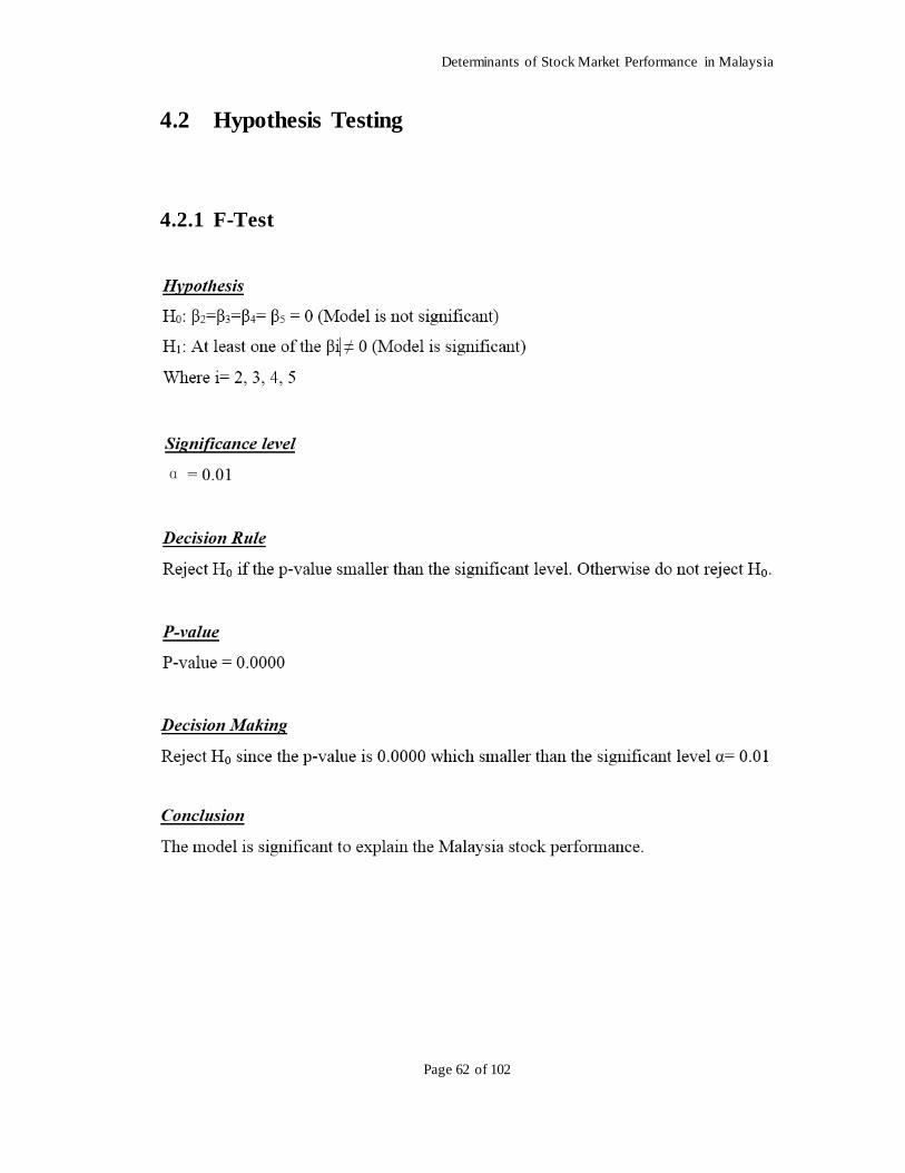
Determinants of Stock Market Performance in Malaysia
Page 62 of 102
4.2 Hypothesis Testing
4.2.1 F-Test
Determinants of Stock Market Performance in Malaysia
Page 63 of 102
4.2.2 T-test
This research uses t-test with p-value approach at significant level of 0.01 to examine
whether each independent variable is significant or not. Below are the general
hypotheses and decision rules for the t-test:
4.2.2.1 Exchange Rate (EXR)
Determinants of Stock Market Performance in Malaysia
Page 64 of 102
4.2.2.2 Consumer Price Index (CPI)
4.2.2.3 S&P 500 Index (SPX)
Determinants of Stock Market Performance in Malaysia
Page 65 of 102
4.2.2.4 Crude Oil Price (OIL)
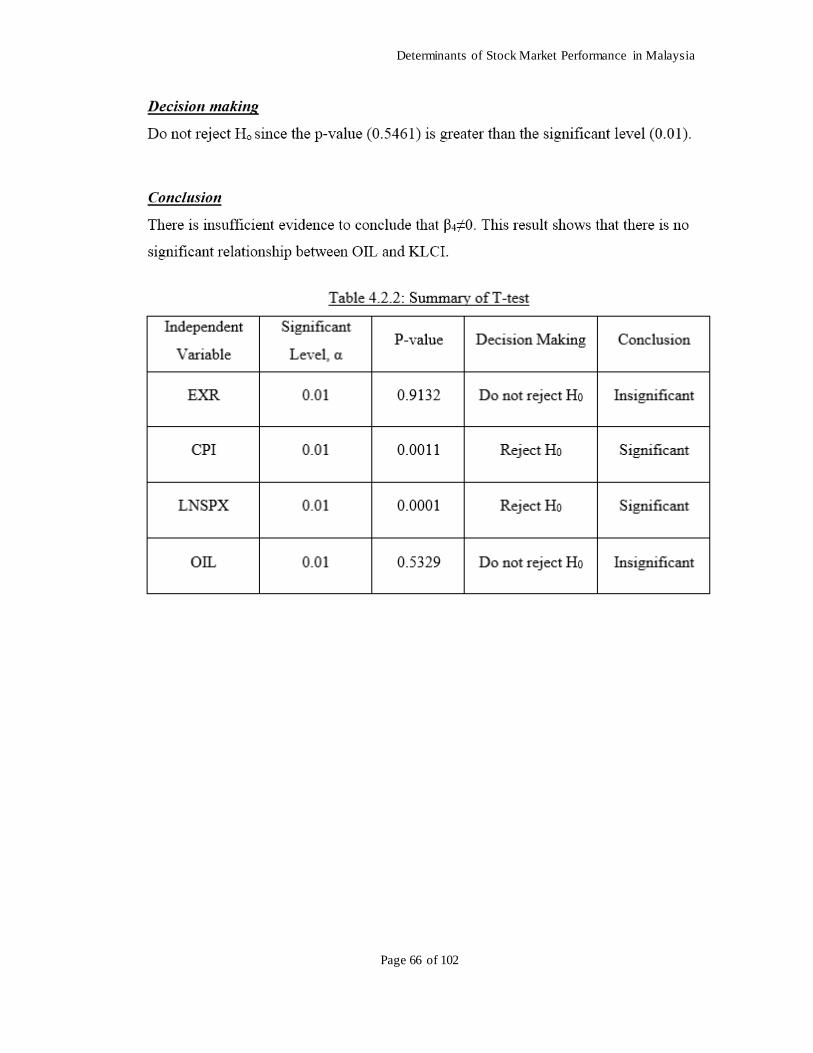
Determinants of Stock Market Performance in Malaysia
Page 66 of 102
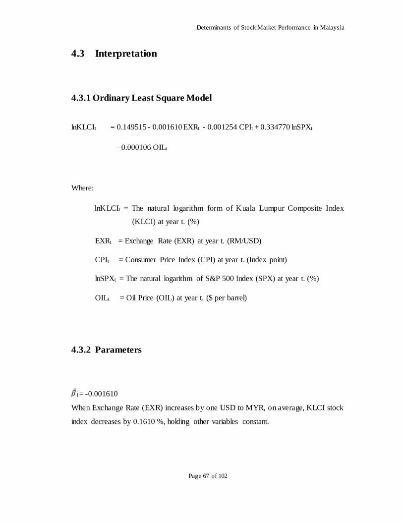
Determinants of Stock Market Performance in Malaysia
Page 67 of 102
4.3 Interpretation
4.3.1 Ordinary Least Square Model
lnKLCIt = 0.149515 - 0.001610 EXRt - 0.001254 CPIt + 0.334770 lnSPXt
- 0.000106 OILt
Where:
lnKLCIt = The natural logarithm form of Kuala Lumpur Composite Index
(KLCI) at year t. (%)
EXRt = Exchange Rate (EXR) at year t. (RM/USD)
CPIt = Consumer Price Index (CPI) at year t. (Index point)
lnSPXt = The natural logarithm of S&P 500 Index (SPX) at year t. (%)
OILt = Oil Price (OIL) at year t. ($ per barrel)
4.3.2 Parameters
1= -0.001610
When Exchange Rate (EXR) increases by one USD to MYR, on average, KLCI stock
index decreases by 0.1610 %, holding other variables constant.
Determinants of Stock Market Performance in Malaysia
Page 68 of 102
2 = -0.001254
When Consumer Price Index (CPI) increases by 1 index point, on average, KLCI
stock index decreases by 0.1254 %, holding other variables constant.
3= 0.334770
When S&P 500 Index (SPX) increases by 1%, on average, KLCI stock index
increases by 0.334770 %, holding other variables constant.
4 = -0.000106
When Oil Price (OIL) increases by $ 1 per barrel, on average, KLCI stock index
decreases by 0.0106%, holding other variables constant.
4.3.3 Goodness of fit
Goodness of fit is shown by the R2 in the eview result.
R2 = 0.352294: There is 35.23% of the variation in log of KLCI can be explained by
the exchange rate, oil price, CPI and log of SPX.
Adjusted R2 = 0.322168: There is 32.22% of the variation in log of KLCI can be
explained by the exchange rate, oil price, CPI and log of SPX, after taking into
account the degrees of freedom (the sample size and the number of independent
variable, n-k-1).
Determinants of Stock Market Performance in Malaysia
Page 69 of 102
4.4 Conclusion
In this chapter, the relationships between Malaysian stock market performance and
four determinants are examined. Several diagnostic checking tests such as Jarque-
Bera test (Normality), Ramsey Reset (Model Misspecification) test, Multicollinearity
Test, Autoregressive Conditional Heteroskedasticity (ARCH) test and Breusch-
Godfrey Serial Correlation LM Test (Autocorrelation) have been conducted in this
study. The autocorrelation problem has been overcome by using the Newey-West
Standard Error. In the next chapter, the summary for the whole research will be
discussed.
Determinants of Stock Market Performance in Malaysia
Page 70 of 102
CHAPTER 5: DISCUSSION, CONCLUSION AND
IMPLICATION
5.0 Introduction
Results from Chapter 4 had showed the relationship between the Malaysian stock
market performance and the four independent variables which are inflation rate (CPI),
exchange rate, crude oil price and the US stock market performance (S&P500 index).
The first section of this chapter is the summary of the result from the diagnostic
checking computed in the previous chapter. The second section is the summary and
the discussion on the relationship of the major findings in this study. The third section
of this chapter will suggest the policy implication for different sectors. The fourth
section will discuss about the limitation faces in this study, then follows by the related
recommendation for the future study. Lastly, this chapter ends with a conclusion
which summaries the contents in this chapter.
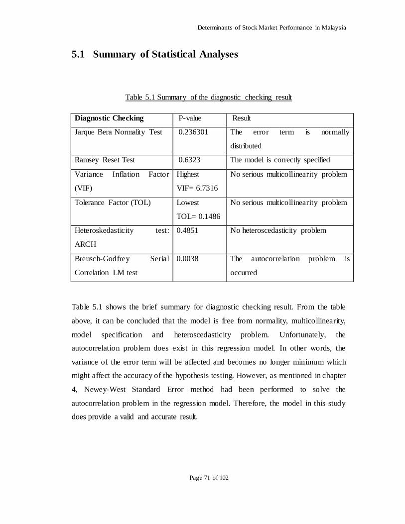
Determinants of Stock Market Performance in Malaysia
Page 71 of 102
5.1 Summary of Statistical Analyses
Table 5.1 Summary of the diagnostic checking result
Diagnostic Checking P-value Result
Jarque Bera Normality Test 0.236301 The error term is normally
distributed
Ramsey Reset Test 0.6323 The model is correctly specified
Variance Inflation Factor
(VIF)
Highest
VIF= 6.7316
No serious multicollinearity problem
Tolerance Factor (TOL) Lowest
TOL= 0.1486
No serious multicollinearity problem
Heteroskedasticity test:
ARCH
0.4851 No heteroscedasticity problem
Breusch-Godfrey Serial
Correlation LM test
0.0038 The autocorrelation problem is
occurred
Table 5.1 shows the brief summary for diagnostic checking result. From the table
above, it can be concluded that the model is free from normality, multicollinearity,
model specification and heteroscedasticity problem. Unfortunately, the
autocorrelation problem does exist in this regression model. In other words, the
variance of the error term will be affected and becomes no longer minimum which
might affect the accuracy of the hypothesis testing. However, as mentioned in chapter
4, Newey-West Standard Error method had been performed to solve the
autocorrelation problem in the regression model. Therefore, the model in this study
does provide a valid and accurate result.
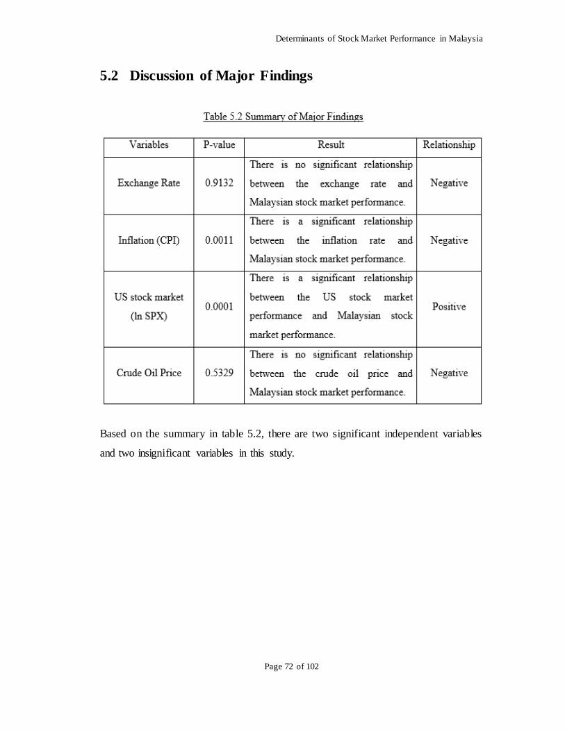
Determinants of Stock Market Performance in Malaysia
Page 72 of 102
5.2 Discussion of Major Findings
Based on the summary in table 5.2, there are two significant independent variables
and two insignificant variables in this study.
Determinants of Stock Market Performance in Malaysia
Page 73 of 102
5.2.1 Significant Variables
5.2.1.1 Inflation Rate
Table 5.2 shows that the inflation rate has a significant negative relationship with the
Malaysian stock market performance. Based on previous studies, it was a rare
situation to obtain a negative relationship between the inflation rate and stock market
performance. However, the result is consistent with the study of Chia and Lim (2015).
They found that the negative relationship was due to the unexpected changes in the
price level during inflation. The researchers claim that the announce ment of the
occurrence unanticipated of inflation helps in forecasting the future inflation level and
leads to decrease of the share price immediately. In theoretical basis, an unanticipated
inflation might cause the company facing liquidity problem due to high production
costs while the selling price of the product remains unchanged. In other words, it
leads to a shortage of fund in the operation of the company. Since the performances
and profits of the company are affected, a significant drop in the share price of those
companies will happen because investors expect the companies will unable to
perform well in the future.
Besides, Rahman et al. (2009) also stated that a negative relationship between the
inflation rate and stock market performance might be caused by the implementation
of the monetary policy. It could be supported by an article in Bloomberg which stated
that the government had focused on the implementation of the monetary policy that
highly related to inflation control in the past few years. Therefore, when the
government sold off the shares and bonds in a sudden during the year 2015, this had
directly affected the stock market performance in Malaysia
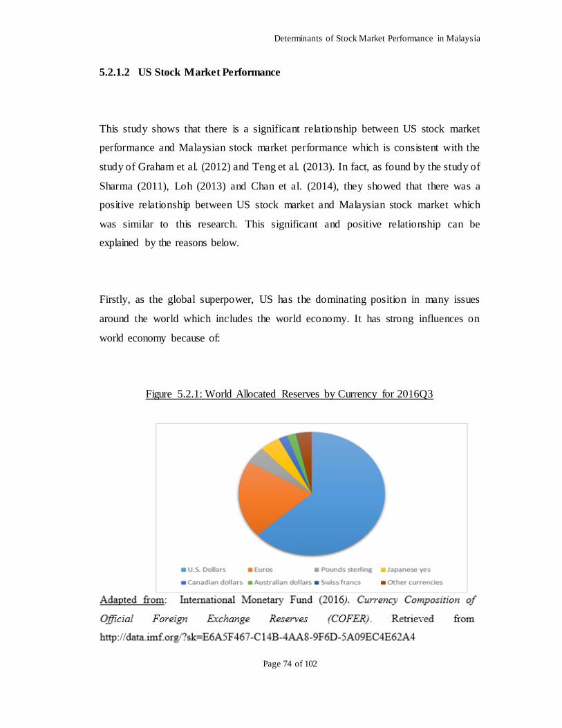
Determinants of Stock Market Performance in Malaysia
Page 74 of 102
5.2.1.2 US Stock Market Performance
This study shows that there is a significant relationship between US stock market
performance and Malaysian stock market performance which is consistent with the
study of Graham et al. (2012) and Teng et al. (2013). In fact, as found by the study of
Sharma (2011), Loh (2013) and Chan et al. (2014), they showed that there was a
positive relationship between US stock market and Malaysian stock market which
was similar to this research. This significant and positive relationship can be
explained by the reasons below.
Firstly, as the global superpower, US has the dominating position in many issues
around the world which includes the world economy. It has strong influences on
world economy because of:
Figure 5.2.1: World Allocated Reserves by Currency for 2016Q3
Determinants of Stock Market Performance in Malaysia
Page 75 of 102
US dollar is a key currency for international trade (Lee, 2013).
Most of the central bank and government in the world hold US dollar as their
main reserve currency (Lee, 2013). According to the Figure 5.2.1, more than
50% of U.S. dollar was allocated by the world as their reserves in 2016 Q3.
According to World Bank (2017), US contributed 24.32% which is the most
in world GDP during year 2015.
Since US is important to the world economy as shown by the facts above, any news,
either positive or negative that affecting US economy and its stock market, will
definitely weigh on the mind of the investors in other countries including Malaysia.
Therefore, when this kind of mindset and overreaction in stock market which
proposed by De Bondt and Thaler (1985) rooted in the investors, they could explain
the positive and significant relationship between Malaysian stock market and US
stock market.
In general, overreaction hypothesis stated that the stock price which acted like a
human behavior, would overreact to the good and bad news on stock market (Ali,
Nassir, Hassan and Abidin, 2010). The rationale behind this overreaction of stock
price is due to investors tend to overreact to new information released to them and
make decisions based on the latest information instead of the previous information
(De Bondt & Thaler, 1985).
In other words, investors might trade the stocks based on misconceptions derived
from the new information. Indeed, most of them are probably forgetting about the
share price of a company should price according to the company performance instead
of the new information received by them. This phenomena can be shown by the
reactions of investors towards the good news and bad news. The stock price will more

Determinants of Stock Market Performance in Malaysia
Page 76 of 102
than its fair value or true value when good news are released to the market.
Conversely, the stock price will below its fair value when investors receive the bad
news of a company.
However, the stock price would ultimately adjust to its fair value in long run, 3 to 5
years, because investors would take corrective actions after realizing their
overreaction behavior (De Bondt & Thaler, 1985). This situation was supported by
some more recent studies which was based on Malaysian context. According to Ali,
Ahmad and Anusakumar (2011), they found that stock overreaction had occurred in
Malaysian stock market for stock holdings more than 5 years. Interestingly, Ali,
Nassir, Hassan and Abidin (2011) discovered that economic events would trigger the
stock overreaction in Malaysian stock market. Therefore, using overreaction
hypothesis, as investors are concerned about US stock market due to its dominate
position in world economy, they tend to overreact and make harsh decisions when
any news that affect US disseminate to them. In other words, Malaysian investors
might react according to the trend of US stock market. If US stock market improves,
they will overreact by expecting Malaysian stock market will in an upward trend too.
In short, both stock markets have a positive relationship.
Determinants of Stock Market Performance in Malaysia
Page 77 of 102
5.2.2 Insignificant Variables
5.2.2.1 Exchange Rate
Some researchers found out that there was no significant relationship between
exchange rate and stock prices which was similar to the empirical result of this study.
For instance, those researchers are Solnik (1987), Chow, Lee and Solt (1997), Nieh
and Lee (2001), and Nguyen, Bui and Nguyen (2016).
According to Ooi, Wafa, Lajuni and Ghazali (2009), the asset market approach, at
other extreme, indicated there was no relationship at all between exchange rate and
stock prices. This was because the exchange rate was considered as one of the
important parts of an asset’s price in terms of foreign currency. Besides, the
researchers claimed that the main factors for the changes of current exchange rate and
the future exchange rate were not the same. For instance, the movement of exchange
rate might be affected by a country’s international trade performance. However, the
future exchange rate might be affected by major political and economic events such
as election, recession, war and change of government policy. Hence, no causal
relationship was existed between these two variables.
In addition, the result of Ooi et al. (2009) is aligned with Abidin, Walters, Lim and
Azilawati (2013) who stated that the insignificant long-run relationship between the
exchange rate and stock market prices could be influenced by not only the observed
financial factors, but also political factors such as government policy, expectation
Determinants of Stock Market Performance in Malaysia
Page 78 of 102
patterns and impact of election. These impacts could contribute to different predicting
power of stock market prices and exchange rates.
Interestingly, Ibrahim and Yusoff (2001) state that the movements of Malaysian stock
market are driven more by domestic factors rather than by the external factor such as
exchange rate. In general, it means that exchange rate as an external factor has less
significant impact to Malaysian stock market compared to those domestic factors. For
instance, the stock prices have immediate positive responses to the monetary
expansion. Increase in money supply will lead to an increase in the stock prices. In
another way, appreciation of exchange rate is positively related to money supply.
Hence, the stock price increases due to the increase of money supply. In brief, the
stock price is driven more by internal factors than the external factors.
5.2.2.2 Crude Oil Price
The crude oil price is found insignificantly related to the Malaysian stock market
performance in this study. In other words, the movement of crude oil price will not
affect the performance of the Malaysian stock market. The result is consistent with
various studies such as Murthy et al. (2017), Nordin et al. (2014) and Puah et al.
(2009). The insignificant result of crude oil price obtained might be due to the
government subsidization on the oil price in Malaysia. For instance, the government
will set the retail oil prices below the actual prices by providing subsidies, especially
when the crude oil price increases. In 2014, the government has provided RM 17.7
billion for the petroleum subsidies alone. Therefore, the subsidised price might
eliminate the impact of crude oil price movement to the stock price.
Determinants of Stock Market Performance in Malaysia
Page 79 of 102
5.3 Implications of the study
5.3.1 For the potential investors
Consideration of the macroeconomic factors is important for the investors before
entering the stock market. Hence, the knowledge and deep understanding of the
performance of the macroeconomics are a key success for the future investors. The
investors and stockholders will be more preferred to enter and hold their stocks when
there is a bull market while considering factors such as inflation rate and US stock
market performance at the same time. On the other hand, from the discussion on
major finding, it might help the potential investors and shareholders to determine the
relationship between the macroeconomic variables (inflation rate, exchange rate,
crude oil price and US stock market performance) and the Malaysian stock market
performance. Also, they might able to analyse and make a right decision by focusing
more on the significant variables.
Besides, the investors and shareholders might need to pay attentions on the monetary
policy implements by the government. As stated in the previous part, the monetary
policies would affect the internal monetary function of Malaysia such as the interest
rate and money supply. Moreover, it might also affect the stock market performance
indirectly. Hence, it is suggested for the investors and shareholders to be more alert of
the changes in monetary policies and analyse the impacts of the changes.
In addition, since US stock market is a relatively uncommon variable that introduced
in this research, the result of this research might help the potential investors to
Determinants of Stock Market Performance in Malaysia
Page 80 of 102
understand more about it. As shown by the result in this study, Malaysian stock
market performance has a positive and significant relationship with US stock market
performance. Undoubtedly, investors would be suggested to analyse US stock market
when constructing their portfolio investments in Malaysia. Nevertheless, due care
might be taken since there is a positive relationship between these two markets. First,
according to Markowitz (1991) who is known as the Father of Modern Portfolio
Theory, diversification in investment could reduce the uncertainty which was referred
as risks. However, portfolio diversification might not be appropriate since Malaysian
stock market and US stock market move in a same direction. This implies when
investors lose their investments in US stock market, the same incident will occur too
for their investments in the Malaysian stock market. Definitely, this is not the result
expects by diversification as the risks do no reduce in this case. In short, the positive
and significant relationship in the two stock markets indicates that Malaysia is not a
suitable country for portfolio diversification particularly for investors who hold stocks
in US market.
5.3.2 For the Government and Policy Makers
According to Janor et al. (2005), the researchers found that the stock market
performance could reflect the expectation of the future economy of Malaysia.
Furthermore, different stock market conditions will lead to the changes on economy
in Malaysia.
Indeed, the Malaysian government plays a vital role in influencing the factors that
affect the country. Hence, it is important for the government to have a clearer concept
on the relationship between the factors and the stock market performance. By
Determinants of Stock Market Performance in Malaysia
Page 81 of 102
referring to the results of this study, the government might have to analyse deeply
about the inflation rate and the US stock market performance since they are
significant to the stock market performance which eventually affect the country’s
economy.
Besides, insignificant variables do not indicate that they are irrelevant to the stock
market performance. In other words, they might represent a very limited effect to the
stock market performance in Malaysia. For instance, crude oil price is found to be
insignificant in this study. However, government has eliminated the subsidization in
recent year and will adjust the oil price monthly according to the changes of global oil
price. This implied the oil price volatility would eventually affect the stock market
performance in Malaysia. Hence, the government might need to consider the adverse
effect particularly the impact to the stock market after terminating the oil
subsidization policy. Besides, the policy makers might also need to take the
consequences into consideration when handling the government policy especially the
oil subsidy. This is to ensure the impact of oil price volatility to the stock prices will
be minimized.
For the policy makers, this study is important for them to identify shortcomings in the
policy implementation such as the monetary policy and make improvements. By
understanding this study, the policy makers might able to create the policy with the
consideration of several aspects instead of only focusing on the inflation problem.
Thus, with the cooperation of the policy makers and government, the stability of the
stock market can be achieved.
5.3.3 For the Future Researchers
Determinants of Stock Market Performance in Malaysia
Page 82 of 102
Refer to the literature review, there is a lot of argument on the topic of determinants
of the stock market performance which leads to different results. For example, Chia
and Lim (2015) and Kaur (2015) had concluded the relationship between the inflation
rate and stock market performance was in an opposite way. Nonetheless, this study
has provided the future researchers another prospective result by substituting the
common macroeconomic variables with the US stock market performance. Moreover,
this study provides future researchers a new model which is a combination of
selective variables such as the inflation rate, exchange rate, crude oil price and US
stock market. In other words, this study could be a guidance for future researchers
who study the determinants of the stock market performance.
5.4 Limitation
The limitations are very important for the development of the future research. They
allow the next researchers to investigate the issue in a more comprehensive way.
However, it is important to know that the limitations of this research are raised for the
further research purpose without distorting the finding of this research.
5.4.1 Restriction of Kuala Lumpur Composite Index (KLCI)
The Malaysian stock market performance is measured by using Kuala Lumpur
Composite Index (KLCI) in this study. In fact, many researches on this topic are
using KLCI as the indicator of Malaysian stock market performance. However, KLCI
is not the perfect indicator to examine all companies in the Malaysian stock market
Determinants of Stock Market Performance in Malaysia
Page 83 of 102
since KLCI only comprises the largest 30 companies by full market capitalization that
meet stated eligibility requirements (Rahman et al., 2009). Hence, the outcome of this
research may not be suitably applied to the other listed companies, especially for the
companies that are not included in the KLCI index. The potential users for the finding
of this research are required to be aware of this limitation.
5.4.2 Conversion Factor
As stated in Chapter 3, the data of CPI which is directly retrieved from the website of
Bank Negara Malaysia (BNM) involved two different base year which are 2005 and
2010. The overall study period is from 2009 to 2016, but the base year of the study
period for 2009 is based on 2005, while the base year of the study period from 2010
to 2016 is based on 2010. Thus, in order to make the data comparable, the 2005 based
year data has been converted into based year 2010 by using a conversion factor.
However, there is a limitation on the precision of the converted data of 2009 due to
the limited decimal places available. The data that showed on the website of BNM are
involved only two decimal points. Thus, it may violate the precision of the result by
using only two decimal places for the data conversion, but noted that the accuracy of
the result would not be affected (Sabo, 2003).
For illustration, Bertuzzi (2017) stated that the current world’s record in the 100-
meter dash is 9.58 seconds, but the actual time for the winner to finish the 100-meter
dash is 9.572 seconds, to be more precisely. He stated that there would be a difference
at the finish line between gold and silver if a third decimal place was encountered.
Determinants of Stock Market Performance in Malaysia
Page 84 of 102
Similarly, a lower decimal place used in the data conversion would affect its precision
level in obtaining the results.
5.4.3 Limited Resources
Limited resources in this research has caused the exclusion of selective independent
variables in the model such as money supply and interest rate. Both the excluded
independent variables are found significant to the Malaysian stock market
performance in prior studies. For example, Alzaid (2016) stated that the interest rate
and the money supply were significant to explain the Malaysian stock market
performance in a negative and positive manner respectively. Besides, these findings
are supported and proved by Asmy, Rohilina, Hassama and Fouad (2010) and
Rahman et al. (2009). However, due to limited resources, the study is prohibited from
further employing more independent variables in the model.
5.5 Recommendations for Future Research
Firstly, Kuala Lumpur Composite Index (KLCI) is not always the prefect indicator
for Malaysian Stock market performance because it only includes 30 listed companies.
Indeed, there are other Malaysia indexes which include Top 100 Index, EMAS Index,
Palm Oil Plantation Index, Hijrah Shariah Index and ACE Index. These indexes could
be used to measure the performance of the Malaysian stock market in different
sectors such as conventional, Shariah principles and palm oil plantation. The future
researcher could consider to use other indexes in order to better match their objectives.
Determinants of Stock Market Performance in Malaysia
Page 85 of 102
On the other hand, future researches are suggested to try different data frequency such
as in yearly, quarterly basis or weekly basis. This is because different independent
variables might have different sensitivity on a different frequency. For example, the
exchange rate may act more sensitive in daily data due to its high volatility. However,
there is always a challenge while collecting secondary data. In fact, numerous
researchers are always facing a problem and limitation while collecting data. Thus,
they might need to consider this limitation and overcome it when collecting the
secondary data.
Furthermore, future researchers are recommended to include more determinant in the
scope of research. They can consider qualitative variables such as current issues in
their study. For instance, the global stock markets are affected by uncertainties
created by the Brexit and election of US president recently but their relationships with
the stock market are yet to be studied. Besides, future researchers might examine the
relationship of the stock market performance in Malaysia with macroeconomic
variables of its neighbouring countries such as Singapore and Thailand by using a
more recent data. For example, from the evidence of the Asian Financial Crisis, there
might be a contagion effect between neighbouring countries.
Determinants of Stock Market Performance in Malaysia
Page 86 of 102
5.6 Conclusion
The main objective of this study is to investigate the relationship between the
selective variables and the Malaysian stock market performance. From the empirical
result, it showed that two variables were significant while the another two variables
were not. More specifically, there was an insignificant relationship between both
crude oil price and exchange rate to the Malaysian stock market performance. On the
other hand, the inflation rate and US stock market performance were having a
significant negative and positive relationship respectively with the Malaysian stock
market performance.
There was not much difficulty when performing the diagnostic checking. The only
problem faced in this study was the autocorrelation problem. Nevertheless, this
autocorrelation problem had been solved by using the Newey West (HAC) standard
error method.
While conducting this study, limitation on KLCI, conversion factor and limited
resources had hindered this study from providing a more comprehensive
understanding about the determinants of Malaysian stock market performance. Hence,
the recommendation section of this study had drawn some suggestions which might
be helpful for the future researchers of this relevant study.
Lastly, this research provided an opportunity for the members of this research to
practice on the techniques and knowledge acquired previously in the classroom.
Besides, the members were also able to obtain a deeper understanding about the
relationship of selective variables with the Malaysian stock market performance by
carrying out the literature review and the data collection. Also, it was a good learning
experience for the degree students to communicate effectively and work with others
as a preparation for their future career paths.
Determinants of Stock Market Performance in Malaysia
Page 87 of 102
REFERENCES
Abidin, S., Walters, C., Lim, K. L., & Azilawati, B. (2013). Cointegration between
stock prices and exchange rates in Asia-Pacific countries. Investment Management and Financial Innovations, 10(2), 142-146
Adeboye, N. O., Fagoyinbo, I. S., & Olatayo, T. O. (2014). Estimation of the effect of
multicollinearity on the standard error for regression coefficients. Journal of
Mathematics, 10(4), 16-20.
Akinwande, M. O., Dikko, H. G., & Samson, A. (2015). Variance Inflation Factor: As a condition for the inclusion of suppressor variable(s) in regression analysis. Open Journal of Statistics, 5, 754-767.
Ali, N., Nassir, A. M., Hassan, T., & Abidin, S. Z. (2010). Short Run Stock
Overreaction: Evidence from Bursa Malaysia. International Journal of Economics and Management, 4(2), 319-333.
Ali, N., Nassir, A. M., Hassan, T., & Abidin, S. Z. (2011). Stock Overreaction Behaviour in Bursa Malaysia: Does the Length of the Formation Period Matter?.
British Journal of Economics, Finance and Management Sciences, 2(2), 319–333.
Ali, R., Ahmad, Z. & Anusakumar, S. V. (2011). Stock Market Overreaction and Trading Volume: Evidence from Malaysia. ASIAN Academy of Management
Journal of Accounting and Finance, 7(2), 103-119. Allen, F. & Carletti, E. (2010). An Overview of the Crisis: Causes, Consequences,
and Solutions. International Review of Finance, 10(1), 1-26.
Almunia, M., Bénétrix, A. S., Eichengreen, B., O’Rourke, K. H. & Rua, G (2010). From Great Depression to great credit crisis: Similarities, differences and lessons. Economic Policy, 25(62), 219–265.
Aloui, C., Nguyen, D. K. & Njeh, H. (2012). Assessing the impacts of oil price
fluctuations on stock returns in emerging markets. Economic Modelling, 29(6), 2686-2695.
Alzaid, S. (2016). The Kuala Lumpur Stock Exchange Composite Index (KLSE CI) and economic forces. South East Asia Journal of Contemporary Business,
Economics and Law, 10(3), 53-64. Andale. (2016). Jarque-Bera Test. Retrieved from
http://www.statisticshowto.com/jarque-bera-test/
Determinants of Stock Market Performance in Malaysia
Page 88 of 102
Apergis, N., & Miller, S. M. (2009). Do structural oil-market shocks affect stock prices?. Energy Economics, 31(4), 569-575.
Arouri, M., Dar, A. B., Bhanja, N., Tiwari, A. K. & Teulon, F. (2015). Stock Return
and Inflation in Pakistan. Economic Modeling, 47, 23-31. Arshad, M. N. & Yahya, M. H. (2016). Relationship between Stock Market Returns
and Exchange rates In Emerging Stock Markets. Journal of Islamic Economics and Business, 1(2), 131-143.
Asayesh, H. & Gharavi, M. Z. (2015). The Impact of Inflation on Stock Price with
Panel Data (Case Study: Tehran Stock Exchange). International Journal of
Administration and Governance, 1(9), 6-11.
Asmy, M., Rohilina, W., Hassama, A. & Fouad, M. (2010). Effects of macroeconomic variables on stock prices in Malaysia: An approach of error correction model. (MPRA Paper No. 20970). Retrieved from https://mpra.ub.uni-
muenchen.de/20970/1/MPRA_paper_20970.pdf
Australian Bureau of Statistics. (2012a). Re-referencing and Linking Price Indexes. Retrieved from http://www.abs.gov.au/ausstats/[email protected]/Previousproducts/6461.0Main%20Fea
tures132009?opendocument&tabname=Summary&prodno=6461.0&issue=2009&num=&view=
Australian Bureau of Statistics. (2012b). Re-referencing Frequently Asked Questions.
Retrieved from
http://www.abs.gov.au/ausstats/[email protected]/Previousproducts/6401.0Main%20Features8Sep%202012?opendocument&tabname=Summary&prodno=6401.0&issu
e=Sep%202012&num=&view= Azizan, N. A., & Sulong, H. (2011). The Preparation towards Asean Exchange Link
between Malaysia Stock Market and Asia Countries Macroeconomics Variables Interdependency. International Journal of Business and Social Science, 2(5),
128-134. Bai, Z. (2014). Study on the Impact of Inflation on the Stock Market in China.
International Journal of Business and Social Science, 5(7), 261-271.
Bertuzzi, S. (2017). A false sense of precision. Retrieved from http://www.ascb.org/activation-energy/a-false-sense-of-precision-what-happens-to-journal- impact-factor-jif-rankings-when-you-drop-a-decimal-place/
Bloomberg, L. P. (2017). Historical Data for FBMKLCI Index 03/01/1977 to
12/31/2016. Retrieved from Bloomberg database.
Determinants of Stock Market Performance in Malaysia
Page 89 of 102
Bordo, M., & James, H. (2010). The Great Depression analogy. Financial History Review, 17(02), 127-140.
Boubaker, H. & Sghaier, N. (2014). Instability and dependence structure between oil
prices and GCC stock markets. Energy Studies Review, 20(3), 50-65. Chan, S. G., Karim, M. Z., & Karim, M. Z. (2010). Volatility Spillovers of the Major
Stock Markets in ASEAN-5 with U.S. and Japanese Stock Markets. International Research Journal of Finance and Economics, 44, 157-168.
Chari, V. V. & Christiano, L. (2014). The optimal extraction of exhaustible resources.
Economic Policy Paper, 14(5), 1-7.
Chen, N. F., Roll, R., & Ross, S. A. (1986). Economic forces and the stock market.
The Journal of Business, 59(3), 383-403. Chia, R. C. J. & Lim, S. Y. (2015). Malaysia Stock Price And Macroeconomic
Variables: Autoregressive Distributed Lag (ARDL) Bounds Test. Kajian Malaysia. 33, 85-103.
Chkili, W., & Nguyen, D. K. (2014). Exchange Rate Movements and Stock Market
Returns in a Regime-switching Environment: Evidence for BRICS Countries.
Research in International Business and Finance, 31, 46-46.
Chow, E. H., Lee, W. Y., & Solt, M. S. (1997). The exchange rate risk exposure of asset returns. Journal of Business, 70, 105-123.
Cohen, J., Cohen, P., West, S. G., & Aiken, L. S. (2003). Applied multiple regression/correlation analysis for the behavioral sciences (3rd ed.). Mahwah,
NJ: Lawrence Erlbaum Associates. Conrad, C. F. & Serlin, R. C. (2011). The SAGE Handbook for Research in Education:
Pursing Ideas as the Keystone of Exemplary Inquiry (2nd ed.). London, United Kingdom: SAGE Publications.
Corradi, V., Distaso, W., & Mele, A. (2013). Macroeconomic determinants of stock
volatility and volatility premiums. Journal of Monetary Economics, 60(2), 203-
220.
De Bondt, W. F. M. & Thaler, R. H. (1985). Does the Stock Market Overreact? Journal of Finance, 40(3), 42-56.
Dhaoui, A. & Khraief, N. (2014). Empirical linkage between oil price and stock market returns and volatility: Evidence from international developed markets.
Economics, 12, 1-30.
Determinants of Stock Market Performance in Malaysia
Page 90 of 102
Dimitrova, D. (2005). The relationship between exchange rates and stock prices: Studied in a multivariate model. Issues in Political Economy, 14(1), 3-9.
Fisher, I. (1930). The theory of interest. New York, United States: MacMillan.
Gale, D. (1955). The law of supply and demand. Mathematica Scandinavica, 3, 155-
169.
Graham, M., Kiviaho, J., & Nikkinen, J. (2012). Integration of 22 emerging stock
markets: A three-dimensional analysis. Global Finance Journal, 23(1), 34-47. Greene, W. H. (2003). Econometric analysis. New Jersey, United States: Pearson
Education LTD.
Gujarati, D. N., & Porter, D. C. (2009). Basic Econometrics (5th ed.). USA: McGraw-Hill.
Hadi, A. R. R., Yahya, M. H., & Shaari, A. H. (2009). The effect of oil price fluctuations on the Malaysian and Indonesian Stock Markets. Asian Journal of
Business and Accounting, 2(1&2), 69-91. Hamilton, J. D. (2008). Understanding crude oil prices. The Energy Journal,
International Association for Energy Economics, 30(2), 179-206.
Hotelling, H. (1931). The economics of exhaustible resources. The Journal of Political Economy, 39(2), 137-175.
Hutcheson, G. D., & Moutinho, L. (2011). The SAGE dictionary of quantitative
management research. London, United Kingdom: SAGE Publications Ltd. Hutcheson, G. D., & Sofroniou, N. (1999). The multivariate social scientist. London,
United Kingdom: SAGE Publications Ltd.
Ibrahim, M. H. (2006). Integration or Segmentation of the Malaysian Equity Market: An Analysis of Pre- and Post-Capital Controls. Journal of the Asia Pacific Economy, 11(4), 424-443.
Ibrahim, M. H., & Yusoff, W. S. W. (2001). Macroeconomic variables, exchange rate
and stock price: A Malaysian Perspective. Journal of Economics and Management 9, 2, 141-63.
Imarhiagbe, S. (2010). Impact of oil prices on stock markets: Empirical evidence from selected major oil producing and consuming countries. Global Journal of
Finance and Banking Issues, 4(4), 15-31.
Determinants of Stock Market Performance in Malaysia
Page 91 of 102
International Monetary Fund. (2016). Currency Composition of Official Foreign Exchange Reserves (COFER). Retrieved from
http://data.imf.org/?sk=E6A5F467-C14B-4AA8-9F6D-5A09EC4E62A4
James, H. (2010). 1929: The New York Stock Market Crash. Representations, 110(1), 129-144.
Janor, H., Halid, N., & Rahman, A. A. (2005). Stock Market and Economic Activity in Malaysia. Journal of Investment Management and Financial Innovation, 4,
116-123. Jareño, F. & Negrut, R. (2016). US Stock Market and Macroeconomic Factors.
Journal of Applied Business Research, 32(1), 325-340.
Jarque, C. M., & Bera, A. K. (1987). A test for normality of observations and regression residuals. International Statistical Review, 55, 163–172.
Jarvis, C. B., Mackenzie, S. B., & Podsakoff, P. M. (2003). A Critical Review of Construct Indicators and Measurement Model Misspecification in Marketing
and Consumer Research. Journal of Consumer Research, 30, 199-218. Jeffrey, D. C., James, J. C., Michael, J. F., Jeffrey, W. O. & David, R. A. (2015).
Essentials of business analytics. Stamford, CT: Cengage Learning.
Kadochnikov, D. V. (2013). Gustav Cassel’s Purchasing Power Parity Doctrine in the context of his views on International Economic Policy Coordination. Euro. J. History of Economic Thought, 20(6), 1101-1121.
Kang, W., Ratti, R. A. & Vespignani, J. (2016). The impact of oil price shocks on the
US stock market: A note on the roles of US and non-US oil production. Economics Letters, 145, 176-181.
Kandil, M., Berument, H. & Dincer, N. N. (2007). The effects of exchange rate fluctuations on economic activity in Turkey. Journal of Asian Economics, 18,
466-489. Katechos, G. (2011). On the Relationship between Exchange Rates and Equity
Returns: A New Approach. Journal of International Financial Markets, Institutions & Money, 21(4), 550-559.
Kaur, H. (2015). A Study of Impact of Inflation on National Stock Index.
International Journal of Advanced Research in Management and Social Science,
4(7), 95-99.
Khan, T. A. (2011). Cointegration of International Stock Markets: An Investigation of Diversification Opportunities. Undergraduate Economic Review, 8(1), 1-50.
Determinants of Stock Market Performance in Malaysia
Page 92 of 102
Kibria, U., Mehmood, Y., Kamran, M., Arshad, M. U., Perveen, R., & Sajid, M.
(2014). The Impact of Macroeconomc Variables on Stock Market Returns: A Case of Pakistan. Research Journal of Management Sciences, 3(8), 1-7.
Kimani, D. K., & Mutuku, C. (2013). Inflation dynamics on the overall stock market
performance: The case of Nairobi securities exchange in Kenya. Journal of
Economics and Finance Review, 2(11), 1-11.
Kupchan, C. A. (2012). The Democratic Malaise: Globalization and the Threat to the West. Foreign Affairs, 91(1), 62-67.
Kuwornu, J. K. M. & Owusu – Nantwi, V. (2011). Macroeconomic variables and stock market returns: Full information maximum likelihood estimation.
Research Journal in Finance and Accounting, 2(4), 49-63. Lamont, O. A., & Thaler, R. H. (2003). The Law of One Price in Financial Markets.
Journal of Economic Perspectives, 17(4), 191-202.
Lee, J. W. (2013). Will the Renminbi Emerge as an International Reserve Currency?. The World Economy, 37(1), 42-62.
Levine, R., & Zervos, S. (1998). Stock markets, banks, and economic growth. American economic review, 88(3), 537-558.
Lim, C. M., & Sek, S. K. (2014). Modelling the Dynamic Relationship between U.S.’
and Malaysia’s Stock Market Volatility. International Journal of Trade,
Economics and Finance, 5(1), 43-47.
Liu, L., & Wan, J. (2012). The Relationships between Shanghai Stock Market and CNY/USD Exchange Rate: New Evidence based on Cross-correlation Analysis, Structural Cointegration and Nonlinear Causality Test. Physica A: Statistical
Mechanics and its Applications, 391(23), 6051-6059.
Loh, L. (2013). Co-movement of Asia-Pacific with European and US stock market returns: A cross-time-frequency analysis. Research in International Business and Finance, 29, 1-13.
Markowitz, H. M. (1991). Foundations of portfolio theory. The Journal of Finance,
46(2), 469-477. Martin, A. & Ventura, J. (2012). Economic Growth with Bubbles. The American
Economic Review, 102(6), 3033-3058
Determinants of Stock Market Performance in Malaysia
Page 93 of 102
Mbulawa, S. (2015). The Impact of Inflation on Stock Market Performance Zimbanwe between 1980 and 2008: An Empirical Study Investigation.
European Journal of Business, Economics and Accounting, 3(4), 62-70.
Miller, J. I., & Ratti, R. A. (2009). Crude oil and stock markets: Stability, instability, and bubbles. Energy Economics, 31(4), 559-568.
Minnitt, R. C. A. (2007). Frontiers of usefulness: The economics of exhaustible resources. The Journal of the Southern African Institute of Mining and
Metallurgy, 107(8), 539-555. Moore, T., & Wang, P. (2014). Dynamic Linkage between Real Exchange Rates and
Stock Prices: Evidence from Developed and Emerging Asian Markets. International Review of Economics and Finance, 29, 1-11.
Murthy, U., Anthony, R., & Vighneswaran, R. (2017). Factors affecting Kuala
Lumpur Composite Index (KLCI) stock market return in Malaysia.
International Journal of Business and Management, 12(1), 122-132.
Mutuku, C., & Ng’eny, K. L. (2015). Macroeconomic Variables and the Kenyan Equity Market: A Time Series Analysis. Business and Economic Research, 5(1), 1-10.
Nandha, M. & Hammoudeh, S. (2007). Systematic risk, and oil price and exchange
rate sensitivities in Asia-Pacific stock markets. International Business and Finance, 21(2), 326-341.
Nguyen, H. (2010). Examining the relationship between crude oil returns and emerging stock markets in Asia. Retrieved from
http://dare.uva.nl/cgi/arno/show.cgi?fid=215292 Nguyen, T. D., Bui, Q. H., & Nguyen, T. T. (2016). Causal Correlation between
Exchange Rate and Stock Index: Evidence from VN-Index. Asian Social Science, 12(8), 43-55.
Nieh, C. C., & Lee, C. F. (2001). Dynamic relationship between stock prices and
exchange rates for G-7 countries. The Quarterly Review of Economics and
Finance, 41, 477-490.
Nordin, N., Nordin, S. & Ismail, R. (2014). The impact of commodity prices, interest rate and exchange rate on stock market performance: An empirical analysis from Malaysia. Malaysian Management Journal, 18, 39-52.
Omotor, D. G. (2010). Relationship between inflation and stock market returns:
Evidence from Nigeria. Journal of Applied Statistics, 1(1), 1-15.
Determinants of Stock Market Performance in Malaysia
Page 94 of 102
Ono, S. (2011). Oil price shocks and stock markets in BRICs. The European Journal of Comparative Economics, 8(1), 29-45.
Ooi, A. Y., Wafa, S. A. W. S. K., Lajuni, N., & Ghazali, M. F. (2009). Causality
between Exchange Rates and Stock Prices: Evidence from Malaysia and Thailand. International Journal of Business and Management, 4(3), 86-98.
Oprea, D. S. (2014). The fisher effect: Evidence from the Romanian Stock Market. International Journal of Academic Research in Business and Social Sciences,
4(5), 637-644. Ouma, W. N., & Muriu, P. (2014). The Impact of Macroeconomic Variables on Stock
Market Returns in Kenya. International Journal of Business and Commerce, 3(11), 1-31.
Palamalai, S., Kalaivani, M., & Devakumar, C. (2013). Stock Market Linkages in
Emerging Asia-Pacific Markets. SAGE Open, 3(4), 1-15.
Paul, R. K. (2014). Multicollinearity: Causes, effects and remedies. Journal of IASRI,
New Delhi, 1-14. Payne, N. (2014). Evaluating the impact of heteroscedasticity on the predictive ability
of modern regression techniques (Master’s thesis). Simon Fraser University, British Columbia, Canada.
Plíhal, T. (2016). Stock Market Informational Efficiency in Germany: Granger
Causality between DAX and Selected Macroeconomic Indicators. Journal of
Social and Behavioral Science, 220, 321-329.
Puah, C. H., Tan, L. P. & Isa, A. H. M. (2009). Nexus between oil price and stock performance of power industry in Malaysia (MPRA Paper No. 31757). Retrieved from https://mpra.ub.uni-
muenchen.de/31757/1/MPRA_paper_31757.pdf
Rahman, A. A., Sidek, N. Z. M. & Tafri, F. H. (2009). Macroeconomic determinants of Malaysian stock market. African Journal of Business Management, 3(3), 95-106.
Ralph, J., O’Neill, R., & Winton, J. (2015). A Practical Introduction to Index
Numbers. [e-book]. Retrieved from https://books.google.com.my/books?id=wEb3CQAAQBAJ&pg=PT134&lpg=PT134&dq=re-
reference+cpi&source=bl&ots=KiYsyVT6d_&sig=tUVilGAu3gvAG_mEB3siK4PKazY&hl=en&sa=X&redir_esc=y#v=onepage&q=re-
reference%20cpi&f=false
Determinants of Stock Market Performance in Malaysia
Page 95 of 102
Ramadan, I. Z. (2012). The validity of the Arbitrage Pricing Theory in Jordanian Stock Market. International Journal of Economics and Finance, 4(5), 177-185.
Reboredo, J. C., Rivera, C. M. A., & Ugolini, A. (2016). Downside and Upside Risk
Spillovers between Exchange Rates and Stock Prices. Journal of Banking & Finance, 62, 76-96.
Ross, S. A. (1976). The Arbitrage Theory of Capital Asset Pricing. Journal of Economic Theory, 13, 341-360.
Sabo, D. W. (2003). Accuracy, Precision, and Significant Digits. Retrieved from
http://commons.bcit.ca/math/competency_testing/testinfo/testsyll11/approxnum
/accandprec/accandprec.pdf
Salamudin, N., Bakar, R., Ibrahim, M. K. & Hassan, F. H. (2010). Intangible assets valuation in the Malaysian capital market. Journal of Intellectual Capital, 11(3), 391-405.
Sarno, L., & Taylor, M. P. (2002). Purchasing Power Parity and the Real Exchange
Rate. IMF Staff Papers, 49(1), 65-105. Schenk, C. R. (2013). The dissolution of a monetary union: the case of Malaysia and
Singapore 1963-1974. Journal of Imperial and Commonwealth History, 41(3), 496-522.
Shaikh, A. (2011). The First Great Depression of the 21st Century. Socialist Register,
47(47), 44-63.
Sharma, P. (2011). ASIAN emerging economies and United States of America: Do
they offer a diversification benefit?. Australian Journal of Business and Management Research, 1(4), 85-92.
Shimizu, C., Karato, K. & Asami, Y. (2010). Estimation of redevelopment probability using panel data: Asset bubble burst and office market in Tokyo. Journal of
Property Investment & Finance, 28(4), 285-300. Siddiqui, M. M. (2014). Oil price fluctuation and stock market performance – The
case of Pakistan. Journal of International Business and Economics, 2(1), 47-53.
Solnik, B. (1987). Using financial prices to test exchange rate models: A note. Journal of Finance, 42, 141-149.
Srinivasan, P. (2011). Causal Nexus between Stock Market Return and Selected Macroeconomic Variables in India: Evidence from the National Stock
Exchange (NSE). IUP Journal of Financial Risk Management, 8(4), 7-24.
Determinants of Stock Market Performance in Malaysia
Page 96 of 102
Subramanian, M. (2015). A Study on Impact of Macroeconomic variables In the Stock Market. International Journal of Economics and Management Study,
2(5), 25-33.
Teng, K. T., Yen, S. H., & Chua, S. Y. (2013). Synchronization of stock market cycles: The importance of emerging and developed markets to ASEAN-5. Pague Economic Papers, 4, 435-458.
Tsai, I. C. (2012). The Relationship between Stock Price Index and Exchange Rate in
Asian Markets: A Quantile Regression Approach. Journal of International Financial Markets, Institutions & Money, 22(3), 609-621.
Tudor, C., & Popescu, D. C. (2012). On the Causal Relationship between Stock Returns and Exchange Rates Changes for 13 Developed and Emerging Markets.
Social and Behavioral Sciences, 57, 275-282. Tuyon, J. & Ahmad, Z. (2016). Behavioral finance perspectives on Malaysian stock
market efficiency. Borsa Istanbul Review, 16(1), 43-61.
Uddin, S. S. & Ahsan, L. (2014). Impact of Asian Financial Crisis in Malaysian Economy with special reference to Multinational Companies. Research Journal of Management Sciences, 3(9), 7-12.
Umar, Z. & Spierdijk L. (2015). Stocks, bonds, T-bills and inflation hedging: From
great moderation to great recession. Journal of Economics and Business, 79, 1-37.
United States Census Bureau. (2012). Construction Price Indexes. Retrieved from https://www.census.gov/construction/cpi/faqs/newpriceindexqa.html
Uwubanmwen, A. & Eghosa, I. L. (2015). Inflation Rate and Stock Return: Evidence
from the Nigerian Stock Market. International Journal of Business and Social
Science, 6(11), 155-167.
Vatcheva, K. P., Lee, M. J., McCormick, J. B., & Rahbar, M. H. (2016). Multicollinearity in regression analyses conducted in epidemiologic studies. Epidemio, 6(2), 1-9.
Williams, R. (2015). Heteroskedasticity. Retrieved from
https://www3.nd.edu/~rwilliam/stats2/l25.pdf Wong, B. (2014). Introduction to (generalized) autoregressive conditional
heteroskedasticity models in time series (Honors thesis). University of Washington, Washington, United States.
Determinants of Stock Market Performance in Malaysia
Page 97 of 102
Wooldridge, J. M. (2005). Introductory econometrics: A modern approach (3rd ed.). Mason, OH: South-Western College Publishing.
Wooldridge, J. M. (2013). Introductory econometrics: A modern approach (5th ed.).
Manson, OH: South-Western. World Bank (2017). Gross domestic product 2015. Retrieved from
http://databank.worldbank.org/data/download/GDP.pdf
Yeoh, B. K., Hooy, C. W. & Arsad, Z. (2010). Time- Varying World Integration of the Malaysian Stock Market: A Kalman Filter Approach. Asian Academy of Management Journal of Accounting and Finance, 6(2), 1-17
Yu, H., Jiang, S., & Land, K .C. (2015). Multicollinearity in hierarchical linear
models. Social Science Research, 53, 118-136. Zhang, C. (2013). Money, housing, and inflation in China. Journal of Policy
Modeling, 35(1), 75-87.
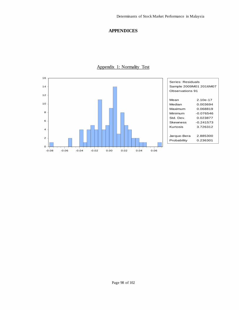
Determinants of Stock Market Performance in Malaysia
Page 98 of 102
APPENDICES
Appendix 1: Normality Test
0
2
4
6
8
10
12
14
16
-0.08 -0.06 -0.04 -0.02 0.00 0.02 0.04 0.06
Series: Residuals
Sample 2009M01 2016M07
Observations 91
Mean 2.10e-17
Median 0.003694
Maximum 0.068819
Minimum -0.076546
Std. Dev. 0.023877
Skewness -0.241573
Kurtosis 3.726312
Jarque-Bera 2.885300
Probability 0.236301
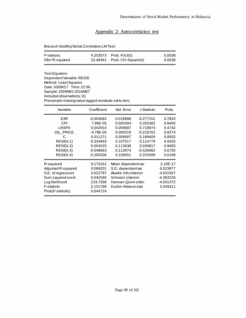
Determinants of Stock Market Performance in Malaysia
Page 99 of 102
Appendix 2: Autocorrelation test
Breusch-Godfrey Serial Correlation LM Test: F-statistic 4.203573 Prob. F(4,82) 0.0038
Obs*R-squared 15.48461 Prob. Chi-Square(4) 0.0038
Test Equation:
Dependent Variable: RESID
Method: Least Squares
Date: 03/08/17 Time: 22:36
Sample: 2009M01 2016M07
Included observations: 91
Presample missing value lagged residuals set to zero. Variable Coefficient Std. Error t-Statistic Prob. EXR -0.004683 0.016898 -0.277151 0.7824
CPI 7.98E-05 0.000394 0.202482 0.8400
LNSPX 0.042914 0.059687 0.718974 0.4742
OIL_PRICE -4.78E-05 0.000219 -0.218762 0.8274
C 0.011271 0.059507 0.189409 0.8502
RESID(-1) -0.334893 0.107517 -3.114779 0.0025
RESID(-2) 0.004525 0.113638 0.039817 0.9683
RESID(-3) -0.048663 0.113974 -0.426962 0.6705
RESID(-4) -0.260336 0.109551 -2.376399 0.0198 R-squared 0.170161 Mean dependent var 2.10E-17
Adjusted R-squared 0.089201 S.D. dependent var 0.023877
S.E. of regression 0.022787 Akaike info criterion -4.631557
Sum squared resid 0.042580 Schwarz criterion -4.383230
Log likelihood 219.7358 Hannan-Quinn criter. -4.531372
F-statistic 2.101786 Durbin-Watson stat 2.049311
Prob(F-statistic) 0.044724
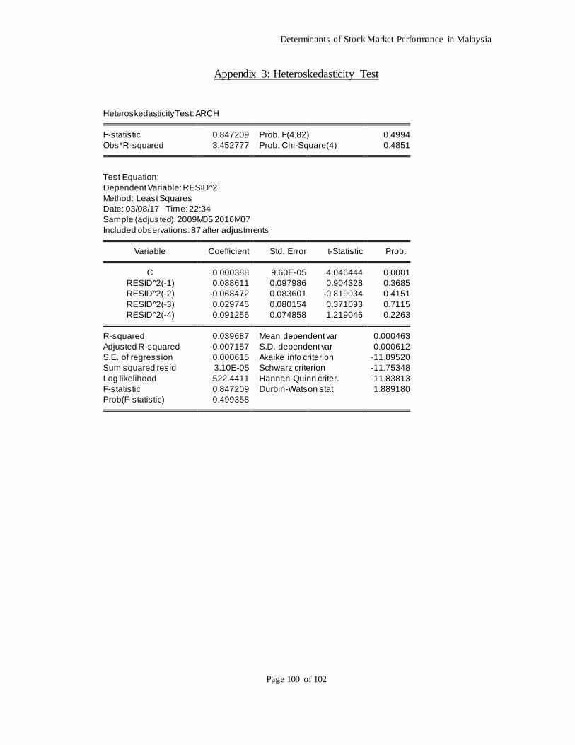
Determinants of Stock Market Performance in Malaysia
Page 100 of 102
Appendix 3: Heteroskedasticity Test
Heteroskedasticity Test: ARCH F-statistic 0.847209 Prob. F(4,82) 0.4994
Obs*R-squared 3.452777 Prob. Chi-Square(4) 0.4851
Test Equation:
Dependent Variable: RESID^2
Method: Least Squares
Date: 03/08/17 Time: 22:34
Sample (adjusted): 2009M05 2016M07
Included observations: 87 after adjustments Variable Coefficient Std. Error t-Statistic Prob. C 0.000388 9.60E-05 4.046444 0.0001
RESID^2(-1) 0.088611 0.097986 0.904328 0.3685
RESID^2(-2) -0.068472 0.083601 -0.819034 0.4151
RESID^2(-3) 0.029745 0.080154 0.371093 0.7115
RESID^2(-4) 0.091256 0.074858 1.219046 0.2263 R-squared 0.039687 Mean dependent var 0.000463
Adjusted R-squared -0.007157 S.D. dependent var 0.000612
S.E. of regression 0.000615 Akaike info criterion -11.89520
Sum squared resid 3.10E-05 Schwarz criterion -11.75348
Log likelihood 522.4411 Hannan-Quinn criter. -11.83813
F-statistic 0.847209 Durbin-Watson stat 1.889180
Prob(F-statistic) 0.499358
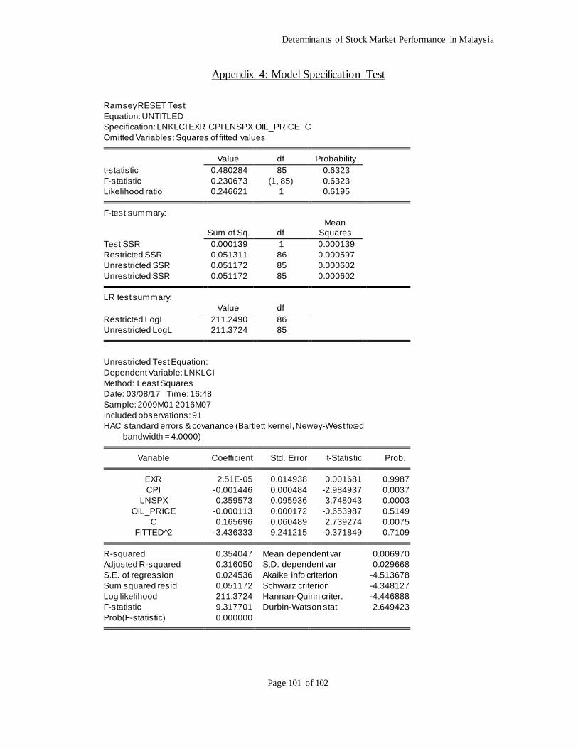
Determinants of Stock Market Performance in Malaysia
Page 101 of 102
Appendix 4: Model Specification Test
Ramsey RESET Test
Equation: UNTITLED
Specification: LNKLCI EXR CPI LNSPX OIL_PRICE C
Omitted Variables: Squares of fitted values Value df Probability
t-statistic 0.480284 85 0.6323
F-statistic 0.230673 (1, 85) 0.6323
Likelihood ratio 0.246621 1 0.6195 F-test summary:
Sum of Sq. df Mean
Squares
Test SSR 0.000139 1 0.000139
Restricted SSR 0.051311 86 0.000597
Unrestricted SSR 0.051172 85 0.000602
Unrestricted SSR 0.051172 85 0.000602 LR test summary:
Value df
Restricted LogL 211.2490 86
Unrestricted LogL 211.3724 85
Unrestricted Test Equation:
Dependent Variable: LNKLCI
Method: Least Squares
Date: 03/08/17 Time: 16:48
Sample: 2009M01 2016M07
Included observations: 91
HAC standard errors & covariance (Bartlett kernel, Newey-West fixed
bandwidth = 4.0000) Variable Coefficient Std. Error t-Statistic Prob. EXR 2.51E-05 0.014938 0.001681 0.9987
CPI -0.001446 0.000484 -2.984937 0.0037
LNSPX 0.359573 0.095936 3.748043 0.0003
OIL_PRICE -0.000113 0.000172 -0.653987 0.5149
C 0.165696 0.060489 2.739274 0.0075
FITTED^2 -3.436333 9.241215 -0.371849 0.7109 R-squared 0.354047 Mean dependent var 0.006970
Adjusted R-squared 0.316050 S.D. dependent var 0.029668
S.E. of regression 0.024536 Akaike info criterion -4.513678
Sum squared resid 0.051172 Schwarz criterion -4.348127
Log likelihood 211.3724 Hannan-Quinn criter. -4.446888
F-statistic 9.317701 Durbin-Watson stat 2.649423
Prob(F-statistic) 0.000000
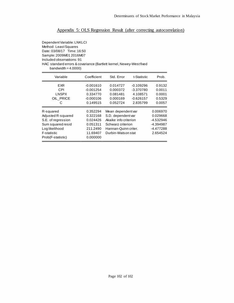
Determinants of Stock Market Performance in Malaysia
Page 102 of 102
Appendix 5: OLS Regression Result (after correcting autocorrelation)
Dependent Variable: LNKLCI
Method: Least Squares
Date: 03/08/17 Time: 16:50
Sample: 2009M01 2016M07
Included observations: 91
HAC standard errors & covariance (Bartlett kernel, Newey-West fixed
bandwidth = 4.0000) Variable Coefficient Std. Error t-Statistic Prob. EXR -0.001610 0.014727 -0.109296 0.9132
CPI -0.001254 0.000372 -3.370780 0.0011
LNSPX 0.334770 0.081481 4.108571 0.0001
OIL_PRICE -0.000106 0.000169 -0.626157 0.5329
C 0.149515 0.052724 2.835799 0.0057 R-squared 0.352294 Mean dependent var 0.006970
Adjusted R-squared 0.322168 S.D. dependent var 0.029668
S.E. of regression 0.024426 Akaike info criterion -4.532946
Sum squared resid 0.051311 Schwarz criterion -4.394987
Log likelihood 211.2490 Hannan-Quinn criter. -4.477288
F-statistic 11.69407 Durbin-Watson stat 2.654524
Prob(F-statistic) 0.000000