determination and interpretation of characteristic … · iaea/aq/48 iaea analytical quality in...

IAEA/AQ/48

IAEA Analytical Quality in Nuclear Applications Series No. 48

Determination and Interpretation of Characteristic Limits for Radioactivity Measurements

INTERNATIONAL ATOMIC ENERGY AGENCYVIENNA

ISSN 2074–7659

Determ

ination and Interpretation of Characteristic Lim

its for Radioactivity M

easurements

Decision Threshold, Detection Limit and Limits of the Confidence Interval

Template has: 20 mm spineplease reset it to the corrected spine/

DETERMINATION AND INTERPRETATION OF CHARACTERISTIC LIMITS

FOR RADIOACTIVITY MEASUREMENTS

AFGHANISTANALBANIAALGERIAANGOLAANTIGUA AND BARBUDAARGENTINAARMENIAAUSTRALIAAUSTRIAAZERBAIJANBAHAMASBAHRAINBANGLADESHBARBADOSBELARUSBELGIUMBELIZEBENINBOLIVIA, PLURINATIONAL

STATE OFBOSNIA AND HERZEGOVINABOTSWANABRAZILBRUNEI DARUSSALAMBULGARIABURKINA FASOBURUNDICAMBODIACAMEROONCANADACENTRAL AFRICAN

REPUBLICCHADCHILECHINACOLOMBIACONGOCOSTA RICACÔTE D’IVOIRECROATIACUBACYPRUSCZECH REPUBLICDEMOCRATIC REPUBLIC

OF THE CONGODENMARKDJIBOUTIDOMINICADOMINICAN REPUBLICECUADOREGYPTEL SALVADORERITREAESTONIAETHIOPIAFIJIFINLANDFRANCEGABON

GEORGIAGERMANYGHANAGREECEGUATEMALAGUYANAHAITIHOLY SEEHONDURASHUNGARYICELANDINDIAINDONESIAIRAN, ISLAMIC REPUBLIC OF IRAQIRELANDISRAELITALYJAMAICAJAPANJORDANKAZAKHSTANKENYAKOREA, REPUBLIC OFKUWAITKYRGYZSTANLAO PEOPLE’S DEMOCRATIC

REPUBLICLATVIALEBANONLESOTHOLIBERIALIBYALIECHTENSTEINLITHUANIALUXEMBOURGMADAGASCARMALAWIMALAYSIAMALIMALTAMARSHALL ISLANDSMAURITANIAMAURITIUSMEXICOMONACOMONGOLIAMONTENEGROMOROCCOMOZAMBIQUEMYANMARNAMIBIANEPALNETHERLANDSNEW ZEALANDNICARAGUANIGERNIGERIANORWAY

OMANPAKISTANPALAUPANAMAPAPUA NEW GUINEAPARAGUAYPERUPHILIPPINESPOLANDPORTUGALQATARREPUBLIC OF MOLDOVAROMANIARUSSIAN FEDERATIONRWANDASAN MARINOSAUDI ARABIASENEGALSERBIASEYCHELLESSIERRA LEONESINGAPORESLOVAKIASLOVENIASOUTH AFRICASPAINSRI LANKASUDANSWAZILANDSWEDENSWITZERLANDSYRIAN ARAB REPUBLICTAJIKISTANTHAILANDTHE FORMER YUGOSLAV

REPUBLIC OF MACEDONIATOGOTRINIDAD AND TOBAGOTUNISIATURKEYTURKMENISTANUGANDAUKRAINEUNITED ARAB EMIRATESUNITED KINGDOM OF

GREAT BRITAIN AND NORTHERN IRELAND

UNITED REPUBLICOF TANZANIA

UNITED STATES OF AMERICAURUGUAYUZBEKISTANVANUATUVENEZUELA, BOLIVARIAN

REPUBLIC OF VIET NAMYEMENZAMBIAZIMBABWE

The following States are Members of the International Atomic Energy Agency:

The Agency’s Statute was approved on 23 October 1956 by the Conference on the Statute of the IAEA held at United Nations Headquarters, New York; it entered into force on 29 July 1957. The Headquarters of the Agency are situated in Vienna. Its principal objective is “to accelerate and enlarge the contribution of atomic energy to peace, health and prosperity throughout the world’’.

IAEA/AQ/48


DETERMINATION AND INTERPRETATION OF CHARACTERISTIC LIMITS

FOR RADIOACTIVITY MEASUREMENTS

DECISION THRESHOLD, DETECTION LIMIT AND LIMITS OF THE CONFIDENCE INTERVAL

INTERNATIONAL ATOMIC ENERGY AGENCYVIENNA, 2017

COPYRIGHT NOTICE

All IAEA scientific and technical publications are protected by the terms of the Universal Copyright Convention as adopted in 1952 (Berne) and as revised in 1972 (Paris). The copyright has since been extended by the World Intellectual Property Organization (Geneva) to include electronic and virtual intellectual property. Permission to use whole or parts of texts contained in IAEA publications in printed or electronic form must be obtained and is usually subject to royalty agreements. Proposals for non-commercial reproductions and translations are welcomed and considered on a case-by-case basis. Enquiries should be addressed to the IAEA Publishing Section at:

Marketing and Sales Unit, Publishing SectionInternational Atomic Energy AgencyVienna International CentrePO Box 1001400 Vienna, Austriafax: +43 1 2600 29302tel.: +43 1 2600 22417email: [email protected] http://www.iaea.org/books

For further information on this publication, please contact:

Terrestrial Environment Laboratory, SeibersdorfInternational Atomic Energy Agency

2444 Seibersdorf, AustriaEmail: [email protected]

DETERMINATION AND INTERPRETATION OF CHARACTERISTIC LIMITS FOR RADIOACTIVITY MEASUREMENTSIAEA, VIENNA, 2017

IAEA/AQ/48ISSN 2074–7659

© IAEA, 2017Printed by the IAEA in Austria

April 2017

FOREWORD

Since 2004, the environment programme of the IAEA has included activities aimed at developing a set of procedures for analytical measurements of radionuclides in food and the environment. Reliable, comparable and fit for purpose results are essential for any analytical measurement. Guidelines and national and international standards for laboratory practices to fulfil quality assurance requirements are extremely important when performing such measurements. The guidelines and standards should be comprehensive, clearly formulated and readily available to both the analyst and the customer. ISO 11929:2010 is the international standard on the determination of the characteristic limits (decision threshold, detection limit and limits of the confidence interval) for measuring ionizing radiation. For nuclear analytical laboratories involved in the measurement of radioactivity in food and the environment, robust determination of the characteristic limits of radioanalytical techniques is essential with regard to national and international regulations on permitted levels of radioactivity. However, characteristic limits defined in ISO 11929:2010 are complex, and the correct application of the standard in laboratories requires a full understanding of various concepts. This publication provides additional information to Member States in the understanding of the terminology, definitions and concepts in ISO 11929:2010, thus facilitating its implementation in Member State laboratories. The IAEA wishes to thank all the participants in the consultants meetings for their valuable contributions. The IAEA officers responsible for this publication were A. Ceccatelli and A. Pitois of the IAEA Environment Laboratories.

EDITORIAL NOTE

This publication has been prepared from the original material as submitted by the contributors and has not been edited by the editorial staff of the IAEA. The views expressed remain the responsibility of the contributors and do not necessarily reflect those of the IAEA or the governments of its Member States.

This publication has not been edited by the editorial staff of the IAEA. It does not address questions of responsibility, legal or otherwise, for acts or omissions on the part of any person.

The use of particular designations of countries or territories does not imply any judgement by the publisher, the IAEA, as to the legal status of such countries or territories, of their authorities and institutions or of the delimitation of their boundaries.

The mention of names of specific companies or products (whether or not indicated as registered) does not imply any intention to infringe proprietary rights, nor should it be construed as an endorsement or recommendation on the part of the IAEA.

The contributors are responsible for having obtained the necessary permission for the IAEA to reproduce, translate or use material from sources already protected by copyrights.

The IAEA has no responsibility for the persistence or accuracy of URLs for external or third party Internet web sites referred to in this publication and does not guarantee that any content on such web sites is, or will remain, accurate or appropriate.

CONTENTS

1. INTRODUCTION 1

2. RELATED ISO STANDARDS 2

2.1. ISO TC85 SC2 (RADIOLOGICAL PROTECTION) 2 2.2. ISO TC85 SC3 (NUCLEAR FUEL CYCLE) 3 2.3. ISO TC147 SC3 (RADIOACTIVITY) 3

3. TERMINOLOGY, SYMBOLS AND DEFINITIONS 4

3.1. TERMINOLOGY AND SYMBOLS REPORTED IN ISO STANDARDS 4 3.2. DEFINITIONS 6

4. GENERAL DEFINITIONS OF CHARACTERISTIC LIMITS 7

4.1. MEASUREMENT MODEL 7 4.1.1. Estimated value of the measurand 8 4.1.2. Measurement uncertainty 8 4.1.3. Net number of counts 10 4.1.4. Well-known background 10 4.1.5. Paired measurement 11

4.2. STANDARD UNCERTAINTY AS A FUNCTION OF THE MEASURAND �� 11 4.3. DECISION THRESHOLD ��∗� 11

4.3.1. Well-known background 12 4.3.2. Paired measurement 12

4.4. DETECTION LIMIT��#� 12 4.4.1. Well-known background 12 4.4.2. Paired measurement 13

4.5. CONFIDENCE INTERVALS 13 4.6. �� ± �� AS THE BEST ESTIMATE OF � ± �� 15 4.7. TOOLKIT 20

5. TECHNIQUE-SPECIFIC APPROACHES 22

5.1. GROSS ALPHA/BETA 22 5.1.1. Measurement standards 22 5.1.2. Gross alpha/beta in solids 26 5.1.3. Gross alpha/beta in liquids 27

5.2. ALPHA-PARTICLE SPECTROMETRY 28 5.2.1. Alpha-particle spectrometry with region-of-interest (ROI) method 28 5.2.2. Alpha-particle spectrometry with spectrum deconvolution software 32

5.3. LIQUID SCINTILLATION COUNTING 35 5.3.1. Counting efficiency 35 5.3.2. Chemical recovery 36 5.3.3. Calculation of combined uncertainties 36 5.3.4. Measurement of 90Sr by 90Y ingrowth 37 5.3.5. Measurement of 241Pu recovered from plutonium alpha-particle

spectrometry sources 39

5.4. GAMMA-RAY SPECTROMETRY 42 5.4.1. Terminology 42 5.4.2. Spectrum analysis with region-of-interest method 44 5.4.3. Calculation of decision thresholds and detection limits according to

ISO 11929:2010 using peak analysis results 50 5.4.4. Correlation for overlapping peaks and uncertainty of the continuous

background 54 5.4.5. Approach based on post-treatment of data obtained from peak analysis

software 55 5.4.6. Numerical examples 67 5.4.7. Particular situations 97

6. REPORTING OF RESULTS 101

6.1. INTRODUCTION 101 6.2. METHODS OF CONVERSION 101 6.3. COMMENTS ON THE METHODS OF CONVERSION 104 6.4. RELATIONS AMONG ISO 11929:2010, ISO 18589:2014 AND

ISO 17025:2005 STANDARDS REGARDING REPORTING OF MEASUREMENT RESULTS 105

6.5. SUGGESTED APPROACHES FOR REPORTING 107 6.5.1. Measurements in the region y<y* (below the decision threshold) 107 6.5.2. Excessive values for y#

107 6.5.3. Measurements in the region y*<y< y# (between decision threshold and

detection limit) 108 6.5.4. Measurements in the region y#<y<4.u(y) (slightly above the detection

limit) 108 6.5.5. Measurements in the region y>4.u(y) (unambiguously above the

detection limit) 109 6.5.6. Toolkit for reporting 109

7. CONCLUSION 110

APPENDIX I. UNCERTAINTY ESTIMATION 113

APPENDIX II. TREATMENT OF PRIMARY MEASUREMENT RESULTS AND

CONVERSION OF RAW RESULTS TO BEST ESTIMATES 131

APPENDIX III. ALTERNATIVE APPROACHES FOR REPORTING 135 APPENDIX IV. CHARACTERISTIC LIMITS FOR LOW BACKGROUND

MEASUREMENTS 137

REFERENCES 143

LIST OF SYMBOLS AND NOTATIONS 145

CONTRIBUTORS TO DRAFTING AND REVIEW 149

1

1. INTRODUCTION

Establishment of a quality system is a powerful tool for analytical laboratories to ensure that a systematic approach is carried out in their laboratories for obtaining reliable, comparable and ‘fit-for-purpose’ analytical measurement results. In the frame of implementation of a quality system and, in particular, in the scope of accreditation according to ISO 17025:2005 requirements [1], analytical laboratories are requested to refer to available standards and guidelines for the application of technical procedures in their laboratories. Amongst the technical requirements of such quality systems, determination and interpretation of characteristic limits in analytical techniques is certainly one of the most important aspects for analytical laboratories for ensuring quality of measurement results [2, 3]. For nuclear analytical laboratories involved in the measurement of radioactivity in food and the environment the ISO 11929:2010 international standard on determination of characteristic limits (decision threshold, detection limit and limits of the confidence interval) for measurements of ionizing radiation [4] is an important guidance document for ensuring compliance with the quality assurance requirements. Proper determination of characteristic limits is essential for decision making purposes with respect to national and international regulations related to permitted radioactivity levels in food and the environment. It should also be mentioned that, whereas the ISO 11929:2010 international standard should be considered as the main guidance for determining characteristic limits for radioactivity measurements, characteristic limits are an integral part of many other international ISO standards developed in the frame of specific fields of applications. Characteristic limits, defined in ISO 11929:2010 standard, have to be considered as a complex topic and a proper application of that standard in the laboratory implies a full understanding of the terminology, definitions and concepts. ISO 11929:2010 gives a concept for the computation of characteristic limits, but leaves still options for simplifications of the models used to compute these quantities. It is important that laboratories apply as much as possible commonly accepted approaches for reasons of harmonization; on the other hand models should not be made more complex than necessary. The purpose of this publication is to provide additional guidance to Member States in the understanding of the terminology, definitions and concepts of the ISO 11929:2010 international standard, thus facilitating its practical implementation in the Member States’ laboratories. In particular, definitions and terminology used in ISO 11929:2010 standard are clarified and explained in more details. It should be noted that terminology and symbols used in this publication are identical to the ones reported in ISO 11929:2010 standard, so that an easy reference to the standard can be made. The intent is to guide users in the application of ISO 11929:2010 standard, providing practical examples for specific cases, case studies and simplified equations for determination and interpretation of characteristic limits. Specific chapters are dedicated to determination of characteristic limits for different radioanalytical techniques, and reporting of analytical results. A special focus is given on gamma-ray spectrometry as the most frequently used technique for radioactivity measurements. This publication also contains alternative approaches to determine specific parameters of interest. Such approaches should be considered as suggestions to allow the user to better deal with the subject.

2

The publication is addressed to scientists and laboratory technicians involved in radioactivity measurements in various fields of applications, with an emphasis on radioactivity measurements in food and the environment. The list of symbols and notations used in the publication are given at the end of the publication.

2. RELATED ISO STANDARDS

The following standards concerning radioactivity measurement have been published by the International Organization for Standardization (ISO). This list is current as of 2017-01-01.

2.1. ISO TC85 SC2 (RADIOLOGICAL PROTECTION) • ISO 11665-1:2012 (Measurement of radioactivity in the environment – Air: radon-222 –

Part 1: Origins of radon and its short-lived decay products and associated measurement methods);

• ISO 11665-4:2012 (Measurement of radioactivity in the environment – Air: radon-222 – Part 4: Integrated measurement method for determining average activity concentration using passive sampling and delayed analysis);

• ISO 11665-5:2012 (Measurement of radioactivity in the environment – Air: radon-222 – Part 5: Continuous measurement method of the activity concentration);

• ISO 11665-6:2012 (Measurement of radioactivity in the environment – Air: radon-222 – Part 6: Spot measurement method of the activity concentration);

• ISO 18589-1:2005 (Measurement of radioactivity in the environment – Soil – Part 1: General guidelines and definitions);

• ISO 18589-3:2007 (Measurement of radioactivity in the environment – Soil – Part 3: Measurement of gamma-emitting radionuclides);

• ISO 18589-4:2009 (Measurement of radioactivity in the environment – Soil – Part 4: Measurement of plutonium isotopes (plutonium 238 and plutonium 239 + 240) by alpha spectrometry);

• ISO 18589-5:2009 (Measurement of radioactivity in the environment – Soil – Part 5: Measurement of strontium 90);

• ISO 18589-6:2009 (Measurement of radioactivity in the environment – Soil – Part 6: Measurement of gross alpha and gross beta activities);

• ISO 18589-7:2013 (Measurement of radioactivity in the environment – Soil – Part 7: In situ measurement of gamma-emitting radionuclides);

• ISO 28218:2010 (Radiation protection – Performance criteria for radiobioassay).

3

2.2. ISO TC85 SC3 (NUCLEAR FUEL CYCLE)

• ISO 11483:2005 (Nuclear fuel technology – Preparation of plutonium sources and

determination of 238Pu/239Pu isotope ratio by alpha spectrometry);

• ISO 21847-1:2007 (Nuclear fuel technology – Alpha spectrometry – Part 1: Determination of neptunium in uranium and its compounds);

• ISO 21847-2:2007 (Nuclear fuel technology – Alpha spectrometry – Part 2: Determination of plutonium in uranium and its compounds);

• ISO 21847-3:2007 (Nuclear fuel technology – Alpha spectrometry – Part 3: Determination of uranium 232 in uranium and its compounds).

2.3. ISO TC147 SC3 (RADIOACTIVITY) • ISO 9696:2007 (Water quality – Measurement of gross alpha activity in non-saline water –

Thick source method);

• ISO 9697:2015 (Water quality – Measurement of gross beta activity in non-saline water – Thick source method);

• ISO 9698:2010 (Water quality – Determination of tritium activity concentration – Liquid scintillation counting method);

• ISO 10703:2007 (Water quality – Determination of the activity concentration of radionuclides – Method by high resolution gamma-ray spectrometry);

• ISO 10704:2009 (Water quality – Measurement of gross alpha and gross beta activity in non-saline water – Thin source deposit method);

• ISO 11704:2010 (Water quality – Measurement of gross alpha and beta activity concentration in non-saline water – Liquid scintillation counting method);

• ISO 13160:2012 (Water quality – Strontium 90 and strontium 89 – Test methods using liquid scintillation counting or proportional counting);

• ISO 13161:2011 (Water quality – Measurement of polonium 210 activity concentration in water by alpha spectrometry);

• ISO 13162:2011 (Water quality – Determination of carbon 14 activity – Liquid scintillation counting method);

• ISO 13163:2013 (Water quality – Lead 210 – Test method using liquid scintillation counting);

• ISO 13164-1:2013 (Water quality – Radon 222 – Part 1: General principles);

• ISO 13164-2:2013 (Water quality – Radon 222 – Part 2: Test method using gamma-ray spectrometry);

• ISO 13164-3:2013 (Water quality – Radon 222 – Part 3: Test method using emanometry);

4

• ISO 13165-1:2013 (Water quality – Radium 226 – Part 1: Test method using liquid scintillation counting);

• ISO 13165-2:2014 (Water quality – Radium 226 – Part 2: Test method using emanometry);

• ISO 13166:2014 (Water quality – Uranium isotopes – Test method using alpha spectrometry);

• ISO 13167:2015 (Water quality – Plutonium, americium, curium and neptunium – Test method using alpha spectrometry);

• ISO 13168:2015 (Water quality – Simultaneous determination of tritium and carbon 14 activities – Test method using liquid scintillation counting).

3. TERMINOLOGY, SYMBOLS AND DEFINITIONS

3.1 TERMINOLOGY AND SYMBOLS REPORTED IN ISO STANDARDS The terminology and symbols reported in ISO standards and used in this publication are listed in Table 1. TABLE 1. TERMINOLOGY AND SYMBOLS REPORTED IN ISO STANDARDS

Symbol Definition

(from ISO 11929:2010) [4] Number of input quantities �� Input quantity ( = 1, 2, … ) �� Estimate of the input quantity �� Standard uncertainty of the input quantity �� associated with the estimate �� ℎ�� Standard uncertainty �� as a function of the estimate �� ∆�� Width of the region of the possible values of the input quantity �� Relative standard uncertainty of a quantity �� associated with the estimate � of the model function � Model function � Estimate of the model function � Random variable as an estimator of the measurand; also used as the symbol for the non-negative measurand itself, which quantifies the physical effect of interest �� True value of the measurand; if the physical effect of interest is not present, then �� = 0; otherwise,�! > 0 � Determined value of the estimator �, estimate of the measurand, primary measurement result of the measurand �� Values of � from different measurements ( = 1, 2, …) �� Standard uncertainty of the measurand associated with the primary measurement result � �� Standard uncertainty of the estimator � as a function of the true value �� of the measurand �� Best estimate of the measurand �� Standard uncertainty of the measurand associated with the best estimate �� ∗ Decision threshold of the measurand �# Detection limit of the measurand

5

TABLE 1. TERMINOLOGY AND SYMBOLS REPORTED IN ISO STANDARDS (cont.)

Symbol Definition �� Approximations of the detection limit �# �� Guideline value of the measurand �⊳ Lower limit of the confidence interval of the measurand �� Upper limit of the confidence interval of the measurand #� Count rate as an input quantity �� #$ Count rate of the net effect (net count rate) #% Count rate of the gross effect (gross count rate) #& Count rate of the background effect (background count rate) ' Number of counted pulses obtained from the measurement of the count rate #� '% Number of counted pulses of the gross effect #% '& Number of counted pulses of the background effect #& (� Duration of the measurement of the count rate #� (% Duration of the measurement of the gross effect (& Duration of the measurement of the background effect )� Estimate of the count rate #� )% Estimate of the gross count rate #% )& Estimate of the background count rate #* +% Relaxation time constant of a ratemeter used for the measurement of the gross effect +& Relaxation time constant of a ratemeter used for the measurement of the background effect , Probability of the error of the first kind - Probability of the error of the second kind 1 − / Probability for the confidence interval of the measurand

01 Quantiles of the standardized normal distribution for the probabilities 2 (for

instance 2 = 1 − ,, 2 = 1 − - or 2 = 1 − 3456) 07

Quantiles of the standardized normal distribution for the probabilities 8 (for

instance 8 = 1 − ,, 8 = 1 − - or 8 = 1 − 3456) 9�(�

Cumulative distribution function of the standardized normal distribution; 9:01; = 2 applies

(additional symbols from ISO 80000-10:2009 [5] and ISO 9696:2007 [6]) < Activity, in Bq = Massic activity, in Bq.kg-1 >? Activity concentration, in Bq.L-1 >?∗ Decision threshold, in Bq.L-1 >?# Detection limit, in Bq.L-1 >?⊳ Lower limit of the confidence interval, in Bq.L-1 >?� Upper limit of the confidence interval, in Bq.L-1 ��>?� Standard uncertainty, in Bq.L-1, associated with the measurement result

6

3.2. DEFINITIONS The definitions follow the recommendations from the guide for international vocabulary of metrology (VIM) [7]. Analyte

Substance that is associated with the measurand. Example: 238U, Uranium (VI), UO22+.

Background measurement

Measurement of a blank indication, i.e. measurement of the spectrum in the absence of the sample or measurement of a blank sample.

Best estimate

Mean value and standard deviation of the probability density distribution of true value, calculated from the distribution associated with the primary measurement result by taking into account any prior information.

Blank indication (VIM, 4.2)

Indication measured with a blank sample, i.e. in the absence of the sampled material. The counts contributing to the blank indication originate in the background that is intrinsic to the measuring system and in the response of the measuring system to the analyte that is present in the blank sample. Synonym: background indication.

Counting efficiency

The probability that the radiation emitted in a nuclear decay produces a response by the detector. The counting efficiency depends besides on the detector properties also on the sample properties and the sample-detector geometry. Synonyms: detection

efficiency, response probability. Decay factor

The correction factor describing the influence of the nuclear decay on the indication. Indication (VIM, 4.1)

Quantity value provided by the measuring system, bearing the information on the measurand. For radioactivity counting measurements, these are the gross numbers of counts. For spectrometric measurements, these are the net counts in the peaks appearing in the spectrum.

Intensity The probability for emission of a radiation in a nuclear decay. Synonym: emission

probability. Measurand (VIM, 2.3)

Quantity intended to be measured. Synonym: quantity of interest. Examples: dose, dose rate, activity, activity concentration, massic activity of a substance.

7

Measurement bias (VIM, 2.18)

Estimate of a systematic measurement error. It is a systematic influence on the measurement results. If its value is known, it is compensated by a correction.

Measurement outcome (VIM, 2.12)

Measurement result or declaration that the presence of the analyte in the sample was not observed. In the last case the conventional value of measurand is zero.

Net indication

Indication due to the presence of the analyte in the sampled material.

Null measurement uncertainty (VIM, 4.29)

Measurement uncertainty when the specified quantity value is zero. Synonym:

background uncertainty estimate.

Primary measurement result

Output quantity value with its associated uncertainty of a measurement model not incorporating any prior information about the quantity value of the measurand. Synonyms: crude measurement result, raw measurement result, observation, observed

value with its associated uncertainty. Examples: activity > 0, 0 < efficiency < 1.

Sample measurement

Measurement of a test sample.

Uncertainty of the indication

Parameter characterizing the dispersion of the quantity value of the indication.

4. GENERAL DEFINITIONS OF CHARACTERISTIC LIMITS

4.1. MEASUREMENT MODEL In radiation measurements, the measurand Y is generally a function of the net counts (net indication) @$ and m other input quantities �A: � = �:@$ , ��,�5 … �B; (1)

This model can often be simplified as

� = �. @$ (2)

The conversion factor W is a function of input quantities �A:

��,�5 … �B� (3)

This simplified measurement model is equal with the model in ISO 11929:2010 (Eq. 4 in [4, p. 7]).

8

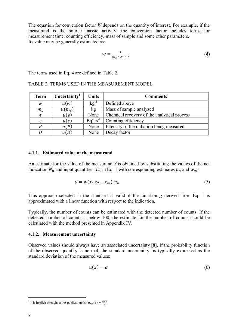
The equation for conversion factor W depends on the quantity of interest. For example, if the measurand is the source massic activity, the conversion factor includes terms for measurement time, counting efficiency, mass of sample and some other parameters. Its value may be generally estimated as: � = �AD.E.F.G.H (4)

The terms used in Eq. 4 are defined in Table 2. TABLE 2. TERMS USED IN THE MEASUREMENT MODEL

Term Uncertainty1 Units Comments � �� kg-1 Defined above I ��I� kg Mass of sample analyzed J ��J� None Chemical recovery of the analytical process K ��K� Bq-1.s-1 Counting efficiency L ��L� None Intensity of the radiation being measured M ��M� None Decay factor

4.1.1. Estimated value of the measurand

An estimate for the value of the measurand Y is obtained by substituting the values of the net indication @$ and input quantities �A in Eq. 1 with corresponding estimates '$ and �A: � = ��,�5 … �A�. '$ (5)

This approach selected in the standard is valid if the function g derived from Eq. 1 is approximated with a linear function with respect to the indication. Typically, the number of counts can be estimated with the detected number of counts. If the detected number of counts is below 100, the estimate for the number of counts should be calculated with the method presented in Appendix IV. 4.1.2. Measurement uncertainty

Observed values should always have an associated uncertainty [8]. If the probability function of the observed quantity is normal, the standard uncertainty1 is typically expressed as the standard deviation of the measured values: �� = N (6)

1 It is implicit throughout the publication that �� = O�P�P .

9

In this case, 68% of the measurements of � will fall within the limits bounded by Q� − ��R and Q� + ��R. Expanded uncertainty limits are obtained by multiplying the standard uncertainty by the coverage factor 0. The probabilities related to different coverage factors are presented in Table 3. The probabilities corresponding to the one-sided intervals may be obtained by dividing the probability values in Table 3 by 2. For example, 34% of the measured values will fall within the limitQ� − ��R to Q�R. The uncertainty estimation in radiation measurements is discussed in detail in Appendix I.

TABLE 3. PROBABILITIES CORRESPONDING TO CERTAIN COVERAGE FACTORS WHEN TWO-SIDED CONFIDENCE INTERVALS ARE USED

Value Probability Comments

1.00 0.683 Approximately 1 in 3 measurements will fall outside these limits.


1.96 0.950 Approximately 1 in 20 measurements will fall outside these limits; commonly called the ‘95% confidence limit’ or the ‘1.96 sigma confidence interval’.

2.00 0.954

Approximately 1 in 22 measurements will fall outside these limits; violation of this limit in quality control measurements warns that the process may be out of control and should be investigated. The use of this coverage factor is recommended by many national measurement institutes. Commonly called the ‘2 sigma confidence interval’.


3.00 0.997

Approximately 1 in 370 measurements will fall outside these limits; violation of this limit in quality control measurements warns that the process is out of control and must be investigated without delay. Commonly called the ‘3 sigma confidence interval’.



The standard uncertainty of the estimated value of the measurand is calculated from the following equation:

�� = T�5. �5�'$� + '$5 . �5�� (7)

The equation assumes that all input quantities are uncorrelated and the function for y is linear. The uncertainty of w corresponding to Eq. 4 is:

�� = �. T��5 �(I� + ��5 �I� + ��5 �J� + ��5 �K� + ��5 �L� + ��5 �M� (8)

10

and thus:

�� = �. T��5 �'$� + ��5 �(I� + ��5 �I� + ��5 �J� + ��5 �K� + ��5 �L� + ��5 �M�

(9)

The foregoing general approach will be used (with modification) throughout the publication.

4.1.3. Net number of counts

In counting and region-of-interest (ROI) analysis, the net number of counts (@$) is calculated from the gross number of counts (@%) and the number of background counts (@&):

@$ = @% − @& (10)

Therefore, an estimate for the net number of counts and its uncertainty are obtained as:

'$ = '% − '& (11)

��'$� = U�5:'%; + �5�'&� = T'% + �5�'&� (12)

The measurand is solved by applying these formulas to Eqs 5 and 7:

� = �. �'% − '&� (13)

�� = U�5. V'% + �5�'&�W + �'% − '&�5. �5 �� (14)

In counting experiments, the number of background counts ('&) is estimated from a separate blank measurement. Let 'X be the number of counts detected in a blank measurement within measurement time (X. If the duration of the source measurement is (I, then:

'& = YDYZ . 'X (15)

Spectrum deconvolution software typically directly reports the net number of counts and its uncertainty. 4.1.4. Well-known background

In certain cases, the background in a radiation measurement can be considered to be well known. Then the uncertainty of the estimated value of the background does not need to be taken into account (��'&� ≈ 0). In counting experiments, this simplification is often made if the blank measurement used to determine the number of background counts is considerably longer than the source measurement. An estimate for the measurand is obtained by applying ��'&� = 0to Eqs 13 and 14:

� = �. �'% − '&� (16) �� = T�5. '% + �'% − '&�5. �5�� (17)

11

4.1.5. Paired measurement

Paired measurement refers to a counting experiment where the measurement time in source and the background measurement are equal ((I = (X�, which directly yields to:

'& = 'X (18)

An estimate for the measurand is obtained by applying this to Eqs 13 and 14:

� = �. �'% − 'X� (19)

�� = T�5. '% + �5. 'X + �'% − 'X�5. �5�� (20)

4.2. STANDARD UNCERTAINTY AS A FUNCTION OF THE MEASURAND (��) To calculate the decision threshold and detection limit, the standard uncertainty of the measurand is needed as a function �� of the true value of the measurand.

In counting and ROI analysis where:

� = ��@% − @&� (21)

The function for �� is obtained by substituting '% with \�] + '& in Section 4.1, Eq. 14:

�� = U�. �� + �5. '& + �5. �5�'&� + V\]W5 . �5�� (22)

If �� = 0, then: �� = 0� = T�5. '& + �5. �5�'&� (23)

The equation for �� cannot always be explicitly specified. This is especially true if the value of @$ is obtained from a spectrum deconvolution software. The topic is discussed in Section 5.4.

4.3. DECISION THRESHOLD (^∗) Decision threshold: The physical effect quantified by the measurand is decided to be

present if the value of the measurand exceeds the decision threshold. In ISO 11929:2010, this is derived as:

�∗ = 0�_` . ��0� (24)

where ��0�is the uncertainty estimate for the background.

12

In counting and ROI analysis, ��0� is obtained from Eq. 23 in Section 4.2:

�∗ = 0�_` . T�5. '& + �5. �5�'&� (25)

Note that the function depends on the uncertainty of the background ��'&� but not on the uncertainty of the other input quantities ��. Since the test is performed for whether or not �∗is exceeded, the value of 0�_` corresponds to one-sided confidence intervals. Therefore, the false detection probability of 5% is obtained by using 0 = 1.645.

4.3.1. Well-known background

If the background is well known, then: �∗ = 0�_` . �. T'& (26) 4.3.2. Paired measurement

If a particular measurement is paired with a particular background, then a factor √2 is introduced: �∗ = 0�_` . �. T2. 'X (27)

4.4. DETECTION LIMIT (^#)

Detection limit: Smallest true value of the measurand which can still be detected with the applied measurement procedure; this determines whether or not the measurement procedure satisfies the requirements and is therefore suitable for the intended measurement purpose. In ISO 11929:2010, this is derived as:

�# = �∗ + 0�_e . ��#� (28)

In counting and ROI analysis, ��#� is obtained from Eq. 22 in Section 4.2:

�# = �∗ + 0�_e . T�. �# + �5. '& + �5. �5�'&� + ��# �⁄ �5. �5�� (29)

0�_e corresponds to one-sided confidence intervals. The term �# appears on both sides of the equation and can either be solved iteratively or explicitly. 4.4.1. Well-known background

With well-known background, Eq. 29 simplifies to:

�# = 0��_`� . �. T2. '& + 0��_e�. U�. �# + �2. '0 + V�#� W2 . �2�� (30)

13

If 0��_`� = 0��_e�, the explicit solution is:

�# = �.]Yg . :�h5.T$g;3�_:�.Oijk�]�;l6 (31)

Note that this solution will converge towards the well-known Currie analysis [9] if 0. ��m� ≪ 1.

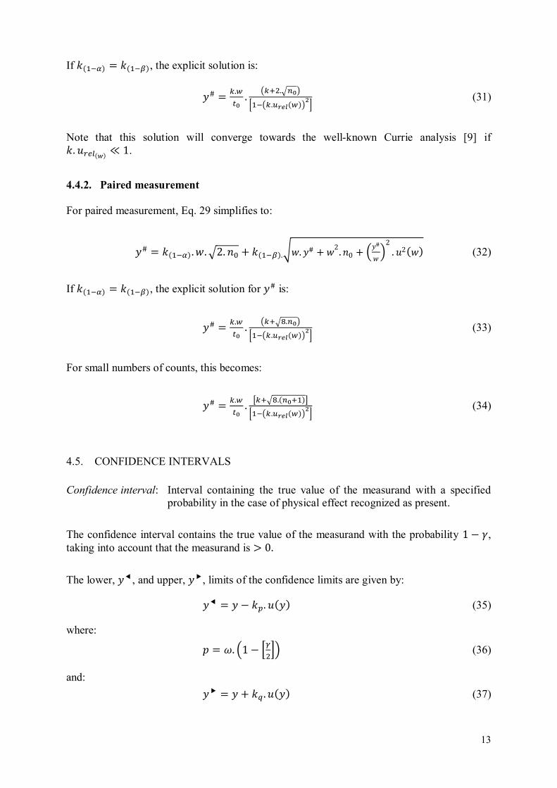
4.4.2. Paired measurement

For paired measurement, Eq. 29 simplifies to:

�# = 0��_`� . �. T2. '& + 0��_e�.U�. �# + �2. '0 + V�#� W2 . �2�� (32)

If 0��_`� = 0��_e�, the explicit solution for �# is:

�# = �.]Yg . :�hTo.$g;3�_:�.Oijk�]�;l6 (33)

For small numbers of counts, this becomes:

�# = �.]Yg . p�hTo.�$gh��q3�_:�.Oijk�]�;l6 (34)

4.5. CONFIDENCE INTERVALS

Confidence interval: Interval containing the true value of the measurand with a specified probability in the case of physical effect recognized as present.

The confidence interval contains the true value of the measurand with the probability 1 − /, taking into account that the measurand is > 0.

The lower, ��, and upper, ��, limits of the confidence limits are given by:

�� = � − 01. �� (35)

where: 2 = r. V1 − 3456W (36)

and: �� = � + 07. �� (37)

14

where: 8 = 1 − 3s.45 6 (38)

Formally, it can be stated:

r = t �√5.u . v wx_yll z.V {|�{�W_} ~�� = 9 3 \O�\�6 (39)

This can be simply calculated in Excel (above 2010) as:

r = 9 3 \O�\�6 = '�). �. ~ �( 3V \

O�\�W , ()�w6 (40)

The values of 01 and 07 are similarly calculated in Excel (above 2010) as:

0$ = '�). �. '��'� (41)

As before, '�). �. ~ �( may be replaced by '�)�~ �( and '�). �. '� may be replaced by '�)� '� in Excel below 2010. The variation of these parameters with

\O�\� is shown

graphically in Figs 1 and 2 (the region where \

O�\� < 1 can be ignored).

FIG. 1. Variation of ω, kp and kq where γ = 4.55% for y/u(y) between 1.0 and 4.0.

0.8

1.0

1.2

1.4

1.6

1.8

2.0

2.2

1.0 1.5 2.0 2.5 3.0 3.5 4.0

Pa

ram

ete

r v

alu

e

y/u(y)

Variation of ω, kp and kq where γ = 4.55%

ω kp kq

15

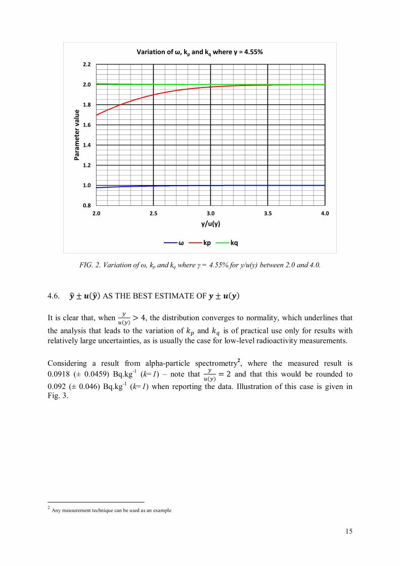
FIG. 2. Variation of ω, kp and kq where γ = 4.55% for y/u(y) between 2.0 and 4.0.

4.6. � ± �� AS THE BEST ESTIMATE OF ^ ± ��^�

It is clear that, when \O�\� > 4, the distribution converges to normality, which underlines that

the analysis that leads to the variation of 01 and 07 is of practical use only for results with relatively large uncertainties, as is usually the case for low-level radioactivity measurements.

Considering a result from alpha-particle spectrometry2, where the measured result is 0.0918 (± 0.0459) Bq.kg-1 (k=1) – note that

\O�\� = 2 and that this would be rounded to

0.092 (± 0.046) Bq.kg-1 (k=1) when reporting the data. Illustration of this case is given in Fig. 3.

2 Any measurement technique can be used as an example

0.8

1.0

1.2

1.4

1.6

1.8

2.0

2.2

2.0 2.5 3.0 3.5 4.0

Pa

ram

ete

r v

alu

e

y/u(y)

Variation of ω, kp and kq where γ = 4.55%

ω kp kq

16

FIG. 3. Distribution and mean for a given massic activity.

From the plot of the data distribution, it is immediately clear that there is a significant portion of the distribution that lies below zero, as is indicated by the ratio

\O�\�. In this case, the

calculation of 01 and 07 is necessary, leading to a modified data plot, which has a discontinuity, due to the differences between 01 and 07.

The modified plot is shown in Fig. 4.

0.000

0.001

0.002

0.003

0.004

0.005

-0.0918 -0.0459 0.0000 0.0459 0.0918 0.1378 0.1837 0.2296 0.2755

Bq kg-1

Distribution of 0.0918 (± 0.0459) Bq.kg-1

Data Mean

17

FIG. 4. Distribution and mean for a given massic activity, modified with kp and kq.

This discontinuity is modified by making a best estimate, ��, of the result. This is calculated as:

�� = � + O�\�.�� {l3l.:|�{�;l6�

s.√5.u (42)

In this case, the uncertainty of ��, ��, is smaller than the measurand uncertainty, ��, and may be calculated as:

�� = T�5�� − �� − ��. �� (43)

As shown from the distribution plot for �� ± ��, it is clear that the data distribution is continuous, with an increase to the value of mean, and a reduction in the uncertainty3.

3 It may be noted that repeated iterations increase �� and decrease �� with constant values being reached after a number of iterations, dependent on the magnitude of � and ��.

0.000

0.001

0.002

0.003

0.004

0.005

-0.0918 -0.0459 0.0000 0.0459 0.0918 0.1378 0.1837 0.2296 0.2755

Bq kg-1

Distribution of 0.0918 (± 0.0459) Bq.kg-1, modified with kp and kq

Data (kp) Mean Data (kq)

18

The modified plot for continuity is given in Fig. 5.

FIG. 5. Distribution and mean for a given massic activity, modified for continuity.

This does change the output data, but only when \O�\� < 4. If the ratios

\�\ and O�\��O�\� are plotted

against \O�\�, then it is clear that �� and �� deviate increasingly from � and �� as the

relative uncertainty of � increases, although the region \O�\� < 1 can be ignored. This is

important for reporting results in the region �# < \O�\� < 4.

These results are illustrated in Figs 6 and 7.

0.000

0.001

0.002

0.003

0.004

0.005

-0.0918 -0.0459 0.0000 0.0459 0.0918 0.1378 0.1837 0.2296 0.2755

Bq kg-1

Distribution of 0.0918 (± 0.0459) Bq.kg-1, modified to 0.0944 (± 0.0432)

Data for y Original Mean Series5

19

FIG. 6. Comparison between y and ŷ for y/u(y) between 1.0 and 4.0.

FIG. 7. Comparison between y and ŷ for y/u(y) between 2.0 and 4.0.

0.90

0.95

1.00

1.05

1.10

1.0 1.5 2.0 2.5 3.0 3.5 4.0

Ra

tio

or

�: �

�/�(�)

Comparison between � and �

Activity ratio Uncertainty ratio

0.93

0.94

0.95

0.96

0.97

0.98

0.99

1.00

1.01

1.02

1.03

2.0 2.5 3.0 3.5 4.0

Ra

tio

or

�: �

�/�(�)

Comparison between � and �

Activity ratio Uncertainty ratio

20

4.7. TOOLKIT

The toolkit given in Table 4 assists with the calculations carried out in this section. Where a spreadsheet function facilitates calculation, it is stated. Reporting results is discussed fully in Section 6.

21

TABLE 4. TOOLKIT FOR RELEVANT CALCULATIONS Quantity Source Equation Comments � Result Varies From measurement calculations �� Uncertainty of � Varies From measurement calculations '*

Number of background counts

'X. (I(X From measurements

0 Coverage factor None Set by user. Assumed double sided – must use equivalent

single sided value for �∗ and �#

'∗ Decision threshold

in counts

0. T'& Well-known background 0. T2. 'X Paired measurement 0. T2. �'X + 1� Small numbers of counts

�# Detection limit

0. �p0 + 2. T'&q31 − :0. ��;56 Well-known background

0� p0 + T8. 'Xq31 − :0. ��;56 Paired measurement

0� p0 + T8. �'X + 1�q31 − :0. ��;56 Small numbers of counts

/ Risk of exceeding quoted confidence

limits None Set by user

r Required to

calculate 2 and 8 9 � �� Use '�). �. ~ �( V3 \O�\�6 , ()�wW

2 Required to calculate 01 r. V1 − 3/26W

8 Required to calculate 07 1 − 3r. /2 6

01 Coverage factor for lower confidence

limit Complex Use '�). �. '��2�

07 Coverage factor for

another lower confidence limit

Complex Use '�). �. '��8�

�� Lower confidence

limit 01. ��

�� Upper confidence

limit 07. ��

�� Best estimate of �

when \O�\� < 4 � + ��. w� _\l

35:O�\�;l6�r. √2. �

�� Best estimate of �� when

\O�\� < 4 T�5�� − �� − ��. ��

22

5. TECHNIQUE-SPECIFIC APPROACHES

5.1. GROSS ALPHA/BETA Measurement of gross alpha/beta activity (or total alpha/beta activity) is a widely used method of screening samples for their radioactivity content. However, it is not a metrologically sound technique, as the measurement makes no attempt to determine the individual radionuclides present and to be an effective screening method it requires the radionuclide composition (or fingerprint) to remain relatively constant over time. That said, the advantages of this technique are the rapidity of measurement. With proper trend analysis of time series measurements from a particular source term, gross alpha/beta activity measurements are extremely sensitive to changes in total massic activity or activity concentration and changes in radionuclide composition. It is inadvisable to compare data from different source terms unless it can be shown that the radionuclide composition of both source terms is similar. In this section, gross alpha/beta activity measurements by planchet counting is considered (see ISO 9696:2007, ISO 9697:2008 and ISO 10704:2009 for examples); gross alpha/beta activity measurements by liquid scintillation counting is also possible (see ISO 11704:2010).

5.1.1. Measurement standards

Measurement standards for calibration in gross alpha/beta counting may be prepared from standard solutions, or directly from suitable solid material (such as U3O8).

5.1.1.1. Standards prepared from solutions

The starting point for such preparations is a certified (and thus traceable) standard solution of the radionuclide in question. Additional calculation parameters must be considered and are listed in Table 5.

23

TABLE 5. ADDITIONAL CALCULATION PARAMETERS FOR PREPARATION OF MEASUREMENT CALIBRATION STANDARDS

Symbol Quantity Units Comments

=I Massic activity of standard source

Bq.kg-1 Determined as explained below

��=I� Uncertainty of

massic activity of standard source

Bq.kg-1 Determined as combination of individual uncertainties

=� Massic activity of standard solution

Bq.kg-1 Provided by manufacturer

��=�� Uncertainty of

massic activity of standard solution

Bq.kg-1 Provided by manufacturer

A Mass of matrix

added to solution kg

Direct observation, although may be recorded as grams (g) or milligrams (mg) �

Mass of standard added to solution

kg Direct observation, although may be recorded as grams (g) or milligrams (mg)

��A� Uncertainty of mass of matrix added to

solution kg Taken from certificate

II Mass of standard

source kg

Direct observation, although may be recorded as grams (g) or milligrams (mg) ��II�

Uncertainty of mass of standard source

kg Taken from certificate

Preparation is usually carried out according to the procedures given in ISO 9696:2007 or ISO 9697:2008, i.e. a known amount of standard solution is added to a solution containing a known amount of solid matrix. It is assumed that upon evaporation the added radioactive standard is homogeneously distributed throughout the solid matrix. Thus:

=I = �i.AiA� (44)

and:

��=I� = =I. UVO��i��i W5 + VO�Ai�Ai W5 + VO�A��A� W5 (45)

5.1.1.2. Standards prepared from solids

This is simpler than the production of standards from solutions, but more reference data are required. The massic activity of a radioactive solid is given as:

=I = V�j.��A� W . VA�.BjA� W . V�� 5� W (46)

24

The additional terms encountered in this equation are listed in Table 6.

TABLE 6. ADDITIONAL CALCULATION PARAMETERS


=� Isotopic abundance

of nuclide

Available from data tables

��=�� Uncertainty of

isotopic abundance of nuclide

� Atomic mass of

nuclide kg.mol-1

�� Uncertainty of atomic mass of

nuclide kg.mol-1

�� Avogadro constant4 mol-1 �� Uncertainty of

Avogadro constant mol-1

� Molecular mass of nuclide compound

kg.mol-1

�� Uncertainty of

molecular mass of nuclide compound

kg.mol-1

�X Decay branching

ratio

��X� Uncertainty of

decay branching ratio

�� Moles of nuclide

element per mole of compound

Available from data tables or knowledge of chemical composition

��

Uncertainty of moles of nuclide

element per mole of compound

Usually nil, unless the compound is known to be non-stoichiometric (this may be the case for uranium oxide)

T1/2 Half-life of nuclide s Available from nuclear data tables �:��/5; Uncertainty of

half-life s Available from nuclear data tables

The expression simplifies to: =I = �j.Bj.�� .�� 5A�.�¡/l (47)

In the case of a pure element, this simplifies to: =I = �j.�� .�� 5Aj.�¡/l (48)

4 The number of atoms is dimensionless and not given units.

25

The uncertainty on ��=I� is:

��=I� = =I. ¢VO��j��j W5 + xO:�¡/l;�¡/l z5 + VO�Aj�Aj W5 + VO�� W5 (49)

In practice, the terms O�Aj�Aj and

O�� are much smaller than O:�¡/l;�¡/l and

O��j��j and can be

ignored, thus:

��=I� ≈ =I. ¢VO��j��j W5 + xO:�¡/l;�¡/l z5 (50)

In the case of beta emission observed in 40K decay, a branching ratio must be applied, so that:

=IV £¤¥g W = �j .Bj .¦Z.�� .�� 5A�.�¡/l (51)

and:

� §=IV £¤¥g W¨ ≈ =IV £¤¥g W . ¢VO��j��j W5 + xO:�¡/l;�¡/l z5 + VO�¦Z�¦Z W5 (52)

5.1.1.3. Use of standards prepared from solutions or solids

Standards are used to prepare calibration sources for the detector system in use. It is advisable to prepare a number of sources (>10), since most gross alpha/beta counters have several channels; a few ‘spare’ sources may be useful for replacing sources rendered unusable during use. Each source ( ) may be measured in each detector channel (©), and a mean of the data taken. For the Yª source in the ©Yª channel:

K�,« = t¬D�,®�¯D�,®� _¬g�®�¯g�®� ��D.ADD (53)

is derived.

A mean value for the efficiency in the ©Yª channel, K�,« , may be calculated using either an unweighted mean, in which case the standard deviation of the mean gives the uncertainty on the efficiency, ��K�. If desired, a weighted mean may be calculated, using the square of the uncertainty on counting as the weighting factor, in which case the uncertainty from weighing, ��I�, and the massic activity, ��=I�, must be combined with the uncertainty from the weighted mean to give ��K�.

26

5.1.2. Gross alpha/beta in solids

This is the simplest measurement, and it requires very little sample preparation and data analysis. The calculation of the massic activity is straightforward, and is expressed by:

=� = �¬AD.F (54)

There are no additional parameters to be considered, although the derivation of the measurement efficiency, K, requires further analysis.

Now the formula used in ISO 9696:2007 yields to:

=� = :�°_�g;�AD.F� (55)

There are four main contributors to the calculation of =�, and these are: )%, )&, I and K. Using the format derived in Appendix I:

��=�� = U�5. 3V�°YD W + V�gYgW6 + =�5 . ��5 �� (56)

is obtained.

Substituting terms, this becomes:

��=�� = UV �AD.FW5 . 3V�°YD W + V�gYgW6 + =�5 . �VO�F�F W5 + VO�AD�AD W5� (57)

When (& = (I, the expression simplifies to:

��=�� = U3 �YD.�AD.F�l6 . :)% + )&; + =�5 . �VO�F�F W5 + VO�AD�AD W5� (58)

If expressed in terms of counts, the expression reads:

��=�� = UV �AD.FW5 . 3V$DYDlW + V$gYgl W6 + =�5 . �VO�F�F W5 + VO�AD�AD W5� (59)

and for (& = (I:

��=�� = UV �YD.AD.FW5 . �'I + '&� + =�5 . �VO�F�F W5 + VO�AD�AD W5� (60)

is obtained.

27

5.1.3. Gross alpha/beta in liquids

This is more complicated, since a liquid sample is used to prepare a solid source. This may be done in two ways — direct evaporation onto the counting substrate (for small volumes of liquid, typically <10 mL), or by the evaporation of a large volume of liquid (>10 mL) to produce a solid for counting. The calculation of the activity concentration is straightforward, and is expressed by:

>� = �¬.A± .Ai.F (61)

The terms encountered in this equation are listed in Table 7. TABLE 7. ADDITIONAL CALCULATION PARAMETERS


²Y Volume of liquid sample

dm3 Volume of sample used to produce ignited solid. Other units can be used – dm3 and L are interchangeable. ��²Y� Uncertainty of ²Y dm3 Derived from tolerances on glassware supplied by the manufacturer.

� Mass of ignited residue from volume ²Y

g Direct observation. It is possible to use milligrams as unit of measure. �� Uncertainty of � g Taken from calibration certificate

� Mass of ignited residue used for counting

g Direct observation. It is possible to use milligrams as unit of measure.

�� Uncertainty of � g Taken from calibration certificate

Preparation is usually carried out according to the procedures given in ISO 9696:2007 [6].

There are six main contributors to the calculation of >�, and these are: )%, )&, �, �, ²Y and K.

Using the format derived in Appendix I, the uncertainty is:

��>�� = U�5. 3V�°YD W + V�gYgW6 + >�5. ��5 �� (62)

Substituting terms, this becomes:

��>�� = UV �AD.FW5 . 3V�°YD W + V�gYgW6 + >�5. �VO�F�F W5 + VO�A�A W5 + VO�Ai�Ai W5 + VO�± �± W5� (63)

When (& = (I, the expression reduces to:

��>�� = U� �YD . V A± .Ai.FW5� . :)% + )&; + >�5. �VO�F�F W5 + VO�A�A W5 + VO�Ai�Ai W5 + VO�± �± W5� (64)

28

If expressed in terms of counts, the uncertainty reads:

��>�� = UV A± .Ai.FW5 . 3V$DYDlW + V$gYgl W6 + >�5. �VO�F�F W5 + VO�A�A W5 + VO�Ai�Ai W5 + VO�± �± W5� (65)

In case (& = (I , the uncertainty simplifies to:

��>�� = UV AYD.± .Ai.FW5 . �>I + >&� + >�5. �VO�F�F W5 + VO�A�A W5 + VO�Ai�Ai W5 + VO�± �± W5� (66)

5.2. ALPHA-PARTICLE SPECTROMETRY

5.2.1. Alpha-particle spectrometry with region-of-interest (ROI) method

Determination of alpha-emitting radionuclides is usually achieved by alpha-particle spectrometry. The technique is metrologically sound as it is used to determine individual isotopes of particular elements by a combination of radiochemical separations to isolate the element of interest, followed by purification, concentration and source preparation before measurement. In this section, alpha-particle spectrometry without spectrum deconvolution is considered as, in many cases, poorly resolved spectra may be rejected by the laboratory’s quality system. An example of an alpha spectrum that can be analyzed with simple region-of-interest (ROI) method without a need for spectrum deconvolution is presented in Fig. 8. In any case, the measurement of very low activities leads to spectra with very few events and in this case spectrum deconvolution is not possible. There are some cases, notably the measurement of complex mixtures of uranium or the measurement of solids, where poor resolution is tolerated, and therefore a different approach is required; this is detailed in Section 5.2.2.

FIG. 8. Example of a simple alpha spectrum that can be analyzed with region-of-interest method.

29

The massic activity calculation is: =� = �¬AD.G.³´,µ.H (67)

and:

��=�� = =� . U��5 �)$� + ��5 �I� + ��5 �L� + ��5 :¶F,E; + ��5 �M� (68)

As before: � = �AD.G.³´,µ.H (69)

and: ��=�� = =� . T��5 �)$� + ��5 �� (70)

In this case, the use of an isotope dilution tracer modifies the calculation of the activity since it is unnecessary to individually determine the chemical yield, J, and the counting efficiency, K, as these can be replaced with the product of the two, ¶F,E, that is determined by the measurement of the tracer. It may, however, be instructive for quality purposes to estimate the values of the chemical yield J and of the counting efficiencyK. These are two additional components to consider.

5.2.1.1. Counting efficiency and chemical recovery

As noted above, isotope dilution techniques can be used to determine chemical yield and counting efficiency. This introduces some additional parameters to the calculations to lead to massic activities. These additional parameters are listed in Table 8.

30

TABLE 8. ADDITIONAL PARAMETERS FOR MASSIC ACTIVITY CALCULATIONS


=Y Massic activity of standard

solution Bq.kg-1 Provided by the manufacturer

��=Y� Uncertainty of massic

activity of standard solution

Bq.kg-1 Provided by the manufacturer

¶F,E Combined chemical yield and counting efficiency

s-1.Bq-1

�:¶F,E; Uncertainty of combined

chemical yield and counting efficiency

s-1.Bq-1

)%,Y Gross tracer count rate s-1 Derived from gross tracer counts and sample count time. ��)%,Y� Uncertainty of gross

sample count rate s-1

)&,Y Tracer background count

rate s-1

Derived from tracer background counts and background count time. ��)&,Y�

Uncertainty of tracer background count rate

s-1 )$,Y Net tracer count rate s-1 Derived from gross and background tracer counts, and sample and background count times. ��)$,Y�

Uncertainty of net sample count rate

s-1 '%,Y Gross tracer count Direct observation �:'%,Y; Uncertainty of gross tracer

count Derived from '%,Y.

'&,Y Tracer background count Direct observation �:'&,Y; Uncertainty of tracer

background count Derived from '&,Y. LY Tracer nuclide intensity

From data tables ��LY�

Uncertainty of tracer nuclide intensity

LI Sample nuclide intensity ��LI� Uncertainty of sample

nuclide intensity MY Tracer decay Derived from tracer half-life and decay

time and sample count time. ��MY� Uncertainty of tracer decay MI Sample decay Derived from sample nuclide half-life and decay time and sample count time. ��MI�

Uncertainty of sample decay

The parameter, ¶F,E, is calculated as follows: ¶F,E = �¯ .A¯��¬,¯ (71)

31

The uncertainty for the tracer activity is derived from the manufacturer’s certificate, and mass uncertainty is detailed in Appendix I, so only the net tracer count rate remains. As before, the gross tracer count rate is: )%,Y = $°,¯YD (72)

with:

�:)%,Y; = U�°,¯YD = T$°,¯YD (73)

Next, the background count rate is: )&,Y = $g,¯Yg (74)

with:

�:)&,Y; = U�g,¯Yg = T$g,¯Yg (75)

It may be useful to calculate the net tracer count rate:

)$,Y = )%,Y − )&,Y = $°,¯YD − $g,¯Yg (76)

with:

�:)$,Y; = U�5:)%,Y; + �5:)&,Y; = U�°,¯YD + �g,¯Yg = U$°,¯YDl + $g,¯Ygl (77)

and:

��5 :)$,Y; = §¬°,¯¯Dl h¬g,¯¯gl ¨V¬°,¯¯D _¬g,¯¯g Wl (78)

In most cases, $°,¯YD ≫ $g,¯Yg , so the expression simplifies to:

��5 :)$,Y; ≈ x¬°,¯¯Dl zV¬°,¯¯D Wl ≈ �$°,¯ (79)

or:

��:)$,Y; ≈ U �$°,¯ (80)

The uncertainty,�:¶F,E;, may be expressed as:

�:¶F,E; = ¶F,E. U��5 �=Y� + ��5 �Y�� + ��5 :)$,Y; (81)

32

5.2.1.2. Calculations of combined uncertainties

This is done as indicated before, such that:

��=�� = >� . U��5 �)$� + ��5 �I� + ��5 :¶F,E; + ��5 �LY� + ��5 �MY� + ��5 �LI� + ��5 �MI� (82)

or

�5�=�� = V �AD.G.¸W5 . 3V$DYDlW + V$gYgl W6 + =�5 . �VO�AD�AD W5 + �$°,¯ + VO��¯��¯ W5 + VO�A¯��A¯� W5 + VO�G �G W5 +VO�GD�GD W5 + VO�HD�HD W5 + VO�H¯�H¯ W5� (83)

In reality, the mass, decay and intensity uncertainties are small as compared to the other sources of uncertainties, so that:

��=�� ≈ ¢V �AD.G.¸W5 . 3V$DYDlW + V$gYgl W6 + =�5 . � �$°,¯ + VO��¯��¯ W5� (84)

and, if (& = (I, the uncertainty reduces to:

��=�� ≈ ¢V �YD.AD.G.¸W5 . �'I + '&� + =�5 . � �$°,¯ + VO��¯��¯ W5� (85)

5.2.2. Alpha-particle spectrometry with spectrum deconvolution software

The simple region-of-interest (ROI) method cannot be applied if the signals from different radionuclides are overlapping in the measured alpha spectrum. Overlapping signals may especially emerge in two situations:

(1) The alpha emission energies of the radionuclides in the sample are close to each other. This can be unavoidable if the sample contains several isotopes of the same element. It can also arise from a failed radiochemical separation of elements.

(2) The self-absorption in the sample matrix leads to the broadening of the alpha peaks. The self-absorption is caused by the thickness of the sample. This may indicate imperfect source preparation.

In these cases, a spectrum deconvolution software code is needed to analyze the activities of individual radionuclides.

33

Figure 9 presents an example of an alpha spectrum with a highly overlapping signal deconvoluted with an alpha spectrum analysis software code. Due to the strong overlap, the spectrum analysis is not possible with a region-of-interest method. To obtain reliable estimates for the nuclide areas and their uncertainties, the analysis process must take the following requirements properly into account:

(1) The areas of the peaks belonging to the same isotope are tied based on the nuclear data.

(2) The correlation between the fitted areas of the overlapping radionuclides increases their uncertainty.

(3) The peak shapes may vary among the samples. Typically, some shape parameters must be individually fitted for each sample.

(4) The α+X, α+e- and α+γ coincidences may influence the peak shape.

5.2.2.1. Calculation of characteristic limits from the area reported by the software

In the best case, the spectrum analysis software can directly calculate the characteristic limits according to ISO 11929:2010 using the methods presented in Annex C of the standard. If the characteristic limits are not given by the software, some estimates must be made. Calculating the characteristic limits from the spectrum analysis results is very similar for both alpha-particle and gamma-ray spectrometry. Therefore, this topic is discussed in detail in the gamma-ray spectrometry section (Section 5.4.3). The only difference is that in alpha-particle spectrometry '$ should be considered to denote the summed area of all alpha transitions of the nuclide of interest.

FIG. 9. Alpha spectrum containing 239

Pu and 240

Pu deconvoluted with Adam software [10].

34

Unlike in gamma-ray spectrometry, utilizing data from a separate blank measurement is typically not feasible in alpha-particle spectrometry (See case 2 in Section 5.4.3). To use this technique, the blank and source samples must be identical, except that the blank sample does not contain the isotope of interest. That means that the activities of all other isotopes in both samples as well as the sample quality must be the same. It should be especially noted that a measurement without a source is not a valid blank measurement in alpha-particle spectrometry, since the main contribution disturbing the analysis comes from the other nuclides in the sample and not from the intrinsic background of the detector. 5.2.2.2. Example

The task is to determine the characteristic limits for the 239Pu activity in a sample. The alpha spectrum of the sample deconvoluted with an analysis software code is presented in Fig. 9. The live time of the measurement (t) was 6.0 hours and the efficiency (ε) was 0.0333 ± 0.0028. The 239Pu area ('$) reported by the software is 23160 ± 2850 counts. In this example, the measurand is the 239Pu activity in the sample. An estimate for the activity is: < = $¬Y.F (86)

and the uncertainty of the estimate is:

��<� = �Y . UV�FW5 . �5�'$� + V$¬Fl W5 . �5�K� (87)

Inserting the given values results in an activity of 32.2 ± 4.8 Bq. Since the activity is over four times larger than its uncertainty, this primary measurement result can also be directly considered as the best estimate. To calculate the decision threshold and detection limit, a function for ��:<¹; is needed. This is obtained from Eq. 143 in Section 5.4.3. The uncertainty of the number of counts (2850) is multiple times larger than the square root of the number of counts (151). Therefore, the criterion set in Eq. 142 is met, and it is justified to estimate that the standard uncertainty as a function of the area is constant: ��'�� ≈ ��'� = 2850.

��:<¹; = �Y . UV�FW5 . ��5�'�$� + <¹5 . �5�K� ≈ �Y . UV�FW5 . �5�'$� + <¹5 . �5�K� (88)

Once the equation for ��:<¹; is known, the decision threshold can be solved with Eq. 24 in Section 4.3:

<∗ = 0�_` . ��:<¹ = 0; = 0�_` . �Y . UV�FW5 . �5�'$� = 8.0Bq (89)

Here, a coverage factor 0�_` = 2.0was selected to obtain a false detection probability of 0.023 (see Table 3 in Section 4.1) Now, it is possible to write an equation for the detection limit based on Eq. 28 in Section 4.4:

<# = <∗ + 0�_e. ��<#� = <∗ + 0�_e . �Y.4 UV�FW5 . �5�'$� + �<#�5. �5�K� (90)

35

A detection limit of 17 Bq is obtained by solving A# from this second-order polynomial

equation. Here, a coverage factor 0�_e = 2.0was selected to obtain a false negative probability of 0.023. 5.3. LIQUID SCINTILLATION COUNTING

The use of liquid scintillation counting has wide application in specific radionuclide determination. The technique is metrologically sound as it is used to determine individual radionuclides that have been isolated from other radionuclides, and then purified and concentrated before measurement.

The massic activity calculation is: =� = �¬AD.F.G.E.H (91)

and: ��=�� = >� . T��5 �)$� + ��5 �I� + ��5 �K� + ��5 �L� + ��5 �J� + ��5 �M� (92)

As before: � = �AD.F.G.E.H (93)

and: ��=�� = =� . T��5 �)$� + ��5 �� (94)

There are two additional components to consider — chemical yield and counting efficiency.

5.3.1. Counting efficiency

This is carried out using standard solutions that are traceable to national or international standards. Usual practice is to prepare a set of standards that exhibit varying amounts of either chemical or color quench as indicated by a suitable indicator, usually called the quench parameter. This enables a plot of counting efficiency against quench parameter to be constructed, such that: K = ¼:½1; (95)

where the form of the function ¼:½1; is not predictable and depends on the spectrum shape, maximum β energy, etc. The additional parameters for the counting efficiency calculations are listed in Table 9. TABLE 9. ADDITIONAL PARAMETERS FOR COUNTING EFFICIENCY CALCULATIONS

Symbol Quantity Comments ¼:½1; Quench parameter curve function Determined empirically � V¼:½1;W Standard uncertainty of the quench parameter

36

In any case, the fit of a suitable function to the observed data will impose an uncertainty on the counting efficiency K in addition to the uncertainty arising from the preparation of the standard sources:

��K� = K. U��5 V¼:½1;W + ��5 �=I� + ��5 �II� (96)

5.3.2. Chemical recovery

Chemical recovery is usually measured by adding a known amount of a suitable tracer at the beginning of the analytical procedure, and then measuring the amount recovered at the end of the analytical procedure, such that: J = A¯iB¯ .A¯� (97)

where: ��J� = J. T��5 �Y�� + ��5 ��Y� + ��5 �Y�� (98)

Additional parameters are listed in Table 10. TABLE 10. ADDITIONAL PARAMETERS FOR RECOVERY CALCULATIONS


�Y Mass concentration

of tracer Provided by the manufacturer

��Y� Uncertainty of mass

concentration of tracer

Provided by the manufacturer

Y� Mass of tracer solution added

kg Direct observation, although may be recorded as grams (g) or milligrams (mg)

��Y�� Uncertainty of mass

of tracer solution added


Y� Mass of tracer

recovered kg

Direct observation, although may be recorded as grams (g) or milligrams (mg) ��Y��

uncertainty of mass of tracer recovered


5.3.3. Calculation of combined uncertainties

This is done as explained before, such that:

��5 �=�� = ��5 �)$� + ��5 �I� + ��5 V¼:½1;W + ��5 �=I� + ��5 �II� + ��5 �L� +��5 �Y�� + ��5 ��Y� + ��5 �Y�� + ��5 �M� (99) In reality, the mass, decay and intensity uncertainties are small in comparison to the other sources of uncertainty, so that:

��5 �=�� ≈ ��5 �)$� + ��5 V¼:½1;W + ��5 �=I� + ��5 ��Y� (100)

37

or:

��=�� ≈ ¢V �AD.F.G.E.HW5 . 3V$DYDlW + V$gYgl W6 + =�5 . ¾§OV¿:ÀÁ;W¿:ÀÁ; ¨5 + VO��D��D W5 + VO�B¯�B¯ W5Â (101)

and, if (& = (I, the uncertainty shortens to:

��=�� = ¢V �YD.AD.F.E.G.HW5 . �'I + '&� + =�5 . ¾§OV¿:ÀÁ;W¿:ÀÁ; ¨5 + VO��D��D W5 + VO�B¯�B¯ W5Â (102)

Examples for the measurement of 90Sr by 90Y ingrowth and for the determination of 241Pu after stripping from an alpha-particle spectrometry source are described below. 5.3.4. Measurement of

90Sr by

90Y ingrowth

This is complicated by the nature of the calculations. Usual practice is to isolate strontium and then to remove yttrium from the isolated strontium recording the time when this is done. Then 90Y is allowed to ingrow for a given time interval, after which it is again separated and then measured; more than one measurement of the 90Y fraction may be made to check radiochemical purity. The activity of 90Y after ingrowth is:

<Ã = �¬�Ä�FÄ.EÄ.HÄ (103)

Then the 90Sr activity in the isolated and purified strontium at the first time of removal of 90Y is given by:

<³� = <Ã . �¡/lÅiV�¡/lÅi_�¡/lÄW . Æw§ÇÈ g.É.¯Ê¡/lÅi ¨ − w§ÇÈ g.É.¯Ê¡/lÄ ¨Ë ≈ <Ã . Æ1 − w§ÇÈ g.É.¯Ê¡/lÄ ¨Ë (104)

and then, the 90Sr activity at the reference time is:

=��³�� = ?ÅiAD.EÅi .HÅi (105)

Overall:

=��³�� = 3 �AD.EÅi .HÅi6 . ¾ �¡/lÅiV�¡/lÅi_�¡/lÄW . Æw§ÇÈ g.É.¯Ê¡/lÅi ¨ − w§ÇÈ g.É.¯Ê¡/lÄ ¨ËÂ . 3 �¬�Ä�FÄ.EÄ.HÄ6 (106)

or

=��³�� = )$�Ã�.ÌÍÍÍÎ �Åi.Ï�§ÇÈ g.É.¯Ê¡/lÅi ¨_�§ÇÈ g.É.¯Ê¡/lÄ ¨Ð

AD.EÅi.HÅi .FÄ.EÄ.HÄ.:�¡/lÅi_�¡/lÄ;ÑÒÒÒÓ (107)

38

and so:

� = �Åi.Ï�§ÇÈ g.É.¯Ê¡/lÅi ¨_�§ÇÈ g.É.¯Ê¡/lÄ ¨ÐAD.EÅi.HÅi.FÄ.EÄ.HÄ .:�¡/lÅi_�¡/lÄ; (108)

approximating:

=��³�� ≈ )$�Ã�. Ô �_�§ÇÈ g.É.¯Ê¡/lÄ ¨AD.EÅi.HÅi.FÄ.EÄ.HÄÕ (109)

and:

� ≈ �_�§ÇÈ g.É.¯Ê¡/lÄ ¨AD.EÅi .HÅi.FÄ.EÄ.HÄ (110)

Additional parameters are listed in Table 11. TABLE 11. ADDITIONAL PARAMETERS FOR THE MEASUREMENT OF 90SR BY 90Y INGROWTH

Symbol Quantity Comments

=��³�� Massic activity of 90Sr in original sample

�:=��³��; Uncertainty of massic activity of 90Sr in original sample

<Ã Activity of 90Y after ingrowth

This is the activity of 90Y at the time of separation of 90Y after ingrowing of the isolated and purified strontium fraction. ��<Ã�

Uncertainty of activity of 90Y after ingrowth

)$�Ã� Net 90Y count rate Determined as in other calculations �:)$�Ã�; Uncertainty of net 90Y count rate Determined as in other calculations KÃ Counting efficiency for 90Y Determined as in other calculations ��KÃ� Uncertainty of counting efficiency for 90Y

Determined as in other calculations JÃ Chemical recovery of yttrium Determined as in other calculations ��JÃ� Uncertainty of chemical recovery of yttrium

Determined as in other calculations

MÃ Decay of 90Y from separation to counting

This is the decay of 90Y between separation and measurement.

��MÃ� Uncertainty of decay of 90Y from separation to counting

Determined as in other calculations, but the uncertainty on the time is:

��(� = ¢(I�1�5�512 + (A��I512

where (I�1�5� is the time taken to separate the 90Y and (A��I is the count time

39

TABLE 11. ADDITIONAL PARAMETERS FOR THE MEASUREMENT OF 90SR BY 90Y INGROWTH (cont.)


<³� Activity of 90Sr before ingrowth

This is the activity of 90Sr at the time of first separation of 90Y before ingrowing. ��<³��

Uncertainty of activity of 90Sr before ingrowth

��/5³� Half-life of 90Sr From data tables ��/5³�� Uncertainty of half-life of 90Sr From data tables ��/5Ã Half-life of 90Y From data tables ��/5Ã� Uncertainty of half-life of 90Y From data tables

(� Ingrowth time Time allowed for 90Y to ingrow into the isolated and purified strontium fraction.

��(�� Uncertainty of ingrowth time

The uncertainty on the time is:

��(�� = ¢(I�1��512 + (I�1�5�5

12

where (I�1�� is the time taken to separate the 90Y from 90Sr before ingrowth J³� Chemical recovery of strontium Determined as in other calculations ��J³��

Uncertainty of chemical recovery of strontium


M³� Decay of 90Sr from sampling to yttrium separation


��M³�� Uncertainty of decay of 90Sr from sampling to yttrium separation


��(� = ¢(I�A512 + (I�1��512

where (I�A is the time taken to obtain the original sample.

5.3.5. Measurement of 241

Pu recovered from plutonium alpha-particle spectrometry

sources This case assumes that the alpha-emitting plutonium isotopes have been determined by alpha-particle spectrometry, using an isotope dilution tracer. For the determination of 241Pu, it is further assumed that the alpha-particle spectrometry source has been dissolved in acid, mixed with liquid scintillation cocktail and measured by liquid scintillation counting, with a low energy region for 241Pu and a higher (and narrow) energy region to determine alpha-emitting plutonium isotopes.

40

The massic activity of 241Pu is given by: =��GO_5Ö�� = �¬�×|�l¥¡�F×|�l¥¡.E×|�l¥¡ .H×|�l¥¡ (111)

Parameters are listed in Table 12. TABLE 12. PARAMETERS FOR CALCULATION OF 241PU RECOVERED FROM PLUTONIUM ALPHA-PARTICLE SPECTROMETRY SOURCES


=��GO_5Ö�� Massic activity of 241Pu in original sample

�:=��GO_5Ö��; Uncertainty of massic activity of 241Pu in original sample

)$�GO_5Ö�� Net 241Pu count rate Determined as in other calculations �:)$�GO_5Ö��; Uncertainty of net 241Pu count rate

Determined as in other calculations )$,` Net alpha channel count rate Determined as in other calculations �:)$,`; Uncertainty of net alpha channel count rate


)$�GO_5ØÙ/5Ö&� Net 239/40Pu count rate from alpha-particle spectrometry


�:)$�GO_5ØÙ/5Ö&�;

Uncertainty of net 239/40Pu count rate from alpha-particle spectrometry


)$,GO_5Øo Net 238Pu count rate from alpha-particle spectrometry


��)$,GO_5Øo�

Uncertainty of net 238Pu count rate from alpha-particle spectrometry


)$,Y Net tracer count rate from alpha-particle spectrometry


��)$,Y�

Uncertainty of net tracer count rate from alpha-particle spectrometry


KGO_5Ö� Counting efficiency for 241Pu Determined as in other calculations ��KGO_5Ö�� Uncertainty of counting efficiency for 241Pu

Determined as in other calculations ��/5GO_5Ö� Half-life of 241Pu From data tables ��/5GO_5Ö�� Uncertainty of half-life of 241Pu From data tables MGO_5Ö� Decay of 241Pu Determined as in other calculations

��MGO_5Ö�� Uncertainty of decay of 241Pu


��(� = ¢��(I�A�512 + ��(A��I�5

12

where (I�A is the time taken to obtain the original sample.

41

As 241Pu is measured by liquid scintillation counting, following measurement of alpha-emitting plutonium isotopes by alpha-particle spectrometry, the following equation applies: =� = �¬AD.F.G.E.H (112)

and:

��=�� = =� . T��5 �)$� + ��5 �I� + ��5 �K� + ��5 �L� + ��5 �J� + ��5 �M� (113) The terms are similar to those before, except that for the recovery, J, which has to be derived from the alpha-particle spectrometry measurements. Now, let the net count rate for alpha-emitting plutonium isotopes (including the tracer, 242Pu) be )$�`�. The value of )$�`� is derived as follows:

)$�`� = =��GO_5Øo�. I. K` . J + =��GO_5ØÙ/Ö&�. I. K` . J + =Y. Y� . K` . J (114)

or )$�`� = J. K`. :=��GO_5Øo�. I + =��GO_5ØÙ/Ö&�. I + =Y. Y�; (115)

But this is related to the net alpha-particle spectrometry counts, such that:

=��GO_5Øo�. I = �¬�×|�lÚÛ�G.H . �¯.A¯��¬,¯ ≈ �¬�×|�lÚÛ��¬,¯ . =Y. Y� (116)

So:

=��GO_5Ö�� = �¬�×|�l¥¡�AD.F�×|�l¥¡�.G.H . FÜ.�¯ .A¯��¬�Ü� . :�¬�×|�lÚÛ�h�¬�×|�lÚÝ/¥g�h�¬,¯;�¬,¯ (117)

where )$�GO_5Øo�, )$�GO_5ØÙ/Ö&� and )$,Y come from the alpha-particle spectrometry calculations, and so:

��5 :=��GO_5Ö��; = ��5 :)$�GO_5Ö��; + ��5 �I� + ��5 :K�GO_5Ö��; + ��5 :L�GO_5Ö��; +��5 :M�GO_5Ö��; + ��5 �K`� + ��5 �=Y� + ��5 �Y�� + ��5 :)$�`�; + ��5 �J� (118)

But the mass, decay and intensity uncertainties are small in comparison to the other sources of uncertainty, so that:

��5 :=��GO_5Ö��; ≈ ��5 :)$�GO_5Ö��; + ��5 :K�GO_5Ö��; + ��5 �K`� + ��5 �=Y� +��5 �Y�� + ��5 :)$�`�; + ��5 �J� (119)

and:

��5 �J� ≈ �:$�×|�lÚÛ�h$�×|�lÚÝ/¥g�h$¯; + �$¯ (120)

Again the terms '�L�−238�, '�L�−239/40� and '( come from the alpha-particle spectrometry calculations and the other terms are calculated as explained before.

42

5.4. GAMMA-RAY SPECTROMETRY Gamma-ray spectrometry is a powerful technique with a high selectivity to quantify gamma-emitting radionuclides. The selectivity of the method depends on the detector. For laboratory analysis high-purity Germanium detectors (HPGe) are usually used. For screening purpose or analysis of simple spectra, other detectors like sodium iodide NaI(Tl) can be used. For analysis of gamma-ray spectra, a dedicated software is generally operated. This software also has the options to set up the different calibrations (e.g. energy, peak shape, counting efficiency, peak-to-total efficiency, etc.). Once the calibration parameters have been set, radionuclides can be identified in the spectrum and their activity can be determined. The information obtained from a basic spectrum analysis is represented by the peak position (expressed in terms of gamma-ray energy), net peak areas and uncertainty of the net peak areas. The number of peaks obtained in a spectrum analysis depends on the peak search algorithms and the parameter settings in these algorithms. Statistical filters evaluating peak data against a decision threshold are used to judge if a peak is to be further used in the analysis or not. The net peak area calculation can also be done in several ways. Two methods can be identified: peak analysis without fitting or peak analysis based on fitting part of the spectrum with a mathematical function. In case of multiplets of overlapping peaks the spectrum deconvolution may be the only option to obtain the peak areas and their uncertainty for individual peaks. The computation of the characteristic limits in gamma-ray spectrometry follows different approaches depending on the specific spectroscopic conditions (e.g. presence of a background peak, presence of interfering peaks). Since the spectrum analysis is done by software there are two options for an ISO 11929:2010 compatible calculation of detection limits: whether the software includes modules to compute these parameters or the software does not. In the latter case this document shows how the characteristic limits can be computed from the basic output of the spectrum analysis, with the condition that the uncertainty has been dealt with in a proper way. 5.4.1. Terminology

Blank indication (for gamma-ray spectrometry)

Indication measured with a blank sample, i.e. in the absence of the sampled material. The counts contributing to the blank indication originate from the background that is intrinsic to the measuring system, from the interference of the net indication with the indications of other analytes being present in the sample and from the response of the measuring system to the analyte, that is present in the blank sample. The analyte may be present in the auxiliary materials in the sample, i.e. the materials that were not sampled but are used to preserve the integrity of the sample. Continuous background

Background in the spectrum, on which the peaks reside. The change of the height of the continuous background in an energy interval having the width of a spectral peak is small as compared with the uncertainty of the number of counts in one channel.

43

Decay factor

The correction factor that transforms the activity corresponding to the indication to a reference time, this is usually the sampling time. This factor may comprise three contributions: the decay during the sample collection period, the decay between the end of sampling and start of spectrum acquisition and the decay during the spectrum acquisition. The correction factor depends on the half-life of the analyte but may comprise also half-lives of other radionuclides if the analyte belongs to a decay chain. Full-energy peak efficiency

The counting efficiency describing the probability that the gamma- or X-ray interacts within the sensitive volume of the detector in such a way that it deposits all its energy there. Interference of indications

Overlapping peaks belonging to different analytes, i.e. peaks occupying overlapping spectral intervals. If the overlap is so tight, that the peak analysing software cannot resolve individual peaks the indications (or the peaks) interfere. Number of counts in a full-energy peak

Registered number of events corresponding to the full absorption of the energy of a gamma-ray in the peak. Synonym: peak area. The unit of this number of counts is unity. Peaked background

Counts in a peak occurring at the same, or very close lying, energy as the peak due to the presence of the analyte in the sampled material. It is due to the influence of the sources of measurement bias. The sources of the peaked background are: the spectrometer, the activity in the blank materials, and spectral interferences. Peak region

Region in the spectrum occupied by a peak. The optimal width of the peak region in region-of-interest analysis depends on the measured spectrum. The standard ISO 11929:2010 recommends to use a region 2.5 times the full width at half maximum (FWHM) for a pronounced peak and 1.2 times the FWHM in case of dominant background. The background dominates, if the tails of the peak cannot be observed because of the statistical fluctuations of the continuous background. Region-of-interest (ROI)

Spectral region used for calculating the number of counts in a peak in region-of-interest analysis. If the peak is located, it is safe to assume that a region 5 times the FWHM of the peak covers all counts belonging to the peak Self-attenuation factor

The factor expressing the fraction of the gamma-rays emitted by the analyte, which are prevented from registration in the spectrum because of interaction with the sampled material.

44

Sensitivity parameter

Criterion set for differentiating statistical fluctuations of the continuous background from small peaks if the peak analysis is based on a peak locating algorithm. The sensitivity parameter value defines the minimal number of standard deviations of the continuous background from its expected value to recognize a maximum in the continuous background as a peak. Example: The peak analyzing procedure operating with the sensitivity parameter assuming a value of 3 censors peaks with an area less than 3u(ng). Synonym:

significance threshold. Spectral peak

Peak occurring in the spectrum due to the full absorption of the energy of the gamma-ray in the sensitive volume of the detector or an escape peak. Synonym: spectral line.

Interfering peaks

Peaks due to gamma-rays emitted by other gamma-ray emitters in the sample radiating at energies that are too close to the energy of a peak due to the presence of the analyte in the sampled material, to be separated. Spectrometer background

It originates from the presence of gamma-ray emitters in the materials of the spectrometer and from gamma-rays from the environment penetrating the spectrometer shield. Besides to the peaked background it contributes also to the continuous background. This background is also present in the spectrum acquired in the absence of the sample. 5.4.2. Spectrum analysis with region-of-interest method

In some cases it may be interesting to do a quick computation of decision threshold and detection limits based on a simple region-of-interest (ROI) evaluation for a given gamma peak in a spectrum. Parameters are listed in Table 13.

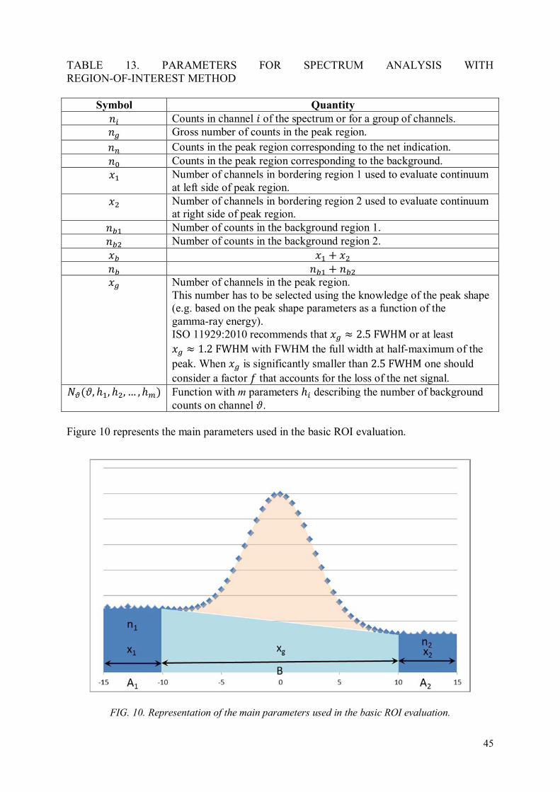
45

TABLE 13. PARAMETERS FOR SPECTRUM ANALYSIS WITH REGION-OF-INTEREST METHOD

Symbol Quantity '� Counts in channel of the spectrum or for a group of channels. '% Gross number of counts in the peak region. '$ Counts in the peak region corresponding to the net indication. '& Counts in the peak region corresponding to the background. �� Number of channels in bordering region 1 used to evaluate continuum at left side of peak region. �5 Number of channels in bordering region 2 used to evaluate continuum at right side of peak region. 'X� Number of counts in the background region 1. 'X5 Number of counts in the background region 2. �X �� + �5 'X 'X� + 'X5 �% Number of channels in the peak region. This number has to be selected using the knowledge of the peak shape (e.g. based on the peak shape parameters as a function of the gamma-ray energy). ISO 11929:2010 recommends that �% ≈ 2.5FWHM or at least �% [ 1.2FWHM with FWHM the full width at half-maximum of the peak. When �% is significantly smaller than 2.5FWHM one should consider a factor ¼ that accounts for the loss of the net signal. @ä�å, ��, �5, … , �A� Function with m parameters �� describing the number of background counts on channel å.

Figure 10 represents the main parameters used in the basic ROI evaluation.

FIG. 10. Representation of the main parameters used in the basic ROI evaluation.

46

The model ��'æ , ��that gives the activity<as a function of the input quantities '$ and � is:

< = ��'$ , �� = '$ . � = :'% − '&;. � (121)

In which: '$ is the net number of counts in the peak ROI; '%is the gross number of counts in the peak ROI; '&is the background number of counts in the peak ROI; � is the value of the conversion function including the measurement time. Compared to the default model suggested in ISO 11929:2010, this is a simplified model that assumes that the gross counts only need correction with one background component. If the estimated values '%,'& and their corresponding uncertainties ��'%�,��'&� are known, the standard uncertainty of the activity is: �5�<� = �5. �5:'%; + �5. �5�'&� + �5��. :'% − '&;5

(122)

The uncertainty of the gross number of counts can be replaced with the square root of the detected number of counts: �5�<� = �5. '% + �5. �5�'&� + �5��. :'% − '&;5

(123)

(a) Estimation of the background in the peak region A value for '& is obtained by integrating the function @ä�å� over the peak region: '& = v @ä�å, ℎ�, ℎ5, … , ℎA�. ~åhP°/5_P°/5 (124)

Assuming a linear background and two bordering regions of equal length (�X� = �X5 = �X), the function for @ä�å� becomes:

ç�å� = $Z¡PZ + x$Zl_$Z¡PZhP° z . Vå − P°5 − PZ5 W (125)

and an estimate of the background contribution to the peak region is then obtained as:

'& = v ç�å�. ~åhP°/5_P°/5 = �'X� + 'X5�. P°5.PZ (126)

Since �% and �X are constants, the uncertainty of '& becomes:

�5�'&� = V P°5.PZW5 . ��5�'X�� + �5�'X5�� = V P°5.PZW5 . �'X� + 'X5� (127)

47

(b) Characteristic limits To calculate decision threshold and detection limit the standard uncertainty of the measurand is needed as a function ��Ẩ�. In ROI analysis, the uncertainty ��'$� is known as a function of '%. Therefore, an explicit equation for ��Ẩ� that does not depend on '% can also be formulated, as explained in Section 4.2. The decision threshold is calculated using Eq. 25 in Section 4.3: <∗ = 0�_` . �. T'& + �5�'&� = 0�_`. �. U�'X� + 'X5�. P°5.PZ . V1 + P°5.PZW (128)

This is the same result as is obtained following the Currie approach [9] based on evaluations of the counts level and multiplied by � to express it in terms of activity.

The detection limit is calculated using Eq. 29 in Section 4.4:

<# = <∗ + 0�_e. U�. <# + �5. '& + �5. �5�'&� + �5��. V?#] W5 (129)

This second-order polynomial equation can be solved in closed form. If 0�_` = 0�_e = 0, the solution has a simple form:

<# = 5.?∗h�l.]�_�l.Oijkl �]� (130)

This solution exists only if 1 − 05. ��5 �� > 0. It is clear now that <# cannot be obtained directly from the Currie approach [9] based on multiplying the counts with the conversion factor �. However the detection limit in terms of activity (activity concentration or massic activity) is still readily obtained in this case by multiplying the detection limit expressed in counts by the factor

]�_�l.Oijkl �]�. Figure 11 shows 1 − 05 . ��5 �� as a function of �é�� and k = 1.65 or k = 2 respectively.

Figure 12 shows the effect of uncertainty on the weighting function ��_�l.Oijkl �]�.

48

FIG. 11. Variation of the weighting function ê . ëì. �íîïì �ð� as a function of �íîï�ð� for k=1.645

and k=2.0, respectively.

FIG. 12. Effect of �� on the weighting function ��_�l.Oijkl �]� for k=1.645 and k=2, respectively.

The computation of A∗and <#can be done in a similar way for a slightly more complicated situation in which the model is changed to: ò = ��, �5, �Ø, �� = �� . �5 . �Ø�. � (131)

49

In which �Ø now represents an additional background term related to e.g. the correction for a background peak that is observed in a spectrum when measuring a blank sample. It is easily shown that now:

u5�ò� = �5. �'$ + '&+�5�'&� + 'Ø+�5�'Ø�� + ò5. Ol�]�]l (132)

in which �Ø was replaced by counts 'Ø resulting in two additional contributions respectively, 'Ø the counts contributing to the gross signal '% = '$ + '& + 'Ø and �5�'Ø�. The uncertainty ��'Ø� is obtained from the analysis of the peak in the blank spectrum in a similar way as shown above. In cases with clear evidence that results of the blank spectrum vary with time, then it is more appropriate to replace 'Ø with the mean value obtained from a defined number of measurements 'Ø → 'Øõõõ and �5�'Ø� → N5�'Øõõõ�, the standard variation of the mean count. The quantities ò∗and ò# are then obtained, as before, by changing the counts part and accounting for the fact that this background correction may require an additional scaling factor to account for the difference in measurement time between the sample measurement time (I and the background spectrum from which �Ø was obtained with a measurement time (AØ.

�Ø. YDY�Ú + �5�'Ø�. x YDY�Øz5 (133)

When the quantities ò∗and ò# have to be determined in a spectrum where no peak was identified (e.g. the net peak area is below the decision threshold) then there is no need to evaluate the border regions of the ROI of the presumed peak. Then '& is given by: '& = v ç�å�. ~åY°& = ∑ '�A& (134)

Where is the number of channels in the ROI B and: �5�'&� = '& (135)

Then the decision threshold and the detection limit are given by: ò∗ = 0. ��Α = 0� = 0. �. T2. '& (136)

<# = �.].��hTo.$g��_�l.Oijkl �]� (137)

That are the commonly encountered equations for gross counting. The conversion factor � may be typically composed of the following parameters in gamma-ray spectrometry: � = �Y�.E.F.¿ .¿Å.G.H (138)

50

The parameters are listed in Table 14.

TABLE 14. DEFINITION OF PARAMETERS INCLUDED IN THE FUNCTION W

Term Uncertainty Units Comments ò ��Α� Bq Result of the measurement.

� �� s-1 Defined above. Units may vary depending on the measurement quantity considered e.g. activity or activity concentration.

J ��J� None

Sample quantity scaling factor. This factor corrects for the fact that the sample being measured may be the result of a sample treatment that e.g. concentrated or diluted the original sample.

K ��K�

s-1.Bq-1

Reference counting efficiency of the measurement system used corresponding to the counting efficiency of a reference sample that is close to the actual sample counting efficiency. Differences are to be compensated by an efficiency transfer factor.

¼F ��¼F� None

Efficiency transfer factor that corrects for the difference in the counting efficiency of the actual sample and the reference counting efficiency, generally obtained from a basic calibration. The uncertainty of ¼F may depend on many parameters e.g. the uncertainty on the parameters that are responsible for the difference between the sample efficiency and the reference efficiency, but also on the accuracy of the computation of the correction factor e.g. formulae or software used.

¼³ ��¼³� None

True coincidence summing correction factor for the radionuclide considered. This factor and its uncertainty are radionuclide specific and they depend also on sample measurement geometry and density. The uncertainty depends on the procedure used to determine the factor. L ��L� None Intensity of the radiation being measured. M ��M� None Decay factor.

t u(t) s Duration of the acquisition time.

5.4.3. Calculation of decision thresholds and detection limits according to

ISO 11929:2010 using peak analysis results

In the best case, the spectrum analysis software can directly calculate the characteristic limits according to ISO 11929:2010 using the methods presented in Annex C of the standard. If the characteristic limits are not given by the software, some estimates are needed to calculate these values starting from the other parameters. In principle, the decision threshold and detection limit are calculated using Eq. 24 in Section 4.3 and Eq. 28 in Section 4.4 respectively. However, to use these equations, the standard uncertainty of the measurand is needed as a function ��. Unfortunately, if the spectrum is analyzed with a deconvolution software, this function is typically not directly available, but needs to be estimated from the measurement results.

51

This section presents how the function �� can be estimated from the peak areas reported by the software. To use the presented technique, the software needs to calculate correctly uncertainty estimates for these parameters. It is especially important that the analysis software can properly take into account the correlations between the fitted parameters. Reliable uncertainty estimates can be obtained by performing spectrum deconvolution with a method similar to the one presented in Section C.5.4 (Annex C) of the ISO 11929:2010 standard. The measurement model used in this subsection is of the simplified form presented in Eq. 2 in Section 4.1. However, the results can also be generalized for the generic measurement model given in Eq. 1. In gamma-ray spectrometry, @$ denotes the area of the peak of interest and '$ ± ��'$� the corresponding value given by the analysis software. The estimated value of the measurand is calculated using Eq. 5 and its uncertainty using Eq. 7: � = �:��,�5 … �B;. '$ (139)

�� = T�5. �5�'$� + '$5 . �5�� (140)

(a) Single measurement If only a single measurement has been performed, the function �� is estimated from the peak area '$ and its uncertainty ��'$� reported by the software for this measurement. The ISO 11929:2010 standard suggests to approximate the uncertainty function ��'�$� with a

constant independent of n~: ��'�$� = ��'$� (141)

The constant approximation is valid if ��'$� is dominated by the background counts and not by the area of the peak itself:

��'$� ≫ T'$ (142)

An estimate for �� is obtained from Eq. 139 using the constant approximation and the substitution '�$ = ��/�:

�� = U�5. �5�'$� + V\�]W5 . �5��A� (143)

If �� = 0, the equation simplifies to the form:

�� = �. ��'$� (144)

If the area '�$ contributes significantly to the uncertainty ��'�$�, the constant approximation is incorrect. By taking into account the contribution of the peak area, we obtain:

��'�$� = T�5�'$� − '$ + '�$ (145) and:

�� = U�5. ø�5�'$� − '$ + \�]ù + V\�]W5 . �5��A� (146)

52

(b) Separate source and blank measurement The decision threshold and detection limit can be determined more precisely if also a blank measurement without the isotope of interest is available. The samples used in the source and the blank measurement must be identical, except that the blank sample does not contain the radioisotope of interest. If the peak areas and their uncertainties from a blank measurement and source measurement equal in time are available, the ISO 11929:2010 standard suggests a linear interpolation of the quadratic uncertainty as follow:

�!2�'!� = �2�0� + �2�''�−�2�0�'' . '!' (147)

and:

�� = U�5. ø�5�0� + Ol�$¬�_Ol�&�$¬ . \�]ù + V\�]W5 . �5��A� (148)

5.4.3.1. Example

The task is to determine the characteristic limits for the 241Am activity in a sample. The gamma-ray spectrum of the sample deconvoluted with an analysis software code [10] is presented in Fig. 13. The efficiency (ε) of the detector for the 59.5 keV gamma ray is 0.02 ± 0.001 and the measurement live time (t) 2.0 hours. The intensity (P) of the 59.5 keV gamma ray in 241Am decay is 35.9%. The 241Am peak area reported by the software is 4984 ± 1994 counts.

FIG. 13. Gamma-ray spectrum where the 59.5 keV photopeak of 241

Am has a non-linear baseline.

As can be seen in Fig. 13, the baseline around the 59.5 keV 241Am peak is significantly non-linear. This makes the spectrum analysis challenging and is also the main reason for the high uncertainty of the 241Am peak area.

53

In this example, the measurand is the 241Am activity in the sample. An estimate for the activity can be calculated from the given parameters using the following equation: < = $¬Y.F.G (149)

and the uncertainty of the estimate:

��<� = �Y.G . UV�FW5 . �5�'$� + V$¬Fl W5 . �5�K� (150)

Inserting the given values results in a primary measurement result of 96.4 ± 38.9 Bq. To calculate the decision threshold and detection limit, a function for ��:<¹; is needed. The uncertainty of the number of counts (1994) is multiple times larger than the square root of the number of counts (70.6). Therefore, the criterion in Eq. 142 is met, and the standard uncertainty as a function of the peak area can be approximated to be constant: ( ) 1994~~ ≈nu .

The function for ��:<¹; is obtained from Eq. 142:

��:<¹; = �Y.G . UV�FW5 . ��5�'�$� + <¹5 . �5�K� ≈ �Y.G . UV�FW5 . �5�'$� + <¹5 . �5�K� (151)

The decision threshold is solved by inserting ��:<¹; into Eq. 24 in Section 4.3:

<∗ = 0` . ��:<¹ = 0; = 0` . �Y.G UV�FW5 . �5�'$� = 78Bq (152)

Here, a coverage factor 0�_` = 2.0is selected to obtain a false detection probability of 0.023 (see Table 3 in Section 4.1) Now, an equation for the detection limit based on Eq. 28 in Section 4.4 can be written as follow:

<# = <∗ + 0�_e. ��<#� = <∗ + 0�_e . �Y.G . UV�FW5 . �5�'$� + �<#�5. �5�K� (153)

A detection limit of 160 Bq is obtained by solving A# iteratively from this equation.

The best estimate of the activity is calculated from the primary measurement result using Eq. 42 in Section 4.6:

Aû = A + ü�ý�∙�� ll.�l��.�.�.√5.� (154)

And its uncertainty using Eq. 43 in Section 4.6:

�:<; = U�5�<� − :< − <;. < (155)

These equations result in the best estimate of the activity of 97 ± 39 Bq, which is the same as the primary measurement result used in the calculations. Thus, the calculation of the best estimate had no practical influence on the outcome and could have been omitted.

54

5.4.4. Correlations for overlapping peaks and uncertainty of the continuous

background

When peaks overlap, their peak areas become correlated. The correlation originates in the requirement, that counts, which contribute to the peak area of one peak, cannot contribute to the peak area of a neighboring peak. Correlations among peak areas become important in calculations of decision thresholds and detection limits when these are calculated by post-processing of peak analysis results, when peaks due to the same measurand overlap. This occurs in calculating decision thresholds and detection limits of X-ray emitters. Here peaks due to Kα and Kβ or Kα1 and Kα2 may overlap. Then, according to the multi-peak approach, the common decision threshold is given as [8]:

222**2121

211

2 *.),(.*.*...2*.*21

ynnryyyy yy νννν ++= (156)

Where ν1 and ν1 denote the weights:

21

22

2

22

21

1

*

*1

1 and

*

*1

1

y

y

y

y+

=+

= νν (157)

However, the peak analyzing software packages, currently available on the market, do not report the covariances among areas of overlapping peaks r(np1,np2). In the absence of the data from the peak analysis on the covariance, the value of the correlation coefficient between areas of peaks located at channels 0201 and ϑϑ may be supposed to be the scalar product

(overlap) of the spectrometer’s response to the gamma rays with energies corresponding to the channels 0201 and ϑϑ :

∑=

−=

m

jjj

AAr1

20201 0201.

..2

1),( ϑϑσπ

ϑϑ (158)

Where j is the channel number of both peak regions. The correlation coefficient is negative, because counts, attributed to one peak, cannot contribute to the neighboring peak, therefore any increase of one peak area automatically decreases the other. It can be observed that the correlation coefficient does not depend on the peak areas, but only on the peak positions and their widths. For closely-spaced peaks the correlation coefficient approaches -1 and for non-overlapping peaks zero. It should be observed that, since the correlation coefficient is negative, it diminishes the common decision threshold. Not only the correlations among quantities appearing in the conversion factor contribute to the common detection limit, but also the correlations among peak areas.

55

5.4.5. Approach based on post-treatment of data obtained from peak analysis software

Table 15 explains the symbols, definitions and corresponding quantities to be used in the post-treatment of gamma-ray peak analysis results. The peak analysis results comprise peak positions, areas and their uncertainties. The uncertainties of the peak areas are commonly used for propagating them into the measurement results. Their use in calculation of the decision thresholds and detection limits presents therefore their use outside their intended purpose. Therefore the gamma-ray peak analysis results should be validated for their suitability for the calculation of decision thresholds and detection limits. The method supposes that the total number of counts corresponds to a peak region with well-defined boundaries. Therefore the software used in the peak analysis must not take into account the uncertainties of the peak start and peak end channels into the uncertainty of the peak area. TABLE 15. SYMBOLS, DEFINITIONS AND QUANTITIES TO BE USED IN THE POST-TREATMENT OF GAMMA-RAY PEAK ANALYSIS

Symbol Definition

(to be used in post-treatment of gamma-ray peak analysis only '1 Indication, number of counts in the peak ��'1� Standard uncertainty of the number of counts in the peak

'& Counts in the peak region, which do not belong to the indication n0 = ng - np, i.e. counts in the continuous background and in the possible tails of the neighboring peaks. ��'&� Standard uncertainty of the number of counts not belonging to the indication ' Counts in the peaked background obtained from a null measurement ��'� Standard uncertainty of counts in the peaked background '$ Counts of the net indication, nn = np - nB ��'$� Standard uncertainty of the net indication

��'$� Standard uncertainty of the null indication taking ��'� into account. Since nB and u(nn) are obtained from separate measurements: �5�'� + �5�'$� = �5 �'$� ' Number of counts '\∗ Number of counts corresponding to the decision threshold ��'\∗� Standard uncertainty of the indication when it equals '\∗ '\# Number of counts corresponding to the detection limit ��'\#� Standard uncertainty of the indication when it equals '\#

��'$ = 0� Standard uncertainty of the net indication if the value of the net indication is zero � Conversion function � Value of the conversion function, conversion factor �� Standard uncertainty of the conversion factor �� Relative uncertainty of the conversion factor �õ Mean value of the measurand ��õ� Standard uncertainty of the mean value of the measurand

r(x1,x2) Coefficient describing the correlation between the quantity values x1 and x2.

56

The information on the activity of a gamma-ray emitter is obtained from the peaks in the spectrum that are associated with the gamma-ray emitter, because the net numbers of counts in the peaks are proportional to the activity in the sample. The measurement model used in gamma-ray spectrometry for calculations of activities is:

WXXXXY ⋅−−= ).( 4321 (159)

where X1 denotes the indication with the value np, X2 the spectrometer background, X3 the shielding factor, X4 the peaked background originating in the sample and W the conversion function. The shielding factor describes the attenuation of the spectrometer background in the material of the sample, therefore its value is less than unity. X4 describes the contributions of the blank sample and of the interfering gamma-ray emitters to the number of counts in the peak. It should be observed that X1-X2.X3 -X4 represents the net indication, which is by the conversion function W converted to the activity or massic activity. The conversion function comprises the intensity, detection probability, duration of the acquisition time, sample quantity, decay correction and the possible correction factors to take into account systematic effects such as coincidence summing effects and factors taking into account departures of the actual counting conditions from the counting conditions in which the efficiency was measured. The values of the input quantities x1, x2, x3 and x4 are associated with uncertainties. The uncertainty of the net indication is the combined uncertainty due to the indication and the sources of peaked background. Since the null measurement uncertainty is given with the uncertainty of the null indication it is important to reduce the uncertainties of the peaked background as much as possible and to assess them realistically. However, any systematic influences appearing because of errors in the peaked background should be taken into account in their uncertainty. In gamma-ray spectra peaks reside on a continuous background. This background must be estimated from spectral regions, where no peak resides. Besides the continuous background also peaked background may be present which is taken into account in the measurement model. In the calculations of the decision threshold and detection limit of a gamma-ray emitter it is assumed that neither the continuous background nor the peaked background depend on the activity of the gamma-ray emitter. The decision threshold is a property of the blank measurement, i.e. it can be directly calculated from the measurement of a blank sample. For a gamma-ray emitter that was not detected in the sample, the measurement of a test sample already presents the measurement of a blank sample. Since no peaks are associated with it, in the calculation of decision threshold the channel contents must be used. If it was detected, the detection limit can still be calculated from channel contents, if the continuous background where the peaks reside can be determined. This can be done in case of isolated peaks, where the continuous background under the peak can be interpolated from the spectral regions below and above the peak that are adjacent to the peak. However, if the peak analysis results associated with the peak are available, the decision threshold can also be calculated from these results.

57

By calculating decision threshold and detection limit, the properties of the null measurement are evaluated. Therefore these calculations present only an assessment, based on the measurement of a test sample. The methods of calculation of the decision threshold represent therefore methods on how to express the uncertainty of the blank indication in terms of quantities calculated from the spectrum of a test sample. 5.4.5.1. Peak analysis

For calculating the decision threshold the function )~(~ yu is needed, but this cannot be obtained directly from the results obtained from the spectrum analysis software. Therefore a method is needed to estimate this function. Since the calculations of decision threshold and detection limit are performed at the end of the spectrum analysis procedure, the results of the peak analysis, the activities of the gamma-ray emitters and the conversion factors are already available. It is better to calculate the decision threshold from the peak analysis results rather than directly from the channel contents, because the peak areas and their uncertainties are calculated also if the peaks overlap. When using data from the peak analysis, the shape of the continuous background is taken into account in the calculation of decision threshold and detection limit, because it was taken into account during the peak analysis. When at an energy E a peak appears, the peak analyzing software reports the number of counts in the peak, np, its uncertainty, u(np), or its relative uncertainty, urel(np). To arrive at the number of counts in the peak region, which do not belong to the peak, n0, the total number of counts in the peak region, ng, must also be known. For isolated peaks, as for the width of the peak region 2.5 FWHM is used and the total number of counts is obtained as the sum of channel contents in the peak region, its uncertainty is u(ng) = ng

1/2. The number of counts, which do not belong to the peak is n0 = ng – np. Since the total number of counts in the peak region in a specific spectrum, i. e. a realization, is fixed, the number of counts in the peak and the number of counts that do not belong to the peak are correlated with the correlation coefficient r(np, n0) having a value of -1, because a number of counts attributed to the continuous background and the tails of the neighboring peaks must not be attributed to the peak. Therefore the uncertainty of the number of counts in the continuous background is given by:

0nnn pg −= (160)

Because np and n0 have a complete negative correlation its uncertainty is:

)()(),(2)()()( 000222 nununnrnununu pppg ⋅⋅⋅−+= (161)

This equation has two solutions:

[ ])()()( 0nununu pg −±= (162)

from where:

)()()( 0 gp nununu ±= (163)

follows.

58

Since ng2 = ng, the uncertainty of the number of counts, which do not belong to the peak is:

gp nnunu ±= )()( 0 (164)

In terms of probability density distributions these equations are illustrated in Fig. 14. The probability density distribution of the number of counts in the peak pp(nnp) is represented by a normal distribution with a mean of np and a standard deviation of u(np). The probability density distribution of the number of counts in the background p0(nn0) is represented by a normal distribution with the mean n0 = ng – np and a standard deviation of u(n0). The probability density distribution of the total number of counts pg(nng) is represented by a normal distribution having a mean of ng and a standard deviation of u(ng) = ng

1/2. Because the number of counts in the background and the number of counts in the peak are correlated with the correlation coefficient -1, a specific value of the number of counts in the peak, i.e. a realization, nnp < np is associated with a specific number of counts in the background nn0 > n0. Because a deviation of the number of counts in the peak from its mean is partially compensated with the deviation of the number of counts in the background in the opposite direction, it is clear, that u(ng) must be smaller than u(np) and u(n0). Therefore two possibilities exist to combine the probability density distributions pp(nnp) and p0(nn0) into pg(nng):

u(n0) < u(np). In this case the influence of p0(nn0) decreases the width of the combined distribution to the value of ng

1/2.

u(n0) > u(np). In this case the influence of pp(nnp) decreases the width of the combined distribution to the value of ng

1/2.

In the specific case illustrated in Fig. 14, it is shown how two distributions for the number of counts in the background p01(nn0) and p02(nn0) are associated with one distribution of the number of counts in the peak pp(np) and one distribution of the total number of counts pg(nng). The total number of counts, the number of counts in the peak and their uncertainties are then ng = 256, u(ng) = ng

1/2 = 16, np = 100, u(np) = 25. Then n0 = ng – np = 156 and u(n0) can assume two values u1(n0) = u(np) – u(ng) = 9 and u2(n0) = u(np) + u(ng) = 41. A specific value of the number of counts in the peak (a realization) nnp = 80, with a deviation from the average np of nnp–np = -20 is associated with two values of the number of background counts which are located, because of the correlation coefficient -1, on the opposite side of n0 as nnp with respect to np: nn01 = n0 - u1(n0)/u(np)·(nnp – np) = 163 and nn02 = n0 – u2(n0)/u(np)·(nnp – np) = 189. These two values are associated with two values of the total number of counts nng1 = nnp + nn01 = 243 and nng2 = nnp + nn02 = 269 lying symmetrically with respect to ng. In this way two possibilities for the distribution of the number of background counts emerge.

59

nnp

, nn0

, nng

0 50 100 150 200 250 300p

p(n

np),

p0(n

n0),

pg(n

ng)

0.00

0.01

0.02

0.03

0.04

np=100

nnp

=80

n0=156 ng=256

nn01=163 nng1

=243 nng2

=269nn02

=189

pp(n

np)

p01

(nn0

)

p02

(nn0

)

pg(n

ng)

FIG. 14. Probability density distributions pp(nnp), p0(nn0) and pg(nng). The description of other

quantities presented are given in the text.

For isolated peaks the uncertainty of the continuous background can be arbitrarily small, if a wide region of interest is used for determining it. Since it depends on the height of the continuous background and the width of the peak region, it can be expressed as u(n0) =

gn⋅κ where κ is a decreasing function of the width of the interval, which is used in the

interpolation. It tends to zero for intervals much wider than the peak region, assumes unity for intervals having the same width as the peak region and a value in excess of unity for intervals smaller than the peak region [11]. Since u(np) > ng

1/2, it is concluded that )()()( 0 gp nununu −= describes the uncertainty of the number of counts in the continuous

background where the peak resides. For isolated peaks it is obvious that in the limit, when the peaks are large and the background small, i.e. at n0 = 0 and therefore also u(n0) = 0, it follows

u(np) = u(ng), what comes also from gp nnunu −= )()( 0 . It is concluded therefore that u(n0)

= u(np) – u(ng) describes the uncertainty of the number of counts in the continuous background in the case of isolated peaks. If peaks overlap, the counts belonging to neighboring peaks contribute to the number of counts in the peak region as well as the continuous background. The continuous background does not describe the number of counts in the peak region which does not belong to the peak, n0, and the interpolation of the continuous background under the peak is not appropriate. Because the information on n0 cannot be obtained from information outside the peak region, u(n0) must increase with np and consequently with ng. Large peaks hide the background more effectively, therefore they decrease the information about n0 and consequently increase u(n0).

60

Therefore it is concluded that )()()( 0 gp nununu += describes the uncertainty of the number

of counts in the peak region in the case of overlapping peaks [12]. It is supposed that in the measurement of a blank sample n0 and u(n0) remain the same as in the measurement of the test sample. In the measurement of a blank sample the total number of counts in the peak region is ng0 = ng – nn. Here an assessment is made about the total number of counts and its uncertainty in a peak region of a supposed measurement. Since in this case ng0 is a total number of counts, its uncertainty is u(ng0) = ng0

1/2 = (ng – nn)1/2 =

[ng – (np – nB)]1/2. The uncertainty of the number of net counts in the blank sample is:

�n�nnn�u�n�u�n�u�n0�u�n Bpggpg00n −−±=±== m (165)

where the upper sign describes the uncertainty of the null indication for isolated peaks and the lower sign the uncertainty for overlapping peaks [12]. The uncertainty u(nn=0) describes the uncertainty of the blank indication, i.e. the number of counts in the peak region which does not belong to the peak. The number of counts in the peaked background, which is part of the peak, is associated with an additional uncertainty u(nB) originating in the uncertainty of its number of counts and its possible time dependence.

This uncertainty is determined in separate measurements and the combined uncertainty of the blank indication is:

)()0()0( 222BnnB nununu +=== (166)

5.4.5.2. Spectrometer background

If the background count rate is measured in the absence of any material, the background count rate may be a property of the spectrometer. In this case the background is constant in time and may be determined as accurately as needed. To diminish the uncertainty of the background count rate, the acquisition time of the background measurement should last substantially longer than the sample measurements. If the value of the background count rate and its uncertainty in the background data file can be edited, it is advisable to perform replicate measurements of the background and to use for the background quantity value in the measurement model the mean count rate and its uncertainty. If the background count rate depends on time, e.g. via environmental conditions, then from the replicate measurements the mean count rate and its standard deviation should be determined. The mean and the standard deviation may be determined using control charts with results of replicate measurements presented in the chronological order. If it is possible to enter the means and their uncertainty into the background data file they should be used as the input values x2 to the measurement model. If it is not possible to modify the background data file, a characteristic time, describing the time dependence of the background, should be established. This characteristic time defines the frequency of background measurements, which can be used for analyses of spectra measured immediately after the background measurement. In this case the duration of the background measurement should resemble the duration of the sample measurements.

61

5.4.5.3. Interfering peaks

The contribution to the peaked background due to interfering peaks cannot be determined by separate measurements, because their count rates are given by the concentrations of the interfering nuclei in the sample material. For interfering nuclei that are multi-gamma-ray emitters these count rates are calculated from other peaks of the interfering radionuclides. If the interfering nucleus is a single gamma-ray emitter the background correction for this source of measurement bias cannot be performed. 5.4.5.4. Contribution of the blank sample

If possible, the contributions to the blank indication, i. e. spectrometer background and blank sample, should be determined by separate measurements. Repeating the measurements enables an accurate determination of these contributions and their uncertainties from the means over more measurements. However, most software packages do not allow the user to modify the background data files. In these conditions measurements of the spectrometer background may be performed as blank indication measurements. Here the sample, that does not contain any sampled material but only blank material, is measured in the same geometry as a test sample. Then, the contribution of the blank sample is included in the spectrometer background. If the measurement model, implemented in the spectra analyzing software, allows taking into account the contribution of the blank sample to the peak count rate, the contributing count rate should be calculated from the activity of the blank sample taking into account the sample geometry. It is recommended to perform the measurement of the activity of the blank sample in a counting geometry enabling to measure a sample that contains a larger amount of the blank material as the sample containing the sampled material. In this way the measurement of the count rates due to the activity of the sample blank is more accurate, since then its signal in the spectrum is more pronounced. To calculate the correction to the peak count rate during the sample measurement and its uncertainty, the difference in the geometry and the difference in amount of blank material must be taken into account. When calculating the activity of a multi-gamma-ray emitter in the sample from more peaks the correction for the contribution of the blank sample introduces a correlation among the net count rates in different peaks, if the count rates due to the blank sample were calculated from the activity of the blank material. This correlation can be avoided using a different measurement model, in which the contribution of the blank sample is not subtracted from the indication. In this approach the calculated activity quantity value corresponding to the test sample is the sum of the activity of the sampled material and the blank sample. The correction of the activity for the contribution of the blank sample is performed by subtracting the activity of the blank sample from the total activity of the sample [13].

62

5.4.5.5. Uncertainty of the quantity values appearing in the conversion factor

For gamma-ray spectrometric measurements the conversion factor W includes the probability for emission of gamma-rays, the probability for registration of gamma-rays in a peak appearing in the spectrum and the correction factors for the influence of coincidence summing effects and nuclear decay. If empirical efficiency calibration curves are used, the correction factors needed to take into account the possible difference between the actual sample geometry and composition, and the geometry and sample material of the calibration sample are included in the conversion factor. It should be noted that the uncertainties of the quantities included in the conversion factor do not influence the decision threshold. The uncertainty of the activity concentration or massic activity corresponding to the net indication nn is:

[ ] �w�un��nuw�y�nu 22nn22n ⋅+⋅= (167)

which yields for the decision threshold to:

[ ] )0()0(* 11 =⋅⋅==⋅= −− nn nuwknyuky αα (168)

At the detection limit the uncertainty is:

)()()( 2222### wunnnuwyu

yyn ⋅+=⋅= (169)

yielding for the detection limit to:

2

2

2

2

#1

# )()(*

#

#

w

wu

n

nnuykyy

y

yn+

=⋅+= −β (170)

5.4.5.6. Multi-peak approach

Some gamma-ray emitters radiate at multiple energies, therefore more peaks in the spectrum are associated with them. Calculation of activities from different peaks in the spectrum is equivalent to processing of replicate measurements, since the measurement model is applied to each peak separately. This gives the opportunity to extract more information from the spectrum and consequently to reduce the uncertainty of the quantity value of the measurand. Since the decision threshold and detection limit are increasing functions of this uncertainty, by decreasing the uncertainty of the measured quantity value, also the decision threshold and detection limit are decreased. For multi-gamma-ray emitters the activity and its uncertainty may be calculated as a weighted mean, with weights being inversely proportional to the variances of the activities associated with specific peaks. Since the decision threshold and detection limit are given in terms of the null measurement uncertainty, it is possible to calculate the common decision threshold and the common detection limit from the decision thresholds and detection limits corresponding to more peaks in the spectrum.

63

The uncertainty of the weighted mean is:

∑=

=N

i iyu

yu

12

2

)(

11

)( (171)

where N denotes the number of peaks used in the calculation of the mean. The common decision threshold is given by the decision thresholds corresponding to specific peaks as:

[ ]∑=

− =⋅=N

i iy

yuky

12

21

2

*

11

)(* α (172)

and the common detection limit with the peak-specific detection limits as:

)(* #1

# yukyy ⋅+= −β (173)

It should be observed that the detection limits yi

# are correlated if the conversion factors at different energies wi are correlated. In this case the uncertainty of the mean is:

),()()()( ####

1,

#2jiji

N

ji

ji yyryuyuvvyu ⋅⋅⋅⋅=∑=

(174)

where the weights vi are:

∑=

⋅=

N

i l

i

i

yuyu

v

1#2

#2

)(

1)(

1 (175)

and r(yi

#,yj#) the correlation coefficients.

The correlation coefficients are given as the product of two ratios, referring to u(yi#) and

u(yj#). One ratio is the combined uncertainty of yi

# due to the correlated quantities appearing in yi versus the combined uncertainty u(yi

#) and the second is the same ratio for yj# [14].

Usually, at the detection limit the main source of uncertainty is u(ny#), introducing a relative uncertainty of (2·1.645)-1 = 0.3. The net indications at different energies, as well as the intensities, are usually not correlated. The correlated quantities are the sample quantity, acquisition time, decay factor and efficiency. Since the relative combined uncertainty of these quantities is usually less than 10%, the correlation coefficients do not exceed(0.1/0.3)2 = 0.1. It may be mentioned that a large uncertainty of the efficiency appears for example in measurements of non-homogeneous samples if the non-homogeneity is not known, or at low energies if the sample matrix is not known. It may increase the correlation coefficients substantially. Also in the calculation of the 226Ra activity from the activities of radon daughters a large uncertainty of the factor, describing the exhalation of radon from the sample, introduces the correlation.

64

5.4.5.7. Background uncertainty

Gamma-ray spectra exhibit a continuous background on which the peaks reside. The peak areas bear information on the activity of gamma-ray emitters present in the sample and therefore present the indications which are input to the measurement model for calculating the activity. In the peak analysis step of the spectrum analysis procedure the peak areas and their uncertainty are calculated, as well as the number of counts in the continuous background under the peak. The counts in the peak belonging to unscattered gamma-rays originating in the contamination of the detector, the blank sample, the gas filling the cavity of the spectrometer’s shield, the shield itself and the gamma-rays penetrating the spectrometer shield are registered, as well as the gamma-rays belonging to the sample. It follows that the continuous background is taken into account in the peak analysis step of the procedure, but the peaked background, originating in the spectrometer and its vicinity, must be taken into account separately, in the peaked background subtraction step of the procedure. The data on the peaked background, as well as the peak energies and the corresponding count rates in the peaks together with their uncertainties, measured in the absence of the sample, are stored in the background data file. The background count rates to be subtracted from the count rates during the sample measurement must resemble the actual background count rates during the sample measurement, which are not measurable. Therefore suppositions must be made that allow determination of these background count rates from count rates measured during background measurements. If a background count rate is a property of the spectrometer only and if it is not due to its short-lived contamination, it is constant in time. Then, it may be determined with an arbitrarily small uncertainty by repeating the background measurement and calculating the mean and its uncertainty. Disregarding the possible attenuation of the background gamma-rays in the sample matrix it can be supposed that the background count rate during the sample measurement equals to the count rate during background measurement. However, peaked background count rates may not be a property of the spectrometer only, even if the contribution of the gamma-rays penetrating the shield is negligible, because of the possible contributions of the blank sample and the gas within the cavity of the spectrometer shield. In addition to that, the sample matrix may present an additional shield against gamma-rays. Therefore the background should be determined depending on the sample, to take into account the additional shielding, and the contamination of the auxiliary materials used in sample preparation which presents the activity of the blank sample. Also it should be determined as a function of time to determine the variations of the background due to the varying concentration of radioactive gases in the cavity of the shield and the possible variations of the activities in the blank sample. It follows that, when performing background measurements, various circumstances must be taken into account. When measuring only a few kinds of standard samples, it is beneficial to measure the background spectra with each kind of blank samples separately. Then, the shielding factor and the contribution of the blank sample are taken into account in the background measurement. If a background count rate is stable in time, the dispersion of the mean count rate resembles its uncertainty. If the dispersion exceeds the uncertainty of the background count rates this indicates that sources of background, which depend on time, influence the background count rate. Then, the uncertainty of the background count rate is given by the variance of the count rate.

65

)(

)(

)(

11

)(

2

2

12

2

j

j

jj

J

j j

ru

ru

rr

ru

ru

=

⋅=

=

∑=

ν

ν

When many kinds of samples are measured, it is impractical to maintain background data files for each kind of sample. Then, it is easier to assess the shielding factors on the basis of the sample properties [15] and to measure the count rates due to the activity of the blank sample and to subtract them as an additional background, as described in page 7 of the ISO 11929:2010 standard. To assess the shielding factors, the spectrometer’s background must be characterized, i.e. the fractions of the count rates in the background peaks, that originate in the contamination of the detector, the contamination of the shield and the ambient radiation penetrating through the shield, must be known. The sample material does not attenuate the radiation from the contamination of the detector. The background from the shield and ambient radiation may be attenuated to different degrees. The characterization of the background due to the radon daughters and the members of the thorium decay chain is described in [16, 17]. The measurements of the shielding factors are described in [15]. It was found that, in the spectrometers having detectors with a vertical dipstick, the radiation from the ambient background penetrates to the crystal in the vertical direction, therefore the sample material does not affect it. Shielding factors in the range between 0.95 and 1.00 were assessed for water sample with diameter of 9 cm and thickness of 4 cm in the energy range between 240 keV and 2615 keV. (a) Background constant in time If a background count rate does not depend on time it can be assumed that by repeating the background measurement the same quantity is measured. Therefore, when the mean background count rate is calculated from replicate measurements it is calculated as a weighted mean with weights each being inversely proportional to the uncertainty of the replicate count rate:

(176)

(177)

(178)

where r denotes the weighed mean, )(ru its uncertainty, J the number of replicate measurements, rj the count rate during the jth measurement and u(rj) its uncertainty.

(b) Background depending on time

A background count rate that, in repeated background measurements, exhibits variability, which is larger than its uncertainty, indicates that sources of background that vary in time are present.

66

∑

∑

=

=

−⋅−

=

⋅=

J

j

J

j

j

rrJ

ru

rJ

r

1

22

1

)(1

1)(

1

If the source is unknown or if its variation cannot be predicted, the most probable background count rate is calculated as the ordinary mean of the measured background count rates and its uncertainty from the variance of the count rates:

(179)

(180)

It should be observed that the mean and its uncertainty do not depend on the uncertainty of the individual count rates. Since these are smaller than the scattering of the count rates from the mean the width of the interval of background count rates during sample measurement is given by the dispersion of the count rates and not by their uncertainties. Figure 15 presents the time dependence of the count rate in the peak at the energy of 609 keV belonging to the 222Rn daughter 214Bi in background measurements. It can be observed that the highest background appears in the summer months, what implies a correlation with the temperature. It is obvious that the count rate depends on the temperature via the concentration of 222Rn in the air of the counting room, which is in the hot season at its maximum [16].

Time / years

Co

unt

rate

/ s

-1

0.000

0.002

0.004

0.006

0.008

0.010

0.012

0.014

0.016

09080706 121110

FIG. 15. Time dependence of the count rate in the peak at 609 keV in background measurements.

The knowledge about the origin of the variability offers the possibility to establish a quantitative relation between the concentration of 222Rn in the air or the outside temperature and the background count rate from the corresponding empirical correlation. When acquiring the spectrum also the radon concentration or the outside air temperature is measured and, according to the measurement result, the background during the spectrum measurement is calculated [16].

67

The uncertainty of the background reconstructed in this way is defined by the correlation between the 222Rn concentration or temperature and the count rate. If the background count rate is expressed in a form of a functional relation, the uncertainty of the count rate is given by the uncertainties of the parameters describing the concentration. If the background count rate is expressed in a tabular form, the width of the interval of count rates corresponding to the interval of concentrations of 222Rn or ambient temperatures defines the uncertainty of the count rate.

5.4.5.8. Censoring of gamma-ray spectrometry results with negative values

Gamma-ray spectrometry software packages, that are currently available on the market, perform the activity calculation in two steps. In the first step, the data reduction from channel contents to peak properties is performed, and in the second step, from the count rates in the peaks, the activities are calculated using the measurement model. In the measurement model, from the count rate in the peak, the contributions of the sources of measurement bias are subtracted. If the contribution to the peak count rate, which is due to the sampled material, is comparable to the uncertainties of the peak count rate and the contributions of the sources of measurement bias, any of the subtractions may lead to a result, that is less than zero. Such a result cannot be interpreted directly, since activities that are less than zero are physically inadmissible. In spite of that, such results are valid from the statistical point of view. By measuring a blank sample, i.e. a sample having no contribution of the sampled material to the peak count rate, the probability for arriving at an activity quantity value that is greater than zero equals to the probability that the quantity value is less than zero. Then, the measurement is unbiased and the dispersion of the empirical probability density distribution obtained by repeating the measurement defines the null measurement uncertainty. When analyzing spectra with gamma-ray spectra analyzing software that deletes peaks that have a peak area less than zero after background subtraction, or a peak area that is less than zero after subtraction of the contribution of interfering nuclei, or a peak area less than zero after subtracting the contribution of the blank sample, negative activities can never be calculated. Instead, the corresponding gamma-ray emitter is reported as not present in the sample. Because of such censoring the average of the quantity values obtained by repeating the null measurement is always positive. This is due to the measurement model implemented in the software, which censors negative peak areas or peak count rates, and renders interpretation of measured quantity values near zero unnecessary, but on the other hand introduces a systematic influence into the results and precludes empirical determination of the null measurement uncertainty.

5.4.6. Numerical examples

In the following paragraphs some numerical examples are given for the ROI evaluation method and the post-treatment of analysis data.

68

5.4.6.1. Numerical examples of the basic ROI evaluation

Table 16 contains spectral data extracted from a HPGe gamma-ray spectrum. It corresponds to data representing an isolated peak and the neighboring background regions as they were used to estimate the background counts under the peak. The table gives the quantities as they are obtained by applying the procedure outlined for the simple ROI evaluation with a linear background. The data obtained were compared with data that were given by a commercial software analysis program that was used to analyse the same part of the spectrum. To make the computed results directly comparable to those obtained by the software, the regions of interestA�, A5 and B were taken to be identical in both cases. The results obtained by the commercial software are given in the column ‘software’ of Table 16. The FWHM of the peak corresponds to 6 channels, according to ISO 11929:2010, the ROI to consider should be taken close to 2.5 times the FWHM (assuming an ideal Gaussian peak shape) what correspond to 15 channels. In this example a slightly larger number of channels was used for the ROI, containing 20 channels. The data for Α∗and Α# differ less than 1% between the results obtained by the software and those computed here. This means that, in the absence of peaked background, a correct approach was followed in the software to evaluate the basic quantities. The fact that �é�� is relatively small in this example makes that the scaling factor ��_�l.Oijkl �]� is close to 1 and hence not so relevant in this situation.

A numerical ROI example for an isolated peak is given in Table 16 and an example of peak used in the simple ROI evaluation using data given in Table 16 is shown in Fig. 16.

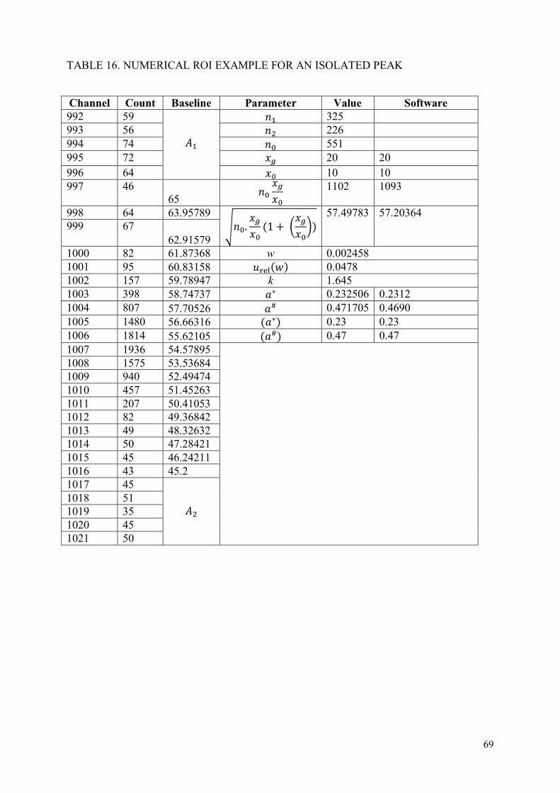
69

TABLE 16. NUMERICAL ROI EXAMPLE FOR AN ISOLATED PEAK

Channel Count Baseline Parameter Value Software

992 59 <�

'� 325 993 56 '5 226 994 74 '& 551 995 72 �% 20 20 996 64 �& 10 10 997 46

65 '& �%�& 1102 1093

998 64 63.95789 ¢'&. �%�& �1 + x�%�&z� 57.49783

57.20364 999 67

62.91579 1000 82 61.87368 w 0.002458 1001 95 60.83158 �é�� 0.0478 1002 157 59.78947 k 1.645 1003 398 58.74737 =∗ 0.232506 0.2312 1004 807 57.70526 =# 0.471705 0.4690 1005 1480 56.66316 �=∗� 0.23 0.23 1006 1814 55.62105 �=#� 0.47 0.47 1007 1936 54.57895 1008 1575 53.53684 1009 940 52.49474 1010 457 51.45263 1011 207 50.41053 1012 82 49.36842 1013 49 48.32632 1014 50 47.28421 1015 45 46.24211 1016 43 45.2 1017 45

<5 1018 51 1019 35 1020 45 1021 50

70

FIG. 16. Example peak used in the simple ROI evaluation for which the data is given in Table 16.

A numerical example for a peak multiplet is given in Table 17 and the related multiplet is represented in Fig. 17. Computations for Α∗and Α#are given here once with and once without considering the overlap of the peaks as an interference contribution to the background of both the considered peaks. A linear baseline model was considered for the complete multiplet region. The approach used here is identical to the one used with the isolated peaks, except for the fact that overlapping ROIs are defined and that the linear background is estimated from the bordering region of the multiplet. The baseline evaluation uses the regionsA�and A5 from which a linear background was computed in the multiplet ROI B. In order to make meaningful comparisons between the results of the software and those computed here, the evaluation of Α∗and Α# for the peaks 1 and 2 (taken from left to right) was based on ROIs B�and B5 as they were defined by the software analysis of this multiplet. The ROIsB�and B5 are indicated in Table 17 by the numbers in the columns B�and B5. For both columns the number 1 indicates the centroid of the peak. For ROI B� a point outside the overall ROI B had to be selected. A comparison of the results for Α∗and Α# reveals a relative difference up to 15% for Α∗and Α#not considering the interference. Further evaluation of the data revealed that the data of the software analysis could be reproduced when '& + �5�'&� = 2. '& is used, hence the software did not account

for the parameter P°Pg.

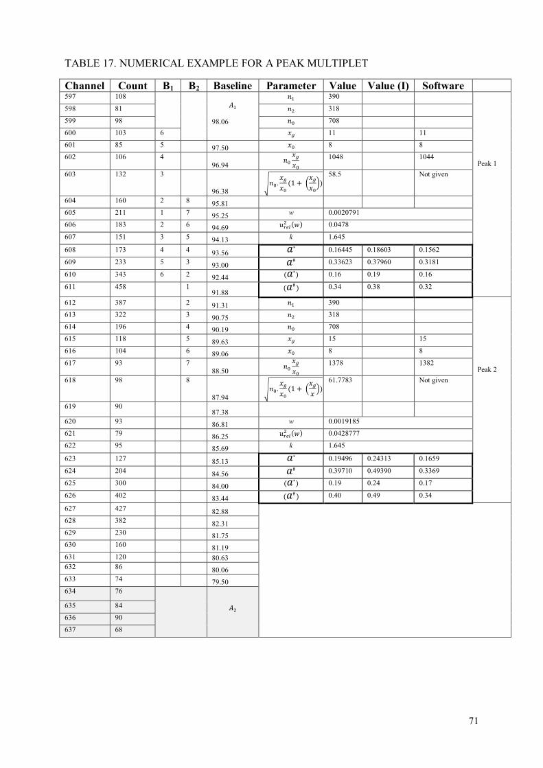
71

TABLE 17. NUMERICAL EXAMPLE FOR A PEAK MULTIPLET

Channel Count B1 B2 Baseline Parameter Value Value (I) Software 597 108 <�

98.06

'� 390 Peak 1

598 81 '5 318

599 98 '& 708

600 103 6 �% 11 11

601 85 5 97.50 �& 8 8

602 106 4 96.94

'& �%�& 1048 1044

603 132 3

96.38 ¢'&. �%�& �1 + x�%�&z�

58.5

Not given

604 160 2 8 95.81

605 211 1 7 95.25 w 0.0020791

606 183 2 6 94.69 ��5 �� 0.0478

607 151 3 5 94.13 k 1.645

608 173 4 4 93.56 =∗ 0.16445 0.18603 0.1562

609 233 5 3 93.00 =# 0.33623 0.37960 0.3181

610 343 6 2 92.44 �=∗� 0.16 0.19 0.16

611 458 1 91.88

�=#� 0.34 0.38 0.32

612 387 2 91.31 '� 390 Peak 2

613 322 3 90.75 '5 318

614 196 4 90.19 '& 708

615 118 5 89.63 �% 15 15

616 104 6 89.06 �& 8 8

617 93 7 88.50

'& �%�& 1378 1382

618 98 8

87.94 ¢'&. �%�& �1 + V�%� W�

61.7783

Not given

619 90 87.38

620 93 86.81 w 0.0019185

621 79 86.25 ��5 �� 0.0428777

622 95 85.69 k 1.645

623 127 85.13 =∗ 0.19496 0.24313 0.1659

624 204 84.56 =# 0.39710 0.49390 0.3369

625 300 84.00 �=∗� 0.19 0.24 0.17

626 402 83.44 �=#� 0.40 0.49 0.34

627 427 82.88

628 382 82.31 629 230 81.75 630 160 81.19 631 120 80.63 632 86 80.06 633 74 79.50 634 76

<5 635 84

636 90

637 68

72

FIG. 17. Multiplet and ROI definitions of which numerical data is represented in Table 17.

To include also the interfering background the following equation was used:

u5�Α� = w5. �n� + n&+u5�n&� S nØSu5�nØ�� S Α5. ül��l (181)

in which 'Øand�5�'Ø� are the counts representing the interference and its variance respectively.

'Ø � �'%Ø . '$Ø� (182)

In which '%Ø represents the gross counts in the peak ROI already corrected for the baseline background, and'$Ø the net counts in the peak (this value is taken from the software that deconvoluted the multiplet).

The variance �5�'Ø� is then obtained as:

�5�'Ø� � V$°Ú_$¬Ú$¬¥

W5

. �5�'$Ö� (183)

The first factor represents the squared ratio of the interfering area to the total net area of the interfering peak. It is assumed to be a constant although strictly it is not since the measure of interference depends also on the counting statistics in both peaks. However since the deconvolution accounted for the counting statistics and the correlations between the data, it is assumed that this uncertainty is already included in �5�'$Ö�, the variance of the interfering peak which is obtained also from the software analysis. Adding these contributions allows accounting for the interference. The results including this correction are given in the column ‘Value (I)’. In this example substantial differences are found between the results computed here and the data obtained from the software analysis. For this case the software cannot be considered as giving results that are ISO 11929:2010 compatible.

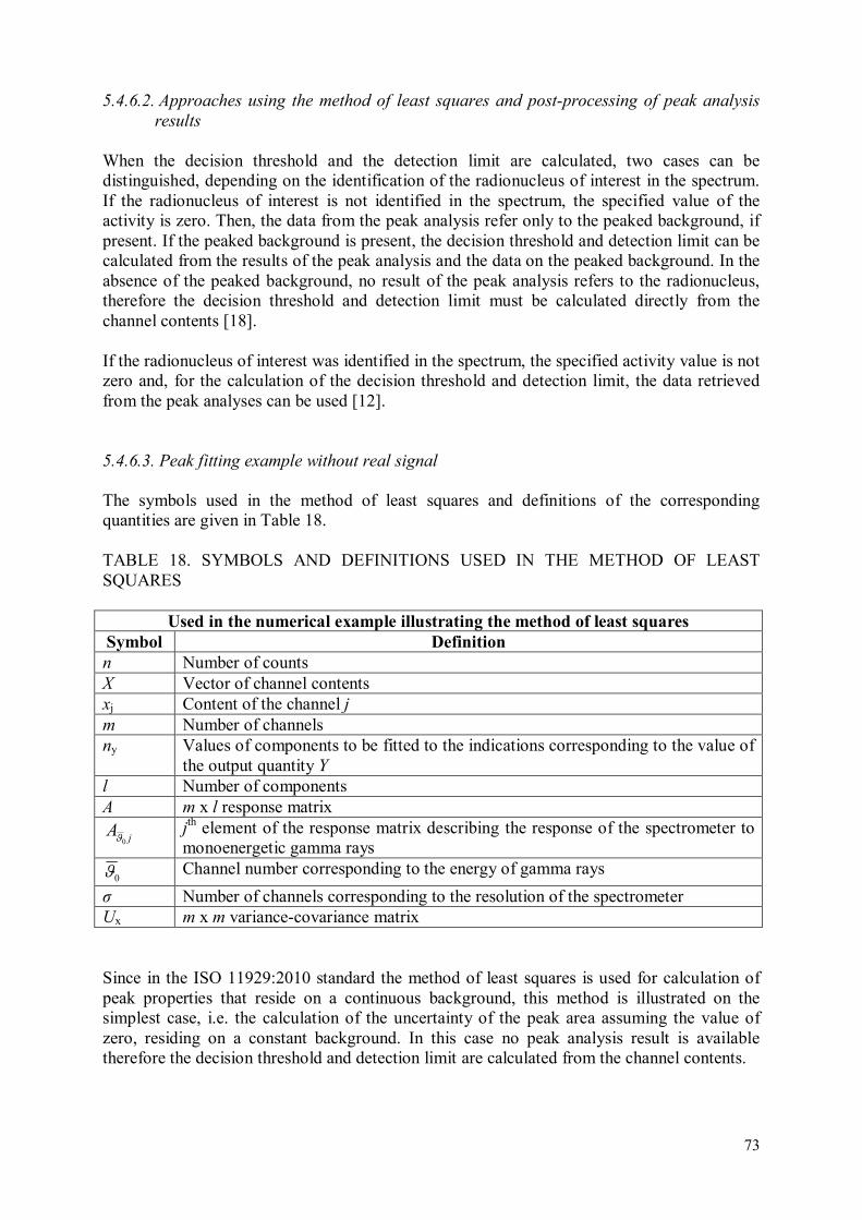
73

5.4.6.2. Approaches using the method of least squares and post-processing of peak analysis

results

When the decision threshold and the detection limit are calculated, two cases can be distinguished, depending on the identification of the radionucleus of interest in the spectrum. If the radionucleus of interest is not identified in the spectrum, the specified value of the activity is zero. Then, the data from the peak analysis refer only to the peaked background, if present. If the peaked background is present, the decision threshold and detection limit can be calculated from the results of the peak analysis and the data on the peaked background. In the absence of the peaked background, no result of the peak analysis refers to the radionucleus, therefore the decision threshold and detection limit must be calculated directly from the channel contents [18]. If the radionucleus of interest was identified in the spectrum, the specified activity value is not zero and, for the calculation of the decision threshold and detection limit, the data retrieved from the peak analyses can be used [12]. 5.4.6.3. Peak fitting example without real signal

The symbols used in the method of least squares and definitions of the corresponding quantities are given in Table 18. TABLE 18. SYMBOLS AND DEFINITIONS USED IN THE METHOD OF LEAST SQUARES

Used in the numerical example illustrating the method of least squares

Symbol Definition

n Number of counts X Vector of channel contents xj Content of the channel j m Number of channels ny Values of components to be fitted to the indications corresponding to the value of

the output quantity Y l Number of components A m x l response matrix

jA

0ϑ j

th element of the response matrix describing the response of the spectrometer to monoenergetic gamma rays

0ϑ Channel number corresponding to the energy of gamma rays

σ Number of channels corresponding to the resolution of the spectrometer Ux m x m variance-covariance matrix Since in the ISO 11929:2010 standard the method of least squares is used for calculation of peak properties that reside on a continuous background, this method is illustrated on the simplest case, i.e. the calculation of the uncertainty of the peak area assuming the value of zero, residing on a constant background. In this case no peak analysis result is available therefore the decision threshold and detection limit are calculated from the channel contents.

74

If the continuous background is constant over an energy range, which is much wider than the FWHM of the peak, the uncertainty of the background height can be determined with a vanishing small uncertainty. In this case, the null measurement uncertainty of the indication (the number of counts) can be easily determined by the method of least squares supposing uncorrelated channel contents with the Poisson probability distribution. In this method, no supposition of the width of the peak region is made, therefore the null measurement uncertainty calculated in this way does not depend on it, the only data needed are the peak position and its width. The least squares method yields the lowest uncertainty of the null indication. The method with the ROI analysis is equivalent to the method of least squares using a uniform peak shape instead of a Gaussian shape. When a spectral region is fitted by the model X = A·nY, where X denotes the vector comprising m channel contents to be fitted, nY the estimates of the l components, nYi to be fitted to the spectrum and A the m x l response matrix. Each column in the matrix with m elements describes the shape, i.e. energy dependence, of one component to be fitted to the spectrum. It should be observed, that, in this calculation, the spectrum X is interpreted as a linear combination of the l components, with the corresponding coefficients nYi. Because the channel contents are uncorrelated and are distributed according to the Poisson distribution, the uncertainty matrix UX is diagonal UX = xi·δij, where i and j assume values in the interval [1, m]. Since only one peak is fitted to a constant continuous background, nY has only one element nY1 and the matrix A comprises only one column describing the response of the spectrometer to mono-energetic gamma-rays. Supposing a Gaussian shape of the response, the matrix elements are:

A ej

j

ϑ

ϑ

σ

πσ0

02

21

22=

−−( )

(184)

where j assumes the values in the interval [-m/2, m/2], and σ is the number of channels corresponding to the FWHM of the response (resolution of the spectrometer):

σ = FWHM E/ ( ln )∆ 8 2 (185)

where ∆E denotes the energy width of one channel. Because there is only one unknown and no peak is present, the peak area with the true value zero has an uncertainty, which can be expressed as:

u nx

eY

j

j

j m

m

22

2

21

1

02

2

01 1

2( )

( )

/

/

= =

−−

=−

−

∑ πσ

ϑσ

(186)

Since the background is constant it can be characterized by its average height, describing the average number of counts in one channel.

75

Because of the normalization, expressing the requirement that the estimate nY1 represents the number of counts, it follows:

e

j

j m

m−

−

=−

=∑( )

/

/ ϑ

σ πσ0

2

22

2

2

2 (187)

or

e

j

j m

m−

−

=−

=∑( )

/

/ ϑ

σ πσ0

2

2

2

2

(188)

Then, the uncertainty simplifies and the indication, corresponding to the decision threshold, can be expressed as:

n k xy* .= −1 12α πσ (189)

The measurement model defining the relation between the indication and the measured quantity value is y = ny·w, where w denotes the conversion factor converting the number of counts to the activity or massic activity. Then, the decision threshold is y* = ny*·w. The detection limit is defined as y

# = y* + k1-β·u(y#), where the uncertainty of the quantity value y# is:

u y u n w n w u wy y rel

2 2 2 2 2 2( ) ( ) ( )## #= +

(190)

In the first approximation for y# its uncertainty u(y#) is evaluated at the indication ny# = 2·ny* [4, p. 11]. Assuming Poisson distribution of channel contents, the uncertainty of the indication u(ny#=2·ny*) is calculated as:

( )u n n ny y

T

y

2 11

2 2( ) ( ) .# * *= = −−

A U AX (191)

Here Ux(2ny*) denotes the uncertainty matrix of channel contents, comprising the sum of the continuous background and the gamma-ray peak with the area of 2·ny* centered at 0ϑ and

having a width of σ. This value has an uncertainty of zero, therefore the matrix Ux(2·ny*) is diagonal. Expressing it with the average channel content, it is:

( )UX ( )* *2 21 0n x n Ay y j ij= + ϑ δ

(192)

and the uncertainty u(ny=2·ny*) becomes:

u n nA

x n Ax

e

n

xe

y y

j

y jj m

m

j

yj

j m

m

2

2

12

21

1

2

1

22

2

1

22

1

2

12 1

2

0

0

02

2

02

2

( ) .**/

/

( )

*( )

/

/

= =+

=

+

=−

− −−

−−

=−

−

∑ ∑ϑ

ϑ

ϑ

σ

ϑ

σ

πσ

πσ (193)

76

The first approximation to the detection limit is then:

y y k u y n ny y1 1 2# #** [ ( )]= + =−β (194)

where u[y#(ny=2·ny*)] denotes the uncertainty of the measurand evaluated at the indication, corresponding to twice the measurement uncertainty:

( )u y n n u n n n u wy y y y y rel

2 2 2 2 22 2 2[ ( )] ( ) ( )#* * *= = = +

(195)

This indication is used in the calculation of the next approximation of y#:

u n xA

n

xA

y

j

y

j

j m

m

21

2

1

2

2

1

2

0

1

01

( ) ,##/

/

=

+

=−

−

∑ ϑ

ϑ

(196)

Then, the uncertainty of the measured quantity is:

( )u y n u n n u w wy y y rel

2 2 2 2 2

2 2 1[ ( )] ( ) ( )#

# # #= + (197)

and the new approximation for the detection limit is:

y y u y ny2

2

# #* [ ( )] .#= + (198)

In this way further approximations of the detection limit can be calculated. 5.4.6.4. Isolated peak, continuous background only

If, besides the isolated peak corresponding to the indication, only the continuous background is present in the peak region and its immediate vicinity, the contribution of the net indication to the spectrum is relatively easy to separate from the background. (a) Constant continuous background, the specified activity value is zero If no peak is present at the energy of interest and its vicinity, no data from the peak analysis is available and, for the calculation of decision threshold and detection limit, the raw spectral data, i.e. the channel contents, must be used. The method can be applied only to cases, where the continuous background is constant in a broad energy range, so that it can be described with one parameter having a negligible uncertainty. Example: Calculation of the detection limit and the decision threshold for the activity concentration of 137Cs

The sample containing V = 0.320 ± 0.001 L of water was placed on a high-resolution gamma detector in a geometry having a counting efficiency of ε = 0.0350 ± 0.0020 at the energy of 662 keV. 137Cs radiates gamma-rays with the energy of 662 keV with an intensity of P = 0.851 ± 0.002. The measurement lasted t = 388,433 s.

77

The activity concentration is calculated as:

wntVP

ny n

n ⋅=⋅⋅⋅

=ε

(199)

And its uncertainty as:

)()()( 222wunnuwyu relnn ⋅+⋅= (200)

where nn denotes the net indication, i.e. the number of counts in the peak. The conversion factor w is given by 1/(P.ε.V.t) and amounts to w = (2.70 ± 0.15)·10-4 s-1.L-1 = 2.70·(1 ± 0.055)·10-4 s-1.L-1.

The spectrum in the vicinity of the energy 662 keV is shown in Fig. 18. The energy width of one channel is 0.337 keV. This spectrum region was used to determine the average height of the channel content x1, which amounts to 37.43 counts per channel. The resolution of the spectrometer at that energy is 1.40 keV, which corresponds to σ = 1.78 channels. The coverage factors used, k1-α = k1-β = 1.645, correspond to the confidence probability 1 - α = 1- β = 95%. The net indication, corresponding to the decision threshold ny*, for this confidence probability is:

n k u ny* ( ) . . . . .= = ⋅ =−1 0 1645 2 178 37 43 25 4α π

The corresponding decision threshold is y* = ny·w = 7.0·10-3 Bq.L-1.

Energy / channels

0 50 100 150 200

Cha

nnel conte

nt

0

20

40

60

80

E= 662 keV

FIG. 18. Spectrum shape in the vicinity of the energy 662 keV. The arrows indicate the limits of the

region where the response functionj

Aϑ differs from zero.

78

The detection limit is calculated from a region that is 2.5 FWHM wide, comprising 11 channels. Using a wider region does not affect the decision threshold and the detection limit since outside 2.5 FWHM the response function is negligible. In this region 99.98% of the peak counts are expected to be registered. Table 19 presents the supposed shape of the spectrometer response and the quantities needed for calculating the first and second approximation to the detection limit, as functions of the channel number j.

TABLE 19. SPECTROMETER RESPONSE TO THE MONOENERGETIC GAMMA-RAYS WITH THE ENERGY OF 662 KEV, AND THE PRODUCTS OF MATRIX ELEMENTS AND uXjj NEEDED FOR THE CALCULATION OF THE DETECTION LIMIT

j ϑ0-j

Ajϑ0

A n A xj y jϑ ϑ0 0

211 2/ ( / )*+

A n A x

j y jϑ ϑ0 1 0

211/ ( / )#+

1 -5 0.00434 0.000019 0.000019

2 -4 0.01796 0.000315 0.000315

3 -3 0.05418 0.002735 0.002723

4 -2 0.11923 0.012238 0.012128

5 -1 0.19137 0.029081 0.028695

6 0 0.22406 0.038511 0.037936

7 1 0.19137 0.029081 0.028695

8 2 0.11923 0.012238 0.012128

9 3 0.05418 0.002735 0.002723

10 4 0.01796 0.000315 0.000315

11 5 0.00434 0.000019 0.000019

Sum 0.9983 0.127289 0.125698

From Table 19 it follows:

A

n

xA

u nx

n n n u n

j

y

j

jy

y y y y

ϑ

ϑ

0

0

2

1

5

5

21

2

12 012729

0127291715

2 1645 537

+= = =

= + =

=−∑

**

* * *

. ( ).

.

( ) . ( ) .#

The calculated net indications, corresponding to the decision threshold and to the detection limit, correspond to the Currie’s critical level and detection limit LC = 25.3 and LD = 53.4 respectively, using a width of the peak region, which is 1.5 FWHM wide [19].

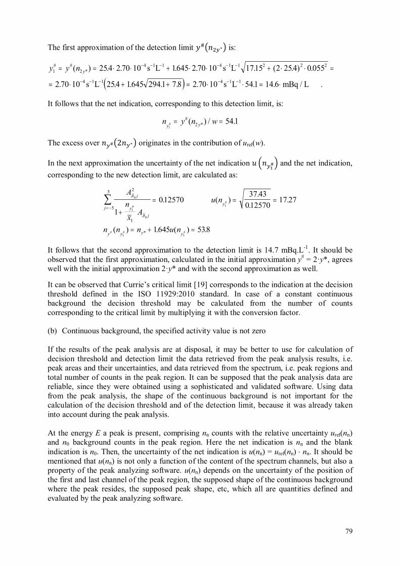
79

The first approximation of the detection limit �#:'5\∗; is:

( )y y n y1 2

4 4 2 2 2

4 4

254 2 70 10 1645 2 70 10 1715 2 254 0 055

2 70 10 254 1645 2941 7 8 2 70 10 541 14 6

# #*( ) . . . . . ( . ) .

. . . . . . . .

= = ⋅ ⋅ + ⋅ ⋅ + ⋅ ⋅ =

= ⋅ + + = ⋅ ⋅ = ⋅

− − − − − −

− − − − − −

s L s L

s L s L mBq / L .

1 1 1 1

1 1 1 1

It follows that the net indication, corresponding to this detection limit, is:

n y n wy y

12 541#

#*( ) / .= =

The excess over '\#:2'\∗; originates in the contribution of urel(w).

In the next approximation the uncertainty of the net indication � V'\¡#W and the net indication,

corresponding to the new detection limit, are calculated as:

A

n

xA

u n

n n n u n

j

y

j

jy

y y y y

ϑ

ϑ

0

1

0

1

1 1

2

1

5

5

1

01257037 43

01257017 27

1645 538

+

= = =

= + =

=−∑

##

# # #

. ( ).

..

( ) . ( ) .*

It follows that the second approximation to the detection limit is 14.7 mBq.L-1. It should be observed that the first approximation, calculated in the initial approximation y# = 2·y*, agrees well with the initial approximation 2·y* and with the second approximation as well.

It can be observed that Currie’s critical limit [19] corresponds to the indication at the decision threshold defined in the ISO 11929:2010 standard. In case of a constant continuous background the decision threshold may be calculated from the number of counts corresponding to the critical limit by multiplying it with the conversion factor.

(b) Continuous background, the specified activity value is not zero If the results of the peak analysis are at disposal, it may be better to use for calculation of decision threshold and detection limit the data retrieved from the peak analysis results, i.e. peak areas and their uncertainties, and data retrieved from the spectrum, i.e. peak regions and total number of counts in the peak region. It can be supposed that the peak analysis data are reliable, since they were obtained using a sophisticated and validated software. Using data from the peak analysis, the shape of the continuous background is not important for the calculation of the decision threshold and of the detection limit, because it was already taken into account during the peak analysis. At the energy E a peak is present, comprising nn counts with the relative uncertainty urel(nn) and n0 background counts in the peak region. Here the net indication is nn and the blank indication is n0. Then, the uncertainty of the net indication is u(nn) = urel(nn) · nn. It should be mentioned that u(nn) is not only a function of the content of the spectrum channels, but also a property of the peak analyzing software. u(nn) depends on the uncertainty of the position of the first and last channel of the peak region, the supposed shape of the continuous background where the peak resides, the supposed peak shape, etc, which all are quantities defined and evaluated by the peak analyzing software.

80

The uncertainty of the total number of counts in the peak region is u2(ng) = ng. Because the uncertainty of the blank indication is the null measurement uncertainty of the indicating quantity, the decision threshold of the measurand, calculated by the measurement model y = nn·w, expressed with the data retrieved from the peak analysis report, is:

wnukwny ny ⋅=⋅=⋅= − )0(* 1* α (201)

where ny* denotes the net indication corresponding to the decision threshold. If sources of measurement bias, i.e. peaked background, are present, the uncertainty of the blank indication is:

)()0()0( 222BnnB nununu +=== (202)

where u(nn=0) denotes the uncertainty of the blank indication if the uncertainty of the peaked background is zero and u(nB) the uncertainty of the peaked background respectively. The detection limit is given by y# = y* + k1-β·u(y#), where:

)()()( 22222#2## wuwnnuwyu relyy

⋅⋅+⋅= (203)

Here ny# and u(ny#) denote the net indication and its uncertainty, respectively, when the specified activity value of the measurand is y#. In the absence of the peaked background for isolated peaks the uncertainty of the net indication u(ny#) is calculated from the equation u(n0) = u(np) - u(ng). Then it follows that u(ny#) = u(n0) + u(ngy#), where ngy# denotes the total number of counts in the peak region, if the peak area amounts to ny# counts for u2(ngy#) = n0 + ny#. The first approximation of u(ny#) is calculated by the initial approximation y# = 2·y*, i.e. ny# = 2·ny*. Then:

*# 2)()( 00 yynnnunu ⋅++= (204)

and in the first approximation the detection limit is expressed as:

[ ] )()2(2)(645.1* 22*

2

*001#1 wunnnnuwkyy relyy ⋅⋅+⋅++⋅⋅⋅+= −α (205)

The net indication, that corresponds to this decision threshold, is ny#1=y#1/w and the next approximation to the detection limit is obtained by substituting ny#1 instead of 2·ny* into the expression for the detection limit. Example: Calculation of the decision threshold and of the detection limit for the massic activity of 137Cs in a soil sample A sample containing m = 0.4307 ± 0.0001 kg of soil with a density of 1.27 kg.L-1 was placed on a high-purity germanium gamma detector in a geometry with a counting efficiency of ε = 0.00901 ± 0.00035 at the energy of 662 keV. 137Cs radiates at the energy of 662 keV with the intensity of P = 0.851 ± 0.002. The measurement lasted t = 79,528 s.

81

The massic activity is calculated as:

wntmp

ny n

n ⋅=⋅⋅⋅

=ε

(206)

where the conversion factor has a value of w = (3.81 ± 0.15)·10-3 s-1.kg-1 = 3.81·(1 ± 0.039)·10-3 s-1.kg-1. The decision threshold and the detection limit are calculated with the coverage factors k1-α = k1-β = 1.645, corresponding to the probabilities for the errors of the first and second kind α = β = 0.05. The spectrum in the vicinity of the energy 662 keV is shown in Fig. 19.

Channel number

20 40 60 80

Ch

an

nel co

nte

nt

0

50

100

150

200

250E = 662 keV

E =665 keV

FIG. 19. Spectrum in the vicinity of the energy 662 keV.

The energy width of one channel is 0.349 keV. The data retrieved from the peak analysis are: np = 911 and urel(np) = 0.078 from where it follows u(np) = 71. The total number of counts in the peak region is ng = 1475 having an uncertainty of u(ng) = 38. It follows that the number of counts in the background is n0 = 564. Since no peaked background appears, nn = np. It can be observed that, at the energy of 665 keV, a small peak is present, which can affect the calculation of the null measurement uncertainty by the ROI analysis or by supposing a constant background, when calculated directly from channel contents. However, since the peaks do not overlap, the peak analysis program does not classify the peaks as overlapping, therefore the presence of the peak at 665 keV does not affect the results of the peak analysis referring to the peak at 662 keV. It follows that, when using peak analysis results, the presence of this peak has no influence on the decision threshold.

82

The uncertainty of the number of counts in the continuous background is u(n0) = u(np) – u(ng)= 71–14751/2=33. For the uncertainty of the blank indication, the

equation pggpn nnnnunu −+−== )()0( is used, from where u(nn=0) is evaluated as

u(nn=0) = 71–14751/2+(1475-911)1/2=57 and the net indication at the decision threshold is ny* = 1.645⋅57 = 94. The decision threshold itself is y* = 1.645⋅57⋅3.81·10-3 Bq.kg-1 = 0.36 Bq.kg-1. The detection limit is calculated using for initial approximation the net indication ny# = 2·ny*. Then, the uncertainty of this indication is:

=⋅++−=⋅++= *0*00 2)(2)()( # ygpynnnnnunnnunu 71 – 14751/2 + (564+2·94)1/2 = 60.

The uncertainty of the corresponding specified quantity value is:

1-1-3

-1223222#

Bq.kg23.0Bq.kg601081.3

Bq.kg)039.0942(601081.3)()()( ##

=⋅⋅

=⋅⋅+⋅=⋅+=

−

−wunnuwyu relyy

which corresponds to the net indication u(ny#) = 60. In the first approximation the detection limit is y# = 1.645⋅w[u(nn=0) + u(ny#)] = 1.645⋅3.81⋅10-3·(57 + 60) Bq.kg-1 = 0.73 Bq.kg-1. The net indication corresponding to this detection limit is ny#1 =1.645·(57+60) = 192 and its uncertainty u(ny#) = u(n0) + (n0 + ny#1)

1/2 = 33+(564+192)1/2= 60. Since this uncertainty coincides with the uncertainty of the net indication calculated with the initial approximation, a further step in the iteration is not necessary and the detection limit is assessed to be y# = 0.73 Bq.kg-1.

5.4.6.5. Continuous background, the specified activity of the value is not zero, there are

overlapping peaks

When, besides the continuous background, also overlapping peaks are present, the net indication, i.e. the peak area, which is due to the radionuclide of interest, must be separated from the background. This separation can be performed by the peak analysis or not, depending on the spectrometer resolution and the difference between the energy of the peak, representing the overlapping peak or the peaked background, and the energy where the gamma-ray emitter of interest radiates. If the specified activity value of the radionuclide of interest is not zero, the ability to separate the net indication from the blank indication, i.e. the background, is given also by the ratio of the net indication and the number of counts of the neighboring peak in the peak region. Depending on the degree to which the peak analysis can separate both contributions various circumstances may occur. When peaks overlap strongly, the peak analysis software calculates the FWHMs of the overlapping peaks simultaneously with their areas by the non-linear method of least squares. Therefore the peak areas calculated may not correspond to the FWHMs from the spectrometer FWHM calibration. It is therefore safer to extend the peak region over both peaks.

83

When peaks overlap, besides the continuous background also the counts of the overlapping peak present a contribution to the background. Therefore it is necessary to retrieve the total number of counts in the peak region from the number of counts in a ROI comprising the peak presenting the net indication. Then, the number of background counts is calculated by subtracting the indication from the total number of counts. Usually, the ROI is 2.5 FWHM wide, but in the case when peaks overlap strongly, it may be better to include the overlapping peak into the peak region. When peaks overlap, various degrees of overlapping may occur. The following numerical examples are aimed to present cases with different degrees of overlapping, from the case when the peak analysis can decompose the overlapping peaks to the case when the decomposition is not possible. The extreme case presents the peaked background, when the data on the blank indication must be retrieved from separate measurements, e.g. background measurements. When peaks overlap, the uncertainty of their area is not given only by the Poisson distribution of the channel contents but also by the conditioning of the system of equations, which is used for the decomposition of the composed peak into its components. Therefore here the uncertainty u(np) may be much larger than ng

1/2. Example: Calculation of the decision threshold and of the detection limit for the activity concentration of 65Zn A sample containing 0.4931 ± 0.0001 kg of soil with a density of 1.27 kg.L-1 was placed on a high-purity germanium gamma detector in a geometry with the counting efficiency of 0.600% ± 0.0024% at the energy of 1,115 keV. The indication corresponding to 65Zn was obtained by counting a 65Zn source simultaneously with a soil sample. 65Zn radiates at 1,115 keV with the intensity of 50.60% ± 0.24%. The measurement lasted 22,699 s. The decision threshold and the detection limit are calculated with the coverage factors k1-α = k1-β = 1.645, corresponding to the probabilities for the errors of the first and second kind α = β = 0.05. Because of the presence of 226Ra in the soil, a peak occurs at the energy of 1,120 keV, belonging to the decay of the radon daughter 214Bi. This peak overlaps partially with the peak belonging to 65Zn. The massic activity is calculated as:

tmp

ny n

⋅⋅⋅=

ε (207)

where the conversion factor has a value of w = (29.4 ± 1.2)·10-3 s-1.kg-1 = 29.43·(1 ± 0.040)·10-3 s-1.kg-1. The spectrum in the vicinity of the energy 1,115 keV is shown in Fig. 20. The energy width of one channel is 0.331 keV. The resolution at the energy 1,115 keV is 2.04 keV. The data retrieved from the peak analysis are: np = 389,735 and urel(np) = 0.019. It follows that u(np) = 7,405. Since no peaked background occurs, nn= np. It can be observed in Fig. 20 that, at the energy of 1,120 keV, a strong peak occurs which affects the background under the peak belonging to 65Zn. Here the number of counts of the continuous background does not describe the background under the peak, because besides the continuous background also the tail of the peak at 1,120 keV contributes to the background.

84

Therefore an energy interval, indicated in Fig. 20 and comprising a large fraction of the counts in the peak at 1,115 keV, is used for the determination of the background. The interval comprises ng = 466,388 counts. Then, the number of background counts is n0 = ng – np = 466,388 – 389,735 = 76,653.

Channel number

20 40 60 80

Cha

nn

el con

ten

t

0

20000

40000

60000

80000

E = 1115 keV

E = 1120 keV

FIG. 20. Spectrum in the vicinity of the energy 1,115 keV.

Because peaks overlap, the equation gn nnunu += )()( 0 is used for calculating the

uncertainty of the number of counts in the background, from where u(n0) = 7,405+683 = 8,088 and the uncertainty of the blank indication is:

811,7)735,389388,466(088,8)()0( 2/10 =−−=−−== ngn nnnunu .

Then, the net indication corresponding to the decision threshold is: ny* = 1.645·7,811 = 12,849. The decision threshold itself is: y* = 12,849·29.43·10-3 s-1.kg-1 = 378 Bq.kg-1. The detection limit y# is calculated with the initial approximation for its net indication, i.e. the

net number of counts, ny# = 2·12,849 = 25,698. Because the equation gn nnunu += )()( 0 is

used for calculating the uncertainty of the number of counts in the background, it follows that

## 2)()( 00 yynnnunu ⋅+−= = 8,088-(76,653+25,698)1/2 = 7,768.

85

The uncertainty of the corresponding specified quantity value u(2·y*) is:

1-1-3-

-1223222#

Bq.kg231Bq.kg836,71029.43

Bq.kg)040.0698,25(77681043.29)()()( ##

=⋅⋅

=⋅+⋅⋅=⋅+⋅= −wunnuwyu relyy

which corresponds to the net indication u(ny#) = 7,836. In the first approximation the detection limit is y

# = 1.645⋅w[u(nn=0) + u(ny#)] = 1.645⋅29.43⋅10-3·(7,811+7,836) Bq.kg-1 = 758 Bq.kg-1. The net indication corresponding to this detection limit is ny#1 = 25,839 and its uncertainty is u(ny#1) = u(n0) - (n0 + ny#1)

1/2 = 8,088-(76,653+25,839)1/2 = 7,768. Since this uncertainty coincides with the uncertainty u(2·ny*) = 7,768, a further step in the iteration is not necessary and the detection limit is assessed to be y# = 753 Bq.kg-1. Example: Calculation of the decision threshold and of the detection limit for the activity concentration of 88Y As an example for calculation of decision threshold and detection limit when the peak belonging to the radionuclide of interest overlaps strongly with another peak, but the peak analyzing software can still separate both peaks, the decision threshold and detection limit of 88Y are calculated from the peak at the energy of 1,836 keV. Simultaneously with the sample containing 88Y, a source containing 226Ra was counted to provide for the interfering peak. The interfering peak occurs at 1,838 keV and belongs to the decay of the radon daughter 214Bi. A sample containing 0.241 ± 0.01 L of 88Y water solution with a density of 1.01 kg.L-1 was counted on a high-purity germanium gamma detector in a geometry with a counting efficiency of ε = 0.468% ± 0.016% at the energy of 1,836 keV. 88Y radiates at this energy with the probability of 99.36% ± 0.03%. The measurement lasted 55,430 s. The decision threshold and the detection limit are calculated with the coverage factors k1-α = k1-β = 1.645, corresponding to the probabilities for the errors of the first and second kind α = β = 0.05. Since no peaked background is present nn = np. The activity concentration is calculated as:

tVP

ny n

⋅⋅⋅=

ε (208)

where the conversion factor assumes a value of w = (16.39 ± 0.56)·10-3 L-1.s-1 = 16.39·(1 ± 0.034)·10-3 L-1.s-1. The spectrum in the vicinity of the energy 1,836 keV is shown in Fig. 21.

86

Channel number

10 20 30 40 50

Cha

nn

el con

ten

t

0

1000

2000

3000

4000

5000

6000

E = 1836 keV E = 1838 keV


The resolution at this energy is 2.42 keV. The energy width of one channel is 0.331 keV. The data retrieved from the peak analysis are np = 22,064 and urel(np) = 0.086, from what u(np) = 1,898. The region of interest is indicated in Fig. 21, from where ng =78,684 is obtained. Since the FWHM of the peak at 1,836 keV may not be equal to the FWHM calculated from the FWHM calibration of the spectrometer, the peak region extends over both peaks. The number of counts in the background, i.e. the blank indication, is then n0 = 78,684–22,064 = 56,620. Since peaks overlap, the equation u(n0) = u(np) + u(ng) is used for calculating the uncertainty of the number of counts in the background u(n0) = 1,898 + 281 = 2,179. The uncertainty of the blank indication is:

pgn nnnunu −−== )()0( 0 941,1)064,22684,78(179,2 2/1 =−−=

The net indication corresponding to the decision threshold is ny* = 1.645·1,941 = 3,193 and the decision threshold itself is 3,193·16.39·10-3 Bq.L-1 = 52.3 Bq.L-1. The detection limit is calculated with the initial approximation for the net indication ny# = 2·ny*, from where u(ny#) = u(n0) - (n0 + 2·ny*)

1/2 = 2,179 - (56,620 + 2·3,193)1/2 = 1,928

87

The uncertainty of the specified quantity value, y#(2·ny*), is:

1-1-3-

-1223222#

Bq.kg 31.8Bq.kg940,11016.39

Bq.kg)034.0193,32(928,11039.16)()()( ##

=⋅⋅

=⋅⋅+⋅⋅=⋅+⋅= −wunnuwyu relyy

This uncertainty corresponds to the uncertainty of the net indication u(ny#) = 1,940. In the first approximation the detection limit is y

# = 1.645⋅w[u(nn=0) + u(ny#)] = 1.645⋅16.39⋅10-3

· (1,941 + 1,940) Bq.L-1 = 104.6 Bq.L-1. The net indication corresponding to this detection limit is ny#1 = 1.645·(1,941 + 1,940) = 6,384 and its uncertainty is u(ny#1) = u(n0) - (n0 + ny#1)

1/2 = 2,179-(56,620+ 6,384)1/2 = 1,928. Since this uncertainty coincides with the uncertainty calculated with the initial approximation, a further step in the iteration is not necessary and the detection limit can be assessed to be y# = 104.6 Bq.L-1. Example: Calculation of the decision threshold and of the detection limit for the massic activity of 88Y

As an example for calculation of the decision threshold and of the detection limit in the case of strongly overlapping peaks, the calculation for 88Y is presented. This corresponds to the case for which the peak belonging to the radionuclide of interest is much smaller than the interfering peak, but the peak analysis still separates both peaks. A sample containing 10.0 ± 0.1 g of 88Y water solution with a density of 1.01 g.cm-3 was measured on a high-purity germanium gamma detector in a geometry having a counting efficiency of ε = 1.22% ± 0.13% at the energy of 1,836 keV. At this energy 88Y radiates with the intensity of 99.36% ± 0.03%. The acquisition time is 55,586 s. The decision threshold and the detection limit are calculated with the coverage factors k1-α = k1-β = 1.645, corresponding to the probabilities for the errors of the first and second kind α = β = 0.05. Simultaneously with the sample containing 88Y, a source containing 226Ra was counted to provide for the interfering peak. Since no peaked background is present, np = nn. The interfering peak occurs at 1,838 keV and belongs to the decay of the radon daughter 214Bi. The massic activity is calculated as:

tmp

ny n

⋅⋅⋅=

ε (209)

where the conversion factor has a value of w = (0.1484 ± 0.016)·10-3 g-1.s-1 = 0.1484·(1 ±. 0.106)·10-3 g-1.s-1. The spectrum in the vicinity of the energy 1,836 keV is shown in Fig. 22.

88

Channel number

10 20 30 40 50

Cha

nn

el con

ten

t

0

1000

2000

3000

4000

5000

E = 1836 keVE = 1838 keV


The resolution of the spectrometer at this energy is 2.42 keV, the energy width of one channel is 0.331 keV. The data retrieved from the peak analysis are np = 6,951 and urel(np) = 0.054. From these data u(np) = 375. The total number of counts in the region of the peak of interest is obtained from the total number of counts in the spectral region comprising both overlapping peaks. In the spectral region indicated in Fig. 22, the total number of counts obtained is ng= 57,479. The total number of counts in the background, i. e. the blank indication, is n0 = 57,479–6,951 = 50,528. Since peaks overlap, the equation u(n0) = u(np) + u(ng) is used for calculating the uncertainty of the number of counts in the background, therefore u(n0) = 375+240 = 615. The uncertainty of the blank indication is:

pgn nnnunu −−== )()0( 0 = 615–(57,479–6,951)1/2 = 390.

The indication corresponding to the decision threshold is ny* = 1.645·390 = 642 and the decision threshold is y* = 642·0.1484·10-3 Bq.g-1 = 0.0953 Bq.g-1. The detection limit is calculated with the initial approximation for the net indication ny# = 2·ny*, from where u(ny#) = u(n0) - (n0 + 2·ny*)

1/2 = 615 – (50,528 + 2·642)1/2 = 387. The uncertainty of the specified quantity value y#(2·ny*) is:

1-1-3-

-1223222#

Bq.g 6090.0Bq.kg410100.1484

Bq.g)106.06422(387101484.0)()()( ##

=⋅⋅

=⋅⋅+⋅⋅=⋅+⋅= −wunnuwyu relyy

89

This uncertainty corresponds to the uncertainty of the net indication u(ny#) = 410. In the first approximation the detection limit is:

y# = 1.645⋅w[u(nn=0) + u(ny#)] = 1.645⋅0.1484⋅10-3(390+410) Bq.g-1 = 0.195 Bq.g-1.

The net indication corresponding to this detection limit is ny#1 = 1.645·(390+410) = 1,316 and its uncertainty is u(ny#1) = u(n0) -(n0 + ny#1)

1/2 = 615-(50,528+1,316)1/2 = 387. Since this uncertainty coincides with the uncertainty calculated with the initial approximation, a further step in the iteration is not necessary and the detection limit can be assessed to be y

# = 0.195 Bq.g-1.

5.4.6.6. Continuous and peaked background

When peaked background is present, not all counts in the peak belong to the signal from the sample but some also to the peaked background, which represents the measurement bias. The number of counts in the peak is therefore np = nn + nB, where np represents the total number of counts in the peak and nB the number of counts in the peaked background respectively. Therefore two components contribute to the uncertainty of the blank indication: the component belonging to the number of counts in the peak when the uncertainty of the number of background counts is zero, u(nn=0), and the component belonging to the uncertainty of the measurement bias u(nB). Because the value of the bias is obtained from separate measurements when it originates in the spectrometer background or the contribution of the blank sample, or from other peaks in the spectrum, if it originates in spectral interferences, it is statistically independent from the number of counts reported by the peak analysis. Therefore the uncertainty of the blank indication is calculated as:

)()0()0( 222BnnB nununu +=== (210)

In the presence of sources of measurement bias, for isolated peaks, u(nn=0) is calculated as:

)()()()0( 00 Bpggpgn nnnnnunnunu −−+−=+== (211)

Where np denotes the number of counts in the peak, which is retrieved from the peak analysis and ng0 = ng - nn denotes the total number of counts in the peak region if the indication is zero. In the case of nB = 0 and u(nB) = 0, it follows that np = nn and the expression for uB(nn=0) reduces to the expression for u(nn=0). On the other hand, in the absence of continuous

background, i.e. n0 = 0 and u(n0) = 0, at nn = 0, it follows that np = nB = ng and gp nnu ≈)( .

The uncertainty of the net indication is then gn nnu == )0( .

In case of overlapping peaks, u(nn=0) is calculated as:

)()()()0( 00 Bpggpgn nnnnnunnunu −−−+=−== (212)

When n0 << np and u(n0) ≈ 0, then nn = 0, it follows that np = nB ≈ ng and gp nnu ≈)(

The uncertainty of the vanishing net indication is then gggn nnnnu =−⋅== 2)0(

90

Example: Calculation of the decision threshold and of the detection limit in the presence of background, case of 40K activity concentration When the net indication corresponding to the radionuclide of interest already appears in the spectrometer background, the background count rate and its uncertainty cannot be obtained from the measured spectrum, as in the case of interference correction, but must be retrieved from separate measurements, i.e. background measurements. Then, the uncertainty of the blank indication originates in two sources, i.e. in the spectrum measurement and in the background measurement. A sample of dry residue, obtained with evaporation of 0.04603 m3 ± 0.00002 m3 of water, was counted on a high-purity germanium gamma detector in a geometry with the counting efficiency of 0.0147 ± 0.0014 at 1461 keV. At this energy gamma-rays originating in the decay of 40K are emitted with the intensity of 0.1067 ± 0.0011. The measurement lasted 299,300 s. The decision threshold and the detection limit are calculated with the coverage factors k1-α = k1-β = 1.645, corresponding to the probabilities for the errors of the first and second kind α = β = 0.05. The activity concentration is calculated as:

tmp

ny n

⋅⋅⋅=

ε (213)

where the conversion factor has a value of w = (46.28 ± 4.44)·10-3 m-3.s-1 = 46.28·(1 ± 0.096)·10-3 m-3.s-1. The peaked background count rate at the energy of 1,461 keV amounts to 0.00240 s-1 ± 0.00019 s-1, which corresponds to the background peak area in the spectrum nB = 717 and its uncertainty u(nB) = 57. The data retrieved from the peak analysis, i.e. the number of counts in the peak at 1,461 keV, is np = 1099 and its relative uncertainty is urel(np) = 0.042. The uncertainty of the number of counts in the peak is u(np) = 46. The total number of counts in the peak region is ng = 1,227, its uncertainty is u(ng) = 35. The number of counts due to the indication is nn = np – nB = 1,099–717 = 382. The uncertainty of the blank indication due to the peak is: u(nn=0) = 46–35+[1,227–(1,099–717)]1/2 = 40.

The total uncertainty of the blank indication is uB(nn=0) = (402 + 572)1/2 = 70. The net indication corresponding to the decision threshold is ny* = 1.645·70 = 115 and the decision threshold is y* = wny* = 46.28·10-3·115 Bq.m-3 = 5.3 Bq.m-3.

The detection limit is calculated with the initial approximation for the net indication ny# = 2·ny*, from where u(ny#) is:

[ ] =+⋅+−−+−=+= )(2)()()()()( 22

*222

## ByBpggpByyB nunnnnnnunununu

= {46 – 35 + [1,227 – (1,099 – 717) + 2·115]1/2}2 + 572 = (46 – 35 + 33)2 + 572 = 442 + 572 =

= 5,166,

and uB(ny#) = 72 follows.

91

The corresponding uncertainty of the specified quantity value, y(2·ny*) is:

=⋅⋅+⋅⋅=⋅+⋅= − -3223222# Bq.m)096.01152(721028.46)()()( ## wunnuwyu relyyB

46.28·10-3·75 Bq.m-3 = 3.49 Bq.m-3. This uncertainty corresponds to the uncertainty of the net indication u(ny#) = 75. In the first approximation, the detection limit is: y# = 1.645⋅w[uB(nn=0) + u(ny#)] = 1.645⋅46.28⋅10-3·(70+75) Bq.m-3 = 11.04 Bq.m-3. The net indication corresponding to this detection limit is ny#1 = 1.645·(70 +75) = 238 and its uncertainty is:

[ ] =++−−+−=+= )()()()()()( 22222#1

##1

ByBpggpByyB nunnnnnnunununu

= {46 – 35 + [1,227 – (1,099 – 717) +238]1/2}2 + 572 = (46 – 35 + 33)2 + 572 = 442 + 572 = 5,166.

Since this uncertainty coincides with the uncertainty calculated with the initial approximation, a further step in the iteration is not necessary and the detection limit can be assessed to be y

# = 11.04 Bq.kg-1. Example: Calculation of the decision threshold and of the detection limit in the presence of interference, case of massic activity of 109Cd in soil As an example for calculation of the decision threshold and of the detection limit in case the peak analysis procedure cannot decompose a peak in the spectrum to its overlapping components, the case of 109Cd in soil is presented. The gamma-ray peak of 109Cd with the energy of 88.0 keV overlaps with the peak due to bismuth Kβ1 X-rays at the energy 87.2 keV, generated in the decay of 214Pb. A sample containing 0.8702 ± 0.0001 kg of soil was counted on a high-purity germanium gamma-ray detector in a geometry with the counting efficiency of 3.70% ± 0.21% at the energy of 88 keV. 109Cd emits gamma-rays at this energy with the intensity of 3.63% ± 0.02%. Simultaneously with the soil sample also a 109Cd source was counted in order to provide the indication for the 109Cd activity. The measurement lasted 51,350 s. The decision threshold and the detection limit are calculated with the coverage factors k1-α = k1-β = 1.645, corresponding to the probabilities for the errors of the first and second kind α = β = 0.05. The massic activity is calculated as:

tmp

ny n

⋅⋅⋅=

ε (214)

where the conversion factor has a value of w = (16.66 ± 0.95)·10-3 kg-1.s-1 = 16.66·(1 ± 0.057)·10-3 kg-1.s-1.

The spectrum near the energy 88 keV is shown in Fig. 23. The resolution at this energy is 1.3 keV. The energy width of one channel is 0.331 keV.

92

Channel number

20 40 60 80

Cha

nn

el con

ten

t

0

1x106

2x106

3x106

EKβ1

+Eγ109Cd = 87.2 keV+88.0 keV

EKβ2

= 90.1 keV

EKα2

= 74.8 keV

EKα1

= 77.1 keV

FIG. 23. Spectrum in the vicinity of the energy 88.0 keV.

Since the peak analysis cannot decompose the peak at 88 keV into its components, the number of background counts must be obtained from the number of counts in the ROI region comprising both overlapping peaks, i.e. the number of counts in the channels 53–62, and the number of counts belonging to the Kβ1 X-rays. This number can be estimated from the number of other X-ray peaks, since they originate from the same source. The data on these peaks are presented in Table 20. TABLE 20. DATA ON THE X-RAY PEAKS AND THE NUMBER OF COUNTS BELONGING TO THE Kβ1 X-RAYS CALCULATED FROM DIFFERENT X-RAY PEAKS Energy /

keV Intensity P(E) Counting

efficiency

ε(E)

Number of counts n(E)

Number of counts

n(EKβ1)

74.8 0.0652 ± 0.0033 0.0352 ± 0.0020 4566044 ± 319623 2857010 ± 347233

77.1 0.110 ± 0.006 0.0359 ± 0.0021 8392607 ± 318301 3051857 ± 315191

90.1 0.0115 ± 0.0006 0.0371 ± 0.0020 1054105 ± 141250 3544953 ± 588437

93

From each of these peaks the number of counts belonging to the Kβ1 X-rays can be calculated as:

)()()(

)()(11

1En

EEP

EEPn

KK

K ⋅⋅

⋅=

ε

εββ

β (215)

where p(EKβ1) = 0.0388 ± 0.0020 and ε(EKβ1) = 0.0370 ± 0.0021 denote the intensity and the efficiency for the Kβ1 X-rays.

In the last column of Table 20 the number of counts belonging to the Kβ1 X-rays is given, calculated separately from other X-ray peaks. The estimated number of Kβ1 X-ray counts is obtained as the weighted mean of these counts, disregarding correlations among intensities, efficiencies and numbers of counts, because these peaks do not overlap. It is

1βKB nn = = 3,042,928 with the uncertainty u( nKβ1) = 216,800.

The number of counts in the channels 53–62 is ng = 6,012,583 with the uncertainty u(ng) = 6,012,5831/2 = 2,452. The total number of counts in the composite peak is retrieved from the peak analysis data np,88 = 4,460,007 with the uncertainty u(np,88) = 258,680. It follows then that the net indication, i.e. the number of counts belonging to the gamma-rays of 109Cd, is nn = np,88 - nKβ1

= 1,417,079.

Because the peak at 88 keV does not overlap strongly with the interfering peaks (except with the peak at 90.1 keV), its area is assumed to be statistically independent from the mean

1βKn .

Therefore the variance of the number of counts belonging to the 109Cd gamma-rays is the sum of the variances of the counts in the peak and the interfering counts u(nn) = [u(np,88)

2 + u( nKβ1)2]1/2 =[258,6802 + 216,8002]= 337,517. The number of counts in the

continuous background counts is then n0 = ng – np,88 = 1,552,576. Since the peak at 88.0 keV overlaps with the peak at 90.1 keV, the equation u(n0) = u(np,88) + u(ng) is used for calculating the uncertainty of the background counts, from where u(n0) = 258,680 + 2,452 = 261,132 follows. The uncertainty of the blank indication in case of a vanishing uncertainty of the measurement bias is:

)()()0(188,0 βKpgn nnnnunu −−−== = 261,132 – (6,012,583 – 1,417,079)1/2 = 258,988.

Taking into account the non-vanishing uncertainty of the measurement bias, the uncertainty of

the blank becomes )()0()0(1

222

βKnnB nununu +=== = 258,9882 + 216,8002 = 337,7532.

The indication corresponding to the decision threshold is then ny* = 1.645·337,753 = 555,603 and the decision threshold is y* = ny*w = 9,256 Bq.kg-1.

94

The detection limit is calculated with the initial approximation for the net indication ny# = 2·ny*, the uncertainty of the indication, )( #

1 yn nuKβ

is:

[ ][ ]

.565,337800,216)389,2132,261(

800,216603,5552)928,042,3007,460,4(583,012,6452,2680,258

)(2)()()()()(

222

22

22

*222

111##

1

=+−

=+⋅+−−−+

=++−−−+=+=ββββ kyKpggpKyyn nunnnnnnunununu

K

The corresponding uncertainty of the specified value y(2·ny*) is:

[ ]1-1-3-

1-22322

Bq.kg 5,722Bq.kg 456,3431016.66

Bq.kg)057.0603,5552(565,337.1066.16)(*2*)2(*)2(1

=⋅⋅

=⋅⋅+⋅=⋅⋅+⋅⋅= −wuyyuwyu relnKβ

This uncertainty corresponds to the uncertainty of the net indication un(y

#) = 343,456. In the first approximation, the detection limit is:

[ ])()0(645.1 ## yunuwy nnB +=⋅= = 1.645·1.66·10-3·(337,753 + 343,456) Bq.kg-1 = 18,726

The net indication that corresponds to this detection limit is: ny#1 = 1.645·(337,753 + 343,456) =1,120,588 and its uncertainty is

[ ] =++−−−+=+= )()()()()()( 22222#1

#1

#1

ByBpggpByyB nunnnnnnunununu

[ ] =++−−−+ 22800,216588,120,1)928,042,3007,460,4(83,0125,6452,2680,258

(261,132 – 2,391)2 + 216,8002 = 337,5462 Since this uncertainty agrees with the uncertainty calculated with the initial approximation, u(nKβ1), a further step in the iteration is not necessary and the detection limit can be assessed to be y# = 18,726 Bq.kg-1.

5.4.6.7. Multi gamma-ray emitters, the specified value of the indication is not zero

For multi-gamma-ray emitters the decision threshold and the detection limit can be calculated for each of the gamma-ray peaks. In this case the measurement model described by Eq. 159 is applied for each of the gamma-ray peaks separately and the activity of the emitter is calculated as the weighted mean of the activities corresponding to individual peaks with weights being inversely proportional to the variances of the peak-specific activities. The a-priori uncertainty of the mean activity is given by the uncertainties of the peak-specific activities:

∑=

=N

i iyu

yu

12

2

)(

11

)( (216)

where y denotes the mean activity, yi is the activity corresponding to the ith peak and N is the number of peaks taken into account in the calculation of the mean activity.

95

Since the decision threshold and the detection limit are given in terms of the null measurement uncertainty and the measurement uncertainty, if the specified value equals to the detection limit, it is possible to express them with the null measurement uncertainty corresponding to the mean when it assumes the value zero and the uncertainty of the mean if the specified activity value for each peak equals to its corresponding detection limit, respectively. Example: Calculation of the decision threshold and of the detection limit in the presence of continuous background, case of 60Co massic activity In its decay 60Co emits gamma-rays with energies of 1,173 keV and 1,333 keV with intensities 0.9986 ± 0.0002 and 0.9998 ± 0.0001 respectively. A sample with a mass of 0.351 ± 0.002 kg containing 60Co was measured on a high-purity germanium gamma detector in a geometry with the counting efficiencies 0.0198 ± 0.0009 and 0.0181 ± 0.0008 at the energies 1,173 keV and 1333 keV respectively. The measurement lasted 68,985 s. The decision threshold and the detection limit are calculated with the coverage factors k1-α = k1-β = 1.645, corresponding to the probabilities for the errors of the first and second kind α = β = 0.05. For each of the line the massic activity is calculated as:

tmp

ny

ii

nii ⋅⋅⋅=

ε (217)

where the index i assumes values 1 and 2, representing the peak at the energies 1,173 keV and 1,333 keV respectively. The conversion factors and the data retrieved from the peak analysis are presented in Table 21. The quantities and intermediate results needed in the calculation of the decision thresholds and of the detection limits are shown in Table 22.

TABLE 21. CONVERSION FACTORS AND PEAK ANALYSIS DATA FOR THE 60Co PEAKS AT THE ENERGIES 1,173 keV AND 1,333 keV

Peak energy / keV 1,173 1,333

w / Bq.kg-1 2.088 10-3 2.282 10-3

urel(w) 0.043 0.046

nn 1551 1356

urel(nn) 0.050 0.063

ng 3517 3426

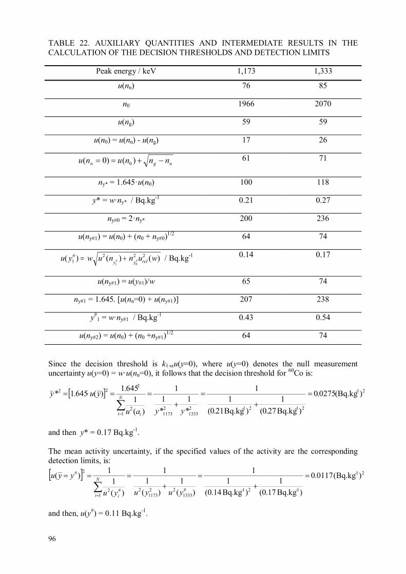
96

TABLE 22. AUXILIARY QUANTITIES AND INTERMEDIATE RESULTS IN THE CALCULATION OF THE DECISION THRESHOLDS AND DETECTION LIMITS

Peak energy / keV 1,173 1,333

u(nn) 76 85

n0 1966 2070

u(ng) 59 59

u(n0) = u(nn) - u(ng) 17 26

ngn nnnunu −+== )()0( 0 61 71

ny* = 1.645·u(n0) 100 118

y* = w·ny* / Bq.kg-1 0.21 0.27

ny#0 = 2·ny* 200 236

u(ny#1) = u(n0) + (n0 + ny#0)1/2 64 74

u y w u n n u wy y rel( ) ( ) ( )#

# #12 2 2

1 0= + / Bq.kg-1 0.14 0.17

u(ny#1) = u(y#1)/w 65 74

ny#1 = 1.645. [u(nn=0) + u(ny#1)] 207 238

y#

1 = w·ny#1 / Bq.kg-1 0.43 0.54

u(ny#2) = u(n0) + (n0 +ny#1)1/2 64 74

Since the decision threshold is k1-αu(y=0), where u(y=0) denotes the null measurement uncertainty u(y=0) = w·u(nn=0), it follows that the decision threshold for 60Co is:

[ ] 21-

21-21-21333

211731

2

222 )Bq.kg(0275.0

)Bq.kg27.0(

1

)Bq.kg21.0(

11

*

1

*

11

)(

1

645.1)(645.1* =

+=

+==⋅=

∑= yyau

yuyN

i i

and then y* = 0.17 Bq.kg-1. The mean activity uncertainty, if the specified values of the activity are the corresponding detection limits, is:

[ ] 21-

1-21-#1333

221173

21

#2

2# )Bq.kg(0117.0

)Bq.kg17.0(

1

)Bq.kg14.0(

11

)(

1

)(

11

)(

11

)( =+

=+

===

∑= yuyuyu

yyuN

i i

and then, u(y#) = 0.11 Bq.kg-1.

97

The detection limit is then: y# = y* + 1.645·u(y#) = 0.17 Bq.kg-1 + 1.645·0.11 Bq.kg-1 = 0.35 Bq.kg-1. 5.4.7. Particular situations

5.4.7.1. Systematic influence on the primary measurement results near the decision threshold

If activities near the decision threshold are measured, the peak location must be performed with high sensitivity in order to locate peaks that have a large uncertainty of the peak area. The main source of uncertainty contributing to the activity calculated from small peaks is the statistical uncertainty. Peaks residing on the continuous background, i.e. when the peaked background is not present, that corresponds to the decision threshold, have a relative

statistical uncertainty of approximately u(0)/y* = 1/1.65. Since )(2)0( gnuu ⋅= , the peak

locating algorithm must locate reliably peaks with a relative uncertainty of about 50%, i.e. with an area that is equal to twice the standard deviation of the continuous background5. Since such a peak interferes with the statistical fluctuations of the continuous background in its vicinity, its area may become substantially smaller or larger than 2·u(ng). In the first case the peak may not be detected and in the second case its area may be overestimated, leading to a systematic overestimation of the activity. It follows that the response of the gamma-ray spectrometer in the vicinity of the decision threshold is not linear. The degree of non-linearity depends on the peak analyzing software and should be assessed in the validation procedure of the software. This non-linearity introduces a systematic influence in the positive direction into the measurement results near the decision threshold on one side and induces type-II errors on the other side.

The correction can be extracted from replicate measurements of the activity of a multi gamma-ray emitter radionuclide radiating at different energies and emitting gamma-rays in a broad range of intensities. From the increase of activities calculated from peaks with a large relative uncertainty over the activities calculated from the peaks with small statistical uncertainties, the correction can be extracted as a function of the relative uncertainty [15]. 5.4.7.2. Sources of measurement bias

In order to report unbiased results all sources of measurement bias must be taken into account. In gamma-ray spectrometry there are two sources of measurement bias, which are independent on the quantity value of the measurand. In the Eq. 159 of the measurement model, they are represented by the quantities X2 and X4. X2 represents the count rate in the peaked background of the spectrometer, measured in the absence of any sample material on the spectrometer. X4 represents contributions of other sources to the count rate in the peaked background i. e. the contribution of interfering peaks and activity of the blank sample.

5 The effective value of the sensitivity parameter that the peak analysis software in the criterion for discriminating statistical fluctuations of the continuous background from small peaks should be set to approximately 2.

98

(a) Background due to the presence of gamma-ray emitters in the spectrometer and its immediate environment

The background of the spectrometer originates in the contamination of the materials of the detector, the gas filling the cavity of the spectrometer shield, the shielding, and the environment of the spectrometer. Disregarding possible contamination of the detector and the shield, the background due to these sources is a property of the spectrometer and is not time-dependent. It is essential to prevent the contamination of the gas filling the shield’s cavity with radon, since this reduces and destabilizes background due to its daughters. To minimize the contamination of the gas filling the detector cavity with radon daughters, flushing of the shield cavity with nitrogen is recommended. To achieve an efficient flushing, the shield’s cavity must be tightly sealed, to prevent the exchange of the gas by the draught. As the gas used for flushing the cavity, nitrogen evaporated from the detector Dewar, may be used. However, when using nitrogen from the Dewar two subjects should be considered. The amount of the nitrogen evaporated may not be sufficient for the flushing. The cavities have ducts for the cold finger, serving as the thermal bridge between the detector cap and the liquid nitrogen in the Dewar, the duct for the cables connecting the detector cap with the pulse-processing electronics and the spaces around the movable side of the shield, which is opened when samples are exchanged. The liquid nitrogen is produced by condensing air, which may contain radon. With the nitrogen also radon is condensed, therefore fresh liquid nitrogen is not radon-free. Since the laboratory has usually no data about the age of the liquid nitrogen delivered, at least some tests on the influence of radon in the liquid nitrogen should be made. The background should be measured when flushing the cavity with fresh nitrogen and liquid nitrogen aged at least ten days. If no influence of the age of the liquid nitrogen on the background of radon daughters is observed for flushing, the nitrogen evaporated in the Dewar may be used. Except for spectrometer shields that are only a few centimeters thick, elimination of radon from the gas filling the cavity stabilizes the background due to radon daughters. In case of thin shields the gamma-rays emitted by radon daughters outside the shield can penetrate it and contribute to the background. In this case the time dependence of this background resembles the time dependence of the concentration of radon in the ambient air. (b) Interferences with gamma-ray emitters present in the sample. In the spectrum, gamma-rays from all radionuclei in the sample, which emit gamma-rays, are registered. If two emitters radiate at energies so close that the corresponding peaks in the spectrum cannot be resolved, the area of the composite peak is the sum of the contribution of both nuclei. To calculate the activity of one of the emitters, the contribution of the other emitter must be subtracted. This contribution presents a source of measurement bias, i.e. a kind of background, which must be corrected for. If one of the interfering emitters radiates at more energies, its activity can be calculated from other lines and the corresponding number of counts subtracted from the composite peak. Then the activity of the other gamma-ray emitter is calculated from the difference.

99

Illustrative example: interference between 235U and 226Ra A major interference in environmental radioactivity measurements is the interference between 235U and 226Ra, radiating at 185.7 keV and 186.2 keV respectively. Since this is the only energy where 226Ra radiates, it is not possible to use the composite peak for the determination of the 235U activity without knowledge of the degree of the secular equilibrium between radon daughters and radium in the sampled material. Because radon may diffuse from the sample, the disequilibrium between radon daughters and 226Ra may be significant. Since the peak at 185.7 keV is the strongest peak belonging to 235U in the spectrum, it is also not convenient to use other peaks for calculating the contribution of 235U to the composite peak in order to determine the activity of 226Ra, because small peaks induce a large uncertainty of its activity. The only possibility remaining is to suppose the natural isotope ratio of the uranium isotopes 235U and 238U and to calculate the 235U activity from the activity of 238U. The activity of 238U is calculated from the activity of its daughter 234Th, radiating at 63.3 keV and 92.6 keV. Since the peak at 92.6 keV interferes with the X-rays of thorium, for the calculation of the 238U activity the peak at 63.3 keV is used. Then, by subtracting the contribution of 235U from the area of the composite peak at 186 keV the activity of 226Ra can be calculated. (c) Contribution of the blank sample During sampling or sample preparation, auxiliary materials may be used that contain measurable activities of gamma-ray emitters. These materials are necessary to preserve the integrity of the sample and are measured simultaneously with the sampled material. If the auxiliary materials contain the same gamma-ray emitters as the sampled material, they induce a peaked background, which contributes to the blank indication. To arrive at unbiased results, the blank indication must be subtracted from the indication [15]. The blank indication may be measured by measuring the peak count rates due to the blank sample. Then the peaked background originates from the spectrometer background and the activity of the blank sample. If the blank indication is used for correcting the indication for the background contribution, the shielding factor is taken into account and must be set to unity in the measurement model. 5.4.7.3. Impact of the width of the region-of-interest

In gamma-ray spectrometry, information on the activities present in the test sample is retrieved from the peaks appearing in the spectrum. Regarding a specified gamma-ray emitter, during a spectrum analysis, two possibilities arise: a gamma-ray emitter is detected in the spectrum or is not detected. When calculating decision thresholds and detection limits, the region-of-interest corresponding to the peak must be used in any of the cases, but the width of the region is different when the gamma-ray emitter is identified or not. When the gamma-ray emitter is identified, the data of the peak analysis are available, therefore the continuous background was already determined and the region-of-interest comprises only the peak region, which is used for calculation of the gross number of counts ng.

100

This number comprises the total number of counts in the peak region regardless if they belong to the net indication, the sources of the measurement bias, the tails of overlapping peaks or the continuous background. It is important to include a great majority of counts, which belong to the net indication into ng. On the other hand, the uncertainty of the net indication increases by increasing the width of the peak region. Therefore this width is a compromise; the ISO 11929:2010 standard recommends the width of 2.5 FWHM for expressive peaks (page 27, Eq. C9). If the gamma-ray emitter is not detected, two possibilities arise: it was not detected, because its peak was deleted since its peak count rate is smaller than the peaked background count rate (the measurement bias) or its peak was not located at all. In any of these cases the data for the calculation of the decision threshold must be retrieved from the channel contents. The easiest way to do it is to use an interactive peak analysis program (e.g. Canberra’s interactive peak search program or equivalent), where the peak and its immediate vicinity can be fitted with a continuous background and a Gaussian function describing the peak shape. In this way the peak data can be restored and the width of the region of interest, being equal to the width of the peak region, which is 2.5 FWHM wide, is used for determining ng. If the software for interactive peak analysis is not available, the peak data for isolated peaks must be retrieved manually from the spectrum. Then, the peak region can be set manually to cover the peak and ng is the total number of counts in the peak region. The region-of-interest comprises besides the peak region also the regions in the immediate vicinity of the peak, from where the continuous background is interpolated in the peak region. If the peak was not located, ng is determined from the peak region, which is 1.2 FWHM wide [4, p. 27 Eq. (C10), 13]. In gamma-ray spectroscopy software packages this method is usually implemented. The user may adjust the width of the peak region and the coverage probability. u(n0) can be determined by the user manually only if the peak region does not overlap with a peak in its vicinity, i. e. in the case when the continuous background can be interpolated into the peak region. When the peak region overlaps with a neighboring peak, the software for interactive peak analysis must be used by inserting manually a peak at the energy where the gamma-ray emitter radiates. It should be noted that in manual analysis, at least in principle, for isolated peaks the uncertainty of the number of counts in the peak region u(n0) can be made as low as needed by extending the energy range, from where the continuous background is interpolated under the peak. However, the uncertainty of the indication as well as the uncertainty of the number of counts in the peak region contribute as follow: u (np) = u (n0) + ng

1/2. Therefore an optimal width of the region of interest exists, which, using a wider region-of-interest, does not decrease the uncertainty of the net indication [11]. If the response of the spectrometer to gamma-rays, i.e. the peak shape, exhibits a strong tail towards low energies, in order to cover a large part of the response of the gamma-rays registered in the peak, a wider peak region may be used. This is often necessary in case of expressive peaks, where its low-energy tail dominates the continuous background. Then the peak region may not be positioned symmetrically around the peak maximum and its width should cover the low-energy tail up to the region where it does not dominate the continuous background any more.

101

6. REPORTING OF RESULTS

6.1 INTRODUCTION The measurement result is a set of values being attributed to the measurand, together with any other relevant information. It follows from this definition that the probability density distribution or probability mass distribution associated with the measurement result must not have a substantial part extending into the region where the value of the result cannot be interpreted consistently with the basic properties of the measurand. Therefore, measurement results of activities, having a significant part of the probability density distribution in the range of negative activities, must be converted to a form that is consistent with the general definition. There are several methods of conversion because the method of conversion is related with the interpretation of the results. Two possibilities are often used for reporting activity measurement results with the probability density distribution that extends into the region of negative activities: conversion to single-sided intervals or conversion to best estimates. Each of these possibilities has its disadvantages. The conversion to single-sided intervals introduces a loss of information that is the larger the coverage probability is and the smaller the limit of quantification is. Also, single sided intervals cannot be used in calculations. The possible conversion back to two-sided intervals is accompanied with an additional loss of information and an introduction of systematic influence if the primary measurement results are not available. The ISO 11929:2010 standard requests conversion of observations to best estimates using the Bayesian posterior. 6.2. METHODS OF CONVERSION

Conversion to single-sided intervals, i.e. reporting in a form “< f [y, u(y)]” Here f represents a function of the measurement result, expressing the upper boundary of the interval of activity values covering a predetermined part of the probability density distribution defined by the primary measurement result. It is recommended that the probability density interval comprises 95% of the probability density distribution. In this case f [y, u(y)] = y + 1.645·u(y). The range of the relative uncertainties, where the conversion is performed, is the limit of quantification and reflects the policies of the laboratory, the customer and the regulatory body. At relative uncertainties exceeding the limit of quantification, the primary measurement result is deemed unquantifiable and is reported as an upper limit. Conversion to best estimates using the Bayesian posterior When calculating best estimates with the Bayesian posterior [4], the uncertainty of the best estimate is always smaller than the value of the best estimate, therefore the interval defined by the best estimate value and its uncertainty )ˆ(ˆ yuy ± does never extend into the region of negative activities. However, this interval does not have a coverage probability independent on the relative uncertainty u y y( $) / $.

102

The conversion of primary measurement results to best estimates introduces a systematic influence in the positive direction into the reported results, which is the larger the larger the relative uncertainty of the primary measurement result is. Also, these results may lead to unacceptable conclusions when used in subsequent calculations, such as calculation of means, seasonal variations and trends. To illustrate the systematic influence introduced by the conversion of primary measurement results to best estimates, measurements results for a blank sample are presented. It is clear that, for unbiased measurements, their mean must assume a zero value within its uncertainty. When the primary measurement results assume values of y ± u(y) and –y ± u(y) the mean value is 0 ± 2-1/2

u(y), but the mean of best estimates is always greater than zero. In Table 23 the weighted mean of the two estimates, calculated with weights being inversely proportional to the variance of the best estimates, is given for various values of the relative uncertainty u(y)/y. In the table also the a-priori and a-posteriori uncertainties are given, calculated from the uncertainties of the best estimates and the dispersion of the best estimate values. TABLE 23. THE MEAN VALUES OF TWO BEST ESTIMATES CORRESPONDING TO TWO PRIMARY MEASUREMENT RESULTS y ± u(y) AND –y ± u(y) HAVING A MEAN VALUE OF ZERO AT DIFFERENT RELATIVE UNCERTAINTIES u(y)/y

u(y)/y

%

Observed values

Best estimates Weighted

mean

A-priori

uncertainty

A-posteriory

uncertainty

∞ 0 (0.80 ± 0.60)·u(y) (0.80 ± 0.60)·u(y) 0.80·u(y) 0.42·u(y) 0

1000 ± 0.10·u(y) (0.84 ± 0.62)·u(y) (0.76 ± 0.58)·u(y) 0.80·u(y) 0.42·u(y) 0.02·u(y)

150 ± 0.67·u(y) (1.10 ± 0.73)·u(y) (0.60 ± 0.49)·u(y) 0.76·u(y) 0.41·u(y) 0.12·u(y)

100 ± u(y) (1.29 ± 0.79)·u(y) (0.53 ± 0.45)·u(y) 0.72·u(y) 0.39·u(y) 0.16·u(y)

60 ± 1.67·u(y) (1.77 ± 0.90)·u(y) (0.41 ± 0.37)·u(y) 0.61·u(y) 0.34·u(y) 0.24·u(y)

30 ± 3.33·u(y) (3.33 ± 1.00)·u(y) (0.26 ± 0.25)·u(y) 0.44·u(y) 0.24·u(y) 0.36·u(y)

25 ± 4.00·u(y) (4.00 ± 1.00)·u(y) (0.22 ± 0.22)·u(y) 0.40·u(y) 0.21·u(y) 0.40·u(y)

It follows from the table that the a-priori uncertainty is always smaller than the mean, therefore the true value (zero) lies always outside the confidence interval defined with the mean and its a-priori uncertainty. On the other hand, the a-posteriori uncertainty approaches the mean at low relative uncertainties of the primary measurement result. It can be concluded that the mean of the best estimates calculated with the Bayesian posterior does not agree with the primary measurement results and that the procedure of averaging best estimates of observations near the natural limit is not acceptable.

103

It should be mentioned that the standard uncertainty intervals of the best estimates do not correspond to the same coverage probability [20], because the shape of the distribution of the true values depends on the relative uncertainty. If the observed value is much larger than its uncertainty the distribution resembles the normal distribution, but at observed values smaller than zero it resembles just a tail of it. Therefore also the standard uncertainty intervals of the mean do not correspond to a coverage probability that is independent on the measurement uncertainty. Nevertheless, it can be observed that the true value (zero) lies always outside the uncertainty intervals of the best estimates and also outside the intervals given by the a-priori and a-posteriory uncertainties of the mean. It can be concluded therefore that the results of calculations with best estimates and their uncertainties do not represent quantities that are consistent with the primary measurement results. Therefore the Analytical Methods Committee recommends that the method for reporting should be decided in the context in which the measurements were performed [21]. If the measurements were performed for the purpose of comparison with a legal limit or for assigning a property value the best estimates should be reported. If the measurement results are intended for subsequent calculations or statistical analyses primary measurement results should be reported. In Table 24 are presented methods to report upper limits based on observations and quantities that are recorded according to the ISO 11929:2010 standard. For reporting single-sided intervals, the coverage probability is 95%. The limit of quantification is set to 30%. The coverage interval is calculated for the coverage probability of 95% for the probability density distribution of true values. The standard does not require recording the limits of the coverage interval and the best estimate, if the observed value is smaller than the decision threshold. TABLE 24. SINGLE-SIDED INTERVALS, DECISION THRESHOLDS, DETECTION LIMITS, LIMITS OF THE COVERAGE INTERVALS AND BEST ESTIMATES AS FUNCTIONS OF THE OBSERVED VALUE AND ITS UNCERTAINTY

Observation Single-sided

intervals

Decision threshold

y*

Detection limit

y#

Lower limit

y◄

Upper limit

y►

Best estimate $ ( $)y u y±

0 ± 1.00 < 1.65 1.65 3.95

0.30 ± 1.03 < 2.00 1.65 3.95

1.00 ± 1.10 < 2.82 1.65 3.95

1.65 ± 1.17 < 3.84 1.65 3.95 0.18 3.99 1.84 ± 1.01

3.33 ±1.33 < 5.52 1.65 3.95 0.86 5.94 3.35 ± 1.30

5.00 ± 1.50 5.00 ± 1.50 1.65 3.95 2.06 7.94 5.00 ± 1.50

104

6.3. COMMENTS ON THE METHODS OF CONVERSION Regarding the measurement results, the ISO 17025:2005 standard requests that the results must be reported accurately, clearly, objectively and unambiguously. Also, they must be fit for the purpose. Besides that, the ISO 17025:2005 standard requests that the interpretation of the measurement results must be clearly marked in the report. The conversion of primary measurement results to best estimates is a kind of interpretation, since the conversion using the Bayesian theorem with the prior function which is zero at negative observed quantity values and unity elsewhere is not the only method to perform the conversion. It follows therefore from the requirement of the ISO 11929:2010 standard that the primary measurement results should be reported simultaneously with the best estimates. Two questions arise from this requirement:

How to report primary measurement results with a substantial part of the probability density distribution beyond the limit of quantity values, which are physically admissible, without loss of information?

How to report the results clearly, accurately and unambiguously? Reporting both, primary measurement results and best estimates, conflicts with the request that the results must be reported unambiguously. Although the basis, on which the conversion of primary measurement results to best estimates is made, is described in the test report the user may be uncertain which kind of the results is more reliable or more accurate. To resolve the dilemma about reporting primary measurement results or best estimates calculated according to the Bayesian approach and to fulfill at least the requirement that the results should be fit for the purpose, it is proposed to follow the advice of the Royal Society of Chemistry [21] that what to report is to be decided by the reporting organization on the basis of the knowledge on the intended use of the results. When reporting primary measurement results, the conversion to single-sided intervals must be made when a large fraction of the probability density function extends in the range of negative activities. When reporting best estimates, no conversion to single-sided intervals is necessary. If, for the intended use of the results reported, a comparison with other values, e.g. the comparison with guideline values or determination of property values for the purpose of certification, is requested, then best estimates are reported. On the other hand, if the results are intended to be used in further analyses, e.g. in dose assessments or long-term environmental studies, primary measurement results are reported. The limit of quantification, which expresses the largest relative uncertainty to be reported, should be established according to the need for data. The larger the need is, the smaller the loss of information should be and the larger the limit of quantification is.

105

Example: When assessing the ingestion dose from gamma-ray spectrometric results, it is important to assess the massic activity of 210Pb, which is a member of the uranium decay chain and is generally present in the natural and living environment. From naturally occurring gamma-ray emitters it has the largest dose conversion factor for ingestion, therefore it is essential to use as much as possible information for determining its contribution to the dose. It emits gamma-rays at the energy of 46.5 keV, therefore its concentration in many kinds of foodstuff is around or below its decision threshold. To assess the dose as realistically as possible, any value of the net indication, which can be attributed to 210Pb should be taken into account, together with its uncertainty, from where the uncertainty of the assessed dose follows. Since the dose due to 210Pb is summed with doses of other radionuclides, the activity of 210Pb is used as an input to a subsequent calculation and the primary measurement result should be reported. 6.4. RELATIONS AMONG ISO 11929:2010, ISO 18589:2014 AND ISO 17025:2005

STANDARDS REGARDING REPORTING OF MEASUREMENT RESULTS The ISO 11929:2010 standard does not prescribe any content of test reports on measurement results, it prescribes only which data are to be retained in order to maintain traceability. According to this standard, the content of test reports is subject to agreement between the reporting body and its client. The observed value is compared to the decision threshold and on the basis of this comparison it is possible to conclude on the presence (or the probability of presence) of the analyte in the sample. According to the ISO 11929:2010 standard, an observed value smaller than the decision threshold indicates that the analyte is not detected, although it cannot be concluded that it is absent from the sample, because then the corresponding indication is not attributed to the analyte. The detection limit, on the other hand, offers the information about the analytical procedure which was used for the measurement. From the comparison of the detection limit with a guideline value (e.g. a legal limit), it can be concluded on the suitability of the measurement procedure for determining the value of the measurand (property value) for the purpose of comparing it with the guideline value. Guideline values pose restrictions on property values, therefore a detection limit that exceeds a guideline value indicates that the measurement procedure is not appropriate to determine a property value for the purpose of comparing it with the guideline value. The ISO 18589-3:2014 standard [22] on the other hand, prescribes the contents of the test report. Depending on the customer’s request, the measurement result: — should be presented as < y* when the measured value is below the decision threshold, or

— it can be expressed as < y# when the measured value is below the detection limit. If the detection limit exceeds the corresponding guideline value, it shall be documented that the method is not suitable for the measurement purpose. When the measurement result is presented in the form < y# the detection limit assumes the function of a limit of quantification, which corresponds to the relative uncertainty u(y#)/y# = (1 – y*/y#)/k1-β, which equals approximately to a relative uncertainty of 30% when k1-β = 1.645 and y# = 2·y*.

106

It should be stressed that peak-analyzing programs introduce censoring of peaks, when they are based on a peak locating algorithm. Censoring depends on the value of the sensitivity parameter S, which defines the criterion for differentiating fluctuations of the continuous background from peaks. Peaks with an area np < s·ng

1/2, where s denotes the value of the sensitivity parameter, are not expected to be located. Therefore for peaks residing on a flat

continuous background, the indication gg nns ⋅+± )1( κ , where κ denotes the ratio of the

number of channels in the peak region and the number of channels used for determining the background under the peak, may not be reported. It follows that indications with a relative

uncertainty s/)1( κ+ may be censored. Since the number of counts corresponding to the

decision threshold is gy nkn ⋅+⋅= − )1(1* κα , an indication corresponding to the decision

threshold is reported only if gg nsnk ⋅>⋅+⋅− )1(1 κα , from where κα +⋅< − 11ks follows.

Assuming k1-α = 1.645 and κ = 1, the maximal value for reporting of results near the decision threshold is s = 2.33. At values of the sensitivity parameter greater than 2.33 the observations with the value corresponding to the decision threshold are censored with a large probability [18]. The interpretation that, for measurement outcomes without the identification of the measurand, its true value lies below the decision threshold is misleading if the peak analysis procedure was performed with a value of the sensitivity parameter in excess of 2.33. Such an interpretation is defensible only if the indications with a value corresponding to the decision threshold are expected to be reported with a large probability. In computerized gamma-ray spectrometric analyses the actual limit of detection, or better the limit of reporting, is defined by the value of the sensitivity parameter and not only by the physical characteristics of the spectrometer defining the null measurement uncertainty. The statement that an observed value cannot be attributed to the measurand if its value is smaller than the decision threshold is an interpretation. Therefore it should be clearly marked as such in the test report. Also, this interpretation [4, p. 15] may conflict with the requirement of the ISO 17025:2005 standard on the objectivity, since objectivity means proceeding from the object of knowledge or taught as distinct from the perceiving or thinking subject (The Concise English Dictionary). It should be observed that, according to this definition of objectivity, objectively interpreting means interpreting according to the larger probability. In interpreting or expressing opinions the reporting body may, in contrast to reporting results which shall be reported objectively, explain its view regarding the results. Therefore the ISO 17025:2005 standard requires that interpretations shall be clearly marked [1, Clause 5.10.5]. When measurement results below the decision threshold are quoted as ‘< y*’, the interpretation that this result is not attributed to the measurand should be marked as an interpretation.

107

6.5. SUGGESTED APPROACHES FOR REPORTING On completion of the analysis, the results should be calculated and the supporting data, including the appropriate quality control checks, should be provided. If no gross errors are revealed and all of the relevant quality control measurements are within control, the results – �, ��,

\O�\�, �∗, �#, �� and �� – should be calculated6 and are then ready for reporting.

The final step in this process is to round the data appropriately; it is imperative that this is the last step of the calculation process, since rounding earlier in data processing risks losing accuracy. The result should be rounded to the required number of significant figures and the expanded uncertainty rounded up to the same resolution. For example:

1.234567 ± 0.00123 may be rounded to 1.235 ± 0.002 1.2345 ± 0.0123 may be rounded to 1.235 ± 0.013

1.234 ± 0.123 may be rounded to 1.23 ± 0.13 1.234 ± 0.543 may be rounded to 1.2 ± 0.6

With the data processing and rounding completed the data may be reported as follows. 6.5.1. Measurements in the region ^ < ^∗ (below the decision threshold)

If � < �∗, then the effect is not observed. As set out in the ISO 11929:2010 standard, this relates to count data, and not the final result; it is therefore possible to say that the detected count rate of the source is < �∗7 and that no activity that can be distinguished from the background signal has been detected. It is, of course, possible that the radionuclide being sought is indeed present, but at levels below the detection capability of the technique employed; it may be possible to detect a signal from this radionuclide in such cases with other measurement and analysis technologies. In this case, it is possible to say that the effect is ‘not detected’ and therefore there is < �∗in the measurement source. This report can be qualified with a statement such as: ’This is the detection limit for

mA in this analysis;

mA has not been detected in this analysis.’

This value may vary between samples where variations of chemical yield or efficiency may be observed and may need further explanation to the customer.

6.5.2. Excessive values for ^#

Examination of the equation to calculate �# implies that large values of �# may occur. This will happen when there is a condition where the value of �# becomes infinite:

0 → �Oijk�]� ; �# → ∞ (218)

6 It may not be necessary to calculate all of these values.

7 Or counts emitted in a given time period, depending on the case.

108

The conditions under which this may happen are when the pooled relative uncertainties on the terms making up � are large. Using the general equation set out in Section 4, the causes may be narrowed down as follows:

• The parameters related to nuclear decay data (L and M) will generally result in relative uncertainties far below 5%.

This is not the case for mass measurements (I), chemical recovery (J) and counting efficiency (K), where large uncertainties may arise.

• Mass measurements made close to the performance limits of the balance. A review of such data should make this clear, and the measurement should be repeated.

• Poor chemical yields can be rejected by monitoring chemical yield results for the analysis with a suitable control chart. Very low chemical yields will manifest themselves as action limit violations, triggering a repeat of the analysis.

• Poor counting efficiency can similarly be rejected by monitoring counting efficiency results for the analysis with a suitable control chart. Again, very low counting efficiency will manifest themselves as action limit violations, triggering a repeat of the analysis.

• Gross errors in the course of an analysis, such as spillage, should be noted and should trigger an investigation and repeat of the measurement.

6.5.3. Measurements in the region y* < y < y

# (between decision threshold and detection

limit)

If y* < y < y#, then the effect is observed, but not quantifiable.

In this case, it is possible to say that the effect is ‘detected’ and therefore there is < �#in the measurement source. This report can be qualified with a statement such as:

‘It is possible that mA has been detected, but it is not quantifiable in this analysis with

detection limit �#.’ 6.5.4. Measurements in the region ^# < ^ < �. ��^� (slightly above the detection limit)

If �# < � < 4. ��, it is possible to make a best estimate �� of the result as stated in Section 4.6, although the result is transformed as described in that section. In this case, the uncertainty of ��, ��, is smaller than the measurand uncertainty, �� and in the region 1.8 < \O�\� < 4 then: Q�� + ��R < Q� + ��R (219)

This condition may lead to the small possibility that a measurement result may genuinely fall outside of the confidence limits set by��±��.In the region

\O�\� < 4, then this problem

disappears. The result may be reported as: �� ± 0. ��

109

This report may be qualified with a statement such as: ’m

A has been identified and quantified in this analysis, although the result is close to the

detection limit, �#, which is reflected in the relatively large uncertainty.’

6.5.5. Measurements in the region ^ > �. ��^� (unambiguously above the detection

limit)

Results in this region are unambiguous and should be reported without any additional qualification as: � ± 0. �� 6.5.6. Toolkit for reporting

Summarising the foregoing, these data, calculated in Section 4, are needed for reporting and should always be calculated. The data used for reporting are given in Table 25. TABLE 25. DATA USED FOR REPORTING

Value Comments 0 Coverage factor for the measurement. �∗ Decision threshold for the measurement. If converted to an activity or massic activity, this may vary within a batch of analyses. �# Detection limit for the measurement. If converted to an activity or massic activity, this may vary within a batch of analyses.

�� Best estimate of �, when \

O�\� < 4.

�� Best estimate of ��, when \

O�\� < 4.

� Calculated value without modification. �� Calculated uncertainty without modification.

With this information available, the result can be reported, using the suggested strategy, with the provision that such an approach is consistent with the laboratory’s quality system. The proposed reporting of results is summarized in Table 26.

110

TABLE 26. REPORTING OF RESULTS

Condition Report Comments

� < �∗ < �∗

The effect is not detected. Qualify this information with: ’This is the detection limit for

mA in this analysis;

mA has

not been detected in this analysis.’

�∗ < � < �# Detected,

< �#

The effect is detected, but not quantifiable. Qualify this information with: It is possible that

mA has been detected, but is not

quantifiable in this analysis with detection limit �#.’

�# < �< 4. ��

�� ± 0. ��

A best estimate of the result may be reported. This information may be qualified with: ‘m

A has been identified and quantified in this analysis,

although the result is close to the detection limit, �#, which

is reflected in the relatively large uncertainty.’

4. �� < � y ± 0. ��

The result may be unambiguously reported and no additional qualification is needed. It may be instructive for the user if this statement is made: ‘m

A has been unambiguously identified and quantified in

this analysis, where the detection limit for this analysis is �#’

7. CONCLUSIONS

This publication deals with the many aspects emerging in the implementation of the ISO 11929:2010 standard for radioactivity measurements. The ISO 11929:2010 standard has a far reaching range of applicability since it practically involves all methods of radioactivity measurements and relates to the reporting of the measurement results. More specifically it deals with the judgment whether a signal has been detected or not by defining the decision threshold or the detection limit, the level at which quantitative measurements can be made. All ISO standards currently referring to the ISO 11929:2010 standard have been listed in this report. For many decades, laboratories all over the world have been using the Currie formalism to express the quantities decision thresholds and detection limits for specific radioactivity measurement methods. Working expressions derived from the Currie formalisms have been included in many spreadsheet applications for the treatment of nuclear measurement data and have also been implemented in nuclear counting and analysis software. The ISO 11929:2010 standard uses a more universal formalism to derive the characteristic limits compared to the Currie formalism [9] and also copes with some limitations of this approach. The ISO 11929:2010 standard relies on the basic expressions of uncertainty for the quantity to be measured (activity or activity per volume, mass) and hence relies on the basic theory of uncertainty estimation as it has been presented in the guide to the expression of uncertainty in measurement (GUM) [8]. Basic statistical concepts applicable in uncertainty estimation are also added in an annex to this report.

111

Therefore the implementation of the concept of decision thresholds and detection limits in testing laboratories is a substantial step forward in the direction of presenting the quality of the measurements in a standardized, systematic and easily surveyable way. This publication focuses on the commonly applied radioactivity measurement techniques, e.g. gross alpha and beta counting, liquid scintillation counting, alpha spectrometry and gamma-ray spectrometry, to develop equations to be used for the determination of the characteristic limits. Detailed formulae are worked out for the uncertainty of the measured radioactivity using specific models and from that the quantities decision thresholds and detection limits are derived. For each of these techniques, the commonly used methods in the laboratory are considered, e.g. laboratory analysis may be based on commercial software or data may be obtained from spreadsheet evaluations. In both cases this publication gives a methodology allowing the reader to compute the characteristic limits in its laboratory. Each of the counting options considered also are illustrated with one or more examples, leading the reader stepwise through the calculations. Where appropriate, this publication also compares the results obtained following the ISO 11929:2010 standard with those that are obtained using the Currie approach [9]. It is shown that in many occasions similar results are obtained by both methods. However there are also situations where there is an important difference between both methods. The main deviation between the Currie formalism and the ISO 11929:2010 standard is in the computation of the detection limit for activity (Minimum Detectable Activity (MDA) in Currie approach). The ISO 11929:2010 standard correctly accounts for all the uncertainty components while the Currie approach assumes the conversion factor to go from counts to activity to be a known constant. Best estimate and confidence interval are two other concepts introduced by the ISO 11929:2010 standard. These quantities are based on a reasoning following Bayesian theory that uses the prior knowledge that the physical quantity radioactivity has a non-negative value, although the result of a measurement can be negative. The best estimate and confidence interval are a transformation of the original data to produce positive results while keeping the concept of confidence for the measurand. Negative activity values may appear when the primary measurement result is of the order of the associated measurement uncertainty. When the activity value is much larger than its uncertainty then the best estimate and confidence interval converge to the primary measurement result and its standard uncertainty. This publication details how to compute the best estimate and confidence interval and explains how to use spreadsheet functions to compute these quantities. Since the characteristics limits together with the best estimate and confidence interval are the main components in reporting, all the different reporting conditions that depend on the measurement value have been considered here and have been clearly listed. In appendix also alternative approaches for reporting are given. A particular case of uncertainty estimation is encountered in measurements with only a few counts. A correct treatment of these situations requires modified formulae that are also considered in this publication and that have been elaborated in more detail in an appendix to this publication. This publication shows that characteristic limits are not unique values that only depend on a measurement apparatus, but also depend on the computational procedures, models used to compute these quantities and many other conditions. When reporting characteristic limits it is important to provide to the user of the results with all details that have led to these values.

112

For gamma-ray spectrometric measurements the post-treatment of the peak analysis results renders the calculation of decision thresholds and detection limits easy and versatile. This method simplifies the calculations of the decision thresholds and detection limits considerably, because it exploits the results of the peak analysis regarding the continuous background and the influence of the overlapping peaks. However, the Bayesian approach of the ISO 11929:2010 standard requires a firm assessment of the uncertainties. The conversion of observations to best estimates introduces a dependence of the best estimate value on the uncertainty of the observed value. To prevent a systematic influence originating in erroneously assessed uncertainty of the primary measurement result on the best estimate value, the uncertainties should be assessed realistically, taking into account all known sources. This is especially important for measurements where measurement results near the decision threshold are abundant. Here the sources of uncertainty affecting the uncertainty of the blank indication have an influence that is typically larger than the influence of uncertainties contributing to the conversion factor. Therefore knowing the sources of measurement bias is essential for a reliable estimation of the blank indication and its uncertainty. Reporting of results should be performed objectively, clearly and unambiguously. The interpretations should be separated and clearly marked. If a measurement result with the value smaller than the decision threshold is quoted as < y* the comment that it was not observed or not detected should be marked as an interpretation.

113

APPENDIX I

UNCERTAINTY ESTIMATION

I.1. BASIC STATISTICAL CONCEPTS RELATED TO ASSESSMENT OF UNCERTAINTIES Most commonly, the uncertainty of a variable X is given as the standard deviation σ, which is the positive square root of variance:

N�� = TVar�X� (220)

The variance can be defined with the help of expected value E[X]:

Var�� = Ep�X-E[X]�5q (221)

For random variables following normal distribution, the probability of detecting an event within certain interval is directly set by the expected value and standard deviation of the probability distribution, as shown in Table 27. TABLE 27. CONFIDENCE INTERVALS FOR NORMAL DISTRIBUTION

Lower limit, �⊲ Upper limit, �⊳ Probability

�[X] �[X]+σ(X) 0.34 �[X]-σ(X) �[X] 0.34 �[X]-σ(X) �[X]+σ(X) 0.68 �[X]-σ(X) ∞ 0.84 .∞ �[X]+σ(X) 0.84 �[X] �[X]+2σ(X) 0.48

�[X]-2σ(X) �[X] 0.48 �[X]-2σ(X) �[X]+2σ(X) 0.95 �[X]-2σ(X) ∞ 0.98 .∞ �[X]+2σ(X) 0.98

I.1.1. Uncorrelated variables

Let us consider a variable Y expressed as a function of two random variables (��, �5) and two constants (>�, >5). The random variables are first assumed to be uncorrelated. In this case, the following equations apply precisely:

if � = >�. �� + >5. �5, then N�� = T>�5. N5�� + >55. N5��5� (222)

and if � = >�. �� . >5. �5, then N�� = T>�5. N5�� + >55. N5��5�

(223)

114

In a case where Y is an arbitrary function of �� and �5, some approximations are typically needed. A common practice is to linearize Y with respect to �� and �5. Then, the equations above are applied for the linearized function:

� = ¼��, �5) N(�� [ UV �¿� ¡W5 . N5�� + V �¿

� lW5 . N5��5� (224)

This approximation is often adequate for uncertainty estimation. It is reasonably accurate as long as the function f behaves somewhat linearly when �� = [E[��] . 2 · N��, E[��] + 2 ·N��] and �5 = [E[�5] . 2 · N��5�, E[�5] + 2 · N(�5)]. However, it should be noted that Y

does not generally strictly follow the normal distribution and the standard deviation of Y may not even be defined. The uncertainty of the product and ratio of random variables can be assessed by using the approximate approach presented in Eq. 222:

� = ��. �5 then N�� [ T�55. N5�� + ��5. N5��5� (225)

� = ��/�5 then N�� [ UV �

lW5 . N5�� + V ¡ llW5 . N5��5� (226)

The equations can also be generalised for more than two input parameters X. For example, Equation 224 for n input parameters is:

� = ¼��1 , �2 …�')N�� = U∑ V "¼"� W2' =1 . N2(� )

(227)

I.1.2. Correlated variables

The values of correlated variables depend on each other. The linear dependence between two random variables (��, �5) can be expressed with Pearson’s correlation coefficient [23]:

#��, �5) = �p:�� . # ¡;. :�5 . # l;qN��. N��5� (228)

The values of #��, �5) range from -1 to +1. Table 28 presents interpretations for the values.

TABLE 28. INTERPRETATIONS OF THE VALUES OF CORRELATION COEFFICIENT

Correlation coefficient #��, �5) Interpretation Example

-1 Perfect negative correlation �� + �5 = $ [-1,0[ Negative correlation

0 No correlation ]0,1] Positive correlation +1 Perfect positive correlation �� . �5 = $

115

Let us again consider a variable Y expressed as a function of two random variables (��, �5) and two constants (>�, >5). If the values of �� and �5 are significantly correlated, Eqs 222-227 derived for uncorrelated variables are not valid. Instead, equations presented in Table 29 should be used, which also take into account the correlation. If the correlation is neglected, the uncertainty of the variable Y may be either over- or underestimated. TABLE 29. STANDARD DEVIATIONS FOR Y DEFINED AS A FUNCTION OF CORRELATED RANDOM VARIABLES X1 AND X2

Function � Standard deviation N�� >�. �� + >5. �.5 T>�5. N5�� + >55. N5��5� + 2>�. >5. N��. N��5�. #��5, �� (1) >�. �� . >5. �5 T>�5. N5�� + >55. N5��5� . 2. >�. >5. N��. N��5�. #��5, ��(2) ¼��, �5) ≈UV �¿

� ¡W5 . N5(�� + V �¿

� lW5 . N5��5� + 2. �¿� ¡

�¿� l . N��. N��5�. #��5, ��

(3) ��.�5 [ T�55. N5�� + ��5. N5��5� + 2. �5. ��. N��. N��5�#. ��5, ��(4) ��/�5 [ UV � lW5 . N5�� + V ¡

llW5 . N5��5� . 2. ¡ lÚ . N��. N��5�. #��5, ��

(5) Unfortunately, the correlation coefficients are not always available. However, it is easy to deduce whether the correlation is insignificant, positive or negative. If the correlation is insignificant, the correlation coefficient can be set to zero. If the correlation is significant and positive, either the value 0 or 1 should be used for the coefficient. The selected value should maximize the uncertainty of Y. If the correlation is significant and negative, either 0 or -1 should be used. Again, the value maximizing the uncertainty should be selected. I.2. UNCERTAINTY COMPONENTS IN RADIOACTIVITY MEASUREMENT Section 4 defined the general equation linking an activity or massic activity to observed counts as: >� = �¬AD.F.G.E.H (229)

In this case, the multiplier � (as denoted in the ISO 11929:2010 standard) is given by: � = �AD.F.G.E.H (230)

Additional terms may be included for specific measurements, and these are detailed in subsequent sections. Common terms are defined in Table 30.

116

TABLE 30. COMMON TERMS FOR UNCERTAINTY COMPONENTS IN RADIOACTIVITY MEASUREMENTS

Symbol Quantity Units Comments =� Massic activity Bq.kg-1 Determined as above ��=�� Massic activity

uncertainty Bq.kg-1

Determined by combination of contributing uncertainties '% Gross sample

count9 Direct observation

�:'%; Gross sample

count uncertainty Derived in Section 4

(I Sample count

time s

Direct observation (may be expressed in minutes or other time units)

)% Gross sample count rate

s-1

May be directly observed, depending on instrument, but can also be derived from gross sample counts and sample count time (see text below).

��)%� Gross sample

count rate uncertainty

s-1 Derived in Section 4

'& Background count Direct observation ��'&� Background count

uncertainty Derived in Section 4

(& Sample count

time s

Direct observation (may be expressed in minutes or other time units)

)& Background count

rate s-1

May be directly observed, depending on instrument, but can also be derived from gross sample counts and sample count time (see text below).

��)&� Gross sample

count rate uncertainty

s-1

Derived in Section 4 )$ Net sample count

rate s-1

��)$� Net sample count rate uncertainty

s-1

I Mass of sample kg Direct observation, although may be recorded as grams (g) or milligrams (mg)

��I� Mass of sample

uncertainty kg Taken from current certificate

K Counting

efficiency of the detector

s-1.Bq-1

Varies, depending on the application and is

dealt with individually ��K�

Uncertainty of the counting

efficiency of the detector

s-1.Bq-1

L Intensity Available from nuclear data tables

9 Although counts are recorded, they are dimensionless and are not given units.

117

TABLE 30. COMMON TERMS FOR UNCERTAINTY COMPONENTS IN RADIOACTIVITY MEASUREMENTS (cont.)

Symbol Quantity Units Comments ��L� Intensity

uncertainty

J Chemical yield (or recovery)

Varies, depending on the application and is

dealt with individually ��J� Uncertainty of the

chemical yield M Radioactive decay

Derived in Section 4 ��M� Radioactive decay

uncertainty

(¸ Sample decay

time s

Set by user (may be expressed in minutes or other time units) ��(¸�

Sample decay time uncertainty

s Set by user (may be expressed in minutes or other time units), and usually insignificant ��/5 Radionuclide

half-life s

Available from data tables (may be expressed in other time units) �:��/5;

Radionuclide half-life

uncertainty s

I.2.1. Counting uncertainty

Radioactive decay is a statistical phenomenon. In radiation measurements, the number of detected counts n follows the Poisson distribution. For Poisson distribution, the standard deviation is directly set by the expected value �[�]10. Therefore, if the expected value of the number of detected counts is known, the standard deviation of the detected number of counts is simply:

N�'� = T�['] (231)

The approach selected in the ISO 11929 standard is to estimate the expected value with the detected number of counts and its uncertainty with Eq. 231:

�['] [ ' and ��[']� [ √' (232) This approximation can typically be considered to be valid when ' > 100 (see further discussions in Appendix IV). The approximation is also used in this document, unless stated otherwise. If the observation is recorded as a count rate ) then, it can be expressed as:

) = $Y (233)

10

The reader is referred to any suitable textbook on radioactivity measurement or statistics for a full explanation.

118

and so:

��)� = O�$�Y = √$Y = U $Yl (234)

Thus, for sample measurement, the following expressions can be written for the background count rate. First, the gross sample count rate is:

)% = $°YD (235)

with: �:)%; = U�°YD = T$°YD (236)

Next, the background count rate is: )& = $gYg (237)

with: ��)&� = U�gYg = T$gYg (238)

It may be useful to calculate the net sample count rate:

)$ = )% . )& = $°YD . $gYg (239)

with:

��)$� = U�5:)%; + �5�)&� = U�°YD + �gYg = U$°YDl + $gYgl (240)

I.2.2. Mass uncertainty

Uncertainty on mass is usually derived from the certificate of calibration for the balance used. Additional uncertainty may be incurred from buoyancy correction and from the resolution of the balance display. These are very small and are unlikely to have any significant impact on the overall uncertainty budget and are therefore ignored. The relative mass uncertainty is:

��I� � O�AD�AD

(241)

I.2.3. Intensity uncertainty

All modes of decay and the associated emission of particles and electromagnetic radiation will take place with a certain probability. For most (but not all) particle emissions, the intensity is taken as 1 – a notable exception is the decay of 40K, which exhibits a β intensity of 0.8925 (± 0.0017). This is not the case for X- and gamma-ray emissions and suitable data tables should be consulted for up to date values.

119

The relative intensity uncertainty is: ��L� = O�G�G (242)

In the case of 40K, stated above, ��L� [ 0.0019 In the case of alpha- and beta-particle emissions, the uncertainty could be assumed to be zero if the measurement region of interest embraces the entire emission of the radionuclide in question. This may be illustrated as follows for a 209Po alpha-particle emission using the decay data given in the Decay Data Evaluation Project (DDEP) [24]: Decay scheme: Po-209 disintegrates by alpha emissions (99.546 (7) % to excited levels and

to the ground state level in Pb-205 and by electron capture (0.454 (7) %) to

the excited level of 896.3 keV in Bi-209.

Alpha transitions: 4716.4 (14) keV 0.548 (7) %

4976.9 (14) keV 79.2 (32) %

4979.2 (14) keV 19.8 (32) %

If it is assumed that the region of interest covers the energy zone 4700-5000 keV, then the value for Pα could be taken as 0.99546 (± 0.00007), i.e. a relative uncertainty of ± 0.0071%. However, the summation ∑�L Ö%�& + L ÖÙ%& + L ÖÙ%Ù� gives 0.99548 (± 0.04526), i.e. a relative uncertainty of ± 4.546%. In this case the first (and lower) uncertainty should be used. It is therefore important to evaluate the decay data used. I.2.4. Decay uncertainty

The decay correction used for calculating an activity at some given point is given by:

M = w§ÇÈ g.É.¯'Ê¡/l ¨ (243)

Using the equation given in A2.2.1, where ( = ). w�.P:±O�P�;, then ��(� = (. =. ��and ��(� = =. �� and ) = 1, = = ln0.5 and � = Y'� , then:

� x Y'�¡/lz = Y'�¡/l . ¢VO�Y'�Y' W5 + xO:�¡/l;�¡/l z5 (244)

Usually, O�Y'�Y' ≪ O:�¡/l;�¡/l� , but this is not always the case, collection and count times should be

evaluated, so:

��(¸� = UYDl�5 + Y�l

�5 (245)

120

The sampling period, (�, and the counting time, (I, have a rectangular distribution hence they are divided by √12 to convert these to a normal distribution; events have an equal probability of occuring at any time during these periods, so:

��(¸� = U:YDlhY�l;�5.Y'l (246)

and so:

� x Y'�¡/lz = Y'�¡/l . ¢:YDlhY�l;�5.Y'l + xO:�¡/l;�¡/l z5 (247)

thus:

��M� = �� &.+.Y'�¡/l . ¢:YDlhY�l;�5.Y'l + xO:�¡/l;�¡/l z5� . w§ÇÈ g.É.¯'Ê¡/l ¨ (248)

and:

��M� = �� &.+.Y'�¡/l . ¢:YDlhY�l;�5.Y'l + xO:�¡/l;�¡/l z5 (249)

I.2.5. Overall uncertainty

The general equation linking a massic activity to observed counts is:

=� = �¬AD.F.G.E.H (250)

and the uncertainty is given by:

��=�� = =� . T��5 �)$� + ��5 �I� S ��5 �K� S ��

5 �L� S ��5 �J� S ��

5 �M� (251)

but: =� � )$ . � (252)

and: ��5 �� = ��5 �I� S ��

5 �K� S ��5 �L� S ��

5 �J� S ��5 �M� (253)

so:

��5 �=��

5 �)$� S ��5 �� (254)

This can be expressed as:

Ol��¬l.]l = Ol��¬��¬l + ��5 �� (255)

or: �5�=�� = �5. �5�)$� + =�5 . ��5 �� (256)

121

and so:

��=�� = U�5. 3V�°YD W + V�gYgW6 + =�5 . ��5 �� (257)

or: ��=�� = U�5. 3V$°YDl W + V$gYgl W6 + =�5 . ��5 �� (258)

In the special case of (& = (I , the expression simplifies to:

��=�� = UV]lYD W . :)% + )&; + =�5 . ��5 �� (259)

or:

��=�� = UV]YDW5 . :'% + '&; + =�5 . ��5 �� (260)

I.2.6. Apportioning measurement time

In carrying out radioactivity measurements, it is never the case that there is unlimited time available for measurement, and to make best use of measurement systems and to maintain reasonable sample throughput, measurement time needs to be apportioned in an appropriate manner. Additional parameters are listed in Table 31. TABLE 31. ADDITIONAL PARAMETERS FOR APPORTIONING MEASUREMENT TIME

Symbol Quantity Comments , Ratio between net sample count rate and background count rate

Calculated below �

Ratio between sample count time and background count time ( Total count time available

To derive the best outcome, let define:

, = �¬�g = �°_�g�g (261)

and: ( = (I + (& (262)

so that: � = YDYg = YDY_YD ; (I = ¦.Y�¦h�� ; (& = Y�¦h�� (263)

122

Therefore:

$% = �g.¦.Y.�-h��¦h�� (264)

and:

$& = �g.Y�¦h�� (265)

and so: )$ = �g.¦.Y.�-h��¦h�� . �¦h��¦.Y − �g.Y�¦h�� . �¦h��Y (266)

and: �5�)$� = �g.¦.Y.�-h��¦h�� . �¦h��l

�¦.Y�l + �g.Y�¦h�� . �¦h��lYl (267)

The relative uncertainty, ��5 �)$�, is given by:

��5 �)$� = Ol��¬��¬ = [�-h��.�¦h��h¦.�¦h��]-.¦.Y (268)

Differentiating with respect to � gives:

�.Oijkl ��¬�/�¦ = V ¦l_-_�

-l.�g.¦l .YW (269)

This reaches a minimum when the following condition is satisfied:

0 = �5 . , . 1 (270)

and so: � = √, + 1 (271)

The result when there are small numbers of counts, ie when �(>) = √' + 1 is more complex;

�.Oijkl (�¬�/�¦ = p5.¦¥h��g.Yh5�.¦Ú_�-.�g.Yh�g.Yh5�.¦_5q¦.�-.�g.¦.Y�l (272)

but: )& → 0; � → 1

from which one concludes that, for low count rates, the sample and background should be counted for the same time. I.3. WORKED EXAMPLE FOR ALPHA SPECTROMETRY This example uses the formulation given in Section 5.2. Consider the example of the analysis of 210Po, using 209Po as a yield tracer, following suspected contamination with unsupported 210Po arising from the destruction of a static elimination device.

123

There are a number of input parameters, so first, one has to consider the details associated with the analysis:

Sampling location: Unspecified

Sample date: 12th May 2014

Sample time: 21:10:00 (UTC)

Sampling duration: 30 minutes

Quantity taken: ~5 kg

Preparation technique: The bulk sample was dried, ground and sieved, this being assumed to homogenize the sample adequately. This material was handed to a radiochemical analysis laboratory for measurement, the activity per kilogram of dry soil being requested.

Analysis technique: The material supplied was subsampled, and then weighed into a microwave dissolution vessel. An aliquot of 209Po tracer was added to the vessel, and then the chemicals added. The vessel was sealed, and the laboratory ran its routine soil microwave dissolution programme. On completion of the dissolution, the dissolved sample was further manipulated to provide a solution suitable for spontaneous deposition of polonium onto a silver disc; the polonium was then plated onto silver. The disc was prepared for counting by washing and then measured on a low-background alpha spectrometer for 100,000 seconds. The counts in the regions of interest (ROI) for 209Po and 210Po were recorded, but no spectrum deconvolution was attempted, since the spectra were of good quality with an observed FWHM of ~25 keV. The alpha spectrometer QC chart was within control (weekly measurements are routine) and a 250,000 second background is measured every 5 weeks. Following the initial analysis, other samples from the requesting organization were measured.

Sample quantity: 10.74 (± 0.02) grams of soil were taken for radiochemical analysis

Tracer quantity: 1.2901 (± 0.0002) grams of tracer were used in the analysis

Tracer activity: 2.01 (± 0.15) Bq/g is the activity stated on the calibration certificate. The supplier holds ISO 17025:2005 accreditation.

Measurement date: 8th November 2014

Measurement started: 18:15:20 (UTC)

Measurement time: 100,000 seconds

Dead time: <1 second

Counts for 210Po: 347

Background for 210Po: 23

Counts for 209Po: 63,128

Background for 209Po: 25

Input parameters are given in Table 32, with the numerical values used for the calculation.

124

TABLE 32. INPUT PARAMETERS WITH NUMERICAL VALUES USED FOR CALCULATION

Parameter Quantity Comments

Sample data �: G*l¡g ; 2014-05-12 21:10

Sampling date and time start (UTC) �I�A 00:30:00 Time taken to recover sample (hh:mm:ss)

Laboratory sub-sampling and tracer addition

I 10.74 grams Balance output ��I� 0.02 grams Balance calibration certificate

��I� 0.19% Derived

Y� 1.2901 grams Balance output ��Y�� 0.0002 grams Balance calibration certificate

��Y�� 0.19% Derived =Y 2.01 Bq/g Manufacturer’s certificate

��=Y� 0.015 Bq/g Manufacturer’s certificate ��=Y� 0.19% Derived

�: G*lgÝ ; 2011-04-01 12:00

Manufacturer’s certificate (UTC)

��: G*lgÝ ;� Not stated Included in the tracer activity concentration uncertainty budget

Count data

��0� 2014-11-08

18:15 Start of count date and time (UTC)

(I 100,000 seconds Count time ��(I� <1 second This is negligible

'I 347 counts Detector output '%,Y 63,128 counts Detector output (I 100,000 seconds Detector output

Background data

'& 23 counts Detector output '&,Y 25 counts Detector output (& 250,000 seconds Detector output

Other supporting data L: G*l¡g ; 1.00000000 DDEP website ��L: G*l¡g ;� 0.00000057 DDEP website L: G*lgÝ ; 1.000 DDEP website ��L: G*lgÝ ;� 0.046 DDEP website �1/2: G*l¡g ; 138.3763 days DDEP website ��1/2: G*l¡g ;� 0.0017 days DDEP website �1/2: G*lgÝ ; 115 years DDEP website ��1/2: G*lgÝ ;� 13 years DDEP website

125

From this information, some intermediate data can be calculated, as given in Table 33. TABLE 33. INTERMEDIATE DATA

Parameter Calculation Value Uncertainty Relative

uncertainty )$ 'I(I . '&(& 0.003378 ± 0.000187 ± 5.54%

)$,Y '%,Y(I . '%,&(& 0.631180 ± 0.002513 ± 0.40% =Y. Y� =Y . Y� 2.59310 ± 0.01936 ± 0.75%

¶F,E =Y .Y�)$,Y 0.243407 ± 0.002059 ± 0.85%

�: G*l¡g ; ��0� + (I2 − �: G*l¡g ;

+ �I�A2 180.447 ± 0.473 ± 0.26%

�: G*lgÝ ; ��0� + (I2 − �: G*lgÝ ; 1096.84 ± 0.48 ± 0.04%

M�1: ×1l¡g ;� wÆ �� &.+.Y'�1/2: ×1l¡g ;Ë

0.404993 ± 0.000959 ± 0.24%

M�1: ×1lgÝ ;� wÆ �� &.+.Y'�1/2: ×1lgÝ ;Ë

0.982062 ± 0.002009 ± 0.20%

From this table, it can be seen that the largest contributor to the uncertainty comes from the sample count rate, as expected. Using this intermediate data, the value of � can be calculated:

� = 0.966157 �(�� = 0.044814 �� = 0.046389

Then, from this, the activity of the sample can be calculated:

=� = 0.003264Bq. g_� ��=�� = 0.000236Bq. g_� and expressed as Bq.kg-1 (for easier visualization): � = 966.157 �� = 44.814 �� = 0.046389 =� = 3.249Bq.kg_� ��=�� = 0.236Bq.kg_� This can be rounded to: =� = 3.25�0.24�Bq.kg_�

126

Then, for the best estimate,

=�� = 3.264Bq. kg_� ��=�� = 0.236Bq. kg_� is obtained. This can be rounded to:

=�� = 3.26�0.24�Bq. kg_� The detection limit, as calculated from the above data, is:

=�# � 0.2150Bq. kg_� This can be rounded to:

=�# = 0.22Bq. kg_�

The decision threshold, as calculated from the above data, is: =�∗ = 0.0873Bq. kg_� This can be rounded to:

=�∗ = 0.088Bq. kg_� Holding � constant means that the performance of the method can be further evaluated by varying 'I. The major contributor to the uncertainty of � is from the summed intensity for 209Po, however, if the total emission from DDEP is used, the data becomes:

� = 966.176 �� = 8.899 �� = 0.009210 =� = 3.237Bq. kg_� ��=�� = 0.184Bq. kg_� This can be rounded to: =� = 3.24�0.19�Bq. kg_� Then, the best estimate calculation yields: =�� = 3.264Bq. kg_� ��=�� = 0.184Bq. kg_� This can be rounded to: =�� = 3.26�±0.19�Bq. kg_� The detection limit, as calculated from the above data, is:

=�# = 0.2133Bq. kg_�

127

This can be rounded to: =�# � 0.22Bq. kg_� The decision threshold, as calculated from the above data, is:

=�∗ = 0.0873Bq. kg_� This can be rounded to: =�∗ = 0.088Bq. kg_� Note that there is little difference between the calculated value and the best estimate in both cases. If this is repeated near the detection limit, with just the sample counts changed, then the following analysis can be performed. Counts for 210Po: 40 Input parameter is given in Table 34, with the numerical value used for the calculation. TABLE 34. INPUT PARAMETER WITH NUMERICAL VALUE FOR CALCULATION Parameter Quantity Comments

Count data 'I 347 counts Detector output

From this information, it is possible to calculate some intermediate data as given in Table 35. TABLE 35. INTERMEDIATE DATA

Parameter Calculation Value Uncertainty Relative

uncertainty )$ 'I(I − '&(& 0.003378 ± 0.000187 ± 5.54%

From this table, it can be seen that the largest contributor to the uncertainty comes from the sample count rate, as expected. Then, from this, the activity of the sample expressed as Bq.kg-1 is:

'� = 0.2976Bq. kg_� ��'�� = 0.0655Bq. kg_� This can be rounded to: '� = 0.298�0.066�Bq. kg_� By the best estimate calculation the best estimate,

=�� = 0.2976Bq. kg_� ��=�� = 0.0654Bq. kg_� is obtained.

128

This can be rounded to: =�� = 0.298�0.065�Bq. kg_� The detection limit, as calculated from the above data, is:

=�# � 0.2150Bq. kg_� This can be rounded to: =�# = 0.22Bq. kg_� The decision threshold, as calculated from the above data, is:

=�∗ = 0.0873Bq. kg_� This can be rounded to: =�∗ = 0.088Bq. kg_� The major contributor to the uncertainty of � is from the summed intensity for 209Po, however, if the total emission from DDEP is used, the data becomes: =� = 0.2976Bq. kg_� ��=�� = 0.0641Bq. kg_� This can be rounded to: =� = 0.298�0.065�Bq. kg_� Then, as the best estimate =�� = 0.2976Bq. kg_�

��=�� = 0.0640Bq. kg_� is calculated. This can be rounded to: =�� = 0.298�0.064�Bq. kg_� The detection limit, as calculated from the above data, is:

=�# = 0.2133Bq. kg_� This can be rounded to: =�# = 0.22Bq. kg_� The decision threshold, as calculated from the above data is:

=�∗ = 0.0873Bq. kg_� This can be rounded to: =�∗ = 0.088Bq. kg_� Note that there is little difference between the calculated value and the best estimate in both cases.

129

I.4. CALCULATION OF CONFIDENCE INTERVALS WITH EXCEL Determining the required value of 0 is straightforward using a spreadsheet11. Shall it be assumed that a probability of 0.05 is tolerated for a value falling outside the confidence limits of a given value, therefore:

α =β =γ = 0.05 Then, to find 0V�_33l6W (since the distribution is double sided), the following spreadsheet

function: 0V�_33l6W = '�). �. '��0.975� (273)

can be used. This returns a value of 0V�_33l6W = 1.96 in Excel 2010 and above (the function

'�)� '�(0.975� should be used for lower versions). Conversely, if the probability arising from a given coverage factor 0 = 2 is required, then:

/ = [1. '�). �. ~ �(�2, ()�w)]. 2 (274)

This returns a value of / = 0.0455 in Excel 2010 and above (the function '�)�~ �(�2�) should be used for lower versions). As stated above, recommended practice is to use 0 = 2 and α =β =γ = 0.0455, and this is what is used in this document. The correction can be extracted from replicate measurements of the activity of a multi gamma-ray emitter radionuclide radiating at many energies and emitting gamma-rays in a broad range of intensities. From the increase of activities calculated from peaks with a large relative uncertainty over the activities calculated from the peaks with small statistical uncertainties the correction can be extracted as a function of the relative uncertainty.

11

For the exact formulae, the reader is directed to any suitable textbook in statistics.

131

APPENDIX II

TREATMENT OF PRIMARY MEASUREMENT RESULTS AND CONVERSION OF

RAW RESULTS TO BEST ESTIMATES

II.1. TREATMENT OF PRIMARY MEASUREMENT RESULTS

II.1.1. Conversion to the probability distribution of the true values by taking into

account that the true value must not be less than zero

If the contribution of the quantity of interest to the indication approximately equals to its uncertainty, the probability that the value of the measurement result is less than zero is not vanishingly small. The probability density distribution corresponding to the primary measurement result is a normal distribution, extending over the whole interval of quantity values between -∞ and +∞. When the maximum of the distribution is not much larger than its standard deviation, a non-vanishing part of the distribution lies in the region of negative values. Since negative activities are meaningless, activity quantity values below zero, although statistically justified, must be interpreted in order to avoid contradictions between the measured quantity values and the physical properties of the corresponding measurand. This interpretation is performed by converting the primary measurement results, obtained with a measurement model disregarding the request that its output must not be negative, to best estimates. To perform the conversion, the normal distribution, corresponding to the primary measurement result, is transformed to another distribution that does not extend into the region of negative quantity values. The best estimate is obtained as the mean of the new probability density distribution and its uncertainty as the standard deviation of this distribution. II.1.2. Summary of Bayesian approach

The prior knowledge, i.e. the knowledge about the quantity value before the measurement result is known, is taken into account by applying the Bayes’ Theorem to the normal probability density distribution given by the primary measurement result. The requirement that the probability density distribution of true values must not extend into the region of negative activities is taken into account by multiplying the normal probability density distribution by a function, which assumes the value of zero at negative arguments and unity at zero and positive values of the argument. The product is then a normal distribution, which is truncated at zero. This normal distribution is not a probability density distribution because it is not normalized to unity over the whole interval of arguments for which the distribution is defined. The normalization is performed by integrating the distribution over this interval and by dividing the distribution by the value of the integral. Figure 24 presents the probability density distributions of true values of the observations y/u(y) = -2, y/u(y) = -1, y/u(y) = 0 and y/u(y) = 1.

132

y/u(y)

0 1 2 3 4

Pro

babili

ty d

ensity

0

1

2

y/u(y)=1

y/u(y)=0

y/u(y)=-1

y/u(y)=-2

FIG. 24. The probability density distributions of true values for the observations y/u(y) = -2, y/u(y) = -

1, y/u(y) = 0 and y/u(y) = 1.

It is evident that the mean of the transformed distribution exceeds the mean of the normal distribution, since the part comprising negative values was truncated. It is also clear that the standard deviation of the transformed distribution is smaller from the standard deviation of the normal distribution since the part, which is most distant from the mean, was truncated. It should be noted that truncating the normal distribution is equivalent to censoring of negative measurement results and repeating the measurement for each result censored. Namely, the normal probability density distribution can be empirically determined by repeating the measurement and calculating the primary measurement results. If a primary measurement result is negative, it is rejected and the measurement is repeated, so that the total number of results is not affected by discarding the results. The distribution resulting from this procedure resembles the original normal distribution, which is truncated at zero. II.2. CONVERSION OF PRIMARY MEASUREMENT RESULTS TO BEST ESTIMATES The observation y ± u(y) is transformed to the best estimate value using the Bayesian posterior as:

)(2 2

2

2

)(ˆ yu

y

eyu

yy ⋅−

⋅⋅

+=π

(275)

and its standard deviation as:

yyyyuyu ˆ)ˆ()()ˆ( 22 ⋅−−= (276)

133

Here Φ[y/u(y)] denotes the cumulative function of the standardized normal distribution. It is tabulated in the ISO 11929:2010 standard or it can be calculated in the form of an infinite series as described in [1]. Alternatively, in case when an approximation is desired, the relation with the erf(x) function Φ(x)=[1+erf(x/21/2)]/2 is used and the erf(x) function approximated by one of the methods described in [25]. It follows from the transformation of the normal probability density distribution of the primary measurement result to the probability density distribution of true values that the value of the best estimate is larger than the observed value and that the uncertainty of best estimate is smaller than the uncertainty of observed value. Since the width of the normal distribution increases with the uncertainty of the observed value, the best estimate value and its uncertainty are increasing functions of the uncertainty of the primary measurement result. It follows that the uncertainty of the primary measurement result must not be underestimated, since this introduces a negative systematic influence into the best estimate values, neither be inflated, since this introduces a positive systematic influence into the values of the best estimate. The prerequisite for taking advantage of the conversion of the primary measurement results to best estimates is that the uncertainty of the primary measurement result faithfully describes the dispersion of the observed values. Since the relative uncertainty of the observed value is larger than the relative uncertainty of the best estimate value, the conversion of primary measurement results to best estimates leads to an improvement of the quality of the result. Therefore best estimates should be used with caution in order to ascertain that their use does not lead to contradiction with the context in which the measurements were performed. Table 36 presents the observations and the best estimates near the decision threshold. It can be observed that, at an observation corresponding to the decision threshold, i.e. y/u(y) = 1.65, corresponding to a relative uncertainty of 61%, the relative difference between the value of the best estimate and the observed value is about 7%. It can be observed that only around or below y/u(y) = 1 the difference between the best estimate and the observed value are substantial. Therefore the influence of the conversion on the results is important when observations below the decision threshold are considered. These are abundant in programmes of, e.g. environmental monitoring, where true activities or massic activities do not attain the decision thresholds. Here the conversion gives rise to systematic effects, which may lead to erroneous or incorrect conclusions. TABLE 36. OBSERVATIONS, NORMALIZED TO THE UNCERTAINTY OF UNITY, AND BEST ESTIMATES CALCULATED WITH THE BAYESIAN POSTERIOR

Observation Best estimate -3.50 ± 1.00 0.25 ± 0.25 -2.00 ± 1.00 0.37 ± 0.34 -1.00 ± 1.00 0.53 ± 0.45 0.00 ± 1.00 0.80 ± 0.60 0.10 ± 1.00 0.84 ± 0.62 0.30 ± 1.00 0.92 ± 0.66 1.00 ± 1.00 1.29 ± 0.79 1.65 ± 1.00 1.76 ± 0.90 2.00 ± 1.00 2.06 ± 0.94 3.30 ± 1.00 3.30 ± 1.00

134

It should be mentioned that the Bayesian approach does not allow assessing the probability that the sample activity is zero, since the integral of the probability density over the interval of true values corresponding to the absence of activity in the sample, i.e. to the true activity zero, is zero. Therefore the probability that the true value of the measurand is zero must be calculated from the normal distribution given by the primary measurement result by integrating it over the interval of negative activities. Also, the observed value does not lie in the interval defined by the best estimate and its uncertainty, if y/u(y) < 0.25. The Bayesian posterior is obtained from the probability density distribution corresponding to the primary measurement result by the Principle of Maximum Entropy taking into account all prior information, namely that the true value of the measurand is non-negative. If there exists additional prior information, e.g. from the information about the acquisition of the sampled material, that a considerable probability that the true value of the measurand is zero or below a value that renders the detection probability to exceed a predefined value, e.g. 5%, the application of the Bayesian posterior for the conversion of the primary measurement results to best estimate is not appropriate [26]. It is observed that the above-mentioned shortages are not mentioned in the ISO 11929:2010 standard. However, the Analytical Methods Committee of the Royal Society of Chemistry [21] is of the opinion that best estimates calculated using the Bayesian approach are not suitable for reporting measurement results near the natural limit, i.e. zero.

135

APPENDIX III

ALTERNATIVE APPROACHES FOR REPORTING

The methods of reporting gamma-ray spectrometric measurements results for the programs of environmental monitoring that are carried out in the Laboratory for Radioactivity Measurements at the ‘Jožef Stefan’ Institute in Slovenia are described. From the measurement results, yearly ingestion and inhalation doses are estimated. The doses must be assessed realistically [27], therefore in the calculation of the results all known systematic influences are taken into account. The doses are calculated from the reported measurement results. In the assessment of doses, only measurement outcomes, leading to a measurement result (single-sided or double-sided interval), are taken into account. Radionuclides not identified in the spectra analyses are not taken into account, consequently assuming a zero concentration of undetected radionuclides. To diminish as much as possible the systematic influence of the possibility for neglecting massic activity below the decision threshold and disregarding radionuclides that are present in the sample (type-II errors), the peak analysis is performed with a low value of the sensitivity parameter, describing the criterion for distinguishing small peaks from statistical fluctuations of the continuous background. In order to take into account as much as possible of the information, the limit of quantification is set to 80%, what means that primary measurement results are reported in the form y ± u(y) having a maximal relative uncertainty of 80%. Primary measurement results with a relative uncertainty in excess of 80% are reported in the form of single-sided intervals with a coverage probability if 95%, i.e. in the form < y +1.645·u(y). In the dose calculations, measurement results, reported in the form of single-sided intervals, are taken into account as 0 ± [y + 1.645·u(y)]/1.645. It should be observed that this transformation introduces a negative systematic influence to the assessed doses, because positive observed activities are substituted by zeros. However, this systematic influence is covered by the uncertainty of the dose. In addition to that, this systematic influence compensates partially the systematic influence that occurs because of censoring negative peak areas, which originate in background subtraction and interference corrections. When the background count rate exceeds the peak count rate or if the interference correction exceeds the peak area, the peak is deleted from the list of peaks. Therefore, peak areas less than zero are never included into the calculation of measurement results, although they are statistically valid. Because two systematic effects having opposite influences affect the doses, it is difficult to assess, whether the doses are underestimated or overestimated. It should be mentioned, that a new approach is tested, in which negative activities are taken into account and in which best estimates are reported and used in dose calculations [28, 29].

136

The best estimates are calculated using a probability density distribution of true values, which allows the calculation of the probability, that the analyte is not present in the sample and enables reporting of best estimates of primary measurement results that have a relative uncertainty less than 165%. In this approach the systematic influences on the assessed doses will be smaller because, on one side, censoring of negative observed values will be prevented, what will decrease the doses, and, on the other side, less measurement results below the limit of quantification will be replaced by zeros, what will increase the doses. In this way the systematic influences induced in the reporting of results will be reduced.

137

APPENDIX IV

CHARACTERISTIC LIMITS FOR LOW BACKGROUND MEASUREMENTS

The methods presented in the ISO 11929:2010 standard are based on the assumption that the number of detected counts is always large. However, especially in alpha spectrometry measurements, the number of counts detected in a background measurement can be very small or even zero. The low number of detected counts is also common in various coincidence measurements. In these cases, the validity of the methods presented in the standard is questionable and may lead to underestimation of characteristic limits. This appendix presents an alternative approach that is based on the Bayesian statistics. The method is valid independently of the number of counts detected. However, some of the equations are significantly more complicated than the corresponding equations presented in the ISO 11929:2010 standard. Therefore, it is favorable to use the methods presented in the standard whenever feasible. IV.1. UNCERTAINTY OF THE EXPECTED NUMBER OF COUNTS A typical situation in radiation measurements is to calculate the expected number of counts based on a measurement where n counts were detected. According to the standard, the expected value and its uncertainty are:

n=n and ( ) n=nu ˆ (277)

This approximation is not strictly valid if the detected number of counts (n) is small. Bayesian approach If the expected number of counts is known, the probability of detecting ' counts is obtained from the Poisson distribution:

4�'|'�� = $�¬$! . exp�.'�� (278)

However, now the goal is to estimate the expected number of counts based on the detected number of counts. This can be described with the probability density function 4�'�|'�. The function is obtained from the Poisson distribution by using Bayes' rule with uniform prior (4�'�� = 1):

4('�|') = $�¬$! . exp�.'�� (279)

The mean and variance of this distribution are both 1+n . Thus, by expressing the uncertainty as the square root of the variance:

1ˆ +n=n and ( ) 1ˆ +n=nu (280) It should be noted that the probability density function 4�'�|'� is not normal distribution. Therefore, the one standard deviation uncertainty limits do not strictly represent the 68% confidence intervals. As can be seen in Fig. 25, this approximation is still very accurate regardless of the number of counts. However, the validity of the approximation is questionable for probabilities laying multiple standard deviations away from the mean.

138

Figure 26 presents the relative difference of the uncertainty calculated as n (standard

method) and 1+n (Approximated Bayesian). When 100>n , the approximation

n+n ≈1 used in the standard can be made. However, it is important to remember that,

when 100<n , and especially as 0→n , then this approximation is increasingly invalid.

FIG. 25. Comparison of the confidence intervals of the expected value of the number of

counts calculated with different methods

139

FIG. 26. Underestimate of the standard deviation (SD) of the expected number of counts ('�) as a

function of the detected number of counts (n) for the method presented in the standard.

IV.2. DECISION THRESHOLD An exact equation for the decision threshold can also be formulated using Bayes’ rule [30–32]. Let us consider a background model:

@& = �X . @X (281) where @& is the number of background counts in a source measurement and @X the number of counts in background measurement. The background conversion factor � is assumed to be well known. It may, for example, describe the difference in acquisition time between the source and background measurements (�X = (I/(X). The probability density function of the expected value of 'X follows Eq. 279:

4�'�X|'X� � $�Z¬Z

�$Z�! . exp�.'�X� (282)

For known '�X, the probability of having '& background counts in the source measurement is calculated from Eqs 278 and 281:

4�'&|'�X� � �]Z$�Z�¬g

�$g�! . exp�.�X . '9X� (283)

140

The unconditional probability mass function of '& is obtained by using the rule of total probability to combine Eqs 282 and 283:

4�'&|'X� = : 4�'&|'�X�.4�'�X|'X�. d'�X}

&

= v �]Z.$�Z�¬g�$g�! exp�.�X.'�X� $�Z¬Z�$Z�! . exp�.'�X� .d'�X}& = V$Zh$g$g W ]Z¬D��h]Z��¬Z<¬g<¡� (284)

The decision threshold expressed for the gross number of counts is the minimum value '%∗ fulfilling the criterion

1 . , > ∑ 4�'&|'X�}$g=$°∗h� = 1 . ∑ 4�'&|'X�$°∗$g=& (285)

where , is the selected false positive probability.

Figure 27 presents the decision threshold in gross counts as a function of the number of detected background counts when �X � 1 and 0�_> = 2. The calculation has been repeated with the method presented in the standard and with Bayesian approach. As can be seen, the standard method may significantly underestimate the decision threshold when the number of counts is low.

FIG. 27. Decision threshold in gross number of counts ('%∗ ) as a function of the number of detected

counts ('X ) calculated with standard and Bayesian method.

141

IV.3. DETECTION LIMIT

An equation for the detection limit can also be similarly derived using the exact probability distributions. However, this is seldom needed. The detection threshold depends on the detection limit, which is typically several counts, even if the number of counts detected in the background measurement is zero. Therefore, the approximate method presented in the standard and in Section 4 of this document is often adequate. In low-level measurements, the value used for �*in the calculation of the detection limit should be derived from the '%* obtained with the method presented in this Appendix.

143

REFERENCES [1] ISO/IEC 17025:2005, International Standard, General requirements for the

competence of testing and calibration laboratories, International Organization for Standardization (ISO), Geneva, Switzerland (2005).

[2] INTERNATIONAL ATOMIC ENERGY AGENCY, Quality System Implementation for Nuclear Analytical Techniques, Training Course Series No. 24, IAEA, Vienna (2004).

[3] INTERNATIONAL ATOMIC ENERGY AGENCY, Quantifying Uncertainty in Nuclear Analytical Measurements, IAEA-TECDOC-1401, IAEA, Vienna (2004).

[4] ISO 11929:2010, International Standard, Determination of characteristic limits (decision threshold, detection limit and limits of the confidence interval) for measurements of ionizing radiation – Fundamentals and application, International Organization for Standardization (ISO), Geneva, Switzerland (2010).

[5] ISO 80000-10:2009, International Standard, Quantities and units - Part 10: Atomic and nuclear physics, International Organization for Standardization (ISO), Geneva, Switzerland (2009).

[6] ISO 9696:2007, International Standard, Water quality – Measurement of gross alpha activity in non-saline water – Thick source method, International Organization for Standardization (ISO), Geneva, Switzerland (2007).

[7] JCGM, Joint Committee for Guides in Metrology, International vocabulary of metrology – Basic and general concepts and associated terms (VIM 2008 with minor corrections), Bureau international des Poids et Mesures (BIPM), Sevres, France, 100 (2008). ⟨http://www.bipm.org/utils/common/ documents/jcgm/JCGM_200_2012.pdf⟩.

[8] JCGM 100:2008, (GUM 1995 with minor corrections). Evaluation of measurement data–Guide to the expression of uncertainty in measurement. ⟨http://www.bipm.org/utils/common/ documents/jcgm/JCGM_100_2008_E.pdf⟩.

[9] CURRIE, L.A., Limits for qualitative detection and quantitative determination. Application to radiochemistry, Anal. Chem., 40(3) (1968) 586.

[10] POLLANEN, R., SIISKONEN, T., IHANTOLA, S., TOIVONEN, H., PELIKAN, A., INN, K., LA ROSA, J., BENE, B.J., Determination of Pu-239/Pu-140 isotopic ratio by high-resolution alpha-particle spectrometry using the ADAM program, Appl. Radiat. Isot., 70 (4) (2012) 733.

[11] GILMORE, R.G., Practical gamma-ray spectrometry, John Wiley &Sons, Chichester (2008)

[12] KORUN, M., VODENIK, B., ZORKO, B., Calculation of decision thresholds for radionuclides identified in gamma-ray spectra by post-processing peak analysis results, Nucl. Instr. and Meth. A 813 (2016) 102

[13] KORUN, M., VODENIK, B., ZORKO, B., Measurement function for the activities of multi-gamma-ray emitters in gamma-ray spectrometric measurements, Appl.Radiat. Isot. 109 (2016) 518.

[14] GLAVIČ CINDRO, D., KORUN, M., Correlations between the activities of a gamma-ray emitter calculated from different peaks in the spectrum, Accred. Qual. Assur., 9 (2004) 473.

[15] KORUN, M., VODENIK, B., ZORKO, B., Determination of shielding factors for gamma-ray spectrometers, Appl. Radiat. Isot., 87 (2014) 372.

[16] MAVER MODEC P., KORUN, M., MARTELANC, M., VODENIK, B., A comparative study of the radon-induced background in low-level gamma-ray spectrometers, Appl. Radiat. Isot. 70 (2012) 324.

144

[17] BUČAR, K., KORUN, M., VODENIK, B., Influence of the thorium decay series on the background of high-resolution gamma-ray spectrometers, Appl. Radiat. Isot. 70 (2012) 1005.

[18] KORUN, M., VODENIK B., ZORKO B., Reliability of the peak-analysis results in gamma-ray spectrometry for high relative peak-area uncertainties, Appl. Radiat. Isot. 105 (2015) 60.

[19] De GEER, L-E., Currie detection limits in gamma-ray spectroscopy, Appl. Radiat. Isot. 61 (2004) 151

[20] KORUN, M., MAVER MODEC, P., Interpretation of measurement results near the detection limit in gamma-ray spectrometry using Bayesian statistics, Accreditation and Quality Assurance 15 (2010) 515

[21] ANALYTICAL METHODS COMMITTEE, THE ROYAL SOCIETY OF CHEMISTRY, Response from the Analytical Methods Committee (AMC) to the paper “Uncertainty in repeated measurement of a small non-negative quantity: explanation and discussion of Bayesian methodology”, Accred. Qual. Asur. 15 (2010) 189.

[22] ISO 18589-3:2014(E), International Standard, Measurement of the radioactivity in the environment – Soil – part 3: Test method of gamma-emitting radionuclides using gamma-ray spectrometry, International Organization for Standardization (ISO), Geneva, Switzerland (2014).

[23] PEARSON, K., Mathematical contributions to the theory of evolution. III. Regression, heredity, and panmixia, Philosophical Transactions of the Royal Society Ser., A 187(1896), 253.

[24] BIPM, Table of Radionuclides, Monographie BIPM-5, DDEP Database, Bureau International des Poids et Mesures (BIPM), Sevres, France (2011).

[25] ABRAMOVITZ, M., SEGUN, I.A., Handbook of mathematical functions, 4th edition, Dover Publications, New York.

[26] KORUN, M., VODENIK, B., ZORKO, B., Calculation of the best estimates for measurements of radioactive substances when the presence of the analyte is not assured, Accred. Qual. Assur. 21 (2016) 191.

[27] MINISTRY OF HEALTH, Rules on the requirements and methodology of dose assessment for the protection of the population and exposed workers, OJL 111 (2003) 15700 – 15704, in slovenian.

[28] ZORKO, B. et al, Systematic influences of gamma-ray spectrometry data near the decision threshold for radioactivity measurements in the environment, J. Environ. Radioactiv. 119 (2016) 158.

[29] KORUN, M., VODENIK, B. ZORKO, B., Evaluation of gamma-ray spectrometric results near the decision threshold, Appl. Radiat. Isot. 73 (2013) 1.

[30] NUREG-1576, Multi-agency radiological laboratory analytical protocols manual (MARLAP), United States (2004).

[31] IHANTOLA, S., Novel approaches to the analysis of nuclear and other radioactive materials, Doctoral dissertation, Aalto University (2013).

[32] KIRKPATRICK, J.M., RUSS, W., VENKATARAMAN, R., YOUNG, B.M., Calculation of the detection limit in radiation measurements with systematic uncertainties. Nucl. Instr. Meth. Phys. Res. A. 784 (2015) 306.

145

LIST OF SYMBOLS AND NOTATIONS

Symbols and notations for quantity values used in the publication are presented in this list. The indexes are used to describe more exactly to which measurement or calculation the quantity value refers. In the publication, the uncertainty of a quantity value is denoted by the letter u, which is followed by the symbol of the quantity value in parentheses. These symbols are not present in the list. The relative uncertainty is designated by urel. A quantity may be a function of another quantity. To indicate the value of a quantity as a function of an argument, the value of the argument is given in brackets. Vector and matrix quantities are indicated in bold. The elements of vector and matrix quantities are indicated by indexes. The symbols are in accordance with the ISO 80000-10:2009 standard on quantities and units to be used for atomic and nuclear physics.

Symbol Definition Chapter

Model function

G Model function publication m Number of input quantities publication w Value of the conversion factor publication

Input quantities-indications and measurement results

xi Estimate of the i-th input quantity value publication n Number of pulses publication n0 Number of background counts publication ng Gross number of counts publication nn Net number of counts publication r0 Background count rate publication rg Total count rate publication rn Net count rate publication t0 Duration of the background measurement publication tg Duration of the source measurement publication t Measurement time publication

rg,t Gross tracer count rate 5.2.1.1 r0,t Tracer background count rate 5.2.1.1 rn,t Net tracer count rate 5.2.1.1, 5.3.5 ng,t Gross tracer count 5.2.1.1, A.I.3 n0,t Tracer background count 5.2.1.1, A.I.3 mta Mass of tracer solution added 5.3.2 mtr Mass of tracer recovered 5.3.2

rn(Y) Net 90Y count rate 5.3.4 rn(Pu-241) Net 241Pu count rate 5.3.5

rn.α Net alpha channel count rate 5.3.5 rn(Pu-239/240) Net 239/240Pu count rate from alpha-particle spectrometry 5.3.5

rn,Pu-238 Net 238Pu count rate from alpha-particle spectrometry 5.3.5 ni Number of counts in channel i of the spectrum or for a group of

channels 5.4.2

nb1 Number of counts in the background region 1 5.4.2 nb2 Number of counts in the background region 2 5.4.2 nb nb1 + nb2 5.4.2 np Number of counts in the peak 5.4.5

146

Symbol Definition Chapter n0 Counts in the peak region which do not belong to the indication

n0 = ng - np 5.4.5

nB Counts in the peaked background obtained from null measurements

5.4.5

nn Number of counts of the net indication nn = np - nB 5.4.5 uB(nn) Standard uncertainty of the null indication, taking u(nB) into

account u2B(nn) = u2(nB) + u2(nn)

5.4.5

# Mean count rate 5.4.5.7 X Vector of channel contents 5.4.6.3 xj Content of one channel j 5.4.6.3 ny Values of components to be fitted to the indications

corresponding to the value of the output quantity y 5.4.6.3

tS Sample count time A.I.2, A.I.3 ns Number of counts due to the sample A.I.3

Input quantities: process data and constants

ms Mass of the sample analyzed publication ε Chemical recovery of the analytical process publication ε Counting efficiency publication P Intensity publication D Decay factor publication as Massic activity of the standard source 5.1.1.1 ar Massic activity of the standard solution 5.1.1.1, A.1.3

mm Mass of the matrix added to the solution 5.1.1.1 mr Mass of the standard added to the solution 5.1.1.1 mss Mass of the standard source 5.1.1.1 Vt Volume of liquid sample 5.1.3 mr Mass of ignited residue from volume Vt 5.1.3 mi Mass of ignited residue used for counting 5.1.3 at Massic activity of standard solution 5.2.1.1

Sε,ε Combined chemical yield and counting efficiency 5.2.1.1 Pt Tracer nuclide intensity 5.2.1.1 Ps Sample nuclide intensity 5.2.1.1 Dt Tracer decay factor 5.2.1.1 Ds Sample decay factor 5.2.1.1 ae Isotopic abundance of the nuclide 5.1.1.2 ma Mass of nuclide 5.1.1.2 La Avogadro constant 5.1.1.2 mc Molecular mass of the nuclide compound 5.1.1.2 Rb Branching ratio of the decay 5.1.1.2 Me Moles of nuclide element per mole of compound 5.1.1.2 T1/2 Half-life of the nuclide 5.1.1.2

f(Qp) Quench parameter curve function 5.3.1 Mt Mass concentration of tracer 5.3.2 AY Activity of 90Y after ingrowth 5.3.4 εY Counting efficiency for 90Y 5.3.4 JY Chemical recovery of yttrium 5.3.4 DY Decay of yttrium from separation to counting 5.3.4

T1/2Sr Half-life of 90Sr 5.3.4

147

Symbol Definition Chapter T1/2Y Half-life of 90Y 5.3.4

ti Ingrowth time 5.3.4 JSr Chemical recovery of strontium 5.3.4 DSr Decay of 90Sr from sampling to yttrium separation 5.3.4

εPu-241 Counting efficiency for 241Pu 5.3.5 T1/2Pu-241 Half-life of 241Pu 5.3.5 DPu-241 Decay factor of 241Pu 5.3.5

x1 Number of channels in bordering region 1 used to evaluate continuum at the left side of the peak region

5.4.2

x2 Number of channels in bordering region 2 used to evaluate continuum at the left side of the peak region

5.4.2

xb xb1 + xb2 5.4.2 xg Number of channels in the peak region 5.4.2

Nϑ(ϑ,h1,h2,…,hm)

Function of m parameters hi describing the number of background counts in the channel ϑ.

5.4.2

ε Sample quantity scaling factor. It describes the concentration or dilution of the original sample.

5.4.2

ε Reference counting efficiency 5.4.2 fε Efficiency transfer factor 5.4.2 fS Coincidence summing correction factor 5.4.2 νi Weight attributed to the i-th quantity value 5.4.5.6,

5.4.5.7 r(xi,xj) Correlation coefficient between quantity values xi and xj 5.4.4, 5.4.5.6

m Number of channels 5.4.6.3 l Number of components 5.4.6.3 A m x l response matrix 5.4.6.3

jA

0ϑ j-th element of the response matrix describing the response of

the spectrometer to monoenergetic gamma rays 5.4.6.3

å& Channel number corresponding to the energy of gamma rays 5.4.6.3 σ Number of channels corresponding to the resolution of the

spectrometer 5.4.6.3

Ux m x m variance-covariance matrix of the input quantities 5.4.6.3 Ux(2ny*) Variance-covariance matrix when the number of counts in the

peak is 2.ny*

L��-¤¡� Intensity of Kβ1 X-rays 5.4.6.6 K��-¤¡� Counting efficiency at the energy of Kβ1 X-rays 5.4.6.6

1βKn The number of counts in the spectral peak of the Kβ1 X-rays calculated as a mean over more estimates

5.4.6.6

ρ(X1,X2) Correlation coefficient between quantities X1 and X2 A.I.1 td Sample decay time A.I.2, A.I.3 K Ratio between net sample count rate and background count rate A.I.2.6 R Ratio between sample count time and background count time A.I.2.6 t Total count time available A.I.2.6

)(210Po

R Sampling date and time start (UTC) A.I 3

Rsam Time taken to recover the sample A.I.3 mta Mass of the standard added to the solution A.I.3

148

Symbol Definition Chapter

)(210Po

R Time of the activity calibration of the tracer (UTC) A.I.3

T(C) Start of counting date and time A.I 3

)(210Po

P Intensity of alpha particles A.I.3

)(209Po

P Intensity of alpha particles A.I.3

)(2/1 210Po

T Half-life of 210Po A.I.3

)(2/1 209Po

T Half-life of 209Po A.I.3

)(210Po

E Energy of 210Po alpha particle A.I.3

)(209Po

E Energy of 209Po alpha particle A.I.3.

)(210Po

D Decay factor for 210Po A.I.3

)(209Po

D Decay factor for 209Po A.I.3

)( baϕ Conditional probability A.IV

Results

y Value of the primary measurement result publication yi Value of the i-th primary measurement result publication A activity publication a Massic activity publication cA Activity concentration publication aa Massic activity publication

aa(Sr) Massic activity of 90Sr in original solution 5.3.4 ASr Activity of 90Sr before ingrowth 5.3.4

aa(Pu-241) Massic activity of 241Pu in original sample 5.3.5 �õ Mean value of the measurand 5.4.5

Characteristic limits, best estimates and auxiliary quantities �� Best estimate of the measurand publication y* Decision threshold publication y

# Detection limit publication ��# i-th approximation of the detection limit publication y

◄ Lower limit of the confidence interval of the measurand publication y

► Upper limit of the confidence interval of the measurand publication >?∗ Decision threshold for the activity concentration publication >?# Detection limit for the activity concentration publication α Probability of the error of the first kind publication β Probability of the error of the second kind publication

1-γ Probability for the confidence interval publication kp Quantiles of the standardized normal distribution for the

probability p, p = 1 - α publication

kq Quantiles of the standardized normal distribution for the probability q, q= 1 – β

publication

Φ(x) Cumulative function of the standardized normal distribution, Φ(kp) = p

publication

ny* Number of counts corresponding to the decision threshold 5.4.5

#y

n Number of counts corresponding to the detection limit 5.4.5

149

CONTRIBUTORS TO DRAFTING AND REVIEW

Bruggeman, M. Studiecentrum Voor Kernenergie – Centre d’Etude de l’Energie Nucléaire, Belgium

Ceccatelli, A. International Atomic Energy Agency

Fajgelj, A. International Atomic Energy Agency

Ihantola, S. University of Oxford, United Kingdom

Jerome, S. National Physical Laboratory, United Kingdom

Korun, M. Jožef Stefan Institute, Slovenia

Pitois, A. International Atomic Energy Agency

de Vismes Ott, A. Institut de Radioprotection and de Sûreté Nucléaire, France

Consultants Meetings

Vienna, Austria: 12-16 May 2014, 19-23 January 2015

ORDERING LOCALLYIn the following countries, IAEA priced publications may be purchased from the sources listed below or from major local booksellers.

Orders for unpriced publications should be made directly to the IAEA. The contact details are given at the end of this list.

CANADARenouf Publishing Co. Ltd22-1010 Polytek Street, Ottawa, ON K1J 9J1, CANADATelephone: +1 613 745 2665 Fax: +1 643 745 7660Email: [email protected] Web site: www.renoufbooks.com

Bernan / Rowman & Littlefield15200 NBN Way, Blue Ridge Summit, PA 17214, USATel: +1 800 462 6420 • Fax: +1 800 338 4550Email: [email protected] Web site: www.rowman.com/bernan

CZECH REPUBLICSuweco CZ, s.r.o.Sestupná 153/11, 162 00 Prague 6, CZECH REPUBLICTelephone: +420 242 459 205 Fax: +420 284 821 646Email: [email protected] Web site: www.suweco.cz

FRANCEForm-Edit5 rue Janssen, PO Box 25, 75921 Paris CEDEX, FRANCETelephone: +33 1 42 01 49 49 Fax: +33 1 42 01 90 90Email: [email protected] Web site: www.form-edit.com

GERMANYGoethe Buchhandlung Teubig GmbHSchweitzer FachinformationenWillstätterstrasse 15, 40549 Düsseldorf, GERMANYTelephone: +49 (0) 211 49 874 015 Fax: +49 (0) 211 49 874 28Email: [email protected] Web site: www.goethebuch.de

INDIAAllied Publishers1st Floor, Dubash House, 15, J.N. Heredi Marg, Ballard Estate, Mumbai 400001, INDIATelephone: +91 22 4212 6930/31/69 Fax: +91 22 2261 7928Email: [email protected] Web site: www.alliedpublishers.com

Bookwell3/79 Nirankari, Delhi 110009, INDIATelephone: +91 11 2760 1283/4536Email: [email protected] Web site: www.bookwellindia.com

@ No. 25

ITALYLibreria Scientifica “AEIOU”Via Vincenzo Maria Coronelli 6, 20146 Milan, ITALYTelephone: +39 02 48 95 45 52 Fax: +39 02 48 95 45 48Email: [email protected] Web site: www.libreriaaeiou.eu

JAPANMaruzen-Yushodo Co., Ltd10-10 Yotsuyasakamachi, Shinjuku-ku, Tokyo 160-0002, JAPANTelephone: +81 3 4335 9312 Fax: +81 3 4335 9364Email: [email protected] Web site: www.maruzen.co.jp

RUSSIAN FEDERATIONScientific and Engineering Centre for Nuclear and Radiation Safety107140, Moscow, Malaya Krasnoselskaya st. 2/8, bld. 5, RUSSIAN FEDERATIONTelephone: +7 499 264 00 03 Fax: +7 499 264 28 59Email: [email protected] Web site: www.secnrs.ru

UNITED STATES OF AMERICABernan / Rowman & Littlefield15200 NBN Way, Blue Ridge Summit, PA 17214, USATel: +1 800 462 6420 • Fax: +1 800 338 4550Email: [email protected] Web site: www.rowman.com/bernan

Renouf Publishing Co. Ltd812 Proctor Avenue, Ogdensburg, NY 13669-2205, USATelephone: +1 888 551 7470 Fax: +1 888 551 7471Email: [email protected] Web site: www.renoufbooks.com

Orders for both priced and unpriced publications may be addressed directly to:Marketing and Sales UnitInternational Atomic Energy AgencyVienna International Centre, PO Box 100, 1400 Vienna, AustriaTelephone: +43 1 2600 22529 or 22530 • Fax: +43 1 2600 29302 or +43 1 26007 22529Email: [email protected] • Web site: www.iaea.org/books 17

-11491

IAEA/AQ/48


Determination and Interpretation of Characteristic Limits for Radioactivity Measurements

INTERNATIONAL ATOMIC ENERGY AGENCYVIENNA

ISSN 2074–7659

Determ

ination and Interpretation of Characteristic Lim

its for Radioactivity M

easurements

Decision Threshold, Detection Limit and Limits of the Confidence Interval

Template has: 20 mm spineplease reset it to the corrected spine/

determination and interpretation of characteristic … · iaea/aq/48 iaea analytical quality in...

Documents