MIDDLE EAST TECHNICAL UNIVERSITY DEPARTMENT OF CIVIL ENGINEERING MATERIALS OF CONSTRUCTION LABORATORY

DETERMINATION OF SOME ELASTIC CONSTANTS

Submitted by:

Eren Burak TUTUŞ - 1670439

Hüseyin Onur SOLMAZ – 1737105

Assistant: Yaprak ONAT

Laboratory Group: G8

Course Info: CE241 Section 4

Date: 30.11.2010

1

OBJECT The objective of this experiment is to determine the elastic constants such as the Poisson’s Ratio, the Modulus of Elasticity, the Modulus of Rigidity and the Bulk Modulus of the given specimen (i.e. the cubical block of wood) for loadings with different directions (i.e. parallel to the fibers and perpendicular to the fibers).

GENERAL INFORMATION Observed reactions on the material that result from the perpendicular and parallel loads on the fibers of the material are examined in the experiment.

Mechanical properties are the properties that engineering material has as its responsive behavior under applied forces or loads.

Some materials show the same property in all directions whereas the other materials have variable properties in different directions.

The materials which exhibit the same property in all directions are called “isotropic materials”.

The materials having variable properties in different directions are called “anisotropic materials”

There are four fundamental types of elastic constants that are used to define most engineering materials. These are;

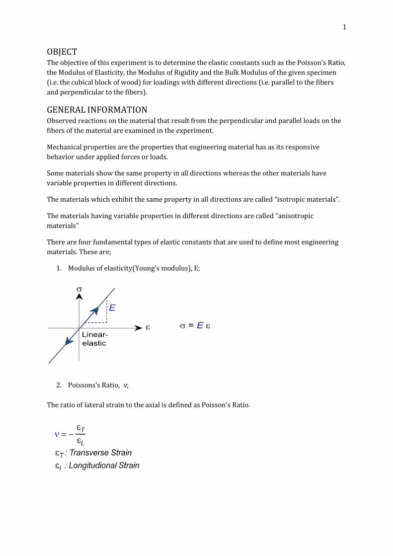
1. Modulus of elasticity(Young’s modulus), E;

2. Poissons’s Ratio, ν;

The ratio of lateral strain to the axial is defined as Poisson’s Ratio.

2

3. Bulk Modulus (modulus of compressibility),K;

The ratio of the hydrostatic pressure on the body to its volumetric strain is defined as “Bulk Modulus”.

4. Shear Modulus (Modulus of rigidity),G;

The ratio of shear stress to the shear strain is defined as “shear modulus”.

TEST SPECIMEN

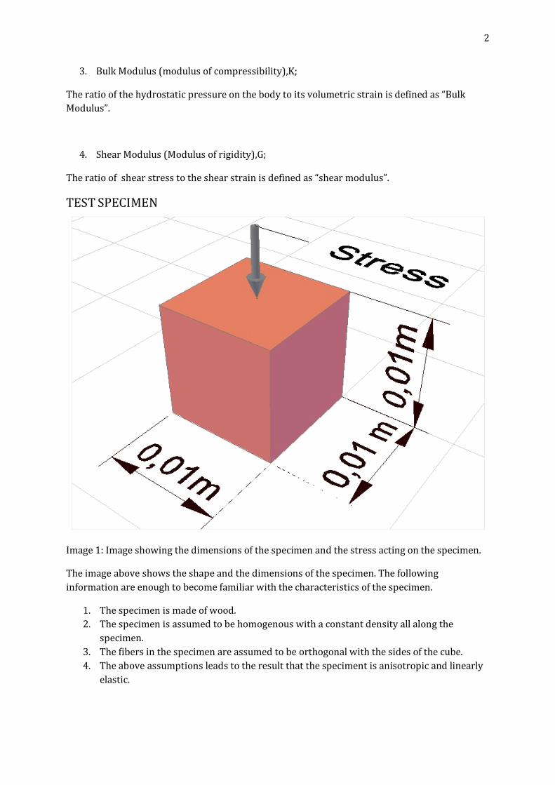
Image 1: Image showing the dimensions of the specimen and the stress acting on the specimen.

The image above shows the shape and the dimensions of the specimen. The following information are enough to become familiar with the characteristics of the specimen.

1. The specimen is made of wood. 2. The specimen is assumed to be homogenous with a constant density all along the

specimen. 3. The fibers in the specimen are assumed to be orthogonal with the sides of the cube. 4. The above assumptions leads to the result that the speciment is anisotropic and linearly

elastic.

3

APPARATUS The following apparatus are going to be used for the testing of the specimen.

• A universal testing machine (10 tons) • A dial gage with an accuracy of 1,00E-03” • A dial gage with an accuracy of 1,00E-04” • 4 cylindirical iron rods with the length of 0.3m and base diameter of 0,008m. • A cylindirical iron rod with a length of 0.2m and base diameter of 0,001m.

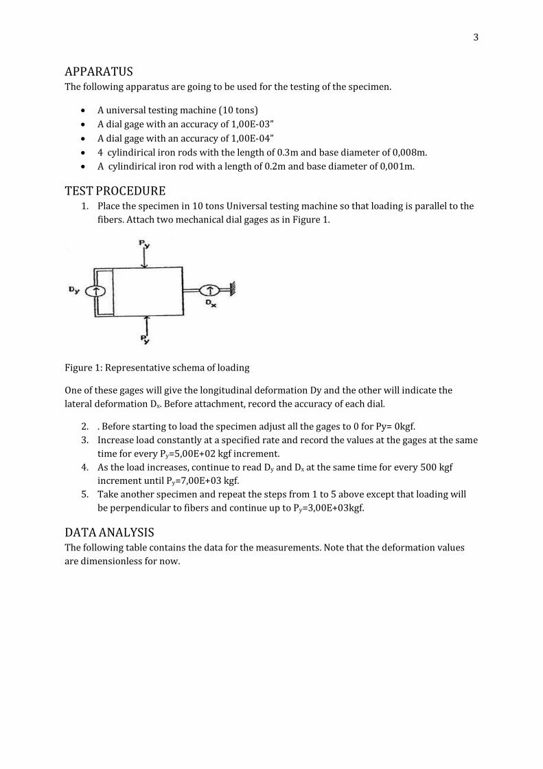
TEST PROCEDURE 1. Place the specimen in 10 tons Universal testing machine so that loading is parallel to the

fibers. Attach two mechanical dial gages as in Figure 1.

Figure 1: Representative schema of loading

One of these gages will give the longitudinal deformation Dy and the other will indicate the lateral deformation Dx. Before attachment, record the accuracy of each dial.

2. . Before starting to load the specimen adjust all the gages to 0 for Py= 0kgf. 3. Increase load constantly at a specified rate and record the values at the gages at the same

time for every Py=5,00E+02 kgf increment. 4. As the load increases, continue to read Dy and Dx at the same time for every 500 kgf

increment until Py=7,00E+03 kgf. 5. Take another specimen and repeat the steps from 1 to 5 above except that loading will

be perpendicular to fibers and continue up to Py=3,00E+03kgf.

DATA ANALYSIS The following table contains the data for the measurements. Note that the deformation values are dimensionless for now.

4

Force that is applied on the specimen - P (kgf)

Parallel Perpendicular Values measured by the transverse dial gage - Δx

Values measured by the axial dial gage - Δy

Values measured by the transverse dial gage – Δx

Values measured by the axial dial gage - Δy

0,00E+00 0,00E+00 0,00E+00 0,00E+00 0,00E+00 5,00E+02 1,50E+01 3,00E+00 8,00E+00 5,00E+01 1,00E+03 4,00E+01 2,10E+01 4,00E+01 8,00E+01 1,50E+03 5,00E+01 4,00E+01 8,00E+01 1,50E+02 2,00E+03 5,50E+01 5,10E+01 1,00E+02 2,30E+02 2,50E+03 6,40E+01 6,10E+01 1,05E+02 3,80E+02 3,00E+03 7,00E+01 7,10E+01 1,23E+02 5,10E+02 3,50E+03 7,50E+01 8,00E+01

- -

4,00E+03 8,30E+01 9,00E+01 4,50E+03 8,90E+01 9,10E+01 5,00E+03 9,30E+01 1,00E+02 5,50E+03 9,70E+01 1,01E+02 6,00E+03 9,80E+01 1,10E+02 6,50E+03 1,00E+02 1,20E+02 7,00E+03 1,03E+02 1,20E+02

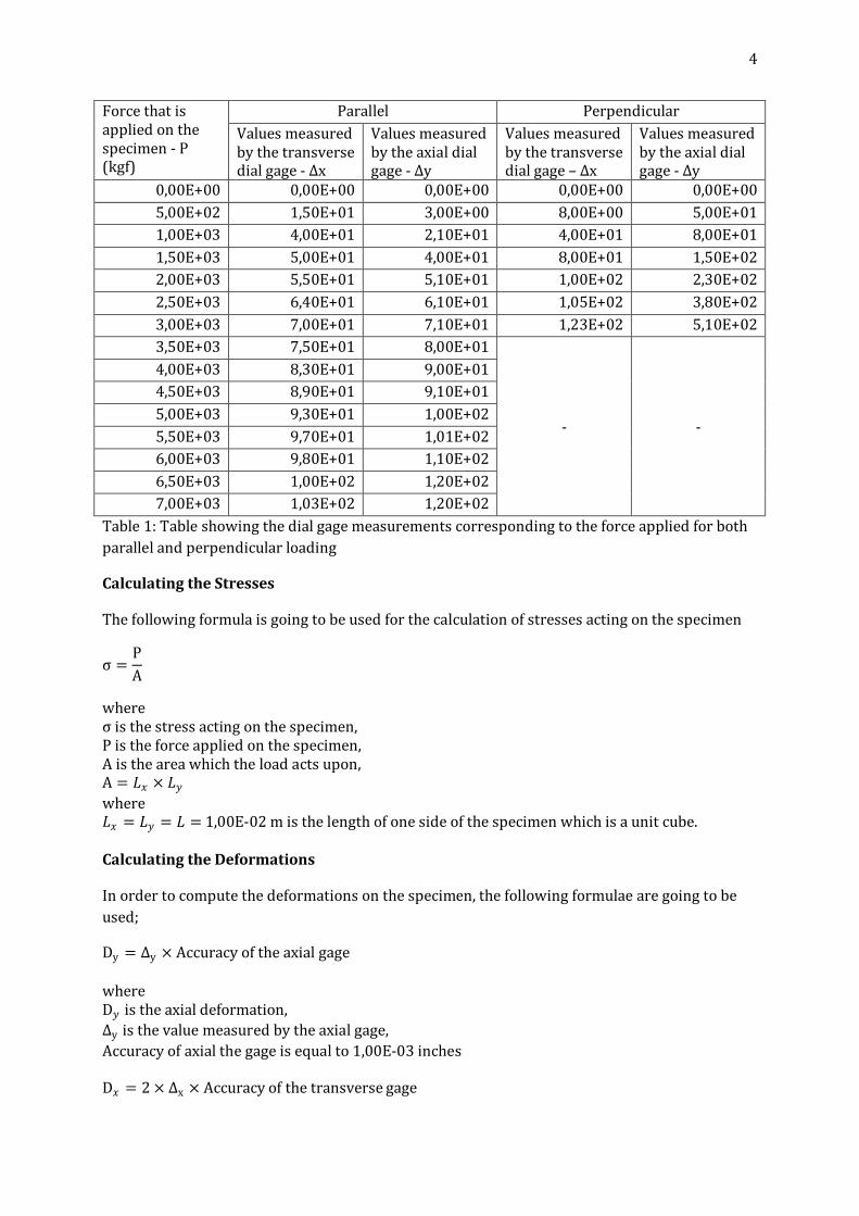
Table 1: Table showing the dial gage measurements corresponding to the force applied for both parallel and perpendicular loading

Calculating the Stresses

The following formula is going to be used for the calculation of stresses acting on the specimen

σ =PA

where σ is the stress acting on the specimen, P is the force applied on the specimen, A is the area which the load acts upon, A = 𝐿𝐿𝑥𝑥 × 𝐿𝐿𝑦𝑦 where 𝐿𝐿𝑥𝑥 = 𝐿𝐿𝑦𝑦 = 𝐿𝐿 = 1,00E-02 m is the length of one side of the specimen which is a unit cube.

Calculating the Deformations

In order to compute the deformations on the specimen, the following formulae are going to be used;

Dy = Δy × Accuracy of the axial gage

where D𝑦𝑦 is the axial deformation, Δy is the value measured by the axial gage, Accuracy of axial the gage is equal to 1,00E-03 inches D𝑥𝑥 = 2 × Δx × Accuracy of the transverse gage

5

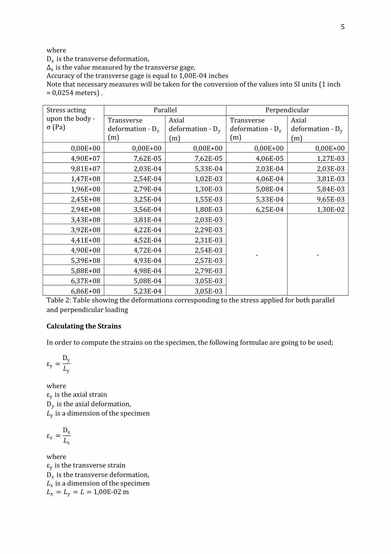
where D𝑥𝑥 is the transverse deformation, Δx is the value measured by the transverse gage, Accuracy of the transverse gage is equal to 1,00E-04 inches Note that necessary measures will be taken for the conversion of the values into SI units (1 inch = 0,0254 meters) . Stress acting upon the body - σ (Pa)

Parallel Perpendicular Transverse deformation - D𝑥𝑥 (m)

Axial deformation - D𝑦𝑦 (m)

Transverse deformation - D𝑥𝑥 (m)

Axial deformation - D𝑦𝑦 (m)

0,00E+00 0,00E+00 0,00E+00 0,00E+00 0,00E+00 4,90E+07 7,62E-05 7,62E-05 4,06E-05 1,27E-03 9,81E+07 2,03E-04 5,33E-04 2,03E-04 2,03E-03 1,47E+08 2,54E-04 1,02E-03 4,06E-04 3,81E-03 1,96E+08 2,79E-04 1,30E-03 5,08E-04 5,84E-03 2,45E+08 3,25E-04 1,55E-03 5,33E-04 9,65E-03 2,94E+08 3,56E-04 1,80E-03 6,25E-04 1,30E-02 3,43E+08 3,81E-04 2,03E-03

- -

3,92E+08 4,22E-04 2,29E-03 4,41E+08 4,52E-04 2,31E-03 4,90E+08 4,72E-04 2,54E-03 5,39E+08 4,93E-04 2,57E-03 5,88E+08 4,98E-04 2,79E-03 6,37E+08 5,08E-04 3,05E-03 6,86E+08 5,23E-04 3,05E-03

Table 2: Table showing the deformations corresponding to the stress applied for both parallel and perpendicular loading

Calculating the Strains

In order to compute the strains on the specimen, the following formulae are going to be used;

εy =Dy

𝐿𝐿y

where εy is the axial strain D𝑦𝑦 is the axial deformation, 𝐿𝐿y is a dimension of the specimen

ε𝑥𝑥 =Dx

𝐿𝐿x

where εy is the transverse strain D𝑥𝑥 is the transverse deformation, 𝐿𝐿x is a dimension of the specimen 𝐿𝐿𝑥𝑥 = 𝐿𝐿𝑦𝑦 = 𝐿𝐿 = 1,00E-02 m

6

Calculating Poisson’s Ratio for Each Stress Value

It is known that the Poisson’s Ratio becomes

ν =Δε𝑥𝑥Δε𝑦𝑦

for the specimen where ν is the Poisson’s Ratio for the specimen, ε𝑥𝑥 is the transverse strain, ε𝑦𝑦 is the axial strain. For each stress value. Therefore we would obtain it by dividing each transverse strain value by its corresponding axial strain value. It would then be necessary to take the arithmetic means of these values. The table below shows the results.

Stress acting upon the body - σ (Pa)

Parallel Perpendicular Transverse strain - ε𝑥𝑥

Axial strain - ε𝑦𝑦

Poisson’s Ratio - ν

Transverse strain - ε𝑥𝑥

Axial strain - ε𝑦𝑦

Poisson’s Ratio - ν

0,00E+00 0,00E+00 0,00E+00 0.00E+00 0,00E+00 0,00E+00 0.00E+00 4,90E+07 7,62E-03 7,62E-03 1.00E+00 4,06E-03 1,27E-01 3.20E-02 9,81E+07 2,03E-02 5,33E-02 3.81E-01 2,03E-02 2,03E-01 1.00E-01 1,47E+08 2,54E-02 1,02E-01 2.50E-01 4,06E-02 3,81E-01 1.07E-01 1,96E+08 2,79E-02 1,30E-01 2.16E-01 5,08E-02 5,84E-01 8.70E-02 2,45E+08 3,25E-02 1,55E-01 2.10E-01 5,33E-02 9,65E-01 5.53E-02 2,94E+08 3,56E-02 1,80E-01 1.97E-01 6,25E-02 1,30E+00 4.82E-02 3,43E+08 3,81E-02 2,03E-01 1.88E-01

- - -

3,92E+08 4,22E-02 2,29E-01 1.84E-01 4,41E+08 4,52E-02 2,31E-01 1.96E-01 4,90E+08 4,72E-02 2,54E-01 1.86E-01 5,39E+08 4,93E-02 2,57E-01 1.92E-01 5,88E+08 4,98E-02 2,79E-01 1.78E-01 6,37E+08 5,08E-02 3,05E-01 1.67E-01 6,86E+08 5,23E-02 3,05E-01 1.72E-01

Table 3: Table showing the strains corresponding to the stress applied for both parallel and perpendicular loading

Arithmetic mean of ν for parallel loading Arithmetic mean of ν for perpendicular loading 2.48E-01 6.13E-02

Table 4: Table showing the arithmetic mean of the Poisson’s Ratios for both parallel and perpendicular loading.

Calculating Poisson’s Ratio Through Linear Regression

It is known that;

ν =𝑑𝑑ε𝑥𝑥𝑑𝑑ε𝑦𝑦

for the specimen where ν is the Poisson’s Ratio for the specimen, ε𝑥𝑥 is the transverse strain,

7

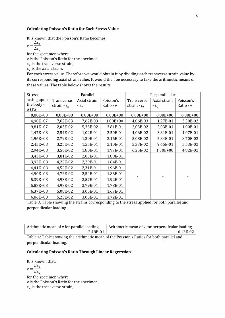
ε𝑦𝑦 is the axial strain. Assuming that the specimen is linearly elastic, linear regression would be feasible for calculating the Poisson’s Ratio where ν becomes;

ν =Δε𝑥𝑥Δε𝑦𝑦

Plotting the graphs;

Graph 3: ε𝑦𝑦 vs ε𝑥𝑥 graph for the parallel loading

It is observed from the graph that the Poisson’s Ratio for the parallel loading is, ν𝑝𝑝𝑝𝑝𝑝𝑝𝑝𝑝𝑝𝑝𝑝𝑝𝑝𝑝𝑝𝑝 =1,55E-01

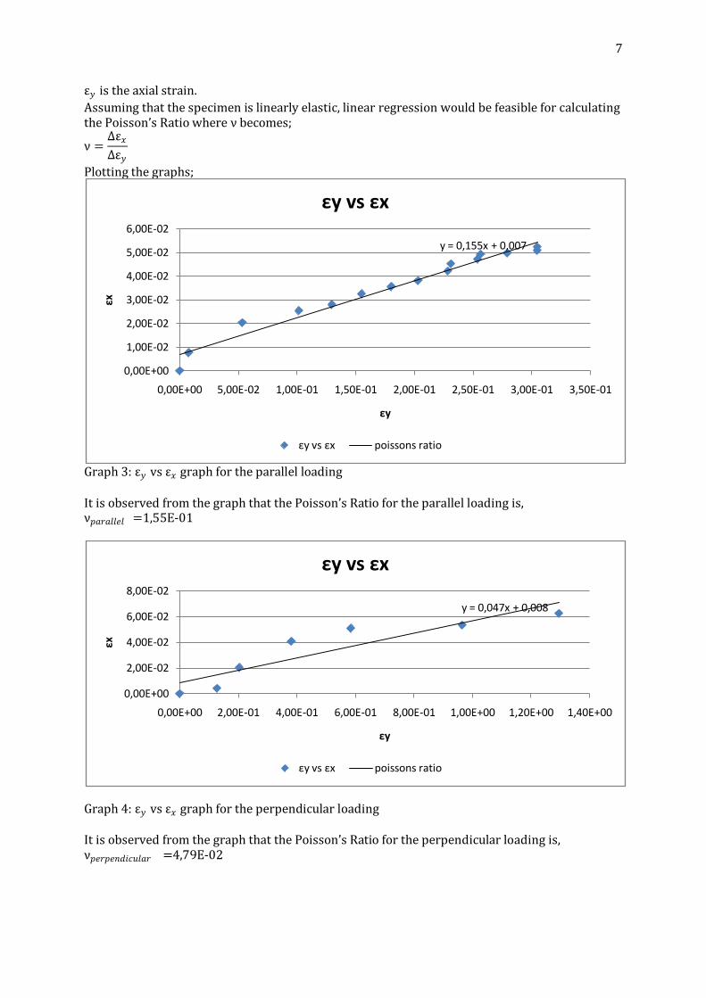
Graph 4: ε𝑦𝑦 vs ε𝑥𝑥 graph for the perpendicular loading

It is observed from the graph that the Poisson’s Ratio for the perpendicular loading is, ν𝑝𝑝𝑝𝑝𝑝𝑝𝑝𝑝𝑝𝑝𝑝𝑝𝑑𝑑𝑝𝑝𝑝𝑝𝑝𝑝𝑝𝑝𝑝𝑝𝑝𝑝 =4,79E-02

y = 0,155x + 0,007

0,00E+00

1,00E-02

2,00E-02

3,00E-02

4,00E-02

5,00E-02

6,00E-02

0,00E+00 5,00E-02 1,00E-01 1,50E-01 2,00E-01 2,50E-01 3,00E-01 3,50E-01

εx

εy

εy vs εx

εy vs εx poissons ratio

y = 0,047x + 0,008

0,00E+00

2,00E-02

4,00E-02

6,00E-02

8,00E-02

0,00E+00 2,00E-01 4,00E-01 6,00E-01 8,00E-01 1,00E+00 1,20E+00 1,40E+00

εx

εy

εy vs εx

εy vs εx poissons ratio

8

Calculating the Modulus of Elasticity

In order to find the Modulus of Elasticity of the specimen for both the parallel and perpendicular loadings, 𝐸𝐸𝑝𝑝𝑝𝑝𝑝𝑝𝑝𝑝𝑝𝑝𝑝𝑝𝑝𝑝𝑝𝑝 and 𝐸𝐸𝑝𝑝𝑝𝑝𝑝𝑝𝑝𝑝𝑝𝑝𝑝𝑝𝑑𝑑𝑝𝑝𝑝𝑝𝑝𝑝𝑝𝑝𝑝𝑝𝑝𝑝 , the following formula is going to be used assuming that the specimen is linearly elastic.

𝐸𝐸 =𝑡𝑡𝑝𝑝𝑝𝑝𝑡𝑡𝑝𝑝𝑝𝑝𝑝𝑝 𝑡𝑡𝑡𝑡𝑝𝑝𝑝𝑝𝑡𝑡𝑡𝑡𝑡𝑡𝑝𝑝𝑝𝑝𝑡𝑡𝑝𝑝𝑝𝑝𝑝𝑝 𝑡𝑡𝑡𝑡𝑝𝑝𝑝𝑝𝑝𝑝𝑝𝑝

=σε𝑦𝑦

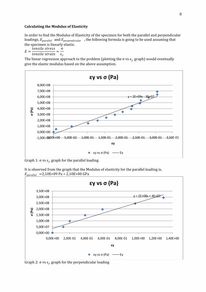
The linear regression approach to the problem (plotting the σ vs ε𝑦𝑦 graph) would eventually give the elastic modulus based on the above assumption.

Graph 1: σ vs ε𝑦𝑦 graph for the parallel loading

It is observed from the graph that the Modulus of elasticity for the parallel loading is, 𝐸𝐸𝑝𝑝𝑝𝑝𝑝𝑝𝑝𝑝𝑝𝑝𝑝𝑝𝑝𝑝𝑝𝑝 =2,10E+09 Pa = 2,10E+00 GPa

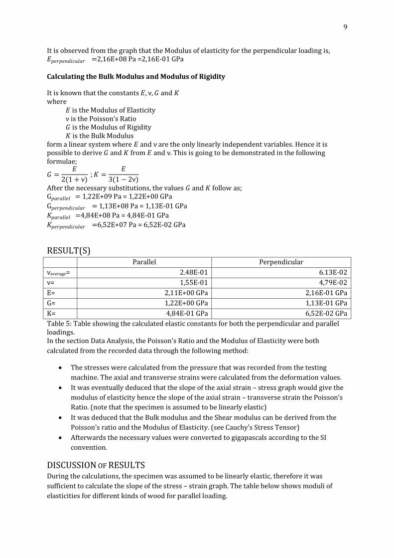
Graph 2: σ vs ε𝑦𝑦 graph for the perpendicular loading

y = 2E+09x - 3E+07

-1,00E+08

0,00E+00

1,00E+08

2,00E+08

3,00E+08

4,00E+08

5,00E+08

6,00E+08

7,00E+08

8,00E+08

0,00E+00 5,00E-02 1,00E-01 1,50E-01 2,00E-01 2,50E-01 3,00E-01 3,50E-01

σ (P

a)

εy

εy vs σ (Pa)

εy vs σ (Pa) Ey

y = 2E+08x + 4E+07

0,00E+00

5,00E+07

1,00E+08

1,50E+08

2,00E+08

2,50E+08

3,00E+08

3,50E+08

0,00E+00 2,00E-01 4,00E-01 6,00E-01 8,00E-01 1,00E+00 1,20E+00 1,40E+00

σ (P

a)

εy

εy vs σ (Pa)

εy vs σ (Pa) Ey

9

It is observed from the graph that the Modulus of elasticity for the perpendicular loading is, 𝐸𝐸𝑝𝑝𝑝𝑝𝑝𝑝𝑝𝑝𝑝𝑝𝑝𝑝𝑑𝑑𝑝𝑝𝑝𝑝𝑝𝑝𝑝𝑝𝑝𝑝𝑝𝑝 =2,16E+08 Pa =2,16E-01 GPa

Calculating the Bulk Modulus and Modulus of Rigidity

It is known that the constants 𝐸𝐸, ν,𝐺𝐺 and 𝐾𝐾 where

𝐸𝐸 is the Modulus of Elasticity ν is the Poisson’s Ratio 𝐺𝐺 is the Modulus of Rigidity 𝐾𝐾 is the Bulk Modulus

form a linear system where 𝐸𝐸 and ν are the only linearly independent variables. Hence it is possible to derive 𝐺𝐺 and 𝐾𝐾 from 𝐸𝐸 and ν. This is going to be demonstrated in the following formulae;

𝐺𝐺 =𝐸𝐸

2(1 + ν) ;𝐾𝐾 =

𝐸𝐸3(1 − 2ν)

After the necessary substitutions, the values 𝐺𝐺 and 𝐾𝐾 follow as; G𝑝𝑝𝑝𝑝𝑝𝑝𝑝𝑝𝑝𝑝𝑝𝑝𝑝𝑝𝑝𝑝 = 1,22E+09 Pa = 1,22E+00 GPa G𝑝𝑝𝑝𝑝𝑝𝑝𝑝𝑝𝑝𝑝𝑝𝑝𝑑𝑑𝑝𝑝𝑝𝑝𝑝𝑝𝑝𝑝𝑝𝑝𝑝𝑝 = 1,13E+08 Pa = 1,13E-01 GPa 𝐾𝐾𝑝𝑝𝑝𝑝𝑝𝑝𝑝𝑝𝑝𝑝𝑝𝑝𝑝𝑝𝑝𝑝 =4,84E+08 Pa = 4,84E-01 GPa 𝐾𝐾𝑝𝑝𝑝𝑝𝑝𝑝𝑝𝑝𝑝𝑝𝑝𝑝𝑑𝑑𝑝𝑝𝑝𝑝𝑝𝑝𝑝𝑝𝑝𝑝𝑝𝑝 =6,52E+07 Pa = 6,52E-02 GPa

RESULT(S) Parallel Perpendicular

νaverage= 2.48E-01 6.13E-02 ν= 1,55E-01 4,79E-02 E= 2,11E+00 GPa 2,16E-01 GPa G= 1,22E+00 GPa 1,13E-01 GPa K= 4,84E-01 GPa 6,52E-02 GPa Table 5: Table showing the calculated elastic constants for both the perpendicular and parallel loadings. In the section Data Analysis, the Poisson’s Ratio and the Modulus of Elasticity were both calculated from the recorded data through the following method:

• The stresses were calculated from the pressure that was recorded from the testing machine. The axial and transverse strains were calculated from the deformation values.

• It was eventually deduced that the slope of the axial strain – stress graph would give the modulus of elasticity hence the slope of the axial strain – transverse strain the Poisson’s Ratio. (note that the specimen is assumed to be linearly elastic)

• It was deduced that the Bulk modulus and the Shear modulus can be derived from the Poisson’s ratio and the Modulus of Elasticity. (see Cauchy’s Stress Tensor)

• Afterwards the necessary values were converted to gigapascals according to the SI convention.

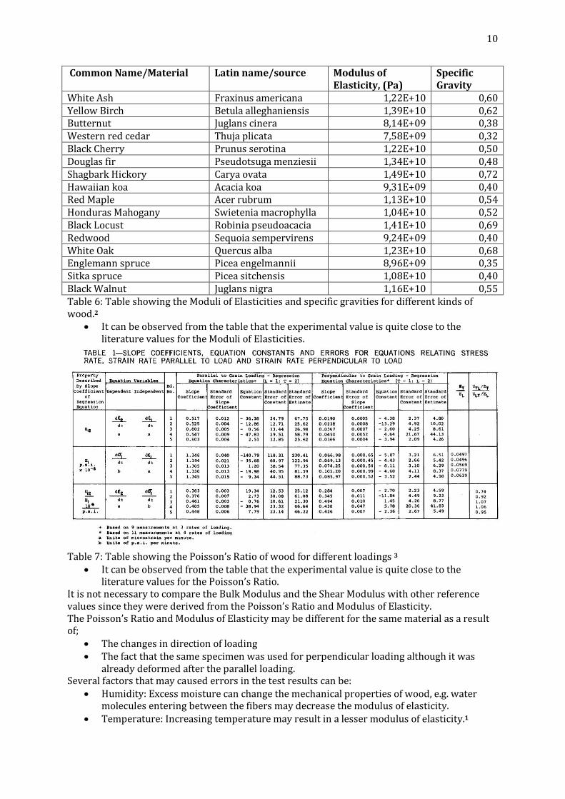
DISCUSSION OF RESULTS During the calculations, the specimen was assumed to be linearly elastic, therefore it was sufficient to calculate the slope of the stress – strain graph. The table below shows moduli of elasticities for different kinds of wood for parallel loading.

10

Common Name/Material Latin name/source Modulus of Elasticity, (Pa)

Specific Gravity

White Ash Fraxinus americana 1,22E+10 0,60 Yellow Birch Betula alleghaniensis 1,39E+10 0,62 Butternut Juglans cinera 8,14E+09 0,38 Western red cedar Thuja plicata 7,58E+09 0,32 Black Cherry Prunus serotina 1,22E+10 0,50 Douglas fir Pseudotsuga menziesii 1,34E+10 0,48 Shagbark Hickory Carya ovata 1,49E+10 0,72 Hawaiian koa Acacia koa 9,31E+09 0,40 Red Maple Acer rubrum 1,13E+10 0,54 Honduras Mahogany Swietenia macrophylla 1,04E+10 0,52 Black Locust Robinia pseudoacacia 1,41E+10 0,69 Redwood Sequoia sempervirens 9,24E+09 0,40 White Oak Quercus alba 1,23E+10 0,68 Englemann spruce Picea engelmannii 8,96E+09 0,35 Sitka spruce Picea sitchensis 1,08E+10 0,40 Black Walnut Juglans nigra 1,16E+10 0,55 Table 6: Table showing the Moduli of Elasticities and specific gravities for different kinds of wood.2

• It can be observed from the table that the experimental value is quite close to the literature values for the Moduli of Elasticities.

Table 7: Table showing the Poisson’s Ratio of wood for different loadings 3

• It can be observed from the table that the experimental value is quite close to the literature values for the Poisson’s Ratio.

It is not necessary to compare the Bulk Modulus and the Shear Modulus with other reference values since they were derived from the Poisson’s Ratio and Modulus of Elasticity. The Poisson’s Ratio and Modulus of Elasticity may be different for the same material as a result of;

• The changes in direction of loading • The fact that the same specimen was used for perpendicular loading although it was

already deformed after the parallel loading. Several factors that may caused errors in the test results can be:

• Humidity: Excess moisture can change the mechanical properties of wood, e.g. water molecules entering between the fibers may decrease the modulus of elasticity.

• Temperature: Increasing temperature may result in a lesser modulus of elasticity.1

11

• Specific gravity: Specific gravity of the wood specimen used in the test may be different than that of the literature value.

• Mechanical Properties: Fibers in the wood may not be perfectly linear or orthogonal as assumed.

• Apparatus: The dial gages may have different accuracies than expected and result in erroneous results.

• Human factor: Lack of caution in the experimenter’s actions may hava caused an error in the test results.

The condition of the specimen being anisotropic required data for two different directions of loading, one being aligning the fibers perpendicular to the loading and the other being aligning the fibers in a parallel fashion. The fibers could resist more in the parallel loading, since it was harder to compress parallel fibers stacked closely. The transverse deformation was multiplied with two since the apparatus was designed to measure the deformation from only one side.

CONCLUSION The objective of this test was to determine some elastic constants of wood. It was observed at the end of the calculations that the results were close to the literature values.

REFERENCES 1 Young Modulus of Elasticity for Metals and Alloys - Elastic properties and Youngs

modulus for common metals and alloys as cast iron, carbon steel and more (http://www.engineeringtoolbox.com/young-modulus-d_773.html)

2 Static Measurement of Young's Modulus along Grain (http://www.ukuleles.com/Technology/woodprop.html)

3 Silker, Alan. "Measuring Poisson's ratios in wood." Experimental Mechanics. Volume 12, Number 5, 239-242, DOI: 10.1007/BF02318105 .