determination of flow regimes in bubble columns...
TRANSCRIPT
DETERMINATION OF FLOW REGIMES IN BUBBLE COLUMNS USING CFD
A Thesis
Submitted of the College of Engineering
Of Nahrain University in Partial
Fulfillment of the Requirements for
the Degree of Master of Science in
Chemical Engineering
by
Rana Rasool Jaleel
(B.Sc. in Chemical Engineering 2005)
Muharram 1430
January 2009
I
ABSTRACT
Computational fluid dynamics (CFD) simulation, deals with the solution of
fluid dynamic equations on digital computers, requiring relatively few
restrictive assumptions and thus giving a complete description of the
hydrodynamics of bubble columns. This detailed predicted flow field gives an
accurate insight to the fluid behaviors.
3D simulation computational fluid dynamics (CFD) is applied using
ANSYS-CFX Euler-Euler model to measure the hydrodynamic of an airlift
reactor, and comparing with experimental data of Baten et. al., (1999). Also
by comparing the hydrodynamics of airlift reactor within bubble column
reactor, of air/water and in the homogeneous bubble flow regime, it can be
noticed that the liquid circulation velocities are more significant in the airlift
configuration than in bubble columns, leading to significantly lower gas
holdups. Within the riser of the airlift, the gas and liquid phases are virtually
in plug flow, whereas in bubble column the gas and liquid phases follow
parabolic velocity distribution. The transition regime appears at high
superficial gas velocity in airlift reactors because of its ability to operate in
the homogeneous bubble flow regime till much higher superficial gas
velocities.
II
CONTENTS
Abstract І
Contents П
Notations
List of Tables
List of Figures
ІV
VI
VII
Chapter One: Introduction 1.1 Bubble Column
1.2 Computational Fluid Dynamics (CFD)
1.2.2 Performance of CFD
1.2.3 Flow & Mixing Applications of CFD
1.2.4 Parameters of CFD
1.3 Aim of the work
1
2
4
6
6
7
Chapter Two: Literature Survey 2.1 Gas Holdup
2.2 Axial Liquid Velocities
2.3 Numeric Simulation in Fluids
8
10
11
2.4 Transition Regime 15
Chapter Three: Theoretical Aspect3.1 Hydrodynamics in Bubble Column and Airlift Reactor
3.2 Factors Influencing Hydrodynamics of Bubble Column Reactors
3.3 Flow Regime
3.3.1 Homogenous Flow
3.3.2 Heterogeneous Flow
3.3.2.1 Churn-Turbulent Flows
3.3.2.2 Slug Flow
18
18
22
22
23
23
23
III
3.4 Bubble Formation
3.5 Bubble Coalescence and Break-up
3.6 Bubbles Motion
3.7 Relationship between the Riser and Downcomer Gas Holdup in Airlift
Reactors
3.8 Axial Liquid Velocity
3.9 Transition Regime
24
24
26
26
33
32
33
Chapter Four: Results and Discussion 4.1 Computational Fluid Dynamics (CFD) Simulation
4.2 Computing Technology
4.3 Development of CFD Model
4.4 Simulation Results
4.5 Mechanism of Flow in Airlift Reactors
4.6 Radial Distribution
4.7 Transition Velocity
4.8 Transition Regime Identification Using the Drift Flux Plot 4.9 Comparisons between the Hydrodynamics in the Airlift Reactor with
Bubble Columns
36
36
37
39
46
49
51
52
53
Chapter Five: Conclusions and Recommendation for Future Work
5.1 Conclusions 58
5.2 Recommendations for future work 59
References 60
Appendix "A" A-1
Appendix "B" B-1
Appendix "C" C-1
IV
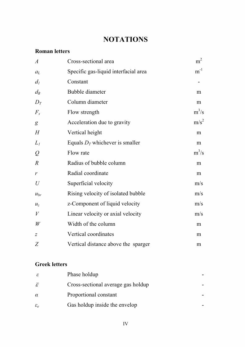
NOTATIONS
Roman letters
A Cross-sectional area m2
aL Specific gas-liquid interfacial area m-1
d1 Constant -
dB Bubble diameter m
DT Column diameter m
Fs Flow strength m3/s
g Acceleration due to gravity m/s2
H Vertical height m
L1 Equals DT whichever is smaller m
Q Flow rate m3/s
R Radius of bubble column m
r Radial coordinate m
U Superficial velocity m/s
ubr Rising velocity of isolated bubble m/s
uz z-Component of liquid velocity m/s
V Linear velocity or axial velocity m/s
W Width of the column m
z
Z
Vertical coordinates
Vertical distance above the sparger
m
m
Greek letters
ε Phase holdup -
ε Cross-sectional average gas holdup -
α Proportional constant -
εe Gas holdup inside the envelop -
V
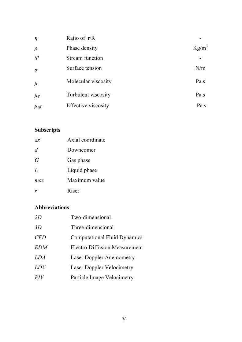
η Ratio of r/R -
ρ Phase density Kg/m3
Ψ Stream function -
σ Surface tension
N/m
µ Molecular viscosity Pa.s
µT Turbulent viscosity Pa.s
µeff Effective viscosity Pa.s
Subscripts
ax Axial coordinate
d Downcomer
G Gas phase
L Liquid phase
max Maximum value
r Riser
Abbreviations
2D Two-dimensional
3D Three-dimensional
CFD Computational Fluid Dynamics
EDM Electro Diffusion Measurement
LDA Laser Doppler Anemometry
LDV Laser Doppler Velocimetry
PIV Particle Image Velocimetry
VI
List of Tables Table Title Page(3.1) Interrelationship between the riser and the downcomer gas
holdups in airlift reactors:
29
(4.1) Local and average gas holdup and liquid velocity in riser and
downcomer at 0.018634 m/s superficial gas velocity
40
(4.2) Local and average gas holdup and liquid velocity in riser and
downcomer at 0.040887m/s superficial gas velocity
41
(4.3) Local and average gas holdup and liquid velocity in riser and
downcomer at 0.056583 m/s superficial gas velocity
42
(4.4) Local and average gas holdup and liquid velocity in riser and
downcomer at 0.081263 m/s superficial gas velocity
43
(4.5) Local and average gas holdup and liquid velocity in riser and
downcomer at 0.094986 m/s superficial gas velocity
44
(4.5) Local and average gas holdup and liquid velocity in riser and
downcomer at 0.11419193 m/s superficial gas velocity
45
VII
List of Figures Table Title Page(1.1) Performance Targets for Computational Fluid Dynamics. 5
(2.1) Three snapshots of the iso-surface of the bubble plume, the
surface indicates (εG = 0.1). The liquid velocity field in the centre
plane is also shown. The plots are respectively 100, 200 and 300s
after the start of the simulation.
12
(2.2) Effect of liquid static height on transition velocity. 15
(2.3) Effect of column diameter on transition velocity. 16
(3.1) Flow regimes encountered in bubble columns (Urseanu and
Krishna, 2000).
19
(3.2) Flow regimes based on superficial velocity and column diameter
(Urseanu and Krishna, 2000).
19
(3.3) Schematic representation of equation (3.10). 32
(3.4) Typical drift flux plot using Wallis (1969) apporach (Deckwer et
al., 1981).
34
(4.1) Schematic of airlift reactor, showing the computational domains
and grid details.
38
(4.2) Contours of air volume fraction and liquid velocity at 0.018634
m/s superficial gas velocity.
40
(4.3) Contours of air volume fraction and liquid velocity at
0.040887m/s superficial gas velocity.
41
(4.4) Contours of air volume fraction and liquid velocity at 0.056583
m/s superficial gas velocity.
42
(4.5) Contours of air volume fraction and liquid velocity at 0.081263
m/s superficial gas velocity.
43
(4.6) Contours of air volume fraction and liquid velocity at 0.094986
m/s superficial gas velocity.
44
(4.7) Contours of air volume fraction and liquid velocity at
0.11419193 m/s superficial gas velocity.
45
(4.8a) Comparison of airlift experimental data of Van Baten et 47
VIII
al.(1999) with CFD simulations for average gas holdup in the
riser.
(4.8b) Comparison of airlift experimental data of Van Baten et
al.(1999) with CFD simulations for average liquid velocity in the
riser.
47
(4.8c) Comparison of airlift experimental data of Van Baten et
al.(1999) with CFD simulations for average liquid velocity in the
downcomer.
48
(4.9a) Radial distribution of Gas holdup , for varying superficial gas
velocity, at height 1.75m above the sparger.
50
(4.9b) Radial distribution of liquid velocity in riser and downcomer, for
varying superficial gas velocity, at height 1.75m above the
sparger.
50
(4.10) Effect of gas velocity on the axial liquid velocity at column
center.
51
(4.11) Identification of flow regime transition based on drift-flux
method.
52
(4.12) Effect of superficial gas velocity on the gas hold-up in riser of
airlift reactor (UG,trans = 0.0899 m/s).
53
(4.13a) Comparison of gas holdup, for airlift reactor with bubble column
of 0.15 m diameter.
54
(4.13b) Comparison of centerline liquid velocity, VL(0), for airlift reactor
with bubble column of 0.15 m diameter.
54
(4.14) Identification of flow regime transition based on drift-flux
method in bubble column of 0.15 m diameter.
55
(4.15) Effect of superficial gas velocity on the gas hold-up in riser of
bubble column of diameter 0.15 m (UG,trans = 0.04 m/s).
56
1
CHAPTER ONE
INTRODUCTION
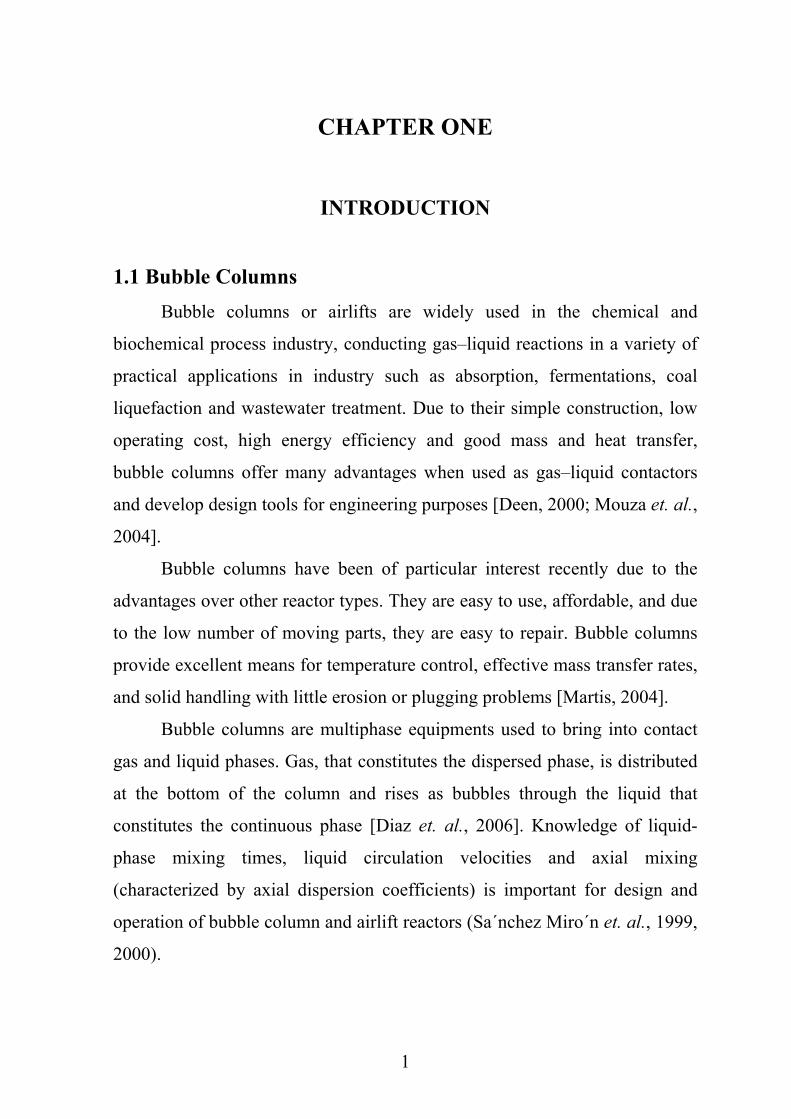
1.1 Bubble Columns Bubble columns or airlifts are widely used in the chemical and
biochemical process industry, conducting gas–liquid reactions in a variety of
practical applications in industry such as absorption, fermentations, coal
liquefaction and wastewater treatment. Due to their simple construction, low
operating cost, high energy efficiency and good mass and heat transfer,
bubble columns offer many advantages when used as gas–liquid contactors
and develop design tools for engineering purposes [Deen, 2000; Mouza et. al.,
2004].
Bubble columns have been of particular interest recently due to the
advantages over other reactor types. They are easy to use, affordable, and due
to the low number of moving parts, they are easy to repair. Bubble columns
provide excellent means for temperature control, effective mass transfer rates,
and solid handling with little erosion or plugging problems [Martis, 2004].
Bubble columns are multiphase equipments used to bring into contact
gas and liquid phases. Gas, that constitutes the dispersed phase, is distributed
at the bottom of the column and rises as bubbles through the liquid that
constitutes the continuous phase [Diaz et. al., 2006]. Knowledge of liquid-
phase mixing times, liquid circulation velocities and axial mixing
(characterized by axial dispersion coefficients) is important for design and
operation of bubble column and airlift reactors (Sa´nchez Miro´n et. al., 1999,
2000).
2
Bubble column hydrodynamics is complex and characterized by
different flow patterns depending on gas superficial velocity, liquid phase
properties, sparger design, column diameter etc. Non uniform gas hold-up
distribution within the vessel induces density fluctuations which originate
circulation currents influencing strongly phase mixing and transfer parameters
[Marchot et. al., 2001].
Gas holdup and liquid circulation velocity are amongst the most widely
studied parameters in airlift reactors. This emphasis attests to their
significance. The difference in gas holdup between the riser and the down
comer in an airlift reactor determines the magnitude of the induced liquid
circulation velocity which in turn influences the bubble rise velocity, and the
gas holdup. The holdup and the liquid velocity together affect the mixing
behavior, mass and heat transfer, the prevailing shear rate, and the ability of
the reactor to suspended solids. Clearly, all aspects of performance of airlift
systems are influenced by gas holdup and liquid circulation [Chisti et. al.,
1998].
1.2 Computational Fluid Dynamics (CFD) The numeric simulation in Fluid Mechanics and Heat and Mass
Transfer, commonly known as CFD “Computational Fluid Dynamics”, has an
expressive development in the last 20 years as a tool for physical problem
analyses in scientific investigations, and nowadays as a powerful tool in
solving important problems applied to engineering CFD permits a detailed
investigation of local effects of different types of equipment, such as chemical
and electrochemical reactors, heat exchangers, mixing tanks, cyclones,
combustion systems, among others [Silva et. al.,2005].
3
CFD can be regarded as an effective tool to clarify the importance of
physical effects (e.g. gravity, surface tension) on flow by adding or removing
them at will. An increasing number of papers deals with CFD application to
bubble columns [Wild et. al., 2003; Joshi, 2002]. Wild et. al., (2003) cite the
most important reasons for this increasing interest:
1. Measuring techniques applied to the local hydrodynamics in bubble
columns made huge progresses so that more reliable local
measurements are now available to check the adequacy of CFD
predictions.
2. Increased computer capacity.
3. The quality of the different CFD program systems has been improved:
better numerical methods, more realistic closure laws.
4. The occurrence of flow regimes, of deformable gas-liquid interfaces
and the lack of knowledge about the closure terms (turbulence, bubble-
bubble interactions) have transformed bubble column studies into a
benchmark of all gas-liquid dispersed flows.
For the numerical computation of two-phase flows two approaches are
mainly applied, namely the Euler/Euler and the Euler/Lagrange approach. The
first method considers both phases as interacting continua, while in the second
method the discrete nature of the dispersed phase is taken into account by
tracking a large number of individual bubbles through the flow field [Lain et.
al., 2000].
4
1.2.2 Performance of CFD
By predicting a system's performance in various areas, CFD can
potentially be used to improve the efficiency of existing operating systems as
well as the design of new systems. It can help to shorten product and process
development cycles, optimize processes to improve energy efficiency and
environmental performance, and solve problems as they arise in plant
operations. Also advances in CFD possible for the chemical and other low-
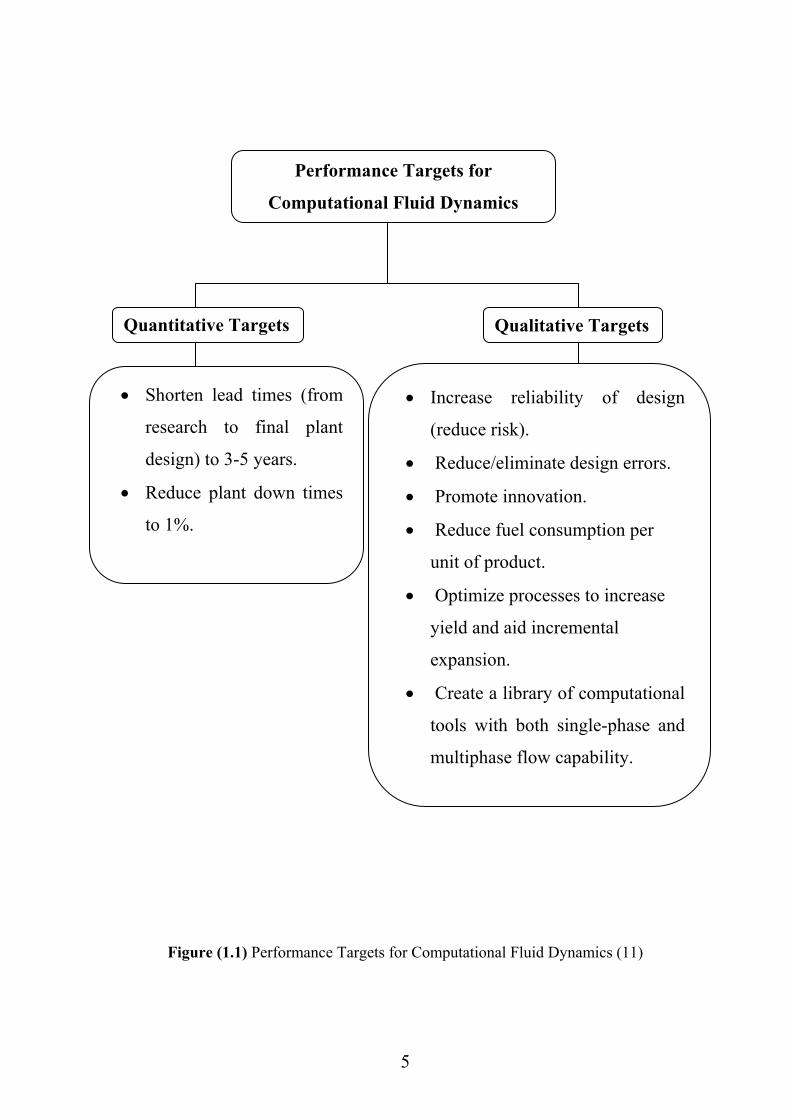
temperature process industries. With these broad goals as a base, specific
performance targets (both quantitative and qualitative) have been identified
for CFD, as shown in fig. (1.1). These targets illustrate how improvements in
computational fluid dynamics can have a wide- reaching impact throughout
the entire chemical industry.
The impact of CFD on the process and product development cycle is
greatest in the earliest phases (i.e., experimental optimization and scale-up).
CFD facilitates the design process by increasing the reliability of the design,
reducing or eliminating design errors, and allowing developers to visualize
the results of a process design or innovation. It promotes innovation by
making the design process shorter, less risky, and easier to accomplish. Using
CFD to resolve problems with existing processes can reduce equipment
failures and minimize poor operational performance, decreasing process shut-
down time. When used to optimize plant and equipment operation, CFD can
increase yields, providing a mechanism for incremental expansion.
5
Performance Targets for
Computational Fluid Dynamics
Quantitative Targets Qualitative Targets
• Shorten lead times (from
research to final plant
design) to 3-5 years.
• Reduce plant down times
to 1%.
• Increase reliability of design
(reduce risk).
• Reduce/eliminate design errors.
• Promote innovation.
• Reduce fuel consumption per
unit of product.
• Optimize processes to increase
yield and aid incremental
expansion.
• Create a library of computational
tools with both single-phase and
multiphase flow capability.
Figure (1.1) Performance Targets for Computational Fluid Dynamics (11)
6
1.2.3 Flow and Mixing Applications of CFD
1. Application model development.
2. Process and equipment optimizations, e.g. process yield, crystallizes,
reactors.
3. Reactor design (STR, bubble column, static and rotor-stator mixers).
4. Process and reactor scale up.
5. Parameter sensitivity studies.
6. Temperature control strategies.
7. Monomer/initiator dosing strategies.
8. Equipment rating.
9. Troubleshoot existing design problems.
10. Evaluate retrofit options.[49]
1.2.4 Parameters of CFD
1. Velocity and turbulence fields.
2. Concentrations of reactants, products and by-products.
3. Product distribution.
4. Temperature profiles.
5. Gas hold up.
6. Particle size/chain length distributions.
7. Solids distributions.
8. Batch time.
9. Residence time distribution.
10. Power draw Mix times.
11. Heat transfer coefficient [49].
7
1.3 Aim of the Work: This work is contributed in computational modeling studies of
multiphase flows in process and oil industry. It is a necessary start with
utmost attention being paid to numerical and physical fundamentals, which
can be easily extended to analyze other multiphase flow reactors, like
fluidized bed and bubble or slurry bubble columns. The main objectives of
this work are:
Using computational fluid dynamic (CFD) as a tool to:
1. Measuring of some the hydrodynamics of airlift reactor, and comparing
the results with experimental data.
2. Measuring transition liquid velocity and gas holdup in airlift reactor.
3. Comparing the hydrodynamic of airlift reactor with bubble column.
4. Measuring transition regimes for bubble column.
8
CHAPTER TWO
LITERATURE SURVEY
2.1 Gas Holdup Gas holdup and liquid circulation velocity are amongst the most widely
studied parameters in airlift reactors and bubble column. It can be defined as
the percentage by volume of the gas in the two or three phase in the column.
Vatai and Tekic (1989) investigated the effect of the column diameter
on the gas-holdup in bubble columns with pseudo plastic liquids. The
influence of the superficial gas velocity, physical properties of liquids and
column diameter (0.05, 0.1 and 0.2m) on the gas-holdup. They found that in
the investigated range of the superficial gas velocity the column diameter has
no influence on the gas-holdup in air-water system, and for high liquid
viscosity the column diameter effected a change in the gas-holdup. In a small-
diameter column large bubbles are stabilized by the column wall, which leads
to transition to slug flow regime and an increase in the gas-holdup.
Shun and Yasuhiro (1990) investigates experimentally by using
impulse response method, gas phase dispersion in bubble columns of 0.5 and
0.2m diameter at superficial gas velocities in the range 0.029-0.456 m/s.
Based on the recirculation theory of bubble columns, expression for the axial
dispersion coefficient of the gas phase was found: 23
TGG DU)180( αε = … (2.1)
where this equation quantatively describe the experimental results with the
proportional constant 9=α . At gas velocity higher than 0.1m/s, the gas phase
9
dispersion was suppressed by the insertion of perforated plate with a free of
44%.
Nenes et. al. (1994) presented analysis of real field data collected from
experiments on the outflow rate of the airlift pump, and a differential, two-
phase hydrodynamic model for the simulation of airlift pumps. Predictions
were obtained both by the hydrodynamic model and a mean air-volume
fraction model, and compared with real field experimental data. Both models
predicted correctly the overall behavioral trend of the experiments. However,
they were shown that the predictions based on the hydrodynamic model were,
in all cases, significantly better in comparison to the mean void fraction
model. This is because the hydrodynamic model takes into account the gas
compressibility itself (in the momentum and continuity equations) and all the
effects that result from this (i.e., multiple flow regimes). The mean air-volume
fraction model might give better predictions if a single flow regime were
predominant along the up riser. However, for water wells of moderate to large
depths, the compressibility effects of the gas phase are large, which among
other things leads to multiple flow regimes.
Ursula, Hans (2004) performs tracer experiments (jump responses) both
experimentally and also numerically. In both cases resulting data is then
analyzed with the aid of the convection-dispersion models that the integral
quantities gas hold-up, axial dispersion coefficient and mean residence time
show sufficient sensitivity with respect to the accuracy with which the
physical properties of the bubble column and the fluid flow are captured by
the computational grid, the boundary conditions and the sub-models for
interfacial momentum exchange.
Delmas et. al. (2006) performed investigation of local hydrodynamics
in a pilot plant bubble column using various techniques, exploring both axial
and radial variations of the gas hold-up, bubble average diameter and
10
frequency, surface area. Explored up a wide range of operating conditions to
large gas and liquid flow rates, with two sparger types. They found that very
strong effect of liquid flow on bubble column hydrodynamics at low gas flow
rate. First the flow regime map observed in batch mode is dramatically
modified with a drastic reduction of the homogeneous regime region, up to a
complete heterogeneous regime in the working conditions (UG> 0.02 m/s). On
the contrary, liquid flow has limited effects at very high gas flow rates.
2.2 Axial Liquid Velocities Viswanathan et. al., (1983) developed the mathematical model based
on the force balance to estimate circulation in cylindrical columns. The model
gave axial and radial variation of axial liquid velocity as a function of flow
strength. Flow strength equation is:
2d
1
3br
23
G31
br211s uRb
ULguLdF ⎥⎦
⎤⎢⎣
⎡= … (2.2)
The axial and radial variation of axial liquid velocity is:
⎟⎟⎠
⎞⎜⎜⎝
⎛−
=∂∂
−= ==
1e21
2
0re
0zz Lzsin
)1(LA2
rr)1(1u π
επψ
ε … (2.3)
and
[ ]6422avgz 92.032.36.01
RA2.1u ηηη −−+=⋅ … (2.4)
The analytical expressions derived analytical expressions for estimating the
flow strength besides simplifying calculation provides.
11
2.3 Numerical Simulation in Fluid Solbakken and Hjertager (1998) demonstrate CFD as a tool for scale up
of bubble column an industrial full-scale fermentation bubble column.
Bohn (2000) used 3D simulation of bubble column; gas holdup was
calculated by plotting the distribution of gas volume fraction vs. column
height. The plot showed a point where the concentration of gas increased
rapidly which is the gas-liquid interface. The next step was to compare the
height of liquid gas interface to the original height of liquid height interface.
The expansion, or amount of liquid gas interface rose, showed how much gas
holdup in the reactor, from which the gas holdup is easily calculated.
Michele (2001) presented the Electro Diffusion Measurement
technique (EDM) and computational results inside the 0.63 m diameter, 6 m
high bubble column and show that only a reasonable combination of these
two approaches can deliver new insights into physical phenomena and finally
yield tools helpful in reactor design and scale-up. Measurement results of
local dispersed phase holdups and liquid velocities delivered a strong
foundation for CFD model development and verification documenting
possibilities and limitations of implemented modeling strategies.
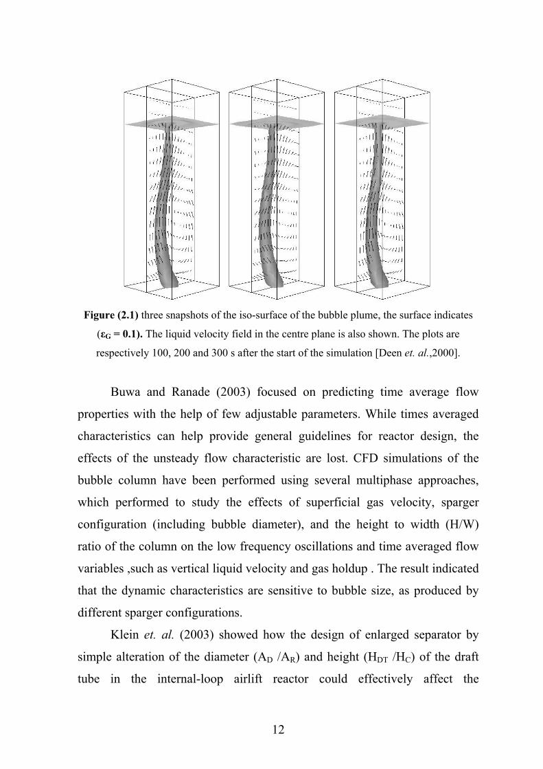
Deen et. al. (2000) used the commercial code CFX 4.3 to simulate the
gas-liquid flow in 3D rectangular bubble columns. The movement of a bubble
plume in a 3D bubble column was also simulated fig. (2.1). In contrary to the
other case only little temporal behavior was found. This disagrees with the
strongly time dependent flow, which was observed experimentally. In the
simulation the bubble plume moves into one corner and stays there for the rest
of the simulation time. This resulted in asymmetric velocity profiles. The
velocity profiles are better predicted higher up in the column.
12
Figure (2.1) three snapshots of the iso-surface of the bubble plume, the surface indicates
(εG = 0.1). The liquid velocity field in the centre plane is also shown. The plots are
respectively 100, 200 and 300 s after the start of the simulation [Deen et. al.,2000].
Buwa and Ranade (2003) focused on predicting time average flow
properties with the help of few adjustable parameters. While times averaged
characteristics can help provide general guidelines for reactor design, the
effects of the unsteady flow characteristic are lost. CFD simulations of the
bubble column have been performed using several multiphase approaches,
which performed to study the effects of superficial gas velocity, sparger
configuration (including bubble diameter), and the height to width (H/W)
ratio of the column on the low frequency oscillations and time averaged flow
variables ,such as vertical liquid velocity and gas holdup . The result indicated
that the dynamic characteristics are sensitive to bubble size, as produced by
different sparger configurations.
Klein et. al. (2003) showed how the design of enlarged separator by
simple alteration of the diameter (AD /AR) and height (HDT /HC) of the draft
tube in the internal-loop airlift reactor could effectively affect the
13
hydrodynamics of three-phase flow in the airlift reactor. The results showed
similar solids distribution in the riser and down comer; however, uniform
distribution was achieved only at higher gas flow rates. A very low solids
holdup in the enlarged separator zone was found, this parameter showing a
low sensitivity to changes of the air flow rate. The observations lead to the
conclusion that an airlift reactor with dual separator and an AD/AR ratio
around 1.2-2.0 can be suitable for batch/continuous high cell density systems,
where uniform solids distribution, an efficient separation of particles from the
liquid phase (upper part of the separator zone), and the maintenance of the
bubbles inside the reactor (narrow part) is desirable. In addition, the lower
part of the dual separator acts as an efficient mixer, which can significantly
help to improve the overall mixing in the airlift reactor. A three-phase fluid
model was used to predict the hydrodynamic parameters liquid velocity, gas
holdup and solids distribution data. It was shown that the model could.
Satisfactorily describe the behavior of a three-phase airlift reactor with a
significantly enlarged head zone, if the solids distribution between the
separator and the riser/down comer zones is known. The results of this study
coupled with the model predictions may be applied to suggest optimal design
(in terms of hydrodynamic behavior) of a batch/continuous three-phase airlift
reactor for high cell density fermentations.
Gobby and Hamill (2003) demonstrated the progress that has been
made in the modeling of complex multi-phase flows. In particular, the use of
coupled solvers for the Multi-Phase flows, together with features such as the
Population Balance Models and Generalized Grid Interfaces, is enabling the
incorporation of more realistic physical models, much more quickly than in
previous generations of CFD software.
Vladimir and Andrei (2003) presents the results of computational fluid
dynamics (CFD) modeling of gas liquid flows in water electrolysis systems.
14
CFD is used as a cost-effective design tool to optimize the performance of
different water electrolysis units. CFD software is used as a framework for
analyzing the gas-liquid flow characteristics (pressure, gas and liquid
velocities, gas and liquid volume fraction). The analysis is based on solving
the couple two-fluid conservation equations under typical and alternative
operating conditions with appropriate boundary conditions, turbulence models
and constitutive inter-phase correlations. Numerical results have been
validated based on the experimental available for a low-pressure data cell.
Mouza et. al. (2004) motivated by the need to develop reliable
predictive tools for bubble column reactor design using a CFD code.
Population balance equations combined with a three-dimensional model were
used in order to study the operation of a rectangular bubble column. In
addition, the mechanisms of bubble coalescence and break-up were
considered into the Eulerian-Eulerian simulation, while being applied to a
multiple size group model. Computational results have been compared to
experimental data and it appears that bubble size distribution, axial liquid
velocity and gas holdup can be well predicted at the homogeneous regime for
the air-water system. The results acquired for the air-water system were
encouraging and the simulations are to be extended to gas-liquid systems
where the liquid phase is other than water. However, additional experimental
work at the microscopic level combined with theoretical analysis are
considered necessary for establishing CFD codes that will successfully predict
the behavior of bubble column reactors.
Blazej et. al. (2004) used the simulation of two-phase flow for an
experimental airlift reactor data and compared with the experimental data
obtained by the Tracking of a magnetic particle and analysis of the pressure
drop to determine the gas hold-up. Comparisons between vertical velocity and
15
gas hold-up were made for a series of experiments where the superficial gas
velocity in the riser was adjusted between 0.01 and 0.075 m/s.
2.4 Transition Regime Predictions of flow regime transition have been achieved by the
development of various models and approaches that include pure empirical
correlations, semi empirical and phenomenological models, linear stability
theory, and Computational Fluid Dynamics (CFD).
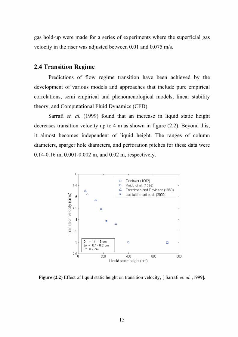
Sarrafi et. al. (1999) found that an increase in liquid static height
decreases transition velocity up to 4 m as shown in figure (2.2). Beyond this,
it almost becomes independent of liquid height. The ranges of column
diameters, sparger hole diameters, and perforation pitches for these data were
0.14-0.16 m, 0.001-0.002 m, and 0.02 m, respectively.
Figure (2.2) Effect of liquid static height on transition velocity, [ Sarrafi et. al. ,1999].
16
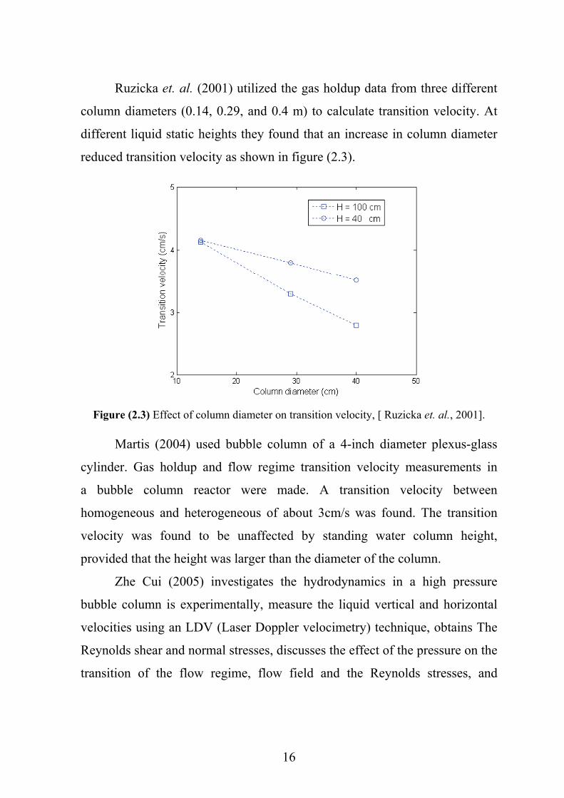
Ruzicka et. al. (2001) utilized the gas holdup data from three different
column diameters (0.14, 0.29, and 0.4 m) to calculate transition velocity. At
different liquid static heights they found that an increase in column diameter
reduced transition velocity as shown in figure (2.3).
Figure (2.3) Effect of column diameter on transition velocity, [ Ruzicka et. al., 2001].
Martis (2004) used bubble column of a 4-inch diameter plexus-glass
cylinder. Gas holdup and flow regime transition velocity measurements in
a bubble column reactor were made. A transition velocity between
homogeneous and heterogeneous of about 3cm/s was found. The transition
velocity was found to be unaffected by standing water column height,
provided that the height was larger than the diameter of the column.
Zhe Cui (2005) investigates the hydrodynamics in a high pressure
bubble column is experimentally, measure the liquid vertical and horizontal
velocities using an LDV (Laser Doppler velocimetry) technique, obtains The
Reynolds shear and normal stresses, discusses the effect of the pressure on the
transition of the flow regime, flow field and the Reynolds stresses, and
17
investigates Furthermore, the effects of the liquid properties on the
hydrodynamics of the bubble column.
Diaz et. al. (2006) used a partially aerated plate and the combined
effect of UG and the liquid height/width of the column ratio (aspect ratio
(H/W) on the resulting flow regimes is studied. The use of partially aerated
plates can generate bubble plumes that show an oscillatory movement and
create ascending and descending liquid circulation structure. The resulting
unsteady flow patterns differ considerably from the time-averaged flow
regimes. The quantitative analysis of the flow regimes is based on the
measurements of wall pressure fluctuations while qualitative description of
the type of flow is obtained by image analysis. The analysis of existing time-
averaged flow patterns for given experimental conditions is based on the
representation of the global gas hold-up (εG) versus U while the study of non-
stationary structures is based on the spectral analysis, a method that provides
information of the oscillation frequency of the bubble plume as well as of the
different physical phenomena taking place in the bubble column through the
resulting spectra and the mean and characteristic frequencies.
18
CHAPTER THREE
THEORITICAL ASPECT
3.1 Hydrodynamic in Bubble Column and Airlift Reactor The hydrodynamics of airlift reactor is strongly affected by liquid
properties as well as by reactor design and operating conditions. A variety of
hydrodynamic regimes establish in the airlift, depending on the choice of
design parameters and tuning of operating conditions [Olivieri et al., 2006].
Gas is dispersed into bubbles using a sparger and bubbles rise through
the liquid. Hence, momentum is transferred from the faster, upward moving
gas phase to the slower liquid phase. Depending on the gas and liquid flow
rates and the physical properties of the system, bubble columns can be
operated in either homogeneous bubbling flow, heterogeneous bubbling flow
or slugging flow regimes. Bubbles play an important role in gas-liquid
system. [Zhe Cui, 2005].
3.2 Factors Influencing Hydrodynamics of Bubble Column
Reactors Factors that influence hydrodynamics of Bubble Column Reactors are
superficial velocity, bubble diameter, column geometry (reactor walls) and
pressure [Urseanu and Krishna, 2000].
These factors are interdependent requiring them to be discussed in
relation to each other rather than independently. Superficial gas velocity can
be defined as volumetric gas flow rate per cross sectional area of bubble
column. Superficial velocity is dependent on column dimensions [Miron et.
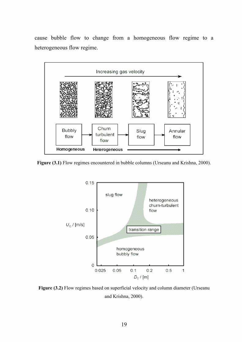
al., 1999]. Figure (3.1) shows that an increase in superficial gas velocity will
19
cause bubble flow to change from a homogeneous flow regime to a
heterogeneous flow regime.
Figure (3.1) Flow regimes encountered in bubble columns (Urseanu and Krishna, 2000).
Figure (3.2) Flow regimes based on superficial velocity and column diameter (Urseanu
and Krishna, 2000).
20
Figure (3.2) shows that the approximate transition from homogeneous
bubble flow to heterogeneous churn-turbulent flow and slug flow is based on
the superficial gas velocity and column diameter [Urseanu and Krishna,
2000]. For a given bubble column, the superficial gas velocity at which
transition occurs would be different for sparged systems because sparged
systems have a fixed number of openings and fixed opening size [Anderson,
2004].
The amount of time the bubble spends in the column is also dependent
up on the height of the bubble column. In a taller bubble column the bubble
has to travel a greater distance allowing more time for mass transfer.
Generally taller bubble columns are preferred over shorter columns to
improve mass transfer efficiency [Anderson, 2004].
Wall effects were found to be negligible in a bubble column with a
single opening and a ratio of bubble diameter to column diameter less than
0.125 [Krishna et. al., 1999].
Bubble diameter and gas holdup can be related by equation (3.1)
(Poulsen and Iversen, 1998; Miron et. al., 2000]. The larger the bubble
diameter, the larger the interfacial surface area is which leads to more mass
transfer due to large gas holdup. A large number of dense small bubbles are
preferred over a small number of large bubbles. The effective interfacial area
of a swarm of small bubbles is greater than for a few large bubbles.
)1(d
6aB
L εε−
= … (3.1)
Pressure affects the flow of bubbles in bubble columns. When external
pressure is applied on the bubble column, bubbles are more homogenous and
the mean bubble velocity is small, increasing gas holdup, and increasing mass
transfer [Anderson, 2004].
21
The pressure effect on the flow regime transition is mainly due to the
change in bubble characteristics, such as bubble size and bubble size
distribution. When bubble column operate at high pressure condition, bubble
coalescence is suppressed and bubble breakup is enhanced. Also, the
distributor tends to generate smaller bubbles. All these factors contribute to
small bubble sizes and narrow bubble size distributions and, consequently,
delay the flow regime transition at high pressures. [Zhe Cui, 2005].
By comparing the pressure effect on the gas holdup with that on the
bubble rise velocity, it can be stated that the increase in gas holdup with
pressure is a consequence of the decreases in both the bubble size and the
bubble rise velocity, i.e. larger bubbles broken into smaller ones and their rise
velocities further reduced by pressure. The decrease in bubble rise velocity
occurs due to corresponding variations of gas and liquid properties with
pressure [Fan et. al., 1998].
Buoyancy force of a bubble is a function of cube of bubble diameter
and drag force is a function of square of bubble diameter (Adkins et. al.,
1996). As the bubble rise from the bottom of the reactor bubble diameter
increases. With the change in diameter of the bubble the buoyancy force and
drag force change, and in turn change the velocity of the bubble. The mean
bubble velocity changes from inception to death or burst at the top of the
column [Anderson, 2004].
3.3 Flow Regime Bubble column flow regimes are broadly classified as homogeneous
and heterogeneous flows (Krishna and Baten, 2003).
22
3.3.1 Homogenous Flow The homogeneous regime is encountered at relatively low gas
velocities and characterized by "small" bubbles, typically in the range of 2 to
6 mm, a narrow bubble size distribution and The rise velocity of these bubbles
does not exceed 0.025 m/s and radially uniform gas holdup and is most
desirable for practical applications, because it offers a large contact area
[Joshi et. al., 2002; Olmos et. al., 2001].
The concentration of bubbles is uniform, particularly in the transverse
direction. The process of coalescence and dispersion are practically absent in
the homogeneous regime and hence the size of bubbles are entirely dictated
by the sparger design and the physical properties of the gas and liquid phases
[Tharat, 1998].
Observed change from bubbly flow to transition flow is asymptotic
depending on various factors [Wallis, 1969] which affect the size of the gas
bubble by altering the degree of coalescence. The flow regime transition is
normally identified based on instability theory, analysis of fluctuation signals,
and the drift flux model. Higher gas density is found to have a stabilizing
effect on the flow and that the gas fraction at the instability point (i.e.,
transition point) increases with gas density, while the gas velocity at the
instability point only slightly increases with gas density. The drift flux of gas
increases with the gas holdup in the dispersed regime; in the coalesced bubble
regime, the rate of increase is much larger [Zhe Cui, 2005].
3.3.2 Heterogeneous Flow Heterogeneous flow is characterized by larger bubbles formed when
small bubbles coalesce and interact with each other and, as a result, the
bubbles have a range of speeds in varied directions. The non-uniform gas
23
holdup distribution across the radial direction causes bulk liquid circulation in
this flow regime [Shaikh and Al-Dahhan, 2007]. Heterogeneous bubble flows
are further classified into churn turbulent flow; slug flow and annular flow as
shown in figure (3.1) [Urseanu and Krishna, 2000].
3.3.2.1 Churn-Turbulent Flows Phenomenologically churn-turbulent flows can be readily described as
follows. At high superficial gas velocities and low liquid superficial velocities
in large diameter vessels high gas holdups are reached (typically well in
excess of 30%) and large spiraling, transient, vortex like structures move
through the column [Hills, 1975, Devanathan, 1991, Chen et al., 1994].
3.3.2.2 Slug Flow This flow is characterized by long “Taylor” bubbles rising and almost
filling a pipe’s cross-section. Liquid moves around the bubbles and fills the
space between two successive gas slugs. While the progress of the gas slugs is
very stable, the area between it is greatly agitated. In industry, slug flow may
appear in nearly any application employing two-phase flow in pipes [Von
Karman, 2006]. This type of flow is characterized by large regions of a lower
density fluid (bubble) surrounded by regions of a higher density fluid (slugs).
From fig. (3.2), it can be inferred that the mean bubble velocity in slug flow
would be high (>0.05 m/s) [Urseanu and Krishna, 2000]. Slug flow regime
transition occurs at constant overall gas holdup [Shaikh and Al-Dahhan,
2007].
24
3.4 Bubble Formation The siz of bubbles generated from gas distributors have a significant
effect on the hydrodynamics and mass transfer in bubbling systems. An
increase gas density was found to reduce the size of bubbles. Discrete bubbles
are formed at low gas velocities. At a high gas velocity, jetting occurs and
bubbles are formed from the top of the jet. In the discrete bubble regime, the
bubble size is relatively uniform; in contrast, the bubbles formed from a jet
are of a wide size distribution [Massimilla et. al., 1961]. The empirical
correlation provided by Idogowa et. al. (1987) indicated that the bubbling-
jetting transition velocity in a liquid is proportional to the gas density to the
power of -0.8. Increasing the air flow increases the frequency of bubble
formation, and, consequently [Nguyena et. al., 1996].
The stability at larger gas fractions is only possible when the bubble
size is small. Larger bubbles cause large-scale turbulence, also at lower gas
fractions. The bubbles experience a horizontal lift force. Its direction depends
on the bubbles’ size and shape – larger bubbles are flatter. Larger bubbles
tend to be drawn to the centre of the column, where they cluster, cause a
lower fluid density, and cause large vortices. The larger bubbles, the sooner a
flow become turbulent. It is therefore necessary to integrate the effect of the
lift force into the computer models [Wouter, 2006].
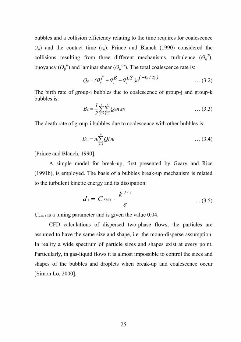
3.5 Bubble Coalescence and Break-up The coalescence of two bubbles is often assumed to occur in three
steps. First the bubbles collide trapping a small amount of liquid between
them. This liquid film then drains until the liquid film separating the bubbles
reaches a critical thickness. The film ruptures and the bubbles join together.
The coalescence process is therefore modeled by a collision rate of two
25
bubbles and a collision efficiency relating to the time requires for coalescence
(tij) and the contact time (τij). Prince and Blanch (1990) considered the
collisions resulting from three different mechanisms, turbulence (ӨijT),
buoyancy (ӨijB) and laminar shear (Өij
LS). The total coalescence rate is:
)/t(e)LSBT(Q ijijijijijij
τθθθ −++= … (3.2)
The birth rate of group-i bubbles due to coalescence of group-j and group-k bubbles is:
∑∑= =
=i
1j
i
1kkjjkC nnQ
21B … (3.3)
The death rate of group-i bubbles due to coalescence with other bubbles is:
∑=
=N
1jjjiC nQinD … (3.4)
[Prince and Blanch, 1990].
A simple model for break-up, first presented by Geary and Rice
(1991b), is employed. The basis of a bubbles break-up mechanism is related
to the turbulent kinetic energy and its dissipation:
ε
2/3
SMDskCd ⋅= ... (3.5)
CSMD is a tuning parameter and is given the value 0.04.
CFD calculations of dispersed two-phase flows, the particles are
assumed to have the same size and shape, i.e. the mono-disperse assumption.
In reality a wide spectrum of particle sizes and shapes exist at every point.
Particularly, in gas-liquid flows it is almost impossible to control the sizes and
shapes of the bubbles and droplets when break-up and coalescence occur
[Simon Lo, 2000].
26
3.6 Bubbles Motion In airlift reactors larger bubbles rise with liquid in the riser section. On
the other hand, smaller bubbles are carried downward by liquid circulation in
both the riser and down-comer sections. However, the actual amount of air
that circulates through the down-comer is quite small [Kumar, 2006].
As the characteristics of bubble motion and bubble interfacial dynamics
govern the performance of the bubbling systems, the understanding and hence
the ability of controlling the bubble motion and interfacial dynamics are
important to effective operation of these systems.
However, in the reality, rising bubbles with a diameter larger than 5 mm are
always not spherical. Bubbles oscillate with a certain frequency during the
rising period [Zhe Cui, 2005].
In the churn turbulent regime the "large" bubbles (dB > 0.015 m)
formed by coalescence of small bubbles are rising much faster, typically in
the range of 1-2 m/s. They "churn" up the liquid phase and cause an intense
mixing in the column. As an opposite phenomenon to the coalescence, the
large bubbles are breaking up. Therefore the "dynamics" of large bubbles is
continuously determined by buble-buble interaction, characterized by high
frequency coalescence and breaking up.
3.7 Relationship between the riser and down comer gas holdup
in airlift reactors:- The volumetric flow rate of liquid in the riser of an airlift reactor can be
expressed in terms of the superficial liquid velocity in the riser and it's cross
sectional area; thus,
rLrLr AUQ = … (3.6)
27
where QLr is the liquid flow rate, ULr is the superficial liquid velocity in the
riser, and Ar is the riser cross-sectional area. Similarly, for the down comer we
have
dLdLd AUQ = … (3.7)
where ULd is the superficial liquid velocity in the down comer and Ad is the
down comer cross-sectional area. Because all the liquid exiting the down
comer circulates through the riser, i.e., QLr = QLd, from eqs (3.6) and (3.7), we
have
dLdrLr AUAU = … (3.8)
Equation (3.8) can be written in terms of the linear liquid velocities in the
various zones:
)1(AV)1(AV ddLdrrLr εε −=− … (3.9)
Where V Lr and VLd are the linear liquid velocities in the riser and down comer,
respectively, and εr and εd are the respective gas-holdups.
Rearrange of equation (3.9) leads to
⎟⎠⎞
⎜⎝⎛ −−= 1
AVAV
AVAV
dLd
rLrr
rLd
rLrd εε … (3.10)
Equation (3.10) is an explicit relationship between the riser and down comer
holdups. The equation is quite general and it applies ton any airlift reactor,
irrespective of the liquid and the gas phases used. Equation (3.10) may be
written as
βαεε −= rd … (3.11)
where
28
dLd
rLr
AVAV
=α … (3.12)
and
1−=αβ … (3.13)
Equation (3.11) has the same form as many empirical correlations found in
table (3.1). Frequently, β has been neglected as being negligibly small, and
equ. (3.11) has been simplified to
rd αεε = … (3.14)
A multitude of correlations such as equations (3.11) and (3.14) are available
as summarized in table (3.1); how ever, most of those equations differ on the
values of the parameters α and β.
The parameters α and β supposedly depend on the geometry of the
reactor (internal or external loop), the liquid and gas phases used, and the
regime of the operation. The α-values have normally ranged over 0.8-0.9
(Chisti, 1989). Lower value of α have been reported, but values equaling unity
or higher have never been observed.
Note that a constant value of α in a given reactor implies that the ratio
VLr/VLd is not sensitive to the gas flow rate or the gas holdup in the riser. This
appears to be the case over much of the operational range for internal loop
type of airlift reactors without especial gas-liquid separators. However, a
constant VLr /VLd can not be assumed generally; hence, in some cases the
linear equation (3.11) could break down. This would happen mostly in airlift
devices with gas-liquid separators. With an effective gas-liquid separator, the
down comer gas holdup will be nil, and equation (3.11) will be take the form
α
ε 11r −= … (3.15)
29
Because the riser gas holdup must increase with increasing gas flow rate, the
α-value must increase. In a reactor with no gas in the down comer, the bounds
of variation of α can be shown to be 0 ≤ 1/ α ≤ 1.
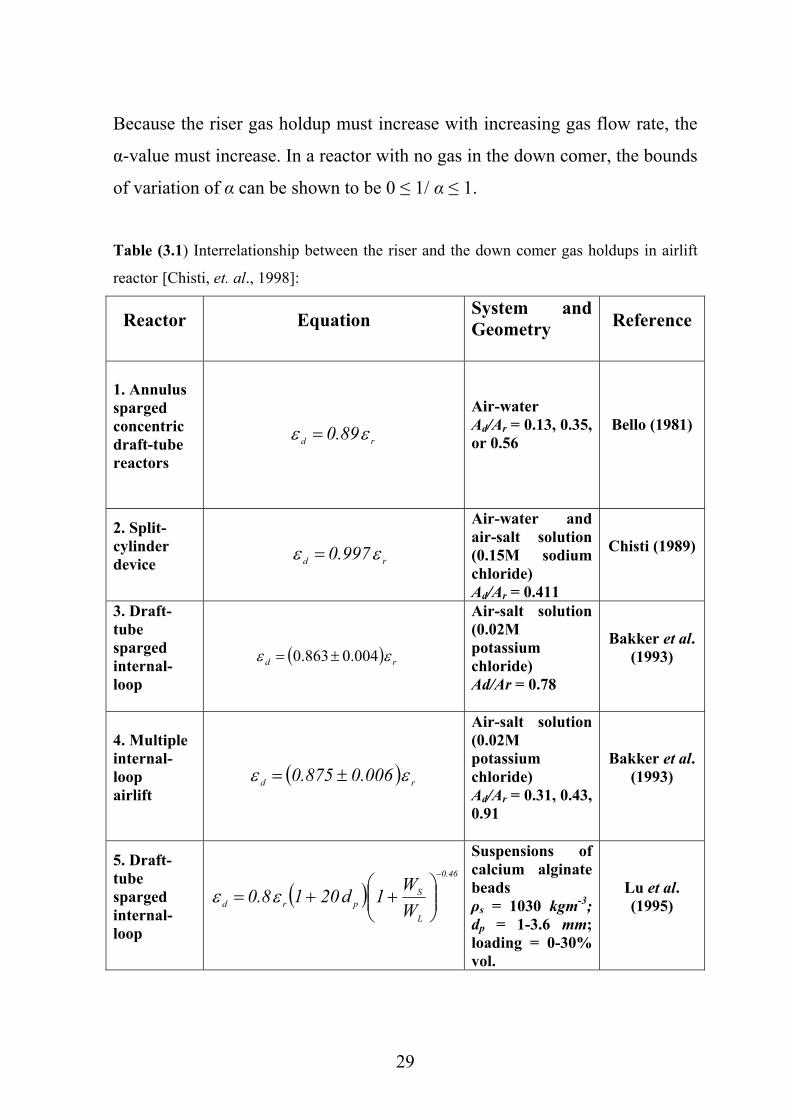
Table (3.1) Interrelationship between the riser and the down comer gas holdups in airlift
reactor [Chisti, et. al., 1998]:
Reactor
Equation
System and Geometry
Reference
1. Annulus sparged concentric draft-tube reactors
rd 89.0 εε =
Air-water Ad/Ar = 0.13, 0.35, or 0.56
Bello (1981)
2. Split-cylinder device
rd 997.0 εε =
Air-water and air-salt solution (0.15M sodium chloride) Ad/Ar = 0.411
Chisti (1989)
3. Draft-tube sparged internal-loop
( ) rd εε 004.0863.0 ±=
Air-salt solution (0.02M potassium chloride) Ad/Ar = 0.78
Bakker et al. (1993)
4. Multiple internal-loop airlift
( ) rd 006.0875.0 εε ±=
Air-salt solution (0.02M potassium chloride) Ad/Ar = 0.31, 0.43, 0.91
Bakker et al. (1993)
5. Draft-tube sparged internal-loop
( )46.0
L
Sprd W
W1d2018.0−
⎟⎟⎠
⎞⎜⎜⎝
⎛++= εε
Suspensions of calcium alginate beads ρs = 1030 kgm-3; dp = 1-3.6 mm; loading = 0-30% vol.
Lu et al. (1995)
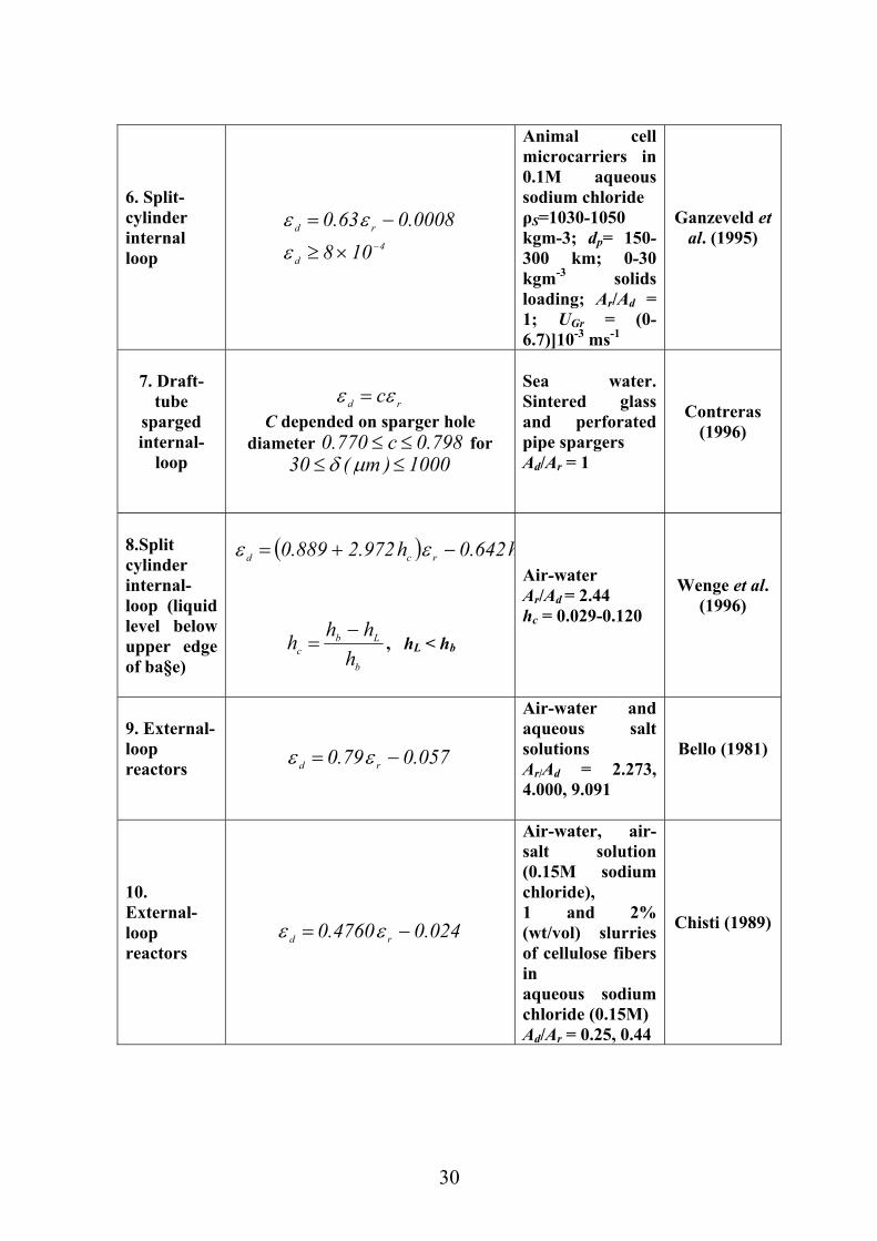
30
6. Split-cylinder internal loop
4d
rd
1080008.063.0
−×≥
−=
εεε
Animal cell microcarriers in 0.1M aqueous sodium chloride ρS=1030-1050 kgm-3; dp= 150-300 km; 0-30 kgm-3 solids loading; Ar/Ad = 1; UGr = (0-6.7)]10-3 ms-1
Ganzeveld et al. (1995)
7. Draft-
tube sparged internal-
loop
rd cεε = C depended on sparger hole
diameter 798.0c770.0 ≤≤ for 1000)m(30 ≤≤ µδ
Sea water. Sintered glass and perforated pipe spargers Ad/Ar = 1
Contreras (1996)
8.Split cylinder internal-loop (liquid level below upper edge of ba§e)
( ) rcd h642.0h972.2889.0 −+= εε
b
Lbc h
hhh −= , hL < hb
Air-water Ar/Ad = 2.44 hc = 0.029-0.120
Wenge et al. (1996)
9. External-loop reactors
057.079.0 rd −= εε
Air-water and aqueous salt solutions Ar/Ad = 2.273, 4.000, 9.091
Bello (1981)
10. External-loop reactors
024.04760.0 rd −= εε
Air-water, air-salt solution (0.15M sodium chloride), 1 and 2% (wt/vol) slurries of cellulose fibers in aqueous sodium chloride (0.15M) Ad/Ar = 0.25, 0.44
Chisti (1989)
31
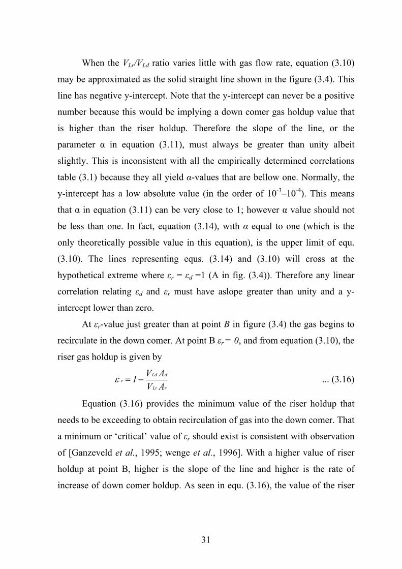
When the VLr/VLd ratio varies little with gas flow rate, equation (3.10)
may be approximated as the solid straight line shown in the figure (3.4). This
line has negative y-intercept. Note that the y-intercept can never be a positive
number because this would be implying a down comer gas holdup value that
is higher than the riser holdup. Therefore the slope of the line, or the
parameter α in equation (3.11), must always be greater than unity albeit
slightly. This is inconsistent with all the empirically determined correlations
table (3.1) because they all yield α-values that are bellow one. Normally, the
y-intercept has a low absolute value (in the order of 10-3–10-4). This means
that α in equation (3.11) can be very close to 1; however α value should not
be less than one. In fact, equation (3.14), with α equal to one (which is the
only theoretically possible value in this equation), is the upper limit of equ.
(3.10). The lines representing equs. (3.14) and (3.10) will cross at the
hypothetical extreme where εr = εd =1 (A in fig. (3.4)). Therefore any linear
correlation relating εd and εr must have aslope greater than unity and a y-
intercept lower than zero.
At εr-value just greater than at point B in figure (3.4) the gas begins to
recirculate in the down comer. At point B εr = 0, and from equation (3.10), the
riser gas holdup is given by
rLr
dLdr
AVAV1−=ε ... (3.16)
Equation (3.16) provides the minimum value of the riser holdup that
needs to be exceeding to obtain recirculation of gas into the down comer. That
a minimum or ‘critical’ value of εr should exist is consistent with observation
of [Ganzeveld et al., 1995; wenge et al., 1996]. With a higher value of riser
holdup at point B, higher is the slope of the line and higher is the rate of
increase of down comer holdup. As seen in equ. (3.16), the value of the riser
32
holdup needed to obtain recirculation of gas in the down comer depends on
the liquid velocity in the down comer and the riser.
Figure (3.3) Schematic representation of equation (3.10).
3.8 Axial liquid velocity The development of liquid velocity profiles along the axial direction is
examined by the measurements of liquid velocity profiles at different axial
positions above the distributor [Zhe Cui, 2005].
Average liquid velocity was related to superficial liquid velocity by [Taitel et
al., 1980]:
G
LL 1
UVε−
= … (3.13)
Liquid circulation velocity distinguishes airlift from bubble column
contactors where the average liquid velocity is zero. Liquid velocity in the
airlift contactor was determined as a function of the superficial gas velocity,
vG, using the flow-follower method [Mercer, 1981].
Maximum centerline axial liquid velocity depending on reactor diameter,
superficial gas velocity, liquid viscosity and density [Riquarts,1981] and
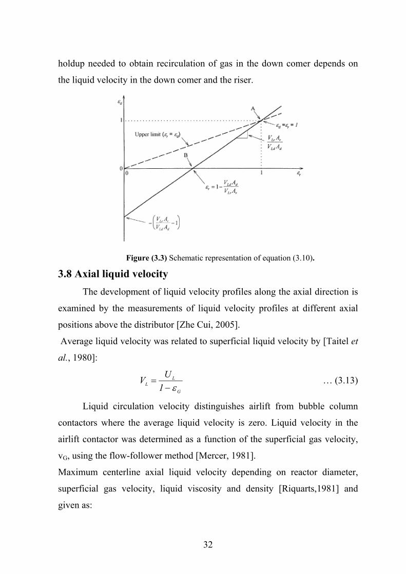
given as:
33
8/1
l
t3
0,Gmax,ax,l g
UgD21.0V ⎟⎟
⎠
⎞⎜⎜⎝
⎛⋅⋅
⋅⋅=µ
ρ ... (3.14)
Correlations for the prediction of radial profiles of axial liquid velocity have
been presented by [Kawase and Moo-Young, 1986] have presented a rather
simple correlation for radial profiles of axial liquid flow velocity in two-phase
bubble columns:
1Rr2
VV 2
max,ax,L
L +⎟⎠⎞
⎜⎝⎛−= …(3.14a)
This equation corresponds to a parabolic velocity profile where the maximum
down flow velocity at the reactor edge equals the maximum up flow velocity
in the reactor center.
The following form was considered for gas holdup radial distribution:
⎥⎦⎤
⎢⎣⎡ −⎥⎦⎤
⎢⎣⎡ +
= nGG )
Rr(1
n2nεε … (3.15)
Where n = 2 for an air-water system [Kelkar 1986]. 3.9 Transition Regime An increase in superficial gas velocity increases the centerline liquid
axial velocity up to a maximum value, concluded that the maximum indicates
the transition from homogeneous to heterogeneous flow. Because no gas
holdup data was provided, it is not known whether the maximum in centerline
axial velocity is due to the S-shaped gas holdup curve that might be present in
their system [Franz et. al., 1984].
However, when the change in slope is gradual or the gas holdup curve
does not show a maximum in gas holdup, it is difficult to identify the
transition point. In such cases, the drift flux method proposed by Wallis,
(1969) has been used extensively.
34
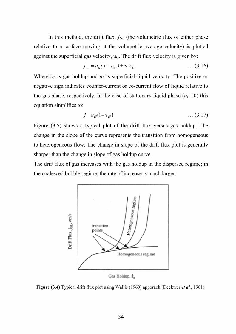
In this method, the drift flux, jGL (the volumetric flux of either phase
relative to a surface moving at the volumetric average velocity) is plotted
against the superficial gas velocity, uG. The drift flux velocity is given by:
GLGGGL u)1(uj εε ±−= … (3.16)
Where εG is gas holdup and uL is superficial liquid velocity. The positive or
negative sign indicates counter-current or co-current flow of liquid relative to
the gas phase, respectively. In the case of stationary liquid phase (uL= 0) this
equation simplifies to:
( )GGuj ε−= 1 … (3.17)
Figure (3.5) shows a typical plot of the drift flux versus gas holdup. The
change in the slope of the curve represents the transition from homogeneous
to heterogeneous flow. The change in slope of the drift flux plot is generally
sharper than the change in slope of gas holdup curve.
The drift flux of gas increases with the gas holdup in the dispersed regime; in
the coalesced bubble regime, the rate of increase is much larger.
Figure (3.4) Typical drift flux plot using Wallis (1969) apporach (Deckwer et al., 1981).
35
The transition velocity depends on a number of factors such as gas
distributor design, physical properties of the phases, and column size. The
transition velocity is higher at higher system pressures and/or temperatures
[Zhe Cui, 2005].
The following equations to predict transition velocity and holdup:
)193exp(5.0UU 11.05.0
L61.0
Gtranb,s
tran σµρε −−== … (3.18)
03.0
G
L273.04L
L3
Lb,s ][]g
[23.2U
ρρ
µρσ
σµ −= … (3.19)
Where Us,b is the rise velocity of the bubbles [Wilkinson et al., 1992].
36
CHAPTER FOUR
RESULTS AND DISCUSSION
4.1 Computational Fluid Dynamics (CFD) Simulations All the mentioned factors in chapter three which influence
hydrodynamics of airlift reactors and bubble column greatly influence the
liquid recurrent in the column. The simulations are the best way to study the
gas holdup and liquid velocity in airlift reactors and bubble column because
experimentation consuming time, costly, and it is difficult to separate effects
of interdependent variables by testing. CFD simulations will allow variable
affects to be studied and optimized before a system is designed and tested
[Anderson, 2004].
4.2 Computing Technology Rapid progress in three influencing technologies over the past two
decades has brought CFD to the forefront of process engineering. Advances in
computational technology, and sustained effort by CFD providers to
implement comprehensive physical models, and advances in numerical
methods have combined to make it possible for engineering to use CFD
routinely in many process industrial companies [Haidari and Matthews,
2003].
ANSYS Inc., found in (1970) develops and globally markets
engineering simulation software and technologies widely used by engineers
and designers across abroad spectrum of industries. The company focuses on
the development of open and flexible solutions that enable users to analyze
design directly on the desktop, providing a common plate form for fast,
37
efficient and cost-conscious product development, from design concept to
final-stage testing and validation.
CFX-5 includes a variety of multiphase models to allow the simulation
of processes which transport and bring into direct contact multiple fluid
streams to effect mixing, reaction, and separation. Multiphase flow in CFX-5
useing Eulerian–Eulerian multiphase model. Two different sub-models are
available for Eulerian-Eulerian multiphase flow:
• The Homogeneous Model: This is the simplest model, in which all
fluids share the same flow field.
• The Inter-fluid Transfer or Inhomogeneous Model: Each fluid
possesses its own flow field and the fluids interact via interphase
transfer terms. Two different sub-models are available which differ in
the way they model the interphase transfer terms. These are: the
Particle Model and the Mixture Model [Wang et. al., 2003].
4.3 Development of CFD Model In present work Eulerian simulations were carried out for an airlift
reactor using 3-D CFX-5, shown schematically in figure (4.1). This geometry
corresponds to an experimental setup used by Baten et. al., (1999) Consisting
of a polyacrylate column with an inner diameter of 0.15 m and a length of 2
m. At the bottom of the column, the gas phase is introduced through a
perforated plate with 108 holes of 0.5 mm in diameter. A polyacrylate draft
tube (riser) of 0.10 m inner and 0.11 m outer diameter, with a length of 2.02
m, is mounted into the column 0.10 m above the gas distributor. A gas-liquid
separator is mounted at the top of the column of 1 m in height and 0.38m in
diameter. The main purposes of the separator of airlift reactors, where the
riser and the downcomer interconnect, are the gas disengagement and avoid
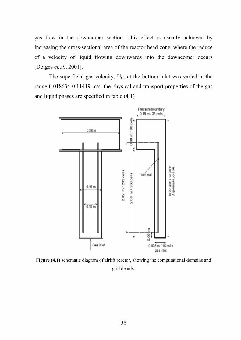
38
gas flow in the downcomer section. This effect is usually achieved by
increasing the cross-sectional area of the reactor head zone, where the reduce
of a velocity of liquid flowing downwards into the downcomer occurs
[Dolgos et.al., 2001].
The superficial gas velocity, UG, at the bottom inlet was varied in the
range 0.018634-0.11419 m/s. the physical and transport properties of the gas
and liquid phases are specified in table (4.1)
Figure (4.1) schematic diagram of airlift reactor, showing the computational domains and
grid details.
39
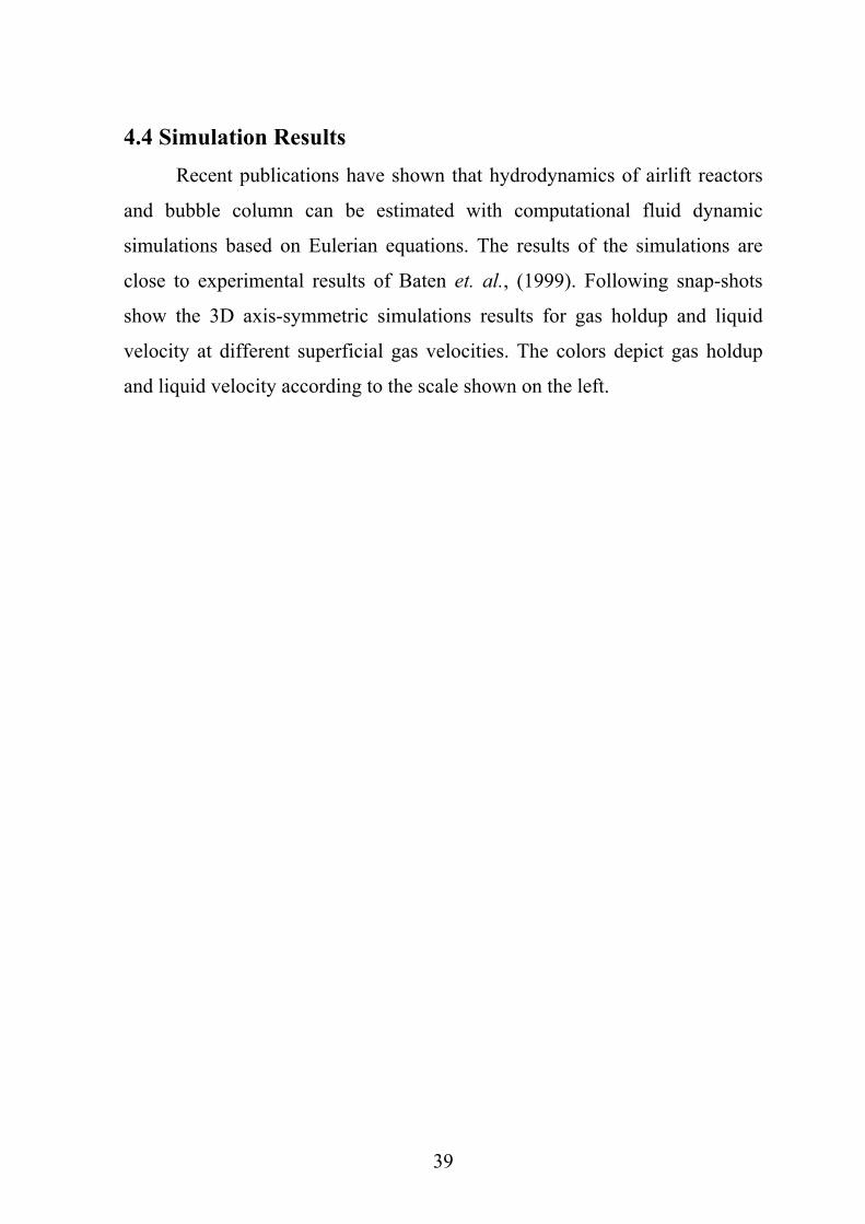
4.4 Simulation Results Recent publications have shown that hydrodynamics of airlift reactors
and bubble column can be estimated with computational fluid dynamic
simulations based on Eulerian equations. The results of the simulations are
close to experimental results of Baten et. al., (1999). Following snap-shots
show the 3D axis-symmetric simulations results for gas holdup and liquid
velocity at different superficial gas velocities. The colors depict gas holdup
and liquid velocity according to the scale shown on the left.
40
Figure (4.2) Contours of air volume fraction and liquid velocity at 0.018634 m/s
superficial gas velocity.
Table (4.1) Local and average gas holdup and liquid velocity in riser and downcomer at
0.018634 m/s superficial gas velocity.
Z (m) εr (-) VLr (m/s) VLd (m/s) 0.1 0.0372094 0.657394 0.35544 1 0.01781 0.394913 0.363036 2 0.0178034 0.396347 0.286648
avg. 0.024274 0.482885 0.33501133
41
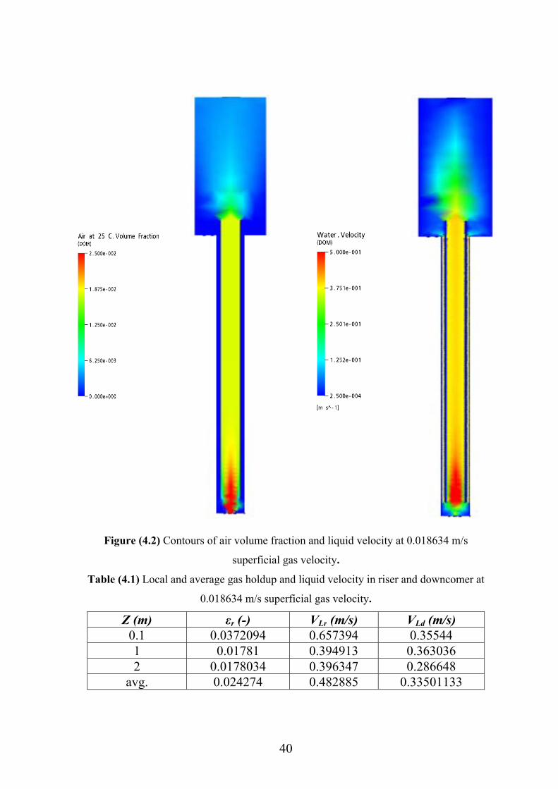
Figure (4.3) Contours of air volume fraction and liquid velocity at 0.040887m/s superficial
gas velocity.
Table (4.2) Local and average gas holdup and liquid velocity in riser and downcomer at
0.040887m/s superficial gas velocity.
Z (m) εr (-) VLr (m/s) VLd (m/s) 0.1 0.0884672 0.616815 0.47503 1 0.0295163 0.520283 0.503896 2 0.0295413 0.521975 0.541629
avg. 0.049175 0.553024 0.50685167
42
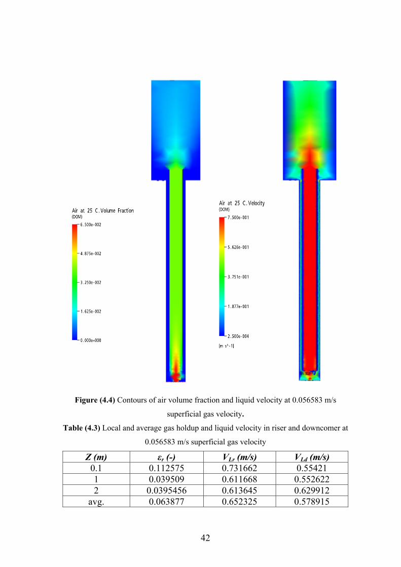
Figure (4.4) Contours of air volume fraction and liquid velocity at 0.056583 m/s
superficial gas velocity.
Table (4.3) Local and average gas holdup and liquid velocity in riser and downcomer at
0.056583 m/s superficial gas velocity
Z (m) εr (-) VLr (m/s) VLd (m/s) 0.1 0.112575 0.731662 0.55421 1 0.039509 0.611668 0.552622 2 0.0395456 0.613645 0.629912
avg. 0.063877 0.652325 0.578915
43
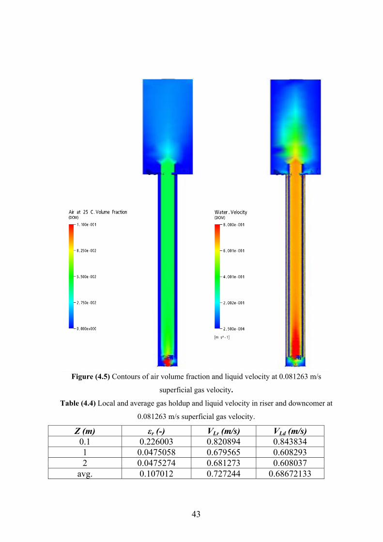
Figure (4.5) Contours of air volume fraction and liquid velocity at 0.081263 m/s
superficial gas velocity.
Table (4.4) Local and average gas holdup and liquid velocity in riser and downcomer at
0.081263 m/s superficial gas velocity.
Z (m) εr (-) VLr (m/s) VLd (m/s) 0.1 0.226003 0.820894 0.843834 1 0.0475058 0.679565 0.608293 2 0.0475274 0.681273 0.608037
avg. 0.107012 0.727244 0.68672133
44
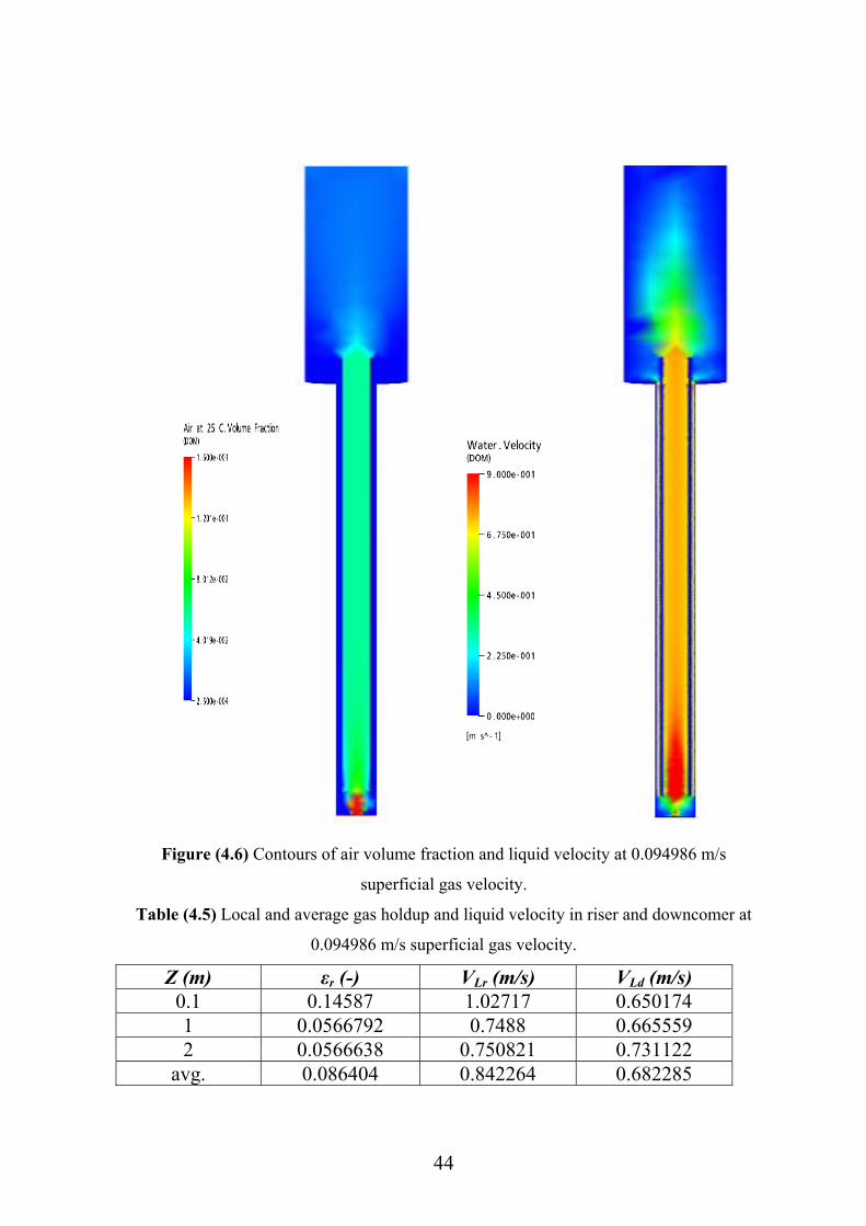
Figure (4.6) Contours of air volume fraction and liquid velocity at 0.094986 m/s
superficial gas velocity.
Table (4.5) Local and average gas holdup and liquid velocity in riser and downcomer at
0.094986 m/s superficial gas velocity.
Z (m) εr (-) VLr (m/s) VLd (m/s) 0.1 0.14587 1.02717 0.650174 1 0.0566792 0.7488 0.665559 2 0.0566638 0.750821 0.731122
avg. 0.086404 0.842264 0.682285
45
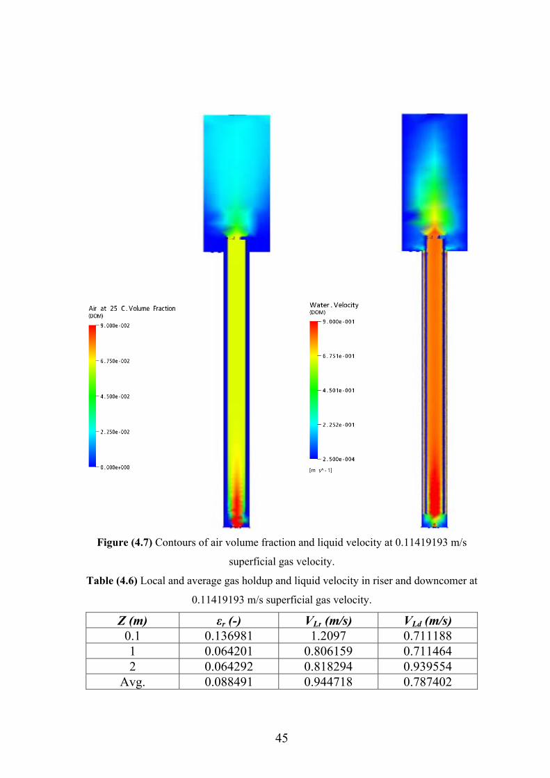
Figure (4.7) Contours of air volume fraction and liquid velocity at 0.11419193 m/s
superficial gas velocity.
Table (4.6) Local and average gas holdup and liquid velocity in riser and downcomer at
0.11419193 m/s superficial gas velocity.
Z (m) εr (-) VLr (m/s) VLd (m/s) 0.1 0.136981 1.2097 0.711188 1 0.064201 0.806159 0.711464 2 0.064292 0.818294 0.939554
Avg. 0.088491 0.944718 0.787402
46
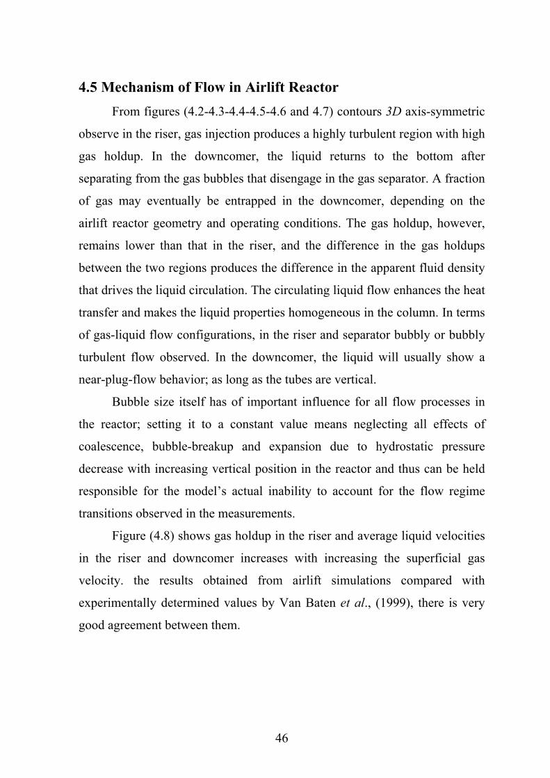
4.5 Mechanism of Flow in Airlift Reactor From figures (4.2-4.3-4.4-4.5-4.6 and 4.7) contours 3D axis-symmetric
observe in the riser, gas injection produces a highly turbulent region with high
gas holdup. In the downcomer, the liquid returns to the bottom after
separating from the gas bubbles that disengage in the gas separator. A fraction
of gas may eventually be entrapped in the downcomer, depending on the
airlift reactor geometry and operating conditions. The gas holdup, however,
remains lower than that in the riser, and the difference in the gas holdups
between the two regions produces the difference in the apparent fluid density
that drives the liquid circulation. The circulating liquid flow enhances the heat
transfer and makes the liquid properties homogeneous in the column. In terms
of gas-liquid flow configurations, in the riser and separator bubbly or bubbly
turbulent flow observed. In the downcomer, the liquid will usually show a
near-plug-flow behavior; as long as the tubes are vertical.
Bubble size itself has of important influence for all flow processes in
the reactor; setting it to a constant value means neglecting all effects of
coalescence, bubble-breakup and expansion due to hydrostatic pressure
decrease with increasing vertical position in the reactor and thus can be held
responsible for the model’s actual inability to account for the flow regime
transitions observed in the measurements.
Figure (4.8) shows gas holdup in the riser and average liquid velocities
in the riser and downcomer increases with increasing the superficial gas
velocity. the results obtained from airlift simulations compared with
experimentally determined values by Van Baten et al., (1999), there is very
good agreement between them.
47
0
0.01
0.02
0.03
0.04
0.05
0.06
0.07
0.08
0.09
0.1
0 0.02 0.04 0.06 0.08 0.1 0.12 0.14
Superficial gas velocity, [m/s]
Gas
hol
dup
in ri
ser,
[-]
EXP.SIM.
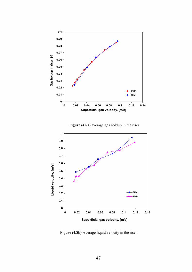
Figure (4.8a) average gas holdup in the riser
0
0.1
0.2
0.3
0.4
0.5
0.6
0.7
0.8
0.9
1
0 0.02 0.04 0.06 0.08 0.1 0.12 0.14
Superficial gas velocity, [m/s]
Liqu
id v
eloc
ity, [
m/s
]
SIM.EXP.
Figure (4.8b) Average liquid velocity in the riser
48
0
0.2
0.4
0.6
0.8
1
1.2
0 0.02 0.04 0.06 0.08 0.1 0.12 0.14
Superficial gas velocity,[m/s]
Liqu
id v
eloc
ity,[m
/s]
EXP.SIM.
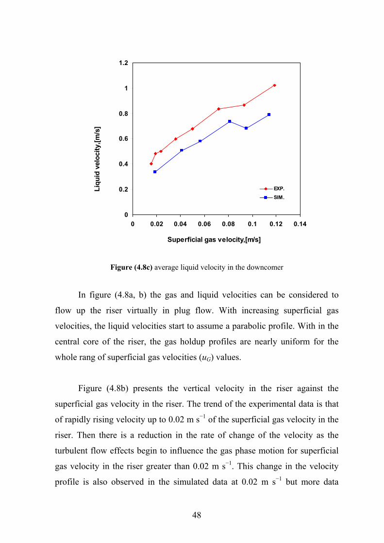
Figure (4.8c) average liquid velocity in the downcomer
In figure (4.8a, b) the gas and liquid velocities can be considered to
flow up the riser virtually in plug flow. With increasing superficial gas
velocities, the liquid velocities start to assume a parabolic profile. With in the
central core of the riser, the gas holdup profiles are nearly uniform for the
whole rang of superficial gas velocities (uG) values.
Figure (4.8b) presents the vertical velocity in the riser against the
superficial gas velocity in the riser. The trend of the experimental data is that
of rapidly rising velocity up to 0.02 m s−1 of the superficial gas velocity in the
riser. Then there is a reduction in the rate of change of the velocity as the
turbulent flow effects begin to influence the gas phase motion for superficial
gas velocity in the riser greater than 0.02 m s−1. This change in the velocity
profile is also observed in the simulated data at 0.02 m s−1 but more data
49
points are required below this value to confirm the change. But generally the
profile of the simulated data fits the empirical profile.
Figure (4.8c) presents the liquid phase velocity in the downcomer. The
flow regime changes as the influence of turbulent flow effects increase. The
simulated data consistently over-predicts the liquid velocity and though the
profile is not linear, more data is required for the lower range of superficial
gas velocities is required to confirm this effect. Because of the presence of
separator, the gas holdup in downcomer approximately broke. Therefore the
reduction appears in the accuracy of the flow data of simulation between the
riser and downcomer. and also There are three effects in the model used that
could influence the accuracy of the simulation in the downcomer, the use of a
single gas fraction of a mean bubble size, the volume fraction equation
formulation and the resolution of the mesh in the downcomer.
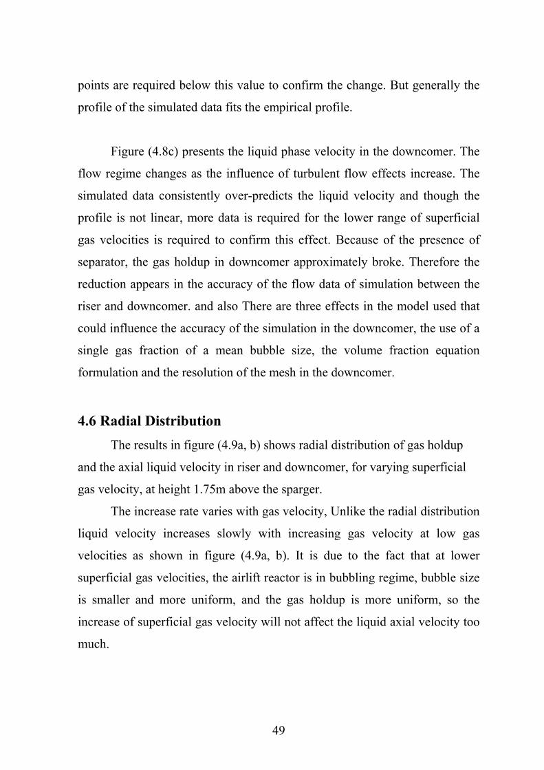
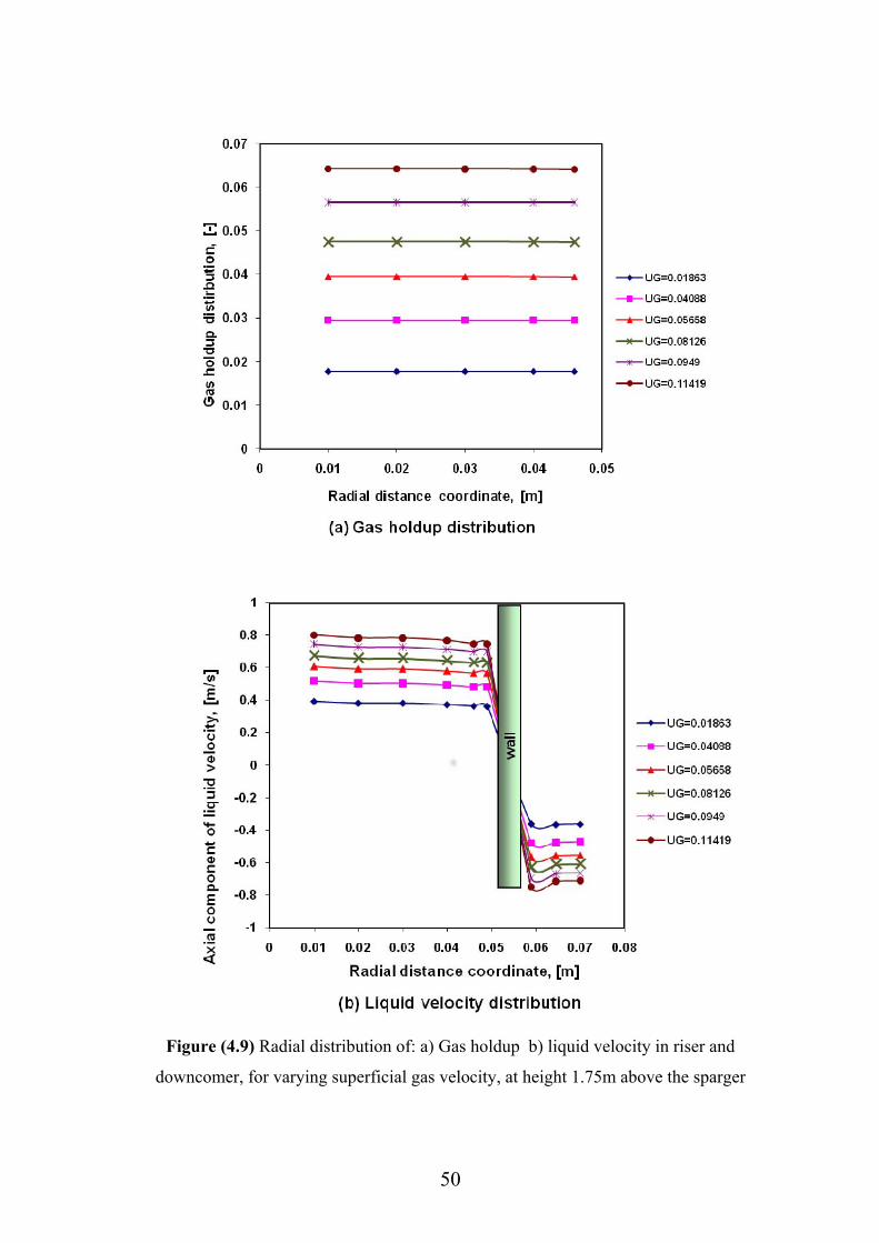
4.6 Radial Distribution The results in figure (4.9a, b) shows radial distribution of gas holdup
and the axial liquid velocity in riser and downcomer, for varying superficial
gas velocity, at height 1.75m above the sparger.
The increase rate varies with gas velocity, Unlike the radial distribution
liquid velocity increases slowly with increasing gas velocity at low gas
velocities as shown in figure (4.9a, b). It is due to the fact that at lower
superficial gas velocities, the airlift reactor is in bubbling regime, bubble size
is smaller and more uniform, and the gas holdup is more uniform, so the
increase of superficial gas velocity will not affect the liquid axial velocity too
much.
50
Figure (4.9) Radial distribution of: a) Gas holdup b) liquid velocity in riser and
downcomer, for varying superficial gas velocity, at height 1.75m above the sparger
51
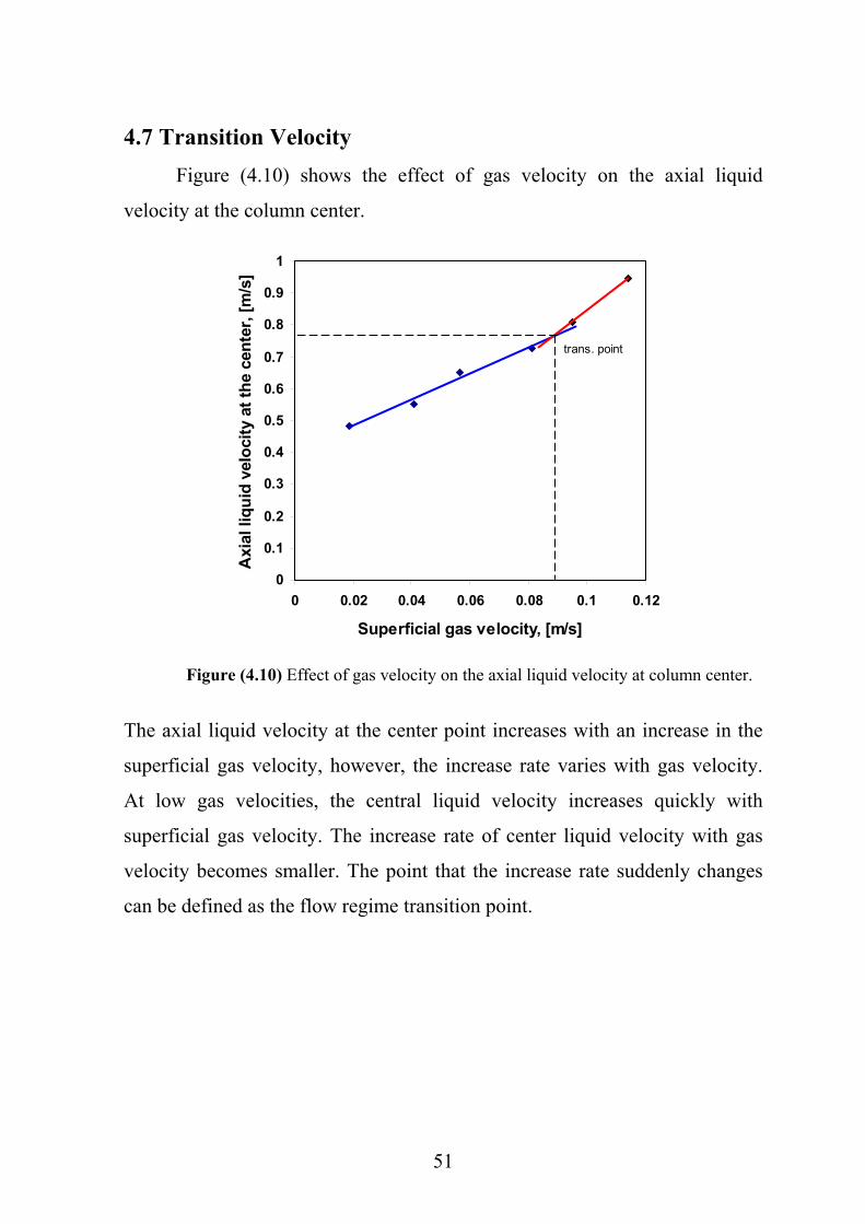
4.7 Transition Velocity Figure (4.10) shows the effect of gas velocity on the axial liquid
velocity at the column center.
0
0.1
0.2
0.3
0.4
0.5
0.6
0.7
0.8
0.9
1
0 0.02 0.04 0.06 0.08 0.1 0.12
Superficial gas velocity, [m/s]
Axi
al li
quid
vel
ocity
at t
he c
ente
r, [m
/s]
trans. point
Figure (4.10) Effect of gas velocity on the axial liquid velocity at column center.
The axial liquid velocity at the center point increases with an increase in the
superficial gas velocity, however, the increase rate varies with gas velocity.
At low gas velocities, the central liquid velocity increases quickly with
superficial gas velocity. The increase rate of center liquid velocity with gas
velocity becomes smaller. The point that the increase rate suddenly changes
can be defined as the flow regime transition point.
52
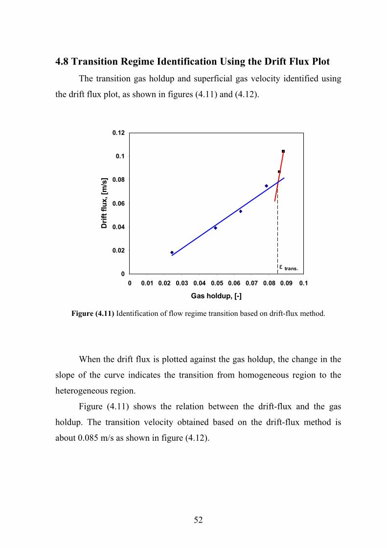
4.8 Transition Regime Identification Using the Drift Flux Plot The transition gas holdup and superficial gas velocity identified using
the drift flux plot, as shown in figures (4.11) and (4.12).
0
0.02
0.04
0.06
0.08
0.1
0.12
0 0.01 0.02 0.03 0.04 0.05 0.06 0.07 0.08 0.09 0.1
Gas holdup, [-]
Drif
t flu
x, [m
/s]
ε trans.
Figure (4.11) Identification of flow regime transition based on drift-flux method.
When the drift flux is plotted against the gas holdup, the change in the
slope of the curve indicates the transition from homogeneous region to the
heterogeneous region.
Figure (4.11) shows the relation between the drift-flux and the gas
holdup. The transition velocity obtained based on the drift-flux method is
about 0.085 m/s as shown in figure (4.12).
53
0
0.01
0.02
0.03
0.04
0.05
0.06
0.07
0.08
0.09
0.1
0 0.02 0.04 0.06 0.08 0.1 0.12
Superficial gas velocity, [m/s]
Gas
hol
dup
in ri
ser,
[-] εGtrans
uGtrans
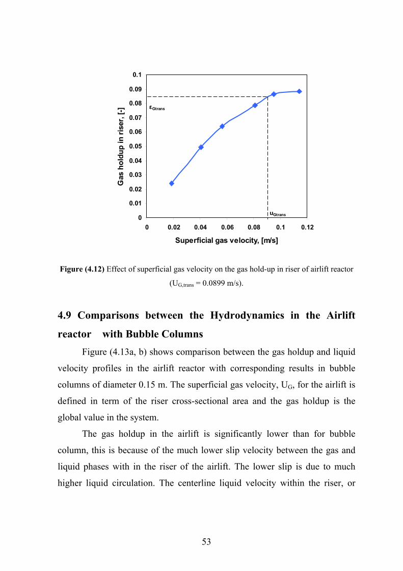
Figure (4.12) Effect of superficial gas velocity on the gas hold-up in riser of airlift reactor
(UG,trans = 0.0899 m/s).
4.9 Comparisons between the Hydrodynamics in the Airlift
reactor with Bubble Columns Figure (4.13a, b) shows comparison between the gas holdup and liquid
velocity profiles in the airlift reactor with corresponding results in bubble
columns of diameter 0.15 m. The superficial gas velocity, UG, for the airlift is
defined in term of the riser cross-sectional area and the gas holdup is the
global value in the system.
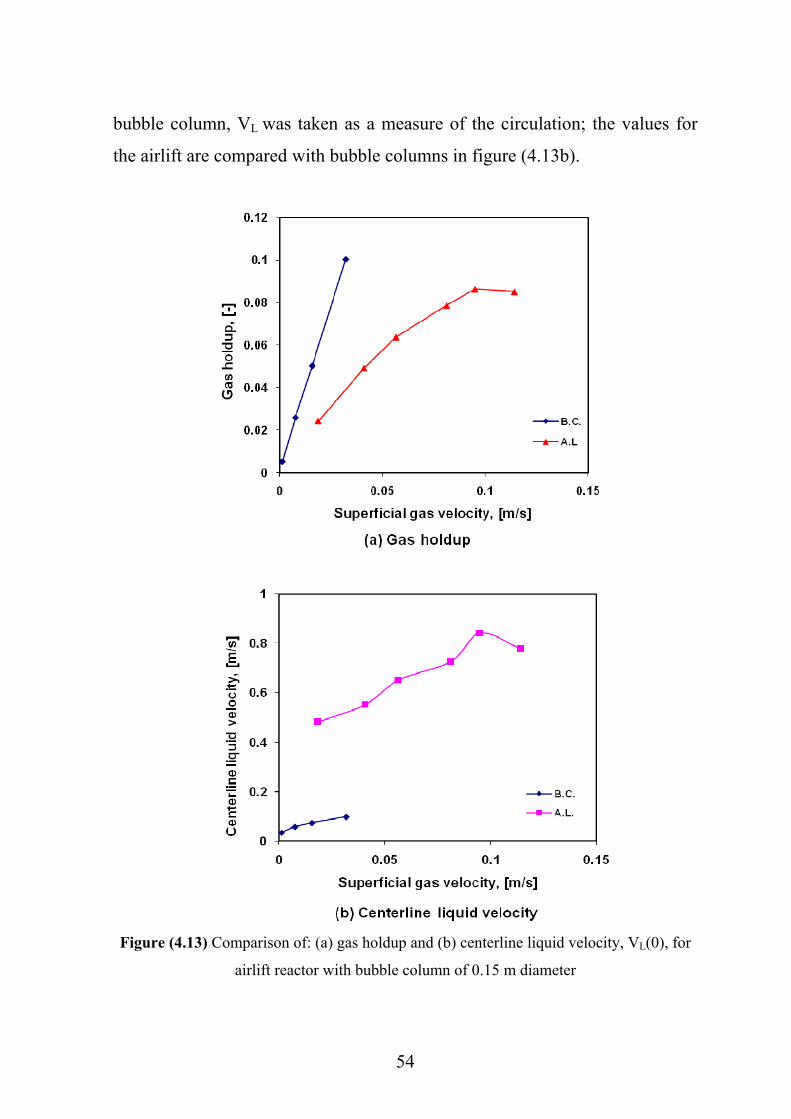
The gas holdup in the airlift is significantly lower than for bubble
column, this is because of the much lower slip velocity between the gas and
liquid phases with in the riser of the airlift. The lower slip is due to much
higher liquid circulation. The centerline liquid velocity within the riser, or
54
bubble column, VL was taken as a measure of the circulation; the values for
the airlift are compared with bubble columns in figure (4.13b).
Figure (4.13) Comparison of: (a) gas holdup and (b) centerline liquid velocity, VL(0), for
airlift reactor with bubble column of 0.15 m diameter
55
The bubble column simulation results presented in figure (4.13) are
restricted to UG values below 0.04m/s because for higher value of UG the
heterogeneous or churn-turbulent regime of operation is entered into [Baten
and Krishna, 2002] as shown in figures (4.14) and (4.15) .
The airlift reactor can be operated at UG values up to 0.12 m/s while
maintaining the homogenous bubble flow regime since the effective slip
velocity in the riser is much lower. The ability to operate in the homogeneous
bubble flow regime till much higher superficial gas velocities than bubble
column is major advantage of the airlift reactors.
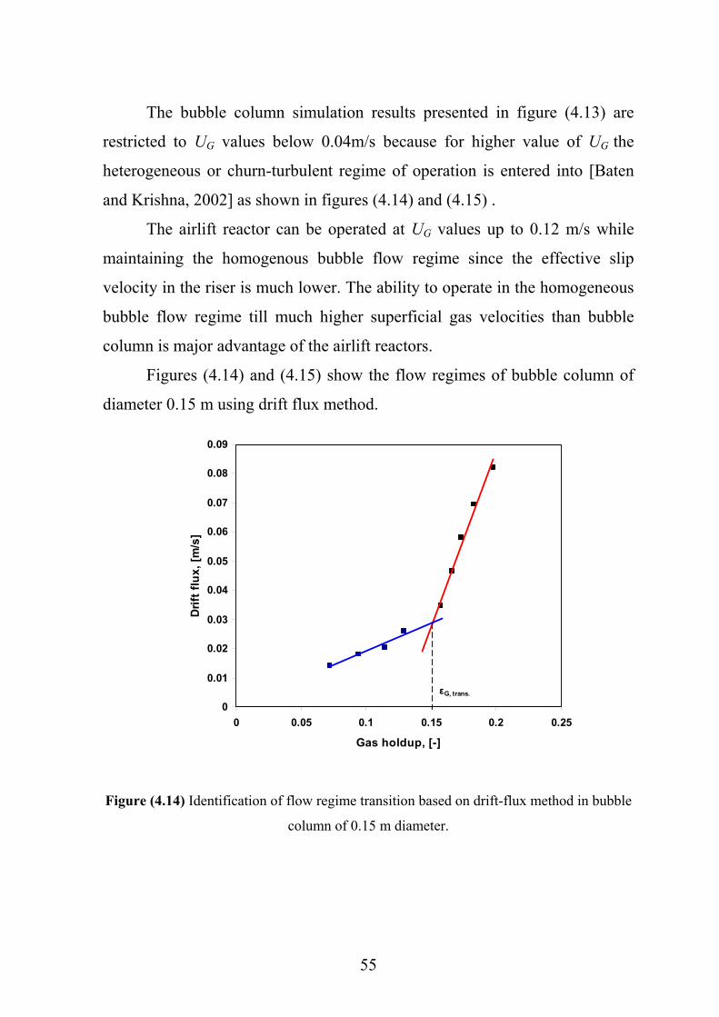
Figures (4.14) and (4.15) show the flow regimes of bubble column of
diameter 0.15 m using drift flux method.
0
0.01
0.02
0.03
0.04
0.05
0.06
0.07
0.08
0.09
0 0.05 0.1 0.15 0.2 0.25
Gas holdup, [-]
Drif
t flu
x, [m
/s]
εG, trans.
Figure (4.14) Identification of flow regime transition based on drift-flux method in bubble
column of 0.15 m diameter.
56
0
0.05
0.1
0.15
0.2
0.25
0 0.02 0.04 0.06 0.08 0.1 0.12
Superficial gas velocity, [m/s]
Gas
hol
dup,
[-]
UG, trans.
εG trans.
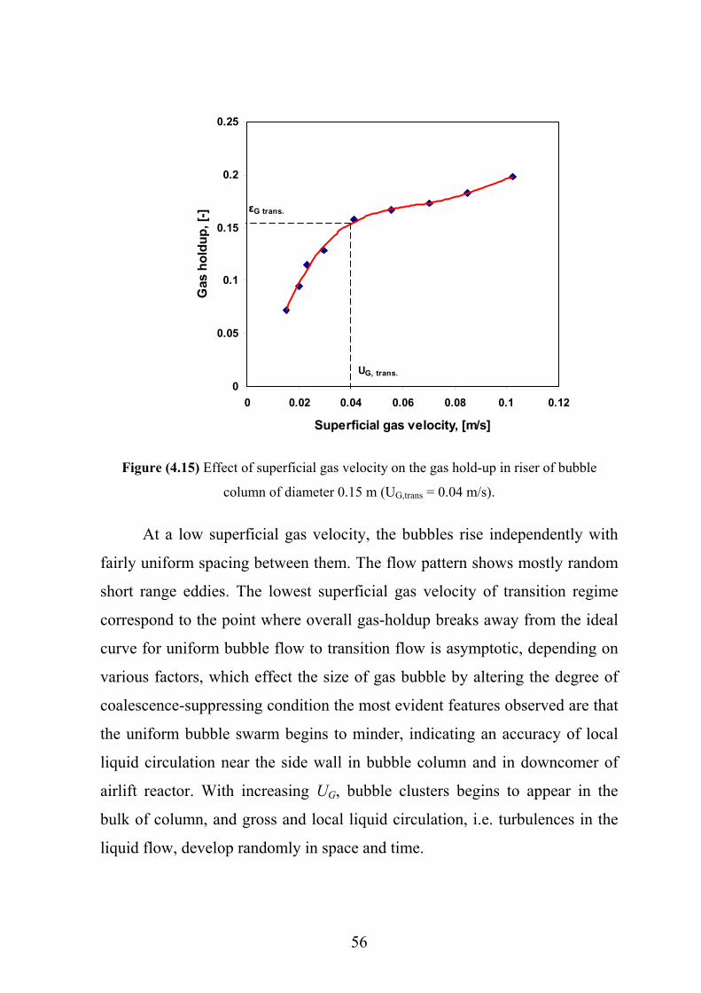
Figure (4.15) Effect of superficial gas velocity on the gas hold-up in riser of bubble
column of diameter 0.15 m (UG,trans = 0.04 m/s).
At a low superficial gas velocity, the bubbles rise independently with
fairly uniform spacing between them. The flow pattern shows mostly random
short range eddies. The lowest superficial gas velocity of transition regime
correspond to the point where overall gas-holdup breaks away from the ideal
curve for uniform bubble flow to transition flow is asymptotic, depending on
various factors, which effect the size of gas bubble by altering the degree of
coalescence-suppressing condition the most evident features observed are that
the uniform bubble swarm begins to minder, indicating an accuracy of local
liquid circulation near the side wall in bubble column and in downcomer of
airlift reactor. With increasing UG, bubble clusters begins to appear in the
bulk of column, and gross and local liquid circulation, i.e. turbulences in the
liquid flow, develop randomly in space and time.
57
In loop reactors, the regime transitions can be delayed up to much
higher superficial gas velocities, because of the effect of the overall liquid
velocity on the stability of the flow. The differences between regimes are less
apparent in airlift reactors as compared to bubble columns, due to the opposite
effects mentioned above.
58
CHAPTER FIVE
Conclusions and Recommendation for Future Work
5.1 Conclusions The following conclusions could be drawn from the work:
1. The gas and liquid phases show virtual plug flow behavior in the riser
of an airlift. This is contrast with bubble columns where both gas and
liquid phases deviate strongly from plug flow.
2. Due to the much lower slip between gas and liquid velocities in the
riser of the airlift, homogenous bubble flow can be maintained at much
higher UG values in airlifts than in bubble columns.
3. CFD simulation can be powerful tool for the modeling and design of
airlift and bubble column reactors, especially in the context of
describing the complex flow of the gas and liquid phases for different
geometrical configurations.
4. The transition regimes appears at high superficial gas velocity in airlift
reactors because of its ability to operate in the homogeneous bubble
flow regime till much higher superficial gas velocities than bubble
column is major advantage of the airlift reactors
5. Liquid flow velocities clearly showed the influence of superficial gas
velocity on liquid circulation in the reactor. The common radial profile
of axial liquid velocity far away from sparger and degassing zone
influence exhibits a parabolic to almost linear shape with an upflow
maximum in the center and a down flow region in down comer.
59
5.2 Recommendations for Future Work From the present study, it is noticed that further studies in the following areas
would be desired:
1. The effect of type of sparger on the gas holdup and liquid velocity.
2. The hydrodynamics of airlift reactors at high superficial gas velocity in
the riser.
3. Mixing in the airlift reactors.
4. Comparison of the hydrodynamics of internal and external loop in
airlift reactors.
5. The effect of using high liquid viscosity instead of water.
6. The effect of electrolyte and solid suspension on hydrodynamics of
airlift reactors.
60
REFERENCES
1. Abid Akhtar, Pareek, V., K., and Tade, M., O.," Modern Trends in CFD
Simulations: Application to GTL Technology", Chem. Prod. and Process
Modeling, Vol. 1, Issue 1, Article2, 2006.
2. Anderson, G., D., P., "Analysis of Currents and Mixing in a modified
Bubble Column Reactor", the Canadian society for engineering in
agricultural food, and biological system, no. 043071, 2004.
3. Baten, V. J. M., Krishna, R., Chem. Eng.Technol, 25, 1081, 2002.
4. Baten, V., J.M., and Krishna, R.," Comparison of hydrodynamic and Mass
Transfer in Airlift and Bubble Column Reactors Using CFD", Chem. Eng.
Techno, pp. (1047-1079), 2003.
5. Blazej, M., Glover, C., G.M., Generalis, S.C., and Markos, J., "Gas–Liquid
Simulation of an Airlift Bubble Column Reactor", Chem. Eng. and
Processing 43, 137–144, 2004.
6. Bohn, M., S., "First 3D Simulation of Bubble Column Hydrodynamics
Paves Way for Commercial Gas-to-Liquid Conversion in Slurry Reactor",
Vice President, Engineering, 2000.
7. Buwa, V., and Ranade, V., "Bubbling Columns", National chemical
laboratory, India, 2003.
8. Chen, R.C., Fan, L.-S., "Particle image velocimetry for characterizing the
low structure in three-dimensional gas-liquid-solid fluidized beds, 1992.
61
9. Chen, R.C., Reese, J., and Fan, F.-S., "Flow Structure in a Three-
Dimensional Bubble Column and a Three-Phase Fluidized Bed", AIChE
J., 40(7): 1093-1104, 1994.
10. Chisti and Molina," A reassesment of relationship between riser and down
comer gas holdups in airlift reactors ", Chem. Eng. Science, Vol. 53,
No.24, pp.4151-4154, 1998.
11. Chemical Industry of the Future Technology Roadmap for Computational
Fluid Dynamics, 1999.
12. Dautzenberg, F., M., and de Deken, J., C., "Reactor developments in
hydrotreating and conversion of residues", Catal. Rev. Sci. Eng., 26, 421,
1984.
13. Deckwer, W.-D., (1992): Bubble Column Reactors, J. Wiley & Son LTD,
Chichester.
14. Deen, N.G., Solberg, T., and Hjertager, B.H., "Numerical Simulation of
the Gas-Liquid Flow in a Square Cross sectioned Bubble Column",
http://hugin.aue.auc.dk,2000.
15. Delmas, H., Helene Chaumat, H., and Billet, A., "Axial and Radial
Investigation of Hydrodynamics in a Bubble Column; Influence of Fluids
Flow Rates and Sparger Type", Intentional Journal of Chem. Reactor
Eng., Vol. 4 2006 Article A25
62
16. Devanathan, N., "Investigation of Liquid Hydrodynamics in Bubble
Columns via Computer Automated Radioactive Particle Tracking
(CARPT) Facility", D.Sc. Thesis, Washington University, St. Louis,
Missouri, USA , 1991.
17. Diaz, E., M., Montes, F., J., and Galan, M., A.," Gas Liquid Flow in A
rectangular Partially Aerated Bubble Column:-Combined Effect Aspect
Ratio and Superficial Gas of Velocity", University of Salamanca,
Salamanca, Spain, 2006.
18. Dolgos, O., Klein, J., Vicente, A., A., Teixeira, J., A., "Behavior of dual
gas-liquid separator in an internal-loop airlift reactor –effect of top
clearance", 28th Conference SSCHE, 21 – 25 May, 2001.
19. Fan, L.-S., Luo, X., Tsuchiya, K., Lin, T.-S., Chen, Q., and Lee, D. J.,
"Progress in Understanding the Fluid Dynamics of Bubble Column
Reactors – II", Department of Chemical Engineering, The Ohio State
University 140 W. 19th Ave., Columbus, Ohio 43210 USA, 1998.
20. Franz, K., Borner, T., Kantoreck, H., and Buchcholz, R., "Flow structure
in bubble columns", Ger. Chem. Eng., 7, 365-374, 1984.
21. Geary, N.W. and Rice, R.G., "Bubble Size Prediction for Rigid and
Flexible Spargers ", AIChE J., Vol. 37, No. 2, pp.161-168, 1991 b.
22. Haidari, A., H., and matthews, "Future trends for computational fluid
dynamics in the process industry", third international conference on CFD
in the minerals and process industries, pp. (331), 2003.
63
23. Idogawa, K., Ikeda, K., Fukuda, T., and Morooka, S., Chem. Eng. Comm.,
59, 201, 1987.
24. Hills, J.H., "Radial Non-uniformity of Velocity and Voidage in a Bubble
Column", Trans. Inst. Chem. Eng., 52: 1-9 , 1975.
25. Joshi, J.B., Vitankar, V.S., Kulkarni, A.A., Dhotre, M.T., and Ekambara,
K., “Coherent Flow Structures in Bubble Column Reactors”, Chem. Eng.
Science, Vol. 57, pp. 3157-3183, 2002.
26. Kawase, Y.; Moo-Young, M., "Liquid Phase Mixing in Bubble Columns
with Newtonian and Non-Newtonian Fluids", Chem. Eng.Science 41,
1986.
27. Kelkar, Balmohan, G., "Flow regime characteristics in cocurrent bubble
column reactors. Chemical Engineering Communications, 41(1-6), 237-
251, 1986.
28. Klein, J., Vicente, A., A., and Teixeira , J., A., "Hydrodynamics of a
Three-phase Airlift Reactor with an Enlarged Separator – Application to
High Cell Density Systems", The Canadian Journal of Chemical
Engineering, Volume 81,August 2003 .
29. Krishna, R. and Baten, J. M. V., "Mass transfer of bubble columns",
Catalysis Today. 79- 80: 67-75, 2003.
64
30. Krishna, R., Urseanu, M. I., Baten, J. M. V., and Ellenberger, J., "Wall
effects on the rise of single gas bubbles in liquids" Int. Comm. Heat Mass
Transfer. 26(6): 781-790, 1999.
31. Kumar, D., "Design and Scale-Up of Bioreactors Using Computer
Simulations", Bioprocess International, 2006.
32. Kuzmin, D., and Turek, S.," Efficient numerical techniques for flow
simulation in bubble column reactor", University of Dortmund
Vogelpothsweg 87, D-44227 Dortmund, Germony, 1999.
33. Gobby, D., Hamill, I. S., Jones, I. P., Lewin, J., and Montavon, C.,
"Application of CFD to Multi-Phase Mixing", CFX, AEA Technology
Engineering Software, 2002.
34. Lain, S., Broder D., and Sommerfeld, M., "Numerical Modeling of the
Hydrodynamics in a Bubble Column Using the Euler-Lagrange Approach
", Universitat Halle-Wittenberg, D-O6099 Halle (Saale). Gerrnany, 2000.
35. Michele, V., "CFD Modeling and Measurement of Liquid Flow Structure
and Phase Holdup in Two- and Three-Phase Bubble Columns", der
Technischen Universit¨at Carolo-Wilhelmina zu Braunschweig, 2001.
36. Marchot, P., Fransolet, E., L'Homme, G., Crine, M., and Toye, D., "Gas
Liquid Solid Bubble Column Investigation by Electrical Resistance
Tomography", Laboratoire de Génie Chimique, B6, Université de Liège,
Liège B4000, Belgium, 2002.
65
37. Marchot, P., Fransolet, E., L'Homme, G., Crine, M., and Toye, D., "Gas
Liquid Solid Bubble Column Investigation by Electrical Resistance
Tomography", Université de Liège, Liège B4000, Belgium, 2001.
38. Martis, E.L.,"` Flow Regime Transitions in Bubble Column Reactors",
Augest, 2004.
39. Massimilla, L., Solimando, A., and Squillace, E., British Chemical
Engineering, April, 233, 1961.
40. Miron, A. S., Gomez, A. C., Camacho, F. G., Grima, E. M., and Chisti, Y.,
"Comparative evaluation of compact photobioreactors for large-scale
monoculture of microalgae" Journal of Biotechnology. 70: 249-270, 1999.
41. Miron, A. S., Camacho, F. G., Gomez, A. C., Grima, E. M., and Chisti, Y.
"Bubble- Column and Airlift Photobioreactors for Algal Culture"
American Institute of Chemical Engineers Journal. 46(9): 1872-1887,
2000.
42. Mouza, K., A., Kazakis, N., A., and Paras, S., V.,"Bubble Column Reactor
Design Using CFD Code", Laboratory of Chem. Process and Plant Design
Department of Chem. Eng. Aristotle University of Thessaloniki, 2004.
43. Nenes, A., Assimacopoulos, D., Markatos, N., and Mttsoulis, E.,
"Simulation of Airlift Pumps for Deep Water Wells", 1994.
66
44. Nguyena, K., Dawb, C.S., Chakkaa, P., Chenga, M., Brunsa, D.D.,
Finneya, C.E.A., Kennela, M.B., " Spatio-temporal dynamics in a train of
rising bubbles", Chemical Engineering Journal 64:1, 191-197, 1996.
45. Niels, G., Deen1, Esther I.V. van den Hengel1,2, Martin van Sint
Annaland1 and J.(Hans)A.M. Kuipers1," Multi-Scale Modeling of
Dispersed Gas-Liquid Two-Phase Flows ", 5th International Conference
on Multiphase Flow, ICMF’04 Yokohama, Japan, May 30–June 4, Paper
No. K07, 2004.
46. Olmos, E., Gentric, C., Vial, Ch., Wild, G., and Midoux, N., “Numerical
simulation of multiphase flow in bubble column reactors. Influence of
bubble coalescence and break-up”, Chemical Engineering Science, Vol.
56, pp. 6359-6365, 2001.
47. Olivieri, G., Marzocchella, A., Salatino, P., "Hydrodynamics of A Lab-
Scale Two-Phase Internal Loop Airlift Reactor", Dip. di Ingegneria
Chimica – Università degli Studi di Napoli Federico P.le Tecchio, 80 –
80125 Napoli, Italy , 2006.
48. Poulsen B. R., and Iversen, J. J. L., "Characterization of Gas Transfer and
Mixing in a Bubble Column Equipped with a Rubber Membrane Diffuser"
Biotechnology and Bioengineering. 58: 633-641, 1998.
49. Prince, M.J., and Blanch, H.W., "Bubble Coalescence and Break-up in
Air-Sparged Bubble Columns", AIChE J., Vol 36, No 10, pp 1485-1499,
1990.
67
50. http://www.Process technology computational fluid dynamics at
BHRSolutions.htm
51. Ruzicka, M. C.; Zahradnik, J.; Drahos, J.; Thomas, N. H., "Homogeneous-
heterogeneous regime transition in bubble columns. Chemical Engineering
Science, 56(15), 4609-4626, (2001).
52. Sa´nchezMiro´n,A., Contreras Go´mez,A., Garcı´a Camacho, F.,
MolinaGrima, E. and Chisti, Y., 1999, Comparative evaluation of compact
photobioreactors for large-scale monoculture of microalgae, J Biotechnol,
70: 249–270.
53. Sa´nchez Miro´n, A., Garcı´a Camacho, F., Contreras Go´mez, A., Molina
Grima, E. and Chisti, Y., 2000, Bubble column and airlift photobioreactors
for algal culture, AIChE J, 46: 1872–1887.
54. Sarrafi, Amir; Jamialahmadi, Mohammad; Muller-Steinhagen, Hans;
Smith, John M., "Gas holdup in homogeneous and heterogeneous gas-
liquid bubble column reactors. Canadian Journal of Chemical Engineering,
77(1), 11-21, 1999.
55. Shun and Yasuhiro, "Gas-phase dispersion in bubble columns ", Chem.
Eng. Science, Vol.45, No. 4, pp.901-905, 1990.
56. Shaikh, A., and Al-Dahhan, M., H., "A Review on Flow Regime
Transition in Bubble Columns", International journal of chemical reactor
engineering, Vol. 5, Review R1, 2007.
68
57. Silva, R., Neto1, S., and Vilar, E., "A Computational Fluid Dynamics
Study of Hydrogen Bubbles in an Electrochemical Reactor", Brazilian
Archives of Biology and Technology Journal, Vol.48, Special n.: pp. 219-
229, June 2005.
58. Simon Lo," Application of Population Balance to CFD Modeling of Gas-
Liquid Reactors", Trends in Numerical and Physical Modeling for
Industrial Multiphase Flow, 2000.
59. Solbakken, T., and Hjertager, B., H., "A Computational and Experimental
Study of Flow Pattern in a pilot and Full Scale Bubble Column", Third
International Conference On Multiphase Flow, ICMF’98 Lyon, France,
June 8-12, 1998.
60. Taitel, Y., D. Bornea and A.E. Buckler, "Modelling Flow Pattern
Transitions for Steady Upward Gas-Liquid Flow in Vertical Tubes",
AIChE J. 26, 345-354, 1980.
61. Tharat, B. N. ; Shevad, A. V.; Bhilegaovkar, K. V.; Aglawe, R. H.; Parasu,
U.; Thakre, S. S.; Pandit, A. B.; Sawant, S. B.; and Joshi, J. B., "Effect of
sparger design and height to diameter ratio on fractional gas holdup in
bubble column ", Trans. I. Chem., vol. 76, part A,October,1998.
62. Urseanu M. L. and Krishna, R., "Scaling up Bubble Column Reactors"
Unpublished Ph.D. Thesis. Amsterdam, The Netherlands.: University of
Amsterdam, Department of Chemical Engineering, 2000.
69
63. Vatai, GY., and Tekic, M.N.,"Gas-Holdup and Mass Transfer in Bubble
Columns with Pseudo Plastic Liquids", hem. Eng. Science, Vol. 44, No.
10, pp. 2402-2407, 1989.
64. Viswanathan, K., Rao, S., D., "Circulation in bubble columns", Chem.
Eng. Sceince, Vol. 38, No.3, pp. 474-478, 1983.
65. Vladimir and Andrei," CFD Modeling of Gas-Liquid Flows in Water
Electrolysis Units", Stuart Energy Systems Corporation 5101 Orbitor
Drive, Mississauga ON L4W 4V1, CANADA, 2003.
66. Wallis, G. B., "One Dimensional Two Phase Flow", McGraw Hill, New
York, 1969.
67. Wang, B., Rehm, W., Jülich, F., "Overview of Models for Multifluid
/Multiphase Flows Based on CFD Codes D3UNS, CFX-5, IFSAS with
Test Cases for Complex Flows (Part -2)", Forschungszentrum Jülich,
Germany,2003.
68. Wild, G., Li, H.Z., Poncin, S., and Olmos, E., “Some Aspects of the
Hydrodynamics of Bubble Columns”, International Journal of Chem.
Reactor Eng., Vol. 1, pp. 1-36, 2003.
69. Wilkinson, Peter M.; Spek, Arie P.; Van Dierendonck, Laurent L., "Design
parameters estimation for scaleup of high-pressure bubble columns"
AIChE Journal, 38(4), 544-54, 1992.
70
70. Wouter, "Splendid science", Harteveld - Department of Multi-Scale
Physics, 2006.
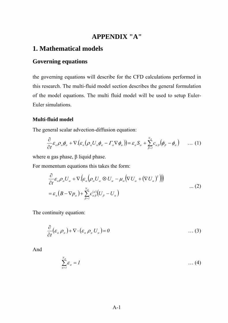
A-1
APPENDIX "A"
1. Mathematical models
Governing equations
the governing equations will describe for the CFD calculations performed in
this research. The multi-fluid model section describes the general formulation
of the model equations. The multi fluid model will be used to setup Euler-
Euler simulations.
Multi-fluid model
The general scalar advection-diffusion equation:
( )( ) ( )αββ
βαααααααααααα φφεφΓφρεφρε −+=∇−∇+∂∂
∑=
pN
1cSU.
t … (1)
where α gas phase, β liquid phase.
For momentum equations this takes the form:
( )( )( )( )
( ) ( ) ( )∑=
−+∇−=
∇+∇−⊗∇+∂∂
pN
1
d
T
UUcpB
UUUU.Ut
βαββααα
αααααααααα
ε
µρερε ... (2)
The continuity equation:
( ) ( ) 0Ut
=⋅∇+∂∂
ααααα ρερε … (3)
And
1pN
1=∑
=ααε … (4)
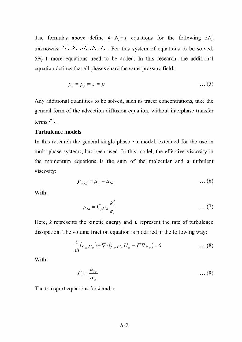
A-2
The formulas above define 4 Np+1 equations for the following 5Np
unknowns: . For this system of equations to be solved,
5Np-1 more equations need to be added. In this research, the additional
equation defines that all phases share the same pressure field:
p...pp === βα … (5)
Any additional quantities to be solved, such as tracer concentrations, take the
general form of the advection diffusion equation, without interphase transfer
terms .
Turbulence models
In this research the general single phase model, extended for the use in
multi-phase systems, has been used. In this model, the effective viscosity in
the momentum equations is the sum of the molecular and a turbulent
viscosity:
ααα µµµ Teff, += … (6)
With:
α
ααµα ε
ρµ2
T
kC= … (7)
Here, k represents the kinetic energy and represent the rate of turbulence
dissipation. The volume fraction equation is modified in the following way:
( ) ( ) 0Ut
=∇−⋅∇+∂∂
αααααα εΓρερε … (8)
With:
α
αα σ
µΓ T= … (9)
The transport equations for k and ε:
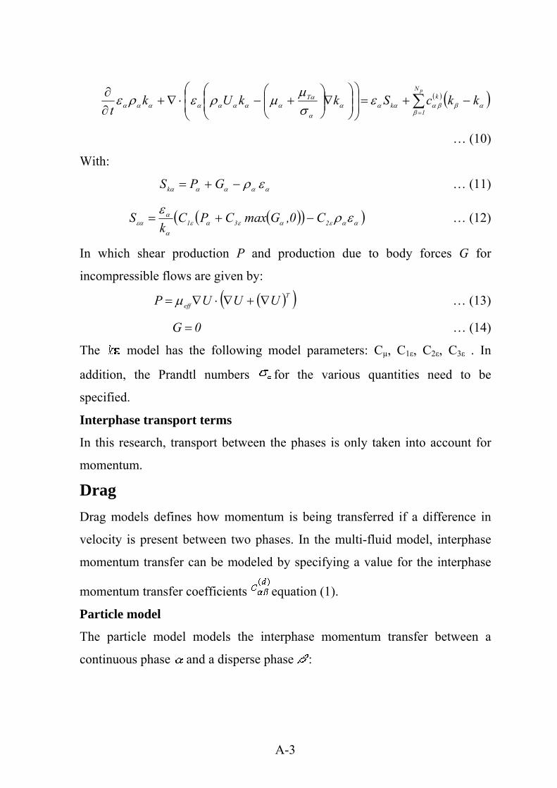
A-3
( ) ( )αββ
βααααα
ααααααααα ε
σµµρερε kkcSkkUk
t
pN
1
kk
T −+=⎟⎟⎠
⎞⎜⎜⎝
⎛⎟⎟⎠
⎞⎜⎜⎝
⎛∇⎟⎟⎠
⎞⎜⎜⎝
⎛+−⋅∇+
∂∂ ∑
=
… (10)
With:
ααααα ερ−+= GPSk … (11)
( )( )( )ααεαεαεα
αεα ερε
231 C0,GmaxCPCk
S −+= … (12)
In which shear production P and production due to body forces G for
incompressible flows are given by:
( )( )Teff UUUP ∇+∇⋅∇= µ … (13)
0G = … (14)
The model has the following model parameters: Cµ, C1ε, C2ε, C3ε . In
addition, the Prandtl numbers for the various quantities need to be
specified.
Interphase transport terms
In this research, transport between the phases is only taken into account for
momentum.
Drag Drag models defines how momentum is being transferred if a difference in
velocity is present between two phases. In the multi-fluid model, interphase
momentum transfer can be modeled by specifying a value for the interphase
momentum transfer coefficients equation (1).
Particle model
The particle model models the interphase momentum transfer between a
continuous phase and a disperse phase :
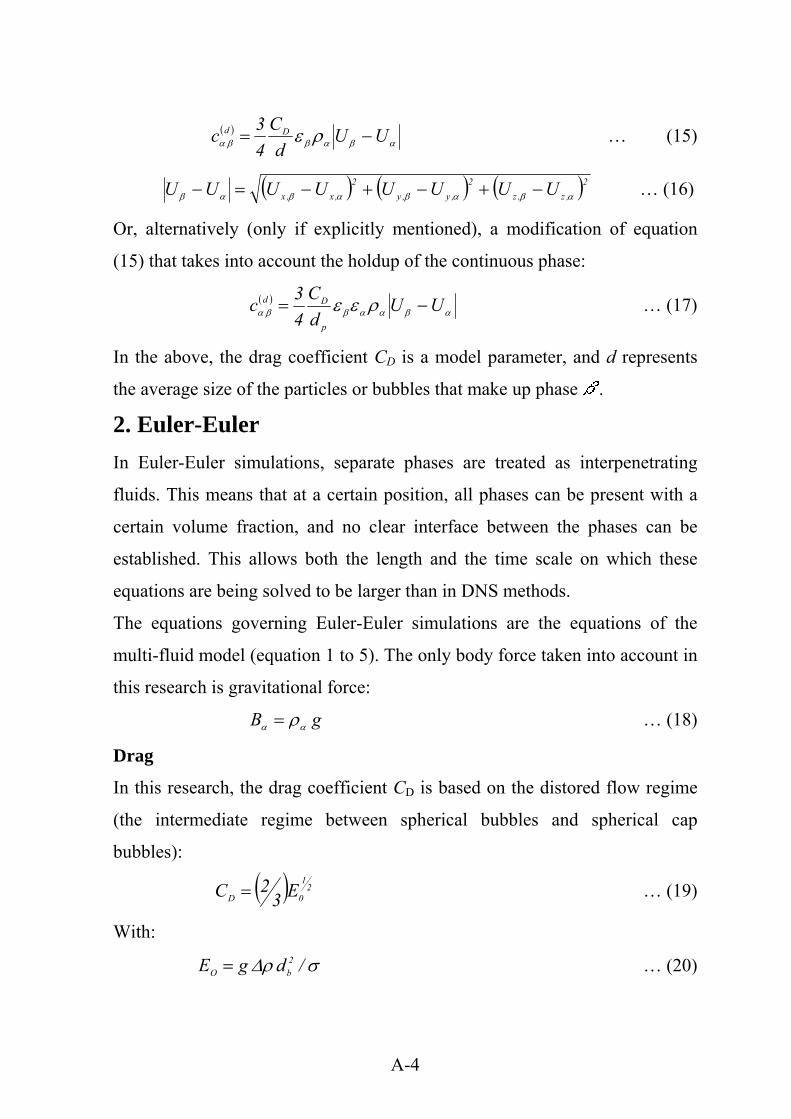
A-4
( )αβαββα ρε UU
dC
43c Dd −= … (15)
( ) ( ) ( )2,z,z
2,y,y
2,x,x UUUUUUUU αβαβαβαβ −+−+−=− … (16)
Or, alternatively (only if explicitly mentioned), a modification of equation
(15) that takes into account the holdup of the continuous phase:
( )αβααββα ρεε UU
dC
43c
p
Dd −= … (17)
In the above, the drag coefficient CD is a model parameter, and d represents
the average size of the particles or bubbles that make up phase .
2. Euler-Euler In Euler-Euler simulations, separate phases are treated as interpenetrating
fluids. This means that at a certain position, all phases can be present with a
certain volume fraction, and no clear interface between the phases can be
established. This allows both the length and the time scale on which these
equations are being solved to be larger than in DNS methods.
The equations governing Euler-Euler simulations are the equations of the
multi-fluid model (equation 1 to 5). The only body force taken into account in
this research is gravitational force:
gB αα ρ= … (18)
Drag
In this research, the drag coefficient CD is based on the distored flow regime
(the intermediate regime between spherical bubbles and spherical cap
bubbles):
( ) 21
0D E32C = … (19)
With:
σρ∆ /dgE 2bO = … (20)
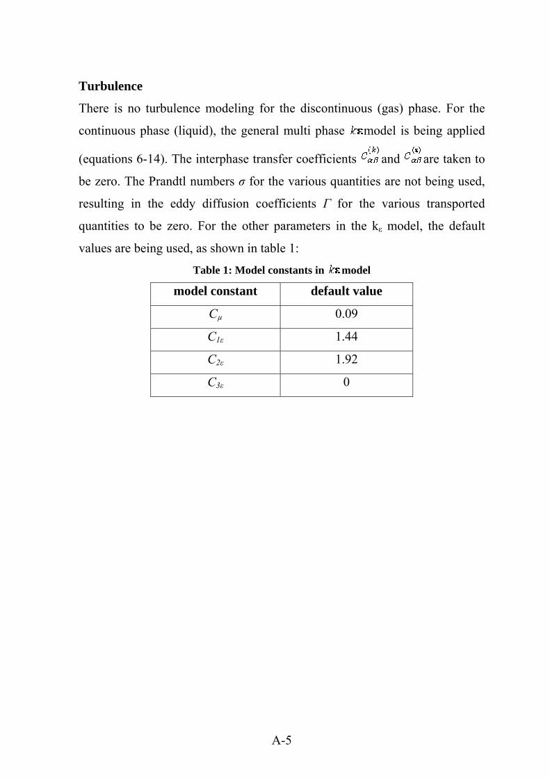
A-5
Turbulence
There is no turbulence modeling for the discontinuous (gas) phase. For the
continuous phase (liquid), the general multi phase model is being applied
(equations 6-14). The interphase transfer coefficients and are taken to
be zero. The Prandtl numbers σ for the various quantities are not being used,
resulting in the eddy diffusion coefficients Γ for the various transported
quantities to be zero. For the other parameters in the kε model, the default
values are being used, as shown in table 1:
Table 1: Model constants in model
model constant default value
Cµ 0.09
C1ε 1.44
C2ε 1.92
C3ε 0
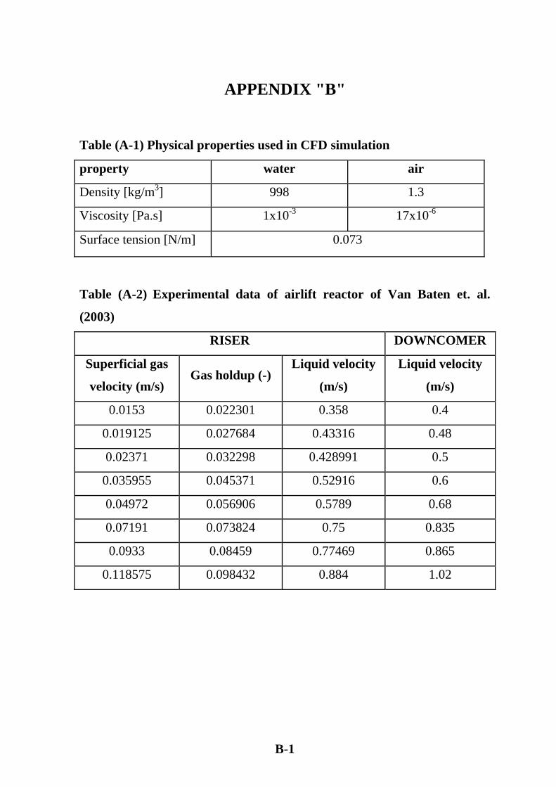
B-1
APPENDIX "B"
Table (A-1) Physical properties used in CFD simulation
property water air
Density [kg/m3] 998 1.3
Viscosity [Pa.s] 1x10⁻³ 17x10-6
Surface tension [N/m] 0.073
Table (A-2) Experimental data of airlift reactor of Van Baten et. al.
(2003)
RISER DOWNCOMER
Superficial gas
velocity (m/s) Gas holdup (-)
Liquid velocity
(m/s)
Liquid velocity
(m/s)
0.0153 0.022301 0.358 0.4
0.019125 0.027684 0.43316 0.48
0.02371 0.032298 0.428991 0.5
0.035955 0.045371 0.52916 0.6
0.04972 0.056906 0.5789 0.68
0.07191 0.073824 0.75 0.835
0.0933 0.08459 0.77469 0.865
0.118575 0.098432 0.884 1.02
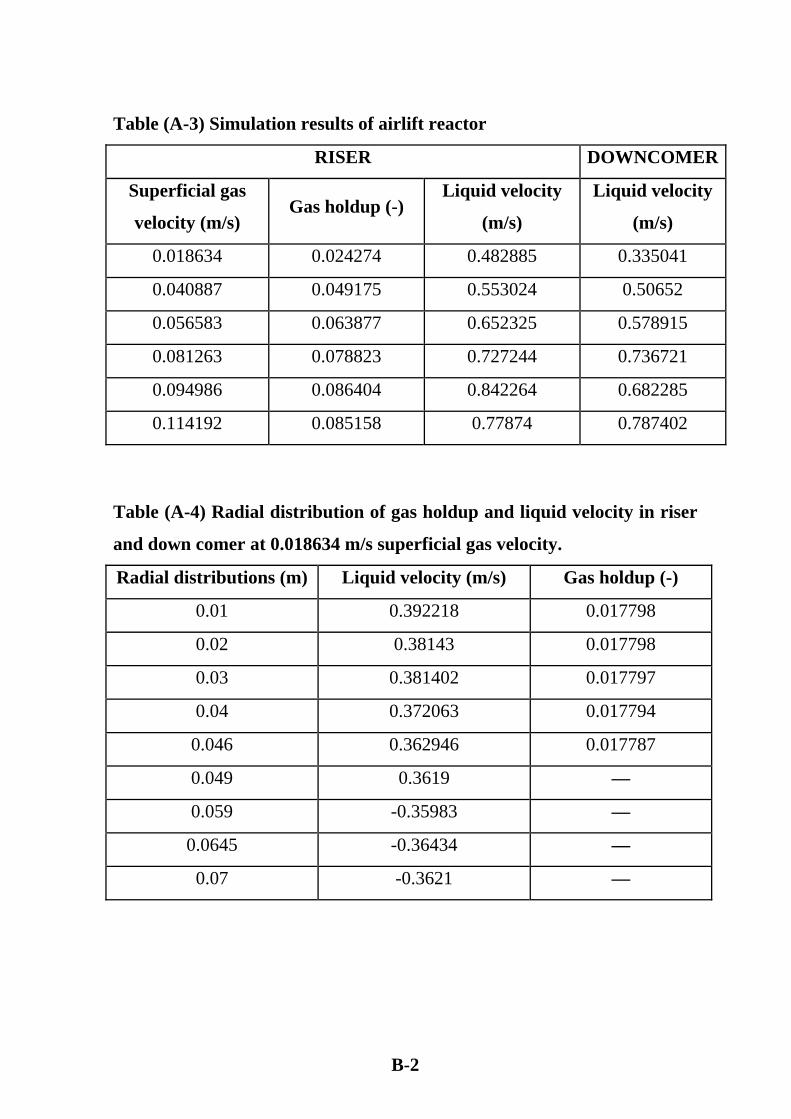
B-2
Table (A-3) Simulation results of airlift reactor
RISER DOWNCOMER
Superficial gas
velocity (m/s) Gas holdup (-)
Liquid velocity
(m/s)
Liquid velocity
(m/s)
0.018634 0.024274 0.482885 0.335041
0.040887 0.049175 0.553024 0.50652
0.056583 0.063877 0.652325 0.578915
0.081263 0.078823 0.727244 0.736721
0.094986 0.086404 0.842264 0.682285
0.114192 0.085158 0.77874 0.787402
Table (A-4) Radial distribution of gas holdup and liquid velocity in riser
and down comer at 0.018634 m/s superficial gas velocity.
Radial distributions (m) Liquid velocity (m/s) Gas holdup (-)
0.01 0.392218 0.017798
0.02 0.38143 0.017798
0.03 0.381402 0.017797
0.04 0.372063 0.017794
0.046 0.362946 0.017787
0.049 0.3619 —
0.059 -0.35983 —
0.0645 -0.36434 —
0.07 -0.3621 —
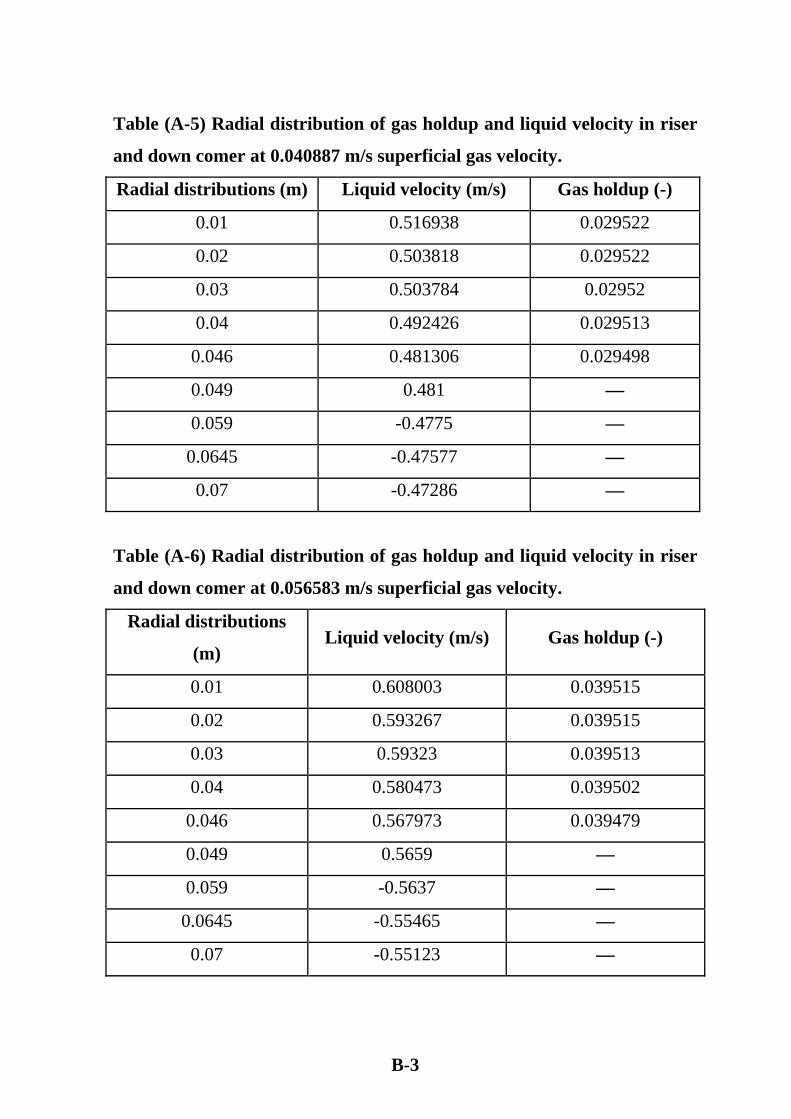
B-3
Table (A-5) Radial distribution of gas holdup and liquid velocity in riser
and down comer at 0.040887 m/s superficial gas velocity.
Radial distributions (m) Liquid velocity (m/s) Gas holdup (-)
0.01 0.516938 0.029522
0.02 0.503818 0.029522
0.03 0.503784 0.02952
0.04 0.492426 0.029513
0.046 0.481306 0.029498
0.049 0.481 —
0.059 -0.4775 —
0.0645 -0.47577 —
0.07 -0.47286 —
Table (A-6) Radial distribution of gas holdup and liquid velocity in riser
and down comer at 0.056583 m/s superficial gas velocity.
Radial distributions
(m) Liquid velocity (m/s) Gas holdup (-)
0.01 0.608003 0.039515
0.02 0.593267 0.039515
0.03 0.59323 0.039513
0.04 0.580473 0.039502
0.046 0.567973 0.039479
0.049 0.5659 —
0.059 -0.5637 —
0.0645 -0.55465 —
0.07 -0.55123 —
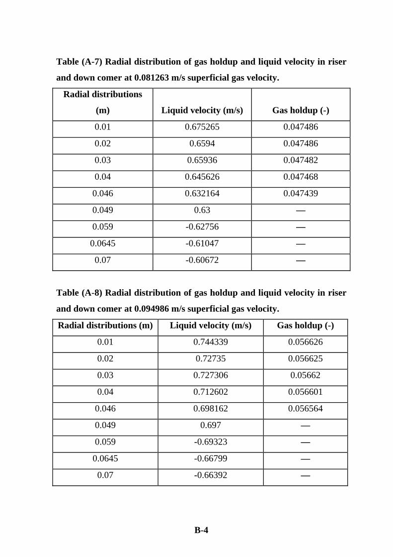
B-4
Table (A-7) Radial distribution of gas holdup and liquid velocity in riser
and down comer at 0.081263 m/s superficial gas velocity.
Radial distributions
(m) Liquid velocity (m/s) Gas holdup (-)
0.01 0.675265 0.047486
0.02 0.6594 0.047486
0.03 0.65936 0.047482
0.04 0.645626 0.047468
0.046 0.632164 0.047439
0.049 0.63 —
0.059 -0.62756 —
0.0645 -0.61047 —
0.07 -0.60672 —
Table (A-8) Radial distribution of gas holdup and liquid velocity in riser
and down comer at 0.094986 m/s superficial gas velocity.
Radial distributions (m) Liquid velocity (m/s) Gas holdup (-)
0.01 0.744339 0.056626
0.02 0.72735 0.056625
0.03 0.727306 0.05662
0.04 0.712602 0.056601
0.046 0.698162 0.056564
0.049 0.697 —
0.059 -0.69323 —
0.0645 -0.66799 —
0.07 -0.66392 —
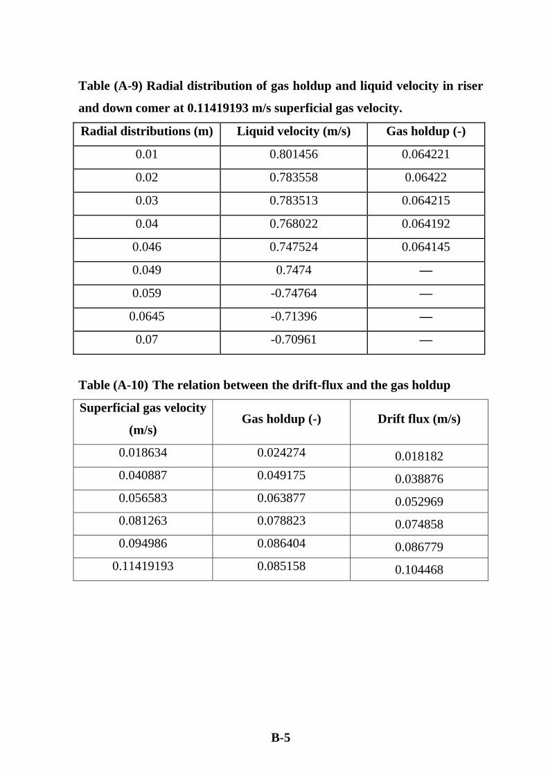
B-5
Table (A-9) Radial distribution of gas holdup and liquid velocity in riser
and down comer at 0.11419193 m/s superficial gas velocity.
Radial distributions (m) Liquid velocity (m/s) Gas holdup (-)
0.01 0.801456 0.064221
0.02 0.783558 0.06422
0.03 0.783513 0.064215
0.04 0.768022 0.064192
0.046 0.747524 0.064145
0.049 0.7474 —
0.059 -0.74764 —
0.0645 -0.71396 —
0.07 -0.70961 —
Table (A-10) The relation between the drift-flux and the gas holdup Superficial gas velocity
(m/s) Gas holdup (-) Drift flux (m/s)
0.018634 0.024274 0.018182 0.040887 0.049175 0.038876 0.056583 0.063877 0.052969 0.081263 0.078823 0.074858 0.094986 0.086404 0.086779
0.11419193 0.085158 0.104468
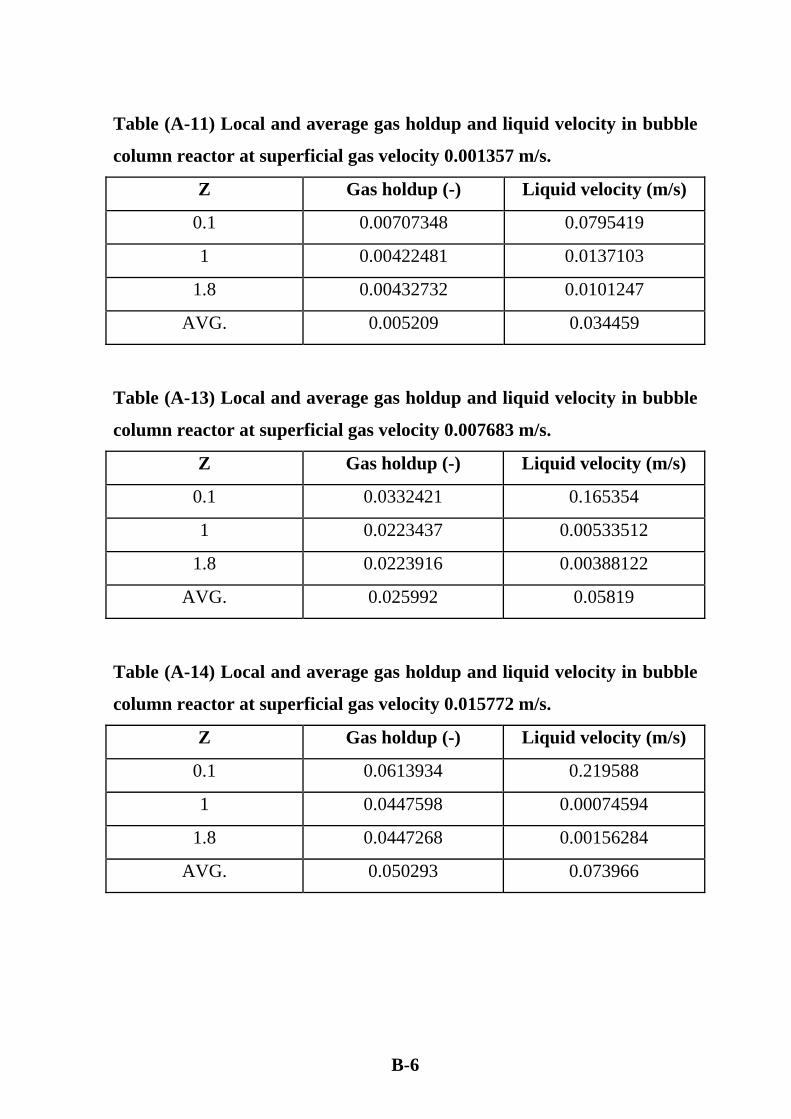
B-6
Table (A-11) Local and average gas holdup and liquid velocity in bubble
column reactor at superficial gas velocity 0.001357 m/s.
Z Gas holdup (-) Liquid velocity (m/s)
0.1 0.00707348 0.0795419
1 0.00422481 0.0137103
1.8 0.00432732 0.0101247
AVG. 0.005209 0.034459
Table (A-13) Local and average gas holdup and liquid velocity in bubble
column reactor at superficial gas velocity 0.007683 m/s.
Z Gas holdup (-) Liquid velocity (m/s)
0.1 0.0332421 0.165354
1 0.0223437 0.00533512
1.8 0.0223916 0.00388122
AVG. 0.025992 0.05819
Table (A-14) Local and average gas holdup and liquid velocity in bubble
column reactor at superficial gas velocity 0.015772 m/s.
Z Gas holdup (-) Liquid velocity (m/s)
0.1 0.0613934 0.219588
1 0.0447598 0.00074594
1.8 0.0447268 0.00156284
AVG. 0.050293 0.073966
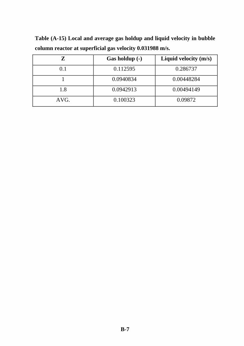
B-7
Table (A-15) Local and average gas holdup and liquid velocity in bubble
column reactor at superficial gas velocity 0.031988 m/s. Z Gas holdup (-) Liquid velocity (m/s)
0.1 0.112595 0.286737
1 0.0940834 0.00448284
1.8 0.0942913 0.00494149
AVG. 0.100323 0.09872
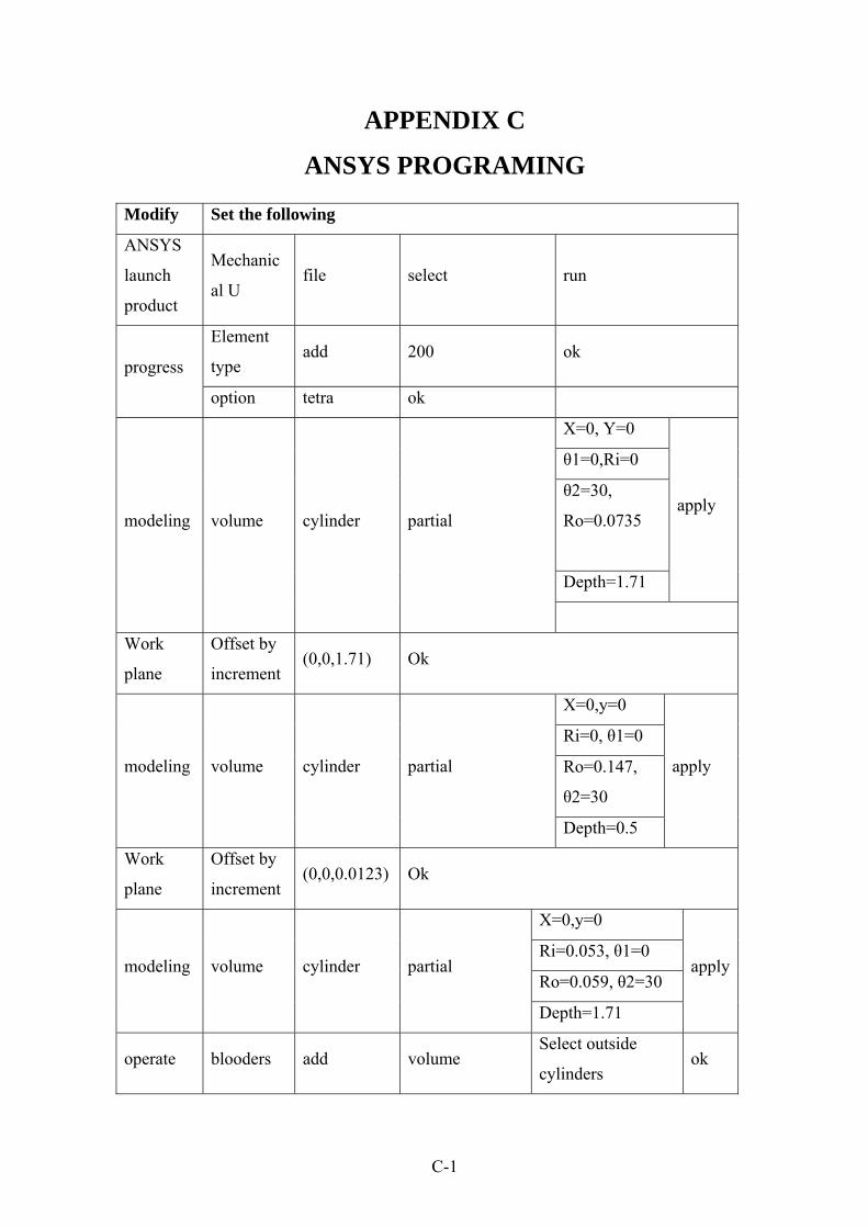
C-1
APPENDIX C
ANSYS PROGRAMING
Modify Set the following
ANSYS
launch
product
Mechanic
al U file select run
progress
Element
type add 200 ok
option tetra ok
modeling volume cylinder partial
X=0, Y=0
apply
θ1=0,Ri=0
θ2=30,
Ro=0.0735
Depth=1.71
Work
plane
Offset by
increment (0,0,1.71) Ok
modeling volume cylinder partial
X=0,y=0
apply
Ri=0, θ1=0
Ro=0.147,
θ2=30
Depth=0.5
Work
plane
Offset by
increment (0,0,0.0123) Ok
modeling volume cylinder partial
X=0,y=0
applyRi=0.053, θ1=0
Ro=0.059, θ2=30
Depth=1.71
operate blooders add volume Select outside
cylinders ok
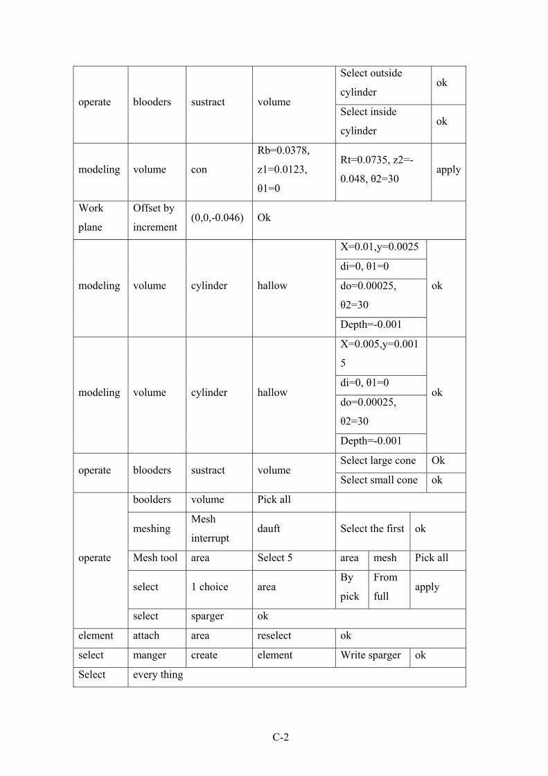
C-2
operate blooders sustract volume
Select outside
cylinder ok
Select inside
cylinder ok
modeling volume con
Rb=0.0378,
z1=0.0123,
θ1=0
Rt=0.0735, z2=-
0.048, θ2=30 apply
Work
plane
Offset by
increment (0,0,-0.046) Ok
modeling volume cylinder hallow
X=0.01,y=0.0025
ok
di=0, θ1=0
do=0.00025,
θ2=30
Depth=-0.001
modeling volume cylinder hallow
X=0.005,y=0.001
5
ok di=0, θ1=0
do=0.00025,
θ2=30
Depth=-0.001
operate blooders sustract volume Select large cone Ok
Select small cone ok
operate
boolders volume Pick all
meshing Mesh
interrupt dauft Select the first ok
Mesh tool area Select 5 area mesh Pick all
select 1 choice area By
pick
From
full apply
select sparger ok
element attach area reselect ok
select manger create element Write sparger ok
Select every thing
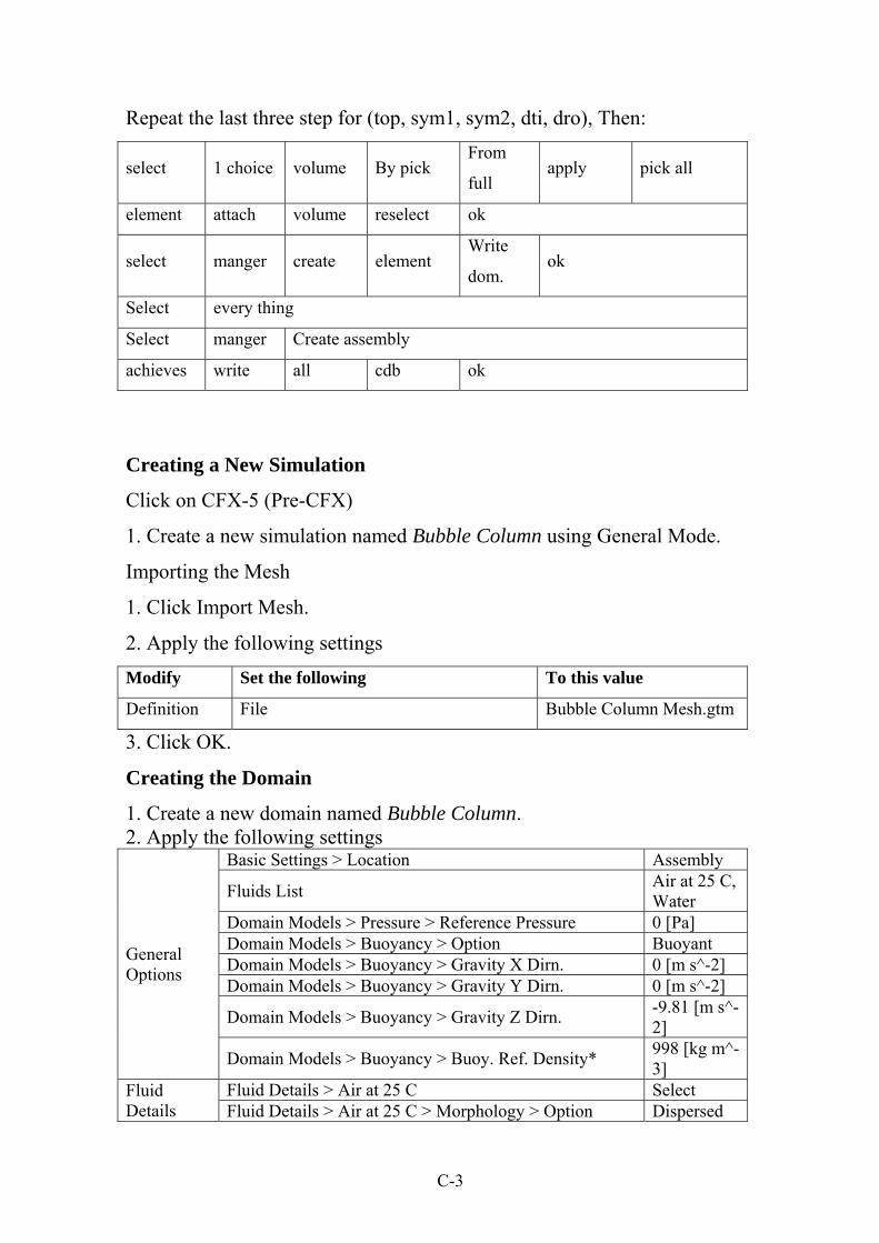
C-3
Repeat the last three step for (top, sym1, sym2, dti, dro), Then:
select 1 choice volume By pick From
full apply pick all
element attach volume reselect ok
select manger create element Write
dom. ok
Select every thing
Select manger Create assembly
achieves write all cdb ok
Creating a New Simulation
Click on CFX-5 (Pre-CFX)
1. Create a new simulation named Bubble Column using General Mode.
Importing the Mesh
1. Click Import Mesh.
2. Apply the following settings Modify Set the following To this value
Definition File Bubble Column Mesh.gtm
3. Click OK.
Creating the Domain
1. Create a new domain named Bubble Column. 2. Apply the following settings
General Options
Basic Settings > Location Assembly
Fluids List Air at 25 C, Water
Domain Models > Pressure > Reference Pressure 0 [Pa] Domain Models > Buoyancy > Option Buoyant Domain Models > Buoyancy > Gravity X Dirn. 0 [m s^-2] Domain Models > Buoyancy > Gravity Y Dirn. 0 [m s^-2]
Domain Models > Buoyancy > Gravity Z Dirn. -9.81 [m s^-2]
Domain Models > Buoyancy > Buoy. Ref. Density* 998 [kg m^-3]
Fluid Details
Fluid Details > Air at 25 C Select Fluid Details > Air at 25 C > Morphology > Option Dispersed
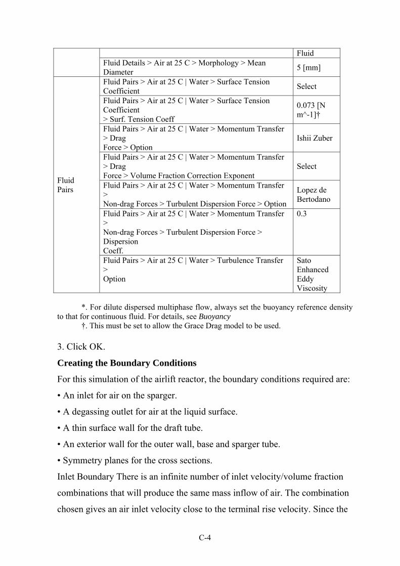
C-4
Fluid Fluid Details > Air at 25 C > Morphology > Mean Diameter 5 [mm]
Fluid Pairs
Fluid Pairs > Air at 25 C | Water > Surface Tension Coefficient Select
Fluid Pairs > Air at 25 C | Water > Surface Tension Coefficient > Surf. Tension Coeff
0.073 [N m^-1]†
Fluid Pairs > Air at 25 C | Water > Momentum Transfer > Drag Force > Option
Ishii Zuber
Fluid Pairs > Air at 25 C | Water > Momentum Transfer > Drag Force > Volume Fraction Correction Exponent
Select
Fluid Pairs > Air at 25 C | Water > Momentum Transfer > Non-drag Forces > Turbulent Dispersion Force > Option
Lopez de Bertodano
Fluid Pairs > Air at 25 C | Water > Momentum Transfer > Non-drag Forces > Turbulent Dispersion Force > Dispersion Coeff.
0.3
Fluid Pairs > Air at 25 C | Water > Turbulence Transfer > Option
Sato Enhanced Eddy Viscosity
*. For dilute dispersed multiphase flow, always set the buoyancy reference density
to that for continuous fluid. For details, see Buoyancy †. This must be set to allow the Grace Drag model to be used.
3. Click OK.
Creating the Boundary Conditions
For this simulation of the airlift reactor, the boundary conditions required are:
• An inlet for air on the sparger.
• A degassing outlet for air at the liquid surface.
• A thin surface wall for the draft tube.
• An exterior wall for the outer wall, base and sparger tube.
• Symmetry planes for the cross sections.
Inlet Boundary There is an infinite number of inlet velocity/volume fraction
combinations that will produce the same mass inflow of air. The combination
chosen gives an air inlet velocity close to the terminal rise velocity. Since the
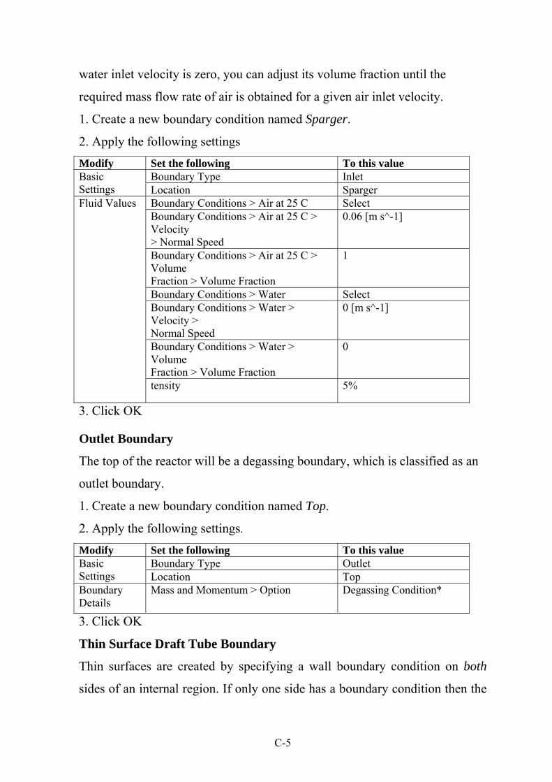
C-5
water inlet velocity is zero, you can adjust its volume fraction until the
required mass flow rate of air is obtained for a given air inlet velocity.
1. Create a new boundary condition named Sparger.
2. Apply the following settings Modify Set the following To this value Basic Settings
Boundary Type Inlet Location Sparger
Fluid Values Boundary Conditions > Air at 25 C Select Boundary Conditions > Air at 25 C > Velocity > Normal Speed
0.06 [m s^-1]
Boundary Conditions > Air at 25 C > Volume Fraction > Volume Fraction
1
Boundary Conditions > Water Select Boundary Conditions > Water > Velocity > Normal Speed
0 [m s^-1]
Boundary Conditions > Water > Volume Fraction > Volume Fraction
0
tensity 5%
3. Click OK Outlet Boundary
The top of the reactor will be a degassing boundary, which is classified as an
outlet boundary.
1. Create a new boundary condition named Top.
2. Apply the following settings.
Modify Set the following To this value Basic Settings
Boundary Type Outlet Location Top
Boundary Details
Mass and Momentum > Option
Degassing Condition*
3. Click OK
Thin Surface Draft Tube Boundary
Thin surfaces are created by specifying a wall boundary condition on both
sides of an internal region. If only one side has a boundary condition then the
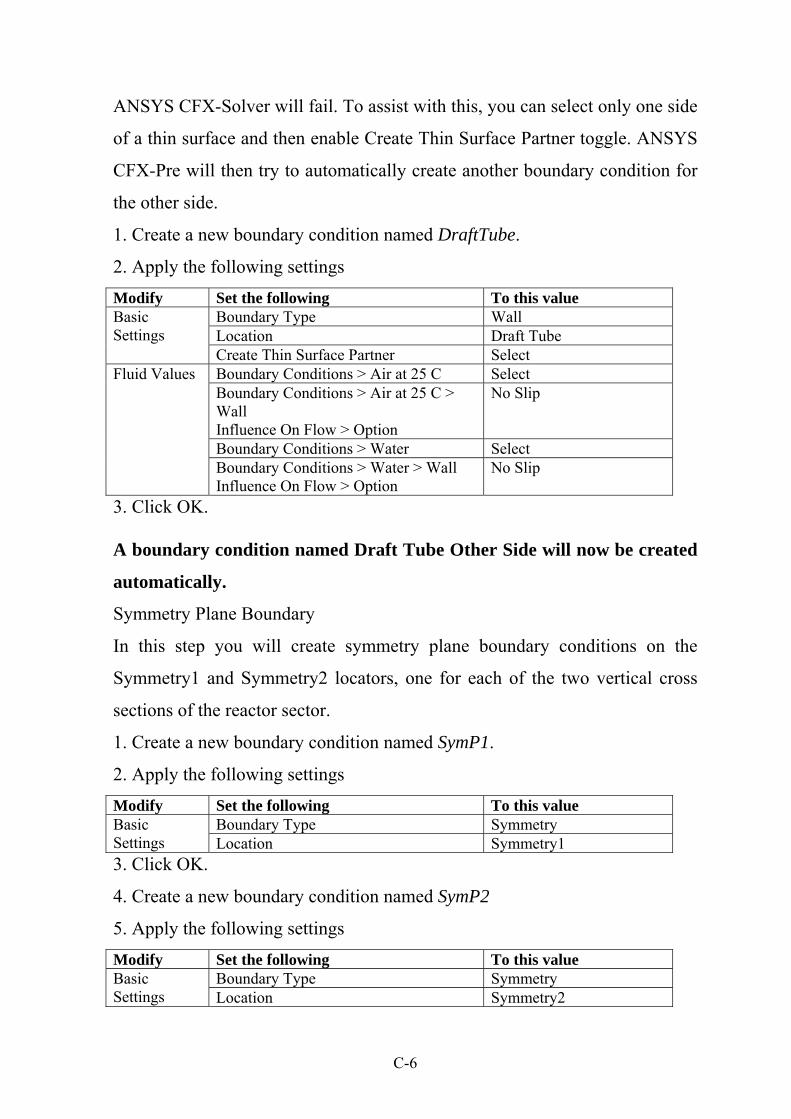
C-6
ANSYS CFX-Solver will fail. To assist with this, you can select only one side
of a thin surface and then enable Create Thin Surface Partner toggle. ANSYS
CFX-Pre will then try to automatically create another boundary condition for
the other side.
1. Create a new boundary condition named DraftTube.
2. Apply the following settings
Modify Set the following To this value Basic Settings
Boundary Type Wall Location Draft Tube Create Thin Surface Partner Select
Fluid Values Boundary Conditions > Air at 25 C Select Boundary Conditions > Air at 25 C > Wall Influence On Flow > Option
No Slip
Boundary Conditions > Water Select Boundary Conditions > Water > Wall Influence On Flow > Option
No Slip
3. Click OK. A boundary condition named Draft Tube Other Side will now be created
automatically.
Symmetry Plane Boundary
In this step you will create symmetry plane boundary conditions on the
Symmetry1 and Symmetry2 locators, one for each of the two vertical cross
sections of the reactor sector.
1. Create a new boundary condition named SymP1.
2. Apply the following settings Modify Set the following To this value Basic Settings
Boundary Type Symmetry Location Symmetry1
3. Click OK.
4. Create a new boundary condition named SymP2
5. Apply the following settings Modify Set the following To this value Basic Settings
Boundary Type Symmetry Location Symmetry2
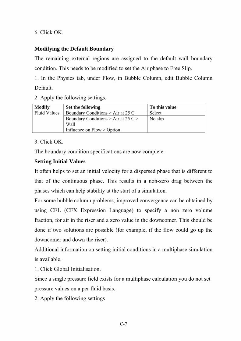
C-7
6. Click OK.
Modifying the Default Boundary
The remaining external regions are assigned to the default wall boundary
condition. This needs to be modified to set the Air phase to Free Slip.
1. In the Physics tab, under Flow, in Bubble Column, edit Bubble Column
Default.
2. Apply the following settings. Modify Set the following To this value Fluid Values Boundary Conditions > Air at 25 C Select
Boundary Conditions > Air at 25 C > Wall Influence on Flow > Option
No slip
3. Click OK.
The boundary condition specifications are now complete.
Setting Initial Values
It often helps to set an initial velocity for a dispersed phase that is different to
that of the continuous phase. This results in a non-zero drag between the
phases which can help stability at the start of a simulation.
For some bubble column problems, improved convergence can be obtained by
using CEL (CFX Expression Language) to specify a non zero volume
fraction, for air in the riser and a zero value in the downcomer. This should be
done if two solutions are possible (for example, if the flow could go up the
downcomer and down the riser).
Additional information on setting initial conditions in a multiphase simulation
is available.
1. Click Global Initialisation.
Since a single pressure field exists for a multiphase calculation you do not set
pressure values on a per fluid basis.
2. Apply the following settings
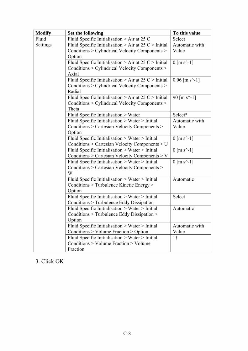
C-8
Modify Set the following To this value Fluid Settings
Fluid Specific Initialisation > Air at 25 C Select Fluid Specific Initialisation > Air at 25 C > Initial Conditions > Cylindrical Velocity Components > Option
Automatic with Value
Fluid Specific Initialisation > Air at 25 C > Initial Conditions > Cylindrical Velocity Components > Axial
0 [m s^-1]
Fluid Specific Initialisation > Air at 25 C > Initial Conditions > Cylindrical Velocity Components > Radial
0.06 [m s^-1]
Fluid Specific Initialisation > Air at 25 C > Initial Conditions > Cylindrical Velocity Components > Theta
90 [m s^-1]
Fluid Specific Initialisation > Water Select* Fluid Specific Initialisation > Water > Initial Conditions > Cartesian Velocity Components > Option
Automatic with Value
Fluid Specific Initialisation > Water > Initial Conditions > Cartesian Velocity Components > U
0 [m s^-1]
Fluid Specific Initialisation > Water > Initial Conditions > Cartesian Velocity Components > V
0 [m s^-1]
Fluid Specific Initialisation > Water > Initial Conditions > Cartesian Velocity Components > W
0 [m s^-1]
Fluid Specific Initialisation > Water > Initial Conditions > Turbulence Kinetic Energy > Option
Automatic
Fluid Specific Initialisation > Water > Initial Conditions > Turbulence Eddy Dissipation
Select
Fluid Specific Initialisation > Water > Initial Conditions > Turbulence Eddy Dissipation > Option
Automatic
Fluid Specific Initialisation > Water > Initial Conditions > Volume Fraction > Option
Automatic with Value
Fluid Specific Initialisation > Water > Initial Conditions > Volume Fraction > Volume Fraction
1†
3. Click OK
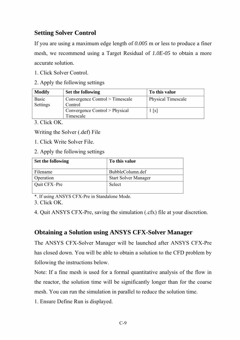
C-9
Setting Solver Control If you are using a maximum edge length of 0.005 m or less to produce a finer
mesh, we recommend using a Target Residual of 1.0E-05 to obtain a more
accurate solution.
1. Click Solver Control.
2. Apply the following settings Modify Set the following To this value Basic Settings
Convergence Control > Timescale Control
Physical Timescale
Convergence Control > Physical Timescale
1 [s]
3. Click OK.
Writing the Solver (.def) File
1. Click Write Solver File.
2. Apply the following settings Set the following To this value
Filename BubbleColumn.def Operation Start Solver Manager Quit CFX–Pre Select
*. If using ANSYS CFX-Pre in Standalone Mode. 3. Click OK.
4. Quit ANSYS CFX-Pre, saving the simulation (.cfx) file at your discretion.
Obtaining a Solution using ANSYS CFX-Solver Manager The ANSYS CFX-Solver Manager will be launched after ANSYS CFX-Pre
has closed down. You will be able to obtain a solution to the CFD problem by
following the instructions below.
Note: If a fine mesh is used for a formal quantitative analysis of the flow in
the reactor, the solution time will be significantly longer than for the coarse
mesh. You can run the simulation in parallel to reduce the solution time.
1. Ensure Define Run is displayed.
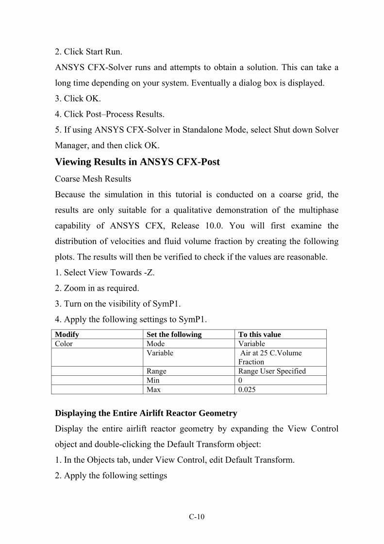
C-10
2. Click Start Run.
ANSYS CFX-Solver runs and attempts to obtain a solution. This can take a
long time depending on your system. Eventually a dialog box is displayed.
3. Click OK.
4. Click Post–Process Results.
5. If using ANSYS CFX-Solver in Standalone Mode, select Shut down Solver
Manager, and then click OK.
Viewing Results in ANSYS CFX-Post Coarse Mesh Results
Because the simulation in this tutorial is conducted on a coarse grid, the
results are only suitable for a qualitative demonstration of the multiphase
capability of ANSYS CFX, Release 10.0. You will first examine the
distribution of velocities and fluid volume fraction by creating the following
plots. The results will then be verified to check if the values are reasonable.
1. Select View Towards -Z.
2. Zoom in as required.
3. Turn on the visibility of SymP1.
4. Apply the following settings to SymP1. Modify Set the following To this value Color Mode Variable Variable Air at 25 C.Volume
Fraction Range Range User Specified Min 0 Max 0.025
Displaying the Entire Airlift Reactor Geometry
Display the entire airlift reactor geometry by expanding the View Control
object and double-clicking the Default Transform object:
1. In the Objects tab, under View Control, edit Default Transform.
2. Apply the following settings
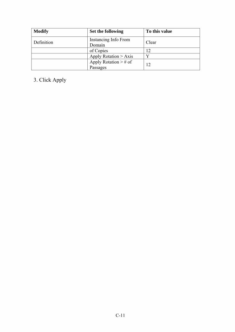
C-11
Modify Set the following To this value
Definition Instancing Info From Domain Clear
of Copies 12 Apply Rotation > Axis Y
Apply Rotation > # of Passages 12
3. Click Apply

C-12

وانا انهي بحثي ال .البحثهذا اشكر اهللا عز وجل الذي وفقني الآمال متطلبات ةفي البداي
ور نصيرعبود واالمتنان لالستاذ المشرف الدآتيسعني واعترافا بالفضل اال ان اتقدم بوافر الشكر
ترتب على لمواصلته ومتابعته العلمية للبحث وماموضوع الرسالة واشرافه عليها والقتراحه الحبوبى
.ذلك من توجيهات قيمه واراء سديدة
آما اتقدم بجزيل الشكر الى رئيس قسم الهندسة الكيمياوية، و جميع اساتذة قسم الهندسة
.ولمدهم يد العون لي خالل اعداد هذه الرسالةلمساعدتهم القيمة لي طيلة فترة الدراسة الكيمياوية
ودعمهم الدائم لي م،لمساعدتهآلية الهندسة /كري وامتناني الى عمادة جامعة النهرينبشواتقدم
.طيلة فترة الدراسة
وشكري الجزيل الى جميع زمالئي و زميالتي الذين مدو يد العون عند حاجتي اليها في
.البحث
بات وال انسى ان اتقدم بجزيل الشكر والتقدير الى من ساندني وساعدني على تخطي الصعو
.أخوتي وأخواتي ،العزيزة أمي خالل فترة البحث الى الذين ال مثيل لهم في الدنيا الى

الخالصةل اة تتعام ابية ةديناميكيمحاآ وائل الحس ادالت ) CFD(الس ل المع ع ح ةم ى الدينامكي ائلة عل الس
ة يتطلب نسبيا بضع فرضيات تق هذاواإللكترونية، الحواسيب ة ي لهيدروناميك اتام اعطي وصف تو ديري
. السائل قيقة لسلوكيعطى صورة د، ن التنبؤ التفصيلى للجريانأ .الفقاعية أألعمدة
وذج ANSYS باستخدام األبعادثالثية ) CFD(السوائل الحسابية ةديناميكيتم استخدام محاآاة مع نم
Euler-Euler ا من أنبوب يلقياس هايدروديناميكية العمود الفقاعي ذ السحب ، ومقارنتها مع مثيالته
ة اتن التجارب العملي الم ب ا الع ا و,) 1999(واخرين -التى اجراه ل أيضا مقارنته ة مفاع بهيدروناميكي
ود الفقاع واء ةعم ام ه تغل بنظ انس / ، يش ة المتج دفق الفقاع ام ت ي نظ اء ف وحظ. م رع دوران أن ل س
وهذاعمود الفقاعي، لل مثيالتها مع تهامقارنعند السحب أنبوب ىالسائل متجانسة في العمود الفقاعي ذ
الغاز و السائل تكون حرآةعمود الفقاعي للالسحب أنبوبفى . يؤدي إلى انخفاض معامل احتجاز الغاز
ي ع، بينما في العمود الفقاعي، تتوزالكتليتدفق ال ضمن نطاقعمليا سرعة الغاز و السائل بشكل قطع
.مكافئ
وب العمود الفقاعي ذي في مفاعالت لوحظ ال نظام ظهور السحب أنب از السطحية في سرع االنتق الغ
.في نظام تدفق الفقاعة المتجانس حتى سرع غاز سطحية أعلى بكثير لالشتغالالعالية بسبب قدرتها
باستخدام الفقاعيعمود الفي أطوار الجريانحساب
السوائل الحسابية ةديناميكي
رسالة
نهرينالفي جامعة هندسةمقدمة إلى كلية ال
ماجستير علوموهي جزء من متطلبات نيل درجة
الهندسة الكيمياويةفي
من قبل
رنا رسول جليل )2005في الهندسة الكيمياوية علوم بكالوريوس(
1430 محرم
2009 كانون الثاني