determination of potential of natural springs for water supply schemes

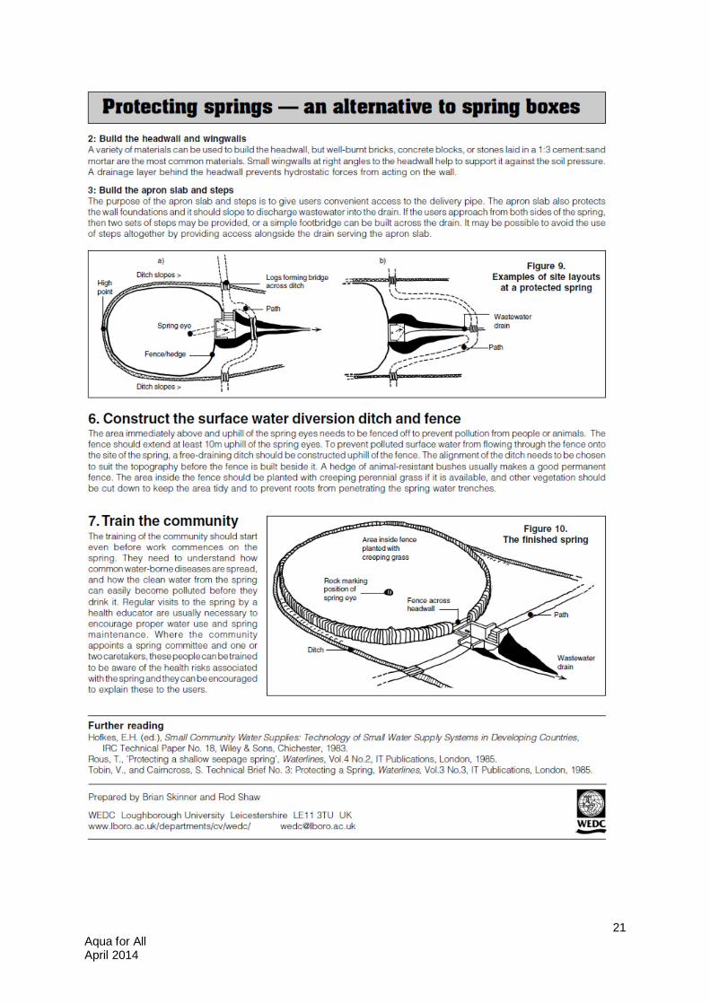
AquaShareware

Dick Bouman, April 2014

Determination of potential of natural springs for water supply schemes

Aqua for All Koningskade 40 2596 AA Den Haag P.O.Box 93218 2509 AE Den Haag +31 (0) 70 351 725 www.aquaforall.nl [email protected]

KvK 27248417 IBAN NL81 RABO 038384584

2 Aqua for All April 2014

Aqua for All is a Dutch organization, aiming to mobilize expertise and resources from the Dutch private sector to contribute to reaching the 7th Millennium Development Goal on water and sanitation. AquaShareware products are open source support materials for the water and sanitation sector and may be used free of charge, but with reference to Aqua for All. Any suggestion for correction, addition or remark is welcome at [email protected]. The author of this AquaShareware product, Mr. Dick Bouman, is head of the program desk and experienced in water resources and water supply. Mr. Dick Bouman started his career in 1981 with a water resource mapping in the Morogoro Region for DHV Consultants (now Royal Haskoning DHV), with emphasis on low flow analysis of small streams.


Contents 1. Introduction.........................................................................................................................4 2. Spring types .......................................................................................................................5 3. Yield measurements ...........................................................................................................6 4. Depletion theory .................................................................................................................8 5. A short introduction to statistics ........................................................................................10 6. Methods to determine the once in 20 years minimum flow ................................................12

6.1 Extrapolation method ..................................................................................................12 6.2 Correlation method ......................................................................................................14

7. Design Spring Protection ..................................................................................................17 Attachment: Protecting Springs ............................................................................................18


1. Introduction For a good water supply design, one should be sure about the capacity of the source, for which the minimum yield is a critical factor. The standard for rural design is that only once in 20 years, the minimum flow at the source may drop below the design flow of the water supply system, which is mostly related to the population in 20 years’ time. Aqua for All gets many applications for spring based water systems, but rarely there is more than one random discharge measurement, somewhere in the dry season, without indication of reliability. Gravity based water schemes that suffer from seasonal or permanent shortages are a source of conflict, and require a lot of skills and effort of the scheme attendant. Therefore it is a precondition for design that the capacity of the source is determined. This instruction is limited to springs. For streams, the theory is comparable, but often more complex. Apart from minimum flows, other aspects are relevant, but not fully dealt with in this manual:

water quality (pathogens, turbidity, iron, fluoride, other salts), excessive rainfall, erosion and risk of inflow of polluted storm drainage water design of spring captures legal and institutional aspects, especially in case of multiple use catchment protection to avoid a further depletion of spring flows

Literature can be found at http://www.akvo.org/wiki/index.php/Springwater_collection , where also reference is made to other literature. Step A It is important to make an initial reconnaissance of all water resources in the area and to evaluate their potential (and risks) for all possible users and use types. This can best be done with the community, starting with a participative mapping exercise and a check on maps and satellite images (e.g. through Google Earth). Understanding the ‘natural water system’ is a very important input for further analysis. The best is to work within the natural water catchment in which the community is located, bordered by water divides. A very helpful mapping tool can be found at http://www.samsamwater.com/catchments/ , in which the water divide can be drawn in Google Earth. This website contains also other mapping tools, which can be used in combination with Google Earth (http://www.samsamwater.com/tools.php). A reconnaissance should investigate for each water source the location/altitude, type, size, permanence of flow, yield (especially at end of dry season), water quality (seasonal fluctuations), risks of damage or pollution, present and potential use, present ownership, ecological value etc. This manual is focused on springs, but most of the information can also be used for streams. Separate AquaShareware is developed to determine other run off characteristics (Run off determination) and for hydraulic design for gravity schemes. A separate publication on institutional models is under preparation.


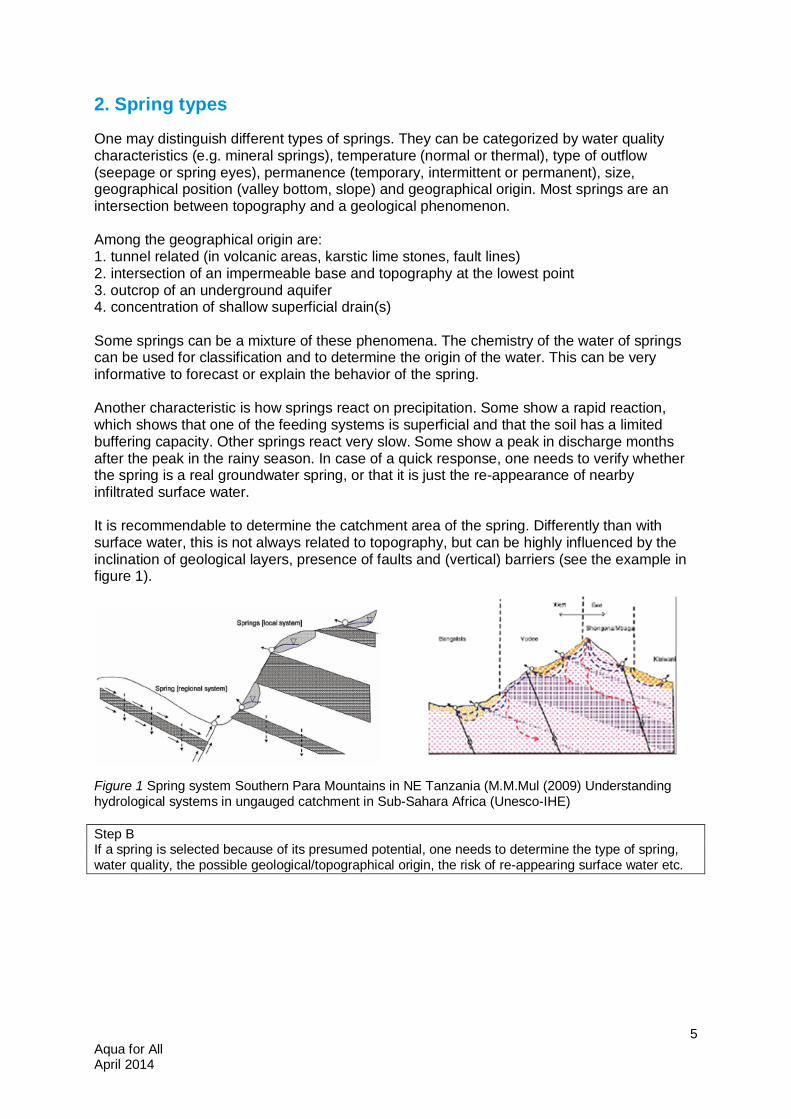
2. Spring types One may distinguish different types of springs. They can be categorized by water quality characteristics (e.g. mineral springs), temperature (normal or thermal), type of outflow (seepage or spring eyes), permanence (temporary, intermittent or permanent), size, geographical position (valley bottom, slope) and geographical origin. Most springs are an intersection between topography and a geological phenomenon. Among the geographical origin are: 1. tunnel related (in volcanic areas, karstic lime stones, fault lines) 2. intersection of an impermeable base and topography at the lowest point 3. outcrop of an underground aquifer 4. concentration of shallow superficial drain(s) Some springs can be a mixture of these phenomena. The chemistry of the water of springs can be used for classification and to determine the origin of the water. This can be very informative to forecast or explain the behavior of the spring. Another characteristic is how springs react on precipitation. Some show a rapid reaction, which shows that one of the feeding systems is superficial and that the soil has a limited buffering capacity. Other springs react very slow. Some show a peak in discharge months after the peak in the rainy season. In case of a quick response, one needs to verify whether the spring is a real groundwater spring, or that it is just the re-appearance of nearby infiltrated surface water. It is recommendable to determine the catchment area of the spring. Differently than with surface water, this is not always related to topography, but can be highly influenced by the inclination of geological layers, presence of faults and (vertical) barriers (see the example in figure 1).

Figure 1 Spring system Southern Para Mountains in NE Tanzania (M.M.Mul (2009) Understanding hydrological systems in ungauged catchment in Sub-Sahara Africa (Unesco-IHE) Step B If a spring is selected because of its presumed potential, one needs to determine the type of spring, water quality, the possible geological/topographical origin, the risk of re-appearing surface water etc.


3. Yield measurements Yield or discharges are expressed as volume per unit of time (l/s, m3/s, m3/hr, m3/day). 1 l/s = 3.6 m3/hr = 86.4 m3/day. The ‘specific yield’ is the yield per area unit (yield divided by catchment area), mostly expressed as l/s/km2. This specific yield is often seen as a characteristic of a wider area with similar geographic conditions (precipitation, soil, morphology and geology). The measurement of spring discharges can be done with different methods:

1. bucket/stopwatch. Try to concentrate the flow in one channel/drain and collect it in a bucket or container. The volume of the bucket divided by the filling time is the discharge. You might apply a correction factor if you cannot concentrate the entire flow. Repeat the measurement several times and calculate the average, excluding the extremes. Preferably, the ‘constructions that were made for easier measurement’ should remain, to facilitate later measurement and to improve the comparability.

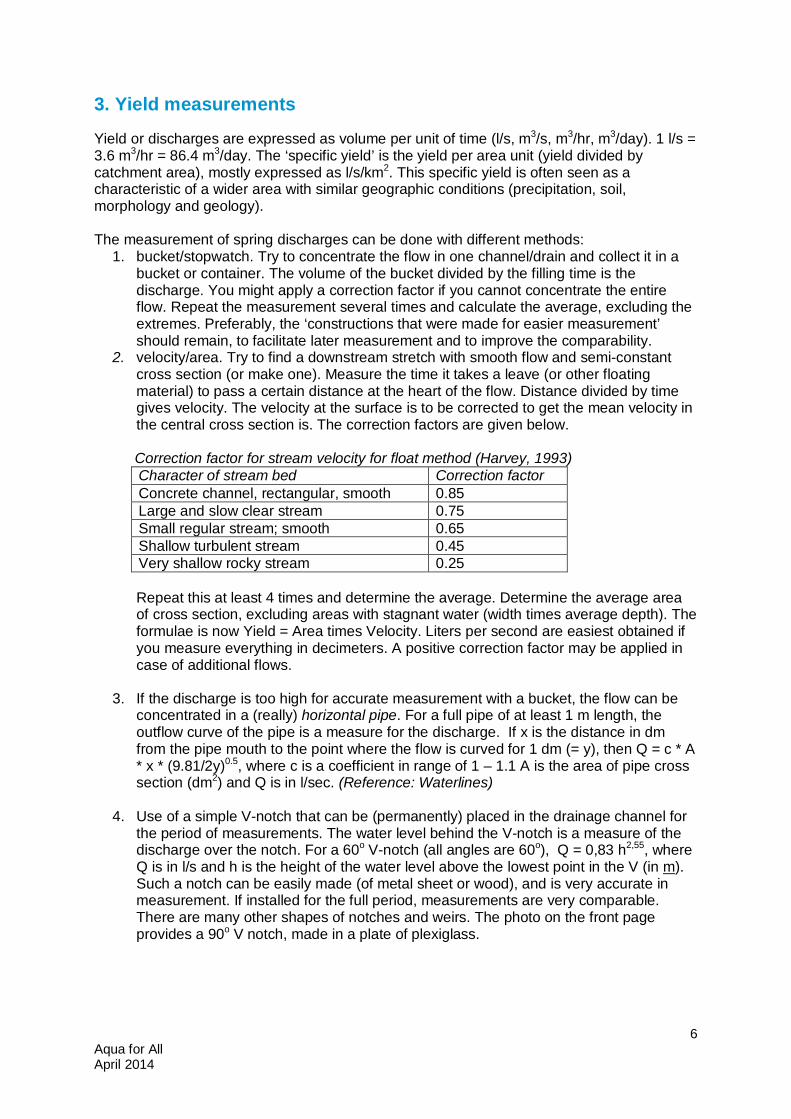
2. velocity/area. Try to find a downstream stretch with smooth flow and semi-constant cross section (or make one). Measure the time it takes a leave (or other floating material) to pass a certain distance at the heart of the flow. Distance divided by time gives velocity. The velocity at the surface is to be corrected to get the mean velocity in the central cross section is. The correction factors are given below.

Correction factor for stream velocity for float method (Harvey, 1993)

Character of stream bed Correction factor Concrete channel, rectangular, smooth 0.85 Large and slow clear stream 0.75 Small regular stream; smooth 0.65 Shallow turbulent stream 0.45 Very shallow rocky stream 0.25

Repeat this at least 4 times and determine the average. Determine the average area of cross section, excluding areas with stagnant water (width times average depth). The formulae is now Yield = Area times Velocity. Liters per second are easiest obtained if you measure everything in decimeters. A positive correction factor may be applied in case of additional flows.

3. If the discharge is too high for accurate measurement with a bucket, the flow can be

concentrated in a (really) horizontal pipe. For a full pipe of at least 1 m length, the outflow curve of the pipe is a measure for the discharge. If x is the distance in dm from the pipe mouth to the point where the flow is curved for 1 dm (= y), then Q = c * A * x * (9.81/2y)0.5, where c is a coefficient in range of 1 – 1.1 A is the area of pipe cross section (dm2) and Q is in l/sec. (Reference: Waterlines)

4. Use of a simple V-notch that can be (permanently) placed in the drainage channel for

the period of measurements. The water level behind the V-notch is a measure of the discharge over the notch. For a 60o V-notch (all angles are 60o), Q = 0,83 h2,55, where Q is in l/s and h is the height of the water level above the lowest point in the V (in m). Such a notch can be easily made (of metal sheet or wood), and is very accurate in measurement. If installed for the full period, measurements are very comparable. There are many other shapes of notches and weirs. The photo on the front page provides a 90o V notch, made in a plate of plexiglass.


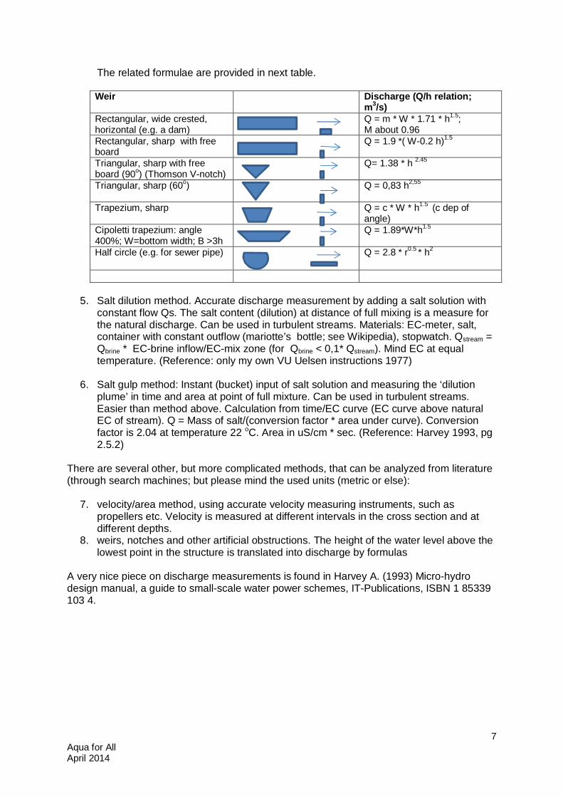
The related formulae are provided in next table. Weir Discharge (Q/h relation;

m3/s) Rectangular, wide crested, horizontal (e.g. a dam)

Q = m * W * 1.71 * h1.5; M about 0.96

Rectangular, sharp with free board

Q = 1.9 *( W-0.2 h)1.5

Triangular, sharp with free board (90o) (Thomson V-notch)

Q= 1.38 * h 2.45

Triangular, sharp (60o)

Q = 0,83 h2,55

Trapezium, sharp Q = c * W * h1.5 (c dep of angle)

Cipoletti trapezium: angle 400%; W=bottom width; B >3h

Q = 1.89*W*h1.5

Half circle (e.g. for sewer pipe)

Q = 2.8 * r0.5 * h2

5. Salt dilution method. Accurate discharge measurement by adding a salt solution with constant flow Qs. The salt content (dilution) at distance of full mixing is a measure for the natural discharge. Can be used in turbulent streams. Materials: EC-meter, salt, container with constant outflow (mariotte’s bottle; see Wikipedia), stopwatch. Qstream = Qbrine * EC-brine inflow/EC-mix zone (for Qbrine < 0,1* Qstream). Mind EC at equal temperature. (Reference: only my own VU Uelsen instructions 1977)

6. Salt gulp method: Instant (bucket) input of salt solution and measuring the ‘dilution

plume’ in time and area at point of full mixture. Can be used in turbulent streams. Easier than method above. Calculation from time/EC curve (EC curve above natural EC of stream). Q = Mass of salt/(conversion factor * area under curve). Conversion factor is 2.04 at temperature 22 oC. Area in uS/cm * sec. (Reference: Harvey 1993, pg 2.5.2)

There are several other, but more complicated methods, that can be analyzed from literature (through search machines; but please mind the used units (metric or else):

7. velocity/area method, using accurate velocity measuring instruments, such as propellers etc. Velocity is measured at different intervals in the cross section and at different depths.

8. weirs, notches and other artificial obstructions. The height of the water level above the lowest point in the structure is translated into discharge by formulas

A very nice piece on discharge measurements is found in Harvey A. (1993) Micro-hydro design manual, a guide to small-scale water power schemes, IT-Publications, ISBN 1 85339 103 4.


4. Depletion theory The most common depletion of a spring follows an inverse logarithmic equation: Qt1 = Qt0 x e-

a x(t1-t0) This formulae shows the yield (Q) at a certain time (t1) in relation to the yield at an earlier date during the same dry period (Qt0). Q is mostly expressed as l/sec or m3/s. This behaviour is comparable to the decline of the outflow through a bottom tap in a jerrycan (with open top), in which the lowering water table has less and less pressure on the water at the outflow point.

When plotted on semi-log paper (Q on y-axis as elog, time on x-axis as linear), the depletion follows a straight downward line. Time is mostly expressed in days. The value of ‘e’ is 2.718 (the ‘natural logarithmic’). The variable ‘a’ is the reservoir depletion coefficient (1/day). The inverse of ‘a’ (1/a; in days) is a very helpful variable. The period in which the flow is divided by two is 0.65 x 1/a. And the total water volume, stored in the reservoir behind the spring at a certain time is Q/a (if Q is expressed in m3/d and a in 1/day; the stored volume is in m3). If one knows the area of the feeding catchment (km2), one can translate the volume (m3) to m3/km2 or 10-3 mm. In the latter form it is easy to relate to the precipitation. Not all the springs show this straight line. The most common deviation is that it becomes less inclined with time, often with a clear deflection-point. In such a case, the spring might be supplied from 2 hydrologic reservoirs: one with a rapid depletion and one with a slower depletion. The deflection point is where the reservoir with rapid depletion has become (almost) empty. This may happen with a spring, fed by a superficial soil related reservoir and a deeper (confined) groundwater reservoir. Also the lower outlet in the lowest reservoir of figure 2 would show such a concave decline. A concave shape can also originate from a situation, where part of the recharge comes from a surface reservoir in the catchment area or leaking permanent streams, or from deep confined reservoirs (such as in the valley well in the left section of figure 1).

y = 8,064e-0,02x0,14

0,37

1,00

2,70

7,29

19,68

0 50 100 150 200

Q (l/s)Q (l/s)

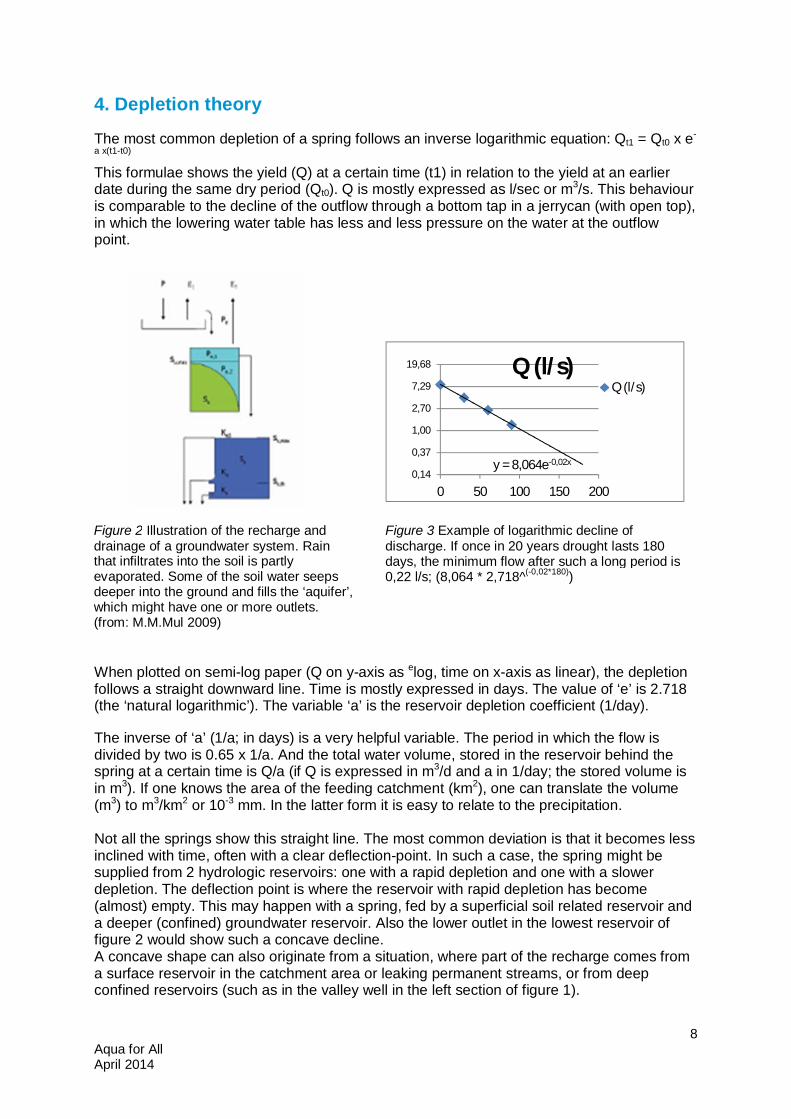
Figure 2 Illustration of the recharge and drainage of a groundwater system. Rain that infiltrates into the soil is partly evaporated. Some of the soil water seeps deeper into the ground and fills the ‘aquifer’, which might have one or more outlets. (from: M.M.Mul 2009)

Figure 3 Example of logarithmic decline of discharge. If once in 20 years drought lasts 180 days, the minimum flow after such a long period is 0,22 l/s; (8,064 * 2,718^(-0,02*180))


The inverse shape (convex with a down going tail) is rather common. This can originate from different situations:

1. The spring is fed from or located in a swampy area, which dries up in the dry season. 2. The spring is just one of the (higher) outflows of a larger underground reservoir.

Outflows at lower altitude may continue; whereas the upper spring dries due to a (rapidly) declining water table. The middle outlet in the lower reservoir of figure 2 is such an example.

There are exceptional situations, where springs show patterns that differ from the depletion theory, described above. In limestone and volcanic areas, spring discharges may show (extreme) oscillations, due to natural ‘siphon’ systems in the underground ‘tunnels’. In areas with snow or glaciers, the melting may give daily fluctuations. It is recommended to inquire the nearby community or land owners on the specific characteristics of the spring. This is valuable, but remember that most memories are rather biased when it relates to weather and other natural phenomena, for which it is common to deviate from the average.


5. A short introduction to statistics When we have a series of rainfall data or minimum yields or lengths of drought, we can determine the average. The average is the sum of all data, divided by the number of data. This can be different from the median. The median is the value between the 50% lowest data and the 50% highest data. For the purpose of this instruction, the ‘distribution’ of data is very relevant. The distribution is the division of the number of data per interval/range. The most common distribution is the ‘normal distribution’, in which the data are symmetrically distributed around the average and in which the probability that a value is higher becomes lower in function of the difference with the average.

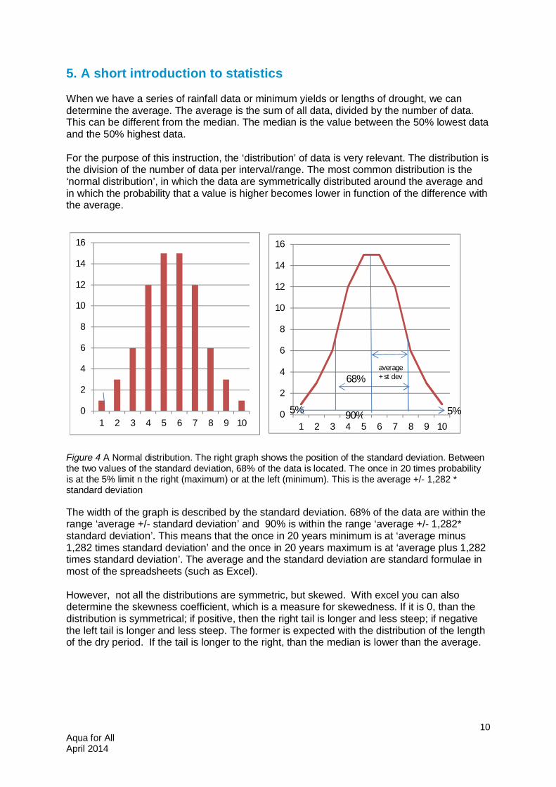
Figure 4 A Normal distribution. The right graph shows the position of the standard deviation. Between the two values of the standard deviation, 68% of the data is located. The once in 20 times probability is at the 5% limit n the right (maximum) or at the left (minimum). This is the average +/- 1,282 * standard deviation The width of the graph is described by the standard deviation. 68% of the data are within the range ‘average +/- standard deviation’ and 90% is within the range ‘average +/- 1,282* standard deviation’. This means that the once in 20 years minimum is at ‘average minus 1,282 times standard deviation’ and the once in 20 years maximum is at ‘average plus 1,282 times standard deviation’. The average and the standard deviation are standard formulae in most of the spreadsheets (such as Excel). However, not all the distributions are symmetric, but skewed. With excel you can also determine the skewness coefficient, which is a measure for skewedness. If it is 0, than the distribution is symmetrical; if positive, then the right tail is longer and less steep; if negative the left tail is longer and less steep. The former is expected with the distribution of the length of the dry period. If the tail is longer to the right, than the median is lower than the average.

0

2

4

6

8

10

12

14

16

1 2 3 4 5 6 7 8 9 100

2

4

6

8

10

12

14

16

1 2 3 4 5 6 7 8 9 10

average+ st dev68%

5%5% 90%


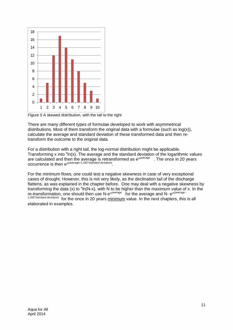
Figure 5 A skewed distribution, with the tail to the right There are many different types of formulae developed to work with asymmetrical distributions. Most of them transform the original data with a formulae (such as log(x)), calculate the average and standard deviation of these transformed data and then re-transform the outcome to the original data. For a distribution with a right tail, the log-normal distribution might be applicable. Transforming x into eln(x). The average and the standard deviation of the logarithmic values are calculated and then the average is retransformed as e^average . The once in 20 years occurrence is then e^(average+1,282*standard deviation). For the minimum flows, one could test a negative skewness in case of very exceptional cases of drought. However, this is not very likely, as the declination tail of the discharge flattens, as was explained in the chapter before. One may deal with a negative skewness by transforming the data (x) to eln(N-x), with N to be higher than the maximum value of x. In the re-transformation, one should then use N-e^average for the average and N- e^(average -

1,282*standard deviation) for the once in 20 years minimum value. In the next chapters, this is all elaborated in examples.

0

2

4

6

8

10

12

14

16

18

1 2 3 4 5 6 7 8 9 10


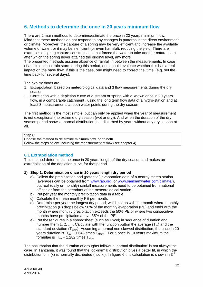
6. Methods to determine the once in 20 years minimum flow There are 2 main methods to determine/estimate the once in 20 years minimum flow. Mind that these methods do not respond to any changes in patterns in the direct environment or climate. Moreover, the capture of a spring may be very efficient and increase the available volume of water, or it may be inefficient (or even harmful), reducing the yield. There are examples of spring capture constructions, that forced the water to take another natural path, after which the spring never attained the original level, any more. The presented methods assume absence of rainfall in between the measurements. In case of an exceptional rain storm during this period, one should evaluate whether this has a real impact on the base flow. If this is the case, one might need to correct the ‘time’ (e.g. set the time back for several days). The two methods are: 1. Extrapolation, based on meteorological data and 3 flow measurements during the dry

season 2. Correlation with a depletion curve of a stream or spring with a known once in 20 years

flow, in a comparable catchment , using the long term flow data of a hydro-station and at least 3 measurements at both water points during the dry season

The first method is the most simple, but can only be applied when the year of measurement is not exceptional (no extreme dry season (wet or dry)). And when the duration of the dry season period shows a normal distribution; not disturbed by years without any dry season at all. Step C Choose the method to determine minimum flow, or do both Follow the steps below, including the measurement of flow (see chapter 4)

6.1 Extrapolation method This method determines the once in 20 years length of the dry season and makes an extrapolation of the depletion curve for that period. 1) Step 1: Determination once in 20 years length dry period

a) Collect the precipitation and (potential) evaporation data of a nearby meteo station (averages can be obtained from www.fao.org, or www.samsamwater.com/climate/), but real (daily or monthly) rainfall measurements need to be obtained from national offices or from the attendant of the meteorological station.

b) Put per year the monthly precipitation data in a table. c) Calculate the mean monthly PE per month. d) Determine per year the longest dry period, which starts with the month where monthly

precipitation (P) drops below 50% of the monthly evaporation (PE) and ends with the month where monthly precipitation exceeds the 50% PE or where two consecutive months have precipitation above 35% of the PE.

e) Put these figures in a spreadsheet (such as Excel) in sequence of duration and number them 1, 2, … . Calculate with the function button the average (Tav) and the standard deviation (Tstdev). Assuming a normal non skewed distribution, the once in 20 years duration is Tav + 1.645 times Tstdev. For a once in 10 years maximum the formulae is Tav + 1.282 times Tstdev

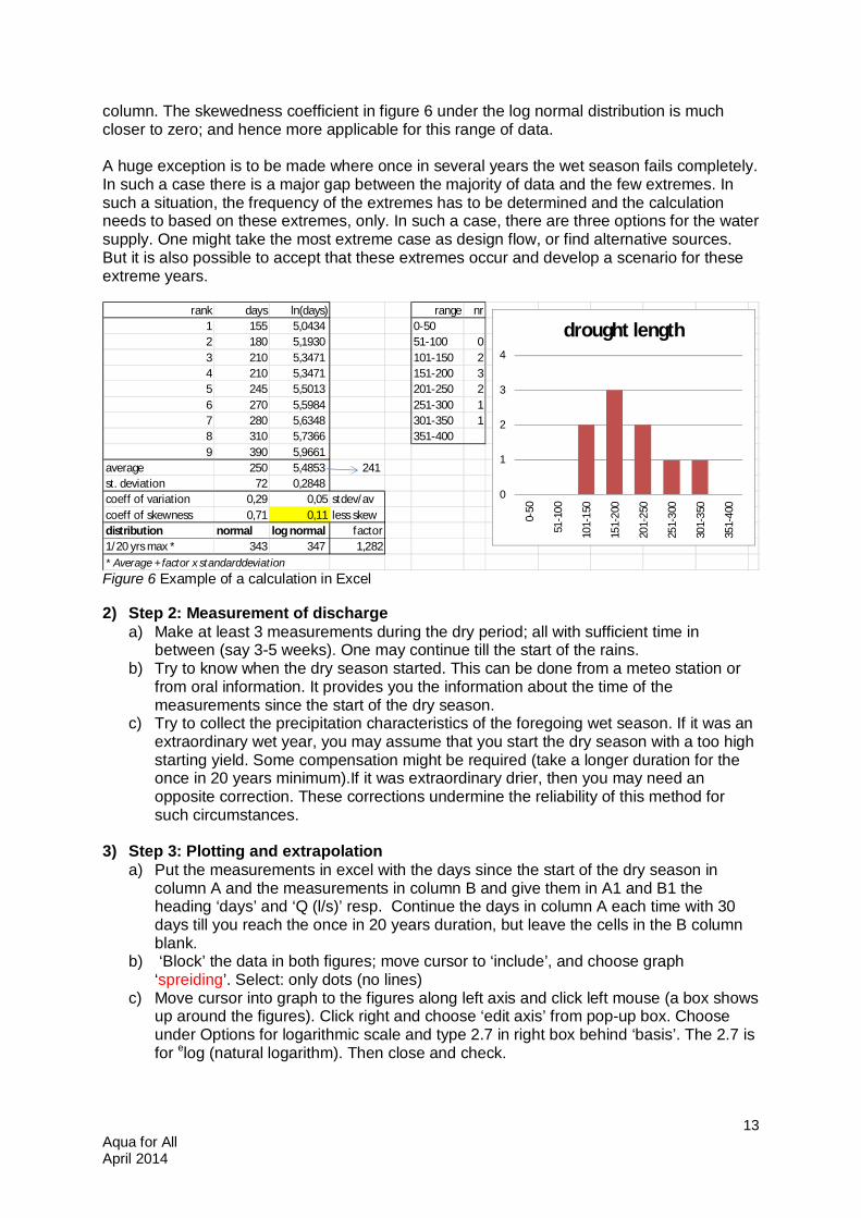
The assumption that the duration of droughts follows a ‘normal distribution’ is not always the case. In Tanzania, it was found that the log-normal distribution gives a better fit, in which the distribution of ln(x) is normally distributed (not ‘x’). In figure 6 this calculation is shown in 3rd


column. The skewedness coefficient in figure 6 under the log normal distribution is much closer to zero; and hence more applicable for this range of data. A huge exception is to be made where once in several years the wet season fails completely. In such a case there is a major gap between the majority of data and the few extremes. In such a situation, the frequency of the extremes has to be determined and the calculation needs to based on these extremes, only. In such a case, there are three options for the water supply. One might take the most extreme case as design flow, or find alternative sources. But it is also possible to accept that these extremes occur and develop a scenario for these extreme years.

Figure 6 Example of a calculation in Excel 2) Step 2: Measurement of discharge

a) Make at least 3 measurements during the dry period; all with sufficient time in between (say 3-5 weeks). One may continue till the start of the rains.

b) Try to know when the dry season started. This can be done from a meteo station or from oral information. It provides you the information about the time of the measurements since the start of the dry season.

c) Try to collect the precipitation characteristics of the foregoing wet season. If it was an extraordinary wet year, you may assume that you start the dry season with a too high starting yield. Some compensation might be required (take a longer duration for the once in 20 years minimum).If it was extraordinary drier, then you may need an opposite correction. These corrections undermine the reliability of this method for such circumstances.

3) Step 3: Plotting and extrapolation

a) Put the measurements in excel with the days since the start of the dry season in column A and the measurements in column B and give them in A1 and B1 the heading ‘days’ and ‘Q (l/s)’ resp. Continue the days in column A each time with 30 days till you reach the once in 20 years duration, but leave the cells in the B column blank.

b) ‘Block’ the data in both figures; move cursor to ‘include’, and choose graph ‘spreiding’. Select: only dots (no lines)

c) Move cursor into graph to the figures along left axis and click left mouse (a box shows up around the figures). Click right and choose ‘edit axis’ from pop-up box. Choose under Options for logarithmic scale and type 2.7 in right box behind ‘basis’. The 2.7 is for elog (natural logarithm). Then close and check.

rank days ln(days) range nr1 155 5,0434 0-502 180 5,1930 51-100 03 210 5,3471 101-150 24 210 5,3471 151-200 35 245 5,5013 201-250 26 270 5,5984 251-300 17 280 5,6348 301-350 18 310 5,7366 351-4009 390 5,9661

average 250 5,4853 241 st. deviation 72 0,2848 coeff of variation 0,29 0,05 stdev/avcoeff of skewness 0,71 0,11 less skewdistribution normal log normal factor1/20 yrs max * 343 347 1,282* Average + factor x standarddeviation

0

1

2

3

4

0-50

51-1

00

101-

150

151-

200

201-

250

251-

300

301-

350

351-

400

drought length


d) Move cursor to one of the measurements and click left mouse (repeat till they show a blocked square around the dots). Then right mouse and choose ‘add trendline’; choose exponential (in top) and ‘show formulae’ at the bottom; OK/close.

e) Check whether the measurements do not deviate too much from the trendline (if you have more than 3 you might remove the one which deviates most in case you think the deviation is due to an error).

f) The formulae should show like: 8 * e (-0,02*x), in which 0.02 is the reservoir depletion coefficient.

g) Calculate the once in 20 years minimum flow with a drought length of 347 days: in the example 8,08 * 2,718^(-0,019*347) .

Figure 7 Example of an excel file to determine once in 20 years minimum (at 347 days) You might make a ‘mother’ file with the prepared graph and just renew the file with new data any time you need to make a new one. (rename the file).

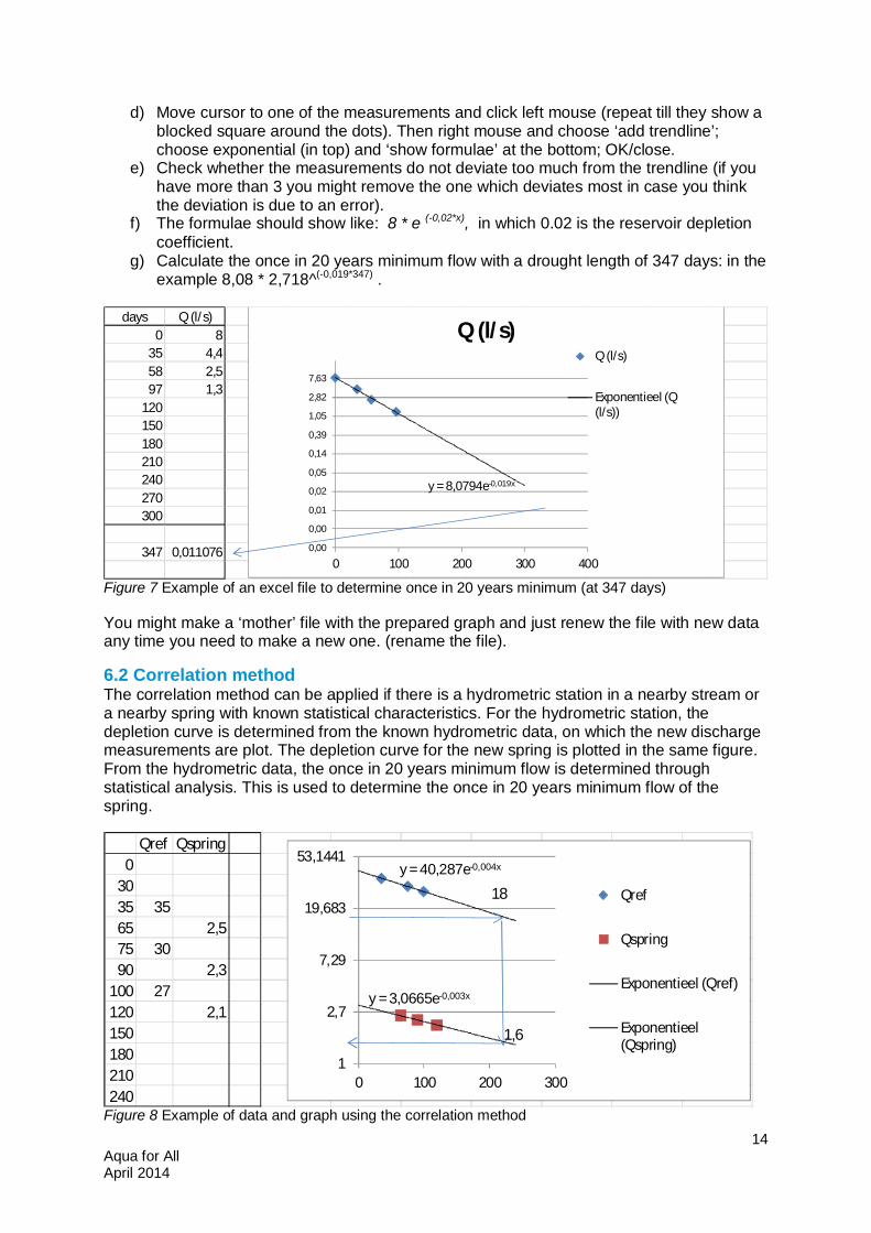
6.2 Correlation method The correlation method can be applied if there is a hydrometric station in a nearby stream or a nearby spring with known statistical characteristics. For the hydrometric station, the depletion curve is determined from the known hydrometric data, on which the new discharge measurements are plot. The depletion curve for the new spring is plotted in the same figure. From the hydrometric data, the once in 20 years minimum flow is determined through statistical analysis. This is used to determine the once in 20 years minimum flow of the spring.

Figure 8 Example of data and graph using the correlation method

days Q (l/s)0 8

35 4,458 2,597 1,3

120150180210240270300

347 0,011076

y = 8,0794e-0,019x

0,00

0,00

0,01

0,02

0,05

0,14

0,39

1,05

2,82

7,63

0 100 200 300 400

Q (l/s)Q (l/s)

Exponentieel (Q(l/s))

Qref Qspring0

3035 3565 2,575 3090 2,3

100 27120 2,1150180210240

y = 40,287e-0,004x

y = 3,0665e-0,003x

1

2,7

7,29

19,683

53,1441

0 100 200 300

Qref

Qspring

Exponentieel (Qref)

Exponentieel(Qspring)

18

1,6


Although the scale of the two water sources may be different, there might be similarities in recent precipitation history and reaction characteristics. This might overcome the problem of extremities during the past wet season or interruptions with storms during the dry season. 1) Step 1: Measurement of discharge at both water points

a) At each water point at least 3 measurements have to be taken at acceptable intervals (mostly >30 days). There is no need to do the measurements at the same date.

b) Make for both stations a graph such as is done in figure 6. For the graph of the hydrometric station, one may also make a (third) depletion graph from historical data.

2) Step 2: Determination the once in 20 minimum flow at hydrometric station

a) Take from the hydrometric station data the lowest minimum flow in each year. b) Put these figures in excel in sequence of duration and number them 1, 2, … .

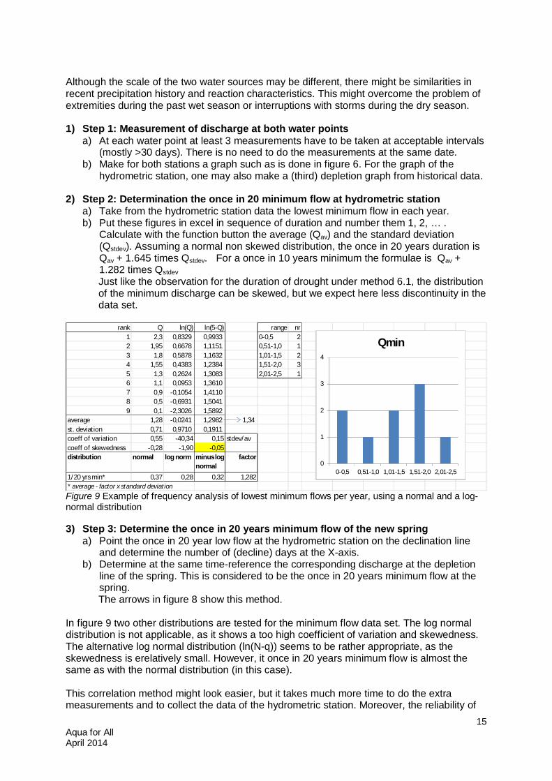
Calculate with the function button the average (Qav) and the standard deviation (Qstdev). Assuming a normal non skewed distribution, the once in 20 years duration is Qav + 1.645 times Qstdev. For a once in 10 years minimum the formulae is Qav + 1.282 times Qstdev Just like the observation for the duration of drought under method 6.1, the distribution of the minimum discharge can be skewed, but we expect here less discontinuity in the data set.

Figure 9 Example of frequency analysis of lowest minimum flows per year, using a normal and a log-normal distribution 3) Step 3: Determine the once in 20 years minimum flow of the new spring

a) Point the once in 20 year low flow at the hydrometric station on the declination line and determine the number of (decline) days at the X-axis.

b) Determine at the same time-reference the corresponding discharge at the depletion line of the spring. This is considered to be the once in 20 years minimum flow at the spring. The arrows in figure 8 show this method.

In figure 9 two other distributions are tested for the minimum flow data set. The log normal distribution is not applicable, as it shows a too high coefficient of variation and skewedness. The alternative log normal distribution (ln(N-q)) seems to be rather appropriate, as the skewedness is erelatively small. However, it once in 20 years minimum flow is almost the same as with the normal distribution (in this case). This correlation method might look easier, but it takes much more time to do the extra measurements and to collect the data of the hydrometric station. Moreover, the reliability of

rank Q ln(Q) ln(5-Q) range nr1 2,3 0,8329 0,9933 0-0,5 22 1,95 0,6678 1,1151 0,51-1,0 13 1,8 0,5878 1,1632 1,01-1,5 24 1,55 0,4383 1,2384 1,51-2,0 35 1,3 0,2624 1,3083 2,01-2,5 16 1,1 0,0953 1,3610 7 0,9 -0,1054 1,4110 8 0,5 -0,6931 1,5041 9 0,1 -2,3026 1,5892

average 1,28 -0,0241 1,2982 1,34 st. deviation 0,71 0,9710 0,1911 coeff of variation 0,55 -40,34 0,15 stdev/avcoeff of skewedness -0,28 -1,90 -0,05distribution normal log norm minus log

normalfactor

1/20 yrs min* 0,37 0,28 0,32 1,282* average - factor x standard deviation

0

1

2

3

4

0-0,5 0,51-1,0 1,01-1,5 1,51-2,0 2,01-2,5

Qmin


run off data is often much lower than rainfall data. The method is very useful if one makes an water resource analysis for a larger area. This method was successfully applied by the author (under contract of DHV) for the analysis of the potential of surface water resources for water supply in the Morogoro Region in Central Tanzania in 1981.


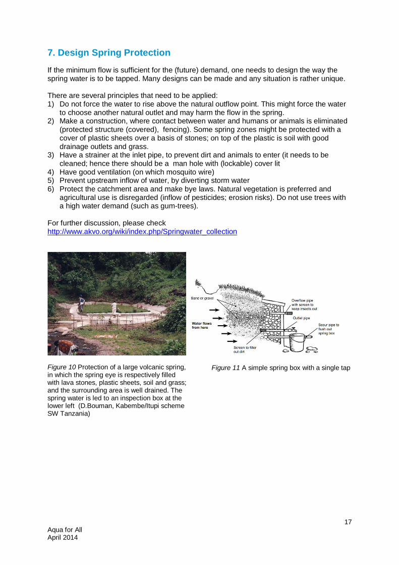
7. Design Spring Protection If the minimum flow is sufficient for the (future) demand, one needs to design the way the spring water is to be tapped. Many designs can be made and any situation is rather unique. There are several principles that need to be applied: 1) Do not force the water to rise above the natural outflow point. This might force the water

to choose another natural outlet and may harm the flow in the spring. 2) Make a construction, where contact between water and humans or animals is eliminated

(protected structure (covered), fencing). Some spring zones might be protected with a cover of plastic sheets over a basis of stones; on top of the plastic is soil with good drainage outlets and grass.

3) Have a strainer at the inlet pipe, to prevent dirt and animals to enter (it needs to be cleaned; hence there should be a man hole with (lockable) cover lit

4) Have good ventilation (on which mosquito wire) 5) Prevent upstream inflow of water, by diverting storm water 6) Protect the catchment area and make bye laws. Natural vegetation is preferred and

agricultural use is disregarded (inflow of pesticides; erosion risks). Do not use trees with a high water demand (such as gum-trees).

For further discussion, please check http://www.akvo.org/wiki/index.php/Springwater_collection

Figure 10 Protection of a large volcanic spring, in which the spring eye is respectively filled with lava stones, plastic sheets, soil and grass; and the surrounding area is well drained. The spring water is led to an inspection box at the lower left (D.Bouman, Kabembe/Itupi scheme SW Tanzania)

Figure 11 A simple spring box with a single tap


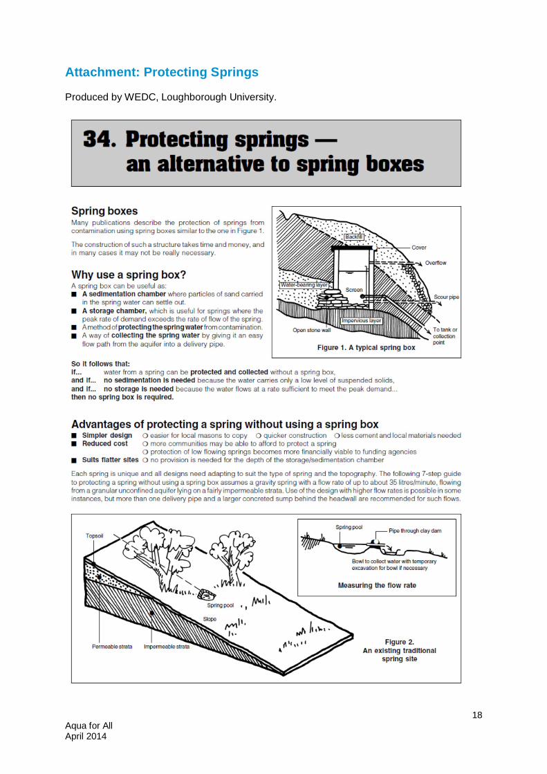
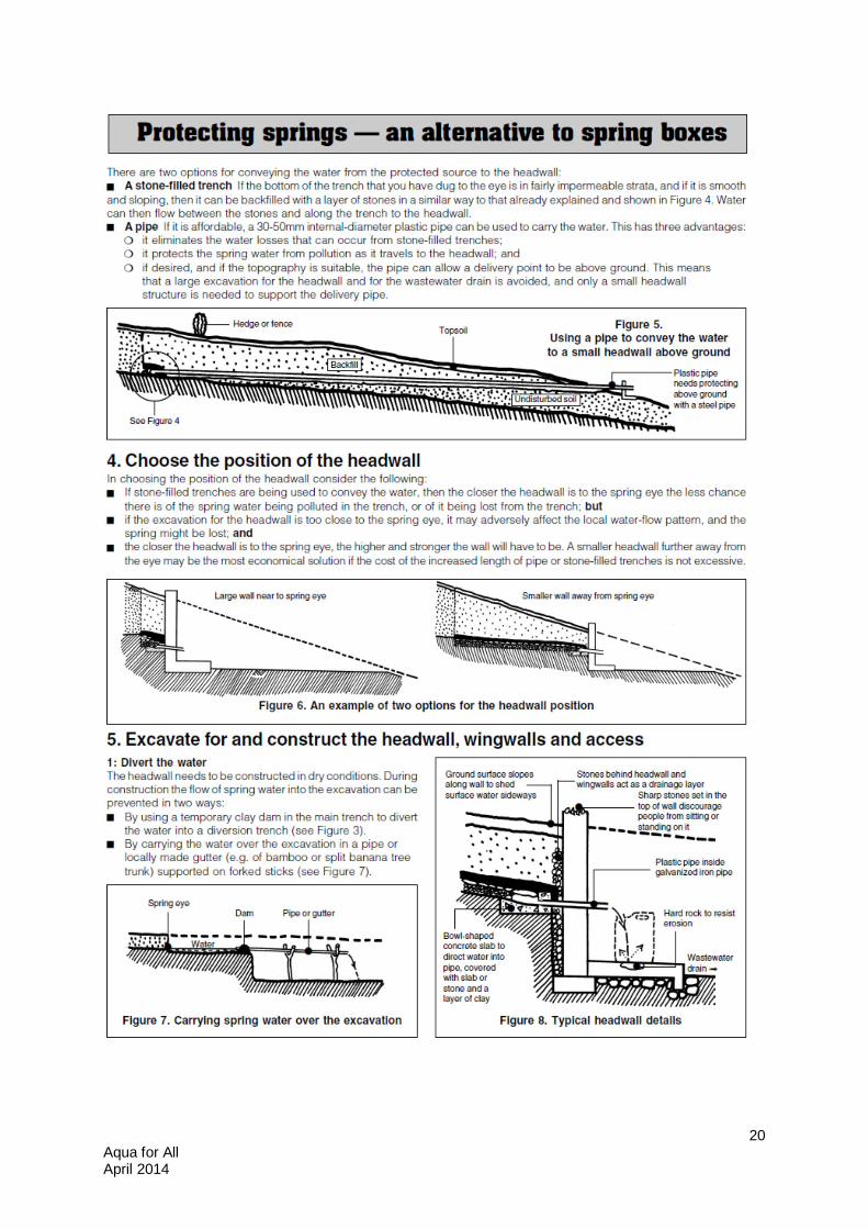
Attachment: Protecting Springs Produced by WEDC, Loughborough University.

determination of potential of natural springs for water supply schemes

Documents