FS-05-129-AKSIGMA ISSN 1013-4506

DETERMINATION OF THE DETECTION LIMIT AND DECISION THRESHOLD FOR IONIZING-RADIATION MEASUREMENTS: FUNDAMENTALS AND PARTICULAR APPLICATIONS Proposal for a standard

K. Weise K. Hübel

R. Michel E. Rose

M. Schläger D. Schrammel

M. Täschner

ISSN 1013-4506 ISBN 3-8249-0945-6 © by TÜV-Verlag GmbH, Köln TÜV Rheinland Group, Köln 2004 Gesamtherstellung: TÜV-Verlag GmbH, Köln Printed in Germany 2005

Prologue

The recognition and detection of ionizing radiation are indispensable basic prerequisites ofradiation protection. For this purpose, the standard series DIN 25482 and the correspondingstandard series ISO 11929 provide decision thresholds, detection limits, and confidence limitsfor a diversity of application fields. The decision threshold allows a decision to be made fora measurement on whether or not, for instance, radiation of a possibly radioactive sample ispresent. The detection limit allows a decision on whether or not the measurement procedureintended for application to the measurement meets the requirements to be fulfilled and istherefore appropriate for the measurement purpose. Confidence limits enclose with a specifiedprobability the true value of the measurand to be measured.

Because of recent developments in metrology concerning measurement uncertainty (DIN 1319and ISO Guide to the expression of uncertainty in measurement), the older Parts 1 to 7 (exceptPart 4) of DIN 25482 and the corresponding Parts 1 to 4 of ISO 11929 urgently need a revisionbased on the common, already laid statistical foundation of Part 10 of DIN 25482. The modernParts 11 to 13 of DIN 25482 and Parts 5 to 8 of ISO 11929 are already established on thisbasis. But since the responsible working group DIN NMP 722 was first suspended and finallydisbanded by DIN, the authors, feeling responsible for radiation protection and being membersof the working group ”Detection limits” (AK SIGMA) of the German Radiation ProtectionAssociation (Fachverband fur Strahlenschutz), elaborated the present standard proposal. Thisproposal represents a new version of the mentioned older parts and unifies them on the basisof the general Part 10 of DIN 25482 and Part 7 of ISO 11929 for a diversity of particularapplications to measurements of ionizing radiation.

The original, first published German edition of the elaborated standard proposal (Nachweisgren-ze und Erkennnungsgrenze bei Kernstrahlungsmessungen: Spezielle Anwendungen – Vorschlagfur eine Norm. FS-04-127-AKSIGMA, Fachverband fur Strahlenschutz, TUV-Verlag, Cologne,2004, ISBN 3-8249-0904-9) was designed in a form that could immediately be published withonly minor changes as a DIN draft standard as soon as the responsible working group will berevived. It should then be proposed with the new number DIN 25482-1 to replace the presentlystill valid standards DIN 25482-1:1989-04, DIN 25482-2:1992-09, DIN 25482-3:1993-02, DIN25482-5:1993-06, DIN 25482-6:1993-02, DIN 25482-7:1997-12, and possibly also DIN 25482-13:2003-02. Likewise, the present English translation of the standard proposal could more orless directly serve for revising, unifying and replacing the standards ISO 11929 Parts 1 to 4.

1

2

ContentsPage

Foreword . . . . . . . . . . . . . . . . . . . . . . . . . . . . . . . . . . . . . . . . . . . . . . . . . . . . . . . . . . . . . . . . . . . . . . . . . 2

Introduction . . . . . . . . . . . . . . . . . . . . . . . . . . . . . . . . . . . . . . . . . . . . . . . . . . . . . . . . . . . . . . . . . . . . . 2

1 Scope . . . . . . . . . . . . . . . . . . . . . . . . . . . . . . . . . . . . . . . . . . . . . . . . . . . . . . . . . . . . . . . . . . . . . . . . . 3

2 Normative references . . . . . . . . . . . . . . . . . . . . . . . . . . . . . . . . . . . . . . . . . . . . . . . . . . . . . . . . . 3

3 Terms . . . . . . . . . . . . . . . . . . . . . . . . . . . . . . . . . . . . . . . . . . . . . . . . . . . . . . . . . . . . . . . . . . . . . . . . . 4

4 Quantities and symbols . . . . . . . . . . . . . . . . . . . . . . . . . . . . . . . . . . . . . . . . . . . . . . . . . . . . . . . 5

5 Fundamentals . . . . . . . . . . . . . . . . . . . . . . . . . . . . . . . . . . . . . . . . . . . . . . . . . . . . . . . . . . . . . . . . . 65.1 General aspects concerning the measurand . . . . . . . . . . . . . . . . . . . . . . . . . . . . . . . . . 65.2 Model . . . . . . . . . . . . . . . . . . . . . . . . . . . . . . . . . . . . . . . . . . . . . . . . . . . . . . . . . . . . . . . . . . . . . . . 65.3 Calculation of the standard uncertainty as a function of the measurand . . . . 7

6 Characteristic limits and assessments . . . . . . . . . . . . . . . . . . . . . . . . . . . . . . . . . . . . . . . . . 96.1 Specifications . . . . . . . . . . . . . . . . . . . . . . . . . . . . . . . . . . . . . . . . . . . . . . . . . . . . . . . . . . . . . . . 96.2 Decision threshold . . . . . . . . . . . . . . . . . . . . . . . . . . . . . . . . . . . . . . . . . . . . . . . . . . . . . . . . . . 96.3 Detection limit . . . . . . . . . . . . . . . . . . . . . . . . . . . . . . . . . . . . . . . . . . . . . . . . . . . . . . . . . . . . . . 96.4 Confidence limits . . . . . . . . . . . . . . . . . . . . . . . . . . . . . . . . . . . . . . . . . . . . . . . . . . . . . . . . . . . 116.5 Assessment of a measurement result . . . . . . . . . . . . . . . . . . . . . . . . . . . . . . . . . . . . . . . 126.6 Assessment of a measurement procedure . . . . . . . . . . . . . . . . . . . . . . . . . . . . . . . . . . . 12

7 Documentation . . . . . . . . . . . . . . . . . . . . . . . . . . . . . . . . . . . . . . . . . . . . . . . . . . . . . . . . . . . . . . . 12

Annex A (normative) Overview of the general procedure . . . . . . . . . . . . . . . . . . . . . . . . 13Annex B (normative) Various applications . . . . . . . . . . . . . . . . . . . . . . . . . . . . . . . . . . . . . . . 14Annex C (normative) Applications to counting spectrometric measurements . . . . 18Annex D (informative) Application examples . . . . . . . . . . . . . . . . . . . . . . . . . . . . . . . . . . . . . 23Annex E (informative) Distribution function of the standardized normal distribution 30Annex F (informative) Further terms . . . . . . . . . . . . . . . . . . . . . . . . . . . . . . . . . . . . . . . . . . . . . 32Annex G (informative) Explanatory notes . . . . . . . . . . . . . . . . . . . . . . . . . . . . . . . . . . . . . . . . . 32

1

ForewordThis standard proposal has been elaborated by the working group ”Detection limits” (AK SIGMA) of the GermanRadiation Protection Association.

Annexes A to C are normative, Annexes D to G are informative. DIN 25482 ”Detection limit and decision thresholdfor ionizing radiation measurements” should, on the basis of this standard proposal, in future consist of:

— Part 1: Particular applications— Part 10: General applications— Part 11: Measurements using albedo dosimeters— Part 12: Unfolding of spectra— Part 13: Counting measurements on moving objects

Likewise, ISO 11929 ”Determination of the detection limit and decision threshold for ionizing radiation measurements”should, also on the basis of this standard proposal, in future consist of:

— Part 1: Fundamentals and particular applications— Part 5: Fundamentals and applications to counting measurements on filters during accumulation of radioac-

tive material— Part 6: Fundamentals and applications to measurements by use of transient mode— Part 7: Fundamentals and general applications— Part 8: Fundamentals and application to unfolding of spectrometric measurements without the influence of

sample treatment

AmendmentsDIN 25482-1, DIN 25482-2, DIN 25482-3, DIN 25482-5, DIN 25482-6 and DIN 25482-7, on the one hand, and ISO11929-1, ISO 11929-2, ISO 11929-3 and ISO 11929-4, on the other hand, have been unified and rewritten on thebasis of Bayesian statistics, DIN 25482-10 and ISO 11929-7.

Previous editionsDIN 25482-1: 1989-04, DIN 25482-2: 1992-09, DIN 25482-3: 1993-02, DIN 25482-5: 1993-06, DIN 25482-6: 1993-02,DIN 25482-7: 1997-12, ISO 11929-1: 2000, ISO 11929-2: 2000, ISO 11929-3: 2000, ISO 11929-4: 2001. The standardDIN 25482-4: 1995-12 missing here is incorporated into DIN 25482-12: 2003-02.

IntroductionThe limits to be provided according to the present standard proposal by means of statistical tests and specifiedprobabilities allow detection possibilities to be assessed for a measurand and for the physical effect quantified by thismeasurand as follows:

— The decision threshold allows a decision on whether or not the physical effect quantified by the measurand ispresent.

— The detection limit indicates which smallest true value of the measurand can still be detected with a measure-ment procedure to be applied. This allows a decision on whether or not the measurement procedure satisfiesthe requirements and is therefore suitable for the intended measurement purpose.

— The confidence limits enclose, in the case of the physical effect being recognized as present, a confidenceinterval containing the true value of the measurand with a specified probability.

In the following, the mentioned limits are jointly called characteristic limits.

This standard proposal is based on DIN 25482-10 and ISO 11929-7 and thus on procedures of Bayesian statistics(see [3], [4], [5], [6], [7]), so that uncertain quantities and influences can also be taken into account, which donot behave randomly in measurements repeated several times or in counting measurements. Since measurementuncertainty plays an important part in this standard proposal, the evaluation of measurements and the treatment ofmeasurement uncertainties are carried out by means of the general procedures according to DIN 1319-3, DIN 1319-4,DIN V ENV 13005, [1] or [3]. This enables the strict separation of the evaluation of the measurements, on the onehand (Section 5), and the provision and calculation of the characteristic limits, on the other hand (Section 6).

Equations are provided for the calculation of the characteristic limits of an ionizing-radiation measurand via thestandard measurement uncertainty of the measurand (called standard uncertainty in the following). The standarduncertainties of the measurement as well as those of sample treatment, calibration of the measuring system andother influences are taken into account. But the latter standard uncertainties are assumed to be known from previousinvestigations.

2

Determination of the detection limit and decision threshold for ionizing-radiation measurements — Fundamentals and particular applications

1 Scope

The present standard proposal applies in the field of ionizing-radiation metrology to the provision of the decisionthreshold, the detection limit, and the confidence limits for a non-negative ionizing-radiation measurand when countingmeasurements with preselection of time or counts are carried out, and the measurand results from a gross count rateand a background count rate as well as from further quantities on the basis of a model of the evaluation. In particular,the measurand can be the net count rate as the difference of the gross count rate and the background count rate, orthe net activity of a sample. It can also be influenced by calibration of the measuring system, by sample treatment,and by other factors.

The present standard proposal also applies in the same way to

— counting measurements on moving objects (DIN 25482-13 and ISO 11929-6, see B.2),— measurements with linear-scale analogue count rate measuring instruments (called ratemeters in the following,

see B.3),— repeated counting measurements with random influences (see B.4),— counting measurements on filters during accumulation of radioactive material (ISO 11929-5, see B.5),— counting spectrometric multi-channel measurements if particular lines in the spectrum are to be considered

and no adjustment calculations, for instance, an unfolding (DIN 25482-12 and ISO 11929-8), have to becarried out (see Annex C).

The present standard proposal also applies analogously to other measurements of any kind if the same model of theevaluation is involved.

2 Normative references

The following normative documents contain provisions which, through reference in this text, constitute provisions ofthis standard proposal. For dated references, subsequent amendments to, or revisions of, any of these publicationsdo not apply. However, parties to agreements based on this standard proposal are encouraged to investigate thepossibility of applying the most recent editions of the normative documents indicated below. For undated references,the latest edition of the normative document referred to applies. Members of ISO and IEC maintain registers ofcurrently valid International Standards.

DIN 1313 Großen

DIN 1319-1 Grundlagen der Messtechnik – Teil 1: Grundbegriffe

DIN 1319-3 Grundlagen der Messtechnik – Teil 3: Auswertung von Messungen einer einzelnen Messgroße, Mess-unsicherheit

DIN 1319-4 Grundlagen der Messtechnik – Teil 4: Auswertung von Messungen, Messunsicherheit

DIN 13303-1 Stochastik – Wahrscheinlichkeitstheorie, Gemeinsame Grundbegriffe der mathematischen und derbeschreibenden Statistik, Begriffe und Zeichen

DIN 13303-2 Stochastik – Mathematische Statistik, Begriffe und Zeichen

DIN 25482-10 Nachweisgrenze und Erkennungsgrenze bei Kernstrahlungsmessungen – Teil 10: Allgemeine Anwen-dungen

DIN 25482-12 Nachweisgrenze und Erkennungsgrenze bei Kernstrahlungsmessungen – Teil 12: Entfaltung von Spek-tren

DIN 25482-13 Nachweisgrenze und Erkennungsgrenze bei Kernstrahlungsmessungen – Teil 13: Zahlende Messungenan bewegten Objekten

DIN 53804-1 Statistische Auswertungen – Messbare (kontinuierliche) Merkmale

DIN 55350-12 Begriffe der Qualitatssicherung und Statistik – Merkmalsbezogene Begriffe

3

DIN 55350-21 Begriffe der Qualitatssicherung und Statistik – Begriffe der Statistik, Zufallsgroßen und Wahrschein-lichkeitsverteilungen

DIN 55350-22 Begriffe der Qualitatssicherung und Statistik – Begriffe der Statistik, Spezielle Wahrscheinlichkeitsver-teilungen

DIN 55350-23 Begriffe der Qualitatssicherung und Statistik – Begriffe der Statistik, Beschreibende Statistik

DIN 55350-24 Begriffe der Qualitatssicherung und Statistik – Begriffe der Statistik, Schließende Statistik

DIN V ENV 13005 Leitfaden zur Angabe der Unsicherheit beim Messen – Deutsche Fassung ENV 13005

ISO 31-0 Quantities and units – Part 0: General principles

ISO 31-9 Quantities and units – Part 9: Atomic and nuclear physics

ISO 3534-1 Statistics – Vocabulary and symbols – Part 1: Probability and general statistical terms

ISO 11929-5 Determination of the detection limit and decision threshold for ionizing radiation measurements –Part 5: Fundamentals and applications to counting measurements on filters during accumulation ofradioactive material

ISO 11929-6 Determination of the detection limit and decision threshold for ionizing radiation measurements –Part 6: Fundamentals and applications to measurements by use of transient mode

ISO 11929-7 Determination of the detection limit and decision threshold for ionizing radiation measurements –Part 7: Fundamentals and general applications

ISO 11929-8 Determination of the detection limit and decision threshold for ionizing radiation measurements –Part 8: Fundamentals and application to unfolding of spectrometric measurements without the influ-ence of sample treatment

[1] Guide to the Expression of Uncertainty in Measurement. ISO International Organization for Standardization(Geneva) 1993, corrected ed. 1995, also as ENV 13005:1999

[2] International Vocabulary of Basic and General Terms in Metrology. ISO International Organization for Stand-ardization (Geneva) 1993; Internationales Worterbuch der Metrologie – International Vocabulary of Basic andGeneral Terms in Metrology. DIN Deutsches Institut fur Normung (Ed.), Beuth Verlag (Berlin, Cologne) 1994

[3] K. Weise, W. Woger: Messunsicherheit und Messdatenauswertung. Wiley-VCH (Weinheim) 1999

[4] P.M. Lee: Bayesian Statistics: An Introduction. Oxford University Press (New York) 1989

[5] D. Wickmann: Bayes-Statistik. Mathematische Texte, Vol. 4, Eds.: N. Knocke, H. Scheid, BI Wissenschaftsverlag,Bibliographisches Institut and F.A. Brockhaus (Mannheim, Vienna, Zurich) 1990

[6] K. Weise, W. Woger: Eine Bayessche Theorie der Messunsicherheit. PTB Report N–11, Physikalisch-TechnischeBundesanstalt (Braunschweig) 1992; A Bayesian theory of measurement uncertainty. Meas. Sci. Technol. 4;1–11; 1993

[7] K. Weise: Bayesian-statistical decision threshold, detection limit and confidence interval in nuclear radiationmeasurement. Kerntechnik 63; 214–224; 1998

[8] F. Kohlrausch: Praktische Physik. 24th ed., Vol. 3, p. 613. B.G. Teubner (Stuttgart) 1996

[9] M. Abramowitz, I. Stegun: Handbook of Mathematical Functions. 5th ed., Chap. 26, Dover Publications (NewYork) 1968

[10] K. Weise: The Bayesian count rate probability distribution in measurement of ionizing radiation by use of aratemeter. PTB Report Ra-44, Physikalisch-Technische Bundesanstalt (Braunschweig) 2004

3 TermsFor the application of this standard proposal, the definitions given by DIN 1319-1, DIN 1319-3, DIN 1319-4, DIN13303-1, DIN 13303-2, DIN 25482-10, DIN 53804-1, by the standards of the DIN 55350 series listed in Section 2,by DIN V ENV 13005, ISO 31-0, ISO 31-9, ISO 3534-1, ISO 11929-7, and [2] shall apply. In addition, the termsinformatively given in Annex F are used.

4

4 Quantities and symbolsThe symbols for auxiliary quantities and the symbols only used in the annexes are not listed.

m number of the input quantities

Xi input quantity (i = 1, . . . , m)

xi estimate of the input quantity Xi

u(xi) standard uncertainty of the input quantity Xi associated with the estimate xi

h1(x1) standard uncertainty u(x1) as a function of the estimate x1

∆xi width of the region of the possible values of the input quantity Xi

urel(w) relative standard uncertainty of a quantity W associated with the estimate w

G model function

Y random variable as an estimator of the measurand; also used as the symbol for the non-negative measuranditself, which quantifies the physical effect of interest

η true value of the measurand. If the physical effect of interest is not present, then η = 0, otherwise, η > 0.

y determined value of the estimator Y ; primary measurement result of the measurand

yj values y from different measurements (j = 0,1,2,. . .)

u(y) standard uncertainty of the measurand associated with the primary measurement result y

u(η) standard uncertainty of the estimator Y as a function of the true value η of the measurand

z best estimate of the measurand

u(z) standard uncertainty of the measurand associated with the best estimate z

y∗ decision threshold of the measurand

η∗ detection limit of the measurand

ηi approximations of the detection limit η∗

ηr guideline value of the measurand

ηl, ηu lower and upper confidence limit, respectively, of the measurand

%i count rate as an input quantity Xi

%n count rate of the net effect (net count rate)

%g, %0 count rate of the gross effect (gross count rate) and of the background effect (background count rate),respectively

ni number of the counted pulses obtained from the measurement of the count rate %i

ng, n0 number of the counted pulses of the gross effect and of the background effect, respectively

ti measurement duration of the measurement of the count rate %i

tg, t0 measurement duration of the measurement of the gross effect and of the background effect, respectively

ri estimate of the count rate %i

rg, r0 estimate of the gross count rate and of the background count rate, respectively

τg, τ0 relaxation time constant of a ratemeter used for the measurement of the gross effect and of the backgroundeffect, respectively

α, β probability of the error of the first and second kind, respectively

1−γ probability for the confidence interval of the measurand

kp, kq quantiles of the standardized normal distribution for the probabilities p and q, respectively (for instance,p = 1−α, 1−β or 1−γ/2)

Φ(t) distribution function of the standardized normal distribution. Φ(kp) = p applies.

5

5 Fundamentals5.1 General aspects concerning the measurandA non-negative measurand must be assigned to the physical effect to be investigated according to a given meas-urement task. The measurand has to quantify the effect and to assume the true value η = 0 if the effect is notpresent in a particular case.

Then, a random variable Y , an estimator, must be assigned to the measurand. The symbol Y is also used in thefollowing for the measurand itself. A value y of the estimator Y , determined from measurements, is an estimateof the measurand. It has to be calculated as the primary measurement result together with the primary standarduncertainty u(y) of the measurand associated with y. Both values form the primary complete measurement result forthe measurand and are obtained according to DIN 1319-3, DIN 1319-4, DIN V ENV 13005, [1] or [3] by evaluationof the measurement data and other information by means of a model (of the evaluation), which mathematicallyconnects all the quantities involved (see 5.2). In general, the fact that the measurand is non-negative is not explicitlytaken into account in the evaluation. Therefore, y may be negative, especially when the measurand nearly assumesthe true value η = 0. The primary measurement result y differs from the best estimate z of the measurand calculatedin 6.5. With z, the knowledge that the measurand is non-negative is taken into account. The standard uncertaintyu(z) associated with z is smaller than u(y).

NOTE The best estimate among all possible estimates of the measurand on the basis of given information isassociated with the minimum standard uncertainty.

5.2 Model5.2.1 General model

In many cases, the measurand Y is a function of several input quantities Xi in the form of

Y = G(X1, . . . , Xm) . (1)

Equation (1) is the model of the evaluation. Substituting given estimates xi of the input quantities Xi in the modelfunction G of equation (1) yields the primary measurement result y of the measurand as

y = G(x1, . . . , xm) . (2)

The standard uncertainty u(y) of the measurand associated with the primary measurement result y follows, if theinput quantities Xi are independently measured and standard uncertainties u(xi) associated with the estimates xiare given, from the relation

u2(y) =m

∑

i=1

( ∂G∂Xi

)2u2(xi) . (3)

The estimates xi have to be substituted for the input quantities Xi in the partial derivatives of G in equation (3).For the determination of the estimates xi and the associated standard uncertainties u(xi) and also for the numericalor experimental determination of the partial derivatives, see DIN 1319-3, DIN 1319-4, DIN V ENV 13005, DIN25482-10, ISO 11929-7, [1] or [3]. For a count rate Xi = %i with the given counting result ni recorded during themeasurement of duration ti, the specifications xi = ri = ni/ti and u2(xi) = ni /t2i = ri/ti apply (see also G.1).

In the following, the input quantity X1, for instance, the gross count rate, is taken as that quantity whose value x1 isnot given when a true value η of the measurand Y is specified within the framework of the calculation of the decisionthreshold and the detection limit. Analogously, the input quantity X2 is assigned in a suitable way to the backgroundeffect. The data of the other input quantities are taken as given from independent previous investigations.

5.2.2 Model in ionizing-radiation measurements

In this standard proposal, the measurand Y with its true value η relates to a sample of radioactive material and is tobe determined from countings of the gross effect and of the background effect with preselection of time or counts.In particular, Y can be the net count rate %n or the net activity A of the sample. The symbols belonging to thecountings of the gross effect and of the background effect are marked in the following by the subscripts g and 0,respectively.

In this standard proposal, the model is specified as follows:

Y = G(X1, . . . , Xm) = (X1 −X2X3) ·X4X6 · · ·X5X7 · · ·

= (X1 −X2X3) ·W (4)

6

with the abbreviation

W =X4X6 · · ·X5X7 · · ·

. (5)

X1 = %g is the gross count rate and X2 = %0 is the background count rate. The other input quantities Xi arecalibration, correction or influence quantities, or conversion factors, for instance, the emission or response probabilityor, in particular, X3 is a shielding factor. If some of these input quantities are not involved, xi = 1 and u(xi) = 0must be set for them. For the count rates, x1 = rg = ng/tg and u2(x1) = ng/t2g = rg/tg as well as x2 = r0 = n0/t0and u2(x2) = n0/t20 = r0/t0 apply.

By substituting the estimates xi in equation (4), the primary estimate y of the measurand Y results:

y = G(x1, . . . , xm) = (x1 − x2x3) · w = (rg − r0x3) · w =(ng

tg− n0

t0x3

)

· w (6)

with the abbreviation

w =x4x6 · · ·x5x7 · · ·

. (7)

With the partial derivatives

∂G∂X1

= W ;∂G∂X2

= −X3W ;∂G∂X3

= −X2W ;∂G∂Xi

= ± YXi

(i ≥ 4) , (8)

and by substituting the estimates xi, w and y, equation (3) yields the standard uncertainty u(y) of the measurandassociated with y:

u(y) =√

w2 ·(

u2(x1) + x23u

2(x2) + x22u

2(x3))

+ y2u2rel(w)

=√

w2 ·(

rg/tg + x23r0/t0 + r2

0u2(x3))

+ y2u2rel(w)

(9)

where

u2rel(w) =

m∑

i=4

u2(xi)x2

i(10)

is the sum of the squared relative standard uncertainties of the quantities X4 to Xm. For m < 4, the values w = 1and u2

rel(w) = 0 apply.

The estimate xi and the standard uncertainty u(xi) of Xi (i = 3, . . . ,m) are taken as determined in previousinvestigations or as values of experience according to other information. In the previous investigations, xi can bedetermined as an arithmetic mean value and u2(xi) as an empirical variance (see B.4.1). If necessary, u2(xi) canalso be calculated as the variance of a rectangular distribution over the region of the possible values of Xi with thewidth ∆xi. This yields u2(xi) = (∆xi)2/12.

For the application of the procedure to particular measurements, including spectrometric measurements, see thenormative Annexes B and C.

5.3 Calculation of the standard uncertainty as a function of the measurand5.3.1 General aspects

For the provision and numerical calculation of the decision threshold in 6.2 and of the detection limit in 6.3, thestandard uncertainty of the measurand is needed as a function u(η) of the true value η ≥ 0 of the measurand. Thisfunction has to be determined in a way similar to u(y) within the framework of the evaluation of the measurementsby application of DIN 1319-3, DIN 1319-4, DIN V ENV 13005, [1] or [3]. In most cases, u(η) has to be formedas a positive square root of a variance function u2(η) calculated first. This function must be defined, unique andcontinuous for all η ≥ 0 and must not assume negative values.

In some cases, u(η) can be explicitly specified, provided that u(x1) is given as a function h1(x1) of x1. In such cases,y has to be replaced by η and equation (2) must be solved for x1. With a specified η, the value x1 can also becalculated numerically from equation (2), for instance, by means of an iteration procedure, which results in x1 as afunction of η and x2, . . . , xm. This function has to replace x1 in equation (3) and in u(x1) = h1(x1), which finallyyields u(η) instead of u(y). In the case of the model according to equation (6) and 5.3.2, one has to proceed in thisway. Otherwise, 5.3.3 must be applied, where u(η) follows as an approximation by interpolation from the data yjand u(yj) of several measurements.

7

5.3.2 Explicit calculation

When, in the case of the model according to equation (6), the standard uncertainty u(x1) of the gross count rateX1 = %g is given as a function h1(x1) of the estimate x1 = rg, then either h1(x1) =

√

x1/tg or h1(x1) =x1/

√

ng applies if the measurement duration tg (time preselection) or, respectively, the number ng of recordedpulses (preselection of counts) is specified.

The value y has to be replaced by η. This allows the elimination of x1 in the general case and, in particular, of ngwith time preselection and of tg with preselection of counts in equation (9) by means of equation (6). These valuesare not available when η is specified. This yields in the general case according to equation (6)

x1 = η/w + x2x3 . (11)

By substituting x1 according to equation (11) in the given function h1(x1), i.e. with u2(x1) = h21(η/w + x2x3), the

following results from equation (9):

u(η) =√

w2 ·(

h21(η/w + x2x3) + x2

3u2(x2) + x2

2u2(x3)

)

+ η2u2rel(w) . (12)

With time preselection and because of x1 = ng/tg and x2 = r0,

ng = tg · (η/w + r0x3) (13)

is obtained from equation (11). Then, with h21(x1) = x1/tg = ng/t2g and by substituting ng according to equation

(13) and with u2(x2) = r0/t0, equation (12) leads to

u(η) =√

w2 ·(

(η/w + r0x3)/tg + x23r0/t0 + r2

0u2(x3))

+ η2u2rel(w) . (14)

With preselection of counts,

tg =ng

η/w + r0x3(15)

is analogously obtained. Then, with h21(x1) = x2

1/ng = ng/t2g and by substituting tg according to equation (15) andagain with u2(x2) = r0/t0, equation (12) leads to

u(η) =√

w2 ·(

(η/w + r0x3)2/ng + x23r0/t0 + r2

0u2(x3))

+ η2u2rel(w) . (16)

Equation (22) has a solution, the detection limit η∗, if with time preselection the condition

k1−β urel(w) < 1 (17)

or with preselection of counts the condition

k1−β ·

√

1ng

+ u2rel(w) < 1 (18)

is fulfilled. Otherwise, it can happen that a detection limit does not exist because of too great an uncertainty of thequantities X4 to Xm, summarily expressed by urel(w). The condition according to equation (17) also applies in thecase of equation (12), if h1(x1) increases for growing x1 more slowly than x1, i.e. if h1(x1)/x1 → 0 for x1 →∞.

5.3.3 Approximations

It is often sufficient to use the following approximations for the function u(η), in particular, if the standard uncertaintyu(x1) is not known as a function h1(x1). A prerequisite is that measurement results yj and associated standarduncertainties u(yj), calculated according to 5.1 and 5.2 from some previous measurements of the same kind, arealready available (j = 0,1,2,. . .). The measurements have to be carried out on different samples with differingactivities, but in other respects as far as possible under similar conditions. One of the measurements can be abackground effect measurement or a blank measurement with η = 0 and, for instance, j = 0. Then, y0 = 0 has tobe set and u(0) = u(y0). The measurement currently carried out can be taken as a further measurement with j = 1.

8

The function u(η) often shows a rather slow increase. Therefore, the approximation u(η) = u(y1) is sufficient insome of these cases, especially if the primary measurement result y1 of the measurand is not much larger than theassociated standard uncertainty u(y1).

If only u(0) = u(y0) and y1 > 0 with u(y1) are known, then the following linear interpolation often suffices:

u2(η) = u2(0) (1− η/y1) + u2(y1) η/y1 . (19)

If the results y0, y1, and y2 as well as the associated standard uncertainties u(y0), u(y1), and u(y2) from threemeasurements are available, then the following bilinear interpolation can be used:

u2(η) = u2(y0) ·(η − y1)(η − y2)

(y0 − y1)(y0 − y2)+ u2(y1) ·

(η − y0)(η − y2)(y1 − y0)(y1 − y2)

+ u2(y2) ·(η − y0)(η − y1)

(y2 − y0)(y2 − y1). (20)

If results from many similar measurements are given, then the parabolic shape of the function u2(η) can also bedetermined by an adjustment calculation.

6 Characteristic limits and assessments6.1 SpecificationsThe probability α of the error of the first kind, the probability β of the error of the second kind, and the probability1−γ for the confidence interval must be specified. The choice α = β and the value 0,05 for α, β, and γ arerecommended. Then, k1−α = k1−β = 1,65 and k1−γ/2 = 1,96 (see Annex E).

If it is to be assessed whether or not a measurement procedure for the measurand satisfies the requirements to befulfilled for scientific, legal or other reasons (see 6.6), then a guideline value ηr as a value of the measurand, forinstance, an activity, must also be specified.

6.2 Decision thresholdThe decision threshold y∗ of the non-negative measurand according to 5.1, which quantifies the physical effect ofinterest, is that value of the estimator Y which, if exceeded by a determined value of Y , the primary measurementresult y, allows the conclusion that the physical effect is present. Otherwise, this effect is assumed to be absent. Ifthe physical effect is really absent, then this decision rule leads at most with the specified probability α to the thenwrong decision that the effect is present (error of the first kind; see 6.1 and 6.5).

A determined primary measurement result y for the non-negative measurand is only significant for the true valueof the measurand to differ from zero (η > 0), if it is unlikely enough on the hypothesis of η = 0. The primarymeasurement result y must therefore be larger than the decision threshold

y∗ = k1−αu(0) . (21)

With the approximation u(η) = u(y) (see 5.3.3), y∗ = k1−αu(y) applies.

6.3 Detection limitThe detection limit η∗ is the smallest true value of the measurand, for which, by applying the decision rule accordingto 6.2, the probability of the wrong assumption that the physical effect is absent (error of the second kind) does notexceed the specified probability β (see 6.1).

In order to find out whether a measurement procedure is suitable for the measurement purpose, the detection limitη∗ is compared with the specified guideline value ηr of the measurand (see 6.1 and 6.6). The detection limit η∗ isthe smallest true value of the measurand which can be detected with the measurement procedure to be applied. It isso high above the decision threshold y∗ that the probability of the error of the second kind does not exceed β. Thedetection limit is provided as the smallest solution of the equation

η∗ = y∗ + k1−β u(η∗) . (22)

η∗ ≥ y∗ always applies. Equation (22) is an implicit equation, its right-hand side also depends on η∗. The detectionlimit can be calculated by solving equation (22) for η∗ or, more simply, however, by iteration: repeatedly substitutingan approximation ηi for η∗ in the right-hand side of equation (22) produces an improved approximation ηi+1 accordingto (see Figure 1):

ηi+1 = y∗ + k1−β u(ηi) . (23)

As a starting approximation, for instance, η0 = 2y∗ can be chosen. The iteration converges in most cases, but not, ifequation (22) does not have a solution η∗. In the latter case or if η∗ < y∗ results, the detection limit does not exist(see 6.6).

9

y

η

2) y = y∗ + k1−βu(η)

1) y = η

η0 = 2y∗

η1

η2

η∗0

A

B

y∗

Figure 1: Calculation of the detection limit by iteration

With the iteration according to equations (23) or (24) and beginning with a starting approximationη0 , for instance, η0 = 2y∗ as shown, the sequences of the improved approximations ηi (i = 1,2,. . .)converge to the detection limit η∗, which is the abscissa of the intersection point of straight line 1 andcurve 2. y∗ is the decision threshold. With the alternative application of the regula falsi according toequation (24), the sequence ηi is generated by means of secants of curve 2, for instance, through pointsA and B. The shown hyperbolic shape of curve 2 is typical of many applications, for instance, thosewith equations (14) or (16). The detection limit does not exist if curve 2 does not intersect straightline 1 at any abscissa η ≥ y∗.

After the calculation of η1 or, for instance, with the choice of η1 = 3y∗, it is more advantageous for i ≥ 1 to applythe regula falsi, which in general converges more rapidly. For this purpose, equation (23) has to be replaced by

ηi+1 =y∗ + k1−β · (ηiu(ηj)− ηj u(ηi))/(ηi − ηj)

1− k1−β · (u(ηi)− u(ηj))/(ηi − ηj)(24)

with j < i. Then, j = 0 should be set or j be fixed after several iteration steps.

Any iteration must be stopped if a specified accuracy of ν digits is attained, i.e. if the ν first digits of the successiveapproximations no longer change. But if a too high accuracy is demanded, then, even with an iteration convergingin principle, the successive approximations in general permanently fluctuate around and close to the exact solutionbut never attain it. A smaller ν must then be chosen.

With the approximation u(η) = u(y) (see 5.3.3), η∗ = (k1−α + k1−β) u(y) applies.

The linear interpolation according to equation (19) leads to the approximation

η∗ = a +√

a2 + (k21−β − k2

1−α) u2(0) ; a = k1−αu(0) + 12 (k2

1−β/y1)(u2(y1)− u2(0)) . (25)

If α = β, then η∗ = 2a follows.

10

4

3

2

1

y/u(y)

–1 0 1 2 3 4

ηl/u(y)

ηu/u(y)

z/u(y)

u(z)/u(y)

Figure 2: Best estimate and confidence limits

Best estimate z of the measurand, associated standard uncertainty u(z), lower confidence limit ηl andupper confidence limit ηu as functions of the primary measurement result y. All these values are scaledwith the standard uncertainty u(y) and γ = 0,05 is chosen. The ascending straight lines and thehorizontal straight line with ordinate 1 are asymptotes. The relations 0 < ηl < z < ηu and z > y aswell as u(z) < u(y) and u(z) < z apply, and moreover ηl > y−k1−γ/2 u(y) and ηu > y +k1−γ/2 u(y).

6.4 Confidence limitsThe confidence limits as limits of a confidence interval are provided for a physical effect, recognized as presentaccording to 6.2, in such a way that the confidence interval contains the true value of the measurand with thespecified probability 1−γ (see 6.1). The confidence limits take into account that the measurand is non-negative.

With a present primary measurement result y of the measurand and the standard uncertainty u(y) associated with y(see 5.2), the lower confidence limit ηl and the upper confidence limit ηu are provided by

ηl = y − kp u(y) ; p = ω · (1− γ/2) ; (26)

ηu = y + kq u(y) ; q = 1− ωγ/2 (27)

where

ω =1√2π

∫ y/u(y)

−∞exp(−v2/2) dv = Φ(y/u(y)) . (28)

For the distribution function Φ(t) of the standardized normal distribution and for its inversion kp = t for Φ(t) = p,see Table E.1. For methods for its calculation, see Annex E or, for instance, [8] or [9].

In general, the confidence limits are located neither symmetrical to y nor to the best estimate z (see 6.5 andFigure 2), but the probabilities of the measurand being smaller than ηl or larger than ηu both equal γ/2. Therelations 0 < ηl < ηu apply.

ω = 1 may be set if y ≥ 4u(y). In this case, the following approximations symmetrical to y apply:

ηu,l = y ± k1−γ/2 u(y) . (29)

11

6.5 Assessment of a measurement resultThe determined primary measurement result y of the measurand must be compared with the decision threshold y∗.If y > y∗, then the physical effect quantified by the measurand is recognized as present. Otherwise, the hypothesisthat the effect is absent cannot be rejected.

If y > y∗ and with ω according to equation (28), the best estimate z of the measurand is given by (see 5.1 NOTEand Figure 2)

z = y +u(y) exp

(

− y2/(2u2(y)))

ω√

2π. (30)

The standard uncertainty associated with z reads

u(z) =√

u2(y)− (z − y)z . (31)

The relations z > y and z > 0 and ηl < z < ηu as well as u(z) < u(y) and u(z) < z apply, moreover, for y ≥ 4u(y),the approximations

z = y ; u(z) = u(y) . (32)

6.6 Assessment of a measurement procedureThe decision on whether or not a measurement procedure to be applied sufficiently satisfies the requirements regardingthe detection of the physical effect quantified by the measurand is made by comparing the detection limit η∗ withthe specified guideline value ηr. If η∗ > ηr or if equation (22) has no solution η∗, then the measurement procedureis not suitable for the intended measurement purpose with respect to the requirements.

To improve the situation in the case of η∗ > ηr, it can often be sufficient to choose longer measurement durationsor to preselect more counts of the measurement procedure. This reduces the detection limit.

7 DocumentationAfter the determination of the characteristic limits, a report containing the following information must be prepared:

a) test laboratory;

b) reference to the determination according to the present standard proposal on the basis of DIN 25482-10 or ISO11929-7;

c) physical effect of interest, measurand, and model of the evaluation;

d) probabilities α and β of the errors of the first and second kind, respectively, and, if necessary, guideline value ηr;

e) primary measurement result y and standard uncertainty u(y) associated with y;

f) decision threshold y∗;

g) detection limit η∗;

h) if necessary, statement whether or not the measurement procedure is suitable for the intended measurementpurpose;

i) statement whether or not the physical effect is recognized as present;

j) in addition, if the physical effect is recognized as present, lower confidence limit ηl and upper confidence limit ηuwith the probability 1−γ for the confidence interval, best estimate z of the measurand, and standard uncertaintyu(z) associated with z;

k) if necessary, deviations from the present standard proposal;

l) testing person, test location, test date, and signature.

12

Annex A(normative)

Overview of the general procedure

A.1 Introduction of the model

Introduction of the non-negative measurand Y and of its representation as a function of the input quantities Xi(model; X1 is the gross effect; see 5.1 and 5.2.1):

Y = G(X1, . . . , Xm) . (A.1)

A.2 Preparation of the input data and specifications

Determination of the estimates xi of the input quantities Xi with the associated standard uncertainties u(xi)according to DIN 1319-3, DIN 1319-4, DIN V ENV 13005, [1], or [3] from measurements and previous investigations.For a count rate Xi = %i with the counting result ni obtained from a measurement of duration ti, introducexi = ni/ti and u2(xi) = ni /t2i (see 5.2.1). In particular, u(x1) = h1(x1) =

√

x1/t1 then applies for the gross effectX1 (see 5.3.2 and A.4).

Specifications: probabilities α, β and γ and the guideline value ηr (see 6.1).

A.3 Calculation of the primary measurement result y with the associated standard uncertainty u(y)

y = G(x1, . . . , xm) ; (A.2)

u2(y) =m

∑

i=1

( ∂G∂Xi

)2u2(xi) (A.3)

for presupposed uncorrelated input quantities Xi (see 5.2.1 and A.2). Otherwise, see the references in A.2. Theestimates x1, . . . , xm must be substituted in ∂G/∂Xi.

A.4 Calculation of the standard uncertainty u(η)

If u(x1) is known as a function h1(x1), y is replaced by η and equation (A.2) is solved for x1. With η specified, x1can also be numerically calculated from equation (A.2), for instance, by means of an iteration procedure. This resultsin x1 as a function of η and x2, . . . , xm. The function replaces x1 in equation (A.3) and in h1(x1). This yields u(η)instead of u(y) (see 5.3.2). Otherwise, u(η) follows as an approximation by interpolating the data y and u(y) fromseveral measurements (see 5.3.3).

A.5 Calculation of the decision threshold y∗

y∗ = k1−αu(0) (A.4)

(see 6.2). Assessment: an effect of the measurand Y is recognized as present if y > y∗ (see 6.5). If not, A.7 and A.8are omitted.

A.6 Calculation of the detection limit η∗

The detection limit η∗ is the smallest solution of the equation

η∗ = y∗ + k1−βu(η∗) . (A.5)

It can be calculated by iteration with the starting approximation η∗ = 2y∗ (see 6.3). Assessment: the measurementprocedure is not suitable for the measurement purpose if η∗ > ηr or if η∗ does not exist (see 6.6).

A.7 Calculation of the confidence limits ηl and ηu

ηl = y − kp u(y) with p = ω · (1− γ/2) ; ηu = y + kq u(y) with q = 1− ωγ/2 (A.6)

where ω = Φ(y/u(y)) (see 6.4; for the calculation of ω, kp, and kq, see Annex E).

A.8 Calculation of the best estimate z of the measurand with the associated standard uncertainty u(z)

z = y +u(y) exp

(

− y2/(2u2(y)))

ω√

2π; u(z) =

√

u2(y)− (z − y)z (A.7)

(see 6.5).

A.9 Preparation of the documentation

Report of the results of A.1 to A.8 (see Section 7).

13

Annex B(normative)

Various applications

B.1 General aspectsThe procedure described in the main part of this standard proposal is so general that it allows a large variety ofapplications to similar measurements. Some important cases are treated in the following. They do not differ in theirmodels from those in the main part, but merely in the interpretation of the input quantities X1 and X2 and in settingup the corresponding estimates x1 and x2 and standard uncertainties u(x1) and u(x2).

With each of the following applications dealt with in Annexes B and C, the respective main task consists in determiningthe primary measurement result y of the measurand and the associated standard uncertainty u(y) according to 5.2 orA.3 as well as the standard uncertainty u(η) as a function of the measurand according to 5.3 or A.4. Subsequently,with all applications, the decision threshold y∗, the detection limit η∗, the confidence limits ηl and ηu, and the bestestimate z of the measurand with the associated standard uncertainty u(z) have to be calculated in the same wayaccording to Section 6 or A.5 to A.8. This is no longer pointed out in the following. Numerical examples of theapplications are treated in Annex D.

B.2 Counting measurements on moving objectsThe application of this standard proposal to counting measurements on moving objects is also treated in DIN 25482-13 and ISO 11929-6. During such a measurement, the measurement object is moved along a specified measurementdistance on a straight line passing an ionizing-radiation detector (or vice versa). Data obtained from the measurementduring this travel are, on the one hand, the counted numbers ng or n0 of the recorded pulses and, on the otherhand, the measurement durations tg or t0, respectively. In general, the measurement durations can be determinedwith measurement uncertainties negligible compared to all other measurement uncertainties that must be taken intoaccount. Therefore, they can be taken as constants and the measurement as a measurement with time preselection.

The reduction of the background count rate by the shielding effect of the measurement object can be taken intoaccount by means of the shielding factor f by setting X3 = f in equation (4). f can be obtained experimentallyfrom previous measurements as an arithmetic mean value and the standard uncertainty u(f) associated with f asthe empirical standard deviation of the arithmetic mean value. They can alternatively be obtained as the expectationvalue and the standard deviation u(f) = ∆f/

√12, respectively, from a rectangular distribution with the width ∆f

over the region of the possible values of f .

In the simplest case where the model has to be specified in the form of Y = X1 −X2X3 = %g − %0f and where themeasurement durations tg and t0 are preselected and the estimates x1 = ng/tg = rg and x2 = n0/t0 = r0 with theassociated squared standard uncertainties u2(x1) = rg/tg and u2(x2) = r0/t0 are applied, the results read

y =ng

tg− n0

t0f = rg − r0f ; u(y) =

√

rg

tg+

r0t0

f2 + r20u2(f) . (B.1)

Replacing y by η and eliminating rg = η + r0f , because of u2(x1) = h21(x1) = x1/tg = rg/tg, yields

u(η) =

√

η + r0ftg

+r0t0

f2 + r20u2(f) . (B.2)

B.3 Measurements with ratemetersA ratemeter is here understood as a linear, analogously working count rate measuring instrument where the outputsignal increases sharply (with a negligible rise time constant) upon the arrival of an input pulse and then decreasesexponentially with a relaxation time constant τ until the next input pulse arrives. The signal increase must be thesame for all pulses and the relaxation time constant must be independent of the count rate. A digitally working countrate measuring instrument simulating the one just described is also taken as a ratemeter that has to be consideredhere.

Each particular measurement using a ratemeter must be carried out in the stationary state of the ratemeter. Thisrequires at least a sufficiently fixed time span between the start of measurement and reading the ratemeter indication.This applies to each sample and to each background effect measurement. According to [10], fixed time spans of 3τ

14

or 7τ correspond to deviations of the indication by 5 % or 0,1 % of the magnitude of the difference between theindication at the start of measurement and that at the end of the time span. If further uncertain influences have tobe taken into account, then a time span of 7τ should be chosen, if possible.

The expectation values %g and %0 of the output signals of the ratemeter in the cases of measuring the gross andbackground effects, respectively, are taken as the input quantities X1 and X2 for the calculation of the characteristiclimits: X1 = %g and X2 = %0. With the values rg and r0 of the output signals determined at the respective momentsof measurement, the following approaches result for the values of the input quantities and the associated standarduncertainties:

x1 = rg ; x2 = r0 ; (B.3)

u2(x1) =rg

2τg; u2(x2) =

r02τ0

. (B.4)

In equation (B.4), approximations with a maximum relative deviation of 5 % for rgτg ≥ 0,65 and of 1 % for rgτg ≥1,32 are specified according to [10]. The same applies to r0τ0. The relaxation time constants τg and τ0 have to beadjusted accordingly.

The ratemeter measurement is equivalent to a counting measurement with time preselection according to 5.3.2 andwith the measurement durations tg = 2τg and t0 = 2τ0. The quotients ng/tg and n0/t0 of the counting measurementhave to be replaced here by the measured count rate values rg and r0, respectively, of the ratemeter measurement.This applies, in particular, to equation (13). See also the numerical example in D.2.2. The standard uncertainties ofthe relaxation time constants do not appear in the equations and are therefore not needed.

In the simplest case where the model has to be specified in the form of Y = X1 −X2 = %g − %0, equations (B.3)and (B.4) lead to

y = rg − r0 ; u(y) =√

rg

2τg+

r02τ0

. (B.5)

Replacing y by η and eliminating rg = η + r0, because of u2(x1) = h21(x1) = x1/(2τg) = rg/(2τg), yields

u(η) =

√

η + r02τg

+r02τ0

. (B.6)

B.4 Repeated counting measurements with random influencesB.4.1 General aspects

Random influences due to, for instance, sample treatment and instruments cause measurement deviations, which canbe different from sample to sample. In such cases, the counting results ni of the counting measurements on severalsamples of a radioactive material to be examined, on several blanks of a radioactively labelled blank material, andon several reference samples of a standard reference material are therefore respectively averaged to obtain suitableestimates x1 and x2 of the input quantities X1 and X2 and the associated standard uncertainties u(x1) and u(x2),respectively. Accordingly, X1 has to be considered as the mean gross count rate and X2 as the mean backgroundcount rate. Therefore, the measurand Y with the wanted true value η has also to be taken as an averaged quantity, forinstance, as the mean net count rate or mean activity of the samples. In the following, the symbols belonging to thecountings on the samples, blanks, and reference samples are marked by the subscripts b, 0, and r, respectively. In eachcase, arithmetic averaging over m countings of the same kind carried out with the same preselected measurementduration t (time preselection) is denoted by an overline. For m > 1 counting results ni which are obtained in such away and have to be averaged, the mean value n and the empirical variance s2 of the values ni are given by

n =1m

m∑

i=1

ni ; s2 =1

m− 1

m∑

i=1

(ni − n)2 . (B.7)

The following procedures are approximations for sufficiently large counting results ni and n � s/√

m, which allowthe random influences to be recognized in addition to those of the Poisson statistics (see also under equation (B.12)).

For the calculation of the characteristic limits, not only tg, but also mg must be specified.

A numerical example of a measurement with random influences is described in D.3.

15

B.4.2 Procedure with unknown influences

In the case of unknown influences, the following expressions are valid for the mean gross count rate X1 and the meanbackground count rate X2:

x1 = ng/tg ; x2 = n0/t0 ; (B.8)

u2(x1) = s2g/(mgt

2g) ; u2(x2) = s2

0/(m0t20) . (B.9)

With the approaches according to equations (B.8) and (B.9), equations (6) and (9) yield

y =(ng

tg− n0

t0x3

)

· w ; (B.10)

u(y) =√

w2 ·(

s2g/(mgt2g) + x2

3s20/(m0t

20) + (n0/t0)u2(x3)

)

+ y2u2rel(w) . (B.11)

u2(x1) is not given as a function h21(x1) of x1. Therefore, u2(η) must be determined as an approximation according

to 5.3.3, for instance, according to equation (19), where the current result y can be used as y1. For this purpose andfor the calculation of u2(0), i.e. for η = 0, the variance s2

g has to be replaced by s20.

B.4.3 Procedure with known influences

Another procedure, appropriate when small random influences are present, is based on the approach

s2 = n + ϑ2n2 . (B.12)

The term linear in n of equation (B.12) follows from the Poisson distributions of the numbers Ni of pulses whenrandom influences disappear. These influences are described by the term square in n assuming an empirical relativestandard deviation ϑ valid for all samples and countings and caused by these influences. This influence parameterϑ can be calculated from countings on reference samples according to equation (B.12) by equating with equation(B.7):

ϑ2 = (s2r − nr )/ n2

r . (B.13)

Instead of the data from countings on reference samples, those on other samples can be used which were previouslyexamined, not explicitly for reference purposes but under conditions similar to those of the reference samples.

If ϑ2 < 0 results, the approach and the data are not compatible. The number mr of the reference samples shouldthen be enlarged or ϑ = 0 be set. Moreover, ϑ < 0,2 should be obtained. Otherwise, one can proceed according toB.4.2.

Instead of equation (B.9), the expressions

u2(x1) = (ng + ϑ2n2g)/(mgt

2g) ; u2(x2) = (n0 + ϑ2n2

0)/(m0t20) (B.14)

now apply with equation (B.12). The cases mg = 1 and m0 = 1 are permitted here. Therefore, with x1 = ng/tgand equation (B.14), u2(x1) is given as a function of x1 by

u2(x1) = h21(x1) = (x1/tg + ϑ2x2

1)/mg . (B.15)

Equations (B.8) and (B.10) remain valid. Furthermore, according to equation (9) with equations (B.8) and (B.14),it follows that

u(y) =√

w2 ·(

u2(x1) + x23u

2(x2) + x22u

2(x3))

+ y2u2rel(w) . (B.16)

In order to calculate u(η), the result y is replaced by η and equation (B.10) is solved for x1 = ng/tg. This yieldsx1 = η/w + n0x3/t0. The estimate x1, determined in this way in the current case, has to be substituted in equation(B.15) and u2(x1) obtained therefrom in equation (B.16). This finally leads to u(η) (see also 5.3).

The condition according to equation (17) has to be replaced here by the condition

k1−β ·

√

ϑ2

mg+ u2

rel(w) < 1 . (B.17)

16

B.5 Counting measurements on filters during accumulation of radioactive materialB.5.1 General aspects

For monitoring flowing fluid media (gas or liquid, for instance, vent air or room air in nuclear installations or water),a counting measurement is continuously carried out on a filter during the accumulation of radioactive material fromthe medium. The application of this standard proposal to such a measurement is also treated in ISO 11929-5. Themeasurement consists in a temporal sequence of consecutive measurement intervals of the same duration t. Thehalf-lives of the nuclides accumulated on the filter are assumed to be long compared to the total duration of allmeasurement intervals, the data of which are used in the following calculation of the characteristic limits. In addition,the background effect is assumed to remain constant during the whole measurement. There are two measurands Yof interest:

a) the activity concentration AV,j (activity divided by the total volume of the sample, see ISO 31-9) of the radioactivenuclides entrained by the medium, accumulated on the filter, and measured during the measurement interval j ofduration t (case a, see B.5.2) and

b) the change ∆AV,j in the activity concentration according to case a, compared with the mean activity concentrationAV,j from m preceding measurement intervals (case b, see B.5.3).

It is sufficient for cases a and b to introduce the respective models according to 5.2 that describe the measurandsY = AV,j and Y = ∆AV,j as functions of the input quantities Xi and to specify the estimates xi with the associatedstandard uncertainties u(xi) of the input quantities Xi. Everything else then follows according to 5.2.2, 5.3.2 andSection 6 and analogously to B.2 and B.3. A numerical example is described in D.4.

The activity is divided by the sample volume, i.e. by the volume V of the medium flowing through the filter duringthe measurement of duration t. This volume V with the associated standard uncertainty u(V ) as well as a calibrationfactor ε, which has to be considered with the associated standard uncertainty u(ε), are assumed to be known fromprevious investigations. The efficiency of the filter is assumed to be contained in ε. The standard uncertainty u(t) ofthe measurement duration t is neglected since t can be measured by far more exactly than all the other quantitiesinvolved and can thus be taken as a constant.

B.5.2 Activity concentration as the measurand

In case a, Y = AV,j is the measurand of the measurement interval j. The input quantities Xi are specified as follows:X1 = %j , X2 = %j−1, X5 = ε, and X7 = V , where %j is the gross count rate in the measurement interval j. Thereare no further input quantities, they are set constant equalling 1. The model according to equation (4) now reads

Y = AV,j =X1 −X2X5X7

=%j − %j−1

ε V. (B.18)

Because of the background effect assumed to be constant, its contributions cancel out in the difference.

Similar to 5.2.2, the estimates x1 and x2 with the associated standard uncertainties u(x1) and u(x2) of the inputquantities X1 and X2, respectively, are specified as follows with nj being the number of events recorded in themeasurement interval j:

x1 = rj = nj/t ; u2(x1) = rj/t ; (B.19)

x2 = rj−1 = nj−1/t ; u2(x2) = rj−1/t . (B.20)

Obviously, u(x1) is thus known as a function h1(x1) of x1, which is needed for the decision threshold and thedetection limit, since

u(x1) =√

rj/t = h1(x1) =√

x1/t . (B.21)

With the preceding approaches and x3 = 1 with u(x3) = 0 as well as w = 1/(εV ) with u2rel(w) = u2(ε)/ε2 +

u2(V )/V 2, the following is obtained according to 5.2.2 and 5.3.2:

y =x1 − x2x5x7

=rj − rj−1

εV; (B.22)

u(y) =√

w2 ·(

u2(x1) + u2(x2))

+ y2u2rel(w)

=1

εV

√

rj + rj−1

t+ (rj − rj−1)2

(u2(ε)ε2 +

u2(V )V 2

)

.(B.23)

17

Replacing y by η yields with equations (B.23) and (12)

x1 = rj = η/w + x2 = η ε V + rj−1 ; (B.24)

u(η) =√

w2 ·(

h21(η/w + x2) + u2(x2)

)

+ η2u2rel(w)

=

√

(η ε V + x2)/t + u2(x2)(ε V )2

+ η2 ·(u2(ε)

ε2 +u2(V )

V 2

)

=

√

η ε V + 2rj−1

(ε V )2 t+ η2 ·

(u2(ε)ε2 +

u2(V )V 2

)

.

(B.25)

B.5.3 Change in the activity concentration as the measurand

Case b only differs from case a treated in B.5.2 by a different definition of X2. The model reads

Y = ∆AV,j = AV,j −AV,j =X1 −X2X5X7

=1

ε V

(

%j − %j−1 −1m

m∑

k=1

(%j−k − %j−k−1))

=1

ε V

(

%j −(

1 +1m

)

%j−1 +1m

%j−m−1

)

.(B.26)

Instead of X2 = %j−1, now

X2 =(

1 +1m

)

%j−1 −1m

%j−m−1 (B.27)

is valid with X1 = %j . Hence follows

x2 =(

1 +1m

)

rj−1 −1m

rj−m−1 ; u2(x2) =(

1 +1m

)2 rj−1

t+

rj−m−1

m2 t. (B.28)

The values x2 and u2(x2) calculated according to equation (B.28) have to be substituted in equations (B.22) to(B.25) to obtain y, u(y), and u(η).

The count rates of the intermediate intervals i = j − 2 to j −m are not involved. They only play a part insofar aswith these measurement intervals no measurement effect for ∆AV,i should be recognized as present, so that a linearincrease of the activity on the filter may be assumed.

The model according to equation (B.26) applies to the test for an increase in the activity concentration. If a decreaseis to be examined, Y = AV,j −AV,j has to be specified as the measurand, i.e. X1 and X2 have to be interchangedso that the measurand becomes non-negative as demanded.

Annex C(normative)

Applications to counting spectrometric measurements

C.1 General aspectsThis standard proposal can also be applied to counting spectrometric measurements when a particular line in ameasured multi-channel spectrum has to be considered and no adjustment calculations, for instance, an unfolding,have to be carried out. The net intensity of the line is first determined according to C.1 to C.3 by separating thebackground. Then, if another measurand, for instance, an activity, has to be calculated, one has to proceed accordingto 5.2 and 5.3 (see C.4).

Independent, Poisson-distributed random variables Ni (i = 1, . . . , m as well as i = g) are assigned to selectedchannels of a measured multi-channel spectrum – if necessary, the channels of a channel region of the spectrum can

18

be combined to form a single channel – with the contents ni of the channels (or channel regions), and the expectationvalues of the Ni are taken as input quantities Xi (see G.1). In the following, ϑi is the lower and ϑ′i is the upper limitof channel i; ϑ is, for instance, the energy or time or another continuous scaling variable assigned to the channelnumber. The channel widths ti = ϑ′i− ϑi correspond to t according to G.1. Thus, Xi = %iti with the mean spectraldensity %i in channel i, and xi = ni is an estimate of Xi with the standard uncertainty u(xi) =

√

ni associatedwith xi. For i = g, the quantities Ng and Xg = %gtg represent the combined channels of a line of interest in thespectrum. The measurand Y with the true value η is the net intensity of the line, i.e. the expectation value of thenet content of channel i = g (region B, see C.2). (For the appropriate determination of channel regions, see C.3)

At first, the background of the line of interest must be determined, which also includes the contributions of the tailsof disturbing lines. A suitable function H(ϑ ; a1, . . . , am), representing the spectral density of the line backgroundwith the parameters ak, is introduced so that

ni =∫ ϑ′i

ϑi

H(ϑ ; a1, . . . , am) dϑ ; (i = 1, . . . , m) , (C.1)

from which the ak have to be calculated as functions of the ni.The background contribution to the line is then

z0 =∫ ϑ′g

ϑgH(ϑ ; a1, . . . , am) dϑ . (C.2)

The random variable Z0, associated with the background contribution z0, implicitly is a function of the input quantitiesXi because z0 is calculated from the xi = ni. The model approach for the measurand Y reads

Y = G(Xg, X1, . . . , Xm) = Xg − Z0 (C.3)

from which

y = ng − z0 ; u2(y) = ng + u2(z0) ; u2(z0) =m

∑

i=1

(m

∑

k=1

∂z0∂ak

∂ak

∂ni

)2ni (C.4)

follow. The bracketed sum equals ∂z0/∂ni. For the calculation of the function u2(η), the net content η of channel gis first specified. Then, y in equation (C.4) is replaced by η. This allows ng to be eliminated, which is not availableif η is specified. This results in ng = η + z0 and

u2(η) = η + z0 + u2(z0) . (C.5)

The characteristic limits according to Section 6 then follow from equations (C.4) and (C.5).

If the approach

H(ϑ) =m

∑

k=1

akψk(ϑ) (C.6)

linear in the ak is applied with given functions ψk(ϑ), then equation (C.1) represents a system of linear equations forthe ak. Thus, the ak depend linearly on the ni and the partial derivatives in equation (C.4) do not depend on theni. Then,

u2(z0) =m

∑

i=1

b2i ni (C.7)

with quantities bi not depending on the ni. Equation (C.7) also follows when the background contribution z0 to theline is calculated linearly from the channel contents ni with suitably specified coefficients bi:

z0 =m

∑

i=1

bini . (C.8)

19

C.2 Application according to the background shapeIf events of a single line with a known location in the spectrum are to be detected, then the following cases of thebackground shape as a function of ϑ and the associated approaches have to be distinguished:

a) Constant background: approach H(ϑ) = a1 (constant, m = 1)b) Linear background, which can often be assumed with gamma radiation: approach H(ϑ) = a1 +a2ϑ (straight line,

m = 2)c) Weakly curved background with disturbing neighbouring lines: approach H(ϑ) = a1 + a2ϑ + a3ϑ2 + a4ϑ3 (cubic

parabola, m = 4)d) Strongly curved background, which can be present with strongly overlapping lines, for instance, with alpha radi-

ation: approach according to equation (C.6)

In cases a, b, and c, the scaling variable ϑ is required to be linearly assigned to the channel number.

In cases a and b, it is suitable for the background determination to introduce three adjacent channel regions A1, B,and A2 in the following way.

Region B comprises all the channels belonging to the line and has the total content ng and the width tg. If the lineshape can be assumed as a Gaussian curve with the full width h at half maximum, then region B has to be placedas symmetrically as possible over the line. The following should be chosen:

tg ≈ 2, 5 h (C.9)

if fluctuations of the channel assignment cannot be excluded or the background does not dominate, for instance,with pronounced lines. In case of a dominant background, the most favourable width

tg ≈ 1, 2 h (C.10)

has to be specified for region B. This region then covers approximately the portion f = 0,84 of the line area (seealso C.4). In general, f = 2Φ(v

√2 ln 2)− 1, if tg = v h with a chosen factor v.

In principle, the full width h at half maximum has to be determined from the resolution of the measuring system orunder the same measurement conditions by means of a reference sample emitting the line to be investigated stronglyenough, or from neighbouring lines with comparable shapes and widths. Region B must comprise an integer numberof channels, so that tg has to be rounded up accordingly.

Regions A1 and A2, bordering region B below and above, have to be specified with the same widths t = t1 = t2 incase b only. The total width t0 = t1 + t2 = 2t has to be chosen as large as possible, but at most so large that thebackground shape over all regions can still be taken as approximately constant (case a) or linear (case b). n1 and n2are the total contents of all channels of regions A1 and A2, respectively. Moreover, n0 = n1 + n2.

Hence follows for cases a and b:

z0 = c0n0 ; u2(z0) = c20n0 ; c0 = tg/t0 . (C.11)

u2(η) follows from equation (C.5).

Instead, in case c, five adjacent channel regions A1, A2, B, A3, and A4 have to be introduced in the way describedabove with the same widths t of the regions Ai (see Figure C.1). With the sum n0 = n1 + n2 + n3 + n4, i.e.the total content of all channels of regions Ai, with their total width t0 = 4t, and with the auxiliary quantityn′0 = n1 − n2 − n3 + n4, the following is then valid:

z0 = c0n0 − c1n′0 ; u2(z0) = (c20 + c21)n0 − 2c0c1n

′0 ;

c0 = tg/t0 ; c1 = c0 · (4/3 + 4c0 + 8c20/3)/(1 + 2c0)(C.12)

and u2(η) follows from equation (C.5). Two numerical examples of case c are treated in D.5.

In case d, m adjacent regions Ai have to be introduced in the same way, with approximately half of them arrangedbelow and above region B. The regions Ai need not have the same widths. The power functions ϑk−1 have to bechosen to some extent as above as the functions ψk(ϑ). For the same purpose, the functional shapes of the disturbingneighbouring lines that have to be considered should also be chosen as far as possible and known. Then, one has toproceed according to C.1 and u2(η) again follows from equation (C.5).

After u2(η) has been calculated in all cases according to equation (C.5), the characteristic limits result with equation(C.4) and according to Section 6.

20

ϑ

v

400 500 600 7000

400

800

1200

1600

A1 A2 B A3 A4

n1 n2 ng tg n3 n4

t t t tϑg

b

c

Figure C.1: Arrangement of the channel regions for the determination of the background of a line

Arrangement scheme of the adjacent channel regions Ai (i = 1,2,3,4) in the multi-channel spectrumfor the determination of a weakly curved background of a line in region B (case c). The regions Ai havethe contents ni and the same width t, region B has the content ng and the width tg = 2,5h with thefull width h at half maximum. The abscissa ϑ, for instance, energy or time, is assigned to the channelnumber and ϑg is its value in the middle of region B. The ordinate v denotes the counted contentof each of the channels. With a constant or linear background, only two regions A′i arranged in theorder A′1, B, A′2 are needed (cases a and b). The straight line b and the cubic parabola c represent thebackground shape of the line in the spectrum. They are determined according to C.3 for cases b andc, respectively. For case b, regions A1 and A2 have been combined to form A′1 with the width 2t and,likewise, regions A3 and A4 to form A′2. The straight line b does not fulfill the chi-square condition(see D.5).

C.3 Obtaining the regions for determining the backgroundThe regions Ai for background determination can be obtained by performing a test on whether or not the functionH(ϑ) can represent the background shape. For this purpose and with the total number M > m of all channels ofregions Ai, with the counted content vj of channel j (j = 1, . . . , M) of these regions, with the value ϑj of thescaling variable ϑ assigned to the middle of the channel j, and with the channel width ∆ϑj , the test quantity

χ2 =M∑

j=1

(H(ϑj ; a1, . . . , am)∆ϑj − vj)2

vj + 1(C.13)

is calculated. Then it is ascertained whether or not

|χ2 −M + m| ≤ k1−δ/2√

2(M −m) . (C.14)

The error probability δ = 0,05 is recommended. Depending on whether the chi-square condition according to equation(C.14) for the compatibility of the function H(ϑ) with the measured background shape in the regions Ai of thespectrum is fulfilled or not, the regions Ai and, thus, M have to be enlarged or reduced, respectively, and the testhas to be repeated until maximum regions still compatible with the condition are found.

If functional values H(ϑ) are negative in the regions Ai and B, then the procedure is not applicable in the waydescribed here. For the denominator vj + 1 in equation (C.13), see under equation (G.1).

21

In cases a to c, the function H(ϑ) can be explicitly specified:

case a) H(ϑ) =n0t0

; (C.15)

case b) H(ϑ) =n0t0

+4(n2 − n1)(ϑ− ϑg)

t0(2tg + t0); (C.16)

case c) H(ϑ) = a1 + a2(ϑ− ϑg) + a3(ϑ− ϑg)2 + a4(ϑ− ϑg)3 (C.17)

where ϑg is the value of ϑ assigned to the middle of region B and, moreover,

a1 =n0t0−

4 n′0 (t2g + tgt0 + t20/3)

t20(2tg + t0); a2 = 16

n3 − n2t0(4tg + t0)

− a432

((2tg + t0)2 + (2tg)2) ;

a3 =16 n′0

t20(2tg + t0); a4 = 256

(n4 − n1)(4tg + t0)− (n3 − n2)(4tg + 3t0)t20(4tg + t0)(4tg + 2t0)(4tg + 3t0)

.

(C.18)

As a numerical example, Figure C.1 shows a section of a multi-channel spectrum, recorded using a NaI detector, withthe background shapes calculated according to cases b and c. See D.5.2 for more details.

C.4 Extending applicationsFrom the net line intensity obtained according to C.1 and C.2 and in combination or comparison with further quantities(for instance, calibration, correction or influence quantities or conversion factors such as sample mass, emission orresponse probability), another measurand of interest has often to be calculated. This can be, for instance, an activity(concentration) or the quotient of the net line intensity and the net intensity of a reference line in the same spectrumor the net intensity of the same line in a reference spectrum. In such cases, after the calculations according to C.1and C.2 have been carried out, one has to proceed in essence according to 5.2 and 5.3 as follows.

In 5.2 and 5.3, the measurand Y of interest and the input quantities Xi appear. They have to be specified accordingto the following equations, where on the left-hand side one of the aforementioned quantities and on the right-handside the respective quantity according to C.1 are found.

If Y is an activity (concentration) or an analogous quantity, then X1 = Xg and X2 = Z0 and X3 = 1 are set.Moreover, x5 = 1 or 0,84 and u(x5) = 0, if equations (C.9) and (C.10), respectively, are used. Further input quantitiesXi are specified as conversion factors.

If Y = Y1/Y2 is the quotient of the net line intensity Y1, determined according to C.1 and C.2, and the likewisedetermined net intensity Y2 of a reference line in the same or a different spectrum, then X1 = Y1 and X2 = 0 andX5 = Y2 are specified.

For correcting a spectrometric superposition of the line of interest by a disturbing line L with the same energy, butfrom a different nuclide, one has to proceed in a way similar to the preceding paragraph. Then X1 = Y1 is the netintensity sum of both lines, and X2 = Y2 is the net intensity of a line of the disturbing nuclide that serves as areference. With the presumption that the spectrum of this nuclide can be separately measured free from the line ofinterest, for instance, on a blank, two cases must be differentiated. In the first case, the disturbing line L itself servesas a reference. Then x3 = t1/t2 and u(x3) = 0 for X3 have to be specified, where t1 and t2 are the measurementdurations of the spectra. In the second case, another line L′ of the disturbing nuclide in the spectrum to be examinedserves as a reference. Then the net intensities i and i′ of the lines L and L′, respectively, and the associated standarduncertainties u(i) and u(i′) have to be determined from the separately measured spectrum, and the following has tobe specified:

x3 =ii′

; u2(x3) = x23 ·

(u2(i)i2

+u2(i′)i′ 2

)

. (C.19)

22

Annex D(informative)

Application examples

D.1 General aspectsThis Annex D contains numerical examples of the applications treated in the normative Annexes B and C. Therespective equations used for the calculations are referred to. In all examples, y, u(y) and u(η) are first determined andthen the characteristic limits as well as the best estimate of the measurand with the associated standard uncertaintyare calculated according to the equations given in Section 6 or A.5 to A.8 and by applying Annex E.

The data in Tables D.1 to D.4 are often given with more digits than meaningful, so that the calculations can alsobe reconsidered and verified with higher accuracy, in particular, for testing computer programs under development.Some intermediate values, which must be calculated in a more complicated way, are also given for test purposes.

D.2 Example 1: Measurement of the surface activity concentration by means ofthe wipe test

D.2.1 Counting measurement

For the examination of a surface contamination by means of the wipe test, the measurand Y is the surface activityconcentration AF (activity divided by the wiped area, see ISO 31-0). For this task, the characteristic limits, the bestestimate and the associated standard uncertainty are to be calculated. The model of the evaluation in this case readsaccording to equation (4)

Y = AF =X1 −X2X5 X7 X9

=%g − %0

F κ ε. (D.1)

X1 = %g is the gross count rate and X2 = %0 is the background count rate, X5 = F is the wiped area, X7 = κ isthe detection efficiency, and X9 = ε is the wiping efficiency, i.e. the fraction of the wipeable activity for the materialof the surface to be examined.

After the counting measurements of the gross effect and of the background effect are carried out with the respectivemeasurement durations tg and t0, the respective numbers ng and n0 of the recorded events are available. Thesenumbers are used according to 5.2.2 to specify the estimate x1 = rg = ng/tg with u2(x1) = ng/t2g = rg/tg for thethe gross count rate X1 = %g and x2 = r0 = n0/t0 with u2(x2) = n0/t20 = r0/t0 for the background count rateX2 = %0. These specifications apply to measurements with time preselection.

The detection efficiency κ = 0,31 is determined using a calibration source with a certified relative standard uncertaintyof 5 %. On the assumption that the statistical contribution to the measurement uncertainty of the detection efficiencyis negligible, u(κ) = 0,0155 results.

The wiping efficiency ε of the wipe test is known from previous measurements to be randomly distributed between0,06 and 0,62. This yields the mean estimate ε = 0,34 and the associated standard uncertainty u(ε) = ∆ε/

√12 =

0,16 by specifying a rectangular distribution over the region of the possible values of ε with the width ∆ε = 0,56(see 5.2.2, last but one paragraph).

The relative standard uncertainty of the wiped area F = 100 cm2 is given as 10 % from experience, leading tou(F ) = 10 cm2.

For the input data, specifications, some intermediate values, and results, see Table D.1. The results are calculatedaccording to 5.2.2, 5.3.2 and Section 6. In particular, equations (6), (9), and (14) are used for y, u(y) and u(η),respectively, where x3 = 1 and u(x3) = 0 are set because X3 is not involved in the model. Some standard uncertaintiesare not given in Table D.1 since they are not explicitly needed for the equations.

The decision threshold and the detection limit, obtained according to equation (16) if the counting measurementsare regarded as carried out with preselection of counts, are given in brackets in the last but one column of Table D.1.All the other results do not depend thereon.

D.2.2 Measurement using a ratemeter

The measurement of the count rate can also be carried out using a ratemeter (see B.3). In contrast to D.2.1,u2(x1) = rg/(2τg) and u2(x2) = r0/(2τ0) here apply. In Table D.1, the input data of the ratemeter measurementare fictitiously chosen such that the primary measurement result y is almost unchanged when compared with that ofthe counting measurement. The relaxation time constants strongly influence the decision threshold and the detection

23

limit. Their values τg = τ0 = 15 s are chosen too small and therefore make the measurement procedure unsuitablefor the measurement purpose since y∗ > yr. The choice τg = τ0 = 20 s would here already afford relief.

Table D.1: Input data, intermediate values and results of example 1

Input data and specificationsquantity symbol value

standarduncertainty

counting measurement, gross effect:number of recorded eventsmeasurement duration

counting measurement, background effect:number of recorded eventsmeasurement duration

ratemeter measurement, gross effect:count raterelaxation time constant

ratemeter measurement, background effect:count raterelaxation time constant

wiped areadetection efficiencywiping efficiencyprobabilitiesguideline value

ngtg

n0t0

rgτg

r0τ0

F with u(F )κ with u(κ)ε with u(ε)α, β, γηr

2591360 s

417827200 s

7,20 s−1

15 s

5,80 s−1

15 s

100 cm2

0,310,340,050,5 Bq cm−2

neglected

neglected

not needed

not needed

10 cm2

0,01550,16––

Intermediate valuesquantity and calculation value 1) value 2)

w = 1/(Fκε) according to equation (7)u2

rel(w) = u2(F )/F 2 + u2(κ)/κ2 + u2(ε)/ε2

according to equation (10)ω = Φ(y/u(y)) according to equation (E.1)p = ω · (1− γ/2)q = 1− ωγ/2kp according to equation (E.2)kq according to equation (E.2)

0,0949 cm−2

0,2340

0,97840,95390,97551,68431,9623

0,93090,90760,97671,32621,9904

Results measurand : Y AF1) AF

2)quantity symbol value in Bq cm−2

primary measurement resultstandard uncertainty associated with ydecision thresholdmeasurement effect present ?detection limitmeasurement procedure suitable ?lower confidence limitupper confidence limitbest estimate of the measurandstandard uncertainty associated with z

yu(y)y∗

y > y∗ ?η∗

η∗ ≤ ηr ?ηlηuzu(z)

0,13230,06540,0203 (0,0183)

yes0,1126 (0,1033)

yes0,02210,26110,13570,0617

0,13280,08960,0970

yes0,5521

no0,01400,31120,14560,0785

1) Counting measurement with time preselection. In brackets: changed values from an equivalent countingmeasurement with preselection of counts

2) Ratemeter measurement

24

D.3 Example 2: Measurement of the specific activity of 90Sr after chemical separationD.3.1 Unknown influence of sample treatment

A soil contamination with 90Sr can be examined by chemical separation of this nuclide and subsequent measurementof the radiation from the beta decay of 90Sr via 90Y to 90Zr. (A possible influence on the measurement by 89Sris here neglected.) The measurand Y is the specific activity AM (activity divided by the total mass of the sample,see ISO 31-9) for which the characteristic limits, the best estimate, and the associated standard uncertainty are tobe calculated. The measurement is randomly influenced by sample treatment because of the chemical separation.Therefore, one has to proceed according to B.4. For determining and reducing the influence, several soil samples ofthe same kind, blanks and, if necessary, also reference samples are separately tested. The results for the respectivesamples are then averaged and analysed regarding the measurement uncertainty.

The model of the evaluation reads in this case according to equation (4)

Y = AM =X1 −X2X5 X7 X9

=%g − %0

M κε. (D.2)

X1 = %g is the mean gross count rate of the samples and X2 = %0 is the mean background count rate of theblanks, X5 = M is the sample mass set to be identical for all samples, blanks, and reference samples, X7 = κis the detection efficiency of the detector used for the counting measurement of the beta radiation in the currentmeasurement geometry, and X9 = ε is the chemical yield of 90Sr separation. There is no formal difference betweenequation (D.2) and equation (D.1), but they must be distinguished because of the different interpretations of thequantities Xi and, in essence, due to the count rates being averaged or not.

After the counting measurements of the gross effect on mg samples to be tested and of the background effect on m0blanks are carried out with the preselected measurement durations tg and t0, respectively, the numbers ng and n0of the recorded events averaged according to equation (B.7) are available. This first yields the estimates x1 = ng/tgand x2 = n0/t0 of the respective mean count rates X1 = %g and X2 = %0 according to equation (B.8). Moreover,the empirical variances s2

g and s20 of the counting results have to be formed according to equation (B.7). These yield

according to equation (B.9) the squares of the standard uncertainties u2(x1) = s2g/(mgt

2g) and u2(x2) = s2

0/(m0t20)

associated with the estimates of the count rates. With these results, the estimate y of the measurand Y = AM andthe associated standard uncertainty u(y) then have to be calculated according to 5.2.2 and, in particular, according toequations (6) and (9), respectively. x3 = 1 and u(x3) = 0 must be set since X3 is not involved in the model. Finally,the confidence limits, the best estimate z and the associated standard uncertainty u(z) can be calculated accordingto 6.4 and 6.5, in this example as approximations according to equations (29) and (32) because of y ≥ 4u(y).

The next step concerns the function u2(η). The standard uncertainty u(x1) is not available as a function h1(x1). Butthe interpolation according to equation (19) can instead be used. However, u2(0) is needed for this and obtained asfollows: setting y = η = 0 in equation (9) first yields u2(0) = w2 · (u2(x1) + u2(x2)). Moreover, for η = 0 accordingto 5.3.2, the variance s2

g has to be replaced by s20. This leads with equation (B.9) to u2(x1) = s2

0/(mgt2g) and finally

to

u2(0) = w2s20 · (1/(mgt

2g) + 1/(m0t

20)) . (D.3)

The decision threshold then follows from equation (21) and the detection limit with the interpolation according toequation (19) from equations (22) or (25).

For the input data, specifications, some intermediate values, and results, see Table D.2. (The values bracketed thereas well as the results in the last column belong to D.3.2.) The guideline value is taken from a directive on monitoringenvironmental radioactivity.

D.3.2 Known influence of sample treatment

The random influence of sample treatment is sometimes already known from previous measurements, namely frommeasurements on reference samples or on other samples. The latter should be similar to the current samples andbe measured under similar conditions so that they can be taken as reference samples although they need not beexamined specifically for reference purposes.

One can also proceed in this case according to the equations in B.4.3. For the data of the calculation example, seealso Table D.2. To enable a comparison, the same input data as in D.3.1 are used here and, moreover, the countingresults of the reference samples are given in brackets. In contrast to D.3.1, the variance u2(x1) according to equation(B.15) is known as a function h2

1(x1) of x1. For obtaining u2(η), the estimate y in equation (B.16) is first replacedby η and then u2(x1) and u2(x2) by the expressions according to equations (B.15) and (B.14), respectively. Thisleads with x1 = η/w + x2 and ϑ2 according to equation (B.13) to

u2(η) = w2 ·(

(x1/tg + ϑ2x21)/mg + (x2/t0 + ϑ2x2

2)/m0)

+ η2u2rel(w) . (D.4)

25

The results for D.3.1 and D.3.2 shown in Table D.2 agree in essence, as must be expected. For the influence parameterϑ, the value 0,1377 < 0,2 acceptable according to B.4.3 results. The decision threshold and the detection limit arein the case of D.3.2 slightly smaller than those of D.3.1. This may be due to the additional information from thereference samples.

Table D.2: Input data, intermediate values and results of example 2

Input data and specificationsquantity symbol value (in brackets for D.3.2)

number of samples, blanksand reference samples

numbers of recorded events:samples (gross effect)blanks (background effect)reference samples

measurement durations (general)sample mass (general)detection efficiencychemical yield of 90Sr separationprobabilitiesguideline value

mg, m0, mr

ng,i

n0,i

nr,i

tg, t0, trM with u(M)κ with u(κ)ε with u(ε)α, β, γηr

5, 5, (20)

1832, 2259, 2138, 2320, 1649966, 676, 911, 856, 676

(74349, 67939, 88449, 83321, 66657,64094, 74348, 93576, 56402, 66785,78194, 69221, 63965, 70503, 74220,97422, 74476, 71784, 68235, 74989)

30000 s0,100 kg0,510,570,050,5 Bq kg−1

standarduncertainty

neglected0,001 kg0,020,04––

Intermediate valuesquantity and calculation symbol value (in brackets for D.3.2)

mean values ng, n0, nr

and empirical standard deviations sg, s0, sraccording to equation (B.7)

influence parameter ϑ = ((s2r − nr )/ n2

r )1/2

according to equation (B.13)

2039,6; 817,00; (73946,5)288,14; 134,46; (10185,0)

(0,1377)

Results measurand : Y AM (D.3.1) AM (D.3.2)quantity symbol value in Bq kg–1

primary measurement resultstandard uncertainty associated with ydecision thresholdmeasurement effect present ?detection limitmeasurement procedure suitable ?lower confidence limitupper confidence limitbest estimate of the measurandstandard uncertainty associated with z

yu(y)y∗

y > y∗ ?η∗

η∗ ≤ ηr ?ηlηuzu(z)

1,40190,19870,1604

yes0,3786

yes1,01241,79141,40190,1987

1,40190,19420,1384

yes0,3053

yes1,02131,78251,40190,1942

26

D.4 Example 3: Measurement of the activity concentration and of its increaseduring accumulation on a filter

A radiochemical laboratory is working exclusively with 131I. Due to legal requirements, the activity concentration ofthe exhaust air must not exceed the value of 20 Bqm−3. For monitoring compliance with this condition, part of theexhaust air is passed through a filter. The activity of the filter is continuously measured at measurement intervalsof duration t with a counting measuring instrument. This implies a case according to B.5. The measurand Y ofinterest is, on the one hand, the activity concentration AV,j of the exhaust air during the measurement interval j(see B.5.2) and, on the other hand, also the increase ∆AV,j of the activity concentration AV,j in comparison to themean activity concentration AV,j of m preceding measurement intervals (see B.5.3). For each of these cases, therespective characteristic limits, the best estimate, and the associated standard uncertainty are to be calculated.

The model for the activity concentration AV,j is given in equation (B.18), the model for the increase ∆AV,j ofthe activity concentration in equation (B.26). They do not differ formally, but merely in the interpretations andapproaches of X2 according to B.5.2 and B.5.3, respectively.

For the input data, specifications, some intermediate values, and results, see Table D.3. The numbers nj from 26measurement intervals from j = 0 to 25 are available. The measurement interval j = 25 is to be examined. Therefore,m = 24 is set, and only the numbers nj for j = 25, 24 and 0 are needed, but not explicitly the associated standarduncertainties u(nj) =

√

nj . For the approaches of the values x1 and u2(x1) for X1 as well as x2 and u2(x2) for X2,see B.5. The guideline value ηr = 2 Bqm−3 is specified for AV,j , so that activity concentrations of at least 10 % ofthe value required by law can still be recognized. For ∆AV,j , the guideline value ηr = 0,2 Bqm−3 is chosen, so thattechnical measures can be initiated in time for reducing the activity concentration below 10 % of the value requiredby law. The results are calculated by means of the mentioned models according to Annex A and B.5, especially byapplication of equations (B.18) to (B.28). For Y = AV,25 in B.5.2, the approximations according to equations (29)and (32) are used because of y ≥ 4u(y).

Table D.3: Input data, intermediate values and results of example 3

Input data and specificationsquantity symbol value

standarduncertainty

number of recorded events in themeasurement intervals 25, 24 and 0(j = 25)

duration of a measurement intervalvolumecalibration factorprobabilitiesguideline values for AV,j and ∆AV,j

nj = n25nj−1 = n24n0tV with u(V )ε with u(ε)α, β, γηr

154381435621243600 s3,00 m3

0,370,052,0 and 0,2 Bqm−3

neglected0,01 m3

0,02––

Intermediate valuesquantity and calculation value

standarduncertainty

x2 with u(x2) according to equation{ (B.20) for B.5.2

(B.28) for B.5.33,9878 Bq4,1294 Bq

0,0333 Bq0,0347 Bq

Results measurand : Y AV,25 (B.5.2) ∆AV,25 (B.5.3)quantity symbol value in Bq m–3

primary measurement resultstandard uncertainty associated with ydecision thresholdmeasurement effect present ?detection limitmeasurement procedure suitable ?lower confidence limitupper confidence limitbest estimate of the measurandstandard uncertainty associated with z

yu(y)y∗

y > y∗ ?η∗

η∗ ≤ ηr ?ηlηuzu(z)

0,27080,04560,0697

yes0,1413

yes0,18140,36020,27080,0456

0,14320,04480,0718

yes0,1455

yes0,05600,23100,14330,0446

27

D.5 Examples 4 and 5: Measurement of the specific activity via the intensityof a line on a weakly curved background in a gamma spectrum

D.5.1 Example 4: Measurement using a germanium detector

In the gamma spectrum of a soil sample recorded by means of a Ge detector, there is a line assigned to the nuclide tobe examined and located at channel 927 on a dominant, weakly curved background. The measurand Y is the specificactivity AM of the sample (activity divided by the total mass of the sample, see ISO 31-9) and has to be calculatedfrom the net intensity (net area) of the line. For this measurand, the characteristic limits, the best estimate, and theassociated standard uncertainty have to be determined.

Case c of C.2 is present. As known from energy calibration, the energetic width of a channel amounts to 0,4995 keV,and the energetic full width at half maximum of the line is 2,0 keV. This corresponds to a full width at half maximumof h = 4,00 channels. According to equation (C.10), tg ≈ 1,2 h = 4,8 is set as the width of region B. The region ofchannels 925 to 929 with the width tg = 5 and located symmetrically to channel 927 is therefore specified as regionB (see Figure C.1). This region thus covers in this case approximately the portion f = 86 % of the line area (seealso under equation (C.10)).

For each of the four regions Ai bordering region B on both sides for the determination of the weakly curvedbackground, the width t = 13 is chosen according to C.3. The total width thus amounts to t0 = 52. This widthcannot be enlarged since there is another possible line at channel 958 with the same full width at half maximumand therefore located in channels 956 to 960. Thus, at most the 26 channels 930 to 955 remain for the regions A3and A4.

For the input data, specifications, some intermediate values, and results, see Table D.4. The results are calculatedon the basis of the following model according to Annex A and C.2. Especially, equations (C.3), (C.4), (C.5), (C.10),and (C.12) are used. The model reads

Y = AM =X1 −X2

X5 X7 X9 X11 X13=

Xg − Z0

T f M ε i. (D.5)

X1 = Xg is the estimator of the gross effect in region B, X2 = Z0 is the estimator of the background effect, i.e. ofthe background contribution to the line in region B, and X5 = T is the measurement duration. The correction factorX7 = f takes into account that region B does not completely cover the line in case of a dominant background. For f ,see above and also under equation (C.10). The standard uncertainty of f is neglected because f , if necessary, can becalculated exactly to an arbitrary number of digits. Moreover, X9 = M is the sample mass, X11 = ε is the detectionefficiency of the detector measured with f = 1, and X13 = i is the photon emission probability of the gammaline. The values of M and ε and the associated standard uncertainties u(M) and u(ε) were determined in previousinvestigations. The value of i and the associated standard uncertainty u(i) are taken from a tabular compilation ofdecay data of radioactive nuclides. The guideline value ηr is specified by a directive on monitoring of environmentalradioactivity.

For X1, the values x1 = ng and u2(x1) = ng are set (see C.1 and G.1). It should be noted here that X1 = Xg doesnot estimate a count rate, but instead the parameter of a Poisson distribution. Therefore, the measurement durationT appears in the denominator of equation (D.5). For the values z0 and u2(z0) for X2 = Z0, see equation (C.12).

D.5.2 Example 5: Measurement using a sodium iodide detector

Figure C.1 shows a section of a gamma spectrum recorded using a NaI detector. There is a line of interest located withits center ϑg at channel 500 on a non-dominant, weakly curved background. The measurand Y is the net intensityI (net area) of the line. For this measurand, the characteristic limits, the best estimate, and the associated standarduncertainty have also to be determined.

Again, case c of C.2 is present. The full width at half maximum of the line approximately amounts to h = 25 channels.Thus, tg ≈ 2,5h = 62,5 has to be set as the width of region B according to equation (C.9). Therefore, the regionof channels 469 to 531 with the width tg = 63 and located symmetrically to channel 500 is specified as region B(see Figure C.1). This region thus covers in this case almost f = 100 % of the line area.

For each of the four regions Ai bordering region B on both sides for the determination of the weakly curvedbackground, the width t = 25 is chosen according to C.3. The total width thus amounts to t0 = 100. This widthcannot be enlarged because of the increasing background above channel 581 due to the second line shown in FigureC.1 and below channel 419.

For the input data, specifications, some intermediate values, and results, see Table D.4. The results are calculatedon the basis of the following model as in example 4. The model here has a simpler form and reads

Y = I = X1 −X2 = Xg − Z0 (D.6)

28

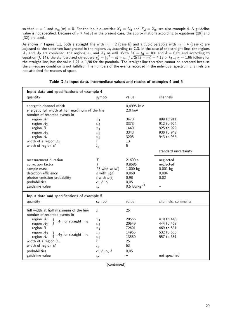
so that w = 1 and urel(w) = 0. For the input quantities X1 = Xg and X2 = Z0, see also example 4. A guidelinevalue is not specified. Because of y ≥ 4u(y) in the present case, the approximations according to equations (29) and(32) are used.

As shown in Figure C.1, both a straight line with m = 2 (case b) and a cubic parabola with m = 4 (case c) areadjusted to the spectrum background in the regions Ai according to C.3. In the case of the straight line, the regionsA1 and A2 are combined, the regions A3 and A4 as well. With M = t0 = 100 and δ = 0,05 and according toequation (C.14), the standardized chi-square χ2

s = |χ2−M + m| /√

2(M −m) = 4,18 > k1−δ/2 = 1,96 follows forthe straight line, but the value 1,21 < 1,96 for the parabola. The straight line therefore cannot be accepted becausethe chi-square condition is not fulfilled. The numbers of the events recorded in the individual spectrum channels arenot attached for reasons of space.

Table D.4: Input data, intermediate values and results of examples 4 and 5

Input data and specifications of example 4quantity symbol value channels

energetic channel widthenergetic full width at half maximum of the linenumber of recorded events in

region A1region A2region Bregion A3region A4

width of a region Aiwidth of region B

measurement durationcorrection factorsample massdetection efficiencyphoton emission probabilityprobabilitiesguideline value

n1n2ngn3n4ttg

TfM with u(M)ε with u(ε)i with u(i)α, β, γηr

0,4995 keV2,0 keV

34703373144033433208135

21600 s0,85851,000 kg0,0600,980,050,5 Bq kg−1

899 to 911912 to 924925 to 929930 to 942943 to 955

standard uncertainty

neglectedneglected0,001 kg0,0040,02––

Input data and specifications of example 5quantity symbol value channels, comments

full width at half maximum of the linenumber of recorded events in

region A1}

A1 for straight lineregion A2region Bregion A3

}

A2 for straight lineregion A4width of a region Aiwidth of region Bprobabilitiesguideline value

h

n1n2ngn3n4ttgα, β, γ, δηr

25

205562054972691149651358025630,05–

419 to 443444 to 468469 to 531532 to 556557 to 581

not specified

(continued)

29

Table D.4 (completed)

Intermediate values Example 4 Example 5quantity and calculation value value

n0 = n1 + n2 + n3 + n4n′0 = n1 − n2 − n3 + n4total width t0 = 4t of the regions Aibackground contribution z0 with standard

uncertainty u(z0) according to equation (C.12)

13394–38521293,219,7

69650–137810045766401

Results Example 4 Example 5measurand : Y AM I

quantity symbol value in Bq kg−1 unit 1

primary measurement resultstandard uncertainty associated with ydecision thresholdmeasurement effect present ?detection limitmeasurement procedure suitable ?lower confidence limitupper confidence limitbest estimate the measurandstandard uncertainty associated with zstandardized chi-squarechi-square condition fulfilled ?

yu(y)y∗

y > y∗ ?η∗

η∗ ≤ ηr ?ηlηuzu(z)χ2

sχ2

s ≤ k1−δ/2 ?

0,13460,04030,0619yes

0,1279yes

0,05580,21370,13470,0402––

26925483747yes

1497–

259782787126925483

1,21 (parabola), 4,18 (straight line)yes (parabola), no (straight line)

Annex E(informative)

Distribution function of the standardized normal distribution

The distribution function of the standardized normal distribution is defined by

Φ(t) =1√2π

∫ t

−∞exp(−v2/2) dv =

12

+1√2π

exp(−t2/2)∞∑

j=0

t2j+1

1 · 3 · · · (2j + 1)(E.1)

and its quantile kp for the probability p by Φ(kp) = p [9]. The second expression in equation (E.1) can serve forthe numerical calculation of Φ(t). The series in equation (E.1) converges for every t. Values of Φ(t) are presented inTable E.1. The relations Φ(−t) = 1− Φ(t) and k1−p = −kp apply.

The quantile kp of the standardized normal distribution can be calculated numerically as follows using the Newtoniteration procedure: With an approximation t for kp, an improved approximation t′ results from

t′ = t +√

2π exp(t2/2) (p− Φ(t)) . (E.2)

The value t = 0 can be chosen as a starting approximation.

30

Table E.1: Distribution function Φ(t) of the standardized normal distribution

t Φ(t) t Φ(t) t Φ(t) t Φ(t) t Φ(t)

0,00 0,50000,02 0,50800,04 0,51600,06 0,52390,08 0,5319

0,10 0,53980,12 0,54780,14 0,55570,16 0,56360,18 0,5714

0,20 0,57930,22 0,58710,24 0,59480,26 0,60260,28 0,6103

0,30 0,61790,32 0,62550,34 0,63310,36 0,64060,38 0,6480

0,40 0,65540,42 0,66280,44 0,67000,46 0,67720,48 0,6844

0,50 0,69150,52 0,69850,54 0,70540,56 0,71230,58 0,7190

0,60 0,72580,62 0,73240,64 0,73890,66 0,74540,68 0,7518

0,70 0,75800,72 0,76420,74 0,77040,76 0,77640,78 0,7823

0,80 0,78810,82 0,79390,84 0,79960,86 0,80510,88 0,8106

0,90 0,81590,92 0,82120,94 0,82640,96 0,83150,98 0,8365

1,00 0,84131,02 0,84611,04 0,85081,06 0,85541,08 0,8599

1,10 0,86431,12 0,86861,14 0,87291,16 0,87701,18 0,8810

1,20 0,88491,22 0,88881,24 0,89251,26 0,89611,28 0,8997

1,30 0,90321,32 0,90661,34 0,90991,36 0,91311,38 0,9162

1,40 0,91921,42 0,92221,44 0,92511,46 0,92781,48 0,9306

1,50 0,93321,52 0,93571,54 0,93821,56 0,94061,58 0,9430

1,60 0,94521,62 0,94741,64 0,94951,66 0,95151,68 0,9535

1,70 0,95541,72 0,95731,74 0,95911,76 0,96101,78 0,9625

1,80 0,96411,82 0,96561,84 0,96711,86 0,96861,88 0,9700

1,90 0,97131,92 0,97261,94 0,97381,96 0,97501,98 0,9762

2,00 0,97722,02 0,97832,04 0,97932,06 0,98032,08 0,9812

2,10 0,98212,12 0,98302,14 0,98382,16 0,98462,18 0,9854

2,20 0,98612,22 0,98682,24 0,98742,26 0,98812,28 0,9887

2,30 0,98932,32 0,98982,34 0,99042,36 0,99092,38 0,9913

2,40 0,99182,42 0,99222,44 0,99272,46 0,99302,48 0,9934

2,50 0,99382,52 0,99412,54 0,99452,56 0,99482,58 0,9951

2,60 0,99532,62 0,99562,64 0,99592,66 0,99612,68 0,9963

2,70 0,99652,72 0,99672,74 0,99692,76 0,99712,78 0,9973

2,80 0,99742,90 0,99813,00 0,99863,10 0,99903,20 0,9993

3,30 0,99953,40 0,99973,50 0,99983,60 0,99983,80 0,9999

≥4,00 1,0000

NOTE kp = t is the quantile for the probability p = Φ(t). The relations Φ(−t) = 1− Φ(t) andk1−p = −kp apply.

31

Annex F(informative)

Further terms

F.1 Background effect: measurement effect caused by the radiation background (for instance, from natural radiationsources)

F.2 Net effect: contribution of the possible radiation of a measurement object (for instance, of a radiation sourceor a radiation field) to the measurement effect

F.3 Gross effect: measurement effect caused by the background effect and the net effect

F.4 Shielding factor: factor describing the reduction of the background count rate by the shielding effect of themeasurement object

F.5 Relaxation time constant: duration in which the output signal of a linear-scale ratemeter decreases to 1/etimes the starting value after stopping the sequence of the input pulses

F.6 Background (in spectrometric measurements): number of the events of no interest in the region of a regardedline in the spectrum. The events can be due both to the background effect by the environmental radiation and alsoto the sample itself (for instance, from other lines).

Annex G(informative)

Explanatory notes

G.1 General aspects of counting measurementsA measurement of ionizing radiation consists in general at least partially in counting electronic pulses induced byionizing-radiation events. Such a measurement comprises several individual countings, but can also comprise sequencesof individual countings. Examples are the countings on samples of radioactive material or on blanks, countings forthe determination of the background effect or the countings in the individual channels of a multi-channel spectrumor in a temporal sequence in the same measurement situation. With each of the countings, either the measurementduration (time preselection) or the counting result (preselection of counts) can be fixed. On the basis of Bayesianstatistics, all countings are treated in the same way as follows (see [7]).

The pulse number N of each of the countings is taken as a separate random variable. n is the counting result and tis the counting duration (measurement duration). N has the expectation value %t, where % is the count rate or, withspectrum measurements, the spectral density. In the latter case, t is the channel width with respect to the assignedquantity, for instance, the particle energy. Either % or %t is the measurand. It is assumed that dead-time and life-timeeffects, pile-up of the pulses, and instrumental instabilities can be neglected during counting and that all the countedpulses are induced by different ionizing-radiation events which are physically independent. The pulse number N thenfollows a Poisson distribution and the pulse numbers of all the countings are independent of each another.

Irrespective of whether n pulses are recorded in a measurement of a preselected duration (or of a fixed channel width)t (time preselection) or whether the measurement duration t needed for the counting of a preselected pulse numbern is measured (preselection of counts), %t follows a gamma distribution, where % is taken as a random variable. Thenthe best estimate r of the count rate (or spectral density) % and the standard uncertainty u(r) associated with rfollow from

r = E % = n/t ; u2(r) = Var (%) = n/t2 = r/t . (G.1)

The case n = 0 results in u(r) = 0. This disappearing uncertainty of % means that % = 0 is exactly valid. But u(r) = 0is an unrealistic result because, with a finite measurement duration, one can never be sure that exactly % = 0 if nopulse happens to be recorded. This case can also lead to a zero denominator when the least-squares method accordingto DIN 1319-4 or [3] is applied and a division by u2(r) must be made. This shortcoming can be avoided by replacingall of the counting results n by n + 1 or, with a multi-channel spectrum, by a suitable combination of channels.Here, the measurement duration (or channel width) is assumed to be chosen from experience such that at least afew pulses can be expected if % > 0.

32