determination of ultimate carbonaceous bod … · determination of ultimate carbonaceous bod and...
TRANSCRIPT
DETERMINATION OF ULTIMATE CARBONACEOUS BOD
AND THE SPECIFIC RATE CONSTANT
By J. K. Stamer, J. P. Bennett, and S. W. McKenzie
U.S. GEOLOGICAL SURVEY
Open-File Report 82-645
1983
UNITED STATES DEPARTMENT OF THE INTERIOR
JAMES G. WATT, Secretary
GEOLOGICAL SURVEY
Dallas L. Peck, Director
For additional information write to:
District ChiefU.S. Geological SurveyWater Resources Division4th Floor102 East Main StreetUrbana, Illinois 61801
Copies of this report can be purchased from:
Open-File Services Section Western Distribution Branch U.S. Geological Survey Box 25425, Federal Center Denver, Colorado 80225 [Telephone: (303) 234-5888]
CONTENTS
Page
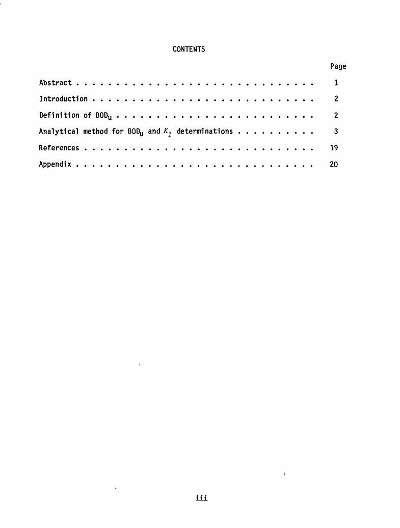
Abstract .............................. 1
Introduction ............................ 2
Definition of BODU ......................... 2
Analytical method for BODU and K^ determinations .......... 3
References ............................. 19
Appendix .............................. 20
ill
ILLUSTRATIONS
Page
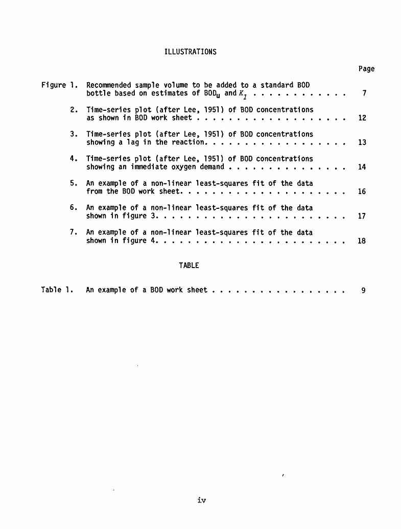
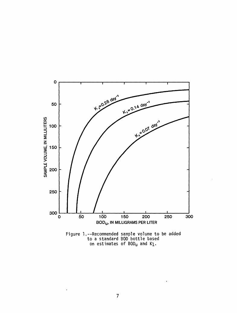
Figure 1. Recommended sample volume to be added to a standard BODbottle based on estimates of BODU and£- ............ 7
2. Time-series plot (after Lee, 1951) of BOD concentrationsas shown in BOD work sheet ................... 12
3. Time-series plot (after Lee, 1951) of BOD concentrationsshowing a lag in the reaction. ................. 13
4. Time-series plot (after Lee, 1951) of BOD concentrationsshowing an immediate oxygen demand ............... 14
5. An example of a non-linear least-squares fit of the datafrom the BOD work sheet. .................... 16
6. An example of a non-linear least-squares fit of the datashown in figure 3. ....................... 17
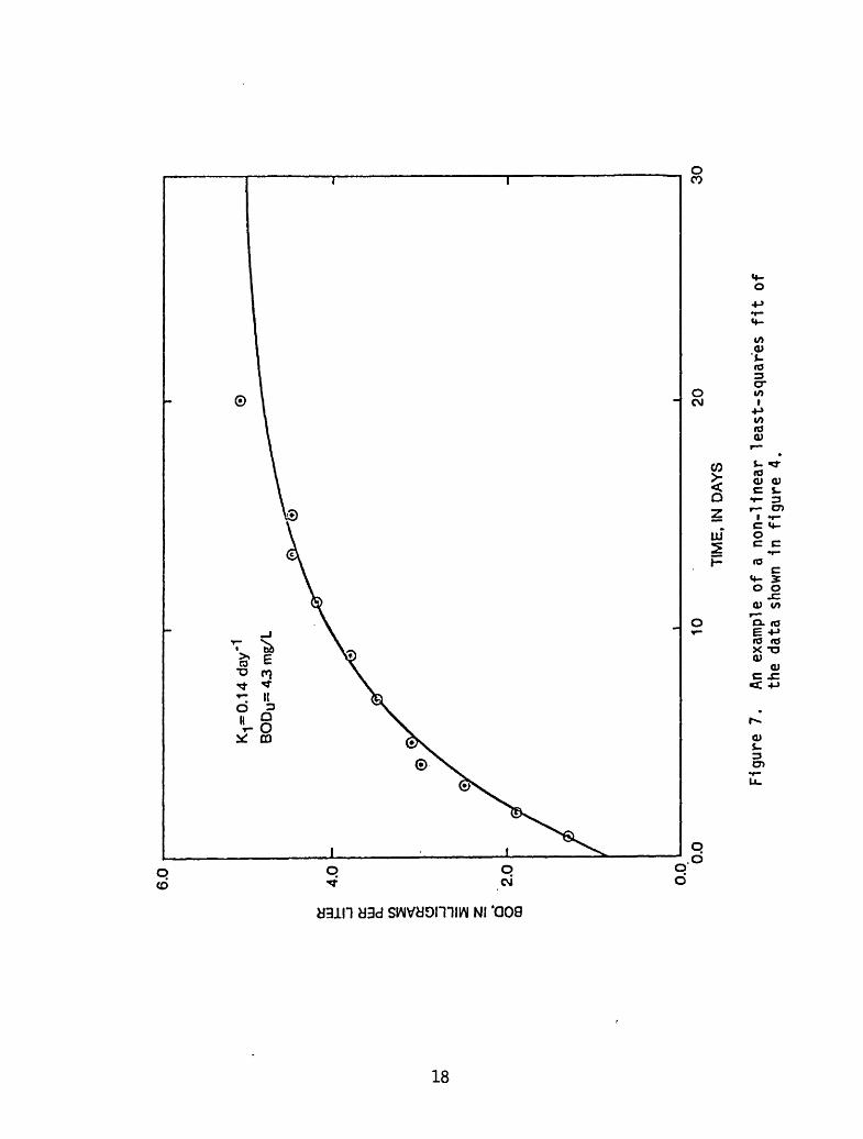
7. An example of a non-linear least-squares fit of the datashown in figure 4. ....................... 18
TABLE
Table 1. An example of a BOD work sheet ................. 9
IV
ABSTRACT
Ultimate carbonaceous biochemical oxygen demand (BODU ) and the specific rate constant (#~) at which the demand is exerted are important parameters in designing biological wastewater treatment plants and in assessing the impact of wastewater on receiving streams. An analytical method is pre sented which uses time-series concentrations of BOD, defined as the cal culated sum of dissolved oxygen (DO) losses at each time of measurement, for determining BODU and KJ. Time-series DO measurements are obtained from a water sample that is incubated in darkness at 20 degrees Celsius in the presence of nitrapyrin, a chemical nitrification inhibitor. Time-series concentrations of BOD that approximate first order kinetics can be analyzed graphically or mathematically to compute BODU and JL.

INTRODUCTION
Reliable biochemical oxygen demand (BOD) data are not only essential but the principal tool available for the rational design of biological wastewater-treatment plants and for assessing the impact of wastewater on receiving streams. However, the standard 5-day BOD, which is determined by subtracting the final concentration of dissolved oxygen (DO) from the initial concentration of DO after incubation of a sample for 5 days, does not provide the necessary information for making design decisions or for assessing the impact of wastewater on receiving streams. The cause and effect relationship cannot be defined. The needed information can be ob tained from determinations of the ultimate carbonaceous BOD (BODu )and the specific rate constant (Xj) at which it is exerted. Stamer and others (1979a) have previously evaluated several methods of BODU determination. The determination of reliable BODU and K^ values are important and indis pensable parameters in mathematical modeling of DO regimes in rivers and estuaries, an integral part of the U.S. Geological Survey's River-Quality Assessment Program (Mines and others, 1978; Bauer and others, 1978; Stamer and others, 1979b). The purpose of this paper is to present an analytical method for determining BODU and K^.
DEFINITION OF BODU
BODU is defined as the total amount of DO consumed by heterotrophic organisms to oxidize decomposable carbonaceous material (Sawyer and McCarty, 1967). Phelps (1944) theorized that the rate at which biochemical oxi dation proceeds is proportional to the remaining concentration of unoxidized carbonaceous material. In mathematical form this can be expressed as
which may be integrated between the limitsL, and L to yield£ O
L_t__
O
where, t is time, in days,
L is the concentration of remaining BODU , in milligrams per liter (mg/L) after t days,
L is the initial oxidizable concentration of BODU at t=0, and
&2 is the specific rate constant, base e, in days"1 .
Equation (2) can be rewritten to express the amount of BODU exerted, y., as-K t t
y. = L (1-e ). ' (3)
BODy and K- are determined in the laboratory usually at 20 degrees Celsius C). As with most chemical reactions, K2 is temperature dependent and
can be corrected to in-stream water temperature using the equation (Yelz,1970)
where, (K2 )T is the specific rate constant at temperature, T* in *C 9 and (K 1 } on<>n is the specific rate constant at T = 20°£.
2 <->() Cf
ANALYTICAL METHOD FOR BODy AND ^ DETERMINATIONS
1. Range of application
1.1 The method can be used to analyze natural waters, municipal waste- water, and some industrial wastewaters containing 0 to 7 mg/L BODU . Samples having a BODU ranging from about 7-40 mg/L require reaeration during the test. Samples having a BODU greater than about 40 mg/L require dilution and possible reaeration during the test.
2. Summary of method
2.1 Values of BODU and K2 are determined on the basis of time-series DO measurements of a water sample. The sample is incubated in darkness at 20°£ in the presence of nitrapyrin, a chemical nitrification inhibitor. Concen trations of DO in the BOD samples are measured using a DO meter with a self stirring BOD bottle probe. The resulting time-series concentrations of BOD, defined as the calculated sum of DO losses at each time of measurement, can be analyzed graphically or mathematically to compute BODU and ^-
In the graphical technique, described by Lee (1951) and Velz (1970), time-series concentrations of BOD (in mg/L) are plotted on a linear Y-axis, and time (£), in days, is plotted on the X-axis., usually a 25.4-cm (10-in.) scale, which is proportioned according to (l-e~ 2 ) for a specific value of Kj. Time-series concentrations of BOD that decay at that specific rate will plot as a straight line on a graph for that K2 value. Extrapolation to ultimate a of a best-fit, straight line through the time-series concentrations of BOD results directly in the BODU value.
In the mathematical technique BODU and K are computed using a non-linear least-squares method. The method uses a modified Newton iteration to mini mize the sums of the squares of the deviations of the individual time-series concentrations of BOD from equation (3). A detailed derivation of the method is given in the Appendix. The non-linear least-squares method is ideally suited to machine computation and produces directly the optimum values of BODU and K2 . Most desk-top computing systems have some means for displaying graphical results; this means should be used for comparing the observed and computed time-series concentrations of BOD.
3. Interferences
3.1 Wastewater discharges often contain residual chlorine, which can inhibit or cause a lag in the process of biochemical oxidation. Samples containing residual chlorine should be treated at the time of collection. (See step 6.1)
3.2 High concentrations of heavy metals, which include chromium, copper, lead, or mercury and other constituents such as iron, arsenic, or cyanide can inhibit the process of biochemical oxidation. Samples containing one or more of these constituents may require dilution or treatment.
3.3 Industrial wastewater discharges which are very acidic or alkaline can inhibit the process of biochemical oxidation.
4. Apparatus
4.1 Oxygen meter, (Yellow Springs Instrument Co.) a , Model No. 54 or 57, equipped with Model No. 5720 self-stirring BOD bottle probe, or equivalent.
4.2 Barometer (altimeter), capable of being read to at least the nearest 5 millimeters of mercury, (Thommen Everest), Model No. 3011, or equivalent.
4.3 BOD bottle, 300 milliliters (ml) with ground-glass stopper, (Wheaton) "800", or equivalent. Bottles should be washed thoroughly before each test in an Alconox solution or equivalent, and rinsed with distilled water.
4.4 Overcap, plastic, for BOD bottles, to prevent evaporation of water seal during incubation, (Wheaton) No. 227720, or equivalent.
4.5 BOD incubator, (Precision) Model 815, or equivalent. The BOD incubator selected should meet the following general requirements:
Maintain a uniform temperature of 20°C ± 0.5°C.Have a blower which will circulate air within the incubator.Be thermostatically controlled.
Nominal capacity should be about 0.45 cubic meter to hold 300 BOD bottles.
4.6 Aquarium pump, (Silent Giant), or equivalent; plastic air tubing, air diffusion stones, and gang valve. The aquarium pump selected should be capable of driving about 10 air diffusion stones.
4.7 Thermometer, Celsius, with a range of about 5-50°C with 0.5°C divisions, (H-B Instrument Co.) catalog No. 21223 1/2, or equivalent.
4 «8 Aeration tube, plastic, about 8 centimeters long, tapered on both ends to fit a standard 300 ml bottle. The tapered tube can be produced easily by most machine shops from 2.54-centimeter outside diameter plastic
aThe use of brand names in this report is for identification'purposes only and does not imply endorsement by the U.S. Geological Survey.

pipe. The aeration tube is convenient for reaerating BOD samples of waste- water effluent during incubation when the DO in the BOD sample is near de pletion. These samples generally foam during reaeration, and use of the aeration tube minimizes loss of sample volume as compared to reaerating with an aquarium pump equipped with air diffusion stones.
4.9 Glass beads, borosilicate, solid spherical, 5 millimeters in dia meter, (Corning) 7268 or equivalent. The glass beads should be washed thoroughly in an Alconox solution or equivalent, and rinsed with distilled water before use.
4.10 Graduated cylinder, borosilicate, 250 ml volume with 2 ml sub divisions, "~TCoTnTnin~~3oWr~o~r equivalent.
4»H Pi pets, volumetric, borosilicate, capacities of 1-50 ml (Corning) 7100, or equivalent. Grind off about 3-4 millimeters of the tip to reduce errors associated with subsampling.
4.12 Spatula, micro, stainless, Fisher catalog No. 20-401-18, or equi valent.
5. Reagents
5.1 Nitrapyrin, 2 chloro-6 (trichloromethyl) pyridine, 96-percent pure. Nitrapyrin should be kept in a tightly sealed amber bottle.
5.2 Sodium sulfite-cobalt chloride solution: Dissolve 1 g of sodium sulfite (NagSOz) and 1 small crystal (a few mg) of cobalt chloride (CoCl 9 } in 1 liter of distilled water.
5.3 Sulfuric acid (IN): Add 28 ml of concentrated sulfuric acid (H2S04 ) to about 900 ml of distilled water, mix and dilute to 1 liter.
5.4 Sodium hydroxide (IN): Add 40 g of sodium hydroxide (NaOH) to about 900 ml of distilled water, mix until dissolved, cool to about 20°C, and dilute to 1 liter.
5.5 Sodium sulfite solution (0.025N): Dissolve 1.575 g of anhydrous sodium sulfite (NajSO ) in 1,000 mL of distilled water. The solution is not stable and shoSlcrbe prepared daily or as needed.
5.6 Dilution water: Native stream water of high quality should be used as dilution water for BODU test of wastewaters and natural waters containing high concentrations of BODj. Native stream water of high quality implies that: The water has a ready-made bacterial "seed" acclimated to the types of wastewater entering the stream, lake, or estuary; the concentration of BODU is low (less than about 2-3 mg/L); and the water contains no known interferences. Dilution water should be acclimated as given in step 5.7.
5.7 Collect several liters of dilution water, aerate to saturation at 20°C, and incubate at 20°C. Measure DO concentrations daily for about 3-5 days to insure that the BODU is low. The dilution water is then ready for use. '
Procedure
6.1 If sample contains interferences, pretreat as described by the oxygen demand (biochemical) method (507) in "Standard Methods" (1975).
6.2 A decision must be made as to whether 300 ml or a lesser volume of sample is to be analyzed. The decision is based on estimates of the BODU , #2» and the desired frequency of making DO measurements on the sample. For example, no sample dilution would be required if the sample contained less than about 40 mg/L BODU ,^ was less than about 0.14 day , and DO measure ments were made when t = (r, 0.5, 1, 2, 3, 4, 5, 6, 8, 10, 12, 16, and 20 days. Figure 1 illustrates some general guidelines for sample dilutions based on a range of values of BODU and K.^ . Minimize sample dilution such that at least 4.0 mg/L of DO are depleted over the course of the test. When sample dilutions are required, make two dilutions, differing by a factor of 3 (for example, sample volumes of 50 and 150 ml).
6.3 Warm samples to 20°C ± 0.5°C. Insert air diffusion stone into the container and aerate sample, or deaerate sample if the sample is super saturated, for about 10-15 minutes. Remove air diffusion stone and allow several minutes for excess air bubbles to dissipate.
6.4 For samples that do not require dilution, proceed to step 6.8.
6.5 Measure the amount of sample to be used in the determination using a volumetric pi pet for sample volumes less than 50 ml or a graduated cylinder for sample volumes greater than 50 ml. Pour the sample from the graduated cylinder or drain the sample from the pi pet carefully down the inside of a 300 ml BOD bottle.
6.6 Fill the remainder of the BOD bottle to the neck with dilution water, carefully pouring the dilution water down the inside of the BOD bottle. Avoid entrapment of air bubbles under the neck of the BOD bottle. If air bubbles become entrapped, tap the outside of the BOD bottle.
6.7 Prepare in triplicate BOD bottles containing only dilution water. Proceed to step 6.9.
6.8 Pour the sample carefully down the inside of a BOD bottle and fill to neck of bottle. Avoid entrapment of air bubbles under neck of the BOD bottle. If air bubbles become entrapped, tap the outside of the BOD bottle.
6.9 The DO meter with probe should be turned on for at least one hour before calibration, but not the stirring motor.
6.10 Calibrate the DO meter using a wet-all method as described in the instructions manual of the Yellow Springs Instrument Co.
6.10a Insert the probe into a BOD bottle containing about 50 ml of dis tilled water. Probe, BOD bottle, and distilled water should all be at room temperature.
6.1 Ob Turn on the stirring motor.t
6.10c Switch to the temperature position and read the temperature.
50
(Ooc 01t 100
150
§LJJ
200
250
30050 100 150 200 250
BODU , IN MILLIGRAMS PER LITER
Figure 1.--Recommended sample volume to be addedto a standard BOD bottle based
on estimates of BODU and KI.
300
6.10d Determine the barometric pressure using the barometer.
6.10e Determine the solubility of oxygen, based on the temperature and barometric pressure from an oxygen-solubility table. (Manufacturer's instruction manual contains a table of oxygen solubilities at various temperatures and barometric pressures.)
6.1 Of Switch to calibration and position the needle to the correct DO reading using the calibration knob.
6.10g Turn off the stirring motor before removing the probe from the BOD bottle.
6.11 To measure concentration of DO of a sample, carefully insert the self-stirring probe into a BOD bottle to avoid entrapment of air.
6.12 Turn on the stirring mechanism.
6.13 Allow about 1-2 minutes for DO reading to stabilize.
6.14 Record the date, time, and DO concentration (in column titled "DISS 02") on a form similar to that shown in table 1.
6.15 Turn off the stirring mechanism, remove the probe and rinse with distilled water.
6.16 Add about 3-5 small crystals of nitrapyrin to the BOD sample. Do not add further nitraphyrin during the incubation period.
6.17 Carefully insert the glass stopper and tip the BOD bottle to one side to check for trapped air. If an air bubble exists, remove the glass stopper and add just enough glass beads to displace it. Replace the glass stopper and check again for trapped air. If the bubble remains, add additional glass beads. If no bubble exists, create a water seal using distilled water and place overcap on the BOD bottle. Incubate the sample (in darkness) at 20°C +_ 0.5°C.
6.18 After the initial DO reading, measure the DO concentration 10-12 times during the incubation period. Suggested incubation periods and measurements are: (1) 20-day incubation period with DO measurements made at t = 0, 0.5, 1, 2, 3, 4, 5, 6, 8, 10, 12, 16, and 20 days and (2) 5-7 day incubation period with DO measurements at 12-15 hour intervals provided that the BOD reaction is proceeding normally (that is, no initial lag because of the presence of a substance toxic to the bacteria).
6.19 After each incubation period, remove the BOD bottle from the incubator, remove the plastic overcap, pour off the water seal, remove the ground-glass stopper and measure the DO concentration following steps 6.9 through 6.17.
Note - Carefully insert the calibrated DO probe (step 6.10a) into a BOD bottle during sequential measurements of DO concentrations to minimize loss of sample volume. *
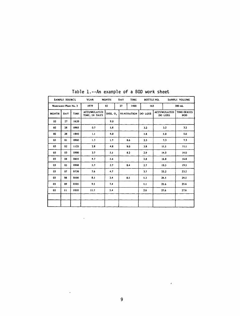
Table l.--An example of a BOD work sheetSAMPLI: SOURCE YEAR MONTH DAY TIME BOTTLE NO. SAMPLI: VOLUME
Waslcwalcr Plant No. 3
MONTH
02
02
02
03
03
03
03
03
03
03
03
03
DAY
27
28
28
01
02
03
04
05
07
08
09
II
TIMi:
1620
0905
1840
0900
1125
0900
0855
0900
0730
0500
0505
1010
1979 02 27 1400 163 300 mL
ACCUMULATED TIME, IN DAYS
0.7
I.I
1.7
2.8
3.7
4.7
5.7
7.6
8.5
9.5
11.7
DISS. 0 2
9.0
5.8
4.0
1.7
4.8
5.1
5.4
2.7
4.7
3.4
7.4
5.4
RKAF.RATION
8.6
8.0
8.2
8.4
8.5
DO LOSS
3.2
1.8
2.3
3.8
2.9
2.8
2.7
3.7
1.3
I.I
2.0
ACCUMULATED DO LOSS
3.2
5.0
7.3
II. 1
14.0
16.8
19.5
23.2
24.5
25.6
27.6
TIME-SERIES BOD
3.2
5.0
7.3
ll.l
14.0
16.8
19.5
23.2
24.5
25.6
27.6
6.20 If the BOD sample does not require reaeration, (DO concentration will not fall below 2 mg/L by the next reading), then replace it 1n the incubator (as in step 6.17).
6.21 If the BOD sample requires reaeration (DO concentration may fall below 2 mg/L by next reading), use a reaeration tube as indicated in steps 6.22 to 6.24.
6.22 Place one end of the reaeration tube into the top of a clean empty BOD bottle, and place the other end into the top of the BOD sample bottle to be reaerated.
6.23 Hold the bottles, one in each hand, and vigorously shake the bottles back and forth for about 30 seconds.
6.24 Set the two bottles down, with the BOD sample bottle upright and allow time for the sample to drain back into original BOD sample bottle,
6.25 Allow time for the air bubbles in the sample to dissipate.
6.26 Measure the DO concentration (reaeration) and record results ac cording to steps 6.9 through 6.17.
7. Calculations
7.1 Determine carbonaceous BODU and ^ using either the graphical or mathematical techniques. Either technique provides concentrations of 5- and 20-day BODs.
7.2 To use the mathematical technique, proceed to step 7.12.
7.3 Calculate the accumulated time of incubation for each DO reading to the nearest 0.1 day in column titled "ACCUMULATED TIME, IN DAYS" (table 1) with accuracy to the nearest tenth of a day.
7.4 Calculate the "ACCUMULATED DO LOSS" equal to the oxygen demand exerted in the BOD bottle. See example in table 1. If dilution water was not used, these are the BOD values used to determine the specific rate constant, K^*
7.5 Calculate the "BOD of dilution water". If dilution water was used, these are the average values taken from the three BOD tests on dilu tion water only (see step 6.7).
7.6 Calculate the time-series concentrations of BOD of the sample when dilution water has been used from
300 BODR - (300-VJ BODn BODS = ?_ § D
10
where,BODS = BOD of sample, in mg/L,
BODg - BOD of bottle, in mg/L,
V s = Volume of sample used in bottle, in ml,
and, BOD0 = BOD of dilution water in mg/L.
Record the value in column "TIME-SERIES BOD" in table 1 and use these to determine the values of BODU and
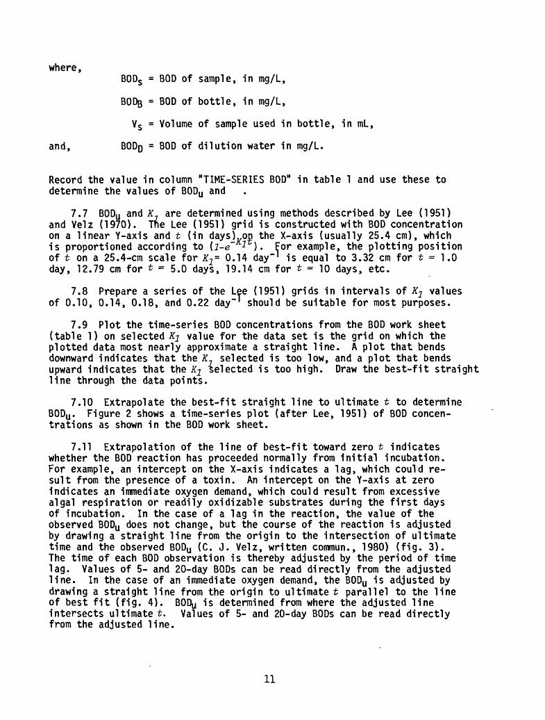
7.7 BODU and K are determined using methods described by Lee (1951) and Velz (1970). The Lee (1951) grid is constructed with BOD concentration on a linear Y-axis and t (in days) on the X-axis (usually 25.4 cm), which is proportioned according to (i-e * ) For example, the plotting position of t on a 25.4-cm scale for K2 = 0.14 day"' is equal to 3.32 cm for t = 1.0 day, 12.79 cm for £ = 5.0 days, 19.14 cm for t = 10 days, etc.
7.8 Prepare a series of the Lee (1951) grids in intervals of K2 values of 0.10, 0.14, 0.18, and 0.22 day"' should be suitable for most purposes.
7.9 Plot the time-series BOD concentrations from the BOD work sheet (table 1) on selected K2 value for the data set is the grid on which the plotted data most nearly approximate a straight line. A plot that bends downward indicates that the K selected is too low, and a plot that bends upward indicates that the K2 ielected is too high. Draw the best-fit straight line through the data points.
7.10 Extrapolate the best-fit straight line to ultimate t to determine BODU . Figure 2 shows a time-series plot (after Lee, 1951) of BOD concen trations as shown in the BOD work sheet.
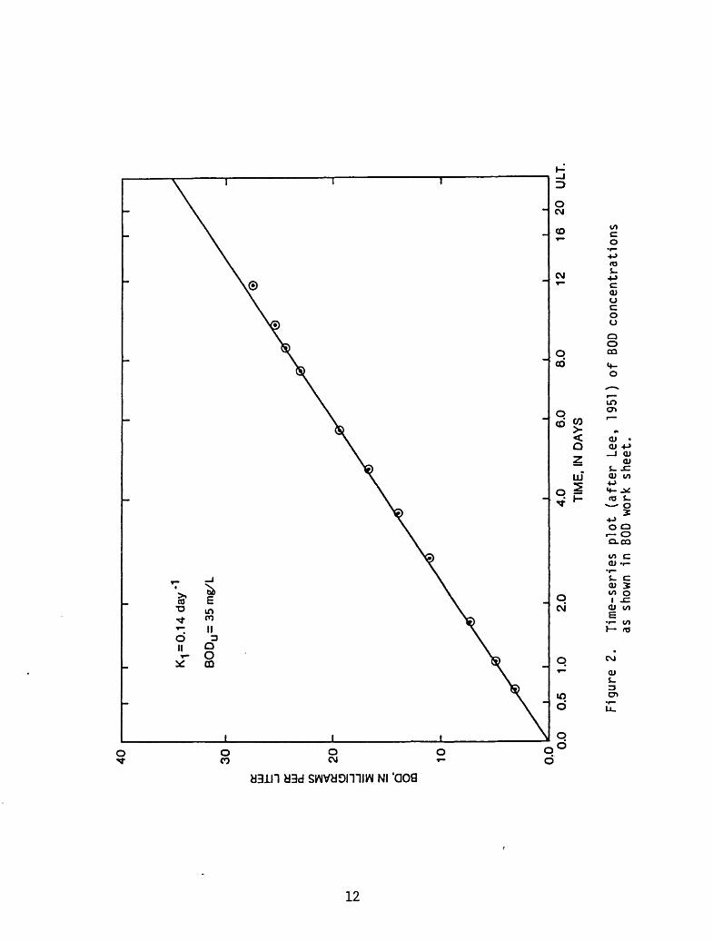
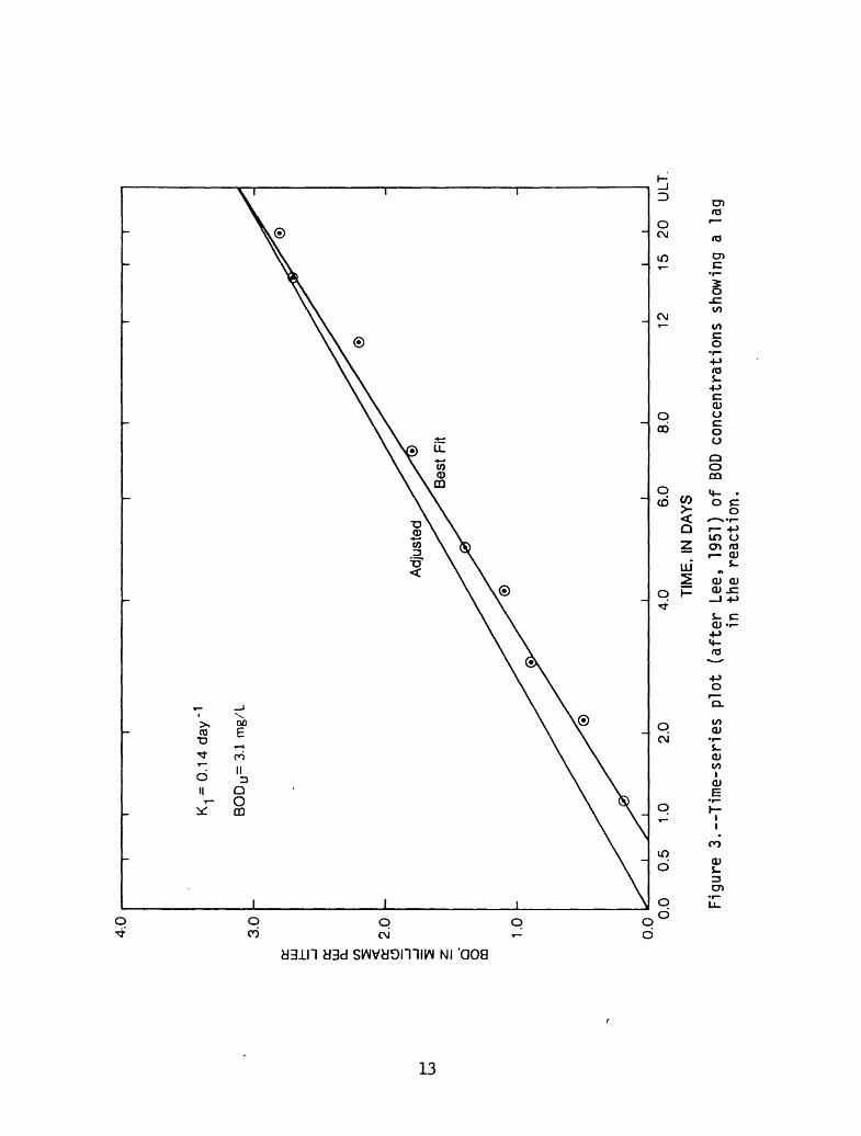
7.11 Extrapolation of the line of best-fit toward zero t indicates whether the BOD reaction has proceeded normally from initial incubation. For example, an intercept on the X-axis indicates a lag, which could re sult from the presence of a toxin. An intercept on the Y-axis at zero indicates an immediate oxygen demand, which could result from excessive algal respiration or readily oxidizable substrates during the first days of incubation. In the case of a lag in the reaction, the value of the observed BODU does not change, but the course of the reaction is adjusted by drawing a straight line from the origin to the intersection of ultimate time and the observed BODU (C. J. Velz, written commun., 1980) (fig. 3). The time of each BOD observation is thereby adjusted by the period of time lag. Values of 5- and 20-day BODs can be read directly from the adjusted line. In the case of an immediate oxygen demand, the BODU is adjusted by drawing a straight line from the origin to ultimate t parallel to the line of best fit (fig. 4). BODU is determined from where the adjusted line intersects ultimate t. Values of 5- and 20-day BODs can be read directly from the adjusted line.
11
40
UJ cc LU a. cc
20
o O
O
CO
10 0.0
i r
K-i =
0.1
4 d
ay*
BO
DU
= 3
5 m
g/L
0.0
0.5
1.0
2.0
4.0
6.0
TIM
E,
IN D
AY
S8.
012
16
20
ULT
.
Fig
ure
2.
T
ime-s
eries
plo
t (a
fter
Lee,
19
51)
of
BOD
conce
ntr
atio
ns
as
show
n in
BO
D w
ork
sheet.
ei
BOD, IN MILLIGRAMS PER LITER
CO
CD
CO
CD I
CO CD
CD CO
oc-h
-hrt
- CD
rt- r 3" CD CD CD
w-sCD « Ol VOo cn rt-
o -h
COooo o3 oCD
-S Ol
O=3 CO
3 (Q
p b
COb
p cn
H O
2m
zoI o
o
00b
cn
N)o
CDO Oc
IIU)
3 oa
II O
a0)
-p
K^
0.1
4 da
y'1
BO
DU
= 4
3 m
g/L
0.0
0.5
1.0
4.0
6.0
TIM
E.
IN D
AY
S8.
012
16
20
ULT
.
Fig
ure
4.
T
ime
-se
rie
s plo
t (a
fte
r Le
e,
1951
) o
f BO
D co
nce
ntr
atio
ns
show
ing
an
Imm
edia
te
oxyg
en
dem
and.
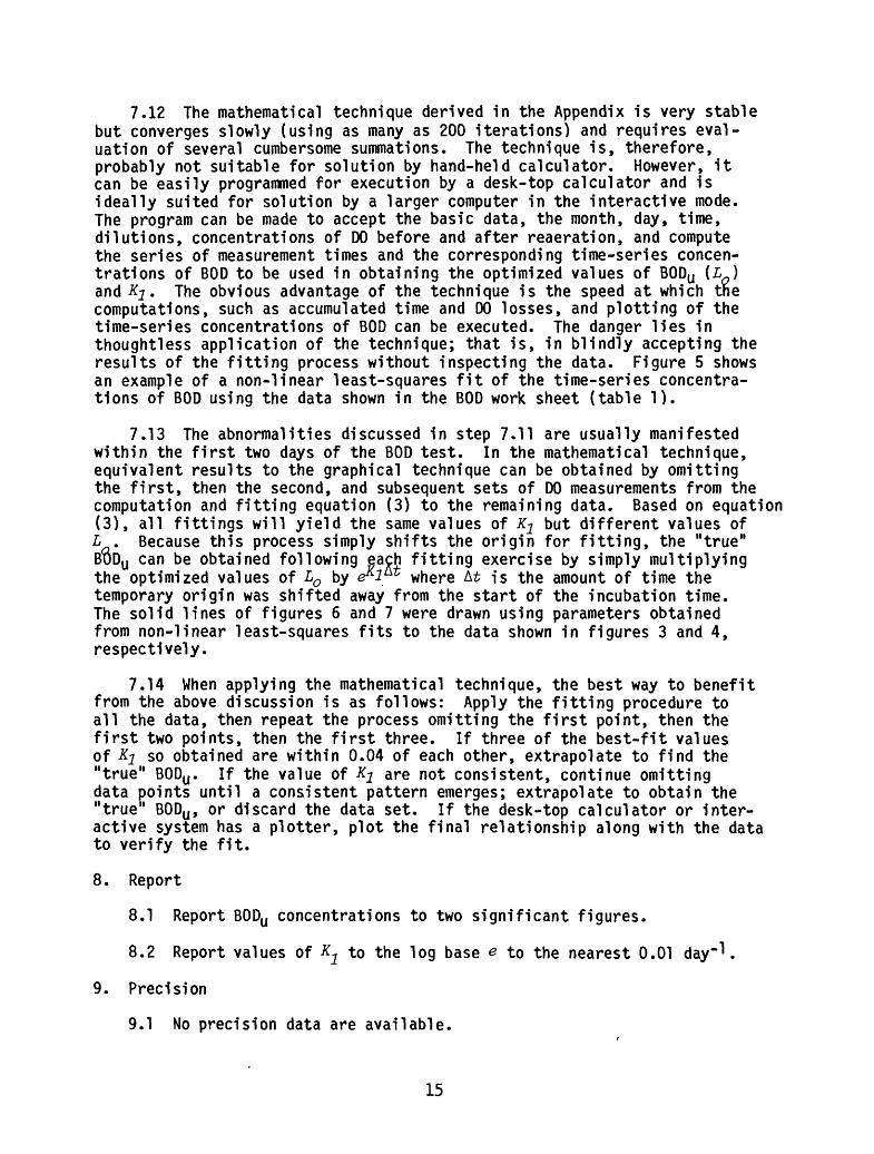
7.12 The mathematical technique derived in the Appendix is very stable but converges slowly (using as many as 200 iterations) and requires eval uation of several cumbersome summations. The technique is, therefore, probably not suitable for solution by hand-held calculator. However, it can be easily programmed for execution by a desk-top calculator and is ideally suited for solution by a larger computer in the interactive mode. The program can be made to accept the basic data, the month, day, time, dilutions, concentrations of DO before and after reaeration, and compute the series of measurement times and the corresponding time-series concen trations of BOD to be used in obtaining the optimized values of BODU (L ) and KI. The obvious advantage of the technique is the speed at which tne computations, such as accumulated time and DO losses, and plotting of the time-series concentrations of BOD can be executed. The danger lies in thoughtless application of the technique; that is, in blindly accepting the results of the fitting process without inspecting the data. Figure 5 shows an example of a non-linear least-squares fit of the time-series concentra tions of BOD using the data shown in the BOD work sheet (table 1).
7.13 The abnormalities discussed in step 7.11 are usually manifested within the first two days of the BOD test. In the mathematical technique, equivalent results to the graphical technique can be obtained by omitting the first, then the second, and subsequent sets of DO measurements from the computation and fitting equation (3) to the remaining data. Based on equation (3), all fittings will yield the same values of K^ but different values of L . Because this process simply shifts the origin for fitting, the "true" BuDu can be obtained following each fitting exercise by simply multiplying the optimized values of L0 by AAt where At is the amount of time the temporary origin was shifted away from the start of the incubation time. The solid lines of figures 6 and 7 were drawn using parameters obtained from non-linear least-squares fits to the data shown in figures 3 and 4, respectively.
7.14 When applying the mathematical technique, the best way to benefit from the above discussion is as follows: Apply the fitting procedure to all the data, then repeat the process omitting the first point, then the first two points, then the first three. If three of the best-fit values of KI so obtained are within 0.04 of each other, extrapolate to find the "true" BODU . If the value of KI are not consistent, continue omitting data points until a consistent pattern emerges; extrapolate to obtain the "true" BODU , or discard the data set. If the desk-top calculator or inter active system has a plotter, plot the final relationship along with the data to verify the fit.
8. Report
8.1 Report BODU concentrations to two significant figures.
8.2 Report values of ^ to the log base & to the nearest 0.01 day1 .
9. Precision
9.1 No precision data are available.
15

40
30
a: cc Ul
Q.
20
O
O
OQ
10 0.0
1^
=0
.14
dayl
BO
Du
= 3
4mg
/L
0.0
1020
30
TIM
E,
IN D
AY
S
Fig
ure
5.
An
exam
ple
of
a non-lin
ear
lea
st-s
qu
are
s fit
of
the
data
fr
om t
he
BOD
wor
k sh
eet.

cc Hi o:
ffi o Cf
O
TIM
E,
IN D
AY
S
Figu
re 6
. An
ex
ampl
e of
a
non-
line
ar
leas
t-sq
uare
s fi
t of
the
da
ta
show
n in
fi
gure
3.
6.0
4.0
oo
o:
LU Q.
CO <
o: o
o CD
K-j-O
/Ud
ay'1
BO
DU=
43
mg/
L
2.0
0.0
0.0
1020
30
TIM
E,
IN D
AY
S
Fig
ure
7.
An
ex
ampl
e o
f a
no
n-lin
ea
r le
ast
-square
s fit
of
the
data
sh
own
1n figure
4.
REFERENCES
American Public Health Association, American Water Works Association and Water Pollution Control Federation, 1975, Standard methods for the exam ination of water and wastewater, 14th ed. American Public Health Associ ation, Washington, D. C., 1193 p.
Bauer, D. P., Steele, T. D., Anderson, R. D., 1978, Analysis of waste-load assimilative capacity of the Yampa River, Steamboat Springs to Hayden, Routt County, Colorado: U.S. Geological Survey Water-Resources Investi gation 77-119, 69 p.
Hines, W. G., McKenzie, S. W., Rickert, D. A., and Rinella, F. A., 1978, Dissolved-oxygen regimen of the Willamette River, Oregon, under conditions of basinwide secondary treatment: U.S. Geological Survey Circular 715-1, 52 p.
Lee, J. D., 1951, Simplified method for analysis of B.O.D. data - a dis cussion: Sewage and Industrial Wastes, no. 23, p. 164-166.
Phelps, E. G., 1944, Stream sanitation: New York, John Wiley, 209 p.
Sawyer, C. N. and McCarty, P. L., 1967, Chemistry for sanitary engineers: New York, McGraw-Hill, 518 p.
Stamer, J. K., McKenzie, S. W., Cherry, R. N., Scott, C. T., and Stamer, S. L., 1979a, Methods of ultimate carbonaceous BOD determination: Journal Water Pollution Control Federation, v. 51, no. 5, p. 918-925.
Stamer, J. K., Cherry, R. N., Faye, R. E., and Kleckner, R. L., 1979b, Magnitudes, nature, and effects of point and nonpoint discharges in the Chattahoochee River basin, Atlanta to West Point Dam, Georgia: U.S. Geological Survey Water-Supply Paper 2059, 65 p.
19
APPENDIX
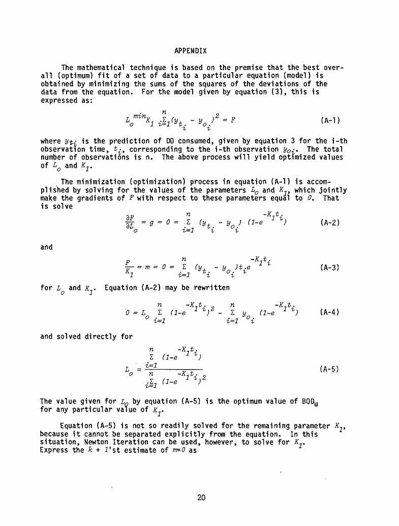
The mathematical technique is based on the premise that the best over all (optimum) fit of a set of data to a particular equation (model) is obtained by minimizing the sums of the squares of the deviations of the data from the equation. For the model given by equation (3), this is expressed as:
where y-tj is the prediction of DO consumed, given by equation 3 for the i-th observation time, t^, corresponding to the i-th observation y0^. The total number of observations is n. The above process will yield optimized values of LO and K^.
The minimization (optimization) process in equation (A-l) is accom plished by solving for the values of the parameters L0 and ^, which jointly make the gradients of F with respect to these parameters equal to 0. That is solve
|| = g = o = -Z (y - y ) (1-e 2 ^ ) (A-2) o i=l i i
andYL J{'f~
L- = m = 0 = Z (y - y )t.e l * (A-3) A i j-i I*. o. ^
for L and x . Equation (A-2) may be rewritten
n -K t. n -K t.0 = L Z (1-e 1 ^ )^ - Z y (1-e 1 *) (A-4)o . . ^ s o .
and solved directly forn ~K2 ti
i=l________ YI K "t T~> / ** ^. IS \ £j
(A-5!
The value given for LQ by equation (A-5) is the optimum value of BODU for any particular value of x? .
Equation (A-5) is not so readily solved for the remaining parameter K because it cannot be separated explicitly from the equation. In this situation, Newton Iteration can be used, however, to solve for K Express the k + 1'st estimate of rn=o as
20
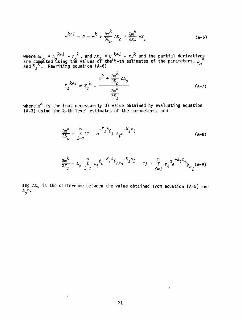
. , , r . m = 0 = m +U, + -AK (A-6)
where A£ = L - L , and Atf? = £ - tf and the partial derivatives are competed Rising th% values or the^-th estimates of the parameters, L and &2 Rewriting equation (A-6)
k 3m Ar m -/ - kL
where m is the (not necessarily 0) value obtained by evaluating equation (A-3) using the fc-th level estimates of the parameters, and
n
ot.e (A-8)^
-£-t. n 1 ^ -, , v , 2 - 2) + L t. e
^
and &L0 is the difference between the value obtained from equation (A-5) and
21