determining ability to pay in virginia’s public schools analyzing the lci · fall 08 katie baugh...

08Fall

Katie Baugh Carrie Hartgrove Erya Yang December 13th, 2015

Determining Ability to Pay in Virginia’s Public Schools Analyzing the LCI

2

Table of Contents Executive Summary ...................................................................................................................... 1 Current Local Composite Index .................................................................................................. 2 Criticisms ....................................................................................................................................... 2 Potential Solutions ........................................................................................................................ 3 How to Measure Success .............................................................................................................. 3 Fairness versus Stability ................................................................................................................. 3 Data ................................................................................................................................................ 4 Modeling a New LCI ..................................................................................................................... 4 Component Adjusted Models ......................................................................................................... 5

Comparison of Variation Across Models Within Time Periods .................................................. 5 Comparison of Variation Across Models Across Time Periods ................................................. 7 Fairness Analysis of the Models ................................................................................................. 7

Population Adjusted Models ........................................................................................................... 9 Comparison of Variation Across Models Within Time Periods .................................................. 9 Comparison of Variation Across Models Across Time Periods ............................................... 11 Fairness Analysis of the Models ............................................................................................... 11

Conclusion .................................................................................................................................... 13 Additional Variables ................................................................................................................... 13 Regression Analysis .................................................................................................................... 13 Data and Methodology .................................................................................................................. 13 Results and Conclusions of Model 1 ............................................................................................ 14 An Alternate Measure of Ability to Pay ....................................................................................... 15 Ranking Analysis ........................................................................................................................ 17 Ranking disparity between LCI and Fiscal Measures ................................................................... 17 Ranking stability between 2008-2010 Indices and 2010-2012 Indices for LCI and Fiscal Measures ....................................................................................................................................... 19 Case Analysis for Extreme LCI and Fiscal Ranking Disparities ........................................... 20 Bristol City .................................................................................................................................... 20 Harrisonburg City ......................................................................................................................... 21 Richmond City .............................................................................................................................. 21 King William County .................................................................................................................... 21 Poquoson City ............................................................................................................................... 22 Examples from Other States ...................................................................................................... 22 Bibliography ................................................................................................................................ 25 Appendix 1: Maps ....................................................................................................................... 27 Appendix 2: Ranking Measures ................................................................................................ 47 Appendix 3: Regression Analysis .............................................................................................. 50

1

Executive Summary

Accomplished: Ø Analyzed LCI and criticisms of disparity Ø Created new weighting schemes for the LCI Ø Analyzed variation between new LCI models and original model Ø Determined the most stable models and discussed fairness issues Ø Determined which data might affect the composite index Ø Created regression models to analyze significance of additional variables Ø Analyzed distribution of rankings of fiscal measures and LCI Ø Examined extreme cases of disconnected ranking structures and identified potential

causes for the disparities Ø Explored other state’s methods for determining education funding

Recommendations and Conclusions: Ø The original LCI does a good job at reflecting the ability to pay of localities Ø Fiscal ranking measures may do a better job of measuring ability to pay, however we

recommend that the fiscal rankings are simply taken into consideration and analyzed further before any renegotiation of the current LCI

Ø Consider the stability issue; balance the reflectiveness of LCI to its component variables and the desirable stability level for budgeting purpose

2

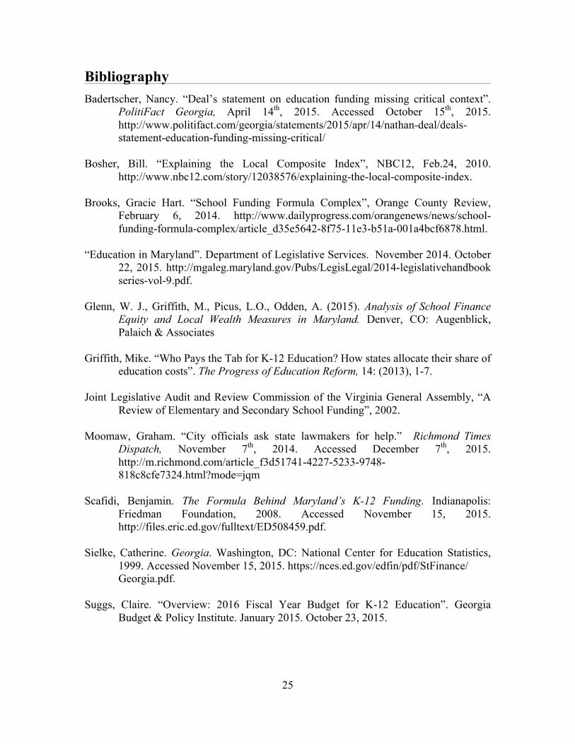
Current Local Composite Index The state government and the local governments jointly share the burden of funding

Virginia’s K-12 public education system.1 To distribute state funding for education fairly among localities, each locality’s ability to pay must be measured and funding must be disbursed accordingly. The State of Virginia determines each locality’s capacity to fund their school system with the Local Composite Index (LCI) in a manner unlike any other states.2 The LCI measures ability to pay for education, through three sources of local revenue: True Property Value, Adjusted Gross Income (AGI), and Local Sales Tax. The three components are assigned weights of 50%, 40%, and 10%, respectively. 3 A locality’s average daily student membership (ADM) and total population are used to standardize these components to create population specific indices. Each of these indices carries a weight of 2/3 and 1/3, respectively, and is added and multiplied by a weight of 45% to determine the total state funding provided per locality.4

In theory, the calculated LCI ranges from 0 to above 1.0 and reflects the amount of money a locality must contribute to education funding per dollar spent. A lower LCI indicates that a locality is less able to pay for education whereas a high LCI indicates that a locality has a high ability to pay for education. For the sake of fairness, the LCI is artificially capped at 0.8 to ensure that all localities receive at least 20% of its education funding from the state.5

Criticisms A common complaint of the LCI is the large disparity between localities in terms of

actual education expenditures and ability to pay.6 In other words, some counties might have a high fiscal capacity, but that capacity may not be adequately reflected in the calculation of their LCI. For example, after the financial crisis of 2008, property values in northern Virginia fell at a faster rate than property values in Richmond. This effect was captured by the LCI, since property value is weighted at 50% and the LCI of northern Virginia counties fell more than LCI’s of Richmond area counties in 2008. The problem remains that northern Virginia is still wealthier than Richmond but the relative wealth and ability to pay of northern Virginia to Richmond is not reflected by the LCI. 7 Another relatively common complaint is that cities are not accurately funded by the current LCI. This may be due to a number of things including high amounts of

1 Joint Legislative Audit and Review Commission of the Virginia General Assembly, “A Review of Elementary and Secondary School Funding”, 2002, 1. 2 Ibid, 125. 3 Ibid, 154. 4 Ibid. 5 Ibid. 6 Virginia Education Association, Inc., “Virginia’s Education Disparities FY 2008-09”. http://www.veanea.org/assets/document/disparity-2010-07b.pdf. For data , we used the Virginia Department of Education, http://www.doe.virginia.gov/school_finance/budget/ 7Gracie Hart Brooks, “School Funding Formula Complex”, Orange County Review, February 6,2014. http://www.dailyprogress.com/orangenews/news/school-funding-formula-complex/article_d35e5642-8f75-11e3-b51a-001a4bcf6878.html. Bill Bosher, “Explaining the Local Composite Index”, NBC12, Feb.24, 2010. http://www.nbc12.com/story/12038576/explaining-the-local-composite-index.

3

fiscal stress due to high poverty density8, or it may be due to differences between average daily membership and total population.

Potential Solutions In an effort to change how the current index reflects the reality of ability to pay in

localities, we have generated new LCI models with varying component weights and varying population weights. We believe that these different weighting schemes reflect on the accuracy of the current LCI to measure ability-to-pay by singling out the effects of its components. We have also run regression models on different variables to determine whether changes in demographic and other variables are associated with changes in LCI. Our last analytical step has been to compare the ranking of the LCI with the ranking of certain fiscal measures to determine whether LCI reflects fiscal measures of ability to pay, and what causes the disparity, if any.

How to Measure Success Fairness

One major question we have run into is how a successful index will be judged. In our eyes, success can take on different shapes. Either it can be the most “fair” or it can be the most stable. However fairness in and of itself is an ambiguous term. For smaller rural counties, fair may mean receiving additional aid to account for a shrinking tax base or a growing free and reduced lunch student population. For larger urban areas, fair may mean stability in funding to better plan for district growth or growing funding to keep pace with a growing population. There also is an issue of what fair means across districts. In an urban district looking to attract more students, fairness may be perceived as the ability to keep expected quality of education high to attract new students, whereas in rural counties, fairness may be shouldering less of the education funding in order to focus on small business development.

To better see the distribution of funds and how different indices change the LCI distribution, we have analyzed maps of the variation between our modeled LCI and the original LCI. Any patterns we may see here will show whether the model we are observing is in fact beneficial to the right kind of locality. We have measured variation of our test indices compared to the original LCI. It would be a poor policy decision to select a model that would cause significant initial variation. It would be nearly impossible to pass these changes through the legislature. Our ideal model would have to have small amounts of variation compared to the original index, as well as a beneficial pattern of change across localities.

Stability We modeled the original LCI and our test indices across time. We have looked for the relative consistency in LCI across years and wish to see stability of the index across time. It would be a poor policy decision to change the current model to one that is volatile across years, which would cause budgeting issues. On the other hand, we want the model to be sensitive to

8 Graham Moomaw, “City officials ask state lawmakers for help,” Richmond Times Dispatch, November 7th, 2014. Accessed December 7th, 2015. http://m.richmond.com/article_f3d51741-4227-5233-9748-818c8cfe7324.html?mode=jqm

4

changes of actual ability to pay. For instance, 2008 financial crisis and the following recovery greatly affected property value. We want the LCI to reflect the effect of financial crisis on ability to pay, but we do not want disproportionately capture the financial crisis’ effects impact on property value.

Data The base for all of our analysis comes from VDOE’s calculations of the LCI. The fiscal

data we have gathered comes from the Virginia Department of Housing and Community Development’s Commission on Local Government (CLG). This group “promotes and preserves the viability of Virginia’s local governments by fostering positive intergovernmental relations.”9 The CLG develops and distributes the measure of revenue capacity per capita, revenue effort, and median household income.10

In addition to these fiscal variables, we will add variables such as median house price, population density, number of students eligible for free and reduced lunch, and number of limited English proficiency (LEP) students to a regression model. We have found these datasets through the U.S. Census and through the Virginia Department of Education.

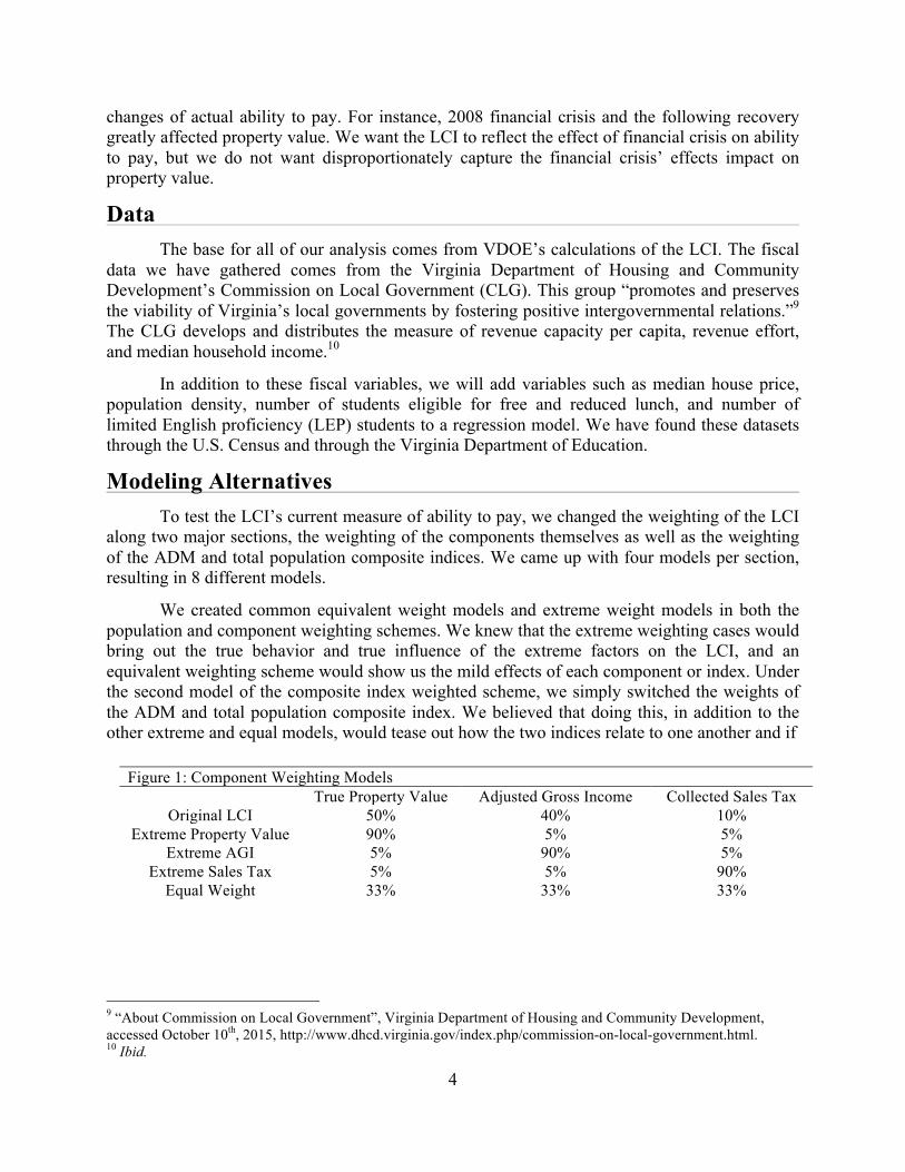
Modeling Alternatives To test the LCI’s current measure of ability to pay, we changed the weighting of the LCI

along two major sections, the weighting of the components themselves as well as the weighting of the ADM and total population composite indices. We came up with four models per section, resulting in 8 different models.

We created common equivalent weight models and extreme weight models in both the population and component weighting schemes. We knew that the extreme weighting cases would bring out the true behavior and true influence of the extreme factors on the LCI, and an equivalent weighting scheme would show us the mild effects of each component or index. Under the second model of the composite index weighted scheme, we simply switched the weights of the ADM and total population composite index. We believed that doing this, in addition to the other extreme and equal models, would tease out how the two indices relate to one another and if

9 “About Commission on Local Government”, Virginia Department of Housing and Community Development, accessed October 10th, 2015, http://www.dhcd.virginia.gov/index.php/commission-on-local-government.html. 10 Ibid.

Figure 1: Component Weighting Models True Property Value Adjusted Gross Income Collected Sales Tax

Original LCI 50% 40% 10% Extreme Property Value 90% 5% 5%

Extreme AGI 5% 90% 5% Extreme Sales Tax 5% 5% 90%

Equal Weight 33% 33% 33%

5

Figure 2: ADM and Per Capita Composite Index Weighting Models ADM Composite Index Total Per Capita Composite Index

Original LCI 67% 33% Equal Weights 50% 50%

Reversed Weights 33% 67% Extreme Per Capita 0% 100%

Extreme ADM 100% 0%

To conduct our analysis, we mapped out the sign change in LCI between the original LCI and our modeled LCI during the 2008-2010 index and the 2010-2012 index. We chose to focus our main analysis on the 2008-2010 index as well as the 2010-2012 index. These indices represent the beginning of the recession and the subsequent recovery. We believe that these two indices would show the largest variation in LCI due the effects of the recession. We also mapped out the LCI change itself in a heat map to demonstrate where the largest gains and losses were. In addition to visually mapping the variation, we modeled the variation between the original LCI and our model in a bar chart by adding the absolute value of the difference between the original model and our model. Again this was conducted within the 2008-2010 index as well as the 2010-2012 index. Initially, we used the capped LCI data, however we quickly realized that this would exclude areas such as northern Virginia from our map analysis. We then decided to use the capped LCI data for variation analysis and the uncapped LCI data as the base for mapping. We decided that looking at the mapped uncapped LCI would demonstrate the pattern behind how certain components or population indices behave. The capped variation between indices would be the best representation of the actual variation of the model; it would be over-counting to include variation in LCI for localities that have already exceeded the cap.

The final piece of our analysis of the different models is the variation across years of the different models we created. If there were larger variations across years in our new model versus the original model, we would note that for our final policy analysis. We used only capped data for this variation because, in reality, the LCI would only vary significantly for those localities that had not hit the cap. If there were wild fluctuations for areas above the cap, that variation would not matter and could potentially bias our results.

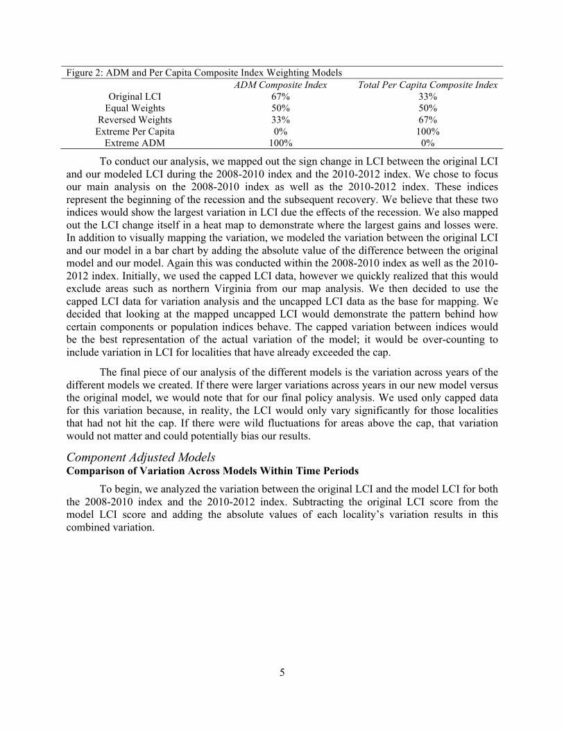
Component Adjusted Models Comparison of Variation Across Models Within Time Periods To begin, we analyzed the variation between the original LCI and the model LCI for both the 2008-2010 index and the 2010-2012 index. Subtracting the original LCI score from the model LCI score and adding the absolute values of each locality’s variation results in this combined variation.

6

Figure 3: Sum of absolute value of locality LCI 2008-2010 variance, varying component weights

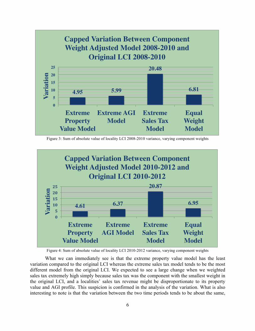
Figure 4: Sum of absolute value of locality LCI 2010-2012 variance, varying component weights

What we can immediately see is that the extreme property value model has the least variation compared to the original LCI whereas the extreme sales tax model tends to be the most different model from the original LCI. We expected to see a large change when we weighted sales tax extremely high simply because sales tax was the component with the smallest weight in the original LCI, and a localities’ sales tax revenue might be disproportionate to its property value and AGI profile. This suspicion is confirmed in the analysis of the variation. What is also interesting to note is that the variation between the two time periods tends to be about the same,

4.95 5.99

20.48

6.81

0

5

10

15

20

25

Extreme Property

Value Model

Extreme AGI Model

Extreme Sales Tax

Model

Equal Weight Model

Vari

atio

nCapped Variation Between Component Weight Adjusted Model 2008-2010 and

Original LCI 2008-2010

4.61 6.37

20.87

6.95

0510152025

Extreme Property

Value Model

Extreme AGI Model

Extreme Sales Tax

Model

Equal Weight Model

Vari

atio

n

Capped Variation Between Component Weight Adjusted Model 2010-2012 and


7

with only property value and AGI models changing significantly. This was somewhat expected because these two years represented the economic recession and the subsequent recovery, so we expect both property value and AGI to increase between these two years.

Fairness Analysis of the Models

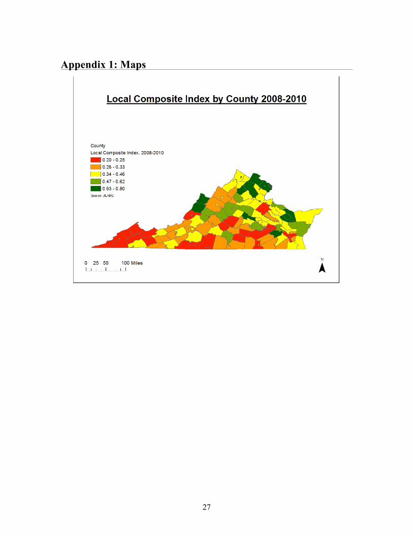
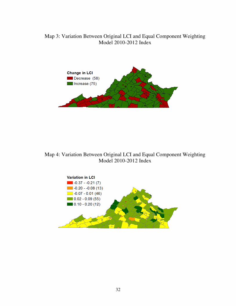
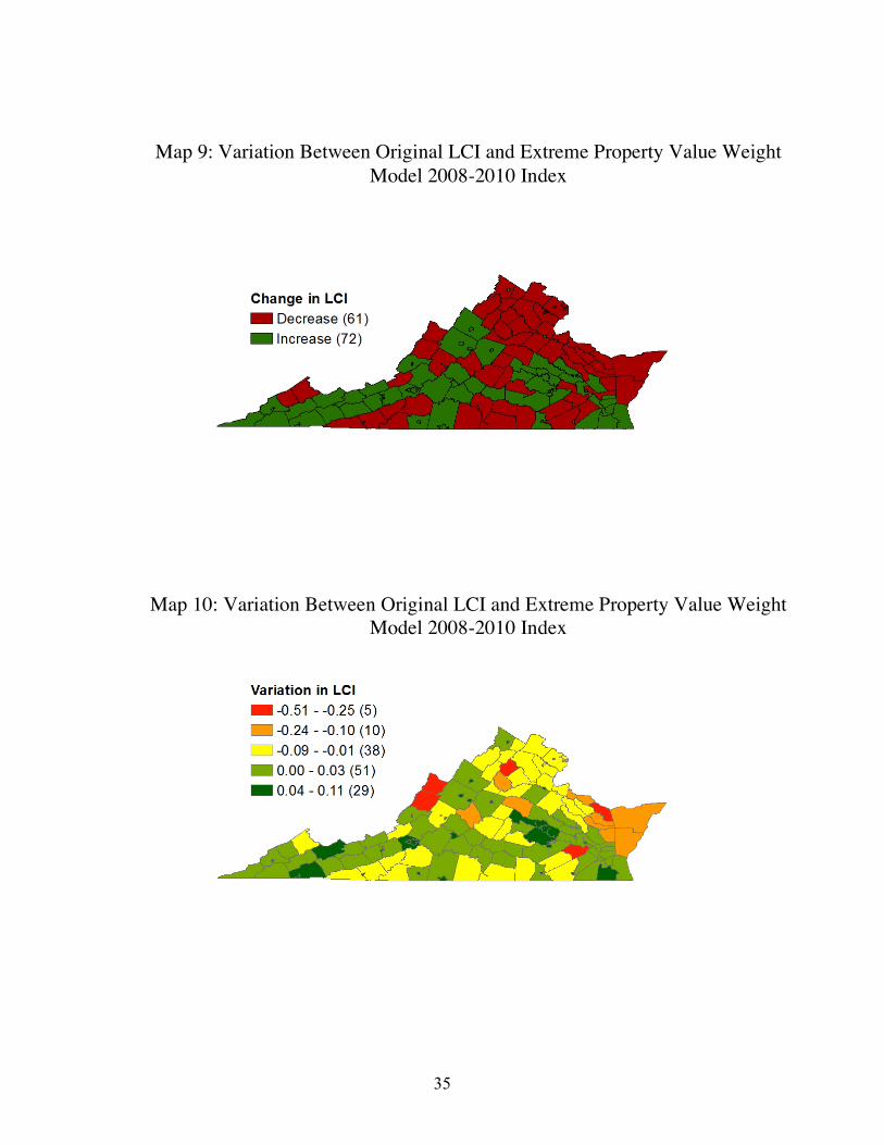
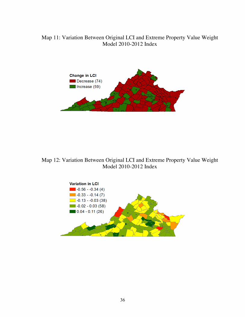
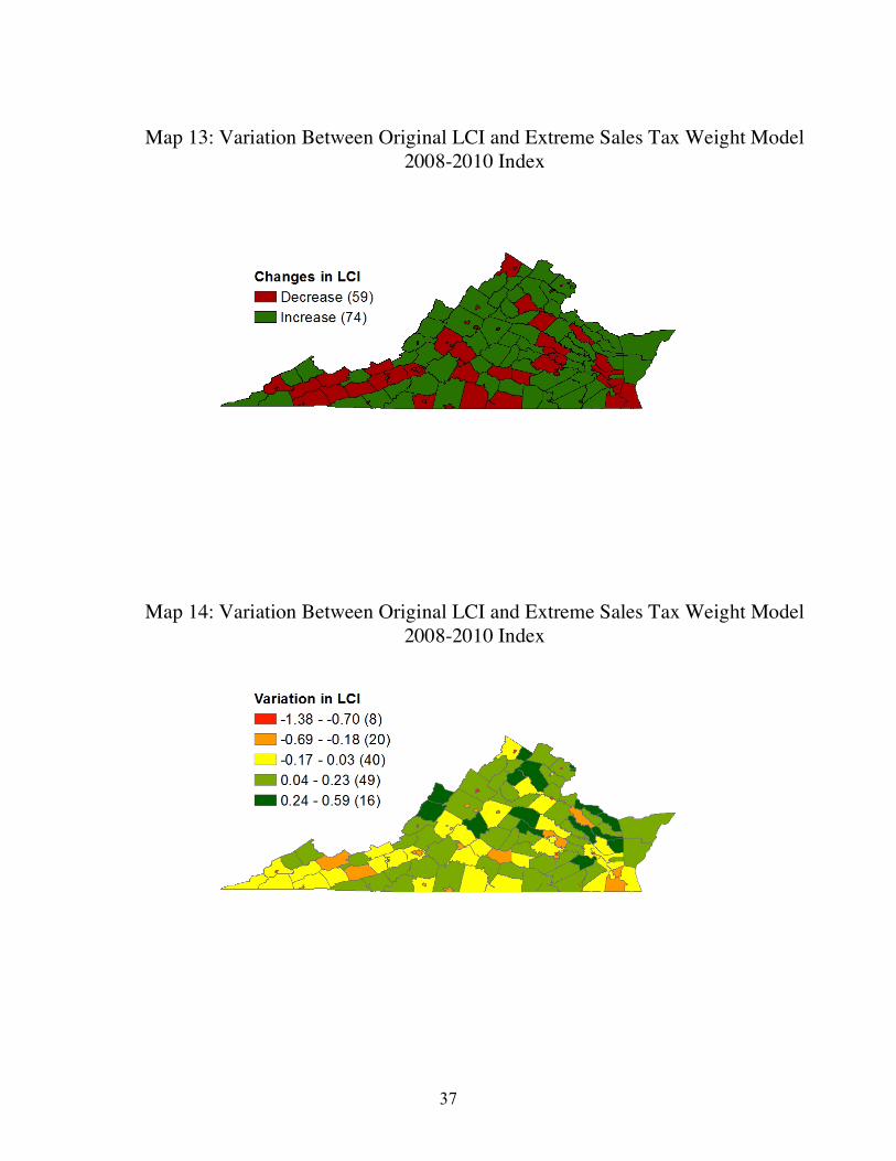
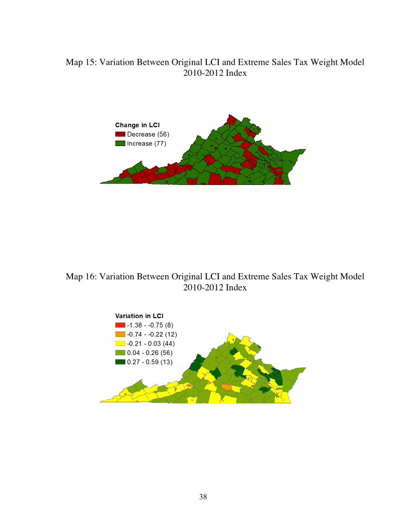
We illustrated the fairness issue by showing the effect of changing from original LCI to alternative models for each locality on the maps in Appendix 1. The maps of the sign of LCI change reveal that only the extreme sales tax model and the equivalent weighting models would consistently lead to more state funding for cities.11 A heat map confirmed that cities under the extreme sales tax and equal weight models gained the most funding.12 South-west Virginia, and more rural counties would consistently gain more state funding only under the equivalent weighting and extreme AGI models,13 otherwise those counties would actually see either changing funding or a decrease in funding. Areas around cities like Richmond would gain funding under every model but the extreme property value model.14 Maps of the magnitude of LCI change revealed that under the extreme AGI model, the Richmond area and some southwest localities would gain the most funding.15 Northern Virginia would see an increase in LCI score under the extreme property value model, however according to the heat map, they would not suffer as much of a funding loss as other counties would.16 Unsurprisingly, there was no significant difference in patterns between the extreme property value 2008-2010 index and the extreme property value 2010-2012 index in either the magnitude or the sign change maps. However, this suggests that the recovery has mainly been limited within counties, and is not reflected across large areas, since the variation of these models was very high across time periods.

Comparison of Variation Across Models Across Time Periods

We compared the distributions of raw value changes in the model from the 2008-2010 period to the 2010-2012 period (See Figure 5). The x-axis shows the raw value of change from the 2008-2010 index to the 2010-2012 index, found by subtracting the 2008-2010 index value from the 2010-2012 index value. The y-axis displays the number of localities that fall into a specific change. From Figure 5, we can see that extreme sales tax and extreme AGI models each have a relatively tall distribution and are both centered at around zero. However, although the extreme sales tax model has a high spike, it has a long tail, indicating that some localities have relatively large changes between the two time periods. In sum, for most localities, the extreme sales tax and extreme AGI models are stable across the two time periods even though some localities saw relatively larger changes under the extreme sales tax model.

The extreme property value model, however, is relatively dispersed, and is centered on a positive number. In fact, a majority of the distribution of the extreme property value model is on the positive side of the x-axis. This means that most localities have relatively large changes in true value of property from 2008-2010 index to the 2010-2012 index. This is expected because

11 See Appendix 1, maps 1-4 and 13-16. 12 See Appendix 1, maps 2, 4, 14 and 16. 13 See Appendix 1, maps 1-4, and 5-8. 14 See Appendix 1. 15 See Appendix 1, maps 5-8. 16 See Appendix 1, maps 9-12.

8

property values did recover after the 2008 financial crisis. This model confirms and reflects this recovery.

In the two indices of interest, measures of sales tax and AGI contribute to the stability for most localities, and the true value of property measure captures the effect of financial crisis and thus contributes to the variation. The current LCI model weighs true value of property at 50 percent, and its distribution is fatter and right skewed compared to the equal weights model, which weighs true value of property at 33 percent.

Figure 5: Index value variation between two periods, varying component weights

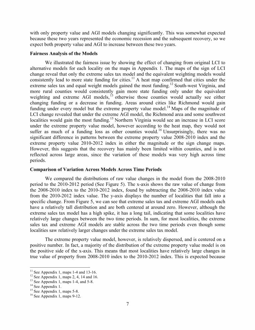
We further approximated the stability of different models by summing up the squared difference of the 136 localities’ between the two indices and taking square root of the sum. This is illustrated in Figure 6. The variation for the original LCI is 0.4582, for the extreme property model is 0.6765, for the extreme AGI model is 0.3601, for the extreme sales tax model is 0.6231, and for the equal weights model is 0.4169.

Because most values in the extreme property model are positive and the distribution is the relatively fat, the extreme property model has the highest variation between time periods. The relatively high variation in the extreme sales tax model is likely due to the extreme cases in its tails as well. The extreme AGI model has the lowest variation measure because its distribution is the thinnest, and because the tails of the distribution are relatively short.

Consistent with the distribution analysis, AGI contributes to the stability of the LCI measures, while property value contributes to the variation. The original LCI has the third lowest variation measure among the five. Its variation measure is higher than that of the equal weights model, because the current LCI weighs property value at 50 percent, while equal weights model weighs property value at 33 percent.

9

Figure 6: Sum of locality LCI variance between two time periods squared, varying component weights

In sum, in the time periods of interest, property value reflects the financial crisis because of the high variability across years. We recommend that policy makers pay attention to the possibility of external shocks, the vulnerability of the component variables to those external shocks, and the desired level of sensitively of the LCI to external shocks when updating the LCI.

Population Adjusted Models Comparison of Variation Across Models Within Time Periods

To begin, we analyzed the variation between the original LCI and our model LCI in the same way as for the component varied models.

10

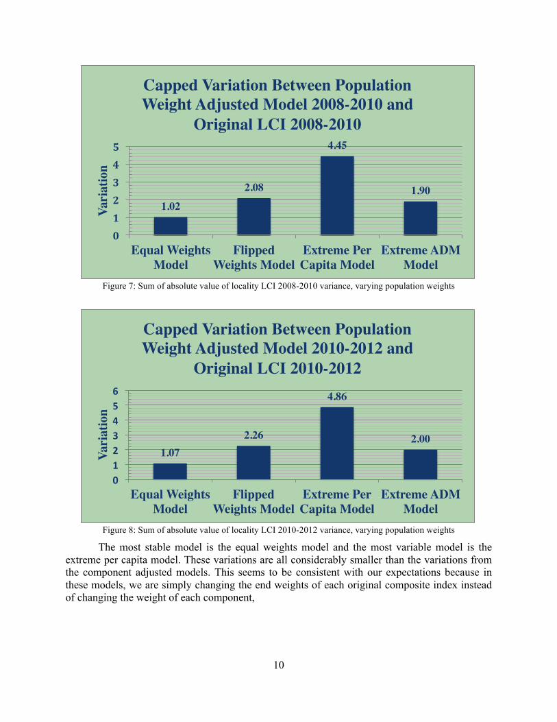
Figure 7: Sum of absolute value of locality LCI 2008-2010 variance, varying population weights

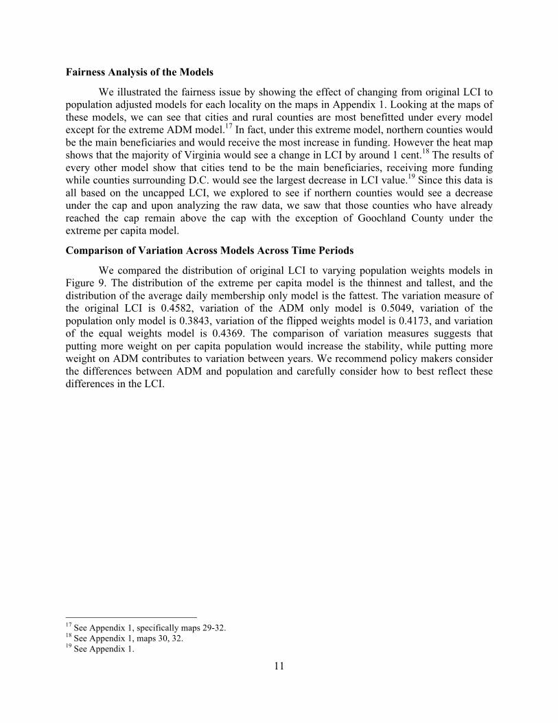
Figure 8: Sum of absolute value of locality LCI 2010-2012 variance, varying population weights

The most stable model is the equal weights model and the most variable model is the extreme per capita model. These variations are all considerably smaller than the variations from the component adjusted models. This seems to be consistent with our expectations because in these models, we are simply changing the end weights of each original composite index instead of changing the weight of each component,

1.022.08

4.45

1.90

012345

Equal Weights Model

Flipped Weights Model

Extreme Per Capita Model

Extreme ADM Model

Vari

atio

nCapped Variation Between Population Weight Adjusted Model 2008-2010 and


1.072.26

4.86

2.00

0123456

Equal Weights Model

Flipped Weights Model

Extreme Per Capita Model

Extreme ADM Model

Vari

atio

n

Capped Variation Between Population Weight Adjusted Model 2010-2012 and


11

Fairness Analysis of the Models

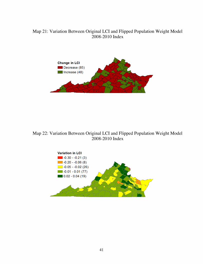
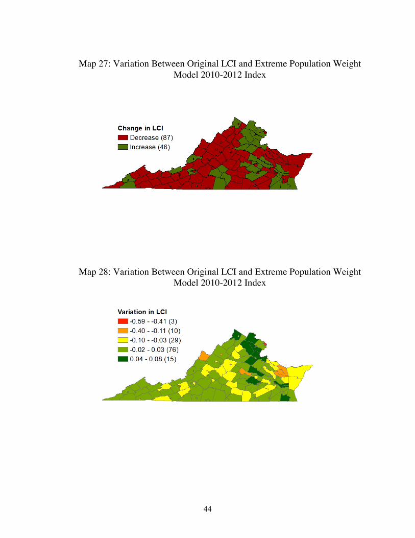
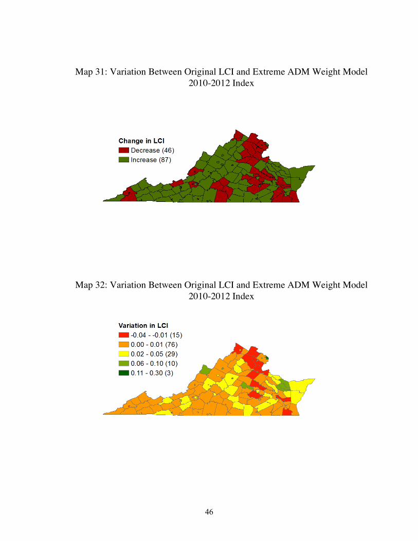
We illustrated the fairness issue by showing the effect of changing from original LCI to population adjusted models for each locality on the maps in Appendix 1. Looking at the maps of these models, we can see that cities and rural counties are most benefitted under every model except for the extreme ADM model.17 In fact, under this extreme model, northern counties would be the main beneficiaries and would receive the most increase in funding. However the heat map shows that the majority of Virginia would see a change in LCI by around 1 cent.18 The results of every other model show that cities tend to be the main beneficiaries, receiving more funding while counties surrounding D.C. would see the largest decrease in LCI value.19 Since this data is all based on the uncapped LCI, we explored to see if northern counties would see a decrease under the cap and upon analyzing the raw data, we saw that those counties who have already reached the cap remain above the cap with the exception of Goochland County under the extreme per capita model.

Comparison of Variation Across Models Across Time Periods

We compared the distribution of original LCI to varying population weights models in Figure 9. The distribution of the extreme per capita model is the thinnest and tallest, and the distribution of the average daily membership only model is the fattest. The variation measure of the original LCI is 0.4582, variation of the ADM only model is 0.5049, variation of the population only model is 0.3843, variation of the flipped weights model is 0.4173, and variation of the equal weights model is 0.4369. The comparison of variation measures suggests that putting more weight on per capita population would increase the stability, while putting more weight on ADM contributes to variation between years. We recommend policy makers consider the differences between ADM and population and carefully consider how to best reflect these differences in the LCI.

17 See Appendix 1, specifically maps 29-32. 18 See Appendix 1, maps 30, 32. 19 See Appendix 1.

12

Figure 9: Index value variation between two periods, varying population component weights

Figure 10: Sum of locality LCI variance between two time periods squared, varying population weights

05

1015

20Nu

mbe

r of L

ocali

ties

-.2 -.15 -.1 -.05 0 .05 .1 .15 .2Differences between Indices of Two Time Periods

Original ADM OnlyPopulation Only Flipped WeightsEqual Weights

Variation Between Time Periods, Different Combiantion of ADM and Population

.35

.4.4

5.5

Squa

re o

f sum

squr

ed ch

ange

value

Origina

l LCI

Extrem

e ADM

Extrem

e Per

Capita

Flipped

Weig

hts

Equal W

eights

Number

Variation of Index Value from 2008-2010 to 2010-2012

13

Section Conclusion We cannot firmly say which model, between the component and population models, is

the best model. However, we can say that the model that varies the least from the original LCI, in the two years we observed, appears to be the equal population weight model. Not only is the variation the smallest between the original model and the equal population weight model, there also seems to be an acceptable realignment of funds to cities and rural areas. This model also tends to not depress the LCI scores of many wealthy counties below the cap.

Even compared to the original model, the equal population weights model seems to be more stable across years. The extreme sales tax model varies from the original LCI most, and considering the lack of pattern to the redistribution of funding, we would strongly recommend against using this kind of model.

Additional Variables

There are demographic differences, different variations in income, differences in poverty density, and thus different budgetary constraints for each local school system. In an effort to control for these social differences and to observe their relationship to the LCI, we have run regression analyses to get at the heart of this relationship. We have included two other school district specific variables: students who receive free and reduced lunch and students with Limited English Proficiency (LEP). These variables are indicative of specific extra stresses on a locality’s budgets and resources. Furthermore, free and reduced lunch is an indicator of child poverty within the school age population for that locality. Since these students will need more resources than the average student for that district, their inclusion is meant to determine whether localities with high concentrations of students who receive free and reduced lunch and/or high concentrations of LEP students should receive more funds in order to provide these students with the resources needed to better meet the Standards of Quality.

Population density is an important indicator of urban development. Urban areas are more likely to have increased poverty, higher poverty density, and greater wealth. In addition, these areas deal with a large distribution in income across their populations. Thus it is likely that areas with high population density are associated with the need for more resources in order to properly serve their diverse populations. Previous JLARC reports have included population density as an explanatory in their models and with success.20 Therefore, we feel it prudent to include population density as well to verify if that variable increases explanatory power with more current data.

Regression Analysis Data and Methodology

We compiled much of our demographic data from the U.S. Census Bureau, specifically, from the American Fact Finder’s 2010 5-year American Community Survey estimates. We believe these estimates to be the most accurate available data. However, data was also sourced from the Virginia Department of Education, from the Commission on Local Government, and

20 Ibid, 130.

14

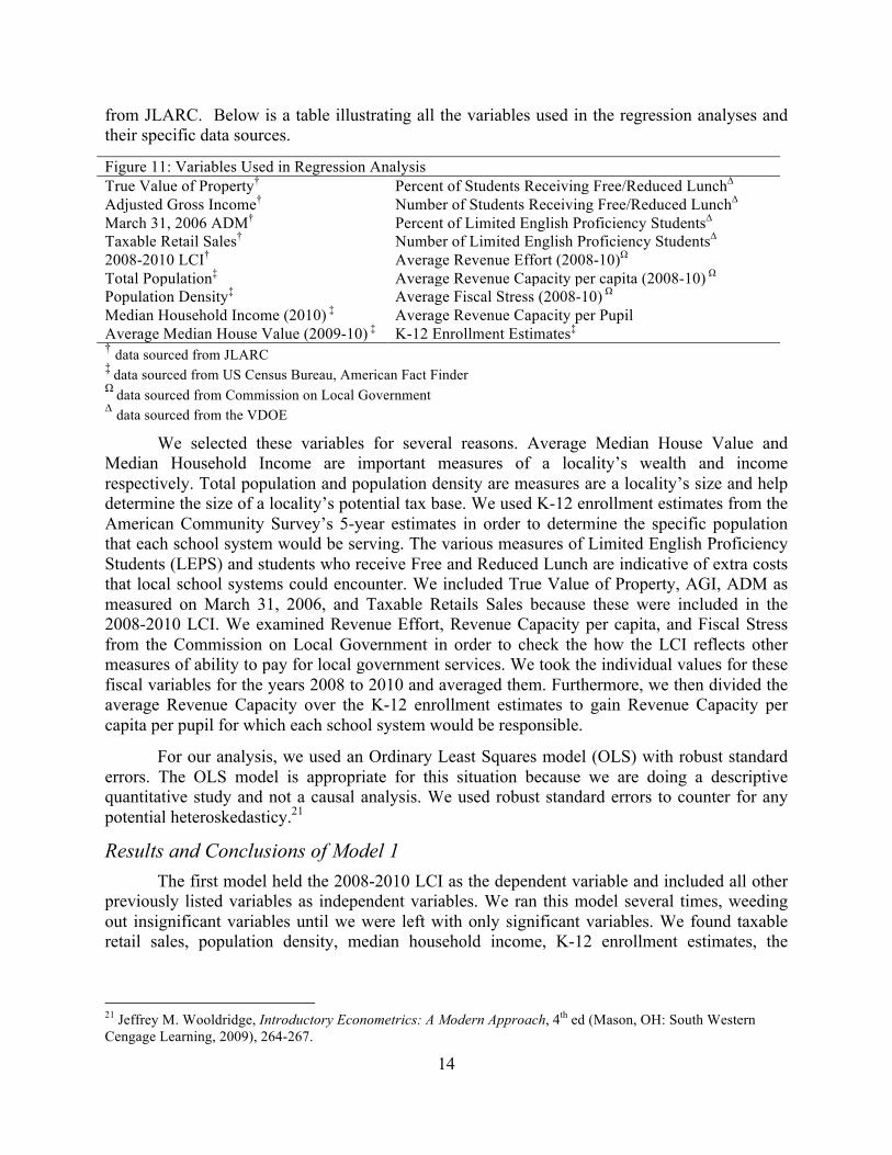
from JLARC. Below is a table illustrating all the variables used in the regression analyses and their specific data sources.

Figure 11: Variables Used in Regression Analysis True Value of Property† Percent of Students Receiving Free/Reduced Lunch∆

Adjusted Gross Income† Number of Students Receiving Free/Reduced Lunch∆ March 31, 2006 ADM† Percent of Limited English Proficiency Students∆ Taxable Retail Sales† Number of Limited English Proficiency Students∆ 2008-2010 LCI† Average Revenue Effort (2008-10)Ω

Total Population‡ Average Revenue Capacity per capita (2008-10) Ω Population Density‡ Average Fiscal Stress (2008-10) Ω Median Household Income (2010) ‡ Average Revenue Capacity per Pupil Average Median House Value (2009-10) ‡ K-12 Enrollment Estimates‡ † data sourced from JLARC ‡ data sourced from US Census Bureau, American Fact Finder Ω data sourced from Commission on Local Government ∆ data sourced from the VDOE

We selected these variables for several reasons. Average Median House Value and Median Household Income are important measures of a locality’s wealth and income respectively. Total population and population density are measures are a locality’s size and help determine the size of a locality’s potential tax base. We used K-12 enrollment estimates from the American Community Survey’s 5-year estimates in order to determine the specific population that each school system would be serving. The various measures of Limited English Proficiency Students (LEPS) and students who receive Free and Reduced Lunch are indicative of extra costs that local school systems could encounter. We included True Value of Property, AGI, ADM as measured on March 31, 2006, and Taxable Retails Sales because these were included in the 2008-2010 LCI. We examined Revenue Effort, Revenue Capacity per capita, and Fiscal Stress from the Commission on Local Government in order to check the how the LCI reflects other measures of ability to pay for local government services. We took the individual values for these fiscal variables for the years 2008 to 2010 and averaged them. Furthermore, we then divided the average Revenue Capacity over the K-12 enrollment estimates to gain Revenue Capacity per capita per pupil for which each school system would be responsible.

For our analysis, we used an Ordinary Least Squares model (OLS) with robust standard errors. The OLS model is appropriate for this situation because we are doing a descriptive quantitative study and not a causal analysis. We used robust standard errors to counter for any potential heteroskedasticy.21

Results and Conclusions of Model 1 The first model held the 2008-2010 LCI as the dependent variable and included all other previously listed variables as independent variables. We ran this model several times, weeding out insignificant variables until we were left with only significant variables. We found taxable retail sales, population density, median household income, K-12 enrollment estimates, the

21 Jeffrey M. Wooldridge, Introductory Econometrics: A Modern Approach, 4th ed (Mason, OH: South Western Cengage Learning, 2009), 264-267.

15

number of LEP students, average Revenue Capacity per capita, and the average median house value to be significant.

Figure 12: Regression Analysis Results from Model 1 Variable Coefficient T-Statistic

Taxable Retail Sales 6.98e-11*** 3.98 Population Density -1.42e-5* -2.49 Median Household Income -4.64e-6*** -4.91

K-12 Enrollment Estimates -4.20e-6*** -4.06 LEPS 3.47e-6† 1.76 AVG Revenue Capacity 1.66e-4*** 12.83 AVG Median House Value 1.06e-6*** 5.2 constant 0.118*** 4.93 R2 0.923 Adjusted R2 0.919 p<0.1†, * p<0.05, ** p<0.01, *** p<0.001

These coefficients are extremely small because very small changes in our dependent variable, LCI, translate to significant changes in funding for localities. Therefore, we sought to interpret these numbers with more practical lens. We found that a $10 million increase in taxable retail sales is associated with roughly a 0.0007 unit increase in the LCI. For population density, an increase in 1000 people per square mile is associated with a 0.0142 decrease in the LCI. A $1,000 increase in the median household income is associated with approximately a 0.005 unit decrease in the LCI. It is important to note that when we control for other variables, the LCI does not behave the way we would want it to in regards to an increase in the median household income. We also found that every extra 100 students estimated to enroll in a locality’s public schools is associated with a 0.0004 unit decrease in the LCI. A 100 person increase in the population of Limited English Proficiency Students in a locality’s public school system is associated with a 0.000347 unit increase in the LCI. We also found that a $100 increase in a locality’s Average Revenue Capacity per capita is associated with a 0.0166 unit increase in the LCI. Finally, a $10,000 increase in average median house value for a locality is associated with a 0.0106 unit increase in the LCI. Model 1 has an R2 of 0.923, which means that this model accounts for approximately 92% of the variation in the 2008-2010 LCI. In other words, Model 1 will predict roughly 92% of the variation in the LCI. Overall, the LCI appears to be an adequate measure of ability to pay for local school systems.

An Alternate Measure of Ability to Pay Based on our map analysis of the Commission on Local Government’s fiscal measures, we decided to test Revenue Capacity per capita as an alternate measure of ability to pay. Revenue Capacity per capita is often used by local governments and other agencies to determine

16

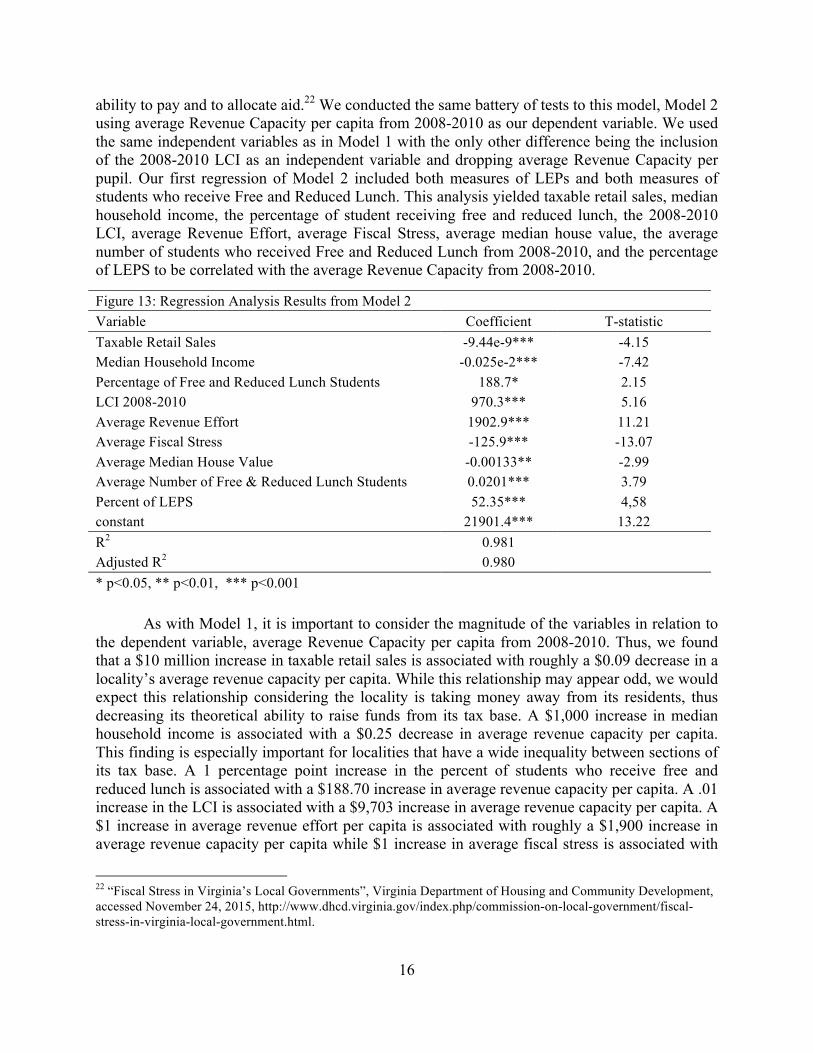
ability to pay and to allocate aid.22 We conducted the same battery of tests to this model, Model 2 using average Revenue Capacity per capita from 2008-2010 as our dependent variable. We used the same independent variables as in Model 1 with the only other difference being the inclusion of the 2008-2010 LCI as an independent variable and dropping average Revenue Capacity per pupil. Our first regression of Model 2 included both measures of LEPs and both measures of students who receive Free and Reduced Lunch. This analysis yielded taxable retail sales, median household income, the percentage of student receiving free and reduced lunch, the 2008-2010 LCI, average Revenue Effort, average Fiscal Stress, average median house value, the average number of students who received Free and Reduced Lunch from 2008-2010, and the percentage of LEPS to be correlated with the average Revenue Capacity from 2008-2010.

As with Model 1, it is important to consider the magnitude of the variables in relation to the dependent variable, average Revenue Capacity per capita from 2008-2010. Thus, we found that a $10 million increase in taxable retail sales is associated with roughly a $0.09 decrease in a locality’s average revenue capacity per capita. While this relationship may appear odd, we would expect this relationship considering the locality is taking money away from its residents, thus decreasing its theoretical ability to raise funds from its tax base. A $1,000 increase in median household income is associated with a $0.25 decrease in average revenue capacity per capita. This finding is especially important for localities that have a wide inequality between sections of its tax base. A 1 percentage point increase in the percent of students who receive free and reduced lunch is associated with a $188.70 increase in average revenue capacity per capita. A .01 increase in the LCI is associated with a $9,703 increase in average revenue capacity per capita. A $1 increase in average revenue effort per capita is associated with roughly a $1,900 increase in average revenue capacity per capita while $1 increase in average fiscal stress is associated with

22 “Fiscal Stress in Virginia’s Local Governments”, Virginia Department of Housing and Community Development, accessed November 24, 2015, http://www.dhcd.virginia.gov/index.php/commission-on-local-government/fiscal-stress-in-virginia-local-government.html.

Figure 13: Regression Analysis Results from Model 2 Variable Coefficient T-statistic Taxable Retail Sales -9.44e-9*** -4.15 Median Household Income -0.025e-2*** -7.42 Percentage of Free and Reduced Lunch Students 188.7* 2.15 LCI 2008-2010 970.3*** 5.16 Average Revenue Effort 1902.9*** 11.21 Average Fiscal Stress -125.9*** -13.07 Average Median House Value -0.00133** -2.99 Average Number of Free & Reduced Lunch Students 0.0201*** 3.79 Percent of LEPS 52.35*** 4,58 constant 21901.4*** 13.22 R2 0.981 Adjusted R2 0.980 * p<0.05, ** p<0.01, *** p<0.001

17

approximately a $126 decrease in average revenue capacity per capita. We also found that a $10,000 increase in the median house values is associated with a $13.30 decrease in revenue capacity. While this relationship may appear counterintuitive, a high median house value often equates to higher house payments, thus impacting a family’s disposable income and its ability to contribute more taxes to the state. However, average median house value is a proxy for wealth and so it is just as likely that people who can afford high house payments will be able to afford a modest tax increase as well. We found that a 100 person increase in the number of students who receive free and reduced lunch is associated with a $2 increase in average revenue capacity per capita. Finally, we found that a 1 percentage point increase in LEP students is associated with a $52.35 increase in average revenue capacity per capita.

Essentially, Revenue Capacity per capita is associated with more factors that we believe are important to determining a locality’s ability to pay for its school system. Furthermore, Model 2 has an R2 of 0.981 which means that this model accounts for roughly 98% of the variation in average Revenue Capacity per capita. Thus, revenue capacity per capita is more likely to reflect changes in demographics and general trends in the economy that would impact a locality’s ability to pay more effectively than the LCI.

Ranking Analysis The LCI is intended to capture the fiscal aspects of localities’ ability to pay and therefore should track the corresponding fiscal measure of the localities. We compared LCI with fiscal measures – revenue capacity, fiscal effort, and fiscal stress -- developed by Commission on Local Government (CLG fiscal measures).23 Revenue capacity is a per capita measure that measures the theoretical ability of a locality to generate revenue, which takes into consideration of each locality’s specific tax base and current ability to raise revenue. 24 Revenue effort is the amount of theoretical revenue capacity per capita that the locality actually collects through taxes and fees. Fiscal stress measures the locality’s fiscal ability to respond to economic shocks, taking into consideration revenue capacity per capita, revenue effort, and median household income.

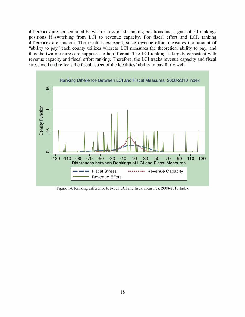
Ranking disparity between LCI and Fiscal Measures Figures 14 and 15 plot the differences between localities’ fiscal measures rankings and LCI rankings for the two indices of interest, 2008-2010 and 2010-2012, respectively. The x-axis is the value obtained by subtracting a locality’s ranking in a fiscal measure from its ranking in the LCI. This difference indicates the gain or loss of ranking position by switching from LCI measures to fiscal measures. In other words, a positive value on the x-axis indicates that the locality’s ability to pay is high on the LCI, but low on the fiscal measures, while a negative value on the x-axis means that the locality’s ability to pay is low on the LCI, but high on the fiscal measures. The y-axis is the percentage of the localities.

Figure 14 and Figure 15 show that for revenue capacity and LCI, most ranking differences are concentrated between a loss of 30 ranking positions and a gain of 30 ranking positions if switching from LCI to revenue capacity. For fiscal stress and LCI, most ranking

23 About Commission for Local Government, http://www.dhcd.virginia.gov/index.php/commission-on-local-government.html. 24 Fiscal Stress in Virginia Local Government, http://www.dhcd.virginia.gov/index.php/commission-on-local-government/fiscal-stress-in-virginia-local-government.html

18

differences are concentrated between a loss of 30 ranking positions and a gain of 50 rankings positions if switching from LCI to revenue capacity. For fiscal effort and LCI, ranking differences are random. The result is expected, since revenue effort measures the amount of “ability to pay” each county utilizes whereas LCI measures the theoretical ability to pay, and thus the two measures are supposed to be different. The LCI ranking is largely consistent with revenue capacity and fiscal effort ranking. Therefore, the LCI tracks revenue capacity and fiscal stress well and reflects the fiscal aspect of the localities’ ability to pay fairly well.

Figure 14: Ranking difference between LCI and fiscal measures, 2008-2010 Index

0.0

5.1

.15

Dens

ity F

uncti

on

-130 -110 -90 -70 -50 -30 -10 10 30 50 70 90 110 130Differences between Rankings of LCI and Fiscal Measures

Fiscal Stress Revenue CapacityRevenue Effort

Ranking Difference Between LCI and Fiscal Measures, 2008-2010 Index

19

Figure 15: Ranking difference between LCI and fiscal measures, 2010-2012 Index

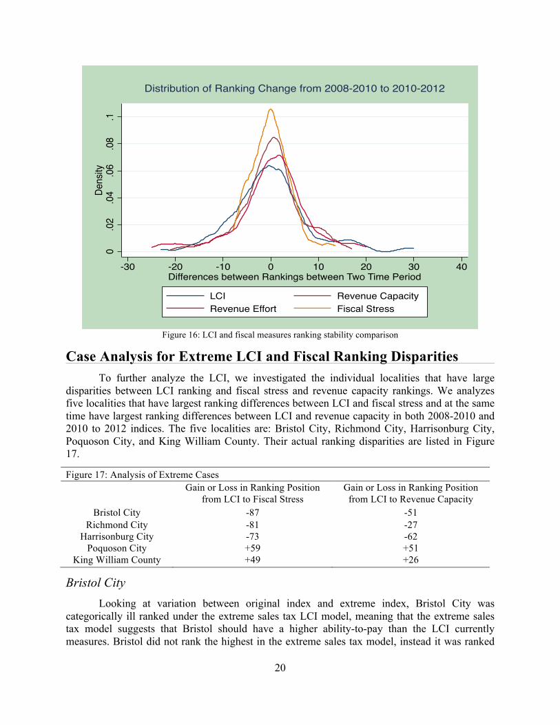
Ranking stability between 2008-2010 Indices and 2010-2012 Indices for LCI and Fiscal Measures We also analyzed the stability aspects of the LCI compared to fiscal measures. Figure 16 plots the distribution of raw value changes in counties between the LCI and fiscal measures. We can see that fiscal stress has the highest spike and thinnest tail; therefore, it is the most stable measure. All fiscal measures are taller and thinner than LCI, and have shorter and thinner tails than LCI. However, revenue effort and fiscal stress have fatter tails on the left end of the spectrum.

In general, for most localities, the ranking change between the two time periods of interest is smaller in fiscal measures than in the LCI. Fiscal stress is the most stable measure in terms of ranking, followed by revenue capacity and revenue effort. There are a few localities that have larger ranking improvements from 2008-2010 to 2010-2012 in fiscal stress and revenue capacity measures than in LCI measures.

It is worth noting that the ranking change analysis of LCI does not show the whole picture of the LCI’s stability. The LCI is capped at 0.8, but the ranking of LCI is variable above 0.8 because we used the uncapped LCI in the ranking measure. Therefore, counties may have a raw LCI above 0.8 and even though their LCI ranking may change, their actual LCI is stuck at 0.8 and does not change.

20

Figure 16: LCI and fiscal measures ranking stability comparison

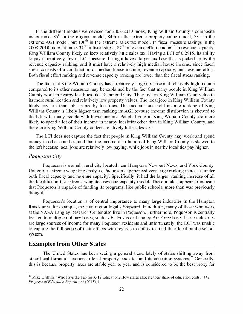
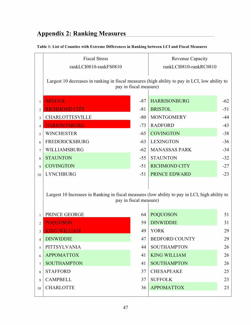
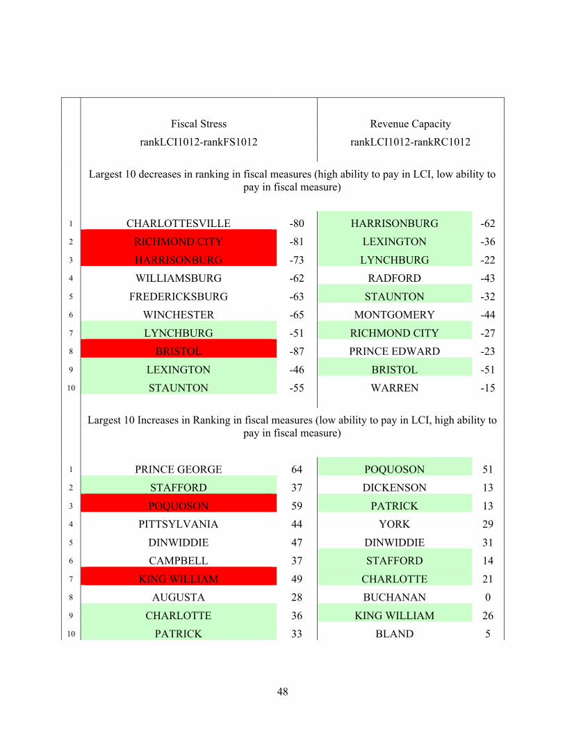
Case Analysis for Extreme LCI and Fiscal Ranking Disparities To further analyze the LCI, we investigated the individual localities that have large disparities between LCI ranking and fiscal stress and revenue capacity rankings. We analyzes five localities that have largest ranking differences between LCI and fiscal stress and at the same time have largest ranking differences between LCI and revenue capacity in both 2008-2010 and 2010 to 2012 indices. The five localities are: Bristol City, Richmond City, Harrisonburg City, Poquoson City, and King William County. Their actual ranking disparities are listed in Figure 17.

Figure 17: Analysis of Extreme Cases Gain or Loss in Ranking Position

from LCI to Fiscal Stress Gain or Loss in Ranking Position from LCI to Revenue Capacity

Bristol City -87 -51 Richmond City -81 -27

Harrisonburg City -73 -62 Poquoson City +59 +51

King William County +49 +26

Bristol City Looking at variation between original index and extreme index, Bristol City was

categorically ill ranked under the extreme sales tax LCI model, meaning that the extreme sales tax model suggests that Bristol should have a higher ability-to-pay than the LCI currently measures. Bristol did not rank the highest in the extreme sales tax model, instead it was ranked

0.0

2.0

4.0

6.0

8.1

Dens

ity

-30 -20 -10 0 10 20 30 40Differences between Rankings between Two Time Period

LCI Revenue CapacityRevenue Effort Fiscal Stress

Distribution of Ranking Change from 2008-2010 to 2010-2012

21

as number 15 in the 2008-2010 index and number 10 in the 2008-2010 index. Some of the reason why Bristol is labeled as an extreme may be due to the difference between the original LCI and the model LCI. To explore this possibility, we created a ratio of the original index to the model index. This showed that Bristol City’s ratio is actually comparatively low and ranks as number 21 in 2008, and number 10 in 2010. Even looking at the raw values of sales tax and the sales tax per ADM, we see that Bristol City is not an exceptional case.

One reason that sales tax may be impacting Bristol City so extremely is that their twin city in Tennessee is the location of a large NASCAR stadium. While the stadium is located down the interstate from Bristol, VA, it would not be impossible for customers to stay in Virginia hotels and drive to the stadium. We believe that this large tourist attraction is the reason for the extreme mislabeling of Bristol City in the original LCI.

Harrisonburg City Harrisonburg City is also highlighted under the extreme sales tax model as a locality that may have a higher ability to pay than the original LCI determines. This new index shows that Harrisonburg City is ranked in the top 10 under the extreme sales tax LCI. Again we analyzed whether this was due to a high original LCI and determined that the ratio is very low and that there is an extreme difference between the new LCI and the original. In fact, the extreme sales tax LCI bumps Harrisonburg well above the 0.8 cap. Harrisonburg also does not have a very large ratio of raw sales tax per ADM.

One possibility for this extreme case is that Harrisonburg City is the home of James Madison University and is the county seat of Rockbridge County. Because of the large university located within its boundaries, we would assume that there are many sports fans, parents, professors, students, and visiting guests spending money within the city and contributing to a robust sales tax base. Although Harrisonburg may have a large tax base, this is not reflected in the current weighting of the LCI, thus why there is such a difference between the original LCI and the model LCI.

Richmond City Richmond city is highlighted under the extreme sales tax model much like the other cities

we analyzed. Richmond did not have the highest sales tax LCI ranking, nor did it have the largest ratio of original LCI to sales tax LCI. In fact, Richmond City has a ratio of .78 and is on of the highest we chose to evaluate. The raw data for sales tax as well as the sales tax per ADM ratio were not the largest either.

What we have guessed is the cause of the disparity between original LCI and the model LCI, is that, since Richmond is the state capital, there is significant tourism that drives sales tax and causes the apparent disparity.

King William County In both the 2008-2010 index and the 2008-2010 index, King William County’s LCI ranking

is 49 spaces lower than its fiscal stress ranking, and 26 spaces lower than its revenue capacity ranking. It has low ability to pay in LCI, and high ability to pay in fiscal measures.

22

In the different models we devised for 2008-2010 index, King William County’s composite index ranks 85th in the original model, 84th in the extreme property value model, 78th in the extreme AGI model, but 106th in the extreme sales tax model. In fiscal measure rakings in the 2008-2010 index, it ranks 37th in fiscal stress, 87th in revenue effort, and 60th in revenue capacity. King William County likely collects relatively little sales tax. Having a LCI of 0.2915, its ability to pay is relatively low in LCI measure. It might have a larger tax base that is picked up by the revenue capacity ranking, and it must have a relatively high median house income, since fiscal stress consists of a combination of median house income, revenue capacity, and revenue effort. Both fiscal effort ranking and revenue capacity ranking are lower than the fiscal stress ranking.

The fact that King William County has a relatively large tax base and relatively high income compared to its other measures may be explained by the fact that many people in King William County work in nearby localities like Richmond City. They live in King William County due to its more rural location and relatively low property values. The local jobs in King William County likely pay less than jobs in nearby localities. The median household income ranking of King William County is likely higher than ranking its AGI because income distribution is skewed to the left with many people with lower income. People living in King William County are more likely to spend a lot of their income in nearby localities other than in King William County, and therefore King William County collects relatively little sales tax.

The LCI does not capture the fact that people in King William County may work and spend money in other counties, and that the income distribution of King William County is skewed to the left because local jobs are relatively low paying, while jobs in nearby localities pay higher.

Poquoson City Poquoson is a small, rural city located near Hampton, Newport News, and York County. Under our extreme weighting analysis, Poquoson experienced very large ranking increases under both fiscal capacity and revenue capacity. Specifically, it had the largest ranking increase of all the localities in the extreme weighted revenue capacity model. These models appear to indicate that Poquoson is capable of funding its programs, like public schools, more than was previously thought.

Poquoson’s location is of central importance to many large industries in the Hampton Roads area, for example, the Huntington Ingalls Shipyard. In addition, many of those who work at the NASA Langley Research Center also live in Poquoson. Furthermore, Poquoson is centrally located to multiple military bases, such as Ft. Eustis or Langley Air Force base. These industries are large sources of income for many Poquoson residents and unfortunately, the LCI was unable to capture the full scope of their effects with regards to ability to fund their local public school system.

Examples from Other States The United States has been seeing a general trend lately of states shifting away from

other local forms of taxation to local property taxes to fund its education systems.25 Generally, this is because property taxes are stable year to year and is considered to be the best proxy for

25 Mike Griffith, “Who Pays the Tab for K-12 Education? How states allocate their share of education costs,” The Progress of Education Reform, 14: (2013), 1.

23

wealth of a community.26 There are only two states that do not base the cost of education on relative wealth or ability to pay; these states are Pennsylvania and Hawaii.27

We have chosen to conduct a summary literature review of how Maryland and Georgia distribute their educational funding. We chose these two states because they were similar to Virginia in that they both have large metropolitan cities and a disparity between rural and urban counties. We have also chosen these states because Maryland measures ability to pay using a mixture of many different components, much like Virginia, whereas Georgia only measures ability to pay through property value.28 The common thread through all of this is that there is a serious question in many states whether the distribution of funds according to property taxes is fair and sustainable. In fact, there have been lawsuits filed against states because of the inequality perceived in the distribution of education funds via a property tax system.29 Although this is an interesting point to note, these cases have only been tried in state court and not on the federal level, so there is no actual precedent between states.

Maryland creates a Standard of Quality measure for education by which the state obtains a base cost per pupil, makes adjustments for any at risk populations, and adjusts for differences in local cost of educational resources.30 The ability to pay measure for Maryland is found using the following formula: (Total real property values x 0.4) + (total personal property x 0.5) + (public utilities’ assessable base) + (net taxable income) = total district wealth.31 It is unclear how each of these pieces is calculated due to a general lack of transparency in Maryland’s education funding scheme. Each locality sets its own taxes on income, so taxes are widely varied from county to county, reaching anywhere from one percent to three percent.32 Public utilities’ assessable base is described as the “assessed value of the operating real property of public utilities” however we were unable to find exactly how this piece of the equation is calculated.33 The major problem we ran into while assessing Maryland’s ability to pay structure is a total lack of transparency in the calculation of their index. It was unclear exactly how each piece is calculated and it was unclear how these pieces compare to Virginia’s LCI. We did find a consensus that adding in additional measures of income tends to lead to a more equitable distribution of education funding. In order to completely compare Maryland and Virginia’s ability to pay formulas, we would want to do a test comparing fiscal rankings of Maryland localities and Maryland’s funding rankings. This was not feasible in our time frame. We can only conclude that Maryland tends to be successful at measuring ability to pay and that they use a formula similar to the LCI but substitutes public utilities’ assessment for sales tax, however especially given that there is a general lack of transparency around the calculation of Maryland’s

26 Griffith, “Who Pays the Tab for K-12 Education?,” 1. 27 Ibid, 2. 28 Ibid, 3. 29 Thomas Thro, “The Third Wave: The Impact of the Montana, Kentucky, and Texas Decisions on the Future of Public School Finance Reform Litigation”, HeinOnline (1990), 234. 30 “Education in Maryland”, Department of Legislative Services, November 2014.,October 22, 2015. 31 W. Glenn et al, (2015). Analysis of School Finance Equity and Local Wealth Measures in Maryland. Denver, CO: Augenblick, Palaich & Associates, 32. 32 Ibid, 29. 33 Benjamin Scafidi, The Formula Behind Maryland’s K-12 Funding, Indianapolis: Friedman Foundation, 2008, Accessed November 15, 2015, http://files.eric.ed.gov/fulltext/ED508459.pdf, 10.

24

ability to pay, we are not able to conclusively say whether Virginia could gain from reformulating the LCI to match Maryland.

Georgia has been suffering severe budget cuts recently34 and many constituents are very unhappy as the cuts seem to have more of an impact on the poorer districts.35 Georgia’s K-12 public education system is funded only through property taxes. Georgia does not add on any additional measures, such as income tax, to their ability to pay formula. Although Georgia does collect income taxes, none of this money goes towards the education funding system. Localities do have the option to raise sales taxes by one percent to fund “special” education; however this additional money seems to be reserved.36 Localities pay for education funding through what is called the “fair share” of funding. The “fair share” is assessed through a comparison of the “dollar value of property sold during a given period of time to the value attached to the property by the local taxing agency”. This ratio is then compared to “the assessed value of property not sold to its appraised value as determined by the state agency”.37 State share of education funding is then found by comparing the entitlement of the locality and the localities fair share of funding.38 The entitlement of each locality is found by weighting the base cost of educating a 9-12 student in Georgia to the number of equivalent full time students in a locality. This system is generally regarded as not successful simply because property value is often not seen as a fair measure of ability to pay. Additionally, this system also does not seem to weight the cost of educating a student by locality, meaning that there is either under or over estimation of the cost of education in certain districts. On top of these issues, there are significant issues of whether property value accurately measures ability to pay. In order to further study this issue and compare Georgia’s method to that of Virginia, we would again want to compare fiscal rankings to funding rankings which was not feasible given our time and data constraints.

We conclude that, on the whole, states that add in additional measures of wealth or income tend to be better at measuring ability to pay. These states also seem to be facing fewer issues regarding perceived fairness in measuring ability to pay. Since Virginia has such a transparent, albeit complicated, formula, it seems to be better off than others.

Conclusion In light of our analysis, we think the original LCI does a good job at reflecting the

ability to pay of localities, and it tracks fiscal stress and revenue capacity fairly well. However, fiscal ranking measures may do a better job at capturing locality specific characteristics like number of minority population. We recommend taking into consideration and analyzing of fiscal measures further before updating the current LCI. We also recommend attempting to balance the economic reflectiveness of LCI with its components and the desirable level of stability necessary for budgeting purposes.

34 Claire Suggs, “Overview: 2016 Fiscal Year Budget for K-12 Education”, Georgia Budget & Policy Institute, January 2015, Accessed October 23, 2015, 3. 35 Nancy Badertscher, “Deal’s statement on education funding missing critical context,” PolitiFact Georgia, April 14th, 2015, Accessed October 15th, 2015, http://www.politifact.com/georgia/statements/2015/apr/14/nathan-deal/deals-statement-education-funding-missing-critical/ 36 Catherine Sielke, Georgia, Washington, DC: National Center for Education Statistics, 1999, Accessed November 15, 2015, https://nces.ed.gov/edfin/pdf/StFinance/Georgia.pdf, 3. 37 Ibid, 6. 38 Ibid, 5-7.

25

Bibliography Badertscher, Nancy. “Deal’s statement on education funding missing critical context”.

PolitiFact Georgia, April 14th, 2015. Accessed October 15th, 2015. http://www.politifact.com/georgia/statements/2015/apr/14/nathan-deal/deals-statement-education-funding-missing-critical/

Bosher, Bill. “Explaining the Local Composite Index”, NBC12, Feb.24, 2010.

http://www.nbc12.com/story/12038576/explaining-the-local-composite-index. Brooks, Gracie Hart. “School Funding Formula Complex”, Orange County Review,

February 6, 2014. http://www.dailyprogress.com/orangenews/news/school-funding-formula-complex/article_d35e5642-8f75-11e3-b51a-001a4bcf6878.html.

“Education in Maryland”. Department of Legislative Services. November 2014. October

22, 2015. http://mgaleg.maryland.gov/Pubs/LegisLegal/2014-legislativehandbook series-vol-9.pdf.

Glenn, W. J., Griffith, M., Picus, L.O., Odden, A. (2015). Analysis of School Finance

Equity and Local Wealth Measures in Maryland. Denver, CO: Augenblick, Palaich & Associates

Griffith, Mike. “Who Pays the Tab for K-12 Education? How states allocate their share of

education costs”. The Progress of Education Reform, 14: (2013), 1-7. Joint Legislative Audit and Review Commission of the Virginia General Assembly, “A

Review of Elementary and Secondary School Funding”, 2002. Moomaw, Graham. “City officials ask state lawmakers for help.” Richmond Times

Dispatch, November 7th, 2014. Accessed December 7th, 2015. http://m.richmond.com/article_f3d51741-4227-5233-9748-818c8cfe7324.html?mode=jqm

Scafidi, Benjamin. The Formula Behind Maryland’s K-12 Funding. Indianapolis:

Friedman Foundation, 2008. Accessed November 15, 2015. http://files.eric.ed.gov/fulltext/ED508459.pdf.

Sielke, Catherine. Georgia. Washington, DC: National Center for Education Statistics,

1999. Accessed November 15, 2015. https://nces.ed.gov/edfin/pdf/StFinance/ Georgia.pdf.

Suggs, Claire. “Overview: 2016 Fiscal Year Budget for K-12 Education”. Georgia Budget & Policy Institute. January 2015. October 23, 2015.

26

“The Basics of Georgia School Finance”. George School Council Institute. October 22, 2015.http://www.gsci.org/documents/Basics%20of%20GA%20School%20Finance_2007.pdf.

Thro, William E. “The Third Wave: The Impact of the Montana, Kentucky, and Texas

Decisions on the Future of Public School Finance Reform Litigation”. HeinOnline. 1990. October 20, 2015. http://home.heinonline.org/

Virginia Department of Housing and Community Development. “About Commission on

Local Government.” Accessed October 10th, 2015. http://www.dhcd.virginia.gov /index.php/commission-on-local-government.html.

Virginia Education Association, Inc., “Virginia’s Education Disparities FY 2008-09”.

Accessed October 29, 2015. http://www.veanea.org/assets/document/disparity-2010-07b.pdf.

Wooldridge, Jeffrey M. Introductory Econometrics: A Modern Approach, 4th ed, Mason,

OH: South Western Cengage Learning, 2009.

27

Appendix 1: Maps

31

Map 1: Variation Between Original LCI and Equal Component Weighting Model 2008-2010 Index


32



33

Map 5: Variation Between Original LCI and Extreme AGI Weight Model 2008-2010 Index


34



35

Map 9: Variation Between Original LCI and Extreme Property Value Weight Model 2008-2010 Index


36



37

Map 13: Variation Between Original LCI and Extreme Sales Tax Weight Model 2008-2010 Index


38



39

Map 17: Variation Between Original LCI and Equal Population Weight Model 2008-2010 Index


40



41

Map 21: Variation Between Original LCI and Flipped Population Weight Model 2008-2010 Index


42



43

Map 25: Variation Between Original LCI and Extreme Population Weight Model 2008-2010 Index


44



45

Map 29: Variation Between Original LCI and Extreme ADM Weight Model 2008-2010 Index


46



47

Appendix 2: Ranking Measures

Table 1: List of Counties with Extreme Differences in Ranking between LCI and Fiscal Measures

Fiscal Stress Revenue Capacity

rankLCI0810-rankFS0810 rankLCI0810-rankRC0810

Largest 10 decreases in ranking in fiscal measures (high ability to pay in LCI, low ability to pay in fiscal measure)

1 BRISTOL -87 HARRISONBURG -62

2 RICHMOND CITY -81 BRISTOL -51

3 CHARLOTTESVILLE -80 MONTGOMERY -44

4 HARRISONBURG -73 RADFORD -43

5 WINCHESTER -65 COVINGTON -38

6 FREDERICKSBURG -63 LEXINGTON -36

7 WILLIAMSBURG -62 MANASSAS PARK -34

8 STAUNTON -55 STAUNTON -32

9 COVINGTON -51 RICHMOND CITY -27

10 LYNCHBURG -51 PRINCE EDWARD -23

Largest 10 Increases in Ranking in fiscal measures (low ability to pay in LCI, high ability to pay in fiscal measure)

1 PRINCE GEORGE 64 POQUOSON 51

2 POQUOSON 59 DINWIDDIE 31

3 KING WILLIAM 49 YORK 29

4 DINWIDDIE 47 BEDFORD COUNTY 29

5 PITTSYLVANIA 44 SOUTHAMPTON 26

6 APPOMATTOX 41 KING WILLIAM 26

7 SOUTHAMPTON 41 SOUTHAMPTON 26

8 STAFFORD 37 CHESAPEAKE 25

9 CAMPBELL 37 SUFFOLK 23

10 CHARLOTTE 36 APPOMATTOX 23

48

Fiscal Stress Revenue Capacity

rankLCI1012-rankFS1012 rankLCI1012-rankRC1012

Largest 10 decreases in ranking in fiscal measures (high ability to pay in LCI, low ability to pay in fiscal measure)

1 CHARLOTTESVILLE -80 HARRISONBURG -62 2 RICHMOND CITY -81 LEXINGTON -36 3 HARRISONBURG -73 LYNCHBURG -22 4 WILLIAMSBURG -62 RADFORD -43 5 FREDERICKSBURG -63 STAUNTON -32 6 WINCHESTER -65 MONTGOMERY -44 7 LYNCHBURG -51 RICHMOND CITY -27 8 BRISTOL -87 PRINCE EDWARD -23 9 LEXINGTON -46 BRISTOL -51

10 STAUNTON -55 WARREN -15

Largest 10 Increases in Ranking in fiscal measures (low ability to pay in LCI, high ability to pay in fiscal measure)

1 PRINCE GEORGE 64 POQUOSON 51 2 STAFFORD 37 DICKENSON 13 3 POQUOSON 59 PATRICK 13 4 PITTSYLVANIA 44 YORK 29 5 DINWIDDIE 47 DINWIDDIE 31 6 CAMPBELL 37 STAFFORD 14 7 KING WILLIAM 49 CHARLOTTE 21 8 AUGUSTA 28 BUCHANAN 0 9 CHARLOTTE 36 KING WILLIAM 26

10 PATRICK 33 BLAND 5

determining ability to pay in virginia’s public schools analyzing the lci · fall 08 katie baugh...

Documents