determining labor and equipment costs of logging crews
TRANSCRIPT
Determining Labor and EquipmentCosts of Logging Crews
by
Stephen P. Bushman
A Project Paper submitted to the
Department of Forest Engineering
Oregon State University
in partial fulfillment ofthe requirements for the
degree of
Master of Forestry
Completed March 12, 1987
Commencement June 1987


AN ABSTRACT OF THE PROJECT PAPER OF
Stephen P. Bushman for the degree of Master of Forestry
in Forest Enqineerinq presented on March 12. 1987.
Title: Determininq Labor and Equipment Costs of
Loqqinq Crews
Abstract approved:
Eldon Olsen, Major Professor
Small, independent logging contractors can benefit
from cost control and cost planning. This report
details the labor and equipment cost components of a
logging crew. Records, both required and available for
determining costs, are discussed. Recommended costing
procedures are illustrated. Although the study took
place in the Pacific Northwest, the principles apply to
all logging companies.
Production records available to logging contractors
are also described. These records determine the amount
of volume removed from an area for a period of time.
Cost and production for the same time period can be used
to determine the unit cost of production.
An essential part of any logging operation is the
maintenance of job quality and safety standards. This
report describes the methods being used to insure that
quality and safety standards are met.
APPROVED:
Professor of Forest Engineering in charge of major
Head of department of Forest Engineering
Date project paper is presented March 12, 1987
Typed by Stephen P. Bushman

TABLE OF CONTENTS
INTRODUCTION 1PURPOSE OF PROJECT 1OBJECTIVES 1USES OF COST AND PRODUCTION RECORDS 2
SCOPE OF STUDY 3Method used to collect the data 3
Company characteristics 5Crew and sale characteristics 6
THE LABOR COST COMPONENT 7WAGES, DRAWS, AND SALARIES 8
Wages 9Draws 10Salaries 10Availability of payroll records 11
WORKERS' COMPENSATION 11Availability of Workers' Compensation 14premium records
Simplified formula to determine Workers' 15Compensation payments for individuallogging crews
Limitations of using the Workers' 16Compensation simplified formula
SOCIAL SECURITY TAX 17Availability of Social Security records 18
STATE UNEMPLOYMENT TAX 19Availability of state unemployment tax records 21Determining the proper state unemployment tax 21rate to charge logging crews
FEDERAL UNEMPLOYMENT TAX 22Availability of federal unemployment tax 23
recordsDetermining the proper federal unemployment 23tax rate to charge logging crews
HEALTH INSURANCE 23Determining the proper health and/or life 24
insurance rate to charge logging crewsDEVELOPING A LABOR BURDEN FACTOR 25
Labor burden factors calculated for the 27companies studied
Strengths of using the labor burden factor 28Weaknesses of using the labor burden factor 29Recommendations in using the labor burden 29
factorExamples of tracking labor costs 31
THE EQUIPMENT COST COMPONENT 35OWNERSHIP COSTS 36
Depreciation 36Availability of records needed to compute 37depreciation cost
Weaknesses of using depreciation cost in 38monetary incentives
Opportunity cost 39Availability of records for calculating 40an opportunity cost
Property tax 41Availability of property tax records 41
Insurance 42Availability of insurance records 43
Storage Fees 44License Fees 44Handling inflation in ownership costs 44When to use the AAI method or the marginal 45cost method for calculating ownership costs
OPERATING COSTS 46Fuel and Lube 47
Availability of fuel and lubricant records 48Estimating fuel and lube consumption 49
Tire, Track, or Wire Rope Replacement 51Availability of records to determine tire, 51
track, or wire rope replacementEstimating tire, track, and wire rope 52
replacementWeaknesses of using tire, track, or wire 55rope replacement costs in a monetaryincentive program
Repair and Maintenance 55Records available for repair and 55maintenance costs
Repair and maintenance estimation 56techniques available for use
Handling inflation in operating costs 58Using the marginal cost method and operating 59
costs
COLLECTING PRODUCTION DATA FROM EXISTING RECORDS 60HALF REPORTS 60
Strengths of using half reports to track 61production
Weaknesses of using half reports to track 61production
TRUCK TICKET TABULATIONS 62Strengths of using truck ticket tabulations 63
to track productionWeaknesses of using truck ticket tabulations 63
to track productionTRACKING INDIVIDUAL LOADS 64
MAINTAINING SAFETY AND QUALITY STANDARDS 65
SUMMARY AND RECOMMENDATIONS 66LABOR COST 66EQUIPMENT COST 67PRODUCTION RECORDS 69

MAINTAINING SAFETY AND QUALITY STANDARDS 70RECOMMENDATIONS 71
BIBLIOGRAPHY 73
APPENDIX A 741. SHIFT-LEVEL DATA COLLECTION FORM 75
APPENDIX B 761. CREW AND SALE CHARACTERISTICS 77
APPENDIX C 79DERIVATION OF THE AVERAGE ANNUAL INVESTMENT 80(AAI) METHOD
EXAMPLE CALCULATION OF EQUIPMENT COST USING 83THE AAI METHODEXAMPLE CALCULATION OF EQUIPMENT COST USING THE 85MARGINAL COST (NEXT YEAR'S ACTUAtJ COST) METHODEXAMPLE OF INFLATING EQUIPMENT COST 87
APPENDIX D 881. OWNERSHIP PERIOD GUIDE 89
APPENDIX E1. CONVERTING WIRE ROPE LIFE BASED ON
PRODUCTION TO LIFE IN HOURS
APPENDIX F1. BRIEF DESCRIPTION OF MONETARY INCENTIVE
PROGRAMS
APPENDIX G1. AN OVERVIEW OF OREGoN'S WORKERS'
COMPENSATION SYSTEM
APPENDIX H1. ASSESSING SAFETY AND QUALITY INFRACTIONS IN
A MONETARY INCENTIVE PROGRAM
9293
9495
9697
103104

LIST OF TABLES
TABLE PAGE
THE LABOR COST COMPONENTS EXPRESSED AS A 8PERCENT OF TOTAL LABOR COST.
WORKERS' COMPENSATION RATES, OREGON LOGGING 13CLASSIFICATION (1986 RATES).
LABOR BURDEN FACTOR FOR COMPANY A AND COMPANY B 28EXPRESSED AS A PERCENT OF WAGES.
4.. WEIGHTS, FUEL CONSUMPTION RATES, AND LOAD 50FACTORS FOR DIESEL AND GASOLINE ENGINES.
ESTIMATED TIRE LIFE BASED ON APPLICATION ZONE. 53
ESTIMATED WIRE ROPE LIFE BASED ON PRODUCTION. 54
PERCENT OF DEPRECIATION TO USE TO ESTIMATE 57REPAIR AND MAINTENANCE COST.
Di. GUIDE FOR SELECTING OWNERSHIP PERIOD BASED ON 89APPLICATION AND OPERATING CONDITIONS.
D2. GUIDE FOR SELECTING OWNERSHIP PERIOD BASED ON 90APPLICATION AND OPERATING CONDITIONS.
LIST OF FIGURES
FIGURE PAGE
1. CAPITAL RECOVERY WITH THE STRAIGHT-LINE 81METHOD.

Determining Labor and EquipmentCosts of Logging Crews
INTRODUCTION
PURPOSE OF PROJECT--The forest products industry has
been under severe economic pressure for the past several
years. Many companies have gone out of business while
others have been forced to reduce portions of their
operations. To combat these economic pressures,
companies can implement better cost control. This
report concentrates on independent logging contractors.
It is intended as a comprehensive report of the labor
and equipment cost components of a logging crew.
Records both required and available for determining
costs are discussed. Recommended costing procedures are
illustrated. Although the study took place in the
Pacific Northwest, the principles apply to all logging
companies.
OBJECTIVES--Specific objectives of this report are:
Identify the components making up the labor cost.
la. Determine what records are available to track each
component of the labor cost.
lb. Show examples of tracking labor costs.
Identify the components making up the equipment cost.
2a. Determine what records are available to track each
2
component of the equipment cost.
2b. Show examples of tracking equipment costs.
Identify what types of production records are
available.
Identify weaknesses and strengths of existing records
and their ease of use.
Determine the ease of combining production and cost
for the same period of time.
Determine if existing cost and production records are
adequate to implement monetary incentive programs.
Discuss ways to maintain quality and safety in
logging operations.
USES OF COST AND PRODUCTION RECORDS--Cost and production
records are valuable for:
Tracking the cost and production on current sales.
This information can be used to determine if the
actual rates exceed or fall below the bid rates. It
should be possible to determine areas of high cost or
low production and take action to improve these
areas.
Estimating costs and production for future timber
sale bids. Good cost and production records combined
with timber sale unit characteristics can be valuable
for setting the bid rate for future timber sales.
Estimating the optimum replacement age for logging

3
equipment. Complete equipment cost records are vital
to determine the optimum replacement age of
equipment.
4. Implementing monetary incentive systems. See
Appendix F for a brief description of these systems.
SCOPE OF STUDY--To fully understand cost and production
records and their availability, it was necessary to
locate independent logging contractors who were willing
to participate in such a study. Through a letter
writing campaign followed by telephone calls, two
independent logging contractors were located in
southwest Oregon. Data was collected from June, 1986 to
September, 1986, and analyzed during the fall of 1986
and the winter of 1986-1987. This section will describe
the method used to collect the data, the company
characteristics, and the crew and sale characteristics.
Method used to collect the data--Two separate methods
were used to collect data during the course of the
study. The first was concerned with collecting
production and hours worked for three yarding and
loading crews. This was necessary to determine how easy
it would be for a small contractor to track the cost and
production of an individual crew for a certain setting
or time period. The contractor could also use this

4
information to determine current sale costs and
production.
To collect the data, a shift-level form was
prepared and one member of the crew (usually the loader
operator) was responsible for supplying the required
data. Information collected included sale
identification, crew information, equipment information,
production information, and miscellaneous information.
Crew information included names, total hours worked and
compliance hours worked (compliance hours are the hours
spent by a crew member doing items such as brush piling,
erosion control work, or streamcourse cleanout).
Equipment information included operating hours, hours
used for compliance work, an estimate of down-time
hours, and an estimate of fuel consumption (if
available). Production information included number of
loads hauled during the day, load identification
numbers, and an estimate of compliance work completed
during the day (if any). Miscellaneous data included
landing change time, skyline road change time and an
estimate of skid trail and temporary road construction
time.
The information collected on the shift-level form
was used to compile a report that analyzed the logging
contractor's operation. Other contractors may want to
collect more (or less) information depending on the

5
depth of analysis they wish for their operation. An
example of the shift-level form used during the study
can be found in Appendix A. This form can be adapted to
any logging operation.
The second method was concerned with determining
the components of the labor and equipment costs,
determining the availability of records for costs and
production, and determining if the cost and production
records could be used to implement and administer a
monetary incentive program. To do this, interviews were
held with office personnel of the two companies to get
first-hand knowledge of what is available, and in what
form it is available. When more detail was required on
a particular component of a cost, interviews were set up
with the appropriate organization such as Workers'
Compensation, Unemployment Tax personnel, or logging
supply companies. Finally, from the information
gathered during the course of the summer, labor costs,
equipment costs, and production rates were determined
for the three crews analyzed.
Company characteristics--The two independent logging
contractors who participated in the study supply logs to
mills in the area. Rather than bidding on timber sales,
both companies concentrate on bidding on logging jobs
for a price per MBF for delivered logs. The two
6
companies studied will be referred to throughout this
report as Company A and Company B.
Company A operates eight to nine logging sides
simultaneously during the course of a logging season.
Most of these sides are cable logged, however one to two
ground-based sides do operate per year. The company is
non-union, with 75 to 95 logging crew members employed
during the peak logging season. Company A is a small
corporation, pays its logging personnel on an hourly pay
scale (siderods and road maintenance personnel are paid
salary), and is presently not on any monetary incentive
program. The company does have a computer, but
presently its only use is to track company payroll.
Company B is much smaller than Company A, employing
ten to twelve logging crew members while operating one
to two ground-based sides per year. Company B is a non-
union partnership, pays its logging personnel on an
hourly pay scale (partners are paid bi-weekly draws),
and is not presently on any monetary incentive program.
The company does not own a computer, but future plans
include the purchase of a personnal computer.
Crew and sale characteristics--The costs and production
associated with three yarding and loading crews was
collected during the course of the summer. Two of the
crews worked for Company A. Both of these crews were on

7
cable sides, one an eight-person crew with a large
slackline yarder and the other a seven-person crew with
a running skyline yarder. Silvicultural systems varied
from partial cuts to clearcuts. Company B had one
ground-based side working during the summer. The crew
consisted of six hourly employees and three partners
The partners were always present on the job site and are
considered working members of the crew for this study.
Silvicultural systems consisted of partial cuts,
clearcuts, and one thinning unit. For more complete
information on the crew and sale characteristics, see
Appendix B.
THE LABOR COST COMPONENT
The labor cost component for this study is
concerned with the employer's contribution to the total
labor cost for logging crews. Employer's contributions
to the total labor cost for the two logging companies
studied are: wages, draws, salaries, Workers'
Compensation insurance, state unemployment tax, federal
unemployment tax, Social Security tax, and healthinsurance (if paid for by the employer) No description
is given for employee deductions for federal income tax,
state income tax, Social Security tax, or other employee
contributions.
8
The components described will not cover all the
possible employer contributions. Some additional
contributions may be paid vacation, retirement plans,
travel pay, and administrative cost for running a
monetary incentive program. If these contributions are
paid for by the employer, they must be included to
arrive at an accurate labor cost. Table 1 shows the
labor cost components and their relative percentages for
Company A and Company B.
TABLE 1. THE LABOR COST COMPONENTS EXPRESSED AS APERCENT OF TOTAL LABOR COST
Labor cost component Company A Company B
hourly wages 67.1% 53. 4%partner draws 0.0% 20 . 6%
salaried overhead 8.6% 0 .0%
Workers' Compensation 14.7% 15.590
Social Security tax 4.8% 5.3%
state unemployment tax 2.6% 2.2%
federal unemployment tax 0.5% 0.4%
health and/or life insurance 1.7% 2.6%
TOTAL 100.0% 100.0%
WAGES DRAWS. AND SALARIES--Wages, draws, and salaries
contributed 75.7% and 74% to the total labor cost for
Company A and B respectively.

9
Waqes--Wages can be described as a dollar per hour
payment for services rendered, in this case the yarding
and loading of logs. Wages can further be broken into
regular wages and overtime wages. Regular wages are
wages paid for the straight time portion of work,
overtime wages are wages paid for the overtime portion
of work (usually any time over 40 hours per week is
considered overtime).
Calculation of total wage payment was done as
follows: the total hours worked per week were
determined for each employee. These total hours were
multiplied by the regular dollar per hour wage to
determine the total regular portion of the wage base.
The hours worked over 40 in a week were multiplied by
one-half the regular hourly wage. This amount was then
added to the regular portion of the wage base to come up
with the total wages earned for the week. For example,
if employee "X" worked a total of 50 hours in one week
and the base hourly wage paid was $10/hr then the total
wages paid for the week would be: $10/hr X 50 hrs. +
$5/hr X 10 hrs. = $550. This method allows the wage
component to be broken into the regular portion ($500 in
this example) and the overtime portion ($50 in this
example). This method of determining wages simplifies
the calculation of Workers' Compensation cost which will
be shown in a later section. Wages contributed 67.1%
and 53.4 to the total labor cost for Company A and
Company B respectively.
Draws--Draws are a predetermined amount of payment given
to employees on a scheduled basis. In this study, draws
were given to the partners in Company B on a regular
basis (twice monthly). The partners were not paid on an
hourly basis like the other employees, rather they split
the profits at the end of the year in addition to
collecting draws. The draws still must be considered in
determining total labor cost when the partners work as
active members of the logging crew. In this study the
partners worked as active members, therefore excluding
this cost would severely underestimate labor cost.
Draws given to partners are not subject to the same
employer contributions as are hourly wages given to
employees of the company. This will be more fully
discussed in the following sections. Draws contributed
20.6% to the total labor cost for Company B.
Salaries--Salaries are also a predetermined amount that
is paid to permanent employees on a regular basis.
However, salaried employees normally do not split the
profits at the end of the year. Company A paid a salary
to the siderods and the siderod superintendent. This
amounted to 8.690 of the total labor cost of Company A.
10

11
Since siderods spend time on more than one logging side,
it's important to accurately record the time spent on
each logging side so that the proper amount of salary
can be assigned.
Availability of payroll records--Payroll records were
readily available for both companies studied. Company A
had a computerized payroll which tracked regular pay,
overtime pay, and salaries. In addition to total
company payroll, reports for individual sales (and
logging sides) were also generated. This is a very
convenient report, since Company A had up to nine sides
operating at one time. Company B did not have a
computer and kept payroll records similar to a ledger
system used by accountants. In either case, payroll
records were readily available and easy to access and
use. Wages paid to the crews were easy to determine
from the payroll records.
WORKERS' COMPENSATION--Under Oregon's Workers'
Compensation Law, subject workers are entitled to
compensation and medical benefits for any accidental
injury or occupational disease resulting from
employment. Death benefits for survivors are also
covered under this law. Subject workers are any person
who furnish services for payment. Only the regular

12
portion of wages is subject to Workers' Compensation
premiums. The overtime portion of overtime pay is not
subject to premiums. Monetary incentive pay is subject
to Workers' Compensation premiums. Partners and
corporate officers are not considered subject workers
under the law but may elect coverage. If partners elect
coverage, they are subject to an assumed monthly wage
even if the monthly draw they receive is less than this
assumed wage. Workers' Compensation insurance relieves
employers of the liability required by the law, but a
high price is paid. Workers' Compensation is second
only to wages, draws, and salaries as a percentage of
total labor cost. For the two companies studied,
Workers' Compensation insurance payments contributed
14.7% and 15.5% to the total labor cost for Company A
and Company B respectively.
Workers' Compensation premium rates differ by
industry classification. In Oregon there are over 600
industry classifications, at least seven apply to the
logging industry. Table 2 shows the major logging
industry classifications and their associated rates.
Table 2. WORKERS' COMPENSATION RATES, OREGON LOGGINGCLASSIFICATION (1986 RATES).
*RATECLASSIFICATION JOBS COVERED ($/$100 of
payroll)
2702
2703 mechanics (at repair shop)
all logging positionsfalling and bucking(hand and mechanical)
mechanics (while on thelogging site)road, landing, and skidtrail construction(during logging)
road, landing, and skidtrail construction(prior to logging)
brush piling (hand andmechanical)
slash burningstreamcourse cleanout
13
27 . 50
6. 40
12 . 15
27.98
9310 log truck drivers 15.60
9309 fire watch 8.75
8810 clerical (must be in 0. 56separate office area)
*These rates subject to variation among individualinsurance carriers and change annually. Preferredrates, if applicable, can be up to 10% less than ratesshown.
The rates shown in Table 2 can be thought of as the
"manual" rate of the insurance carrier. However, the
rate the insured pays is not the manual rate. The
manual rate goes through four adjustments before a final
premium is reached. These four adjustments are: an
adjustment for experience modification, a premium
5511I
0124
I
14
discount, a Workers' Compensation Department (WCD) tax,
and a workday tax. A dicussion of these four
adjustments plus an overview of the Workers'
Compensation system can be found in Appendix G.
Availability of Workers' Compensation premium records---
Most logging companies pay Workers' Compensation on a
monthly basis. An employer payroll report is prepared
by the insurance company and sent to the insured at the
end of each month. This report includes the report
period, the payroll description, the job classification
codes and their rates, the experience modification
factor, and the WCD tax rate. The insured is
responsible for filling in the payroll for each job
classification and calculating the net premium and the
total premium including required taxes.
Payroll for logging companies includes base pay for
time worked (including salary), overtime pay--only at
the straight-time rate, assumed wages for partners (if
any) and monetary incentive pay. Other items such as
holiday pay, sick leave pay, and the value of lodging
and meals would be added to payroll if provided by the
company. The employer's payroll report is prepared in
duplicate and the original along with the premium
payment is sent to the insurance company. Although
payroll for job classifications are shown separately,
15
the employer's payroll report is intended to show the
premium required for the entire company payroll for the
month. Only one report per month is sent to a company.
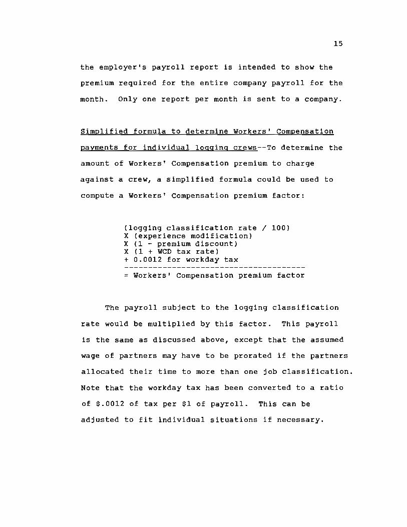
Simplified formula to determine Workers' Compensation
payments for individual loqqinq crews--To determine the
amount of Workers' Compensation premium to charge
against a crew, a simplified formula could be used to
compute a Workers' Compensation premium factor:
(logging classification rate / 100)X (experience modification)X (1 - premium discount)X (1 + WCD tax rate)+ 0.0012 for workday tax
= Workers' Compensation premium factor
The payroll subject to the logging classification
rate would be multiplied by this factor. This payroll
is the same as discussed above, except that the assumed
wage of partners may have to be prorated if the partners
allocated their time to more than one job classification.
Note that the workday tax has been converted to a ratio
of $.0012 of tax per $1 of payroll. This can be
adjusted to fit individual situations if necessary.

An example calculation demonstrates the use of this factor.
Given:logging classification rate = $27.50 I $100 of subject
payrollexperience modification = 0.95premiumWCD taxworkday
10% (.10)12% (.12)$.12/day or $.0012/$1 of
payroll
(27.50 I 100)X (0.95)X (1 - 0.10)X (1 + 0.12)+ 0.0012
dogging classification rate:experience modification:premium discount:WCD tax:workday tax
16
= 0.2645 :Workers' Compensation premium factor
Calculation of amount of Workers' Compensation premium:
($9,000 + $1,000) X 0.2645 = $2,645
Limitations of usinq the Workers' Compensation
simplified formula--There are several shortcomings to be
aware of when using the formula discussed above to
determine the amount of Workers' Compensation premium to
apply to a crew. Only the regular portion of overtime
pay is subject to Workers' Compensation premiums. If
the overtime portion of overtime pay is multiplied by
the Workers' Compensation factor, premium cost will be
overestimated. Also, the workday tax calculated will
discount =
rate =
tax =
subject payroll = $9,000(hourly plus salaried)
assumed wages subject = $1,000(prorated partners)
Calculation of factor:

17
not be exact since the tax rate is being converted from
a dollar per day figure to a ratio of workday tax paid
per dollar of payroll. However, this amount is usually
small and should not make a large difference in the
labor cost. Finally, the first $2,500 (1986 figure) of
annual premium is not subjected to a premium discount.
The formula to calculate the Workers' Compensation
factor does not take this into account.
Most companies tracking labor cost will not need
to consider these shortcomings when calculating a
Workers' Compensation factor. If this is the case, a
company should calculate a Workers' Compensation factor
using the simplified formula described above and use
this factor for the entire premium period.
SOCIAL SECURITY TAX--Social Security is a plan for old-
age pensions, survivors' benefits, and health or
disability insurance administered by the U.S. government
and maintained by federal funds of certain groups of
employers and their employees. Logging employees,
including partners and salaried employees, are subject
to Social Security tax. The social security rates are
set yearly by Congress and take effect on January 1.
For 1986, the tax rate is 15.30% of gross wages to an
upper limit of $42,000 per employee. If an employee
makes more than $42,000 in gross wages during the

18
calendar year, no Social Security tax would be paid on
the amount over $42,000. Social Security tax is split
50%-50% between the employer and employee. This means
that for 1986 the employer contributed 7.15% to the
Social Security tax while the employee contributed the
other 7.15%. The employer contribution to Social
Security tax is required to be paid within three banking
days after payday. Monetary incentive pay is subject to
Social Security tax. However, Social Security tax is
paid only if wages plus incentive pay remains below
$42,000. Social Security tax contributed 4.8% and 5.3%
to the total labor cost for Company A and Company B
respectively.
Availability of Social Security tax records--Although
Social Security tax payments are due by the employer
within three banking days of payday, a report is filed
quarterly to the Social Security agency. This is
Federal Form 941 and it shows the amount of total
company payroll, the amount of payroll subject to Social
Security tax, and the employer contribution to Social
Security tax. An employer could determine the exact
ratio of Social Security payment to total wages by
dividing total Social Security tax paid for the year by
total company wages paid for the same year. For logging
crews it would be easier to multiply the total crew

wages by the non-adjusted Social Security tax rate
(employer's contribution) to determine total cost of
Social Security. This method can be Justified since
very few logging personnel make over $42,000 in gross
wages during a year.
STATE UNEMPLOYMENT TAX--State unemployment taxes are
wholly an employer contributions The unemployment tax
rate (for the state of Oregon) is determined as follows
A "benefit ratio" for an employer is calculated by
dividing the benefits charged to an employer by the
taxable payroll. "Taxable payroll includes payroll for
a maximum of 12 calendar quarters preceeding July 1 of
the previous year. Taxable payroll for unemployment tax
purposes is set at an upper limit of gross wages per
employee. For example, for 1985 the taxable payroll was
set at an upper limit of $13,000 per employee. In 1986,
the taxable payroll limit was raised to $14,000 per
employee. "Benefit charges" are the benefits paid out
and charged to an employer's account. The benefit
charges used for the calculation of the benefit ratio
are for the same time period as the taxable payroll.
The unemployment tax rate is determined by the benefit
ratio--the higher the ratio, the higher the tax rate.
For 1986, Oregon's unemployment tax rates varied from a
low of 2.2% of subject wages (the first $14,000 of gross
19
20
wages per employee) to a high of 5.4% of subject wages.
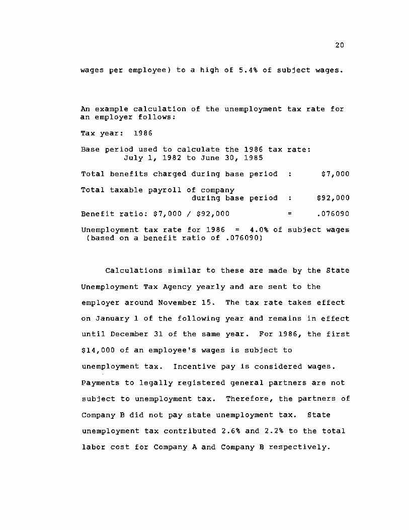
An example calculation of the unemployment tax rate foran employer follows:
Tax year: 1986
Base period used to calculate the 1986 tax rate:July 1, 1982 to June 30, 1985
Total benefits charged during base period
Total taxable payroll of companyduring base period
Benefit ratio: $7,000 / $92,000
$7,000
$92,000
.076090
Unemployment tax rate for 1986 = 4.0% of subject wages(based on a benefit ratio of .076090)
Calculations similar to these are made by the State
Unemployment Tax Agency yearly and are sent to the
employer around November 15. The tax rate takes effect
on January 1 of the following year and remains in effect
until December 31 of the same year. For 1986, the first
$14,000 of an employee's wages is subject to
unemployment tax. Incentive pay is considered wages.
Payments to legally registered general partners are not
subject to unemployment tax. Therefore, the partners of
Company B did not pay state unemployment tax. State
unemployment tax contributed 2.6% and 2.2% to the total
labor cost for Company A and Company B respectively.

21
Availability of state unemployment tax records--In
Oregon, state unemployment taxes are paid quarterly by
the employer. All subject wages, including advances,
are reportable when paid to the employee. For example,
if the wages were earned for the period March 15 to
March 30 but paid on April 5, the wages would be
recorded in the second quarter (April-June). State form
136, a quarterly reporting form, is completed by the
employer and sent to the Oregon Employment Division.
This report contains the following information: number
of covered workers for each month of the quarter; the
total wages paid to covered workers for the quarter; the
excess wages, or amount of wages paid during the quarter
in excess of the taxable wage base; and the taxable
wages, calculated by subtracting the excess wages from
the total wages. Also required on this report is a
listing of all employees that are being reported. This
listing includes Social Security number, name, number of
weeks worked during the quarter, and total wages paid
during the quarter.
Determininq the proper state unemployment tax rate to
charqe loqqinq crews--Since the upper limit of subject
wages is relatively low ($14,000 for 1986), it is safe
to assume that many members of the crew will reach this
limit while others may not. This means that the

22
unemployment tax rate for the company decreases as more
employees reach the upper payroll limits. To compensate
for this, a company can calculate a prorated
unemployment tax rate by dividing the total state
unemployment tax paid for all members of the crew by the
total wages paid to the same crew members for the same
time period (usually one year). The neccessary dollar
amounts can be obtained from the unemployment tax
records. This prorated tax rate must be calculated at
least once a year due to potential annual changes in the
upper limits of subject wages.
FEDERAL UNEMPLOYMENT TAX--Federal unemployment tax Is
used by the federal government to supplement
unemployment benefits to workers. The tax is wholly an
employer contribution. The tax rate is set by Congress
and remains in effect for the entire year. For 1986,
the federal unemployment tax rate was 0.8% of gross
wages to an upper subject wage limit of $7000. Monetary
incentive pay is considered wages. Payments to legally
registered partners are not subject to federal
unemployment tax. Federal unemployment tax contributed
0.5% and 0.4% to the total labor cost for Company A and
Company B respectively.

Availability of federal unemployment tax records--
Federal unemployment taxes are paid quarterly by the
employer. Federal Form 940 is used. The form shows
total wages paid, excess wages paid, and federal
unemployment tax due. There is no provision to list
individual employees on the federal unemployment tax
form as there is on the state form. Payment is due
within one month of the end of the quarter.
Determininq the proper federal unemployment tax rate to
charqe loqqinq crews--Since the upper limit of subject
wages is relatively low ($7,000 for 1986), it is safe to
assume that most crew members will reach this upper
limit while a few may not. This means that the federal
unemployment tax rate for a company will decrease as
more crew members reach the upper limit. The options to
solving this problem are the same as those for state
unemployment tax.
HEALTH INSURANCE--The portion of health insurance
premiums that are paid for by the employer must be
considered as part of the total employer labor cost.
Company A had a health insurance plan for the members of
the logging crews. Premiums were paid monthly, however
an employee had to be employed by the company for three
months before being covered by the insurance plan.
23

24
Records for the monthly premium and employees covered
were easily obtained from the insurance company.
Company B had a health and life insurance plan for the
three partners. Only one hourly employee was covered by
a company health insurance plan. Records for Company B
were also easy to obtain. Health insurance contributed
1.7% to the total labor cost for Company A. Health and
life insurance contributed 2.6% to the total labor cost
for Company B.
Determininq the proper health and/or life insurance rate
to charqe loqqinq crews--The proper amount to charge
logging crews for health insurance is complicated when
some employees are covered by the plan while others are
not. Company A tracked the insurance cost of each
individual employee by assigning a daily rate for
insurance and multiplying this rate by the number of
days an employee worked on a particular crew. This was
done manually and was very time consuming.
An easier way to track health and life insurance
cost is to determine the amount of insurance premiums
paid for each dollar of total wages. Cost of insurance
premiums for the logging labor force of a company for an
entire year would be determined from insurance records.
This amount would then be divided by the total wages for
the logging labor force for the same time period. It
25
may be necessary to determine a separate rate for
partners versus hourly employees as was the case for
Company B. In either case, monetary incentive pay would
not be subject to the rates developed for health and/or
life insurance.
DEVELOPING A LABOR BURDEN FACTOR--The discussion above
described the labor cost components as a percentage of
the total labor cost. There is another way of
expressing labor cost that is frequently used. This is
known as a labor loading, labor burden cost, or simply
labor burden. Labor burden can be described as the
amount of additional cost incurred above wages to
operate a crew. Labor burden is normally expressed as a
percent or ratio of wages.
Some contractors may wish to include salaried
employees along with the hourly wage employees when
determining labor burden cost. There would be no
errors in doing this as long as the same labor burden
factors applied to the salaried employees and hourly
employees. Partner draws, on the other hand, should be
handled with a separate labor burden factor since they
are not subject to unemployment tax and may not be
subject to Workers' Compensation charges. As a basic
example, assume that the following rates apply to a
logging contractor:

LABOR BURDEN FACTOR: HOURLY AND SALARIED EMPLOYEES
Workers' Compensation factor($25/$lOO of wages) or $0.2500 / $1 of wages
Social Security tax(7.15% rate) or $0.0715 / $1 of wages
State Unemployment tax(5.00% rate) or $0.0500 / $1 of wages
Federal Unemployment tax(0.80% rate) or $0.0080 / $1 of wages
Health and/or Life Insurance: $0.0250 / $1 of wages
26
TOTAL LABOR BURDEN FACTOR: $0.4045 / $1 of wages
(Note that this labor burden factor is expressed asa ratio of wages. It could also be expressed as40.45% of wages.)
LABOR BURDEN FACTOR: PARTNER DRAWS
Social Security tax(7.15% rate) or $0.0715 / $1 of draws
Health and/or Life Insurance: $0.1250 / $1 of draws
TOTAL LABOR BURDEN FACTOR: $0.1965 / $1 of draws
(This labor burden factor can also be expressed as19.65% of draws.)
In this simple example, the total hourly plus
salaried employee wages would be multiplied by one labor
burden factor and any partner draws (assigned to the
logging crew) would be multiplied by another labor
burden factor. The total wages, draws, and labor burden
cost would be added together to come up with a total
labor cost for the crew. An example helps illustrate
this:
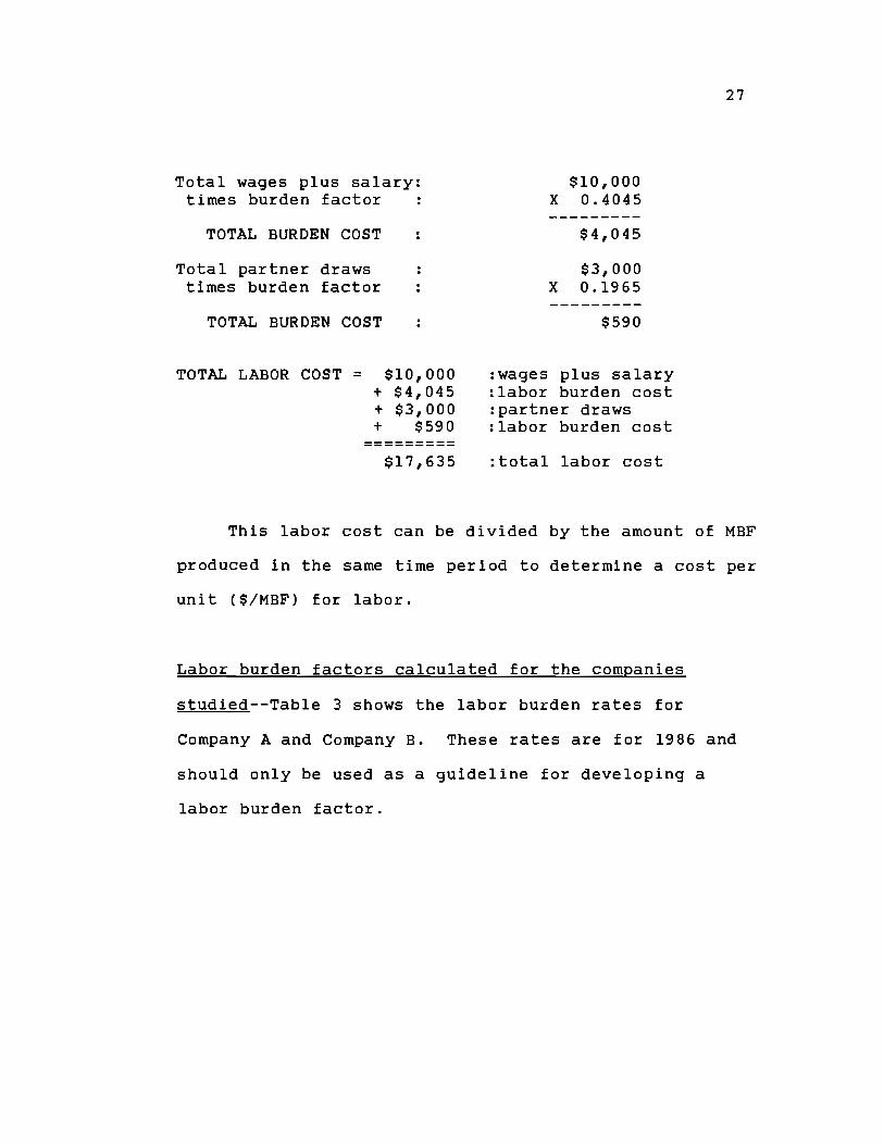
Total wages plus salary: $10,000times burden factor : X 0.4045
TOTAL BURDEN COST $4,045
Total partner draws $3,000times burden factor X 0.1965
TOTAL BURDEN COST $590
TOTAL LABOR COST = $10,000 :wages plus salary+ $4,045 :labor burden cost+ $3,000 :partner draws+ $590 :labor burden cost
$17,635 :total labor cost
This labor cost can be divided by the amount of MBF
produced in the same time period to determine a cost per
unit ($/MBF) for labor.
Labor burden factors calculated for the companies
studied--Table 3 shows the labor burden rates for
Company A and Company B. These rates are for 1986 and
should only be used as a guideline for developing a
labor burden factor.
27

Table 3. LABOR BURDEN FACTOR FOR COMPANY A AND COMPANY BEXPRESSED AS A PERCENT OF WAGES.
COMPANY A COMPANY BW/O PARTNERS W/PARTNERS
WORKERS' COMPENSATIONSOCIAL SECURITYSTATE UNEMPLOYMENTFEDERAL UNEMPLOYMENTHEALTH INSURANCE
21 . 51%
7. 15%3.90%0.80%2.50%
35.94%
29.10%7 .15%4. 20%0.80%0.28%
28
21. 00%7 . 15%
3 . 03%
0. 58%3.53%
41.53% 35.29%
These rates do not use a prorated state unemployment norfederal unemployment tax rate. Actual labor burden maybe lower if a prorated tax rate were used.
Strenqths of usinq the labor burden factor--The labor
burden factor described above is relatively simple to
calculate and use. Computers are not required for its
use. The factors needed to derive the labor burden
factor are available from existing records. Health
and/or life insurance is the most difficult factor to
derive since some calculation is required to determine
the proper amount of premium and total wages to use.
Total wages can be multiplied by the labor burden factor
(care must be taken if partner draws are being
considered) to come up with a total labor burden cost.
Labor burden cost and all wages, draws, and salary are
added together to give an estimate of the total labor
cost.

29
Weaknesses of usinq the labor burden factor--There are
several weaknesses to using the labor burden factor as
described above, especially if the labor burden cost is
to be charged against a crew on monetary incentives.
Multiplying total wages by a labor burden factor
subjects any overtime portion of overtime pay to
Workers' Compensation. Since the overtime portion of
overtime pay should not be charged for Workers'
Compensation premiums, this can overestimate a crew's
labor cost. Second, some inaccuracies in the
calculation of unemployment tax and possibly Social
Security tax will result since the prorated tax rates
used in calculating the labor burden may not be the
actual rates paid.
Recommendations in usinq the labor burden factor--If a
logging contractor wished to use the labor burden factor
simply to track labor cost for planning purposes, the
use of an "unadjusted" labor burden factor may be
appropriate, especially if a minor amount of overtime is
worked during the season. However, if overtime is
frequently worked, only the wages subject to Workers'
Compensation (straight-time wages and the straight-time
portion of overtime wages) should be multiplied by the
Workers' Compensation factor. The total wages would be

30
multiplied by the remaining labor burden factor to
calculate the remaining labor cost.
If the labor cost is being charged against a crew
on a monetary incentive program then it may be desirable
to calculate the labor cost as accurately as possible.
This means charging the proper rate for all components
of the labor cost.
Regardless of which method to calculate the labor
burden is chosen, the limitations must be fully
understood. This becomes more important when crews are
on monetary incentives.
Some examples will help to illustrate the
differences in using the labor burden factor. Example 1
shows the effects of charging an unadjusted labor burden
factor against total wages. Example 2 adjusts the labor
burden factor for state and federal unemployment tax and
charges Workers' Compensation against only the straight-
time portion of wages. Example 3 shows a precise method
for tracking the actual labor cost for a logging crew.

TOTAL LABOR COST = Total wages plus salary+ Labor burden cost
(hourly plus salaried)+ Total partner drawsLabor burden cost (partners)
TOTAL LABOR COST = $29,500($29,500 X 0.4045)
+ $5,000+ ($5,000 X 0.1965)
31
Example 1. This example shows the use of an unadjustedlabor burden factor and multiplies totalwages by the Workers' Compensation rate.Also, state and federal unemployment ratesare not prorated.
HOURLY EMPLOYEES
Wagesstraight time portion $27,500overtime portion $2,000Total wages $29,500
Labor BurdenWorkers' Compensation $0.2500 / $1 of wagesSocial Security tax $00715 / $1 of wagesstate unemployment tax $0.0500 / $1 of wagesfederal unemployment tax $0.0080 / $1 of wageshealth and/or life insurance $0.0250 / $1 of wages
BURDEN FACTOR $0.4045 / $1 of wages
Labor BurdenSocial Security tax $0.0715 / $1 of drawshealth and/or life insurance $0.1250 / $1 of draws
BURDEN FACTOR $0.1965 / $1 of draws
= $29,500= $11,933= $5,000= $983
$47, 416
PARTNER DRAWS
Drawsstraight time portion $5,000overtime portion $0

Example 2. This example shows the use of the labor burdenfactor, but multiplies only the straight-timeportion of wages by the Workers' Compensationfactor. Also, assumed prorated state andfederal unemployment tax rates are used.
HOURLY EMPLOYEES
TOTAL LABOR COST = $29,500+ ($27,500 X 0.2500)+ ($29,500 X 0.1343)+ $5,000+ ($5,000 X 0.1965)
32
TOTAL LABOR COST = Total wages plus salary+ Workers' Compensation burden+ Remaining labor burden
(hourly plus salary)+ Partner draws+ Labor burden (partner)
= $29,500= $6,875= $3,962= $5,000= $983
$46,320
The difference in labor cost between example 1 andexample 2 is $1,096.
Wagesstraight time portion $27,500overtime portion $2,000
Total wages $29,500
Labor BurdenWorkers' Compensation $0.2500 / $1 of wagesSocial Security tax $0.0715 / $1 of wagesstate unemployment tax $0.0350 / $1 of wagesfederal unemployment tax $0.0028 / $1 of wageshealth and/or life insurance $0.0250 / $1 of wages
BURDEN FACTOR FOR WORKERS' COMP. $0.2500 / $1 of wagesBURDEN FACTOR FOR REMAINING ITEMS $0.1343 / $1 of wages
PARTNER DRAWS
Drawsstraight time portion $5,000overtime portion $0
Labor BurdenSocial Security tax $0.0715 / $1 of drawshealth and/or life insurance $0.1250 / $1 of draws
TOTAL BURDEN FACTOR $0.1965 / $1 of draws
33
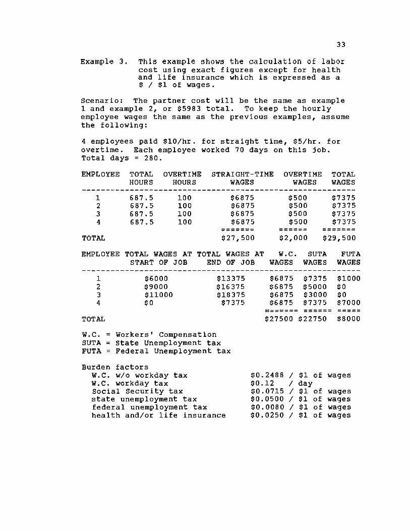
Example 3. ThIs example shows the calculation of laborcost using exact figures except for healthand life insurance which is expressed as a$ I $1 of wages.
Scenario: The partner cost will be the same as example1 and example 2, or $5983 total. To keep the hourlyemployee wages the same as the previous examples, assumethe following:
4 employees paid $10/hr. for straight time, $5/hr. forovertime. Each employee worked 70 days on this job.Total days = 280.
EMPLOYEE TOTAL OVERTIME STRAIGHT-TIME OVERTIME TOTALHOURS HOURS WAGES WAGES WAGES
$0.2488 / $1 of wages$0.12 / day$0.0715 /$0.0500 /$0.0080 /$0.0250 /
$1 of wages$1 of wages$1 of wages$1 of wages
$7375 $1000$5000 $0$3000 $0$7375 $7000
$22750 $8000
1 687.5 100 $6875 $500 $73752 687.5 100 $6875 $500 $73753 687.5 100 $6875 $500 $73754 687.5 100 $6875 $500 $7375
TOTAL $27,500 $2,000 $29,500
EMPLOYEE TOTAL WAGES AT TOTAL WAGES AT W.C. SUTA FUTASTART OF JOB END OF JOB WAGES WAGES WAGES
1 $6000 $133752 $9000 $163753 $11000 $183754 $0 $7375
TOTAL
W.C. = Workers' CompensationSUTA = State Unemployment taxFUTA = Federal Unemployment tax
Burden factorsW.C. w/o workday taxW.C. workday taxSocial Security taxstate unemployment taxfederal unemployment taxhealth and/or life insurance
$6875$6875$6875$6875
$27500
EXAMPLE 3 CONTINUED
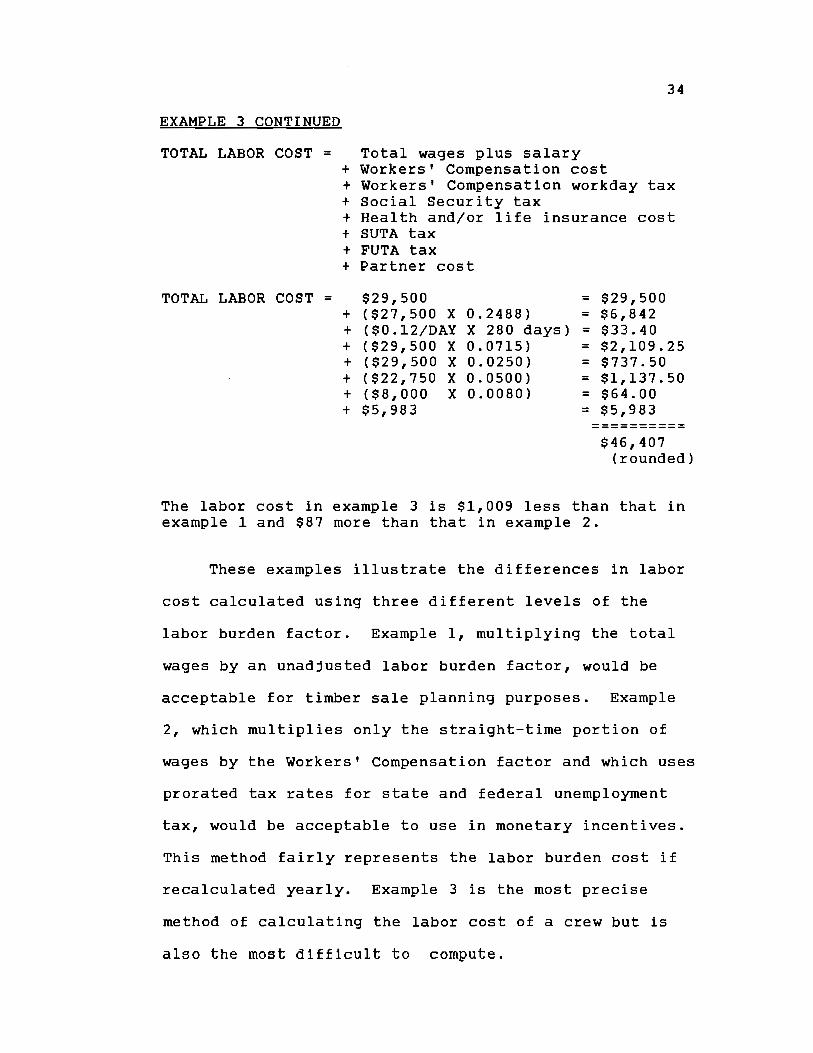
TOTAL LABOR COST = Total wages plus salary+ Workers Compensation cost+ Workers' Compensation workday tax+ Social Security tax+ Health and/or life insurance cost+ SUTA tax+ FUTA tax+ Partner cost
TOTAL LABOR COST = $29,500 = $29,500+ ($27,500 X 0.2488) = $6,842+ ($0.12/DAY X 280 days) = $33.40+ ($29,500 X 0.0715) = $2,109.25+ ($29,500 X 0.0250) = $737.50+ ($22,750 X 0.0500) = $1,137.50+ ($8,000 X 0.0080) = $64.00+ $5,983 = $5,983
34
$46,407(rounded)
The labor cost in example 3 is $1,009 less than that inexample 1 and $87 more than that in example 2.
These examples illustrate the differences in labor
cost calculated using three different levels of the
labor burden factor. Example 1, multiplying the total
wages by an unadjusted labor burden factor, would be
acceptable for timber sale planning purposes. Example
2, which multiplies only the straight-time portion of
wages by the Workers Compensation factor and which uses
prorated tax rates for state and federal unemployment
tax, would be acceptable to use in monetary incentives.
This method fairly represents the labor burden cost if
recalculated yearly. Example 3 is the most precise
method of calculating the labor cost of a crew but is
also the most difficult to compute.
THE EQUIPMENT COST COMPONENT
Standard equipment cost calculations include
allowances for both ownership and operating costs. The
ownership portion of equipment cost includes purchase
price (new or used), salvage or residual value,
depreciation, property tax, insurance premiums, lost
opportunity cost (interest foregone), and any fees
required for license and storage of the equipment.
Operating costs include fuel, lube and oil, repair and
maintenance, track or tire replacement, and wire rope
replacement. These cost components are used in standard
engineering formulas such as average annual cost to
determine the cost which must be recovered for a piece
of equipment to break even. This is also the cost which
would be charged against a crew on monetary incentives
for use of the particular piece of equipment.
This report identifies the equipment cost
components that a logging contractor needs to track,
what cost records are available, and identifies areas
where better records must be kept. There is also some
discussion on the use of standard equipment cost
formulas such as the Average Annual Investment (AAI) and
marginal cost (next year's actual cost). A thorough
discussion and derivation of the AAI method of equipment
cost calculation can be found in Appendix C. Sample
35
calculations of equipment cost using both the average
annual cost method and the marginal cost method can also
be found in Appendix C.
OWNERSHIP COSTS--Ownership costs consist of
depreciation, property tax, insurance cost, lost
opportunity cost, and storage and license fees.
Ownership costs are also known as fixed costs and occur
whether the piece of equipment is being operated or
sitting idle. Ownership costs are expressed on an
annual cost basis or more commonly on a dollar per
yearly scheduled machine hour basis (scheduled machine
hours per year can be described as the number of shifts
per year a machine is expected to work multiplied by the
average hours per shift). Each component is described
and the availability and use of existing records is
discussed for each component.
Depreciation--Depreciation is the decrease in worth of
an asset over time. Depreciation of logging equipment
is brought about by the everyday wear and tear of
operation gradually lessening the capability of the
piece of equipment to perform its intended function. To
a lesser extent, depreciation of logging equipment can
be brought about by technological advances which makes a
current piece of equipment obsolete.
$110,000 (depreciable amount)
If the estimated useful life is 8 years and thescheduled machine hours (SMH) per year are estimated tobe 1600 (200 days/year X 8 hours/shift), then thedepreciation cost becomes:
$110,000 / 8 years = $13,750 / year[$13,750 / year] / [1600 SHH / year] = $8.59 / SMH
The method used above to calculate depreciation is
the Straight-Line method and is normally used in
equipment cost calculations due to its compatability
with the AM formula and its ease of use.
Availability of records needed to comDute depreciation
cost--In order for a logging contractor to estimate
37
Depreciation is recovered by subtracting the
salvage value from the purchase price and dividing the
result by the estimated useful life in years of the
equipment. Normally, purchase price is reduced by the
cost of track, tire, or wire rope replacement. If the
scheduled machine hours per year are known an hourly
cost is calculated. An example for a crawler tractor
would be as follows:
$150,000 (purchase price plus tax and freight)- 10,000 (track replacement cost)
=
$140,000- 30,000 (salvage value)

38
depreciation cost, five values must be known: purchase
price, track, tire, or line replacement costs, salvage
value, estimated useful life in years for the piece of
equipment, and scheduled machine hours of use per year
for the piece of equipment. It is relatively easy to
get purchase prices and track, tire, and line
replacement cost from an equipment dealer, but the
remaining figures are not always so easy to obtain. For
example, salvage value of a piece of equipment can range
anywhere from 0% to 30% of original purchase price.
Useful life and scheduled hours per year are
estimates and often change. If a company kept records
on similar pieces of equipment, then salvage value and
life can be more accurately predicted. Neither Company
A nor Company B kept records of this sort. The
Caterpillar Performance Handbook is a good reference for
estimating total ownership hours for a piece of
equipment based on application and operating conditions.
See Appendix D for an adaptation of this guide.
Weaknesses of usinq depreciation cost in monetary
incentives--Although depreciation is a major component
of equipment cost and is essential for cost control and
planning, there are several weaknesses when applying it
to monetary incentives. First, the estimates used for
salvage value, years of life, and scheduled hours of use

39
can severely overcharge or undercharge a crew. As a
simple example, assume that the depreciable amount
calculated above ($110,000) is correct, the actual hours
worked during the year is close to 1600, but the life of
the machine turns out to be nine years instead of the
estimated eight years. The actual yearly cost of
depreciation would be $12,222 for nine years as compared
to $13,750 for eight years. Actual hourly cost would be
$7.64 for nine years compared to $8.59 for eight years.
This means that the crew could be overcharged $0.95 in
depreciation charges alone for each hour the machine is
used. On the other hand, if the life of the machine
turns out to be only seven years, then the contractor
would be undercharging the crew $1.23 (an hourly cost of
$9.82 for a seven-year life versus an hourly cost of
$8.59 for an eight-year life).
Opportunity Cost--Opportunity cost is the amount of
money a logging contractor foregoes by investing in a
particular piece of equipment. If capital was borrowed
to purchase the piece of equipment, the interest rate is
established by the lender. The yearly opportunity cost
becomes the amount of interest paid per year. If cash
was used to purchase the equipment, the opportunity cost
is the amount of money, or return, the contractor would
like to receive if his money was invested elsewhere.
40
Typical rates of return ranqe from 1O to 15. In the
AAI method of equipment costing, the yearly rate of
return (expressed as a decimal), is multiplied by the
AAI to determine the total amount of revenue needed to
recover the opportunity cost. This cost is converted to
a dollar per hour basis by dividing the total yearly
opportunity cost by the scheduled machine hours for the
year.
Availability of records for calculatinq an opportunity
cost--There is no standard formula available for
calculating a rate of return for an opportunity cost.
If the equipment is financed, the rate of return used is
the interest rate set by the lending institution. If
the equipment is financed with company funds, a good
starting point for a rate of return is the going
interest rate given on loans for equipment purchase. A
company could use this rate or raise or lower it as they
feel necessary. If the company has a rate of return
they are willing to accept for invested income, then
this rate should be used in the calculation of
opportunity cost.
Opportunity cost is a difficult concept for many
contractors to understand and many do not have an
established rate of return for company investments.
Neither Company A nor Company B had a rate of return for

41
invested income. The opportunity cost is a major
component of the equipment cost and the selection of a
realistic rate of return greatly influences the dollar
per hour ownership cost for a piece of equipment. See
Appendix C for an example calculation of the opportunity
cost.
Property Tax--Property tax is charged against the market
value of a piece of equipment assessed at the start of
the year. The rates vary depending on where the
equipment is located as of January 1 of the year.
Company A, for instance, had equipment located in
several counties and school districts on the first of
the year. As a result, Company A had approximately five
different property tax rates assessed for varying
amounts of equipment market values. To simplify this
problem, a weighted average property tax rate should be
calculated and applied against each piece of equipment.
Property tax is not assessed against licensed and
registered pickup trucks or crew vehicles.
Availability of property tax records--Property tax
records are readily available and relatively easy to
use. An individual billing is sent to the owner of the
property for each tax base area. The bill includes the
tax rate expressed in dollars per one thousand dollars

42
of market value and the total market value of the
equipment at the tax base location. Individual pieces
of equipment are not identified. The property tax for
an individual piece of equipment can be determined by
expressing the weighted average property tax rate as a
ratio of market value and multiplying the AAI by this
ratio. For example, if the property tax rate is $13.50
I $1000 of market value, the ratio of property tax to
market value is $0.0135 I $1 of market value. Since the
AAI represents the average annual investment or average
market value, an estimate of the hourly charge for
property tax for this example is:
(AAI X 0.0135) / scheduled machine hours = $/hr. charge
Since the property tax rate is based on the true
cash market value of a piece of property, the method
shown above is only valid when an average annual tax
payment is desired. It will not be the actual yearly
property tax payment for a piece of equipment. The true
annual tax payment will be higher or lower depending on
the age and market value of the piece of equipment being
costed. However, for planning purposes or monetary
incentives, an average annual payment may be used.
Insurance--Most logging contractors will carry insurance
43
on their logging equipment and vehicles to cover the
cost of any loss due to fire, theft, or other damage.
This cost must also be recovered when calculating the
hourly rate to own a piece of equipment. For both
Company A and Company B, insurance rates for logging
equipment were determined on a dollar per thousand
dollar of market value much the same as property tax.
The market value the insurance company used was the same
value used for property tax assessment. This makes the
calculation of insurance charges very simple.
Availability of insurance records--The rates charged for
insurance on a piece of equipment are readily available
from the insurance policy or by contacting the insurance
agent. Both Company A and Company B had a blanket
policy with insurance rates in the area of $8.00 I $1000
of market value regardless of the age of the equipment.
The method used to calculate the yearly insurance charge
for logging equipment is the same method used to
calculte the property tax charge. Vehicles such as
pickups used for crew travel are not charged the same
rate as other logging equipment. Typically, these
vehicles are charged a monthly policy premium. The
total yearly insurance payment is easily calculated from
these monthly payments.
44
Storaqe Fees--If there Is a charge for storage of a
piece of logging equipment, this charge must be
reflected in the dollar per hour rate calculated for the
ownership cost. Neither Company A nor Company B had any
fees charged for storage of equipment. Both companies
either kept the equipment on job sites during the year
or stored it at their own shop location. If storage is
being charged, it can be treated as a percent of AM
much like property tax or insurance, or the actual rate
can be determined by dividing the annual storage charge
by the scheduled machine hours for the year.
License Fees--Logging equipment including fire trucks is
not subject to licensing fees. Trucks used for highway
travel do have a license fee. The yearly license fee
must be divided by the yearly scheduled machine hours to
determine the dollar per hour charge. Another option is
to treat the license fees as a percent of AM.
Handlinq inflation in ownership costs--Since the costs
calculated by the AM method are for a base year, the
effect of inflation should be taken into account.
Multiplying the current ownership cost by the annual
rate of inflation adjusts for the effects of inflation.
For example, if the calculated ownership cost is
$20.00/hour in the base year (1987), and the inflation
45
rate for 1988 is estimated to be 5%, then the ownership
cost for 1988 would be recalculated to be: $20.00/hour X
1.05 = $21.00/hour.
This method assumes that all components of the
ownership cost are inflating at the same rate. An
example of inflating ownership costs can be found in
Appendix C. The bottom line when dealing with inflation
is to realize that the costs calculated in the base year
will not be high enough to cover the same costs in
future years due to the effects of inflation.
When to use the AAI method or the marqinal cost method
for calculatinq ownership costs--As discussed in
Appendix C, the AAI method calculates the average
capital invested in a piece of equipment during its
estimated useful life. If a piece of equipment is used
beyond its estimated useful life, it is technically
incorrect to use the AAI method to estimate ownership
costs. This is because the estimated life of the
equipment (from a calculation standpoint) is now zero
years and the average capital invested in the piece of
equipment is now the current market value. This current
market value may not be the same as the salvage value
used in the AAI calculation.
It is neccessary to switch to a marginal cost (next
year's actual cost) if a piece of equipment is used
46
beyond its useful life. The opportunity cost, property
tax, insurance costs, and, if applicable, license fees
and storage, should be expressed as a ratio of current
market value. Depreciation charges are no longer
calculated since these charges have been recovered.
Ownership costs using the marginal cost method should be
calculated yearly due to flucuations in market value for
a piece of equipment. These ownership costs will be
much less than those estimated using the AAI method but
more accurately portray the true ownership costs.
Inflation will be taken into account if ownership costs
are calculated yearly using the marginal cost method. A
sample calculation using the marginal cost method for
ownership cost is found in Appendix C.
OPERATING COSTS--Operating costs include fuel and lube
costs, tire, track, and wire rope replacement costs, and
repair and maintenance costs. Operating costs are also
known as variable costs and are the result of operating
a piece of equipment. Operating costs are converted to
a cost per scheduled machine hour so that they can be
added to ownership costs to arrive at a total cost per
scheduled machine hour. This report describes each
component of the operating cost. In addition, the
records available to a logging contractor to track these
costs and the ease of using these records is evaluated.

47
Where available, standard formulas, guidelines, and
references are given to allow a contractor to estimate
operating costs when records are lacking.
Fuel and Lube-- Company A did not measure fuel or lube
consumption but rather gave an estimate of the amount of
fuel used per machine hour (a machine hour is 60 minutes
of machine work) for each piece of equipment studied.
Company B purchased a fuel meter at the start of the
study and tracked fuel consumption and machine hours of
use for each piece of equipment studied. Use of
lubricants was not tracked.
It's important to convert fuel and lubricant
consumption based on machine hours to fuel and lubricant
consumption based on scheduled machine hours. For
example, if a piece of equipment uses 4.0 gallons of
fuel for each machine hour it works but only works 6
machine hours out of a scheduled eight hour shift, then
fuel consumption per scheduled machine hour becomes:
4.0 gallons 6 machine hoursX =3.0 gallons/SMH
machine hour 8 scheduled machine hours
This 3.0 gallons per hour figure can be multiplied
by the dollar per gallon cost for fuel to determine the
cost per hour for fuel consumption:
3.0 gallon / SMH X $0.80 / gallon = $2.40 I gallon
48
Availability of fuel and lubricant records--Fuel and
lubricant records are available to logging contractors.
In many instances, fuel and lube is delivered to the job
site. The receipt for the fuel and lube usually shows
the amount and type delivered and the unit cost for
each. In order for a contractor to calculate an
accurate average fuel and lube cost it is necessary to
analyze fuel and lube records for a fairly long period
of time, perhaps for a year or longer. A weighted
average cost for a gallon of diesel and gasoline can be
calculated from the fuel records. The total cost for
lubricants for a period of time can be divided by the
total cost of diesel and gasoline for the same time
period to determine a prorated cost of lubricants for
each dollar of fuel.
Another option a logging contractor has is to
use the current cost of fuel and lubricants and update
these costs when major price changes occur. This option
has the advantage of being easy to use but does require
good estimates of both fuel and lubricant consumption.
Once the fuel consumption per scheduled machine
hour has been determined for a piece of equipment, the
dollar per hour fuel cost can be calculated by
multiplying the fuel consumption by the cost..
Lubrication cost can be estimated by multiplying fuel
cost by the prorated lube cost or by using actual lube
consumption and cost figures. For example, if diesel
cost was determined to be $0.80 / gallon and lube was
calculated to be $0.16 / $1 of fuel (prorated lube
cost), then.a realistic cost for fuel and lube
consumption would be:
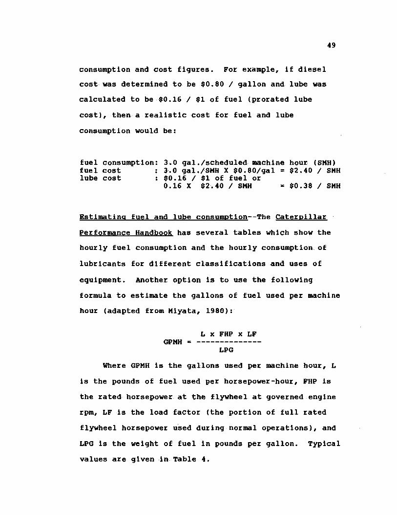
fuel consumption: 3.0 gal./scheduled machine hour (SMH)fuel cost : 3.0 gal./SMH X $0.80/gal = $2.40 / SMHlube cost : $0.16 / $1 of fuel or
0.16 X $2.40 / SMH = $0.38 / SMH
Estimatinq fuel and lube consumption--The Caterpillar
Performance Handbook has several tables which show the
hourly fuel consumption and the hourly consumption of
lubricants for different classifications and uses of
equipment. Another option Is to use the following
formula to estimate the gallons of fuel used per machine
hour (adapted from Miyata, 1980):
L x FHP x LFGPMH =
LPG
Where GPMH Is the gallons used per machine hour, L
is the pounds of fuel used per horsepower-hour, FHP is
the rated horsepower at the flywheel at governed engine
rpm, LF is the load factor (the portion of full rated
flywheel horsepower used during normal operatIons), and
LPG is the weight of fuel In pounds per gallon. Typical
values are given In Table 4.
49

Table 4. WEIGHTS, FUEL CONSUMPTION RATES, AND LOADFACTORS FOR DIESEL AND GASOLINE ENGINES.
(Adapted from Sessions and Miyata)
Engine Weight Fuel Consumption Load Factortype (LPG) (L) (LF)
lb / gallon lb / hp-hr Low Med High
Lubricant consumption in gallons (GPMH) per machinehour can also be estimated by the following formulas(adapted from Sessions):
These formulas include normal oil changes and no
leaks. They should be increased 25 percent when
operating in heavy dust, deep mud, or water. In
machines with complex and high pressure hydraulic
systems, such as forwarders, processors, and harvesters,
the consumption of hydraulic fluids can be much greater.
Another rule of thumb is that lubricants and grease cost
five to fifteen percent the cost of fuel.
These estimates of fuel and lubricant consumption
are calculated for a machine hour and must be converted
to gallons per scheduled machine hour as discussed above.
The cost per gallon for fuel or lubricants can then be
multiplied by the gallons consumed per scheduled machine
50
GPMH = 0.0002 x FHP (crankcase oil)GPMH = 0.00007 x FHP (transmission oil)GPMH = 0.00005 x FHP (final drives)GPMH = 0.00002 x FHP (hydraulic controls)
Ga so line 6.0 0.46 0.40 0.55 0.70
Diesel 7.1 0.42 0.40 0.55 0.70

51
hour to obtain a dollar per scheduled machine hour cost.
Tire, Track, or Wire Rope Replacement--Since tires,
tracks, and wire rope usually do not have the same life
as the piece of equipment, these items should be costed
out separately. At the time of purchase, the cost of
tire, track, or wire rope replacement should be
determined. Labor should be included in this cost. An
estimate of tire, track, or wire rope life needs to be
made so that a dollar per hour cost can be determined.
Availability of records to determine tire, track, or
wire rope replacement--Neither Company A nor Company B
kept records to determine the life or cost of tire,
track, or wire rope replacement. Replacement costs used
in standard equipment cost formulas often assume new
parts are used to replace the ones worn out. However,
new parts are not always used to replace old ones. It
is not uncommon to purchase used tracks or tires or to
salvage these items from other machines. It is also not
uncommon to do a partial replacement of tires or tracks.
Estimates of tire, track, and wire rope life vary
tremendously depending on operator, terrain, harvest
conditions, and even weather.
A good record keeping system that tracks yearly
replacement costs for individual pieces of equipment is
desired for determining accurate costs. If records are

52
kept, a cummulative hourly cost can be derived by
determining the total replacement cost and dividing this
by the total scheduled machine hours during the same
time period. For example, if for a three year period
the total cost of track replacement was $10,000 and the
total scheduled machine hours was 4800 hours, then the
total cummulative hourly cost for track replacement
becomes $10,000 / 4800 hours = $2.08 / hour.
Estimatinq tire, track, and wire rope life--There are
few sources available that give estimates of tire,
track, or wire rope life. Tire and track life are often
expressed in hours while wire rope life is often
expressed in total production achieved before
replacement is required. Equipment dealers,
manufacturers, and logging supply companies may be able
to give an estimate of life. The Caterpillar
Performance Handbook gives an estimate of tire life
based on application zones. Zone A is where almost all
tires actually wear through to the tread due to abrasion
only. Zone B includes tires wearing out but others
failing prematurely due to rock cuts, rips, and non-
repairable punctures. Zone C has few if any tires ever
wearing through the tread before having to be discarded,
usually from rock cuts. Based on these application
zones, the following tire life can be estimated.

TABLE 5. ESTIMATED TIRE LIFE BASED ON APPLICATIONZONE. (Adapted from the CaterpillarPerformance Handbook)
Note: The values found in this table are estimates ofmachine hours and must be converted to scheduled machinehours by the same method described in the section onfuel and lube consumption.
This table is based on the following assumptions:
New tires are run to destruction (this is notnecessarily recommended).
Standard machine tires are used. Optional tires canbe outside of these ranges.
Sudden failures due to exceeding tire rated loadingis not considered, nor are premature failures due topunctures.
There is no known reference for estimating the life
of tracks. Track life depends on operating conditions,
terrain, and operator.
The U.S. Forest Service has developed a wire rope
life guide (Table 6) for cable logging systems in the
Pacific Northwest (McGonagill). This guide assumes the
wire rope is properly maintained and used in accordance
with manufacturer's recommendations.
53
Equipment Tire Life, HoursZone A Zone B Zone C
Skidders 4000-6000 200 0-4 0 0 0 1000-2000Wheel loaders 30 00-6000 100 0-30 00 500-1000Off-highway trucks 400 0-6 0 0 0 2000-40 00 1000-2000

TABLE 6. ESTIMATED WIRE ROPE LIFE BASED ON
54
Note: This table shows wire rope life based on totalproduction. For an example of converting wire rope lifeto total hours from total production, see Appendix E.
LoggingSystem
StandingSkyline
PRODUCTION. (McGonagill)
Line Line Size Line LifeUse (Inches) (MMBF)
Skyline 1 3/4 20 to 2511/2 15to2513/8 8to15
Mainline 1 lOtol5
LineClassification
6 x 216 x 216 x 216 x 26
Haulback 3/4 8 to 12 6 x 267/8 8 to 12 6 x 26
Live Skyline 1 1/2 10 to 20 6 x 21Skyline 1 3/8 8 to 15 6 x 21
1 6 to 10 6 x 26Mainline 1 10 to 15 6 x 26
3/4 8 to 12 6 x 265/8 8 6 x 26
Haulback 7/8 8 to 12 6 x 263/4 8 to 12 6 x 261/2 6 to 10 6 x 26
Slackpulling 7/16 5 to 8 6 x 26
Running Mainline 1 8 to 12 6 x 26Skyline Haulback 3/4 4 to 8 6 x 26
High Lead Mainline 1 3/8 8 to 15 6 x 261 1/8 6 to 12 6 x 26
Haulback 7/8 6 to 12 6 x 26
Strawline 3/8 to 5 to 8 6 x 197/16
Carriage Skidding 1/2 .5 6 x 267/8 3 to 5 6 x 26
Guylines 4 years 6 x 25
Skyline chokers 1/2 to .2 to .3 6 x 253/4

55
Weaknesses of usinq tire, track, or wire rope
replacement costs in a monetary incentive proqram--
Unless records have been kept on similar pieces of
equipment in similar operating conditions, the cost of
tire, track, or wire rope replacement is an estimate
that can severely overcharge or undercharge a crew on
monetary incentives. As a simple example, suppose an
estimate of tire replacement (at time of replacement)
for a skidder was $1200 per tire plus $300 in labor.
The estimated life due to the rough terrain was 1200
hours. Total cost for tire replacement would be
estimated at $5100 or $5100 / 1200 hours = $4.25 / hour.
If the tires actually lasted 1600 hours, this would
reduce the replacement cost to $3.19 / hour, or $1.06 /
hour less than originally estimated.
Repair and Maintenance--Repair and maintenance costs
include everything from routine maintenance items to
major overhauls of engines, transmissions, clutch,
brakes, or other major components. Routine lube and oil
changes are often covered under the lube and oil costs.
Normally, parts and labor are included in repair and
maintenance costs while shop and repair vehicles are
included in administrative overhead.
Records available for repair and maintenance cost--
Neither Company A nor Company B kept repair and
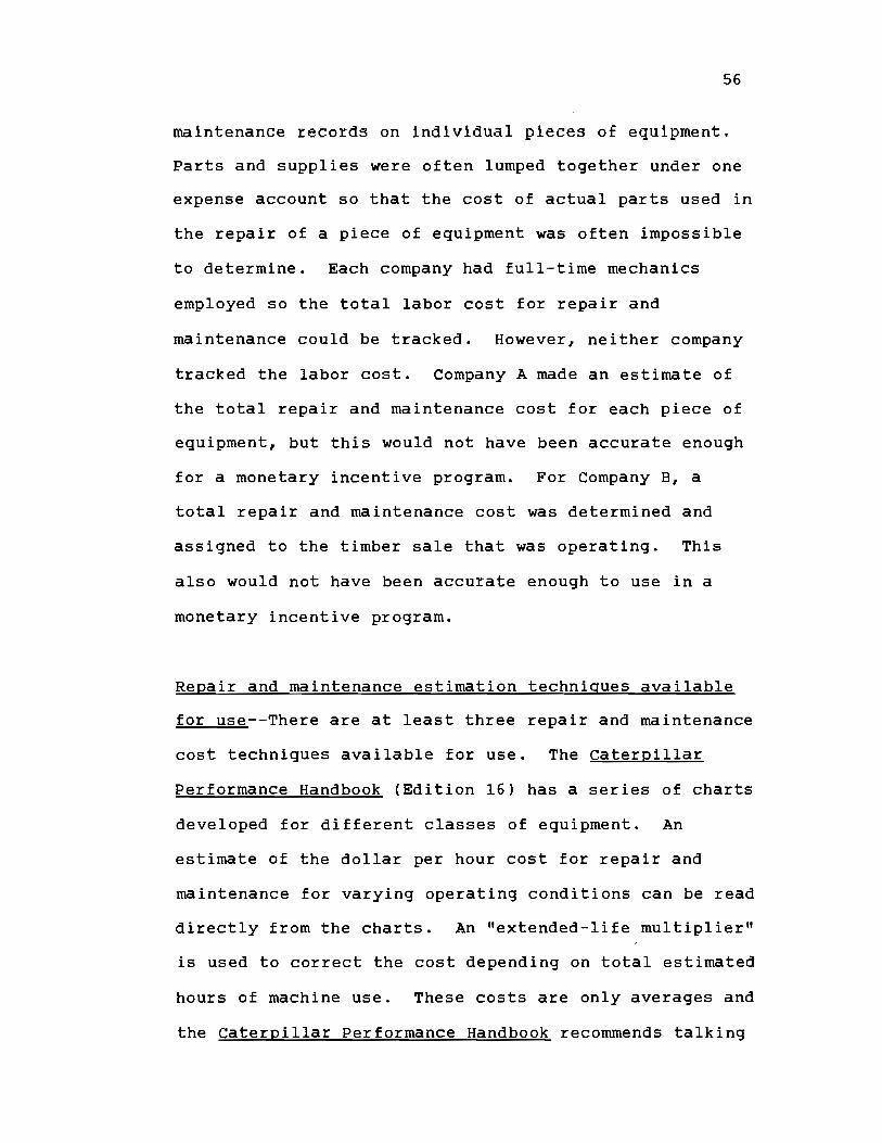
56
maintenance records on individual pieces of equipment.
Parts and supplies were often lumped together under one
expense account so that the cost of actual parts used in
the repair of a piece of equipment was often impossible
to determine. Each company had full-time mechanics
employed so the total labor cost for repair and
maintenance could be tracked. However, neither company
tracked the labor cost. Company A made an estimate of
the total repair and maintenance cost for each piece of
equipment, but this would not have been accurate enough
for a monetary incentive program. For Company B, a
total repair and maintenance cost was determined and
assigned to the timber sale that was operating. This
also would not have been accurate enough to use in a
monetary incentive program.
Repair and maintenance estimation techniques available
for use--There are at least three repair and maintenance
cost techniques available for use. The Caterpillar
Performance Handbook (Edition 16) has a series of charts
developed for different classes of equipment. An
estimate of the dollar per hour cost for repair and
maintenance for varying operating conditions can be read
directly from the charts. An "extended-life multiplier"
is used to correct the cost depending on total estimated
hours of machine use. These costs are only averages and
the Caterpillar Performance Handbook recommends talking

57
to a Caterpillar dealer for more accurate cost figures.
These costs also do not include any increase for
inflation and must be updated yearly. Also, any repair
and maintenance required for the undercarriage is
excluded from these charts and must be calculated
separately.
A second method which is. coonly used is to
estimate repair and maintenance cost as a percentage o
depreciation. Ranges typically given are shown in
Table 7 (adapted from Sessions, McGonagill, Miyata).
TABLE 7. PERCENT OF DEPRECIATION COST TO USE TOESTIMATE REPAIR AND MAINTENANCE COST.
EQUIPMENT. PERCENT RATE
chainsaw 90-100crawlet ttactor 90-100rubber-tired skidder (cable) 50-90rubber-tired skiddet (grapple) 60-100cable yarder 50-65mechanical skyline carriage 20radio controlled carriage 100radio signal systems 60swingboom loaders (hydraulic) 50-80swingboom loaders (cable) 30-60rubber-tired front end loader 90hydraulic felling shear 50-80
Example: If the depreciation cost for a cable yarder is$8.00 / SMH then repair and maintenance cost can. beestimated at: $8.00 / StIR X 0.50 = $4.00 / SMH.
The repair and maintenance cost estimated. with this
technique will vary depending on life, hours of use per
year, purchase price, and salvage value assigned to a
piece of equipment. This technique should not be used
58
for anything other than an estimate of repair and
maintenance. However, this technique is commonly used
with the AM method due to its simplicity.
The last technique is one that has been used by the
Forest Engineering Research Institute of Canada (FERIC)
but not in the United States. Research on more than 160
logging machines over a two year period was performed to
determine the accumulated repair and maintenance cost
(inflated to 1985 dollars) for different classes of
logging equipment.. Regression equations were then
developed to determine accumulated repair and
maintenance cost as a function of total hours of machine
use. From this information, ratios of accumulated
repair and maintenance cost at optimum equipment. ages to
purchase price of equipment were calculated. The ratios
varied depending on operating. conditions. This system
is very accurate for the area and operations studied,
and perhaps could be adapted to other areas by using
adjusted ratios.
Handiinq inflation tn oDeratjnq costs--The effects of
inflation in the operating costs are relatively easy to
take into account if standard cost formulas are being
used. The simplest way is to update the cost using
current figures. For example, the current cost of fuel
and lubricants would be used. Current costs of tire,
track, or wire rope replacement would also be used. If

59
an estimate of repair and maintenance cost was made
using a. percent of depreciation, then this repair and
maintenance cost must be inflated by the current
inflation rate. If actual. costs are tracked for tire,
track, wire rope replacement, and repair and
maintenance, then these costs should be inflated to
reflect the current year's cost. Appendix C shows an
example calculation of equipment cost taking inflation
into account.
Us inq- the aarqjaI.. cost method:. and.. oDerattng.costa--when
using the marginal cost method (next year's actual cost)
fuel and. lube costs should. be calculated the same as the
AAI method. Tire, track, and wire rope replacement cost
can be reflected in anincrease in market value and do
not have to be costed out separately. As long as market
values are determined yearly this method is appropriate.
The actual annual repair and maintenance cost, estimated
from records, would be used. To insure accurate costs,
marginal costs should be updated yearly. See Appendix C
for an example of. cost calculation using. the marginal
cost method.

COLLECTING PRODUCTION DATA FROM EXISTING RECORDS
Production described in this report is the amount
of volume that is hauled and scaled from a particular
timber sale or unit in a designated period of time. The
volume designation will be MBF although other units of
measure such as cunits, tons, or cords may be applicable
for other areas or timber sales. Three means of
collecting and analyzing production data are addressed
in this report: half reports, truck ticket tabulations,
and tracking individual loads.
HALF REPORTS--Half reports are a record of volume hauled
and scaled for a time period of one-half month. Most of
the mills in southwest Oregon issue half reports to their
logging contractors. Production figures that can be
obtained directly from half reports include total net
MBF, total gross MBF, adjusted gross MBF (adjusted gross
MBF is the amount of usable utility cull or select cull),
total loads hauled for the period, and total logs hauled
for the period. Averages for MBF/day, MBF/load, logs/day,
and logs/load can be derived from the half reports.
Some half reports show more detail such as bureau scale
ticket number, load receipt number (mill receipt
number), delivery date, truck number, number of logs on
the load, and a breakdown of the volume on the load.
60
61
Half reports are the basis of payment from the mill
to the logging contractor. A contractor may have as the
basis of payment total gross MBF, total net MBF, or a
combination of gross MBF and adjusted gross MBF. Half
reports are received by the logging contractor
approximately ten days after the half ends.
Strenqths of using half reports to track production--
Half reports are a concise report that are useful for
tracking volume from a sale. They are good for a
curmnulative record of the volume being removed from a
sale. A company that is interested in tracking
production and costs on a sale basis can match up the
volume figures on a half report to the costs incurred in
the same time period.
Weaknesses of usinq half reports to track production--
There are several shortcomings to using half reports to
track volume that is used as a basis of payment for a
monetary incentive program. A half report may not show
all volume actually hauled during the half. Some loads
hauled on the last day of the half may carry over to the
next half. This could cause a long delay in the
settlement of a setting especially if the setting
changes on the last day of the half. Half reports do
not show the production of individual sides or crews.
If more than one company crew is working on a timber

62
sale, the half report reflects the entire sale volume.
Cold decked volume is not reflected on the half
reports. This could become a problem if cold decked
volume is the result of more than one crew and the
volume is hauled during the same half. Finally, it may
be necessary to cross reference individual loads to the
half report if discrepancies arise. Some half reports
do not show individual loads which would make resolving
any conflicts impossible. For an incentive program to
be successful, individual loads must be tracked and
cross referenced to some type of scale report. Truck
ticket tabulations and individual scale tickets will do
this.
TRUCK TICKET TABULATIONS--In southern Oregon, a truck
ticket tabulation sheet is available from the log
scaling and grading bureau. This sheet is a daily
record of the amount of volume that is scaled for a
particular sale. The following information is contained
on the sheet: the source of the volume including
purchaser, sale name, logging contractor, and brand
identification number; the delivery point of the volume;
the scaling location; the date scaled; the date the
report is issued; the bureau scale ticket number; the
load number (this is the U.S. Forest Service, Bureau of
Land Management, or private landowner identification
number); and a breakdown of volume for each load
63
including gross board feet, adjusted gross board feet,
net board feet, and number of logs. The report also
totals each of the volume figures. This report is
received approximately three to five days after the
scaling date.
Strenqths of usinq truck ticket tabulations to track
production--Truck ticket tabulations are a daily record
of the volume that is removed from a timber sale. The
reports are easy to understand and most of the data
needed for a monetary incentive program is located on
this report.
Weaknesses of usinci truck ticket tabulations to track
production--Truck ticket tabulations track the daily
volume hauled and scaled from a timber sale. If two or
more crews are operating on one sale, the truck ticket
tabulations will not break out individual crew
production. Another weakness of truck ticket
tabulations is that it is possible for a load hauled on
one day to be reported on another day's tabulation
sheet. Finally, truck ticket tabulation sheets do not
record when crews switch from one unit to another. A
change in an incentive payment unit would not be
recorded if truck ticket tabulations were the only
source of tracking production.

64
TRACKING INDIVIDUAL LOADS--There is a relatively simple
means of tracking the volume that a yarding and loading
crew produces from a setting. The loader operator or
some other member of the crew should record the number
of each load that leaves the landing on a daily basis.
If the incentive payment unit changes during the day,
this should be clearly noted on the form being used to
record the load numbers. The load numbers recorded must
be easy to cross reference to the truck ticket
tabulation sheets or to individual load scale tickets.
Individual scale tickets are available from the scaling
bureau or mill to which the loads are delivered. The
overall objective of tracking individual loads is to
assign the proper volume from a designated unit to the
proper yarding and loading crew.

MAINTAINING SAFETY AND QUALITY STANDARDS
A properly administered operation must have the
means to maintain safety and quality standards at a
desired level. Without control over these items the
cost of the operation could increase as Workers'
Compensation premiums rise due to an increased accident
rate or as logging contracts become harder to obtain due
to a reputation of a poor quality job. Quality involves
both log quality (logs manufactured to purchasers'
specifications) and contract compliance quality (proper
utilization and environmental quality such as brush
disposal and erosion control).
Most operations have little more than administrative
means (training, disciplinary action, termination, etc.)
to control infractions of quality or safety standards.
Monetary incentives, however, can incorporate safety and
quality into a well administered program. See Appendix H
for a discussion of maintaining safety and quality in
monetary incentive programs.
65

SUMMARY AND RECOMMENDATIONS
LABOR COST--Labor cost records are available and are
relatively easy to use. The primary components of the
labor cost for logging crews include wages, partner
draws, Workers' Compensation, Social Security tax, and
state and federal unemployment tax. These primary
components are required by law and with the exception of
Workers' Compensation can be influenced very little by
crew activities. Workers' Compensation costs can be
reduced if the company maintains a good safety record.
Some additional labor costs which may have to be tracked
include supervision, health insurance, travel pay,
vacation and holiday pay, and retirement pay. For
monetary incentive purposes, these additional costs
should be separated from the primary costs. The crew
may decide to eliminate some of these costs in order to
increase the bonus payment.
It is recommended that a labor burden factor be
calculated to simplify the tracking of labor costs.
Since Social Security tax and unemployment tax have
upper gross wage limits, an adjusted labor burden factor
should be developed for these components based on actual
annual tax paid. Workers' Compensation charges should
only be made against regular wages and the regular
portion of overtime wages. Partner draws should have a
66
67
separate labor burden factor developed. Inaccuracies in
the labor cost will result if these guidelines are not
followed. If an unadjusted labor burden factor is used,
labor cost calculated will be higher than the actual
cost. This variation may be substanial with respect to
monetary incentive programs but minor for planning
purposes. With care labor cost can be tracked
accurately enough to be used in monetary incentive
programs. One company did track their labor cost but
did not use a labor burden factor.
EQUIPMENT COST--Equipment costs can be split into
ownership costs and operating costs. In order to track
accurate ownership costs purchase price, estimated years
of life, salvage values, a company interest rate,
property tax, insurance rates, and any fees for storage
and license must be known. Operating costs include
repair and maintenance, fuel and lube consumption, and
tire, track, or wire rope replacement costs.
Determining realistic equipment costs to charge
logging crews is difficult at best. Purchase prices
(new or used), property tax rates, and insurance rates
can be easily determined from available records.
Salvage values, estimated years of life, and determining
a company interest rate are more difficult. The AAI
method of equipment costing was illustrated in this

68
report. This method combines straight-line depreciation
with the additional annual costs to determine a total
annual ownership cost.
Records to determine the operating portion of
equipment cost were non-existant for both companies.
Fuel and lube receipts were available but no records of
fuel or lube consumption was being kept for individual
pieces of equipment. No records were available for
tire, track, or wire rope replacement life or cost of
replacement. Repair and maintenance records are not
being kept by the two companies studied. Each company
employed full-time mechanics. Parts and supplies were
recorded into one account. This made the approximation
of total labor cost and total parts and supplies cost
possible but individual equipment repair and maintenance
cost impossible. There are several operating cost
guidelines available, especially in the area of repair
and maintenance. These may have some value in
estimating total operating cost, but would not be
valuable for use in a monetary incentive program.
Any method used to determine equipment costs must
be fully understood with respect to limitations and
sensitivity to flucuations in costs, salvage values, and
equipment life. It would be best for a company to
standardize equipment costing by using a method such as
the AAI. Equipment costs should be inflated yearly.
69
Also, if a piece of equipment is being used beyond the
estimated life used in the calculation of equipment
cost, then switching to another method such as the
marginal cost will show a decrease in the ownership
portion of costs.
PRODUCTION RECORDS--There are several types of
production records available for a contractor to use.
Half reports are an excellent way to track the volume
being removed from a timber gale. However, they will
not track unit volume nor individual crew volume if more
than one crew operates on a sale. Also, half reports
are normally received ten days after the half ends which
could cause delays in the incentive unit settlement.
Truck ticket tabulation reports are available in
southern Oregon from the log scaling and grading bureau.
These reports are a concise record of individual loads
hauled from a sale on a daily basis. Load identification
numbers are located on the report. Truckticket
tabulations are normally obtained at the option of the
contractor for a fee. The shortcomings of using truck
ticket tabulations are a lack of tracking production
from an individual crew and an occasional load being
hauled on one day and reported on another's day truck
ticket tabulation report. Truck ticket tabulation reports
are normally received three to five days after scaling.

70
If a contractor is interested in tracking
individual crew volume, individual loads must be tracked
at the landing. The easiest way to do this would be to
have the loader operator record the load identification
number of each load leaving the landing. The date, unit
identification, and an identification number that can be
crossed referenced with a volume report such as truck
ticket tabulations or individual scale tickets must be
recorded.
In summary, adequate production records are
available to track sale volume, unit volume, and
individual truck load volume. The amount of record
keeping necessary to track volume will depend on the
Intended end use of the volume figures. Monetary
incentive programs will require accurate production
records to be kept. It should be possible to track cost
and production records for the same time period to
determine the unit cost of production.
MAINTAINING SAFETY AND QUALITY STANDARDS--Most logging
operations have little more than administrative means to
control infractions of safety or quality standards.
Monetary incentives can incorporate safety and quality
into a well administered program. As discussed in
Appendix H, current methods being used in monetary
incentive programs to maintain safety and log quality
71
can be adapted to incentive programs implemented by
independent logging contractors. Most importantly, the
price or production rate negotiated for an incentive
unit must allow for safe operation and log quality to
desired specifications.
Incorporating compliance work quality into an
incentive program for cable logging crews is desirable.
Cable logging crews normally have a minor amount of
compliance work, such as yarding unutilized material or
a minor amount of streamcourse cleanout. These items
should be included in the negotiated rate set for the
incentive unit. These items would then be required to
be completed prior to settlement of the incentive unit.
The question of including compliance items in an
incentive program for ground-based logging crews becomes
more involved when items such as machine brush piling
are involved. It would be best if all compliance items
are included in the negotiated rate set for the
incentive unit and final settlement made upon completion
of the unit. Another option would be to include some
items, such as yarding of unmerchantable material, in
the negotiated rate. Other compliance work, such as
brush piling, would be treated as a separate job and
would not affec-t the skidding c-rew1
RECOMMENDATIONS--From the research completed, several

72
recommendations can be made concerning future projects:
Develop cost collection and record keeping systems
for logging contractors. These systems must be able to
track individual crew costs and production. The entire
program could possibly be tied in with the crew payroll.
A computer software package would be best, but a manual
method should also be considered. A users' guide would
be an integral part of any record keeping system
developed.
Educate logging contractors as to what cost
components must be tracked. The limitations of
equipment cost calculations, such as those inherent to
the AAI method, should be fully understood. This can
take place through publications, seminars, and the
extension branch of Oregon State University.
Develop a data base for equipment cost with special
emphasis on the operating component. Perhaps a study of
manufacturers, equipment dealers, mechanics, and logging
contractors could be conducted to determine a regional
average for repair and maintenance costs. These costs
could then be expressed in regression equations, tables,
or as a ratio of repair and maintenance cost to new
equipment purchase price.

APPENDICES

BIBLIOGRAPHY
Caterpillar Performance Handbook, Edition 16.Caterpillar Tractor Co., Peoria, Illinois, 1985.
McGonagill, Keith. Book Four, Willamette SkylineAppraisal Guide, Third Revision. Willamette NationalForest. July, 1975.
Mifflin, Ronald W., and Lysons, Hilton H. SkylineYarding Cost Estimating Guide. USDA Forest ServiceResearch Note PNW-325, l9p., December, 1978.
Miyata, Edwin S. Determining Fixed and Operating Costsof Logging Equipment. USDA Forest Service GeneralTechnical Report NC-55, l6p., 1980.
Olsen, Eldon. Logging Incentive Systems. Department ofForest Engineering, Oregon State University, Corvallis,OR. January, 1987. Unpublished.
Sessions, John. Cost Control in Logging and RoadConstruction, 2nd Draft. Unpublished.
Sinclair, Alex W.J., Clark, Marvin L., and Wong, Tony B.Two Replacement Models for B.C. Coastal LoggingEquipment. Forest Engineering Research Institute ofCanada Technical Report TR-68, Vancouver, B.C., 1986.
Taylor, George A. Managerial and Engineering Economy.D. Van Nostrand Company, Inc., Princeton, N.J., 1966.
73

APPENDIX A
1. SHIFT-LEVEL DATA COLLECTION FORM
74

DAILY PRODUCTION AND COMPLIANCE WORK REPORT
IDENTI FICATI ONSALE NAME: UNIT NUMBER
DATE DAY OF WEEK S M T W TH F S
TYPE OF COMPLIANCE WORK (IF ANY)
CREW INFORMATIONNAME
CREW MEMBER
CREW MEMBER
CREW MEMBER
CREW MEMBER
CREW MEMBER
CREW MEMBER
CREW MEMBER
CREW MEMBER
CREW MEMBER
FORM FILLED OUT BY:
HOURS(TOTAL)
EQUIPMENT INFORMATIONHOURSEQUIPMENT ID
TOTAL COMPLIANCE
FROM TO
MI SCELLANEOUSLANDING CHANGE TIME TEMP. RD AND SKID TRAILCOMMENTS: CONSTRUCTION TIME
COMPLIANCEWORK HRS.
ESTIMATE OF COMPLIANCE WORK COMPLETED (ACRES, STATIONS)
75
DOWN TIME/REASON FUEL
PRODUCT I ON
NO. OF TRUCKS LOADED AT LANDING
LOAD ID NUMBERS: FROM TO

APPENDIX B
1. CREW AND SALE CHARACTERISTICS
76

CREW
HooktenderYarder EngineerLoader OperatorChaserRigging SlingerChoker SetterChoker SetterChoker Setter
UNIT SUMMARY
CREW
HooktenderYarder EngineerLoader OperatorChaserSecond ChaserRigging SlingerChoker Setter
UNIT SUMMARY
Unit Number1
2
3
COMPANY A, SALE 1
EQUI PMENT
Skookum Tyee Slackline YarderSC-40 Danebo YarderLorrain Loader (Hydraulic)Landing Crawler TractorRubber-tire SkidderFire TruckFuel TruckCrew VanSide Rod PickupChain Saws (2)
EQUI PMENT
Skagit GT-3 Running Skyline YarderW / Danebo MSP Carriage
Northwest Cable LoaderLanding Crawler TractorFire TruckFuel TruckCrew VanSide Rod Pickup
77
Unit Number Acres Type of Cut Loads Hauled1 42 partial 1512 25 partial 24
COMPANY A, SALE 2
Acres Type of Cut Loads Hauled22 c learcut 2923 partial 18513 clearcut 36

CREW
Loader Operator (Partner)Crawler Operator/Loader Operator
(Partner)Crawler OperatorRubber-tired skidder OperatorChaser (Partner)ChaserChoker SetterCrawler Operator (Brush Crawler)Laborer (W / Brush Crawler)
COMPANY B, SALE 1
EQUI PMENT
Cable LoaderCable LoaderRubber-tire SkidderCrawler w/grappleCrawlerCrawlerCrawler (brush)Crew VanPartner Pickups (3)Fire Trucks (2)Chain SawsFM Radios
78
UNIT SUMMARIES
Acres Type of Cut Loads HauledUnit Number
1 22 par t i a 1 1152 13 partial 753 26 partial 1314 3 partial 55 14 partial 56 14 clearcut 307 20 clearcut 1158 45 thinning 1759 12 partial 180
10 10 clearcut 190
APPENDIX C
DERIVATION OF THE AVERAGE ANNUAL INVESTMENT (AAI)METHOD
EXAMPLE CALCULATION OF EQUIPMENT COST USING THE AAIMETHOD
EXAMPLE CALCULATION OF EQUIPMENT COST USING THEMARGINAL COST (NEXT YEAR'S ACTUAL COST) METHOD
EXAMPLE OF INFLATING EQUIPMENT COST
79

1. DERIVATION OF THE AVERAGE ANNUAL INVESTMENT
The Average Annual Investment Method for equipment
ownership cost was originally known as the Straight-Line
Depreciation plus Average Interest Method. It was
originally used to determine equal annual costs of
depreciation plus interest (lost opportunity cost). It
has now been adapted to determine equal annual costs for
depreciation, interest, property tax, insurance,
storage, and license fees. The earliest derivation of
this method can be found in Taylor, G.A., 1966,
"Managerial and Engineering Economy". So that the user
will understand this method more fully, it is derived
here.
The formulation assumes that the recovery of
capital is on a straight-line basis, that is, an equal
amount is recovered each year. It also assumes that the
value of the investment drops at the end of the year, as
shown in Figure 1. It must be noted that because the
investment decreases each year by (P-S)/N, the annual
depreciation charges are equal, but the remaining costs
are not. For example, the interest charges at the end of
year one will be much higher then those at the end of
the equipment life. Since we want to compute equal
annual costs we must use the average annual amount of
capital invested in a piece of equipment over its
estimated useful life.
80

S
0
P = Purchase priceS = Salvage valueN = Life in years
(P-S)/N = Straight-LineDepreciationannual amount.
P-S I
I I I I
1 2 3 N-i
N
N (Life)
FIGURE 1. CAPITAL RECOVERY WITH THE STRAIGHT-LINEMETHOD.
The average annual investment (this is where the
name AAI method comes from) is derived in the following
manner.
The amount of capital invested the first year is:
S (P - 5)
The amount of capital invested the last year is:
S (P - S)/N
The average of this is equal to:
1/2 [S (P - 5) (P - S)/N] ==>
1/2 [2S (P - 5) (P - S)/N] ==>
2S/2 [(P - S)/2 (P - S)/2N] ==>
S [N(P - S)/2N (P - S)/2N1 ==>
S [N(P - 5) (P - S)J/2N ==>
S [(P - S)(N 1)/2N1 = AAI
81
P-S P-SN

82
Since the AAI is the Average Annual Investment in a
piece of equipment, an annual cost for interest,
property tax, insurance, storage, and license fees can
be determined by expressing these costs as a ratio of
AAI. The total ownership cost per year is the
depreciation cost per year plus these other annual
costs:
AC = (P - 8)/N + (AAI)x I
I = costs expressed as a ratio of AAI
The AAI method works as well for a used piece of
equipment as long as the remaining life and salvage
value can be estimated. However, if a piece of
equipment is used beyond its estimated useful life the
AAI method no longer holds. Actual ownership costs of a
piece of equipment used beyond its estimated useful life
would be much lower than those calculated using the AAI
method. Another method, such as the marginal cost
(actual cost) method should be used for a piece of
equipment being used beyond its estimated useful life.
The next part of this appendix shows the calculation of
equipment cost using the AAI method. Following this is
a sample calculation of equipment cost for the same
piece of equipment being used beyond its useful life.
The marginal cost method is illustrated for this case.
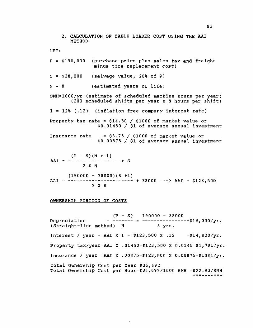
2. CALCULATION OF CABLE LOADER COST USING THE AAIMETHOD
LET:
SMH=1600/yr.(estimate of scheduled machine hours per year)(200 scheduled shifts per year X 8 hours per shift)
I = 12% (.12) (inflation free company interest rate)
Property tax rate = $14.50 / $1000 of market value or$0.01450 / $1 of average annual investment
Insurance rate $8.75 / $1000 of market value or$0.00875 / $1 of average annual investment
(P - S)(N + 1)AAI= +s
2 XN
(190000 - 38000)(8 +1)+ 38000 ===> AAI = $123,500AAI =
2X8
OWNERSHIP PORTION OF COSTS
83
Interest / year = AAI X I = $123,500 X .12 =$14,820/yr.
Property tax/year=AAI X .01450=$123,500 X 0.0145$1,791/yr.
Insurance / year =AAI X .00875=$123,500 X O.00875$1081/yr.
Total Ownership Cost per Year=$36,692Total Ownership Cost per Hour=$36,692/1600 SMH $22.93/SMH
P = $190,000 (purchase price plus sales tax and freightminus tire replacement cost)
S = $38,000 (salvage value, 20% of P)
N = 8 (estimated years of life)
(P - S) 190000 - 38000Depreciation = $19, 000/yr.(Straight-line method) N 8 yrs.

Tire Replacement CostEstimated life (SMH) 3000
--- =$3.00/SMH
Total Equipment Cost (Ownership + Operating) = $33.69ISMH
For each hour the loader is scheduled to work, it mustrecover $33.69 to break even. This is also the hourlyamount a crew on incentives would be charged to use thisloader. A daily rate could also be determined usingthis cost.
84
OPERATING PORTION OF COSTS
Repair and Maintenance (50% of depreciation)Repair and Maintenance = $19,000 X .50 = $9,500 I yr.
$9,500 I 1600 SMH = $5.94 I SMH
Fuel Consumption=2 gallons per machine hour. Assume loaderworks 7.5 hours per Echeduled 8 hour day.
2 gallons 7.5 machine hours of workX -1.9 gallons I SMH
machine hour 8 scheduled machine hours
1.9 gallons I SMH X 1600 SMH Iyear = 3040 gallons I year3040 gallonE I year X $0.80 I gallon = $2,432 I year
1.9 gallons I SMH X $0.80 I gallon = $1.52 I SMH
Lube and Oil=$0.20/$l of fuel=.20 X $2,432/yr.=$486 I year$0.20 I $1 of fuel = .20 X $1.52 = $.30 I SMH
Subtotal Operating Costs per Year = $12,418 Iyr.Subtotal Operating Costs per Hour= $12,418
= $7.76 I SMH1600 SMH
Replacement cost $10,000
Total Operating Cost = $10 .76/SMH

85
3. EXAMPLE CALCULATION USING THE MARGINAL COST METHOD(NEXT YEAR'S ACTUAL COST)
Assume the loader in the previous example is being
used in year nine. Since the loader was previously
costed using an estimated life of eight years, it is
incorrect to continue to use the AAI method of cost
calculation. The average annual investment now becomes
the current market value of the piece of equipment. For
simplicity of calculation, the market value should be
the fair market value at the start of the year and may
include any value for tire, tracks, and wire rope.
Also, since the piece of equipment has been depreciated
over eight years, there would be no depreciation charges
when a marginal cost method is used.
Example:
Let the current market value (MV) = $40,000 (includestires and wire rope)
SMH = 1600/yr. (estimate of scheduled machine hours peryear; 200 scheduled shifts per yearX 8 hours per shift)
I = 12% (.12) (company interest rate, or MARR)
Property tax rate = $14.50 / $1000 of market value or$.01450 / $1 of average annualinvestment
Insurance rate = $8.75 / $1000 of market value or$.00875 / $1 of average annualinvestment

86
OWNERSHIP PORTION OF COSTS
Depreciation (equipment has been depreciated) = $0 I yr.
Interest I year = MV X I = $40,000 X .12 =$4,800/ yr.
Property tax/year=MV X .01450 $40,000 X 0.0145= $580 I y.
Insurance I year =MV X .00875=$40,000 X 0.00875= $350 I yr.
Total Ownership Cost per Year = $5,730Total Ownership Cost per Hour = $5,730/1600 SMH=$3.59 I SMH
Note that when switching from the AAI method to themarginal cost method, the ownership cost decreases from$22.93 / SMH to $3.59 / 5MM. This difference becomessignificant when planning bids on timber sales or whencharging a crew for a piece of equipment.
OPERATING PORTION OF COSTS
Repair and Maintenance (estimate of actual cost)=$15,000/yr.$15,000 / 1600 SMH = $9.38/SMH
Fuel Consumption=2 gallons per machine hour. Assume loaderworks 7.5 hours per scheduled 8 hour day.
2 gallons 7.5 machine hours of workX = 1.9 gallons/SMH
machine hour 8 scheduled machine hours
1.9 gallons / 5MM X 1600 SMH /year = 3040 gallons/year3040 gallons / year X $0.80 / gallon = $2,432/year
1.9 gallons / SMH X $0.80 / gallon = $1.52/SMH
Lube and Oil=$0.20 / $1 of fuel=.20 X $2,432 /yr.=$486/year$0.20 / $1 of fuel = .20 X $1.52 =$.30/SMH
Operating Costs per Year = $17,918/yrOperating Costs per Hour = $17,918 / 1600 SMH = $11.20/SMH
Tire and wire rope replacement costs have been includedin the current market value using this method. As anoption, these items can be costed out separately.Appendix E shows an example of estimating wire rope costbased on production.
Total equipment cost (Ownership + Operating)= $23,648/year$23,648 / 1600 SMH = $14.78/SMH
Note that the total equipment cost using the AAI method is$33.69/SMH while the marginal cost method is $14.78/SMH.

4. EXAMPLE OF INFLATINC EQUIPMENT COSTS
Assume that the cable loader costed in part 2 wasfor base year 1987. The loader will be used in 1988.To account for inflation, the 1987 base year cost shouldbe inflated.
INFLATING OWNERSHIP COSTS
Assume:General inflation rate = 6% (0.06) (estimate for 1988)
Inflate the ownership cost as follows:
ownership cost (current year) X (1 + general inflation rate)= ownership cost (next year)
22.93 / hr. X (1 + 0.06) = $24.31 / hr.
INFLATING OPERATING COSTS
Repair and Maintenance (inflate 6% (0.06))
$9,500 (1987) / year X (1 + 0.06) = $10,070 / year (1988)$5.94 (1987)! SMH X (1 + 0.06) = $6.30 / SMH (1988)
Fuel Consumption = 2 gallons per machine hour. Assumeloader works 7.5 hours per scheduled8 hour day. Estimated fuel cost(1988) = $0.85 / gallon.
2 gallons 7.5 machine hours of workX = 1.9 gallons/SMH
machine hour 8 scheduled machine hours
1.9 gallons / SMH X 1600 SMH /year = 3040 gallons/year3040 gallons / year X $0.85 / gallon = $2,584/year
1.9 gallons / SMH X $0.85 / gallon = $1.62/SMH
Lube and Oil=$0.20/$1 of fuel=.20 X $2,584 /yr.=$517/year$0.20 / $1 of fuel= .20 X $1.62 = $.32 / SMH
Subtotal Operating Costs per Year = $13,171 / yrSubtotal Operating Costs per Hour=$13,171/1600 SMH=$8.23/SMH
Replacement cost $10,500Tire Replacement Cost- = =$3.50/SMH(1988 estimated cost) Estimated life (SMH) 3000
Total Operating Cost = $11.73/SMH
87
Total cost (ownership plus operating) = $36.04/SMH
Note that inflation causes an increase of $2.35/SMH($33.69/SMH (1987) versus $36.04/SMH (1988).

APPENDIX D
1. OWNERSHIP PERIOD GUIDE
88

TABLE Dl.
GUIDE FOR SELECTING OWNERSHIP PERIOD BASED ON APPLICATION AND OPERATING
CONDITIONS.
Intermittent full throttle
operation.
No impact.
Pulling scrapers, most
agricultural drawbar,
stockpile, and landfill
work.
Intermittent skidding for
short distances, no
decking.
Good underfoot
conditions:
level terrain,
dry floor, few if any
stumps. 12,000
Hours
Well maintained haul roads.
Construction use mostly on
well maintained roads.
25,000
Hours
Medium impact conditons.
Production dozing in clays,
sands, gravels.
Most land
clearing and skidding
applications.
Continuous turning, steady
skidding for medium dis-
tances with moderate deck-
ing.
Good underfooting:
dry floor with few stumps
and gradual rolling terrain
10,000
Hours
Varying loading and haul
road conditions.
Typical
road-building use on a
variety of jobs.
20,000
Hours
Continuous high impact
conditions.
Heavy rock
ripping.
Pushloading and
dozing in hard rock.
Tandem ripping.
Continuous turning, steady
skidding for long dis-
tances with frequent deck-
ing.
Poor underfoot con-
ditions:
wet floor, steep
slopes, numerous stunps.
8,000
Hours
Consistently poor haul
road conditions. Extreme
overloading.
Oversized
loading equipment.
15,000
Hours
TPACK-TYPE
TPACTORS
Sma 11
Large
EEL
SI(IDDERS
Of f Highway
Trucks and
Tractors Adapted from the Caterpillar Performance Handbook
See note on ownership guide, page 91.
12,000
Hours
10,000
Hours
8,000
Hours
22,000
Hours
18,000
Hours
15,000
Hours

TA
BL
E D
2.G
UID
E F
OR
SE
LE
CT
ING
OW
NE
RSH
IP P
ER
IOD
BA
SED
ON
APP
LIC
AT
ION
AN
D O
PER
AT
ING
CO
ND
ITIO
NS.
Inte
rmitt
ent t
ruck
load
ing
from
sto
ckpi
le.
Free
flo
w-
ing,
low
den
sity
mat
eria
ls.
Lig
ht s
now
plow
ing.
Loa
dan
d ca
rry
on g
ood
surf
ace
for
shor
t dis
tanc
es w
ithno
gra
des.
Inte
rmitt
ent t
ruck
load
ing
from
sto
ckpi
le.
Min
imum
trav
elin
g, tu
rnin
g.Fr
eefl
owin
g, lo
w d
ensi
ty m
at-
eria
ls w
ith s
tand
ard
buc-
ket.
No
impa
ct.
12,0
00 H
ours
Lig
ht r
oad
mai
nten
ance
.L
ight
sno
w p
low
ing.
Lar
geam
ount
s of
trav
elin
g.
20,0
00H
ours
Con
tinuo
us tr
uck
load
ing
from
sto
ckpi
le.
Low
tom
ediu
m d
ensi
ty m
ater
ials
in p
rope
rly
size
d bu
cket
.L
oadi
ng f
rom
ban
k in
goo
ddi
ggin
g.L
oad
and
carr
y on
poor
sur
face
s an
d sl
ight
adve
rse
grad
es.
Ban
k ex
cava
tion,
inte
rmit-
tent
rip
ping
, bas
emen
t dig
-gi
ng o
f na
tura
l cla
ys,
sand
s, s
ilts,
gra
vels
.So
me
trav
elin
g.St
eady
full
thro
ttle
oper
atio
n.
10,0
00H
ours
Hau
l roa
d m
aint
enan
ce.
Roa
d co
nstr
uctio
n, d
itch-
ing.
Med
ium
to h
eavy
sno
wre
mov
al. 15,0
00H
ours
Loa
ding
sho
t roc
k (l
arge
load
ers)
.H
andl
ing
high
dens
ity m
ater
ials
with
coun
terw
eigh
ted
mac
hine
.St
eay
load
ing
from
ver
ytig
ht b
ank.
Con
tinuo
usw
ork
on r
ough
or
very
sof
tsu
rfac
es.
Con
tinuo
us w
ork
on r
ock
surf
aces
.L
arge
ani
ount
of
ripp
ing
of ti
ght,
rock
ym
ater
ials
.H
igh
impa
ctco
nditi
ons.
8,00
0H
ours
Mai
nten
ance
of
hard
pac
kro
ads
with
err
edde
d ro
ck.
Con
tinuo
us h
igh
load
fact
or.
Hig
h im
pact
.
12,0
00H
ours
WH
EE
LL
OA
DE
RS
TR
AC
K-T
YPE
LO
AD
ER
S
MO
TO
RG
RA
DE
RS
Ada
pted
fro
m th
e C
ater
pilla
r Pe
rfor
man
ce H
andb
ook
See
note
on
owne
rshi
p gu
ide,
pag
e 91
12,0
00H
ours
10,0
00H
ours
8,00
0H
ours
15,0
00H
ours
12,0
00H
ours
10,0
00H
ours
Smal
l
Lar
ge
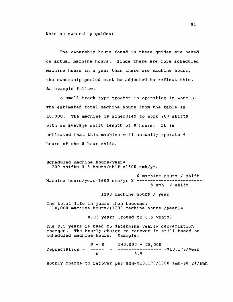
Note on ownership guides:
The ownership hours found in these guides are based
on actual machine hours. Since there are more scheduled
machine hours in a year than there are machine hours,
the ownership period must be adjusted to reflect this.
An example follow.
A small track-type tractor is operating in Zone B.
The estimated total machine hours from the table is
10,000. The machine is scheduled to work 200 shifts
with an average shift length of 8 hours. It is
estimated that this machine will actually operate 6
hours of the 8 hour shift.
Scheduled machine hours/year=200 shifts X 8 hours/shift=1600 smh/yr.
6 machine hours I shiftMachine hours/year=1600 smh/yr X =
8 smh I shift
1200 machine hours I year
The total life in years then becomes:10,000 machine hours/(1200 machine hours Iyear)=
8.33 years (round to 8.5 years)
The 8.5 years is used to determine yearly depreciationcharges. The hourly charge to recover is still based onscheduled machine hours. Example:
P - 5 140,000 - 28,000Depreciation = = =$13,176/year
N 8.5
91
Hourly charge to recover per SMH=$13,176/1600 smh=$8.24/smh

APPENDIX E
1. CONVERTING WIRE ROPE LIFE BASED ON PRODUCTIONTO LIFE IN HOURS.
92

CONVERTING WIRE ROPE LIFEBASED ON PRODUCTION TO LIFE IN HOURS
To convert an estimate of wire rope life from totalproduction to scheduled machine hours, the followingparameters must be known:
Gross MBF (or other measure) produced between wire ropereplacement.
An estimate of average production (gross MBF) per day.
The average scheduled hours per shift.
As an example, assume the following:
Gross MEF produced between replacement = 6000 MBFGross MEF produced per day (estimated) = 40 MEF / dayAverage scheduled hours per shift = 8.5 hrs
The number of days between replacement =
6000 MEF / (40 MBF/day) = 150 days
The number of scheduled hours between replacement =
150 days X 8.5 hours/day = 1275 scheduled machine hours
To determine the cost of line replacement, the followingmust be known:
Total wire rope length to be replaced.
Price per unit length of wire rope.
As an example, assume the following:
Total wire rope length = 2500 feetPrice per foot of wire rope = $1.34 / foot
The total cost of wire rope replacement is:
2500 feet X $1.34 / foot = $3350
The cost per scheduled machine hour for wire ropereplacement becomes:
$3350 / 1275 SMH = $2.63 / SMH
93

APPENDIX F
1.BRIEF DESCRIPTION OF MONETARY INCENTIVE PROGRAMS
94

95
1. BRIEF DESCRIPTION OF MONETARY INCENTIVE PROGRAMS
Monetary incentive programs can be summarized in
two general forms. One form negotiates a price, or
"cost goal", to do a job. The job can be anything from
road construction to yarding and loading a logging
setting or unit. The price negotiated is usually stated
in a price per unit of production, such as $/MBF or
$/station. A pool of money is then generated by the
crew by multiplying the contract rate per unit of
production by the units produced. From this crew
"revenue" pool expenses such as labor costs, equipment
costs, penalties for safety or quality infractions, and
administration costs are subtracted. The money
remaining after subtracting all crew costs from the crew
revenue is the bonus pools This bonus pool is
distributed among the crew in a variety of combinations.
The crew may receive 100% of the bonus or they may get
as low as a 50%-50% split with the company.
Another form of monetary incentives gives an increase
in wages for an increase in a target production level.
For example, if a target level of 1 MBF/man-hour was set
and actual production of 1.1 MBF/man-hour was reached,
actual production would be 10% higher than the target
production. Wages would be increased by 10% as a result.
Additional information on these incentive programs
and the subsequent distribution of the bonus pool is
available In the paper "Loin Incentive Systems"
(Olsen, 1987).
APPENDIX G
1. AN OVERVIEW OF OREGON'S WORKERS' COMPENSATIONSYSTEM
96
97
AN OVERVIEW OF OREGON'S WORKERS' COMPENSATION SYSTEM
An overview of Oregon's Workers' Compensation
system requires a description of the different agencies
involved and the roles they play.
State Leqislature:Makes and ammends the laws governing the system.Establishes the benefit levels for injured workers.
Governor:Signs legislative measures into law.
Workers' Compensation DeDartment (WCD):Responsible for the enforcement and regulation ofOregon's Workers' Compensation Law.
Workers' Compensation Board (WCB):Provides for the settlement and disposition ofcontested claims.
National Council on Compensation Insurance (NCCI):A national rate-making organization, providesstatistics to help insurance carriers set rates forjob classifications. The Oregon Council onCompensation Insurance COCCI) is an affiliate of NCII.
Oreqon Insurance Commissioner:Regulates activities of Oregon's insurance carriers.
Insurance carriers:Ultimately set rates for job classifications based onthe information provided by NCCI and OCCI. Providescoverage to employers and benefits to workers.
The calculation of insurance rates for Workers'
Compensation is complicated at best. However,
understanding the basics of rate setting is vital to
good cost records. The National Council on Compensation
Insurance isa national rating organization. They
collect detailed payroll and claims statistics annually

98
from insurance carriers and use this information to
develop annual "pure" premium rates. Pure premium rates
are limited to what is required to pay claims and
exclude consideration of administration expenses by
individual insurance carriers. Rates differ by industry
classification, according to the relative hazards of
each.
Individual insurance companies modify the rates
given by NCCI to cover administrative and business
expenses. The rates for Oregon carriers can be twenty-
five percent greater than those established by NCCI.
Rates are based on a dollar per 100 dollars of payroll.
For example, the rate for logging in Oregon is
approximately $27 per $100 of payroll (1986 figure).
This means that claims in the logging classification
will average a total of $27 for each $100 of payroll.
The cost of claims is transferred directly to the
insured in the form of premiums. For each $100 of
payroll in the logging classification, $27 of premium
will be paid by the logging company.
Classification rates vary for each insurance
carrier, but this variation will be slight since pure
rates are set by NCCI and individual carriers wish to
remain competitive. Some insurance carriers have a
preferred rate which can further reduce the
classification rates up to 10%. These preferred rates
are given to companies that consistently have good
99
safety records and pay over a certain amount in premiums
each year. Classification rates are updated annually by
NCCI and take effect on 3anuary 1. The insured company
may have a premium period which is different than
3anuary 1 to December 31. In this case, the rates in
effect at the time of the premium renewal last for the
entire premium period. A revised rate is assigned at
the start of the next premium period.
The classification rates go through four
adjustments before a final premium is reached. These
four adjustments are: an adjustment for experience
modification, a premium discount, a Workers'
Compensation Department tax, and a workday tax. Each of
these four adjustments will be discussed in detail.
Experience modification--The experience modification,
also known as experience rating, is a means in which the
manual rates for job classifications can be adjusted to
reflect an individual company's loss expectations. The
manual rate is a job classification average, most
companies will not have claims that equal this average.
To reflect this deviation from the average, the manual
rates are modified based on the actual claims
characteristics of the insured. If the insured has
lower actual losses than expected, the manual rates are
adjusted downward. If the insured has higher actual
losses than expected, the manual rates are adjusted
100
upward. The actual and expected losses of an Insured
company is calculated by NCCI over a base period of
time, usually three years.
Since the experience modification is being
calculated during the current policy period the
experience period is actually the first three of the
last four years. For example, the experience rating for
policy year 1987 would be calculated from company claims
statistics for 1983, 1984, and 1985. For policy year
1988, the claims statistics for 1984, 1985, and 1986
would be used. Another important feature of the
experience modification is that NCCI weights the
frequency of accidents higher than the severity. This
means that a company with fewer costly accidents may
have a higher experience modification than a company
with one or two severe accidents.
There are several ramifications of which to be
aware when considering experience modification and
monetary incentive programs. First, the experience
modification is determined from a base period of the
first three of the last four years as discussed above.
This means that a company that had one or two bad safety
years in the past four years could still have a high
experience rating even though the current crew (who may
be all new employees) has a very good safety record.
Second, the experience rating is determined for the
company as a whole. Individual crews are not

considered. A safe crew could be paying for the
accidents or unsafe actions of another crew.
There is no easy solution to this problem with the
way the current Workers' Compensation system is set up.
A company with several crews may need to set up a system
of deducting an amount of a crew's incentive pay based
on the frequency of accidents. Also, a well
administered monetary incentive program should not
result in an increase in accidents. It's important that
the members of the yarding and loading crew be aware of
how this experience modification is set and how safe
working practices can bring the cost of Workers'
Compensation down while increasing the amount of
incentive pay available.
Premium discount--A discount will be applied to the
premium after it has been adjusted for experience
modification. The discounts are based on the amount of
expected annual adjusted premium paid during a policy
year. No discount applies to the first $2,500 of annual
premium. For 1986, the premium discounts are as
follows:
AMOUNT OF ADJUSTED PREMIUM PERCENT DISCOUNT
$2,501 to $10,000 6%$10,001 to $30,000 10%$30,001 to $50,000 12%
$50, 001+ 14%

102
Workers' Compensation Department tax--A tax is applied
to the net premium (the experience modification premium
minus the premium discount). This tax is used to cover
the administrative costs of the Workers' Compensation
Department and the Workers' Compensation Board. The tax
rate is set by the state legislature and is the same for
all companies. The rate remains in effect for the
entire policy period. For 1986, the WCD tax rate was
12% of the net premium.
Workday tax--For each day or part day worked by each
employee, a tax is assessed. Since January 1, 1984, a
tax of $26 per full day or part day worked per employee
has been assessed. Fourteen cents is contributed by the
worker while the remaining $.12 is contributed by the
employer. ThiE tax IE uEed to support the Handicapped
Workers' Reserve Fund, the Workers' Re-employment
Reserve Fund, and the Retroactive Reserve Fund.

APPENDIX H
1. ASSESSING SAFETY AND QUALITY INFRACTIONS IN AMONETARY INCENTIVE PROGRAM
103

ASSESSING SAFETY AND QUALITY INFRACTIONS
A properly administered monetary incentive program
must have the means to maintain safety and quality
standards at a desired level. Without control over
these items the cost of logging could increase as
Workers' Compensation premiums rise due to an increased
accident rate or as logging contracts become harder to
obtain due to a reputation of a poor quality job.
Quality involves both log quality (logs manufactured to
purchasers' specifications) and contract compliance
quality (proper utilization and environmental quality
such as brush disposal and erosion control).
METHODS CURRENTLY BEING USED-- There are methods being
used to insure safety and quality are maintained within
the framework of a monetary incentive program.
Safety--The contract rate negotiated to do a job is
always calculated with safety in mind. The rate is
based on a production amount that the crew can reach
while working in a safe manner. Administrative controls
are often used to maintain safety standards. This
involves the logging foreman or supervisor talking to
the crew, identifying the problem, and having both the
crew and company, if necessary, take corrective action
to eliminate the problem. If the problem persists,
104
105
other actions such as dismissal of employees may become
necessary. In combination with administrative controls,
there are several methods used that penalizes the crew
monetarily for safety infractions. If the cost of
Workers' Compensation increases this cost is passed on
to the crew in the form of a higher labor burden. This
can decrease the amount of bonus pool that is available
to the crew.
Unfortunately, the Workers' Compensation experience
rating is set yearly and is based on the first three of
the last four years, as discussed in the section on
Workers' Compensation. A more immediate penalty is
often assessed in addition to this future increase in
the labor cost. These penalties often take the form of
a monetary decrease in the bonus pool. The decrease is
often a percent decrease for each reportable accident.
For example, a five percent decrease in the bonus pool
may be assessed for each reportable accident.
There are other methods of controlling safety which
are outside the scope of this report. These methods
involve specific safety incentive programs which may or
may not be used in conjunction with productivity
incentive programs. However, the general consensus
among industries presently using monetary incentive
programs is that safety does not deteriorate when a crew
is placed on a properly administered program.

106
Loq quality--It is not difficult for a logging
contractor to know the specifications that a mill or
purchaser requires for delivered logs. These
specifications can then be reflected in the contract
rate negotiated for the incentive unit. If log quality
is not met, there are several options that can be used
to bring quality up to standards. The first option
would be to use administrative controls much like those
used for safety infractions. The administrator of the
operation must be able to identify whether the log
quality is not being met due to the falling and bucking
crew or the yarding and loading crew. In most cases a
few inspections In the field will reveal the source of
the problem. If administrative controls are not
adequate to bring log quality up to standard, then a
penalty is usually assessed. This can take the form of
a reduction in the bonus pool of anywhere from one
percent to five percent.
Another option that may be viable in some logging
contracts is to pass any monetary penalties assessed
against a logging company back to the crew that caused
the penalty. Many mills now have some sort of log
quality program which assess a penalty or gives a bonus
depending on the level of log quality met. The
penalty/bonus is usually calculated on a $/MBF basis for
the volume delivered in a one month period. It may not

107
be possible to track the monthly volume to a particular
unit but the sale, and in most cases the crew, can be
tracked. The penalty/bonus should be passed on as
quickly as possible and this can be given to the crew as
an increase or decrease in the amount of bonus pool made
available.
Compliance work quality--In the case of monetary
incentive programs, compliance work quality infractions
must pertain only to that work required of the incentive
crew.
Cable yardinq crews--Typically, the only compliance work
a cable-logging crew is responsible for is YUM yarding
(yarding unutilizable material) and streamcourse
cleanout (removing larqe woody material inadvertently
placed in a stream during logging). These two work
items need to done in conjunction with the yarding of
merchantable material to avoid the cost of moving in and
setting up a separate yarder. Fortunately, these two
items are typically the only ones required of a cable
logging crew so it is relatively easy to control the
quality of these items. Since YUM yarding and
streamcourse cleanout are known in advance, these items
should be included in the price negotiated for the unit.
Failure to complete these items to standard can then be
handled administratively or with a monetary penalty as
108
discussed in the previous sections. Another control an
administrator of the operation can have for these
quality items is to require the work to be completed
before the crew moves to a new unit. This essentially
"forces" the crew to keep current with the compliance
work required.
Ground-based yardinq crews--The compliance work required
of ground based crews is typically more involved than
that required of cable crews. In addition to YUM
yarding and streamcourse cleanout, items such as brush
piling and erosion control work (water barring, erosion
control grass seeding, scarification of roads and skid
trails) is also required. Typically, a ground-based
logging operation will have one crawler piling brush
concurrent with the skidding operation. The brush
piling may or may not be in the same unit as the
skidding operation. YUMing may take place concurrent
with the skidding although it is not uncommon for one or
two skidding machines to YUM an area after the
merchantable material has been removed.
These compliance work situations are more difficult
to include in an incentive program than those required
of cable yarding crews. If a contractor has good
production records for compliance work, it would be
possible to include the compliance work with the
skidding of merchantable material. The cost goal would

109
include the cost of compliance work. The contract would
have to include provisions for keeping the work current.
An amount of money could be held out of the final
settlement until the compliance work was completed. As
an alternative to holding money out of the compliance
settlement, a contractor may elect to declare a unit
complete once all compliance items have been accepted.
If a contractor does not have good compliance
production records, an option would be to treat some of
the compliance work as a separate job. For example, the
brush piling and any erosion control work such as
scarification and water barring might be kept as a
separate job. Yarding of unutilizable material could be
included with the skidding of merchantable logs, the
same as with cable crews. If the compliance crew spends
any time skidding logs, those hours for labor and
equipment would be charged against the operation.