determining optimal strategies in matrix gamesmdv/courses/cm30082/projects.bho/2006-7/patel... ·...
TRANSCRIPT

Determining Optimal Strategies in Matrix Games
Hemal Ramesh Patel
Bachelor of Science in Computer Information Systems with Honours
The University of Bath May 2007

Determining Optimal Strategies in Matrix Games
i
This dissertation may be made available for consultation within the University Library and may be photocopied or lent to other libraries for the purposes of consultation. Signed: Hemal Patel

Determining Optimal Strategies in Matrix Games
ii
Determining Optimal Strategies in Matrix Games
Submitted by: Hemal Ramesh Patel
COPYRIGHT
Attention is drawn to the fact that copyright of this dissertation rests with its author. The Intellectual Property Rights of the products produced as part of the project belong to the University of Bath (see http://www.bath.ac.uk/ordinances/#intelprop).
This copy of the dissertation has been supplied on condition that anyone who consults it is understood to recognise that its copyright rests with its author and that no quotation from the dissertation and no information derived from it may be published without the prior written consent of the author.
Declaration
This dissertation is submitted to the University of Bath in accordance with the requirements of the degree of Bachelor of Science in the Department of Computer Science. No portion of the work in this dissertation has been submitted in support of an application for any other degree or qualification of this or any other university or institution of learning. Except where specifically acknowledged, it is the work of the author.
Signed: Hemal Patel

Determining Optimal Strategies in Matrix Games
iii
Abstract
The origin of game theory can be traced back to the 18th century, but the development of the topic began with the works of John Von Neuman, Oskar
Morgenstern and John Forbes Nash Jr. This dissertation looks at the history of game theory and applications in today’s world. Depth into solving Zero-Sum Two Person Matrix Games are investigated and implemented.

Determining Optimal Strategies in Matrix Games
iv

Determining Optimal Strategies in Matrix Games
v

Determining Optimal Strategies in Matrix Games
vi
APPENDIX A – GLOSSARY 71.
APPENDIX B – LINEAR ALGEBRA 73.
APPENDIX C - SOURCE CODE 75.
APPENDIX D – TEST CASES 87.
APPENDIX E – TEST DATA 108.
APPENDIX F – RAW RESULTS OUTPUT 143.
APPENDIX G - ADDITIONAL TESTING 169.

Determining Optimal Strategies in Matrix Games
vii
List of Figures

Determining Optimal Strategies in Matrix Games
viii
Determining Optimal Strategies in Matrix Games
ix
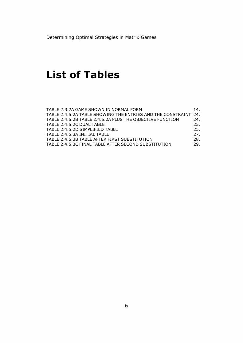
List of Tables
TABLE 2.3.2A GAME SHOWN IN NORMAL FORM 14. TABLE 2.4.5.2A TABLE SHOWING THE ENTRIES AND THE CONSTRAINT 24. TABLE 2.4.5.2B TABLE 2.4.5.2A PLUS THE OBJECTIVE FUNCTION 24.
TABLE 2.4.5.2C DUAL TABLE 25. TABLE 2.4.5.2D SIMPLIFIED TABLE 25. TABLE 2.4.5.3A INITIAL TABLE 27.
TABLE 2.4.5.3B TABLE AFTER FIRST SUBSTITUTION 28. TABLE 2.4.5.3C FINAL TABLE AFTER SECOND SUBSTITUTION 29.

Determining Optimal Strategies in Matrix Games
x
Acknowledgements
I would like to acknowledge my project supervisor, Professor Nicolai Vorobjov for his valuable and constant assistance throughout the lifecycle of this dissertation.
I would also like to give thanks to Richard Walklate and David Murrant for their assistance. Finally I would like to thank my family, especially my mother, for her constant support and encouragement throughout my educational life.

Determining Optimal Strategies in Matrix Games
11
Chapter 1
Introduction
Games are defined as a competitive activity involving skill, chance, or endurance on the part of two or more persons who play according to a set of rules, usually
for their own amusement or for that of spectators. Games could be in the form of physical activity such as sports or mental activity such as parlour games. The common characteristic of all games is that
players will have a strategy that they intend to follow through. The strategies that the players will adopt will depend on the skill of the player or random chance/luck. Take three parlour games; chess, poker and roulette. These types of
games do vary with the application of chance and skill, therefore altering the strategies that the players adopt. In the game of chess, chance or luck does not exist as the moves are
skilfully thought through and planned ahead to devise a checkmate. Poker combines chance and skill, as the cards that a player will play with, will depend on the “hand” of the player and the other players’ cards. The game of roulette is a game of chance where skill plays no part.
Common with all games is the amount of knowledge available to the players. The knowledge that the players have can assist in determining the strategies that they can adopt. In the game of chess, knowledge is perfect as the moves that the players have made are known throughout the game. The
strategies adopted by the players can complement the knowledge that they have. Poker unlike chess has imperfect knowledge because the player will not
know the deck of the opponents and therefore the strategy will be based on the cards that the player holds. The main objective of all games is to win and in particular to maximise the win. Winning could be in the form of pride, trophies or money. In order to
win at any game the players of the game will have to find and play their best strategies.

Determining Optimal Strategies in Matrix Games
12
The strategy in games is studied in a field of mathematics and economics and is known as Game Theory. Game theory will be the chosen domain for this dissertation.
The aims of the project are to research into the topic of Game Theory and design and implement an application to determine strategies and payoffs for players, for a given game. The project dissertation will be split into several sections.
The first section will contain the literature review, which will provide the foundation of the project and research into the existing solutions of the problem. Following the literature review will be the requirements section, which will formally specify the functionality of the application. Leading the requirements
will be the design section. This section will discuss the algorithms needed to solve the problem. The implementation section will discuss the implementation of the algorithms mentioned in the design section. The next section will be the testing, which will detail the testing of the application. The project dissertation
will conclude with the conclusion. The appendix will contain the source code and test data for the application.
Attached along with the dissertation will be a CD containing all of the code.

Determining Optimal Strategies in Matrix Games
13
Chapter 2
Literature Survey
2.1. Introduction The purpose of this literature review is to investigate the topic of game theory.
The topic needs to be fully understood, from what the topic briefly is, how it has evolved, who uses game theory and its applications. Dawson (2000) states that the literature review process, serves the following purposes;
� It justifies the project such that it shows that the project is worth doing and the area being investigated, in this case Game Theory, is recognised and meaningful.
� It sets the project within context by analysing past and current research
in the chosen area. Through this, the identification of how the project fits within and contributes to area is determined.
� It allows other researchers to use the work done on the project, for their
own research purposes and continue where the project left off. The literature review will follow the structure of an overview to what game theory is from a brief history, the applications of game theory and representation
of games, to the computation of optimal strategies in particular types of games. Concluding the literature review will be a summary.
2.2. Game Theory
2.2.1 What is Game Theory? Game Theory is how decision makers interact with each other in a competitive
sense and the process they take in making a rational/strategic choice (Osborne 2004) and a choice that is the best response to the other player’s strategy (McCain 2004).

Determining Optimal Strategies in Matrix Games
14
2.2.2 Brief History of Game Theory Early parts of game theory can be traced back to the 18th century, however
game theory went through major developments in the early part of the 20th century, which lead to a book being written by one of the “godfathers” of game theory, mathematician John Von Neumann. His book was called, Theory of Games and Economic Behaviour (Osborne 2004).
In 2001 the game theory was glamorised by the red carpets of Hollywood, as the film, A Beautiful Mind that starred Russell Crowe as the economist John Forbes Nash (McCain 2004), who in the 1950’s:
“developed a key concept (Nash Equilibrium) and initiated
the game-theoretic study of bargaining” – Osborne (2004, p2).
2.2.3 Applications Game theory is often described as a branch of applied mathematics and
economics. However game theory has got an interest in vast amounts of academic subjects. This ranges from Biology to Sociology and also including Computer Science (Wikipedia 2006 and McCain 2004). Computer scientists are interested in game theory, as game theory has
got important links with logic and several logical theories have a basis in game semantics (Wikipedia 2006). Game theory also has a wide range of applications from business,
auctions, military, political and more famously gambling (McCain 2004 and Osborne 2004).
2.3. Games and Representation of Games
2.3.1 Definition of Games According to sources, Owen (1982) and Osborne (2004) the definition of a game consists of; a set of players, the strategies/choices that they have available to
them and a payoff table/preference. The payoff for the strategies could either be in the form of money or pride etc…
2.3.2 Normal and Extensive Form of Games
Table 2.3.2a Game shown in Normal Form

Determining Optimal Strategies in Matrix Games
15
Game theory has two common ways of representing games; either in table format (Normal Form (Table 2.3.2a)) or in tree format (Extensive Form (Figure 2.3.2a)).
Figure 2.3.2a and Table 2.3.2a are representations of the game
Prisoner’s Dilemma (McCain 2004). From those representations, it can be deduced that the strategies of games can be written in a matrix. This is also supported by Owen (1982).
The individual elements within the matrix represent the payoff for undertaking a certain strategy. Also for choosing a particular strategy, there is a probability that the strategy will and will not work. This is taken into account in the payoff. During a game, players may sometimes try to reduce the payoff
amount that they have to pay. This is called the minimax theorem. This can be also seen as maximising the minimum gain (Owen 1982).
2.3.3 Zero-Sum Games Matrix games can come in various forms, from symmetric and asymmetric to
zero and non-zero-sum games (Osborne 2004).
Figure 2.3.2a Game shown in Extensive Form
Figure 2.3.2b A Matrix
Figure 2.3.3a Zero-Sum Matrix Game
Determining Optimal Strategies in Matrix Games
16
Owen (1982) and McCain (2004) both state that zero-sum matrix games are games such that the payoff inside the matrix, adds up to zero. Figure 2.3.3a shows this, as within each cell, the payoff adds up to zero.
2.4. Computation of Optimal Strategies
Owen (1982) states that due to the minimax theorem, in every two person zero-sum matrix game, optimal strategies will exist.
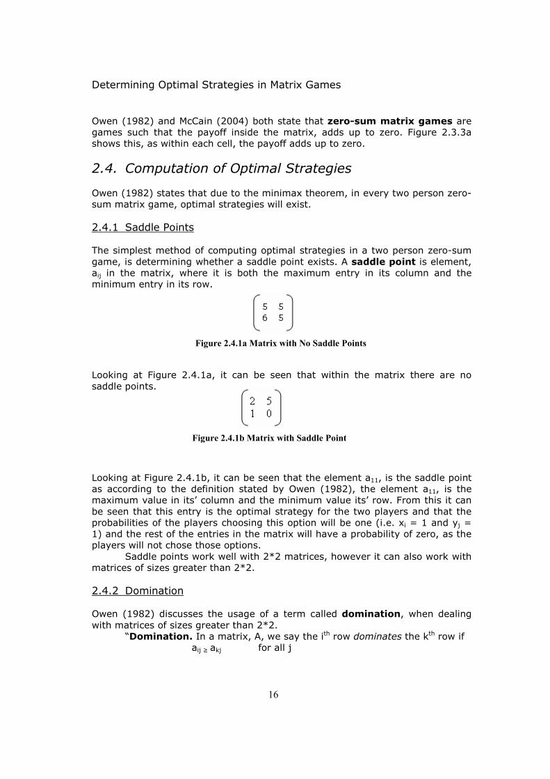
2.4.1 Saddle Points The simplest method of computing optimal strategies in a two person zero-sum
game, is determining whether a saddle point exists. A saddle point is element, aij in the matrix, where it is both the maximum entry in its column and the minimum entry in its row.
Looking at Figure 2.4.1a, it can be seen that within the matrix there are no
saddle points.
Looking at Figure 2.4.1b, it can be seen that the element a11, is the saddle point as according to the definition stated by Owen (1982), the element a11, is the maximum value in its’ column and the minimum value its’ row. From this it can
be seen that this entry is the optimal strategy for the two players and that the probabilities of the players choosing this option will be one (i.e. xi = 1 and yj = 1) and the rest of the entries in the matrix will have a probability of zero, as the players will not chose those options.
Saddle points work well with 2*2 matrices, however it can also work with matrices of sizes greater than 2*2.
2.4.2 Domination Owen (1982) discusses the usage of a term called domination, when dealing
with matrices of sizes greater than 2*2. “Domination. In a matrix, A, we say the ith row dominates the kth row if
aij ≥ akj for all j
Figure 2.4.1a Matrix with No Saddle Points
Figure 2.4.1b Matrix with Saddle Point

Determining Optimal Strategies in Matrix Games
17
And aij ≥ akj for at least one j
Similarly, we say the jth row dominates the lth row if aij ≥ ail for all i
And aij ≥ ail for at least one i” (Owen 1982, pp.22-23)
A pure strategy is said to be a dominate strategy when that strategy offers a bigger payoff, regardless of which strategy the other player has chosen (Owen 1982 and McCain 2004). When deciding upon strategies, players will choose the strategies that give them the best payoff, therefore deciding not to
choose the other player’s dominate strategy. The idea behind domination is to reduce the size of the matrix as
following example shows (Owen 1982, pp.23-24);
There are two players; Player I and Player II where; Player I is trying to minimise the payout that he would have to pay to Player II, i.e. make the loss as minimum as possible.
Player II is trying to maximise the payoff paid by Player I, i.e. make the payout as high as possible. Figure 2.4.2a is the matrix of the game that the players above are playing;
The game begins with Player I. Since Player I’s strategy is to minimise the loss, Player I would remove the columns.
Looking at the matrix, column two is dominate over column four as the
payoffs in column four are greater than the payoffs in column two. This results in Player I discarding column four and making the probability that column four is chosen, zero.
Player II now makes his move from the remaining values in the matrix. Player II’s strategy is to maximise the payoff received from Player I, so Player II is trying to remove the rows that would result in a low payoff received. Looking at the remaining values in the matrix, row three is dominate over
row one, as the payoff gained from row three is greater than the payoff received
2 0 1 4
1 2 5 3 4 1 3 2
Figure 2.4.2a Example Matrix from Owen (1982)
2 0 1 4 1 2 5 3 4 1 3 2
Figure 2.4.2b Remaining Matrix

Determining Optimal Strategies in Matrix Games
18
from row one. With this deduction, Player II removes the dominated row and like with the removed column, the probability of that row chosen, is zero.
Back to Player I. With the leftover matrix, column three is dominated by column one resulting in Player I, discarding the corresponding column.
With the remaining elements this has resulted in three by four matrix to be reduced to a two by two matrix (which offers the final payouts, chosen by the players), as Figure 2.4.2e shows;
The current matrix is in the best optimal state for Player I, because regardless of which column Player II decides to chose, Player I can chose the row, in which the payout would be at a minimum. For instance, if Player II decides to choose column one, Player I can
respond in choosing row one. This would mean that element (1, 1) in Figure 2.4.2e is chosen and the payoff would be 1, which is the minimum payoff. The second option open to Player II, is to choose the second column. With that selection, Player I again would choose the row that gives the lowest
payout. The corresponding row chosen is row two. This would mean that the element (2, 2) is chosen and the payoff again would be 1, which again is the minimum payoff.
2.4.3 Solving 2*2 Matrix Games with no Saddle Points
With a given two by two matrix game, optimal strategies and a payoff can be determined as stated earlier by finding the saddle point. What happens if no saddle point exists? How are the optimal strategies and payoffs of the players determined?
2 0 1 4 1 2 5 3 4 1 3 2
Figure 2.4.2c Remaining Matrix
2 0 1 4 1 2 5 3 4 1 3 2
Figure 2.4.2d Final Matrix
Figure 2.4.2e Three by Four Matrix Reduced to a Two by Two Matrix
2 0 1 4 1 2 5 3 4 1 3 2
1 2 4 1

Determining Optimal Strategies in Matrix Games
19
The answers to those questions are simple, as Owen (1982) states a theorem which determines optimal unique strategies and payoff for 2*2 matrices that do not contain any saddle points. The theorem states that the optimal strategies for Player I represented by
x, Player II represented by y and the payoff, v, will be determined from the following formulas;
x = JA*/JA*JT (2.4.3.1)
y = A*JT / JA*JT (2.4.3.2)
v = |A|/ JA*JT (2.4.3.3)
Where A is the matrix, |A| is the determinant of A, A* is the adjoint of A and J is the vector (1, 1) and JT is the transpose of J.
E.g. Take the following example (Owen 1982, p.26)
It can be seen that there are no saddle points. To determine the solutions, the formulas (2.4.3.1), (2.4.3.2) and (2.4.3.3) must be applied.
From the values above, the strategies x and y for Players I and II can be determined and the payoff, v, can also be determined.
The payoff is ½ and the optimal strategy for Player I is (¾, ¼) and (½, ½) for Player II. It can be checked that the strategies x and y are correct because strategies are the probabilities of each players’ move. Probabilities all have the common characteristics, which are as follows;
� They range from zero to one � The sum of all probabilities must equal one
Figure 2.4.3a Example 2*2 Matrix from Owen (1982)

Determining Optimal Strategies in Matrix Games
20
This is backed up by Owen (1982) on page 13. Looking at the strategies of the two players, it can be clearly seen that the probabilities hold true, as the probabilities are not non-negative and the sums of the probabilities all add up to one.
As Dawson (2000) stated the literature review will have to be continued throughout the lifetime of the project, as new information and improved understanding of the topic will have to be documented.
The formulas (2.4.3.1), (2.4.3.2) and (2.4.3.3) are used to determine optimal strategies and payoffs in 2*2 matrix games. However there is another set of formulas that can compute optimal strategies and payoffs in a 2*2 zero-sum matrix games (Mathematical Physics – University of Ireland 2007).
The idea behind the new formulas is that no saddle points must exist and the first and last elements in the matrix must be greater than second and third, or the second and third elements must be greater than the first and fourth elements, within the matrix. Then the optimal strategies can be found with the
probabilities x and y and the payoff being v given by;
Similar to formulas (2.4.3.1), (2.4.3.2) and (2.4.3.3), the probabilities will be in the form of (x, 1-x) for Player I and (y, 1-y) for Player II.
2.4.4 Solving M*N Matrix Games 2*2 matrix games are not the only size of matrices that exist in two person zero-sum games. Other matrices that exist within the subset of two person zero-sum
matrix games are; 2*N and M*2 (or M*N). In these types of games the player has only two strategies to choose from. Similar to 2*2 matrix games, players are trying to maximise their payoff.
The solutions can be summed up in a linear graph, where the elements in the matrix are matched up, and used to plot a graph. E.G. take for instance Figure 2.4.4a;
2 3 1 5 4 1 6 0
Figure 2.4.4a Example of a 2*N Matrix from Owen (1982)
x = a + d – b – c
d – c
y = a + d – b – c
d – b
v = a + d – b – c
ad – bc
(2.4.3.4)
(2.4.3.5)
(2.4.3.6)

Determining Optimal Strategies in Matrix Games
21
A graph can be drawn by plotting lines from (0, a1j) to (1, a2j), as the diagram below, shows.
The thick black line shows maximum values of all of the lines and represents the payoff. The maximum value is the point which is at the highest on that line and
is denoted as x. The optimal strategy at that the highest point is in the form (x, 1-x), which according to the diagram above is (2/7,
5/7) and the corresponding pay off is 17/7.
Should the player wish to minimise the payoff, i.e. minimise the loss
gained, the graph would look like this;
The thick black line represents the loss. The minimum value is the lowest point on the line, which is denoted as z. The optimal strategy at that the lowest point is in the form (y, 1-y) and the payout is v.
For a M*2 matrix, a similar process used for 2*N matrix, can be applied.
2.4.5 Linear Programming A common solution to determine the best optimal strategy, in game theory, is to use Linear Programming. The word programming in this context should not be taken literally as it means planning (Bunday 1984).
According to Bunday (1984) the first ideas behind linear programming were developed during the Second World War. This also backs up McCain (2004), as he stated that applications of game theory were used by the military.
2.4.5.1 What is a Basic Linear Programming Situation?
A basic linear programming problem or situation is either maximising or
minimising a function due to a set of constraints. A common example is a firm trying to maximise profits, by producing two goods with resource constraints.
Figure 2.4.4b Graphical Representation of the Example Matrix
Figure 2.4.4c Graphical Representation of the Example Matrix
Determining Optimal Strategies in Matrix Games
22
Take the following example (Bunday 1984, pp.1-3); A firm produces two types of goods, good A and good B. The goods are limited to the amount of resources and machine time available.
Each unit of A needs 3m² of board and each unit of B needs 4m² of board. Firms can only get 1700m² of board, each week from suppliers.
To produce both goods, the same machinery must be used. The total
machine time available is 160mins. A single unit of good A takes 12mins of machine time. A single unit of good B takes 30mins of machine time.
The revenue made from selling a single unit of good A is $2 and $4 for good B.
To determine linear equations replace good A with the term x1 and good B with the term x2.
From the above the company must decide how much of the goods they
must produce, each week in order to maximise profits. The profit can be summed up in the following equation;
• P = 2x1 + 4x2. This equation is known as the objective function.
The goal of the firm is to maximise the objective function.
In order to maximise the objective function, the company could just increase x1 and x2. This option is not feasible as there are certain constraints, mentioned
earlier that the company must acknowledge. Since the production of both goods each week can’t be negative, the
following constraint is determined;
• x1 ≥ 0, x2 ≥ 0.
The constraints of the amount of board and machine time that the firm can work with can be summed up in the following linear inequalities.
Board: • 3x1 + 4x2 ≤ 1700
Machine Time: • /5x1 + ½x2 ≤ 160 � 2x1 + 5x2 ≤ 1600
Using the inequalities mentioned the following graph can be produced, in which will solve the problem.

Determining Optimal Strategies in Matrix Games
23
Looking at the Figure 2.4.5.1a, the arrows satisfy the inequalities mentioned and the shaded region OABC represents the points (x1, x2), in which can satisfy the constraints and the objective function. This area is called the feasible region
and the points within the region and the boundary are called feasible solutions.
The goal of the firm is to maximise profits. In order to do so, the firm can look at the graph, take the objective function and find parallel lines of the
function, going right of the objective function. Since the firm is maximising, the last feasible solution, to intersect the parallel lines is the optimal solution.
From looking at the graph, the optimal solution is at point B where x1 = 300 and x2 = 200. To check that the values are correct substitute the values
back into the constraints; 3x1 + 4x2 ≤ 1700 2x1 + 5x2 ≤ 1600 3(300) + 4(200) ≤ 1700 2(300) + 5(200) ≤ 1600
900 + 800 ≤ 1700 600 + 1000 ≤ 1600 1700 ≤ 1700 1600 ≤ 1600
The solutions are optimal as they satisfy the inequalities. To determine the
maximum profit, substitute the values into the objective function; P = 2x1 + 4x2 P = 2(300) + 4(200)
P = 600 + 800 P = 1400
The maximum profit is $1400.
Figure 2.4.5.1a Graphical Solution to the Linear Program
(Scanned from (Bunday 1984, p3.))

Determining Optimal Strategies in Matrix Games
24
The above example is also supported by the work of Lau (1984), as he stated that the definition of linear programming was a “class of problems” with the following characteristics;
1. All decision variables are non-negative
2. The objective function is a linear equation of the decision variables and requires be maximising or minimising.
3. There are constraints that are made up from the decision variables and
are in the form or inequalities or equations. 2.4.5.2 Simplex Method Algorithm
The simplex method is an algebraic method used to determine optimal solutions for players’ mixed strategies and the payoff they can expect. This is supported by works of Owen (1982) and Lau (1984). Simplex method begins with a set of inequalities, as shown below;
The above is then put together to form a linear program, by including nonnegative constraints. The above can then be written to form the following;
The variables uj, where j can take the values from 1 to n, are called slack variables, which are prohibited by the simplex method to take only positive values. This reduces the constraints of the system also to positive, i.e. xi ≥ 0 and
uj ≥ 0. The purpose of slack variables is to turn a system of equalities (as shown in (2.4.5.2.1)) into a system of equations, as Table 2.4.5.2a shows.
From Table 2.4.5.2a a linear equation can be determined by taking the element within the table and multiplying it with the term outside the corresponding
a11x1 + a21x2 + … + am1xm ≤ b1, a12x1 + a22x2 + … + am2xm ≤ b2, . .
. .
. . a1nx1 + a2nx2 + … + amnxm ≤ bn,
a11x1 + a21x2 + … + am1xm ≤ b1 = -u1, a12x1 + a22x2 + … + am2xm ≤ b2 = -u2, . .
. .
. . a1nx1 + a2nx2 + … + amnxm ≤ bn = -un,
(2.4.5.2.1)
(2.4.5.2.2)
Table 2.4.5.2a Table showing the Entries and the Constraints

Determining Optimal Strategies in Matrix Games
25
column and equalling the total sum to the term outside the corresponding row on the right. E.G. Take the first row;
The equation that can be formed is as follows;
a11x1 + a21x2 + … + am1xm – b1 = -u1 Etc… With Table 2.4.5.2a, the objective function can now be introduced, as shown in
Table 2.4.5.2b;
The objective function is represented by the term w. Looking at Table 2.4.5.2b, a linear program can be produced. Taking into
consideration that x corresponds to Player I, the table can also give out a linear program for Player II, dubbed as y. This can be seen as a dual program, in which
the table can give out linear equations for Player II.
Looking at Table 2.4.5.2c, there are n+1 equations and there are n+m+1 unknowns (x1, …, xm, u1, …, un and w).
Currently the equations above all show uj and w in terms of xi. To solve
the equations, xi must be shown in terms of uj, i.e. n+1 equations must be shown in terms of m+1. Looking at the table above, the table can be made simpler to solve by replacing certain variables, due to the dual factor. The n+1 equations can be
replaced with variables q1, q2, …, qn and w, in terms with the m+1 unknowns,
Table 2.4.5.2b Table 2.4.5.2a plus the Objective Function
Table 2.4.5.2c Dual Table

Determining Optimal Strategies in Matrix Games
26
which can be replaced with the variables, f1, f2, …, fm. Thus forming Table 2.4.5.2d, making the table easier to work with.
In the Table 2.4.5.2d every entry in the bottom row expect the last element and every element in the last column, again expect the last element, ∂,
must be negative. Once this occurs the solution should be present. 2.4.5.3 How to Solve a Linear Program using Simplex Method
In-order to solve the program, terms must be altered so that certain terms can be expressed in different terms. Lau (1984) and Owen (1982) both state that the variables outside the table on the far right hand column (the qn variables)
are called basic variables and the variables outside the table, on the top most row, (the fm variables) are called non-basic variables. To solve the linear program, the sets of variables will need to get changed one by one, (express the n+1 basic variables, 1 of the non-basic
variables and the payoff, w, in terms of the remaining m). To do this Owen (1982) and Lau (1984) both state that pivots must be used. Pivots are functions that allow basic variables to be changed one by one.
When deciding upon the pivots to be used, there are two options that can be applied. Option one is choosing any cix from the bottom row excluding the last entry in the row, where cix is a positive entry. The pivot will be in the column of the entry chosen. To decide which pivot is to be chosen from the column, the –bj
value will be divided by their corresponding entries in the cix column. The value will be negative and the value closest to zero will be the pivot. If there are any ties, then the element which gives the maximum value will be chosen as the pivot.
The second option is choosing the lowest positive –bk entry, expect the last entry. The entries in the corresponding row of the chosen –bk entry, could be the pivot. To determine the pivot, the –bk value will be divided by their
corresponding entries in the kth row. The entry in the kth row that gives the closest value to zero, when the –bk value is divided by it, will be the pivot. Again if there is a tie, the element which gives the maximum value will be chosen.
Once the pivot has been chosen the linear program can be solved. As
stated before, the sets of variables have to be altered. I.E. take the following example;
y = mx + c
Table 2.4.5.2d Simplified Table

Determining Optimal Strategies in Matrix Games
27
This is the equation of a linear line. Here y is in terms of x. To express x in terms of y, the equation would have to be modified to the following; x = (y – c)/m With those equations, all of the values of x and y can be found out.
To fully show the solution of linear programs, using simplex method, take the following example (Owen 1982, p.53).
The objective function is to maximise the following;
W. 5x1 + 2x2 + x3
Against the following constraints;
1. x1 + 3x2 – x3 ≤ 6
2. x2 + x3 ≤ 4
3. 3x1 + x2 ≤ 7
4. x1, x2, x3 ≤ 0
From the above the Table 2.4.5.3a can be obtained;
From the explanation of choosing pivots, it can be seen that the entry a31 = 3, is a suitable pivot. This is indicated with the asterisk.
The column that the pivot is in is x1 therefore x1 must be expressed in terms of -u3. To do this the equation for row three is needed (this can be deduced by multiplying the entries in the table with the non-basic variables and
equalling the sum to the basic variables, as explained earlier).
3x1 + x2 – 7 = -u3
u3 + x2 – 7 = -3x3
(/3) 1/3u3 + 1/3x2 –
7/3 = -x1
Using the value of –x1, the other entries in the table can be deduced from substituting the value of x1 into the other equations. 1. x1 + 3x2 – x3 – 6 = -u1
- (1/3u3 + 1/3x2 –
7/3) + 3x2 – x3 – 6 = -u1
Table 2.4.5.3a Initial Table

Determining Optimal Strategies in Matrix Games
28
- 1/3u3 - 1/3x2 +
7/3 + 3x2 – x3 – 6 = -u1
- 1/3u3 + 8/3x2 - x3 –
11/3 = -u1
2. x2 + x3 – 4 = -u2 W. 5x1 + 2x2 + x3 – 0 = w
-5(1/3u3 + 1/3x2 –
7/3) + 2xx + x3 – 0 = w
-5/3u3 - 5/3x2 +
35/3 + 2x2 + x3 – 0 = w
-5/3u3 + 1/3x2 + x3 +
35/3 = w
With the new entries, they can be substituted back into the table, with the changes that x1 is now in the basic variables grouping and u3 is in the non-basic variables grouping.
The process is repeated again because there are still some positive values left in the bottom row. This time the pivot is entry a23 = 1, as shown by the asterisk. Now x3, must be expressed in terms of u2.
2. x2 + x3 – 4 = -u2
u2 + x2 – 4 = -x3
Now the value of x3 can be substituted into the other equations. 1. - 1/3u3 +
8/3x2 - x3 – 11/3 = -u1
-1/3u3 + 8/3x2 + u2 + x2 – 4 –
11/3 = -u1
-1/3u3 + 11/3x2 + u2 -
23/3 = -u1
w. -5/3u3 +
1/3x2 – (u2 + x2 – 4) + 35/3 = w
-5/3u3 + 1/3x2 – u2 - x2 + 4 +
35/3 = w
-5/3u3 - 2/3x2 – u2 +
47/3 = w
Table 2.4.5.3b Table after First Substitution

Determining Optimal Strategies in Matrix Games
29
Again the new entries can be placed into a table, with the changes that x3 is now in the basic variables grouping and u2 is in the non-basic variables grouping.
Looking at Table 2.4.5.3c, there are no positive entries in the bottom row
and in the bottom column (excluding the entry in the position of a4, 4). Therefore the linear program has been solved. The solution is the values of the xi variables in the basic variables section. If there aren’t any xi variables in the basic
variables section, that corresponding xi variable is equal to zero. From looking at Table 2.4.5.3c, it can be seen that the solution is in terms of (x1, x2, x3), (
7/3, 0, 4) and the payoff, w is 47/3.
2.5. Summary
At the start of this literature review, the topic of game theory was introduced, with the origins of game theory, applications through to the types of games that exist.
Then the literature review went on to discuss how optimal strategies and payoffs were determined. The solutions that the discussed were of a graphical and algebraic nature and examples were shown. Following on, linear programming was discussed stating what linear programming was, by providing
an example. A method of linear programming, called simplex method was discussed in depth as it is a method for working out optimal solutions for player’s strategies. An example using simplex method was also shown, and went through
step by step discussing, how players’ optimal strategies and payoffs were determined. A comparison can be made between the solutions available in determining optimal strategies and payoffs, in two person zero-sum matrix
games. The solutions of games with saddle point are simple to solve, as are two by two matrix games with no saddle points. However 2*N and M*2 (and effectively M*N) matrix games are not so simple to solve as with the graphical method, there is no algorithm presently
available. Although there is no algorithm available to compute optimal strategies and payoffs in N*M matrix games, linear programming is an avenue that can be
explored, as the simplex method can be applied to determine optimal strategies and payoffs in N*M matrix games.
Table 2.4.5.3c Final Table after Second Substitution

Determining Optimal Strategies in Matrix Games
30
Chapter 3
Requirements
3.1. Introduction The work undertaken before this document was, the Project Proposal and the
Literature Review. The purpose of the project proposal was to undergo some initial research into the domain of Game Theory and determine an avenue worth exploring. The purpose of the literature review was to lay foundations of the project
(Dawson 2000), to justify the reason why the project was undertaken and to investigate and further examine the domain in greater depths. The reason for the requirements document is to take the knowledge gained from undertaking the project proposal and especially the literature review
and determine a set of functional statements that the program should be able to satisfy.
3.2. Requirements Analysis
The main aim for the program is to compute optimal strategies in matrix games and to obtain the payoff. The methods that the program can use to determine the optimal strategies and payoffs were described in the literature review.
Therefore the literature review and the research done for the literature review will be the source of knowledge, which will be used to determine the functionality of the program.
3.3. Requirements Specification
From knowledge gained from the literature review and the understanding the domain and understanding what the end product should achieve, it is now

Determining Optimal Strategies in Matrix Games
31
possible to determine functional and non-functional requirements for the program. This section will state what the requirements of the program are, in the sections that they are relevant in. The requirements will be split up into six
sections; o 2*2 Matrix Games o 2*N and M*2 Matrix Games
o Graphical Method o Simplex Method o Non-Functional Requirements o Hardware Requirements
3.3.1 2*2 Matrix Games
3.3.1.1. Matrix generated by the program must be of correct size. 3.3.1.2. Saddle points must be identifiable by the program. 3.3.1.3. The application must provide the means, for elements to be
randomly generated inside the matrix.
3.3.1.4. The application must provide the means, for elements to be entered inside the matrix, by users.
3.3.1.5. Elements in the matrix table must be valid i.e. not characters,
floats and string. 3.3.1.6. Negative values are acceptable for the elements within a matrix. 3.3.1.7. With valid data the program must be able to work out from a 2*2
matrix; 3.3.1.7.1. The determinant of the matrix
3.3.1.7.2. Adjoint of the matrix
3.3.1.7.3. J vector and the transpose of J
3.3.1.8. Using the determinant, J vector, transpose of J vector and original
matrix values, the program must be able to work out, the probabilities for the players involved in the game and the payoff of the game.
3.3.1.9. The probabilities for both players and the payoff, must be determined via the following formulas;
3.3.1.9.1. Player I = JA*/JA*JT
3.3.1.9.2. Player II = A*JT / JA*JT
3.3.1.9.3. Pay Off = |A|/ JA*JT
Where J = Vector (1, 1)
A* = Adjoint of matrix
JT = Transpose of J
|A| = Determinant of matrix
3.3.1.10. The program must indicate whether the probabilities are valid or
invalid by performing the following;

Determining Optimal Strategies in Matrix Games
32
3.3.1.10.1 Checking that the sum of the probabilities are equal to 1
3.3.1.10.2 The probabilities are positive and range between 0 and 1
3.3.2 2*N and M*2 Matrix Games 3.3.2.1 Program must allow users to enter in the length or width of their choice or randomly generate the length or width of the matrices.
3.3.2.2 That value entered in by the user or by the program must be valid. Any invalid data such as floats, characters and strings must be rejected by the program and the program must ask for valid data.
3.3.2.3 Removing of dominant strategies must be possible on 2*N and M*2 matrices. 3.3.2.4 Once the matrices are in 2*2 size, the program must be able to
use the formulas in requirement 3.3.1.9, to determine the optimal strategies and payoff for the players.
3.3.3 Graphical Method 3.3.3.1 The matrix must be represented in a graph. 3.3.3.2 The application must be able to determine optimal strategies and
payoffs for maximising gain and minimising loss, for both of the players.
3.3.4 Simplex Method 3.3.4.1. The program must provide the means of allowing the user to enter in the number of constraints or randomly generate the number of
constraints. 3.3.4.2. The program must either randomly generate the pay off function or allow the user to enter in a pay off function.
3.3.4.3. Values randomly generated by the program or entered in by the user must be valid. String, characters, floats must not be accepted. 3.3.4.4. The payoff and constraints must be in the form of inequalities.
3.3.4.5. From the inequalities, the program must be able to determine a matrix of suitable size. 3.3.4.6. In matrix form the program must be able to determine the
starting point, in order to perform the simplex method. 3.3.4.7. The starting point will be determined by the program selecting pivot points. 3.3.4.8. The program must select pivot points.
3.3.4.9. The program must be able to perform the simplex method. 3.3.4.10. After completing the simplex method, the program should read off the probabilities and the pay off function. 3.3.4.11. The program must be able to determine whether the probabilities
are valid or invalid.

Determining Optimal Strategies in Matrix Games
33
3.3.5 Non-Functional Requirements 3.3.5.1. The program must be easy to use for any user.
3.3.5.2. The speed of the program must be suitable. 3.3.5.3. The program must be thoroughly tested to limit the number of errors/bugs possible. 3.3.5.4. The program must not crash while performing any of its main
functionalities. 3.3.5.5. The program should be portable on any platform. 3.3.5.6. The project must be completed and handed in by 3rd May 2007, possibly a few weeks before.
3.3.5.7. Good programming practises (documenting and well structured flow of code) must be used in development of the program. 3.3.5.8. The program must be well written so that in the future the
program can be added to and is easily maintainable.
3.3.6 Hardware Requirements No specific piece of computing hardware will be required. The only thing that will be required is a standard computer with a reasonable amount of processing power, hard drive space and RAM and a programming application to write the
program. This can be easily available either at the university library, in the university lab rooms or at my term time address. As deadlines start to get nearer, it will be difficult to gain access to the university library and lab
computers, as other students will be needing access as well. If this is the case then there will be no concern for worry as the laptop located at my term time address, should be appropriate. External devices that will be required will be a printer, USB key stick and
a mouse.
3.4. Requirements Validation According to Sommerville (2001, p137), “requirements validation is concerned
with showing the requirements actually define the system that the customer wants”. This is extremely important as errors in the requirements stages could be costly mainly in terms of time, in the latter stages of the dissertation. To validate the requirements the validation technique that will be used is
requirements reviews (Sommerville 2001), in which the project supervisor will systematically analyse the requirements to see if they are;
o Validity - To see if all of the functionality of the program has been thought of.
o Consistent – There are no requirements that contradict each other. o Realism – With the technology available, the requirements should be
checked to ensure that they can be implemented.
o Verifiable – To provide evidence that the requirement can checked to see if it meets the need of the user.

Determining Optimal Strategies in Matrix Games
34
3.5. Requirements Verification
Requirements verification is extremely important as it checks to see if the program meets the requirements. In order to prove that the program meets requirements, this document will be used when developing the testing section, in which the test cases will test program, to see if it does meet the requirements.
Determining Optimal Strategies in Matrix Games
35
Chapter 4
Design
4.1. Introduction The work undertaken before this document was, the Requirements Section. The
purpose of the requirements section was to formally underline the objectives that the end product (the system), should meet. The requirements were then checked over by a stakeholder (Prof. N. Vorobjov), to determine whether the requirements were adequate to pursue.
The reason for this design document is to detail how the proposed system, will meet the requirements determined during the analysis stage of the development (Laudon, Laudon 2006). From the discussions held between the stakeholder and the developer,
the requirements that will be designed and implemented are requirements from, Section 3.3.1 - 2*2 Matrix Games, Section 3.3.2 - 2*N and M*2 Matrix Games and Section 3.3.3 - Graphical Method.
Not all of the requirements will be met, as not all of them will be implemented due to the time frame available. With the Graphical Method requirements, no graphical representation of the game will be produced due to the time frame and the complexity of the requirement.
4.2. Data Types and Structure The data types and the structure that will mainly be used throughout the development is a two-dimensional array, since a matrix is a two-dimensional
array. Another data type that will be used is a one-dimension array. The data types that will be used will be primitive types such as int, double, Boolean and object types such as String.

Determining Optimal Strategies in Matrix Games
36
4.2.1 Data Types The data type String will be used to provide feedback and allow the user of the
program, to input data into the program that can be manipulated by the program. The data type int (Integer) will be used to store elements inside the matrix. The data type double will be used to convert the integer elements inside the matrix to double, when determining the probabilities of the players and the
payoff. Probabilities are expressed as fractions so the data type double will be useful in providing the precision required. The data type Boolean will be used for the termination of loops and exiting if statements.
4.2.2 Data Structures As stated earlier the data types that will be used are a one and two dimensional
array. The two dimension array will be used to create and store elements of a matrix, as pointed out earlier a matrix is basically a two by two array. The one dimensional array will be used to store multiple data. Since Java can not return
two types of data using the array, the program will be able to return multiple data, which will be used in determining the probabilities of the players and the payoff.
4.3. Program Design Specification 4.3.1 Structure of System
The game theory application that must be implemented in such a way that it will accept two forms of, two person zero-sum matrix games. For each game, the application must know how to behave. For a 2*2 zero-sum matrix game, the program must check if a saddle
point exists to see if the matrix can be solved. Saddle points are later discussed in Section 4.3.2.1. If there are no saddle points in the matrix, then the program must use formulas to determine optimal strategies. This is discussed in Section 4.3.2.2.
For a 2*N zero-sum matrix game, the program will compute all the intersections that are made from the columns of the matrix. The program will then determine the payoff function and find the highest intersecting vertex on
that payoff function and determine the optimal strategies and payoff for the players. This is discussed in Section 4.3.3. From reading the above section it can be seen that two classes must be implemented, one for solving 2*2 matrix games and one for solving 2*N matrix
games.

Determining Optimal Strategies in Matrix Games
37
4.3.2 Class 2*2 Matrix Games 4.3.2.1 Saddle Point
Mentioned previously in Section 2.4.1, a saddle point is an element aij in the matrix, where it is both the maximum entry in its column and the minimum
entry in its row. The saddle point corresponds to the optimal strategies for Players I and II and the element that the saddle point corresponds to, is the payoff.
Figure 4.3.2.1(a) does not contain any saddle points. The minimum value in the first row is 0, where the maximum value in that column is 2. The minimum value in the second row is -1, where the maximum value in that column is 1. Figure 4.3.2.1(d) is another game that does not have any saddle
points, as that matrix is the identify matrix. Figure 4.3.2.1(b) does contain a saddle point. The element a11 is the saddle point, as it is the minimum value in the row and the maximum value in
the column. Similarly in figure 4.3.2.1(c), element a22 is the saddle point, as the element is the maximum value in the column and the minimum value in its row. If a saddle point is found, the mixed strategy is 1 for that element and 0 for everything else.
If a saddle point does not exist, formulas are used to determine the players’ optimal strategies and payoffs. 4.3.2.2 Two by Two Matrix Games
Two by two matrix games are in the form of;
(Owen 1982). If saddle points do not exist within the game, then optimal
strategies for the two players and the payoff must be determined. The optimal strategies are in the form of (x, 1-x) for player one where 0≤x≤1 and (y, 1-y) for player two where 0≤y≤1. The reason for this as explained in the Literature Review, is that the optimal strategies are probabilities and the common
characteristics of probabilities are that the sum of all probabilities must be equal to one and all probabilities must be positive.
1 0 -1 2
5 6 1 6
-2 -4 3 0
Figure 4.3.2.1 Examples of games with and
without saddle points
1 0 0 1
(a) (b) (c) (d)
Figure 4.3.2.2a Two by Two Matrix Game

Determining Optimal Strategies in Matrix Games
38
As mentioned in section 4.3.2.1, if no saddle points exist in a 2*2 matrix game, then formulas are used to determine unique optimal strategies for both players and the corresponding payoff is calculated. The following is taken from Owen (1982). There is a 2*2 matrix game
denoted matrix A, which does not have any saddle points. The optimal strategies and the payoff value will be determined via the following formulas;
x = JA*/JA*JT (4.3.2.2.1)
y = A*JT / JA*JT (4.3.2.2.2)
v = |A|/ JA*JT (4.3.2.2.3)
Where |A| is the determinant of A, A* is the adjoint of A and J is the vector
(1,1) and JT is the transpose of vector J. X corresponds to Player I, Y corresponds to Player II and V is the payoff. From looking at the formulas it can clearly be seen that the value for JA*JT must never equal zero as it would result in dividing by zero. For the
optimal strategies, x and y, they have to be subjected for validity checks. 4.3.2.3 Specification
The purpose of the 2*2 matrix program is to take a two dimensional array, a matrix and determine the strategies for the two players and the payoffs for those players. To do this the following methods will be implemented;
� RandomMatrix – The purpose of this method is to create a matrix, in
which the elements inside the matrix are randomly generated.
� userMatrix – The purpose of this method is to create a matrix, in which
the elements inside the matrix are entered in by the user. This method
must be aware that the user could enter invalid data and must take the
necessary precautions.
� saddlePoint – The purpose of this method is to take a given matrix and
check if a saddle point exists. If a saddle point exists then that element is
the optimal strategy and the players are notified what the strategies are
and the payoff.
� printMatrix – The purpose of this method is to print off the matrices that
are generated.
� determinant1 – The purpose of this method is to calculate the
determinant value, which is used to calculate the players’ payoff.
1 See Appendix B - Linear Algebra for explanation of determinant

Determining Optimal Strategies in Matrix Games
39
� adjoint2 – The purpose of this method is to take a given matrix and
return the adjoint of the matrix, which in turn will be used to calculate
the players’ strategies and the payoff.
� vectorTimesAdjoint3 – The purpose of this method is to take the vector
(1, 1) and multiply it against the adjoint matrix. The returning results in
be the form (x,y). That result will be stored in a one dimension array,
which will be used to compute the players’ optimal strategies and the
payoffs.
� vectorTimesTranspose4 - The purpose of this method is to produce the
transpose of vector (1, 1). The returning results will be in the form (x,y).
That result will be stored in a one dimension array, which will be used to
compute the players’ optimal strategies and payoffs.
� adjointTimesVectorTimesTranspose5 - The purpose of this method is
to take the adjoint matrix and multiply it against the product of the
vector of the given matrix against the transpose vector, which will be
deduced from the previous function. The returning results will be in the
form (x,y). That result will be stored in a one dimension array, which will
be used to compute the players’ optimal strategies and payoffs.
� vectorTimesAdjointTimesVectorTimesTranspose6 - The purpose of
this method is to take the results from the previous functions and
calculate the denominator, which will be in the form of x and will be used
to determine the players’ optimal strategies and payoffs.
� Prob_Payoff - The purpose of this method is to figure out the optimal
strategies for the players and the corresponding payoffs, using the results
computed from the earlier functions.
� check - The purpose of this method is to see if the two optimal
strategies, which were calculated in the Prob_Payoff function, are valid.
2 See Appendix B - Linear Algebra for explanation of adjoint 3 See Appendix B - Linear Algebra for explanation of multiplication of elements and matrices 4 See Appendix B - Linear Algebra for explanation of multiplication of elements and matrices 5 See Appendix B - Linear Algebra for explanation of multiplication of vectors and matrices 6 See Appendix B - Linear Algebra for explanation of multiplication of two vectors
Determining Optimal Strategies in Matrix Games
40
To create the matrix it will have to be initialised in the constructor which will also initialise the global Boolean value and also the mechanism to allow for random number generation. After the methods have been written, the main method must be written.
It is this method that will be executed and so must execute the previous functions.
4.3.2.4 Pseudo-code
This section will show the pseudo-code for the specification mentioned in Section 4.3.2.3.
Java import statements Beginning of class {
Variables random number and integer 2D array Six integer variables and a Boolean value
Constructor of class() { Initialisation of variables }
public int [][] RandomMatrix() {
Four global integer variables assigned random numbers from 0 - 100 Four cells within the matrix assigned to the four global integer variables Printing of the matrix Returning of the matrix;
} public int [][] userMatrix(Four integer variables) {
Four cells within the matrix are assigned to the four formal parameters passed by the user Printing of the matrix
Returning of the matrix; } public void printMatrix(Integer 2D array)
{ For loop to allow the printing of rows For loop to allow the printing of columns
Printing off the cells within the matrix, leaving a tab in between the cells End of column loop Printing a new line
End of row loop

Determining Optimal Strategies in Matrix Games
41
} public void check(double x, y) {
if (x and y < 0 and (x+y) <> 1.0) Print probabilities (x,y) are not valid. else
Print probabilities (x,y) are valid. } public int determinant(Integer 2D Array)
{ Three local integer variables First variable = the product of the first and fourth elements in the matrix. Second variable = the product of the second and third elements in the
matrix. Third variable = first variable minus the second variable Print off the third variable
Returning the third variable } public void saddlePoint(Integer 2D Array)
{ Four integer variables Local Boolean variable assigned false value
Four cells within the matrix assigned to the four local integer variables if (local Boolean is false and first element in matrix is greater than third element and less than second element)
Print off first element indicating that it is the saddle point. Local and global Boolean parameters are set to true if (local Boolean is false and third element in matrix is greater than first
element and less than fourth element) Print off third element indicating that it is the saddle point. Local and global Boolean parameters are set to true
} if (local Boolean is false and second element in matrix is greater than fourth element and less than first element)
Print off second element indicating that it is the saddle point. Local and global Boolean parameters are set to true }
if (local Boolean is false and fourth element in matrix is greater than second element and less than third element) Print off fourth element indicating that it is the saddle point.
Local and global Boolean parameters are set to true

Determining Optimal Strategies in Matrix Games
42
} if (local Boolean is false){ Print saying that no saddle point exists.
Global Boolean parameter set to false } }
public int [][] adjoint(Integer 2D Array) { Local Integer 2D Array
Initialisation of local 2D Array Four local integer variables Local integer variables assigned elements within the formal 2D Array Local variables assigned to local 2D Array, with the first and fourth
variables switched and the negation of the second and third variables Returning the local 2D Array }
public int[] vectorTimesAdjoint(Integer 2D Array) { Three integer variables
Local 2D initialised Array Integer 1D Array of size 2 with both elements equalling 1 First integer variable equalling the first element of the 1D Array
Local 2D Array is assigned the return array of the adjoint function, with the formal 2D Array as its parameter Second variable = sum of first variable multiplied by the first element in the local 2D Array and the first variable multiplied by the third element in
the local 2D Array. Third variable = sum of first variable multiplied by the second element in the local 2D Array and the first variable multiplied by the fourth element in the local 2D Array.
Printing off the second and third variables Creating a one dimensional array and storing the second and third variables in that array
Returning the one dimensional array } public int[] vectorTimesTranspose(Integer 2D Array)
{ Two Integer variables Integer 1D Array of size 2 with both elements equalling 1
First variable equals the first element in the 1D Array Second variable equals the second element in the 1D Array Print off the two integer variables Return 1D Array
}

Determining Optimal Strategies in Matrix Games
43
public int[] adjointTimesVectorTimesTranspose(Integer 2D Array, Two Integer arrays) { Two integer variables
Integer two dimensional Array Initialisation of Two dimensional Array Local 2D Array is assigned the return array of the adjoint function, with
the formal 2D Array as its parameter First integer variable = the sum of the first element in the first 1D array passed multiplied by the first element in the local 2D Array and the first element in the first 1D array passed multiplied by the second element in
the local 2D Array. Second integer variable = the sum of the second element in the second 1D array passed multiplied by the third element in the local 2D Array and the second element in the first 1D array passed multiplied by the fourth
element in the local 2D Array. Printing off the first and second integer variables Creating a one dimensional array and storing the first and second
variables in that array Returning the one dimensional array }
public int[] vectorTimesAdjointTimesVectorTimesTranspose(Four Integer 1D Arrays) {
Five integer variables Assigning the first four local variables to specific positions in the arrays that were passed Fifth variable = sum of products between the first, third and second,
fourth local integer variables Printing off the fifth variable Creating a one dimensional array and storing fifth variable in that array
Returning the one dimensional array } public void Prob_Payoff(Five Integer 1D Arrays, integer number)
{ Eleven double variables Seventh variable = double casting of the formal integer parameter passed
Sixth variable = double casting of the first element of the fifth formal array passed if (sixth variable equals 0){ Print no probabilities can be deduced
} else { First variable = double casting of the first element of the first formal array passed

Determining Optimal Strategies in Matrix Games
44
Second variable = double casting of the second element of the second formal array passed Third variable = double casting of the first element of the third formal array passed
Fourth variable = double casting of the second element of the fourth formal array passed Eighth variable = first variable divided by the sixth variable
Ninth variable = second variable divided by the sixth variable Print probability for player one is (eight variable, ninth variable) Checking that the probability for player one is valid Tenth variable = third variable divided by sixth variable
Eleventh variable = fourth variable divided by sixth variable Print probability for player two is (tenth variable, eleventh variable) Checking that the probability for player two is valid
Fifth variable = seventh variable divided by sixth variable Print pay off is, (fifth variable) }
} public static void main(String[] args) {
Creation of instance of the class, Two By Two Matrix Creation of instance of scanner import Integer two dimensional array
Four integer one dimensional arrays Six integer variables String variable Boolean variable
Initialisation of Boolean and arrays variables Print enter one to create a random matrix or two to enter in the elements into a matrix
While looping continuing until the Boolean value is true { Error handling
{ Integer variable is assigned the value read in from the users’ input If (integer variable is invalid)
{ Print number invalid, valid numbers are either 1 or 2 }
Switch statement according to the integer variable First case: While loop terminated Random generation of 2D array, which is assigned to the
2D Array variable

Determining Optimal Strategies in Matrix Games
45
End of first case Second case: Print enter in four valid elements
While loop terminated Four elements entered in by the user are assigned to four integer variables and are entered into a matrix
End of second case } Catch statement {
Print invalid data types entered } }
If global Boolean value is false, run the saddle point function, passing as its parameter the 2D Array If global Boolean value is still false
Integer variable is assigned the worked out determinant value Adjoint of 2D Array is determined Running the functions to determine the probabilities and payoff for the players
} } End of class
4.3.3 Class 2*N Matrix Games 4.3.3.1 Two by N Matrix Games
Two by N zero-sum matrix games are in the form of;
Solving these types of matrix games is relatively simple. The problem for player one is that they wish to maximise;
v (x) = min {a1jx1 + a2jx2} (4.3.3.1.1)
From the characteristics of probabilities, x1 = 1 – x2. Therefore
v (x) = min { (a2j – a1j) x2 + a1j} (4.3.3.1.2)
It can be seen that v(x) is the minimum of the n linear functions (within the
matrix) of the single variable x1. It can be seen that these linear functions,
Figure 4.3.3.1a Two by N Matrix Game
a11 a21 a31 … a1n a21 a22 a23 … a2n

Determining Optimal Strategies in Matrix Games
46
(calculated with the linear equation: ((a2j – a1j) x + a1j)) can be plotted on a graph and if plotted the linear functions will pass through the points (0, a1j) and (1, a2j), as the example from Owen (1982) shows;
Take the following matrix,
The above matrix and be represented by the graph as shown below;
The red line represents the payoff function of v(x).
The optimal strategy for Player I is (5/7, 2/7) and for Player II the optimal
strategy is (5/7, 2/7) with the payoff, v being
17/7. This can be determined by taking the second and third columns and
disregarding the unwanted columns. The reason why the second and third columns were chosen was because the highest vertex of the payoff function, is determined by those columns and also unlike the other vertices, vertex X does not have any other vertices below it that do not lay on different lines. With the
remaining columns a two by two matrix is left. Using the formulas below optimal strategies and the payoff can be determined.
2 3 1 5 4 1 6 0
Figure 4.3.3.1b Example from Owen (1982)
Figure 4.3.3.1c Graphical Representation of 2*N Matrix shown in Figure 4.3.3.1b
Player I = a + d – b – c
d – c
Player II = a + d – b – c
d – b
Payoff = a + d – b – c
ad – bc
(4.3.3.1.4)
(4.3.3.1.5)
(4.3.3.1.6)

Determining Optimal Strategies in Matrix Games
47
Figure 4.3.3.2b Special Case 3 of 2*N Matrix
The resulting probabilities for the players will be the z1 value of optimal strategies (z1, z2). z2 will be the one minus the probability of z1. Therefore the optimal strategies for the players will be (z1, 1-z1). The reason why formulas (4.3.2.2.1), (4.3.2.2.2) and (4.3.2.2.3) were
not used was because these formulas were another method of working out optimal strategies and payoffs for a 2*2 matrix game. The discovery of formulas (4.3.3.1.4), (4.3.3.1.5) and (4.3.3.1.6) was after the first draft of the literature
review, the requirements and Section 4.3.2.2. This discovery which is mentioned towards the end of Section 2.4.3 is an example of the literature review evolving overtime as the project is moving forward (Dawson 2000). The reason why formulas (4.3.2.2.1), (4.3.2.2.2) and (4.3.2.2.3) were
still used for the Two by Two Matrix Class, was because the algorithms in Section 4.3.2.4 were already implemented and tested, when the formulas (4.3.3.1.4), (4.3.3.1.5) and (4.3.3.1.6) were discovered.
4.3.3.2 Special Cases of 2 by N Matrix Games
Figure 4.3.3.1c shows a typical example of how 2*N matrix games could look
like graphically. There are also two other ways that 2*N matrix games could be represented graphically. These are shown in Figures 4.3.3.2a and 4.3.3.2b.
Figure 4.3.3.2a Special Case 2 of 2*N Matrix

Determining Optimal Strategies in Matrix Games
48
Figure 4.3.3.2a, is the second special case and shows only one peak vertex point in which all of the lines intersect at that point. The solution for this is similar to the solution for Figure 4.3.3.1c as two columns will be placed in a 2*2 matrices and the formulas (4.3.3.1.4), (4.3.3.1.5) and (4.3.3.1.6) will be
used to determine the optimal strategies for the players and the payoff for those players. With this case, the players’ strategies and payoff should be the same, regardless of which matrix is chosen.
Figure 4.3.3.2b, is the third special case and is different to the previous figures, as there are two peak vertices, X and Y. The solutions for this case of 2*N matrix game will be, between X and Y with all payoffs being V. This means that probabilities between vertices X and Y will be optimal strategies for the
players and all of those optimal strategies will have the same payoff. 4.3.3.3 Specification
The purpose of the 2*N matrix program is to create a matrix of n columns specified by the user. Then the program will work out all of the intersections of the lines and determine the players’ strategies and payoffs. To do this the
following methods will be implemented;
� userMatrix – The purpose of this method is to create a matrix, in which
the elements inside the matrix are entered in by the user. This method
must be aware that the user could enter invalid data and must take the
necessary precautions.
� printMatrix – The purpose of this method is to print off the matrices that
are generated.
� check - The purpose of this method is to see if the two optimal strategies
that were calculated were valid.
The above functions perform the same functionality as their corresponding
functions in Section 4.3.2.3. However the above functions have to deal with n columns when the functions in Section 4.3.2.3 only have to deal with 2 columns. The implementation of generating random matrices and finding saddle points will
not be implemented for the 2*N matrix program because the implementation of those functions is trivial as they were implemented in the 2*2 matrix game. Also the implementation of those functions does not add any uniqueness to the project.
� printEquations – The purpose of this function is to calculate the
equations of the lines, from the columns given inside the matrix. The
equations of the lines are deduced from the following linear equation; (y
= (a2j – a1j) x + a1j).

Determining Optimal Strategies in Matrix Games
49
� payoff – The purpose of this function is to implement the formula
(4.3.3.1.6) and determine the payoff of a matrix.
� Player1 – The purpose of this function is to implement the formula
(4.3.3.1.5) and determine the optimal strategy for Player I.
� Player2 – The purpose of this function is to implement the formula
(4.3.3.1.4) and determine the optimal strategy for Player II.
� smallMatrix – The purpose of this function is to take a given 2*N matrix
and produce all of the combinations of 2*2 matrices, which will be used
to figure out the intersections of all the lines.
To create the 2*N matrix, it will have to be initialised in the constructor, which will determine the number of columns.
After the methods have been written the main method then must be written. It is this method that will be executed and so must execute the previous functions.
4.3.3.4 Pseudo-code
This section will show the pseudo-code for the specification mentioned in Section
4.3.3.3. Java import statements Beginning of class {
Variables integer 2D array, two integers and a scanner variable Constructor of class()
{ Initialisation of variables and initialisation of matrix, with the number of columns determined by the user }
public void printMatrix(Integer 2D array) { For loop to allow the printing of rows
For loop to allow the printing of columns Printing off the cells within the matrix, leaving a tab in between the cells
End of column loop Printing a new line End of row loop }
public int[][] userMatrix() {
Determining Optimal Strategies in Matrix Games
50
Integer variable Print statement telling the user to enter in valid elements For loop to allow entering data in the number of rows For loop to allow entering data in the number of columns
Try statement Assigning the position in the matrix, to the value that the user entered
Catch statement Print statement, stating to the user that invalid data was entered Exiting the application
Printing off the matrix Returning the matrix }
public int[] printEquations() { Three integer variables
One dimensional integer array For loop against the number of columns First integer variable set to the element in the first row of the column
Second integer variable set to the element in the second row of the column Third variable is the difference of the first two variables
Print off the third variable and first variable to be the equation of the line. Store the values in an array Return the array
} public Boolean check(Two double parameters) {
Double variable equalling to the sum of the two double actual parameters passed into the function If statement checking that both actual parameters are positive
Returning false, if either parameter is negative Else checking if the variable is equal to 1 Retuning false if variable is not equal to 1, true if variable is equal to 1
} public double pay_off(Integer 2D Array)
{ Six integer variables First four variables are assigned a position in the 2D Array Fifth variable is the sum of the difference between the product of the
first, fourth and second, third elements

Determining Optimal Strategies in Matrix Games
51
Sixth variable is the sum of the first two variables, minus the second two variables Double variable is the casting value of the fifth variable divided by the sixth variable
Returning the double variable }
public double Player1(Integer 2D Array) { Six integer variables and one double variable First four integer variables assigned a position in the 2D Array
Fifth variable is the value of the difference between the fourth and third elements Sixth variable is the sum of the first two variables, minus the second two variables
Double variable is the casting value of the fifth variable divided by the sixth variable Returning the double variable
} public double Player2(Integer 2D Array) {
Six integer variables and one double variable First four integer variables assigned a position in the 2D Array Fifth variable is the value of the difference between the fourth and second
elements Sixth variable is the sum of the first two variables, minus the second two variables Double variable is the casting value of the fifth variable divided by the
sixth variable Returning the double variable }
public double[] smallMatrix(Integer 2D Array) { Integer variable 2D Array of 2 by 2 size
One dimensional double array For loop for the length of column size minus one For loop for the variable equalling the variable from the first loop plus one, less than the number of columns
Positions local 2 by 2 array are assigned positions from the passed 2D Array Printing off the 2 by 2 array
Pass the 2*2 array into the functions that calculate the probabilities and payoff and assign those values into the array Return the array
}

Determining Optimal Strategies in Matrix Games
52
public static void main(String[] args) { Create an instance of the class;
Integer 2 by N matrix variable Three one dimensional double arrays Boolean variable set to false;
Call the function that allows the user to enter in elements into a matrix Assign an array to hold the probabilities for player one Assign an array to hold the probabilities for player two
Assign an array to hold the probabilities for the payoffs For loop checking the array holding the payoffs If statement checking comparing the first element in the
array against the other elements Boolean value set to true if elements are the same Else Boolean value set to false if elements are not the same
For loop against the total number of columns If statement checking the Boolean value and probabilities of the two players
If the values are true then printing off the probabilities and payoff
While loop against the length of the array that is storing the payoff and the Boolean variable set to false For loop against the size of the array that is storing the payoff Variable set to a position in the payoff array
If statement checking to see if any two payoffs match If payoffs match, Boolean value set to true else value remains false If statement checking the Boolean value and probabilities
of the two players If the values are true then printing off the probabilities and payoff
For loop finding out what intersections lay on the line If intersection lay on the line storing the intersection in array Taking the intersection that generates the lowest payoff For loop removing any duplicate values from the array
For loop finding out from the remaining intersections lay on the two lines closest to the horizontal axis If intersection lay on the line storing the intersection in array
Comparing the two intersections, choosing the intersection with the highest payoff Printing off the optimal strategies and payoff }
} End of class

Determining Optimal Strategies in Matrix Games
53
Chapter 5
Implementation
5.1. Introduction
The work undertaken before this document was, the Implementation of the Two
by Two Matrix Class and the Two by N Matrix Class. The purpose of the implementation stage of the project was to produce an application that satisfied the requirements and design specifications. The purpose for this document is to discuss and justify the decisions
made and also discuss the algorithms of the application.
5.2. Programming Languages When determining what languages would be best suited for the development of
the program, originally Maple (a general purpose, commercial mathematics software package) was the chosen application to write the program. The reason behind this choice was the fact that previous knowledge and usage of the application, the conclusion was made that Maple was a good application in
dealing with matrices and manipulation of matrices. When conveying the initial idea to other students, the advice that was given was that MATLAB (a high-level language application) would be a better
application than using Maple, because MATLAB allows easy matrix manipulation, plotting of functions and data. When discussing this with my stakeholder, the advice that was given to me was not to use MATLAB because most of the functions that would be needed
were already pre-written as libraries in MATLAB. The use of MATLAB would prove to be a poor project. With that in mind, the only languages that were considered were JAVA and C. The only reason why those languages were considered was because of the experience associated with those languages and the fact that

Determining Optimal Strategies in Matrix Games
54
using a new language such as C++ would require the learning of such a language, which would eat into the time of developing the program. The stakeholder stated that C or Java would suffice to implement the program. The decision was made that Java would be the intended language that
the program would be implemented in because the personal experience of using Java was greater than the experience gained with using C. Also certain concepts were difficult to grasp when using C, such as the use of pointers.
5.3. Implementation
5.3.1 Two by Two Matrix Games
5.3.1.1 Discussion of Algorithm
The algorithm behind solving 2*2 matrix games was simple to devise. From initial research stated in Section 2.4.1, one method to solve 2*2 matrix games is
to determine if a saddle point exists. A saddle point is an element in the matrix, which is the highest value in the column and lowest value in the row, that it is in. The algorithm behind this was four if statements checking each individual
element against the criteria for the saddle point. To solve 2*2 matrix games, where no saddle points exist, the formulas in Section 2.4.3 must be applied. The algorithm behind the formulas was as more complex than the saddle
point algorithm. It was decided upon that the best way to implement the formulas was to create functions for each of the numerators and denominators for the formulas. Where the numerators and denominators were determined by more that one value, it was decided upon to have a function that created that
value, so that the algorithm was kept as simple as possible. The functions for determining the formulas consisted of creating six functions;
� Determinant – This function calculated the numerator for formula
(4.3.2.2.3), which is the formula to determine the payoff for the game. � Vector Times Adjoint – This function calculated the numerator for formula
(4.3.2.2.1), which is the formula to determine Player I’s optimal strategy. � Vector Times Transpose – This function calculated part of the
denominator for the three formulas. � Adjoint Times Vector Times Transpose – This function takes the values
from the Vector Times Transpose and multiplies them against the adjoint matrix. The resulting values are then used in calculating the numerator
for formula (4.3.2.2.2), which is the formula to determine Player II’s optimal strategy.
� Vector Times Adjoint Times Vector Times Transpose – This function
calculated the denominator for all of the formulas and was calculated by taking the results from the Vector Times Adjoint and Vector Times Transpose and finding the sum of products.
� Prob Payoff – This was the function that used the values determined from
the above functions, to determine optimal strategies and payoffs for players in a 2*2 zero-sum matrix game. Within that function the validity checks on the probabilities were carried out.

Determining Optimal Strategies in Matrix Games
55
5.3.1.2 Discussion of Programming
Looking at the pseudo-code in Section 4.3.2.4 for the Two by Two Matrix Class,
the only difference is that there is an extra function called wrapText, which as the name suggests, wraps text so that the displayed text is neat. The reason why this function was not mentioned in the Section 4.3.2.4 was because after
running the completed code, the application did not display the text in a neat and concise manner. Therefore it was decided upon to create a function that wrapped text, so that the text displayed to the user was neat and concise.
This function was located on the website; http://progcookbook.blogspot.com/2006/02/text-wrapping-function-for-
java.html
The reason why the function was copied from the website, rather than being
implemented was simple. The function was already available on the net, so as the expression goes, ‘why reinvent the wheel’. Also the time that would have been spent on implementing and testing the function, would mean that less time would be spent on the rest of the dissertation.
5.3.2 Two by N Matrix Games
5.3.2.1 Discussion of Algorithm
The algorithm for solving 2*N matrix games was more complex than the algorithm for solving 2*2 matrix games, as this algorithm would have to deal
with unknown columns. The algorithm that was implemented also had to deal with the three special cases that were mentioned in Section 4.3.3.2. When looking at the three cases, the decision was made to use
modularisation for determining an algorithm for each individual case. The reason behind this decision was that modularisation allows a big problem to be broken down to smaller manageable problems (Barnes and Kolling 2003). Determining one algorithm for the three cases would have been a big problem!
Now that the special cases were sorted out, the solution was still not complete as the intersections were needed to solve the matrix game. An intersection is when two lines cross over, the point that they cross is known as
the intersection. In order to obtain the intersections from the 2*N matrix, all 2*2 matrices had to be deduced. This is because two lines were needed for one intersection.
The function for determining all of the 2*2 matrices from the given 2*N matrix was;
� Small Matrix – This function took the 2*N matrix entered by the user and calculated the number of 2*2 matrices and found the intersections of the
matrices that it produced.

Determining Optimal Strategies in Matrix Games
56
The intersections were calculated from the 2*2 matrices, via the payoffs (v) and the optimal strategy for Player I, at those intersections. The functions that calculated the intersections from the 2*2 matrices were;
� Payoff – This function calculated the payoff value at the intersection, using the formula (4.3.3.1.4).
� Player I – This function calculated Player I’s optimal strategy at the
intersection, using the formula (4.3.3.1.5). � Player II – This function calculated Player II’s optimal strategy at the
intersection, using the formula (4.3.3.1.6).
The actual intersection, which is in the form of (x, y), was formed from taking the payoff value and the difference between, 1 and Player I’s optimal strategy; i.e. ((1 – Player I), v). Once all of the intersections had been calculated they were stored into an
array, to be used later with the algorithms that dealt with the special cases of the 2*N matrix games. The algorithm that dealt with case 2 (Figure 4.3.3.2a), in which all lines
intersected at one point, thus resulting in one intersection, was simple to determine and implement. Since all lines intersected at the same point, the payoff value (y in the intersection coordinates), for every intersection, had to be the same. This meant
that the algorithm would check to see that every payoff value was the same. If the values were the same the algorithm would state this and give the corresponding optimal strategies for the players, as the diagram below shows.
Figure 5.3.2.1a shows three arrays. One to store payoffs, one to store Player I’s probabilities and one to store Player II’s probabilities. The arrays are all of size 6, with array positions 0 – 5. Notice that all the payoffs are the same. Therefore the algorithm would
choose the first payoff and from the array position of that payoff, chose the corresponding optimal strategies for the players, as the highlighted boxes in Figure 5.3.2.1a shows.
x
x x
x x
x Array holding payoffs
11
10
13
12
15
14
Array holding Player II’s probabilities
Array holding Player I’s probabilities
21
20
23
22
25
24
Figure 5.3.2.1a Solving Case 2 of 2*N Matrix Games

Determining Optimal Strategies in Matrix Games
57
The algorithm that dealt with case 3 (Figure 4.3.3.2b), in which there were two vertices that resulted in, two different optimal strategies that generated the same payoffs was simple to determine and implement. Since only two of the intersections resulted in the same payoffs, the
algorithm would search the array holding the payoffs and look for payoffs that were identical. When the payoffs were determined the algorithm would state this and give the corresponding optimal strategies for the players, as the diagram
below shows.
Figure 5.3.2.1b shows three arrays, similar to Figure 5.3.2.1a. Notice that there are two payoffs that are the same. Therefore the algorithm would choose those payoffs and from the array positions of the payoffs, choose their corresponding probabilities for two players, as the highlighted boxes in Figure
5.3.2.1b shows. The final algorithm, that dealt with case 1 (Figure 4.3.3.1c), in which there was a high peak that resulted in one unique payoff and unique optimal strategies, was more complex to implement when compared to the previous
discussed cases. Looking at that unique point, it was seen that it was the lowest point on the line. Therefore the algorithm had to find for each line the lowest point. This
was done by checking that every intersection lay on the line. double value = y - ((m*x)+c);
if (Math.abs(value) <= 0.00001)
{
temp[o] = y;
o++;
}
The above is a fragment of code that was implemented. The above determines whether the intersection (x, y) lay on the line. The code checked that if the intersection lay on the line that the variable value should equal 0. If the value
was marginally equalled to zero the payoff would get stored in an array. The reason why the algorithm, checked to see if the value was marginally equalled to zero and not zero itself, was because when calculating the probabilities the
1
5 x
2 x
4 Array holding payoffs
11
10 13
12
15
14
Array holding Player II’s probabilities
Array holding Player I’s probabilities
21
20
23
22
25
24
Figure 5.3.2.1b Solving Case 3 of 2*N Matrix Games

Determining Optimal Strategies in Matrix Games
58
computer would round off, which would lead to a precision error. The only way to
counteract the precision was to have the value checked against 0.00001.
The intersections that did not lie on the line were discarded. With the remaining valid intersections, the intersection that gave the lowest payoff was kept and the rest of the intersections were discarded. This continued until the lowest points for each line were determined.
With the remaining intersections, a check was made so that no duplicate intersections were present in the array. int noDupsSize = store.length; for (int i = 0; i < store.length - 1; i++) {
if (store[i] == store[i+1]) {
noDupsSize--;
}
}
double[] noDups = new double[noDupsSize];
noDups[0] = store[0];
int noDupsCounter = 1;
for (int i = 0; i < store.length - 1; i++) {
if (store[i] != store[i + 1])
{
noDups[noDupsCounter++] = store[i + 1];
}
}
The above is a fragment of code that was implemented. The array store was the name of the array in which all of the valid payoffs were stored. The array noDups was the name of the array in which all of the non-duplicated, valid
payoffs were stored. The first for loop determined the size of the noDups array, by checking to see if elements within the store array were identical. If the elements inside that
array were identical the value of noDupSize (which was the length of the store array), was decremented. The second for loop was the loop that stored the non-duplicated payoffs, into the noDups array. The elements that were left in the array went through a final check. From
looking at the Figure 4.3.3.1c, two points were required. To obtain those two points the elements in the array had to be checked against the lines that were closest to the horizontal axis. The elements that were not on the line were
discarded. With the remaining elements, the element that was the highest payoff was chosen, along with the optimal strategies of the players. 5.3.2.2 Discussion of Programming
Comparing the pseudo-code in Section 4.3.3.4 and the actual implementation of the Two by N Matrix Game, there were many differences. The differences were that nine extra functions that were not mentioned in Section 4.3.3.4.
Determining Optimal Strategies in Matrix Games
59
Out of the nine functions three functions were unique and the remaining six were duplicate methods. The three unique functions are as follows;
� Bubble Sort � Lowest Lines
� Highest Peak The function Bubble Sort was used within the algorithm that dealt with case 1 of
2*N matrix games. The purpose of this function was to take all of the intersections that were on a line and order them from lowest to highest, so that the lowest payoff value could be chosen. The idea originally to chose the lowest payoff, was to have an if statement and using a temporary variable that was
assigned to the first element, check each value in the array. The reason why this method was not implemented was because this method of searching is called a linear search (Horstmann 2002 & Wikipedia 2007). This method is not an ideal solution for searching for the lowest element because if the lowest element was
at the end of the array and the array size was huge, it could take a long time for the lowest element to be discovered. This would result in requirement 3.3.5.2, not being met.
The solution was instead of searching for the lowest element in an unsorted array, the array would be sorted using a sorting algorithm and then the first element would be chosen from the array. The sorts that were available for implementation were;
o Selection Sort – The algorithm for this sort, “sorts an array by repeatedly finding the smallest element of the unsorted tail region and moving it to the front.” (Horstmann 2002 p704)
o Quick Sort – The algorithm for this sort chooses a pivot element within the array. The algorithm then looks at each element to the left and right of the pivot. If the element is greater or less than the pivot, it swaps the positions of the elements.
o Bubble Sort – The algorithm for this sort, works by repeatedly checking the array comparing two elements at a time and swapping them if they are in the wrong order.
The reason why quick sort was not implemented because the worst case scenario for the quick sort was that it would make Θ(n2)7 comparisons, again failing requirement 3.3.5.2.
Selection sort and bubble sort both make Θ(n2) comparisons and selection sort is more efficient than bubble sort. The reason why selection sort was not implemented was because that sort will depend upon the number of elements in the array. If the number of elements doubled, it would result in the
number of comparisons increasing fourfold. This again would fail requirement 3.3.5.2. That would also mean that with bubble sort the number of comparisons
would increase fourfold, as bubble sort also makes Θ(n2) comparisons. However that is the worst case scenario. The best case scenario for bubble sort is that the array is already sorted, which would result in the array only being searched
7 Big O Notation

Determining Optimal Strategies in Matrix Games
60
once, thus the array having Θ(n) comparisons. Another reason behind implementing the bubble sort over the selection sort was that bubble sort was the easiest sort to implement. The purpose of the function Highest Peak was to find, from the all the
lines the lowest intersections that lay on those lines. The purpose of the function Lowest Lines was to determine from the 2*N matrix, entered by the user, the equation of the two lines closest to the horizontal axis. This function was used
with the Highest Peak function within the algorithm that dealt with case 1 of 2*N matrix games. The number of intersections that Highest Peak produced was one less the number of columns of the 2*N matrix. From looking at Figure 4.3.3.1c, only two
intersections laid on the payoff function. To obtain those intersections, the intersections that were produced from the Highest Peak function were passed into the function Lowest Lines. From that function, it produced the two intersections that were on the payoff function. Then it was a simple case of the
algorithm choosing the greater payoff and the strategies for the players. The reason why those functions were not mentioned in the pseudo-code in the Design Specification was because those methods were going to be
implemented with the algorithm that dealt case 1. The reason why this option was not executed was that further modularisation was used, to keep the coding of the 2*N Matrix Class from getting over complicated. Using modularisation is a good method for keeping code from getting
over complicated but implementing duplicate methods adds inconsistencies and can make the code complicated.
The six duplicate methods were; � Gradient � Intersection � Number of Matrices
� Small Matrix Player 1 � Small Matrix Player 2 � Small Matrix Payoff
The functions Gradient, Intersection were duplicated from the function, Print Equations. The purpose of the functions Gradient and Intersection was to determine the gradient and intersection of the lines, that the 2*N matrix formed.
The functions Number of Matrices, Small Matrix Player 1, Small Matrix Player 2 and Small Matrix Payoff were duplicated from the function Small Matrix. The purpose of the function Number of Matrices was to determine the number 2*2 matrices that were produced from the 2*N matrix. The functions Small
Matrix Player 1, Small Matrix Player 2 and Small Matrix Payoff produced the probabilities for both players and the payoff, for each 2*2 matrix. Those values were later used to form the coordinates of the intersecting lines.
Even though duplicated functions acts against requirements 3.3.5.7 and 3.3.5.8, the reason why duplicated functions were implemented was because of simplicity and reducing the complexity of programming. Without the duplicate functions, the functions Print Equations and Small Matrix would have to return

Determining Optimal Strategies in Matrix Games
61
multiple arrays and perform multiple operations, which would have complicated the programming of the 2*N Matrix Class, further along.
Determining Optimal Strategies in Matrix Games
62
Chapter 6
Testing
6.1. Introduction The work undertaken before this document was the implementation of the Two
by Two and Two by N Matrix Classes. The importance of that work was to translate the specifications prepared during the requirement and design stages into program code (Laudon, Laudon 2006), which was Java. The purpose for this testing document is to see whether the requirements
that were identified at the beginning of the dissertation, have been satisfied.
6.2. Software Testing Software testing is a technique used for system checking and analysis. It is used
within verification and validation (Sommerville 2001). Verification and validation (V & V) as Sommerville (2001) states, is the name given to the checking and analysis process that ensure that software conforms to its specification and meets the needs of the stakeholders who will be
using the software. Verification and validation is a process that must occur throughout the lifecycle, from requirement reviews to design reviews and code inspections,
which have been apparent throughout this project, as the Requirements and Design sections were checked over by stakeholders, in which an agreement was made for which requirements were to be implemented, through to vigorous code inspections.
Even though verification and validation are apart of a vital process they are in fact separate entities as expressed by Sommerville (2001). Validation involves checking to see whether the system will meet the expectations of the stakeholders and verification involves checking that the software meets the
requirements.
Determining Optimal Strategies in Matrix Games
63
The goal of V & V process is to raise some confidence in the application and the application’s abilities. The confidence of a system does not necessarily mean completely free of errors. What the term confidence means in this context is that the system must be good enough for its intended use. The intended use
and purpose for the application is to determine optimal strategies in matrix games. As stated software testing is apart of V & V. Software testing involves
running an executable version of the application and testing the application with test data or test scripts/cases and examining the behaviour and outputs of the application, to check that it is functioning as required. Sommerville (2001) states that there are two distinct types of testing;
� Defect testing � Statistical testing.
Defect testing is about finding inconsistencies between the application and
specification. Defect testing is concerned with finding program faults or defects. Statistical testing is concerned with testing the performance and reliability of the application, under test conditions. It is also concerned with the time taken for
the application to be executed. With the purposes of testing the game theory application only defect testing will be employed. The reason why statistical testing will not be executed is because the application is not greatly concerned, with the time taken for the
application to be executed, to a certain extent. Appendix D will contain the test scripts that were used to test the application. Those test scripts, will detail the steps that were required to create
the test and note the expected and actual behaviour of the system. The types of testing that will be performed are; unit testing and system testing combined with black-box testing. The reason why black-box testing is considered is so that the application can be tested to see if the requirements
that were devised in Section 3.3 were met or not. The reason why unit testing is considered is so that the each part of the application can be thoroughly tested and also be subjected to stress testing to see what the behaviour of the program is when invalid data is entered. To test
the application using unit testing the main method will have to be slightly modified so that the remaining code applies to the test that is carried out. Finally system testing will test the application to see if all of the functions
are all working as specified and that the application as a whole performs the job that it was designed to do. To test the application using system testing, all the code in the main method will be executed.
6.3. Test Scripts
The test scripts will document the descriptive nature of the test, the pre-conditions necessary before the tests are performed. Next, will include, the steps required for the test and the expected results, followed by the actual results,
resulting in a pass or fail, with the additional space for the tester to make additional comments. Appendix E will hold the test data used for the testing and Appendix F will hold the screen shots of the testing.

Determining Optimal Strategies in Matrix Games
64
6.3.1 Two by Two Matrix Class Looking at Sections; 3.3.1, 4.3.2 and 5.3.1 for the Two by Two Matrix Class, the
following unit tests were devised;
� Creation a random matrix and printing the random matrix � Creation of user specified matrix and printing the user specified matrix
� Checking for saddle points � Calculating the determinant � Performing the adjoint operation on a matrix and printing off the adjoint
matrix
� Calculating the numerator for the equation (4.3.2.2.1) � Calculating the denominator for the equations (4.3.2.2.1), (4.3.2.2.2)
and (4.3.2.2.3)
� Calculating the numerator for the equation (4.3.2.2.2) � Calculating the numerator for the equation (4.3.2.2.3) � Calculating the probability for players I and II � Performing probability validity check
� Calculating the payoff The unit test cases and system test case for the Two by Two Matrix Class can be
found in Section D1.
6.3.2 Two by N Matrix Class Looking at Sections; 3.3.2, 4.3.3 and 5.3.2 for the Two by N Matrix Class, the following unit tests were devised;
� Creation of the 2*N matrix � Entering data into the matrix and printing of the matrix � Working out the linear equations of the lines � Working out the payoffs of all the lines
� Working out the probabilities of all the lines � Performing probability validity check � Determining the case of the graphical nature of the matrix
The unit test cases and system test case for the Two by N Matrix Class can be found in Section D2.

Determining Optimal Strategies in Matrix Games
65
Chapter 7
Conclusions
7.1. Introduction The work undertaken before this document was the testing of the Two by Two and Two by N Matrix Classes. The importance of testing was to see if the application performs to it expectations and meet the requirements specified in
Sections 3.3.1, 3.3.2 and 3.3.3 and design specifications specified in, Sections 4.3.2 and 4.3.3. The purpose for the conclusion section is to discuss the results of the
testing and present a concluding remark about the dissertation.
7.2. Analysis of Testing The test scripts in Appendix D hold all of the results for the testing. Within those
test scripts is an indication of whether the test passed/failed and comments, that were added by the tester. Appendix F shows the screen shots from the testing. The test data for 2*2 and 2*N matrices are in Appendix E. The test data contains
worked out solutions that were used to compare the output that the application produced. Also present in Appendix E, is the graphical representation of the matrices that were used for the testing.

Determining Optimal Strategies in Matrix Games
66
7.2.1 Testing of 2*2 Matrix Class Looking at the overall results from the testing of 2*2 Matrix Class, it can be seen
that the program does compute optimal strategies and payoffs for matrices that it is given. The program also does cope with invalid scenarios such as;
� The user entering invalid integers when the application asks the user to enter in 1 to generate a random matrix or enter in 2, to allow the user to
enter elements themselves into the matrix. � The user entering non-integer values when the program requires integer
values to be entered. The only criticism with the error handling that was noted by the tester was that
when the user enters in an non-integer value, the program terminates, with a message saying that invalid data types was entered. This is not an ideal solution as, software applications used all over the world have methods to stop users
from entering the wrong data type; o Disabling the keys on the keyboard, that will prompt the user to enter in
invalid data. I.E. To only allow integers to be entered for the matrix, the only the digital keys on the keyboard and the Enter key, would remain
enabled, while the rest of the keys would be disabled. o When the user enters in the wrong data type, the application give the
user a message and the program loops until the user enters in the correct
data type.
7.2.2 Testing of 2*N Matrix Class Looking at the overall results from the testing of 2*N Matrix Class, it can be seen that the program does have some bugs present and needs refining. The algorithm for case 2 (Figure 4.3.3.2a), worked perfectly fine, as the
program correctly worked out the players’ optimal strategies and payoffs, for the matrices specified. Looking at case 1 (Figure 4.3.3.1c) there is a flaw with the algorithm. The 2*5 Matrix (Figure E.2.1.3a) caused the program to crash. However when
entering a different 2*5 matrix that generated case 1 (Figure G.1a), the program does not crash and calculates correctly the optimal strategy and payoff! Also for the same case, matrices of 2*3 and 2*4 do not crash.
Comparing all of the matrices, the difference was that the matrices that worked did not have 3 lines going into any intersection, while the matrix that caused the program to crash, did have three lines going into one intersection. This can also be seen with another matrix (Figure G.1b) that has got 3 lines
going into one intersection. Looking at case 3 (4.3.3.2b), the algorithm would need refining as currently the algorithm uses true and false values. This was found be a problem,
as if the last intersection did not match the common payoff, then the Boolean variable would be set to false, even though there were two intersections that generated the same payoff. This can be seen with the Figure E.2.1.3c. Another refinement needed with the algorithm would be to deal with
matrices that had three intersections that generated the same payoff as shown in Figure E.2.1.2c.That matrix has got three intersections that generate the
Determining Optimal Strategies in Matrix Games
67
same payoff. The program picks the intersection that is not on the payoff function as an optimal solution. Looking at the error handling of the application, it received the same criticism as the 2*2 Matrix Class received.
7.3. Project Evaluation From the Introduction and the Literature Review, the aim of the dissertation was to develop an application that produced the optimal strategies and payoff for
players, in matrix games. The literature review went into detail and identified the scope of the problem. The Requirements and Design Section produced the functionality that the program must abide to. The Implementation discussed the coding of the
application and explained further the algorithms that were implemented. It also provided justification to certain programming practises and choice of algorithms. The Testing actually tested the application to see if the application was
functional. From Section 7.2, even though the 2*2 Matrix Game had a criticism against it, it did fulfil its requirements and function accordingly. Even though from Section 7.2, it can deduced that for the 2*N Matrix Class not all of the requirements were met and the program did not function
accordingly, the confidence generated from the testing was high. On a scale of 0-100, the level of confidence is 77, as 7 out of 9 matrices worked during the system test of the 2*N Matrix Class. From the requirements that were implemented, not all of the non-
functional requirements were implemented as I felt that more time should be spent, making sure that the functional requirements that were to be implemented, were actually implemented. I had also had to balance between the
implementation of functional requirements and non-functional requirements, as mentioned in the Section 5.3, there were a few issues that lead to duplication of functions, which resulted in some non-functional requirements not being met. On the whole I strongly feel that it was necessary to not meet the
majority of the non-functional requirements and justified, as if I did manage to meet all of the non-functional requirements, I feel that I would not have met the aims and fulfilled the objectives of the dissertation, which was to produced an
application to determine optimal strategies and payoffs in matrix games.
7.4. Possible Extensions From reading Section 7.3 and looking at the testing results, the obvious extension is to determine a solution for the crash for the 2*N Matrix Game and
refine the algorithm that dealt with special case 3. For both the 2*N and 2*2 Matrix Game programs, the suggestions mentioned in Section 7.2.1 with dealing with invalid data types, is another valid extension.
A possible refinement of the algorithm that dealt with special case 3 would be to take from the payoffs array, all of the payoffs that were the same. Then take the intersections associated with those payoffs and check to see if they lay on the two lines, closest to the horizontal axis. This should solve the

Determining Optimal Strategies in Matrix Games
68
issues that are present with the current algorithm. Due to the timing constraints I have not been able to implement the above solution. The solution for the crash would be to investigate where the crash took place and understand why the crash occurred and try to determine a solution.
Also further investigation into three lines intersecting into a single vertex would be explored. Again due to the timing constraints I have not been able to pursue this avenue.
Another apparent extension would be to implement the requirements that were not implemented such as, producing a graphical representation of the 2*N matrices, implementing a program that dealt with M*2 matrices and also implement the simplex method algorithm. Another extension could be
implementation of a GUI, as the GUI could be used with the other extensions to allow the user to choose the type of matrices that they wish to deal with. The above were extensions to the application. There could also be extensions made to the dissertation as well. Currently the dissertation deals with
matrix games that are of type Zero-Sum. Extensions could be made to the dissertation by researching into the other types of matrix games, such as Non-Zero-Sum, Symmetric, Asymmetric and more.
7.5. Personal Evaluation At the very start of the dissertation, I was terrified with the prospect of doing a dissertation. This was because the dissertation is worth 3 units and if failing the dissertation, would result in failing my degree. What lead to the terrifying notion
of doing a dissertation was the programming aspect, as my programming skills were up to the standards as to my peers and I came to the conclusion that the ability to program would determine the final mark.
However due to attending the dissertation lectures, I found out the dissertation mark was made up from the writing of the actual dissertation report and not the programming. I also found out that the purpose of a dissertation was to bring forward new concepts and ideas and to use the skills that I learnt in
the previous years at university. The reason why I implemented the 2*2 Matrix Game, even though I was ill advised by my supervisor, was to battle the fears of my programming abilities,
as I thought that it was a good starting point to begin the programming of the application. Looking at 2*N Matrix Game, although the program does have some flaws with it, I am still pleased with the outcome, as the algorithms behind the
program were challenging and did require me to spend copious amounts of time thinking logically. Now at the end of the dissertation, I am satisfied with my performance as I was able to show and develop the skills that I developed, whilst studying at the
University of Bath. I was particularly pleased with my programming as this was the first time at university that I had to write a large application and I feel that my programming skills have been increased! Even thought the end product did a
have few criticisms and flaws, the aims and objectives of the dissertation were met, as I did produce an application that did manage to produce optimal strategies and payoffs for players, in zero-sum matrix games.

Determining Optimal Strategies in Matrix Games
69
Bibliography
• Barnes, David, J., Kolling, M., 2003. Objects First With Java. London:
Pearson Education Limited
• Bunday, Brian, D., 1984. Basic Linear Programming. London: Edward
Arnold Ltd.
• Dawson, Christian W., 2000. The Essence of Computing Projects a
Student’s Guide. Essex: Pearson Education Limited.
• Horstmann, C., 2002. Big Java. New York : Wiley
• Lau, K K., 1984. Linear Programming a Computational Approach. England:
Chartwell-Bratt Ltd.
• Laudon, K. C., Laudon, J. P., 2006. Management Information Systems:
Managing the Digital Firm. 9th Ed. NJ: Pearson Education Limited
• Mathematical Physics, National University of Ireland, 2007. Introduction to
Game Theory [online]. Available from: http://www.maths-
physics.nuigalway.ie/courses/documents/game.pdf [Accessed: 20 March
2007]
• McCain, Roger A., 2004. Game Theory A Non-Technical Introduction to the
Analysis of Strategy. USA: Thompson/South Western.
• Osborne, Martin J., 2004. An Introduction to Game Theory. New York:
Oxford University Press, Inc.
• Owen, Guillermo. 1982. Game Theory. 2nd Edition. Orlando: Academic Press
Inc.
• Simmons, B., 2006. Mathwords: Terms and Formulas from Beginning
Algebra to Calculus [online]. Available from: http://www.mathwords.com/
[Accessed: 25 March 2007].
• Sommerville, I., 2001. Software Engineering 6th Edition. Essex: Addison-
Wesley
Determining Optimal Strategies in Matrix Games
70
• Wikipedia, 2007. Bubble Sort [online]. Available from:
http://en.wikipedia.org/w/index.php?title=Bubble_sort&oldid=125955050
[Accessed: 17th April 2007]
• Wikipedia, 2006. Game Theory [online]. Available from:
http://en.wikipedia.org/w/index.php?title=Game_theory&oldid=91211730
[Accessed: 30th November 2006]
• Wikipedia, 2007. Linear Search [online]. Available from:
http://en.wikipedia.org/w/index.php?title=Linear_search&oldid=119995073
[Accessed: 17th April 2007]
• Wikipedia, 2007. Quick Sort [online]. Available from:
http://en.wikipedia.org/w/index.php?title=Quicksort&oldid=125004809
[Accessed: 17th April 2007]
• Wikipedia, 2007. Selection Sort [online]. Available from:
http://en.wikipedia.org/w/index.php?title=Selection_sort&oldid=12531535
7 [Accessed: 17th April 2007]
• Williams, G., 2001. Linear Algebra with Applications. 4th Ed. USA: Jones
and Bartlett Publishers Inc

Determining Optimal Strategies in Matrix Games
71
Appendix A
Glossary
A
Adjoint – The inverse of a matrix.
B
Basic Variables – Variables on the outer far right hand side of a table.
D
Determinant – The difference of the products of the diagonals inside a 2*2 matrix.
Dominant Strategy – when players certain strategy gives a higher payoff than the second strategy, regardless of which strategy the other player decides to
use. Domination – The removing of dominant strategies.
E
Extensive Form – A game, along with the strategies of the players and payoffs, are represented in a tree diagram.
F
Feasible Region – The region that satisfies the inequalities of a linear program.
Feasible Solutions – All the points in the feasible region. G
Game Theory – A study and the field of strategic rational choices made by
people. L
Linear Programming – A function for maximising or minimising a linear equation subject to some constraints.

Determining Optimal Strategies in Matrix Games
72
M
Matrix – A rectangular table, full of numbers. Minimax Theorem – A strategy that gives the smallest maximum. i.e. smallest
payoff. N
Nash Equilibrium – When a player chooses a strategy that is the best response to the strategies chosen by other players. Non-Basic Variables - Variables on the outer upper side of a table.
Normal Form - A game, along with the strategies of the players and payoffs, are represented in table format.
O
Objective Function – Function subject to be maximised or minimised in linear programming.
P
Pivots – An entry in a matrix that is used to switch the other entries inside that matrix.
Pure Strategy – List of strategies and payoffs shown in a normal form game. S
Saddle Point – An entry in a matrix, in which it is the maximum entry in its column and minimum entry in its row. Simplex Method – An algorithm used for solving linear programming problems.
Slack Variables – A variable which is added to a constraint in linear programming, to turn the inequality into an equation.
T
Transpose – A matrix that is produced by taking the original matrix and turning the rows into columns and vice versa.
Z
Zero-Sum Game – A game in which the sum of the payoffs, are always equal to zero. This means that whatever one player wins, the other player losses.
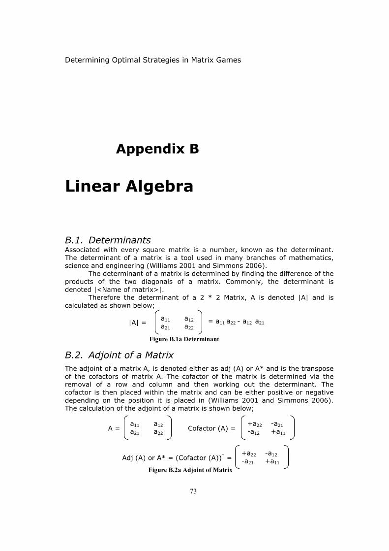
Determining Optimal Strategies in Matrix Games
73
Appendix B
Linear Algebra
B.1. Determinants Associated with every square matrix is a number, known as the determinant.
The determinant of a matrix is a tool used in many branches of mathematics, science and engineering (Williams 2001 and Simmons 2006). The determinant of a matrix is determined by finding the difference of the products of the two diagonals of a matrix. Commonly, the determinant is
denoted |<Name of matrix>|. Therefore the determinant of a 2 * 2 Matrix, A is denoted |A| and is calculated as shown below;
B.2. Adjoint of a Matrix
The adjoint of a matrix A, is denoted either as adj (A) or A* and is the transpose of the cofactors of matrix A. The cofactor of the matrix is determined via the removal of a row and column and then working out the determinant. The cofactor is then placed within the matrix and can be either positive or negative
depending on the position it is placed in (Williams 2001 and Simmons 2006). The calculation of the adjoint of a matrix is shown below; a11 a12
a21 a22
A =
+a22 -a21 -a12 +a11
Cofactor (A) =
+a22 -a12 -a21 +a11
Adj (A) or A* = (Cofactor (A))T =
Figure B.2a Adjoint of Matrix
a11 a12 a21 a22
= a11 a22 - a12 a21
Figure B.1a Determinant
|A| =

Determining Optimal Strategies in Matrix Games
74
B.3. Multiplication of Vectors and Matrices
The multiplication of vectors and matrices is determined via the sum of products of the corresponding rows of a matrix with the columns of the vector. The figure below shows the multiplication of vectors and matrices.
B.4. Multiplication of Elements and Matrices The multiplication of elements and matrices is referred to as a Scalar Multiple (Williams 2001). Scalar multiple of a matrix is determined by multiplying every
single element inside the matrix with the scalar value (Williams 2001). The resulting scalar matrix will be the same size as the original matrix. The figure below shows scalar multiplication of a matrix;
B.5. Multiplication of Two Vectors The multiplication of two vectors is referred to as the Dot Product (Williams
2001). The dot product is calculated via the sum of products of the corresponding elements within the two vectors (Williams 2001 and Simmons 2006), as shown below;
U = (x1, y1) V = (x2, y2) Dot product of U and V denoted as U.V = x1x2 + y1y2 Figure B.5a Dot Product of Two Vectors
Xa11 Xa12 Xa21 Xa22
XA =
Figure B.4a Scalar Multiplication of Matrix
Scalar Value = X
a11 a12 a21 a22
A =
AV = [xa11 + xa21, ya12 + ya22] Figure B.3a Multiplication of Vectors and Matrix
V = [x, y]
a11 a12 a21 a22
A =

Determining Optimal Strategies in Matrix Games
75
Appendix C
Source Code
This Appendix contains the source for the 2*2 Matrix and 2*N Matrix Classes.

Determining Optimal Strategies in Matrix Games
76

Determining Optimal Strategies in Matrix Games
77

Determining Optimal Strategies in Matrix Games
78

Determining Optimal Strategies in Matrix Games
79

Determining Optimal Strategies in Matrix Games
80

Determining Optimal Strategies in Matrix Games
81

Determining Optimal Strategies in Matrix Games
82

Determining Optimal Strategies in Matrix Games
83

Determining Optimal Strategies in Matrix Games
84

Determining Optimal Strategies in Matrix Games
85

Determining Optimal Strategies in Matrix Games
86

Determining Optimal Strategies in Matrix Games
87
Appendix D
Test Cases
This appendix contains the test scripts for the unit testing and system testing of the 2*2 Matrix Class and 2*N Matrix Class.
The test cases give an indication of whether the test passed or failed and allowed the tester to add further comments.

Determining Optimal Strategies in Matrix Games
88
D.1 Two by Two Matrix Game Test Scripts All of the following test scripts were performed using the following conditions;
Laptop Type – Sony VAIO PCG-FR285M Application Version – Two By Two Matrix Operating System – Microsoft Windows XP Home Edition Version 2002 Service Pack 2
Processor – Pentium (R) 4 CPU 2.40 GHz Memory – 488 MB of RAM IDE – Eclipse SDK Version 3.2.2
Unit Test Case 1: Creation a random matrix and printing the random matrix
BRIEF DESCRIPTION:
This test case will test the following requirements; � 3.3.1.1 – Matrix generated by the program must be of correct size � 3.3.1.3 – The application must provide the means, for elements to be randomly generated inside the matrix
� 3.3.1.5 – Elements in the matrix table must be valid i.e. not characters, floats and string
PREPARATION:
Run the Two by Two Matrix code on Eclipse. When program starts enter in your name.
ACTION: EXPECTED RESULT:
ACTUAL
RESULT
(PASS/FAIL)
COMMENTS
1. The program should welcome the user, to the
application. The program will ask the user to either chose 1 to generate a random matrix or 2
to generate a matrix, in which users can enter in data themselves.
1. The user should be given a choice of 1 to
generate a random matrix or 2 to generate a matrix, in which users can enter in data
themselves. 2. The program should state that the number
PASS
Possible extension to the program is that when illegal parameters are
entered, such as strings etc… that

Determining Optimal Strategies in Matrix Games
89
2. Enter in the number 3. 3. Enter in number -1.
4. Enter in a character. 5. Re-do preparation and enter in a string. 6. Re-do preparation and enter in a float.
7. Re-do preparation and enter in 1.
three is not a valid choice and will ask the user to enter in valid data, such as 0 or 1.
3. See expected result number 2. 4. Program should terminate indicating to the
user that an illegal data type was entered.
5. See expected result number 4. 6. See expected result number 4. 7. This is valid data. Program should generate a
two dimensional matrix with the column and
row size of 2. The elements inside the matrix should be randomly generated. The application should print off the matrix.
the program should not
terminate but should loop, until valid parameters
are entered.
Unit Test Case 2: Creation of user specified matrix and printing the user specified matrix
BRIEF DESCRIPTION:
This test case will test the following requirements;
� 3.3.1.1 – Matrix generated by the program must be of correct size � 3.3.1.4 – The application must provide the means, for elements to be entered inside the matrix, by users � 3.3.1.5 – Elements in the matrix table must be valid i.e. not characters, floats and string
PREPARATION:
Run the Two by Two Matrix code on Eclipse. When program starts enter in your name.
ACTION: EXPECTED RESULT:
ACTUAL
RESULT
(PASS/FAIL)
COMMENTS
1. The program should welcome the user, to the
application. The program will ask the user to either chose 1 to generate a random matrix or 2
1. The user should be given a choice of 1 to
generate a random matrix or 2 to generate a matrix, in which users can enter in data
PASS
Possible extension to the program is
that when illegal parameters are
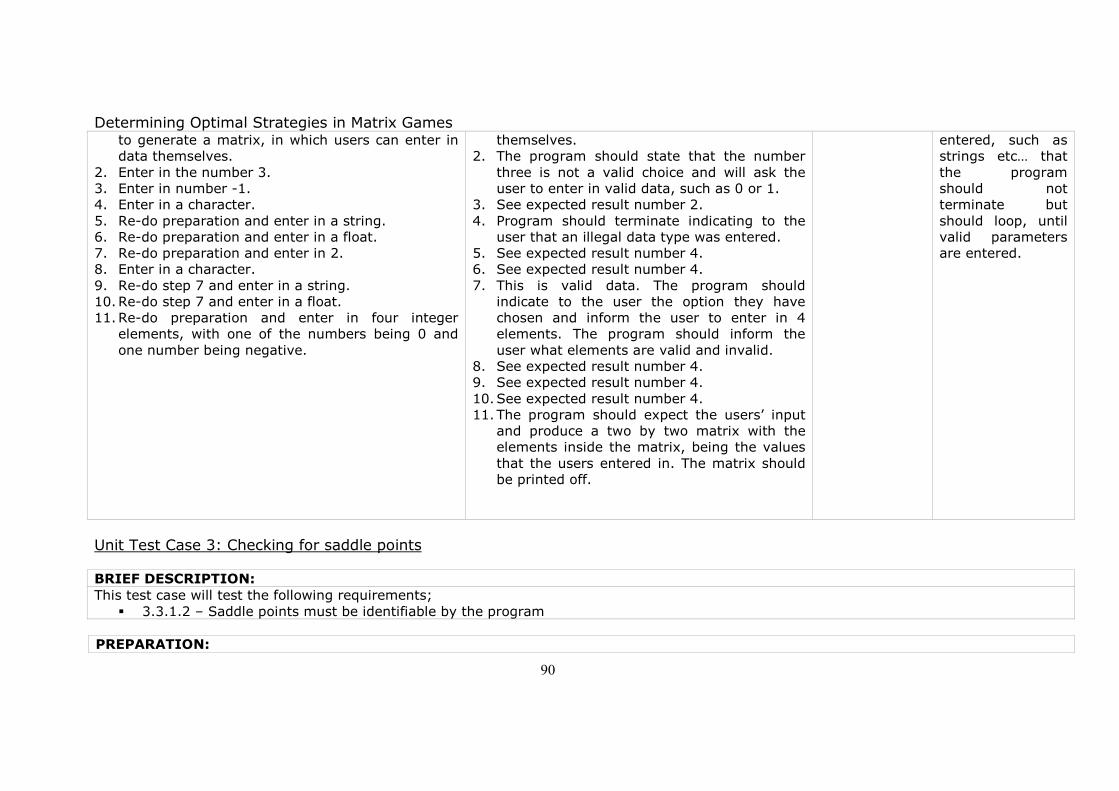
Determining Optimal Strategies in Matrix Games
90
to generate a matrix, in which users can enter in data themselves.
2. Enter in the number 3. 3. Enter in number -1. 4. Enter in a character.
5. Re-do preparation and enter in a string. 6. Re-do preparation and enter in a float. 7. Re-do preparation and enter in 2. 8. Enter in a character.
9. Re-do step 7 and enter in a string. 10. Re-do step 7 and enter in a float. 11. Re-do preparation and enter in four integer
elements, with one of the numbers being 0 and
one number being negative.
themselves. 2. The program should state that the number
three is not a valid choice and will ask the user to enter in valid data, such as 0 or 1.
3. See expected result number 2.
4. Program should terminate indicating to the user that an illegal data type was entered.
5. See expected result number 4. 6. See expected result number 4.
7. This is valid data. The program should indicate to the user the option they have chosen and inform the user to enter in 4 elements. The program should inform the
user what elements are valid and invalid. 8. See expected result number 4. 9. See expected result number 4.
10. See expected result number 4. 11. The program should expect the users’ input
and produce a two by two matrix with the elements inside the matrix, being the values
that the users entered in. The matrix should be printed off.
entered, such as strings etc… that
the program should not terminate but
should loop, until valid parameters are entered.
Unit Test Case 3: Checking for saddle points
BRIEF DESCRIPTION:
This test case will test the following requirements;
� 3.3.1.2 – Saddle points must be identifiable by the program
PREPARATION:

Determining Optimal Strategies in Matrix Games
91
Generate the following user specified matrices {{1, 0}, {-1, 2}} and {{-2, -2}, {3, 0}} and two randomly generated matrices and assign them to different two dimensional matrices.
ACTION: EXPECTED RESULT:
ACTUAL
RESULT
(PASS/FAIL)
COMMENTS
1. Run the function saddle point, passing the first
user specified matrix. 2. Run the function saddle point, passing the second
user specified matrix. 3. Run the function saddle point, passing the first
randomly generated matrix. 4. Run the function saddle point, passing the second
randomly generated matrix.
1. The program should state to the user that the
matrix does not have any saddle points. 2. The program should state to the user that the
element 0, in matrix position 2, 2 is the saddle point.
3. Depending on the matrix generated, the program should either state that there is a saddle point and state the element. Or the
program should state that no saddle point exists within the matrix.
4. See expected result 3.
PASS
Unit Test Case 4: Calculating the determinant
BRIEF DESCRIPTION:
This test case will test the following requirements; � 3.3.1.7.1 – The determinant of the matrix must be calculated.
� 3.3.1.9.3 – Calculate the numerator for the following formula |A| /JA*JT.
PREPARATION:
Re-use the matrices without saddle points used in unit test 3. The random matrix without saddle points that were used in unit test 3 was; {{93, 4}, {7, 55}}
The user specified matrix without saddle points that were used in unit test 3 was; {{1, 0}, {-1, 2}}

Determining Optimal Strategies in Matrix Games
92
ACTION: EXPECTED RESULT:
ACTUAL
RESULT
(PASS/FAIL)
COMMENTS
1. Run the function determinant passing the random
matrix specified in the preparation. 2. Run the function determinant this time passing
the user specified matrix specified in the preparation.
1. The program should calculate the
determinant8. 2. The program should calculate the
determinant9.
PASS
Unit Test Case 5: Performing the adjoint operation on a matrix and printing off the adjoint matrix
BRIEF DESCRIPTION:
This test case will test the following requirements; � 3.3.1.7.2 – The adjoint of the matrix must be calculated.
PREPARATION:
Re-use matrices that were used in unit test 4.
ACTION: EXPECTED RESULT:
ACTUAL
RESULT
(PASS/FAIL)
COMMENTS
1. Run the function adjoint passing the random
matrix specified in the preparation.
2. Run the function adjoint passing the user specified matrix specified in the preparation.
1. The program should produce the adjoint of
the random matrix10.
2. The program should produce the adjoint of the user specified matrix11.
PASS
8 See Appendix E – Test Data, for manual results. 9 See Appendix E – Test Data, for manual results.

Determining Optimal Strategies in Matrix Games
93
Unit Test Case 6: Calculating the numerator for the formula (4.3.2.2.1)
BRIEF DESCRIPTION:
This test case will test the following requirements; � 3.3.1.9.1 – Calculate probability for player one by calculating the numerator for the following formula JA*/JA*JT.
PREPARATION:
Re-use matrices that were used in unit test 5.
ACTION: EXPECTED RESULT:
ACTUAL
RESULT
(PASS/FAIL)
COMMENTS
1. Run the function vector times adjoint passing the random matrix specified in the preparation.
2. Run the function vector times adjoint passing the
user specified matrix specified in the preparation.
1. The program should calculate using the random matrix, the JA* which is the numerator used in the formula (4.3.2.2.1) 12.
2. The program should calculate using the user specified matrix, the JA* which is the numerator used in the formula (4.3.2.2.1) 13.
PASS
Unit Test Case 7: Calculating the denominator for the formulas (4.3.2.2.1), (4.3.2.2.2) and (4.3.2.2.3)
BRIEF DESCRIPTION:
This test case will test the following requirements; � 3.3.1.9 – Calculate the denominator for the following formula JA*/JA*JT.
� 3.3.1.9 – Calculate the denominator for the following formula A*JT /JA*JT.
10 See Appendix E – Test Data, for manual results. 11 See Appendix E – Test Data, for manual results. 12 See Appendix E – Test Data, for manual results. 13 See Appendix E – Test Data, for manual results.

Determining Optimal Strategies in Matrix Games
94
� 3.3.1.9 – Calculate the denominator for the following formula |A|/JA*JT.
PREPARATION:
Re-use matrices that were used in unit test 6.
ACTION: EXPECTED RESULT:
ACTUAL
RESULT
(PASS/FAIL)
COMMENTS
1. Run the function vector times adjoint times vector
times transpose, passing the random matrix as specified in the preparation.
2. Run the function vector times adjoint times vector
times transpose, passing the user specified matrix as specified in the preparation.
1. The program should calculate using the
random matrix, the JA*JT which is the denominator used in formulas; (4.3.2.2.1), (4.3.2.2.2) and (4.3.2.2.3) 14.
2. The program should calculate using the user specified matrix, the JA*JT which is the denominator used in the formulas (4.3.2.2.1), (4.3.2.2.2) and (4.3.2.2.3) 15.
PASS
Unit Test Case 8: Calculating the numerator for the formula (4.3.2.2.2)
BRIEF DESCRIPTION:
This test case will test the following requirements;
� 3.3.1.9.2 – Calculate the numerator for the following formula A*JT /JA*JT.
PREPARATION:
Re-use matrices that were used in unit test 7.
14 See Appendix E – Test Data, for manual results. 15 See Appendix E – Test Data, for manual results.

Determining Optimal Strategies in Matrix Games
95
ACTION: EXPECTED RESULT:
ACTUAL
RESULT
(PASS/FAIL)
COMMENTS
1. Run the function adjoint times vector times transpose, passing the random matrix as specified in the preparation.
2. Run the function adjoint times vector times
transpose, passing the user specified matrix as specified in the preparation.
1. The program should calculate using the random matrix, the A*JT which is the numerator used in the formula (4.3.2.2.2)16.
2. The program should calculate using the user
specified matrix, the A*JT which is the numerator used in the formula (4.3.2.2.2) 17.
PASS
Unit Test Case 9: Calculating the numerator for the formula (4.3.2.2.3)
BRIEF DESCRIPTION:
This test case will test the following requirements; � 3.3.1.9.3 – Calculate the numerator for the following formula |A| /JA*JT.
PREPARATION:
Re-use matrices that were used in unit test 8.
ACTION: EXPECTED RESULT:
ACTUAL
RESULT
(PASS/FAIL)
COMMENTS
1. See unit test 4.
1. See unit test 4.
PASS
16 See Appendix E – Test Data, for manual results. 17 See Appendix E – Test Data, for manual results.

Determining Optimal Strategies in Matrix Games
96
Unit Test Case 10: Calculating the probability for players I and II
BRIEF DESCRIPTION:
This test case will test the following requirements; � 3.3.1.8 – Using the determinant, J vector, transpose of J vector and original matrix values, the program must be able to work out, the
probabilities for the players involved in the game and the payoff of the game
PREPARATION:
Use 2*2 matrices specified in Appendix <appendix name � testing and test data handout>
ACTION: EXPECTED RESULT:
ACTUAL
RESULT
(PASS/FAIL)
COMMENTS
1. Run the function prob payoff, using the results
gathered from the random matrix.
2. Run the function prob payoff, using the results gathered from the user specified matrix.
1. The program should calculate the probability
for both players18.
2. The program should calculate the probability for both players19.
PASS
Unit Test Case 11: Performing probability validity check
BRIEF DESCRIPTION:
This test case will test the following requirements; � 3.3.1.10 – The program must indicate whether the probabilities are valid or invalid.
PREPARATION:
Re-use the probabilities gathered from unit test 10.
18 See Appendix E – Test Data, for manual results. 19 See Appendix E – Test Data, for manual results.

Determining Optimal Strategies in Matrix Games
97
ACTION: EXPECTED RESULT:
ACTUAL
RESULT
(PASS/FAIL)
COMMENTS
1. Pass the probabilities from the random matrix into the function check.
2. Pass the probabilities from the user specified matrix into the function check.
3. Pass the values (1, 3) into the function check. 4. Pass the values (1/4, 3/4) into the function check. 5. Pass the values (-1, 2) into the function check.
6. Pass values (-2/5, 3/5) into the function check.
1. The program should determine that the probabilities are valid20.
2. The program should determine that the probabilities are valid21.
3. The program should state that the probabilities are invalid.
4. The program should state that the
probabilities are valid. 5. The program should state that the
probabilities are invalid. 6. The program should state that the
probabilities are invalid.
PASS
Unit Test Case 12: Calculating the payoff
BRIEF DESCRIPTION:
This test case will test the following requirements; � 3.3.1.8 – Using the determinant, adjoint, transpose and original matrix values, the program must be able to work out the payoff for the
players involved in the game.
PREPARATION:
Re-use values that were used in unit test 10.
20 See Appendix E – Test Data, for manual results. 21 See Appendix E – Test Data, for manual results.

Determining Optimal Strategies in Matrix Games
98
ACTION: EXPECTED RESULT:
ACTUAL
RESULT
(PASS/FAIL)
COMMENTS
1. Run the function prob payoff, using the results
gathered from the random matrix. 2. Run the function prob payoff, using the results
gathered from the user specified matrix.
1. The program should calculate the payoff of
the game22. 2. The program should calculate the payoff of
the game23.
PASS
System Test Case 1: System Test
BRIEF DESCRIPTION:
This test case will test all of the requirements specified in Section 3.3.1 and the specification mentioned in Section 4.3.2.
PREPARATION:
Have the original main method of the application executed. Use user specified matrices that were used in the unit tests.
ACTION: EXPECTED RESULT:
ACTUAL
RESULT
(PASS/FAIL)
COMMENTS
1. Enter your name. 2. Enter in 1.
3. Run the application again. 4. Enter your name.
1. Program should greet the user with a
welcome message.
2. Random matrix should be generated and optimal strategies and payoff should be
PASS
22 See Appendix E – Test Data, for manual results. 23 See Appendix E – Test Data, for manual results.

Determining Optimal Strategies in Matrix Games
99
5. Enter in 2. 6. Enter in the user specified matrix that had saddle
point. 7. Re-do steps 3 – 5. 8. Enter in the user specified matrix that had no
saddle points.
determined. 3. Program should ask for the users’ name.
4. Program should greet the user with a welcome message and ask the user whether they wish to randomly generate a matrix or
enter in the elements into a blank 2*2 matrix, themselves.
5. Program should ask the user to enter in four integer values.
6. The program should state that the matrix does have a saddle point.
7. See expected results 3 – 5. 8. The program should state that the matrix
does not have a saddle point and therefore workout the probabilities and payoff of the players, using the formulas and then
checking to see if the probabilities are valid or not.

Determining Optimal Strategies in Matrix Games
100
D.2 Two by N Matrix Game Test Scripts All of the following test scripts were performed using the following conditions;
Laptop Type – Sony VAIO PCG-FR285M Application Version – Two By N Matrix Operating System – Microsoft Windows XP Home Edition Version 2002 Service Pack 2
Processor – Pentium (R) 4 CPU 2.40 GHz Memory – 488 MB of RAM IDE – Eclipse SDK Version 3.2.2
Unit Test Case 1: Creation of the 2*N matrix
BRIEF DESCRIPTION:
This test case will test the following requirement; � 3.3.2.1 – Program must allow users to enter in the length or width of their choice or randomly generate the length or width of the
matrices.
PREPARATION:
Run the Two by N Matrix code on Eclipse.
ACTION: EXPECTED RESULT:
ACTUAL
RESULT
(PASS/FAIL)
COMMENTS
1. Enter in string. 2. Rerun the code again. 3. Enter in a float. 4. Rerun the code again.
5. Enter in a negative number. 6. Enter in the number 0.
1. Program should inform the user that invalid data was entered and then terminate.
2. Program should ask the user to enter in the number of columns they wish the matrix to
have. 3. See expected result 1.
PASS
Possible extension
to the program is that when illegal parameters are entered, such as
strings etc… that the program
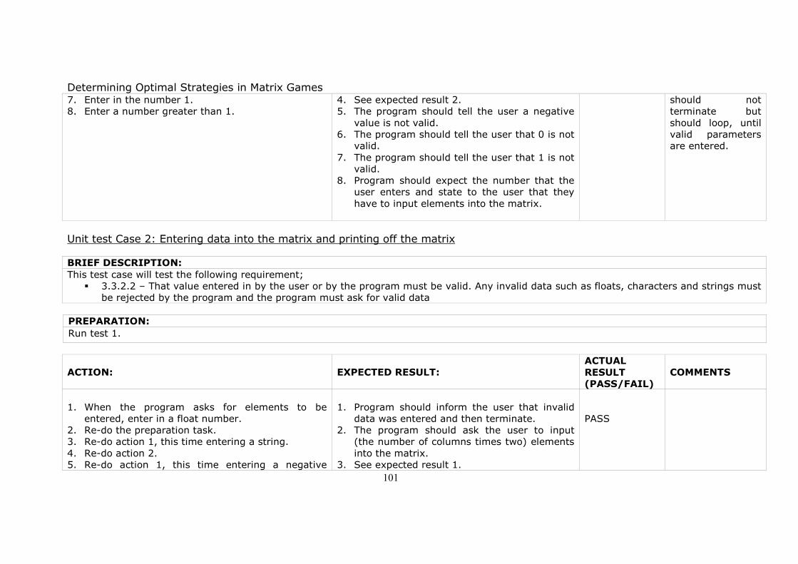
Determining Optimal Strategies in Matrix Games
101
7. Enter in the number 1. 8. Enter a number greater than 1.
4. See expected result 2. 5. The program should tell the user a negative
value is not valid. 6. The program should tell the user that 0 is not
valid.
7. The program should tell the user that 1 is not valid.
8. Program should expect the number that the user enters and state to the user that they
have to input elements into the matrix.
should not terminate but
should loop, until valid parameters are entered.
Unit test Case 2: Entering data into the matrix and printing off the matrix
BRIEF DESCRIPTION:
This test case will test the following requirement; � 3.3.2.2 – That value entered in by the user or by the program must be valid. Any invalid data such as floats, characters and strings must
be rejected by the program and the program must ask for valid data
PREPARATION:
Run test 1.
ACTION: EXPECTED RESULT:
ACTUAL
RESULT
(PASS/FAIL)
COMMENTS
1. When the program asks for elements to be entered, enter in a float number.
2. Re-do the preparation task. 3. Re-do action 1, this time entering a string.
4. Re-do action 2. 5. Re-do action 1, this time entering a negative
1. Program should inform the user that invalid data was entered and then terminate.
2. The program should ask the user to input (the number of columns times two) elements
into the matrix. 3. See expected result 1.
PASS

Determining Optimal Strategies in Matrix Games
102
integer. 6. Enter a positive integer.
7. Enter the integer 0. 8. Enter more integer elements until the matrix is
full.
4. See expected result 2. 5. Program should expect the negative integer
and inform the user that there are (number of columns - 1) elements left to enter into the matrix.
6. Program should expect the positive integer and inform the user of the number of elements left to enter into the matrix.
7. Program should expect the integer 0 and
inform the user of the number of elements left to enter into the matrix.
8. User should be able to enter the elements into the matrix. Once the matrix is full, the
program should print off the matrix.
Unit Test Case 3: Working out the linear equations of the lines
BRIEF DESCRIPTION:
This test case will verify that the program, produces linear equations from 2*N matrices. The equations will be used to determine optimal strategies and payoffs for the players.
PREPARATION:
Create a 2*4 matrix and input the following elements into the matrix; {{2, 3, 1, 5},{4, 1, 6, 0}}
ACTION: EXPECTED RESULT:
ACTUAL
RESULT
(PASS/FAIL)
COMMENTS
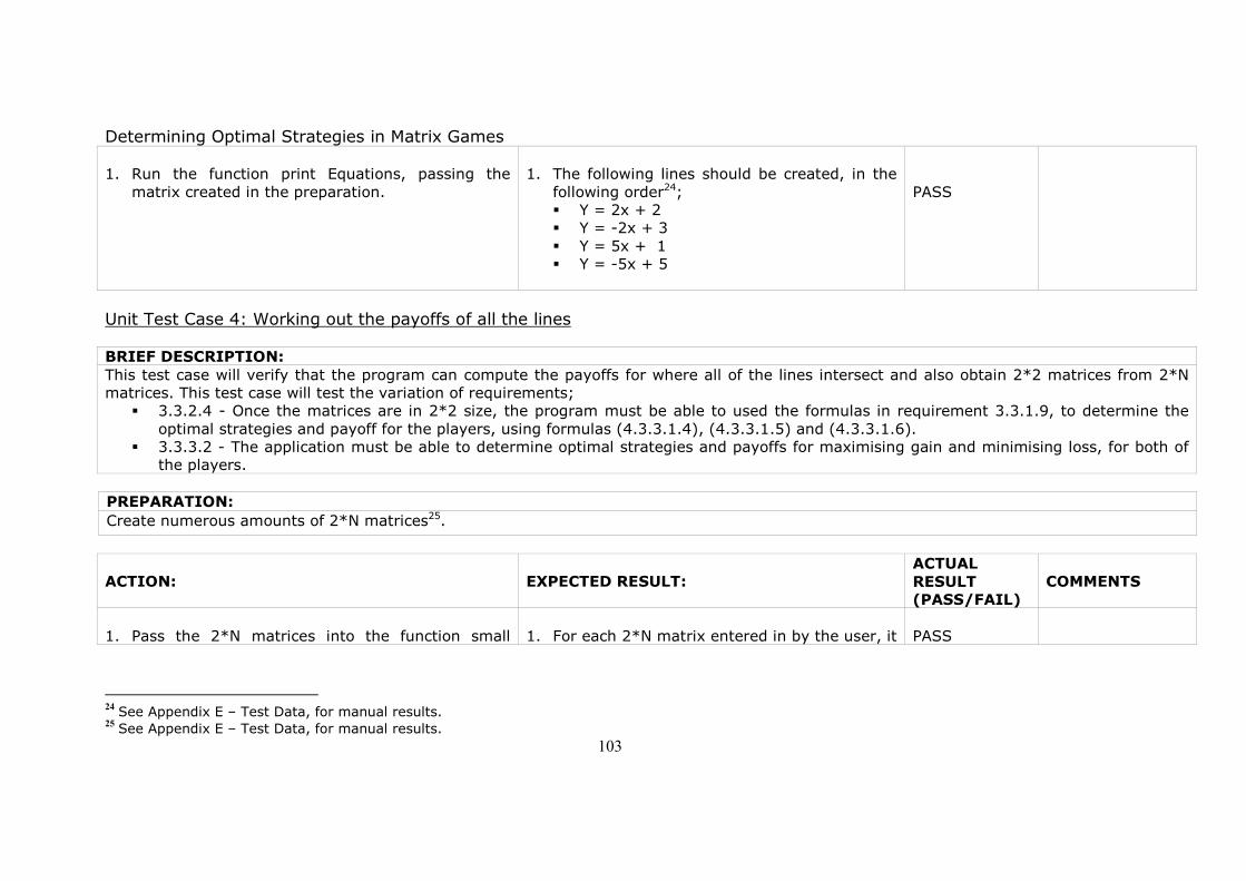
Determining Optimal Strategies in Matrix Games
103
1. Run the function print Equations, passing the
matrix created in the preparation.
1. The following lines should be created, in the
following order24; � Y = 2x + 2 � Y = -2x + 3
� Y = 5x + 1 � Y = -5x + 5
PASS
Unit Test Case 4: Working out the payoffs of all the lines
BRIEF DESCRIPTION:
This test case will verify that the program can compute the payoffs for where all of the lines intersect and also obtain 2*2 matrices from 2*N matrices. This test case will test the variation of requirements;
� 3.3.2.4 - Once the matrices are in 2*2 size, the program must be able to used the formulas in requirement 3.3.1.9, to determine the
optimal strategies and payoff for the players, using formulas (4.3.3.1.4), (4.3.3.1.5) and (4.3.3.1.6). � 3.3.3.2 - The application must be able to determine optimal strategies and payoffs for maximising gain and minimising loss, for both of
the players.
PREPARATION:
Create numerous amounts of 2*N matrices25.
ACTION: EXPECTED RESULT:
ACTUAL
RESULT
(PASS/FAIL)
COMMENTS
1. Pass the 2*N matrices into the function small
1. For each 2*N matrix entered in by the user, it
PASS
24 See Appendix E – Test Data, for manual results.
25 See Appendix E – Test Data, for manual results.

Determining Optimal Strategies in Matrix Games
104
matrix and into the function small matrix payoff. will be displayed as a combination of 2*2 matrixes and for each 2*2 matrix, the payoff
should be computed26.
Unit Test Case 5: Working out the probabilities of all the lines
BRIEF DESCRIPTION:
This test case will verify that the program can compute the probabilities for where all of the lines intersect. This test case will test the variation of requirements;
� 3.3.2.4 - Once the matrices are in 2*2 size, the program must be able to used the formulas in requirement 3.3.1.9, to determine the
optimal strategies and payoff for the players, using formulas (4.3.3.1.4), (4.3.3.1.5) and (4.3.3.1.6). � 3.3.3.2 - The application must be able to determine optimal strategies and payoffs for maximising gain and minimising loss, for both of
the players.
PREPARATION:
Re-use matrices from unit test 4.
ACTION: EXPECTED RESULT:
ACTUAL
RESULT
(PASS/FAIL)
COMMENTS
1. Pass the 2*N matrix into the function small matrix
player 1 and small matrix player 2.
1. For each 2*N matrix entered in by the user, it
will be displayed as a combination of 2*2 matrices and for each 2*2 matrix, the probabilities for the intersecting lines should
be computed27.
PASS
26 See Appendix E – Test Data, for manual results.
27 See Appendix E – Test Data, for manual results.

Determining Optimal Strategies in Matrix Games
105
Unit Test Case 6: Performing probability validity check
BRIEF DESCRIPTION:
This test case will check to see that the following requirement; � 3.3.1.10 should be maintained for 2*N matrices.
PREPARATION:
Reuse the probabilities determined in unit test 5. Alter the code for the function check, by adding print statements, indicating whether the if statement is true or false.
ACTION: EXPECTED RESULT:
ACTUAL
RESULT
(PASS/FAIL)
COMMENTS
1. Pass the values (1.0, 0.0) into the check function. 2. Pass the values (-1.0, 2.0) into the check
function. 3. Pass the values (-0.25, 1.25) into the check
function.
4. Pass the values (0.2, 0.8) into the check function. 5. Pass the values (0.3, 0.65) into the check
function.
1. The program should state that the
probabilities are valid.
2. The program should state that the probabilities are invalid.
3. The program should state that the
probabilities are invalid. 4. The program should state that the
probabilities are valid. 5. The program should state that the
probabilities are invalid.
PASS
Unit Test Case 7: Determining the case of the graphical nature of the matrix
BRIEF DESCRIPTION:
This test case will verify that the program can determine the cases of matrices entered in by the user. This test case will test the variation of requirements;

Determining Optimal Strategies in Matrix Games
106
� 3.3.3.1 - The matrix must be able to be represented in a graph.
PREPARATION:
Use the matrices specified in Appendix E.
ACTION: EXPECTED RESULT:
ACTUAL
RESULT
(PASS/FAIL)
COMMENTS
1. Run the application, with each of the matrices.
1. For each matrix, the graphical nature should
be identified.
PASS

Determining Optimal Strategies in Matrix Games
107
System Test Case 1: System Test
BRIEF DESCRIPTION:
This test case will test the majority of the requirements specified in Section 3.3.2 and 3.3.3 and all of the specification mentioned in Section 4.3.3.
PREPARATION:
Have Appendix E to hand.
ACTION: EXPECTED RESULT:
ACTUAL
RESULT
(PASS/FAIL)
COMMENTS
1. Run the main function passing the matrices from Section E.2 of Appendix E – Test Data.
1. The optimal strategies and payoff that the application generates, should match the optimal strategies and payoff worked out in
Section E.2 of Appendix E – Test Data.
FAIL
There is a crash with case 1 for the 2*5 matrix – this
is due to 3 lines intersecting at on point. Algorithm for case
2 has got a flaw in it.

Determining Optimal Strategies in Matrix Games
108
Appendix E
Test Data
This Appendix contains the test data for the 2*2 and 2*N Matrix Classes, that was used with Appendix D, during the testing of the applications. The appendix
is structured starting with the 2*2 matrices and then 2*N matrices. The 2*N section is further structured by showing the diagrams of each 2*N matrix, used in the testing and then manually working out the solution for
each matrix.

Determining Optimal Strategies in Matrix Games
109
E.1. 2*2 Test Data
Saddle points A saddle point is an element aij in the matrix, where it is both the maximum entry in its column and the minimum entry in its row.
Formula
x = JA*/JA*JT y = A*JT / JA*JT v = |A|/ JA*JT
a11 a12 a21 a22
= a11 a22 - a12 a21
|A| =
a11 a12 a21 a22
A =
+a22 -a21 -a12 +a11
Cofactor (A) =
+a22 -a12 -a21 +a11
Adj (A) or A* = (Cofactor (A))T =
Xa11 Xa12 Xa21 Xa22
XA =
Scalar Value = X
a11 a12 a21 a22
A =
U = (x1, y1) V = (x2, y2) Dot product of U and V denoted as U.V = x1x2 + y1y2
AV = [xa11 + xa21, ya12 + ya22]
V = [x, y]
a11 a12 a21 a22
A =

Determining Optimal Strategies in Matrix Games
110
E.1.1 User Generated Matrices
No Saddle point
Need to use the formula to work out unique optimal strategies for Players I and II and their corresponding payoff.
|A| = (1)2 – 0(-1) = 2 – 0 = 2
J = (1, 1)
Player I = (¾, ¼) Player II = (½, ½) Payoff, v = ½
Probabilities for Player I and Player II are both valid.
1 0
-1 2 Matrix 1 =
+2 -0
--1 +1 A* = 2 0
1 1 =
-2 -2
3 0 Matrix 2 =
JT = 1 1
A*JT = 2 0
1 1 1 1
2(1) + 0(1) 1(1) + 1(1)
= 2+0 1+1
2 2 = =
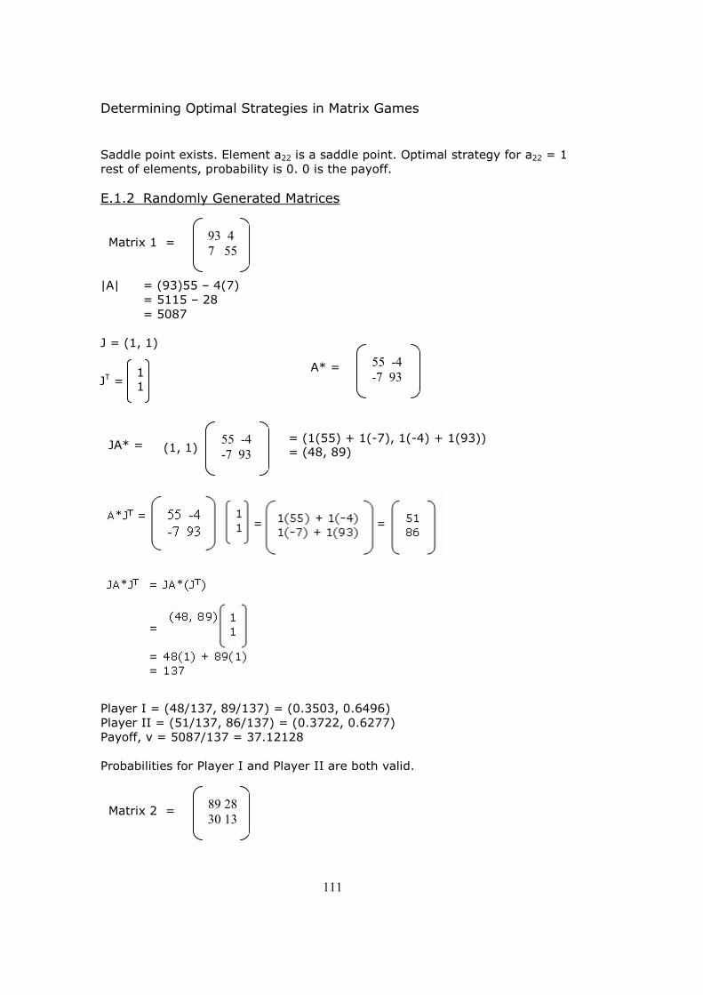
Determining Optimal Strategies in Matrix Games
111
Saddle point exists. Element a22 is a saddle point. Optimal strategy for a22 = 1 rest of elements, probability is 0. 0 is the payoff.
E.1.2 Randomly Generated Matrices
|A| = (93)55 – 4(7) = 5115 – 28
= 5087 J = (1, 1)
Player I = (48/137, 89/137) = (0.3503, 0.6496) Player II = (51/137, 86/137) = (0.3722, 0.6277) Payoff, v = 5087/137 = 37.12128
Probabilities for Player I and Player II are both valid.
93 4
7 55 Matrix 1 =
55 -4
-7 93 A* =
89 28
30 13 Matrix 2 =
JT = 1 1
JA* = (1, 1) = (1(55) + 1(-7), 1(-4) + 1(93)) = (48, 89)
55 -4
-7 93

Determining Optimal Strategies in Matrix Games
112
Saddle point exists. Element a12 is a saddle point. Optimal strategy for a12 = 1 rest of elements, probability is 0. 28 is the payoff.
E.2. 2*N Test Data Equation of lines
Y = (a2j – a1j) x + a1j
Probabilities of players and payoffs
Values used to work out whether the intersections determined from the matrices lye on a particular line;
((1-x), v)
x = a + d – b – c
d – c
y = a + d – b – c
d – b
v = a + d – b – c
ad – bc
Optimal strategies and payoffs in Matrix Games Player 1 = (x, 1-x)
Player 2 = (y, 1-y) Payoff = v
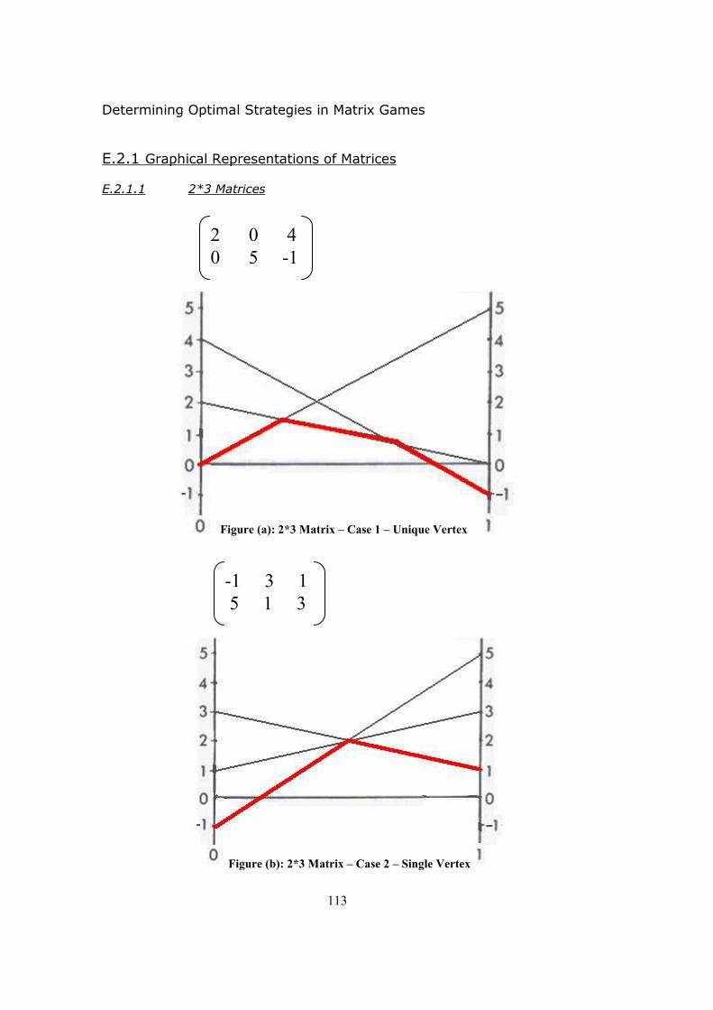
Determining Optimal Strategies in Matrix Games
113
E.2.1 Graphical Representations of Matrices
E.2.1.1 2*3 Matrices
2 0 4
0 5 -1
Figure (a): 2*3 Matrix – Case 1 – Unique Vertex
-1 3 1
5 1 3
Figure (b): 2*3 Matrix – Case 2 – Single Vertex

Determining Optimal Strategies in Matrix Games
114
E.2.1.2 2*4 Matrices
1 3 5
6 3 2
Figure (c): 2*3 Matrix – Case 3 – Two Vertices
2 3 1 5
4 1 6 0
Figure (a): 2*4 Matrix – Case 1 – Unique Vertex

Determining Optimal Strategies in Matrix Games
115
0 2 4 6
6 4 2 0
Figure (b): 2*4 Matrix – Case 2 – Single Vertex
1 2 4 5
4 2 2 0
Figure (c): 2*4 Matrix – Case 3 – Two Vertices
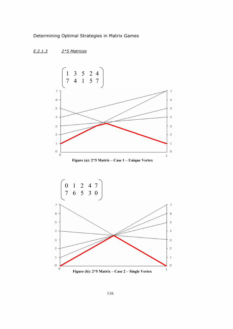
Determining Optimal Strategies in Matrix Games
116
E.2.1.3 2*5 Matrices
1 3 5 2 4
7 4 1 5 7
Figure (a): 2*5 Matrix – Case 1 – Unique Vertex
0 1 2 4 7
7 6 5 3 0
Figure (b): 2*5 Matrix – Case 2 – Single Vertex

Determining Optimal Strategies in Matrix Games
117
6 3 2 4 5
4 3 5 6 1
Figure (c): 2*5 Matrix – Case 3 – Two Vertices

Determining Optimal Strategies in Matrix Games
118
2 0 4
0 5 -1
2 0
0 5
X = (5-0) / (2+5-0-0) = 5/7 = 0.71428
Y = (5-0) / (2+5-0-0) = 5/7 = 0.71428
V = ((2*5) - (0*0)) / (2+5-0-0) = 10/7 = 1.42857
Player 1 = (5/7, 2/7) 2/7 = 0.28571
Player 2 = (5/7, 2/7)
V = 10/7
E.2.2 2*3 Matrices Test Data E.2.2.1 Case 1: One high vertex
Equation of lines:
Column Number Equation of Line
0 Y = -2x + 2
1 Y = 5x
2 Y = -5x + 4
2*3 Matrices � 2*2 Matrices
Number of matrices = 3
2 4
0 -1
X = (-1-0) / (2+ (-1)-4-0) = -1/-3 = 0.333333
Y = (-1-4) / (2+(-1)-4-0) = -5/-3 = 1.66666
V = ((2*(-1)) - (4*0)) / (2+(-1)-4-0) = -2/-3 = 0.66666
Player 1 = (1/3, 2/3) ±2/3 = ±0.66666
Player 2 = (5/3, -2/3)
V = 2/3
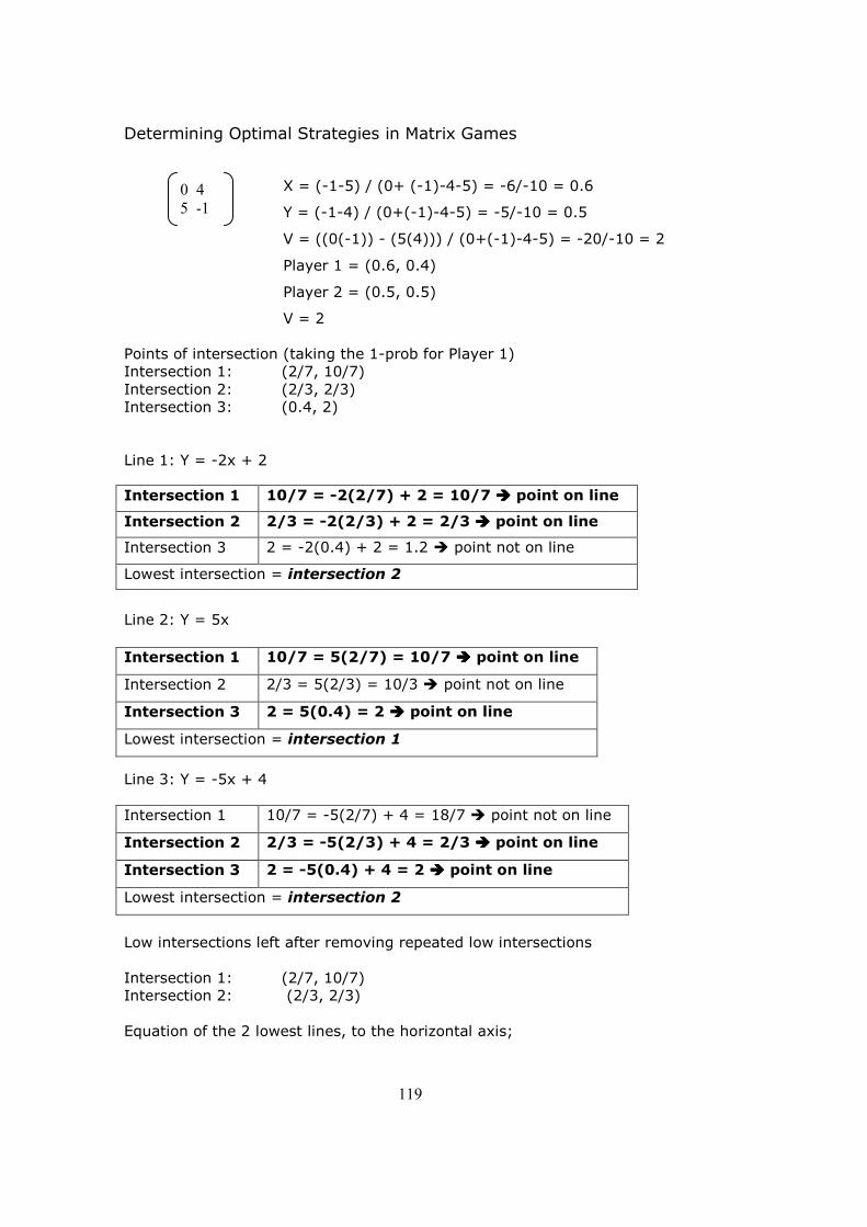
Determining Optimal Strategies in Matrix Games
119
Points of intersection (taking the 1-prob for Player 1) Intersection 1: (2/7, 10/7)
Intersection 2: (2/3, 2/3) Intersection 3: (0.4, 2)
Line 1: Y = -2x + 2
Line 2: Y = 5x
Line 3: Y = -5x + 4
Intersection 1 10/7 = -5(2/7) + 4 = 18/7 � point not on line
Intersection 2 2/3 = -5(2/3) + 4 = 2/3 ���� point on line
Intersection 3 2 = -5(0.4) + 4 = 2 ���� point on line
Lowest intersection = intersection 2
Low intersections left after removing repeated low intersections
Intersection 1: (2/7, 10/7) Intersection 2: (2/3, 2/3)
Equation of the 2 lowest lines, to the horizontal axis;
Intersection 1 10/7 = -2(2/7) + 2 = 10/7 ���� point on line
Intersection 2 2/3 = -2(2/3) + 2 = 2/3 ���� point on line
Intersection 3 2 = -2(0.4) + 2 = 1.2 � point not on line
Lowest intersection = intersection 2
Intersection 1 10/7 = 5(2/7) = 10/7 ���� point on line
Intersection 2 2/3 = 5(2/3) = 10/3 � point not on line
Intersection 3 2 = 5(0.4) = 2 ���� point on line
Lowest intersection = intersection 1
0 4
5 -1
X = (-1-5) / (0+ (-1)-4-5) = -6/-10 = 0.6
Y = (-1-4) / (0+(-1)-4-5) = -5/-10 = 0.5
V = ((0(-1)) - (5(4))) / (0+(-1)-4-5) = -20/-10 = 2
Player 1 = (0.6, 0.4)
Player 2 = (0.5, 0.5)
V = 2
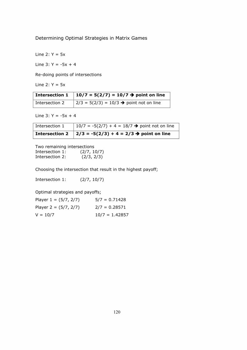
Determining Optimal Strategies in Matrix Games
120
Line 2: Y = 5x Line 3: Y = -5x + 4
Re-doing points of intersections Line 2: Y = 5x
Intersection 1 10/7 = 5(2/7) = 10/7 ���� point on line
Intersection 2 2/3 = 5(2/3) = 10/3 � point not on line
Line 3: Y = -5x + 4
Intersection 1 10/7 = -5(2/7) + 4 = 18/7 � point not on line
Intersection 2 2/3 = -5(2/3) + 4 = 2/3 ���� point on line
Two remaining intersections Intersection 1: (2/7, 10/7) Intersection 2: (2/3, 2/3)
Choosing the intersection that result in the highest payoff; Intersection 1: (2/7, 10/7)
Optimal strategies and payoffs;
Player 1 = (5/7, 2/7) 5/7 = 0.71428
Player 2 = (5/7, 2/7) 2/7 = 0.28571
V = 10/7 10/7 = 1.42857

Determining Optimal Strategies in Matrix Games
121
-1 3 1
5 1 3
E.2.2.2 Case 2: All intersections result in one unique vertex
2*3 Matrices � 2*2 Matrices
All intersecting points result in the same payoff. Optimal strategies and payoffs;
Player 1 = (0.5, 0.5)
Player 2 = (0.25, 0.75)
V = 2
-1 3
5 1
X = (1-5) / (-1+1-3-5) = -4/-8 = 0.5
Y = (1-3) / (-1+1-3-5) = -2/-8 = 0.25
V = ((-1(1)) - (3(5))) / (-1+1-3-5) = -16/-8 = 2
Player 1 = (0.5, 0.5)
Player 2 = (0.25, 0.75)
V = 2
-1 1
5 3
X = (3-5) / (-1+3-5-1) = -2/-4 = 0.5
Y = (3-1) / (-1+3-5-1) = 2/-4 = -0.5
V = ((-1(3)) - (1(5))) / (-1+3-5-1) = -8/-4 = 2
Player 1 = (1/2, 1/2)
Player 2 = (-1/2, 3/2)
V = 2
3 1
1 3
X = (3-1) / (3+3-1-1) = 2/4 = 0.5
Y = (3-1) / (3+3-1-1) = 2/4 = 0.5
V = ((3(3)) - (1(1))) / (3+3-1-1) = 8/4 = 2
Player 1 = (1/2, 1/2)
Player 2 = (1/2, 1/2)
V = 2

Determining Optimal Strategies in Matrix Games
122
1 3 5
6 3 2
E.2.2.3 Case 3: Two probabilities resulting in the same payoff
2*3 Matrices � 2*2 Matrices
Two intersecting points generate the same payoffs. Optimal strategies and payoffs between;
Player 1 = (1/3, 2/3) and (0.6, 0.4)
Player 2 = (1, 0) and (0, 1)
V = 3
1 5
6 2
X = (2-6) / (1+2-5-6) = -4/-8 = 0.5
Y = (2-5) / (1+2-5-6) = -3/-8 = 0.375
V = ((1(2)) - (5(6))) / (1+2-5-6) = -28/-8 = 3.5
Player 1 = (0.5, 0.5)
Player 2 = (0.375, 0.625)
V = 3.5
1 3
6 3
X = (3-6) / (1+3-3-6) = -3/-5 = 0.6
Y = (3-3) / (1+3-3-6) = 0/-5 = 0
V = ((1(3)) - (3(6))) / (1+3-3-6) = -15/-5 = 3
Player 1 = (0.6, 0.4)
Player 2 = (0, 1)
V = 3
3 5
3 2
X = (2-3) / (3+2-5-3) = -1/-3 = 1/3
Y = (2-5) / (3+2-5-3) = -3/-3 = 1
V = ((3(2)) - (5(3))) / (3+2-5-3) = -9/-3 = 3
Player 1 = (1/3, 2/3)
Player 2 = (1, 0)
V = 3

Determining Optimal Strategies in Matrix Games
123
2 3 1 5
4 1 6 0
E.2.3 2*4 Matrices Test Data E.2.3.1 Case 1 – one high vertex
Equation of lines:
Column Number Equation of Line
0 Y = 2x + 2
1 Y = -2x + 3
2 Y = 5x + 1
3 Y = -5x +5
2*4 Matrices � 2*2 Matrices
Number of matrices = 6
2 3
4 1
X = (1-4) / (2+1-3-4) = -3/-4 = 3/4
Y = (1-3) / (2+1-3-4) = -2/-4 = 1/2
V = ((2(1)) - (3(4))) / (2+1-3-4) = -10/-4 = 2.5
Player 1 = (3/4, 1/4)
Player 2 = (1/2, 1/2)
V = 2.5
2 1
4 6
X = (6-4) / (2+6-1-4) = 2/3
Y = (6-1) / (2+6-1-4) = 5/3
V = ((2(6)) - (1(4))) / (2+6-1-4) = 8/3
Player 1 = (2/3, 1/3)
Player 2 = (5/3, -2/3)
V = 8/3
2 5
4 0
X = (0-4) / (2+0-5-4) = -4/-7 = 4/7
Y = (0-5) / (2+0-5-4) = -5/-7 = 5/7
V = ((2(0)) - (5(4))) / (2+0-5-3) = -20/-7 = 20/7
Player 1 = (4/7, 3/7)
Player 2 = (5/7, 2/7)
V = 20/7
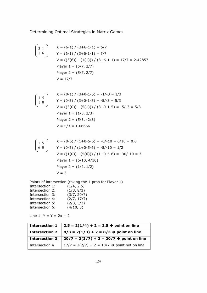
Determining Optimal Strategies in Matrix Games
124
Points of intersection (taking the 1-prob for Player 1) Intersection 1: (1/4, 2.5)
Intersection 2: (1/3, 8/3) Intersection 3: (3/7, 20/7) Intersection 4: (2/7, 17/7)
Intersection 5: (2/3, 5/3) Intersection 6: (4/10, 3) Line 1: Y = Y = 2x + 2
Intersection 1 2.5 = 2(1/4) + 2 = 2.5 ���� point on line
Intersection 2 8/3 = 2(1/3) + 2 = 8/3 ���� point on line
Intersection 3 20/7 = 2(3/7) + 2 = 20/7 ���� point on line
Intersection 4 17/7 = 2(2/7) + 2 = 18/7 � point not on line
3 1
1 6
3 5
1 0
1 5
6 0
X = (6-1) / (3+6-1-1) = 5/7
Y = (6-1) / (3+6-1-1) = 5/7
V = ((3(6)) - (1(1))) / (3+6-1-1) = 17/7 = 2.42857
Player 1 = (5/7, 2/7)
Player 2 = (5/7, 2/7)
V = 17/7
X = (0-1) / (3+0-1-5) = -1/-3 = 1/3
Y = (0-5) / (3+0-1-5) = -5/-3 = 5/3
V = ((3(0)) - (5(1))) / (3+0-1-5) = -5/-3 = 5/3
Player 1 = (1/3, 2/3)
Player 2 = (5/3, -2/3)
V = 5/3 = 1.66666
X = (0-6) / (1+0-5-6) = -6/-10 = 6/10 = 0.6
Y = (0-5) / (1+0-5-6) = -5/-10 = 1/2
V = ((1(0)) - (5(6))) / (1+0-5-6) = -30/-10 = 3
Player 1 = (6/10, 4/10)
Player 2 = (1/2, 1/2)
V = 3

Determining Optimal Strategies in Matrix Games
125
Line 2: Y = -2x + 3
Intersection 1 2.5 = -2(1/4) + 3 = 2.5 ���� point on line
Intersection 2 8/3 = -2(1/3) + 3 = 7/3 � point not on line
Intersection 3 20/7 = -2(3/7) + 3 = 15/7 � point not on line
Intersection 4 17/7 = -2(2/7) + 3 = 17/7 ���� point on line
Intersection 5 5/3 = -2(2/3) + 3 = 5/3 ���� point on line
Intersection 6 3 = -2(4/10) + 3 = 22/10 � point not on line
Lowest intersection = intersection 5
Line 3: Y = 5x + 1
Line 4: Y = -5x +5
Intersection 5 5/3 = 2(2/7) + 2 = 10/3 � point not on line
Intersection 6 3 = 2(4/10) + 2 = 28/10 � point not on line
Lowest intersection = intersection 1
Intersection 1 2.5 = 5(1/4) + 1 = 2.25 � point not on line
Intersection 2 8/3 = 5(1/3) + 1 = 8/3 ���� point on line
Intersection 3 20/7 = 5(3/7) + 1 = 22/7 � point not on line
Intersection 4 17/7 = 5(2/7) + 1 = 17/7 ���� point on line
Intersection 5 5/3 = 5(2/3) + 1 = 13/3 � point not on line
Intersection 6 3 = 5(4/10) + 1 = 3 ���� point on line
Lowest intersection = intersection 4
Intersection 1 2.5 = -5(1/4) +5 = 3.75 � point not on line
Intersection 2 8/3 = -5(1/3) +5 = 10/3 � point not on line
Intersection 3 20/7 = -5(3/7) +5 = 20/7 ���� point on line
Intersection 4 17/7 = -5(2/7) +5 = 25/7 � point not on line
Intersection 5 5/3 = -5(2/3) +5 = 5/3 ���� point on line
Intersection 6 3 = -5(4/10) +5 = 3 ���� point on line

Determining Optimal Strategies in Matrix Games
126
Removing repeated low intersections
Intersection 1: (1/4, 2.5) Intersection 4: (2/7, 17/7)
Intersection 5: (2/3, 5/3) Equation of the 2 lowest lines, to the horizontal axis Line 3: Y = 5x + 1
Line 4: Y = -5x +5
Re-doing points of intersections Line 3: Y = 5x + 1
Line 4: Y = -5x +5
Intersection 1 2.5 = -5(1/4) +5 = 3.75 � point not on line
Intersection 4 17/7 = -5(2/7) +5 = 25/7 � point not on line
Intersection 5 5/3 = -5(2/3) +5 = 5/3 ���� point on line
Two remaining intersections
Intersection 4: (2/7, 17/7) Intersection 5: (2/3, 5/3)
Choosing the intersection that result in the highest payoff;
Intersection 4: (2/7, 17/7)
Optimal strategies and payoffs;
Player 1 = (5/7, 2/7) 5/7 = 0.71428
Player 2 = (5/7, 2/7) 2/7 = 0.28571
V = 17/7 17/7 = 2.42857
Lowest intersection = intersection 5
Intersection 1 2.5 = 5(1/4) + 1 = 2.25 � point not on line
Intersection 4 17/7 = 5(2/7) + 1 = 17/7 ���� point on line
Intersection 5 5/3 = 5(2/3) + 1 = 13/3 � point not on line

Determining Optimal Strategies in Matrix Games
127
E.2.3.2 Case 2 – All intersections result in one unique vertex
2*4 Matrices � 2*2 Matrices
Number of matrices = 6
0 2 4 6
6 4 2 0
0 2
6 4
X = (4-6) / (0+4-2-6) = -2/-4 = 1/2
Y = (4-2) / (0+4-2-6) = 2/-4 = -1/2
V = ((0(4)) - (2(6))) / (0+4-2-6) = -12/-4 = 3
Player 1 = (1/2, 1/2)
Player 2 = (-1/2, 3/2)
V = 3
0 4
6 2
0 6
6 0
X = (2-6) / (0+2-4-6) = -4/-8 = 1/2
Y = (2-4) / (0+2-4-6) = -2/-8 = 1/4
V = ((0(2)) - (4(6))) / (0+2-4-6) = -24/-8 = 3
Player 1 = (1/2, 1/2)
Player 2 = (1/4, 3/4 )
V = 3
X = (0-6) / (0+0-6-6) = -6/-12 = 1/2
Y = (0-6) / (0+0-6-6) = -6/-12 = 1/2
V = ((0(0)) - (6(6))) / (0+0-6-6) = -36/-12 = 3
Player 1 = (1/2, 1/2)
Player 2 = (1/2, 1/2)
V = 3

Determining Optimal Strategies in Matrix Games
128
All intersecting points result in the same payoff. Optimal strategies and payoffs;
Player 1 = (1/2, 1/2)
Player 2 = (1/4, 3/4)
V = 3
2 6
4 0
4 6
2 0
2 4
4 2
X = (2-4) / (2+2-4-4) = -2/-4 = 1/2
Y = (2-4) / (2+2-4-4) = -2/-4 = 1/2
V = ((2(2)) - (4(4))) / (2+2-4-4) = -12/-4 = 3
Player 1 = (1/2, 1/2)
Player 2 = (1/2, 1/2)
V = 3
X = (0-4) / (2+0-6-4) = -4/-8 = 1/2
Y = (0-6) / (2+0-6-4) = -6/-8 = 3/4
V = ((2(0)) - (6(4))) / (2+0-6-4) = -24/-8 = 3
Player 1 = (1/2, 1/2)
Player 2 = (3/4, 1/4)
V = 3
X = (0-2) / (4+0-6-2) = -2/-4 = 1/2
Y = (0-6) / (4+0-6-2) = -6/-4 = 3/2
V = ((4(0)) - (6(2))) / (4+0-6-2) = -12/-4 = 3
Player 1 = (1/2, 1/2)
Player 2 = (3/2, -1/2)
V = 3

Determining Optimal Strategies in Matrix Games
129
E.2.3.3 Case 3 – Two probabilities resulting in the same payoff
2*4 Matrices � 2*2 Matrices
Number of matrices = 6
1 2 4 5
4 2 2 0
1 2
4 2
1 4
4 2
1 5
4 0
X = (2-4) / (1+2-2-4) = -2/-3 = 2/3
Y = (2-2) / (1+2-2-4) = 0/-3 = 0
V = ((1(2)) - (2(4))) / (1+2-2-4) = -6/-3 = 2
Player 1 = (2/3, 1/3)
Player 2 = (0, 1)
V = 2
X = (2-4) / (1+2-4-4) = -2/-5 = 2/5
Y = (2-4) / (1+2-4-4) = -2/-5 = 2/5
V = ((1(2)) - (4(4))) / (1+2-4-4) = -14/-5 = 14/5
Player 1 = (2/5/, 3/5)
Player 2 = (2/5/, 3/5)
V = 14/5 = 2.8
X = (0-4) / (1+0-5-4) = -4/-8 = 1/2
Y = (0-5) / (1+0-5-4) = -5/-8 = 5/8
V = ((1(0)) - (5(4))) / (1+0-5-4) = -20/-8 = 5/2
Player 1 = (1/2, 1/2)
Player 2 = (5/8, 3/8) 5/8 = 0.625, 3/8 = 0.375
V = 5/2 = 2.5

Determining Optimal Strategies in Matrix Games
130
Two intersecting points generate the same payoffs.
Optimal strategies and payoffs between;
Player 1 = (2/3, 1/3) and (2/5, 3/5)
Player 2 = (0, 1) and (1, 0)
V =2
2 4
2 2
2 5
2 0
4 5
2 0
X = (2-2) / (2+2-2-4) = 0/-2 = 0
Y = (2-4) / (2+2-2-4) = -2/-2 = 1
V = ((2(2)) - (4(2))) / (2+2-2-4) = -4/-2 = 2
Player 1 = (0, 1)
Player 2 = (1, 0)
V = 2
X = (0-2) / (2+0-5-2) = -2/-5 = 2/5
Y = (0-5) / (2+0-5-2) = -5/-5 = 1
V = ((2(0)) - (5(2))) / (2+0-5-2) =-10/-5 = 2
Player 1 = (2/5, 3/5)
Player 2 = (1, 0)
V = 2
X = (0-2) / (4+0-5-2) = -2/-3 = 2/3
Y = (0-5) / (4+0-5-2) = -5/-3 = 5/3
V = ((4(0)) - (5(2))) / (4+0-5-2) = -10/-3 = 10/3
Player 1 = (2/3, 1/3)
Player 2 = (5/3, -2/3)
V = 10/3

Determining Optimal Strategies in Matrix Games
131
1 3 5 2 4
7 4 1 5 7
E.2.4 2*5 Matrices Test Data E.2.4.1 Case 1 – one high vertex
Equation of lines:
Column Number Equation of Line
0 Y = 6x + 1
1 Y = x +3
2 Y = -4x + 5
3 Y = 3x + 2
4 Y = 3x + 4
2*5 Matrices � 2*2 Matrices
Number of matrices = 10
1 3
7 4
1 2
7 5
1 5
7 1
X = (4-7) / (1+4-3-7) = -3/-5 = 3/5
Y = (4-3) / (1+4-3-7) = 1/-5 = -1/5
V = ((1(4)) - (3(7))) / (1+4-3-7) = -17/-5 = 17/5
Player 1 = (3/5, 2/5)
Player 2 = (-1/5, 6/5) 6/5 = 1.2
V = 17/5 = 3.4
X = (1-7) / (1+1-5-7) = -6/-10 = 6/10
Y = (1-5) / (1+1-5-7) = -4/-10 = 4/10
V = ((1(1)) - (5(7))) / (1+1-5-7) = -34/-10 =34/10 = 3.4
Player 1 = (6/10, 4/10)
Player 2 = (4/10, 6/10)
V = 3.4
X = (5-7) / (1+5-2-7) = -2/-3 = 2/3
Y = (5-2) / (1+5-2-7) = 3/-3 = -1
V = ((1(5)) - (2(7))) / (1+5-2-7) = -9/-3 = 3
Player 1 = (2/3, 1/3)
Player 2 = (-1, 2)
V = 3

Determining Optimal Strategies in Matrix Games
132
5 2
1 5
3 4
4 7
3 5
4 1
3 2
4 5
X = (1-4) / (3+1-5-4) = -3/-5 = 3/5
Y = (1-5) / (3+1-5-4) = -4/-5 = 4/5
V = ((3(1)) - (4(5))) / (3+1-5-4) = -17/-5 = 17/5 = 3.4
Player 1 = (3/5, 2/5)
Player 2 = (4/5, 1/5)
V = 17/5
X = (5-4) / (3+5-2-4) = 1/2
Y = (5-2) / (3+5-2-4) = 3/2
V = ((3(5)) - (2(4))) / (3+5-2-4) =7/2 = 3.5
Player 1 = (1/2, 1/2)
Player 2 = (3/2, -1/2)
V = 3.5
X = (7-4) / (3+7-4-4) = 3/2
Y = (7-4) / (3+7-4-4) = 3/2
V = ((3(7)) - (4(4))) / (3+7-4-4) = 5/2 = 2.5
Player 1 = (3/2, -1/2)
Player 2 = (3/2, -1/2)
V = 2.5
X = (5-1) / (5+5-2-1) = 4/7 = 0.57142
Y = (5-2) / (5+5-2-1) = 3/7 = 0.42857
V = ((5(5)) - (2(1))) / (5+5-2-1) = 23/7 = 3.28571
Player 1 = (4/7, 3/7)
Player 2 = (3/7, 4/7)
V = 23/7

Determining Optimal Strategies in Matrix Games
133
Points of intersection (taking the 1-prob for Player 1) Intersection 1: (2/5, 3.4)
Intersection 2: (4/10, 3.4) Intersection 3: (1/3, 3) Intersection 4: (1, 7)
Intersection 5: (2/5, 17/5) Intersection 6: (1/2, 3.5) Intersection 7: (-1/2, 2.5) Intersection 8: (3/7, 23.7) Intersection 9: (Null) � due to infinite probabilities
Intersection 10: (1/7, 31/7)
Line 1: Y = 6x + 1
Intersection 1 3.4 = 6(2/5) + 1 = 3.4 ���� point on line
1 4
7 7
X = (7-7) / (1+7-4-7) = 0/-3 = 0
Y = (7-4) / (1+7-4-7) = 3/-3 = -1
V = ((1(7)) - (4(7))) / (1+7-4-7) = -21/-3 = 7
Player 1 = (0, 1)
Player 2 = (-1, 2)
V = 7
2 4
5 7
X = (7-5) / (2+7-4-5) = 2/0 = infinity
Y = (7-4) / (2+7-4-5) = 3/0 = infinity
V = ((2(7)) - (4(5))) / (2+7-4-5) = -3/0 = infinity
Player 1 = infinity
Player 2 = infinity
V = infinity
5 4
1 7
X = (7-1) / (5+7-4-1) = 6/7 = 0.85714
Y = (7-4) / (5+7-4-1) = 3/7 = 0.42857
V = ((5(7)) - (4(1))) / (5+7-4-1) = 31/7 = 4.42857
Player 1 = (6/7, 1/7) 1/7 = 0.14285
Player 2 = (3/7, 4/7) 3/7 = 0.42857
V = 31/7

Determining Optimal Strategies in Matrix Games
134
Intersection 2 3.4 = 6(4/10) + 1 = 3.4 ���� point on line
Intersection 3 3 = 6(1/3) + 1 = 3 ���� point on line
Intersection 4 7 = 6(1) + 1 = 7 ���� point on line
Intersection 5 17/5 = 6(2/5) + 1 = 17/5 ���� point on line
Intersection 6 3.5 = 6(1/2) + 1 = 4 � point not on line
Intersection 7 2.5 = 6(-1/2) + 1 = -2 � point not on line
Intersection 8 23/7 = 6(3/7) + 1 = 25/7 � point not on line
Intersection 9 Null
Intersection 10 31/7 = 6(1/7) + 1 = 13/7 � point not on line
Lowest intersection = intersection 5
Line 2: Y = x +3
Intersection 1 3.4 = (2/5) +3 = 3.4 ���� point on line
Intersection 2 3.4 = (4/10) +3 = 3.4 ���� point on line
Intersection 3 3 = (1/3) +3 = 10/3 � point not on line
Intersection 4 7 = (1) +3 = 4 � point not on line
Intersection 5 17/5 = (2/5) +3 = 17/5 ���� point on line
Intersection 6 3.5 = (1/2) +3 = 3.5 ���� point on line
Intersection 7 2.5 = (-1/2) +3 = 2.5 ���� point on line
Intersection 8 23/7 = (3/7) +3 = 24/7 � point not on line
Intersection 9 Null
Intersection 10 31/7 = (1/7) +3 = 22/7 � point not on line
Lowest intersection = intersection 7
Line 3: Y = -4x + 5
Intersection 1 3.4 = -4(2/5) + 5 = 3.4 ���� point on line
Intersection 2 3.4 = -4(4/10) + 5 = 3.4 ���� point on line
Intersection 3 3 = -4(1/3) + 5 = 11/3 � point not on line
Intersection 4 7 = -4(1) + 5 = 2 � point not on line
Intersection 5 17/5 = -4(2/5) + 5 = 17/5 ���� point on line

Determining Optimal Strategies in Matrix Games
135
Intersection 6 3.5 = -4(1/2) + 5 = 3 � point not on line
Intersection 7 2.5 = -4(-1/2) + 5 = 7 � point not on line
Intersection 8 23/7 = -4(3/7) + 5 = 23/7 ���� point on line
Intersection 9 Null
Intersection 10 31/7 = -4(1/7) + 5 = 31/7 ���� point on line
Lowest intersection = intersection 8
Line 4: Y = 3x + 2
Intersection 1 3.4 = 3(2/5) + 2 = 3.2 ���� point on line
Intersection 2 3.4 = 3(4/10) + 2 = 3.2 ���� point on line
Intersection 3 3 = 3(1/3) + 2 = 3 ���� point on line
Intersection 4 7 = 3(1) + 2 = 5 � point not on line
Intersection 5 17/5 = 3(2/5) + 2 = 16/5 � point not on line
Intersection 6 3.5 = 3(1/2) + 2 = 3.5 ���� point on line
Intersection 7 2.5 = 3(-1/2) + 2 = 0.5 � point not on line
Intersection 8 23/7 = 3(3/7) + 2 = 23/7 ���� point on line
Intersection 9 Null
Intersection 10 31/7 = 3(1/7) + 2 = 17/7 � point not on line
Lowest intersection = intersection 3
Line 5: Y = 3x + 4
Intersection 1 3.4 = 3(2/5) + 4 = 5.2 � point not on line
Intersection 2 3.4 = 3(4/10) + 4 = 5.2 � point not on line
Intersection 3 3 = 3(1/3) + 4 = 5 � point not on line
Intersection 4 7 = 3(1) + 4 = 7 ���� point on line
Intersection 5 17/5 = 3(2/5) + 4 = 26/5 � point not on line
Intersection 6 3.5 = 3(1/2) + 4 = 5.5 � point not on line
Intersection 7 2.5 = 3(-1/2) + 4 = 2.5 ���� point on line
Intersection 8 23/7 = 3(3/7) + 4 = 37/7 � point not on line
Intersection 9 Null

Determining Optimal Strategies in Matrix Games
136
Intersection 10 31/7 = 3(1/7) + 4 = 31/7 ���� point on line
Lowest intersection = intersection 7
Removing repeated low intersections
Intersection 3: (1/3, 3) Intersection 5: (2/5, 17/5) Intersection 7: (-1/2, 2.5)
Intersection 8: (3/7, 23/7) Equation of the 2 lowest lines, to the horizontal axis Line 1: Y = 6x + 1
Line 3: Y = -4x + 5
Re-doing points of intersections Line 1: Y = 6x + 1
Intersection 3 3 = 6(1/3) + 1 = 3 ���� point on line
Intersection 5 17/5 = 6(2/5) + 1 = 17/5 ���� point on line
Intersection 7 2.5 = 6(-1/2) + 1 = -2 � point not on line
Intersection 8 23/7 = 6(3/7) + 1 = 25/7 � point not on line
Line 3: Y = -4x + 5
Intersection 3 3 = -4(1/3) + 5 = 11/3 � point not on line
Intersection 5 17/5 = -4(2/5) + 5 = 17/5 ���� point on line
Intersection 7 2.5 = -4(-1/2) + 5 = 7 � point not on line
Intersection 8 23/7 = -4(3/7) + 5 = 23/7 ���� point on line
Choosing the intersection that result in the highest payoff;
Intersection 5: (2/5, 17/5) Optimal strategies and payoffs;
Player 1 = (3/5, 2/5)
Player 2 = (4/5, 1/5)
V = 17/5 = 3.4

Determining Optimal Strategies in Matrix Games
137
0 1 2 4 7
7 6 5 3 0
E.2.4.2 Case 2 – All intersections result in one unique vertex
2*5 Matrices � 2*2 Matrices
Number of matrices = 10
0 1
7 6
X = (6-7) / (0+6-7-1) = -1/-2 = 1/2
Y = (6-1) / (0+6-7-1) = -5/-2 = 5/2 = 2.5
V = ((0(6)) - (1(7))) / (0+6-7-1) = -7/-2 = 7/2 = 3.5
Player 1 = (1/2, 1/2)
Player 2 = (5/2, -3/2)
V = 3.5
0 2
7 5
X = (5-7) / (0+5-2-7) = -2/-4 = 1/2
Y = (5-2) / (0+5-2-7) = 3/-4 = -3/4
V = ((0(5)) - (2(7))) / (0+5-2-7) = -14/-4 = 7/2 = 3.5
Player 1 = (1/2, 1/2)
Player 2 = (-3/4, 7/4) 7/4 = 1.75
V = 3.5
0 4
7 3
X = (3-7) / (0+3-4-7) = -4/-8 = 1/2
Y = (3-4) / (0+3-4-7) = -1/-8 = 1/8
V = ((0(3)) - (4(7))) / (0+3-4-7) = -28/-8 = 3.5
Player 1 = (1/2, 1/2)
Player 2 = (1/8, 7/8) 1/8 = 0.125 7/8 = 0.875
V = 3.5

Determining Optimal Strategies in Matrix Games
138
0 7
7 0
X = (0-7) / (0+0-7-7) = -7/-14 = 1/2
Y = (0-7) / (0+0-7-7) = -7/-14 = 1/2
V = ((0(0)) - (7(7))) / (0+0-7-7) = -49/-14 = 7/2 = 3.5
Player 1 = (1/2, 1/2)
Player 2 = (1/2, 1/2)
V = 3.5
1 2
6 5
X = (5-6) / (5+1-2-6) = -1/-2 = 1/2
Y = (5-2) / (5+1-2-6) = 3/-2 = -3/2
V = ((1(5)) - (2(6))) / (5+1-2-6) = -7/-2 = 7/2 = 3.5
Player 1 = (1/2, 1/2)
Player 2 = (-3/2, 5/2)
V = 3.5
1 4
6 3
X = (3-6) / (1+3-4-6) = -3/-6 = 1/2
Y = (3-4) / (1+3-4-6) = -1/-6 = 1/6 = 0.16666
V = ((1(3)) - (4(6))) / (1+3-4-6) = -21/-6 = 3.5
Player 1 = (1/2, 1/2)
Player 2 = (1/6, 5/6) 5/6 = 0.83333
V = 3.5
1 7
6 0
X = (0-6) / (1+0-7-6) = -6/-12 = 1/2
Y = (0-7) / (1+0-7-6) = 7/-12 = 7/12 = 0.58333
V = ((1(0)) - (7(6))) / (1+0-7-6) = -42/-12 = 3.5
Player 1 = (1/2, 1/2)
Player 2 = (7/12, 5/12) 5/12 = 0.41666
V = 3.5

Determining Optimal Strategies in Matrix Games
139
All intersecting points result in the same payoff.
Optimal strategies and payoffs;
Player 1 = (0.5, 0.5)
Player 2 = (1/8, 7/8) 1/8 = 0.125 7/8 = 0.875
V = 3.5
2 4
5 3
X = (3-5) / (2+3-4-5) = -2/-4 = 1/2
Y = (3-4) / (2+3-4-5) = -1/-4 = 1/4
V = ((2(3)) - (4(5))) / (2+3-4-5) = -14/-4 = 3.5
Player 1 = (1/2, 1/2)
Player 2 = (1/4, 3/4)
V = 3.5
4 7
3 0
X = (0-3) / (4+0-7-3) = -3/-6 = 1/2
Y = (0-7) / (4+0-7-3) = -7/-6 = 7/6 = 1.16666
V = ((4(0)) - (3(7))) / (4+0-7-3) = -21/-6 = 3.5
Player 1 = (1/2, 1/2)
Player 2 = (7/6, -1/6) -1/6 = -0.16666
V = 3.5
2 7
5 0
-
X = (0-5) / (2+0-7-5) = -5/-10 = 1/2
Y = (0-7) / (2+0-7-5) = -7/-10 = 7/10
V = ((2(0)) - (7(5))) / (2+0-7-5) = -35/-10 = 3.5
Player 1 = (1/2, 1/2)
Player 2 = (7/10, 3/10)
V = 3.5

Determining Optimal Strategies in Matrix Games
140
6 3 2 4 5
4 3 5 6 1
E.2.4.3 Case 3 – Two probabilities resulting in the same payoff
2*5 Matrices � 2*2 Matrices
Number of matrices = 10
6 3
4 3
X = (3-4) / (6+3-3-4) = -1/2
Y = (3-3) / (6+3-3-4) = 0/2 = 0
V = ((6(3)) - (3(4))) / (6+3-3-4) = 6/2 = 3
Player 1 = (-1/2, 3/2)
Player 2 = (0, 1)
V = 3
6 2
4 5
X = (5-4) / (6+5-2-4) = 1/5
Y = (5-2) / (6+5-2-4) = 3/5
V = ((6(5)) - (2(4))) / (6+5-2-4) = 22/5 = 4.4
Player 1 = (1/5, 4/5)
Player 2 = (3/5, 2/5)
V = 4.4
3 2
3 5
X = (5-3) / (3+5-2-3) = 2/3
Y = (5-2) / (3+5-2-3) = 3/3 = 1
V = ((3(5)) - (2(3))) / (3+5-2-3) = 9/3 = 3
Player 1 = (2/3, 1/3)
Player 2 = (1, 0)
V = 3
3 4
3 6
X = (6-3) / (3+6-4-3) = 3/2
Y = (6-4) / (3+6-4-3) = 2/2 = 1
V = ((3(6)) - (4(3))) / (3+6-4-3) = 6/2 = 3
Player 1 = (3/2, -1/2)
Player 2 = (1, 0)
V = 3
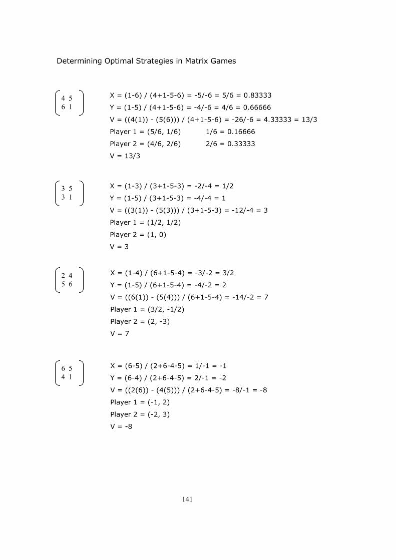
Determining Optimal Strategies in Matrix Games
141
X = (1-4) / (6+1-5-4) = -3/-2 = 3/2
Y = (1-5) / (6+1-5-4) = -4/-2 = 2
V = ((6(1)) - (5(4))) / (6+1-5-4) = -14/-2 = 7
Player 1 = (3/2, -1/2)
Player 2 = (2, -3)
V = 7
2 4
5 6
4 5
6 1
X = (1-6) / (4+1-5-6) = -5/-6 = 5/6 = 0.83333
Y = (1-5) / (4+1-5-6) = -4/-6 = 4/6 = 0.66666
V = ((4(1)) - (5(6))) / (4+1-5-6) = -26/-6 = 4.33333 = 13/3
Player 1 = (5/6, 1/6) 1/6 = 0.16666
Player 2 = (4/6, 2/6) 2/6 = 0.33333
V = 13/3
6 5
4 1
X = (6-5) / (2+6-4-5) = 1/-1 = -1
Y = (6-4) / (2+6-4-5) = 2/-1 = -2
V = ((2(6)) - (4(5))) / (2+6-4-5) = -8/-1 = -8
Player 1 = (-1, 2)
Player 2 = (-2, 3)
V = -8
3 5
3 1
X = (1-3) / (3+1-5-3) = -2/-4 = 1/2
Y = (1-5) / (3+1-5-3) = -4/-4 = 1
V = ((3(1)) - (5(3))) / (3+1-5-3) = -12/-4 = 3
Player 1 = (1/2, 1/2)
Player 2 = (1, 0)
V = 3

Determining Optimal Strategies in Matrix Games
142
Two intersecting points generate the same payoffs.
Optimal strategies and payoffs between;
Player 1 = (2/3, 1/3) and (1/2, 1/2)
Player 2 = (1, 0) and (1, 0)
V = 3
6 4
4 6
X = (6-4) / (6+6-4-4) = 2/4 = 1/2
Y = (6-4) / (6+6-4-4) = 2/4 = 1/2
V = ((6(6)) - (4(4))) / (6+6-4-4) = 20/4 = 5
Player 1 = (1/2, 1/2)
Player 2 = (1/2, 1/2)
V = 5
2 5
5 1
X = (1-5) / (3+2-5-3) = -4/-3 = 4/3
Y = (1-5) / (3+2-5-3) = -4/-3 = 4/3
V = ((2(1)) - (5(5))) / (3+1-5-3) = -23/-3 = 7.66666 = 23/3
Player 1 = (4/3, -1/3)
Player 2 = (4/3, -1/3)
V = 23/7
Determining Optimal Strategies in Matrix Games
143
Appendix F
Raw Results Output
This appendix contains all of the screen shots from the testing of the application.

Determining Optimal Strategies in Matrix Games
144
F.1. 2*2 Matrix Game Testing
Unit Test 1

Determining Optimal Strategies in Matrix Games
145

Determining Optimal Strategies in Matrix Games
146
Unit Test 2

Determining Optimal Strategies in Matrix Games
147

Determining Optimal Strategies in Matrix Games
148
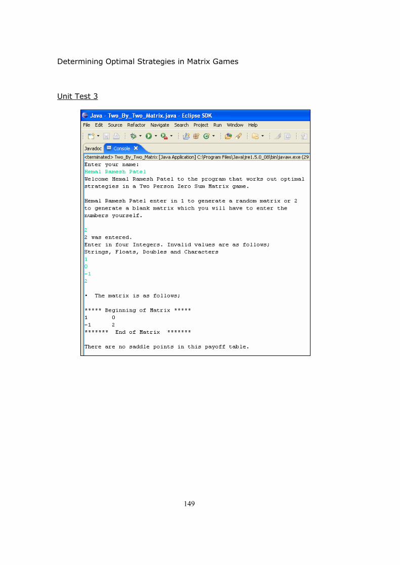
Determining Optimal Strategies in Matrix Games
149
Unit Test 3

Determining Optimal Strategies in Matrix Games
150

Determining Optimal Strategies in Matrix Games
151
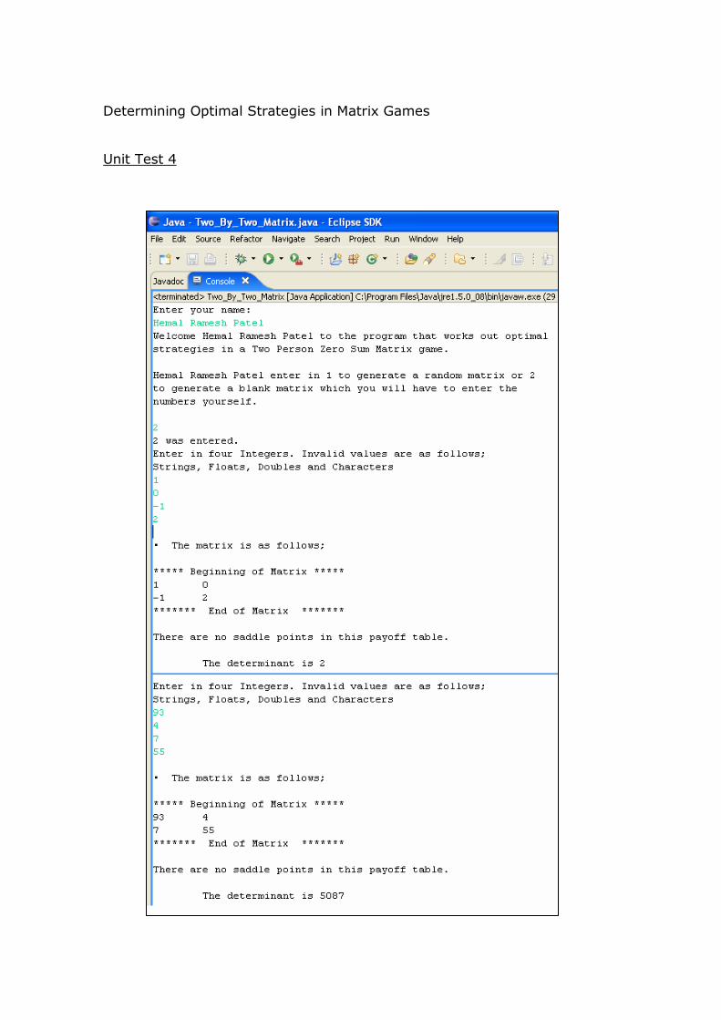
Determining Optimal Strategies in Matrix Games
152
Unit Test 4

Determining Optimal Strategies in Matrix Games
153
Unit Test 5
Unit Test 6
Unit Test 7
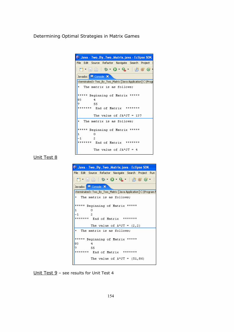
Determining Optimal Strategies in Matrix Games
154
Unit Test 8
Unit Test 9 – see results for Unit Test 4

Determining Optimal Strategies in Matrix Games
155
Unit Test 10

Determining Optimal Strategies in Matrix Games
156
Unit Test 11
Unit Test 12

Determining Optimal Strategies in Matrix Games
157
System Test

Determining Optimal Strategies in Matrix Games
158

Determining Optimal Strategies in Matrix Games
159

Determining Optimal Strategies in Matrix Games
160
F.2. 2*N Matrix Game Testing
Unit Test 1

Determining Optimal Strategies in Matrix Games
161
Unit Test 2

Determining Optimal Strategies in Matrix Games
162
Unit Test 3

Determining Optimal Strategies in Matrix Games
163
Unit Test 4

Determining Optimal Strategies in Matrix Games
164

Determining Optimal Strategies in Matrix Games
165
Unit Test 5

Determining Optimal Strategies in Matrix Games
166

Determining Optimal Strategies in Matrix Games
167
Unit Test 6
Unit Test 7

Determining Optimal Strategies in Matrix Games
168
Additional Testing
This appendix contains the extra 2*5 matrices that were used for additional testing.

Determining Optimal Strategies in Matrix Games
169
G.1 Additional 2*5 Matrices