ORIGINAL PAPER

Determining optimum number of geotechnical testing samplesusing Monte Carlo simulations

Kerry Magner1 & Norbert Maerz2 & Ivan Guardiola3 & Adnan Aqeel4

Received: 23 May 2016 /Accepted: 30 August 2017 /Published online: 16 September 2017# Saudi Society for Geosciences 2017

Abstract Knowing how many samples to test to adequatelycharacterize soil and rock units is always challenging. A largenumber of tests decrease the uncertainty and increase the con-fidence in the resulting values of design parameters.Unfortunately, this large value also adds to project costs.This paper presents a method to determine the number ofsamples as a function of the coefficient of variation. If, as inthe case of a reliability-based design, the resistance factors area function of the coefficient of variation of the measurements,then lowering the coefficient of variation (COV) can result inlowering of the resistance factor resulting in a less conserva-tive design. In this study, laboratory samples were isolated byspecific unified soil classification system soil type and generalsite location. A distribution was fitted for each of the geotech-nical parameters measured. For each scenario, groups of 2, 3,4, 5, 10, 15, 20, 30, 50, and 100 random samples were gener-ated by using Monte Carlo simulations from the fitted distri-butions. For each group, the variability was calculated interms of the COV. In all cases, the COV decreased as thesample size increased. However, the rate of decrease for the

COV was the greatest at a low number of samples; it becomesincreasingly smaller at a higher number of samples.

Keywords Geotechnical tests . Reliability .

Variance analysis . Sampling .Monte Carlomethod

Introduction

During geotechnical site investigations, both in situ and labo-ratory testingmethods are used to determine the geomechanicalcharacteristics of a soil/rock-type/location for the purpose ofgeotechnical design. In general, more reliable, less variabletesting results should translate into reduced uncertainty and aless conservative design, thus allowing cost savings in not onlythe design but also the construction process.

A site investigation engineer must determine how manysamples need to be tested to adequately characterize a site with-in a desired level of accuracy of the results. In making thisdetermination, the engineer must consider the purpose of thestudy, the population size, the risk involved in selecting a Bbad^sample, and the allowable sampling error. Three primarycriteria must be specified to determine the appropriate samplesize: the level of precision, the level of confidence (or risk), andthe degree of variability (Miaoulis and Michener 1976). Thelevel of precision is often referred as the sampling error that isthe range in which the true value of the population is to beestimated. The level of confidence (or risk) is based on the ideaof the central limit theorem. This theorem states that as a pop-ulation is repeatedly sampled, the average value of the attributeobtained is equal to the true population value. Finally, the de-gree of variability in the attributes being measured refers to thedistribution of attributes within the population. Hence, themoreheterogeneous a population is, the larger the sample size re-quired to obtain a given level of precision (Kish 1965;

* Adnan Aqeelben_aqeel_2005@yahoo.com

1 NewFields Mining Design and Technical Services, 225 Silver Street,Elko, NV 89801, USA

2 Department of Geological Sciences and Engineering, MissouriUniversity of Science and Technology, 1006 Kingshighway,Rolla, MO 65409-0660, USA

3 Department of Engineering Management, Missouri University ofScience and Technology, 1006 Kingshighway,Rolla, MO 65409-0660, USA

4 Department of Geology, Taibah University, Madinah 30002, SaudiArabia

Arab J Geosci (2017) 10: 406DOI 10.1007/s12517-017-3174-y

Cochran 1963). Each of these three criteria plays an importantrole in determining sample size. Typically, the number of sam-ples and tests is determined by engineering judgment and/orbudgetary considerations.

Several studies have been conducted across academicfields and applications to better understand this issue. Thesefield areas include, but are not limited to, industrial metrology(Owen and George 1957), industrial quality control(Quesenberry 1993), both biology and educational psycholo-gy (Clarke and Green 1988), engineering, political polling,and still other areas in which determining significance froma small representative sample is necessary due to the cost of afull population sample (Dowdy et al. 2004; Kachingan 1991).Krejcie andMorgan (1970) developed a chart for easy use andreference that can assist researchers in determining samplesize for various research tasks and activities. The use of thesemethods is not universal; a thorough understanding of thegoals and analysis task is highly required to employ suchcharts.

This paper presents an analytically based method to deter-mine the number of samples/test required based on statisticalanalysis for specific parameters. The interest lies in determin-ing the effects the sampling frequency (sample size) has or,essentially, how the number of geomechanical laboratory/insitu tests performed impacts the mean, variance, and coeffi-cient of variation of the individual geomechanical parameterwithin a defined soil/rock unit.

Variability, uncertainty, and reliability

The geotechnical variability of individual homogeneous iso-tropic soil/rock units is of interest when determining adequategeotechnical design parameters for most construction projects.Highly variable soil/rock laboratory testing results increasethe degree of uncertainty for geoengineers. Natural variabilityin the geological units, sampling errors (non-representativesampling), and sample storage, preparation, and testing pro-cedures can influence the variability of the laboratory testingresults. Both sampling and testing procedures can be opti-mized to reduce variability. However, natural variation is stillpresent.

Models of the subsurface conditions are generated fromeither direct or indirect site investigation techniques and asso-ciated laboratory testing. The geomechanical properties ob-tained, however, are uncertain in many aspects due to siteheterogeneities, measurement inaccuracies, along with datainconsistencies (Baecher and Christian 1972, 2003). To obtaina reliable site characterizationmodel, the uncertainties must bereduced and taken into account by the engineer (Schlager andSchonhardt 2008).

In general, as the number of samples tested increases, var-iability decreases; and thus, the uncertainty decreases resultingin increasing reliability. The law of large number implies that

as a sample becomes larger, the statistical properties of thesample are more accurately to resemble the population fromwhich the sample was taken (Baecher and Christian 2003).

Schlager and Schonhardt (2008) used a similar approach toquantifying uncertainty by use of a model composed of analgorithm and data arrangements in a theoretical variogramfor use in risk assessment of a tailings dam facility. Resultsfrom Schlager and Schonhardt (2008) research showed thatfor the model generated, further sampling and testing provideda maximal reduction in uncertainties up to a scope-relatedlevel; the model is then revised and the uncertainties furtherreduced.

Goldsworthy et al. (2007) performed a foundation designmodel simulation incorporated into a Monte Carlo frameworkto look at the expected costs (investigation, laboratory testing,and construction) and measure the financial risks associatedwith soil property variability and uncertainties. This simula-tion was performed on a simulated soil, where all thegeomechanical properties of the soils are known, a luxury thatis not attainable when using real soil sites. From this research,it was reported that the risks associated with variability anduncertainties can be reduced as the scope of the subsurfaceinvestigation is increased. However, there is a point identifiedas the optimal site investigation expenditure (Goldsworthyet al. 2007) where additional sampling becomes redundantand does not reduce the financial risks.

Reliability-based design

Reliability-based designs have evolved in engineering to ac-count for variability. For example, traditional calculations forfactor of safety are based on terms that have associated uncer-tainty (Duncan 2000). Load and resistance factor design(LRFD), popular in structural engineering and, more recently,in geotechnical engineering, redistributes factor of safety into

Fig. 1 Resistance factors for bearing resistance of spread footingfoundation on rock (MODOT 2011)

406 Page 2 of 19 Arab J Geosci (2017) 10: 406

separate load and resistance factors (Kulhawy and Phoon2002). LRFD equations take the general form that the requiredstrength equals the ultimate strength multiplied by the resis-tance factor, where the resistance factor with values between 0and 1.0 reflects the uncertainty.

An example of LRFD design guidelines, including the se-lection of resistance factors, is that presented by the MissouriDepartment of Transportation (MODOT) (2011) for drilledshafts, spread footings, and earth slopes (MODOT 2011).Figure 1 is an example of a design chart that relates the resis-tance factor (φ) to the variability in the form of the coefficientof variation of uniaxial compressive strength.

Relationship between variability and number of samples

The standard deviation is a measurement of the Bvariability^in statistical analysis that is used to gain inference regardingthe Bdispersion^within a sample of data. One common mis-conception is that increasing the sample size reduces thestandard deviation. However, it is the standard error, whichis directly affected by the sample. Consider taking a randomsample of 1000 samples from the common normal distribu-tion, with μ = 10, σ2 = 5. A basic calculation of both thestandard deviation and the standard error is taken from asubset of samples. Beginning the sample size at two and

Fig. 2 Standard error andstandard deviation as sample sizeincreases. Samples were takenfrom a normal distribution withmean of 10 and standarddeviation of 5 (N (10, 5)). It canbe observed that as the samplesize increases, the value of thestandard deviation oscillatesabout the actual value of 5. Thestandard error decreasescontinuously

Fig. 3 Study area location (kcICON Project) in an aerial layout, Kansas City (Google Earth). The geotechnical design was broken into two separatesegments (Segment 1 and Segment 2) separated by the Missouri River

Arab J Geosci (2017) 10: 406 Page 3 of 19 406

increasing it by four samples. Hence, the standard deviationis calculated at a sample size of {2, 6, 10, 14, n−4, n}. Thissimple calculation illustrates that the standard deviation willnot decrease as the sample size increases because the samplestandard deviation is a measure of the variability of a singleitem. In contrast, the standard error is a measure of the vari-ability of the average of all the items in the sample.

It can be easily observed that as the sample size increases,the value of the standard deviation oscillates about the actualvalue of 5. The standard error decreases continuously.

Figure 2 depicts the behavior of the standard deviationand the sample standard error as the sample size is in-creased. It illustrates that the standard error decreases con-tinuously as well as the standard deviation with an excep-tion that the later only oscillates about the actual value of5. Hence, it is more important to focus on reduction of thestandard error. The standard error (Se) of a sample size (n)is the sample standard deviation (σ) divided by the valueof

ffiffiffi

np

, which can be denoted by the following:

se ¼ σffiffiffi

np ð1Þ

The standard error estimates the standard deviation ofthe sample mean based on the population mean which isbasically affected by sample size. Therefore, it is highlyimportant to note that an inflection point exists at whichincreasing the sample size results in marginal gains in theapproximation of both the standard deviation and the stan-dard error. For example, increasing the sample size from60 to 120 (Fig. 2) produces a marginal reduction return ata high cost. Hence, the utility of increasing the samplesize decreases rapidly. Each experiment will have itsown inflection point. It is highly relevant to exploremethods to determine this inflection point for geotechni-cal experiments.

Objectives of this research

The main objective of this research project is to quantify thevariability of a geotechnical design parameter as a function ofsampling and testing frequency for different types of geotech-nical tests, soil types, and material conditions.

Methodology

The following methodologies for data reduction and analysiswere established to achieve the project objectives:

– Acquire a large data set of geotechnical in situ and labo-ratory test data;

– Divide the database into homogeneous soil and geo-graphic classification units;

– Determine the statistical distributions of each test, in eachclassification unit (a-priori identification of soil units);

– Perform Monte Carlo simulation with incrementally in-creasing sampling frequency (sample size);

– Calculate and plot mean, variance, and coefficient of var-iation for each random sampling scenario;

– Establish a tentative relationship between sample size andresistance factors for selected applications.

Table 1 Geotechnical testing conducted by Terracon

Testing method Number of tests

Direct shear testing 10

Consolidation testing 13

CU triaxial compression testing 8

UU triaxial compression testing 6

Unconfined compressive strength testing 87

Standard penetration testing 2115

Pocket penetrometer testing 551

Table 2 Test methods and associated geotechnical properties (Bardet1997)

Testing Method Property

Direct shear testing Friction angle (φ)—estimateof shear strength

Consolidation testing Overconsolidation ratio—estimateof the state of stress of cohesivematerials

CU triaxialcompression testing

Friction angle (φ)—estimateof shear strength

UU triaxialcompression testing

Undrained shear strength(Su)—estimate of shearstrength

Unconfined compressivestrength testing

Unconfined compressivestrength (Qu)—estimateof the undrained shearstrength

Standard penetration testing Index tests. SPT value(N)—estimate of the relativedensity of granular materials.Correlations with strengthsof cohesive materials.

Pocket penetrometer testing Unconfined compressive strength(Qu)—estimate of the undrainedshear strength

406 Page 4 of 19 Arab J Geosci (2017) 10: 406

Study area

The study area can be known as the project of KansasCity Interstate Connection (KcICON) (Fig. 3). The dataset of this project was used for the purpose of this re-search. This project consisted of reconstructing and wid-ening of approximately 4 miles of Interstate 29/35 in theMetro North Kansas City, Missouri, area. It included im-provements to numerous outdated interchanges, the con-struction of new interchange alignments, widening ofexisting highway pavement systems, numerous mechani-cally stabilized earthen (MSE) wall systems, numerousnoise wall (sound and light pollution reduction) systems,

and replacement of the existing Paseo Bridge over theMissouri River. It began at the confluence of Interstate29/35 with Interstate 70 and continued north of approx-imately 4.5 miles to just past the intersection of Interstate29/35 and Armor Road, as illustrated in Fig. 3.

Terracon Consultants, Inc. (Terracon) of Lenexa,Kansas, performed subsurface exploration as part of thegeotechnical research and design portion. This work wasconducted between January and October 2008. The geo-technical design was broken into two separate segments:Segment 1 (North Segment) and Segment 2 (SouthSegment). These segments were separated by theMissouri River (Fig. 3).

Fig. 4 Sample mean values forunconfined compressive strength.Top: fill materials. Bottom:cohesive materials

Arab J Geosci (2017) 10: 406 Page 5 of 19 406

Subsurface exploration

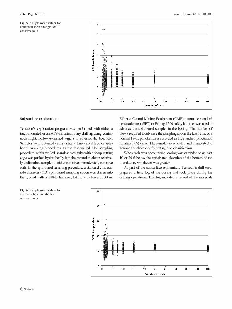
Terracon’s exploration program was performed with either atruck-mounted or an ATV-mounted rotary drill rig using contin-uous flight, hollow-stemmed augers to advance the borehole.Samples were obtained using either a thin-walled tube or split-barrel sampling procedures. In the thin-walled tube samplingprocedure, a thin-walled, seamless steel tube with a sharp cuttingedge was pushed hydraulically into the ground to obtain relative-ly undisturbed samples of either cohesive ormoderately cohesivesoils. In the split-barrel sampling procedure, a standard 2 in. out-side diameter (OD) split-barrel sampling spoon was driven intothe ground with a 140-lb hammer, falling a distance of 30 in.

Either a Central Mining Equipment (CME) automatic standardpenetration test (SPT) or Falling 1500 safety hammerwas used toadvance the split-barrel sampler in the boring. The number ofblows required to advance the sampling spoon the last 12 in. of anormal 18-in. penetration is recorded as the standard penetrationresistance (N) value. The samples were sealed and transported toTerracon’s laboratory for testing and classification.

When rock was encountered, coring was extended to at least10 or 20 ft below the anticipated elevation of the bottom of thefoundation, whichever was greater.

As part of the subsurface exploration, Terracon’s drill crewprepared a field log of the boring that took place during thedrilling operations. This log included a record of the materials

Fig. 6 Sample mean values foroverconsolidation ratio forcohesive soils

Fig. 5 Sample mean values forundrained shear strength forcohesive soils

406 Page 6 of 19 Arab J Geosci (2017) 10: 406

encountered during drilling as well as the driller’s interpretationof the subsurface conditions between the samples.

Geology

In general, Terracon characterized the subsurface using 120test borings from the Segment 1and 103 borings from theSegment 2 (Magner 2010). Four types of materials were iden-tified from the youngest (at the top) to the oldest (at the bot-tom) as the following: fill material, cohesivematerial, granularmaterial, and bedrock material. A brief description for eachmaterial type as follows:

i. The fill material consists of dark brown, brown, graybrown, yellowish brown, and greenish gray, lean to fatclay with varying amounts of silt, sand, gravel, and con-struction debris. This debris was comprised of concrete,brick, wood, charcoal, and glass.

ii. The cohesive material consists of brown and gray, lean tofat clay with varying amounts of silt, sand, and gravel.

iii. The granular material consists of light brown and brown,fine to medium sand with varying amounts of silt andclay.

iv. The bedrock, which lies underneath the other materials,consists of limestone overlying shale having different de-grees of weathering.

Fig. 7 Sample mean values forfriction angle (φ). Top: fillmaterials. Bottom: cohesivematerials

Arab J Geosci (2017) 10: 406 Page 7 of 19 406

Laboratory testing

Terracon conducted laboratory testing to investigate the engi-neering properties of the subsurface soils and rock. Accordingto Terracon’s Geotechnical Design Report (GDR) for Segment1 and Segment 2 of the kcICON project, the laboratory testingwas performed according to the ASTM standards. These testswere sieve analysis, moisture content, unit weight, pH,Atterberg limits, consolidation, standard proctor, unconfinedcompressive strength, direct shear, triaxial, and resistivity(Table 1). For the purpose of this study, only data from con-solidation, unconfined compressive strength, and direct sheartesting was used.

The bias error (i.e., sample disturbance) and random mea-surement error (i.e., instrument and operator error) are consid-ered to be insignificant compared to the inherent natural var-iability of the soils’ geomechanical properties. Therefore, thetotal measurement error in this laboratory data is considered tobe negligible and all variation is associated entirely with thesoils’ geomechanical properties.

Soil classification units

A visual analysis of the original geotechnical boring logs in-dicated that many different types of material are present within

Fig. 8 Sample mean values for STP blow-counts. Top: fill materials. Upper middle: cohesive materials. Lower middle: clayey sands.Bottom: clean sands

406 Page 8 of 19 Arab J Geosci (2017) 10: 406

the subsurface of the kcICON site. The geotechnical databasemust be separated into definable stratigraphic units to deter-mine the geotechnical variability of individual homogeneoussoil units. Within the Terracon boring logs, subsurface mate-rials with the exception of fill materials were classified accord-ing to the Unified Soil Classification System (USCS).Cohesive materials (fine soils) and cohesionless or granularmaterials (coarse soils) were identified.

The cohesive/fine grained soils included both of clay (C)and silt (M). This cohesive soil classified into the followingtypes of soils: fat clay (CH, clay with high plasticity), lean clay(CL, clay with low plasticity), a lean to fat clay (CL to CH),

silt with low plasticity (ML), and finally, a silty to clayey soilwith low plasticity (CL to ML).

Sandy soil was identified as the coarse soils in the studyarea. Both of poorly graded sand (SP) and well-gradedsand (SW) were identified in the area. Each of these twotypes of sands has a fine particle percentage (silt and/orclay) less than 5%, and thus, it is known as clean sand.Moreover, a silty to clayey sand (SM to SC), which is asand containing 5–12% of fine particles, was identified.Finally, both silty sand (SM) and clayey sand (CL), sandcontaining more than 12% of fine particles, were identifiedin the area.

Fig. 8 (continued)

Arab J Geosci (2017) 10: 406 Page 9 of 19 406

Geotechnical testing parameters and fittingdistributions

Geotechnical parameters

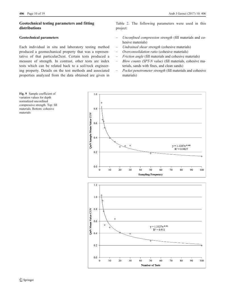
Each individual in situ and laboratory testing methodproduced a geomechanical property that was a represen-tative of that particular2test. Certain tests produced ameasure of strength. In contrast, other tests are indextests which can be related back to a soil/rock engineer-ing property. Details on the test methods and associatedproperties analyzed from the data obtained are given in

Table 2. The following parameters were used in thisproject:

– Unconfined compression strength (fill materials and co-hesive materials)

– Undrained shear strength (cohesive materials)– Overconsolidation ratio (cohesive materials)– Friction angle (fill materials and cohesive materials)– Blow counts (SPT-N value) (fill materials, cohesive ma-

terials, sands with fines, and clean sands)– Pocket penetrometer strength (fill materials and cohesive

materials)

Fig. 9 Sample coefficient ofvariation values for depthnormalized unconfinedcompressive strength. Top: fillmaterials. Bottom: cohesivematerials

406 Page 10 of 19 Arab J Geosci (2017) 10: 406

Fitting distributions to the geotechnical parameters

The original project methodology envisioned the randomsampling of a distinct geomechanical property value fromindividual strata within the created geotechnical database.For example, the unconfined compressive strength of thecohesive material for sample number X would be random-ly selected from the geotechnical database. It was deter-mined that this method of random sampling created a biasas each value had the same opportunity as any other to besampled, regardless of the frequency within the popula-tion. Thus, values with a very low sample frequency (i.e.,

outliers) had the equipotential to be sampled as did meanvalues.

All samples in this study were taken from a represen-tative distribution of the overall sampled population toremove bias. Either this population included the distinctgeomechanical property from the individual strata indicat-ed above or the laboratory testing data for a given lab teston a given soil type is used.

The determination of histograms and statistical distri-butions for each geomechanical property population wasperformed with Minitab-15® statistical analysis software.This allowed importing Excel data from the geotechnical

Fig. 10 Sample coefficient ofvariation values for depthnormalized undrained shearstrength for cohesive soils

Fig. 11 Sample coefficient ofvariation values foroverconsolidation ratio forcohesive soils

Arab J Geosci (2017) 10: 406 Page 11 of 19 406

database for computational analysis, histograms, and sta-tistical distribution determination.

Goodness-of-fit test

Minitab-15 software was utilized to analyze statistically theinput data. This analysis is to determine population size, mean,standard deviation, median value, minimum value, maximumvalue, skewness (a measure of asymmetry of the population),and kurtosis (a measure of Bpeakedness^ of the population).The Minitab-15 was then instructed to execute a goodness-of-fit test to identify how well a specific distribution fit the givenpopulation (Minitab Inc. 2010).

The measured goodness-of-fit (or p value) typicallysummarizes the difference between the population valuesand the values for the distribution in question. From this,it is determined that the greater the value from thegoodness-of-fit test, the greater the likelihood that the dis-tribution is a proper representation of the original popula-tion. In the Minitab-15 software, goodness-of-fit testingwas performed for many different types of distributionsincluding normal, lognormal, gamma, Weibull, logistic,log-logistic, and many variations/transformations of eachpopulation. In each case, the type of distribution that hadthe best goodness-of-fit was used. In most cases, this wasthe lognormal distribution.

Fig. 12 Sample coefficient ofvariation values for friction angle(φ). Top: fill materials. Bottom:cohesive materials

406 Page 12 of 19 Arab J Geosci (2017) 10: 406

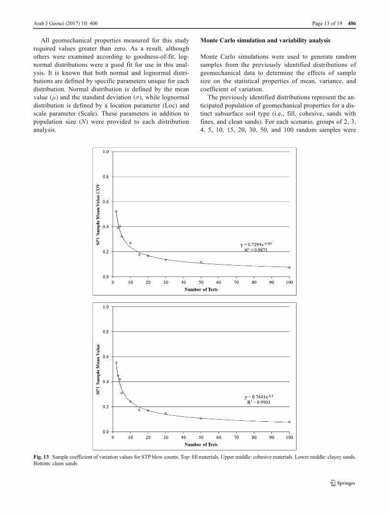
All geomechanical properties measured for this studyrequired values greater than zero. As a result, althoughothers were examined according to goodness-of-fit, log-normal distributions were a good fit for use in this anal-ysis. It is known that both normal and lognormal distri-butions are defined by specific parameters unique for eachdistribution. Normal distribution is defined by the meanvalue (μ) and the standard deviation (σ), while lognormaldistribution is defined by a location parameter (Loc) andscale parameter (Scale). These parameters in addition topopulation size (N) were provided to each distributionanalysis.

Monte Carlo simulation and variability analysis

Monte Carlo simulations were used to generate randomsamples from the previously identified distributions ofgeomechanical data to determine the effects of samplesize on the statistical properties of mean, variance, andcoefficient of variation.

The previously identified distributions represent the an-ticipated population of geomechanical properties for a dis-tinct subsurface soil type (i.e., fill, cohesive, sands withfines, and clean sands). For each scenario, groups of 2, 3,4, 5, 10, 15, 20, 30, 50, and 100 random samples were

Fig. 13 Sample coefficient of variation values for STP blow counts. Top: fill materials. Upper middle: cohesive materials. Lower middle: clayey sands.Bottom: clean sands

Arab J Geosci (2017) 10: 406 Page 13 of 19 406

generated from these distributions by Mathematica 7®.These groups of random samples were exported to Excelto generate graphs and variance analysis. Figures 4, 5, 6,7, 8 illustrate the results of the sampling in terms of themean values.

Variability was measured in terms of the coefficient ofvariation (COV), a normalized measure of variability(standard deviation/mean). This allowed for a comparisonbetween different data sets with varying means and evendifferent measurement units. Figures 9, 10, 11, 12, 13illustrate the results of the sampling in terms of the COV.

Results

Unconfined compression testing (QuN)—fill materialsand cohesive materials

Unconfined compression testing is a method used to estimate theunconfined compressive strength (Qu) of cohesive materials.Materials at shallow depths typically have a lower Qu whencompared to materials at greater depths. The samples used in thisstudy were normalized for depth to create unconfined compres-sive strength normalized for depth (QuN). In an effort to reduce

Fig. 13 (continued)

406 Page 14 of 19 Arab J Geosci (2017) 10: 406

the effect of depth on Qu, the Qu was divided by the effectiveoverburden stress (σ’) at the location depth of the sample.

A review of the goodness-of-fit test indicated that a lognor-mal distribution is a good representation of the QuN popula-tion. Figure 14 illustrates the histogram and the lognormaldistribution for QuN within fill materials and cohesive mate-rials, respectively.

Higher values of QuN (> 12) within the fill materials maypossibly be attributed to the controlled placement of fill

materials, possible cementation between fill material particles,or other foreign matter. No documentation was available re-garding how past fills were placed.

Undrained shear strength (SuN)—cohesive materials

Unconsolidated undrained (UU) triaxial test is a method usedto estimate the undrained shear strength (Su) of cohesive ma-terials. Similar to Qu, Su is also subject to the effects of depth.

Fig. 14 Lognormal fitted distribution of depth normalized unconfinedcompressive strength. Top: fill materials. Bottom: cohesive materials

Fig. 16 Lognormal fitted distribution of overconsolidation ratio forcohesive soils

Fig. 15 Lognormal fitted distribution of depth normalized undrainedshear strength for cohesive soils

Fig. 17 Lognormal fitted distribution of friction angle (φ). Top: fillmaterials. Bottom: cohesive materials

Arab J Geosci (2017) 10: 406 Page 15 of 19 406

The samples used in this study were normalized for depth tocreate undrained shear strength normalized for depth (SuN). Inan effort to reduce the effects of depth on Su, the Su wasdivided by the effective overburden stress (σ’) at the locationdepth of the sample.

A review of the goodness-of-fit test indicated that a lognor-mal distribution is a good representation of the population ofSuN. Figure 15 presents both the histogram and lognormaldistribution for SuN within a cohesive material.

Overconsolidation ratio—cohesive materials

The ratio of maximum past stress to the present stress valueapplied in cohesive soil is known as the overconsolidationratio (OCR). This ratio can be determined performing consol-idation test. A normally consolidated soil has a ratio equal toone; an overconsolidated soil has a ratio greater than one.Overconsolidation is typically resulting from some geologicalfactors such as the removal of overburden, glaciation process,and/or groundwater level fluctuation (Craig 2008).

A review of the goodness-of-fit test indicated that a lognor-mal distribution is a good representation of the population of

OCR. Figure 16 depicts both the histogram and lognormaldistribution for OCR within a cohesive material.

Friction angle (φ)—fill materials and cohesive materials

Both consolidated undrained (CU) triaxial testing and directshear (DS) testing were used to determine the friction angle(φ) of fill materials and cohesive soils. The shear resistance(shear strength) is a function of friction (angle) andinterlocking of the soil particles (Bardet 1997).

Different laboratory testing methods can influence the fric-tion angle within cohesive materials. Kulhawy and Mayne(1990) provided evidence that the relationship between φDS/φCU is equal to 1.22.

A review of the goodness-of-fit test indicated that a normaldistribution is a good representation of the population of φ infill material. A lognormal distribution was also found to be agood representation of the population of φ in a cohesive ma-terial. The normal distribution of the φ in a fill material maybe attributed to either the uniform placement of fill materialsduring construction or the small sample size (seven samples).Figure 17 illustrates the histogram and distribution forφwith-in fill materials and cohesive materials, respectively.

Fig. 18 Lognormal fitted distribution of STP blow-counts. Top: fill materials. Upper middle: cohesive materials. Lower middle: clayey sands.Bottom: clean sands

406 Page 16 of 19 Arab J Geosci (2017) 10: 406

Standard penetration testing—fill materials, cohesivematerials, sands with fines, and clean sands

Standard penetration testing (SPT) is a method used to esti-mate the relative density of granular materials. The number ofblows required to advance the sampling spoon the last 12 in.of a normal 18 in. penetration is recorded as the standardpenetration resistance (SPT-N) value. This value can also becorrelated with the relative density of cohesive materials aswell as with their strengths.

It has been noticed that the SPT-N values have not beencorrected for hammer energy, drill rod length, and/or overbur-den stress. It is found that during performing this test, the SPT-N value exceeded the acceptable limits (greater than 50) whenencountering obstruction such as rock fragments as in fill ma-terials or bedrocks as in cohesive and granular (sand) mate-rials. As a result, only those values were not used and deletedfrom the analysis.

A review of the goodness-of-fit test indicated that a lognor-mal distribution is a good representation of the populations ofthe SPT-N values. Figure 18 presents both the histograms andthe lognormal distributions for the SPT-N values within eachtype material.

Pocket penetrometer testing—fill materials

Pocket penetrometer testing is a method used to estimate theundrained shear strength of cohesive materials. This testingmethod is not only fast but also inexpensive. It is widely usedin the geotechnical industry.

A review of the goodness-of-fit test as well as the analysisof the population distribution indicated that there is no suffi-cient fit of a distribution to the population data. Figure 19depicts the histograms for PP values within the fill-type andcohesive-type materials.

Summary and conclusion

Summary

In this study, a soil database was created that containedsoil sampling and geotechnical laboratory testing datafrom the kcICON project has been created. Statistical dis-tributions of distinct individual geomechanical propertiesfor select soil and material types were established fromthis database. Next, a Brandom sample^ sampling scenariowith an incrementally increasing sampling frequency(sample size) was performed on the identified statisticaldistributions. Finally, statistical correlations of the mean,variance, and coefficient of variation were determined foreach Brandom sample^ sampling scenario.

In situ geotechnical soil sampling data and laboratory test-ing data were provided by Terracon Consultants, Inc. Thisprovided data was compiled into a database for use in furtheranalysis.

The original project methodology entailed the random sam-pling of a distinct geomechanical property value from individ-ual strata of the created geotechnical database. This method ofrandom sampling created a bias as each value had the potentialto be sampled regardless of the frequency within the popula-tion. Thus, values with a very low sample frequency (i.e.,outliers) had the equipotential to be sampled as did meanvalues.

All samples in this study were taken from a representativedistribution of the overall sampled population to remove bias.Either this population included the distinct geomechanicalproperty from the individual strata indicated above or the lab-oratory testing data for a given lab test on a given soil type isused. The computer Minitab-14 software was utilized to de-termine the distinct distributions for the individualgeomechanical properties of either the specific soil or materialtype.

The determined distributions represent the anticipated pop-ulation of geomechanical property for a distinct subsurfacesoil type (i.e., fill, cohesive, sands with fines, clean sands).

Fig. 19 Histogram of pocket penetrometer testing with no good fitteddistribution. Top: fill materials. Bottom: cohesive materials

Arab J Geosci (2017) 10: 406 Page 17 of 19 406

A Brandom sample^ sampling program was implemented todetermine the statistical variance of that population.Mathematica 7 computational software was employed to per-form a Brandom sample^ sampling scenario from the previ-ously established distributions.

Data from this Brandom sample^ sampling scenario wasthen analyzed to determine not only the mean values but alsothe variance and coefficient of variation of the mean values.

Conclusions

The following is a summary of the major conclusions present-ed in this paper:

– Depth, geological history, and soil type each influence thegeomechanical properties of a particular soil or material.The subsurface soils and materials must be separated intodistinct identifiable sub-strata before accurate compari-sons can be made between the geomechanical properties.

– Monte Carlo sampling from the list of distinct values oftest results was abandoned as it was found to be biased byoutliers. Instead, distinct distributions were generatedfrom the values of test results, and Monte Carlo samplingwas conducted on the measured distributions.

– In most of the test result values, the best fitting distribu-tion was the lognormal distribution, a distribution that isboth intuitive (no possible negative values) and easy towork with. Exceptions included both of the friction angleof fill materials (normal distribution) and the pocket pen-etrometer results for both fill and cohesive materials sincethere was no good fit found. The pocket penetrometerresults are not unexpected, as the distributions are skewedby the high number of measurements at the maximummeasureable level.

– Both variance calculations and COV calculations are re-spectable methods in determining the variability of aBrandom sample^ sampling program. COV determina-tion is useful in comparing the degree of variation be-tween different data sets, even if the mean values of eachindividual data set vary considerably.

– During the Monte Carlo simulations, it was observed thatthe variability decreased as the sampling frequencyincreased.

– It was also observed that there is a diminishing rate ofreturn on the decreased variability as a function of greatersampling frequency.

Application

The results of this research can be used to generalize the num-ber of samples based on one of two factors. The number ofsamples/tests can be determined by selecting a specific COV.

Not only that, but also the number of tests can be determinedby picking either a point of inflection on the curve or someother point at which additional samples/tests result in onlysmall decreases in variability.

For example, if a COVof 20% is selected (Figs. 9, 10, 11,12, 13), the resulting number of samples required is between12 and 19 for the different soil types. For cohesive soils, therequired number of tests of samples for undrained shearstrength testing and overconsolidation testing is 18 and 10,respectively. Moreover, 50 up to 100 samples would be re-quired for undrained compressive strength testing, while forfiction testing is not more than two samples.

In contrast, subjectively choosing a point of inflection thatis similar on all of the curves in Figs. 9, 10, 11, 12, 13 willresult in a requirement of 10 and 13 samples in all cases.

However, these results are generalization and should not beused to extrapolate from one site to another. Additionally, theycannot be generated in Breal time^ as the better fit to thepopulation distribution requires more test results rather thanfewer. A Breal time^ approach must also consider how fast thefitted distribution converges to the population distribution as afunction of the number of samples.

Acknowledgements The authors would like to deeply thank TerraconConsultants, Inc. for providing both of in situ and laboratory data samplesto be used in this research. The authors would also like to sincerely thankall of the Missouri Department of Transportation, Brian Kidwell (thekcICON project director), the Center for Transportation Infrastructureand Safety—a National University Transportation Center at MissouriUniversity of Science and Technology, and the Missouri University ofScience and Technology for funding this project and their valuablesupport.

References

Baecher GB, Christian T (1972) Site exploration: a probabilistic ap-proach. Dissertation, Massachusetts Institute of Technology

Baecher GB, Christian JT (2003) Reliability and statistics in geotechnicalengineering. John Wiley & Sons Ltd, England, 605 pp

Bardet JP (1997) Experimental soil mechanics. Prentice Hall, UpperSaddle

Clarke KR, Green RH (1988) Statistical design and analysis for aBbiological effects^ study. Mar Ecol Prog Ser 46(1–3):213–226

Cochran WG (1963) Sampling techniques, 2nd edn. John Wiley & SonsInc., New York

Craig RF (2008) Craig’s soil mechanics. Spon Press, London/New YorkDowdy S,Wearden S, ChilkoD (2004) Statistics for research. JohnWiley

& Sons Inc., Hoboken, New YorkDuncan M (2000) Factors of safety and reliability in geotechnical engi-

neering. J Geotech Geoenviron:307–316Goldsworthy JS, Jaska MB, Fenton GA, Griffiths DV, Kaggwa WS,

Poulos HG (2007) Measuring the risk of geotechnical site investi-gations. GeoDenver 2007: New Peaks in Geotechnics. AmericanSociety of Civil Engineers, GSP 170 Probabilistic Applications inGeotechincal Engineering 1–12

Kachingan SK (1991) Multivariate statistical analysis: a conceptual in-troduction, 2nd edn. Radius Press, New York

Kish L (1965) Survey sampling. John Wiley & Sons Inc., New York

406 Page 18 of 19 Arab J Geosci (2017) 10: 406

Krejcie RV,Morgan DW (1970) Determining the sample size for researchactivities. J Educ Psychol Meas 30(3):607–610

Kulhawy FH, Mayne PW (1990)Manual on estimating soil properties forfoundation design. Electric Power Research Institute, Palo Alto,Calif., Report EL-6800: Research Project 1493–6

Kulhawy FH, Phoon KK (2002) Observations on reliability-based designdevelopment in North America. Foundation design codes and soilinvestigation in view of international harmonization and perfor-mance. Balkema, Lisse, pp 31–48

Magner KA (2010) Characterization of geotechnical variability basedupon sampling frequency using a Monte Carlo simulation: a studyof the KciCON project. M.Sc. Thesis, Missouri University ofScience and Technology

Miaoulis G, Michener RD (1976) An introduction to sampling. Kendall/Hunt Publishing Company, Dubuque

Minitab Inc. (2010)Minitab statistical software (version 15). Minitab Inc.web. http://www.Minitab.Com. Accessed 1st June 2010

MODOT: TheMissouri Department of Transportation (2011) Proceduresfor estimation of geotechnical parameter values and coefficients ofvariation. IOP Publishing Engineering Policy Guide Web. http://epg.modot.org/index.php?title=321.3_Procedures_for_Estimation_of_Geotechnical_Parameter_Values_and_Coefficients_of_Variation#321.3.6.1_General. Accessed 10th June 2010

Owen LD, George EP (1957) Statistical methods in research production,with special reference to chemical industry, 3rd edn. Published forImperial Chemical Industries by Oliver and Boyd, London

Quesenberry CP (1993) The effect of sample size on estimated limits forsample mean and X control charts. J Qual Technol 25(4):237–237

Schlager P, Schonhardt M (2008) Optimized site investigation andrisk assessment strategies considering uncertain geotechnicalparameters using Geo-AllStaR. GeoCongress 2008. Am SocCivil Eng 573–580

Arab J Geosci (2017) 10: 406 Page 19 of 19 406