determining the epipolar geometry and its uncertainty: a...

P1: NTA

International Journal of Computer Vision KL553-03-ZHANG March 2, 1998 15:16

International Journal of Computer Vision 27(2), 161–195 (1998)c© 1998 Kluwer Academic Publishers. Manufactured in The Netherlands.

Determining the Epipolar Geometry and its Uncertainty: A Review

ZHENGYOU ZHANGINRIA, 2004 route des Lucioles, BP 93, F-06902 Sophia-Antipolis Cedex, France

[email protected]

Received July 16, 1996; Accepted February 13, 1997

Abstract. Two images of a single scene/object are related by the epipolar geometry, which can be described by a3×3 singular matrix called the essential matrix if images’ internal parameters are known, or the fundamental matrixotherwise. It captures all geometric information contained in two images, and its determination is very important inmany applications such as scene modeling and vehicle navigation. This paper gives an introduction to the epipolargeometry, and provides a complete review of the current techniques for estimating the fundamental matrix and itsuncertainty. A well-founded measure is proposed to compare these techniques. Projective reconstruction is alsoreviewed. The software which we have developed for this review is available on the Internet.

Keywords: epipolar geometry, fundamental matrix, calibration, reconstruction, parameter estimation, robusttechniques, uncertainty characterization, performance evaluation, software

1. Introduction

Two perspective images of a single rigid object/sceneare related by the so-calledepipolar geometry, whichcan be described by a 3×3 singular matrix. If the inter-nal (intrinsic) parameters of the images (e.g., the focallength, the coordinates of the principal point, etc.) areknown, we can work with thenormalized image coordi-nates(Faugeras, 1993), and the matrix is known as theessential matrix(Longuet-Higgins, 1981); otherwise,we have to work with thepixel image coordinates,and the matrix is known as thefundamental matrix(Luong, 1992; Faugeras, 1995; Luong and Faugeras,1996). It contains all geometric information that isnecessary for establishing correspondences betweentwo images, from which three-dimensional structureof the perceived scene can be inferred. In a stereovi-sion system where the camera geometry is calibrated,it is possible to calculate such a matrix from the cam-era perspective projection matrices through calibration(Ayache, 1991; Faugeras, 1993). When the intrinsicparameters are known but the extrinsic ones (the rota-tion and translation between the two images) are not,

the problem is known as motion and structure from mo-tion, and has been extensively studied in Computer Vi-sion; two excellent reviews are already available in thisdomain (Aggarwal and Nandhakumar, 1988; Huangand Netravali, 1994). We are interested here in differ-ent techniques for estimating the fundamental matrixfrom two uncalibrated images, i.e., the case where boththe intrinsic and extrinsic parameters of the images areunknown. From this matrix, we can reconstruct a pro-jective structure of the scene, defined up to a 4× 4matrix transformation.

The study of uncalibrated images has many impor-tant applications. The reader may wonder the useful-ness of such a projective structure. We cannot obtainany metric information from a projective structure:measurements of lengths and angles do not make sense.However, a projective structure still contains rich in-formation, such as coplanarity, collinearity, and crossratios (ratio of ratios of distances), which is sometimessufficient for artificial systems, such as robots, to per-form tasks such as navigation and object recognition(Shashua, 1994a; Zeller and Faugeras, 1994; Beardsleyet al., 1994).

P1: NTA


162 Zhang

In many applications such as the reconstruction ofthe environment from a sequence of video imageswhere the parameters of the video lens is submittedto continuous modification, camera calibration in theclassical sense is not possible. We cannot extract anymetric information, but a projective structure is stillpossible if the camera can be considered as a pin-hole. Furthermore, if we can introduce some knowl-edge of the scene into the projective structure, we canobtain more specific structure of the scene. For exam-ple, by specifying a plane at infinity (in practice, weneed only to specify a plane sufficiently far away), anaffine structure can be computed, which preserves par-allelism and ratios of distances (Quan, 1993; Faugeras,1995). Hartley et al. (1992) first reconstruct a pro-jective structure, and then use eight ground referencepoints to obtain the Euclidean structure and the cameraparameters. Mohr et al. (1993) embed constraints suchas location of points, parallelism and vertical planes(e.g., walls) directly into a minimization procedure todetermine a Euclidean structure. Robert and Faugeras(1993) show that the 3D convex hull of an object canbe computed from a pair of images whose epipolar ge-ometry is known.

If we assume that the camera parameters do notchange between successive views, the projective invari-ants can even be used to calibrate the cameras in theclassical sense without using any calibration apparatus(known asself-calibration) (Maybank and Faugeras,1992; Faugeras et al., 1992; Luong, 1992; Zhang et al.,1996; Enciso, 1995):

Recently, we have shown (Zhang, 1996a) that evenin the case where images are calibrated, more reliableresults can be obtained if we use the constraints arisingfrom uncalibrated images as an intermediate step.

This paper gives an introduction to the epipolar ge-ometry, provides a new formula of the fundamentalmatrix which is valid for both perspective and affinecameras, and reviews different methods reported in theliterature for estimating the fundamental matrix. Fur-thermore, a new method is described to compare twoestimations of the fundamental matrix. It is based on ameasure obtained through sampling the whole visible3D space. Projective reconstruction is also reviewed.The software calledFMatrix which implements thereviewed methods and the software calledFdiffwhich computes the difference between two fundamen-tal matrices are both available from my home page:

http://www.inria.fr/robotvis/personnel/

zzhang/zzhang-eng.html

FMatrix detects false matches, computes the funda-mental matrix and its uncertainty, and performs theprojective reconstruction of the points as well. Al-though not reviewed, a softwareAffineF which com-putes the affine fundamental matrix (see Section 5.3)is also made available.

2. Epipolar Geometry and Problem Statement

2.1. Notation

A camera is described by the widely used pinholemodel. The coordinates of a 3D pointM = [x, y, z]T

in a world coordinate system and its retinal image co-ordinatesm = [u, v]T are related by

s

uv

1

= P

xyz1

,wheres is an arbitrary scale, andP is a 3× 4 matrix,called the perspective projection matrix. Denoting thehomogeneous coordinates of a vectorx = [x, y, . . .]T

by x, i.e., x = [x, y, . . . ,1]T , we havesm = PM.The matrixP can be decomposed as

P= A[R t],

whereA is a 3×3 matrix, mapping the normalized im-age coordinates to the retinal image coordinates, and(R, t) is the 3D displacement (rotation and translation)from the world coordinate system to the camera coor-dinate system.

The quantities related to the second camera is indi-cated by′. For example, ifmi is a point in the firstimage,m′i denotes its corresponding point in the sec-ond image.

A line l in the image passing through pointm =[u, v]T is described by equationau+ bv+ c = 0. Letl = [a, b, c]T , then the equation can be rewritten aslTm = 0 or mT l = 0. Multiplying l by any non-zeroscalar will define the same 2D line. Thus, a 2D lineis represented by a homogeneous 3D vector. The dis-tance from pointm0 = [u0, v0]T to line l = [a, b, c]T

is given by

d(m0, l) = au0+ bv0+ c√a2+ b2

.

Note that we here use thesigneddistance.

P1: NTA


Epipolar Geometry 163

Finally, we use a concise notationA−T = (A−1)T =(AT )−1 for any invertible square matrixA.

2.2. Epipolar Geometry and Fundamental Matrix

The epipolar geometry exists between any two camerasystems. Consider the case of two cameras as shownin Fig. 1. LetC andC′ be the optical centers of the firstand second cameras, respectively. Given a pointm inthe first image, its corresponding point in the secondimage is constrained to lie on a line called theepipolarline of m, denoted byl′m. The linel′m is the intersec-tion of the plane5, defined bym, C andC′ (knownas theepipolar plane), with the second image planeI ′. This is because image pointm may correspond toan arbitrary point on the semi-lineCM (M may be atinfinity) and that the projection ofCM onI ′ is the linel ′m. Furthermore, one observes that all epipolar linesof the points in the first image pass through a commonpoint e′, which is called theepipole. Epipolee′ is theintersection of the lineCC′ with the image planeI ′.This can be easily understood as follows. For eachpointmk in the first imageI, its epipolar linel′mk

in I ′is the intersection of the plane5k, defined bymk, CandC′, with image planeI ′. All epipolar planes5k

thus form a pencil of planes containing the lineCC′.They must intersectI ′ at a common point, which ise′.Finally, one can easily see the symmetry of the epipolargeometry. The corresponding point in the first imageof each pointm′k lying on l′mk

must lie on the epipolarline lm′k , which is the intersection of the same plane5k

with the first image planeI. All epipolar lines forma pencil containing the epipolee, which is the inter-

Figure 1. The epipolar geometry.

section of the lineCC′ with the image planeI. Thesymmetry leads to the following observation. Ifm (apoint inI) andm′ (a point inI ′) correspond to a singlephysical pointM in space, thenm, m′, C andC′must liein a single plane. This is the well-knownco-planarityconstraintin solving motion and structure from motionproblems when the intrinsic parameters of the camerasare known (Longuet-Higgins, 1981).

The computational significance in matching differ-ent views is that for a point in the first image, its corres-pondence in the second image must lie on the epipolarline in the second image, and then the search space fora correspondence is reduced from two dimensions toone dimension. This is called theepipolar constraint.Algebraically, in order form in the first image andm′ in the second image to be matched, the followingequation must be satisfied:

m′TFm = 0 with F = A′−T [t]×RA−1, (1)

where(R, t) is the rigid transformation (rotation andtranslation) which brings points expressed in the firstcamera coordinate system to the second one, and [t]× isthe antisymmetric matrix defined byt such that [t]×x =t × x for all 3D vectorx. This equation can be derivedas follows. Without loss of generality, we assume thatthe world coordinate system coincides with the firstcamera coordinate system. From the pinhole model,we have

sm = A[I 0] M and s′m′ = A′[R t] M.

EliminatingM, s ands′ in the above two equations, weobtain Eq. (1). Geometrically,Fm defines the epipolarline l′m of point m in the second image. Equation (1)says no more than that the correspondence in the secondimage of pointm lies on the corresponding epipolar linel′m. Transposing (1) yields the symmetric relation fromthe second image to the first image:mTFTm′ = 0.

The 3×3 matrixF is called thefundamental matrix.Since det([t]×) = 0,

det(F) = 0. (2)

F is of rank 2. Besides, it is only defined up to a scalarfactor, because ifF is multiplied by an arbitrary scalar,Eq. (1) still holds. Therefore, a fundamental matrix hasonly seven degrees of freedom. There are only sevenindependent parameters among the nine elements ofthe fundamental matrix.

P1: NTA


164 Zhang

Convention Note. We use the first camera coordinatesystem as the world coordinate system. In (Faugeras,1993; Xu and Zhang, 1996), the second camera coor-dinate system is chosen as the world one. In this case,(1) becomesmTF′m′ = 0 with F′ = A−T [t′]×R′A′−1,where(R′, t′) transforms points from the second cam-era coordinate system to the first. The relation between(R, t) and(R′, t′) is given byR′ = RT , andt′ = −RTEt.The reader can easily verify thatF = F′T .

2.3. A General Form of Epipolar Equation for AnyProjection Model

In this section we will derive a general form of epipolarequation which does not assume whether the camerasfollow the perspective or affine projection model (Xuand Zhang, 1996).

A point m in the first image is matched to a pointm′ in the second image. From the camera projectionmodel (orthographic, weak perspective, affine, or fullperspective), we havesm = PM ands′m′ = P′M, whereP andP′ are 3×4 matrices. An image pointm definesactually an optical ray, on which every space pointMprojects on the first image atm. This optical ray canbe written in parametric form as

M = sP+m+ p⊥, (3)

whereP+ is the pseudo-inverse of matrixP:

P+ = PT (PPT )−1, (4)

andp⊥ is any 4-vector that is perpendicular to all therow vectors ofP, i.e.,

Pp⊥ = 0.

Thus,p⊥ is a null vector ofP. As a matter of fact,p⊥

indicates the position of the optical center (to which alloptical rays converge). We show later how to determinep⊥. For a particular values, Eq. (3) corresponds to apoint on the optical ray defined bym. Equation (3)is easily justified by projectingM onto the first image,which indeed givesm.

Similarly, an image pointm′ in the second imagedefines also an optical ray. Requiring that the two raysto intersect in space implies that a pointM correspond-ing to a particulars in (3) must project onto the second

image atm′, that is

s′m′ = sP′P+m+ P′p⊥.

Performing a cross product withP′p⊥ yields

s′(P′p⊥)× m′ = s(P′p⊥)× (P′P+m).

Eliminatings ands′ by multiplying m′T from the left(equivalent to a dot product), we have

m′TFm = 0, (5)

whereF is a 3× 3 matrix, calledfundamental matrix:

F = [P′p⊥]×P′P+. (6)

Sincep⊥ is the optical center of the first camera,P′p⊥

is actually the epipole in the second image. It can alsobe shown that this expression is equivalent to (1) for thefull perspective projection (see Xu and Zhang, 1996),but it is more general. Indeed, (1) assumes that the first3× 3 sub-matrix ofP is invertible, and thus is onlyvalid for full perspective projection but not for affinecameras (see Section 5.3), while (6) makes use of thepseudoinverse of the projection matrix, which is validfor both full perspective projection as well as affinecameras. Therefore, the equation does not depend onany specific knowledge of projection model. Replacingthe projection matrix in the equation by specific pro-jection matrix for each specific projection model (e.g.,orthographic, weak perspective, affine or full perspec-tive) produces the epipolar equation for that specificprojection model. See (Xu and Zhang, 1996) for moredetails.

The vectorp⊥ still needs to be determined. We firstnote that such a vector must exist because the differencebetween the row dimension and the column dimensionis one, and that the row vectors are generally indepen-dent from each other. Indeed, one way to obtainp⊥

is

p⊥ = (I − P+P)ω, (7)

whereω is an arbitrary 4-vector. To show thatp⊥ is per-pendicular to each row ofP, we multiplyp⊥ by P fromthe left: Pp⊥ = (P− PPT (PPT )−1P)ω= 0, which isindeed a zero vector. The action ofI −P+P is to trans-form an arbitrary vector to a vector that is perpendicularto every row vector ofP. If P is of rank 3 (which is the

P1: NTA



case for both perspective and affine cameras), thenp⊥

is unique up to a scale factor.

2.4. Problem Statement

The problem considered in the sequel is the estimationof F from a sufficiently large set of point correspon-dences: {(mi ,m′i ) | i = 1, . . . ,n}, wheren ≥ 7.The point correspondences between two images canbe established by a technique such as that describedin (Zhang et al., 1995). We allow, however, that a frac-tion of the matches may be incorrectly paired, and thusthe estimation techniques should be robust.

3. Techniques for Estimatingthe Fundamental Matrix

Let a pointmi = [ui , vi ]T in the first image be matchedto a pointm′i = [u′i , v

′i ]

T in the second image. Theymust satisfy the epipolar Eq. (1), i.e.,m′Ti Fmi = 0.This equation can be written as a linear and homo-geneous equation in the 9 unknown coefficients ofmatrixF:

uTi f = 0, (8)

where

ui = [ui u′i , vi u

′i , u′i , ui v

′i , vi v

′i , v′i , ui , vi , 1]T

f = [F11, F12, F13, F21, F22, F23, F31, F32, F33]T .

Fi j is the element ofF at row i and columnj .If we are givenn point matches, by stacking (8), we

have the following linear system to solve:

Unf = 0,

where

Un = [u1, . . . ,un]T .

This set of linear homogeneous equations, togetherwith the rank constraint of the matrixF, allow us toestimate the epipolar geometry.

3.1. Exact Solution with Seven Point Matches

As described in Section 2.2, a fundamental matrixFhas only 7 degrees of freedom. Thus, 7 is the minimum

number of point matches required for having a solutionof the epipolar geometry.

In this case,n= 7 and rank(U7)= 7. Through sin-gular value decomposition, we obtain vectorsf1 andf2

which span the null space ofU7. The null space is alinear combination off1 and f2, which correspond tomatricesF1 andF2, respectively. Because of its ho-mogeneity, the fundamental matrix is a one-parameterfamily of matricesαF1 + (1− α)F2. Since the deter-minant ofF must be null, i.e.,

det[αF1+ (1− α)F2] = 0,

we obtain a cubic polynomial inα. The maximumnumber of real solutions is 3. For each solutionα, thefundamental matrix is then given by

F = αF1+ (1− α)F2.

Actually, this technique has already been used in esti-mating the essential matrix when seven point matchesin normalized coordinates are available (Huang andNetravali, 1994). It is also used in (Hartley, 1994; Torret al., 1994) for estimating the fundamental matrix.

As a matter of fact, the result that there may havethree solutions given seven matches has been knownsince 1800’s (Hesse, 1863; Sturm, 1869). Sturm’s al-gorithm (Sturm, 1869) computes the epipoles and theepipolar transformation (see Section 2.2) from sevenpoint matches. It is based on the observation that theepipolar lines in the two images are related by a ho-mography, and thus the cross-ratios of four epipolarlines is invariant. In each image, the seven points de-fine seven lines going through the unknown epipole,thus providing four independent cross-ratios. Sincethese cross-ratios should remain the same in the twoimages, one obtains four cubic polynomial equationsin the coordinates of the epipoles (four independent pa-rameters). It is shown that there may exist up to threesolutions for the epipoles.

3.2. Analytic Method with Eightor More Point Matches

In practice, we are given more than seven matches.If we ignore the rank-2 constraint, we can use aleast-squares method to solve

minF

∑i

(m′Ti Fmi

)2, (9)

P1: NTA


166 Zhang

which can be rewritten as:

minf‖Unf‖2. (10)

The vectorf is only defined up to an unknown scalefactor. The trivial solutionf to the above problem isf = 0, which is not what we want. To avoid it, we needto impose some constraint on the coefficients of thefundamental matrix. Several methods are possible andare presented below. We will call themthe eight-pointalgorithm, although more than eight point matches canbe used.

3.2.1. Linear Least-Squares Technique.The firstmethod sets one of the coefficients ofF to 1, and thensolves the above problem using linear least-squarestechniques. Without loss of generality, we assume thatthe last element of vectorf (i.e., f9 = F33) is not equalto zero, and thus we can setf9 = −1. This gives

‖UnEf‖2 = ‖U′nf ′ − c9‖2

= f ′TU′Tn U′nf ′ − 2cT9 U′nf ′ + cT

9 c9,

whereU′n is then×8 matrix composed of the first eightcolumns ofUn, andc9 is the ninth column ofUn. Thesolution is obtained by requiring the first derivative tobe zero, i.e.,

∂‖Unf‖2∂f ′

= 0.

By definition of vector derivatives,∂(aTx)/∂x = a, forall vectora. We thus have

2U′Tn U′nf ′ − 2U′Tn c9 = 0,

or

f ′ = (U′Tn U′n)−1

U′Tn c9.

The problem with this method is that we do not knowa priori which coefficient is not zero. If we set anelement to 1 which is actually zero or much smallerthan the other elements, the result will be catastrophic.A remedy is to try all nine possibilities by setting oneof the nine coefficients ofF to 1 and retain the bestestimation.

3.2.2. Eigen Analysis. The second method consists inimposing a constraint on the norm off, and in particularwe can set‖f‖ = 1.Compared to the previous method,

no coefficient ofF prevails over the others. In this case,the problem (10) becomes a classical one:

minf‖Unf‖2 subject to‖f‖ = 1. (11)

It can be transformed into an unconstrained minimiza-tion problem through Lagrange multipliers:

minfF(f, λ), (12)

where

F(f, λ) = ‖Unf‖2+ λ(1− ‖f‖2) (13)

andλ is the Lagrange multiplier. By requiring the firstderivative ofF(f, λ) with respect tof to be zero, wehave

UTn Unf = λf.

Thus, the solutionf must be a unit eigenvector of the9× 9 matrixUT

n Un andλ is the corresponding eigen-value. Since matrixUT

n Un is symmetric and positivesemi-definite, all its eigenvalues are real and positiveor zero. Without loss of generality, we assume the nineeigenvalues ofUT

n Un are in non-increasing order:

λ1 ≥ · · · ≥ λi ≥ · · · ≥ λ9 ≥ 0.

We therefore have nine potential solutions:λ = λi fori = 1, . . . ,9. Back substituting the solution to (13)gives

F(f, λi ) = λi .

Since we are seeking to minimizeF(f, λ), the solutionto (11) is evidently the unit eigenvector of matrixUT

n Un

associated to thesmallesteigenvalue, i.e.,λ9.

3.2.3. Imposing the Rank-2 Constraint.The advan-tage of the linear criterion is that it yields an analytic so-lution. However, we have found that it is quite sensitiveto noise, even with a large set of data points. One rea-son is that the rank-2 constraint (i.e., detF = 0) is notsatisfied. We can impose this constraint a posteriori.The most convenient way is to replace the matrixF estimated with any of the above methods by thematrix F which minimizes the Frobenius norm (see

P1: NTA



Appendix, Section A.3.3) ofF− F subject to the con-straint detF = 0. Let

F = USVT

be the singular value decomposition of matrixF, whereS = diag(σ1, σ2, σ3) is a diagonal matrix satisfyingσ1 ≥ σ2 ≥ σ3 (σi is thei th singular value), andU andV are orthogonal matrices. It can be shown that

F = USVT

with S = diag(σ1, σ2, 0) minimizes the Frobeniusnorm of F − F (see the Appendix B for the proof).This method was used by Tsai and Huang (1984) inestimating the essential matrix and by Hartley (1995)in estimating the fundamental matrix.

3.2.4. Geometric Interpretation of the Linear Crite-rion. Another problem with the linear criterion isthat the quantity we are minimizing is not physicallymeaningful. A physically meaningful quantity shouldbe something measured in the image plane, because theavailable information (2D points) are extracted fromimages. One such quantity is the distance from a pointm′i to its corresponding epipolar linel′i = Fmi ≡[l ′1, l

′2, l′3]T , which is given by (see Section 2.1)

d(m′i , l′i ) =

m′Ti l′i√l ′21 + l ′22

= 1

c′im′Ti Fmi , (14)

wherec′i =√

l ′21 + l ′22 . Thus, the criterion (9) can berewritten as

minF

n∑i=1

c′2i d2(m′i , l′i ).

This means that we are minimizing not only a physicalquantityd(m′i , l

′i ), but alsoc′i which is not physically

meaningful. Luong (1992) shows that the linear crite-rion introduces a bias and tends to bring the epipolestowards the image center.

3.2.5. Normalizing Input Data. Hartley (1995) hasanalyzed, from a numerical computation point of view,the high instability of this linear method if pixel co-ordinates are directly used, and proposed to perform asimple normalization of input data prior to running theeight-point algorithm. This technique indeed producesmuch better results, and is summarized below.

Suppose that coordinatesmi in one image are re-placed bymi =Tmi , and coordinatesm′i in the otherimage are replaced bym′i =T′m′i , where T andT ′ are any 3× 3 matrices. Substituting in theequation m′Ti Fmi = 0, we derive the equationm′Ti T′−TFT−1mi = 0. This relation implies thatT′−TFT−1 is the fundamental matrix corresponding tothe point correspondencesmi ↔ m′i . Thus, an alter-native method of finding the fundamental matrix is asfollows:

1. Transform the image coordinates according to trans-formationsmi = Tmi andm′i = T′m′i .

2. Find the fundamental matrixF corresponding to thematchesmi ↔ m′i .

3. Retrieve the original fundamental matrix asF =T ′T FT.

The question now is how to choose the transformationsT andT′.

Hartley (1995) has analyzed the problem with theeight-point algorithm, which shows that its poor per-formance is due mainly to the poor conditioning of theproblem when the pixel image coordinates are directlyused (see Appendix C). Based on this, he has proposedan isotropic scaling of the input data:

1. As a first step, the points are translated so that theircentroid is at the origin.

2. Then, the coordinates are scaled, so that on the aver-age a pointmi is of the formmi = [1, 1, 1]T . Sucha point will lie at a distance

√2 from the origin.

Rather than choosing different scale factors foruand v coordinates, we choose to scale the pointsisotropically so that the average distance from theorigin to these points is equal to

√2.

Such a transformation is applied to each of the twoimages independently.

An alternative to the isotropic scaling is an affinetransformation so that the two principal moments ofthe set of points are both equal to unity. However,Hartley (1995) found that the results obtained werelittle different from those obtained using the isotropicscaling method.

Beardsley et al. (1994) mention a normalizationscheme which assumes some knowledge of camera pa-rameters. Actually, if approximate intrinsic parameters(i.e., the intrinsic matrixA) of a camera are available,we can apply the transformationT = A−1 to obtain a“quasi-Euclidean” frame.

P1: NTA


168 Zhang

Boufama and Mohr (1995) use implicitly data nor-malization by selecting four points, which are largelyspread in the image (i.e., most distant from each other),to form a projective basis.

3.3. Analytic Method with Rank-2 Constraint

The method described in this section is due to Faugeras(1995) which imposes the rank-2 constraint during theminimization but still yields an analytic solution. With-out loss of generality, letf = [gT , f8, f9]T , whereg isa vector containing the first seven components off. Letc8 andc9 be the last two column vectors ofUn, andBbe then×7 matrix composed of the first seven columnsof Un. FromUnf = 0, we have

Bg= − f8c8− f9c9.

Assume that the rank ofB is 7, we can solve forg byleast-squares as

g= − f8(BTB)−1BTc8− f9(BTB)−1BTc9.

The solution depends on two free parametersf8 and f9.As in Section 3.1, we can use the constraint det(F) = 0,which gives a third-degree homogeneous equation inf8 and f9, and we can solve for their ratio. Becausea third-degree equation has at least one real root, weare guaranteed to obtain at least one solution forF.This solution is defined up to a scale factor, and wecan normalizef such that its vector norm is equal to 1.If there are three real roots, we choose the one thatminimizes the vector norm ofUnf subject to‖f‖ = 1. Infact, we can do the same computation for any of the 36choices of pairs of coordinates off and choose, amongthe possibly 108 solutions, the one that minimizes theprevious vector norm.

The difference between this method and those de-scribed in Section 3.2 is that the latter impose the rank-2constraint after application of the linear least-squares.We have experimented this method with a limited num-ber of data sets, and found the results comparable withthose obtained by the previous one.

3.4. Nonlinear Method Minimizing Distancesof Points to Epipolar Lines

As discussed in Section 3.2.4, the linear method (10)does not minimize a physically meaningful quantity.

A natural idea is then to minimize the distances be-tween points and their corresponding epipolar lines:minF

∑i d2(m′i ,Fmi ), whered(·, ·) is given by (14).

However, unlike the case of the linear criterion, the twoimages do not play a symmetric role. This is becausethe above criterion determines only the epipolar linesin the second image. As we have seen in Section 2.2,by exchanging the role of the two images, the funda-mental matrix is changed to its transpose. To avoid theinconsistency of the epipolar geometry between the twoimages, we minimize the following criterion

minF

∑i

(d2(m′i ,Fmi )+ d2(mi ,FTm′i )), (15)

which operates simultaneously in the two images.Let l′i = Fmi ≡ [l ′1, l

′2, l′3]T and l i = FTm′i ≡

[l1, l2, l3]T . Using (14) and the fact thatm′Ti Fmi =mT

i FTm′i , the criterion (15) can be rewritten as:

minF

∑i

w2i

(m′Ti Fmi

)2, (16)

where

wi =(

1

l 21 + l 2

2

+ 1

l ′21 + l ′22

)1/2

=(

l 21 + l 2

2 + l ′21 + l ′22(l 21 + l 2

2

)(l ′21 + l ′22

))1/2

.

We now present two methods for solving this problem.

3.4.1. Iterative Linear Method. The similarity be-tween (16) and (9) leads us to solve the above problemby aweightedlinear least-squares technique. Indeed,if we can compute the weightwi for each point match,the corresponding linear equation can be multiplied bywi (which is equivalent to replacingui in (8) bywi ui ),and exactly the same eight-point algorithm can be runto estimate the fundamental matrix, which minimizes(16).

The problem is that the weightswi depends them-selves on the fundamental matrix. To overcome thisdifficulty, we apply an iterative linear method. We firstassume that allwi = 1 and run the eight-point algo-rithm to obtain an initial estimation of the fundamentalmatrix. The weightswi are then computed from thisinitial solution. The weighted linear least-squares isthen run for an improved solution. This procedure canbe repeated several times.

P1: NTA



Although this algorithm is simple to implement andminimizes a physical quantity, our experience showsthat there is no significant improvement compared tothe original linear method. The main reason is thatthe rank-2 constraint of the fundamental matrix is nottaken into account.

3.4.2. Nonlinear Minimization in Parameter Space.From the above discussions, it is clear that the rightthing to do is to search for a matrix among the 3× 3matrices of rank 2 which minimizes (16). There areseveral possible parameterizations for the fundamen-tal matrix (Luong, 1992), e.g., we can express onerow (or column) of the fundamental matrix as the lin-ear combination of the other two rows (or columns).The parameterization described below is based directlyon the parameters of the epipolar transformation (seeSection 2.2).

Parameterization of Fundamental Matrix.Let us de-note the columns ofF by the vectorsc1, c2 andc3. Therank-2 constraint onF is equivalent to the followingtwo conditions:

∃λ1, λ2 such thatc j0 + λ1c j1 + λ2c j2 = 0 (17)

6 ∃λ such thatc j1 + λc j2 = 0 (18)

for j0, j1, j2 ∈ [1, 3], whereλ1, λ2 andλ are scalars.Condition (18), as a non-existence condition, cannot beexpressed by a parameterization: we shall only keepcondition (17) and so extend the parameterized set toall the 3× 3 matrices of rank strictly less than 3. In-deed, the rank-2 matrices of, for example, the followingforms:

[c1 c2 λc2] , [c1 03 c3] and [c1 c2 03]

do not have any parameterization if we takej0 = 1. Aparameterization ofF is then given by(c j1, c j2, λ1, λ2).This parameterization implies to divide the parameter-ized set among three maps, corresponding toj0 = 1,j0 = 2 and j0 = 3.

If we construct a 3-vector such thatλ1 andλ2 are thej1th and j2th coordinates and 1 is thej0th coordinate,then it is obvious that this vector is the eigenvector ofF, and is thus the epipole in the case of the fundamen-tal matrix. Using such a parameterization implies tocompute directly the epipole which is often a usefulquantity, instead of the matrix itself.

To make the problem symmetrical and since theepipole in the other image is also worth being

computed, the same decomposition as for the columnsis used for the rows, which now divides the parame-terized set into nine maps, corresponding to the choiceof a column and a row as linear combinations of thetwo columns and two rows left. A parameterization ofthe matrix is then formed by the two coordinatesx andy of the first epipole, the two coordinatesx′ andy′ ofthe second epipole and the four elementsa, b, c anddleft by ci1, ci2, l j1 and l j2, which in turn parameterizethe epipolar transformation mapping an epipolar line ofthe second image to its corresponding epipolar line inthe first image. In that way, the matrix is written, forexample, fori0 = 3 and j0 = 3:

F =

a b −ax− by

c d −cx− dy

−ax′ − cy′ −bx′ − dy′ F33

(19)

with

F33 = (ax+ by)x′ + (cx+ dy)y′.

At last, to take into account the fact that the fundamentalmatrix is defined only up to a scale factor, the matrix isnormalized by dividing the four elements(a, b, c, d)by the largest in absolute value. We have thus in total36 maps to parameterize the fundamental matrix.

Choosing the Best Map.Giving a matrixF and theepipoles, or an approximation to it, we must be ableto choose, among the different maps of the parame-terization, the most suitable forF. Denoting byf i0 j0the vector of the elements ofF once decomposed as inEq. (19),i0 and j0 are chosen in order to maximize therank of the 9× 8 Jacobian matrix:

J=df i0 j0

dpwherep = [x, y, x′, y′,a, b, c, d]T . (20)

This is done by maximizing the norm of the vectorwhose coordinates are the determinants of the nine8× 8 submatrices ofJ. An easy calculation showsthat this norm is equal to

(ad− bc)2√

x2+ y2+ 1√

x′2+ y′2+ 1.

At the expense of dealing with different maps, theabove parameterization works equally well whether theepipoles are at infinity or not. This is not the case withthe original proposition in Luong (1992). More detailscan be found in (Csurka et al., 1996).

P1: NTA


170 Zhang

Minimization. The minimization of (16) can nowbe performed by any minimization procedure. TheLevenberg-Marquardt method (as implemented inMINPACK from NETLIB (More, 1977) and in the Nu-meric Recipes in C (Press et al., 1988)) is used in ourprogram. During the process of minimization, the pa-rameterization ofF can change: The parameterizationchosen for the matrix at the beginning of the processis not necessarily the most suitable for the final matrix.The nonlinear minimization method demands an initialestimate of the fundamental matrix, which is obtainedby running the eight-point algorithm.

3.5. Gradient-Based Technique

Let fi = m′Ti Fmi . Minimizing∑

i f 2i does not yield a

good estimation of the fundamental matrix, because thevariance of eachf i is not the same. The least-squarestechnique produces an optimal solution if each termhas the same variance. Therefore, we can minimize thefollowing weighted sum of squares:

minF

∑i

f 2i

/σ 2

fi , (21)

whereσ 2fi

is the variance offi , and its computationwill be given shortly. This criterion now has the de-sirable property: fi /σ fi follows, under the first orderapproximation, the standard Gaussian distribution. Inparticular, all fi /σ fi have the same variance, equal to 1.The same parameterization of the fundamental matrixas that described in the previous section is used.

Because points are extracted independently by thesame algorithm, we make a reasonable assumption thatthe image points are corrupted by independent andidentically distributed Gaussian noise, i.e., their co-variance matrices are given by

Λmi = Λm′i = σ 2 diag(1, 1),

whereσ is the noise level, which may be not known.Under the first order approximation, the variance offiis then given by

σ 2fi =

(∂ fi∂mi

)T

Λmi

∂ fi∂mi+(∂ fi∂m′i

)T

Λm′i∂ fi∂m′i

= σ 2[l 21 + l 2

2 + l ′21 + l ′22],

where l′i = Fmi ≡ [l ′1, l′2, l′3]T and l i = FTm′i ≡

[l1, l2, l3]T . Since multiplying each term by a constant

does not affect the minimization, the problem (21) be-comes

minF

∑i

(m′Ti Fmi

)2/g2

i ,

wheregi =√

l 21 + l 2

2 + l ′21 + l ′22 is simply the gradientof fi . Note thatgi depends onF.

It is shown (Luong, 1992) thatfi /gi is a first or-der approximation of the orthogonal distance from(mi ,m′i ) to the quadratic surface defined bym′T

Fm= 0.

3.6. Nonlinear Method Minimizing DistancesBetween Observation and Reprojection

If we can assume that the coordinates of the observedpoints are corrupted by additive noise and that thenoises in different points are independent but with equalstandard deviation (the same assumption as that usedin the previous technique), then the maximum likeli-hood estimation of the fundamental matrix is obtainedby minimizing the following criterion:

F(f, M) =∑

i

(‖mi − h(f, Mi )‖2

+‖m′i − h′(f, Mi )‖2), (22)

wheref represents the parameter vector of the funda-mental matrix such as the one described in Section 3.4,M = [MT

1 , . . . , MTn ]T are the structure parameters of the

n points in space, whileh(f, Mi ) andh′(f, Mi ) are theprojection functions in the first and second image fora given space coordinatesMi and a given fundamentalmatrix between the two images represented by vectorf. Simply speaking,F(f, M) is the sum of squared dis-tances between observed points and thereprojectionsofthe corresponding points in space. This implies that weestimate not only the fundamental matrix but also thestructure parameters of the points in space. The estima-tion of the structure parameters, or3D reconstruction,in the uncalibrated case is an important subject andneeds a separate section to describe it in sufficient de-tails (see Appendix A). In the remaining subsection,we assume that there is a procedure available for 3Dreconstruction.

A generalization to (22) is to take into account differ-ent uncertainties, if available, in the image points. If apointmi is assumed to be corrupted by a Gaussian noisewith mean zero and covariance matrixΛmi (a 2× 2

P1: NTA



symmetric positive-definite matrix), then the maximumlikelihood estimation of the fundamental matrix is ob-tained by minimizing the following criterion:

F(f, M) =∑

i

(1mT

i Λ−1mi1mi +1m′Ti Λ−1

m′i1m′i

)with

1mi = mi − h(f, Mi ) and 1m′i = m′i − h′(f, Mi ).

Here we still assume that the noises in different pointsare independent, which is quite reasonable.

When the number of pointsn is large, the nonlin-ear minimization ofF(f, M) should be carried out ina huge parameter space (3n + 7 dimensions becauseeach space point has 3 degrees of freedom), and thecomputation is very expensive. As a matter of fact, thestructure of each point can be estimated independentlygiven an estimate of the fundamental matrix. We thusconduct the optimization of the structure parametersineach optimization iterationfor the parameters of thefundamental matrix, that is:

minf

{∑i

minMi

(‖mi − h(f, Mi )‖2

+‖m′i − h′(f, Mi )‖2)}. (23)

Therefore, a problem of minimization over(3n+7)-D space (22) becomes a problem of minimization over7-D space, in the latter each iteration containsn in-dependent optimizations of three structure parameters.The computation is thus considerably reduced. As willbe seen in Section 5.5, the optimization of structureparameters is nonlinear. In order to speed up still morethe computation, it can be approximated by an ana-lytic method; when this optimization procedure con-verges, we then restart it with the nonlinear optimiza-tion method.

The idea underlying this method is already wellknown in motion and structure from motion (Faugeras,1993; Zhang, 1995) and camera calibration (Faugeras,1993). Similar techniques have also been reported foruncalibrated images (Mohr et al., 1993; Hartley, 1993).Because of the independence of the structure estimation(see last paragraph), the Jacobian matrix has a simpleblock structure in the Levenberg-Marquardt algorithm.Hartley (1993) exploits this property to simplify thecomputation of the pseudo-inverse of the Jacobian.

3.7. Robust Methods

Up to now, we assume that point matches are given.They can be obtained by techniques such as correla-tion and relaxation (Zhang et al., 1995). They all ex-ploit someheuristicsin one form or another, for exam-ple, intensity similarity or rigid/affine transformationin image plane, which are not applicable to most cases.Among the matches established, we may find two typesof outliersdue to bad locations and false matches.

Bad Locations. In the estimation of the fundamentalmatrix, the location error of a point of interest is as-sumed to exhibit Gaussian behavior. This assump-tion is reasonable since the error in localization formost points of interest is small (within one or twopixels), but a few points are possibly incorrectly lo-calized (more than three pixels). The latter pointswill severely degrade the accuracy of the estimation.

False Matches. In the establishment of correspon-dences, only heuristics have been used. Becausethe only geometric constraint, i.e., the epipolar con-straint in terms of thefundamental matrix, is not yetavailable, many matches are possibly false. Thesewill completely spoil the estimation process, and thefinal estimate of the fundamental matrix will be use-less.

The outliers will severely affect the precision of the fun-damental matrix if we directly apply the methods de-scribed above, which are all least-squares techniques.

Least-squares estimators assume that the noise cor-rupting the data is of zero mean, which yields anunbiasedparameter estimate. If the noise variance isknown, aminimum-varianceparameter estimate canbe obtained by choosing appropriate weights on thedata. Furthermore, least-squares estimators implicitlyassume that the entire set of data can be interpreted byonly one parameter vectorof a given model. Numer-ous studies have been conducted, which clearly showthat least-squares estimators are vulnerable to the vi-olation of these assumptions. Sometimes even whenthe data contains only one bad datum, least-squares es-timates may be completely perturbed. During the lastthree decades, many robust techniques have been pro-posed, which are not very sensitive to departure fromthe assumptions on which they depend.

Recently, computer vision researchers have paidmuch attention to the robustness of vision algorithmsbecause the data are unavoidably error prone (Haralick,1986; Zhuang et al., 1992). Many the so-calledrobust

P1: NTA


172 Zhang

regressionmethods have been proposed that are not soeasily affected by outliers (Huber, 1981; Rousseeuwand Leroy, 1987). The reader is referred to (Rousseeuwand Leroy, 1987, Chap. 1) for a review of different ro-bust methods. The two most popular robust methodsare theM-estimatorsand theleast-median-of-squares(LMedS) method, which will be presented below. Moredetails together with a description of other parameterestimation techniques commonly used in computer vi-sion are provided in (Zhang, 1996c). Recent workson the application of robust techniques to motion seg-mentation include (Torr and Murray, 1993; Odobezand Bouthemy, 1994; Ayer et al., 1994) and those onthe recovery of the epipolar geometry include (Olsen,1992; Shapiro and Brady, 1995; Torr, 1995).

3.7.1. M-Estimators. Let ri be theresidualof thei thdatum, i.e., the difference between thei th observationand its fitted value. The standard least-squares methodtries to minimize

∑i r 2

i , which is unstable if there areoutliers present in the data. Outlying data give an effectso strong in the minimization that the parameters thusestimated are distorted. The M-estimators try to reducethe effect of outliers by replacing the squared residualsr 2

i by another function of the residuals, yielding

min∑

i

ρ(ri ), (24)

whereρ is a symmetric, positive-definite function witha unique minimum at zero, and is chosen to be lessincreasing than square. Instead of solving directly thisproblem, we can implement it as an iterated reweightedleast-squares one. Now let us see how.

Let p = [ p1, . . . , pp]T be the parameter vector tobe estimated. The M-estimator ofp based on the func-tion ρ(ri ) is the vectorp which is the solution of thefollowing p equations:∑

i

ψ(ri )∂ri

∂pj= 0, for j = 1, . . . , p, (25)

where the derivativeψ(x) = dρ(x)/dx is called theinfluence function. If now we define aweight function

w(x) = ψ(x)

x, (26)

then Eq. (25) becomes∑i

w(ri )ri∂ri

∂pj= 0, for j = 1, . . . , p. (27)

This is exactly the system of equations that we ob-tain if we solve the following iterated reweighted least-squares problem

min∑

i

w(r (k−1)

i

)r 2

i , (28)

where the superscript(k) indicates the iteration number.The weightw(r (k−1)

i ) should be recomputed after eachiteration in order to be used in the next iteration.

The influence functionψ(x)measures the influenceof a datum on the value of the parameter estimate. Forexample, for the least-squares withρ(x) = x2/2, theinfluence function isψ(x) = x, that is, the influence ofa datum on the estimate increases linearly with the sizeof its error, which confirms the non-robustness of theleast-squares estimate. When an estimator is robust, itmay be inferred that the influence of any single obser-vation (datum) is insufficient to yield any significantoffset (Rey, 1983). There are several constraints that arobustM-estimator should meet:

• The first is of course to have a bounded influencefunction.• The second is naturally the requirement of the ro-

bust estimator to be unique. This implies that theobjective function of parameter vectorp to be mini-mized should have a unique minimum. This requiresthatthe individualρ-function isconvexin variablep.This is necessary because only requiring aρ-functionto have a unique minimum is not sufficient. Thisis the case with maxima when considering mixturedistribution; the sum of unimodal probability dis-tributions is very often multimodal. The convexityconstraint is equivalent to imposing that∂2ρ(:)

∂p2 is non-negative definite.• The third one is a practical requirement. Whenever

∂2ρ(·)∂p2 is singular, the objective should have a gradient,

i.e., ∂ρ(·)∂p 6= 0. This avoids having to search through

the complete parameter space.

There are a number of different M-estimators pro-posed in the literature. The reader is referred to (Zhang,1996c) for a comprehensive review.

It seems difficult to select aρ-function for generaluse without being rather arbitrary. The result reportedin Section 4 uses Tukey function:

ρ(ri ) =

c2

6

(1−

[1−

(ri

cσ

)2]3)

if |ri | ≤ cσ

(c2/6) otherwise,

P1: NTA



whereσ is some estimated standard deviation of errors,andc = 4.6851 is the tuning constant. The correspond-ing weight function is

wi ={

[1− (x/c)2]2 if |ri | ≤ cσ

0 otherwise.

Another commonly used function is the following tri-weight one:

wi =

1 |ri | ≤ σσ/|ri | σ < |ri | ≤ 3σ

0 3σ < |ri |.

In (Olsen, 1992; Luong, 1992), this weight functionwas used for the estimation of the epipolar geometry.

Inherent in the different M-estimators is the simul-taneous estimation ofσ , the standard deviation of theresidual errors. If we can make a good estimate of thestandard deviation of the errors of good data (inliers),then data whose error is larger than a certain numberof standard deviations can be considered as outliers.Thus, the estimation ofσ itself should be robust. Theresults of the M-estimators will depend on the methodused to compute it. Therobust standard deviationes-timate is related to the median of the absolute valuesof the residuals, and is given by

σ = 1.4826[1+ 5/(n− p)] mediani|ri |. (29)

The constant 1.4826 is a coefficient to achieve the sameefficiency as a least-squares in the presence of onlyGaussian noise (actually, the median of the absolutevalues of random numbers sampled from the Gaus-sian normal distributionN(0, 1) is equal to8−1( 3

4) ≈1/1.4826); 5/(n− p) (wheren is the size of the dataset andp is the dimension of the parameter vector) isto compensate the effect of a small set of data. Thereader is referred to (Rousseeuw and Leroy, 1987, p.202) for the details of these magic numbers.

Our experience shows that M-estimators are robustto outliers due to bad localization. They are, however,not robust to false matches, because they depend heav-ily on the initial guess, which is usually obtained byleast-squares. This leads us to use other more robusttechniques.

3.7.2. Least Median of Squares (LMedS).TheLMedS method estimates the parameters by solving

the nonlinear minimization problem:

min mediani

r 2i .

That is, the estimator must yield the smallest value forthe median of squared residuals computed for the en-tire data set. It turns out that this method is very robustto false matches as well as outliers due to bad localiza-tion. Unlike the M-estimators, however, the LMedSproblem cannot be reduced to a weighted least-squaresproblem. It is probably impossible to write down astraightforward formula for the LMedS estimator. Itmust be solved by a search in the space of possible es-timates generated from the data. Since this space is toolarge, only a randomly chosen subset of data can be ana-lyzed. The algorithm which we have implemented (theoriginal version was described in (Zhang et al., 1994;Deriche et al., 1994; Zhang et al., 1995) for robustly es-timating the fundamental matrix follows the one struc-tured in (Rousseeuw and Leroy, 1987; Chap. 5), asoutlined below.

Given n point correspondences:{(mi ,m′i ) | i =1, . . . ,n}, we proceed the following steps:

1. A Monte Carlo type technique is used to drawmrandom subsamples ofp = 7 different point corre-spondences (recall that 7 is the minimum number todetermine the epipolar geometry).

2. For each subsample, indexed byJ, we use the tech-nique described in Section 3.1 to compute the fun-damental matrixFJ . We may have at most threesolutions.

3. For eachFJ , we can determine the median of thesquared residuals, denoted byMJ , with respect tothe whole set of point correspondences, i.e.,

MJ = mediani=1,...,n

[d2(m′i ,FJmi )+ d2

(mi ,FT

J m′i)].

Here, the distances between points and epipolarlines are used, but we can use other error measures.

4. Retain the estimateFJ for which MJ is minimalamong allm MJ ’s.

The question now is:How do we determine m? Asubsample is “good” if it consists ofp good corre-spondences. Assuming that the whole set of corre-spondences may contain up to a fractionε of outliers,the probability that at least one of them subsamples is

P1: NTA


174 Zhang

good is given by

P = 1− [1− (1− ε)p]m. (30)

By requiring thatP must be near 1, one can determinem for given values ofp andε:

m= log(1− P)

log[1− (1− ε)p].

In our implementation, we assumeε = 40% and re-quireP = 0.99, thusm= 163. Note that the algorithmcan be speeded up considerably by means of parallelcomputing, because the processing for each subsamplecan be done independently.

As noted in (Rousseeuw and Leroy, 1987), theLMedSefficiencyis poor in the presence of Gaussiannoise. The efficiency of a method is defined as the ra-tio between the lowest achievable variance for the esti-mated parameters and the actual variance provided bythe given method. To compensate for this deficiency,we further carry out a weighted least-squares proce-dure. Therobust standard deviationestimate is givenby (29), that is,

σ = 1.4826[1+ 5/(n− p)]√

MJ,

where MJ is the minimal median estimated by theLMedS. Based onσ , we can assign a weight for eachcorrespondence:

wi ={

1 if r 2i ≤ (2.5σ )2

0 otherwise,

where

r 2i = d2(m′i ,Fmi )+ d2(mi ,FTm′i ).

The correspondences havingwi = 0 are outliers andshould not be further taken into account. We thus con-duct an additional step:

5. Refine the fundamental matrixF by solving theweighted least-squares problem:

min∑

i

wi r2i .

The fundamental matrix is now robustly and accuratelyestimated because outliers have been detected and dis-carded by the LMedS method.

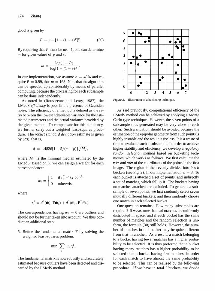
Figure 2. Illustration of a bucketing technique.

As said previously, computational efficiency of theLMedS method can be achieved by applying a MonteCarlo type technique. However, the seven points of asubsample thus generated may be very close to eachother. Such a situation should be avoided because theestimation of the epipolar geometry from such points ishighly instable and the result is useless. It is a waste oftime to evaluate such a subsample. In order to achievehigher stability and efficiency, we develop aregularlyrandom selection methodbased on bucketing tech-niques, which works as follows. We first calculate themin andmax of the coordinates of the points in the firstimage. The region is then evenly divided intob× bbuckets (see Fig. 2). In our implementation,b = 8. Toeach bucket is attached a set of points, and indirectlya set of matches, which fall in it. The buckets havingno matches attached are excluded. To generate a sub-sample of seven points, we first randomly select sevenmutually different buckets, and then randomly chooseone match in each selected bucket.

One question remains: How many subsamples arerequired? If we assume that bad matches are uniformlydistributed in space, and if each bucket has the samenumber of matches and the random selection is uni-form, the formula (30) still holds. However, the num-ber of matches in one bucket may be quite differentfrom that in another. As a result, a match belongingto a bucket having fewer matches has a higher proba-bility to be selected. It is thus preferred that a buckethaving many matches has a higher probability to beselected than a bucket having few matches, in orderfor each match to have almost the same probabilityto be selected. This can be realized by the followingprocedure. If we have in totall buckets, we divide

P1: NTA



Figure 3. Interval and bucket mapping.

range [0 1] intol intervals such that the width of thei th interval is equal toni /

∑i ni , whereni is the num-

ber of matches attached to thei th bucket (see Fig. 3).During the bucket selection procedure, a number, pro-duced by a [0 1] uniform random generator, falling inthe i th interval implies that thei th bucket is selected.

Together with the matching technique describedin (Zhang et al., 1995), we have implemented this ro-bust method and successfully solved, in an automaticway, the matching and epipolar geometry recoveryproblem for different types of scenes such as indoor,rocks, road, and textured dummy scenes. The corre-sponding softwareimage-matching has been madeavailable on the Internet since 1994.

3.8. Characterizing the Uncertaintyof Fundamental Matrix

Since the data points are always corrupted by noise,and sometimes the matches are even spurious or incor-rect, one should model the uncertainty of the estimatedfundamental matrix in order to exploit its underlyinggeometric information correctly and effectively. Forexample, one can use the covariance of the fundamentalmatrix to compute the uncertainty of the projectivereconstruction or the projective invariants, or to im-prove the results of Kruppa’s equation for a better self-calibration of a camera (Zeller, 1996).

In order to quantify the uncertainty related to theestimation of the fundamental matrix by the methoddescribed in the previous sections, we model the fun-damental matrix as a random vectorf ∈ IR7 (vectorspace of real 7-vectors) whose mean is the exact valuewe are looking for. Each estimation is then considered

as a sample off and the uncertainty is given by thecovariance matrix off.

In the remaining of this subsection, we consider ageneral random vectory ∈ IRp, wherep is the dimen-sion of the vector space. The same discussion applies,of course, directly to the fundamental matrix. Thecovariance ofy is defined by the positive symmetricmatrix

Λy = E[(y− E[y])(y− E[y])T ], (31)

whereE[y] denotes the mean of the random vectory.

3.8.1. The Statistical Method. The statistical methodconsists in using the well-known large number law toapproximate the mean: if we have a sufficiently largenumberN of samplesyi of a random vectory, thenE[y] can be approximated by the sample mean

EN [yi ] = 1

N

N∑i=1

yi ,

andΛy is then approximated by

1

N − 1

N∑i=1

[(yi − EN [yi ])(yi − EN [yi ])T ]. (32)

A rule of thumb is that this method works reasonablewell whenN > 30. It is especially useful for simula-tion. For example, through simulation, we have foundthat the covariance of the fundamental matrix estimatedby the analytical method through a first order approxi-mation (see below) is quite good when the noise levelin data points is moderate (the standard deviation is notlarger than one pixel) (Csurka et al., 1996).

3.8.2. The Analytical Method

The Explicit Case. We now consider the case thaty iscomputed from another random vectorx of IRm usingaC1 functionϕ:

y = ϕ(x).

Writing the first order Taylor expansion ofϕ in theneighborhood ofE[x] yields

ϕ(x) = ϕ(E[x])+ Dϕ(E[x]) · (x− E[x])

+O(x− E[x])2, (33)

P1: NTA


176 Zhang

where O(x)2 denotes the terms of order 2 or higherin x, andDϕ(x) = ∂ϕ(x)/∂x is the Jacobian matrix.Assuming that any sample ofx is sufficiently close toE[x], we can approximateϕ by the first order terms of(33) which yields:

E[y] ' ϕ(E[x]),

ϕ(x)−ϕ(E[x]) ' Dϕ(E[x]) · (x− E[x]).

The first order approximation of the covariance matrixof y is then given in function of the covariance matrixof x by

Λy = E[(ϕ(x)−ϕ(E[x]))(ϕ(x)−ϕ(E[x]))T ]

= Dϕ(E[x])ΛxDϕ(E[x])T . (34)

The Case of an Implicit Function.In some cases likeours, the parameter is obtained through minimization.Therefore,ϕ is implicit and we have to make use ofthe well-known implicit functions theorem to obtainthe following result (see Faugeras, 1993; Chap. 6).

Proposition 1. Let a criterion function C: IRm ×IRp → IR be a function of class C∞, x0 ∈ IRm bethe measurement vector andy0 ∈ IRp be a local mini-mum of C(x0, z). If the HessianH of C with respect toz is invertible at(x, z) = (x0, y0) then there exists anopen set U′ of IRm containingx0 and an open set U′′

of IRpcontainingy0 and a C∞ mappingϕ: IRm→ IRp

such that for(x, y) in U ′ × U ′′ the two relations“yis a local minimum of C(x, z) with respect toz” andy = ϕ(x) are equivalent. Furthermore, we have thefollowing equation:

Dϕ(x) = −H−1∂Φ∂x, (35)

where

Φ =(∂C

∂z

)T

and H = ∂Φ∂z.

Taking x0 = E[x] and y0 = E[y], Eq. (34) thenbecomes

Λy = H−1∂Φ∂x

Λx

(∂Φ∂x

)T

H−T . (36)

The Case of a Sum of Squares of Implicit Functions.Here we study the case whereC is of the form:

n∑i=1

C2i (xi , z)

with x = [xT1 , . . . , x

Ti , . . . , x

Tn ]T . Then, we have

Φ = 2∑

i

Ci

(∂Ci

∂z

)T

H = ∂Φ∂z= 2

∑i

(∂Ci

∂z

)T∂Ci

∂z+ 2

∑i

Ci∂2Ci

∂z2.

Now, it is a usual practice to neglect the termsCi∂2Ci∂z2

with respect to the terms( ∂Ci∂z )

T ∂Ci∂z (see classical books

of numerical analysis (Press et al., 1988)) and the nu-merical tests we did confirm that we can do this becausethe former is much smaller than the latter. We can thenwrite:

H = ∂Φ∂z≈ 2

∑i

(∂Ci

∂z

)T∂Ci

∂z.

In the same way we have:

∂Φ∂x≈ 2

∑i

(∂Ci

∂z

)T∂Ci

∂x.

Therefore, Eq. (36) becomes:

Λy = 4H−1∑i, j

(∂Ci∂z

)T∂Ci∂x Λx

(∂Cj

∂x

)T∂Cj

∂z H−T .

(37)

Assume that the noise inxi and that inx j ( j 6= i )are independent (which is quite reasonable becausethe points are extracted independently), thenΛxi, j =E[(xi − xi )(x j − x j )

T ] = 0 andΛx = diag(Λx1, . . . ,

Λxn). Equation (37) can then be written as

Λy = 4H−1∑

i

(∂Ci

∂z

)T∂Ci

∂xiΛxi

(∂Ci

∂xi

)T∂Ci

∂zH−T .

SinceΛCi = ∂Ci∂xi

Λxi (∂Ci∂xi)T by definition (up to the first

order approximation), the above equation reduces to

Λy = 4H−1∑

i

(∂Ci

∂z

)T

ΛCi

∂Ci

∂zH−T . (38)

P1: NTA



Considering that the mean of the value ofCi at theminimum is zero and under the somewhat strong as-sumption that theCi ’s are independent and have identi-cal distributed errors (Note: it is under this assumptionthat the solution given by the least-squares technique isoptimal), we can then approximateΛCi by its samplevariance (see e.g., Anderson, 1958):

ΛCi =1

n− p

∑i

C2i =

S

n− p,

whereS is the value of the criterionC at the minimum,andp is the number of parameters, i.e., the dimensionof y. Although it has little influence whenn is big, theinclusion of p in the formula above aims at correctingthe effect of a small sample set. Indeed, forn = p,we can almost always find an estimate ofy such thatCi = 0 for all i , and it is not meaningful to estimatethe variance. Equation (38) finally becomes

Λy = 2S

n− pH−1HH−T = 2S

n− pH−T . (39)

The Case of the Fundamental Matrix.As explainedin Section 3.4,F is computed using a sum of squares ofimplicit functions ofn point correspondences. Thus,referring to the previous paragraph, we havep = 7,and the criterion functionC(m, f7) (wherem = [m1,

m′1, . . . ,mn,m′n]T and f7 is the vector of the sevenchosen parameters forF) is given by (15).Λf7 is thuscomputed by (39) using the Hessian obtained as a by-product of the minimization ofC(m, f7).

According to (34),ΛF is then computed fromΛf7:

ΛF = ∂F(f7)

∂f7Λf7

∂F(f7)

∂f7

T

. (40)

Here, we actually consider the fundamental matrixF(f7) as a 9-vector composed of the nine coefficientswhich are functions of the seven parametersf7.

The reader is referred to (Zhang and Faugeras, 1992,Chap. 2) for a more detailed exposition on uncertaintymanipulation.

3.9. Other Techniques

To close the review section, we present two analyt-ical techniques and one robust technique based onRANSAC.

3.9.1. Virtual Parallax Method. If two sets of im-age points are the projections of a plane in space (seeSection 5.2), then they are related by a homographyH. For points not on the plane, they do not verify thehomography, i.e.,m′ 6= ρHm, whereρ is an arbitrarynon-zero scalar. The difference (i.e., parallax) allowsus to estimate directly an epipole if the knowledge ofH is available. Indeed, Luong and Faugeras (1996)show that the fundamental matrix and the homographyis related byF = [e′]×H. For a point which does notbelong to the plane,l′ = m′ × Hm defines an epipo-lar line, which provides one constraint on the epipole:e′T l′ = 0. Therefore, two such points are sufficient toestimate the epipolee′. The generate-and-test methods(see e.g., Faugeras and Lustman, 1988), can be used todetect the coplanar points.

The virtual parallax method proposed by Boufamaand Mohr (1995) does not require the prior identifica-tion of a plane. To simplify the computations, withoutloss of generality, we can perform a change of projec-tive coordinates in each image such that

m1= [1, 0, 0]T , m2= [0, 1, 0]T , m3= [0, 0, 1]T ,

m4= [1, 1, 1]T ; (41)

m′1= [1, 0, 0]T , m′2= [0, 1, 0]T , m′3= [0, 0, 1]T ,

m′4 = [1, 1, 1]T . (42)

These points are chosen such that no three of them arecollinear. The three first points define a plane in space.Under such choice of coordinate systems, the homogra-phy matrix such thatm′i = ρHmi (i = 1, 2, 3) is diag-onal, i.e.,H = diag(a, b, c), and depends only on twoparameters. Let the epipole bee′ = [e′u, e

′v, e′t ]

T . As wehave seen in the last paragraph, for each additional point(mi ,m′i ) (i = 4, . . . ,n), we havee′T (m′i × Hmi ) = 0,i.e.,

v′i e′uc− vi e

′ub+ ui e

′va− u′i e

′vc+ u′i vi e

′t b

−v′i ui e′ta = 0. (43)

This is the basic epipolar equation based on virtual par-allax. Since(a, b, c) and(e′u, e

′v, e′t ) are defined each

up to a scale factor, the above equation is polynomial ofdegree two in four unknowns. To simplify the problem,we make the following reparameterization. Let

x1 = e′uc, x2 = e′ub, x3 = e′va,x4 = e′vc, x5 = e′t b, and x6 = e′ta,

P1: NTA


178 Zhang

which are defined up to a common scale factor. Equa-tion (43) now becomes

v′i x1− vi x2+ ui x3− u′i x4+ u′i vi x5− v′i ui x6 = 0.

(44)

Unlike (43), we here have five independent variables,one more than necessary. The unknownsxi (i =1, . . . ,6) can be solved linearly if we have five or morepoint matches. Thus, we need in total eight point cor-respondences, like the eight-point algorithm. The orig-inal unknowns can be computed, for example, as

e′u = e′t x2/x5, e′v = e′t x3/x6,

a = cx3/x4, b = cx2/x1.(45)

The fundamental matrix is finally obtained as[e′]× diag(a, b, c), and the rank constraint is automat-ically satisfied. However, note that

• the computation (45) is not optimal, because eachintermediate variablexi is not used equally;• the rank-2 constraint in the linear Eq. (44) is not

necessarily satisfied because of the introduction ofan intermediate parameter.

Therefore, the rank-2 constraint is also imposed aposteriori, similar to the eight-point algorithm (seeSection 3.2).

The results obtained with this method depends on thechoice of the four basis points. The authors indicatethat a good choice is to take them largely spread in theimage.

Experiments show that this method produces goodresults. Factors which contribute to this are the factthe dimensionality of the problem has been reduced,and the fact that the change of projective coordinatesachieve a data renormalization comparable to the onedescribed in Section 3.2.5.

3.9.2. Linear Subspace Method.Ponce and Genc(1996), through a change of projective coordinates, setup a set of linear constraints on one epipole using thelinear subspace method proposed by Heeger and Jepson(1992). A change of projective coordinates in each im-age as described in (41) and (42) is performed. Further-more, we choose the corresponding four scene pointsMi (i = 1, . . . ,4) and the optical center of each cameraas a projective basis in space. We assign to the basis

points for the first camera the following coordinates:

M1 = [1, 0, 0, 0]T , M2 = [0, 1, 0, 0]T ,

C = [0, 0, 1, 0]T , (46)

M3 = [0, 0, 0, 1]T , M4 = [1, 1, 1, 1]T .

The same coordinates are assigned to the basis pointsfor the second camera. Therefore, the camera projec-tion matrix for the first camera is given by

P=

1 0 0 0

0 1 0 0

0 0 0 1

. (47)

Let the coordinates of the optical centerC of the firstcamera be [α, β, γ,1]T in the projective basis of thesecond camera, and let the coordinates of the four scenepoints remain the same in both projective bases, i.e.,M′i = Mi (i = 1, . . . ,4). Then, the coordinate transfor-mationH from the projective basis of the first camerato that of the second camera is given by

H =

γ − α 0 α 0

0 γ − β β 0

0 0 γ 0

0 0 1 γ − 1

. (48)

It is then a straightforward manner to obtain the pro-jection matrix of the first camera with respect to theprojective basis of the second camera:

P′ = PH =

γ − α 0 α 0

0 γ − β β 0

0 0 1 γ − 1

. (49)

According to (6), the epipolar equation ism′Ti Fmi

= 0, while the fundamental matrix is given byF= [P′p⊥]×P′P+. Since

p⊥ = C =

0

0

1

0

P+ = PT (PPT )−1 =

1 0 0

0 1 0

0 0 0

0 0 1

,

P1: NTA



we obtain the fundamental matrix:

F = [e′]× diag(γ − α, γ − β, γ − 1), (50)

wheree′ ≡ P′p⊥ = [α, β,1]T is just the projection ofthe first optical center in the second camera, i.e., thesecond epipole.

Consider now the remaining point matches{(mi ,m′i ) | i = 5, . . . ,n}, wheremi = [ui , vi , 1]T

andm′i = [u′i , v′i , 1]T . From (50), after some simple

algebraic manipulation, the epipolar equation can berewritten as

γgTi e′ = qT

i f,

wheref = [α, β, αβ]T , gi = m′i × mi = [v′i − vi , ui −u′i ,−v′i ui + u′i vi ]T and qi = [v′i (1 − ui ),−u′i (1 −vi ), ui − vi ]T . Consider a linear combination of theabove equations. Let us define the coefficient vectorξ = [ξ5, . . . , ξn]T and the vectorsτ (ξ) = ∑n

i=5 ξi gi

andχ(ξ) =∑ni=5 ξi qi . It follows that

γ τ (ξ)T e′ = χ(ξ)T f. (51)

The idea of the linear subspace is that for any valueξτsuch thatτ (ξτ )= 0, Eq. (51) provides a linear con-straint onf, i.e., χ(ξτ )

T f = 0, while for any valueξχ such thatχ(ξχ)= 0, the same equation providesa linear constraint one′, i.e., τ (ξχ)

T e′ = 0. Becauseof the particular structure ofgi and qi , it is easyto show (Ponce and Genc, 1996) that the vectorsτ (ξχ) andχ(ξτ ) are both orthogonal to the vector[1, 1, 1]T . Since the vectorsτ (ξχ) are also orthogonalto e′, they only span a one-dimensional line, and theirrepresentative vector is denoted byτ 0 = [aτ , bτ , cτ ]T .Likewise, the vectorsχ(ξτ ) span a line orthogonal toboth f and [1, 1, 1]T , and their representative vector isdenoted byχ0 = [aχ , bχ , cχ ]T . Assume for the mo-ment that we knowτ 0 andχ0 (their computation will bedescribed shortly), from [aτ , bτ ,−aτ −bτ ]T e′ = 0 and[aχ , bχ ,−aχ − bχ ]T f = 0, the solution to the epipoleis given by

α = bχaτ

aτ + bτaχ + bχ

, β = aχbτ

aτ + bτaχ + bχ

. (52)

Once the epipole has been computed, the remainingparameters of the fundamental matrix can be easilycomputed.

We now turn to the estimation ofτ 0 andχ0. Fromthe above discussion, we see that the set of linear com-binations

∑ni=5 ξgi such that

∑ni=5 ξqi = 0 is one-

dimensional. Construct two 3× (n− 4) matrices:

G = [g5, . . . ,gn] and Q = [q5, . . . ,qn].

The set of vectorsξ such that∑n

i=5 ξqi = 0 is simplythe null space ofQ. Let Q = U1S1VT

1 be the singularvalue decomposition (SVD) ofQ, then the null spaceis formed by the rightmostn− 4− 3= n− 7 columnsof V1, which will be denoted byV0. Then, the set ofvectors

∑ni=5 ξgi such that

∑ni=5 ξqi = 0 is thus the

subspace spanned by the matrixGV0, which is 3×(n− 7). Let GV0 = U2S2VT

2 be the SVD. Accordingto our assumptions, this matrix has rank 1, thusτ 0 istherangeof GV0, which is simply the leftmost columnof U2 up to a scale factor. Vectorχ0 can be computedfollowing the same construction by reversing the rˆolesof τ andχ.

The results obtained with this method depends onthe choice of the four basis points. The authors showexperimentally that a good result can be obtained bytrying 30 random basis choices and picking up the so-lution resulting the smallest epipolar distance error.

Note that although unlike the virtual parallaxmethod, the linear subspace technique provides a lin-ear algorithm without introducing an extraneous pa-rameter, it is achieved in (52) by simply dropping theestimated information incτ andcχ . In the presenceof noise,τ 0 andχ0 computed through singular valuedecomposition do not necessarily satisfyτ T

0 1= 0 andχT

0 1= 0, where1= [1, 1, 1]T .Experiments show that this method produces good

results. The same reasons as for the virtual parallaxmethod can be used here.

3.9.3. RANSAC. Random sample consensus(RANSAC) (Fischler and Bolles, 1981) is a paradigmoriginated in the Computer Vision community for ro-bust parameter estimation. The idea is to find, throughrandom sampling of a minimal subset of data, the pa-rameter set which is consistent with a subset of dataas large as possible. The consistent check requires theuser to supply a threshold on the errors, which reflectsthe a priori knowledge of the precision of the expectedestimation. This technique is used by Torr (1995) to es-timate the fundamental matrix. As is clear, RANSACis very similar to LMedS both in ideas and in imple-mentation, except that

P1: NTA


180 Zhang

• RANSAC needs a threshold to be set by the user forconsistence checking, while the threshold is auto-matically computed in LMedS;• In step 3 of the LMedS implementation described in

Section 3.7.2, the size of the point matches whichare consistent withFJ is computed, instead of themedian of the squared residuals.

However, LMedS cannot deal with the case wherethe percentage of outliers is higher than 50%, whileRANSAC can. Torr and Murray (1993) compared bothLMedS and RANSAC. RANSAC is usually cheaperbecause it can exit the random sampling loop once aconsistent solution is found.

If one knows that the number of outliers is more than50%, then they can easily adapt the LMedS by usingan appropriate value, say 40%, instead of using the me-dian. (When we do this, however, the solution obtainedmay be notglobally optimal if the number of outliersis less than 50%.) If there is a large set of images ofthe same type of scenes to be processed, one can firstapply LMedS to one pair of the images in order to findan appropriate threshold, and then apply RANSAC tothe remaining images because it is cheaper.

4. An Example of Fundamental MatrixEstimation with Comparison

The pair of images is a pair of calibrated stereo images(see Fig. 4). By “calibrated” is meant that the intrin-sic parameters of both cameras and the displacement

Figure 4. Image pair used for comparing different estimation techniques of the fundamental matrix.

between them were computed off-line through stereocalibration. There are 241 point matches, which areestablished automatically by the technique describedin (Zhang et al., 1995). Outliers have been discarded.The calibrated parameters of the cameras are of coursenot used, but the fundamental matrix computed fromthese parameters serves as a ground truth. This is shownin Fig. 5, where the four epipolar lines are displayed,corresponding, from the left to the right, to the pointmatches 1, 220, 0 and 183, respectively. The intersec-tion of these lines is the epipole, which is clearly veryfar from the image. This is because the two camerasare placed almost in the same plane.

The epipolar geometry estimated with the linearmethod is shown in Fig. 6 for the same set of pointmatches. One can find that the epipole is now in theimage, which is completely different from what wehave seen with the calibrated result. If we perform adata normalization before applying the linear method,the result is considerably improved, as shown in Fig. 7.This is very close to the calibrated one.

The nonlinear method gives even better result, asshown in Fig. 8. A comparison with the “true” epipo-lar geometry is shown in Fig. 9. There is only a smalldifference in the orientation of the epipolar lines. Wehave also tried the normalization method followed bythe nonlinear method, and the same result was obtained.Other methods have also been tested, and visually al-most no difference is observed.

Quantitative results are provided in Table 1, wherethe elements in the first column indicates the meth-ods used in estimating the fundamental matrix:

P1: NTA



Figure 5. Epipolar geometry estimated through classical stereo calibration, which serves as the ground truth.

Figure 6. Epipolar geometry estimated with the linear method.

they are respectively the classical stereo calibra-tion (Calib.), the linear method with eigen analysis(linear), the linear method with prior data normaliza-tion (normal.), the nonlinear method based on mini-mization of distances between points and epipolar lines(nonlinear), the nonlinear method based on minimiza-tion of gradient-weighted epipolar errors (gradient),the M-estimator with Tukey function (M-estim.),the nonlinear method based on minimization of dis-tances between observed points and reprojected ones

(reproj. ), and the LMedS technique (LMedS). Thefundamental matrix ofCalib is used as a reference.The second column shows the difference between thefundamental matrix estimated by each method with thatof Calib. The difference is measured as the Frobeniusnorm:1F = ‖F−FCalib‖×100%. Since eachF is nor-malized by its Frobenius norm,1F is directly related tothe angle between two unit vectors. It can be seen thatalthough we have observed that Methodnormal hasconsiderably improved the result of the linear method,

P1: NTA


182 Zhang

Figure 7. Epipolar geometry estimated with the linear method with prior data normalization.

Figure 8. Epipolar geometry estimated with the nonlinear method.

its1F is the largest. It seems that1F is not appropri-ate to measure the difference between two fundamentalmatrix. We will describe another one in the next para-graph. The third and fourth columns show the positionsof the two epipoles. The fifth column gives the root ofthe mean of squared distances between points and theirepipolar lines. We can see that even withCalib, theRMS is as high as 1 pixel. There are two possibilities:either the stereo system is not very well calibrated, or

the points are not well localized; and we think the latteris the major reason because the corner detector we useonly extracts points within pixel precision. The lastcolumn shows the approximate CPU time in secondswhen the program is run on a Sparc 20 workstation.Nonlinear, gradient and reproj give essentially thesame result (but the latter is much more time consum-ing). The M-estimator and LMedS techniques give thebest results. This is because the influence of poorly

P1: NTA



Figure 9. Comparison between the Epipolar geometry estimated through classical stereo calibration (shown in Red/Dark lines) and thatestimated with the nonlinear method (shown in Green/Grey lines).

Figure 12. Epipolar bands for several point matches.

P1: NTA


184 Zhang

Table 1. Comparison of different methods for estimating the fundamental matrix.

Method 1F e e′ RMS CPU

Calib. 5138.18 −8875.85 1642.02 −2528.91 0.99

Linear 5.85% 304.018 124.039 256.219 230.306 3.40 0.13 s

Normal. 7.20% −3920.6 7678.71 8489.07 −15393.5 0.89 0.15 s

Nonlinear 0.92% 8135.03 −14048.3 1896.19 −2917.11 0.87 0.38 s

Gradient 0.92% 8166.05 −14104.1 1897.80 −2920.12 0.87 0.40 s

M-estim. 0.12% 4528.94 −7516.3 1581.19 −2313.72 0.87 1.05 s

Reproj. 0.92% 8165.05 −14102.3 1897.74 −2920.01 0.87 19.1 s

LMedS 0.13% 3919.12 −6413.1 1500.21 −2159.65 0.75 2.40 s

localized points has been reduced in M-estimator orthey are simply discarded in LMedS. Actually, LMedShas detected five matches as outliers, which are 226,94, 17, 78 and 100. Of course, these two methods aremore time consuming than the nonlinear method.

4.1. A Measure of Comparison BetweenFundamental Matrices

From the above discussion, the Frobenius norm of thedifference between two normalized fundamental ma-trices is clearly not an appropriate measure of compar-ison. In the following, we describe a measure proposedby Stephane Laveau from INRIA Sophia-Antipolis,which we think characterizes well the difference be-tween two fundamental matrices. Let the two givenfundamental matrices beF1 andF2. The measure iscomputed as follows (see Fig. 10):

Step 1: Chooserandomly a point m in the firstimage.

Step 2: Draw the epipolar line ofm in the second imageusingF1. The line is shown as a dashed line, and isdefined byF1m.

Figure 10. Definition of the difference between two fundamentalmatrices in terms of image distances.

Step 3: If the epipolar line does not intersect the secondimage, go to Step 1.

Step 4: Chooserandomlya pointm′ on the epipolarline. Note thatm andm′ correspond to each otherexactly with respect toF1.

Step 5: Draw the epipolar line ofm in the second imageusingF2, i.e.,F2m, and compute the distance, notedby d′1, between pointm′ and lineF2m.

Step 6: Draw the epipolar line ofm′ in the first imageusingF2, i.e.,FT

2 m′, and compute the distance, notedby d1, between pointm and lineFT

2 m′.Step 7: Conduct the same procedure from Step 2

through Step 6, but reversing the roles ofF1 andF2,and computed2 andd′2.

Step 8: RepeatN times Step 1 through Step 7.Step 9: Compute the average distance ofd’s, which

is the measure of difference between the two funda-mental matrices.

In this procedure, a random number generator basedon uniform distribution is used. The two fundamen-tal matrices plays a symmetric role. The two imagesplays a symmetric role too, although it is not at firstsight. The reason is thatm and m′ are chosen ran-domly and the epipolar lines are symmetric (lineFT

1 m′

goes throughm). Clearly, the measure computed asabove,in pixels, is physically meaningful, because itis defined in the image space in which we observe thesurrounding environment. Furthermore, whenN tendsto infinity, we sample uniformly the whole 3D spacevisible from the given epipolar geometry. If the imageresolution is 512×512 and if we consider a pixel reso-lution, then the visible 3D space can be approximatelysampled by 5123 points. In our experiment, we setN = 50000. Using this method, we can compute thedistance between each pair of fundamental matrices,and we obtain a symmetric matrix.

P1: NTA



Table 2. Distances between the fundamental matrices estimated by different techniques

Linear Normal. Nonlinear Gradient M-estim. Reproj. LMedS

Calib. 116.4 5.97 2.66 2.66 2.27 2.66 1.33

Linear 117.29 115.97 116.40 115.51 116.25 115.91

Normal. 4.13 4.12 5.27 4.11 5.89

Nonlinear 0.01 1.19 0.01 1.86

Gradient 1.19 0.00 1.86

M-estim. 1.20 1.03

Reproj. 1.88

The result is shown in Table 2, where only the uppertriangle is displayed (because of symmetry). We arriveat the following conclusions:

• The linear method is very bad.• The linear method with prior data normalization

gives quite a reasonable result.• The nonlinear method based on point-line distances

and that based on gradient-weighted epipolar errorsgive very similar results to those obtained based onminimization of distances between observed pointsand reprojected ones. The latter should be avoidedbecause it is too time consuming.• M-estimators or the LMedS method give still better

results because they try to limit or eliminate the effectof poorly localized points. The epipolar geometryestimated by LMedS is closer to the one computedthrough stereo calibration.

The LMedS method should be definitely used if thegiven set of matches contain false matches.

4.2. Epipolar Band

Due to space limitation, the result on the uncertaintyof the fundamental matrix is not shown here, and canbe found in (Csurka et al., 1996), together with its usein computing the uncertainty of the projective recon-struction and in improving the self-calibration basedon Kruppa equations. We show in this section howto use the uncertainty to define the epipolar band formatching.

We only consider the epipolar lines in the secondimage (the same can be done for the first). For a givenpoint m0 = [u0, v0]T in the first image together withits covariance matrixΛm0 = [ σuu σuv

σuv σvv], its epipolar line

in the second image is given byl′0 = Fm0. From (34),

the covariance matrix ofl′ is computed by

Λl′0 =∂ l′0∂F

ΛF

(∂ l′0∂F

)T

+ F

[Λm0 02

0T2 0

]FT , (53)

whereF in the first term of the right hand is treated asa 9-vector, and02 = [0, 0]T .

Any point m′ = [u′, v′]T on the epipolar linel′0 ≡[l ′1, l

′2, l′3]T must satisfym′T l′0 = l′T0 m′ = l ′1u′ + l ′2v

′ +l ′3 = 0 (we see theduality between points and lines).The vectorl′0 is defined up to a scale factor. It is a pro-jective point in the dual space of the image plane, andis the dual of the epipolar line. We consider the vectorof parametersx0 = (x0, y0) = (l ′1/l ′3, l ′2/l ′3)T (if l ′3 = 0we can choose(l ′1/l

′2, l′3/l′2) or (l ′2/l

′1, l′3/l′1)). The co-

variance matrix ofx0 is computed in the same way as(34): C = (∂ l′0/∂x0)Λl′0(∂ l′0/∂x0)

T . The uncertaintyof x0 can be represented in the usual way by an ellipseC in the dual space (denoted byx) of the image plane:

(x− x0)TC−1(x− x0) = k2, (54)

wherek is a confidence factor determined by theχ2 dis-tribution of 2 degrees of freedom. The probability thatx appears at the interior of the ellipse defined by (54)is equal toPχ2(k, 2). Equation (54) can be rewritten inprojective form as

xTAx = 0 with A =[

C−1 −C−1x0

−xT0 C−T xT

0 C−1x0− k2

].

The dual of this ellipse, denoted byC∗, defines aconic in the image plane. It is given by

mTA∗m = 0 (55)

where A∗ is the adjoint of matrixA (i.e., A∗A =det(A) I ). Because of the duality between the param-eter spacex and the image planem (see Fig. 11),for a point x on C, it defines an epipolar line in the

P1: NTA


186 Zhang

Figure 11. Duality between the image plane and the parameterspace of the epipolar lines.

image plane, line(x), which is tangent to conicC∗ at apointm, while the latter defines a line in the parameterspace, line(m), which is tangent toC at x. It can beshown (Csurka, 1996) that, for a point in the interior ofellipseC, the corresponding epipolar line lies outsideof conicC∗ (i.e., it does not cut the conic). Therefore,for a givenk, the outside of this conic defines the regionin which the epipolar line should lie with probabilityPχ2(k, 2). We call this region theepipolar band. For agiven point in one image, its match should be searchedin this region. Although, theoretically, the uncertaintyconic defining the epipolar band could be an ellipse orparabola, it is always an hyperbola in practice (exceptwhenΛF is extremely huge).

We have estimated the uncertainty of the funda-mental matrix for the image pair shown in Fig. 4. InFig. 12, we show the epipolar bands of matches 1, 220,0 and 183 in the second images, computed as describedabove. The displayed hyperbolas correspond to a prob-ability of 70% (k = 2.41) with image point uncertaintyof σuu = σvv = 0.52 and σuv = 0. We have alsoshown in Fig. 12 the epipolar lines drawn in dashedlines and the matched points indicated in+. An inter-esting thing is that the matched points are located in thearea where the two sections of hyperbolas are closestto each other. This suggests that the covariance matrixof the fundamental matrix actually captures, to someextent, the matching information (disparity in stereoterminology). Such areas should be first examined insearching for point matches. This may, however, notbe true if a significant depth discontinuity presents inthe scene and if the point matches used in computingthe fundamental matrix do not represent sufficientlyenough the depth variation.

5. Discussion

In this paper, we have reviewed a number of techniquesfor estimating the epipolar geometry between two im-ages. Point matches are assumed to be given, but some

of them may have been incorrectly paired. How to es-tablish point matches is the topic of the paper (Zhanget al., 1995).

5.1. Summary

For two uncalibrated images under full perspective pro-jection, at least seven point matches are necessary todetermine the epipolar geometry. When only sevenmatches are available, there are possibly three solu-tions, which can be obtained by solving a cubic equa-tion. If more data are available, then the solution is ingeneral unique and several linear techniques have beendeveloped. The linear techniques are usually sensitiveto noise and not very stable, because they ignore theconstraints on the nine coefficients of the fundamen-tal matrix and the criterion they are minimizing is notphysically meaningful. The results, however, can beconsiderably improved by first normalizing the datapoints, instead of using pixel coordinates directly, suchthat their new coordinates are on the average equal tounity. Even better results can be obtained under non-linear optimization framework by

• using an appropriate parameterization of fundamen-tal matrix to take into account explicitly the rank-2constraint, and• minimizing a physically meaningful criterion.

Three choices are available for the latter: the distancesbetween points and their corresponding epipolar lines,the gradient-weighted epipolar errors, and the distancesbetween points and the reprojections of their corre-sponding points reconstructed in space. Experimentsshow that the results given by the optimization basedon the first criterion are slightly worse than the last twowhich give essentially the same results. However, thethird is much more time consuming, and is thereforenot recommended, although it is statistically optimalunder certain conditions. One can, however, use itas the last step to refine the results obtained with thefirst or second technique. To summarize, we recom-mend the second criterion (gradient-weighted epipolarerrors), which is actually a very good approximation tothe third one.

Point matches are obtained by using some heuristictechniques such as correlation and relaxation, and theyusually contain false matches. Also, due to the lim-ited performance of a corner detector or low contrastof an image, a few points are possibly poorly local-ized. These outliers (sometimes even one) will severelyaffect the precision of the fundamental matrix if we

P1: NTA



directly apply the methods described above, whichare all least-squares techniques. We have thus pre-sented in detail two commonly used robust techniques:M-Estimators and Least Median of Squares (LMedS).M-estimators try to reduce the effect of outliers byreplacing the squared residuals by another functionof the residuals which is less increasing than square.They can be implemented as an iterated reweightedleast-squares. Experiments show that they are robustto outliers due to bad localization, but not robust tofalse matches. This is because they depend tightly onthe initial estimation of the fundamental matrix. TheLMedS method solves a nonlinear minimization prob-lem which yields the smallest value for the median ofsquared residuals computed for the entire data set. Itturns out that this method is very robust to false matchesas well as to outliers due to bad localization. Unfor-tunately, there is no straightforward formula for theLMedS estimator. It must be solved by a search in thespace of possible estimates generated from the data.Since this space is too large, only a randomly chosensubset of data can be analyzed. We have proposeda regularly random selection method to improve theefficiency.

Since the data points are always corrupted by noise,one should model the uncertainty of the estimated fun-damental matrix in order to exploit its underlying geo-metric information correctly and effectively. We havemodeled the fundamental matrix as a random vectorin its parameterization space and described methods toestimate the covariance matrix of this vector under thefirst order approximation. This uncertainty measurecan be used to define the epipolar band for matching,as shown in Section 4.2. In (Csurka et al., 1996), wealso show how it can be used to compute the uncer-tainty of the projective reconstruction and to improvethe self-calibration based on Kruppa equations.

Techniques for projective reconstruction will be re-viewed in Appendix A. Although we cannot obtainany metric information from a projective structure(measurements of lengths and angles do not makesense), it still contains rich information, such as copla-narity, collinearity, and ratios, which is sometimes suf-ficient for artificial systems, such as robots, to performtasks such as navigation and object recognition.

5.2. Degenerate Configurations

Up to now, we have only considered the situationswhere no ambiguity arises in interpreting a set of pointmatches (i.e., they determine a unique fundamental

matrix), except for the case of seven point matcheswhere three solutions may exist. Sometimes, however,even with a large set of point matches, there exist manysolutions for the fundamental matrix which explain thedata equally well, and we call such situations degener-ate for the determination of the fundamental matrix.

Maybank (1992) has thoroughly studied the degen-erate configurations:

• 3D points lie on a quadric surface passing throughthe two optical centers (called the critical surface,or maybank quadricby Longuet-Higgins). We mayhave three different fundamental matrices compati-ble with the data. The two sets of image points arerelated by a quadratic transformation:

m′ = F1m× F2m,

whereF1 andF2 are two of the fundamental matrices.• The two sets of image points are related by a homog-

raphy:

m′ = ρHm,

whereρ is an arbitrary non-zero scalar, andH is a3× 3 matrix defined up to a scale factor. This is adegenerate case of the previous situation. It ariseswhen 3D points lie on a plane or when the cameraundergoes a pure rotation around the optical center(equivalent to the case when all points lie on a planeat infinity).• 3D points are in even more special position, for ex-

ample on a line.

The stability of the fundamental matrix related to thedegenerate configurations is analyzed in (Luong andFaugeras, 1996). A technique which automatically de-tects the degeneracy based onχ2 test when the noiselevel of the data points is known is reported in (Torret al., 1995, 1996).

5.3. Affine Cameras

So far, we have only considered images under perspec-tive projection, which is a nonlinear mapping from3D space to 2D. This makes many vision problemsdifficult to solve, and more importantly, they can be-come ill-conditioned when the perspective effects aresmall. Sometimes, if certain conditions are satisfied,for example, when the camera field of view is smalland the object size is small enough with respect to the

P1: NTA


188 Zhang

distance from the camera to the object, the projectioncan be approximated by a linear mapping (Aloimonos,1990). The affine camera introduced in (Mundy andZisserman, 1992) is a generation of the orthographicand weak perspective models. Its projection matrix hasthe following special form:

PA =

P11 P12 P13 P14

P21 P22 P23 P24

0 0 0 P34

defined up to a scale factor. The epipolar constraint (5)is still valid, but the fundamental matrix (6) will be ofthe following simple form (Xu and Zhang, 1996):

FA =

0 0 a13

0 0 a23

a31 a32 a33

.This is known as theaffine fundamental matrix(Zisserman, 1992; Shapiro et al., 1994). Thus, theepipolar equation is linear in the image coordinates un-der affine cameras, and the determination of the epipo-lar geometry is much easier. This has been thoroughlystudied by Oxford group (Shapiro, 1993; Shapiroet al.,1994) (see also Xu and Zhang, 1996), and thusis not addressed here. A software calledAffineF isavailable from my Web home page.

5.4. Cameras with Lens Distortion

With the current formulation of the epipolar geometry(under either full perspective or affine projection), thehomogeneous coordinates of a 3D point and those ofthe image point are related by a 3× 4 matrix. Thatis, the lens distortion is not addressed. This statementdoes not imply, though, that lens distortion has neverbeen accounted for in the previous work. Indeed, distor-tion has usually been corrected off-line using classicalmethods by observing for example straight lines, if itis not weak enough to be neglected. A preliminary in-vestigation has been conducted (Zhang, 1996b), whichconsiders lens distortion as an integral part of a camera.In this case, for a point in one image, its correspondingpoint does not lie on a line anymore. As a matter offact, it lies on the so-calledepipolar curve. Prelimi-nary results show that the distortion can be correctedon-line if cameras have a strong lens distortion. Morework still needs to be done to understand better theepipolar geometry with lens distortion.

5.5. Multiple Cameras

The study of the epipolar geometry is naturallyextended to more images. When three images are con-sidered, trilinear constraints exist between point/linecorrespondences (Spetsakis and Aloimonos, 1989).“Trilinear” means that the constraints are linear in thepoint/line coordinates ofeach image, and the epipo-lar constraint (5) is a bilinear relation. The trilin-ear constraints have been rediscovered in (Shashua,1994b) in the context of uncalibrated images. Similarto the fundamental matrix for two images, the con-straints between three images can be described by a3×3×3 matrix defined up to a scale factor (Spetsakisand Aloimonos, 1989; Hartley, 1994). There existat most four linear independent constraints in the el-ements of the above matrix, and seven point matchesare required to have a linear solution (Shashua, 1994b).However, the 27 elements are not algebraically inde-pendent. There are only 18 parameters to describe thegeometry between three uncalibrated images (Faugerasand Robert, 1994), and we have three algebraically in-dependent constraints. Therefore, we need at least sixpoint matches to determine the geometry of three im-ages (Quan, 1995).

When more images are considered, quadrilinear re-lations arising when four-tuples of images are consid-ered, which are, however, algebraically dependent ofthe trilinear and bilinear ones (Faugeras and Mourrain,1995). That is, they do not bring in any new infor-mation. Recently, quite a lot of efforts have beendirected towards the study of the geometry ofN im-ages (see Luong and Vi´eville, 1994; Carlsson, 1994;Triggs, 1995; Weinshall et al., 1995; Vieville et al.,1996; Laveau, 1996 to name a few). A complete re-view of the work on multiple cameras is beyond thescope of this paper.

Appendix A: Projective Reconstruction

We show in this section how to estimate the positionof a point in space, given its projections in two imageswhose epipolar geometry is known. The problem isknown as 3D reconstructionin general, andtriangu-lation in particular. In the calibrated case, the relativeposition (i.e., the rotation and translation) of the twocameras is known, and 3D reconstruction has alreadybeen extensively studied in stereo (Ayache, 1991). Inthe uncalibrated case, like the one considered here,we assume that the fundamental matrix between the

P1: NTA



two images is known (e.g., computed with the meth-ods described in Section 3), and we say that they areweakly calibrated.

A.1. Projective Structure from TwoUncalibrated Images

In the calibrated case, a 3D structure can be recov-ered from two images only up to a rigid transformationand an unknown scale factor (this transformation isalso known as asimilarity), because we can choosean arbitrary coordinate system as a world coordinatesystem (although one usually chooses it to coincidewith one of the camera coordinate systems). Similarly,in the uncalibrated case, a 3D structure can only beperformed up to a projective transformation of the 3Dspace (Maybank, 1992; Faugeras, 1992; Hartley et al.,1992; Faugeras, 1995).

At this point, we have to introduce a few notationsfrom Projective Geometry (a good introduction can befound in the appendix of (Mundy and Zisserman, 1992)or (Faugeras, 1995)). For a 3D pointM= [X,Y, Z]T , itshomogeneous coordinates arex = [U,V,W, S]T = λMwhereλ is any nonzero scalar andM = [X,Y, Z, 1]T .This implies: U/S = X, V/S = Y, W/S = Z.If we include the possibility thatS = 0, then x =[U,V,W, S]T are called theprojective coordinatesofthe 3D pointM, which are not all equal to zero and de-fined up to a scale factor. Therefore,x andλx (λ 6= 0)represent the same projective point. WhenS 6= 0,x = SM. WhenS = 0, we say that the point is at in-finity. A 4 × 4 nonsingular matrixH defines a lineartransformation from one projective point to another,and is called theprojective transformation. The ma-trix H, of course, is also defined up to a nonzero scalefactor, and we write

ρy = Hx, (1)

if x is mapped toy by H. Hereρ is a nonzero scalefactor.

Proposition 2. Given two(perspective) images withunknown intrinsic parameters of a scene, the3D struc-ture of the scene can be reconstructed up to an unknownprojective transformation as soon as the epipolargeometry(i.e., the fundamental matrix) between thetwo images is known.

Assume that the true camera projection matrices areP andP′. From (6), we have the following relation

F = [P′p⊥]×P′P+,

whereF is the known fundamental matrix. The 3Dstructure thus reconstructed isM. The proposition saysthat the 3D structureH−1M, whereH is any projectivetransformation of the 3D space, is still consistent withthe observed image points and the fundamental matrix.Following the pinhole model, the camera projectionmatrices corresponding to the new structureH−1M are

P= PH and P′ = P′H,

respectively. In order to show the above proposition,we only need to prove

[P′p⊥]×P′P+ = λF ≡ λ[P′p⊥]×P′P+, (2)

wherep⊥ = (I − P+P)ω with ω any 4-vector, andλis a scalar sinceF is defined up to a scale factor. Theabove result has been known for several years. In (Xuand Zhang, 1996), we provide a simple proof throughpure linear algebra.

A.2. Computing Camera Projection Matrices

The projective reconstruction is very similar to the 3Dreconstruction when cameras are calibrated. First, weneed to compute the camera projection matrices fromthe fundamental matrixF with respect to a projectivebasis, which can be arbitrary because of Proposition 2.

A.2.1. Factorization Method. LetF be the fundamen-tal matrix for the two cameras. There are an infinitenumber of projective bases which all satisfy the epipo-lar geometry. One possibility is to factorF as a productof an antisymmetric matrix [e′]× (e′ is in fact the epipolein the second image) and a matrixM , i.e.,F = [e′]×M .A canonical representation can then be used:

P= [I 0] and P′ = [M e′].

It is easy to verify that the aboveP andP′ do yield thefundamental matrix.

The factorization ofF into [e′]×M is in general notunique, because ifM is a solution thenM+e′vT is alsoa solution for any vectorv (indeed, we have always[e′]×e′vT = 0). One way to do the factorization is asfollow (Luong and Vieville, 1994). SinceFTe′ = 0, theepipole in the second image is given by the eigenvectorof matrix FFT associated to the smallest eigenvalue.

P1: NTA


190 Zhang

Once we havee′, using the relation

‖v‖2I3 = vvT − [v]2× ∀v,

we have

F = 1

‖e′‖2(e′e′T − [e′]2

×)F

= 1

‖e′‖2 e′e′TF︸︷︷︸0

+ [e′]×

(− [e′]×‖e′‖2 F

)︸︷︷︸

M

.

The first term on the right hand is equal to 0 becauseFTe′ = 0. We can thus define theM matrix as

M = − 1

‖e′‖2 [e′]×F.

This decomposition is used in (Beardsley et al., 1994).Numerically, better results of 3D reconstruction areobtained when the epipolee is normalized such that‖e‖ = 1.

A.2.2. Choosing a Projective Basis.Another possi-bility is to choose effectively five pairs of points, eachof four points not being coplanar, between the two cam-eras as a projective basis. We can of course choose fivecorresponding points we have identified. However, theprecision of the final projective reconstruction will de-pend heavily upon the precision of the pairs of points.In order to overcome this problem, we have chosenin (Zhang et al., 1995) the following solution. We firstchoose five arbitrary points in the first image, notedby mi (i = 1, . . . ,5). Although they could be cho-sen arbitrarily, they are chosen such that they are welldistributed in the image to have a good numerical stabil-ity. For each pointmi , its corresponding epipolar linein the second image is given byl′i = Fmi . We can nowchoose an arbitrary point onl′i asm′i , the correspondingpoint ofmi . Finally, we should verify that none of fourpoints is coplanar, which can be easily done using thefundamental matrix (Faugeras, 1992, credited to RogerMohr). The advantage of this method is that the fivepairs of points satisfy exactly the epipolar constraint.

Once we have five pairs of points (mi ,m′i ), (i =1, . . . ,5), we can compute the camera projection ma-trices as described in (Faugeras, 1992). Assigningthe projective coordinates (somewhat arbitrarily) tothe five reference points, we have five image pointsand space points in correspondence, which provides

10 constraints on each camera projection matrix, leav-ing only one unknown parameter. This unknown canthen be solved using the known fundamental matrix.

A.3. Reconstruction Techniques

Now that the camera projection matrices of the twoimages with respect to a projective basis are available,we can reconstruct 3D structureswith respect to thatprojective basisfrom point matches.

A.3.1. Linear Methods. Given a pair of points in cor-respondence:m = [u, v]T andm′ = [u′, v′]T . Letx = [x, y, z, t ]T be the corresponding 3D point inspace with respect to the projective basis chosen be-fore. Following the pinhole model, we have:

s [u, v, 1]T = P [x, y, z, t ]T , (3)

s′[u′, v′, 1

] = P′ [x, y, z, t ]T , (4)

wheres ands′ are two arbitrary scalars. Letpi andp′ibe the vectors corresponding to thei th row ofP andP′,respectively. The two scalars can then be computed as:s = pT

3 x, s′ = p′3T x. Eliminatings ands′ from (3)

and (4) yields the following equation:

Ax = 0, (5)

whereA is a 4× 4 matrix given by

[p1− up3, p2− vp3, p′1− u′p′3, p′2− v′p′3]T .

As the projective coordinatesx are defined up to a scalefactor, we can impose‖x‖ = 1, then the solution to (5)is well known (see also the description in Section 3.2.2)to be the eigenvector of the matrixATA associated tothe smallest eigenvalue.

If we assume that no point is at infinity, then we canimposet = 1, and the projective reconstruction canbe done exactly in the same way as for the Euclideanreconstruction. The set of homogeneous equations,Ax = 0, is reduced to a set of four non-homogeneousequations in three unknowns(x, y, z). A linear least-squares technique can be used to solve this problem.

A.3.2. Iterative Linear Methods. The previous ap-proach has the advantage of providing a closed-formsolution, but it has the disadvantage that the criterionthat is minimized does not have a good physical inter-pretation. Let us consider the first of the Eq. (5). In

P1: NTA



general, the pointx found will not satisfy this equationexactly; rather, there will be an errorε1 = pT

1 x−upT3 x.

What we really want to minimize is the difference be-tween the measured image coordinateu and the pro-jection of x, which is given bypT

1 x/pT3 x. That is, we

want to minimize

ε′1 = pT1 x/

pT3 x− u = ε1

/pT

3 x.

This means that if the equation had been weighted bythe factor 1/w1 wherew1 = pT

3 x, then the resultingerror would have been precisely what we wanted tominimize. Similarly, the weight for the second equa-tion of (5) would be 1/w2= 1/w1, while the weightfor the third and fourth equation would be 1/w3 =1/w4 = 1/p′T3 x. Finally, the solution could be foundby applying exactly the same method described in thelast subsection (either eigenvector computation or lin-ear least-squares).

Like the method for estimating the fundamental ma-trix described in Section 3.4, the problem is that theweightswi depends themselves on the solutionx. Toovercome this difficulty, we apply an iterative linearmethod. We first assume that allwi = 1 and run a lin-ear algorithm to obtain an initial estimation ofx. Theweightswi are then computed from this initial solu-tion. The weighted linear least-squares is then run foran improved solution. This procedure can be repeatedseveral times until convergence (either the solution orthe weight does not change between successive itera-tions). Two iterations are usually sufficient.

A.3.3. Nonlinear Methods. As said in the last para-graph, the quantity we want to minimize is the errormeasured in the image plane between the observationand the projection of the reconstruction, that is(

u− pT1 x

pT3 x

)2

+(v − pT

2 x

pT3 x

)2

+(

u′ − p′1T x

p′3T x

)2

+(v′ − p′2

T x

p′3T x

)2

.

However, there does not exist any closed-form solution,and we must use any standard iterative minimizationtechnique, such as the Levenberg-Marquardt. The ini-tial estimate ofx can be obtained by using any lineartechnique described before.

Hartley and Sturm (1994) reformulates the abovecriterion in terms of the distance between a point and its

corresponding epipolar line defined by the ideal spacepoint being sought. By parameterizing the pencil ofepipolar lines in one image by a parametert (whichdefines also the corresponding epipolar line in the otherimage by using the fundamental matrix), they are ableto transform the minimization problem to the resolutionof a polynomial of degree 6 int . There may exist upto 6 real roots, and the global minimum can be foundby evaluating the minimization function for each realroot.

More projective reconstruction techniques can befound in (Hartley and Sturm, 1994; Rothwell et al.,1995), but it seems to us that the iterative linear or thenonlinear techniques based on the image errors are thebest that one can recommend.

Appendix B: Approximate Estimationof Fundamental Matrix from a General Matrix

We first introduce the Frobenius norm of a matrixA =[ai j ] (i = 1, . . . ,m; j = 1, . . . ,n), which is definedby

‖A‖ =√√√√ m∑

i=1

n∑j=1

a2i j . (1)

It is easy to show that for all orthogonal matricesU andV of appropriate dimensions, we have

‖UAV T‖ = ‖A‖.

Proposition 3. We are given a3×3 matrixF,whosesingular value decomposition(SVD) is

F = USVT ,

whereS = diag(σ1, σ2, σ3) and σi (i = 1, 2, 3) aresingular values satisfyingσ1 ≥ σ2 ≥ σ3 ≥ 0. LetS= diag(σ1, σ2, 0), then

F = USVT

is the closest matrix toF that has rank2. Here,“closest” is quantified by the Frobenius norm ofF− F,i.e., ‖F− F‖.

Proof: We show this in two parts.

P1: NTA


192 Zhang

First, the Frobenius norm ofF− F is given by

‖F− F‖ = ‖UT (F− F)V‖= ‖diag(0, 0, σ3)‖ = σ3.

Second, for some 3× 3 matrixG of rank 2, we canalways find an orthogonal vectorz such thatGz = 0,i.e.,z is the null vector of matrixG. Since

Fz=3∑

i=1

σi(vT

i z)ui ,

whereui andvi are thei th column vectors ofU andV,we have

‖F−G‖2 ≥ ‖(F−G)z‖2 = ‖Fz‖2

=3∑

i=1

σ 2i

(vT

i z)2 ≥ σ 2

3 .

This implies thatF is indeed the closest toF, whichcompletes the proof. 2

In the above derivation, we have used the follow-ing inequality which relates the Frobenius norm to thevector norm:

‖A‖ ≥ max‖z‖=1‖Az‖ ≥ ‖Az‖ with ‖z‖ = 1.

The reader is referred to (Golub and van Loan, 1989)for more details.

Appendix C: Image Coordinates and NumericalConditioning of Linear Least-Squares

This section describes the relation between the nu-merical conditioning of linear least-squares problemsand the image coordinates, based on the analysis givenin (Hartley, 1995).

Consider the method described in Section 3.2.2,which consists in finding the eigenvector of the 9× 9matrix UT

n Un associated with the least eigenvalue (forsimplicity, this vector is called theleast eigenvec-tor in the sequel). This matrix can be expressed asUT

n Un = UDUT , whereU is orthogonal andD is di-agonal whose diagonal entriesλi (i = 1, . . . ,9) areassumed to be in non-increasing order. In this case,the least eigenvector ofUT

n Un is the last column ofU.The ratioλ1/λ8, denoted byκ, is thecondition number

of the matrixUTn Un (becauseλ9 is expected to be 0).

This parameter is well known to be an important factorin the analysis of stability of linear problems (Goluband van Loan, 1989). Ifκ is large, then very smallchanges to the data can cause large changes to the solu-tion. The sensitivity of invariant subspaces is discussedin detail in (Golub and van Loan, 1989, p. 413).

The major reason for the poor condition of the ma-trix UT

n Un ≡ X is the lack of homogeneity in the imagecoordinates. In an image of dimension 200× 200, atypical image point will be of the form(100, 100, 1).If both mi and m′i are of this form, thenui will beof the form [104, 104, 102, 104, 104, 102, 102, 102, 1]T .The contribution to the matrixX is of the formui uT

i , which will contain entries ranging between 108

and 1. The diagonal entries ofX will be of the form[108, 108, 104, 108, 108, 104, 104, 104, 1]T . Summingover all point matches will result in a matrixX whosediagonal entries are approximately in this proportion.We denote byXr the trailingr × r principal submatrix(that is the lastr columns and rows) ofX, and byλi (Xr )

its i th largest eigenvalue. ThusX9 = X = UTn Un and

κ = λ1(X9)/λ8(X9). First, we consider the eigenval-ues ofX2. Since the sum of the two eigenvalues isequal to the trace, we see thatλ1(X2) + λ2(X2) =trace(X2)= 104 + 1. Since eigenvalues are non-negative, we know thatλ1(X2) ≤ 104+1. From thein-terlacing property(Golub and van Loan, 1989, p. 411),we arrive that

λ8(X9) ≤ λ7(X8) ≤ · · · ≤ λ1(X2) ≤ 104+ 1.

On the other hand, also from the interlacing property,we know that the largest eigenvalue ofX is not less thanthe largest diagonal entry, i.e.,λ1(X9) ≥ 108. There-fore, the ratioκ = λ1(X9)/λ8(X9)≥ 108/(104+ 1). Infact,λ8(X9) will usually be much smaller than 104+1and the condition number will be far greater. This anal-ysis shows thatscaling the coordinates so that they areon the average equal to unity will improve the conditionof the matrixUT

n Un.Now consider the effect of translation. A usual prac-

tice is to fix the origin of the image coordinates at thetop left hand corner of the image, so that all the im-age coordinates are positive. In this case,an improve-ment in the condition of the matrix may be achievedby translating the points so that the centroid of thepoints is at the origin. Informally, if the first imagecoordinates (theu-coordinates) of a set of points are{101.5, 102.3, 98.7, . . .}, then the significant values of

P1: NTA



the coordinates are obscured by the coordinate offset of100. By translating by 100, these numbers are changedto {1.5, 2.3,−1.3, . . .}. The significant values becomenow prominent.

Thus, the conditioning of the linear least-squaresprocess will be considerably improved by translatingand scaling the image coordinates, as described inSection 3.2.5.

Acknowledgments

The author gratefully acknowledges the contribu-tion of Gabiella Csurka, Stéphane Laveau, Gang Xu(Ritsumeikan University, Japan), and Cyril Zeller. Thecomments from Tuan Luong and Andrew Zissermanhave helped the author to improve the paper.

References

Aggarwal, J. and Nandhakumar, N. 1988. On the computation of mo-tion from sequences of images—A review. InProc. IEEE, Vol. 76,No. 8, pp. 917–935.

Aloimonos, J. 1990. Perspective approximations.Image and VisionComputing, 8(3):179–192.

Anderson, T. 1958.An Introduction to Multivariate StatisticalAnalysis. John Wiley & Sons, Inc.

Ayache, N. 1991.Artificial Vision for Mobile Robots. MIT Press.Ayer, S., Schroeter, P., and Bigün, J. 1994. Segmentation of mov-

ing objects by robust motion parameterestimation over multipleframes. InProc. of the 3rd European Conf. on Computer Vision,J.-O. Eklundh (Ed.), Vols. 800–801 ofLecture Notes in ComputerScience, Springer-Verlag: Stockholm, Sweden, Vol. II, pp. 316–327.

Beardsley, P., Zisserman, A., and Murray, D. 1994. Navigation usingaffine structure from motion. InProc. of the 3rd European Conf. onComputer Vision, J.-O. Eklundh (Ed.), Vol. 2 ofLecture Notes inComputer Science, Springer-Verlag: Stockholm, Sweden, pp. 85–96.

Boufama, B. and Mohr, R. 1995. Epipole and fundamental matrixestimation using the virtual parallax property. InProc. of the 5thInt. Conf. on Computer Vision, IEEE Computer Society Press:Boston, MA, pp. 1030–1036.

Carlsson, S. 1994. Multiple image invariance using the double alge-bra. InApplications of Invariance in Computer Vision, J.L. Mundy,A. Zissermann, and D. Forsyth (Eds.), Vol. 825 ofLecture Notesin Computer Science, Springer-Verlag, pp. 145–164.

Csurka, G. 1996. Modélisation projective des objets tridimensionnelsen vision par ordinateur. Ph.D. Thesis, University of Nice, Sophia-Antipolis, France.

Csurka, G., Zeller, C., Zhang, Z., and Faugeras, O. 1996. Character-izing the uncertainty of the fundamental matrix.Computer Visionand Image Understanding, 68(1):18–36, 1997. Updated versionof INRIA Research Report 2560, 1995.

Deriche, R., Zhang, Z., Luong, Q.-T., and Faugeras, O. 1994. Ro-bust recovery of the epipolar geometry for an uncalibrated stereo

rig. In Proc. of the 3rd European Conf. on Computer Vision, J.-O.Eklundh (Ed.), Vols. 800–801 ofLecture Notes in Computer Sci-ence, Springer Verlag: Stockholm, Sweden, Vol. 1, pp. 567–576.

Enciso, R. 1995. Auto-calibration des capteurs visuels actifs. Recon-struction 3D active. Ph.D. Thesis, University Paris XI Orsay.

Faugeras, O. 1992. What can be seen in three dimensions with anuncalibrated stereo rig. InProc. of the 2nd European Conf. onComputer Vision, G. Sandini (Ed.), Vol. 588 ofLecture Notesin Computer Science, Springer-Verlag: Santa Margherita Ligure,Italy, pp. 563–578.

Faugeras, O. 1993.Three-Dimensional Computer Vision: A Geo-metric Viewpoint. The MIT Press.

Faugeras, O. 1995. Stratification of 3-D vision: Projective, affine,and metric representations.Journal of the Optical Society of Amer-ica A, 12(3):465–484.

Faugeras, O. and Lustman, F. 1988. Motion and structure frommotion in a piecewise planar environment.International Jour-nal of Pattern Recognition and Artificial Intelligence, 2(3):485–508.

Faugeras, O., Luong, T., and Maybank, S. 1992. Camera self-calibration: Theory and experiments. InProc. 2nd ECCV,G. Sandini (Ed.), Vol. 588 ofLecture Notes in Computer Science,Springer-Verlag: Santa Margherita Ligure, Italy, pp. 321–334.

Faugeras, O. and Robert, L. 1994. What can two images tell us abouta third one?. InProc. of the 3rd European Conf. on ComputerVision, J.-O. Eklundh (Ed.), Vols. 800–801 ofLecture Notes inComputer Science, Springer-Verlag: Stockholm, Sweden. AlsoINRIA Technical report 2018.

Faugeras, O. and Mourrain, B. 1995. On the geometry and algebraof the point and line correspondences betweenn images. InProc.of the 5th Int. Conf. on Computer Vision, IEEE Computer SocietyPress: Boston, MA, pp. 951–956.

Fischler, M. and Bolles, R. 1981. Random sample consensus: Aparadigm for model fitting with applications to image analysisand automated cartography.Communications of the ACM, 24:381–385.

Golub, G. and van Loan, C. 1989.Matrix Computations. The JohnHopkins University Press.

Haralick, R. 1986. Computer vision theory: The lack thereof.Com-puter Vision, Graphics, and Image Processing, 36:372–386.

Hartley, R. 1993. Euclidean reconstruction from uncalibrated views.In Applications of Invariance in Computer Vision, J. Mundy andA. Zisserman (Eds.), Vol. 825 ofLecture Notes in Computer Sci-ence, Springer-Verlag: Berlin, pp. 237–256.

Hartley, R. 1994. Projective reconstruction and invariants from mul-tiple images.IEEE Transactions on Pattern Analysis and MachineIntelligence, 16(10):1036–1040.

Hartley, R. 1995. In defence of the 8-point algorithm. InProc. of the5th Int. Conf. on Computer Vision, IEEE Computer Society Press:Boston, MA, pp. 1064–1070.

Hartley, R., Gupta, R., and Chang, T. 1992. Stereo from uncalibratedcameras. InProc. of the IEEE Conf. on Computer Vision andPattern Recognition, Urbana Champaign, IL, pp. 761–764.

Hartley, R. and Sturm, P. 1994. Triangulation. InProc. of the ARPAImage Understanding Workshop, Defense Advanced ResearchProjects Agency, Morgan Kaufmann Publishers, Inc., pp. 957–966.

Heeger, D.J. and Jepson, A.D. 1992. Subspace methods for recover-ing rigid motion I: Algorithm and implementation.The Interna-tional Journal of Computer Vision, 7(2):95–117.

P1: NTA


194 Zhang

Hesse, O. 1863. Die cubische gleichung, von welcher die Lösungdes problems der homographie von M. Chasles Abhängt.J. ReineAngew. Math., 62:188–192.

Huang, T. and Netravali, A. 1994. Motion and structure from featurecorrespondences: A review. InProc. IEEE, 82(2):252–268.

Huber, P. 1981.Robust Statistics. John Wiley & Sons: New York.Laveau, S. 1996. Géometrie d’un système deN cameras. Théorie.

Estimation. Applications. Ph.D. Thesis,Ecole Polytechnique.Longuet-Higgins, H. 1981. A computer algorithm for reconstructing

a scene from two projections.Nature, 293:133–135.Luong, Q.-T. 1992. Matrice Fondamentale et Calibration Visuelle sur

l’Environnement-Vers une plus grande autonomie des systèmesrobotiques. Ph.D. Thesis, Université de Paris-Sud, Centre d’Orsay.

Luong, Q.-T. and Viéville, T. 1994. Canonic representations for thegeometries of multiple projective views. InProc. of the 3rd Euro-pean Conf. on Computer Vision, J.-O. Eklundh (Ed.), Vols. 800–801 of Lecture Notes in Computer Science, Springer-Verlag:Stockholm, Sweden, Vol. 1, pp. 589–599.

Luong, Q.-T. and Faugeras, O.D. 1996. The fundamental matrix:Theory, algorithms and stability analysis.The International Jour-nal of Computer Vision, 1(17):43–76.

Maybank, S. 1992.Theory of Reconstruction from Image Motion.Springer-Verlag.

Maybank, S.J. and Faugeras, O.D. 1992. A theory of self-calibrationof a moving camera.The International Journal of Computer Vi-sion, 8(2):123–152.

Mohr, R., Boufama, B., and Brand, P. 1993a. Accurate projectivereconstruction. InApplications of Invariance in Computer Vision,J. Mundy and A. Zisserman (Eds.), Vol. 825 ofLecture Notes inComputer Science, Springer-Verlag: Berlin, pp. 257–276.

Mohr, R., Veillon, F., and Quan, L. 1993b. Relative 3d reconstructionusing multiple uncalibrated images. InProc. of the IEEE Conf. onComputer Vision and Pattern Recognition, pp. 543–548.

More, J. 1977. The levenberg-marquardt algorithm, implementationand theory. InNumerical Analysis, G.A. Watson (Ed.),LectureNotes in Mathematics 630, Springer-Verlag.

Mundy, J.L. and Zisserman, A. (Eds.) 1992.Geometric Invariancein Computer Vision. MIT Press.

Odobez, J.-M. and Bouthemy, P. 1994. Robust multiresolution esti-mation of parametric motion models applied to complex scenes.Publication Interne 788, IRISA-INRIA Rennes, France.

Olsen, S. 1992. Epipolar line estimation. InProc. of the 2nd Euro-pean Conf. on Computer Vision, Santa Margherita Ligure, Italy,pp. 307–311.

Ponce, J. and Genc, Y. 1996. Epipolar geometry and linear subspacemethods: A new approach to weak calibration. InProc. of theIEEE Conf. on Computer Vision and Pattern Recognition, SanFrancisco, CA, pp. 776–781.

Press, W.H., Flannery, B.P., Teukolsky, S.A., and Vetterling, W.T.1988.Numerical Recipes in C. Cambridge University Press.

Quan, L. 1993. Affine stereo calibration for relative affine shapereconstruction. InProc. of the Fourth British Machine Vision Conf.,Surrey, England, pp. 659–668.

Quan, L. 1995. Invariants of six points and projective reconstructionfrom three uncalibrated images.IEEE Transactions on PatternAnalysis and Machine Intelligence, 17(1).

Rey, W.J. 1983.Introduction to Robust and Quasi-Robust StatisticalMethods. Springer: Berlin, Heidelberg.

Robert, L. and Faugeras, O. 1993. Relative 3d positioning and 3dconvex hull computation from a weakly calibrated stereo pair. In

Proc. of the 4th Int. Conf. on Computer Vision, IEEE ComputerSociety Press: Berlin, Germany, pp. 540–544. Also INRIA Tech-nical Report 2349.

Rothwell, C., Csurka, G., and Faugeras, O. 1995. A comparison ofprojective reconstruction methods for pairs of views. InProc. ofthe 5th Int. Conf. on Computer Vision, IEEE Computer SocietyPress: Boston, MA, pp. 932–937.

Rousseeuw, P. and Leroy, A. 1987.Robust Regression and OutlierDetection. John Wiley & Sons: New York.

Shapiro, L. 1993. Affine analysis of image sequences. Ph.D. The-sis, University of Oxford, Department of Engineering Science,Oxford, UK.

Shapiro, L., Zisserman, A., and Brady, M. 1994. Motion from pointmatches using affine epipolar geometry. InProc. of the 3rd Eu-ropean Conf. on Computer Vision, J.-O. Eklundh (Ed.), Vol. II ofLecture Notes in Computer Science, Springer-Verlag: Stockholm,Sweden, pp. 73–84.

Shapiro, L. and Brady, M. 1995. Rejecting outliers and estimatingerrors in an orthogonal-regression framework.Phil. Trans. RoyalSoc. of Lon. A, 350:407–439.

Shashua, A. 1994a. Projective structure from uncalibrated images:structure from motion and recognition.IEEE Transactions on Pat-tern Analysis and Machine Intelligence, 16(8):778–790.

Shashua, A. 1994b. Trilinearity in visual recognition by alignment.In Proc. of the 3rd European Conf. on Computer Vision, J.-O. Ek-lundh (Ed.), Vols. 800–801 ofLecture Notes in Computer Science,Springer-Verlag: Stockholm, Sweden, pp. 479–484.

Spetsakis, M. and Aloimonos, J. 1989. A unified theory of structurefrom motion.Technical Report CAR-TR-482, Computer VisionLaboratory, University of Maryland.

Sturm, R. 1869. Das problem der projektivität und seine anwendungauf die flachen zweiten grades.Math. Ann., 1:533–574.

Torr, P. 1995. Motion segmentation and outlier detection. Ph.D. The-sis, Department of Engineering Science, University of Oxford.

Torr, P. and Murray, D. 1993. Outlier detection and motion segmen-tation. In Sensor Fusion VI, SPIE Vol. 2059, P. Schenker (Ed.),Boston, pp. 432–443.

Torr, P., Beardsley, P., and Murray, D. 1994. Robust vision.BritishMachine Vision Conf., University of York, UK, pp. 145–154.

Torr, P., Zisserman, A., and Maybank, S. 1995. Robust detection ofdegenerate configurations for the fundamental matrix. InProc. ofthe 5th Int. Conf. on Computer Vision, IEEE Computer SocietyPress: Boston, MA, pp. 1037–1042.

Torr, P., Zisserman, A., and Maybank, S. 1996. Robust detection ofdegenerate configurations whilst estimating the fundamental ma-trix. Technical Report OUEL 2090/96, Oxford University, Dept.of Engineering Science.

Triggs, B. 1995. Matching constraints and the joint image. InProc.of the 5th Int. Conf. on Computer Vision, IEEE Computer SocietyPress: Boston, MA, pp. 338–343.

Tsai, R. and Huang, T. 1984. Uniqueness and estimation of three-dimensional motion parameters of rigid objects with curvedsurface.IEEE Transactions on Pattern Analysis and Machine In-telligence, 6(1):13–26.

Vi eville, T., Faugeras, O.D., and Luong, Q.-T. 1996. Motion of pointsand lines in the uncalibrated case.The International Journal ofComputer Vision, 17(1):7–42.

Weinshall, D., Werman, M., and Shashua, A. 1995. Shape tensorsfor efficient and learnable indexing.IEEE Workshop on Represen-tation of Visual Scenes, IEEE, pp. 58–65.

P1: NTA



Xu, G. and Zhang, Z. 1996.Epipolar Geometry in Stereo, Motionand Object Recognition: A Unified Approach. Kluwer AcademicPublishers.

Zeller, C. 1996. Calibration projective affine et euclidienne en visionpar ordinateur. Ph.D. Thesis,Ecole Polytechnique.

Zeller, C. and Faugeras, O. 1994. Applications of non-metric vi-sion to some visual guided tasks. InProc. of the Int. Conf.on Pattern Recognition, Computer Society Press: Jerusalem,Israel, pp. 132–136. A longer version in INRIA Tech. ReportRR2308.

Zhang, Z. 1995. Motion and structure of four points from one motionof a stereo rig with unknown extrinsic parameters.IEEE Transac-tions on Pattern Analysis and Machine Intelligence, 17(12):1222–1227.

Zhang, Z. 1996a. A new multistage approach to motion and struc-ture estimation: From essential parameters to euclidean motionvia fundamental matrix. Research Report 2910, INRIA Sophia-Antipolis, France. Also appeared inJournal of the Optical Societyof AmericaA, 14(11):2938–2950, 1997.

Zhang, Z. 1996b. On the epipolar geometry between two images withlens distortion.International Conferences on Pattern Recognition,Vienna, Austria, Vol. I, pp. 407–411.

Zhang, Z. 1996c. Parameter estimation techniques: A tutorialwith application to conic fitting.Image and Vision Computing,15(1):59–76, 1997. Also INRIA Research Report No. 2676, Oct.1995.

Zhang, Z. and Faugeras, O.D. 1992.3D Dynamic Scene Analysis: AStereo Based Approach. Springer: Berlin, Heidelberg.

Zhang, Z., Deriche, R., Luong, Q.-T., and Faugeras, O. 1994. Arobust approach to image matching: Recovery of the epipolar ge-ometry. InProc. International Symposium of Young Investigatorson Information\Computer\Control, Beijing, China, pp. 7–28.

Zhang, Z., Deriche, R., Faugeras, O., and Luong, Q.-T. 1995a. Arobust technique for matching two uncalibrated images through therecovery of the unknown epipolar geometry.Artificial IntelligenceJournal, 78:87–119.

Zhang, Z., Faugeras, O., and Deriche, R. 1995b. Calibrating a binoc-ular stereo through projective reconstruction using both a calibra-tion object and the environment. InProc. Europe-China Work-shop on Geometrical Modelling and Invariants for Computer Vi-sion, R. Mohr and C. Wu (Eds.), Xi’an, China, pp. 253–260.Also appeared inVidere: A Journal of Computer Vision Research,1(1):58–68, Fall 1997.

Zhang, Z., Luong, Q.-T., and Faugeras, O. 1996. Motion of an un-calibrated stereo rig: Self-calibration and metric reconstruction.IEEE Trans. Robotics and Automation, 12(1):103–113.

Zhuang, X., Wang, T., and Zhang, P. 1992. A highly robust estimatorthrough partially likelihood function modeling and its applicationin computer vision.IEEE Transactions on Pattern Analysis andMachine Intelligence, 14(1):19–34.

Zisserman, A. 1992. Notes on geometric invariants in vision.BMVC92 Tutorial.

determining the epipolar geometry and its uncertainty: a...

Documents