DETERMINING THE HORIZONTAL DISTANCE DISTRIBUTION OF CLOUD-TO-

GROUND LIGHTNING

THESIS

Tamara L. Parsons, Captain, USAF

AFIT/GM/ENP/00M-09

DEPARTMENT OF THE AIR FORCE AIR UNIVERSITY

AIR FORCE INSTITUTE OF TECHNOLOGY

Wright-Patterson Air Force Base, Ohio

APPROVED FOR PUBLIC RELEASE; DISTRIBUTION UNLIMITED.

.-;:i:-:xt>mzi®w

AFIT/GM/ENP/00M-09

DETERMINING THE HORIZONTAL DISTANCE DISTRIBUTION

OF CLOUD-TO-GROUND LIGHTNING

THESIS

Presented to the Faculty

Department of Engineering Physics

Graduate School of Engineering and Management

Air Force Institute of Technology

Air University

In Partial Fulfillment of the Requirements for the

Degree of Masters of Science in Meteorology

Tamara L. Parsons, B.S.

Captain, USAF

March 2000

APPROVED FOR PUBLIC RELEASE; DISTRIBUTION UNLIMITED

AFIT/GM/ENP/OOM-09

DETERMINING THE HORIZONTAL DISTANCE DISTRIBUTION

OF CLOUD-TO-GROUND LIGHTNING

Tamara L. Parsons, Captain, USAF

Approved:

Gary R. Huffines (Chairperson) date

Cecilia A. Miner (Member) date

Craig C. Largent (Member) date

The views expressed in this thesis are those of the author and do not reflect the official policy or position of the Department of Defense or the U.S. Government.

Acknowledgments

As with any life endeavor, this thesis would not have been possible without the

extraordinary support I received from numerous people. I would like to start by thanking

Lt Col Bauman, the sponsor of my thesis work; without his interest and support I would

never have made it to the American Meteorological Society conference or completed this

project. I also want to thank the professors at AFIT and my thesis committee; their

insights and wisdom made my time here at AFIT a success.

I especially need to thank my thesis advisor, Major Gary Huffmes, for having an

enormous amount of patience with my lack of programming skills. Without his

programming skills I would not have been able to bring this monster to life. In addition, I

am grateful to Pete Rahe for his sense of humor and his tolerance for ours, while running

the weather lab. Without him I would have lost large amounts of data, and probably drop

kicked a few computers along the way.

I thank my family for 30 years of instruction in the lessons of life, as well as

always listening to my technobabble without yawning, hanging up, or changing their

telephone numbers. I also truly appreciate my classmates for their help, encouragement,

and unique sense of humor, all of which kept me sane during these last 18 months. I

learned something from each and every one of you. I extend my deepest gratitude to Lisa

Coleman for being a long-time friend, cat sitter, and great listener. Lastly, but certainly

not least of all, I need to thank my furry friend and cat Felix for always being there and

never complaining about the long hours I spent working on my thesis - what a man!

Tamara Parsons

Table of Contents

Acknowledgments v

Table of Contents vi

List of Figures viii

List of Tables ix

Abstract vii

1. Introduction 1

1.1 Background 1

1.2 Problem statement 2

1.3 Implications 3

1.4 Thesis organization 4

2. Literature Review 5

2.1 The lightning flash 5

2.2 The National Lightning Detection Network 9

2.3 Methods of determining the distance cloud-to-ground lightning travels 11

3. Methodology 17

3.1 Objectives 17

3.2 Scope 17

3.3 Data 21

3.4 Clustering method 21

4. Results and Analysis 30

4.1 Management of isolated flashes 30

4.2 Characteristics of clustered lighting flashes 33

VI

4.3 Characteristics of isolated lightning flashes 38

4.4 Normalized flash density by regions 42

5. Conclusions 44

5.1 Conclusions 44

5.2 Future research recommendations 46

Bibliography 47

Appendix A. Example output files 49

Appendix B. Clustered flash summary information for Regions 1, 2, 3, 4, and 6 by season 56

Appendix C. Isolated flash summary information for Regions 1, 2, 3, 4, and 6 by season 66

Appendix D. List of Acronyms 76

Vita 77

Vll

List of Figures

Figure Page

1 Cloud-to ground lightning discharge process for a negative CG flash 7

2 Categorization of four types of cloud-to-ground lightning 8

3 National Lightning Detection Network sensor locations 10

4 Regional breakdown of the continental United States 19

5 Schematic of the grouping lightning flashes into clusters 26

6 Circular area used for describing flash density 28

7 Region 5 frequency distribution of flashes per km from cluster center 36

8 Region 5 cumulative frequency distribution of clustered flashes per km from cluster centers 37

9 Region 5 frequency distribution of isolated flashes per km to the nearest flash 40

10 Region 5 cumulative frequency distribution of isolated flashes per km from the nearest flash 41

11 Normalized clustered flash density per area for Region 1 42

12 Normalized isolated flash density per area for Region 1 43

List of Tables

Table Page

1 Regions with associated latitude and longitude ranges 20

2 Percentage of clusters that are isolated flashes before assigning isolated assigned to clusters 31

3 Percentage of clusters that are isolated flashes after assignment of isolated flashes to clusters 31

4 Percentages of isolated flashes before and after assignment of isolated flashes by region 32

5 Percentage of isolated flashes out of the total number of flashes by region 32

6 Region 5 clustered flash summary statistics by months 34

7 Region 5 clustered flash summary statistics by seasons 35

8 Region 5 isolated flash summary statistics by months 39

IX

Abstract

Military installations, airports, sporting events, and other facilities curtail operations

when cloud-to-ground (CG) lightning is present. The National Lightning Detection

Network records approximately 20 million lightning flashes each year (Orville and

Huffmes 1999). Because of the frequency and random nature of CG lightning more

people become casualties to lightning each year than to either tornadoes or hurricanes.

Lightning specific warning criteria are not standard and appear to have evolved over time

as a result of increasing the distance in response to lightning incidents until the proper

balance between threat and impact were achieved, rather than through research and

lightning data analysis. This research effort attempted to quantify what constitutes a safe

distance when lightning is present.

The method used in this research project groups lightning flashes into clusters

using spatial and temporal constraints. However, not all flashes meet the time and

distance criteria for clustering and remained outside of the grouped flashes and as such

are identified as isolated flashes. These isolated flashes are outliers in the data set, but

are precisely the flashes that prove most dangerous. For this reason not only were the

distances between each flash and cluster center studied, but also the distances between

each isolated flash and its nearest neighboring flash. Distributions for both distances

were studied for the continental U.S. by season.

A common safety radius is 5 nautical miles, just less than 9.5 km. For all regions,

anywhere from 16% to 35% of the clustered flashes occurred beyond 9.5 km from the

cluster center and 71% to 81% of the isolated flashes occurred at distances beyond 9.5

km from the nearest flash. Cumulative frequency distributions of historical lightning data

can be used to find the probability of having lightning at a particular distance. In this

way an acceptable level of risk can be determined and then a "safe" distance found.

DETERMINING THE HORIZONTAL DISTANCE DISTRIBUTION OF CLOUD-TO-

GROUND LIGHTNING

1. Introduction

1.1 Background

On 29 April 1996 a routine "lightning within 3" advisory was issued at 0804 CDT at

Hurlburt Field, Florida. The Base Weather Station canceled the advisory at 0930 CDT, nearly 90

minutes after the last observed lightning flash in the area, at which time airfield operations

promptly resumed. At 0938 CDT a lightning flash struck the airfield killing one airman and

injuring 10 others (Bauman 1998: slide 6). According to air traffic controllers, the lightning

came from thunderstorms located 5-7 miles south of the airfield. The incident at Hurlburt

Field, Florida, raised questions about the adequacy of Air Force lightning safety procedures. The

Air Force Safety Agency assembled a Lightning Safety Review Panel to determine if lightning

procedures were adequate and, if not, to recommend changes to better protect Air Force

personnel (Bauman 1998: slide 26).

Currently the Air Force Operational Safety and Health (AFOSH) Standard 91-100 states, "A

Lightning Watch is in effect 30 minutes prior to thunderstorms being within a 5 nautical mile

radius of any pre-determined location or activity as forecast by the Base Weather Station. A

Lightning Warning is in effect whenever any lightning is occurring within a 5 nautical mile

radius of the pre-determined locations and activities." Only Lightning Warnings stop outside

activities, not Lightning Watches. Procedures dictate the cessation of outside activities on Air

Force bases only when lightning is actually occurring within a 5-nautical mile radius of some

pre-determined location. This begs the question of whether or not the 5-nautical mile safety

radius is adequate for the protection and safety of Air Force personnel and property.

Besides the Air Force, other agencies such as civilian airports, and airlines curtail activities

when lightning is present. Particular sporting events such as the Professional Golf Association,

and other outdoor recreational activities take precautions when thunderstorms or lightning are in

the area. Lightning specific warnings do exist, but the warning criteria appear to be somewhat

arbitrary and seem to exist as a result of increasing the distance in response to lightning incidents

until the proper balance between threat and impact was achieved. Lightning specific warnings

seem to have evolved over time rather than having through scientific research and data analysis.

For this reason, objective safety criteria are needed when lightning is present.

Two previous students of the Air Force Institute of Technology (AFIT) have tackled this

question. Neither found a conclusive answer nor had the time to study large quantities of data.

Beyond their recent studies very little research has been done on the horizontal distance lightning

travels. A nationwide network of cloud-to-ground (CG) lightning detectors has been collecting

and archiving data since 1989 so it is now possible to study large quantities of data from the

entire United States.

1.2. Problem statement

The primary goal of this research was to determine whether the existing Air Force 5-nautical

mile stand-off criterion outlined in AFOSH 91-100 is adequate and if not what constitutes a safe

distance when lightning is present. Regardless of what an absolutely safe distance is, some work

will still have to be accomplished outdoors, and shutting down operations or events until the

threat of lightning or lightning injury is zero is simply unrealistic. Many people believe there is

"one" safe distance, but in reality the problem is more about weighing the level of acceptable

risk against the operational need. By examining CG lightning strike positions in relationship to

one another, distances between a flash position and a lightning cluster center or other lightning

flash would allow probabilities to be applied at different ranges. In this way historical lightning

data can be used to determine how far lightning travels and compare this data to levels of risk,

developing objective criteria for safe operations that balances threat and impact.

The final goal of this research was to expand the study to encompass lightning data for the

entire continental United States over several years. By examining large quantities of lightning

data over many locations across the continental United States over several years leads to a

climotalogical type study and the possibility of determining a correlation between horizontal

distance distributions and geographic areas. This could then be applied not to only military

operations but also any operation or event in the country.

1.3. Implications

The National Lightning Detection Network (NLDN) recorded an average of

approximately 20 million CG lightning flashes each year from 1989-98 in the continental United

States (Orville and Huffines 1999). Even with a nationwide lightning detection network, no

agency can forecast the exact location and time lightning flashes will strike. Because of the

frequency and the random nature of CG lightning flash distributions, lightning causes more

casualties than either tornadoes or hurricanes annually. According to Lopez, et al. (1993) about

100 people are killed and more than 500 people are injured each year by lightning in the United

States.

No Air Force installation in the continental United States is exempt from thunderstorms

and lightning activity and for this reason lightning is a significant hazard to life, property,

ground, flight, and space launch operations. Thus, safety procedures based on sound, objective

meteorological reasoning must be in place to protect personnel and property. This research

furthers efforts to develop these safety procedures by using archived lightning data from 1995-99

for the entire continental United States in an attempt to isolate the spatial and temporal

characteristics of CG lightning patterns and determine, at least to some extent, how far lightning

travels. Because this research covers the entire continental United States, those planning outdoor

activities will be able to weigh the risk to personnel against operational needs, not only for the

Air Force but others agencies as well.

1.4 Thesis organization

Chapter 2 sets the stage for this research with a review of relevant background literature.

The methodology used to conduct the research may be found in chapter 3. Chapter 4 details

results and analysis, while chapter 5 specifies conclusions from the research effort.

2. Literature Review

In order to understand how far cloud-to-ground (CG) lightning can travel, a general

overview of the lightning discharge process, categories of lightning discharges, and detection of

lightning discharges is necessary. Along with this information, an overview of different methods

used to group lightning will be presented.

2.1 The lightning flash

Lightning is a transient, high-current electric discharge, whose path length is very

tortuous and measured in kilometers (Uman 1987: 8). For lightning to occur in a thunderstorm, a

separation of positively and negatively charged regions must exist and buildup until the electric

field strength exceeds the breakdown potential of the atmosphere in a convective cloud. The

process of charge separation in convective clouds is not fully understood and is currently an area

of active research. Several theories exist, but for this thesis it is sufficient to understand there is

a separation of charge in convective clouds.

Lightning discharges occur between differently charged regions and are classified in

several ways. A lightning discharge inside a cloud from one charge region to another is called

intracloud lightning, while lightning discharges between different clouds is called intercloud or

cloud-to-cloud lightning. Cloud-to-air discharges are also possible. A lightning discharge

between a cloud and the ground is referred to as cloud-to-ground lightning, and is the most

widely studied even though CG lightning comprises less than half of all lightning discharges

(Uman 1987: 9). Cloud-to-ground lightning is a significant hazard to life and causes damage to

susceptible ground systems. Scientists can most easily study CG lightning because it is easily

seen and detected. Cloud-to-ground lightning will be the subject of this research because of the

hazards posed by this type of lightning.

2.1.2 Cloud-to-ground lightning discharge process

The CG lightning discharge process has several distinct components. The entire

discharge process takes less than a second to complete and is called a flash (Uman 1987: 10). To

start the process, sufficient charge separation must be generated in a convective cloud until the

potential difference between the charge region and surrounding atmosphere reaches or exceeds

the breakdown potential of the atmosphere and a coronal or point discharge is initiated from the

charge region into the atmosphere (Uman 1987: 10). Figure 1(a) depicts the coronal discharge,

stepped leader, and the attachment process. The discharge from the cloud is called a leader and

causes an ionized path to form. The leader is approximately 50 m in length and travels at

approximately 1 x 105 m s"1 (Idone and Orville 1982). Leaders move outward and downward in

a tortuous nature. All of the leaders combined from the cloud to the ground are called a stepped

leader.

As the stepped leader approaches the ground, the electric field at the surface builds until

the breakdown potential is reached. This causes an upward moving discharge from the ground to

occur, called the attachment leader (Uman 1987: 12). A completed circuit is made once the

attachment leader and stepped leader come together, which creates path from the cloud to the

ground. Charge is then transferred to the earth and a return stroke travels from the ground

upward to the source region within the cloud. Figure 1(b) depicts the return stroke. The return

stroke travels at approximately 2 x 108 m s"1 (Idone and Orville 1982) and is the brightest part of

the lightning flash.

(a) V

oronal discharge

Stepped leader

Attachment process (b)

7 7^—7 7 7 7 7~

Return stroke

-7"—7 7 7 7~ ~7~"

(C)

Dart leader

7 7^—7 7 7 7 7~

(d)

Figure 1. Cloud-to-ground lightning discharge process for a negative CG flash (Adapted from Uman, 1987: 9). In (a) the coronal discharge happens at the negative charge region followed by stepped leader propagating away from the cloud. As it approaches the ground the attachment process takes place as the upward discharge completes the channel. After this happens a return stroke occurs in (b), and moves charge from the ground back to the cloud along the main channel. In (c) the dart leader travels from cloud to ground along the main channel followed by another return stroke (d).

After the return stroke, additional discharges from the charged region may take place and

follow the previously ionized path. These additional discharges are called dart leaders because

they happen at a very high-speed, approximately 3 x 106 m s"1 (Uman 1987: 13). Figure 1(c)

shows the high-speed dart leader. Each dart leader initiates another return stroke, as seen in

Figure 1(d). This dart leader and subsequent return stroke may happen several times with the

number of return strokes in a flash called the multiplicity. The discharge process, consisting of

several components from the coronal discharge to the last returns stroke usually takes less than a

second to complete (Uman 1987: 10).

2.1.3 Categorization of cloud-to-ground lightning

Uman (1987: 9) classifies CG lightning into four categories according to the direction of

motion of the discharge and the sign of the charge of the leader initiating the discharge. Figure 2

illustrates the four categories.

(a) (b)

7 7 7 7 7 7 7" 7 7 7 7- 7 7 7-

(C) (d)

Figure 2. Categorization of four types of cloud-to-ground lightning discharges. Category (a) depicts negative cloud-to-ground lightning. Category (b) depicts positive cloud-to- ground lightning. Category (c) depicts positive ground-to-cloud lightning. Category (d) depicts negative ground-to-cloud lightning.

Figure 2 (a), negative CG lightning, is the most common type of CG lightning, and

comprises 90% of all CG lightning (Uman 1987: 9). This lightning occurs when a downward

moving negatively charged leader lowers negative charge to earth. Figure 2 (b) lightning is also

initiated by a downward-moving charged leader but is positively charged and thus the discharge

lowers positive charge to earth; however this type of lightning accounts for less than 10% of the

of the CG flashes. Figure 2 (c) and (d) are upward initiated discharges from the ground to cloud;

however, these flashes tend to be rare and generally occur from mountain tops and tall structures

(Uman 1987: 9). Figure 2 (c) is a positively charged leader moving upwards and may lead to a

lowering of negative cloud charge to the earth. Figure 2 (d) is a negatively charge leader moving

upwards and may lead to a lowering of positive cloud charge to earth.

2.2 The National Lightning Detection Network

The National Lightning Detection Network (NLDN) began in 1987 when three

previously independent regional networks were combined into one national network, which

encompasses the entire United States (Cummins, et al. 1998). Global Atmospherics, Inc. in

Tucson, Arizona, operates and controls this new network, providing real-time lightning

information on a national scale, since 1989. Cummins, et al. (1998) noted the growing demands

for NLDN data led to an upgrade of the network which involved combining Magnetic Detection

Finders (MDF) and Time-of-Arrival (TOA) detection methods into sensors called IMPoved

Accuracy from Combined Technology (IMPACT). Since the upgrade to the system, the NLDN

consists of two distinct lightning detection sensors, IMPACT sensors that use both TOA and

MDF technology, and sensors with only TOA capabilities. The national network consists of 59

TOA and 47 IMPACT sensors that distributed over the continental United States. Figure 3

shows the locations and combinations of the 106 sensors, which comprise the NLDN.

NLDN sensor locations

* IMPACT sensors A TOA (LPATS) sensors

Figure 3. National Lightning Detection Network sensor locations. Triangles indicate IMPACT sensors, and circles indicate TOA sensors (Adapted from Cummins, et al., 1998)

In general, the 1994 upgrade improved location accuracy, percentage of lightning

discharges detected, and long-term reliability of the NLDN. Cummins, et al. (1998) estimate the

location accuracy of the NLDN increased to about 0.5 kilometer (km), where before the upgrade

the location accuracy was only about 2.5 km. After the upgrade the detection efficiency was

estimated to have improved from 65 - 80% to 80 - 90% for the first stroke with peak current of 5

kA or larger (Cummins, et al. 1998). An evaluation of the NLDN conducted by Idone, et al.

(1998) over the Northeastern United States during and following the upgrade indicates modest

increase in detection efficiency when compared to the network prior to the upgrade.

The NLDN records several pieces of information about each flash. The lightning data

used in this thesis is flash information, where flash time and location, peak current, and polarity

are from the first stroke in the flash only.

10

2.3 Methods of determining the distance cloud-to-ground lightning travels

This section will discuss and review current literature pertaining to two methods used to

determine how far CG lightning travels. The particular methods reviewed are the Weather

Surveillance Radar-88D (WSR-88D) storm centroid method and the Distance Between

Successive Flashes (DBSF) method. Descriptions of both the storm centroid and DBSF method

will be given, along with a discussion of the strengths and weaknesses of each method.

Two different methods have been developed to study how far lightning travels from

storm center, lightning cluster center, or other lightning strikes. The first is the WSR-88D storm

centroid method and the second is the DBSF method. Krider (1988) used the DBSF method to

cluster CG lightning flashes for a study in Florida. Lopez and Holle (1999) also did a study

using the DBSF method for several areas. Renner (1998) used only the storm centroid method in

his research, while Cox (1999) used both the storm centroid method and the DBSF method.

2.3.1 WSR-88D storm centroid method

The WSR-88D storm centroid method employs the two algorithms run by the WSR-88D

Algorithm Testing and Display System (WATADS), which are then coupled with a program

designed to place lightning data for the same time over WSR-88D images. The two algorithms

are the National Severe Storms Laboratory (NSSL) Storm Cell Identification and Tracking

(SCIT) algorithm, and the WSR-88D storm series algorithm. From the combined WATADS and

lightning data, the horizontal distances between storm centroid and each lightning flash are

calculated.

Prior to Renner (1998), little research had been conducted on the horizontal distance between

storm cells and lightning flashes. Before the Build 9.0 version of WATADS, the radar

algorithms could only identify entire storm systems, making it difficult to evaluate individual

11

storm cells. This made it nearly impossible to calculate the distance between cells and lightning

flashes. Renner (1998) limited the scope of his research to two regions of four locations each.

The initial region had predominantly air mass thunderstorms located in the Gulf Coast region and

the second region had predominately synoptically driven thunderstorms located in the Southern

Plains. He also limited the time frame of his study to April and July of 1996. Renner (1998)

used the NSSL SCIT algorithm and the WSR-88D algorithm in Build 9.0 of WAT ADS to

determine the location of storm centroids. The three output files from the two algorithms were

combined to give a detailed list of storm centroid information. Next, he filtered the lightning

data to exclude all flashes outside of a 60-nautical mile radius of each radar. An algorithm then

combined the lightning and radar data and finally calculated distance between storm centroid and

flash. Once calculations were made for the eight locations during April and July of 1996, a

statistical analysis was conducted on the data.

Renner (1998) computed the frequency of cloud-to-ground flash distances for each of the

sites for both months. From this study he concluded all regions have similar distributions, which

show a significant number of lightning strikes from 2 to 6 nautical miles and a large drop-off of

lightning flashes at distances greater than 16 nautical miles. He also found the mean and

medians for all lightning flashes to be longer for April than July.

Renner (1998) then went on to compare several other categories. He compared percentages

of lightning flashes to dBZ threshold, storm edge, the anvil region, the storm motion, and the

maximum reflectivity above the zero degree Celsius line. Renner (1998) tried to compile

operationally significant impacts and several rules of thumb from his analysis; however, the

results were not very definitive. The cumulative distributions showed 75% of all lightning

flashes were within 10 nautical miles for April, and 85% to 90% were within 10 nautical miles

12

for July. That study did not lead to strong conclusion about the adequacy of the 5-nautical mile

safety radius criterion.

Cox (1999) posed the same question about the adequacy of the 5-nautical mile safety

criterion as outlined in AFOSH 91-100 to provide adequate protection to life and property. Cox

(1999) also limited the scope of his research to April and July of 1996. In addition, he narrowed

his research to isolated air mass type thunderstorms with little vertical tilt and therefore chose

five coastal locations in the southeastern United States. He used both the WSR-88D method and

the DBSF method. This section will only discuss the WSR-88D method, while Section 3 will

address the DBSF method.

Cox (1999) used the default parameters in Build 10.0 of WATADS to run both the WSR-88D

storm centroid and the NSSL SCIT algorithms. These two algorithms generated three

alphanumeric files, which contained all pertinent information on each storm centroid including

latitude and longitude of storm centroid locations. Next, the algorithm sorted and combined

lightning and radar data by time. From this file the shortest distance between flashes and

centroids were calculated for each volume scan.

Cox (1999) noted the reliability of the WSR-88D method data was questionable. The same

minimum distance occurs for all locations and times suggesting the occurrence is not natural. He

hand tested a portion of the data, but he found no problems with the methodology. Assuming the

results of the WSR-88D method are reasonable, Cox (1999) found the WSR-88D method

appears to handle long-range lightning flashes better than the DBSF method. Using this method,

Cox (1999) found 39% of the flashes for April and 32% of the flashes for July occurred at a

distance greater than the lightning safety distance of 5 nautical miles.

13

Both Cox (1999) and Renner (1998) noted the time-consuming nature of using WATADS, as

well as the enormous amounts of disk space required to process case studies, which limited the

amount of data studied by either study. While comparing lightning and radar data would provide

valuable information about lightning and storm variables correlation, this type of study would

not be conducive to a large-scale climatological lightning study. The time consuming nature of

WATADS limits the amount of data and number of cases an individual can tackle.

2.3.2 Distance Between Successive Flash (DBSF) method

The DBSF method provides another way of determining the distributions of CG lightning

flash distances between individual flashes and lightning cluster centers. This method uses spatial

and temporal methods to cluster lightning flashes into groups. Krider (1988) used a variation of

this method to group lightning data for a study of three thunderstorms near Cape Canaveral,

Florida. Lopez and Holle (1999) used this method to conduct research on the distribution of

distance between successive flashes for different types of storms in four different parts of the

country. Cox (1999) also used this method in comparison with the WSR-88D method. A

description of the method developed by Lopez and Holle (1999) will be discussed along with a

discussion of how Cox (1999) modified the DBSF method.

The method used by Lopez and Holle (1999) works as follows. Using time-ordered data

sets of lightning flashes from the NLDN database, an algorithm takes the earliest flash in the

time series and selects a successive flash by picking the next flash in the ordered list not

separated by 15 kilometers or 5 minutes. From the second flash, the algorithm finds the next

successive flash by locating the next flash in the time-ordered list not separated by 15 kilometers

or 5 minutes. A series of consecutive flashes constitutes a cluster of flashes as long as all

happened within the spatial and temporal constraints. Termination of the search happens when

14

the next flash in the time-ordered set occurs more than 5 minutes after the last flash assigned to a

cluster. If a particular flash does not meet the time and distance criteria it is tagged as an outlier,

and the algorithm goes to the next flash in the ordered data. Outliers are identified as candidates

for other clusters. The algorithm runs on the time-ordered list of unused flashes and will start

with a previously identified outlier for the next cluster. The method continues until each flash

has been assigned to a cluster or is designated as isolated flash. An isolated flash is defined if no

other flash meets the time or distance criteria required to pair flashes.

Cox (1999) used the DBSF method also but with some modifications for his research.

Cox (1999) ensured only the lightning data correlated with storm centroids would be used in the

DBSF algorithm. The algorithm used by Cox (1999) has a 6-minute time criterion, which

corresponds to a volume scan length, but used the same spatial criterion of 15 kilometers. The

algorithm calculates successive flashes from the time-ordered data set; however, a fixed time

increment of 6 minutes was used. This means the time length of any cluster can only be 6

minutes long. Eventually the algorithm assigns all lightning flashes to a cluster or identifies

them as isolated flashes. The isolated flashes in the already pared down data set constituted 30%

of the flashes. These isolated flashes were thrown out of the analysis. All flashes in a cluster

were averaged together to determine a lightning centroid, and then the distance from each

clustered flash to the lightning centroid was calculated. Note this distance is different than the

distance between each successive flash calculated by Lopez and Holle (1999).

Krider (1988) studied both the distributions of the nearest neighbor distances between CG

lightning strike points and distributions of successive flashes. Krider (1988) found 1 - 4 km to

be the most probable distance between successive flashes with an average distance of 3 - 4 km.

Lopez and Holle (1999) suggest modifying current lightning safety education, from 2-3 miles

15

from a previous strike to 6 - 8 miles to ensure adequate personal safety. Renner (1998) found

the average distances for all stations in his study were from 4-8 nautical mile. Cox (1999)

found that about 30% of lightning flashes occur beyond the 5-nautical mile safety radius. All of

these findings suggest the current Air Force criterion of 5-nautical miles might not be adequate

to protect life and property.

16

3. Methodology

3.1. Objectives

The primary goal of this research was to study the spatial and temporal patterns of CG

lightning in an effort to determine the horizontal distance between lightning flashes and cluster

center, or between an isolated flash and its nearest flash. From this information the 5-nautical

mile lightning standoff criterion outlined in AFOSH 91-100 could be investigated and the

adequacy of a single "safe" distance determined.

The initial step was to devise a method of grouping lightning flashes into clusters, which

would not only handle large amounts of data, but also reduce the number of isolated flashes

present in earlier studies. The next step was to study both the distance distributions of each

clustered flash to the cluster center, and the distances of the isolated flashes to its nearest-

neighboring flash. The cluster center is the arithmetic average of all the lightning flash positions

in a lightning cluster. The term lightning cluster refers to a group of lightning flashes grouped

together. The final goal of this research was to expand the study to encompass the entire

continental United States for March through November from 1995 to 1999. This will give a

comprehensive climatological type study of lightning activity over the continental United States.

3.2 Scope

Preliminary investigations into the topic revealed two methods, which could be used to

determine the horizontal distance CG lightning travels. First, the WSR-88D storm centroid

method employed by Cox (1999) requires copious amounts of time and computer memory.

Processing Level II data from the WSR-88D with current tape drives requires a considerable

amounts of time, limiting the number of cases and amount of data which could be studied.

WSR-88D data poses another problem since lightning distance distribution can only be studied

17

in close proximity to radar sites, again limiting the amount of lightning data and locations

studied.

The second method involves using only lightning data. The distance between successive

flash groups flash positions of CG lightning using spatial and temporal criteria. This method

required large amounts of computer memory for output, but an enormous amount of data can be

analyzed in a relatively short amount of time. For these reasons the distance between successive

flash clustering method was chosen for this research.

The NLDN was upgraded in 1994, and therefore only lightning occurring after the

upgrade was included in this research project so as to maintain consistency of the data set. The

data from the NLDN covers the entire continental United States and were readily available.

After the upgrade, the detection efficiency improved from 65 - 80% to 80 - 90% for first strokes

with peak currents of 5 kA or larger (Cummins et al. 1998). The location accuracy of the NLDN

is now at about 0.5km, whereas before the upgrade the location accuracy was only about 2.5 km.

Because of this increased detection efficiency and location accuracy, only post-upgrade lightning

data is used in this research.

Orville and Huffines (1999) show typical flash counts for months March though

November as having the most lightning, and the months December, January, and February as

having the least amount of CG lightning, over the entire United States. Therefore, it seems

reasonable to use lightning data from the months of March through November for each of the

years 1995 through 1999. October and November 1999 being the exception and were not

included in the data set because these months were not available at the time of data processing.

Using only those months, data was broken down further into seasons where March through May

18

constitute spring, June though August constitute summer, and September through November

constitute fall.

Next, choosing the location for this research was important. Previous studies were

limited to the either the Gulf Coast, Florida, or Colorado. This research examines the entire

continental United States, however to improve data handling six regions were selected. Figure 4

shows the breakdown of the United States into the six regions and Table 1 lists each region with

descriptive latitude and longitude.

Figure 4. Regional breakdown of the continental United States. This was used when processing lightning data and for describing data results.

19

Where previous work investigated only very short time frames and limited locations or

number of thunderstorms studied, this research explores nearly the entire continental United

States from March to November for virtually 5 years. The idea was to study as much lightning

data as possible in the hope that flash positions of CG lightning would reveal patterns or lead to

insights about what constitutes safe distances. Since location was not limited and the time of the

year was only narrowed to spring, summer, and fall months, a variety of thunderstorm types such

as multicelluar storms, supercell storms, squall line storms, and mesoscale convective storms

would all be included in this study. Because of the wide scope for location and time, this

research leads to a climatological type study of lightning distance distributions across the United

States.

Table 1 . Regions with associated lal itude and longitude ranges.

Location Latitude range Longitude range

Region 1 41.0 to 49.0 North 102.0 to 126.0 West

Region 2 31.0 to 41.0 North 102.0 to 125.0 West

Region 3 37.0 to 49.0 North 88.0 to 102.0 West

Region 4 28.0 to 37.0 North 88.0 to 102.0 West

Region 5 25.0 to 35.0 North 77.0 to 88.0 West

Region 6 35.0 to 35.0 North 75.0 to 88.0 West

20

3.3 Data

This research used lightning data collected by the NLDN, which has been quality

controlled and archived. The NLDN records cloud-to-ground flashes across the continental

United States from 106 sensors as shown in Figure 3 and described in Section 2. The lightning

data used in this thesis is flash information and includes month, day, year, hour, minute, second,

latitude, longitude, peak current, and multiplicity. The time, location, and peak current are taken

from the first stroke detected in each flash.

3.4 Clustering method

The basic methodology used by Lopez and Holle (1999) and Cox (1999) to group flashes

into clusters has been adapted for this study. Different spatial and temporal criteria were studied

to find an optimum time and distance constraints, which would lower the isolated flash rate to an

acceptable level. The clustering method with the new time and distance constraints was used to

initially group all flashes. After the initial grouping of lightning flashes into clusters, another

algorithm took the single flashes or isolated clusters and associated many of them with nearby

clusters. This was only done when the isolated flash met certain time and distance criteria to the

next closest flash. Final output files for each flash and each cluster were created and then

analyzed.

A general description of the clustering process is given here, and a specific example of

the clustering method is given in Section 3.4.3. All algorithms were written in the Interactive

Data Language (IDL), a programming language by Research Systems Inc. located in Boulder,

Colorado. The process starts when an algorithm generates a file containing dates, time, region

and file tag name for each day of March through November from 1995-99 for a given region.

The time for each day goes from 0500 UTC to 0500 UTC. Dividing the days at 0500 UTC was

21

done so the change from one file to the next would happen in the middle of the night, and

hopefully limit the amount of lightning due to convective systems. Synoptic type systems are

not dependent on daytime heating and the choice of time would not limit the amount of lightning

occurring. The dates are then fed into run_batch program, which in turn reads in one day at a

time and processes all the lightning data from that day in a particular region as described below.

The lightning data for a day was extracted from the archives in binary format and then

converted to an ASCII format. If the number of flashes for the day were more than 1000 then the

program continues; if not then this day was skipped. If a region in Figure 4 has less than 1000

flashes, this would indicate very little lightning activity during a particular day, excluding these

days seemed reasonable. So for days with more than 1000 flashes in the specified region, the

lightning flash data were sent to an initial clustering program, and two output files were

generated. The initial file was called a flash file and contained date, time, assigned cluster

number, latitude, longitude, peak current, and multiplicity of each flash. The second file

generated was a stat file and contained date, time, cluster number, count, average latitude of

cluster, average longitude of cluster, maximum positive peak current, maximum negative peak

current, and standard deviation of flashes in each cluster. The date and time belong to for the

earliest flash in the cluster, count refers to the number of flashes assigned to the cluster, and the

cluster center was defined as the arithmetic mean of the latitude and longitude of all flash

positions in the cluster. An example of each of these files can be found in Appendix A.

Next, the stat and flash files were fed into an algorithm, which associates the isolated

flash with the cluster of the nearest flash to that isolated flash. Isolated flashes cloud be

associated with clusters of flashes or with other isolated flashes. Two output files were

generated. The iso file contains the date, time, latitude, longitude, and peak current of the

22

isolated flash, followed by the distance to the nearest neighboring flash, and finally the date,

time, latitude, longitude, and cluster number of the nearest flash. The second output file was the

fnew file, which contains the date, time, newly assigned cluster number, latitude, longitude, peak

current, and multiplicity of each flash. An example of these two files can be found in Appendix

A.

Finally, the fnew file of all flashes, including newly assigned isolated flashes, was fed

into an algorithm, which calculates the new information about the clusters. The output generated

was a snew file and includes date, time, cluster number, count, average latitude of cluster,

average longitude of cluster, maximum positive peak current, maximum negative peak current,

and standard deviation. Again, the date and time refer to the earliest flash assigned to the cluster,

the count was the total number of flashes assigned to the cluster, and the average latitude and

longitude were the lightning cluster center. The final output was the f file, which consists of all

the same information as the fnew file for all individual flashes, with the addition of the distance

each flash was from it's cluster center. Note that "zero" distance in this method amounts to an

isolated or single flash cluster. Examples of these two files are located in Appendix A.

3.4.1 Optimizing time and distance criteria

The clustering method used by Cox (1999) used a time constraint of 6 minutes and a

distance constraint of 15 km. Cox (1999) ended up with a large percentage of isolated flashes,

which he discarded. The idea was to choose a time and distance combination that seemed

reasonable in length, but would also reduce the number of isolated flashes. The percentage of

isolated flashes comes from summing up the number of isolated flashes and dividing by the total

number of flashes. Reducing isolated flashes was done by determining the optimum time and

distance intervals for the flash grouping algorithm. Test data from 5 different locations at 10,000

23

flashes each was taken and grouped according to the clustering algorithm, with different

combinations of time and distance, then a comparison of distance and time combinations was

examined. From these different combinations a delta distance of 17 km and delta time of 12

minutes lowered the percentages of isolated flashes to less than 30% for all test cases.

3.4.2 Associating isolated flashes to clusters

After optimizing the time (12 minutes) and distance (17 km) criteria in the initial

clustering algorithm, between 18% and 30% of the flashes were still isolated flashes or single

flash clusters in the 5 test cases. This was less than the combination of 15 km and 5 minutes, but

still too many flashes to be discarded, so an attempt was made to associate as many of these

isolated flashes with clusters as possible. To begin associating isolated flashes, all isolated

flashes were found, then all flashes within plus or minus 15 minutes of an isolated flash were

gathered. Finally the nearest flash to the isolated flash was found. If at this point the nearest

flash was equal to or less than 17 km from the isolated flash, the isolated flash was assigned to

the cluster of its nearest neighbor. If the nearest neighbor to the isolated flash in the time

window was not within 17 km, then the isolated flash remained an isolated flash.

3.4.3 Clustering method example

For this example the reader should refer to Figure 5 as a visual aid to the description that

follows describing how flashes are grouped into clusters. The clustering method starts by

obtaining time-ordered sets of lightning flash data from the NLDN database. The numbers in the

diagram indicate the time sequence of each flash. Flash 1 in Figure 5 is the earliest flash in the

time-ordered data and is assigned as the first flash of cluster 1. Then all flashes occurring within

the time criterion of 12 minutes of flash 1 are collected. The algorithm takes the first flash in the

time series and selects a successive flash by picking the next flash in the ordered list not

24

separated by more than the distance criterion of 17 km. In this way flash 2 becomes the second

flash in the cluster. From this second flash, the algorithm finds the next successive flash by

locating the subsequent flash in the time-ordered list not separated from this flash by more than

17 km, and adds this successive flash to the cluster. In the same way flashes 3, 4, and 5 are

added to the cluster. However, flashes 6, 7, and 8 are at distances greater than 17 km from flash

5. These flashes are tagged as candidates for other clusters and the algorithm goes to flash 9

which meets the distance criterion from flash 5, so flash 9 becomes the next successive flash in

the cluster. Flashes 12,13, and 14 are added in the same way to cluster 1.

Termination of the search for successive flashes takes place when one of two events

occurs. The search stops when a flash in the time-ordered data exceeds the time criterion of 12

minutes from the earliest flash in the cluster. The search also terminates when no more flashes

meet the distance criterion from the last flash added to the cluster.

The next cluster starts with the first unused flash in the time-ordered data. In this

example, the initial flash in cluster 2 would be flash 6 in Figure 5. In the search for flashes to

cluster, only flashes not used in previous clusters and within 12 minutes of the flash 6 are

considered for the new cluster. The algorithm searches for the next flash by the same method

described above.

Initially all remaining flashes become grouped except flash 15 and flash 18. Flash 15

does not meet the distance criterion to flash 14 in cluster 1 or flash 11 in cluster 2, so flash 15

initially becomes a single flash cluster. Flash 18 does not meet the distance criterion to flash 14

in cluster 1 or flash 17 in cluster 2, so flash 18 also becomes a single flash cluster.

25

Lightning Flash Grouping Method 18

\ Isolated flash

17 km

Time <= 12 min from first flash in cluster

Cluster 1 = ▲

Cluster 2 = •

Flash 15 = *

Cluster 3 = ■

Cluster Centers = X

Figure 5. Schematic of the grouping lightning flashes into clusters. The numbers indicate the time sequence of each flash.

At this point flash 15 and flash 18 are isolated flashes. The distance between the center

of the single flash cluster and that flash will be a zero distance. To avoid having a large number

of single flash clusters, these isolated flashes become part of the nearest cluster, so long as they

meet time and distance criteria to at least one flash in the nearby cluster. To incorporate as many

isolated flashes as possible into clusters, a longer time interval was chosen when selecting

flashes to compare to the isolated flash. Expanding the time interval around the isolated flash to

plus or minus 15 minutes would allow for flashes at the edges or just a little to late to be included

into nearby clusters. Essentially this just expands the search for flashes to be grouped together.

For each single flash cluster, all flashes within plus or minus 15 minutes are collected, and the

26

nearest neighbor is found. If the isolated flash and its nearest neighbor are within 17 km, the

single flash cluster is assigned to the cluster of the nearest neighboring flash. Flash 15 is within

17 km of flash 7. If no flashes are within plus or minus 15 minutes or no flashes within 17 km of

the single flash, then the flash becomes an isolated flash. Flash 18 is an isolated flash in this

example because no other flashes are within 17 km.

The next step is to calculate the new center of each cluster by finding the average latitude

and longitude of all flashes in a cluster. From the center point of the clusters, distances are

calculated to each flash in each cluster and stored in the f file, so distance distributions can then

be analyzed. The distances of the isolated flashes from their nearest neighbor is also calculated

and stored.

3.4.4 Data analysis methodology

To analyze the flash information an algorithm was created to combine all for stat files

for a particular region by month or season. Another algorithm calculated the mean, median,

standard deviation, and variance of all flashes or clusters in a set of combined data. A third

algorithm calculated these same properties for the remaining isolated flashes from a combined

data set. Next, from the combined flash data for months or seasons, an algorithm calculates a

frequency distributions and cumulative frequency distribution of the clustered or isolated flashes

in each bin. Each bin represents a range of distances and the frequency distribution displays the

number of flashes in each bin. Also, the distances for clustered flashes is the distance between

each flash and associated cluster center, while the distance for the isolated flashes is the distance

between the isolated flash and it's nearest neighbor. The histogram routine in IDL counts the

number of flashes occurring in each bin. The bins in these calculations go from equal to or

greater than 0.0 to less than 1.0 km for bin 1, then from equal to or greater than 1.0 to less than

27

2.0 km for bin 2, and so on. These number of flashes in each bin were sent to an output file, and

then manipulated in Microsoft Excel until graphs of the histograms and cumulative frequency

distributions were created. This procedure was carried out for each region and each season or

month for both clustered and isolated flashes.

Finally, flash densities for both the clustered flashes and isolated flashes were calculated

by taking the total number of flashes in each bin for all 9 months in each region and then

dividing by the area of a circle with the radius of the bin distance. Figure 6 shows an example of

how the flash density area can be visualized. This method of calculating flash density assumes

flashes are isotropically distributed inside the circle.

Figure 6. Circular area used for describing flash density. Each circular bin around the cluster center or isolated flash was used to calculate the area when finding flash densities. Flash densities are the number of flashes per sq km of each circle with radius r, where r equals 1 -4 km in this diagram.

28

Taking the total number of flashes and dividing by area gives the probability of a lightning strike

in a circular area around some point. The point can either be the isolated flash or the cluster

center. The data is then normalized by region so each region has a normalized plot of flash

densities. Normalization by region takes into account the difference in total number of flashes

by region.

The probability per unit area refers to the possibility of lightning striking a particular

position in a circle around some point, and is different from the probability of lightning striking

at a particular distance from some point. The distinction between the straight cumulative

frequency distribution and the one weighted by area is worth noting. The cumulative frequency

distribution shows the probability of a lightning flash striking at a particular distance, while the

normalized graphs show probability of a lightning flash striking a particular position in a given

area.

29

4. Results and Analysis

4.1 Management of isolated flashes

An isolated flash is defined as a flash that did not get paired with any other flash or

cluster of flashes. Therefore, an isolated flash amounts to single flash cluster. The percentage of

isolated flashes was defined as the number of isolated flashes divided by the total number of

clusters. This is the same way Cox (1999) defined the percentage of isolated flashes. Even after

the initial clustering algorithm was run with a distance constraint of 17 km and a time constraint

of 12 minutes, as many as 18% to 37% of the clusters were still single flash clusters. It would do

no good to discard the single flash clusters as was done in previous research projects, because it

is precisely the isolated flashes which prove most dangerous. Dealing with these isolated flashes

and either associating them with clusters or scrutinizing them individually was a large part of this

research effort. Since isolated flashes as outliers can be dangerous, it seemed important to

consider and study the distribution of these isolated flashes. In this section, the terms isolated

flash and single flash cluster will be used interchangeably.

The clustering algorithm investigated each isolated flash in relationship to all other

flashes within plus or minus 15 minutes of itself, and spatially found the nearest neighbor. The

isolated flashes were assigned to the cluster of the nearest neighbor if this neighboring flash was

within 17 km and within plus or minus 15 minutes of the isolated flash. Tables 2 and 3 provide a

comparison of the percentages of isolated flashes before and after the assignment of additional

isolated flashes to clusters.

30

Table 2. Percentage of clusters that are isolated flashes before assigning isolated assigned to clusters. Figure 4 shows the different regions.

Region MAR APR MAY JUN JUL AUG SEP OCT NOV 1 37% 35% 32% 28% 25% 25% 28% 33% 36% 2 32% 31% 27% 23% 21% 21% 23% 25% 27% 3 28% 27% 24% 22% 22% 22% 23% 27% 30% 4 24% 22% 20% 20% 20% 21% 23% 24% 25% 5 26% 25% 22% 24% 23% 25% 28% 30% 29% 6 27% 25% 21% 18% 19% 20% 22% 26% 27%

Table 3. Percentage of clusters that are isolated flashes after assignment of isolated flashes to clusters. Figure 4 shows the different regions.

Region MAR APR MAY JUN JUL AUG SEP OCT NOV 1 29% 26% 24% 19% 17% 17% 20% 26% 29% 2 26% 26% 20% 16% 14% 14% 15% 17% 23% 3 18% 17% 15% 14% 13% 14% 15% 18% 21% 4 11% 10% 9% 10% 11% 11% 13% 12% 13% 5 17% 16% 14% 16% 16% 17% 20% 22% 21% 6 17% 15% 12% 11% 12% 13% 14% 18% 18%

The percentage levels of single flash clusters dropped after assignment of some single

flash clusters to other clusters. However, 9% to 29% of the clusters were still single flash

clusters, which is still too many clusters to be ignored. Table 4 shows the percentages of single

flash clusters flashes before and after by season for each of the six regions (Figure 4). Decreases

of 6 - 11 % in isolated flashes occur seasonally once some of the isolated flashes were added to

clusters. However, with single flash clusters still at 10% to 26% seasonally, isolated flashes

needed to be studied to determine characteristics of these flashes.

31

Table 4. Percentages of isolated flashes before and after assignment of isolated flashes by region.

Spring Summer Fall Region Before After Before After Before After

1 33% 26% 26% 18% 29% 18% 2 28% 22% 21% 10% 23% 12% 3 25% 16% 22% 14% 25% 17% 4 22% 10% 21% 11% 24% 13% 5 25% 16% 24% 16% 29% 21% 6 23% 14% 19% 12% 24% 16%

The distance distributions within the clusters and the distance distributions of the isolated

flashes to their nearest neighbor will be studied. Note these two distances are different. The

cluster distances are a measure of the distance from each flash in the cluster to the cluster center.

The isolated flash distances are a measure of the distance from the isolated flash to the next

nearest flash within plus or minus 15 minutes of the isolated flash.

The magnitude of the number of isolated flashes needs to be placed in perspective. Table

5 shows the number of isolated flashes divided by the total number of flashes seasonally.

Isolated flashes can be thought of in two ways. First, an isolated flash is just a single flash

cluster, and second, the isolated flash is one of the total numbers of flashes in this study. Isolated

flashes make up a smaller percentage of the total number of flashes than the total number of

clusters.

Table 5. Percentage of isolated flashes out of the total number of flashes by region.

Region Spring Summer Fall 1 7.4% 3.8% 5.8% 2 6.1% 2.7% 3.9% 3 3.6% 2.0% 3.6% 4 2.3% 1.6% 2.8% 5 2.9% 2.0% 3.8% 6 2.7 % 1.0% 9.0%

32

4.2 Characteristics of clustered lightning flashes

When clustering the flashes, there was no way of knowing if flashes grouped together

were from the same thunderstorm or charge regions. The method uses patterns from flash

positions and bases flash grouping solely on spatial and temporal conditions. For this reason

nothing can be inferred about the relationship between lightning distributions and thunderstorm

types or thunderstorm parameters.

The results presented in this section refer to the characteristics of clustered lightning

flashes and the distances between each clustered flash and the cluster center. An understanding

of the clustered lightning flashes must be gained before delving into the characteristics of

isolated flashes and how far they are from the clusters. The cluster center was defined as the

arithmetic average of the latitude and longitude of all flashes in the cluster. From each cluster

center point the distance to each flash in the cluster was calculated and stored. All flash

information for an entire month or season was assembled, and the mean distance from cluster

center to each clustered flash was calculated. The median distance, standard deviation, and

variance of these distances were also calculated. Because an IDL program was used to tally the

number of distances which fall into each bin of the histogram, the percentile for the 9.26 km (5

nautical miles) could not be calculated exactly. Since the bin for 9 km extends from equal to or

greater than 9.0 km to less than 10.0 km, and 9.26 km falls within this bin, it is sufficient to look

at the percentile at which the 9-km bin occurs. Knowing the percentile at the 9-km bin helps

assess the adequacy of the 5-nautical mile Air Force safety rule.

For the matter of simplicity, all information will be displayed for Region 5 only. Region

5 was chosen to display all results and graphs because this region has the most lightning flashes

33

of all the regions. Tables displaying summary information and graphs for all other regions are

located in Appendix B.

Tables 6 and 7 display the summary information for Region 5. The data for each of

months presented in Table 6 corresponds to all data in each month for the years 1995-99, and the

data in Table 7 represents all data in Region 5 for each season from 1995-99 also. The clustered

flashes in Region 5 show mean distances of flashes from cluster center to be between 6.51 km to

8.41 km, with median distances ranging from 5.03 km to 6.90 km. Each median is slightly

smaller than the each mean. The median distances tend to be shorter than the mean distances due

to the asymmetric nature of the distributions. Median values tend to be insensitive to a number

of extreme values, while the mean values tend to be greatly influenced by extreme values.

Table 6. Region 5 clustered flash summary statistics by months. Number of flashes, mean distance to cluster center, median distance, standard deviation, variance, and percentile at 9-km bin. Note October and November do not include 1999 data.

Region 5 MAR APR MAY JUN JUL AUG SEP OCT NOV

Mean (km) 8.41 8.37 8.06 7.21 7.35 7.00 6.51 7.02 7.08

Median (km) 6.90 6.81 6.40 5.60 5.63 5.30 5.03 5.63 5.81

Std Dev (km) 6.46 6.49 6.43 5.92 6.14 5.49 5.44 5.68 5.50

Variance (km2) 41.78 42.07 41.38 35.06 37.74 35.43 29.58 32.22 30.24

Percentile at 9-km bin % 68.0 68.5 70.2 75.3 74.0 76.0 78.8 75.8 75.9

34

Table 7. Region 5 clustered flash summary statistics by seasons. Number of flashes, mean distance from cluster center, median distance, standard deviation, variance, and percentile at 9.26 km. Note October and November do not include 1999 data.

Region 5 Spring Summer Fall

Number Flashes 5,100,043 16,183,469 2,754,808

Mean (km) 8.23 7.20 6.66

Median (km) 6.64 5.51 5.20

Std Deviation (km) 6.46 6.03 5.49

Variance (km ) 41.71 36.30 30.18 Percentile at 9-km

Bin % 69.1 74.9 70.3

The standard deviation and variance measure the variability or dispersion of the flashes in

the cluster. The standard deviations are all within 1 km of each other and show little variation in

the distribution over different months or seasons for Region 5. This can also be seen in Table 6.

The spring months have the most variations of flashes around the cluster center, and the fall has

the least.

The next figures display graphical presentations of the frequency distribution of number

of flashes per kilometer, and cumulative frequency distributions for each of the seasons. Only

graphs for each season for Region 5 are included here. The percentage of flashes in the clusters

greater than 5 nautical miles (9.26 km) is marked on each cumulative frequency distribution with

a solid line. These lines are meant to be crude representations of the actual numbers listed in the

table and are for visualization only.

35

Frequency of clustered flashes to cluster center Region 5

2000000

1800000

200000

1 2 3 4 5 6 7 8 9 10 11 12 13 14 15 16 17 18 19 20 21 22 23 24 25 26 27 28 29 30

Distance from cluster center (km)

Figure 7. Region 5 frequency distributions of flashes per km from cluster center. Frequencies for Spring, Summer, and Fall.

The frequency distribution in Figure 6 reveals the greatest number of flashes occur in the

summer in Region 5, as is expected. The least frequent number of flashes happen in the fall

months, while the spring frequency is slightly higher than that of the fall. Each frequency

distribution has approximately the same shape and all are positively skewed.

36

Cumulative histogram of distances from flash to cluster center Region 5

100

7 9 11 13 15 17 19 21 23 25 27

Distance from flash to cluster center (km)

Figure 8. Region 5 cumulative frequency distribution of clustered flashes per km from cluster center. Spring, Summer, and Fall.

Figure 7 provides a graphical representation of the cumulative frequency distribution for

each of the seasons in Region 5. From this diagram, percentages of flashes from the cluster

centers can be determined. At the 9 km bin, between 69% in the spring and 79% in the fall of

the flashes are within 10 km of the cluster center. This leaves 31% to 21% of the flashes striking

beyond 10 km from the cluster center. Note that 5 nautical miles equals 9.26 km and that this

distance falls in the 9 km bin in the graph. This historical lightning data can be used to

determine what is a safe distance. If the safety criteria state you need to be 95% sure you won't

be in danger of lightning striking and you are in Region 5 during the summer, you would need to

37

be 20 km from the center of lightning cluster. Again, similar summary information is located in

Appendix B for each of the other regions.

4.3 Characteristics of isolated lightning flashes

Like the clustered flashes, there was no way of knowing if the isolated flashes studied

here were actually from a particular thunderstorm, or if the isolated flash really belonged with a

group of flashes. The isolated flashes were defined strictly by not meeting spatial and temporal

conditions to other flashes, therefore nothing can be inferred about these flashes in relationship

to thunderstorm parameters. One can only speculate that these isolated flashes come from a

convective cloud away from the main system or from a highly charged thunderstorm debris

cloud, or that the flash comes from the anvil at great distances from the main thunderstorm.

The results presented in this section refer to the characteristics of only the isolated

flashes. The distances in this section refer only to the distance between the isolated flash and its

nearest neighboring flash within plus or minus 15 minutes of the isolated flash. Again for

simplicity, only information for Region 5 will be presented in this section; however the same

table and graphs for Regions 1, 2, 3, 4, and 6 are located in Appendix C.

The data for each of month presented in Table 8 corresponds to all data in each month for

the years 1995-99. Exceptions to this are for October and November, which only go from 1995-

98. For the isolated data, seasonal information was not calculated and information was only

available by month. However, representative months for each season have been selected, and the

frequency distribution and the cumulative percentages of isolated flashes are displayed.

The information presented in Table 8 is for Region 5 by month. All information for an

entire month was gathered and a mean distance from an isolated flash to its nearest neighbor was

calculated. The median, standard deviation, and variance of these distances were also calculated.

38

The distances and variances for the isolated flashes are all larger than those for the clustered

flashes. The isolated flashes are "lone" flashes and could not be paired with other flashes. It

would be tempting to discard these flashes from the data set, and concentrate solely on clustered

lightning flashes, but the isolated flashes do strike the ground and could prove to be the most

dangerous, as people are generally not expecting a single lightning flash.

Table 8. Region 5 isolated flash summary statistics by months. Mean distance to the nearest flash, median distance, standard deviation, variance, and 90th percentile. Note October and November do not include 1999 data.

Region 5 MAR APR MAY JUN JUL AUG SEP OCT NOV Number

of isolated flashes 48798 48435 48895 90253 120929 112425 65392 24912 15617

Mean (km) 38.79 30.07 30.10 30.17 27.60 35.81 51.71 99.90 39.72

Median (km) 19.64 18.93 20.47 19.51 18.68 21.46 23.08 28.15 19.92

Std Dev (km) 79.93 46.27 43.59 43.97 37.13 46.65 83.17 178.75 71.52

Variance (km2) 6388 2140 1900 1933 1378 2176 6917 31950 5115 90 th

Percentile (km)

41 42 46 49 50 51 54 54 50

The mean distances to the nearest neighboring flash range from 27.6 km in July to 99.9

km in October, with the summer three months having the lowest means and the fall having the

highest mean distances. Median distances for the spring and summer are similar, but are larger

for the fall months. Median distances range from 18.68 km in July to 28.15 km in October. The

median distances are all smaller than the mean distances. The isolated flashes at great distances

will increase the mean distances because outliers weigh into the mean value. While, the median

39

distances will not be affected by isolated flashes at great distances and therefore, may be a better

representation of the average distance isolated flashes are from the nearest neighboring flash.

Freequency of isolated flashes to nearest flash Region 5 April/July/October

7000

Distance from nearest flash (km)

Figure 9. Region 5 frequency distributions of isolated flashes per km to the nearest flash. April, July and October

The months April, July, and October have been chosen to represent the seasons spring,

summer, and fall respectively. In the frequency distribution, Figure 8, July represents summer

and has the most flashes, October represents the fall and has the least, while April, which

represents the spring, is in the middle. The most notable feature in this distribution is the large

40

spike each month has at 18 km. This is due to the constraint that if the nearest flash is within 17

km, then the isolated flash becomes part of the cluster the nearest flash. Some isolated flashes

100

Cumulative frequency of distances from isolated flashes to nearest flash Region 5 April July October

Distance from nearest flash (km)

Figure 10 . Region 5 cumulative frequency distribution of isolated flashes per km from the nearest flash April, July, and October.

are within 17 km of another flash, but the flash does not fall within plus or minus 15 minutes.

The isolated flashes are either too far from another flash in distance or time, or are both too far in

distance and time from another flash to be added to a cluster.

To be 90% sure a "lone" flash would not strike at a particular distance from the it's

nearest neighbor, then for this example, you could go to the historical data in the Figure 9 and

depending on the season figure out the safe distance. The distance would depend on region and

41

on season. In this example, for the month of July, you would need to be 49 km from a pervious

flash to be 90% sure a lone flash wouldn't strike at that distance.

4.4 Normalized flash density by region

The information presented in this section refers to the normalized flash density for

Region 5. The probability of a flash striking a particular location in circle around a cluster center

or isolated flash might be useful information. This probability takes into account the fact, the

area of a circle increases significantly as one moves away from the center point. The probability

of a flash striking a particular place in a circle will decrease by a factor of r" . In Figure 6 person

1 has a much greater chance of being struck by lightning than person 2, because the area of the

circle where a flash may strike increases by the radius squared and when the flash densities are

calculated the probabilities decrease substantially.

Normalized clustered flash density per area around cluster center for Region 5

JJ 90% 'C

*> 80% O) c P. 70%

O JC

•2 o) n Q. .o o a ■a 0)

,N "5 E I ■ ■■--

1 2 3 4 5 6 7 8 9 10 11 12 13 14 15 16 17 18 19 20 21 22 23 24 25 26 27 28 29

Distance from cluster center (km)

Figure 11. Normalized clustered flash density per area for Region 5. The vertical axis is probability of lightning striking in a particular location in a circular area around the clustered center at a particular distance normalized by the value in the first kilometer of radius for this region.

42

Normalized isolated flash density per area for Region 5

100%

0) 90% J* k»

(A 80% Dl C C 70% +J £ O)

£ E fi0%

o .* 5" o" ■- to 50%

Ä » w a 40% o ^ Q.

■a 30% 0) N

n 20%

E ^ o z 10%

0% lllliimi Distance to nearest flash (km)

Figure 12. Normalized isolated flash density per area for Region 1. Probability of lightning striking in a particular location in a circular area around the isolated flash normalized by the value in the first kilometer of radius for this region.

The distributions of the clustered and isolated flashes in Figures 11 and 12, display the

normalized flash densities per area for Region 5. All regions were normalized by the values in

the first kilometer of radius to allow meaningful comparisons. The graph of the clustered flashes

show the flash density decreases to less than 5% at 5 km. This signifies that flashes grouped or

clustered with other flashes are not likely to strike an individual's specific location from the

center of the cluster of flashes much beyond a circle with radius 5 km. The isolated flash density

however, decreases more slowly with distance from an isolated flash. After about 19 km the

isolated flash density drops below 5%. There is an 11% chance of an isolated flash striking an

individual in a circle of radius of 9 km.

43

5. Conclusions

5.1 Conclusions

This research effort used more lighting data, over larger areas, and for longer times than

any previous study. Lighting data for almost the entire continental United States was studied for

March through November of each year from 1995-99, excluding October and November of

1999. During this research effort approximately 90 million flashes were grouped according to

temporal and spatial constraints and then studied. Previous studies used only a few hours' worth

of data or limited their research to a few thunderstorms. The distance between successive flash

method used in this research handled the large amounts of lightning data with relative ease and

provided output for six different regions in the continental United States for the spring, summer,

and fall. This output provides a historical set of lightning data, which can be used to find the

probability of lightning striking at a particular distance from a given point for a region and time

of year.

The most critical conclusion of this research is that currently, it is not possible to select

one safe distance. The distance criterion required for safety depends on region and season. For

example, Region 5, which includes Florida, Georgia, and South Carolina, the cumulative

frequency distributions demonstrate that between 68% and 79% of the lightning in a cluster

happens within 5 nautical miles (9.26 km) of the lightning cluster center. This means anywhere

from 32% to 21% of the lightning occurs at distances greater than 5 nautical miles (9.26 km),

which is outlined in AFOSH 91-100 as a safe distance from lightning. Similar results can be

found for each region listed in Appendix B.

When considering safety issues, the flashes not clustered must also be considered.

Studying isolated flashes was a large part of this research effort because a large percentage of the

44

clusters consisted of isolated or single flash clusters. However only a small percentage of the

overall number of flashes reaching the ground were not paired or clustered.

The number of isolated flash may be a small percentage of the total number of flashes

studied in this research, but these outliers are significant in the sense that each isolated flash was

a CG lighting flash and did strike somewhere. Isolated flashes could be considered more

dangerous than flashes happening in a group or with a particular thunderstorm, because they are

may seem to come unexpectedly out of the blue, or be a one-time occurrence. For these reasons

the outlying or isolated flashes were scrutinized during this research, and not discarded as in

previous studies. These isolated flashes comprised between 11% and 26% of the total number of

clusters, or 1% to 9% of the total number of flashes. For Region 5, between 80% an 76% of the

isolated flashes strike the ground beyond 5 nautical miles (9.26 km) from the next nearest flash.

Examining the flash density per circular area around a given point provided insight into the

probability of a clustered or isolated flash striking a particular location. The probability of an

isolated flash striking an exact location does not drop below 5% until 19 km for the isolated

flashes. The Air Force safety rule of 5 nautical miles does not seem adequate.

Danger from lightning strikes cannot be totally eliminated, because some work will still

have to be accomplished outdoors. Shutting down operations until the threat of lightning injury

is reduced to zero is simply unrealistic. As such, using the historical lightning data in the

cumulative frequency distributions coupled with a set acceptable level of risk could prove useful

to managers and those planning operations. The probabilities provide the ability to weigh the

risk to personnel against the operational needs, and will allow managers to formulate decisions

that minimize that risk.

45

5.2 Future research recommendations

Further research on the distance lightning travels and other lightning characteristics

should be done. If the distance between successive flash method is used to group lightning data,

then the effects of allowing the time constraint to vary, instead of remaining fixed at 12 minutes,

could prove valuable. Then time length as well as the distance distributions could be studied.

Also evaluating the distance between each successive flash in the clusters might better define

safe distances. Other characteristics, such as polarity, multiplicity, and peak current of both

clustered and isolated flashes would also be worth examining. Studying the characteristics of the

clustered flashes, such as peak current or polarity, and then examining the data for correlations

between clustered flashes and isolated flashes would also be a valuable research project.

Another worthy avenue of research would be coupling lightning flash data and WSR-88D

data in an attempt to validate the clustering algorithm in this study or look for a correlation

between lightning data and storm parameters. Allowing storm parameters to be correlated to

lightning data could lead to insights about spatial and temporal characteristics of lightning.

Finally, a new lightning measurement system based on Global Positioning System technology

(Krehbiel et al. 2000) may provide a future data set for analysis.

46

Bibliography

Bauman, William H. 1996: Lightning Strike Spurs Action, Safety Panel Reviews Wording of

AFOSH Standard. Observer, 43, No. 12, 16-17.

Bauman, W.H., 1998: Safety Investigation Board Briefing. Electronic Slide Show 34 slides, 7

October 1998.

Cummins K., M. J. Murphy, E.A. Bardo, W. L. Hiscox, R. B. Pyle, and A. E. Pifer, 1998: A

Combined TOA/MDF Technology Upgrade of the U.S. National Lightning Detection

Network. J. Geophys. Res., 103, 9035-9044.

Cox, C. C, 1999: A Comparison of Horizontal Cloud-To-Ground Lightning Flash Distance

Using Weather Surveillance Radar and The Distance Between Successive Flashes Method.

M.S. Thesis, AFIT/GM/ENP/99M-03, Department of Engineering Physics, Air Force

Institute of Technology, 130 pp. [Available from Air Force Institute of Technology, Wright-

Patterson Air Force Base, OH 45433].

Department of the Air Force. Aircraft Flight Line-Ground Operations and Activities.

AFOSH 91-100. Washington: HQUSAF, 1 May 1998.

Idone, V. P., and R. E. Orville, 1982: Lightning return stroke velocities in Thunderstorm

Research International Program (TRIP). J. Geophys. Res., 87,4903- 4915.

, D. Davis, P. Moore, Y. Wang, R. Henderson, M. Ries, and P. Jamason, 1998:

Performance evaluation of U. S. National Lightning Detection Network in eastern New

York, 1. Detection efficiency. J. Geophys. Res., 103, 9045 - 9055.

Krider, E.P., 1988: Spatial distribution of lightning strikes to ground during small thunderstorms

in Florida. Proc. 1988 Int. Aerospace and Ground Conf. On Lightning and Static

Electricity, Oklahoma City, OK, 318-323.

47

Krehbiel, P. E., R. J. Thomas, W. Rison, T. Hamlin, J. Harlin, and M. Davis, 2000: GPS-based

Mapping System Reveals Lightning Inside Storms. EOS, 81, No 3, 21-25.

Lopez, R.E., and R.L. Holle, 1999: The distance between successive lightning flashes. NOAA

Tech. Memo. ERL NSSL-105, National Severe Storms Laboratory, Norman, OK, 29 pp.

[Available from NSSL, 1313 Halley Circle, Norman, OK 73069.]

Lopez, R. E., R.L. Holle, T. Heitkamp, M. Boyson, M. Cheringtion, and K. Langford, 1993: The

underreporting of lightning injuries and deaths in Colorado. Bull. Amer. Meteor. Soc, 74,

2171-2178.

Orville, R.E., and G.R. Huffines, 1999: Lightning ground flash density over the contiguous

United States: 1995-97. Mon. Wea. Rev., Ill, 2693-2703.

Renner, S. L., 1998: Analyzing Horizontal Distances Between WSR-88D Thunderstorm

Centroids and Cloud-To-Ground Lightning Strikes. M.S. Thesis, AFIT/GM/ENP/98M-09,

Department of Engineering Physics, Air Force Institute of Technology, 123 pp. [Available

from Air Force Institute of Technology, Wright-Patterson Air Force Base, OH 45433].

Uman, Martin A. The Lightning Discharge. Orlando: Academic Press, 1987.

48

Appendix A. Examples output files.

Appendix A contains hard copies of the six types of output files described in Section 3.4.

The prefixes to the files are flash, fnew, f, iso, stat, snew. Each prefix has an identifier attached

to the end, which consists of year, month, day, and region.

49

Table A-l. Flash output file for 10 July 1996 for region 5 flash960710r5.txt

Date Time Cluster # Latitude Longitude Current Multiplicity

07/10/96 10:45:05 07/10/95 10:50:21 07/10/96 10:54:15 07/10/96 10:55:11 07/10/96 10:56:45 07/10/96 10:58:03 07/10/96 11:00:06 07/10/96 11:01:04 07/10/96 11:05:06 07/10/96 11:05:49 07/10/96 11:06:27 07/10/96 11:09:01 07/10/96 11:07:52 07/10/96 11:09:30 07/10/96 11:10:03 07/10/96 11:10:48 07/10/96 11:11:18 07/10/96 11:12:27 07/10/96 11:13:54 07/10/96 11:14:22 07/10/96 11:15:05 07/10/96 11:15:16 07/10/96 11:15:47 07/10/96 11:16:09 07/10/96 11:16:49 07/10/96 11:17:27 07/10/96 11:18:11 07/10/96 11:19:19 07/10/96 11:20:00 07/10/96 11:21:14 07/10/96 11:21:23 07/10/96 11:22:35 07/10/96 11:22:53 07/10/96 11:23:33 07/10/96 11:23:34 07/10/96 11:24:11 07/10/96 11:24:11 07/10/96 11:24:59 07/10/96 11:26:04 07/10/96 11:26:22 07/10/96 11:27:15 07/10/96 11:27:54 07/10/96 11:28:27 07/10/96 11:28:59 07/10/96 11:29:48 07/10/96 11:30:37 07/10/96 11:30:37 07/10/96 11:31:51 07/10/96 11:31:58 07/10/96 11:24:34 07/10/96 11:30:40

1 0. 60870 -1. ,34700 -32. 4 1

1 0. 60771 -1. ,34790 -29. 0 1

2 0. .60340 -1. ,35341 -27. 0 1

2 0. .60446 -1. ,35291 -22. 9 1

2 0. ,60442 -1. ,35220 -79. 6 3

2 0. ,60546 -1. ,35237 -68. ,1 1

2 0. ,60652 -1. .35203 -58. ,5 1

2 0. ,60673 -1. .35407 -58. ,3 1

2 0. ,60595 -1. .35248 -50. ,1 3

2 0. .60519 -1. .35297 -99. ,2 1

3 0. .60861 -1. .34644 -15. ,5 2

3 0. .60910 -1. .34642 -22. .9 1

4 0. .60458 -1. .35354 -21. .0 3

4 0. .60538 -1. .35185 -40. .4 3

4 0. .60445 -1. .35375 -29. .1 2

4 0. .60433 -1. .35386 -38. .4 3 4 0. .60567 -1. .35134 -53. .8 2

4 0. .60593 -1. .35188 -54. .2 5

4 0. .60548 -1. .35092 -77. .3 4

4 0. .60523 -1, .35284 -34, .0 1

4 0. .60443 -1, .35285 -20, .6 4

4 0, .60417 -1, .35174 49, .6 1

4 0, .60588 -1, .35121 -73, .2 2

4 0. .60448 -1, .35229 -31, .5 3

4 0, .60425 -1, .35224 -80, .2 3

4 0. .60460 -1 .35190 -82, .0 5

4 0, .60512 -1 .35243 -13, .6 2

4 0, .60472 -1 .35194 -50, .6 5

5 0. .60625 -1 .35209 -16 .7 1

5 0 .60415 -1 .35049 16 .7 1

5 0. .60484 -1 .35202 -16 .4 2

5 0 .60603 -1 .35088 -51, .4 3

5 0 .60479 -1 .35179 -16 .6 3

5 0 .60454 -1 .35192 -87 .2 4

5 0 .60471 -1 .35133 -27 .9 1

5 0 .60528 -1 .34939 -92 .3 1

5 0 .60448 -1 .35123 -86 .0 4

5 0 .60454 -1 .35151 -63 .3 1

5 0 .60542 -1 .35203 -18 .9 1

5 0 .60363 -1 .35248 -50 .3 1

5 0 .60461 -1 .35131 -69 .4 4

5 0 .60361 -1 .35153 -133 .3 2

5 0 .60315 -1 .35043 19 .4 1

5 0 .60389 -1 .35127 -168 .4 4

5 0 .60420 -1 .35108 -172 .3 3

5 0 .60529 -1 .35229 -29 .7 2

5 0 .60544 -1 .35248 -21 .0 1

5 0 .60432 -1 .35084 20 .4 1

5 0 .60474 -1 .35215 -32 .7 1

6 0 .60945 -1 .34499 -36 .8 1 0.57831 -1.49269 ■12.3

50

Table A-2. stat output file for 10 July 1996 for region 5 stat960710r5.txt

Date Time Cluster# count avglat avg Ion positive negative stddev 07/10/96 10:45:05 07/10/96 10:54:15 07/10/96 11:06:27 07/10/96 11:07:52 07/10/96 11:20:00 07/10/96 11:24:34 07/10/96 11:30:40 07/10/96 11:35:50 07/10/96 11:47:24 07/10/96 12:08:46 07/10/96 12:20:34 07/10/96 12:44:13 07/10/96 12:50:56 07/10/96 13:08:13 07/10/96 13:23:05 07/10/96 13:41:23 07/10/96 13:54:00 07/10/96 14:02:30 07/10/96 14:07:07 07/10/96 14:11:32 07/10/96 14:19:56 07/10/96 14:23:56 07/10/96 14:27:23 07/10/96 14:31:42 07/10/96 14:36:40 07/10/96 14:40:19 07/10/96 14:46:15 07/10/96 14:49:28 07/10/96 14:50:56 07/10/96 14:52:31 07/10/96 14:59:06 07/10/96 14:59:10 07/10/96 15:01:00 07/10/96 15:02:41 07/10/96 15:03:25 07/10/96 15:04:32 07/10/96 15:11:52 07/10/96 15:14:25 07/10/96 15:16:55 07/10/96 15:17:05 07/10/96 15:30:23 07/10/96 15:30:23 07/10/96 15:33:21 07/10/96 15:40:50 07/10/96 15:41:37 07/10/96 15:41:48 07/10/96 15:44:51 07/10/96 15:45:04 07/10/96 15:48:23 07/10/96 15:55:00

1 2 34.847 2 8 34.679 3 2 34.885 4 16 34.659 5 21 34.645 6 1 34.919 7 1 33.135 8 5 34.608 9 3 34.636

10 1 27.386 11 1 27.479 12 9 25.023 13 1 25.452 14 6 25.440 15 1 27.259 16 10 25.371 17 3 25.356 18 1 26.964 19 9 27.073 20 1 25.356 21 3 26.929 22 1 27.031 23 5 25.473 24 1 25.273 25 4 34.137 26 6 25.447 27 3 26.774 28 8 34.145 29 1 34.343 30 11 25.581 31 1 34.091 32 14 26.716 33 13 34.275 34 1 26.078 35 1 26.636 36 19 25.554 37 6 26.640 38 3 34.324 39 12 25.516 40 2 28.530 41 1 25.166 42 1 26.632 43 2 25.506 44 1 25.672 45 8 28.416 46 3 25.387 47 1 26.731 48 1 25.146 49 2 25.455 50 1 25.435

-77 203 0 0 -32 4 0 000

-77 510 0 0 -99 2 3 896

-77 145 0 0 -22 9 0 000

-77 480 49 6 -82 0 1 560

-77 433 20 4 -172 3 3 141

-77 062 0 0 -36 8 0 000

-85 525 0 0 -12 3 0 000

-77 438 32 3 -146 1 2 422

-77 394 0 0 -100 4 0 891 -85 188 0 0 -18 4 0 000

-85 345 0 0 -92 7 0 000

-86 140 0 0 -34 4 0 922

-87 728 0 0 -24 6 0 000

-87 708 0 0 -32 6 1 082

-85 356 0 0 -22 5 0 000

-87 414 0 0 -110 5 2 036 -87 383 0 0 -65 5 0 723 -85 722 0 0 -32 3 0 000

-85 547 0 0 -125 9 0 647

-87 388 0 0 -43 2 0 000

-85 680 0 0 -60 2 0 556

-85 503 0 0 -38 6 0 000 -87 404 0 0 -36 2 2 624

-87 451 0 0 -19 6 0 000

-77 322 0 0 -68 0 2 785

-87 445 0 0 -48 5 1 224

-85 761 0 0 -223 5 0 270 -77 346 0 0 -127 8 3 484 -77 607 35 7 0 0 0 000

-87 414 0 0 -184 1 2 873 -77 512 0 0 -100 1 0 000

-85 779 0 0 -112 4 2 610 -77 087 0 0 -108 5 1 849

-87 693 0 0 -120 3 0 000

-86 000 0 0 -100 0 0 000

-87 435 0 0 -142 9 2 376 -85 788 0 0 -122 6 1 026 -77 034 0 0 -129 0 0 297

-87 455 0 0 -117 0 2 533

-85 722 0 0 -19 0 0 000

-87 304 0 0 -29 0 0 000 -87 656 0 0 -25 2 0 000 -87 433 0 0 -139 0 0 000 -87 449 0 0 -98 6 0 000 -85 798 0 0 -29 0 0 699 -87 244 0 0 -73 7 0 958 -85 865 0 0 -19 3 0 000 -87 315 0 0 -21 8 0 000

-86 700 0 0 -28 7 0 000 -87 444 0 0 -43 3 0 000

51

Table A-3. iso output file for 10 July 1996 for region 5 iso960710r5.txt

inoooHoj'*criHHvoooooo[^oo'st,ma\HCN HHHHHCN(NCNCNCNrOrO^'tf-tf'*-tfin

"fdtnuifiriuiciichwinf-oinoiNin^o HVDOO^VDr^VOOOP-'tfOOrt'rHH^rHCriOVO

r~r~ininvor-mminr-r^t--r-ini>p-r-U)r-r~ r^C-~00CO0OO00000COGOt^F~000O0O0O00COCO00

i i i i i i i i i i i i i i i i i i i i

ovovoffiVorocricNOOoor-r-coinp-rocNrovoiN OOMH00[-~CNI>VDHrOO^t,'*[>'*^t,r~rHI£>VOOO lDinn^O^OCHm'jlHHlD«lHl01ll'*H^

r^^^t^mint^vovDin^^invoinininwinin

H CTl VO ■* in ro <tf l£> H V£> o o vo c- ■* o H t- ro O H H ^ ro o H ro m (N rO ^ ^f H ro o in CN H CN in

^ 1.0 00 o in oo ^ a\ in m ix> KO CXl ro in o ro O o t- (N ■* o CN •* o H H CM ■^ m in in (N ■* ^ ro in ro U)

HriMNMn^^^^^il't|mminu)inuiin

w 10 IO IO CT\ CP\ CTl CTl

V0V0VOVOV0VOWU>V0V0U)VDVOVDU>VD aicncfiaic^o^cncncriO^o^criCTiCTicricr»

oooooooooooooooooooo

oooooooooooooooooooo Ht^OOCTl0000inO00r0(NrHini>Cri0>l-~V000 roooo^CNcocNinco^roincoHr-^invovD HroooocnroroChCTivovor^co^mHCN^rH

mr^oo-tfCNCftrocri^coHooocNcooorocNCri roin VOOH-*HHCNHWH O H VO H

f- H ro CN H H

ooro^r^voLnrocNVOvoc^HrooocNVOroooro

^CMoocN^CNtNrococTiinooocriinoocrirHro rOHHCflCNCNrO^rOHrOOCNOCNrvJOTHCN^

■ <#

U) IX) (N in io w

oo r- cn

II CO <u ii

ro ^ ^-~ rd Ö Ö

rH — Ö P MH

[0 4) •d M w u a) <u tu a -U 4J XI to rd en to 4J H ^ IJ III O rH rH -H in u w fl

■H MH MH tt)

MH O O > O -H

# =8= 4J U fß tt) rH H 3

43 fÖ fß rH E 4-) 4J E P O O 3 Ö 4J 4J U

in m

H in O H o • ■st1 H

• CN r- in

a) u

tu ö u to Ö 4J rd tn

4-> -H tn T3

-H Ti fi

rd Ö -H rd X) a) a) g E

w CN r- t> cr> ^ ro CN ro oo CN oo in r- ro in

in oi in H r- vo ■* CN

E o in * M H

H W H H

dp oV> dp dp

VDr^OrHrOinCOOCN-^CrirHrfinHtN^r-OOO HHHHHCNCNeNCNrOrOrO^'*^t,^t,^Hin

cNinooincovocNooroHt^cNroo^vocriinin^ lDNCO*MUlNOOOU10H(I100Ul^>DH<t oinHroc^ror^rom^voin^DOroixi^oorO"*

r^ininmi>ininr-inr~t^i>r-i£>i>r-i--mr^r^ r^oooocooooooooooooor^c^cooocooooooocooo

minwcficMUi^voHmmricoujvDrJiNHioin Hmoor~inin^oinror~^,o>t[^roi0ror--ro^ro CTlHrO'tf'tfCNCrirOOCNrOOOVOrHVOUJr^H'*

rot~-t-~inr^voinr~in^^,u>voinu3inu)min rOCNCNCNCNCNCNCNCNrOrOCNCNCNCNCNCNCNCN

■* O VO ^ vo in O CM VO CN »£l vo H in ro ro o H •* o ro ■* "* ro in o ro ro in ■* in o ^ CN CN CN m m o o

■* o 00 o o ro CM H ro H o en CN ro o o o ^F in m CN ro o CN in CN O H CN ro m in O o ro ro •* <# ^ m

HHcNCNCNroM,,*'#'*'*'*inininininininin

VDlDlDlOlOlOVDVDVOlOinVOWWlDlDUJlDlOin

oooooooooooooooooooo HHHHi-IHHHrHHi-IHHrHHHHHHH

or^r-r~r^r~t^r-t^r~r~r^p-i>r-~r--t^p-i>r^ oooooooooooooooooooo

52

Table A-4. fnew output file for 10 July 1996 for region 5 fnew960710r5.txt

Date Time Cluster # Latitude Longitude current multiplicity 07/10/96 10: 45: 05 1 0.60870 -1.34700 -32.4 1

07/10/96 10: 50: 21 1 0.60771 -1.34790 -29.0 1

07/10/96 10: 54: 15 2 0.60340 -1.35341 -27.0 1

07/10/96 10: 55: 11 2 0.60446 -1.35291 -22.9 3

07/10/96 10: 58: 03 2 0.60546 -1.35237 -68.1 1

07/10/96 11: 00: 06 2 0.60652 -1.35203 -58.5 1

07/10/96 11: 01: :04 2 0.60673 -1.35407 -58.3 1

07/10/96 11: 05: :06 2 0.60595 -1.35248 -50.1 3

07/10/96 11: 05: :49 2 0.60519 -1.35297 -99.2 1

07/10/96 11: 06: :27 3 0.60861 -1.34644 -15.5 2

07/10/96 11: 09: :01 3 0.60910 -1.34642 -22.9 1

07/10/96 11: :07: :52 4 0.60458 -1.35354 -21.0 3

07/10/96 11: :09: ;30 4 0.60538 -1.35185 -40.4 3

07/10/96 11: :10: :03 4 0.60445 -1.35375 -29.1 2

07/10/96 11: :10: :48 4 0.60433 -1.35386 -38.4 3

07/10/96 11: ill: :18 4 0.60567 -1.35134 -53.8 2

07/10/96 11: : 12 : :27 4 0.60593 -1.35188 -54.2 5

07/10/96 11: : 13 : :54 4 0.60548 -1.35092 -77.3 4

07/10/96 11: : 14 : :22 4 0.60523 -1.35284 -34.0 1

07/10/96 11: : 15 : :05 4 0.60443 -1.35285 -20.6 4

07/10/96 11: :15: :16 4 0.60417 -1.35174 49.6 1

07/10/96 11: :15: :47 4 0.60588 -1.35121 -73.2 2

07/10/96 11: :16 :09 4 0.60448 -1.35229 -31.5 3

07/10/96 11: :16 :49 4 0.60425 -1.35224 -80.2 3

07/10/96 11: :17 :27 4 0.60460 -1.35190 -82.0 5

07/10/96 11: :18 :11 4 0.60512 -1.35243 -13.6 2

07/10/96 11: :19 :19 4 0.60472 -1.35194 -50.6 5

07/10/96 11 :20 :00 5 0.60625 -1.35209 -16.7 1

07/10/96 11 :21 :14 5 0.60415 -1.35049 16.7 1

07/10/96 11 :21 :23 5 0.60484 -1.35202 -16.4 2

07/10/96 11 :22 :35 5 0.60603 -1.35088 -51.4 3

07/10/96 11 :22 :53 5 0.60479 -1.35179 -16.6 3

07/10/96 11 :23 :33 5 0.60454 -1.35192 -87.2 4

07/10/96 11 :23 :34 5 0.60471 -1.35133 -27.9 1

07/10/96 11 :24 :11 5 0.60528 -1.34939 -92.3 1

07/10/96 11 :24 :11 5 0.60448 -1.35123 -86.0 4

07/10/96 11 :24 :59 5 0.60454 -1.35151 -63.3 1

07/10/96 11 :26 :04 5 0.60542 -1.35203 -18.9 1

07/10/96 11 :26 :22 5 0.60363 -1.35248 -50.3 1

07/10/96 11 :27 :15 5 0.60461 -1.35131 -69.4 4

07/10/96 11 :27 :54 5 0.60361 -1.35153 -133.3 2

07/10/96 11 :28 :27 5 0.60315 -1.35043 19.4 1

07/10/96 11 :28 :59 5 0.60389 -1.35127 -168.4 4

07/10/96 11 :29 :48 5 0.60420 -1.35108 -172.3 3

07/10/96 11 :30 :37 5 0.60529 -1.35229 -29.7 2

07/10/96 11 :30 :37 5 0.60544 -1.35248 -21.0 1

07/10/96 11 :31 :51 5 0.60432 -1.35084 20.4 1

07/10/96 11 :31 :58 5 0.60474 -1.35215 -32.7 1

07/10/96 11 :24 :34 6 0.60945 -1.34499 -36.8 1

07/10/96 11 :30 :40 7 0.57831 -1.49269 -12.3 1

53

Date Time

Table A-5. snew output file for 10 July 1996 for region 5 snew960710r5.txt

cluster # count avglat avglon positive negative stddev 07/10/96 10:45:05 07/10/96 10:54:15 07/10/96 11:06:27 07/10/96 11:07:52 07/10/96 11:20:00 07/10/96 11:24:34 07/10/96 11:30:40 07/10/96 11:35:50 07/10/96 11:47:24 07/10/96 12:08:46 07/10/96 12:20:34 07/10/96 12:44:13 07/10/96 12:50:56 07/10/96 13:08:13 07/10/96 13:23:05 07/10/96 13:41:23 07/10/96 13:54:00 07/10/96 14:02:30 07/10/96 14:07:07 07/10/96 14:11:32 07/10/96 14:19:56 07/10/96 14:23:56 07/10/96 14:27:23 07/10/96 14:36:40 07/10/96 14:31:42 07/10/96 14:46:15 07/10/96 14:49:28 07/10/96 14:50:56 07/10/96 14:52:31 07/10/96 14:59:10 07/10/96 15:01:00 07/10/96 15:02:41 07/10/96 15:03:25 07/10/96 15:04:32 07/10/96 15:11:52 07/10/96 15:14:25 07/10/96 15:16:55 07/10/96 15:17:05 07/10/96 15:30:23 07/10/96 15:33:21 07/10/96 15:40:50 07/10/96 15:43:46 07/10/96 15:41:48 07/10/96 15:44:51 07/10/96 15:30:23 07/10/96 15:48:23 07/10/96 15:55:00 07/10/96 15:55:28 07/10/96 15:56:54 07/10/96 16:07:43

1 2 34. .848 -77. ,203 0. ,0 -32. ,4 0. ,000

2 8 34. .679 -77. .510 0. ,0 -99. ,2 4. ,051

3 2 34. .885 -77. .145 0. ,0 -22. ,9 0. ,000

4 16 34. .659 -77. .480 49. ,6 -82. ,0 2. ,458

5 21 34. .645 -77. .433 20. ,4 -172. ,3 3. ,450

6 1 34. .919 -77. .062 0. .0 -36. .8 0. .000

7 1 33. .135 -85. .525 0. .0 -12. ,3 0. ,000

8 5 34. .608 -77. .438 32. .3 -146. .1 4. .532

9 3 34. .636 -77. .394 0. .0 -100. .4 0. .899

10 1 27. .386 -85. .189 0. .0 -18. .4 0. .000

11 1 27. .479 -85, .345 0. .0 -92. .7 0. .000

12 9 25. .023 -86, .140 0. .0 -34. .4 0. .946

13 1 25, .452 -87, .728 0. .0 -24. .6 0, .000

14 6 25, .440 -87, .708 0. .0 -32. .6 1. .201

15 1 27, .259 -85, .356 0, .0 -22. .5 0. .000

16 10 25, .371 -87, .414 0, .0 -110. .5 2, .000

17 3 25, .356 -87, .383 0, .0 -65, .5 1, .944

18 1 26, .964 -85. .723 0. .0 -32, .3 0, .000

19 9 27, .073 -85, .547 0, .0 -125, .9 0, .794

20 1 25, .356 -87, .388 0, .0 -43, .2 0, .000

21 3 26, .929 -85, .680 0. .0 -60, .2 0, .530

22 1 27, .031 -85, .504 0, .0 -38, .6 0, .000

23 5 25 .473 -87, .404 0, .0 -36, .2 2 .466

25 4 34 .137 -77 .322 0, .0 -68 .0 4 .126

26 7 25 .422 -87 .445 0, .0 -48, .5 5 .196

27 3 26 .774 -85 .761 0, .0 -223 .5 0 .148

28 9 34 .139 -77 .364 0 .0 -127 .8 5 .169

29 1 34 .343 -77 .607 35 .7 0 .0 0 .000

30 11 25 .581 -87 .414 0 .0 -184 .1 2 .816

32 14 26 .716 -85 .779 0, .0 -112 .4 2 .450

33 13 34 .275 -77. .087 0 .0 -108 .5 1 .690

34 1 26 .078 -87 .693 0 .0 -120 .3 0 .000

35 1 26 .636 -86 .000 0 .0 -100 .0 0 .000

36 19 25 .554 -87 .435 0 .0 -142 .9 2 .266

37 6 26 .640 -85 .788 0 .0 -122 .6 0 .650

38 3 34 .324 -77 .034 0 .0 -129 .0 0 .840

39 12 25 .516 -87 .455 0 .0 -117 .0 2 .086

40 2 28 .530 -85 .722 0 .0 -19 .0 0 .000

42 1 26 .632 -87 .656 0 .0 -25 .2 0 .000

43 2 25 .506 -87 .433 0 .0 -139 .0 0 .000

44 1 25 .673 -87 .449 0 .0 -98 .6 0 .000

45 8 28 .416 -85 .798 0 .0 -29 .0 1 .200

46 3 25 .387 -87 .244 0 .0 -73 .7 0 .324

47 1 26 .731 -85 .866 0 .0 -19 .3 0 .000

48 2 25 .156 -87 .310 0 .0 -29 .0 0 .000

49 2 25 .455 -86 .700 0 .0 -28 .7 0 .000

50 1 25 .435 -87 .444 0 .0 -43 .3 0 .000

51 2 25 .571 -87 .737 0 .0 -19 .7 0 .000

52 10 25 .491 -87 .227 0 .0 -98 .2 2 .274

53 14 25 .387 -86 .683 0 .0 -50 .0 1 .721

54

Date Time

Table A-6. f output file for 10 July 1996 for region 5 f960710r5.txt

cluster # Latitude Longitude current multiplicity distance 07/10/96 10:45:05 07/10/96 10:50:21 07/10/96 10:54:15 07/10/96 10:55:11 07/10/96 10:56:45 07/10/96 10:58:03 07/10/96 11:00:06 07/10/96 11:01:04 07/10/96 11:05:06 07/10/96 11:05:49 07/10/96 11:06:27 07/10/96 11:09:01 07/10/96 11:07:52 07/10/96 11:09:30 07/10/96 11:10:03 07/10/96 11:10:48 07/10/96 11:11:18 07/10/96 11:12:27 07/10/96 11:13:54 07/10/96 11:14:22 07/10/96 11:15:05 07/10/96 11:15:16 07/10/96 11:15:47 07/10/96 11:16:09 07/10/96 11:16:49 07/10/96 11:17:27 07/10/96 11:18:11 07/10/96 11:19:19 07/10/96 11:20:00 07/10/96 11:21:14 07/10/96 11:21:23 07/10/96 11:22:35 07/10/96 11:22:53 07/10/96 11:23:33 07/10/96 11:23:34 07/10/96 11:24:11 07/10/96 11:24:11 07/10/96 11:24:59 07/10/96 11:26:04 07/10/96 11:26:22 07/10/96 11:27:15 07/10/96 11:27:54 07/10/96 11:28:27 07/10/96 11:28:59 07/10/96 11:29:48 07/10/96 11:30:37 07/10/96 11:30:37 07/10/96 11:31:51 07/10/96 11:31:58 07/10/96 11:24:34

1 34.876 -77.177 -32.4 1 3.934

1 34.819 -77.229 -29.0 1 3.934

2 34.572 -77.545 -27.0 1 12.303

2 34.633 -77.516 -22.9 1 5.165

2 34.631 -77.475 -79.6 3 6.253 2 34.690 -77.485 -68.1 1 2.592 2 34.751 -77.466 -58.5 1 8.959

2 34.763 -77.582 -58.3 1 11.439

2 34.718 -77.491 -50.1 3 4.677

2 34.675 -77.519 -99.2 1 0.991 3 34.871 -77.145 -15.5 2 1.562 3 34.899 -77.144 -22.9 1 1.561 4 34.640 -77.552 -21.0 3 6.914 4 34.686 -77.455 -40.4 3 3.723 4 34.632 -77.564 -29.1 2 8.230 4 34.626 -77.570 -38.4 3 9.059 4 34.702 -77.426 -53.8 2 6.890

4 34.717 -77.457 -54.2 5 6.784 4 34.691 -77.402 -77.3 4 8.002 4 34.677 -77.512 -34.0 1 3 .514 4 34.631 -77.513 -20.6 4 4.291 4 34.616 -77.449 49.6 1 5.562

4 34.714 -77.419 -73.2 2 8.324 4 34.634 -77.481 -31.5 3 2.795 4 34.621 -77.478 -80.2 3 4.267 4 34.641 -77.458 -82.0 5 2.867 4 34.671 -77.489 -13.6 2 1.487 4 34.648 -77.460 -50.6 5 2.212 5 34.736 -77.469 -16.7 1 10.647 5 34.615 -77.377 16.7 1 6.016 5 34.655 -77.465 -16.4 2 3.173 5 34.723 -77.400 -51.4 3 9.217 5 34.652 -77.452 -16.6 3 1.938 5 34.638 -77.459 -87.2 4 2.562

5 34.647 -77.426 -27.9 1 0.718 5 34.680 -77.314 -92.3 1 11.511 5 34.634 -77.420 -86.0 4 1.652

5 34.638 -77.436 -63.3 1 0.833 5 34.688 -77.466 -18.9 1 5.691 5 34.585 -77.491 -50.3 1 8.494 5 34.642 -77.424 -69.4 4 0.826 5 34.584 -77.437 -133.3 2 6.716 5 34.558 -77.374 19.4 1 11.028 5 34.600 -77.422 -168.4 4 5.014 5 34.618 -77.411 -172.3 3 3.539 5 34.681 -77.481 -29.7 2 5.930 5 34.689 -77.491 -21.0 1 7.310 5 34.625 -77.397 20.4 1 3.889 5 34.649 -77.472 -32.7 1 3.679 6 34.919 -77.062 -36.8 1 0.000

55

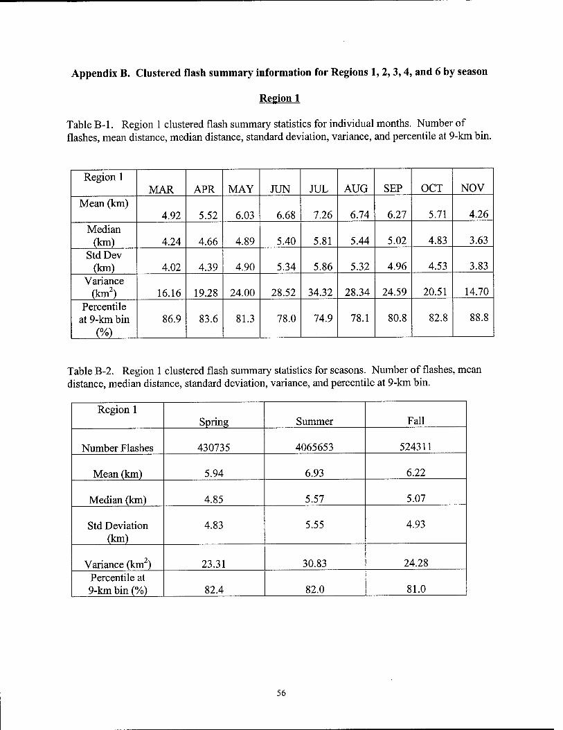
Appendix B. Clustered flash summary information for Regions 1,2,3,4, and 6 by season

Region 1

Table B-l. Region 1 clustered flash summary statistics for individual months. Number of flashes, mean distance, median distance, standard deviation, variance, and percentile at 9-km bin.

Region 1 MAR APR MAY JUN JUL AUG SEP OCT NOV

Mean (km) 4.92 5.52 6.03 6.68 7.26 6.74 6.27 5.71 4.26

Median (km) 4.24 4.66 4.89 5.40 5.81 5.44 5.02 4.83 3.63

Std Dev (km) 4.02 4.39 4.90 5.34 5.86 5.32 4.96 4.53 3.83

Variance (km2) 16.16 19.28 24.00 28.52 34.32 28.34 24.59 20.51 14.70

Percentile at 9-km bin

(%)

86.9 83.6 81.3 78.0 74.9 78.1 80.8 82.8 88.8

Table B-2. Region 1 clustered flash summary statistics for seasons. Number of flashes, mean distance, median distance, standard deviation, variance, and percentile at 9-km bin.

Region 1 Spring Summer Fall

Number Flashes 430735 4065653 524311

Mean (km) 5.94 6.93 6.22

Median (km) 4.85 5.57 5.07

Std Deviation (km)

4.83 5.55 4.93

Variance (km ) 23.31 30.83 24.28 Percentile at 9-km bin (%) 82.4 82.0 81.0

56

Frequency of clustered flashes to cluster center Region 1

500000 --

n- E

- - - d) s o .c to

■ Spring

DSummer

■ Fall

o Q>

E -

-

-

-

- - - - z

i- - - - - - - - -

o 1 ■pi LTJ,LI 1 L| 11-, FL n_ n n n n ■-■■-, r, „ 1 2 3 4 5 6 7 8 9 10 1 1 12 13 14 15 16 17 18 19 20 21 22 23 24 25 26 27 28 29 30

Distance form cluster center (km)

Figure B-l. Region 1 frequency distributions of flashes per km from cluster center. Frequencies for Spring, Summer, and Fall.

Cumulative histogram of distances from flash to cluster center Region 1

100

E

a a. m a O) ra c o

o> D. 0) > « 3 E 3 Ü

1 2 3 4 5 6 7 8 9 10 11 12 13 14 15 16 17 18 19 20 21 22 23 24 25 26 27 28 29 30

Distance from flash to cluster center (km)

Figure B-l. Region 1 cumulative frequency distribution of clustered flashes per km from cluster center. Distributions for Spring, Summer, and Fall.

57

Region 2

Table B-3. Region 2 clustered flash summary statistics for individual months. Number of flashes, mean distance, median distance, standard deviation, variance, and percentile at 9-km bin.

Region 2 MAR APR MAY JUN JUL AUG SEP OCT NOV

Mean (km) 4.75 4.86 5.80 6.43 6.30 6.11 5.98 6.60 5.09

Median (km) 3.84 3.94 4.60 5.12 4.97 4.80 4.76 5.30 4.19

Std Dev (km) 4.02 4.13 4.78 5.20 5.09 4.97 4.76 5.42 4.30

Variance (km2) 16.13 17.04 22.89 27.03 25.91 24.74 22.63 29.42 18.48

Percentile at 9-km bin (%) 87.8 87.0 82.3 79.7 80.5 81.5 82.4 78.8 85.7

Table B-4. Region 2 clustered flash summary statistics for seasons. Number of flashes, mean distance, median distance, standard deviation, variance, and percentile at 9-km bin.

Region 2 Spring Summer Fall

Number Flashes 656753 6717770 152908

Mean (km) 5.62 6.26 6.05

Median (km) 4.47 4.93 4.82

Std Deviation (km) 4.68 5.07 4.85

Variance (km2) 21.94 25.70 23.50 Percentile at 9-km bin (%) 83.6 80.7 82.0

58

Frequency of clustered flashes to cluster center Region 2

E

a. 600000

n 500000 -

i- 400000 - a

200000 -- — m- ■ =-

12 3 4 5

JUUUUry n^ FT-, n^ n n-, n-, i

10 11 12 13 14 15 16 17 18 19 20 21 22 23 24 25 26 27 28 29 30

Distance from cluster center (km)

Figure B-3. Region 2 frequency distributions of flashes per km from cluster center. Frequencies for Spring, Summer, and Fall.

Cumulative histogram of distances from flash to cluster center Region 2

£

0) a (A a> a ra c <v a 9) a a> >

E Ü

Figure B-4. Region 2 cumulative frequency distribution of clustered flashes per km from cluster center. Distributions Spring, Summer, and Fall.

59

Region 3

Table B-5. Region 3 clustered flash summary statistics for individual months. Number of flashes, mean distance, median distance, standard deviation, variance, and percentile at 9-km bin.

Region 3 MAR APR MAY JUN JUL AUG SEP OCT NOV

Mean (km) 7.43 7.90 8.83 9.09 8.96 8.62 8.32 8.04 7.44

Median (km) 6.38 6.64 7.22 7.24 7.17 6.86 6.70 6.63 6.28

Std Dev (km) 5.36 5.84 6.76 7.26 7.06 6.86 6.51 6.16 5.57

Variance (km2) 28.71 34.05 45.73 52.68 49.80 47.05 42.35 37.96 31.07

Percentile at 9-km bin

(%)

71.2 70.9 65.8 64.8 65.5 67.2 68.9 70.1 73.0

Table B-6. Region 3 clustered flash summary statistics for seasons. Number of flashes, mean distance, median distance, standard deviation, variance, and percentile at 9-km bin.

Region 3 Spring Summer Fall

Number Flashes 2988040 11424596 2159593

Mean (km) 8.55 8.90 8.22

Median (km) 7.03 7.10 6.66

Std Deviation (km) 6.51 7.07 6.40

Variance (km2) 42.42 50.00 40.93 Percentile at 9-km bin (%) 67.3 65.8 69.3

60

Frequency distribution of flashes to cluster center Region 3

1200000

12 3 4 5 6 7 10 11 12 13 14 15 16 17 18 19 20 21 22 23 24 25 26 27 28 29 30

Distance from cluster center (km )

Figure B-5. Region 3 frequency distributions of flashes per km from cluster center. Frequencies for Spring, Summer, and Fall.

Cumulative histogram of distances from flash to cluster center Region 3

1 2 3 4 5 6 7 8 9 10 1 1 12 13 14 15 16 17 18 19 20 21 22 23 24 25 26 27 28 29 30

Distance from flash to cluster center (km)

Figure B-6. Region 3 cumulative frequency distribution of clustered flashes per km from cluster center. Distributions for Spring, Summer, and Fall.

61

Region 4

Table B-7. Region 4 clustered flash summary statistics for individual months. Number of flashes, mean distance, median distance, standard deviation, variance, and percentile at 9-km bin.

Region 4 MAR APR MAY JUN JUL AUG SEP OCT NOV

Mean (km) 8.43 9.20 9.10 8.46 7.89 7.33 7.63 8.39 8.49

Median (km) 6.99 7.57 7.38 6.68 6.06 5.60 5.96 6.78 7.01

Std Dev (km) 6.24 6.84 6.99 6.82 6.59 6.15 6.23 6.53 6.36

Variance (km2) 39.00 46.74 48.90 46.46 43.44 37.82 38.83 42.58 40.49

Percentile at 9-km bin (%)

68.2 63.9 64.5 68.1 71.3 74.5 72.8 68.8 67.9

Table B-8. Region 4 clustered flash summary statistics for seasons. Number of flashes, mean distance, median distance, standard deviation, variance, and percentile at 9-km bin.

Region 4 Spring Summer Fall

Number Flashes 7803513 14063274 3615701

Mean (km) 9.01 7.91 7.97

Median (km) 7.36 6.11 6.35

Std Deviation (km) 6.82 6.55 6.35

Variance (km2) 46.56 42.93 40.28 Percentile at 9-km bin (%) 65.0 71.2 70.9

62

Frequency of clustered flashes to cluster center Region 4

1600000

£

1400000

1200000

S 1000000 -\- </> o

SZ V) ra 800000

J> 600000

E 3

400000

200000

■ Spring DSummer ■ Fall

Distance from cluster center (km)

Figure B-7. Region 4 frequency distributions of flashes per km from cluster center. Frequencies for Spring, Summer, and Fall.

Cumulative histogram of distances from flash to cluster center Region 4

1 2 3 4 5 6 7 8 9 10 11 12 13 14 15 16 17 18 19 20 21 22 23 24 25 26 27 28 29 30

Distance from flash to cluster center (km)

Figure B-8. Region cumulative frequency distribution of clustered flashes per km from cluster center. Distribution for Spring, Summer, and Fall.

63

Region 6

Table B-9. Region 6 clustered flash summary statistics for individual months. Number of flashes, mean distance, median distance, standard deviation, variance, and percentile at 9-km bin.

Region 6 MAR APR MAY JUN JUL AUG SEP OCT NOV

Mean (km) 7.71 8.07 8.91 8.35 8.57 7.90 7.62 8.21 7.04

Median (km) 6.56 6.71 7.10 6.44 6.57 6.03 5.90 6.78 6.13

Std Dev (km) 5.62 6.04 7.05 6.97 7.16 6.66 6.39 6.26 5.15

Variance (km2) 31.60 36.52 49.66 48.65 51.23 44.42 40.88 39.13 26.51

Percentile at 9-km bin

(%)

72.2 70.3 66.0 69.3 68.1 71.7 73.4 68.7 75.6

Table B-10. Region 6 clustered flash summary statistics for seasons. Number of flashes, mean distance, median distance, standard deviation, variance, and percentile at 9-km bin.

Region 6 Spring Summer Fall

Number Flashes 3278341 10764828 992038

Mean (km) 8.65 8.33 7.66

Median (km) 6.97 6.39 6.01

Std Deviation (km) 6.76 6.98 6.33

Variance (km ) 45.76 48.74 40.03 Percentile at 9-km bin (%) 67.4 69.4 73.0

64

Frequency of clustered flashes to cluster center Reg ion 6

1200000

01 a 800000 --[■

<A

£ CO n

o

600000 --

k. 01 n E 3 Z

400000 --

200000 -|

J\. J 41 ^ 41 ^ PH pn 1 2 3 4 5 6 7 8 9 10 1 1 12 13 14 15 16 17 18 19 20 21 22 23 24 25 26 27 28 29 30

Distance from cluster center (km)

Figure B-9. Region 6 frequency distributions of flashes per km from cluster center. Frequencies for Spring, Summer, and Fall.

Cumulative histogram of distances from flash to cluster center Region 6

1 2 3 4 5 6 7 8 9 10 11 12 13 14 15 16 17 18 19 20 21 22 23 24 25 26 27 28 29 30

Distance from flash to cluster center (km)

Figure B-10. Region 6 cumulative frequency distribution of clustered flashes per km from cluster center. Distribution for Spring, Summer and Fall.

65

Appendix C. Isolated flash summary information for Regions 1, 2, 3,4, and 6 by seasons

Region 1

Table C-l. Region 1 isolated flash summary statistics for individual months. Mean distance, median distance, standard deviation, variance, and the distance at the 90l percentile.

Region 1 MAR APR MAY JUN JUL AUG SEP OCT NOV

Total # isolated flashes 1145 5298 25549 53607 56142 44446 21751 5874 2749 Mean (km) 47.82 14.72 53.83 41.08 76.77 56.62 111.84 62.04 73.07

Median (km) 21.44 10.34 20.12 24.01 22.99 19.43 48.00 17.39 30.69

Std Dev (km) 71.14 20.86 127.17 68.58 146.21 100.22 137.48 98.36 105.32

Variance (km2) 5060 435 16173 4703 21377 10044 18901 9675 11091 90th

Percentile (km)

58 61 58 53 51 52 54 54 55

66

Freequency of isolated flashes to nearest flash Region 1 April/July /October

3000

T- T- OJ OJ <\J

Distance from nearest flash (km)

Figure C-l. Region 1 frequency distributions of isolated flashes per km to the nearest flash. Frequencies for April, July, and October.

Cumulative frequency of distances from isolated flashes to nearest flash Region 1 April July October

100

90 , . E an j£ L.

a. 70 *■■■*

u n 60

«-» c 0) o 50 k. 0) a. 40 0) > *->

30 3

o 20

10

n^^^^^

♦ April

-«-July

October If

- i i i i i 11 i 11 i i i i 11 i i i i i i i i i i i i i i i i i i i i i i i i 11 i ) i i i' i i i i i i i 11 ' i i i'

f-Tj-h-ocoeDOiCNjmco-r-Tth-ococDOCNjiooor-^j-^-o T-T-T-T-c\icvjCMCocooO'^-'>t'*'<tmmmcDCDCc>r~-

Distance from nearest flash (km)

Figure C-2. Region 1 cumulative frequency distribution s of isolated flashes per km from nearest flash. Distributions for April, July, and October.

67

Region 2

Table C-2. Region 2 isolated flash summary statistics for individual months. Mean distance, median distance, standard deviation, variance, and the distance at the 90l percentile.

Region 2 MAR APR MAY JUN JUL AUG SEP OCT NOV

Total # isolated flashes 4775 7266 28190 43418 74708 66344 40781 11831 8534 Mean (km) 97.66 77.06 106.34 53.22 29.77 23.72 52.76 77.56 92.36

Median (km) 64.44 14.99 20.09 21.51 18.51 17.83 23.91 19.35 58.26

Std Dev (km) 104.67 263.01 306.23 64.59 58.65 29.52 88.42 98.55 502.33

Variance (km2) 10956 69175 93774 1017 3439 871 7818 6072 7225 90th

Percentile (km)

66 65 58 50 51 53 54 54 56

68

Frequency of isolated flashes to nearest flash Region 2 April/July/October

4000

Distance from nearest flash (km)

Figure C-3. Region 2 frequency distributions of isolated flashes per km to the nearest flash. Frequencies for April, July, and October.

Cumulative frequency of distances from isolated flashes to nearest flash Region 2 April July October

100

E

a. o at re +■* c 0) u a> o. a> >

^3 re 3 E 3 o

(D CNJ m co T— M- r-- o co CD o> CM in oo T— ■* 1^- O <N <N CSJ co CO co ■* ■* ■<* ■tf m io io CD CD CD 1^-

Distance from nearest flash (km)

Figure C-4. Region 2 cumulative frequency distributions of isolated flashes per km from the nearest flash. Distributions for April, July, and October.

69

Region 3

Table C-3. Region 3 isolated flash summary statistics for individual months. Mean distance, median distance, standard deviation, variance, and the distance at the 90l percentile.

Region 3 MAR APR MAY JUN JUL AUG SEP OCT NOV

Total # isolated flashes 13140 26314 67585 85168 80919 66901 39628 25688 1168

0 Mean (km) 24.40 20.87 28.92 41.85 28.16 48.29 27.56 26.66 33.24

Median (km) 19.31 18.65 17.90 20.87 18.44 24.93 23.89 17.91 20.67

Std Dev (km) 24.30 17.63 65.48 79.57 40.83 119.69 19.02 32.64 58.66

Variance (km2) 590 310 4287 6331 1667 14324 361 1065 3441 90th

Percentile (km)

39 39 41 42 42 45 46 43 43

70

Frequency of isolated flashes to nearest flash Region 3 April/July/October

■ April □ July

■ October

tKto iiMWiiMWV (DO>c\iwco->--<i-i-.oc2tDg><N[noor-;tfr-- T-T-CMCNCMCOCOCOTJ-^a-TfTfWWWtOCDCD

Distance from nearest flash (km)

Figure C-5. Region 3 frequency distributions of isolated flashes per km to the nearest flash. Frequencies for April, July, and October.

Cumulative frequency of distances from isolated flashes to nearest flash Region 3 April July October

100

E

<D a. ID O) n •** c 0) u u 0) a 0) .> "^ m 3 E 3 o

co (D en CM T- T- T- CM

Distance from nearest flash (km)

Figure C-6. Region 3 cumulative frequency distributions of isolated flashes per km from the nearest flash. Distributions for April, July, and October.

71

Region 4

Table C-4. Region 4 isolated flash summary statistics for individual months. Mean distance ,th median distance, standard deviation, variance, and the distance at the 90 percentile.

Region 4 MAR APR MAY JUN JUL AUG SEP OCT NOV

Total # isolated flashes 47027 59597 73167 76841 79244 67455 42448 35403 23862 Mean (km) 24.39 24.26 26.25 30.69 47.72 30.49 25.36 22.69 32.68

Median (km) 18.92 17.35 17.35 17.38 18.72 18.62 19.52 17.12 20.36

Std Dev (km) 30.43 40.11 48.08 71.85 102.67 56.94 46.23 33.00 58.86

Variance (km2) 926 1609 2311 5162 10541 3242 2623 1088 3464 90th

Percentile (km)

39 37 40 47 47 51 50 44 46

72

Frequency of isolated flashes to nearest flash Region 4 April/July/October

4500

_g 1500 E Z 1000

Distance from nearest flash (km)

Figure C-7. Region 4 frequency distributions of isolated flashes per km to the nearest flash. Frequencies for April, July, and October.

Cumulative frequency of distances from isolated flashes to nearest flash Region 4 April July October

Distance from nearest flash (km)

Figure C-8. Region 4 cumulative frequency distributions of isolated flashes per km from the nearest flash. Distributions for April, July, and October.

73

Region 6

Table C-5. Region 6 isolated flash summary statistics for individual months. Mean distance, median distance, standard deviation, variance, and the distance at the 90th percentile.

Region 6 MAR APR MAY JUN JUL AUG SEP OCT NOV

Total # isolated flashes 11839 33769 42115 51170 46763 23645 16567 8238 5996 Mean (km) 31.64 17.83 34.04 41.69 30.90 22.70 32.20 24.95 27.25

Median (km) 14.36 17.23 19.86 18.96 19.16 12.87 18.85 18.45 19.55

Std Dev (km) 71.25 15.29 58.41 95.59 49.12 21.76 52.95 26.92 32.40

Variance (km2) 5076 233 3412 9137 2412 473 2803 724 1049 90th

Percentile (km)

39 48 41 45 47 40 50 48 48

74

Frequency of isolated flashes to nearest flash Region 6 April/July/October

2500

Si-- o CD N.

Distance from nearest flash (km)

Figure C-9. Region 6 frequency distributions of isolated flashes per km to the nearest flash. Frequencies for April, July, and October.

Cumulative frequency of distances from isolated flashes to nearest flash Region 6 April July October

100

E im 0) a

O) (0 <** c o

0) a v > n 3 E 3 o

S fc p

Distance from nearest flash (km)

Figure C-10. Region 6 cumulative frequency distributions of isolated flashes per km from the nearest flash. Distributions for April, July, and October.

75

Appendix D. List of Acronyms

AFIT

AFOSH

CDT

CG

dBZ

DBSF

IDL

IMPACT

MDF

NLDN

NSSL

SCIT

TOA

UTC

WATADS

WSR-88D

Air Force Institute of Technology

Air Force Operational Safety Handbook

Central Daylight Time

Cloud-to-ground

Decibel

Distance Between Successive Flash

Interactive Data Language

IMProved Accuracy from Combined Technology

Magnetic Detection Finders

National Lightning Detection Network

National Severe Storms Laboratory

Storm Cell Identification and Tracking

Time-of-Arrival

Universal Time Code

WSR-88D Algorithm Testing and Display System

Weather Surveillance Radar - 88 Delta

76

Vita

Captain Tamara L. Parsons was born on 14 March 1970 in Johnson City, New York. She

graduated from Montrose Area High School, Montrose, Pennsylvania in 1988 and entered the

undergraduate meteorology program at The Pennsylvania State University in State College,

Pennsylvania. While attending Perm State, she enrolled in the Air Force Reserve Officer

Training Corps. She graduated with a Bachelor of Science degree in Meteorology and was

concurrently commissioned as a 2nd Lieutenant in the United States Air Force in May 1992.

While waiting to come on active duty she worked for Perm State as a research assistant on the

TOGA CORE project and spent several months on the island of Kavieng in Papua New Guinea.

Captain Parsons' first assignment was to an Army Installation in Illesheim, Germany,

where she became the Officer in Charge of the Cadre Weather Team. While in Germany she

went on numerous deployments with the Army and participated in several NATO exercises.

Captain Parsons' next assignment took her to Vandenberg AFB, California, where she

worked as a Launch Weather Officer for military, DoD, and commercial space programs. She

also served as the Flight Commander, Operations Support in the 30th Weather Squadron while at

Vandenberg AFB.

In August 1998, she entered the graduate meteorology program in the School of

Engineering at the Air Force Institute of Technology. Following graduation, Captain Parsons

will be assigned to HQ PACAF/DOWO, Hickam AFB, in Hawaii.

Permanent Address: 901 Pimlico Drive Apt 2D Centerville OH 45459

77

REPORT DOCUMENTATION PAGE Form Approved OMB No. 0704-0188

Pubüc reporting burden tor this collection of information is estimated to average 1 hour per response, including the time for reviewing Instructions, searching existing data sources, gathering and maintaining the data needed, ana completing and reviewing the cofiection of information. Send comments regarding this burden estimate or any other aspect of this collection of information, including suggestions for reducing this burden, to Washington Headquarters Services, Directorate for information Operations and Reports, 1256 Jefferson Davis Highway- Suite 1204, Arlington, VA 22202-4302, and to the Office of Management and Budget, Paperwork Reduction Project {0704-0188}, Washington, DC 20503.

1. AGENCY USE ÖNLV /Leave blank) 2. REPORT BATE

March 2000 5. REPflBT TVPE AND DATES COVERED

Master's Thesis 4. TITLE ANb SUBTITLE DETERMINING THE HORIZONTAL DISTANCE DISTRIBUTION OF CLOUD-TO-GROUND LIGHTNING

S. FUN6IN0 NUMBEAS

6. AUTHOR(S)

Tamara L. Parsons, Captain, USAF

7. PERFORMING ORGANIZATION NAME(S) AND ADDRESS(ES) Air Force Institute of Technology Graduate School of Engineering and Management (AFIT/EN) 2950 P Street, Building 640 WPAFB OH 45433-7765

8. PERFORMING ORGANIZATION REPORT NUMBER

AFIT/GM/ENP/OOM-09

9. SPONSORING/MONITORING AGENCY NAME(S) AND ADDRESS(ES) Lt Col William H. Bauman III AFRL/XPPR WPAFB OH 45433-7765 DSN: 785-4760

16. SP6NS6RIN6/M6NIT6RING AGENCY REPORT NUMBER

H. SUPPLEMENTARY NOTES Advisor: Maj Gary Huffmes, ENP, DSN: 785-3636 ext. 4511

12«. DISTRIBUTION AVAILABILITY STATEMENT

APPROVED FOR PUBILC RELEASE: DISTRIBUTION UNLIMITED

12b. DISTRIBUTION eöDt

13. ABSTRACT (Maximum 200 words) This research effort attempted to quantify what constitutes a safe distance when lightning is present.

The method used in this research project groups lightning flashes into clusters using spatial and temporal constraints. However, not all flashes meet the time and distance criteria for clustering and remained outside of the grouped flashes and as such are identified as isolated flashes. These isolated flashes are outliers in the data set, but are precisely the flashes that prove most dangerous. For Ulis reason not only were the distances between each flash and cluster center studied, but also the distances between each isolated flash and its nearest neighboring flash. Distributions for both distances were stud^d for the continental U.S. by season.

A common safety radius is 5 nautical miles, just less than 9.5 km. For all regions, anywhere from 16% to : 5.: clustered flashes occurred beyond 9.5 km from the cluster center and 71 % to 81 % of die isolated flashes occurr;C a, distances beyond 9.5 km from the nearest flash. Cumulative frequency distributions of historical lightning data can l>. used to find the probability of having lightning at a particular distance. In this way an acceptable level of risk can b< der.-iriined and then a "safe" distance found.

U.SUBJECTTIBMS Lightning, Cloud-to-Ground Lightning, Distance lightning travels, Lightning safety, Distance Between Successive Flashes

16. NUMBER OF PAGES

77

\1. SECURITV CLASSIFIOATION I iä. sfeURiTY CLASSIFICATION 11s. SECURITY CLASSIFICATION OF REPORT OF THIS PAGE OF ABSTRACT

16. PRICE CODE

20. LIMITATION oP AöSTRACT

UL UNCLASSIFIED UNCLASSIFIED UNCLASSIFIED Standard Form 298 (Rev. 2-89) (KG Prescribed by ANSI S:d. 239.13 Designed using Perforr VVHS.DiOP., Get 34