determining the shape of a human vocal tract from pressure...

1

Inverse Problems

Determining the shape of a human vocal tract from pressure measurements at the lips

Tuncay Aktosun1,4, Alicia Machuca2 and Paul Sacks3

1 Department of Mathematics, University of Texas at Arlington, Arlington, TX 76019-0408, United States of America2 Department of Mathematics and Computer Science, Texas Woman’s University, Denton, TX 76204, United States of America3 Department of Mathematics, Iowa State University, Ames, IA 24061, United States of America

E-mail: [email protected]

Received 4 May 2017, revised 14 August 2017Accepted for publication 24 August 2017Published 3 October 2017

AbstractThe inverse problem of determining the cross-sectional area of a human vocal tract during the utterance of a vowel is considered in terms of the data consisting of the absolute value of sound pressure at the lips. If the upper lip is curved downward during the utterance, it is shown that there may be up to an M-fold nonuniqueness in the determination, where M is the maximal number of eligible resonances associated with a related Schrödinger operator. Each of the M such distinct candidates for the vocal-tract area corresponding to the same absolute pressure is uniquely determined. The mathematical theory is presented for the recovery of each candidate for the vocal-tract area, and the admissibility criterion for each of the M candidates to be a vocal-tract radius is specified. On the other hand, if the upper lip is horizontal or curved upward during the utterance, then the inverse problem has a unique solution. The theory developed is illustrated with some examples.

Keywords: inverse scattering, speech acoustics, shape of vocal tract

(Some figures may appear in colour only in the online journal)

1. Introduction

The production of human speech is similar [7, 8, 13, 15–17] in principle to the sound produc-tion in tubular musical instruments. The inhaled air travels from the mouth down the vocal tract, a tube about 14–20 cm in length with a pair of lips at the mouth and another pair of lips

T Aktosun et al

Determining the shape of a vocal tract

Printed in the UK

115002

INPEEY

© 2017 IOP Publishing Ltd

33

Inverse Problems

IP

1361-6420

10.1088/1361-6420/aa882d

Paper

11

1

33

Inverse Problems

IOP

2017

4 Author to whom any correspondence should be addressed.

1361-6420/17/115002+33$33.00 © 2017 IOP Publishing Ltd Printed in the UK

Inverse Problems 33 (2017) 115002 (33pp) https://doi.org/10.1088/1361-6420/aa882d

mailto:[email protected]

http://crossmark.crossref.org/dialog/?doi=10.1088/1361-6420/aa882d&domain=pdf&date_stamp=2017-10-03

publisher-id

doi

https://doi.org/10.1088/1361-6420/aa882d

2

known as the vocal cords at the opposite end. The inhaled air passes between the vocal cords and travels to the lungs through another tube known as the voice box or the larynx. From the lungs the air travels back and enters the vocal tract through the glottis (the opening between the vocal cords). The pressure created at the glottis puts the nearby air molecules in the vocal tract into longitudinal vibrations. These vibrations are responsible for the propagation of the sound pressure in the vocal tract. The pressure wave comes out of the mouth and is transmitted in the air to a person’s ears or to a microphone.

Human speech consists of basic units known as phonemes. For example, when we utter the word ‘book’ we in succession produce the three phonemes /b/, /u/, and /k/, each lasting about 0.1 s. The phonemes can be classified into two main groups as vowels and consonants. For the mathematical description of vowel production, one can satisfactorily ignore the articulators (such as the tongue) and assume that the cross-sectional area A(x) of the vocal tract as a func-tion of the distance from the glottis is the only factor responsible for the produced sound. We mention that x = 0 corresponds to the glottis and the lips are located at x = �, where � denotes the length of the vocal tract.

During the production of each vowel, the shape of the vocal tract can be assumed not to depend on time. In some sense this is analogous to watching a movie, where each frame con-tains a static image and lasts for a short period. The continuous movie is perceived and the continuous speech is heard, respectively, as we watch a succession of static images and as we encounter a succession of static shapes of the vocal tract. The length � of the vocal tract depends on the individual speaker, and it can be satisfactorily assumed that � does not change during the production of a particular phoneme. Mathematically, one can ignore the bending of the vocal tract and assume that the cross-sectional area at each x-value is circular with radius r(x), where

A(x) = π[r(x)]2. (1.1)

Let us use p(x, t) and v(x, t) for the pressure and the volume velocity, respectively, in the vocal tract at location x and at time t. Let ν denote the frequency measured in Hz (Hertz), ω the angular frequency in rad s−1, k the angular wavenumber in rad cm−1, and λ the wavelength in cm. In other words, k in radians per centimeter shows the number of waves per centimeter divided by 2π. These quantities are related to each other as

ω = kc, ω = 2πν, νλ = c, (1.2)

where c is the sound speed in the vocal tract. The value of c can be assumed to be a constant, which is about 34 300 cm s−1 at room temperature. From (1.2) we see that

k =2πν

c,

and hence k can be viewed as a constant multiple of the frequency. The audible frequencies usually range from 20–20 000 Hz for human beings. So, 20 Hz corresponds to k = 0.0037 rad cm−1 and 20 000 Hz corresponds to k = 3.7 rad cm−1. There is one more relevant constant, namely the air density μ used in the description of the sound propagation in the vocal tract, and its value is about 0.0012 grams per cubic centimeter.

If the propagating pressure wave p(x, t) is monochromatic, it contains only one sinusoidal component at a single frequency. A similar remark also applies to the volume velocity v(x, t). In general, each of p(x, t) and v(x, t) is a linear combination of sinusoidal components at many frequencies, and they can be expressed as

p(x, t) =1

2π

∫ ∞

−∞dk P(k, x) eiωt, v(x, t) =

12π

∫ ∞

−∞dk V(k, x) eiωt, (1.3)

T Aktosun et alInverse Problems 33 (2017) 115002

3

where we refer to P(k, x) and V(k, x) as the pressure and the volume velocity, respectively, in the frequency domain. The use of the complex exponent eiωt in (1.3) is mathematically convenient. One can certainly avoid using negative frequencies in (1.3) by noting [1, 2] that

P(−k, x) = P(k, x)∗, V(−k, x) = V(k, x)∗, k ∈ R, (1.4)

where R := (−∞,+∞) and the asterisk denotes complex conjugation.The time factor eiωt in (1.3) is the acoustician’s convention, whereas it is customary to use

the time factor e−iωt as the physicist’s convention. In this paper we use the former convention, and hence we visualize eikx in the frequency domain as the wave component eikx+iωt in the time-domain signal, which is a plane wave moving in the negative x-direction. Similarly, e−ikx can be visualized as a plane wave moving in the positive x-direction.

Throughout our paper we assume that the vocal-tract radius belongs to class A specified below.

Definition 1.1. The vocal-tract radius r(x) is said to belong to class A if the following conditions are satisfied:

(a) The function r(x) is real valued and positive on x ∈ (0, �). (b) The function r(x) has positive limits as x → 0+ and as x → �−. (c) The derivative function r′(x) is continuous for x ∈ (0, �) and has finite limits as x → 0+

and as x → �−. (d) The second-derivative function r′′(x) is integrable on x ∈ (0, �).

Without any loss of generality, we let

r(0) := r(0+), r′(0) := r′(0+), r(�) := r(�−), r′(�) := r′(�−).

Our primary goal in this paper is the analysis of the inverse problem of recovery of the vocal-tract shape when we know the absolute sound pressure at the lips at all positive frequen-cies during the production of a vowel. Mathematically, this is equivalent to the recovery of A(x) for x ∈ (0, �) when our input data set consists of |P(k, �)| for k > 0. In the analysis of our inverse problem we assume that the value of � is known. At the end of section 4 we com-ment on the solution of the inverse problem if the value of � is not known. With the help of (3.33), (3.34) and (3.36), we can argue that the input data set in the audible frequency range is sufficient for a satisfactory approximate recovery. Because of (1.1), we can equivalently recover r(x) instead of A(x). Furthermore, with the help of (1.4) we see that our input data set is equivalent to the data set |P(k, �)| for k ∈ R. Since we use the CGS system of units, the distance x and the radius are measured in centimeters, the area A(x) in square centimeters, and the pressure |P(k, �)| in dynes per square centimeter.

The associated direct problem can be described as the determination of the absolute pres-sure at the lips when the vocal-tract area function is known. A solution to this direct problem is explicitly given [1, 2] with the help of the Jost function and the Jost solution associated with a corresponding self-adjoint Schrödinger operator on the half line. A solution to the inverse problem has been given in [1, 2] under a certain additional restriction on r(x) that is equivalent to the absence of bound states in the associated Schrödinger operator. In our current paper, we study our inverse problem without that restriction. We show that the corresponding Schrödinger operator does not have any bound states for certain vowels but it has exactly one bound state for the remaining vowels. We provide a characterization of the absence or pres-ence of a bound state in terms of the bending of the vocal-tract radius at the upper lip, i.e. in terms of the sign of r′(�). From the appearance of the lips during a vowel utterance, one may tell what the sign of r′(�) is. For example, for the vowels /u/, /a/, and /o/, we have r′(�) = 0,


4

r′(�) > 0, and r′(�) < 0, respectively. We show that there are no bound states if r′(�) � 0 and that there is exactly one bound state if r′(�) < 0. We provide the solution to our inverse problem in the possible presence of a bound state, and we also characterize the uniqueness or nonuniqueness that may be occurring in the presence of a bound state.

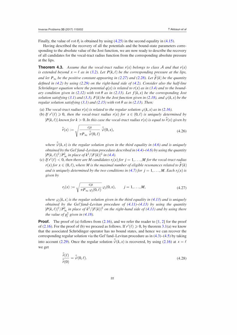
Our paper is organized as follows. In section 2 we present the preliminaries needed for later sections, by providing the solution to the direct problem in two different ways. In theo-rem 2.1 we provide the explicit expressions for the pressure and volume velocity in the vocal tract in terms of the unique solution f (k, x) to the initial-value problem consisting of (2.10) and (2.14) as well as the quantity F(k) appearing in (2.18). In theorem 2.2 we indicate that the solution to the direct problem could alternatively be obtained by solving the initial-value problem related to (2.2), (2.24) and (2.26). The result in theorem 2.1 is needed for the form-ulation of our inverse problem. The results presented in the finite interval x ∈ (0, �) in sec-tion 2 are extended to the half line in section 3, and this allows us to exploit the properties of the absolute pressure at the lips in terms of the absolute value of the Jost function, based on the important relationship stated in (2.29). In section 3, we elaborate on that relationship and show that if r′(�) � 0 then the associated Jost function does not have any bound-state zeros and also show that if r′(�) < 0 then the Jost function has exactly one bound-state zero. In section 4 we provide the solution to our inverse problem, with the help of the Gel’fand–Levitan method and alternatively with the help of the Marchenko method. We show that the vocal-tract radius r(x) can uniquely be determined from the absolute pressure if r′(�) � 0. On the other hand, if r′(�) < 0, we show that, corresponding to the same absolute pressure, there are M candidates for r(x) with r′(�) < 0 in addition to the candidate for r(x) with r′(�) � 0. We show that M is the maximal number of eligible resonances [4] for an associated Schrödinger equation and is uniquely determined by the absolute pressure. In section 4 we also prove that each one of the (M + 1) candidates for r(x) corresponding to the same absolute pressure is uniquely determined. From definition 1.1(b), we know that only those candidates for which the constructed r(x) satisfying r(�) > 0 are admissible as the vocal-tract radii, and we present an equivalent admissibility criterion. In section 5, under the assumption that r′(�) � 0, we present a time-domain method to solve our inverse problem, providing an alternate method to the two frequency-domain methods presented in section 4. Finally, in section 6 we illustrate our results with some examples. In particular, we use the vocal-tract area data from [18] and compute the corresponding absolute pressure at the lips by using the alternate method based on theorem 2.2. We then use that constructed pressure data set as input to the time-domain method described in section 5 and determine the corresponding vocal-tract cross-sectional area. The input area from [18] and the computed area are shown in the first plot in figure 1, indicating a fairly accurate numerical solution to our inverse problem.

2. The solution to the direct problem

In this section we review the acoustics in the vocal tract, and we associate it with the Schrödinger equation given in (2.10) for x ∈ (0, �), where the potential q(x) is related to the vocal-tract radius function r(x) as in (2.11). In (2.21) and (2.22), respectively, we provide explicit expressions for the pressure P(k, x) and the volume velocity V(k, x) in terms of r(x) and the key quantity F(k) given in (2.18). By expressing the absolute pressure at the lips explicitly as in (2.23), we provide a solution to the direct problem of recovery of the absolute pressure at the lips from the vocal-tract radius function. Via theorem 2.2 we show that the solution of the direct problem can alternatively be achieved by solving the system (2.2) with the initial conditions as in (2.24) and (2.26). Even though the latter method is more straightfor-ward than the former method, the former is needed in the formulation of the inverse problem.


5

It is reasonable [15, 16] to assume that the sound propagation in the vocal tract is lossless and planar and that the acoustics in the vocal tract are governed [7, 8, 15–17] by

{A(x) px(x, t) + µ vt(x, t) = 0,

A(x) pt(x, t) + c2µ vx(x, t) = 0,

(2.1)

where t > 0 and x ∈ (0, �), and the subscripts denote the appropriate partial derivatives. Using (1.1) and (1.3) in (2.1) we obtain

{πr(x)2 P′(k, x) + icµk V(k, x) = 0,

cµV ′(k, x) + iπk r(x)2 P(k, x) = 0, (2.2)

where the prime denotes the x derivative. Eliminating V(k, x) in (2.2), we get the Webster horn equation

[r(x)2 P′(k, x)]′ + k2 r(x)2 P(k, x) = 0, x ∈ (0, �), (2.3)

or eliminating P(k, x) in (2.2) we get[

V ′(k, x)r(x)2

]′+ k2 V(k, x)

r(x)2 = 0, x ∈ (0, �). (2.4)

In order to solve (2.2) uniquely, we need two side conditions, which we can choose by specifying the glottal volume velocity v(0, t) and by assuming that the pressure wave at the lips goes only out of the mouth, not into the mouth. One particular choice for v(0, t) is given by

v(0, t) = δ(t), (2.5)

where δ(t) is the Dirac delta distribution. Comparing with the second equality in (1.3) we see that (2.5) is equivalent to

V(k, 0) = 1, (2.6)

which corresponds to a unit-amplitude, sinusoidal volume velocity at the glottis at any angular wavenumber k. With the help of the first line of (2.2), we see that (2.6) is equivalent to

P′(k, 0) = − icµkπ r(0)2 . (2.7)

0 2 4 6 8 10 12 14 16 18

distance from glottis (cm)

0

0.5

1

1.5

2

2.5

3

3.5

4

4.5ar

ea (

cm2)

cross sectional area for vowel /ae/

computed cross sectional areaarea data from [18]

0 0.5 1 1.5 2 2.5 3

k (rad/cm)

0

50

100

150

200

250

pres

sure

(dy

n/cm

2)

pressure at the lips

Figure 1. A(x) for /æ/ and |P(k, �)| at the lips, respectively, in examples 6.2 and 6.3.


6

The second side condition is equivalent to rejecting the wave component proportional to eik�+ikct and accepting only the wave component proportional to e−ik�+ikct in the expression for p(x, t) when x = �. It is known [1, 2] that such a condition is equivalent to

P′(k, �) = −[

ik +r′(�)r(�)

]P(k, �). (2.8)

With the help of (2.2), we see that (2.8) is equivalent to

k2V(k, �) =[

ik +r′(�)r(�)

]V ′(k, �). (2.9)

By letting

ψ(k, x) := r(x)P(k, x),

we can transform (2.3) into the Schrödinger equation

ψ′′(k, x) + k2ψ(k, x) = q(x)ψ(k, x), x ∈ (0, �), (2.10)

where the potential q(x) is related to the vocal-tract radius r(x) via

q(x) :=r′′(x)r(x)

, x ∈ (0, �). (2.11)

When r(x) belongs to class A specified in definition 1.1, the potential q(x) is real valued and integrable on x ∈ (0, �). In order to analyze the direct and inverse problems associated with (2.10), it is convenient to supplement (2.10) with the boundary condition [5, 9, 11, 12]

ψ′(k, 0) + (cot θ)ψ(k, 0) = 0, (2.12)

where the real-valued boundary parameter cot θ is related to the vocal-tract radius as

cot θ = − r′(0)r(0)

. (2.13)

We remark that the real parameter θ in (2.12) is allowed to take any value in the interval (0,π) and hence cot θ can be any number in the interval (−∞,+∞).

Two particular solutions to (2.10) are relevant for (2.3). One of these is the solution f (k, x) satisfying the initial conditions

f (k, �) = eik�, f ′(k, �) = ik eik�. (2.14)

Since k appears as k2 in (2.10), the quantity f (−k, x) is also a solution to (2.10), and it follows from (2.14) that, for each fixed real nonzero k, the functions f (k, x) and f (−k, x) are linearly independent. In section 3 we will relate f (k, x) to the Jost solution to the half-line Schrödinger equation (3.1) with the asymptotics eikx[1 + o(1)] as x → +∞.

The second relevant particular solution to (2.10) is the solution ϕ(k, x) satisfying the initial conditions

ϕ(k, 0) = 1, ϕ′(k, 0) = − cot θ, (2.15)

where cot θ is the boundary parameter appearing in (2.12). The solution ϕ(k, x) is related to the vocal-tract radius r(x) as [1, 2]

ϕ(0, x) =r(x)r(0)

, x ∈ (0, �), (2.16)


7

which plays a key role in solving our inverse problem. One can derive (2.16) by relating (2.10) at k = 0 and (2.15) to (2.11) and (2.13). In section 3 it will become clear that ϕ(k, x) satisfying (2.10) and (2.15) is the restriction to x ∈ (0, �) of the regular solution [5, 11–13] to the half-line Schrödinger equation (3.1) with the initial conditions (2.15).

With the help of the solution f (k, x) and the boundary parameter cot θ appearing in (2.12), let us define

F(k) := −i [ f ′(k, 0) + (cot θ) f (k, 0)] , (2.17)

and hence for the specific boundary parameter in (2.13) we obtain

F(k) = −i[

f ′(k, 0)− r′(0)r(0)

f (k, 0)]

, (2.18)

which will be useful in our analysis of the direct and inverse problems for the vocal tract. It is known that [1, 2]

F(k) = k + O(1), k → +∞, (2.19)

F(−k) = −F(k)∗, k ∈ R. (2.20)

The pressure and the volume velocity satisfying the two side conditions mentioned earlier can be evaluated uniquely and explicitly, as indicated in the following theorem. A proof is omitted and the reader is referred to [1] for a proof.

Theorem 2.1. Assume that the vocal-tract radius r(x) belongs to class A specified in definition 1.1. Then:

(a) The Webster horn equation (2.3) with the boundary conditions given in (2.7) and (2.8) has a unique solution, which is given by

P(k, x) = − cµk f (−k, x)π r(0) r(x)F(−k)

, x ∈ (0, �), (2.21)

where f (k, x) is the solution to (2.10) satisfying (2.14) and F(k) is the quantity given in (2.18). Similarly, (2.4) with the boundary conditions given in (2.6) and (2.9) is uniquely solvable, and the solution is given by

V(k, x) = − i r(x)r(0)F(−k)

[f ′(−k, x)− r′(x)

r(x)f (−k, x)

], x ∈ (0, �). (2.22)

(b) The quantities P(k, x) and V(k, x) are well defined for each k � 0 and x ∈ (0, �).

Using (2.14) and (2.20) in (2.21), the absolute pressure at the lips is seen to be

|P(k, �)| = cµkπ r(0) r(l) |F(k)|

, k ∈ (0,+∞). (2.23)

Having obtained (2.23), we can summarize the steps for a solution to our direct problem as follows:

(a) Given r(x), evaluate q(x) defined in (2.11). (b) Use q(x) in (2.10), solve the initial-value problem consisting of the linear homogeneous

differential equation (2.10) with the initial conditions (2.14), and hence recover f (k, x) for x ∈ (0, �).

(c) Using (2.18), evaluate the key quantity F(k).


8

(d) Determine the absolute pressure |P(k, �)| via (2.23).

The procedure described in (a)–(d) above is not necessarily a straightforward way of solving the direct problem. Its importance, however, comes from the fact that it relates the vocal-tract radius r(x) to the key quantity F(k) appearing in (2.23), and this is crucial in the formulation of our inverse problem.

With the goal of providing an alternate solution to our direct problem, let us define

P(k, x) :=P(k, x)P(k, �)

, V(k, x) :=V(k, x)P(k, �)

, (2.24)

where P(k, x) and V(k, x) are the pressure and volume velocity given in (2.21) and (2.22), respectively. From (2.6) and the second identity in (2.24) we see that

P(k, �) =1

V(k, 0). (2.25)

Theorem 2.2. Assume that the vocal-tract radius r(x) belongs to class A specified in defi-nition 1.1. Then, for each k > 0, the pair of quantities P(k, x) and V(k, x) defined in (2.24) forms the unique solution to the initial-value problem consisting of the first-order system (2.2) and the initial conditions at x = � given by

P(k, �) = 1, V(k, �) =1

cµ

[A(�) +

A′(�)

2ik

], (2.26)

where A(x) is the area function related to the vocal-tract radius as in (1.1).

Proof. From theorem 2.1(b) we know that P(k, x) and V(k, x) are well defined, and hence from (2.24) we conclude that P(k, x) and V(k, x) are well defined, provided P(k, �) �= 0. We confirm later in theorem 3.2(b) that P(k, �) �= 0 for k > 0. Since the system (2.2) is linear and homogeneous, the pair P(k, x) and V(k, x) defined in (2.24) forms a solution to (2.2) because we know from theorem 2.1 that the pair P(k, x) and V(k, x) forms a solution to (2.2). From the first identity in (2.24) it is clear that the first equality in (2.26) is satisfied. Using (2.21) and (2.22) with x = � on the right-hand side of (2.24), with the help of (1.1) and (2.14), we see that the second equality in (2.26) is also satisfied. ■

With the help of theorem 2.2, we can summarize the steps for the alternate solution to our direct problem as follows:

(a) Given r(x), with the help of (1.1), evaluate the initial conditions given in (2.26). (b) Obtain the pair P(k, x) and V(k, x) uniquely by solving the system (2.2) with the initial

conditions (2.26). (c) Having V(k, x) at hand, evaluate V(k, 0). (d) By using (2.25), determine the absolute pressure |P(k, �)| as 1/|V(k, 0)|.

Let us use P∞ for the asymptotic value of the absolute pressure when the frequency becomes infinite, i.e. we let

P∞ := limk→+∞

|P(k, �)| . (2.27)

Using (2.19) and (2.27) in (2.23) we obtain

P∞ =cµ

π r(0) r(l), (2.28)


9

and hence P∞ is uniquely determined if we know the product of the vocal-tract radius at the glottis and at the lips. From (2.23) and (2.28) we see that

|P(k, �)|P∞

=k

|F(k)|, k ∈ (0,+∞), (2.29)

which will play an important role in our analysis of the inverse problem via the Gel’fand–Levitan method.

3. The Jost function

From (2.27) and (2.29) we know that the knowledge of the absolute pressure at the lips yields |F(k)|. In this section we investigate some relevant properties of the key function F(k), and those properties are needed in section 4 in the solution of the inverse problem. In order to give a physical interpretation to F(k), we extend the Schrödinger equation from x ∈ (0, �) to x ∈ (0,+∞), and it turns out that F(k) is the Jost function associated with the half-line Schrödinger equation and the boundary condition (2.12) with the boundary parameter cot θ related to the vocal-tract radius as in (2.13).

The mathematical extension of (2.10) to the half line gives us the advantage of relating the acoustic properties pertinent to x ∈ (0, �) to certain quantities related to the scattering for the half-line Schrödinger equation

ψ′′(k, x) + k2ψ(k, x) = q(x)ψ(k, x), x ∈ (0,+∞), (3.1)

where the potential q(x) is given by (2.11) for x ∈ (0, �) and q(x) = 0 for x > �. In order to have q(x) = 0 for x > �, we choose r(x) as a linear function of x for x > �. Thus, a natural mathematical extension of r(x) beyond x = � is given by

r(x) = [r′(�)] (x − �) + r(�), x � �. (3.2)

When r(x) belongs to class A for x ∈ (0, �), the extension described in (3.2) has the advan-tage that the corresponding potential q(x) vanishes when x > � and it does not contain any sin-gularities or any delta-function components. Then, f (k, x) appearing in (2.14) can be extended from the domain x ∈ (0, �) to x ∈ (0,+∞) so that it satisfies

f (k, x) = eikx, f ′(k, x) = ik eikx, x � �. (3.3)

With such an extension, f (k, x) is recognized as being the Jost solution to the half-line Schrödinger equation (3.1) having the asymptotics eikx[1 + o(1)] as x → +∞.

Let us impose at x = 0 the boundary condition given in (2.12) with cot θ as in (2.13). With the extension from x ∈ (0, �) to x ∈ (0,+∞), the Schrödinger equation (3.1) with the bound-ary condition (2.12) yields a selfadjoint differential operator and the key quantity F(k) given in (2.17) becomes the corresponding Jost function [5, 9, 11, 12].

The mathematical extension in (3.2) has a disadvantage as a physical interpretation in the sense that r(x) becomes negative when x > [�− r(�)/r′(�)] if r′(�) < 0. Thus, in general one cannot interpret r(x) given in (3.2) as the physical extension of the vocal-tract radius to x ∈ (0,+∞). One might consider restricting the physical interpretation of the extension from x ∈ (0, �) to only a smaller region in the immediate vicinity beyond x = �.

Even though we could extend r(x) from x ∈ (0, �) to x ∈ (�,+∞) in many ways other than (3.2), such other extensions of r(x) may not have a satisfactory physical interpretation beyond x = � either, and the resulting mathematical theory may be more complicated. In this paper we avoid any issues related to the modeling of sound propagation outside the vocal tract, and we refer the reader to [7, 13] for further information.


10

Consider the Schrödinger equation (3.1) with the non-Dirichlet boundary condition (2.12), with q(x) being the real-valued potential given as in (2.11) but extended from x ∈ (0, �) to x ∈ (0,+∞), i.e.

q(x) =r′′(x)r(x)

, x ∈ (0,+∞), (3.4)

where r(x) is the vocal-tract radius function belonging to class A for x ∈ (0, �) and with the extension in (3.2). Recall [5, 9, 11] that a bound state corresponds to a square-integrable solu-tion to (3.1) and satisfying the boundary condition (2.12). Let us use N to denote the number of bound states. It is known [5, 9, 11] that N is a finite nonnegative integer. For the corre sponding Schrödinger equation, let us use Zf to denote the number of zeros of f (0, x) in the interval [0,+∞), where f (k, x) is the Jost solution to (3.1) satisfying (3.3). For the same Schrödinger operator let us use Zϕ to denote the number of zeros of ϕ(0, x) in the interval [0,+∞), where ϕ(k, x) is the regular solution to (3.1) and satisfying (2.15). From the first equality in (2.15) we see that Zϕ is also equal to the number of zeros of ϕ(0, x) in the interval (0,+∞).

In the next theorem, we analyze the relationships among N, Zf , Zϕ, and the value of r′(�). We use C for the complex plane, C+ for the open upper-half complex plane, and C+ for C+ ∪ R.

Theorem 3.1. Consider the half-line Schrödinger equation (3.1), with q(x) being the real-valued potential given as in (3.4), where r(x) is the vocal-tract radius function belonging to class A for x ∈ (0, �) and with the extension in (3.2). Let (2.12) be the boundary condi-tion with the boundary parameter cot θ as in (2.13), F(k) be the corresponding Jost function appearing in (2.18), ϕ(k, x) be the regular solution to (3.1) and satisfying (2.15), f (k, x) be the Jost solution to (3.1) and satisfying (3.3). Let N, Zϕ, and Zf denote the number of bound states, the number of zeros of ϕ(0, x) in the interval [0,+∞), and the number of zeros of f (0, x) in the interval [0,+∞), respectively. We have the following:

(a) The associated Schrödinger operator has no bound states if r′(�) � 0 and it has exactly one bound state if r′(�) < 0.

(b) The Jost function F(k) is entire in k ∈ C. If r′(�) > 0, then F(k) is nonzero for k ∈ C+. If r′(�) = 0, then F(k) is nonzero for k ∈ C+ \ {0} and it has a simple zero at k = 0. If r′(�) < 0, then F(k) is nonzero for k ∈ C+ with the exception of a single point on the positive imaginary axis, where that point is a simple zero of F(k) and corresponds to a bound state for the associated Schrödinger operator.

(c) We have one of the following four mutually exclusive scenarios:

(i) In the first possibility we have

N = 0, Zϕ = 0, Zf = 0, r′(�) > 0, −i F(0) > 0, (3.5)

in which case ϕ(0, x) and f (0, x) are linearly independent on [0,+∞). (ii) In the second possibility we have

N = 0, Zϕ = 0, Zf = 0, r′(�) = 0, F(0) = 0, (3.6)

in which case ϕ(0, x) and f (0, x) are linearly dependent on [0,+∞). (iii) In the third possibility we have


11

N = 1, Zϕ = 1, Zf = 0, r′(�) < 0, −i F(0) < 0, (3.7)

in which case ϕ(0, x) and f (0, x) are linearly independent on [0,+∞). (iv) In the fourth possibility we have

N = 1, Zϕ = 1, Zf = 1, r′(�) < 0, −i F(0) < 0, (3.8)

in which case ϕ(0, x) and f (0, x) are linearly independent on [0,+∞).

Proof. Since (c) implies (a), we will prove (a) by proving (c). Note that the potential q(x) given in (3.4) is real valued, vanishes when x > �, and is integrable as a result of the facts that r(x) belongs to class A for x ∈ (0, �) and that the extension of r(x) to x ∈ (�,+∞) is given by (3.2). For such a potential the corresponding Jost function F(k) has [5, 11, 12] the follow-ing properties: F(k) is entire in k; it is nonzero in k ∈ C+ except perhaps for a simple zero at k = 0 and a finite number of simple zeros on the positive imaginary axis in C, with each zero corresponding to a bound state. We have

F(−k) = F(0)− k F(0) + O(k2), k → 0 in C, (3.9)

where an overdot indicates the k-derivative. Generically we have F(0) �= 0, and this happens when ϕ(0, x) is unbounded on x ∈ [0,+∞). In the exceptional case we have F(0) = 0, and this happens when ϕ(0, x) is bounded on x ∈ [0,+∞). Thus, the proof of (b) will be complete if we prove (c). Let us now turn to the proof of (c). Note that (2.16) has the extension

ϕ(0, x) =r(x)r(0)

, x ∈ (0,+∞), (3.10)

where r(x) for x > � is given by (3.2). Using definition 1.1 and (3.2) in (3.10) we conclude that Zϕ = 0 if r′(�) � 0 and that Zϕ = 1 if r′(�) < 0. Furthermore, when Zϕ = 1, the zero of ϕ(0, x) must occur in (�,+∞). From (3.3) we see that

f (0, x) = 1, f ′(0, x) = 0, x ∈ [�,+∞), (3.11)

and hence any possible zeros of f (0, x) can only occur in [0, �). We must have either Zf = 0 or Zf = 1, because if f (0, x) had two or more zeros in [0, �) then there would have to be at least one zero of ϕ(0, x) in (0, �) as a result of the interlacing property [10, 20] of the zeros of ϕ(0, x) and f (0, x). It is already known [10, 20] that there are no further possibilities other than the two possibilities N = Zf and N = Zf + 1. Thus, N cannot exceed 2. We will now prove that we cannot have N = 2 and hence we must have either N = 1 or N = 0. In terms of the Jost function F(k), let us define

H(β) := −i F(iβ). (3.12)

From (2.19) it follows that H(β) = β + O(1) as β → +∞, and it is known [5, 9, 11] that each bound-state zero of F(k) corresponds to a simple zero of H(β) in the interval β ∈ (0,+∞). It is known [10, 20] that there are no further possibilities other than the two possibilities N = Zϕ and N = Zϕ + 1. Hence, if we had N = 2 then we would have to have Zϕ = 1 because we already know that we cannot have Zϕ = 2. From (2.15), (2.17) and (3.12) we get

H(0) = f (0, x)ϕ′(0, x)− f ′(0, x)ϕ(0, x). (3.13)


12

We observe that the right-hand side in (3.13) is the Wronskian of two solutions to (3.1) at k = 0. That Wronskian is known [5, 9, 11] to be independent of x and can be evaluated at any x-value. Using (3.2), (3.10) and (3.11) in (3.13) we obtain

H(0) =r′(�)r(0)

. (3.14)

As we have seen, when N = 2 the only possibility is Zϕ = 1, and hence we must have r′(�) < 0, yielding H(0) < 0 in (3.14). On the other hand, with N = 2 the graph of H(β) would have two simple zeros in β ∈ (0,+∞) and hence we would have H(0) � 0. This con-tradiction shows that we cannot have N = 2. Thus, we must have either N = 1 or N = 0. When N = 0, since neither Zf nor Zϕ can exceed N, we either have (3.5) with H(0) > 0 or we have (3.6) with H(0) = 0, where by (3.12) we know that H(0) > 0 is equivalent to −i F(0) > 0 and that H(0) = 0 is equivalent to F(0) = 0. When N = 1, we can either have the possibility in (3.7) or the possibility in (3.8). In other words, we cannot have the possibility

N = 1, Zϕ = 0, Zf = 1. (3.15)

If we had (3.15), then we would have r′(�) � 0 due to Zϕ = 0, but we would also have H(0) � 0 due to N = 1. Thus, if we had (3.15), then we would have to have H(0) = 0, which, by (3.13), would imply that f (0, x) and ϕ(0, x) would have to be linearly dependent on [0,+∞). However, that linear dependence would require Zϕ = Zf , contradicting (3.15). Let us remark that we cannot have H(0) = 0 in the third possibility in (c) because we already have Zϕ �= Zf there. Furthermore, we cannot have H(0) = 0 in the fourth possibility in (c) because the zero of f (0, x) must occur in [0, �) and the zero of ϕ(0, x) must occur in (�,+∞). Thus, the proof of (c) is complete. ■

Two of the authors recently analyzed the inverse problem of recovery of a compactly-supported potential on the half line and of the boundary condition when the available input data set consists [4] of the absolute value of the Jost function, without having any explicit information on the bound states. The analysis in [4] was actually motivated by the inverse scattering problem of recovery of the vocal-tract radius from the absolute pressure at the lips. The results given in [4] in the special case of one bound state are directly relevant to the study in our current paper.

In the following theorem we provide some relevant properties of the pressure and volume velocity in the vocal tract.

Theorem 3.2. Assume that r(x) belongs to class A for x ∈ (0, �) and has the extension given in (3.2). Let P(k, x) and V(k, x) be the corresponding pressure and the volume velocity, given in (2.21) and (2.22), respectively. Then:

(a) For each fixed k � 0, the quantities P(k, x) and V(k, x) are continuous in x ∈ (0, �). (b) The quantity P(k, �) is nonzero for k > 0, and P(k, �) is either nonzero at k = 0 or it has

a simple zero at k = 0.

Proof. From (2.16), (3.2), (3.4), and the properties of r(x) listed in definition 1.1, it fol-lows that the potential q(x) defined in (3.4) is integrable and vanishes when x > �. Conse-quently [5, 11, 12], for each fixed x ∈ (0, �) the corresponding Jost solution f (k, x) appearing in (2.21) and f ′(k, x) are entire in k and for each k ∈ C the quantities f (k, x) and f ′(k, x) are continuous in x ∈ (0, �). From theorem 3.1 we know that 1/F(k) and k/F(k) are nonzero for k ∈ R \ {0}. From definition 1.1 we have the continuity of r(x) and of r′(x) and the positivity of r(x) for x ∈ (0, �). Thus, from (2.21) and (2.22) we conclude the continuity of P(k, x) and


13

V(k, x) in x ∈ (0, �) for each k > 0. Let us now prove the continuity of P(0, x) and V(0, x) in x ∈ (0, �). By letting k = 0 in (2.2) we see that P′(0, x) = 0 and V ′(0, x) = 0 for x ∈ (0, �). Thus, P(0, x) and V(0, x) are both constants and independent of x. Hence, their values can be evaluated at x = 0 or at x = �. As a result, with the help of (2.6) we conclude that

V(0, x) ≡ 1, (3.16)

which confirms the continuity of V(0, x). Because F(k), f (k, x), and f ′(k, x) are analytic in k, from (2.21) and (2.22) we conclude that P(k, x) and V(k, x) are analytic in k for each fixed x ∈ (0, �). Thus, P(0, x) and V(0, x) can also be obtained by letting k → 0 in (2.21) and (2.22), respectively. With the help of (3.3) and (3.9), from (2.22) we obtain

V(k, �) =−i r(�) [−ik − r′(�)/r(�)]

[1 − ik�+ O(k2)

]

r(0)[F(0)− k F(0) + O(k2)

] , k → 0 in C.

(3.17)

By theorem 3.1(b) we know that F(0) = 0 if and only if r′(�) = 0. Hence, from (3.17) we conclude that

V(0, �) =

i r′(�)r(0)F(0)

, if F(0) �= 0,

r(�)r(0) F(0)

, if F(0) = 0. (3.18)

Comparing (3.16) and (3.18) we conclude that

F(0) =i r′(�)r(0)

, (3.19)

F(0) =r(�)r(0)

, if F(0) = 0. (3.20)

Let us remark that (3.19) is equivalent to (3.14), which is seen with the help of (3.12). We now turn to the analysis of P(k, x) as k → 0. Using (3.9) and the analyticity of f (k, x) in k at k = 0, from (2.21) we obtain

P(k, x) = −cµk

[f (0, x)− k f (0, x) + O(k2)

]

π r(0) r(x)[F(0)− k F(0) + O(k2)

] , k → 0 in C. (3.21)

If F(0) �= 0, then from (3.21) we get

P(k, x) = − cµ f (0, x)π r(0) r(x)F(0)

k + O(k2), k → 0 in C, (3.22)

yielding

P(0, x) ≡ 0, if F(0) �= 0. (3.23)

On the other hand, if F(0) = 0 then F(0) �= 0 because of the simplicity of the zero of F(k) at k = 0, as stated in theorem 3.1(b). Thus, if F(0) = 0, then from (3.21) we obtain


14

P(k, x) =cµ f (0, x)

π r(0) r(x) F(0)+ O(k), k → 0 in C. (3.24)

From (3.24) we conclude that

P(0, x) =cµ f (0, x)

π r(0) r(x) F(0), if F(0) = 0. (3.25)

We already know that P(0, x) must be independent of x, and hence we can evaluate the right-hand side of (3.25) at x = � with the help of (3.3) and (3.20). We then obtain

P(0, x) ≡ cµπ r(�)2 , if F(0) = 0. (3.26)

Therefore, from (3.16), (3.23) and (3.26) we conclude the continuity of P(k, x) in x ∈ (0, �) also when k = 0. Thus, the proof of (a) is complete. Let us now turn to the proof of (b). Using the first equality in (2.14) in (2.21) we get

P(k, �) = − cµk e−ik�

π r(0) r(�)F(−k). (3.27)

By theorem 3.1(b), the quantity k/F(k) is nonzero for k ∈ R \ {0}. From definition 1.1 we have r(0) r(�) > 0. Hence, from (3.27) we conclude that P(k, �) does not vanish when k > 0. From (3.22), (3.23) and (3.25), we conclude that P(k, �) vanishes linearly in k as k → 0 if F(0) �= 0 and that P(0, �) �= 0 if F(0) = 0. Thus, the proof of (b) is complete. ■

Let us remark that it is possible to provide an alternate proof that the right-hand side of (3.25) is independent of x by proceeding as follows. It is known [5, 11, 12] that

ϕ(k, x) =12k

[F(k) f (−k, x)− F(−k) f (k, x)] , x ∈ (0,+∞), (3.28)

from which, by letting k → 0, we obtain

ϕ(0, x) = F(0) f (0, x)− F(0) f (0, x). (3.29)

If F(0), then (3.29) reduces to

ϕ(0, x) = F(0) f (0, x), if F(0) = 0. (3.30)

Using (2.16) on the left-hand side in (3.30) we conclude that for x ∈ (0, �) we get

r(x)r(0)

= F(0) f (0, x), if F(0) = 0. (3.31)

Finally, using (3.31) in (3.25), we obtain

P(0, x) ≡ cµπ r(0)2 F(0)2

, if F(0) = 0,

which is seen equivalent to (3.26) with the help of (3.20).In theorem 3.1 we have seen that the sign of r′(�) plays a crucial role. The next proposition

shows that the sign of r′(�) is actually related to the small-k limit of P(k, �), the pressure at the lips.


15

Proposition 3.3. Assume that the vocal-tract radius r(x) belongs to class A for x ∈ (0, �) and has the extension given in (3.2). Let P(k, �) be the corresponding pressure at the lips given in (3.27). Consider the corresponding Schrödinger operator where the potential q(x) is related to r(x) as in (3.4) and the boundary parameter cot θ appearing in (2.12) is related to r(x) as in (2.13), and let F(k) be the corresponding Jost function given in (2.18). Then:

(a) We have r′(�) = 0 if and only if P(0, �) �= 0. (b) We have r′(�) > 0 if and only if P(0, �) = 0 and iP(0, �) < 0. (c) We have r′(�) < 0 if and only if P(0, �) = 0 and iP(0, �) > 0.

Proof. It is enough to prove the if-parts in (a)–(c) because the three outcomes in (a)–(c) are mutually exclusive and cover all possibilities. Using (2.28) in (3.27) we get

P(k, �) =−P∞ k e−ik�

F(−k), (3.32)

where P∞ is the positive constant defined in (2.27). By (3.6) in theorem 3.1(b) we know that r′(�) = 0 implies that F(0) = 0, and hence using (3.9) in (3.32) we get

P(k, �) =P∞

F(0)+ O(k), k → 0 in C, (3.33)

which implies that P(0, �) is nonzero and equal to P∞/F(0), proving the if-part in (a). By (3.5) in theorem 3.1(b), when r′(�) > 0 we have F(0) �= 0 and −i F(0) > 0. In that case, us-ing (3.9) in (3.32) we get

P(k, �) =−P∞ kF(0)

+ O(k2), k → 0 in C, (3.34)

which implies that P(0, �) = 0 and P(0, �) = −P∞/F(0). Thus, the sign of iP(0, �) is the same as the sign of iF(0), which is negative. Hence, the if-part in (b) is proved. Finally, by (3.7) and (3.8) in theorem 3.1(b), when r′(�) < 0 we have F(0) �= 0 and −i F(0) < 0. Thus, (3.34) implies that P(0, �) = 0 and P(0, �) = −P∞/F(0). Therefore, the sign of iP(0, �) is the same as the sign of iF(0), which is positive. Hence, the if-part in (c) is proved. ■

In the next theorem we present the large-frequency behavior of the absolute pressure under some further restriction on the vocal-tract radius function.

Theorem 3.4. Consider the Schrödinger equation on the half line x ∈ (0,+∞) given in (3.1) with the boundary condition in (2.12), and assume that the potential q(x) is real valued, vanishes when x > �, and is continuous in x ∈ (0, �) with finite limits q(0+) and q(�−). Let F(k) be the corresponding Jost function defined in (2.17). Then, we have

k2

|F(k)|2= 1 − 1

k2

[cot2 θ − q(0+)

2+

q(�−)2

cos(2k�)]+ O

(1k3

), k → ±∞.

(3.35)

Consequently, if the vocal-tract radius r(x) belongs to class A and we further assume that r′′(x) is continuous for x ∈ (0, �) with finite limits r′′(0+) and r′′(�−), then the absolute pres sure |P(k, �)| at the lips has the large-frequency behavior

|P(k, �)|2

P2∞

= 1 − 1k2

[r′(0)2

r(0)2 − r′′(0+)2 r(0)

+r′′(�−)2 r(�)

cos(2k�)]+ O

(1k3

), k → ±∞,

(3.36)


16

where P∞ is the positive constant given in (2.28).

Proof. Let

m(k, x) := e−ikxf (k, x), (3.37)

where f (k, x) is the Jost solution to (3.1) appearing in (3.3). Under the stated conditions on the potential q(x), we have the large-k estimates given in (7.5) of [3] and in the first equation in (7.7) of [3], namely

m(k, 0) = 1 − a1

2ik− a2

1 − a2

8k2 + O(

1k3

), k → ±∞, (3.38)

m′(k, 0) =a2

2ik+ O

(1k2

), k → ±∞, (3.39)

where we have defined

a1 :=∫ �

0dx q(x), a2 := q(0+)− q(�−) e2ik�. (3.40)

Note that we can express (2.17) in terms of m(k, 0) and m′(k, 0) as

F(k) = (k − i cot θ)m(k, 0)− i m′(k, 0). (3.41)

Using (3.38)–(3.40) in (3.41) we obtain

F(k) = k + i[a1

2− cot θ

]+

1k

[−a2

1

8− a2

4+

a1

2cot θ

]+ O

(1k2

), k → ±∞.

(3.42)

With the help of (2.20), after some simplifications, from (3.42) we obtain (3.35). Then, from (3.35), with the help of (2.13), (2.29) and (3.4), we get (3.36). ■

4. The solution to the inverse problem

In this section we consider the inverse problem of recovery of the vocal-tract radius r(x) for x ∈ (0, �) from the absolute pressure at the lips, i.e. from |P(k, �)| known for k > 0. As a result of (2.29), we relate our inverse problem to the recovery of the potential and of the boundary parameter for the half-line Schrödinger equation from the absolute value of the corresponding Jost function, where there is at most one bound state. We show that there are exactly M + 1 candidates for the vocal-tract radius function for a given input data set consisting of the abso-lute pressure at the lips, where M is a nonnegative integer uniquely determined by our input data set. The value of M is equal to the maximal number of eligible resonances [4] associated with the half-line Schrödinger equation (3.1) with the boundary condition (2.12) with cot θ as in (2.13). One of the M + 1 candidates corresponds to a potential with no bound states and to a vocal-tract radius with r′(�) � 0. Each of the remaining M candidates corresponds to a potential with one bound state, as there are M distinct choices for a bound state. Each of these M choices is also a candidate for a vocal-tract radius with r′(�) < 0 and each r(x) having exactly one zero in the interval x ∈ (0,+∞). Since we require that the corresponding vocal-tract radius must be positive for x ∈ [0, �], we only allow those candidates for the vocal tract


17

where the extension of the radius becomes zero in the interval x ∈ (�,+∞) and we label the remaining ones as inadmissible. We provide an equivalent admissibility criterion for each of the M candidates.

We present two recovery methods to obtain each of the M + 1 candidates for the vocal-tract radius from the absolute pressure at the lips. The first method is based on the Gel’fand–Levitan method [5, 9, 11, 12] and the second is based on the Marchenko method [5, 11, 12]. We indi-cate that a Darboux transformation [4] can also be used to obtain the remaining M candidates for radius functions after recovering one of the candidates via the Gel’fand–Levitan method or the Marchenko method with our input data set.

We elaborate on the number M in the proof of theorem 4.1. Let us remark that, in theory, M can be infinite but under some further minimal assumption on the potential, it is guaran-teed that M is finite. For example, from proposition 7 of [21] it follows that, if q(x) � 0, or q(x) � 0, in some neighborhood of x = �, then M is finite. Recall that we assume that the vocal-tract radius satisfies the conditions stated in definition 1.1 and (3.2). Consequently, with the help of (3.4), we see that the finiteness of M is guaranteed if we further assume that r′′(x) is continuous in x ∈ (�− ε, �) for some positive ε and that either r′′(x) � 0 or r′′(x) � 0 for x ∈ (�− ε, �).

The following theorem deals with eligible resonances corresponding to a compactly- supported potential with one bound state.

Theorem 4.1. Consider the Schrödinger equation on the half line x ∈ (0,+∞) with a real-valued potential q(x), where q(x) is integrable on x ∈ (0, �) and vanishes when x > �. Supple-ment the Schrödinger equation with the boundary condition given by (2.12), and let F(k) given in (2.17) be the corresponding Jost function for the associated Schrödinger operator. Further, suppose that there is exactly one bound state for that Schrödinger operator. Let our input data set consist of |F(k)| for k > 0. Then:

(a) The maximal number of eligible resonances, M, is uniquely determined by our input data set. The value of M is at least 1.

(b) The k-values corresponding to the eligible resonances, denoted by the ordered set {−iβ1, . . . ,−iβM}, are uniquely determined by our input data set.

(c) Corresponding to our input data set, there are exactly M sets {qj(x), Fj(k)} for j = 1, . . . , M, each consisting of a compactly-supported potential qj(x) and the Jost func-tion Fj(k) having exactly one bound-state zero. Each of these M sets is uniquely deter-mined by our input data set.

(d) Our input data set corresponds to exactly M sets {βj, cot θj,ϕj(k, x), fj(k, x), gj} for j = 1, . . . , M, where k = iβj is the bound-state wavenumber, cot θj is the boundary param eter appearing in (2.12), ϕj(k, x) is the regular solution satisfying (2.15) with the boundary parameter cot θj, fj(k, x) is the Jost solution satisfying (2.14), and gj is the Gel’fand–Levitan norming constant defined as

gj :=1√∫∞

0 dx [ϕj(iβj, x)]2. (4.1)

The collection of these M sets is uniquely determined by our input data set.

Proof. Because of (2.20) our input data set is equivalent to having |F(k)| for k ∈ R. Let

◦F(k) := k exp

(−1πi

∫ ∞

−∞dt

log |t/F(t)|t − k − i0+

), (4.2)


18

where i0+ indicates that the value for k ∈ R must be obtained as a limit from C+. It is known [5] that

◦F(k) corresponds to the Jost function of the half-line Schrödinger operator with the

boundary condition given in (2.12) for some boundary parameter cot◦θ and for a potential

◦q(x) without any bound states in such a way that

◦q(x) vanishes [4] when x > �. Let

◦ϕ(k, x) be

the regular solution corresponding to ◦F(k). It is known [5, 9, 11, 12] that

◦ϕ(k, x) is uniquely

determined by our input data set and it satisfies◦ϕ′′(k, x) + k2 ◦

ϕ(k, x) =◦q(x)

◦ϕ(k, x), x ∈ (0,+∞),

◦ϕ(k, 0) = 1,

◦ϕ′(k, 0) = − cot

◦θ, (4.3)

for a uniquely determined value of cot◦θ . In fact, the construction of

◦q(x) and

◦ϕ(k, x) from

our input data set can be accomplished by the Gel’fand–Levitan procedure [5, 9, 11, 12] as follows. First, we form the Gel’fand–Levitan kernel given by

◦G(x, y) :=

2π

∫ ∞

0dk

[k2

|F(k)|2− 1

](cos kx) (cos ky) . (4.4)

Next, we use ◦G(x, y) as input to the Gel’fand–Levitan equation

◦h(x, y) +

◦G(x, y) +

∫ x

0dz

◦h(x, z)

◦G(z, y) = 0, 0 � y < x. (4.5)

The potential ◦q(x), the boundary parameter cot

◦θ, and the regular solution

◦ϕ(k, x) are obtained

via

◦q(x) = 2

d◦h(x, x)dx

, cot◦θ = −

◦h(0, 0),

◦ϕ(k, x) = cos kx +

∫ x

0dy

◦h(x, y) cos ky,

(4.6)

where by →◦h(x, x) we mean →

◦h(x, x−). It is known [5, 9, 11, 12] that

◦F(k) is entire because

q(x) is assumed to have a compact support. The resonances correspond to the zeros of ◦F(k)

in the lower-half complex plane. The imaginary resonances correspond to the zeros of ◦F(k)

on the negative imaginary axis in C. From (3.52) of [4] it follows that the eligible resonances

are those imaginary resonances at which ◦F(k) vanishes and d

◦F(k)/dk has a positive value.

In other words, k = −iβj for some βj > 0 corresponds to an eligible resonance if and only if

◦F(−iβj) = 0,

d◦F(−iβj)

dk> 0. (4.7)

Because of the assumption that q(x) has one bound state, we already know that the number of positive βj-values satisfying (4.7) is at least one. Let M denote the total number of such βj-values satisfying (4.7). In [4] the number M is called the maximal number of eligible reso-

nances. Because ◦F(k) is entire, the value of M and the set {βj}M

j=1 are uniquely determined by

◦F(k). Since our input data set uniquely determines

◦F(k), it follows that our input data set

uniquely determines M and {−iβ1, . . . ,−iβM}. Thus, we have proved (a) and (b). Let us now

prove (c). Suppose we would like to add a bound state to ◦q(x) in such a way that the resulting


19

potential is compactly supported. It is known [4] that such a bound state must occur at k = iβj for one of the j-values with j = 1, . . . , M, and hence there are exactly M ways to choose the set {qj(x), Fj(k)}. For each choice of βj, the corresponding Jost function Fj(k) is uniquely

determined because it is related to ◦F(k) as

Fj(k) =k − iβj

k + iβj

◦F(k). (4.8)

Since the βj-values are real, from (4.8) it follows that

|Fj(k)| = |◦F(k)|, k ∈ R. (4.9)

The potential qj(x) is uniquely determined with the help of (3.2) of [4] as

qj(x) =◦q(x)− d

dx

2g2j

[◦ϕ(iβj, x)

]2

1 + g2j

∫ x0 dy

[◦ϕ(iβj, y)

]2

,

where the positive constant gj, known as the Gel’fand–Levitan norming constant associated with the bound state k = iβj, is obtained with the help of (3.19) of [4] via

g2j =

2βj[◦ϕ(iβj, �)

]2− 2βj

∫ �

0 dy[◦ϕ(iβj, y)

]2 . (4.10)

Thus, (c) is proved. Let us now prove (d). We already know from (c) that our input data set cor-responds to M sets {qj(x), Fj(k)} for j = 1, . . . , M, each of which is associated with a specific choice of βj. From (4.10) we know that the Gel’fand–Levitan norming constant gj at the bound state k = iβj corresponding to the Jost function Fj(k) is also uniquely determined by our input data set. Furthermore, from (4.9) we know that |Fj(k)| for k ∈ R is uniquely determined by our input data set. By the Gel’fand–Levitan procedure, we can uniquely determine the potential qj(x) and the boundary parameter cot θj by proceeding as in (4.5) and (4.6). We first construct the Gel’fand–Levitan kernel given by

Gj(x, y) :=2π

∫ ∞

0dk

[k2

|F(k)|2− 1

](cos kx) (cos ky) + g2

j (coshβjx) (coshβjy) .

(4.11)

Using Gj(x, y) as input to the Gel’fand–Levitan equation

hj(x, y) + Gj(x, y) +∫ x

0dz hj(x, z)Gj(z, y) = 0, 0 � y < x, (4.12)

we obtain hj(x, y), from which the potential qj(x), the boundary parameter cot θj, and the regular solution ϕj(k, x) are constructed as

qj(x) = 2dhj(x, x)

dx, cot θj = −hj(0, 0), ϕj(k, x) = cos kx +

∫ x

0dy hj(x, y) cos ky,

(4.13)

where by hj(x, x) we mean hj(x, x−) and ϕj(k, x) is the regular solution to the Schrödinger equation given by

ϕ′′j (k, x) + k2 ϕj(k, x) = qj(x)ϕj(k, x), x ∈ (0,+∞), (4.14)


20

and satisfying the initial conditions

ϕj(k, 0) = 1, ϕ′j(k, 0) = − cot θj. (4.15)

The Jost solution fj(k, x) is uniquely determined by solving the Schrödinger equation (4.14) with the initial conditions given in (3.3). Thus, we have proved (d). ■

Along with the Gel’fand–Levitan norming constant gj given in (4.1) we have the Marchenko norming constant defined as [5, 11, 12]

mj :=1√∫∞

0 dx [ fj(iβj, x)]2, (4.16)

where fj(k, x) is the Jost solution appearing in theorem 4.1(d). Let us remark that, using the results in [4], the Gel’fand–Levitan norming constant gj appearing in (4.1) and the Marchenko

norming constant mj appearing in (4.16) can be expressed explicitly in terms of ◦F(k) or the

Jost function Fj(k) appearing in (4.8) and the value of βj. The results are given in the following theorem.

Theorem 4.2. Consider the Schrödinger equation (4.14) with a real-valued potential qj(x), where qj(x) is integrable on x ∈ (0, �) and vanishes when x > �. With the boundary condition given by (2.12) but cot θ replaced by cot θj there, let Fj(k) given as in (2.17) be the corre-sponding Jost function for the associated Schrödinger operator. Further, suppose that there is exactly one bound state for that Schrödinger operator and that the bound state occurs at

k = iβj. Let ◦F(k) be the quantity appearing in (4.8). Then, the Marchenko norming constant

mj defined in (4.16) is related to Fj(k) and ◦F(k) as

m2j =

i Fj(−iβj)

dFj(k)dk

∣∣∣∣k=iβj

=4iβ2

j◦F(iβj)

d◦F(k)dk

∣∣∣∣k=−iβj

, (4.17)

and similarly, the Gel’fand–Levitan norming constant gj defined in (4.1) is related to Fj(k) and

◦F(k) as

g2j =

−4iβ2j

Fj(−iβj)dFj(k)

dk

∣∣∣∣k=iβj

=4iβ2

j

◦F(iβj)

d◦F(k)dk


. (4.18)

Proof. With the help of (4.7) and (4.8), using the fact that ◦F(k) vanishes at k = −iβj and

Fj(k) vanishes at k = iβj, we get

Fj(−iβj) = −2iβjd

◦F(k)dk


,dFj(k)

dk

∣∣∣∣k=iβj

=1

2iβj

◦F(iβj). (4.19)

Corresponding to the Jost function Fj(k), we have the scattering matrix Sj(k) defined as [4, 5, 11, 12]

Sj(k) := −Fj(−k)Fj(k)

. (4.20)


21

From the first line of (2.28) of [4] it is known that the positive constant mj is related to the residue of the scattering matrix Sj(k) at k = iβj via

m2j = −i Res[Sj(k), iβj]. (4.21)

It is also known [4, 5, 11, 12] that the zero of Fj(k) at k = iβj is simple, and hence using (4.20) in (4.21) we obtain the first equality in (4.17). The second equality in (4.17) follows from the use of (4.19) in the first equality in (4.17). From (2.28) of [4] we have

g2j = −

4β2j

Fj(−iβj)2 m2j . (4.22)

Using (4.17) in (4.22) we obtain (4.18). ■

In theorem 4.1, starting with the input data |F(k)| for k ∈ R, we have constructed M sets {cot θj,ϕj(k, x)} for j = 1, . . . , M, where the boundary parameter cot θj and the regular solution ϕj(k, x) are uniquely obtained via the Gel’fand–Levitan procedure (4.11)–(4.13). Alternatively, it is possible to get {cot θj,ϕj(k, x)} for j = 1, . . . , M via the Darboux transfor-mation, i.e. by using (3.1) of [4] and (3.4) of [4], via

cot θj = cot◦θ+g2

j , (4.23)

ϕj(k, x) =◦ϕ(k, x)−

g2j

◦ϕ(iβj, x)

∫ x0 dy

◦ϕ(k, y)

◦ϕ(iβj, y)

1 + g2j

∫ x0 dy

[◦ϕ(iβj, y)

]2 , (4.24)

where cot◦θ is the quantity in the second equality in (4.6),

◦ϕ(k, x) is the quantity in the third

equality in (4.6), and gj is the Gel’fand–Levitan norming constant appearing in (4.18).Alternatively, starting with the input data |F(k)| for k ∈ R, we can construct the M sets

{cot θj,ϕj(k, x)} for j = 1, . . . , M, where we obtain the boundary parameter cot θj and the regular solution ϕj(k, x) via the Marchenko procedure as follows. First, from the input data set

|F(k)| for k ∈ R we obtain ◦F(k) as in (4.2) and obtain the set {β1, . . . ,βM} with the help of

(4.7). Then, we use (4.8) and get the Jost function Fj(k) for each j = 1, . . . , M. Then, for each βj-value we form the scattering matrix Sj(k) defined as in (4.20) and the Marchenko norming constant mj appearing in (4.17). We then use Sj(k), βj, and mj to form the Marchenko kernel

Mj(y) :=1

2π

∫ ∞

−∞dk [Sj(k)− 1] eiky + m2

j e−βjy.

We next use Mj(y) as input into the Marchenko integral equation

Kj(x, y) + Mj(x + y) +∫ ∞

xdz Kj(x, z)Mj(z + y) = 0, 0 � x < y,

and uniquely recover Kj(x, y). Then, the Jost solution fj(k, x) is obtained via [5, 9, 11, 12]

fj(k, x) = eikx +

∫ ∞

xdy Kj(x, y) eiky,

and then the regular solution ϕj(k, x) is obtained with the help of (3.28) as

ϕj(k, x) =12k

[Fj(k) fj(−k, x)− Fj(−k) fj(k, x)] . (4.25)


22

Finally, the value of cot θj is obtained by using (4.25) in the second equality in (4.15).Having described the recovery of all the potentials and the bound-state parameters corre-

sponding to the absolute value of the Jost function, we are now ready to describe the recovery of all candidates for the vocal-tract radius function from the corresponding absolute pressure at the lips.

Theorem 4.3. Assume that the vocal-tract radius r(x) belongs to class A and that r(x) is extended beyond x = � as in (3.2). Let P(k, �) be the corresponding pressure at the lips,

and let P∞ be the positive constant appearing in (2.27) and (2.28). Let ◦F(k) be the quantity

defined in (4.2) by using (2.29) on the right-hand side of (4.2). Consider also the half-line Schrödinger equation where the potential q(x) is related to r(x) as in (3.4) and to the bound-ary condition given in (2.12) with cot θ as in (2.13). Let f (k, x) be the corresponding Jost solution satisfying (3.1) and (3.3), F(k) be the Jost function given in (2.18), and ϕ(k, x) be the regular solution satisfying (3.1) and (2.15) with cot θ as in (2.13). Then:

(a) The vocal-tract radius r(x) is related to the regular solution ϕ(k, x) as in (2.16). (b) If r′(�) � 0, then the vocal-tract radius r(x) for x ∈ (0, �) is uniquely determined by

|P(k, �)| known for k > 0. In this case the vocal-tract radius r(x) is equal to ◦r(x) given by

◦r(x) :=

√cµ

πP∞◦ϕ(0, �)

◦ϕ(0, x), (4.26)

where ◦ϕ(k, x) is the regular solution given in the third equality in (4.6) and is uniquely

obtained by the Gel’fand–Levitan procedure described in (4.4)–(4.6) by using the quanti ty |P(k, �)|2/P2

∞ in place of k2/|F(k)|2 in (4.4). (c) If r′(�) < 0, then there are M candidates rj(x) for j = 1, . . . , M for the vocal-tract radius

r(x) for x ∈ (0, �), where M is the maximal number of eligible resonances related to ◦F(k)

and is uniquely determined by the two conditions in (4.7) for j = 1, . . . , M. Each rj(x) is given by

rj(x) :=√

cµπP∞ ϕj(0, �)

ϕj(0, x), j = 1, . . . , M, (4.27)

where ϕj(k, x) is the regular solution given in the third equality in (4.13) and is uniquely obtained by the Gel’fand–Levitan procedure of (4.11)–(4.13) by using the quantity |P(k, �)|2/P2

∞ in place of k2/|F(k)|2 on the right-hand side of (4.11) and by using there the value of g2

j given in (4.18).

Proof. The proof of (a) follows from (2.16), and we refer the reader to [1, 2] for the proof of (2.16). For the proof of (b) we proceed as follows. If r′(�) � 0, by theorem 3.1(a) we know that the associated Schrödinger operator has no bound states, and hence we can recover the corresponding regular solution via the Gel’fand–Levitan procedure as in (4.3)–(4.5) by taking

into account (2.29). Once the regular solution ◦ϕ(k, x) is recovered, by using (2.16) at x = �

we get◦r(�)◦r(0)

=◦ϕ(0, �). (4.28)


23

From (2.28) we have

◦r(0)

◦r(�) =

cµπP∞

. (4.29)

Using (4.28) and (4.29) we obtain

◦r(0) =

√cµ

πP∞◦ϕ(0, �)

. (4.30)

Finally, using (4.30) in (2.16) we extract the value of ◦r(x) as in (4.26). Thus, we have proved (b).

Let us now prove (c). If r′(�) < 0, by theorem 3.1(a) we know that the associated Schrödinger operator has exactly one bound state and from theorem 4.1 we know that there are precisely M ways to choose the bound state at k = iβj for j = 1, . . . , M. The choice k = iβj yields the Jost function Fj(k) given in (4.8) with the Gel’fand–Levitan norming constant gj appearing in (4.10) or equivalently in (4.18). The corresponding regular solution is obtained as in the third equality in (4.13) via the Gel’fand–Levitan procedure described in (4.11)–(4.13). The corre-sponding vocal-tract radius is recovered from the regular solution as in (4.27), by proceeding as in the proof of (b) leading to (4.26). Thus, the proof of (c) is complete. ■

In theorem 4.3, we have seen that the absolute pressure at the lips uniquely determines the vocal-tract radius function in the absence of bound states for the corresponding Schrödinger

operator, and we have used ◦r(x) to denote that radius function. In the presence of a bound

state, we have seen that there are M candidates for the vocal-tract radius function, and we have used rj(x) to denote the choices for j = 1, . . . , M, where M is the number appearing in theorem 4.1, i.e. the number of positive βj-values satisfying (4.7). We next show that we have rj(x) �≡

◦r(x) for j = 1, . . . , M, and also rj(x) �≡ rs(x) if 1 � j < s � M.

Proposition 4.4. Let the vocal-tract radius r(x) belong to class A, and consider the inverse problem of recovery of r(x) for x ∈ (0, �) from the absolute pressure |P(k, �)| for k > 0

measured at the lips. Let ◦r(x) be the quantity in (4.26) and let rj(x) for j = 1, . . . , M be the

quantity given in (4.27) associated with the corresponding positive constant βj appearing in the proof of theorem 4.3.

(a) If M � 1 then we must have

rj(x) �≡◦r(x), j = 1, . . . , M. (4.31)

(b) If M � 2 then we must have

rj(x) �≡ rs(x), 1 � j < s � M. (4.32)

Proof. By proposition 3.3(b) and theorem 4.3(b) we know that ◦r(x) is associated with

the Schrödinger operator having no bound states and hence ◦r′(�) � 0. On the other hand,

each rj(x) corresponds to one bound state for the associated Schrödinger equation and hence r′j(�) < 0. Thus, we must have (4.31). An alternate proof of (4.31) can be given as follows. If

we had rj(x) ≡◦r(x), we would also have rj(0) =

◦r(0) and r′j(0) =

◦r′(0). On the other hand,

because of (2.13) and (4.23) we would have

−r′j(0)rj(0)

= −◦r′(0)◦r(0)

+ g2j ,


24

implying g2j = 0. However, the Gel’fand–Levitan norming constant gj appearing in (4.1) must

be positive, yielding a contradiction. Thus, (4.31) must hold. Let us now turn to the proof of (b). If (4.32) were not true, i.e. if we had rj(x) ≡ rs(x) with βj �= βs, then because of (3.4) the corresponding potentials qj(x) and qs(x) would coincide and because of (2.13) the corre-sponding boundary parameters cot θj and cot θs would also coincide. However, this would force the corresponding Jost functions Fj(k) and Fs(k) to coincide as well. Because of (4.8)

and the fact that ◦F(k) given in (4.2) does not vanish in C+, as assured by theorem 3.1(b), we

would then have βj = βs, which is a contradiction. Thus, (4.32) must hold. ■

Let us remark that the M quantities rj(x) constructed as in (4.27) are not all necessarily admissible as vocal-tract radii. The admissibility is satisfied by those rj(x) for which we have rj(x) > 0 for x ∈ [0, �]. Those rj(x) with a zero in x ∈ [0, �] are inadmissible. We can equiva-lently state the admissibility as rj(�) > 0. The necessity for rj(�) > 0 for the admissibility is clear. The sufficiency can be seen as follows. Since we already have the continuity of rj(x) on x ∈ (0, �) and we already know that rj(0) > 0, having rj(�) > 0 indicates that the number of zeros of rj(x) including multiplicities in the interval (0, �) must be either zero or an even inte-ger. With the help of (3.10) we then conclude that the number of zeros of the corresponding ϕj(0, x) in (0, �) must be either zero or an even integer. On the other hand, by theorem 3.1(c), we know that the number of zeros of ϕj(0, x) in (0,+∞) is either zero or one. Thus, we have proved that we must have rj(x) > 0 for x ∈ [0, �] when rj(�) > 0.

In the next proposition, we provide an equivalent admissibility criterion for rj(x) con-structed as in (4.27).

Proposition 4.5. Let the absolute pressure at the lips, |P(k, �)|, correspond through (2.27) and (2.29) to the absolute value of the Jost function |F(k)| having exactly one bound state, which may occur at k-values given by k = iβj for j = 1, . . . , M for some integer M with M � 1 as indicated in theorem 4.1(b). For each value of j, let ϕj(k, x) be the regular solution

appearing in the third equality in (4.13), rj(x) be the quantity in (4.27), and ◦ϕ(k, x) be the

regular solution appearing in the third equality in (4.6). Then, rj(x) is admissible as a vocal-tract radius if and only if we have

2βj

∫ �

0dy

◦ϕ(0, y)

◦ϕ(iβj, y) <

◦ϕ(0, �)

◦ϕ(iβj, �). (4.33)

Proof. It is enough to prove that rj(�) > 0 if and only if (4.33) holds. Since rj(0) > 0, from (3.10) it follows that rj(�) > 0 is equivalent to ϕj(0, �) > 0. Evaluating (4.24) at k = 0 and x = � we obtain

ϕj(0, �) =◦ϕ(0, �)−

g2j

◦ϕ(iβj, �)

∫ �

0 dy◦ϕ(0, y)

◦ϕ(iβj, y)

1 + g2j

∫ �

0 dy[◦ϕ(iβj, y)

]2 . (4.34)

From the positivity of g2j , we are guaranteed that the denominator in (4.10) is positive. We

replace g2j on the right-hand side of (4.34) by the right-hand side of (4.10), and we see that

ϕj(0, �) > 0 if and only if we have

◦ϕ(0, �) >

2βj◦ϕ(iβj, �)

∫ �

0 dy◦ϕ(0, y)

◦ϕ(iβj, y)

[◦ϕ(iβj, �)

]2 . (4.35)


25

Furthermore, both ◦ϕ(0, x) and

◦ϕ(iβj, x) are positive in x ∈ [0,+∞) because each quantity

at x = 0 is equal to one by the first equality in (4.3) and neither quantity has any zeros in x ∈ (0,+∞). The absence of zeros follows from the fact [10, 20] that the number of zeros for each quantity would be either equal to or one less than the number of bound states, and the

number of bound states associated with ◦ϕ(k, x) is zero. Thus, (4.35) yields (4.33). ■

In the solution of our inverse problem, we have assumed that the length � of the vocal tract is known. Let us briefly comment on the case if � is not known. When the conditions in theo-rem 3.4 are satisfied by the vocal-tract radius, from (3.36) we see that the value of � can be determined from the large-k asymptotics of the absolute pressure if r′′(�−) �= 0. Alternatively, if we do not know the value of �, we can solve our inverse problem and recover r(x) in the larger interval x ∈ (0, �) for some � � � and estimate the actual �-value as the smallest x-value beyond which r′′(x)/r(0) becomes zero.

Let us briefly discuss the nonuniqueness from the perspective of a listener. In this paper, in order to determine the shape of the vocal tract we use |P(k, �)|, the absolute value of the pres-sure at all frequencies. Without using the phase information, it is impossible to acquire any further information on the bound states from the absolute value, which causes the nonunique-ness. From (2.21), (2.23) and (2.29) it follow that the knowledge of P(k, �) is equivalent to the knowledge of F(k). Thus, if we used in our data the pressure P(k, �) instead of the absolute pressure |P(k, �)|, this would be equivalent to using F(k) instead of |F(k)| in the recovery. The knowledge of F(k), because the potential in the corresponding Schrödinger equation is com-pactly supported, contains [4] the bound-state information information. Thus, if P(k, �) were measured instead of |P(k, �)|, we would have all the bound state information and hence we would uniquely determine the shape of the vocal tract.

Let us also remark that, even though the presence of bound states affects the shape of a vocal tract during speech, it does not cause any trapping of propagating energy in the mouth. Once the sound pressure leaves the lips to reach a listener’s ears, it propagates outside the vocal tract and in the medium outside the mouth. The quality of hearing of the vowel may be affected in that medium by the time the pressure reaches the listener’s ear, but that does not have anything to do with the possible presence a bound state related to the shape of the vocal tract.

Let us also briefly comment on r′(�), the slope of the vocal-tract radius at the upper lip, which may be further affected by an individual speaker. In our paper, we ignore the role of the articulators such as the tongue and the lips. The location of the tongue in the mouth dur-ing the sounding of a vowel may cause the vowel to be an open vowel (also known as a low vowel, in which case the tongue is far away from the roof of the mouth) or a close vowel (also known as a high vowel, in which case the tongue is closer to the roof of the mouth). In our paper we do not deal with any articulation caused by the tongue. In a similar way, during the sounding of a vowel a speaker may compress her lips to cause r′(�) to be zero or negative or she may protrude her lips to cause r′(�) to be positive. This process is known as lip round-ing and may result in identifying a vowel as a rounded vowel (with lips compressed) or an unrounded vowel (with lips protruded). In the IPA (International Phonetic Alphabet) vowel chart, rounded vowels are those appearing on the right in each pair of vowels.

5. An algorithm for the solution of the inverse problem

In section 4 we have considered the inverse problem of recovery of the vocal-tract radius r(x) for x ∈ (0, �) from the absolute pressure at the lips, i.e. from the input data set |P(k, �)|


26

for k > 0. We have seen that we have the unique recovery if r′(�) � 0 and we have up to an M-fold nonuniqueness in the recovery if r′(�) < 0, where M is the nonnegative integer equal to the number of positive βj-values at which the two conditions in (4.7) are satisfied.

In this section, when r′(�) � 0, we provide an algorithm to uniquely recover the vocal-tract radius from the absolute pressure. In this algorithm, we use the quantity B(t) as input related to the absolute pressure as in (5.1), where t can be interpreted as time, and hence we call our algorithm a time-domain algorithm. This algorithm consists of the following steps:

(a) From the input data set |P(k, �)| for k > 0, determine P∞ via (2.27). (b) Define B(t) for 0 < t < 2� as

B(t) :=2π

∫ ∞

0dk

[|P(k, �)|2

P2∞

− 1](cos kt) . (5.1)

With the help of (2.29) we observe that B(t) =◦G(0, t), where

◦G(x, y) is the Gel’fand–

Levitan kernel appearing in (4.4). (c) Use B(t) as input to the overdetermined system

[r(x)2 wx(x, t)]x − r(x)2 wtt(x, t) = 0, 0 < x < t < 2�− x,wt(0, t) = B(t), 0 < t < 2�,wx(0, t) = 0, 0 < t < 2�,

w(x, x) =r(0)r(x)

, 0 < x < �,

(5.2)

where by w(x, x) we mean w(x, x+). (d) Recover r(x)/r(0) uniquely from the overdetermined system in (5.2). This can be

done numerically by using, for example, the downward-continuation scheme based on (3.5.9a)–(3.5.11) of [6].

(e) Having r(x)/r(0) at hand for x ∈ (0, �), retrieve the vocal-tract radius r(x) as

r(x) =[

r(x)r(0)

]√cµ

πP∞

[1√

r(�)/r(0)

], x ∈ (0, �). (5.3)

In the following theorem, we elaborate on our time-domain algorithm summarized above. We show that the vocal-tract radius r(x) and the absolute pressure |P(k, �)| are related to each other through (5.1) and the overdetermined system (5.2). We prove that the system in (5.2) is uniquely solvable for r(x)/r(0) if B(t) is already associated with a vocal-tract radius r(x) in class A with r′(�) � 0. We also provide a justification for the expression for r(x) given in (5.3). We remark that our theorem is valid only when r′(�) � 0, i.e. when we have either the first or second possibility in theorem 3.1(c) but not the third or fourth possibility.

Theorem 5.1. Assume that r(x) belongs to class A and that r′(�) � 0. Let |P(k, �)| be the corresponding absolute pressure at the lips, as given in (2.23). Define B(t) as in (5.1) and use it as input into the system (5.2). Then, the overdetermined system (5.2) is uniquely solvable for r(x)/r(0) when we use |P(k, �)| as input through B(t). Furthermore, r(x) is obtained from r(x)/r(0) as in (5.3).

Proof. Let us define

u(x, t) :=1

2π

∫ ∞

−∞dk

k f (k, x)F(k)

e−ikt, (5.4)


27

where f (k, x) is the Jost solution to (3.1) appearing in (3.3) and F(k) is the Jost function ap-pearing in (2.18). As indicated in theorem 3.1(b), the assumption r′(�) � 0 guarantees that F(k) does not have any zeros in C+, except perhaps for a simple zero at k = 0. Thus, the integrand in (5.4) does not have any poles in k ∈ C+. One can directly verify that u(x, t) is the unique solution to the system

uxx(x, t)− utt(x, t) = q(x) u(x, t), 0 < x < t < 2�− x,

u(0, t) = B(t), 0 < t < 2�,

ux(0, t) = −(cot θ)B(t), 0 < t < 2�,

u(x, x) = cot θ − 12

∫ x0 ds q(s), 0 < x < �,

(5.5)

where u(x, x) denotes u(x, x+) and q(x) is the quantity given in (3.4) and cot θ is given by (2.13). The verification of the first line in (5.5) can be achieved by taking the appropriate de-rivatives of the right-hand side of (5.4) and by using the fact that f (k, x) satisfies (3.1). In order to verify the second line in (5.5), let us write (5.4) as

u(x, t) = δ(x − t) +1

2π

∫ ∞

−∞dk Q(k, x) eik(x−t), (5.6)

where we have used the fact that the Dirac delta distribution is given by

δ(t) =1

2π

∫ ∞

−∞dk eikt, (5.7)

and we have defined

Q(k, x) :=k m(k, x)

F(k)− 1, (5.8)

with m(k, x) being the quantity defined in (3.37). For each fixed x ∈ [0, �] we already know [5, 11, 12] that m(k, x) is analytic in k ∈ C+, continuous in k ∈ C+, and behaves like 1 + O(1/k) as k → ∞ in C+. In fact, we have

m(k, x) = 1 − 12ik

∫ ∞

xdy q(y) +

12ik

∫ ∞

xdy q(y) e2ik(y−x) + O

(1k2

), k → ∞ in C+.

(5.9)The large-k asymptotics of the Jost function is given by [5]

F(k) = k − i cot θ +i2

∫ ∞

0dy q(y) +

i2

∫ ∞

0dy q(y) e2iky + O

(1k

), k → ∞ in C+.

(5.10)Using (5.9) and (5.10) in (5.8), as k → ∞ in C+ we obtain

Q(k, x) =ik

[cot θ − 1

2

∫ x

0dy q(y)

]

− i2k

[∫ ∞

0dy q(y) e2iky +

∫ ∞

xdy q(y) e2ik(y−x)

]+ O

(1k2

).

(5.11)

As a result of r′(�) � 0, we already know by theorem 3.1(b) that k/F(k) is analytic in k ∈ C+ and continuous in C+. Thus, for each fixed x ∈ [0,+∞), the quantity Q(k, x) is analytic in k ∈ C+, continuous in k ∈ C+, and O(1/k) as k → ∞ in C+. Note that


28

Q(−k, 0) = Q(k, 0)∗, k ∈ R, (5.12)

as a result of (2.20) and that [5] f (−k, x) = f (k, x)∗ for k ∈ R. Using x = 0 and t > 0 in (5.4), we obtain

u(0, t) =1

2π

∫ ∞

−∞dk Q(k, 0) e−ikt. (5.13)

From (5.12) and the facts that Q(k, 0) is analytic in C+, continuous in C+, and O(1/k) as k → ∞ in C+, it follows that the right-hand side of (5.8) can be evaluated [14] in terms of the real part of Q(k, 0) as

12π

∫ ∞

−∞dk Q(k, 0) e−ikt =

2π

∫ ∞

0dk Re[Q(k, 0)] cos(kt). (5.14)

One can evaluate Re[Q(k, 0)] with the help of (2.17) and (5.14), or simply by using proposition 3.6 of [5], and we have

Re[Q(k, 0)] =k2

|F(k)|2− 1, k ∈ R. (5.15)

With the help of (2.29), (5.1) and (5.13)–(5.15), we see that the second line of (5.5) is satisfied. Let us now prove that the third line of (5.5) is satisfied. From (5.4) we get

ux(0, t) =1

2π

∫ ∞

−∞dk

k f ′(k, 0)F(k)

e−ikt. (5.16)

Using (2.17) we can replace f ′(k, 0) in (5.16) by iF(k)− (cot θ) f (k, 0), yielding

ux(0, t) =1

2π

∫ ∞

−∞dk ik e−ikt − cot θ

2π

∫ ∞

−∞dk

k f (k, 0)F(k)

e−ikt. (5.17)

With the help of (5.7) we recognize the first term on the right-hand side of (5.17) as −δ′(t), which is zero because we have t > 0. With the help of (5.6) we see that the second term on the right-hand side of (5.17) is equal to −(cot θ) u(0, t), and hence the third line of (5.5) follows from the second line of (5.5). Let us now prove that the fourth line of (5.5) holds. First, we re-mark that by u(x, x) in the fourth line of (5.5), we actually mean u(x, x+). In fact, we conclude u(x, x−) = 0 from (5.4) as a result of the facts that Q(k, x) is analytic in k ∈ C+, continuous in k ∈ C+, and O(1/k) as k → ∞ in C+. In the evaluation of the difference u(x, x+)− u(x, x−) with the help of (5.6) and (5.11) we see that the only nonzero contribution comes from the first term on the right-hand side in (5.11). With the help of

12π

∫ ∞

−∞dk

eikα

k + i0+= −iΘ(−α),

where Θ(α) is the Heaviside function such that Θ(α) = 1 when α > 0 and Θ(α) = 0 when α < 0, we obtain

u(x, x+) =i

2π

∫ ∞

−∞

dk e−ik0+

k + i0+

[cot θ − 1

2

∫ x

0dy q(y)

],


29

confirming the fourth line of (5.5). Next, letting

w(x, t) :=r(0)r(x)

[1 +

∫ t

xds u(x, s)

],

one can prove, by using elementary calculus rules, that (5.2) is satisfied by w(x, t), r(x), and B(t). Then, theorem 2 of [19] implies that r(x)/r(0) appearing in the last line of (5.2) is uniquely determined. This is done by showing that the map B(t) �→ r(x)/r(0) is Lipschitz continuous from the linear space L2(0, 2T) to the Sobolev space H1(0, T) for any finite posi-tive T . Having r(x)/r(0) uniquely determined, with the help of (2.16) and (4.27), we obtain (5.3). ■

6. Examples

In this section through some examples we illustrate the inverse problem of recovery of the vocal-tract radius r(x) for x ∈ (0, �) from the absolute pressure |P(k, �)| known for k ∈ (0,+∞).

In the first example below we consider a linear vocal-tract radius function. We show that two such linear functions, one with positive slope and the other with a negative slope, corre-spond to the same absolute pressure.

Example 6.1. Let us assume that the absolute pressure at the lips is given by

|P(k, �)| = k P∞√k2 + a2

, k ∈ (0,+∞), (6.1)

where a is a positive constant and P∞ is the asymptotic value of the absolute pressure given

in (2.27). With the help of (2.29) we find that the corresponding Jost function ◦F(k) with no

bound states appearing in (4.26) and the Jost function F1(k) with one bound state appearing in (4.8) are respectively given by

◦F(k) = k + i a, F1(k) = k − i a, (6.2)

and hence we have M = 1, i.e. the maximal number of eligible resonances is one. We note that ◦F(k) given in (6.2) corresponds to the zero potential

◦q(x) ≡ 0 and to the boundary parameter

cot◦θ = −a, yielding the vocal-tract radius

◦r(x) =

√cµ

πP∞(1 + a�)(1 + ax), x ∈ (0, �), (6.3)

which agrees with (4.26). On the other hand, the Jost function F1(k) appearing in (6.2) corre-sponds to the zero potential q1(x) ≡ 0, the boundary parameter cot θ1 = a, and the vocal-tract radius r1(x) given by

r1(x) =√

cµπP∞(1 − a�)

(1 − ax), x ∈ (0, �), (6.4)

which agrees with (4.27). Thus, in this example, both ◦r(x) and r1(x) correspond to the data

set consisting of the absolute pressure |P(k, �)| given in (6.1). We note that ◦r′(�)/

◦r(0) = a

and r′1(�)/r1(0) = −a, and hence if we include in our input data set the sign of the derivative of the vocal-tract radius at the lips then we can uniquely determine the vocal-tract radius.


30

In this example, if a � 1/� then r1(x) does not belong to class A, and hence in that case the only acceptable vocal-tract radius is given by (6.3). On the other hand, if a ∈ (0, 1/�), then

both ◦r(x) and r1(x) belong to class A and correspond to the absolute pressure given in (6.1).

Let us remark that ◦r(x) given in (6.3) corresponds to (3.5) and that r1(x) given in (6.4) cor-

responds to (3.7). In this example, if a = 0 and hence if we have |P(k, �)| ≡ P∞, then we get ◦r(x) =

√cµ/(πP∞), which corresponds to a uniform vocal tract.

In the next example, we illustrate the solution of the direct problem numerically by using the alternate method outlined following theorem 2.2. Note that in examples 6.2 and 6.3 we use the vocal-tract area A(x) instead of the radius r(x) because these two examples concern the data set from [18] specified in terms of A(x), not in terms of r(x). Since r(x) and A(x) are related to each other as in (1.1), one can easily describe the results in these two examples also in terms of r(x).

Example 6.2. In this example we use the data for the vowel /æ/ (the vowel in the word ‘cat’) given in the sixth column of table 1 in [18]. The data set consists of 44 numbers corre-sponding to the MRI measurements of the vocal-tract cross-sectional area of the author of [18] in 2002. The length of the vocal tract is � = 16.11 cm. The 44 data points are indicated by an asterisk in the first plot of figure 1. We have used a linear interpolation to obtain the cross-sectional area A(x) as a continuous function of x, but we do not display the interpolated A(x) in figure 1. Due to the fairly large number of sampling points, i.e. 44 points, the interpolated A(x), if plotted, looks fairly smooth. We remark that the continuous curve in the first plot is not the interpolated A(x). In the example, we use c = 34 300 cm s−1 for the sound speed and µ = 0.0012 gm cm−3 for the air density. We then use the four steps (a)–(d) listed following theorem 2.2 in order to obtain |P(k, �)|, the absolute pressure at the lips, as a function of k. In solving the system (2.2) for P(k, x) and V(k, x) with the initial values given in (2.26), we have employed the standard MATLAB ODE solver ode45 using kj = j∆k with j = 1, . . . , 1000 and ∆k = 0.003. The result is indicated in the second plot in figure 1, where the graph of |P(k, �)| is shown for k ∈ (0, 3).

In the next example, we illustrate the solution of the inverse problem numerically by using the absolute pressure data at the lips given in example 6.2. As seen from the first discrete-data plot in figure 1, for the vowel /æ/ we have r′(�) > 0, and hence the use of the time-domain method of section 5 is justified.

Example 6.3. In this example, we use the absolute pressure evaluated in example 6.2 from the vocal-tract cross-sectional area data from [18]. We use the time-domain method of section 5 to reconstruct the corresponding cross-sectional area and compare the computed A(x) with the values of A(x) used as input in example 6.2. We have plotted the computed A(x) as a continuous curve in the first plot of figure 1, and we recall that the values of A(x) used as input in example 6.2 are shown as a discrete-data plot also in the first plot of figure 1, indicat-ing a fairly accurate reconstruction. We use the following steps in the reconstruction of A(x) from the absolute pressure.

(a) Our data set consists of the finite sequence of 1000 points corresponding to the values of |P(kj, �)| with kj = 0.003j for j = 1, . . . , 1000. We use |P(k1000, �)| as P∞. We could alternatively estimate the value of P∞ by averaging the tail of our finite sequence of the absolute pressure values, which could improve our reconstruction.

(b) In computing a discrete version of B(t) given in (5.1), we use the discrete Fourier cosine transform. We also take into account the asymptotic behavior of |P(k, �)|, which is given in (3.36). We ignore the oscillations in the tail of |P(k, �)| given in the second plot of


31

figure 1, and hence in (3.36) we assume that r′′(�−) = 0. In fact, we use the approx-imation

|P(k, �)|2

|P∞|2= 1 +

Ck2 , k � 3, (6.5)

where we estimate the value of the constant C in (6.5) by using k = k1000, or equivalently k = 3. We could alternatively estimate C by using the tail of our finite data sequence, yielding a more accurate evaluation of B(t).

(c) We numerically solve the overdetermined boundary-value problem (5.2) with the input B(t) estimated in the previous step. For this purpose we use a MATLAB routine based on the downward-continuation algorithm described in (3.5.9a)–(3.5.11) of [6]. We thus obtain a numerical approximation of A(x)/A(0) for x ∈ (0, �). Here, we assume that we know the value of � as � = 16.11 cm.

(d) Having the numerical values of A(x)/A(0) at hand, we compute the values of A(x) for x ∈ (0, �) by using the equivalent of (5.3) given by

Figure 2. |P(k, �)| versus k and ◦r(x) versus x, respectively, in example 6.4(a).

Figure 3. |P(k, �)| versus k and ◦r(x) versus x, respectively, in example 6.4(b).

Figure 4. |P(k, �)| versus k, ◦r(x) versus x, and r1(x) versus x, respectively, in example

6.4(c).


32

A(x) =[

A(x)A(0)

] [cµP∞

] [1

A(�)/A(0)

], x ∈ (0, �),

with c = 34 300 cm s−1 and µ = 0.0012 gm cm−3. We have plotted the computed value of A(x) in the first plot of figure 1, which looks like a continuous curve as a result of the large number of A(xj)-values computed. If we did not know the value of �, we could first evaluate A(x)/A(0) in the larger interval x ∈ (0, �) with a fairly large value of � and estimate the actual �-value beyond which r′′(x)/r(0) becomes zero, where r(x) is related to A(x) as in (1.1).

In the next example, we discuss some vocal-tract radius functions related to the half-line Schrödinger equation with the boundary condition as in (2.12) and (2.13) and when the corre-sponding potential is compactly supported in x ∈ [0, �] with a constant value in that interval.

Example 6.4. Let us assume that the potential q(x) given in (3.4) vanishes when x > �, where � = 16 cm and it has the constant value q(x) = v on x ∈ (0, �). Let us also assume that the value of cot θ is related to r(x) as in (2.13). Once we specify v and cot θ, we know that the corresponding regular solution ϕ(k, x) is uniquely determined. In fact, the corre sponding Schrödinger equation is exactly solvable, and we are able to obtain the regular solution ϕ(k, x), the Jost function F(k), and any other relevant quantities by proceeding as in example 6.2 of [4]. Let us remark that from (4.27) and (4.30) we see that if we specify the value of r(0) then the value of P∞ is uniquely determined, and conversely if we specify the value of P∞ then the value of r(0) is uniquely determined.

(a) For example, if we choose r(0) = 1/10, v = 1/200, cot θ = −1, then we get P∞ = 61.3665, no bound states, and no eligible resonances. The corresponding absolute pressure at the lips given in (2.23) and the vocal-tract radius given in (4.26) are shown in figure 2, where the pressure |P(k, �)| is in dynes cm−2, the wavenumber k is in rad cm−1,

the radius ◦r(x) is in cm, and the distance x is in cm. We remark that we use an overline on

a digit to indicate a round off. (b) If we choose P∞ = 60, v = −1/100, cot θ = 1/100, then there is exactly one bound

state at k = iβ1, with β1 = 0.085 3672 and the Gel’fand–Levitan norming constant g1 = 0.282 565, and there are no eligible resonances. In other words, in this specific case we have N = 1 and M = 1. However, in this case the quantity r1(x) given in (4.27) is inadmissible because it yields r1(�) < 0. The corresponding absolute pressure |P(k, �)| given in (2.23) and the corresponding vocal-tract radius

◦r(x) given in (4.26) are shown in

figure 3, where the pressure |P(k, �)| is in dynes cm−2, the wavenumber k is in rad cm–1,

the radius ◦r(x) is in cm, and the distance x is in cm. In the evaluation of

◦r(x) we have used

the Darboux transformation formula given in (3.7) of [4]. (c) If we choose P∞ = 60, v = −1/300, cot θ = 1/100, then there is exactly one bound

state at k = iβ1, with β1 = 0.043 8123 and the Gel’fand–Levitan norming constant g1 = 0.24078, and no eligible resonances. In other words, in this specific case we have N = 1 and M = 1. In this case the radius value given in (4.27) is admissible because it yields r1(�) > 0. The corresponding absolute pressure |P(k, �)| given in (2.23) and the

corresponding vocal-tract radius ◦r(x) given in (4.26) and the radius r1(x) given in (4.27)

are shown in figure 4, where the pressure |P(k, �)| is in dynes cm−2, the wavenumber k is

in rad cm−1, the radii ◦r(x) and r1(x) are in cm, and the distance x is in cm. In the evalua-

tion of ◦r(x) we have used the Darboux transformation formula given in (3.7) of [4].


33

References

[1] Aktosun T 2005 Inverse scattering for vowel articulation with frequency-domain data Inverse Problems 21 899–914

[2] Aktosun T 2007 Inverse scattering to determine the shape of a vocal tract The Extended Field of Operator Theory ed M A Dritschel (Basel: Birkhäuser) pp 1–16

[3] Aktosun T and Rose J H 2002 Wave focusing on the line J. Math. Phys. 43 3717–45 [4] Aktosun T, Sacks P and Unlu M 2015 Inverse problems for selfadjoint Schrödinger operators on

the half line with compactly supported potentials J. Math. Phys. 56 022106 [5] Aktosun T and Weder R 2006 Inverse spectral-scattering problem with two sets of discrete spectra

for the radial Schrödinger equation Inverse Problems 22 89–114 [6] Bube K P and Burridge R 1983 The one-dimensional inverse problem of reflection seismology

SIAM Rev. 25 497–553 [7] Fant G 1970 Acoustic Theory of Speech Production (The Hague: Mouton) [8] Flanagan J L 1972 Speech Analysis Synthesis and Perception 2nd edn (New York: Springer) [9] Gel’fand I M and Levitan B M 1955 On the determination of a differential equation from its

spectral function Am. Math. Soc. Transl. (ser. 2) 1 253–304[10] Gesztesy F, Simon B and Teschl G 1996 Zeros of the Wronskian and renormalized oscillation

theory Am. J. Math. 118 571–94[11] Levitan B M 1987 Inverse Sturm–Liouville Problems (Utrecht: VNU Science Press)[12] Marchenko V A 1986 Sturm–Liouville Operators and Applications (Basel: Birkhäuser)[13] Rabiner L R and Schafer R W 2007 Introduction to Digital Speech Processing (Hanover, MA: Now

Publishers)[14] Sacks P E 1993 Reconstruction of step-like potentials Wave Motion 18 21–30[15] Schroeter J and Sondhi M M 1994 Techniques for estimating vocal-tract shapes from the speech

signal IEEE Trans. Speech Audio Process. 2 133–49[16] Sondhi M M 1984 A survey of the vocal tract inverse problem: theory, computations and

experiments Inverse Problems of Acoustic and Elastic Waves ed F Santosa et al (Philadelphia: SIAM) pp 1–19

[17] Stevens K N 1998 Acoustic Phonetics (Cambridge, MA: MIT Press)[18] Story B H 2008 Comparison of magnetic resonance imaging-based vocal tract area functions

obtained from the same speaker in 1994 and 2002 J. Acoust. Soc. Am. 123 327–35[19] Symes W W 1983 Impedance profile inversion via the first transport equation J. Math. Anal. Appl.

94 435–53[20] Weidmann J 1980 Linear Operators in Hilbert Spaces (New York: Springer)[21] Zworski M 1987 Distribution of poles for scattering on the real line J. Funct. Anal. 73 277–96


https://doi.org/10.1088/0266-5611/21/3/007

https://doi.org/10.1088/0266-5611/21/3/007

https://doi.org/10.1088/0266-5611/21/3/007

https://doi.org/10.1063/1.1483894

https://doi.org/10.1063/1.1483894

https://doi.org/10.1063/1.1483894

https://doi.org/10.1063/1.4907558

https://doi.org/10.1063/1.4907558

https://doi.org/10.1088/0266-5611/22/1/006

https://doi.org/10.1088/0266-5611/22/1/006

https://doi.org/10.1088/0266-5611/22/1/006

https://doi.org/10.1137/1025122

https://doi.org/10.1137/1025122

https://doi.org/10.1137/1025122

https://doi.org/10.1353/ajm.1996.0024

https://doi.org/10.1353/ajm.1996.0024

https://doi.org/10.1353/ajm.1996.0024

https://doi.org/10.1016/0165-2125(93)90058-N

https://doi.org/10.1016/0165-2125(93)90058-N

https://doi.org/10.1016/0165-2125(93)90058-N

https://doi.org/10.1109/89.260356

https://doi.org/10.1109/89.260356

https://doi.org/10.1109/89.260356

https://doi.org/10.1121/1.2805683

https://doi.org/10.1121/1.2805683

https://doi.org/10.1121/1.2805683

https://doi.org/10.1016/0022-247X(83)90072-0

https://doi.org/10.1016/0022-247X(83)90072-0

https://doi.org/10.1016/0022-247X(83)90072-0

https://doi.org/10.1016/0022-1236(87)90069-3

https://doi.org/10.1016/0022-1236(87)90069-3

https://doi.org/10.1016/0022-1236(87)90069-3

determining the shape of a human vocal tract from pressure...

Documents