deterministic and stochastic modelling of gene expression...
TRANSCRIPT

Delft University of Technology
Master Thesis
Deterministic and stochastic modelling ofgene expression in the PURE system
Katy Wei
A thesis submitted in partial fulfilment of the requirements
for the degree of MSc Applied Physics
in the
Christophe Danelon Lab
Department of Bionanoscience
September 2014
Supervisors:
Pauline van Nies MSc.
Dr. Christophe Danelon
Reviewers:
Dr. Martin Depken
Prof. Dr. Sander Tans
Abstract
Interest in minimal cell research has been growing steadily in recent years, both because
of its promise for technological applications and its potential to improve our understand-
ing of the working principles behind natural biological cells. A semi-synthetic approach
uses purified enzymes and substrates from biological sources (such as those provided by
the commercial system PUREfrex) to express recombinant DNA constructs in synthetic
liposomes. This is the method currently being explored by the Danelon Lab to create
minimal cells, with a particular eye on future applications as drug delivery vectors.
An essential requirement for autonomous, self-replicating cells is the ability to regulate
the expression of multiple (interacting) genes in a predictable manner over a sustained
period of time. The kinetics of PUREfrex gene expression are unfortunately still poorly
understood, which strongly limits its amenability for complex genetic programming. Fur-
thermore, PUREfrex expression in liposomes has been found to be extremely noisy; using
a single gene, mRNA and protein yields are not only highly variable but also uncorrelated.
In this thesis, a combination of experiments and computational modelling was performed
in an attempt to further our understanding of PUREfrex gene expression. A detailed
deterministic model for the expression of a single gene was first developed and validated
using a range of data from bulk experiments. A strong focus was placed on the physical
motivation behind each reaction in the model, so that all findings could be attributed
to the underlying properties of the system. This model was then adapted for use in a
stochastic simulator, where in silico experiments showed that non-Poisson encapsulation
statistics were the most likely explanation for the lack of correlation between mRNA and
YFP yields observed in experiments. Finally, the results of these studies were applied to a
simplified model of a two-gene minimal oscillator construct, currently being implemented
in the lab. Preliminary explorations of the parameter space using this model suggest that
sustained oscillations may not be possible in the system without substantially increasing
the repressor protein’s folding time, translation rate and affinity for enzymatic protein
degradation. Such a rational approach to system design may be the key for the successful
creation of functional synthetic cells, and this work lays down some foundations for future
work in this area.

Acknowledgements
First of all, I would like to extend profound thanks to Christophe Danelon, for accepting
me as a Master student in his lab and for giving me the opportunity to explore this
fascinating area of research with freedom, while always making me feel that my work was
valued. It was never too much trouble to make time to discuss new developments and
ideas, even on the busiest of days. I am also extremely grateful to Pauline van Nies for her
enthusiasm and insight when formulating new scientific theories, as well as for (patiently!)
teaching me various experimental techniques in the lab.
During my time at BN I have also benefited greatly from the warm, cheerful and inspiring
atmosphere of the department, and especially from the companionship (and cake) of my
fellow lab members. On a scientific note, I would particularly like to thank Alicia Soler
Canton for assisting me with preparing DNA gels and presynthesised mRNA, Fabrizio
Anella for advice on tRNA and mRNA refolding, Andrew Scott for microplate reader
tips and Zohreh Nourian for providing me with her experimental data to validate my
models. The general lab training I received from Ilja Westerlaken while working under
her supervision in Anne Meyer’s lab last summer was also invaluable for the experimental
work in this project.
From outside the lab, I would also like to thank Prof. Frank Bruggeman, Timo Maarleveld,
and Maxim Moinat for introducing me to the StochPy modelling platform and providing
excellent troubleshooting assistance and prompt bug-fixes whenever necessary. Many
thanks also go to Martin Depken and Prof. Sander Tans for joining my defence committee
and reading this thesis.
Finally, I would like to thank my family for all their support and for giving me the
opportunities to reach this final stage of my education. In particular, this work would not
have been possible without the love and affection of my husband Javier, who was always
there to offer motivation and encouragement – especially during the long hard days of
thesis-writing.
ii

Contents
Abstract i
Acknowledgements ii
Contents iii
List of Figures vi
List of Tables viii
1 Introduction 1
1.1 The many facets of in vitro gene expression . . . . . . . . . . . . . . . . . 1
1.2 The PUREfrex system components . . . . . . . . . . . . . . . . . . . . . . 3
1.3 Experimental protocols . . . . . . . . . . . . . . . . . . . . . . . . . . . . . 5
1.3.1 Monitoring mRNA and protein production in the PURE system . 5
1.3.2 Bulk experiments . . . . . . . . . . . . . . . . . . . . . . . . . . . . 7
1.3.3 Liposome experiments . . . . . . . . . . . . . . . . . . . . . . . . . 8
1.4 Modelling techniques . . . . . . . . . . . . . . . . . . . . . . . . . . . . . . 10
1.5 Research questions . . . . . . . . . . . . . . . . . . . . . . . . . . . . . . . 11
2 Development of experimental techniques 12
2.1 Clariostar microplate reader for bulk experiments . . . . . . . . . . . . . . 12
2.1.1 Background and previous work . . . . . . . . . . . . . . . . . . . . 12
2.1.2 Determination and mitigation of evaporation effects . . . . . . . . 16
2.1.3 Determination of appropriate control samples . . . . . . . . . . . . 21
2.1.4 Determination of appropriate gain settings . . . . . . . . . . . . . 23
2.1.5 Calibrating signal strength to species concentration . . . . . . . . . 25
2.1.6 Acquiring model-fitting kinetics data . . . . . . . . . . . . . . . . . 27
2.1.7 Summary and recommendations . . . . . . . . . . . . . . . . . . . 30
2.2 Nikon confocal microscope for liposome experiments . . . . . . . . . . . . 31
2.2.1 Introduction to confocal microscopy . . . . . . . . . . . . . . . . . 32
2.2.2 Optimising Nikon A1R confocal imaging settings . . . . . . . . . . 34
2.2.2.1 Excitation wavelength and dichroic filter . . . . . . . . . 35
2.2.2.2 Laser power, dwell time, pinhole size, PMT gain and offset 36
2.2.2.3 Lens magnification . . . . . . . . . . . . . . . . . . . . . . 37
iii

Contents iv
2.2.3 Image quality assessment . . . . . . . . . . . . . . . . . . . . . . . 38
2.2.4 Relative intensities and crosstalk . . . . . . . . . . . . . . . . . . . 39
2.2.5 Summary and outlook . . . . . . . . . . . . . . . . . . . . . . . . . 40
3 Development of a deterministic model 42
3.1 Chemical modelling principles . . . . . . . . . . . . . . . . . . . . . . . . . 42
3.2 Modelling gene expression in bulk solution . . . . . . . . . . . . . . . . . . 45
3.3 Former lab PUREfrex models . . . . . . . . . . . . . . . . . . . . . . . . . 47
3.4 New reaction model pre-plateau . . . . . . . . . . . . . . . . . . . . . . . . 52
3.4.1 Estimating parameter values . . . . . . . . . . . . . . . . . . . . . 56
3.5 Modelling transcription and translation stalling . . . . . . . . . . . . . . . 58
3.5.1 Modelling the Spinach plateau . . . . . . . . . . . . . . . . . . . . 58
3.5.2 Modelling the YFP plateau . . . . . . . . . . . . . . . . . . . . . . 62
3.6 Final model presentation . . . . . . . . . . . . . . . . . . . . . . . . . . . . 70
3.7 Data fitting . . . . . . . . . . . . . . . . . . . . . . . . . . . . . . . . . . . 73
3.7.1 Choosing a deterministic modelling platform . . . . . . . . . . . . 73
3.7.2 Processing experimental data . . . . . . . . . . . . . . . . . . . . . 75
3.7.3 Fitting protocol . . . . . . . . . . . . . . . . . . . . . . . . . . . . . 79
3.7.4 Fit results and discussion . . . . . . . . . . . . . . . . . . . . . . . 81
3.7.5 Validating model assumptions . . . . . . . . . . . . . . . . . . . . . 86
3.7.6 Fit stability and sensitivity analysis . . . . . . . . . . . . . . . . . 88
3.7.7 Predictive capacity . . . . . . . . . . . . . . . . . . . . . . . . . . . 92
3.8 Summary and outlook . . . . . . . . . . . . . . . . . . . . . . . . . . . . . 94
4 Stochastic modelling 96
4.1 Theoretical Background . . . . . . . . . . . . . . . . . . . . . . . . . . . . 96
4.2 Software selection . . . . . . . . . . . . . . . . . . . . . . . . . . . . . . . . 98
4.3 Implementing the stochastic model . . . . . . . . . . . . . . . . . . . . . . 99
4.3.1 Unit conversions and initial conditions . . . . . . . . . . . . . . . . 99
4.3.2 Modelling membrane diffusion . . . . . . . . . . . . . . . . . . . . 100
4.3.3 Validating the stochastic model . . . . . . . . . . . . . . . . . . . . 102
4.4 Ensemble statistics of interest . . . . . . . . . . . . . . . . . . . . . . . . . 103
4.5 Identifying independent contributions to stochasticity . . . . . . . . . . . 104
4.5.1 Liposome size distribution . . . . . . . . . . . . . . . . . . . . . . . 104
4.5.1.1 Selection of fixed reaction volumes . . . . . . . . . . . . . 106
4.5.2 Stochastic reaction rates . . . . . . . . . . . . . . . . . . . . . . . . 107
4.5.3 Stochasticity from initial conditions . . . . . . . . . . . . . . . . . 109
4.5.4 Stochasticity from volume distribution . . . . . . . . . . . . . . . . 114
4.6 Discussion . . . . . . . . . . . . . . . . . . . . . . . . . . . . . . . . . . . . 115
4.7 Conclusions and outlook . . . . . . . . . . . . . . . . . . . . . . . . . . . . 118
5 Towards gene network modelling 120
5.1 The minimal oscillator . . . . . . . . . . . . . . . . . . . . . . . . . . . . . 120
5.2 Modelling the minimal oscillator in the PUREfrex system . . . . . . . . . 122
5.2.1 Simplified transcription and translation modelling . . . . . . . . . 123
5.2.2 mRNA and protein degradation . . . . . . . . . . . . . . . . . . . . 125
5.2.3 Post-translational modifications . . . . . . . . . . . . . . . . . . . . 127
Contents v
5.2.4 LacI repression . . . . . . . . . . . . . . . . . . . . . . . . . . . . . 128
5.2.5 Resource sharing . . . . . . . . . . . . . . . . . . . . . . . . . . . . 130
5.3 Final oscillator model presentation . . . . . . . . . . . . . . . . . . . . . . 132
5.4 Software selection . . . . . . . . . . . . . . . . . . . . . . . . . . . . . . . . 134
5.5 Model validation . . . . . . . . . . . . . . . . . . . . . . . . . . . . . . . . 134
5.6 Model predictions . . . . . . . . . . . . . . . . . . . . . . . . . . . . . . . . 138
5.6.1 Seeking sustained oscillations . . . . . . . . . . . . . . . . . . . . . 141
5.7 Summary and outlook . . . . . . . . . . . . . . . . . . . . . . . . . . . . . 143
6 Conclusions & Outlook 145
6.1 Experimental techniques . . . . . . . . . . . . . . . . . . . . . . . . . . . . 145
6.1.1 Clariostar microplate reader . . . . . . . . . . . . . . . . . . . . . . 145
6.1.2 Nikon confocal microscope . . . . . . . . . . . . . . . . . . . . . . . 146
6.2 Model development . . . . . . . . . . . . . . . . . . . . . . . . . . . . . . . 146
6.3 Stochastic modelling . . . . . . . . . . . . . . . . . . . . . . . . . . . . . . 147
6.4 Gene-network modelling . . . . . . . . . . . . . . . . . . . . . . . . . . . . 147
A Mathematical derivations 149
A.1 The Poisson and exponential distributions . . . . . . . . . . . . . . . . . . 149
A.2 Stochasticity for non-elementary reactions . . . . . . . . . . . . . . . . . . 150
A.3 Mean radius of an arbitrary cross-section through a sphere . . . . . . . . . 151
A.4 Dimerisation equilibrium . . . . . . . . . . . . . . . . . . . . . . . . . . . . 152
B Supplementary experimental data 154
B.1 Mass spectrometry data . . . . . . . . . . . . . . . . . . . . . . . . . . . . 154
B.2 Time dependent deactivation fitting . . . . . . . . . . . . . . . . . . . . . 156
B.3 Deducing deactivated species . . . . . . . . . . . . . . . . . . . . . . . . . 157
B.4 Undegradable protein . . . . . . . . . . . . . . . . . . . . . . . . . . . . . 157
C PUREfrex system components 158
Bibliography 160

List of Figures
1.1 The principle of fluorescence . . . . . . . . . . . . . . . . . . . . . . . . . . 5
1.2 Template DNA schematic . . . . . . . . . . . . . . . . . . . . . . . . . . . 6
1.3 YFP and Spinach spectra . . . . . . . . . . . . . . . . . . . . . . . . . . . 7
1.4 Typical mRNA and protein production curves . . . . . . . . . . . . . . . . 7
1.5 Workflow in liposome experiments . . . . . . . . . . . . . . . . . . . . . . 8
1.6 Variability in compartmentalised gene expression . . . . . . . . . . . . . . 9
2.1 Eclipse measurement setup . . . . . . . . . . . . . . . . . . . . . . . . . . 13
2.2 Microplate well schematic . . . . . . . . . . . . . . . . . . . . . . . . . . . 14
2.3 Purified YFP fluorescence-time curve . . . . . . . . . . . . . . . . . . . . . 17
2.4 Focal height curve . . . . . . . . . . . . . . . . . . . . . . . . . . . . . . . 18
2.5 Microplate film cutting arrangement . . . . . . . . . . . . . . . . . . . . . 20
2.6 Positive control correction for evaporation . . . . . . . . . . . . . . . . . . 22
2.7 Signal-gain relationship . . . . . . . . . . . . . . . . . . . . . . . . . . . . 24
2.8 Crosstalk in the Clariostar . . . . . . . . . . . . . . . . . . . . . . . . . . . 25
2.9 Calibration curve, Clariostar vs. Eclipse . . . . . . . . . . . . . . . . . . . 26
2.10 Duplo experiments comparison . . . . . . . . . . . . . . . . . . . . . . . . 28
2.11 Repeat experiments on separate days . . . . . . . . . . . . . . . . . . . . . 29
2.12 Schematic of a confocal microscope . . . . . . . . . . . . . . . . . . . . . . 32
2.13 Excitation/Emission spectra . . . . . . . . . . . . . . . . . . . . . . . . . . 35
2.14 Liposome images with final imaging settings . . . . . . . . . . . . . . . . . 38
3.1 Original model reaction network . . . . . . . . . . . . . . . . . . . . . . . 50
3.2 New model reaction network . . . . . . . . . . . . . . . . . . . . . . . . . 55
3.3 Adding tRNA, solution B or buffer to plateaued PUREfrex . . . . . . . . 63
3.4 Delayed DNA addition . . . . . . . . . . . . . . . . . . . . . . . . . . . . . 66
3.5 Translation only in the PUREfrex system . . . . . . . . . . . . . . . . . . 67
3.6 Example of the Manipulate environment interface in Mathematica . . . . 75
3.7 Spinach data processing results . . . . . . . . . . . . . . . . . . . . . . . . 77
3.8 YFP data processing results . . . . . . . . . . . . . . . . . . . . . . . . . . 78
3.9 Spinach data fitting . . . . . . . . . . . . . . . . . . . . . . . . . . . . . . 82
3.10 YFP data fitting . . . . . . . . . . . . . . . . . . . . . . . . . . . . . . . . 83
3.11 Predicted free ribosome concentration . . . . . . . . . . . . . . . . . . . . 87
3.12 Predicted ribosome density . . . . . . . . . . . . . . . . . . . . . . . . . . 87
3.13 Spinach sensitivity analyses . . . . . . . . . . . . . . . . . . . . . . . . . . 89
3.14 YFP sensitivity analyses . . . . . . . . . . . . . . . . . . . . . . . . . . . . 91
3.15 Addition of fresh tRNA . . . . . . . . . . . . . . . . . . . . . . . . . . . . 93
vi

List of Figures vii
4.1 Power law description of encapsulation . . . . . . . . . . . . . . . . . . . . 97
4.2 Experimental liposome kinetics data . . . . . . . . . . . . . . . . . . . . . 101
4.3 Validating the stochastic model . . . . . . . . . . . . . . . . . . . . . . . . 103
4.4 Cell radius distribution . . . . . . . . . . . . . . . . . . . . . . . . . . . . . 106
4.5 Probability of expression for different liposome sizes . . . . . . . . . . . . 107
4.6 Reaction rate noise kinetics in impermeable liposomes . . . . . . . . . . . 109
4.7 Reaction rate noise kinetics in permeable liposomes . . . . . . . . . . . . . 110
4.8 Spinach/YFP correlations for fixed initial conditions and cell volumes . . 111
4.9 Encapsulation noise kinetics in impermeable liposomes . . . . . . . . . . . 112
4.10 Encapsulation noise kinetics in permeable liposomes . . . . . . . . . . . . 113
4.11 Spinach/YFP correlations for stochastic encapsulation . . . . . . . . . . . 114
4.12 Spinach/YFP correlations with stochastic cell volumes . . . . . . . . . . . 115
5.1 The minimal oscillator circuit . . . . . . . . . . . . . . . . . . . . . . . . . 121
5.2 Experimental data from the minimal oscillator . . . . . . . . . . . . . . . 135
5.3 Fitting the oscillator model to experimental data . . . . . . . . . . . . . . 137
5.4 The oscillator model with deactivated MazF . . . . . . . . . . . . . . . . . 138
5.5 Damped oscillations in the minimal oscillator . . . . . . . . . . . . . . . . 140
5.6 Parameter tuning for oscillations . . . . . . . . . . . . . . . . . . . . . . . 141
5.7 Sustained oscillations in the minimal oscillator . . . . . . . . . . . . . . . 142
A.1 Schematic of sphere section. . . . . . . . . . . . . . . . . . . . . . . . . . . 151
B.1 NTP mass spectrometry data . . . . . . . . . . . . . . . . . . . . . . . . . 154
B.2 Amino acid mass spectrometry data . . . . . . . . . . . . . . . . . . . . . 155
B.3 Constant vs. translation-dependent ribosome deactivation data fitting . . 156
B.4 Adding B,E,R and MilliQ solutions after protein plateau . . . . . . . . . . 157
B.5 Undegradable protein . . . . . . . . . . . . . . . . . . . . . . . . . . . . . 157

List of Tables
2.1 Nikon confocal imaging settings . . . . . . . . . . . . . . . . . . . . . . . . 37
2.2 Crosstalk on the Nikon confocal . . . . . . . . . . . . . . . . . . . . . . . . 40
3.1 New model species names . . . . . . . . . . . . . . . . . . . . . . . . . . . 54
3.2 Fitted parameter values . . . . . . . . . . . . . . . . . . . . . . . . . . . . 84
5.1 Estimated parameter values for the minimal oscillator model . . . . . . . 133
5.2 Fitted oscillator model parameters . . . . . . . . . . . . . . . . . . . . . . 136
5.3 Damped oscillator parameters . . . . . . . . . . . . . . . . . . . . . . . . . 140
C.1 Solution B components . . . . . . . . . . . . . . . . . . . . . . . . . . . . . 158
C.2 Solution E components . . . . . . . . . . . . . . . . . . . . . . . . . . . . . 159
C.3 Solution R components . . . . . . . . . . . . . . . . . . . . . . . . . . . . . 159
viii

Chapter 1
Introduction
1.1 The many facets of in vitro gene expression
In vitro gene expression has been a growing field in biotechnology for several decades. In
particular, in vitro transcription has been a core staple in molecular biology laboratories
ever since polymerase chain reaction (PCR) technology was developed in 1983 [1]. In
vitro transcription-translation is now also commonly exploited for efficient production of
recombinant proteins, due to multiple advantages over in vivo methods. Firstly, metabolic
resources can be focused towards the synthesis of a single product in vitro, whereas in
vivo a great deal of energy must also be spent maintaining all the essential functions of
the host cell [2]. The open, non-compartmentalised nature of in vitro expression systems
also make them more amenable to manipulation, so that conditions may be optimised
for translation efficiency without having to consider requirements for healthy cell growth.
Unusual peptide products which may be incompatible with typical in vivo host organisms
(due to differences in codon usage or even the incorporation of unnatural amino acids [3])
are also likely to be produced more easily via in vitro translation systems.
In vitro transcription-translation systems come in two main guises; one derived from crude
cell extracts derived from organisms such as Escherichia coli (E. coli), rabbit reticulo-
cytes and wheat germ [4], and the other consisting of purified transcription-translation
components from such organisms. The advantage of the former approach is the ease of
manufacture, but it suffers from two main flaws. Firstly, due to the presence of various
cellular species irrelevant to gene expression, metabolic energy resources are depleted in
extraneous reactions and strongly limits the protein yield. Secondly, nucleases and pro-
teases remaining in the solution can cause substantial degradation, reducing the quality
of the proteins produced.
1

Chapter 1. Introduction 2
The second approach is more difficult to execute, but offers significant advantages over
crude cell extracts. Successful identification and purification of all the essential compo-
nents involved in both transcription and translation – while maintaining all enzymatic
activity – is no mean feat. Despite the first efforts being made in 1977, a successful at-
tempt to create a robust, high-yield purified in vitro translation system was not made until
2001 [5, 6]. The concoction, originally termed ‘protein synthesis using recombinant ele-
ments’ or alternatively ‘PURE system’, was created in Japan in the laboratory of Takuya
Ueda. It consists of 107 individually purified reagents, all of which originate from E. coli
with the exception of the RNA polymerase (which was derived from the T7 phage), and
all of which are essential for sustained gene expression [7]. The minimalistic nature of
the PURE system avoids energy depletion via extraneous side reactions and eliminates
enzymatic degradation of mRNA and proteins. Since its original development, the PURE
system has been refined and commercialised in two forms: PUREfrex and PURExpress.
While PUREfrex has been fully developed by the original research group, PURExpress
was modified from the original formula and patented by New England Biolabs Inc. Both
these products have been widely used in the literature, not only for high-yield production
of recombinant proteins but also as a platform for investigations into in vitro genetic
circuits and gene expression in synthetic cellular environments [8–10].
In the Danelon Lab, PUREfrex and PURExpress have been used to develop and study the
working principles behind a semi-synthetic ‘minimal cell’, the simplest possible cellular
system to display all the key characteristics of life [10, 11]. In this line of research the
PURE system’s capabilities for sustained in vitro gene expression are investigated using
networks of genetic constructs of increasing complexity. The focus is thus on the dynamics
of gene expression, as opposed to the final protein yields.
The main focus of the manufacturers, however, is on optimising protein yield and the ease
of protein purification [6, 7]. This is because the vast majority of customers use the PURE
system only to synthesise the proteins which are subsequently used in their research [12].
Relatively little has been done to characterise the kinetic behaviour of gene expression in
the PURE system, and without this knowledge the implementation of complex genetic
circuits cannot be rationally designed.
Within the Danelon lab, therefore, a great deal of work has gone into the development
of experimental techniques to track and hence characterise gene expression in the PURE
system, both in bulk solution as well as encapsulated in femtolitre volumes in liposomes
[13]. Based on the data acquired, mathematical models have been under development for
many years to explain the features observed and hence predict the system’s behaviour
under different conditions. Another current project is the implementation of an in vitro
Chapter 1. Introduction 3
oscillating genetic network, which would be a proof of principle for more complex dynam-
ics that are necessary for the next steps towards creating an autopoietic synthetic cell. In
these projects, PUREfrex has usually been used because the composition has been fully
disclosed1 and so initial species concentrations are known. Though the exact composi-
tion of PURExpress is unknown, it is also used in the lab when high protein yields are
important; it is capable of a protein yield up to ten times higher than that of PUREfrex.
In this thesis, advances will be made in all three areas described above. Experimental
techniques for the use of new instruments to track both bulk and liposomal gene expression
will be explored, and a new model will be derived that should be capable of both fitting
the data obtained and predicting the effects of changes in the experimental conditions. In
particular, a comprehensive investigation into the influence of stochasticity on the model
will be performed, with relevance to gene expression in liposomes. Finally, a (simplified)
model for the genetic oscillator will be developed, aiming to indicate possible causes for
failure to achieve oscillations as well as point towards possible directions to solve these
issues.
In the remainder of this chapter, the relevant basic theory and experimental methods
will be introduced. Firstly, the PUREfrex system components will be presented, together
with their key functions. Secondly, the experimental methods for monitoring mRNA
and protein expression in real time will be discussed. The experimental protocols for
both bulk and liposomal experiments are then briefly covered before some of the basic
modelling techniques to be used in this thesis are introduced.
1.2 The PUREfrex system components
Reactions in the PUREfrex system fall into four principle categories; transcription, trans-
lation, aminoacylation and energy regeneration. In general, the components can be split
into those that participate in each of these four processes.
Transcription is the simplest process, with only three participating reagents; template
DNA, RNA polymerase (RNAP) and nucleoside triphosphates (NTPs). Technically, NTP
is an umbrella term for four different reagents: adenosine triphosphate (ATP), guanosine
triphosphate (GTP), cytidine triphosphate (CTP) and uridine triphosphate (UTP). The
DNA codes for an mRNA strand (which in turn encodes the peptide sequence to be
translated), and the RNAP catalyses the polymerisation of NTPs to create the mRNA
1The precise formulation has been disclosed to the Danelon Lab from a research collaboration, but hasnot been reproduced in this thesis due to a confidentiality agreement. Instead, an early formulation of thePURE system given in [7] is reproduced in Appendix C.

Chapter 1. Introduction 4
molecules. The DNA sequence must contain a T7 promoter sequence to which the RNAP
can bind before initiating transcription.
Aminoacylation is also fairly straightforward. The codons in mRNA are decoded into
an amino acid sequence by tRNA enzymes, which bind to amino acids on one side and
mRNA codons on the other. Aminoacyl-tRNA synthetases are enzymes that facilitate the
binding of amino acids to the appropriate tRNAs. Due to the degeneracy of the genetic
code (some amino acids are coded for by more than one codon) though there are only 20
amino acids (and 20 aminoacyl-tRNA synthetases) 46 tRNAs are present in the PURE
system.
Amino acids are polymerised into peptides during the translation process. The E. coli
ribosome consists of two subunits, which must form a complex on the mRNA at the
ribosome binding site (RBS), also known as the Shine-Dalgarno sequence. Three auxiliary
proteins (known as initiation factor (IF) 1, 2 and 3) are also essential participants in the
formation of this complex. The ribosome then catalyses the polymerisation of amino
acids (attached to tRNAs) into a growing peptide strand with the aid of three elongation
factor proteins: EF-G, EF-Tu and EF-Ts. The ribosomal complex detaches from the
mRNA strand at a termination codon located at the end of the coding sequence. Four
release factor proteins (RF1, RF2, RF3 and RRF) are required in this last step to free
the ribosome from the mRNA.
All NTPs are consumed in the formation of new mRNA molecules, but ATP and GTP
are further hydrolysed during the aminoacylation and translation processes respectively.
Aminoacylation hydrolyses one molecule of ATP per amino acid, and translation hydroly-
ses two GTPs per amino acid [14, 15]. Although the hydrolysis reaction is not reversible,
several reagents are added to PUREfrex to facilitate regeneration of ATP and GTP from
their hydrolysis products. These include creatine phosphate, creatine kinase, myosin ki-
nase and nucleoside-diphosphate kinase, among others. This process, termed ‘energy
regeneration’, will not be treated in detail in this thesis.
Further reagents in PUREfrex include buffers and salts that provide the system with
the necessary ionic composition and maintain a physiological pH. The enzyme pyrophos-
phatase is also added to prevent inorganic phosphates (produced during the hydrolysis of
ATP and GTP) from precipitating magnesium ions. A list of all reagents used in PURE-
frex (together with their approximate concentrations in solution) is provided in Appendix
C. Further details regarding the function of each component and the reactions that occur
may also be found in [16].
Chapter 1. Introduction 5
Non-radiativetransition
Ground state
Excitation
Emission
En
erg
y
Excited states
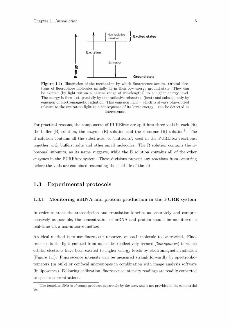
Figure 1.1: Illustration of the mechanism by which fluorescence occurs. Orbital elec-trons of fluorophore molecules initially lie in their low energy ground state. They canbe excited (by light within a narrow range of wavelengths) to a higher energy level.The energy is then lost, partially by non-radiative relaxation (heat) and subsequently byemission of electromagnetic radiation. This emission light – which is always blue-shiftedrelative to the excitation light as a consequence of its lower energy – can be detected as
fluorescence.
For practical reasons, the components of PUREfrex are split into three vials in each kit;
the buffer (B) solution, the enzyme (E) solution and the ribosome (R) solution2. The
B solution contains all the substrates, or ‘nutrients’, used in the PUREfrex reactions,
together with buffers, salts and other small molecules. The R solution contains the ri-
bosomal subunits, as its name suggests, while the E solution contains all of the other
enzymes in the PUREfrex system. These divisions prevent any reactions from occurring
before the vials are combined, extending the shelf life of the kit.
1.3 Experimental protocols
1.3.1 Monitoring mRNA and protein production in the PURE system
In order to track the transcription and translation kinetics as accurately and compre-
hensively as possible, the concentration of mRNA and protein should be monitored in
real-time via a non-invasive method.
An ideal method is to use fluorescent reporters on each molecule to be tracked. Fluo-
rescence is the light emitted from molecules (collectively termed fluorophores) in which
orbital electrons have been excited to higher energy levels by electromagnetic radiation
(Figure 1.1). Fluorescence intensity can be measured straightforwardly by spectropho-
tometers (in bulk) or confocal microscopes in combination with image analysis software
(in liposomes). Following calibration, fluorescence intensity readings are readily converted
to species concentrations.
2The template DNA is of course produced separately by the user, and is not provided in the commercialkit.

Chapter 1. Introduction 6
Figure 1.2: Schematic of the template DNA used to track both mRNA and proteinproduction in real time. As well as the YFP and Spinach coding sequences, the pro-moter, RBS, start/stop codons and T7 transcription terminator are also shown. A long(36 base-pair) linker sequence was used to increase the stability of the Spinach signal.Other features of the template DNA (including His and Xpress tags for protein detectionand purification) were neglected for clarity. Only the essential features relevant to the
discussions in this thesis have been included.
The wavelengths at which excitation and emission occur typically lie in relatively narrow
bandwidths, defining the excitation and emission spectra for each fluorophore. If multiple
fluorophores have distinct excitation and/or emission spectra, they can be imaged simulta-
neously when both excitation and emitted light are filtered and hence limited to a narrow
bandwidth3. If suitable distinct fluorophores are found for labelling both the mRNA and
protein produced in PUREfrex, then both transcription and translation kinetics can be
followed in real time.
Tracking protein production using this method is a standard procedure; green fluorescent
protein (GFP) has been used as a tracer molecule since 1995 and is now used ubiquitously
in molecular biology [17]. A wide range of variants with different excitation and emission
spectra have since been derived, allowing great flexibility in multi-species labelling [18].
If the template DNA used in a PUREfrex reaction codes for one of these GFP variants,
protein production kinetics can thus be monitored.
The mRNA molecule that would code for the fluorescent protein is not however itself
fluorescent. Instead, a so-called ‘Spinach’ sequence can be appended to the 3’ end of
the stop codon. This sequence folds into an aptamer that can bind a fluorophore called
DFHBI [19]. A particular property of DFHBI is that it only fluoresces if it is bound to a
correctly folded Spinach aptamer. The production of Spinach can thus also be monitored
in real time via fluorescence measurements.
In order to take advantage of these technologies, a template DNA sequence shown schemat-
ically in Figure 1.2 was used in PUREfrex reaction solutions. This method for simultane-
ous, real-time non-invasive tracking of protein and mRNA production has been validated
in both bulk and liposomal experiments [13]. For historical reasons, the GFP variant
chosen to track protein production was mEYFP (Monomeric Enhanced Yellow Fluores-
cent Protein). There is a degree of overlap between the mEYFP and Spinach spectra
(Figure 1.3) but with a judicious choice of excitation and emission light filters the degree
of crosstalk can be minimised (to be discussed further in Chapter 2).
3If there is a relatively small degree of overlap (or crosstalk) between the two spectra, they may alsobe imaged simultaneously but the detected signals would have to be corrected for crosstalk between thetwo fluorophores.
Chapter 1. Introduction 7
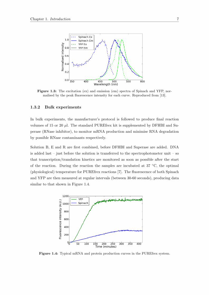
Figure 1.3: The excitation (ex) and emission (em) spectra of Spinach and YFP, nor-malised by the peak fluorescence intensity for each curve. Reproduced from [13].
1.3.2 Bulk experiments
In bulk experiments, the manufacturer’s protocol is followed to produce final reaction
volumes of 15 or 20 µl. The standard PUREfrex kit is supplemented by DFHBI and Su-
perase (RNase inhibitor), to monitor mRNA production and minimise RNA degradation
by possible RNase contaminants respectively.
Solution B, E and R are first combined, before DFHBI and Superase are added. DNA
is added last – just before the solution is transferred to the spectrophotometer unit – so
that transcription/translation kinetics are monitored as soon as possible after the start
of the reaction. During the reaction the samples are incubated at 37 ◦C, the optimal
(physiological) temperature for PUREfrex reactions [7]. The fluorescence of both Spinach
and YFP are then measured at regular intervals (between 30-60 seconds), producing data
similar to that shown in Figure 1.4.
Figure 1.4: Typical mRNA and protein production curves in the PUREfrex system.

Chapter 1. Introduction 8
These experiments will be referred to as kinetics experiments in the remainder of this
thesis. Attention should be drawn to the form of these curves. Protein production is
slightly delayed relative to mRNA production, but subsequently both species are produced
at a near-constant rate for several hours. The production of both YFP and Spinach then
stops rather abruptly, resulting in a horizontal fluorescence ‘plateau’ after ∼ 2.5−3 hours
of expression for YFP and ∼ 4.5−5 hours for Spinach. These features will become highly
relevant in the following chapters.
1.3.3 Liposome experiments
An illustration of the workflow for liposome experiments is shown in Figure 1.5. Firstly, a
mixture of lipids (DMPC/DMPG in the ratio 4/1, for this thesis) is labelled with TRITC
and PEG-biotin before being coated onto 200 µm glass beads. TRITC is a fluorophore
used to image the liposome membranes, while PEG-biotin acts to stabilise the vesicle and
allows it to bind to neutravidin and immobilise on the cover slip. An even coating is
achieved by organic solvent evaporation under continuous rotation in a round-bottomed
flask [10].
The lipids are then rehydrated in solution containing the template DNA as well as PURE-
frex solutions E and R. During the hydration process the lipids form membranes that
Figure 1.5: Workflow for liposome experiments. Lipids are first dehydrated (a) onto 200µm glass beads. They are then rehydrated (b) in a ‘swelling solution’ comtaining DNAand the E and R solutions from the PUREfrex system, to produce liposomes. These arethen transferred to a PDMS chamber on a cover slip (c) on which they are immobilised.PUREfrex B solution is then added to the external solution. After an incubation period(∼3 hours) at 37 ◦C the fluorescence produced during gene expression is imaged under a
confocal microscope. Reproduced from [10].
Chapter 1. Introduction 9
‘swell’ off the glass beads and encapsulate a portion of the solution (together with PURE-
frex reagents and DNA) in individual vesicles, or liposomes. Liposomes will also be inter-
changeably referred to as cells in this thesis.
A PDMS chamber is prepared on a glass cover slip to contain the liposomes for confocal
microscopy (Chapter 2.2). The base of the chamber is coated first in biotinylated bovine
serum albumen (BSA), which solidifies and immobilises a subsequent layer of neutravidin,
which binds to (multiple) biotin molecules. The liposome-containing solution is then
added, and biotin-labelled liposomes are bound to the fixed neutravidin molecules. Finally,
the PUREfrex B solution is added to the chamber. A portion of the small molecules and
tRNAs in the solution diffuses across the liposome membranes and permits gene expression
to occur intracellularly.
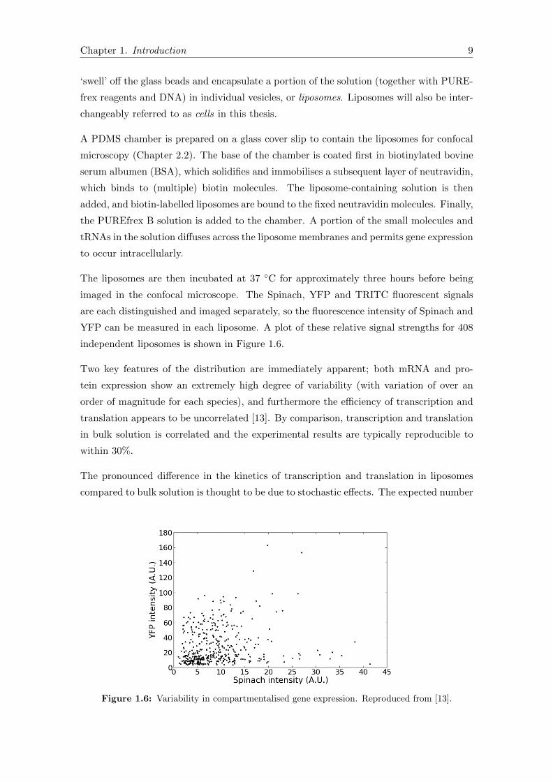
The liposomes are then incubated at 37 ◦C for approximately three hours before being
imaged in the confocal microscope. The Spinach, YFP and TRITC fluorescent signals
are each distinguished and imaged separately, so the fluorescence intensity of Spinach and
YFP can be measured in each liposome. A plot of these relative signal strengths for 408
independent liposomes is shown in Figure 1.6.
Two key features of the distribution are immediately apparent; both mRNA and pro-
tein expression show an extremely high degree of variability (with variation of over an
order of magnitude for each species), and furthermore the efficiency of transcription and
translation appears to be uncorrelated [13]. By comparison, transcription and translation
in bulk solution is correlated and the experimental results are typically reproducible to
within 30%.
The pronounced difference in the kinetics of transcription and translation in liposomes
compared to bulk solution is thought to be due to stochastic effects. The expected number
Figure 1.6: Variability in compartmentalised gene expression. Reproduced from [13].
Chapter 1. Introduction 10
of encapsulated molecules for some reagents in the liposomes4 are of order 1, and so
stochasticity in both reaction rates and encapsulation efficiency could be highly influential
on the system dynamics. The probability distributions governing these stochastic effects
are however as yet unknown.
1.4 Modelling techniques
A very useful approach to gain understanding about experimental systems – particularly
if they display surprising behaviour – is to model them mathematically. For this rea-
son, modelling will form the principal component of this thesis. A thorough theoretical
background to modelling techniques will be provided in the subsequent chapters; here we
shall restrict ourselves to a brief overview of the modelling philosophy adopted and the
techniques that were employed.
In the Danelon lab, the primary aim is to create a model capable of reproducing the salient
characteristics of both deterministic and stochastic mRNA and protein production, using
the PUREfrex expression platform under our particular experimental conditions. The
ambition is to create a model with minimal complexity that is still capable of reproducing
– and further, predicting – experimental results both in bulk and in liposomes, and which
can ultimately be extended to (multi-)gene networks. This is a long-term project that
began before the work presented in this thesis, and will also continue to develop in the
future [16, 20–22]. Approaches have varied significantly, from directly modelling almost
every elementary reaction in the PUREfrex system to phenomenological models that
focus on describing salient features of the observed behaviour instead of explaining their
microscopic origins. All of the previous work from the lab will be built on in this thesis with
the goal of developing a new, improved PUREfrex model with regard to the aims stated
above. In particular, for the first time the model will be tested not only deterministically,
but also using in-depth stochastic simulations to attempt to explain the distribution seen
in Figure 1.6.
In deterministic simulations, rate constants are fixed; rerunning the same simulation mul-
tiple times in a deterministic simulator will always yield the same results. In stochastic
simulators, the reaction rates are randomly drawn from a Poisson distribution (Appendix
A.1) where the mean is given by the fixed rate constant (which would normally be used
in a deterministic solver). The stochastic approach is fundamentally more accurate, since
the random distribution of molecular velocity and energy leads to stochasticity in the
rate of reactions. The time taken for reactant molecules to ‘find’ each other is described
by Brownian motion, and the chance of the molecules reacting upon collision depends
4based on the Poisson distribution, described in Appendix A.1.

Chapter 1. Introduction 11
on their energy and orientation at the time; all these factors have intrinsic randomness.
In a deterministic simulator only the average reaction rate is considered – this approx-
imation is only valid when copy numbers are large and/or reaction rates are relatively
fast, in which case the observed reaction rate is always averaged over a large number of
molecules. Since the deterministic approach is computationally far less intensive than
stochastic simulations, a deterministic model will be used to model gene expression in
bulk solution. Stochastic models will however be run to simulate liposomal conditions,
where low molecular copy numbers enhance the influence of stochastic effects.
Finally, an attempt will also be made to model the expression of self-regulated multi-
gene constructs in the PUREfrex system. Due to the added complexity introduced by
transcription factor binding and resource sharing between constructs – as well as account-
ing for the effects of supplementary enzymes in the reaction – the level of detail in the
model will be greatly reduced. The aim to reproduce existing experimental results and
inform future research directions will however still be pursued; a delicate balance between
simplicity and detail must be maintained to achieve this goal.
1.5 Research questions
The key research questions to be addressed in this thesis are:
• Can we make use of a microplate-reading (as opposed to cuvette-based) spectropho-
tometer to improve both the efficiency and reproducibility of PUREfrex bulk kinetics
experiments?
• Can we make use of a new in-house confocal microscope to image PUREfrex expres-
sion in liposomes?
• Is it possible to develop an improved model of PUREfrex gene expression that can
both fit and predict experimental results from bulk kinetics experiments, and con-
tains sufficient detail to be used in stochastic simulations without being prohibitively
computationally expensive?
• Are stochastic simulations (using the above model) able to inform possible causes
for the broad distribution of gene expression rates seen in Figure 1.6?
• Can a deterministic model for a multi-gene oscillating network suggest design prin-
ciples that may aid in understanding the system and improving its functionality?
These topics will be dealt with sequentially in the subsequent chapters, in the same order
that they appear in the above list.

Chapter 2
Development of experimental
techniques
This chapter covers a range of miscellaneous aspects of setting up two new instruments
for the purposes of research in the Danelon Lab. The Clariostar microplate reader was
primed for use to measure bulk PUREfrex kinetics experiments, while the Nikon confocal
microscope was employed for both visualising and quantifying PUREfrex expression in
liposomes.
2.1 Clariostar microplate reader for bulk experiments
2.1.1 Background and previous work
Originally, the kinetics of PUREfrex gene expression were measured in a cuvette-based
spectrophotometer (Cary Eclipse, Agilent Technologies). This meant that 20 µl of PURE
reaction mix had to be transferred into a cuvette before placement in the spectropho-
tometer (hereafter referred to as the ‘Eclipse’). Fluorescence readings of Spinach and
YFP signals were then collected via ’side-measurements’ through windows in the sides of
the cuvette (Figure 2.1).
There were numerous issues with this method of data collection which prompted the
lab to acquire a microplate reader (Clariostar, BMG Labtech) to perform fluorescence
measurements instead. Some of the key issues included:
• The process was relatively low throughput - only up to four experiments could be
performed in parallel, since only four cuvettes can be placed in the Eclipse at any
one time.
12

Chapter 2. Development of experimental techniques for improved data collection 13
Figure 2.1: Side-optic fluorescence measurement in the Eclipse cuvette-based spec-trophotometer. The excitation light passes through a transparent window in the side ofthe cuvette, and the emission light is collected on the opposite side (black arrow). Theheight of the solution (blue) is sufficient to cover the windows, and is far above the levelof the light path. An airtight lid (black) seals the cuvette to minimise evaporation. (Notto scale: the aspect ratio of the cuvette is much higher in reality, leading to a smaller
surface to volume ratio).
• Cuvettes are expensive and hence were reused between experiments. This had a
number of implications:
– The (micro-volume) cuvettes had to be cleaned very thoroughly to avoid con-
tamination between experiments, and the cleaning protocol was difficult and ex-
pensive to optimise [21]. Since fluorescence measurements were taken through
transparent windows in the cuvettes, these windows in particular had to be
cleaned very thoroughly between uses.
– The cleaning procedure was time-consuming, typically requiring 40 minutes for
a set of four cuvettes.
– The cleaning procedure involved vigorous drying steps using high-pressure ni-
trogen gas, which can introduce microscopic cracks in the glass cuvettes. These
cracks sometimes caused air bubbles to form during the kinetics measurements
(hypothesised to be due to the expansion of the trapped gas during incubation
at 37 ◦C), which led to irregularities in the fluorescence data as the bubble
passes the measurement windows.
– As a consequence of the above, fluorescence readings could sometimes exhibit
very high variability - up to 50% differences in final fluorescence intensities
were observed for identical reactions. This was largely attributed to insufficient
cleaning.
Using a microplate reader avoids the above issues because it is very high throughput
and no cleaning is necessary. Each microplate has 384 reaction wells that may be used
simultaneously, and they are economical enough for the wells not to be reused. Since the

Chapter 2. Development of experimental techniques for improved data collection 14
microplates are purchased sterile, they should remain clean as long as they are stored
appropriately before use.
Just van der Wolf, a former lab member, conducted investigations to determine a suit-
able protocol for using the microplate reader [21]. It was found that the most suitable
microplates for obtaining consistent fluorescence data had the following features:
• Black colour, to minimise background fluorescence;
• 20 µl well volumes, for 15 µl reaction volumes;
• Non-binding well coatings, that should prevent binding/immobilisation of the reac-
tion reagents/products on the well surfaces;
• Opaque black well bottoms, designed for top-optic fluorescence measurements;
• Clear adhesive plastic film ‘lids’, to cover the reaction wells both before and during
use in measurements.
Additionally, wells were pre-wetted with PURE buffer1 and subsequently emptied and
evaporated (at room temperature) for ∼15 minutes under the fume hood before samples
were pipetted into the wells. This procedure was found to improve the pipetting accuracy,
reducing interactions between the solutions and well surface.
A schematic of the experimental setup is illustrated in Figure 2.2.
Figure 2.2: Top-optic fluorescence measurements in the microplate reader. A cross-section of a single well is shown. The well is covered by a clear adhesive film to minimiseevaporation. The excitation light is shone on the sample, and the reflected emissionlight is collected in the detector. The angle between the excitation light beam and theorientation of the detector can be adjusted to focus on the surface of the sample, where
the maximum signal is expected.
1A solution prepared in the lab consisting of 50 mM HEPES, 100 mM potassium glutamate and 13mM magnesium acetate, designed to mimic the buffer conditions present in the PUREfrex solution.

Chapter 2. Development of experimental techniques for improved data collection 15
A particular issue that arose was that the fluorescence readings collected in the microplate
reader (hereafter referred to as the ‘Clariostar’) was highly sensitive to evaporation effects,
unlike the Eclipse. Since the reactions are incubated at 37 ◦C for several hours during
the kinetics measurements, some evaporation is expected to occur over this time period.
In a cuvette, the evaporation rate is lower than in a microplate due to the smaller surface
area/volume ratio of the solution. The cuvettes are also sealed with airtight lids, so after a
finite amount of evaporation has taken place a build-up of vapour pressure prevents further
(net) evaporation occurring. Moreover, the effect of evaporation is further minimised by
the fact that the fluorescence readings are taken via side-optic measurements (Figure
2.1). It is thus only noticeable if the bulk concentrations of the products (and/or reaction
components) are significantly increased by evaporation. As a consequence, evaporation
effects were found to be negligible in cuvettes for reactions lasting at least 5 hours2.
By contrast, the Clariostar makes top-optic fluorescence measurements. Excitation light
is shone on the surface of the sample, and the reflected emission light is detected (Figure
2.2). This approach is very sensitive to the height (and shape) of the surface of the sample,
and hence to evaporation. Microplate wells also have a relatively large surface/volume
ratio and do not usually have a lid, so the solutions they contain are more prone to
evaporation. Van der Wolf tested whether the addition of an oil layer over the reaction
solution would be sufficient to prevent evaporation, but unfortunately - although this
method did indeed prevent evaporation - it led to inconsistent fluorescence data. This
may be due to refraction of the excitation/emission light at the interface between the
two fluids and/or absorbance/fluorescence properties of the overlying oil itself. Small
differences in the quantity of oil added and the amount of mixing at the interface could
therefore cause substantial variability; these effects are avoided in cuvette measurements
because the light path does not cross the oil layer in the Eclipse.
Instead, use of the clear adhesive film mentioned above as a ‘well lid’ substantially reduced
evaporation and managed to maintain reasonably consistent fluorescence data. Residual
evaporation effects did however lead to a gradually decreasing fluorescence intensity over
time, which was clearly monitored using a solution of purified YFP 2.3. The formation
of condensation on the adhesive film, reducing its transparency, may have contributed to
this effect.
My aim was to further optimise Van der Wolf’s protocol for using the Clariostar to
obtain data to track PUREfrex gene expression kinetics. To this end, it was necessary to
quantitatively correct for the effect of evaporation on the raw data so that a meaningful
conversion from fluorescence intensity to Spinach/YFP concentrations could be developed.
2Consistent results were obtained over this time period in cuvettes both with and without a layer ofinert oil on top of the reaction solution.

Chapter 2. Development of experimental techniques for improved data collection 16
The hope was that use of the Clariostar would allow for reduced data variability as well
as efficient protocol execution.
In concrete, my key aims were to:
• Find methods to mitigate evaporation effects as much as possible, starting from Van
der Wolf’s protocol;
• Determine a suitable solution to use as a positive control to correct for evaporation
effects in kinetics measurement experiments;
• Determine a suitable solution to use as a negative control and correct for background
fluorescence;
• Determine suitable gain settings for the fluorescence detector to optimise the sig-
nal/noise ratio;
• Determine a calibration to convert arbitrary units of fluorescence to concentrations
of Spinach and YFP;
• Produce a set of PUREfrex kinetics data for a range of DNA concentrations that
can be used for model fitting.
The execution of the above aims is discussed in the following sections.
2.1.2 Determination and mitigation of evaporation effects
Identification of evaporation effects
The evaporation of sample solutions in the Clariostar was hypothesised to cause a drop
in detected fluorescence due either to the reduction in sample volume, condensation of
vapour on the well lids, or a combination of the two effects.
The measured fluorescence intensity reaches a peak when it is measured at the surface
of the solution, and decreases with distance away from the surface (Figure 2.4). The
measurement (focal) height should be located at the surface of the solution, since the
peak gives the ‘true’ fluorescence reading. The focal height is specified at the start of
the experiment, and remains fixed for the duration of the experiment. Thus, if over the
course of the experiment the surface level of the sample reduces due to evaporation, the
focal height would become increasingly distant from the focal height over time.
Condensation of water vapour on the well lids is caused by a difference in temperature
between the lid and the water vapour, and is also exacerbated by the fact that the lid

Chapter 2. Development of experimental techniques for improved data collection 17
Figure 2.3: Purified YFP fluorescence-time curve, exhibiting a 95% signal drop over1000 minutes in the Clariostar.
is adhesive, and hence vapour droplets have an increased tendency to stick to the lid.
This condensation causes light (both excitation and emission) to be scattered, and hence
reduces both the amount of fluorescence that is excited and the amount of fluorescence
that is detected over time.
To determine both the absolute and relative importance of the above two evaporation
effects, a sample of purified YFP was incubated at 37 ◦C in the microplate reader for
1000 minutes (16 hours 40 minutes) and the fluorescence was measured each minute.
YFP is fairly stable against spontaneous degradation, and since the sample was produced
in the PURExpress translation system, no protein degradation enzymes were present.
No measurable drop in fluorescence should therefore occur in the absence of evaporation
effects3.
It was found that up to 95% of the fluorescence appeared to be lost over 1000 minutes
of incubation (Figure 2.3), though this magnitude was highly variable between experi-
ments. A consistent observation was that most of the signal loss occurred at the start
of the experiment, and the loss rate decreased monotonically over time. This supports
the hypothesis that the signal drop is an evaporation effect, since most evaporation is
expected to occur at the initial phase of the experiment, when the solution is heating
up and the vapour pressure is low. As time passes, the sample solution equilibrates at
the incubation temperature and the vapour pressure increases until (theoretically, in a
perfectly sealed well with inert surfaces) no more evaporation occurs (Appendix ??). The
continued (if gradual) signal drop over time may be due to imperfect well sealing and/or
the adhesiveness of the well lid driving the evaporation reaction forward.
3No drop in fluorescence is observed when the same experiment is performed using cuvettes in theEclipse, which supports this statement.
Chapter 2. Development of experimental techniques for improved data collection 18
8 9 10 11 12 13 14 15Focalyheight y(m m )
0.0
0.2
0.4
0.6
0.8
1.0
Re
lati
ve
yflu
ore
sce
nce
yin
ten
sity
y(A
.U.)
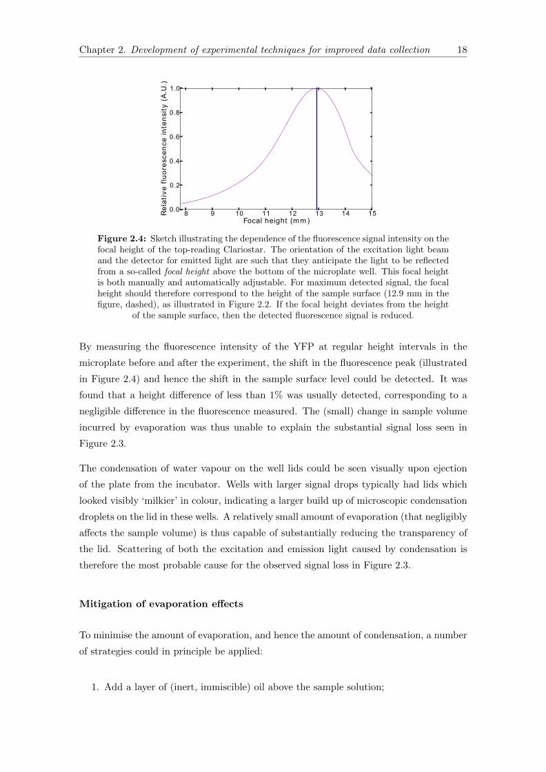
Figure 2.4: Sketch illustrating the dependence of the fluorescence signal intensity on thefocal height of the top-reading Clariostar. The orientation of the excitation light beamand the detector for emitted light are such that they anticipate the light to be reflectedfrom a so-called focal height above the bottom of the microplate well. This focal heightis both manually and automatically adjustable. For maximum detected signal, the focalheight should therefore correspond to the height of the sample surface (12.9 mm in thefigure, dashed), as illustrated in Figure 2.2. If the focal height deviates from the height
of the sample surface, then the detected fluorescence signal is reduced.
By measuring the fluorescence intensity of the YFP at regular height intervals in the
microplate before and after the experiment, the shift in the fluorescence peak (illustrated
in Figure 2.4) and hence the shift in the sample surface level could be detected. It was
found that a height difference of less than 1% was usually detected, corresponding to a
negligible difference in the fluorescence measured. The (small) change in sample volume
incurred by evaporation was thus unable to explain the substantial signal loss seen in
Figure 2.3.
The condensation of water vapour on the well lids could be seen visually upon ejection
of the plate from the incubator. Wells with larger signal drops typically had lids which
looked visibly ‘milkier’ in colour, indicating a larger build up of microscopic condensation
droplets on the lid in these wells. A relatively small amount of evaporation (that negligibly
affects the sample volume) is thus capable of substantially reducing the transparency of
the lid. Scattering of both the excitation and emission light caused by condensation is
therefore the most probable cause for the observed signal loss in Figure 2.3.
Mitigation of evaporation effects
To minimise the amount of evaporation, and hence the amount of condensation, a number
of strategies could in principle be applied:
1. Add a layer of (inert, immiscible) oil above the sample solution;
Chapter 2. Development of experimental techniques for improved data collection 19
2. Apply a vertical temperature gradient to the wells, such that the well lid is at a
higher temperature than the sample;
3. Reduce the incubation temperature;
4. Avoid using wells in the outer rows/columns of each microplate;
5. Improved well sealing;
6. Reduce sample surface/volume ratio in wells.
Not all strategies can be straightforwardly applied in practice, however. Adding a layer of
oil, for instance, introduced a substantial amount of variability in the fluorescence readings
[21], as discussed above. Further, it was not possible to apply a vertical temperature
gradient in the Clariostar microplate reader, though this feature is available on some other
models (such as Bioscreen C MBR, Oy Growth Curves Ab Ltd). Additionally, varying
the incubation temperature can significantly affect gene expression kinetics [10, 22]; it is
thus not an independent parameter that can be varied to improve the accuracy of kinetics
measurements. The effect of temperature adjustment on evaporation therefore was not
investigated here.
Only the final three points in the above list were therefore studied. The fourth point
relates to what is commonly termed the ‘edge-effect’ in microplates; when microplates
are incubated at elevated temperatures, wells on the periphery typically exhibit enhanced
evaporation relative to the central wells [23]. This may be due to uneven heating in
microplate readers. Consequently, the outer three rows/columns in each plate were not
used in any of the experiments described in this thesis, and variations in evaporation
patterns were not detected in the remaining inner wells.
Since the well lids currently used in the lab are adhesive films, optimal sealing can be
achieved by maintaining a clean microplate (dust-free) and by pressing the film as firmly as
possible around the rim of each well. It was found that once a new package of microplates
was opened, simply storing the unused microplates in a loosely sealed plastic bag was
insufficient to keep them dust-free; the measured fluorescence from an incubated sample
of purified YFP in such a stored microplate showed a much larger signal drop over time
than when using a new microplate from an unopened package. To maintain opened
but unused microplates in a cleaner condition, new packages were opened upside down
under the fume hood, (so only the base of the unused microplates are exposed when the
package is opened) and the microplate to be used is covered by a sheet of adhesive film.
This prevents dust from gathering on unused wells before they are utilised (only a small
portion of the microplate is typically used for each set of experiments). For each new
experiment, the portion of film covering the number of wells to be used (as well as a

Chapter 2. Development of experimental techniques for improved data collection 20
Figure 2.5: Microplate film cutting arrangement. First, the entire microplate is coveredin adhesive plastic film (light grey). A section is then cut out with a scalpel, exposingthe wells to be used in experiments (blue) as well as all the peripheral wells. A freshplastic film is then applied to cover the inner wells. This arrangement ensures that thereis enough room to achieve a tight sealing on the inner wells, without hindrance from thesurrounding film. (Note: the number of wells has been reduced in this illustration for
clarity.)
peripheral border, Figure 2.5) is cut out with a scalpel and discarded. A new portion
of film large enough to cover the used wells and their peripheral border is then firmly
stuck to the plate using a clean flat edge to firmly press the film with a ‘sweeping’ motion
over the plate. Using this method, the amount of evaporation was minimised (the drop
in fluorescence of purified YFP after the incubation period was substantially reduced, as
was the ‘milkiness’ of the well lids).
To further reduce evaporation effects, it may be possible to purchase microplates and lids
which are better designed to minimise evaporation. For instance, microplates with taller,
narrower wells reduce the surface/volume ratio of the sample solution and hence reduce
the rate of evaporation. Microplates without a raised rim (present on the lab microplates)
also give a larger surface area to securely seal the adhesive film lids. Some alternative
microplate lids also offer different sealing methods (so they are no longer adhesive, but
simply fit snugly on the wells) and can even be pre-humidified to increase the vapour
pressure and reduce evaporation of the sample.
After researching various products available, it was found that pre-humidifying microplate
lids (such as Labcyte MicroClimer Environmental Lids, cat. no. LLS-0310-IP) are not
completely transparent, and would therefore introduce an additional source of variability
in fluorescence measurements. Non-adhesive microplate lids (such as Evergreen Scientific
cat. no. 290-8219-03L) also cannot usually be cut to cover only a few wells at a time;
the whole lid must be used for tight sealing on a microplate. Given that in a typical
PUREfrex experiment less than 10 out of 384 wells in a microplate are used, it would be
rather wasteful to use a full microplate lid for each experiment.
Chapter 2. Development of experimental techniques for improved data collection 21
Microplates without a raised rim are also hard to come by, because raised rims are consid-
ered useful to avoid cross-contamination between wells [24] – this is a valued feature for
most microplate applications, though it is not an issue for PUREfrex kinetics experiments.
It was not possible to find flat-rimmed microplates that match all other specifications nec-
essary for our experiments (listed in section 2.1.1).
Microplates with smaller surface/volume ratios were found (Corning, cat. no. 3728),
however the narrower well diameter could potentially make pipetting the sample into the
wells significantly more difficult. A sample of these microplates were thus ordered, but
they have not yet been tested. For the purposes of this project the evaporation effect
was reasonably well corrected for using a positive control and the evaporation mitigation
measures described above using the original microplate/lid combination. It may how-
ever be worthwhile to test these alternative microplates in the future if under certain
circumstances evaporation becomes a more significant issue.
2.1.3 Determination of appropriate control samples
Although the effects of evaporation could be mitigated significantly using techniques de-
scribed in the previous section, the drop in fluorescence for a sample of purified YFP was
still non-negligible – up to 60% of the signal could be lost over 1000 minutes. This meant
that the fluorescence data collected from the Clariostar could not be taken at face value;
the effect of evaporation would have to be corrected for somehow.
Naively, it may be assumed that the fractional signal drop for purified YFP may match
the signal drop for PUREfrex kinetics samples, and thus by correcting the kinetics data
with the signal drop detected over the same time period using purified YFP (thus using
it as a ‘positive control’) the true fluorescence signal may be recovered. However, it was
found that the signal drop for purified YFP was much greater than that shown by YFP
in PUREfrex kinetics experiments in the Clariostar. In PUREfrex experiments, the drop
seen in the signal curves for YFP fluorescence after the protein plateau was typically
around 5% per hour, whereas a drop of 10% per hour was typical for purified YFP. This
difference may be due to the high concentration of solutes in the PUREfrex solution –
absent in the purified YFP sample – which may affect the evaporation dynamics of the
solution. Furthermore, the signal drop for Spinach and YFP fluorescence may be different,
but no distinction is made for the two channels if only purified YFP is used as a positive
control.
An alternative positive control would be a non-purified sample of YFP and Spinach pro-
duced in the PUREfrex system, where gene expression was run for long enough that both

Chapter 2. Development of experimental techniques for improved data collection 22
Figure 2.6: Spinach and YFP kinetics data, before and after correcting for evaporationeffects. For these data, the reference timepoint chosen to calculate fractional signal loss
in the positive control was at 60 minutes.
protein and mRNA plateaus have been reached and hence no production (and little degra-
dation) is expected. In such a sample (hereafter referred to as a ‘plateaued PUREfrex
solution’), the effect of evaporation on both the YFP and Spinach fluorescence channels
are tracked, and the solution conditions represent those found in the experimental samples
more closely. Correcting experimental data by assuming the same fractional fluorescence
loss as that detected in the positive control sample was shown to be quite effective; the
distinctive horizontal protein plateau was recovered, for example (Figure 2.6).
The Spinach plateau was not horizontal after the correction, but instead had a negative
gradient. This may be explained by (spontaneous) mRNA degradation, for which there
has been some evidence from Eclipse kinetics measurements as well4.
A negative control solution was necessary to account for the background fluorescence that
must be subtracted for each fluorescence channel. Two options were tested: MilliQ pure
water, and the PUREfrex reaction mixture in the absence of DNA (so no YFP or Spinach
would be produced). Technically, the latter option is the more appropriate negative
control since it accounts for background fluorescence produced by any other reagents in
the PUREfrex system, as well as that produced by water. However it was found that
there was a negligible difference in fluorescence measured from either option.
At least, this was the case for the first hour or so of the incubation time. The MilliQ
sample, similar to the purified YFP sample, was particularly prone to evaporation and
after some hours even formed macroscopic condensation droplets on the well lid. The
effect of evaporation was noticeable within the first hour of incubation; the ‘background’
4Though not for the first 3 hours of expression [13].

Chapter 2. Development of experimental techniques for improved data collection 23
signal in the Spinach channel began to increase over time, for example, where it would
normally be expected to stay constant. The DNA-free PUREfrex solution, which does not
suffer from enhanced evaporation relative to standard PUREfrex reaction samples, indeed
shows a constant background signal. Interestingly, this indicates that the background
fluorescence is affected very differently by evaporation compared to either YFP or Spinach,
and so should not be corrected for evaporation effects in the same way.
Since MilliQ is far more economical to use as a negative control than DNA-free PUREfrex
solution, and given that the two samples (initially) give very similar background fluores-
cence values, it was decided to use MilliQ as a negative control. To avoid evaporation
effects a time-average was taken using 15 consecutive fluorescence readings between 20-35
minutes after the start of incubation (at which point the sample is assumed to have equi-
librated to the incubation temperature, but evaporation effects are not yet noticeable).
The overall formula applied to process the raw data into the corrected form using the
positive and negative controls is as follows:
xt,c = (xt,r − n)(pt1 − n)
(pt − n)(2.1)
where xt,c is the evaporation-corrected and background-corrected sample fluorescence at
time t, xt,r is the raw sample data at time t, n is the averaged background fluorescence
measured in the negative control, pt1 is the fluorescence measured in the positive control at
a reference timepoint t1 (which should be the timepoint chosen to make the fluorescence-
concentration calibration, described in section 2.1.5) and pt is the fluorescence in the
positive control at time t. xt,c therefore corresponds to the Spinach/YFP fluorescence
that would have been measured if the influence of evaporation at time t was equal to that
at time t1.
2.1.4 Determination of appropriate gain settings
Before a fluorescence signal reaches the detector in the plate reader, the light first passes
through a photomultiplier tube (PMT) in which the signal is amplified. This amplifica-
tion process is designed to increase the fluorescent signal more than the accompanying
noise, and hence improve the signal/noise ratio in the measurement. There is however a
maximum signal that can be registered by the detector, so there is a limit to how high
the signal can be amplified before it saturates.
The amount by which the signal is amplified can be controlled by varying the ‘gain’ setting
of the device. In principle, to maximise the signal/noise ratio the gain should be set as

Chapter 2. Development of experimental techniques for improved data collection 24
Figure 2.7: Signal-gain relationship for Spinach and YFP in the Clariostar. A sampleof plateaued PUREfrex solution containing 0.74 nM DNA was used to gather these data.
The final chosen gain (2000) is indicated by the dashed line.
high as possible without saturating the signal. The gain can also be adjusted separately
for different fluorescence channels.
To select an appropriate gain setting for the YFP and Spinach channels, the signal-gain
relationship was plotted for a sample of plateaued PUREfrex solution containing 0.74 nM
DNA (Figure 2.7). The maximum detectable signal is 250,000 AU, so in principle the
best gain settings for an optimal signal/noise ratio are approximately 2900 for Spinach
and 2650 for YFP in this sample.
However, in order to be able to use a single fluorescence-to-concentration calibration for
all PUREfrex (and, ideally, PURExpress) kinetics measurements in the Clariostar, it
would be most convenient to choose gain settings that are appropriate for a wide range
of DNA concentrations. PURExpress has been found to produce approximately eight
times more protein than PUREfrex, and the Spinach yield was also known to increase
with DNA concentrations above 0.74 nM [25]. Since the fluorescence signals should scale
linearly with species concentration (discussed further in the next section), a gain of 2000
was chosen for both the Spinach and YFP channels. An eight-fold increase in YFP and
Spinach concentrations could then still be measured using the same gain settings without
saturating the signal.
These settings were still found to have an acceptable signal/noise ratio for the test sample
– background fluorescence measured using a MilliQ sample was 8% and 2% of the signal
in the Spinach and YFP channels respectively, and the size of signal fluctuations were
less than 1% of the signal strength at the plateau level. These fluctuations are negligible
compared to the magnitude of experimental errors (discussed further in section 2.1.6).
It should also be mentioned that the degree of crosstalk (undesirable signal produced by
each fluorophore in fluorescence channels other than their own) in the Clariostar was very
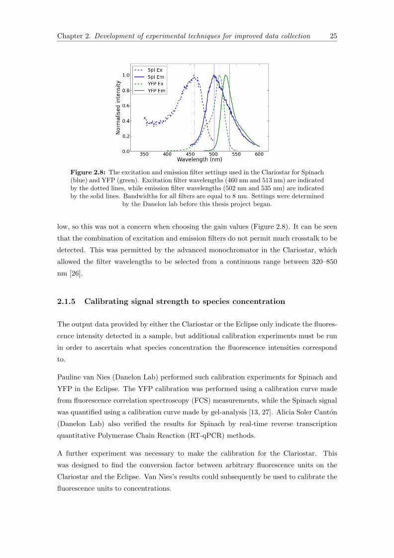
Chapter 2. Development of experimental techniques for improved data collection 25
Figure 2.8: The excitation and emission filter settings used in the Clariostar for Spinach(blue) and YFP (green). Excitation filter wavelengths (460 nm and 513 nm) are indicatedby the dotted lines, while emission filter wavelengths (502 nm and 535 nm) are indicatedby the solid lines. Bandwidths for all filters are equal to 8 nm. Settings were determined
by the Danelon lab before this thesis project began.
low, so this was not a concern when choosing the gain values (Figure 2.8). It can be seen
that the combination of excitation and emission filters do not permit much crosstalk to be
detected. This was permitted by the advanced monochromator in the Clariostar, which
allowed the filter wavelengths to be selected from a continuous range between 320–850
nm [26].
2.1.5 Calibrating signal strength to species concentration
The output data provided by either the Clariostar or the Eclipse only indicate the fluores-
cence intensity detected in a sample, but additional calibration experiments must be run
in order to ascertain what species concentration the fluorescence intensities correspond
to.
Pauline van Nies (Danelon Lab) performed such calibration experiments for Spinach and
YFP in the Eclipse. The YFP calibration was performed using a calibration curve made
from fluorescence correlation spectroscopy (FCS) measurements, while the Spinach signal
was quantified using a calibration curve made by gel-analysis [13, 27]. Alicia Soler Canton
(Danelon Lab) also verified the results for Spinach by real-time reverse transcription
quantitative Polymerase Chain Reaction (RT-qPCR) methods.
A further experiment was necessary to make the calibration for the Clariostar. This
was designed to find the conversion factor between arbitrary fluorescence units on the
Clariostar and the Eclipse. Van Nies’s results could subsequently be used to calibrate the
fluorescence units to concentrations.

Chapter 2. Development of experimental techniques for improved data collection 26
Figure 2.9: Calibration curve for Clariostar and Eclipse fluorescence readings. The threesamples contained 33%, 67% and 100% plateaued PUREfrex solution, where dilutionswere performed using MilliQ. Best-fit lines have equations y = 142x and y = 1016x forthe Spinach and YFP curves respectively. Eclipse readings were taken using high andmedium gain for Spinach and YFP (respectively), while Clariostar readings were taken
as described in the main text.
A sample of plateaued PUREfrex solution was made in three dilutions; namely in ra-
tios of 1:2, 2:1 and 1:0 to MilliQ. The Spinach and YFP signals for these samples were
then measured, together with a MilliQ blank solution, for two hours in the Clariostar.
It was decided to use the measurements taken at 1 hour for the calibration, at which
point evaporation effects had stabilised to a smooth curve that was reproducible between
experiments. For this purpose, the consecutive readings taken at 59, 60 and 61 minutes
were averaged, and the background fluorescence measured from the MilliQ sample was
subtracted. As previously discussed, the measured fluorescence is strongly time depen-
dent, so the timepoint chosen to make the calibration would decide the reference point
used for making evaporation corrections (t1 in equation 2.1).
After the measurement in the Clariostar, the three samples were transferred to cuvettes to
be measured in the Eclipse using identical settings to those used by Van Nies for the con-
centration calibration. Since these measurements are not affected by evaporation effects,
the readings (taken every 30 seconds) became roughly constant after just two minutes of
incubation. An average of the readings taken between 10-20 minutes of incubation was
used as the final measurement for each sample.
Finally, the data was used to make a calibration curve to compare fluorescence mea-
surements on the Clariostar with those on the Eclipse (Figure 2.9). The background
fluorescence measured on the Eclipse was found to be negligible, so a linear fitting was
made that was fixed to pass through the origin (effectively treating it as a fourth data
point).

Chapter 2. Development of experimental techniques for improved data collection 27
The data points are separated by regular intervals, confirming that the fluorescence sig-
nal increases linearly with Spinach/YFP concentration. The gradient of the fitted line
therefore gives the conversion factor between the measurement settings on the two ma-
chines; 142 A.U. on the Clariostar corresponds to 1 A.U. on the Eclipse with high gain
for Spinach, and 1016 A.U. on the Clariostar corresponds to 1 A.U. on the Eclipse with
medium gain for YFP. The high R2 value for the fitting (0.984 for Spinach, 0.995 for
YFP) indicate that the fitting has a high confidence level; there is a < 2% deviation from
the trend, which can be associated with intrinsic variability.
Using Van Nies’s calibration, therefore, a calibration of (0.070 ± 0.015) nM/A.U. and
(4.5±0.28)×10−3 nM/A.U. is obtained on the Clariostar for Spinach and YFP respectively.
Caution must be taken when using these values, however; they apply only if a gain of 2000
is used for both Spinach and YFP channels, and if the microplate is incubated at 37 ◦C. A
new calibration must be made if either of these conditions are changed. Furthermore, the
experiment must last at least one hour, starting from the moment the plate is placed in
the incubator, in order to use the correct reference timepoint (60 minutes) when making
the evaporation correction to the experimental data (equation 2.1).
2.1.6 Acquiring model-fitting kinetics data
An important aim of this project was to validate the model of PUREfrex gene expression
over a wide range of DNA concentrations. It was therefore decided to produce kinetics
data using DNA concentrations ranging from 0.2 nM to 20 nM, thus encompassing two
orders of magnitude. These data would be collected in the Clariostar, using the sam-
ple/well preparation protocol by Just van der Wolf [21] in conjunction with the additional
precautions, settings and data processing steps described earlier in this chapter.
Previous work in the lab by Roeland van Wijk had indicated that DNA saturates the
PUREfrex transcription machinery at a concentration of between 7 nM and 14 nM [25].
Since the most interesting variation in kinetics would thus occur at lower DNA concen-
trations, the final concentrations chosen to run the experiments were 0.2 nM, 1 nM, 5
nM and 20 nM. This data would be supplemented by recent kinetics experiments run by
Pauline van Nies at 0.74 nM and 7.4 nM DNA concentrations.
Furthermore, in order to test and account for variability in the kinetics measurements, re-
peat experiments were made at each of the chosen DNA concentrations. These repeats had
two forms; one in which a single ‘double-portion’ of PUREfrex reaction mix was produced
and divided between two wells, and one in which the entire PUREfrex reaction mixture
was produced separately for each repeat. The first form (known as a duplo experiment)
therefore mainly quantifies the variability inherent in the measuring instrument. In the

Chapter 2. Development of experimental techniques for improved data collection 28
Figure 2.10: Comparison of two duplo experiments (labelled 1 and 2), for Spinach(blue) and YFP (green) signals. A DNA concentration of 20 nM was used, and the datahas been corrected for both evaporation and background fluorescence as described in
section 2.1.3.
case of the Clariostar, this accounts for artefacts introduced by inhomogeneities in the
well lids, variability in condensation formation, and differences in the sample meniscus
curvature, among others. The second form gives the more complete picture of experi-
mental variability, accounting for that incurred by sample preparation and measurement
method combined.
It was found that in duplo experiments the variability was typically less than 20%, and
the fluorescence curves looked almost identical apart from this scaling - the expression
time for example is identical for each duplo (Figure 2.10). This is expected for variability
associated solely with the measuring instrument; since the ratio of all reagents are identical
for each repeat, the real dynamics of the system should be identical. Variability in the
measurement would typically affect all fluorescence readings by the same proportion (for
example, if one well lid is slightly cleaner than the other, then a higher fluorescence reading
would be consistently expected), and hence result in one dataset being simply a ‘scaled’
version of the other in a duplo.
However, when a kinetics experiment was completely repeated on a separate day, not
only the magnitude of the fluorescence reading but also the expression time showed some
variability. This may be due to pipetting errors, which can lead to differences in the
reagent concentrations between the two repeats and can be enough to cause detectable
differences in the system dynamics. More surprisingly, the variability in fluorescence
intensity ranged up to 50% while expression times tended to remain consistent within a
10% range (Figure 2.11). This difference led to the suspicion that the large disparity in
fluorescence intensity may be yet another instrument-related artefact.
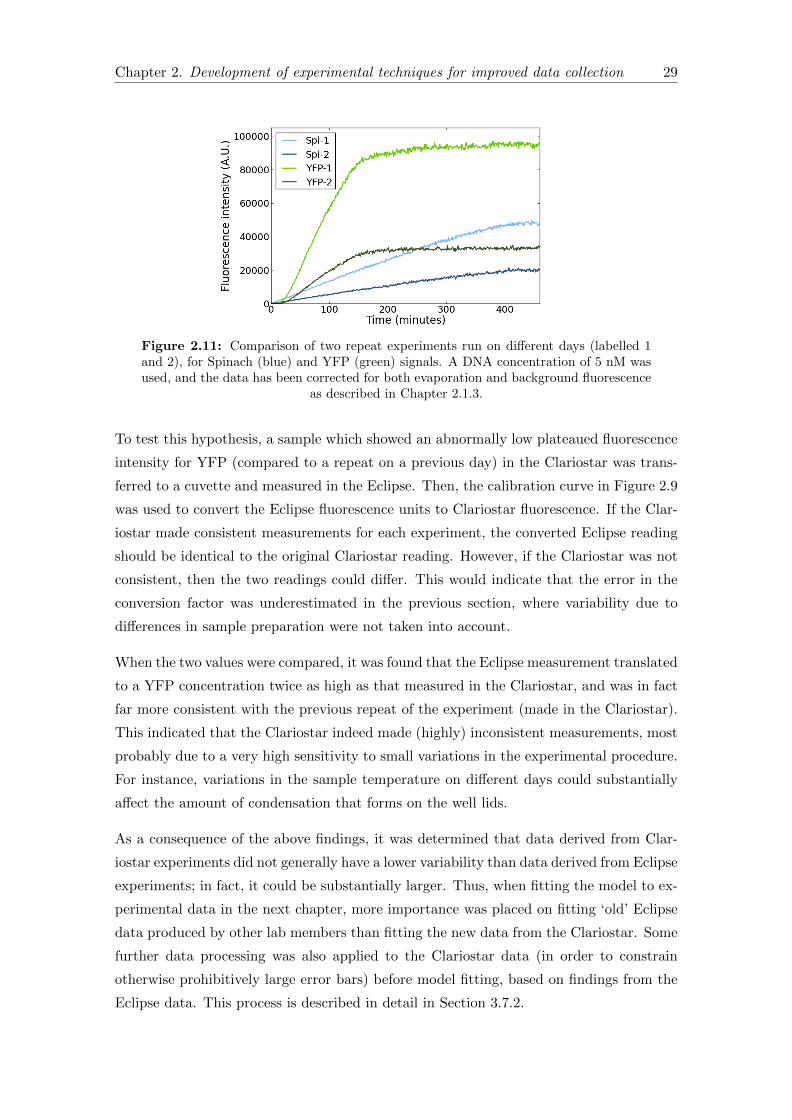
Chapter 2. Development of experimental techniques for improved data collection 29
Figure 2.11: Comparison of two repeat experiments run on different days (labelled 1and 2), for Spinach (blue) and YFP (green) signals. A DNA concentration of 5 nM wasused, and the data has been corrected for both evaporation and background fluorescence
as described in Chapter 2.1.3.
To test this hypothesis, a sample which showed an abnormally low plateaued fluorescence
intensity for YFP (compared to a repeat on a previous day) in the Clariostar was trans-
ferred to a cuvette and measured in the Eclipse. Then, the calibration curve in Figure 2.9
was used to convert the Eclipse fluorescence units to Clariostar fluorescence. If the Clar-
iostar made consistent measurements for each experiment, the converted Eclipse reading
should be identical to the original Clariostar reading. However, if the Clariostar was not
consistent, then the two readings could differ. This would indicate that the error in the
conversion factor was underestimated in the previous section, where variability due to
differences in sample preparation were not taken into account.
When the two values were compared, it was found that the Eclipse measurement translated
to a YFP concentration twice as high as that measured in the Clariostar, and was in fact
far more consistent with the previous repeat of the experiment (made in the Clariostar).
This indicated that the Clariostar indeed made (highly) inconsistent measurements, most
probably due to a very high sensitivity to small variations in the experimental procedure.
For instance, variations in the sample temperature on different days could substantially
affect the amount of condensation that forms on the well lids.
As a consequence of the above findings, it was determined that data derived from Clar-
iostar experiments did not generally have a lower variability than data derived from Eclipse
experiments; in fact, it could be substantially larger. Thus, when fitting the model to ex-
perimental data in the next chapter, more importance was placed on fitting ‘old’ Eclipse
data produced by other lab members than fitting the new data from the Clariostar. Some
further data processing was also applied to the Clariostar data (in order to constrain
otherwise prohibitively large error bars) before model fitting, based on findings from the
Eclipse data. This process is described in detail in Section 3.7.2.

Chapter 2. Development of experimental techniques for improved data collection 30
2.1.7 Summary and recommendations
Unfortunately, in order to extract accurate quantitative information from the Clariostar
the raw data must be processed quite substantially. Corrections must be made to account
for evaporation effects (attributed to condensation formation on well lids) as well as
background fluorescence. Additionally, although a calibration of fluorescence intensity to
species concentration has been performed, its reliability is dubious. This is because a
large variability (of up to 50%) between repeat experiments suggests that the instrument
is very sensitive to small differences in the sample preparation protocol; the amount of
condensation formation may vary substantially depending on the sample temperature
pre-incubation, for example. The degree of variability also means that the quality of the
data is poor for model-fitting purposes; further processing (to be discussed in Chapter
3.7.2) is necessary to make it usable, at which point the validity of the data may be called
into question. Furthermore, the time spent on data processing could easily exceed the
extra time that it might have taken to perform the same experiments on the Eclipse,
negating the efficiency benefit of using the Clariostar. It is therefore not advisable to use
the Clariostar instead of the Eclipse for any incubated kinetics experiments from which
accurate quantitative data is desired.
The Clariostar is however suitable for performing experiments where qualitative features
are of more interest; for instance, checking whether it is possible to restart translation
after the protein plateau is reached (section 3.5.2). It may also be appropriate for running
kinetics expression at room temperature, in which case well lids would not be necessary
and so neither evaporation, condensation nor film heterogeneity effects would affect the
data. In these situations, the Clariostar is an adequate instrument for monitoring PURE-
frex kinetics experiments in an efficient and straightforward manner. Unlike the Eclipse,
no tedious cleaning procedure was required and an effectively unlimited number of ex-
periments could be run in parallel, if desired. A thorough protocol was developed that
accounted for various nuances in the operation of the instrument, mitigating evaporation
as much as possible and selecting appropriate gain settings to optimise the signal/noise
ratio. The gain was also specially chosen to avoid oversaturating the detector in either
PUREfrex or PURExpress experiments, so the settings may be used by default for any
future investigations.
Some suggestions for further work include:
• Investigate the use of smaller wells with a lower surface area/volume ratio, where
the evaporation rate is expected to be lower.
Chapter 2. Development of experimental techniques for improved data collection 31
• Investigate use of the Clariostar for kinetics experiments run at lower temperatures.
Below a certain temperature, the amount of evaporation may reduce to the point
that condensation effects are minimal.
• Run some repeated kinetics experiments at room temperature without the well lids.
Any variability seen in these experiments could not be associated to evaporation
effects in any regard. Differences in the level of variability between these experiments
and those described in section 2.1.5 can be ascribed specifically to evaporation effects
and those due to the presence of a well lid.
These experiments could help both to understand and remedy the causes for the issues
described earlier in the chapter.
2.2 Nikon confocal microscope for liposome experiments
Use of either a plate reader or cuvette spectrophotometer is only suitable for measuring
bulk gene expression, in free solution. The resolution and specificity required to measure
compartmentalised gene expression in a solution of liposomes can only be obtained by
fluorescence microscopy.
To date, a Zeiss LSM710 laser scanning confocal microscope, located in the Department
of Chemical Engineering at TU Delft, has been used by the Danelon lab for imaging gene
expression in liposomes. Recently, a Nikon A1R laser scanning confocal microscope has
been installed in the Bionanoscience Department. The new microscope also interfaces with
a Nikon N-SIM structured illumination microscope (SIM), which is capable of imaging at a
substantially higher resolution than a standard light microscope. Nikon image acquisition
and analysis software (NIS- Elements Advanced Research) is also integrated and capable
of more advanced and more straightforward image processing than the built-in software
available using the Zeiss [28].
It would be far more convenient for the lab to use the new in-house microscope to avoid
the need to transport samples between the two departments for imaging. The advanced
software can also save time during image processing (measuring liposome sizes and mean
fluorescence intensities in a population of liposomes). Use of the SIM could also permit
smaller liposomes to be studied than before. However, tests must first be run to check
that the quality of images produced using the Nikon system are sufficient to accurately
measure fluorescence intensity from liposomes; issues may be caused by image blur or low
signal/noise ratio, for example.
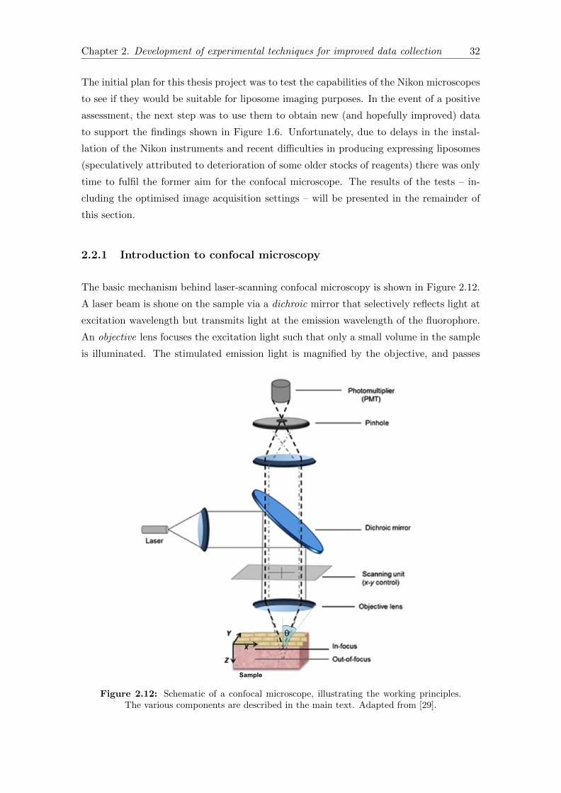
Chapter 2. Development of experimental techniques for improved data collection 32
The initial plan for this thesis project was to test the capabilities of the Nikon microscopes
to see if they would be suitable for liposome imaging purposes. In the event of a positive
assessment, the next step was to use them to obtain new (and hopefully improved) data
to support the findings shown in Figure 1.6. Unfortunately, due to delays in the instal-
lation of the Nikon instruments and recent difficulties in producing expressing liposomes
(speculatively attributed to deterioration of some older stocks of reagents) there was only
time to fulfil the former aim for the confocal microscope. The results of the tests – in-
cluding the optimised image acquisition settings – will be presented in the remainder of
this section.
2.2.1 Introduction to confocal microscopy
The basic mechanism behind laser-scanning confocal microscopy is shown in Figure 2.12.
A laser beam is shone on the sample via a dichroic mirror that selectively reflects light at
excitation wavelength but transmits light at the emission wavelength of the fluorophore.
An objective lens focuses the excitation light such that only a small volume in the sample
is illuminated. The stimulated emission light is magnified by the objective, and passes
Figure 2.12: Schematic of a confocal microscope, illustrating the working principles.The various components are described in the main text. Adapted from [29].
Chapter 2. Development of experimental techniques for improved data collection 33
through the dichroic mirror and into a photomultiplier tube (PMT). The function of the
PMT is two-fold; firstly it eliminate background signal below a specified threshold, and
secondly it amplifies the remaining signal by a multiplicative factor. The threshold can
be adjusted by varying the user-defined offset and the factor is controlled by the user-
specified gain. Once the emission light passes through the PMT it reaches the photo-
detector, where it is transduced into an electrical signal and quantified. By scanning the
excitation laser point-by-point over the sample (pausing at each point for a given dwell
time to collect data) an image of the full focal plane is constructed. Movement of the
sample in the z-direction (also termed the axial direction) allows multiple optical slices
to be imaged in this way, and can thus permit the reconstruction of 3D images.
To improve the signal-to-noise ratio, the emission light is also spatially filtered by a pinhole
aperture before it reaches the photodetector. The pinhole removes out-of-focus light and
ensures that the detected photons are sourced only from a very small confocal volume in
the sample around the focal point. The size of this volume determines the resolution of
the final image and may be controlled by adjusting the pinhole size. It is also diffraction-
limited; it is not possible for the confocal volume to reduce below a wavelength- and
material-dependent minimum value, regardless of the pinhole size.
The diffraction limit is a fundamental physical property of light. Due to diffraction, the
radius r of the smallest point to which light can be focused by a perfect lens is given by:
r =λ
2nsinθ(2.2)
where λ is the wavelength, n is the refractive index of the medium between the lens and
the focal point and θ is the half-angle defined by the edge of the lens and the focal point,
shown in Figure 2.12 [30]. The disk with radius r is known as the Airy disk, and gives
the minimum pixel size in a confocal image. 2r defines an Airy unit, which is often used
to measure confocal pinhole diameters (see section 2.2.2.2).
The product nsinθ is also known as the numerical aperture of the system and does not
typically exceed a maximum of ∼ 1.4 in laser scanning confocal systems [30]. For this
reason, it is not possible to use a confocal microscope to resolve features smaller than
∼ 300nm apart. In order to quantify gene expression in liposomes smaller than ∼500 nm
in diameter super-resolution methods (such as those offered by SIM techniques) would
be required. By recovering spatial information from diffraction fringes produced by the
sample using optical gratings oriented in different directions, the resolution limit has been
surpassed by up to a factor of two using a SIM microscope [31].
Chapter 2. Development of experimental techniques for improved data collection 34
2.2.2 Optimising Nikon A1R confocal imaging settings
The key (variable) parameters to be tuned for optimal image quality in confocal mi-
croscopy are:
• Excitation laser wavelength
• Dichroic mirror transmission/reflection bandwidths
• Excitation laser power
• Dwell time
• Pinhole size
• Emission signal gain (PMT)
• Signal offset (PMT)
• Lens magnification power
These parameters are specifically tuned for each fluorophore used in the sample, so that
they can be imaged separately and molecules labelled with different fluorophores can be
differentiated. In the case of gene expression in liposomes, three different fluorophores are
used – Spinach (mRNA), YFP (protein) and TRITC (lipids). The settings used to image
each fluorophore defines an imaging channel for the microscope. These should be tuned
not only to optimise the detected signal for each fluorophore in their respective channels,
but also to minimise crosstalk. If too much crosstalk is present, the molecules labelled
with different fluorophores would be indistinguishable.
In order to determine the appropriate settings for each channel, a liposome experiment
was run according to the protocol outlined in Chapter 1.3.3 using the mEYFP-Spinach
DNA construct. The sample was then imaged under the Nikon confocal microscope.
Unfortunately, no YFP signal could detected; this was found multiple times using the
same DNA construct and using either the Zeiss or Nikon microscopes. However, the very
similar eYFP-Spinach construct consistently produced a strong YFP signal in previous
experiments (though was only imaged using the Zeiss). The contrasting results for the two
experiments led to the hypothesis that monomeric YFP molecules may be small enough
to diffuse out of liposomes as they are produced, while dimerised eYFP would be large
enough to stay entrapped. This theory is however still pending conclusive experimental
verification.

Chapter 2. Development of experimental techniques for improved data collection 35
While an attempt to image mEYFP-Spinach under the Nikon confocal was made twice,
unfortunately neither experiment produced protein-expressing liposomes. Using the (par-
tially) successful mEYFP-Spinach sample, suitable imaging settings could still be deter-
mined for Spinach and TRITC. In order to do so for YFP, a separate sample of purified
YFP (produced in bulk in the PURExpress system) was placed in a PDMS chamber on
a glass slide (identically to the liposome solution) and imaged under the Nikon confocal.
It is known from previous experiments that the concentration of YFP measured in lipo-
somes after 3 hours of expression can be either substantially higher, comparable to or
lower than the maximum YFP yield of PURExpress in bulk. Settings that optimise the
bulk expression here should therefore also be relevant to intraliposomal YFP.
The final imaging settings for each channel are shown in Table 2.1, and the resulting
liposome images in each channel are shown in Figure 2.14. The rationale behind the
choices are discussed next.
2.2.2.1 Excitation wavelength and dichroic filter
Every fluorophore has an excitation and emission spectrum, which gives the range of
wavelengths over which the fluorophore can be excited and can emit respectively. The
spectra typically have a maximal peak, indicating the wavelength at which the maximum
amount of fluorescence is stimulated/emitted. The spectra for Spinach, YFP and TRITC
are given in Figure 2.13.
350 400 450 500 550 600WavelengthECnm )
0.0
0.2
0.4
0.6
0.8
1.0
No
rma
lise
dEi
nte
nsi
ty
SpiEEx
YFPEEx
TRITCEEx
(a)
450 500 550 600 650 700WavelengthE(nm )
0.0
0.2
0.4
0.6
0.8
1.0
No
rma
lise
dEi
nte
nsi
ty
SpiEEm
YFPEEm
TRITCEEm
(b)
Figure 2.13: (a) Excitation and (b) Emission spectra for Spinach (blue) YFP (green)and TRITC (red). Excitation laser wavelengths and emission bandwidths for each chan-nel are correspondingly colour-coded. Intensities are normalised relative to the wave-length at which maximum excitation/emission is attained for each fluorophore. Spinachand YFP spectra were measured by the Danelon Lab [13], while the TRITC spectra were
reproduced from [32].

Chapter 2. Development of experimental techniques for improved data collection 36
To maximise the detected fluorescence from each fluorophore in their respective chan-
nels, the wavelength of the excitation laser should be as close as possible to the peak of
the excitation spectrum, and the transmission bandwidth of the dichroic mirror should
encompass as much as possible of the emission spectrum but exclude the excitation wave-
length. However, in order to avoid crosstalk the laser wavelength should ideally only lie
inside the excitation spectrum of a single fluorophore in the sample and/or the transmis-
sion bandwidth should not overlap with the emission spectra of any other fluorophores
in the sample. To ensure this, a good choice of fluorophores possessing excitation/emis-
sion spectra with minimal overlap is just as important as a good choice of laser/dichroic
mirrors.
The hardware available severely limits the number of excitation/transmission wavelengths
that are possible on the Nikon confocal. The optimal choices for Spinach, YFP and
TRITC are given in the first two rows of Table 2.1 and indicated in Figure 2.13. It is
seen that minimal crosstalk is expected in the Spinach and TRITC channels, because the
excitation wavelength barely intersects the excitation spectra of the other fluorophores.
In the YFP channel, however, considerable crosstalk may arise from TRITC because both
the excitation and emission wavelengths encompass a considerable portion of the TRITC
spectra. This feature will be discussed further in sections 2.2.3 and 2.2.4.
2.2.2.2 Laser power, dwell time, pinhole size, PMT gain and offset
This next set of variables must be delicately balanced to achieve a high resolution, low-
noise image with a good fluorescence intensity. Increasing the laser power and dwell
time increases the detected fluorescence intensity, but if either is too large there is a
risk of damaging the fluorophores and photobleaching the sample, reducing its imaging
lifespan. These variables should therefore be set to the minimum value possible while still
permitting a sufficiently bright image.
Theoretically, the pinhole size should equal the size of the Airy disk to maximise the
signal-to-noise ratio; it should be large enough to capture the full signal from the desired
fluorophores in the focal plane, but small enough to remove out-of-focus light from points
vertically displaced from the focal plane as well as maximising the lateral resolution.
For this reason, the diameter of the Airy disk is used as a unit (Airy Units, or AU)
to measure the pinhole diameter in a confocal microscope. In the test sample used in
the Nikon confocal, it was found that a pinhole diameter of 1.2 AU gave a better signal
strength for all fluorophores without noticeably sacrificing lateral or vertical resolution.
The PMT gain and offset parameters are useful tools that can be used to compensate for
compromises in the signal/noise ratio when optimising the laser power, dwell time and
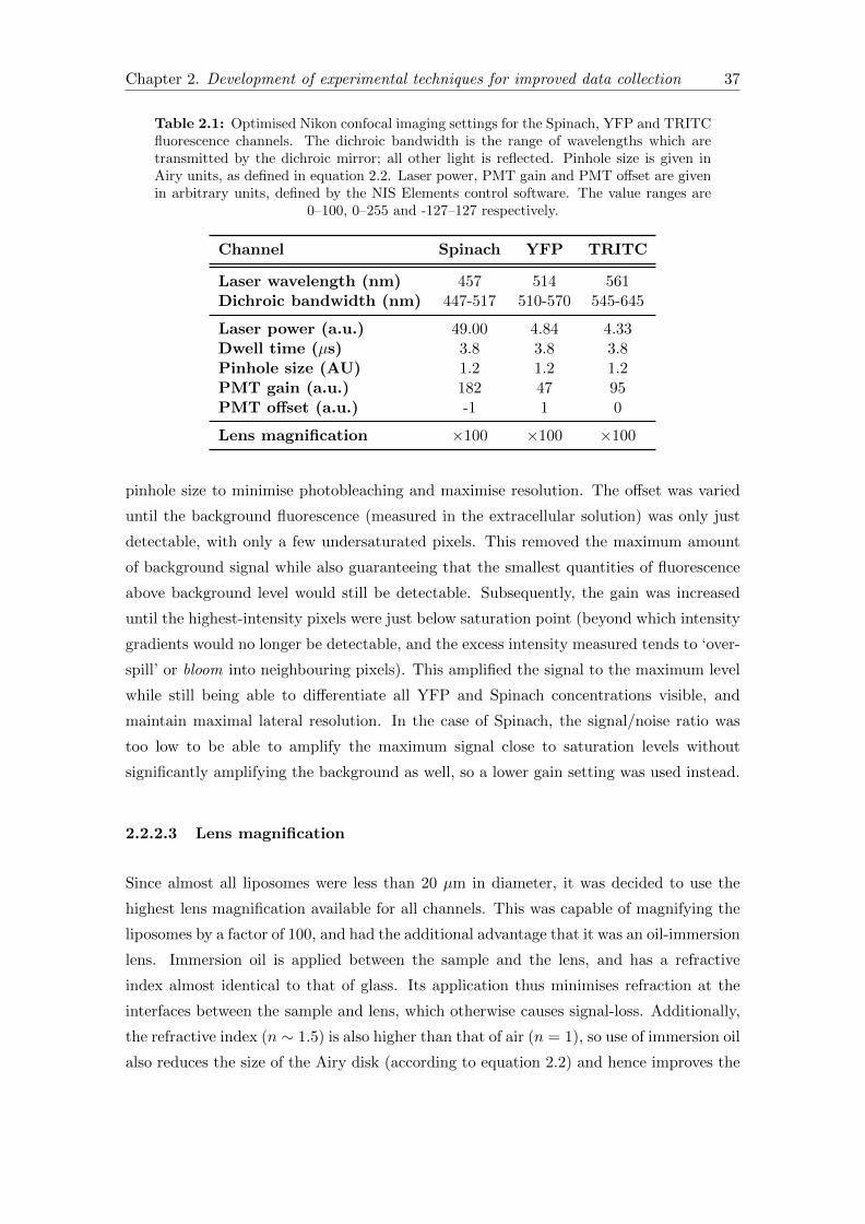
Chapter 2. Development of experimental techniques for improved data collection 37
Table 2.1: Optimised Nikon confocal imaging settings for the Spinach, YFP and TRITCfluorescence channels. The dichroic bandwidth is the range of wavelengths which aretransmitted by the dichroic mirror; all other light is reflected. Pinhole size is given inAiry units, as defined in equation 2.2. Laser power, PMT gain and PMT offset are givenin arbitrary units, defined by the NIS Elements control software. The value ranges are
0–100, 0–255 and -127–127 respectively.
Channel Spinach YFP TRITC
Laser wavelength (nm) 457 514 561Dichroic bandwidth (nm) 447-517 510-570 545-645
Laser power (a.u.) 49.00 4.84 4.33Dwell time (µs) 3.8 3.8 3.8Pinhole size (AU) 1.2 1.2 1.2PMT gain (a.u.) 182 47 95PMT offset (a.u.) -1 1 0
Lens magnification ×100 ×100 ×100
pinhole size to minimise photobleaching and maximise resolution. The offset was varied
until the background fluorescence (measured in the extracellular solution) was only just
detectable, with only a few undersaturated pixels. This removed the maximum amount
of background signal while also guaranteeing that the smallest quantities of fluorescence
above background level would still be detectable. Subsequently, the gain was increased
until the highest-intensity pixels were just below saturation point (beyond which intensity
gradients would no longer be detectable, and the excess intensity measured tends to ‘over-
spill’ or bloom into neighbouring pixels). This amplified the signal to the maximum level
while still being able to differentiate all YFP and Spinach concentrations visible, and
maintain maximal lateral resolution. In the case of Spinach, the signal/noise ratio was
too low to be able to amplify the maximum signal close to saturation levels without
significantly amplifying the background as well, so a lower gain setting was used instead.
2.2.2.3 Lens magnification
Since almost all liposomes were less than 20 µm in diameter, it was decided to use the
highest lens magnification available for all channels. This was capable of magnifying the
liposomes by a factor of 100, and had the additional advantage that it was an oil-immersion
lens. Immersion oil is applied between the sample and the lens, and has a refractive
index almost identical to that of glass. Its application thus minimises refraction at the
interfaces between the sample and lens, which otherwise causes signal-loss. Additionally,
the refractive index (n ∼ 1.5) is also higher than that of air (n = 1), so use of immersion oil
also reduces the size of the Airy disk (according to equation 2.2) and hence improves the

Chapter 2. Development of experimental techniques for improved data collection 38
(a) (b)
(c) (d)
Figure 2.14: Liposome images with Spinach expression in the (a) TRITC, (b) Spinachand (c) YFP channels of the Nikon confocal microscope. An overlay of the three channelsis shown in (d). The mEYFP-Spinach DNA construct shown in Figure 1.2 was used, ina bulk concentration of ∼20 nM. No YFP is seen to express inside these liposomes, buta strong signal in the YFP channel from the liposome membrane indicates a high degree
of crosstalk from TRITC. Scale bar: 5 µm.
imaging resolution. These specifications completed the settings determined for imaging
liposomes using the Nikon confocal microscope, summarised in Table 2.1.
2.2.3 Image quality assessment
An example of a liposome image produced using the Nikon confocal microscope with
the above settings is shown in Figure 2.14. Though the quality of the sample is rather
poor (there is no YFP expression and the circularity of the liposomes is relatively low)
the image illustrates the capabilities and limitations of the Nikon confocal (in its current
state) quite well.

Chapter 2. Development of experimental techniques for improved data collection 39
The edges of the liposomes are seen to be sharply defined, which is necessary for accurate
measurements of liposome size. The axial resolution is also good; a negligible TRITC
signal is observed in the centre of most of the liposomes that are in focus, indicating
that the cell membranes lie outside the optical slice of the image. Measurements of the
liposome sizes indicate that the axial resolution is < 1.5 µm. The interior fluorescence
can thus be measured with very limited crosstalk from TRITC due to spatial localisation.
The zoom and resolution are also sufficiently high for liposomes down to 1 µm in diameter
to be well resolved, such that the mean Spinach and YFP intensities in the interior can
be clearly measured. This is approaching the diffraction limit, and so is as high as can
be expected from a confocal microscope. Though the high zoom limits the camera’s field
of view, this is circumvented by the ‘large image’ option in the NIS elements software,
which allows multiple frames to be stitched together in an arbitrary rectangular grid.
There are two main criticisms of the image quality. The first pertains to the Spinach chan-
nel, in which a background fluorescence (measured in the extracellular solution) measures
approximately 5% of the highest Spinach signal. This was found despite best efforts to
alter the offset, gain and laser power to reduce the background. The entire optical slice
therefore has a distinctly ‘spotty’ green appearance, which must be manually subtracted
to achieve a cleaner image.
The second criticism is the pronounced crosstalk of TRITC in the YFP channel; though
no YFP was produced in the sample shown, the liposome membranes show up clearly in
the YFP channel. This is because the TRITC in the membranes are stimulated by the
YFP excitation wavelength to fluoresce significantly in the bandwidth used for collecting
the YFP emission signal (Figure 2.13). This phenomenon will be discussed further in the
next section.
2.2.4 Relative intensities and crosstalk
Using the imaging settings indicated in Table 2.1, the signal produced by each fluorophore
in each channel was measured to quantify the relative signal intensities and the level of
crosstalk present. To this end, three regions of the samples consisting of only lipids,
Spinach or YFP were identified and the fluorescence was measured for each channel. The
mean relative intensity in each case is presented in Table 2.2. The intensities are scaled
relative to the intensity of the YFP region imaged in the YFP channel, for reference.
It is seen that YFP gave the highest signal in its respective channel, followed by TRITC
and then Spinach. This can be explained by the uniformity of the YFP signal in the bulk
sample used to quantify YFP, allowing the mean signal to be greatly amplified without

Chapter 2. Development of experimental techniques for improved data collection 40
Table 2.2: Crosstalk between the Spinach, YFP and TRITC channels on the Nikonconfocal. Intensities are given relative to the highest measured signal (YFP in the YFPchannel) which takes the value 1.0 by definition. Different fluorophores are labelled inthe three columns, while the three imaging channels are given in the three rows of the
matrix.
Fluorophore/Channel
Spinach YFP TRITC
Spinach 0.36 0.07 0.02
YFP 0.02 1.0 0.04
TRITC 0.08 0.84 0.98
causing saturation anywhere in the image. For TRITC, the presence of multilamellar
liposomes (with higher TRITC concentrations) in some regions of the sample meant that
the mean signal could not be amplified as much before some regions of the image started
to saturate. The low signal from Spinach was due to the low signal/noise ratio, which
was minimised by reducing the gain settings as explained in section 2.2.2.2.
Crosstalk was fairly low (<8% of the desired fluorophore signal) in all cases except one;
that of TRITC in the YFP channel, as mentioned in the previous section. This was unde-
sirably high, and would be unacceptable if it were not for the fact that TRITC and YFP
are spatially distinct in expressing liposomes. Thus, the level of crosstalk shown in Table
2.2 fortunately should not affect gene expression measurements for YFP concentration.
Nevertheless, for reduced crosstalk it may be desirable to use an alternative membrane dye
(such as CellVuer Claret far-red dye [33]) and/or use a different dichroic/laser wavelength
that would minimise the influence of the overlap of the two spectra.
2.2.5 Summary and outlook
The results of the preliminary tests using the Nikon confocal indicate that the image
quality should be sufficient for the purposes of imaging PUREfrex gene-expression in
liposomes larger than to 1 µm in diameter. In this range, the resolution is good enough
to clearly distinguish the membrane edges from both the external solution and their
interior contents. The intensities of the different fluorophores used to track mRNA and
YFP production are high enough to be clearly detectable under carefully chosen channel
settings, and the level of crosstalk is low enough to be able to correct for it during image
processing in most cases.
An important caveat in the interpretation of the above data is that it is based on the level
of mRNA and YFP concentrations after 3 hours of expression. Before this timepoint,
the concentrations will be lower and the signal/noise ratio will be substantially higher,
particularly in the first hour of expression. The above results thus do not necessarily

Chapter 2. Development of experimental techniques for improved data collection 41
apply in the earlier phases of expression. A temperature controller has now been installed
on the Nikon microscope which allows the sample to be incubated at 37 ◦C while it is
positioned on the objective, and should thus allow Spinach and YFP to be imaged at
regular (frequent) timepoints throughout the expression period, and it would be highly
informative to see how similar (and how stochastic) compartmentalised gene expression
kinetics are compared to bulk reactions. Further tests thus ought to be performed to see
at what point Spinach and YFP concentrations become detectable, and how to minimise
this lower bound.
The results for YFP in particular should be retested using a sample with intra-liposomal
YFP, in case the (anticipated) crowded cellular environment affects the fluorescence levels,
or if the intracellular concentrations are quite different from the bulk concentration of the
sample used in this study.
To convert units of fluorescence intensity to units of concentration (necessary for quanti-
tative comparisons between liposomal and bulk expression), calibration experiments must
also be run.
The quality of the image could also be improved by minimising crosstalk, by either choos-
ing an alternative membrane dye or purchasing additional hardware that could allow the
excitation wavelength and/or emission bandwidths to be better optimised for TRITC and
YFP. More advanced imaging options – changing gamma, binning, contrast-enhancement
and time-averaging settings – were not explored in this project, but may also enhance the
image quality. Details on these settings can be found in [28].
Finally, an investigation into the feasibility of using the SIM to image liposomes in higher
resolution is yet to be explored. If trials are successful, then the SIM could permit gene
expression kinetics to be monitored in liposomes down to ∼ 500nm in diameter, when
the current limit is ∼ 1 µm. In Chapter 4, it will be shown that the smallest liposomes
are likely to produce the most interesting stochastic gene expression kinetics, and high-
resolution experimental data from the SIM would be invaluable to validate the in silico
findings.

Chapter 3
Development of a deterministic
model
In this chapter, we begin with a presentation of deterministic modelling techniques used in
the literature to study in vitro gene expression. This is followed by a discussion on former
ways in which the Danelon lab has attempted to model gene expression. Finally, the new
model developed during this project is motivated and presented in detail. A sensitivity
analysis and tests of predictive capacity are then used to validate the final model, and
evaluate its reliability.
3.1 Chemical modelling principles
In the most general sense, a single chemical reaction can be expressed in the form:
reactantsrate−−→ products (3.1)
Reactants are the sum of chemical species that are consumed in the reaction, and products
are the sum of the chemical species that are created during the reaction. The reaction
proceeds at a rate that accounts for both the time taken for the reactants to ‘find’ each
other and the time taken for chemical bonds to be formed/broken. For reactions in bulk
solution, the rate is a function of the reactant concentrations. Similarly, the reactants
and products are also expressed in units of concentration. The order of the reaction with
respect to a particular reactant is defined as the exponent to which the concentration of
that reactant is raised in the rate equation. The overall reaction order is then the sum of
the individual reaction orders with respect to each reactant. Note that if the reagents have
42

Chapter 3. Development of a deterministic model 43
low copy numbers, it may be more pertinent to apply stochastic models instead (as we
shall discuss extensively in Chapter 4), in which reactants, products and rate equations
are expressed in terms of the reactant copy numbers rather than concentrations. The
definition of reaction order is then also correspondingly modified.
The Law of Mass Action states that the rate of a chemical reaction is proportional
to the product of the concentrations of each reagent, with each reagent’s concentration
raised to a power equal to their respective coefficient in the chemical equation [34]. Thus
for instance the reaction:
A + 2B→ C
would have the rate:
k · [A] · [B]2
where k is a constant known as the ‘rate constant’, and [A] and [B] represent the con-
centrations of species A and B respectively. In this example, the overall reaction order is
three.
Conceptually, this law is intuitive when considering the probability for reactant molecules
to diffuse and ‘find’ each other in solution – the higher the reactant concentration, the
faster the reaction is likely to occur. A more rigorous derivation based on a simple
microscopic lattice model can be found in [15]. For stochastic models, the Law of Mass
Action also applies. By changing the reagent concentration to reagent copy number in the
formulation of the law, an identical rate (expressed in units of copy number per unit time
instead of concentration per unit time) can be achieved by modifying the rate constant to
k/V (n−1), where V is the volume of the reaction and n is the number of reacting molecules
per reaction [34].
Strictly speaking, however, the law of mass action only applies for elementary reactions
with a single transition state. Reactions with multiple reaction intermediates must be
broken down into single-step reactions before the law can be confidently applied [34].
Along the same lines, the total number of reagents in a mass action equation is technically
limited to two; the probability of more than two molecules colliding (and hence reacting)
simultaneously is vanishingly small. When more than two reactants are stated, the written
reaction is actually an approximation of multiple bimolecular reactions for which the law
of mass action should technically be applied separately.
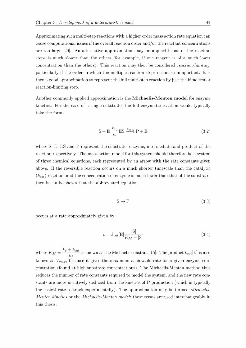
Chapter 3. Development of a deterministic model 44
Approximating such multi-step reactions with a higher order mass action rate equation can
cause computational issues if the overall reaction order and/or the reactant concentrations
are too large [20]. An alternative approximation may be applied if one of the reaction
steps is much slower than the others (for example, if one reagent is of a much lower
concentration than the others). This reaction may then be considered reaction-limiting,
particularly if the order in which the multiple reaction steps occur is unimportant. It is
then a good approximation to represent the full multi-step reaction by just the bimolecular
reaction-limiting step.
Another commonly applied approximation is the Michaelis-Menten model for enzyme
kinetics. For the case of a single substrate, the full enzymatic reaction would typically
take the form:
S + Ekf−⇀↽−kr
ESkcat−−→ P + E (3.2)
where S, E, ES and P represent the substrate, enzyme, intermediate and product of the
reaction respectively. The mass-action model for this system should therefore be a system
of three chemical equations, each represented by an arrow with the rate constants given
above. If the reversible reaction occurs on a much shorter timescale than the catalytic
(kcat) reaction, and the concentration of enzyme is much lower than that of the substrate,
then it can be shown that the abbreviated equation
S→ P (3.3)
occurs at a rate approximately given by:
v = kcat[E][S]
KM + [S](3.4)
where KM =kr + kcat
kfis known as the Michaelis constant [15]. The product kcat[E] is also
known as Vmax, because it gives the maximum achievable rate for a given enzyme con-
centration (found at high substrate concentrations). The Michaelis-Menten method thus
reduces the number of rate constants required to model the system, and the new rate con-
stants are more intuitively deduced from the kinetics of P production (which is typically
the easiest rate to track experimentally). The approximation may be termed Michaelis-
Menten kinetics or the Michaelis-Menten model ; these terms are used interchangeably in
this thesis.

Chapter 3. Development of a deterministic model 45
The above theory will now be applied to the particular case of in vitro gene expression,
first in the context of previous work in literature and followed by applications specific to
the aims of the Danelon Lab.
3.2 Modelling gene expression in bulk solution
For gene expression in bulk solution, deterministic models are used to predict the be-
haviour of the system under different conditions and hence to gain a better understanding
of the processes at work. Michaelis-Menten kinetics are widely used instead of mass-action
equations to model transcription and translation [12, 35]:
DNAv1−→ DNA + mRNA
mRNAv2−→ mRNA + protein
where v1 and v2 are given by:
v1 = kcat,TX · [RNAP] · [DNA]
KM,TX + [DNA]
v2 = kcat,TL · [ribosome] · [mRNA]
KM,TL + [mRNA](3.5)
and subscript TX and TL indicate that the parameters relate to transcription and trans-
lation respectively. The substrates for the two reactions are therefore DNA and mRNA,
and the enzymes are RNAP and ribosome respectively. Note that the substrates are re-
generated on the right hand side of the equation; this signifies the assumption that the
promoter and ribosome binding sites are ‘always free’, which is valid if the (mean) resi-
dence time of RNAP on the promoter is shorter than the timescale of RNAP-promoter
binding. In this way, the full process of mRNA and protein production are encapsulated
by just two chemical equations, with only four rate constants altogether.
The Michaelis-Menten approach is popular for many reasons. Firstly, and most impor-
tantly, the approximations are largely valid. The rate of T7 RNAP binding/unbinding to
its native promoter in E. coli is much faster than the rate of transcription [13, 36], for
example, meaning that the reversible reaction rates are much faster than the catalytic rate
in equation 3.2, as required. The substrate concentrations are not necessarily physically
in excess of the enzyme concentrations, however the approximation that the substrates
are not consumed in the reaction alleviates this condition [15]. Assuming that these ap-
proximations are valid for the particular in vitro gene expression system to be modelled,

Chapter 3. Development of a deterministic model 46
the Michaelis-Menten approach offers an efficient way to reproduce the same mRNA and
protein production kinetics with minimal model complexity.
In particular, minimising the number of parameters (rate constants) to be considered
when fitting experimental data is especially desirable. In general, reducing the number of
degrees of freedom in the fitting algorithm increases the reliability of the fit that is found.
This is due to two main reasons: firstly, with fewer parameter values there are typically
fewer local optima in the parameter space – multiple optima are problematic because they
may offer (near) identical data fits using completely different sets of parameter values.
Secondly, the mRNA and protein production curves are likely to be more sensitive to
variations in each parameter when they are fewer in number; this affects the confidence
with which the parameter fitting is made1.
In addition to transcription and translation, some attempts have also been made to model
the stalling of these processes [12, 37]. The approach taken has varied depending on the
hypothesised cause. Stogbauer et al. (2012) hypothesised that both transcription and
translation stalled due to the depletion of a necessary auxiliary species, on which the
reaction rates are linearly dependent [12]. Production rates v1 and v2 in equation 3.5 are
thus each multiplied by the concentration of a further species (TsR and T lR for tran-
scription and translation respectively). This is equivalent to assuming that the auxiliary
species reacts with the enzyme by (elementary) reversible association/dissociation reac-
tions at a rate that is fast enough for the concentration of the associated complex to
equilibrate on the timescale of the other reactions in the transcription/translation pro-
cesses. TsR is assumed to be depleted at a rate proportional to the transcription rate (so
physically TsR may represent the depletion of NTPs, for example) and TlR is assumed
to be degraded enzymatically (also using a Michaelis-Menten model) by a transcription/
translation independent enzyme. This was because translation consistently stalled after
three hours in their in vitro expression system (PURExpress) – even when DNA was not
added to the mixture until three hours after the other reagents had been prepared (and
hence no transcription nor translation occurred). This model was validated by a successful
fitting to experimental mRNA and protein production kinetics using five different DNA
concentrations ranging over 4 orders of magnitude (from 3.4× 10⁻⁴ to 3.4nM).
Sokolova et al. (2013) attempted to model transcription/translation stalling in more de-
tail by exclusively using mass-action reaction equations [37]. The individual processes
of RNAP-DNA (un)binding, transcription, ribosome-mRNA (un)binding, and translation
were thus all separately modelled. Inspired by Stogbauer, the stalling of expression activ-
ity was also attributed to inactivation of the transcription/translation machinery. In the
1The confidence level for each parameter fit is deduced from the amount by which the parameterneeds to be increased/decreased before the fitting curve deviates from the standard error margins of theexperimental data – see section 3.7.6.

Chapter 3. Development of a deterministic model 47
Sokolova model however, RNAP and ribosomes instead of auxiliary species were identified
as the deactivated reagents, and underwent first order degradation. Sokolova addition-
ally accounted for the consumption of NTPs and amino acids. To this end, RNAP and
ribosomes underwent first order degradation and NTPs and amino acids were ‘blocked’
into single species consumed at a rate proportional to transcription and translation re-
spectively, taking into account the length of the DNA construct. The dependency of
the RNAP/ribosome translocation rate on NTPs and amino acids was accounted for by
treating both processes as bimolecular reactions (between the RNAP-DNA complex and
the NTPs, for example), and modifying the mass-action rate equations accordingly. This
model was validated by fitting experimental mRNA and protein production data from an
E. coli cell lysate -based in vitro gene expression system (5PRIME).
In the literature, it has sometimes also been necessary to model mRNA and/or protein
degradation in order to fit experimental data [12, 35]. This depends on the expression
system being used; protein degradation can be substantial in crude cell lysates – which
contain protein degradation enzymes – but is usually negligible in PUREfrex and PUREx-
press, in which degradation enzymes are absent [6]. Such differences in system composition
partially explain why it was deemed necessary to develop an in-house model of in vitro
gene expression in the Danelon Lab. Difficulties in fitting our experimental data with
established models (such as those of Stogbauer and Sokolova) also highlighted differences
in the system dynamics, which meant that the form of several rate equations also required
modification. These issues will be elaborated upon in the following sections.
3.3 Former lab PUREfrex models
Former attempts to model the PUREfrex system in the lab have taken two different
approaches; the first being Michaelis-Menten based, the other being mass-action based
[13, 20–22]. The advantages of the Michaelis-Menten approach were discussed at some
length in the previous section, and largely explain the motivation behind our usage of
this method [13]. The more complex mass-action approach is most relevant to the work
in this thesis, and has been under active development over recent years. This is due to
our ambition to develop not only a deterministic model for bulk reactions, but a model
that can be straightforwardly adapted for a stochastic simulator to model low-molecule-
number gene expression in liposomes. In order to capture as many sources of stochasticity
as possible, it is desirable to include all elementary reactions of the system in the model
(so that fluctuations in all species amounts and rates can be accounted for), and so
mass-action reaction rates apply. However, in practice this would require an extremely
large and cumbersome model, which can become prohibitively expensive to work with

Chapter 3. Development of a deterministic model 48
computationally [16]. A compromise must therefore be made in order to maintain a
tractable model that still captures the key sources of potential stochasticity; it is most
important to represent species present in low concentrations explicitly, while the effect of
high concentration reagents may be absorbed into rate constants.
To this end, former Master student Alex de Mulder developed an in-house modelling soft-
ware package, Genlink [20]. Genlink automatically computes mass-action reaction rates
from user-input chemical equations, and can perform both deterministic and stochastic
simulations. The deterministic module, coded in C++, can use both genetic and mathe-
matical algorithms to scan the (user-defined) parameter space and thus find the optimal
rate constants to fit (multiple sets of) experimental data. The model can then be vali-
dated with a built-in sensitivity analysis module, to indicate the confidence with which
the rate constants have been fitted. In silico experiments can also be run with the model,
both deterministically and stochastically, to predict what experimental outcomes might
be expected under different initial conditions and/or if additional species are added at a
later time.
Using the Genlink platform, de Mulder created a mass-action model for the PUREfrex
system, which was later simplified by Bachelor student Emma Gerritse [20, 22]. The basic
reaction network – which does not attempt to model transcription or translation stalling
– is as follows (also shown pictorially in Figure 3.1):
Transcription:
DNA + RNAPk1−→ RNAPcomplex + DNA (3.6)
RNAPcomplexk−1−−→ RNAP (3.7)
RNAPcomplexk2−→ RNAP + mRNA (3.8)
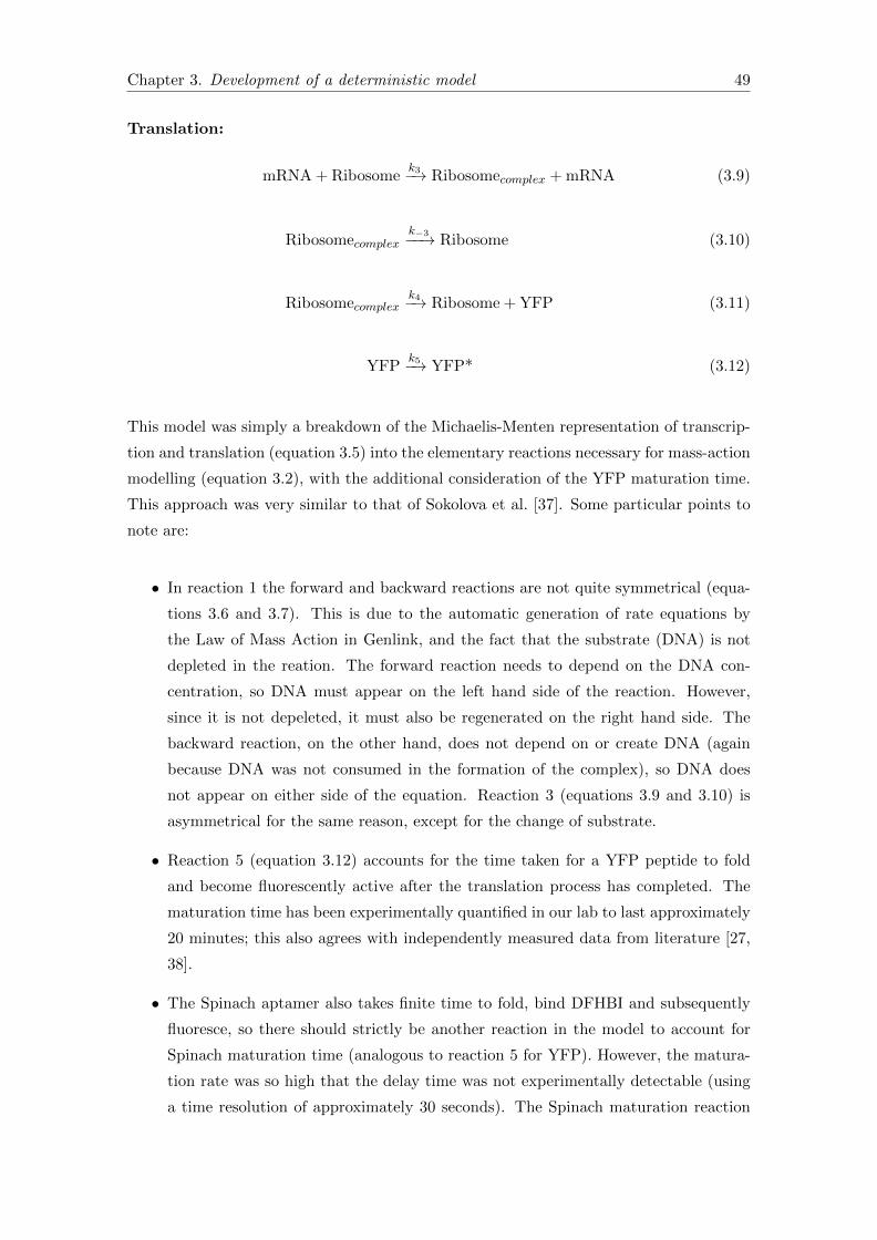
Chapter 3. Development of a deterministic model 49
Translation:
mRNA + Ribosomek3−→ Ribosomecomplex + mRNA (3.9)
Ribosomecomplexk−3−−→ Ribosome (3.10)
Ribosomecomplexk4−→ Ribosome + YFP (3.11)
YFPk5−→ YFP* (3.12)
This model was simply a breakdown of the Michaelis-Menten representation of transcrip-
tion and translation (equation 3.5) into the elementary reactions necessary for mass-action
modelling (equation 3.2), with the additional consideration of the YFP maturation time.
This approach was very similar to that of Sokolova et al. [37]. Some particular points to
note are:
• In reaction 1 the forward and backward reactions are not quite symmetrical (equa-
tions 3.6 and 3.7). This is due to the automatic generation of rate equations by
the Law of Mass Action in Genlink, and the fact that the substrate (DNA) is not
depleted in the reation. The forward reaction needs to depend on the DNA con-
centration, so DNA must appear on the left hand side of the reaction. However,
since it is not depeleted, it must also be regenerated on the right hand side. The
backward reaction, on the other hand, does not depend on or create DNA (again
because DNA was not consumed in the formation of the complex), so DNA does
not appear on either side of the equation. Reaction 3 (equations 3.9 and 3.10) is
asymmetrical for the same reason, except for the change of substrate.
• Reaction 5 (equation 3.12) accounts for the time taken for a YFP peptide to fold
and become fluorescently active after the translation process has completed. The
maturation time has been experimentally quantified in our lab to last approximately
20 minutes; this also agrees with independently measured data from literature [27,
38].
• The Spinach aptamer also takes finite time to fold, bind DFHBI and subsequently
fluoresce, so there should strictly be another reaction in the model to account for
Spinach maturation time (analogous to reaction 5 for YFP). However, the matura-
tion rate was so high that the delay time was not experimentally detectable (using
a time resolution of approximately 30 seconds). The Spinach maturation reaction

Chapter 3. Development of a deterministic model 50
was thus neglected and mRNA is assumed to be fluorescent immediately after tran-
scription has completed.
The above model was validated by a successful fitting to experimental Spinach and YFP
kinetics data from two different DNA concentrations (0.74nM and 7.4 nM), using the
Nelder-Mead and Least Squares optimisation fitting algorithms [22]. Only the first 1.5
hours of kinetics data were used, since after this point the translation rate begins to stall.
1
2
3
4
5
Figure 3.1: Original (‘Genlink’) model reaction network largely devised by De Mulder[20]. RNAP (red oval) binds to the promoter sequence (red) on the template DNA, beforetranscription occurs. This process produces mRNA appended with the Spinach aptamer(bright green). Ribosomes (blue) bind to the RBS (dark green) on mRNA to initiatetranslation. This produces the peptide sequence (orange) which subsequently folds to
produce YFP.

Chapter 3. Development of a deterministic model 51
A more advanced model was therefore necessary to fit the full kinetics curves, and explain
the stalling of transcription and translation.
From literature, the model by Sokolova et al. described in section 3.1 presented the most
complete model of transcription/translation stalling, accounting for both substrate deple-
tion and enzyme deactivation [37]. De Mulder and Just van der Wolf attempted to fit
this model to experimental PUREfrex gene expression data, but found that it was not
possible to obtain a good fit; our data shows that mRNA is produced at a constant rate
for the first few hours of expression (Figure 1.4), while the Sokolova model predicts that
the production rate should decrease noticeably in this period [20, 21]. The discrepancy
is due to the linear dependence of the transcription rates on NTP concentration in the
Sokolova model. Since NTPs are depleted over time, the transcription rate also decrease
monotonically as soon as the reaction starts.
The physical reason why the Sokolova model fails is that by modelling NTP consumption
with a mass-action rate equation, it neglects the fact that NTPs bind reversibly to RNAP
before being incorporated into the growing mRNA [39]. This means that the consumption
would be more accurately modelled using a Michaelis-Menten rate equation, or alterna-
tively by breaking down the consumption step into constitutive elementary steps which
can individually be correctly modelled using mass-action rate equations (akin to reaction
3.2). De Mulder implemented the latter solution successfully in the Genlink model and
found that the influence of NTP depletion alone was sufficient to fit the Spinach pro-
duction data and explain transcription stalling [20]. Experimental evidence from mass
spectrometry also supported this hypothesis (Figure B.1), as did a comparison of the
maximum final mRNA yields with the theoretical maximum computed from the initial
NTP concentrations (Appendix C) [27]. It therefore was not necessary to consider RNA
polymerase inactivation, as Sokolova had suggested [37].
To model the translation plateau, however, amino acid depletion was insufficient to ex-
plain the halt in production. Mass spectrometry data indicated that the amino acid
concentrations did not noticeably reduce by the time translation stalled (Figure B.2); this
was also expected since the initial concentrations of amino acids far exceeded the amount
consumed based on the final yield of YFP. Furthermore, the concentration of tRNAs
in the PUREfrex reaction is also over an order of magnitude lower than that of amino
acids, so it is likely that tRNAs may form more of a bottleneck than amino acids for the
translation rate.
Following the hypotheses of Stogbauer and Sokolova, therefore, de Mulder implemented
ribosome deactivation in the model to account for translation stalling. A constant deacti-
vation rate – as proposed by Stogbauer – was unable to reproduce the observed sharpness
in the transition from linear protein production to the horizontal plateau (Figure B.3).

Chapter 3. Development of a deterministic model 52
Instead, de Mulder hypothesised that the production of a toxic side product during trans-
lation, ’X’, may stimulate ribosome deactivation. Reaction 4 in the model (Figure 3.1)
was thus modified to:
Ribosomecomplexk4−→ Ribosome + YFP + X (3.13)
and ribosome deactivation was modelled by the reaction:
Ribosome + Xk6−→ X (3.14)
This translation-dependent ribosome deactivation model was capable of fitting experi-
mental data, but there was considerable difficulty in finding a consistent deactivation rate
parameter k6 that was capable of fitting multiple datasets (with different DNA concen-
trations) at the same time [20, 22]. This aspect of the model thus was not developed
further at the time.
The Genlink model was shown to be successful at fitting various aspects of experimental
data, and offered some valuable insights in the fundamental behaviour of the PUREfrex
system [20–22]. In particular, it suggested that when the incubation temperature is de-
creased a reduction in the transcription and translation rate (reactions 2 and 4 in Figure
3.1) may extend the expression time, which was experimentally observed [22]. This result
will be discussed further in section 3.7.7.
3.4 New reaction model pre-plateau
Despite its successes, many aspects of the Genlink model still had room for improvement.
Most notably:
1. The initiation, elongation and release factors are not accounted for in the model;
the concentration of ‘Ribosomes’ in the model represents the concentration of the
full range of translation machinery in the model, despite the fact that the actual
concentrations of the individual enzymes vary over more than an order of magnitude.
2. The promoter/ribosome binding site is assumed to be ‘always free’, which is valid
only when the reaction rates satisfy certain conditions (as discussed above). How-
ever, these conditions are not considered when a data fitting is made in Genlink.
Further, during a stochastic simulation these rates can fluctuate substantially. These
effects could potentially render the assumption invalid.

Chapter 3. Development of a deterministic model 53
3. RNAP-DNA and Ribosome-mRNA (un)binding occurs at a fixed rate throughout
the transcription and translation process respectively. This is not true, since bind-
ing/unbinding events primarily occur at the promoter/RBS, and aborted transcripts
rarely occur. The possibility for the RNAP to (un)bind from the DNA strand should
be dependent on a relatively low-concentration ‘pseudo-species’ – promoter-bound
RNAP – which could be subject to substantial fluctuations in a stochastic simula-
tions. This sensitivity to stochasticity would be greatly underestimated using the
original model, since the RNAPcomplex species is far more abundant than promoter-
bound RNAP.
4. Translation cannot start until transcription of the full mRNA molecule is completed.
This is untrue; translation can in fact begin as soon as the ribosome binding site
has been transcribed [2, 40]. Since the ribosome binding site is located close to the
start of the mRNA transcript, the rate of RBS production (and hence translation
initiation) is much faster than that predicted using the original model. Faster rates
are less noisy in stochastic simulations, so stochasticity in translation initiation
would be overestimated when assuming a lower RBS production rate.
5. Translation-dependent ribosome deactivation was a hypothetical cause for the pro-
tein plateau, which was not (yet) supported by experimental evidence.
In this project, the aim was to improve the original model (hereafter referred to as ‘the
Genlink model’) by ameliorating the above weaknesses. Firstly, to remedy points 1-4, the
following model was proposed (schematically represented in Figure 3.2):
Transcription:
Prom + RNAPv1−−⇀↽−−v−1
RNAPb (3.15)
RNAPbv2−→ RNAPc + Prom (3.16)
RNAPcv3−→ RBS + RNAPd (3.17)
RNAPdv4−→ Spinach + RNAP (3.18)

Chapter 3. Development of a deterministic model 54
Translation:
RBS + IF + Ribv5−−⇀↽−−v−5
Ribb (3.19)
Ribbv6−→ Ribc + IF + RBS (3.20)
Ribcv7−→ YFP + Rib (3.21)
YFPv8−→ YFP* (3.22)
where the species names are defined in Table 3.1. Reaction rates are denoted by vn for the
nth reaction, and negative n indicate backward reactions. These are all given by mass-
action rate equations under the standard definition (with rate constant kn), since they
represent elementary reactions in the system. The one exception is (forward) reaction 5,
which is not strictly an elementary reaction (since it has more than two reactants).
Technically, reaction 5 approximates the overall process in which the three initiation
factors IF1, IF2 and IF3 interact with the ribosome and RBS to enable ribosome-RBS
binding. The Law of Mass Action thus does not strictly apply in this case. However, as
mentioned in section 3.1, the rate equation can instead be approximated by the mass-
action rate equation considering only the two species of lowest concentration. This is
because the overall rate would be limited by the rate of the bimolecular reaction between
these two species, assuming that the order in which the multiple reagents interact are not
Table 3.1: Species names used in the new PUREfrex model.
Species Description
Prom Promoter region on DNA constructRNAP T7 RNA polymeraseRNAPb RNAP bound to promoterRNAPc RNAP bound to DNA, transcribing the RBSRNAPd RNAP bound to DNA, transcribing the YFP coding region and Spinach sequenceSpinach mRNA strand with fluorescent Spinach aptamer
RBS Transcribed ribosome binding siteIF Initiation factor IF1Rib RibosomeRibb Ribosome bound to RBSRibc Ribosome bound to mRNA, translating YFPYFP Immature (unfolded, non-fluorescent) yellow fluorescent proteinYFP∗ Folded, fluorescent YFP

Chapter 3. Development of a deterministic model 55
IF
1
2 3
4
5
6
7
8
Figure 3.2: ‘New PUREfrex model’ reaction network, pre-plateau. Key differences withFigure 3.1 include the differentiation between different stages of transcription/translation,the distinction between transcription of RBS and Spinach and the inclusion of the IF(initiation factor) species. Symbols and colour-coding are identical to Figure 3.1 (except
for IF).
important. Applying this approximation, and noting that the concentrations of IF1 and
RBS are (initially) the lowest out of all reactants, the reaction rate v5 is given by:
v5 = k5 · [RBS] · [IF] (3.23)
where [x] represents the concentration of species x in the system.
The most notable difference from the Genlink model is that here the original RNAPcomplex
and Ribosomecomplex species have been divided into subspecies, to represent different
stages of transcription and translation. This improves the model in multiple ways, since
it can:

Chapter 3. Development of a deterministic model 56
1. Restrict dissociation of the complex to occur only at the enzyme binding site (pro-
moter/RBS) or after transcription/translation is completed
2. Produce the RBS before completing transcription of the remainder of the mRNA
transcript (including the Spinach aptamer). This allows translation to begin directly,
which is more faithful to the physical system2.
3. Account for the concentration of initiation factor IF1 instead of ribosome as the
dominant influence for ribosome-RBS binding, as described and explained above.
This replacement could not (accurately) have been applied in the Genlink model,
because IF1 is no longer relevant after the binding step. During translation, the
ribosome concentration should be the only factor limiting the maximum translation
rate.
The improvement in model fidelity unfortunately comes at the cost of an increase in the
number of free (fitting) parameters. As discussed in section 3.1, increasing the number of
fitting parameters typically decreases the confidence level of the final model, and should
thus be minimised as much as possible. However, it has been argued above that the
additional model complexity contributes significantly to improving the accuracy of the
model, and could be particularly valuable for stochastic simulations. In order to minimise
the number of fit optima in the relevant parameter space of the more complex model,
reference data was sought to try to reduce the size of the parameter space.
3.4.1 Estimating parameter values
One clear source of reference data is from experimental studies – focusing on rate quan-
tification – reported in literature. This data is however rather sparse, mainly due to the
difficulty in quantifying rapid reaction rates. Furthermore, the data that does exist cannot
be taken at face value, because differences in experimental conditions (buffer salt concen-
trations and pH, for instance) can substantially affect reaction rates [41]. No detailed rate
quantification has yet been undertaken in the PUREfrex (or PURExpress) system (apart
from the YFP maturation rate k8), so actual rates in our setup may conceivably deviate
by a factor of ten from reported values. With these caveats in mind, literature data for
T7 RNAP binding/unbinding rates were obtained as reference for model parameters k1
and k−1 [36].
The other key source of reference data is from Michaelis-Menten fit results previously
produced in the lab [13], as mentioned in section 3.3. This ‘coarser’ model for transcription
2It is not necessary to consider the possibility for the RNAP to obstruct the passage of the ribosome,because it has been shown experimentally that translation occurs over an order of magnitude slower thantranscription in the PUREfrex system [13].
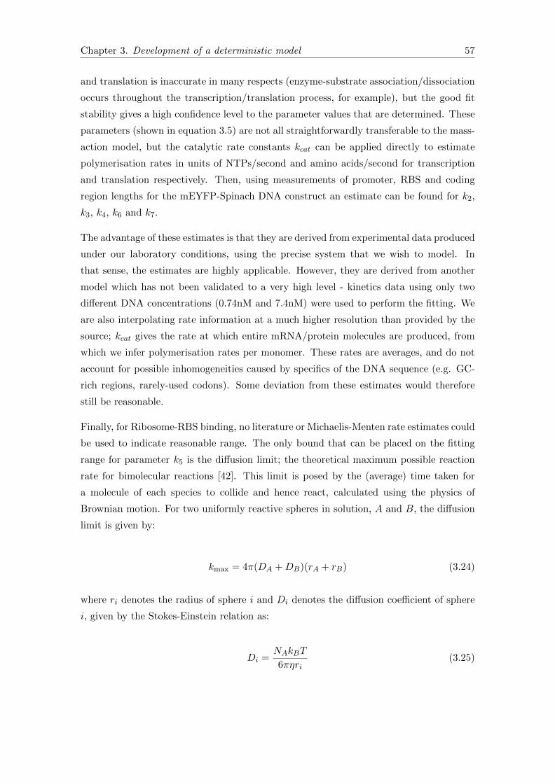
Chapter 3. Development of a deterministic model 57
and translation is inaccurate in many respects (enzyme-substrate association/dissociation
occurs throughout the transcription/translation process, for example), but the good fit
stability gives a high confidence level to the parameter values that are determined. These
parameters (shown in equation 3.5) are not all straightforwardly transferable to the mass-
action model, but the catalytic rate constants kcat can be applied directly to estimate
polymerisation rates in units of NTPs/second and amino acids/second for transcription
and translation respectively. Then, using measurements of promoter, RBS and coding
region lengths for the mEYFP-Spinach DNA construct an estimate can be found for k2,
k3, k4, k6 and k7.
The advantage of these estimates is that they are derived from experimental data produced
under our laboratory conditions, using the precise system that we wish to model. In
that sense, the estimates are highly applicable. However, they are derived from another
model which has not been validated to a very high level - kinetics data using only two
different DNA concentrations (0.74nM and 7.4nM) were used to perform the fitting. We
are also interpolating rate information at a much higher resolution than provided by the
source; kcat gives the rate at which entire mRNA/protein molecules are produced, from
which we infer polymerisation rates per monomer. These rates are averages, and do not
account for possible inhomogeneities caused by specifics of the DNA sequence (e.g. GC-
rich regions, rarely-used codons). Some deviation from these estimates would therefore
still be reasonable.
Finally, for Ribosome-RBS binding, no literature or Michaelis-Menten rate estimates could
be used to indicate reasonable range. The only bound that can be placed on the fitting
range for parameter k5 is the diffusion limit; the theoretical maximum possible reaction
rate for bimolecular reactions [42]. This limit is posed by the (average) time taken for
a molecule of each species to collide and hence react, calculated using the physics of
Brownian motion. For two uniformly reactive spheres in solution, A and B, the diffusion
limit is given by:
kmax = 4π(DA +DB)(rA + rB) (3.24)
where ri denotes the radius of sphere i and Di denotes the diffusion coefficient of sphere
i, given by the Stokes-Einstein relation as:
Di =NAkBT
6πηri(3.25)

Chapter 3. Development of a deterministic model 58
where NA is Avogadro’s constant, kB is Boltzmann constant, T is the incubation temper-
ature of the solution (in Kelvin) and η is its viscosity [43]. This formula is also known as
the Smoluchowski limit.
To apply this theory to ribosome binding, we approximate IF1 and the RBS (the two
species that appear in rate equation 3.23) as uniformly reactive spheres; this is fairly
reasonable for IF1, a globular macromolecule, but quite an approximation for the RBS.
The RBS is certainly not spherical, it is a small part of a much longer and elongated
polymer (mRNA), which may also be attached to a DNA molecule if transcription has
not yet finished. The properties of this ‘object’ as a whole decides the diffusivity of the
RBS species, but only the RBS itself is reactive - the full object thus is not uniformly
reactive.
To get a rough idea of the upper bound posed by the Smoluchowski limit, the RBS
was modelled as a sphere with diameter equal to the length of the RBS sequence itself.
The (approximate) diameter of IF1 was found from literature [44]. Using an incubation
temperature of 37 ◦C (310 K) and the viscosity of water, the above formula gives kmax =
10.4nM−1s−1.
After the above techniques had been applied to limit the ranges for parameter fitting, out
of the 10 rate constants that appear in the reaction scheme (equations 3.15-3.22) only
one, k−5, remained completely unbounded. Furthermore, apart from k5, the other rate
constants were determined to lie within fairly narrow ranges. The degree of constraint
on fitting parameters was thus much higher than in previous work with the Genlink
model [20, 22], so the effective number of ‘free’ parameters was actually reduced, despite
increasing the number of rate constants in the new model. At this stage, it was possible to
confidently extend the model to account for transcription and translation stalling, without
fearing that the number of (new) free parameters that would be added would generate
too much freedom in the model to make a meaningful fit to data. We were finally also
ready to address the fifth and final weakness listed at the beginning of this section; the
treatment of the protein plateau.
3.5 Modelling transcription and translation stalling
3.5.1 Modelling the Spinach plateau
Modelling the Spinach plateau was relatively straightforward, since the most likely cause
for transcription stalling had already been established (as described in section 3.3). The

Chapter 3. Development of a deterministic model 59
depletion of CTP was noted as the key cause, so all that had to be done was to incorporate
the effect of CTP concentration in the model.
NTPs were included in the Sokolova model [37] and also treated in the extended Genlink
model, as described in section 3.3. It was then mentioned that it was necessary to model
the binding of NTPs to the growing mRNA strand as an enzymatic reaction (akin to
reaction 3.2) in order to qualitatively match experimental data, which was treated in the
Genlink model but not in the Sokolova model.
Breaking down the enzymatic NTP binding process into elementary reactions may increase
the accuracy with which stochasticity in each step can be treated, but a Michaelis-Menten
approach was chosen instead for the purposes of this model. This is because the kinetics
of NTP-RNAP binding are not well characterised, so increased model complexity for this
process would also introduce more degrees of freedom that will not be well-bounded by
experimental data. Further, if the binding/unbinding step is fairly rapid compared to the
catalytic (polymerisation) step (as assumed in the Michaelis-Menten approximation), the
inaccuracy in computing stochastic effects is minimal (as shown in Appendix A.2).
Another question is how the sequential addition of almost 1000 NTP molecules to the
growing mRNA should be modelled. A previous attempt from the lab by Kasper van Schie
accounted for each sequential addition separately, and hence every stage of polymerisation
introduced a new species to the model [16]. This created a model with thousands of
species, which was ultimately prohibitively memory-intensive to work with in a stochastic
solver.
An alternative is proposed by De Mulder, which was inspired by ideas presented by
Lazzerini-Ospri et al. Calviello et al. and Frazier et al. [20, 45–47]. In their models, the
binding of individual NTPs to the RNAP-DNA complex forms monomolecular mRNA
‘fragments’, then as soon as the number of fragments equals the full mRNA length they
are together converted into an mRNA molecule. This conversion is instantaneous (since
it is not a physical reaction), and therefore not handled by ODE solvers; a separate
functionality for ‘instantaneous’ reactions is available in Genlink to handle such cases.
The above method is advantageous in that only one intermediate species is introduced,
yet every NTP binding step is still individually modelled and hence all sources of kinetic
stochasticity are accounted for. However, it requires the number of mRNA fragments be
checked at every timepoint - this is easily and accurately achievable in a stochastic solver,
but it was not possible to implement in the deterministic solver when further reactions
also depend on the concentration of completed mRNA strands (e.g. translation) [20].
A further alternative suggested by Tuza et al. effectively considers NTPs being simultane-
ously consumed in batches; each batch being the number of NTPs necessary to compose a

Chapter 3. Development of a deterministic model 60
full mRNA strand [48]. To implement this, a single NTP molecule explicitly binds to the
RNAP-DNA complex, and the remainder of the ‘batch’ is consumed in a separate reaction
(at the same rate). This is much simpler than the above methods, but reduces the ac-
curacy with which stochastic effects are accounted for. A separate consumption reaction
would also have meant that in a stochastic simulation the two different NTP consumption
reactions would in general be asynchronous, which is not physically accurate. Tuza did
not encounter these issues because the model was solely deterministic.
For this project a variation of the Tuza model is used, which is also suitable for stochastic
modelling. Instead of using two separate reactions to represent the simultaneous consump-
tion of NTP batches, we consider an artificial species for which each ‘molecule’ represents
the NTP batch necessary to create an mRNA molecule. This artificial species is then re-
quired to bind to the RNAP-DNA complex before mRNA is produced. The concentration
of this artificial species is then equal to the concentration of NTPs divided by the number
of NTPs consumed per mRNA strand.
The disadvantage of this approach is that the additional stochasticity which should be
introduced by having multiple binding reactions is lost. However, if the NTP binding
reactions occur at a much faster rate than the transcription process as a whole then this
stochastic effect is negligible relative to the overall stochasticity of the system. This is
true, since hundreds of such binding reactions must occur in the time that a single mRNA
is transcribed. The advantages of having fewer reactions and species in the model would
therefore outweigh the disadvantages of having reduced stochasticity.
ATP, GTP, UTP and CTP are also present at different initial concentrations and con-
sumed at different rates in the production of mRNA. The question arises as to whether
every NTP variant should be represented as a separate species in the model. For the
mEYFP-Spinach DNA construct used in this project (Figure 1.2), CTP is the limiting
species that is depleted first (and hence causes transcription stalling). It was therefore
decided to include only CTP in the model. This is a convenient simplification, but leads
to the assumption that energy regeneration in the system is sufficient to prevent ATP
and GTP depleting faster than CTP - this assumption is supported by experimental mass
spectroscopy data (see Appendix B.1). It also means that the influence of ATP and GTP
concentrations on translation cannot be accounted for - this will be further discussed in
the next section.
A final subtlety is that since transcription is broken down in three steps in the model
(Figure 3.2) the consumption of NTPs could be incorporated in any (or all) of these
steps. For simplicity, since the bulk of NTP consumption occurs in the final transcription
step (after the RBS has been produced, and the RNAP-DNA complex is in the RNAPc
state), it was decided to consume NTPs only at that step. However, every transcription

Chapter 3. Development of a deterministic model 61
step should be equally dependent on NTP concentration. If, for example, CTP has been
entirely depleted, but reactions 2 and 3 (Figure 3.1) are not CTP dependent, then RBS
will continue to be produced even after the transcription plateau is reached – this would
be unphysical.
Hence, the final model incorporating NTP depletion modifies reactions 2, 3 and 4 (equa-
tions 3.16, 3.17 and 3.18) to:
RNAPbv2−→ RNAPc + Prom (3.26)
RNAPcv3−→ RBS + RNAPd (3.27)
CTP + RNAPdv4−→ Spinach + RNAP (3.28)
where the concentration of CTP in the model is given by the true concentration of CTP
divided by the number of CTP molecules per mRNA construct. Rates v2 to v4 are given
by:
v2 = k2 · [RNAPb] ·[CTP]
KM + [CTP](3.29)
v3 = k3 · [RNAPc] ·[CTP]
KM + [CTP](3.30)
v4 = k4 · [RNAPd] ·[CTP]
KM + [CTP](3.31)
where KM is the Michaelis constant for CTP-RNAP binding. Thus all three transcription
steps depend on the CTP concentration, but CTP is only consumed in the last stage.
Since the transcription rate is constant for the first few hours of gene expression, it
can be assumed that [CTP] >> KM , and so the quotient in the above expressions is
approximately equal to 1. This is also supported by equilibrium dialysis experiments
which suggest a Michaelis constant of 15 µM, two orders of magnitude lower than the
initial NTP concentrations [39]. Thus k2, k3 and k4 can be estimated using kcat from
the Michaelis-Menten model of PUREfrex gene expression, as described in the previous
section. The addition of CTP in the model thus introduces but one new fitting parameter
to the model, KM .

Chapter 3. Development of a deterministic model 62
3.5.2 Modelling the YFP plateau
Determining the limiting species
Unlike the mRNA plateau, modelling the protein plateau required further experimental
results to determine the physical cause of translation stalling. As mentioned in section 3.3,
it has been established that amino acid depletion was not the cause for the protein plateau
(Figure B.2), so it must be assumed that deactivation of one or more translation-related
enzymes must be the cause. Note that mRNA degradation could not be responsible, since
mRNA is still in peak production at the time translation stalls (Figure 1.4).
The possible deactivated species are thus ribosomes, initiation factors, elongation factors,
release factors and tRNAs. To test which of these species are limiting factors, a fresh
sample of each can be added to a PUREfrex reaction solution in which translation has
plateaued. If one of the above species is being degraded3 in solution, then addition of a
fresh sample should restart translation.
Just van der Wolf attempted such an experiment before this thesis work began [21]. In
four identical PUREfrex samples, equal volumes of either (PUREfrex) solutions B, E, R
or MilliQ was added to each sample. Solution B contains tRNAs, Solution E contains all
the initiation, elongation and release factors, Solution R contains ribosomes and MilliQ
acted as a negative control. It was found that only the addition of solution B restarted
translation after the plateau (Figure B.4), hence it was deduced that translation stalling
was most probably due to the degradation of tRNAs over time.
Care should be taken with the above conclusion, however – in addition to tRNAs, Solution
B also contains NTPs and various buffers. However, though ATP and GTP are necessary
for translation, NTP depletion could not be the cause for translation stalling because
transcription still continues for over an hour after the translation plateau. A further test
also showed that the addition of NTPs only to a PUREfrex reaction after the protein
plateau does not restart translation (data not shown).
Addition of fresh buffer could potentially have a number of positive effects that restarted
translation – remedying changes in pH and salt concentrations during the transcription/
translation reactions, for example. In particular, essential magnesium ions can be precip-
itated by pyrophosphate, a side product of transcription and aminoacylation reactions in
the PUREfrex system [49]. Pyrophosphatase is included in Solution E (in large excess) to
hydrolyse and hence deactivate the pyrophosphate, but it is conceivable that the quantity
3In this chapter, the term ‘degradation’ is used to describe chemical inhibition/deactivation of enzy-matic activity as well as physical breakdown of molecular species.

Chapter 3. Development of a deterministic model 63
Figure 3.3: Comparison of the effects of adding solution B, tRNA or buffer to a protein-plateaued PUREfrex solution (data corrected for background, evaporation and dilutioneffects). Three PUREfrex reactions were run in triplo (the same as duplo, except withthree reaction volumes) and after the protein plateau either solution B, tRNA or bufferwas added to each sample (dashed line). The quantity of each supplementary reagentwas chosen such that the final concentration of fresh reagent equalled the concentrationof the reagent in the initial solution. The ‘plateau’ is seen to have a positive slope whensolution B and buffer were added, but this is attributed to inaccuracies in using thepositive control – due to the substantial (50%) dilution that was performed in these
samples – rather than prolonged expression.
of pyrophosphatase is no longer insufficient after 3 hours of magnesium sequestration, or
that pyrophosphatase itself is deactivated over time.
To test whether translation stalling could be attributed solely (or at least primarily) to
tRNA deactivation, a further experiment was therefore conducted. To three identical
PUREfrex samples, quantities of B solution, pure tRNA solution (Roche, sourced from
E. coli) and (magnesium-rich) buffer solution were separately added. The quantities were
chosen so that the added concentrations of fresh reagents matched their initial concen-
trations in the reaction. It was found that pure tRNA solution alone was sufficient to
restart translation to a comparable level4 and for the same duration as adding the full
B solution, and adding the buffer solution did not have any appreciable effect (Figure
3.3). This supported the hypothesis that tRNA deactivation was the key element causing
translation stalling in the PUREfrex system.
Modelling translation with tRNAs
Following the above experimental findings, it was clear that tRNAs needed to be incor-
porated in the model for translation. Thinking ahead to stochastic simulations, it was
4Although the plateau height appears to be considerably higher for the addition of solution B than theaddition of pure tRNA, it should be noted that this difference also existed in the two samples before theadditions were made. Given further the inaccuracies of the measuring instrument (Clariostar), the heightdifference between these samples is considered insubstantial pending further experimental data.

Chapter 3. Development of a deterministic model 64
also important to model the aminoacylation (and de-aminoacylation5) of tRNAs. This is
because the aminoacyl-tRNA synthetases are among the most dilute of all components
in the PUREfrex system, so the stochasticity of their encapsulation are likely to have a
substantial effect on the gene expression kinetics. The amino acids themselves do not
need to be considered explicitly in the model, since their concentrations are so high that
the synthetases may be assumed to be aminoacylated at all times (Appendix C).
There are two possible approaches for incorporating synthetases in the model – either
assume that the number of aminoacylated tRNAs can be expressed as a simple function
of the synthetase concentration and tRNA concentration (equivalent to assuming that
(de-)aminoacylation reactions are sufficiently rapid that a steady-state is reached), or
represent aminoacylation and de-aminoacylation reactions explicitly in the model. The
former option is simpler, but the latter is a more accurate representation of the system.
In the absence of experimental kinetics data the former would be favoured, but the rates
of aminoacylation and de-aminoacylation have been reasonably well quantified in the
literature. Aminoacylation by tyrosyl-tRNA synthetase was quantified using a Michaelis-
Menten model, and as an approximation these data can be assumed to hold for all twenty
synthetases in the system. The de-aminoacylation rate, assuming that spontaneous un-
binding of amino acids from tRNA does not occur, is equal to the translation rate in units
of amino acids per unit time. This rate has been specifically calculated for the PUREfrex
system by the Danelon Lab, as mentioned in section 3.4.
Consequently, it was decided to represent both aminoacylation and de-aminoacylation
explicitly in the model. For aminoacylation, a new reaction to be added to the system6:
Synt + tRNAv10−−→ AA-tRNA + Synt (3.32)
v10 is given by:
v10 = kcat,aa · [Synt] · [tRNA]
KM,aa + [tRNA](3.33)
≈ k10 · [Synt] · [tRNA] (3.34)
where kcat,aa and KM,aa can be estimated from [50] and [Synt] is the concentration of
synthetases. The approximation holds because the initial (maximum) concentration of
tRNA is much less than KM,aa found in literature, and so for simplicity the approxi-
mation was used in the final model. Since the concentrations of each aminoacyl-tRNA
synthetase in the PUREfrex system is known, the lowest concentration was used in this
5Due to amino acid consumption during translation.6Note that the label v9 has been reserved for the tRNA deactivation reaction, to be discussed later.
Chapter 3. Development of a deterministic model 65
expression (to represent the rate-limiting step). Accordingly, the concentration of the
corresponding tRNA should also strictly be used in the formula, but unfortunately the
relative concentrations of each type of tRNA is not specified in the PUREfrex system.
Thus [tRNA] was instead chosen to represent the concentration of the sum of all tRNAs
in the system. This approximation does not affect the accuracy of the fitting, however,
since appropriate scaling of k10 can cancel out scalings in [tRNA].
De-aminoacylation requires the modification of equations 3.20 and 3.21 (reactions 6 and
7 in Figure 3.2). Following the rationale given above for the consumption of NTPs in
transcription, it was decided that amino acid consumption would occur in reaction 7, in
which the most polymerisation occurs, but the rates of both reactions 6 and 7 should
depend equally on the concentration of AA-tRNAs. These equations are thus modified
to7:
Ribbv6−→ Ribc + IF + RBS (3.35)
AA-tRNA + Ribcv7−→ YFP + Rib + tRNA (3.36)
where v6 and v7 are given by:
v6 = k6 · [Ribb] · [AA-tRNA] (3.37)
v7 = k7 · [Ribc] · [AA-tRNA] (3.38)
It has thus been assumed, similar to the Sokolova model, that tRNA-ribosome interac-
tions follow the Law of Mass Action instead of the Michaelis-Menten model (effectively
saying that the unbinding rate of tRNA from the ribosome is negligible compared to
the binding rate) [37]. This allows us to introduce just one new parameter, instead of
two using the Michaelis-Menten model. If this model is capable of fitting experimental
data satisfactorily, higher complexity can be avoided. This reduces computational cost of
running simulations and may improve fit stability as well.
Modelling tRNA deactivation
The next task was to determine what caused tRNA deactivation; tRNAs could be in-
herently unstable and spontaneously degrade over time, or they could be deactivated by
7ATP and GTP are also converted to ADP and GDP during the translation process, and thus theirconcentrations should also strictly appear in the rate equations. However, if we assume that the energy re-generation in the system maintains their concentrations above that of AA-tRNA, the AA-tRNA–Ribosomeinteraction may be assumed as the rate-limiting step.
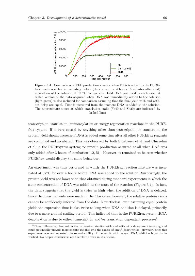
Chapter 3. Development of a deterministic model 66
Figure 3.4: Comparison of YFP production kinetics when DNA is added to the PURE-frex reaction either immediately before (dark green) or 4 hours 15 minutes after (red)incubation of the solution at 37 ◦C commences. 1nM DNA was used in each case. Ascaled version of the data acquired when DNA was immediately added to the solution(light green) is also included for comparison assuming that the final yield with and with-out delay are equal. Time is measured from the moment DNA is added to the solution.The approximate times at which translation stalls (3h40 and 8h20) are indicated by
dashed lines.
transcription, translation, aminoacylation or energy regeneration reactions in the PURE-
frex system. If it were caused by anything other than transcription or translation, the
protein yield should decrease if DNA is added some time after all other PUREfrex reagents
are combined and incubated. This was observed by both Stogbauer et al. and Chizzolini
et al. in the PURExpress system; no protein production occurred at all when DNA was
only added after 3 hours of incubation [12, 51]. However, it remained to be seen whether
PUREfrex would display the same behaviour.
An experiment was thus performed in which the PUREfrex reaction mixture was incu-
bated at 37◦C for over 4 hours before DNA was added to the solution. Surprisingly, the
protein yield was not lower than that obtained during standard experiments in which the
same concentration of DNA was added at the start of the reaction (Figure 3.4). In fact,
the data suggests that the yield is twice as high when the addition of DNA is delayed.
Since the measurements were made in the Clariostar, however, the relative protein yields
cannot be confidently inferred from the data. Nevertheless, even assuming equal protein
yields the expression time is also twice as long when DNA addition is delayed, primarily
due to a more gradual stalling period. This indicated that in the PUREfrex system tRNA
deactivation is due to either transcription and/or translation dependent processes8.
8These differences observed in the expression kinetics with and without a delay are interesting andcould potentially provide more specific insights into the causes of tRNA deactivation. However, since thisexperiment was not repeated the reproducibility of the result with delayed DNA addition is yet to beverified. No deeper conclusions are therefore drawn in this thesis.

Chapter 3. Development of a deterministic model 67
It is difficult to isolate the processes of transcription and translation in order to identify
their separate effects on tRNA deactivation and the protein plateau. In particular, it is
not possible to isolate transcription since translation must always occur for proteins to be
produced. Translation can be isolated from transcription effects by adding presynthesised
mRNA instead of DNA to the PUREfrex reaction mixture, but the instability of presyn-
thesised mRNA (as well as its tendency to form secondary structures in the absence of
translation/RNA binding proteins [40]) leads to a much lower protein yield than in the
case where mRNA is produced in situ.
Nevertheless, such a transcription-independent experiment was attempted to find at least
a qualitative indication of whether translation-related reactions caused (or contributed
to) tRNA deactivation. The resulting YFP production curve is shown in Figure 3.5. It
was found that translation still stalled, despite the absence of transcription in the system.
The expression time (approximately 2 hours) was actually substantially shorter than the
usual 3 hours. A fresh sample of presynthesised mRNA was added after 2.5 hours of
expression, and fresh tRNAs were added after a further 100 minutes.
Since translation did not restart after fresh mRNA was added, it was deduced that the
protein plateau was not due to mRNA degradation or deactivation. Translation did how-
ever restart after tRNAs were added, and continued for more than 1 hour; this ‘restarted’
expression time is comparable to the cases where either B solution or tRNAs are added
to the standard PUREfrex reaction (Figures 3.3 and B.4). This verified that the limiting
Figure 3.5: Translation only in the PUREfrex system. Presynthesised mRNA instead ofDNA is used as a template, and the resulting YFP production curve is shown above (aftercorrecting for background and evaporation effects). Translation stalls after ∼150 minutes,and is not restarted upon addition of fresh mRNA (first dashed line). Fresh tRNAs areadded after a further 100 minutes (second dashed line), at which point translation isrestarted. The fluorescence intensity at the plateau is over ten times lower than whatis typically observed when using DNA instead of presynthesised mRNA as a template
(Figures 2.10 and 2.11).
Chapter 3. Development of a deterministic model 68
factor for the plateau was still tRNA deactivation, the same as when both transcription
and translation processes occurred in the system.
The conclusion from the above experiment was that tRNA deactivation is caused by
translation-related processes in the PUREfrex system, and translation alone is sufficient
to cause tRNA depletion to the point where translation stalls. However, no conclusions
can be drawn regarding transcription-related tRNA deactivation. It is possible that the
presence of transcription would have further accelerated tRNA deactivation. The expres-
sion time was unusually short in the translation-only experiment, but this could have
been due to folding and/or damage in the presynthesised mRNA template, which may
have promoted ribosome pausing during translation. It is possible that this could have
exacerbated tRNA deactivation in some (unknown) way; we thus cannot deduce that the
presence of transcription alleviates tRNA deactivation either.
Given that nothing is known about the influence of transcription on tRNA deactivation,
and that it has been established that translation definitely causes tRNA deactivation,
Occam’s razor was applied in the implementation of translation stalling in the model.
The simplest method (that still accounted for experimental results) was thus chosen.
Transcription was assumed to have no effect on tRNAs, while translation was assumed to
mediate tRNA deactivation by one of the following sets of reactions:
X + tRNAk9−→ X
X + AA-tRNAk9−→ X (3.39)
or alternatively:
X + tRNAk9−→ ∅
X + AA-tRNAk9−→ ∅ (3.40)
where rate equations follow the Law of Mass Action (with rate constant k9) and X is an
artificial species representing the by-product(s) of translation which cause tRNA deacti-
vation. We thus assume that aminoacylation has no effect on tRNA deactivation kinetics.
Equation 3.36 is modified to:
AA-tRNA + Ribcv7−→ YFP + Rib + tRNA + X (3.41)
to model X production. Equations 3.39 imply that X accumulates in the system over
time, and hence the deactivation rate increases steeply over time. Physically, X could

Chapter 3. Development of a deterministic model 69
represent the build-up of a toxin that catalyses the deactivation of tRNAs, or possibly a
by-product that sequesters/precipitates a key ion or other auxiliary chemical necessary
for tRNA to function. Equations 3.40 imply that the side product reacts with tRNA and
hence is also consumed when tRNA is deactivated. Since there was no scientific theory
(to our knowledge) that might favour one model to the other, the final choice between
these two models was made during data fitting, based on mathematical considerations.
It was found that it was only possible to obtain a sharp plateau transition (as seen in
experimental data) using model 3.39, and not 3.40. This can be conceptually explained
as follows. If X is not consumed in the deactivation reaction, its accumulation in the
system is sufficient for the deactivation rate to remain relatively high until tRNAs are
depleted. This allows for a rapid approach to the plateau. If X is consumed, then very
little accumulates in the system and the deactivation rate will begin to slow down much
earlier.
Many other variations to the deactivation mechanism are possible; for instance, X may
need to multimerise or react with other compounds before being able to deactivate tR-
NAs. A Michaelis-Menten rate equation may also be more appropriate if the deactivation
reaction is enzymatic – this was used in the Stogbauer model [12]. A stoichiometry of
1:1 was also assumed in the above model; all of these choices were made for simplicity,
in the absence of any evidence of higher complexity. Difficulties found during data fitting
may however be remedied by modifying the tRNA deactivation reactions by accounting
for one or more of the above effects.

Chapter 3. Development of a deterministic model 70
3.6 Final model presentation
Following the amendments described in section 3.5, the model presented in section 3.4 is
altered to:
Transcription:
Prom + RNAPv1−−⇀↽−−v−1
RNAPb (3.42)
RNAPbv2−→ RNAPc + Prom (3.43)
RNAPcv3−→ RBS + RNAPd (3.44)
CTP + RNAPdv4−→ Spinach + RNAP (3.45)
Translation:
RBS + IF + Ribv5−−⇀↽−−v−5
Ribb (3.46)
Ribbv6−→ Ribc + IF + RBS (3.47)
AA-tRNA + Ribcv7−→ YFP + X + Rib + tRNA (3.48)
YFPv8−→ YFP* (3.49)
tRNA + Xk9−→ X (3.50)
AA-tRNA + Xk9−→ X (3.51)
Synt + tRNAv10−−→ AA-tRNA + Synt (3.52)
Chapter 3. Development of a deterministic model 71
where the reaction rates v1 − v10 are given by:
v1 = k1 · [Prom] · [RNAP] (3.53)
v−1 = k−1 · [RNAPb] (3.54)
v2 = k2 · [RNAPb] ·[CTP]
KM + [CTP](3.55)
v3 = k3 · [RNAPc] ·[CTP]
KM + [CTP](3.56)
v4 = k4 · [RNAPd] ·[CTP]
KM + [CTP](3.57)
v5 = k5 · [RBS] · [IF] (3.58)
v−5 = k−5 · [Ribb] (3.59)
v6 = k6 · [Ribb] · [AA-tRNA] (3.60)
v7 = k7 · [AA-tRNA] · [Ribc] (3.61)
v8 = k8 · [YFP] (3.62)
v9 = k9 · [tRNA] · [X] (3.63)
v10 = k10 · [Synt] · [tRNA] (3.64)
This model will be subsequently referred to as the ’new PUREfrex model’.
There are thus 17 different species and 13 rate constants to be specified in the full model,
introducing 7 new species and 5 new rate constants relative to the Genlink model described
in section 3.3. Together, these additions allow the new model to address the issues raised
at the beginning of section 3.4, with the partial exception of the first point; only the
translation factor with the lowest concentration (IF1) was considered explicitly, the others
were still neglected as before.
This was justified with respect to the initiation factors because we approximate the process
of ribosome binding as a single reaction, absorbing all the initiation factor binding steps
together. Only the limiting bimolecular reaction step (i.e. the one with the lowest reactant
concentrations) thus needs to be considered in the approximated rate, as explained in
section 3.1. The elongation and release factors were not considered in the model because
their concentrations were either similar to or higher than that of ribosomes, and thus
should not have been significant limiting factors in the reactions.
Of course, the model also relies on numerous further assumptions, some of which were
elaborated on earlier. To summarise, the main assumptions are:

Chapter 3. Development of a deterministic model 72
1. No abortive transcription/translation takes place – the RNAP and ribosome can no
longer detach from their templates after translocating off their respective binding
sites;
2. All synthesised Spinach and YFP fluoresce (after maturation);
3. The Spinach aptamer maturation time is negligible relative to the transcription
time;
4. Energy regeneration is sufficient to prevent ATP and GTP concentrations from
decreasing below the CTP concentration or below the tRNA concentration;
5. NTPs and amino acids are only consumed in the last transcription/translation step
(respectively);
6. The effect of translation (including the presence of translation enzymes, substrates
and products) on transcription is neglected;
7. Rates of reactions between more than two reactants can be approximated by the
mass-action equation for the rate-limiting bimolecular interaction;
8. The Michaelis constant for tRNA-ribosome binding is large enough for the unbinding
reaction to be negligible;
9. No chemical species apart from tRNA are degraded or deactivated;
10. All tRNAs are initially active;
11. tRNA degradation is solely due to a single toxic species (‘X’), which is produced at
the same rate as YFP during translation;
12. X catalyses the degradation of tRNA with a 1:1 stoichiometry, but the Michaelis
constant for the interaction is large enough for their unbinding rate to be negligible;
13. X is immediately active once it is produced.
Not all of these assumptions have been experimentally verified. Data from the lab supports
points 3, 4 and 6 [25, 27], but there is no evidence to suggest on what timescale species
X becomes active. Most of the assumptions – including last point – were made just to
simplify the model, in the absence of convincing evidence to the contrary.
A subtle consequence of assumption 7 is that translation kinetics are entirely independent
of the ribosome concentration. The IF1 concentration is substantially lower than the
ribosome concentration, and hence only IF1 appears in the ribosome-RBS binding rate
equation. This would only yield reliable results if the concentration of ‘free’ ribosomes

Chapter 3. Development of a deterministic model 73
(i.e. not bound to mRNA) never drops below the concentration of free IF1 proteins. To
be able to check (and ensure) that this constraint is met in the fitted model, the ribosome
species is represented in the model despite not appearing in any rate equations.
It should also be noted that the model as presented above does not restrict the number
of ribosomes per mRNA strand, though there should be a theoretical maximum (given
by the length of the mRNA strand divided by the length of the ribosome). The ribosome
density can however be controlled by balancing the rate of translocation off the RBS with
the rate of translation of YFP. The ribosome density is thus another property that should
be checked after the rate parameters have been fit to the experimental data.
The selection of the parameter values is thus a sensitive issue, not only to match the model
predictions to the experimental data, but also to ensure that the model meets necessary
physical constraints. The details of the parameter-finding process are thus presented in
the next section.
3.7 Data fitting
3.7.1 Choosing a deterministic modelling platform
In order to find the ‘true’ parameter values for the reaction equations in the new gene
expression model, deterministic modelling software was used to fit model results to experi-
mental data. This software can also be called a ‘deterministic simulator’ or a ‘deterministic
solver’ - these terms are used interchangeably in this thesis. Such a program solves a sys-
tem of coupled differential equations to describe the time evolution of the concentration
of each species in the model. The time evolution for species x, for example, is given by:
d[x]
dt=
np∑i=1
fi(x)−nc∑j=1
gj(x) (3.65)
where x represents the set of all species in the model, np is the number of reactions in
which x is produced, nc is the number of reactions in which x is consumed, and fi and gj
are the rate equations for each of the production and consumption reactions respectively.
By choosing an appropriate set of parameters in fi and gj the aim is to match the time
evolution of the experimentally observable species in the model to kinetics data collected
in the laboratory. This choice can be made by computational algorithms or manually, by
varying parameter values and comparing the model fit to data graphically by eye.
Genlink, being the custom-made software designed specifically for the purposes of research
in our lab, was initially the first choice modelling platform for this project. However, as

Chapter 3. Development of a deterministic model 74
the nature of the model developed, it was found that there were various aspects which
Genlink – at least in its current state – would not be capable of handling.
The major limitation of Genlink was the restriction of rate equations to follow the Law of
Mass Action. This meant that Michaelis-Menten approximations (used in rate equations
3.29-3.31) would not be possible in the model, leading to the necessary creation of six
further reactions and three new fitting parameters. This could potentially improve the
accuracy of stochastic simulations but would not be likely to improve the quality of the fit
of the model to the data or otherwise justify the substantial amount of added complexity.
Rate equation 3.23 does not follow the Law of Mass action either, since three reactants are
present but only the limiting bimolecular reaction is considered for calculating the reaction
rate. In Genlink it would be necessary to neglect either the ribosome or initiation factor
entirely from the model, or use a trimolecular reaction rate, which would not be physical.
The other major drawback of the Genlink interface is that it is strongly focused on
algorithm-based data fitting, with very limited support for manual data fitting. Algorithm-
based fitting techniques are generally superior to manual fitting in terms of both efficiency
and accuracy, requiring little user intervention. It is also easier to quantitatively anal-
yse the fit quality and confidently state when an optimal solution is found. However, if
the experimental data is of variable quality, it is very difficult (and time-consuming) to
bias an algorithm to prioritise fitting more reliable data over other (less reliable, but still
relevant) datapoints. If the algorithm treats all datapoints with equal importance, then
it may either fail to reach a solution, reach multiple solutions, or find a mathematically
optimal solution that does not graphically appear to match the data at all.
As described in Chapter 2.1.6, the experimental kinetics data obtained for the purposes
of this project showed high variability of up to 60%, due to technical difficulties with
the Clariostar plate reader (Figure 2.11). The amount of variability also differed greatly
for experiments run at different DNA concentrations. Certain datasets were thus more
reliable than others, and an algorithm-based data fitting method would be likely to run
into one of the issues mentioned above. A manual fitting method, in which the user can
use their own judgement at every stage of the process, could be much more efficient (and
potentially more accurate) in this case.
Based on the above reasoning, the commercial software Wolfram Mathematicar was cho-
sen as an alternative deterministic modelling and data-fitting platform to Genlink for this
project. Rate equations are unrestricted to any particular form, and manual fitting can be
done quickly and efficiently via the Manipulate interface (Figure 3.6). This customisable
graphic allows all parameters to be varied straightforwardly via sliders or numerical input,
over a range and accuracy limited only by machine precision. The effects of parameter

Chapter 3. Development of a deterministic model 75
Figure 3.6: Simple example of the Manipulate environment interface in Mathematica.Parameters in an expression or system of (differential) equations can be declared asvariables in this environment, so that they can be varied either by numerical input or byusing sliders. An accompanying plot can be specified, which updates in real time as the
parameters are varied.
variation are (almost) instantly visualised in the accompanying plot, which can display
the simulated kinetics curves over the experimental datasets. Manual data fitting then
involves visually comparing the model to the data and adjusting the free parameters until
data at all DNA concentrations are fit well relative to their standard deviations.
The potential downside of manual fitting is that the parameter spaces under investigation
may be extremely large and multidimensional, and without further data to narrow down
the regions of interest a comprehensive exploration of the parameter space could be ex-
tremely time-consuming. The estimates obtained for each parameter in the model were
therefore crucial for fitting success.
3.7.2 Processing experimental data
Even when a manual fitting method is used, a variability of 50% in an experimental dataset
still renders it practically useless for fitting purposes – a wide range of parameters would
be capable of fitting the data to within the range of the standard deviations. Further, the
mean of each set of repeats is not necessarily the ‘truest’ or most reliable representative
dataset to use for fitting, since some repeats were from duplo reactions, while others were
from independent experiments run on different days. The distribution of results from each
repeat was thus often skewed.

Chapter 3. Development of a deterministic model 76
Such high variability was apparent in datasets obtained in the Clariostar, but it is inter-
esting to note that most variability is simply a difference in vertical scaling and not in
the qualitative form of the curves (Figure 2.11). In Chapter 2.1.6, this was attributed to
inaccurate fluorescence measurement rather than variability in gene expression.
As a consequence, if a vertical scaling is applied to the raw datasets from the Clariostar,
the variability in the data due to inaccuracy of the measuring instrument may be sub-
stantially reduced. This process is delicate, however, as it must follow sound rationale to
avoid artificially over-reducing the variability in the data. Since ‘scaling errors’ of the kind
noted in the Clariostar were not present in data from the Eclipse, no raw data obtained
from the Eclipse were processed in this manner.
An important tool that was used for scaling Spinach kinetics data was the theoretical
maximum Spinach yield. As described in section 3.5.1, this could be calculated from the
initial concentration of CTP in the reaction. Instead of using the calibration made in
section 2.1.5, fluorescence units could thus be converted to Spinach concentration based
on the requirement that the peak Spinach concentration was equal to the theoretical
maximum yield (limited by CTP concentration). If it is then assumed that fractional
error in fluorescence measurements are the same for all wavelengths, the corresponding
YFP data can be scaled by the same proportion. This approximation would be justified
if the variability is largely due to formation of differing amounts of condensation on the
well lids in the Clariostar, which would scatter light of all wavelengths by roughly the
same amount. To convert the YFP fluorescence data to concentration units, however, the
calibration from section 2.1.5 must be applied.
The above method can work for reactions with a high DNA concentration, where the
mRNA plateau is sharply approached and the peak is thus well defined. However, for
low DNA concentrations (. 1 nM) the Spinach production rate slows down gradually
over time, and reproducible data from Eclipse measurements indicate that the maximum
CTP-limited yield is not reached. For the datasets obtained using 0.2, 0.74 and 1.0 nM
DNA this reference concentration therefore could not be used for scaling.
Fortunately, the dataset obtained using 0.74 nM DNA was measured in the Eclipse, and
already had relatively low variability (< 10%). Since the dataset obtained using 1.0 nM
DNA in the Clariostar exhibited far more variability (> 30%), an (under)estimate for a
reduced-variability curve was made by scaling the 1.0 nM DNA data such that at the
final timepoint of the 0.74 nM DNA dataset the two Spinach concentrations would be
equal. This was motivated by the proximity of the two concentrations, and the fact that
the underestimation of 1.0 nM DNA dataset could be accounted for in the manual fitting
procedure.
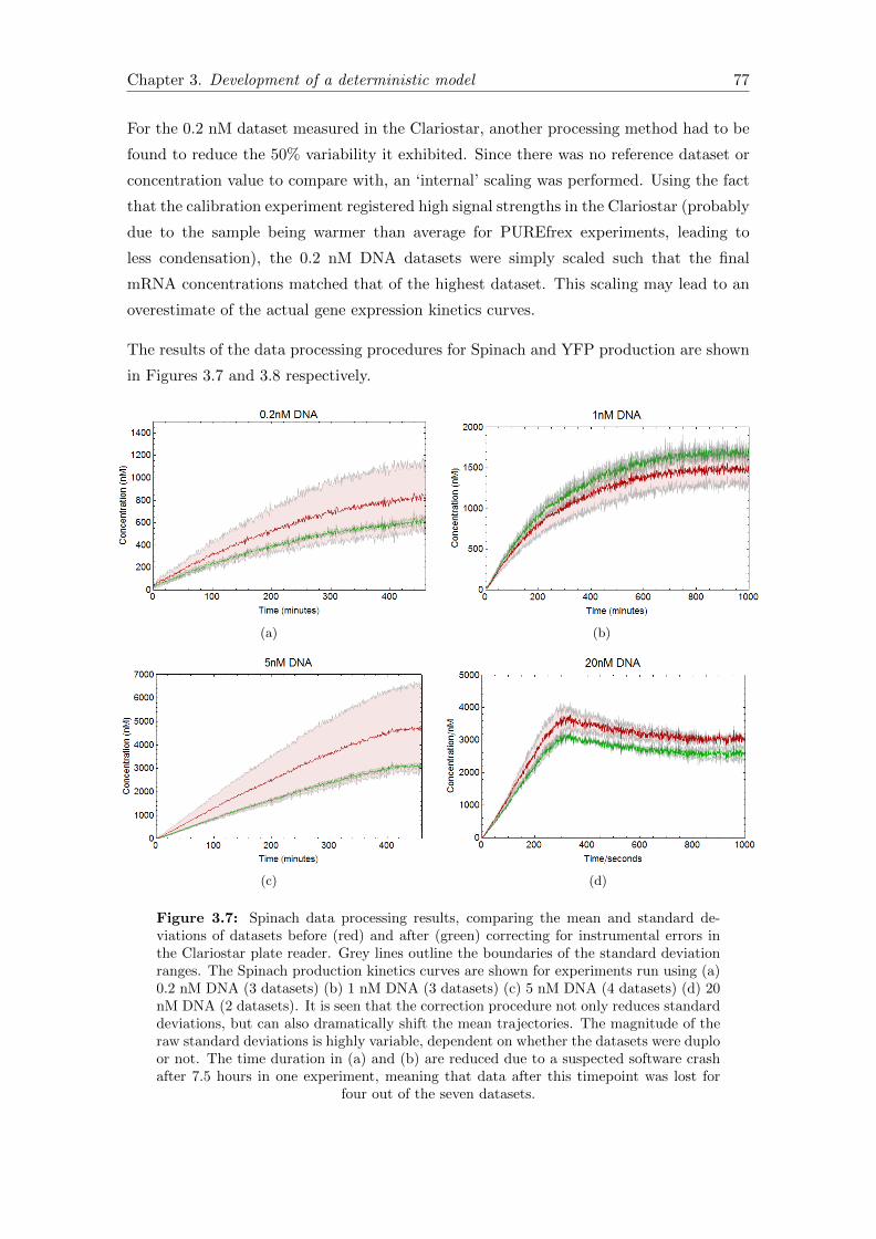
Chapter 3. Development of a deterministic model 77
For the 0.2 nM dataset measured in the Clariostar, another processing method had to be
found to reduce the 50% variability it exhibited. Since there was no reference dataset or
concentration value to compare with, an ‘internal’ scaling was performed. Using the fact
that the calibration experiment registered high signal strengths in the Clariostar (probably
due to the sample being warmer than average for PUREfrex experiments, leading to
less condensation), the 0.2 nM DNA datasets were simply scaled such that the final
mRNA concentrations matched that of the highest dataset. This scaling may lead to an
overestimate of the actual gene expression kinetics curves.
The results of the data processing procedures for Spinach and YFP production are shown
in Figures 3.7 and 3.8 respectively.
(a) (b)
(c) (d)
Figure 3.7: Spinach data processing results, comparing the mean and standard de-viations of datasets before (red) and after (green) correcting for instrumental errors inthe Clariostar plate reader. Grey lines outline the boundaries of the standard deviationranges. The Spinach production kinetics curves are shown for experiments run using (a)0.2 nM DNA (3 datasets) (b) 1 nM DNA (3 datasets) (c) 5 nM DNA (4 datasets) (d) 20nM DNA (2 datasets). It is seen that the correction procedure not only reduces standarddeviations, but can also dramatically shift the mean trajectories. The magnitude of theraw standard deviations is highly variable, dependent on whether the datasets were duploor not. The time duration in (a) and (b) are reduced due to a suspected software crashafter 7.5 hours in one experiment, meaning that data after this timepoint was lost for
four out of the seven datasets.

Chapter 3. Development of a deterministic model 78
(a) (b)
(c) (d)
Figure 3.8: YFP data processing results, comparing the mean and standard deviationsof datasets before (red) and after (green) correcting for instrumental errors in the Clar-iostar plate reader. Grey lines outline the boundaries of the standard deviation ranges.The YFP production kinetics curves are shown for experiments run using (a) 0.2 nMDNA (3 datasets) (b) 1 nM DNA (3 datasets) (c) 5 nM DNA (4 datasets) (d) 20 nMDNA (2 datasets). The raw standard deviations are in general significantly larger thanthose for Spinach (Figure 3.7). The time duration in (a) and (b) are reduced due to asuspected software crash after 7.5 hours in one experiment, meaning that data after this
timepoint was lost for four out of the seven datasets.
It can be seen that the above data processing methods successfully reduced the data
variability to manageable levels and arguably improved the accuracy of the resulting
mean kinetics curves. Variability was reduced to < 5% in all cases except for the YFP
curve using 1nM DNA, where the variability was unchanged. This may indicate that for
these datasets the variability was not due to instrumental errors, but instead perhaps due
to variability in the solution composition or other causes.
For the model-fitting procedure, it was important to bear in mind that the amount of
variability was likely to be underestimated, so some deviation of the fits from the standard
deviation limits could still be reasonable. Further, the mean dataset for 0.2 nM DNA
probably overestimated the Spinach and YFP concentrations, while the mean dataset for
1nM DNA probably underestimated the Spinach and YFP concentrations. These two
Chapter 3. Development of a deterministic model 79
DNA concentrations thus provided the least reliable experimental data, while 0.74 nM
and 7.4 nM DNA data – measured in the Eclipse and therefore not processed – were the
most reliable. Most attention was thus placed on fitting the most reliable data during the
fit procedure.
3.7.3 Fitting protocol
In the initial fitting attempt, all the estimated parameters discussed earlier in the chapter
were employed in the model and a comparison was made to the data. To start with,
only the transcription part of the model was considered in order to fit the Spinach kinet-
ics curve. This was possible because transcription is independent of translation (in the
model). Once a satisfactory fit was made for transcription, the translation part of the
model was fit to YFP data.
Fitting Spinach kinetics data could be done entirely using estimated initial guesses for
all relevant parameter values. This was done in two phases; since KM was much smaller
than the initial CTP concentration, its effect was only felt after approximately 3 hours
of expression. The initial expression period was thus fit with rate constants k1, k−1,
k2, k3 and k4 and the remaining expression was fit using only KM as a free parameter.
These parameter values were then fixed before YFP data was fitted and the remaining
rate constants were tested. One exception was the rate constant for YFP maturation,
which was specifically measured experimentally in the lab and hence also considered a
fixed parameter.
Similarly to mRNA data fitting, the YFP data could also be split into two time periods.
Initially, all tRNAs are assumed to be aminoacylated; in the bulk PURE gene expression
protocol DNA is added last to the reaction solution. For the first minute or so only the
forward aminoacylation reaction thus takes place, which should be more than sufficient
for all tRNAs to be aminoacylated; based on literature data, less than a second is required
using the enzyme concentrations stated in the PUREfrex system [50]. As a consequence,
since the concentration of YFP (and hence also the concentration of side-product X)
is initially low, the first hour or so of YFP production kinetics is almost independent
of the tRNA degradation and aminoacylation rate constants (k9 and k10, in equations
3.39 and 3.34 respectively). Only four parameters k5, k−5, k6 and k7 were thus fitted
against the six datasets for the first hour of YFP production. Parameters k5 and k−5 did
not however have estimated initial starting values; the upper diffusion limit for k5 was
calculated in section 3.4.1 was found to be a gross overestimate when it was attempted in
the fitting. This might have been suspected from the fact that it was also several orders of
magnitude higher than the RNAP-promoter binding rate measured in literature. Hence

Chapter 3. Development of a deterministic model 80
the estimated values of k1 and k−1 were instead used as initial values for k5 and k−5
for the fitting, which assumes that Ribosome-RBS interactions are not too different from
RNAP-promoter interactions.
Once the initial period of YFP production had been satisfactorily fitted, k9 and k10 were
varied to fit the remaining YFP production period, with particular focus on fitting the
final protein yield correctly. Though k10 could be estimated from literature, k9 was com-
pletely unknown since it is a hypothetical reaction which has not yet even been attributed
to specific physical reactants. This was not too problematic in the fitting procedure, how-
ever, because k9 was the key parameter controlling the height of the protein plateau (as
will be demonstrated in section 3.7.6). Further, with six datasets and only two variable
parameters, sufficient experimental data was available to provide a robust fitting.
The fitting procedure was thus split into four distinct phases – fitting early mRNA pro-
duction, fitting late mRNA production, fitting early YFP production, and fitting late
YFP production (in that order). Within each of these phases, the model was checked
against the mean experimental Spinach/YFP data at all DNA concentrations, where the
data had been processed as described in the previous section if necessary. The aim was
to achieve predicted trajectories that lay between the standard deviation error margins
for each dataset. As might be expected, this was never initially the case. The parameter
values were thus adjusted somewhat from their initial estimates, varying the constraints
depending on the reliability of the estimates. Parameters without estimates were given
almost ‘infinite’ leeway (using only the diffusion limit as an upper bound, where appli-
cable), and those with estimates derived from literature were given about an order of
magnitude of leeway. Parameter estimates based on data from the lab were given leeway
based on the experimentalist’s confidence in the accuracy of the specific data. Parameters
with the largest leeway were thus varied first, and those with the smallest leeway were
adjusted last, if at all.
Initial conditions
The initial species concentrations assumed for the model were derived from the precise
composition of PUREfrex; since this information was confidentially disclosed by the man-
ufacturer, they are not reproduced here. The composition of an earlier version of the
PURE system is provided in Appendix C. Most of the initial conditions were straightfor-
wardly transferred from the PUREfrex datasheet, but some choices were not so obvious.
Namely:
• The initial tRNA concentration was calculated from grams/ml to molar units using
the average molecular mass of all types of tRNA in E. coli, and it was assumed
Chapter 3. Development of a deterministic model 81
that all tRNAs are correctly folded9. However, in the PUREfrex system, tRNAs are
obtained from Roche in lyophilised (freeze-dried) form [6], a state in which they are
largely misfolded. There are procedures to refold tRNA from this state, however an
account of tRNA folding kinetics from Bhaskaran et al. suggests that it would be
difficult to exceed 80% fully-folded tRNA in a treated sample [53]. With no explicit
account of tRNA folding in the PUREfrex preparation protocol, the accuracy of the
assumption that all tRNA are folded is unclear.
• As discussed above, all tRNAs are assumed to be aminoacylated at the start of
the experiments. This assumption was based on published kinetics data for tRNA
aminoacylation rates and the fact that de-aminoacylation does not occur until DNA
is present (and subsequently translation occurs). The validity of this assumption is
therefore quite sound.
3.7.4 Fit results and discussion
Using the initial conditions and fitting protocols just described, the final fit results are
shown below. A comparison of fitted parameters with their initial estimates (where ap-
plicable) is provided in Table 3.2, and plots comparing the model-predicted Spinach and
YFP production kinetics with those from experiments are shown in Figures 3.9 and 3.10.
Spinach fit results
Figure 3.9 shows that a good fit for Spinach production kinetics has been found, with
a high fidelity to the estimated parameter values (Table 3.2). In particular, for the
first three hours most of the model curves match the experimental data to within their
respective error ranges. Remembering that most error ranges (apart from those at 7.4
nM and 0.74 nM DNA concentration) were artificially reduced during data processing, a
deviation of ≈ 20% can also be considered reasonable. As expected, at 0.2 nM and 1 nM
DNA concentration the model respectively undershoots and overshoots the experimental
Spinach production rates, but even then the deviation of the model from experimental
data does not exceed 20%.
Beyond the first five hours, however, the model is seen to deviate significantly from the
Spinach experimental data. The model predicts that the Spinach production plateau
should be perfectly flat and the concentration of the plateau should be independent of
the DNA concentration. However, the experimental data shows a weakening Spinach
9From [tRNA] = 56 A260/ml (Appendix C [7]), using the conversion 16 mg = 1 A260 from Roche andthe average molecular mass of tRNA being 25 kD [52] we obtain an initial tRNA concentration of 130 µM.

Chapter 3. Development of a deterministic model 82
(a)
(b)
Figure 3.9: Fit results for Spinach production with 0.2, 0.74, 1, 5 and 20 nM DNA.Comparisons with mean experimental data are shown for (a) the first 3 hours and (b)the first 8 hours of expression. Means and standard deviations are the same as the
post-processed plots in Figure 3.7.
signal over time after transcription stalls at high DNA concentrations. At lower DNA
concentrations, the Spinach concentration does not appear to reduce over time, but seems
to approach a much lower plateau than that obtained at higher DNA concentrations.
These features suggest that mRNA degradation becomes significant after five hours of
expression, and is particularly pronounced at lower DNA concentrations (due to the much
larger deviation from the model at low DNA concentrations). The model was thus only
suitable for use for modelling gene expression kinetics for a period of up to five hours.
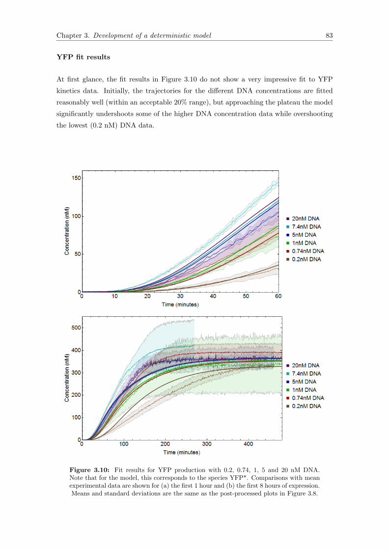
Chapter 3. Development of a deterministic model 83
YFP fit results
At first glance, the fit results in Figure 3.10 do not show a very impressive fit to YFP
kinetics data. Initially, the trajectories for the different DNA concentrations are fitted
reasonably well (within an acceptable 20% range), but approaching the plateau the model
significantly undershoots some of the higher DNA concentration data while overshooting
the lowest (0.2 nM) DNA data.
Figure 3.10: Fit results for YFP production with 0.2, 0.74, 1, 5 and 20 nM DNA.Note that for the model, this corresponds to the species YFP*. Comparisons with meanexperimental data are shown for (a) the first 1 hour and (b) the first 8 hours of expression.Means and standard deviations are the same as the post-processed plots in Figure 3.8.

Chapter 3. Development of a deterministic model 84
Tab
le3.2
:F
itte
dp
aram
eter
valu
es,
dis
tin
guis
hed
into
the
four
gro
up
sin
wh
ich
they
wer
efi
tto
data
(earl
ytr
ansc
rip
tion
,la
tetr
an
scri
pti
on
,ea
rly
tran
slat
ion
,la
tetr
ansl
atio
n).
Lit
erat
ure
sou
rces
for
esti
mate
dva
lues
are
als
ogiv
en.
Note
that
the
fitt
edva
lues
ofk6
an
dk7
wri
tten
bel
oware
giv
enby
the
actu
alfi
tted
valu
esu
sed
inth
em
od
elm
ult
ipli
edby
the
init
ial
con
centr
ati
on
of
tRN
As,
sin
cetR
NA
sw
ere
not
con
sid
ered
inth
eM
ich
ael
isM
ente
nm
od
elu
sed
tod
eriv
eth
ees
tim
ate.
Asi
mil
arap
pro
ach
was
not
nec
essa
ryfo
rth
etr
an
scri
pti
on
rate
con
stants
,d
esp
ite
the
incl
usi
on
of
CT
Pin
the
new
mod
el,
bec
auseK
Mis
larg
een
ou
gh
that
CT
Pdoes
not
aff
ect
the
kin
etic
sin
the
earl
yp
hase
of
exp
ress
ion
.
Para
mete
rD
esc
rip
tion
Un
its
Est
imate
dvalu
eS
ou
rce
Fit
tin
gra
nge
Fit
ted
valu
e
k1
RN
AP
-Pro
mot
erb
ind
ing
nM
−1
s−1
0.03
9[3
6]×
100.
039
k−1
RN
AP
-Pro
mote
ru
nb
ind
ing
s−1
0.48
[36]
×10
1.82
k2
RN
AP
tran
sloca
tion
offp
rom
oter
s−1
0.18
-0.3
3[1
3]×
20.
4k3
Tra
nsc
rip
tion
ofR
BS
regio
non
mR
NA
s−1
0.1
[13]
×2
0.1
k4
Tra
nsc
rip
tion
ofre
mai
nd
erof
mR
NA
s−1
0.00
6[1
3]×
20.
0065
KM
Mic
hael
isco
nst
ant
for
CT
P-R
NA
Pb
ind
ing
nM
15[3
9]×
1053
k5
Rib
osom
e-R
BS
bin
din
gn
M−1
s−1
n/a
–<
10.4
6.96×
10−5
k−5
Rib
oso
me-
RB
Su
nb
ind
ing
s−1
n/a
–n
/a0.
11k6
Rib
oso
me
tran
sloca
tion
offR
BS
s−1
0.06
[13]
×3
0.01
5k7
Tra
nsl
ati
on
of
YF
Ps−
10.
0016
[13]
×3
0.00
16k8
YF
Pfo
ldin
gs−
17.
7×
10−4
[27,
38]
×1
7.7×
10−4
k9
(AA
-)tR
NA
deg
rad
atio
nn
M−1
s−1
n/a
–n
/a6.2×
10−7
k10
Am
inoac
yla
tion
of
tRN
As
nM
−1
s−1
8.4×
10−6
[50]
×10
1.1×
10−5

Chapter 3. Development of a deterministic model 85
However, some features of the experimental data show that, at least with this data sample,
it would be very difficult to improve the fit obtained. Most notably:
• The (initial) production rates of YFP, as well as the total YFP yield, does not in-
crease monotonically with DNA concentration. This is in contrast with the model
predictions, which suggests that the initial YFP production rates and the plateau
height should increase with DNA concentration. However, the data measured in the
Eclipse showed consistently higher expression than the data measured in the Clar-
iostar, and within the measurements taken from each instrument a (small) increase
in yield with increasing DNA concentration is consistently observed. This indicates
that the processing method chosen in section 3.7.2 may have led to a consistent
underestimation of YFP concentration.
• The error ranges are substantially higher than for Spinach data, in both Clariostar
and Eclipse measurements. Furthermore, the final YFP yields at all DNA concen-
trations lie within approximately 20% of each other. Comparing these differences
with the scale of the standard deviations, the difference in the final yields does not
appear to be statistically significant.
The result of the first point is that it was not possible to fit the means of all the datasets
closely. Thus, it was chosen to focus on fitting the lowest and highest DNA concentration
mean data, and as a result of the limited DNA dependence of the curves (mentioned in
the second point) the intermediate data would lie at reasonable values in between.
Neither the lowest (0.2 nM) nor the highest (20 nM) DNA concentrations were measured
with the Eclipse, and hence the closest-fit data were not the ones considered ‘most reliable’
in section 3.7.3. However, the standard deviations for the YFP data measured in the
Eclipse were large enough that even with the alternate focus the model still fitted the
Eclipse data close to or within the error range; albeit at the lower boundary. If instead
focus had been placed on modelling the Eclipse data accurately, then the model would
have substantially mismatched with the Clariostar data.
The model significantly deviates from the data for approximately 2-3 hours when the
system is approaching the plateau. This is partially an artifact of focusing principally on
fitting data at the start and end of expression, as described in section 3.7.3. Using the
reaction model summarised in section 3.6, and the fitting ranges given in Table 3.2, it was
not possible to fit both these regions as well as the intermediate kinetics.
From the shape of the model curves, it appears that the model assumes too high a depen-
dence on (AA-)tRNA depletion. While the experimental curves are approximately linear

Chapter 3. Development of a deterministic model 86
for the first two hours of expression (after an initial delay due to the 20 minute YFP
maturation time), the model trajectories begin to curve much sooner. This suggests that
in the early phase of translation either the degradation rate of tRNAs should saturate (i.e.
be independent of the tRNA concentration), or the effect of tRNAs on translation rate
should saturate. In other words, a Michaelis-Menten model for reaction rates v10 and/or
v6 and v7 should have been used instead of mass-action (where tRNA is treated as the
substrate of the reaction), similar to the treatment of CTP incorporation in transcription.
Due to time constraints, the corrections to the model that this finding entails were not
further investigated. Further, since the experimental YFP data was not of very high
quality, any fitting performed using these reference datasets would not have a very high
confidence. Nevertheless, the fitting that has been found does match the key regions well,
and with a high fidelity to the estimated parameter values.
3.7.5 Validating model assumptions
As mentioned in section 3.6, two assumptions in the model remained to be validated after
the data fitting procedure was completed. Namely:
1. The ribosome concentration exceeds the concentration of IF1 throughout the trans-
lation period;
2. The number of translating ribosomes per mRNA strand does not exceed the theo-
retical limit (posed by the finite ribosome size).
The first assumption was easily checked by plotting the concentration of free ribosomes
[Rib] over time (Figure 3.11). Over 20 hours the free ribosome concentration is seen to
decrease to a minimum of 830 nM, which is over eight times larger than the concentra-
tion of IF1 in the PUREfrex solution. This was found using 20 nM DNA, the highest
concentration used in experiments, to expedite transcription stalling and hence allow the
([RBS]-dependent) free ribosome concentration to reach a steady state as soon as possible.
Since the maximum mRNA yield is independent of the DNA concentration in the model,
the minimum concentration of free ribosomes is also DNA independent. The assump-
tion that IF1-binding remains the rate limiting step in translation initiation for the full
duration of gene expression is thus valid.
The second assumption may be checked by plotting the ribosome density on mRNA over
time. The ribosome density ρ is given by:
ρ =[Ribc] + [Ribb]
[RBS] + [Ribb](3.66)
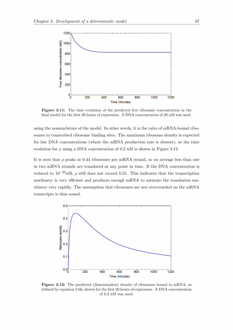
Chapter 3. Development of a deterministic model 87
Figure 3.11: The time evolution of the predicted free ribosome concentration in thefinal model for the first 20 hours of expression. A DNA concentration of 20 nM was used.
using the nomenclature of the model. In other words, it is the ratio of mRNA-bound ribo-
somes to transcribed ribosome binding sites. The maximum ribosome density is expected
for low DNA concentrations (where the mRNA production rate is slowest), so the time
evolution for ρ using a DNA concentration of 0.2 nM is shown in Figure 3.12.
It is seen that ρ peaks at 0.44 ribosomes per mRNA strand, so on average less than one
in two mRNA strands are translated at any point in time. If the DNA concentration is
reduced to 10−20nM, ρ still does not exceed 0.55. This indicates that the transcription
machinery is very efficient and produces enough mRNA to saturate the translation ma-
chinery very rapidly. The assumption that ribosomes are not overcrowded on the mRNA
transcripts is thus sound.
Figure 3.12: The predicted (dimensionless) density of ribosomes bound to mRNA, asdefined by equation 3.66, shown for the first 20 hours of expression. A DNA concentration
of 0.2 nM was used.

Chapter 3. Development of a deterministic model 88
3.7.6 Fit stability and sensitivity analysis
There are two types of checks that can be made to ascertain the level of confidence with
which it may be asserted that the final set of parameters used in the model are close to the
‘true’ values. This is also known as checking the fit stability. Firstly, to check for multiple
fitting optima, different combinations of parameter values (within their respective fitting
ranges) should be used to try to fit the data. If multiple combinations fit the data equally
well, then the fit has a lower confidence level (and vice versa). This is because one cannot
know which of the combinations is the most representative of the physical system.
In order to reduce the occurrences of such optima, further experimental data may be
gathered to narrow the fitting ranges for one or more parameters and/or the model may
be reformulated to reduce ambiguity. One example of such a reformulation is the use of
the Michaelis-Menten approximation to represent reaction 3.2. The fact that three mass-
action rate parameters could be reduced to two with the same fitting capability indicates
that there remains a degree of freedom when all three parameters are used for fitting. In
this case, if kcat � kr then KM ≈ krkf
and it is apparent that only the ratio of kr and kf
is relevant for fitting. There is thus an infinite number of equivalent fitting optima in the
kr and kf dimensions of the parameter space.
The use of Michaelis-Menten in the PUREfrex model presented in this work was partially
motivated by this consideration of fit stability. The elementary mass-action equations
were however maintained for RNAP-Promoter and Ribosome-RBS binding. In the former
case, this was justified by the existence of experimental data to bound the fitting ranges
of k1 and k−1. For the latter, however, no such experimental data could be found. As a
result, the degree of freedom described above was noted in k5 and k−5, leading to a low
fit stability in these parameters.
The other approach for checking fit stability is to perform a sensitivity analysis. In such
a procedure, the sensitivity of the fitted model kinetics to fractional variations in model
parameters are assessed. If there is a low sensitivity to a particular parameter, then the
fit stability is low – large variations in the parameter value do not significantly affect the
fitting curve, so there is no way to tell what the ‘true’ parameter value is within a (broad)
range of possibilities. If the experimental data used to perform the fit is of good quality,
with reliable error margins, the confidence level with which a particular parameter is fit
may be quantified by considering the amount by which it must change before the model
fit exceeds the error margins of the data.
An exhaustive check for multiple fitting optima in the parameter space was not performed
in this project due to the manual fitting procedure; a thorough exploration of the param-
eter space is fairly straightforward when mathematical algorithms are used to perform

Chapter 3. Development of a deterministic model 89
the fitting, simply by seeding with various different initial guesses for each parameter. It
is far more tedious and difficult when performing a manual fitting, however, since each fit
requires extensive work. The only clearly identified multiple optima were in k5 and k−5,
as described above.
The results of a thorough sensitivity analysis are shown in Figures 3.13 and 3.14. The effect
of increasing/decreasing each model parameter by a factor of two is shown for Spinach
and YFP production in the event of low (0.74 nM) and high (20nM) DNA concentration.
In addition to rate constants, the effect of varying initial conditions is also shown to give
insight into the potential sensitivity of the experimental results to pipetting errors.
In general, a much higher sensitivity was shown when using 0.74 nM DNA than 20 nM
DNA. This is not unexpected, since at high DNA concentrations the dependence of the
(a) (b)
(c) (d)
Figure 3.13: Spinach sensitivity analyses for the first 6 h of expression. The effect ofincreasing/decreasing model parameters by a factor of two on the Spinach productioncurve is colour-coded, and split in two groups; rate constants and initial species concen-trations. The unaltered model result is shown in black. Some colours appearing in thelegend do not show in the plots; this is due to overlapping with the unaltered model curveand indicates a low sensitivity to the labelled parameters. Rate constants and speciesconcentrations relating only to translation are not included, since the sensitivity to theseparameters is trivially zero. DNA concentrations of both 0.74 nM ((a) and (c)) as well
as 20 nM ((b) and (d)) are considered.

Chapter 3. Development of a deterministic model 90
production curves are insensitive to changes in DNA concentration. Since both mRNA and
protein production rates are ultimately dependent on DNA concentration, insensitivity to
other rate parameters is not surprising.
For Spinach, the model using 0.74 nM DNA was most sensitive to parameters relating
to transcription initiation. A sensitivity of ∼20% was shown for k1, k−1 and k2 after six
hours of expression. This sensitivity was almost completely lost when using 20nM DNA,
however, for which the transcription rate k4 becomes the most sensitive fit parameter.
This is rational, because when high DNA concentrations are used even low probabilities
for individual RNAP-binding events can allow for enough successful trials to saturate
the transcription machinery. Since the data was fit well by the model at both DNA
concentrations, out of the transcription rate constants only k3 and KM have a low fit
stability.
With regard to initial species concentrations, a high sensitivity to RNAP concentration
was shown for both DNA concentrations. CTP however only affected the Spinach expres-
sion time and final yield, since it is greatly in excess of KM and the stalling of transcription
is directly associated to the depletion (and thus initial concentration) of CTP. Sensitivity
to DNA is high at low DNA concentrations, but low at high DNA concentrations, as
observed during data fitting in section 3.7.4. Pipetting errors in any of these reagents
may therefore cause a high degree of variability in the data, depending on the duration of
the observation time and the DNA concentration used. Particular consideration for the
RNAP concentration is warranted to minimise variation in the initial production rate.
For YFP, the sensitivity to each of the transcription-related model parameters generally
follow the same ranking as Spinach production curves, but the degree of sensitivity is
far lower. The insensitivity to DNA concentration means that there are not significant
differences when either 0.74 nM or 20 nM DNA is used in the sensitivity analysis. The
production curves do not show a sensitivity greater than 5% for any of the transcription
parameters, which is far lower than the variability observed in experiments. This verifies
that it is only necessary to consider fitting to Spinach production data when determining
transcription-related model parameters.

Chapter 3. Development of a deterministic model 91
(a) (b)
(c) (d)
(e) (f)
(g) (h)
Figure 3.14: YFP sensitivity analyses for the first 6 h of expression. The effect ofincreasing/decreasing model parameters by a factor of two on the YFP production curveis colour-coded, and split in four groups; rate constants and initial species concentrationsrelating to transcription, and those related only to translation. The unaltered modelresult is shown in black. Some colours appearing in the legend do not show in the plots;this is due to overlapping with the unaltered model curve and indicates a low sensitivityto the labelled parameters. DNA concentrations of both 0.74 nM ((a), (c), (e) and (g))
as well as 20 nM ((b), (d), (f) and (h)) are considered.

Chapter 3. Development of a deterministic model 92
Interestingly, the YFP curves are also not very sensitive to translation-related rate con-
stants. Apart from k9 and k10, no sensitivity exceeds ∼ 10%. This is due to the regu-
lating effect of tRNA in the system; fast translation rates corresponds to a faster tRNA
de-aminoacylation rate as well as causing faster production of both YFP and X. This
therefore also accelerates tRNA deactivation and a subsequent slowdown of translation.
Conversely, slower translation rates decelerate tRNA de-aminoacylation and deactivation.
Two exceptions to the above are k9 and k10, because they are directly associated with the
behaviour of tRNA in the system. Increasing k9 increases the tRNA degradation rate,
and hence substantially reduces the height of the plateau. Increasing k10 increases the
aminoacylation rate and hence the tRNA can be ‘recycled’ in the translation process more
often before it is deactivated. The translation rate is thus faster during the expression
period and leads to a higher plateau concentration. The trajectories of the sensitivity
curves for these two parameters are so similar that their opposite effects on translation
efficiency almost cancel out. Similarly to Michaelis-Menten kinetics, therefore, only the
ratio of k9 to k10 seems to affect the YFP production kinetics significantly, and the choice
of their precise values are a degree of freedom limited only by the experimental values for
k10 [50]. None of the translation-related rate constants can thus be said to have a high fit
stability.
Unsurprisingly, YFP production kinetics were also insensitive to the concentration of IF1
because it only affects the translation rate, which is normative (as discussed above). The
production curve was however highly sensitive to the initial concentrations of AA-tRNA
and tRNA-synthetase, since they strongly influence the population of active AA-tRNA at
any point in time similarly to k10. Since a much smaller volume of Solution E is pipetted
in the PUREfrex solution than solution B, and also considering that solution E contains
both RNAP and tRNA synthetases, it appears that most caution should be taken when
pipetting solution E. Most care should also be taken to avoid harsh treatment (such as
freeze-thawing) of solution E aliquots, which could degrade the component enzymes.
3.7.7 Predictive capacity
The ultimate validation of a model comes when it successfully predicts behaviour distinct
from the experimental results from which it was derived. For the PUREfrex model, this
meant comparison of model predictions of Spinach and YFP production with experimen-
tal data when parameters other than DNA concentration were varied. There were two
previous experiments by the Danelon lab which could be used for this purpose: one in
which the (initial) concentration of RNAP was varied, and another in which fresh tRNA
was added after the YFP plateau (ibid.).

Chapter 3. Development of a deterministic model 93
Figure 3.15: The effect of adding fresh tRNA after 217 minutes in PUREfrex reactionswith 1 nM DNA. Experimental data is shown in grey, while the model prediction is shown
in red. Experimental data was vertically scaled as described in the main text.
The first experiment was made possible by access to an alternative form of PUREfrex, in
which RNAP is provided in a separate vial instead of being included in Solution E. Zohreh
Nourian obtained experimental data for RNAP concentrations 20%, 50% and 100% of the
standard value, and these results could in principle be directly compared to predictions
from the model. Unfortunately, these data were produced in a single experiment that
has not since been repeated, and the kinetics of the sample using the standard RNAP
concentration were highly anomalous. For instance, protein production continued for over
5 h instead of stalling after 2-3 h as seen in Figure 3.10. As a result, these data were not
deemed suitable for testing the predictive capacity of the model.
As an alternative, data produced during this project (discussed in section 3.5.2) to de-
termine the effect of adding tRNA to a plateaued PUREfrex reaction was used to check
whether the model could reproduce the additional YFP yield and expression time that was
observed. The results of the comparison for 1 nM DNA are shown in Figure 3.15. Both
features were well-predicted by the model, which lends further support to the (largely
hypothetical) form of the tRNA deactivation reactions10.
Unfortunately however, the experimental data was produced in the Clariostar, in which
the calibration of fluorescence intensity to species concentration was inconsistent (as dis-
cussed in Chapter 2). To correct for this, each dataset was vertically scaled so that the
first expression period matched the model prediction. This assumes that the data fitting
performed earlier in this chapter means that the model is ‘correct’ in this time period.
The assumption is reasonable given the thoroughness of the fitting procedure, but strictly
10For ease of implementation, this comparison was made by taking an ensemble average over 100 stochas-tic simulations in the StochPy software package (to be discussed at length in Chapter 4) instead of usingMathematica. This is because StochPy has a built-in capability to handle ‘events’ during the simulation inwhich reagents are added; this is more difficult to program in Mathematica. It will be verified in Chapter4 that the ensemble average corresponds well to the deterministic solution.

Chapter 3. Development of a deterministic model 94
speaking the model can only be said to fit the relative increase in YFP yield upon addition
of tRNA, and not the absolute increase.
3.8 Summary and outlook
The new model for PUREfrex expression has been thoroughly motivated both in terms
of the reaction equations and the final parameter values. The success of the model is
demonstrated by a good match to experimental data during the fitting procedure (using
DNA concentrations ranging over two orders of magnitude).
The new model is an improvement over the previous model used in the lab in several
respects:
• The influence of key low-concentration species (such as tRNA synthetases) on gene
expression are now captured, for the benefit of stochastic simulations;
• The stalling of translation was more accurately represented and rationally justified,
following experimental investigations;
• Data fitting was performed using larger selection of experimental data than before,
with more repeats of each condition and a wider range of DNA concentrations
considered;
• Data fitting of each parameter was guided by experimental data as much as possible,
and accounted for the variability in the reliability of different datasets;
• Assumptions such as low ribosome densities on mRNA were checked and justified;
• Various other assumptions in the original model (listed in section 3.4) were allevi-
ated.
The sensitivity analysis also gave useful indications for the types of data that can best be
used to fit different parameters. For instance, fitting of most transcription parameters are
best performed using Spinach kinetics data at low DNA concentrations, but the fitting of
k4 is best performed using Spinach kinetics data at high DNA concentrations, particularly
using the expression time as a guide. Sensitivity to initial conditions also indicated that
RNAP, tRNA and tRNA synthetase were the most influential enzymes for Spinach and
YFP production curves, and hence that PUREfrex solution E warrants the most caution
for pipetting and storage.
Another step forward is that the new model was able to accurately predict the effect of
adding fresh tRNA to PUREfrex after the protein plateau. Further testing of its predictive

Chapter 3. Development of a deterministic model 95
capacity (with respect to varying RNAP and/or ribosome concentrations, for example)
would give further confidence for the use of the model to predict the effects of varying
any other of its parameters.
The model is however far from perfect. Major drawbacks include:
• The raw experimental data required substantial processing before data fitting, re-
ducing the reliability of the final fit parameters;
• The manual fitting procedure is somewhat subjective;
• Sensitivity analyses revealed that the Spinach and YFP production kinetics are
many rate constants (particularly regarding translation) have a low fit stability;
• A host of assumptions remain in the model, as listed in section 3.6.
The crucial next step for improving the model is the acquisition of more accurate experi-
mental datasets, for determining the model parameters. This would improve the reliability
of the data fitting, particularly because it could pave the way for the use of mathematical
data-fitting algorithms instead of manual fitting procedures. The process is then more
objective and goodness-of-fit statistics can be calculated more straightforwardly. In order
to utilise the algorithm-based data fitting capability of Genlink, it would be also useful
to extend the software so that it can handle reactions with arbitrary rate equations.

Chapter 4
Stochastic modelling
In this chapter, we employ the model established in Chapter 3 to conduct in silico ex-
periments using the stochastic simulation platform StochPy. After introducing the basic
theory behind stochastic modelling, the effects of various sources of stochasticity relevant
to PUREfrex gene expression in liposomes are studied in depth. From the results of these
investigations, an attempt is made to explain the broad distribution of both spinach and
YFP yields found in experiments, as well as the lack of correlation between these two
variables.
4.1 Theoretical Background
The hallmark of stochastic simulators, which sets them apart from deterministic sim-
ulators, is that they account for stochasticity in the rates of chemical reactions. The
way in which this is implemented can vary; stochastic Markov models are based on the
same mathematics used to account for the probabilistic nature of quantum mechanics,
phenomenological models simply add a Gaussian white-noise term to the deterministic
solution, while Monte-Carlo models consider every molecular reaction independently, ran-
domly drawing each rate from the appropriate Poisson distribution (see Appendix A.1)
[54]. All three approaches have been used with success in the past, but while Monte-Carlo
approaches are the most computationally expensive, if all elementary rate constants are
known they also provide the most accurate results [55].
In this thesis, since a detailed model for the system was derived with reasonably high
confidence, a Monte-Carlo approach based on the Gillespie algorithm was employed. The
Gillespie algorithm, and minor variations thereof, are by far the most commonly used
approach for stochastic modelling in modern biological literature [45–47, 56]. It is the
96
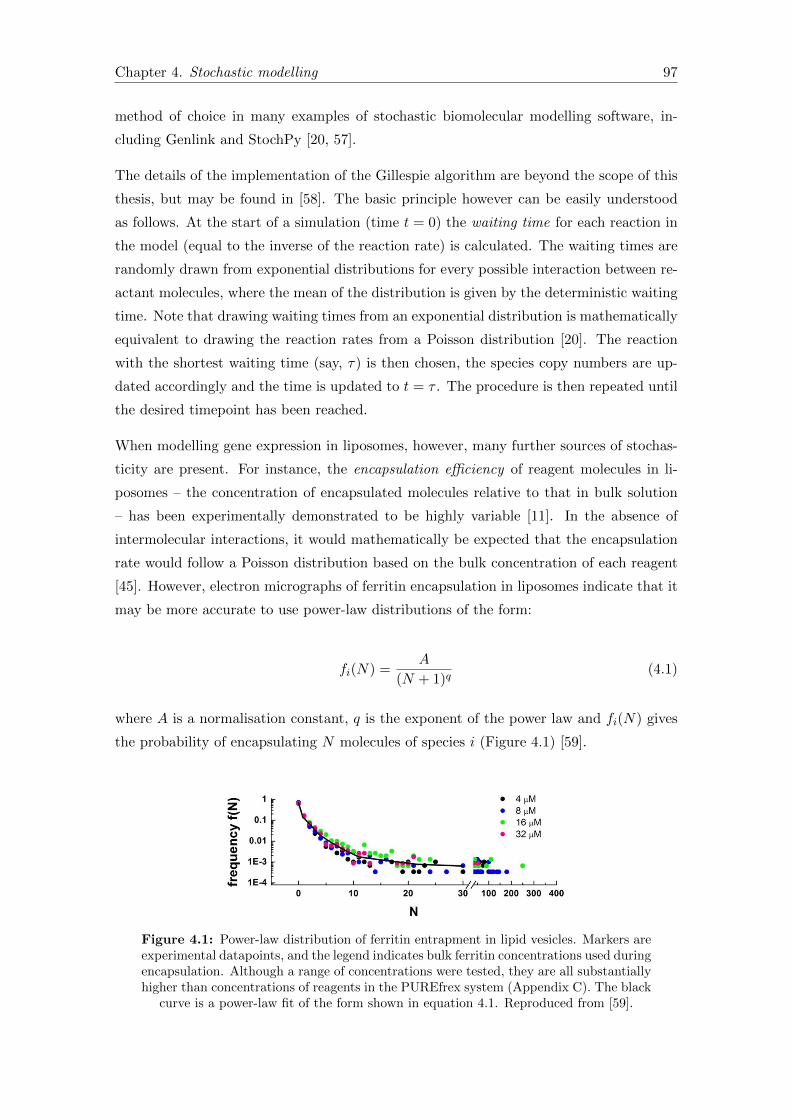
Chapter 4. Stochastic modelling 97
method of choice in many examples of stochastic biomolecular modelling software, in-
cluding Genlink and StochPy [20, 57].
The details of the implementation of the Gillespie algorithm are beyond the scope of this
thesis, but may be found in [58]. The basic principle however can be easily understood
as follows. At the start of a simulation (time t = 0) the waiting time for each reaction in
the model (equal to the inverse of the reaction rate) is calculated. The waiting times are
randomly drawn from exponential distributions for every possible interaction between re-
actant molecules, where the mean of the distribution is given by the deterministic waiting
time. Note that drawing waiting times from an exponential distribution is mathematically
equivalent to drawing the reaction rates from a Poisson distribution [20]. The reaction
with the shortest waiting time (say, τ) is then chosen, the species copy numbers are up-
dated accordingly and the time is updated to t = τ . The procedure is then repeated until
the desired timepoint has been reached.
When modelling gene expression in liposomes, however, many further sources of stochas-
ticity are present. For instance, the encapsulation efficiency of reagent molecules in li-
posomes – the concentration of encapsulated molecules relative to that in bulk solution
– has been experimentally demonstrated to be highly variable [11]. In the absence of
intermolecular interactions, it would mathematically be expected that the encapsulation
rate would follow a Poisson distribution based on the bulk concentration of each reagent
[45]. However, electron micrographs of ferritin encapsulation in liposomes indicate that it
may be more accurate to use power-law distributions of the form:
fi(N) =A
(N + 1)q(4.1)
where A is a normalisation constant, q is the exponent of the power law and fi(N) gives
the probability of encapsulating N molecules of species i (Figure 4.1) [59].
Figure 4.1: Power-law distribution of ferritin entrapment in lipid vesicles. Markers areexperimental datapoints, and the legend indicates bulk ferritin concentrations used duringencapsulation. Although a range of concentrations were tested, they are all substantiallyhigher than concentrations of reagents in the PUREfrex system (Appendix C). The black
curve is a power-law fit of the form shown in equation 4.1. Reproduced from [59].

Chapter 4. Stochastic modelling 98
The liposomes are also not all uniformly sized; their volumes may be distributed over a
fairly broad range depending on their lipid composition [10]. The volume distribution for
DMPC/DMPG liposomes was measured using the Nikon analysis software described in
Chapter 2.2, and was found to range over three orders of magnitude; these results will be
further discussed in section 4.5. In order to model the stochasticity observed in liposomal
PUREfrex gene expression, it was therefore necessary to use modelling software capable of
incorporating the effects of all these sources of variability; it was not sufficient to account
only for stochasticity in reaction rates.
4.2 Software selection
Genlink was initially the first-choice option for executing stochastic simulations, just as
it was for deterministic simulations in Chapter 3. As well as processing stochastic re-
action rates, it contains a built-in module to draw initial species concentrations from a
user-specified Poisson distribution, and is also capable of handling the effects of varying
the liposome volume [20]. A further considerable advantage over most other stochastic
simulators is that it is coded to take advantage of GPU (graphical processing unit) instead
of CPU (central processing unit) computing capability. Use of a GPU allows Genlink to
run thousands of simulations in parallel, while software utilising a CPU can typically run
a maximum of four simulations in parallel. Since stochastic simulations produce different
results every time they are rerun, meaningful data can only be obtained from analysing
the statistical properties of a very large number of simulations (known as an ensemble)
[47]. Running thousands of simulations in parallel, as opposed to sequentially, makes it
feasible to study much larger stochastic models on a much shorter timescale than what
would be possible using a traditional CPU.
Unfortunately, Genlink’s limitation to handling only mass-action rate equations meant
that it could not process the model that was derived in the last chapter. As an alter-
native, the open-source package StochPy was chosen. StochPy, created by the Systems
Bioinformatics group at VU Amsterdam, is a versatile Python-based platform which in-
tegrates smoothly with all the scientific libraries available in Python [57]. Rate equations
can take any form, as can the distribution of initial species concentrations and reaction
volumes. The major disadvantage of StochPy is that it runs on a CPU and cannot run
simulations in parallel – they must all be run sequentially. This limited the maximum
ensemble size (as well as the simulation time and the number of molecules in the system)
that could be produced within a reasonable timeframe. While Alex de Mulder typically
ran 10,000 simulations for any given condition using Genlink, no more than 1000 simula-
tions were attempted in this project using StochPy [20]. Fortunately, for the investigations
Chapter 4. Stochastic modelling 99
that are reported in this chapter, the nature of the results were not much affected when
the ensemble size was increased beyond 100 (data not shown), so the achievable ensemble
size was found to be sufficient for this study.
4.3 Implementing the stochastic model
Several modifications had to be made to the deterministic model derived in Chapter 3
in order to adapt it for use in stochastic simulations. Apart from the change in model
syntax for the different modelling platforms, these included:
• Unit conversion for reaction rate parameters and initial conditions;
• Changes to initial conditions (due to differences in the experimental protocol);
• Consideration of the permeability of the liposome membrane.
These points were relevant to all of the stochastic investigations to be discussed in this
chapter, and will be elaborated in this section. Some other modifications were made
specifically for certain investigations; these will be discussed later in the context of the
relevant studies.
4.3.1 Unit conversions and initial conditions
Due to the change in units from molar concentration to species copy number, the param-
eter values in the deterministic model had to be converted before they could be imple-
mented correctly in a stochastic model. One molecule per cubic micrometre is equivalent
to 1.7 nanomolar units of concentration. Measuring volume in units of cubic micrometres,
therefore, rate constants given with units nM−1s−1 in table 3.2 must be multiplied by 1.7,
while the parameter KM (which has units of nM) must be divided by 1.7 and multiplied
by the liposome volume for the stochastic model.
Similarly, to convert initial species conditions from units of concentration (in nanomolar)
to copy number, the values used in the deterministic model were divided by 1.7 and
multiplied by the volume of the liposome in the simulation. Two exceptions were made
– the initial conditions for aminoacylated and non-aminoacylated tRNA were swapped.
This is because in bulk experiments it was assumed that all tRNAs were aminoacylated
by the time that DNA was added (and the simulation timer was started), as explained
in section 3.7.3. In liposome experiments, however, Solution B (containing tRNAs) is the

Chapter 4. Stochastic modelling 100
last component to be added to the reaction. For stochastic simulations all tRNAs are
therefore assumed to be initially non-aminoacylated.
In deterministic simulations, the DNA concentration was varied to fit different experi-
mental datasets. For all the stochastic simulations to follow, a bulk DNA concentration
(not necessarily equal to the concentration inside liposomes, depending on the encapsu-
lation efficiency) of 20 nM was chosen. This was done for two reasons. Firstly, the DNA
concentration used in recent liposome experiments in the lab – including those described
in Chapter 2.2 and those used to produce Figure 1.6 – ranged between 15 and 30 nM
[13]. The precise value of 20 nM was chosen because the deterministic model was shown
to match the experimental data very well for this concentration, so we can be fairly con-
fident that the model is valid for these expression levels (at least in the deterministic
case).
4.3.2 Modelling membrane diffusion
A further modification may need to be made to the model in order to represent the
passage of small molecules through the liposome membrane. Although it is known that
molecules up to the size of tRNA (and possibly monomeric YFP) are capable of crossing
the membrane, it is not yet known whether this is only possible at the start of the reaction
(when osmotic pressure-induced membrane defects might facilitate their passage) or if
such molecules are able to permeate throughout the expression period [10]. If it is only
possible at the start, then – assuming that the permeation period is short relative to the
expression time – the same reaction model can be used as that presented in Chapter 3.6.
If however small molecules can permeate throughout the expression period, then NTPs,
amino-acids and active tRNAs may never deplete and thus transcription and translation
may never stall. It has been shown that nanoporous fabricated picoliter-volume containers
are capable of sustaining PURE gene expression for several days based on this principle
[60].
Experimental results so far suggest that although gene expression may continue for longer
in liposomes than in bulk reactions, the protein expression rate drops substantially be-
tween 2 and 5 hours (Figure 4.2). This result was consistent across a range of different
lipid compositions and swelling temperatures, and indicates that the liposomes that have
been produced so far in the lab are largely impermeable after the initial period (in which
nutrients must be able to cross the membrane).
The extended expression time compared to bulk reactions may be due to liposomes re-
maining (partially) permeable to tRNAs for the first hour or so, before sealing tight for

Chapter 4. Stochastic modelling 101
Figure 4.2: Experimental liposome kinetics data, indicating average fluorescence levelsand standard deviations measured across the sample of liposomes. Time (in hours) isshown on the x-axis, while fluorescence intensity levels are indicated on the y-axis. Thelegend indicates different lipid compositions used in the liposome membranes. Addi-tionally, ‘cross Tm’ indicates that a temperature cycle was performed in between eachtimepoint to cross the lipid melting point, thereby (temporarily) inducing membrane
defects [61]. Reproduced from [10].
the remainder of the observation period. Alternatively, the membrane may only be per-
meable to smaller molecules, such as NTPs, and impermeable to larger molecules such as
tRNAs. If the toxic side product X is of intermediate size, then a limited but appreciable
degree of outflow may be possible. X would then still accumulate in the liposomes, but
at a reduced rate compared to bulk reactions. This would decrease the rate of tRNA
deactivation and hence explain the extended protein expression time observed in Figure
4.2.
Without further experimental data it was not possible to quantitatively determine the
degree of membrane permeability in liposomes. For the stochastic simulations, therefore,
it was decided to investigate both of the two extrema – either (instantaneous) permeation
only at the start of the reaction, or continuous permeation throughout the expression time.
The two cases will be referred to as ‘impermeable liposomes’ and ‘permeable liposomes’
respectively. In the first scenario the model from Chapter 3 is used without modification,
since each liposome is considered to be an isolated reaction vessel. In the second scenario,
CTP consumption and tRNA deactivation is neglected; the membrane permeability is
assumed to be sufficient to allow CTP concentrations to equilibrate to the external bulk
concentration and to allow X to diffuse out of the liposomes at least as fast as the rate
at which it is produced. Reactions 3.50 and 3.51 are thus removed from the model and
reactions 3.45 and 3.48 are modified to:
RNAPdv4−→ Spinach + RNAP (4.2)
AA-tRNA + Ribcv7−→ YFP + Rib + tRNA (4.3)
respectively, where the rate equations are unchanged from before.

Chapter 4. Stochastic modelling 102
There are three main reasons why the scenario of ‘optimal’ permeability was studied,
despite the evidence that it has not (yet) been achieved in the lab:
1. It may be possible to achieve this level of permeability in future liposomes, using a
different lipid composition and/or different production/treatment methods;
2. The extended protein expression time in liposomes suggests that there may be a
degree of continuous permeability even in our current liposomes;
3. The kinetics of mRNA production in liposomes has not yet been studied. It may
be that current liposomes are fully permeable to NTPs, and transcription does not
plateau at all.
These points suggest that it would be worth investigating liposomes that were continuously
permeable, at least to some degree. For simplicity, it was decided to investigate the
scenario in which all molecules less than or equal to the size of tRNA could diffuse freely,
and X was assumed to fit in this size category1. The maximum beneficial effect of a
permeable membrane could thus be observed, and the effects of intermediate degrees of
permeability could also be qualitatively inferred by interpolating between these results
and the case in which only instantaneous permeability is present.
4.3.3 Validating the stochastic model
Before conducting hypothetical in silico experiments with the stochastic model, it was
necessary to validate that the model could be interpreted correctly by StochPy, and
that unit conversions had been performed successfully. To this end, an ensemble of 100
simulations was executed in StochPy to compare the stochastic Spinach and YFP kinetics
with those found in the deterministic simulation.
Liposomes were assumed to be impermeable, so the system of reactions was identical to
the deterministic case. The initial species concentrations were chosen to equal the bulk
concentrations used in the deterministic model (so all tRNAs were assumed to be initially
aminoacylated), and the liposome volume was fixed to 1 (µm)3 (equivalent to a radius
of 0.62 µm). The only source of stochasticity remaining was thus in the reaction rates.
If the unit conversions had been made correctly, and the model had been transcribed
appropriately, then the mean trajectories of Spinach and YFP production should match
the deterministic solution.
1Initiation factors also fit into this size category, but since they are almost always bound to a (muchlarger) ribosomal subunit, it will be assumed that they are not able to diffuse through liposome membranesin this study.

Chapter 4. Stochastic modelling 103
(a) (b)
Figure 4.3: Validation of the stochastic model. Trajectories of 100 stochastic simula-tions are shown in grey, while their mean and standard deviations are shown in blue.The deterministic curve is shown in red. 20 nM DNA was assumed for all simulations.
The results of the test are shown in Figure 4.3. It is seen that the stochastic and de-
terministic plots match almost perfectly; the small deviations (<2%) can be explained
by the limited ensemble size. As the number of simulations tends to infinity, the mean
trajectories should theoretically approach the deterministic curve exactly. This positive
result confirmed that the stochastic model was valid and suitable for use in the subsequent
investigations.
4.4 Ensemble statistics of interest
The key aim of the stochastic modelling part of the project was to identify the possible
sources of noise that contributed to the broad distribution in YFP and Spinach yields
that was found experimentally (shown in Figure 1.6). To this end, simulations were run
in such a way as to isolate particular sources of noise, and the data was analysed by a
range of methods in order to highlight certain findings. An ensemble of 1000 simulations
was run for each investigation, from which statistical information could be quantified and
visualised to aid in interpreting the data.
The statistical variables and plot types of particular interest are introduced and briefly
defined here. Note that in the context of this work, an ensemble is a set of simulations that
has been run using the same reaction model, rate parameters and probability distributions
for introduced sources of stochasticity. The ensembles in section 4.5.3, for example, have
Poisson-distributed initial species concentrations but fixed cell sizes.
Chapter 4. Stochastic modelling 104
• Ensemble mean, µ. At regular time intervals, the mean Spinach/YFP concentra-
tion is calculated over the ensemble. The rate at which this concentration increases
over time gives the average Spinach/YFP production rate, and the final mean con-
centrations give the average final mRNA/protein yields of the system.
• Ensemble standard deviations, σ. At the same timepoints at which the ensem-
ble means are calculated, the standard deviation of the ensemble’s Spinach/YFP
concentrations are calculated to represent the instantaneous dispersion of the data
about the mean. It is the square root of the variance of the data; the mean square
absolute deviation of each data point from the mean value.
• Fano factor. The Fano factor of a dataset is defined as F = σ2
µ , and is a particularly
useful measure for comparing noise levels in the data to that expected from Poisson
statistics [62]. Unlike the relative standard deviation, σ/µ, F is not biased by
changes in the mean value of Poisson-based distributions. A mathematical property
of the Poisson distribution is that σ2 = µ, so while pure Poisson noise always
has F = 1 the relative standard deviation decreases as the mean increases. If gene
expression was dominated by Poisson noise, the Fano factor of gene expression would
be constant over time while the relative standard deviation would drop. The Fano
factor therefore gives a clearer indication of variations in noise strength caused by
different conditions, being unaffected by any corollary changes in mean values.
• Scatter plots. The distribution of YFP versus Spinach concentrations at a partic-
ular moment in time. This is the simplest way to visualise the spread of protein and
mRNA yields, and check for correlations. The experimental data was presented in
this format in Figure 1.6.
4.5 Identifying independent contributions to stochasticity
4.5.1 Liposome size distribution
The size (distribution) of encapsulating liposomes can affect the level of noise in gene
expression caused by variability in reaction rates and variability in initial conditions.
This is because smaller liposomes tend to enclose a fewer number of reactant molecules,
and vice versa.
Lower species copy numbers tends to enhance the effect of stochasticity in both reaction
rates and encapsulation efficiency. For reaction rates, this is because larger copy numbers
means more reaction events occur per unit time, and so stochasticity in the rate of each
reaction would tend to average out. For encapsulation efficiency, fractional variation in

Chapter 4. Stochastic modelling 105
initial concentrations are enhanced at lower copy numbers because in Poisson distributions
the relative standard deviation is given by σ/µ = 1/√µ (Appendix A.1).
Confocal images of liposomes (such as those shown in Chapter 2.2) reveal highly variable
cell sizes. The distribution of (apparent) cell radii could be measured directly from such
images using the Nikon NIS Elements analysis software. However, the apparent radii from
the images are not in general equal to the true cell radii. The confocal image shows only
a thin optical slice at the imaging plane, which has a vanishingly small probability of
exactly intersecting the centre of every liposome in the field of view. The true cell radii
are thus almost always underestimated using this method of measurement.
Nevertheless, if we assume that the liposomes are perfectly spherical and the image plane
intersects the liposomes at different heights with uniform probability, the average amount
by which a cell radius is underestimated can be calculated. The mathematical derivation
is provided in Appendix A.3, and shows that on average the apparent radius r is equal to√23R, where R is the true cell radius. Dividing the measured radius distribution by
√23
thus gives a better estimation of the liposome size distribution present in the sample.
A histogram showing the corrected cell radius measurements from a sample of 280 DM-
PC/DMPG liposomes is provided in Figure 4.4. A continuous probability distribution
that closely matches this data is the lognormal distribution, which takes the form:
f(x;µ, σ)1
xσ√
2πe−
(lnx−µ)2
2σ2 , x > 0 (4.4)
where f denotes the probability density function for variable x (in this case, the liposome
radius), and µ and σ are the mean and standard deviation of the natural logarithm lnx
respectively [63]. A fit was made to the liposome radius data using a maximum likelihood
algorithm in Wolfram Mathematicar. The resulting curve is shown in Figure 4.4, and
uses parameter values µ = 0.26 and σ = 0.39.
These data indicate that the mean liposome radius is approximately 1.4 µm, and the vast
majority of liposomes have a cell radius of between 0.8-2.0 µm. The absence of liposomes
with radius less than 0.8 µm in the experimental data was due to the limited resolution
of the confocal microscope - it was not possible to clearly observe and measure liposomes
with an apparent diameter smaller than approximately 1.2 µm, which (after applying
the correction factor) translates to a cell radius of 0.8 µm. In the microscope images,
small blurred patches of fluorescence in the TRITC channel indicated there were smaller
liposomes present (though an analysis by super-resolution microscopy would be necessary
to prove this assertion). The shape of the distribution below 0.8 µm is therefore currently

Chapter 4. Stochastic modelling 106
Figure 4.4: Cell radius distribution for DMPC/DMPG liposomes, corrected for varia-tions in viewing plane. Experimental data is shown by the histogram, while the smoothcurve shows the fit made using the lognormal distribution given in equation 4.4 with
parameters µ = 0.26 and σ = 0.39.
unknown, but for the purposes of this study we postulate that it continues to follow the
lognormal distribution determined from the existing data.
4.5.1.1 Selection of fixed reaction volumes
As a result of the volume-dependence of noise due to reaction rates and initial conditions, it
was decided to test three different cell sizes in the subsequent investigations. A preliminary
study was conducted to identify the range of liposome sizes that could be used for this
purpose. It is most interesting to look at very small cells, since they are likely to contain
the noisiest dynamics. However, if the chosen cell size is too small, no expression may be
seen at all. According to Poisson statistics, the probability of encapsulating at least one
molecule of each necessary species for gene expression becomes increasingly improbable
for very small liposomes [59].
An ensemble of simulations using a range of reaction volumes was therefore run to find
how the probability of expression depended on cell size. The fraction of the ensemble
which produced at least one molecule of YFP and/or Spinach was then plotted (Figure
4.5).
It was found that the quantity of liposomes exhibiting Spinach expression became appre-
ciable (> 50%) for radii > 0.3 µm. YFP expression however was only appreciable for cell
radii greater than 0.5 µm. 100% expression rates were found for cell radii greater than
0.8 µm.
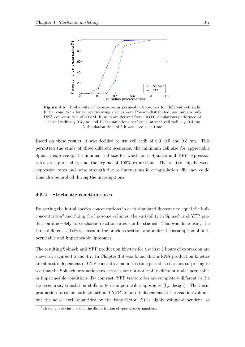
Chapter 4. Stochastic modelling 107
Figure 4.5: Probability of expression in permeable liposomes for different cell radii.Initial conditions for non-permeating species were Poisson-distributed, assuming a bulkDNA concentration of 20 nM. Results are derived from 10,000 simulations performed ateach cell radius 6 0.3 µm, and 1000 simulations performed at each cell radius > 0.4 µm.
A simulation time of 5 h was used each time.
Based on these results, it was decided to use cell radii of 0.3, 0.5 and 0.8 µm. This
permitted the study of three different scenarios; the minimum cell size for appreciable
Spinach expression, the minimal cell size for which both Spinach and YFP expression
rates are appreciable, and the regime of 100% expression. The relationship between
expression rates and noise strength due to fluctuations in encapsulation efficiency could
thus also be probed during the investigations.
4.5.2 Stochastic reaction rates
By setting the initial species concentrations in each simulated liposome to equal the bulk
concentration2 and fixing the liposome volumes, the variability in Spinach and YFP pro-
duction due solely to stochastic reaction rates can be studied. This was done using the
three different cell sizes chosen in the previous section, and under the assumption of both
permeable and impermeable liposomes.
The resulting Spinach and YFP production kinetics for the first 5 hours of expression are
shown in Figures 4.6 and 4.7. In Chapter 3 it was found that mRNA production kinetics
are almost independent of CTP concentration in this time period, so it is not surprising to
see that the Spinach production trajectories are not noticeably different under permeable
or impermeable conditions. By contrast, YFP trajectories are completely different in the
two scenarios; translation stalls only in impermeable liposomes (by design). The mean
production rates for both spinach and YFP are also independent of the reaction volume,
but the noise level (quantified by the Fano factor, F ) is highly volume-dependent, as
2with slight deviations due the discretisation of species copy numbers.

Chapter 4. Stochastic modelling 108
expected. It is seen that F < 1 for a cell radius of 0.8 µm, indicating sub-Poisson noise
levels, while F is an order of magnitude larger for a cell radius (R) of 0.3 µm. This
was also expected, as mentioned in section 4.5.1. Interestingly, for the first five hours
of expression the (time-averaged) magnitude of the Fano factors for YFP and spinach in
the same cell volume are very similar, despite the fact far more reactions occur in the
production of YFP than Spinach.
Apart from Figure 4.6(d), the Fano factors are generally constant in time. This indicates
that stochasticity in reaction rates does not usually vary significantly as the reaction
progresses. For YFP production in impermeable liposomes, the time evolution of the
Fano factors are more complex. Due to the regulatory effect of X production during
translation, mentioned in Chapter 3.7.6, the Fano factor drops steeply from its initial
value during the expression period. Once translation begins to plateau, however, the
Fano factor increases and tends towards a constant value (which is still lower than the
initial value). Conversely, for mRNA the Fano factor in impermeable liposomes tends to
drop during the fifth hour of expression. This is because the depletion of CTP starts to
be felt at this point, and since the initial concentration of CTP is fixed the height of the
mRNA plateau is also fixed. The Fano factor for mRNA thus continues to decrease and
eventually tends to zero as the plateau is approached (not shown).
The relatively small magnitude of the standard deviations (and hence Fano factors) in
the kinetic trajectories indicate that stochasticity in reaction rates alone could not cause
as large a variability in Spinach and YFP yields as that observed in experiments (Figure
1.6). This is further illustrated in the scatter plot shown in Figure 4.8. After three hours,
the spread of Spinach and YFP yields are still very restricted. Though the distributions
do broaden substantially as the cell volume is reduced, the highest and lowest expression
levels never differ by more than a factor of two.
Within these distributions, it may initially seem surprising that the Spinach and YFP
yields are uncorrelated. However, this is simply because the quantity of mRNA produced
after three hours far exceeds that required to saturate the translation machinery (evi-
denced by the ribosome density in Chapter 3.7.5). The variability in YFP production is
thus independent of the (small degree of) variability in Spinach yields. This explanation
cannot explain the lack of correlation seen in Figure 1.6 however, where extremely low
mRNA concentrations can produce YFP concentrations that vary over an order of mag-
nitude. Stochasticity introduced from initial conditions and volume distributions must
thus be necessary to explain the scale of uncorrelated variability observed in experiments.

Chapter 4. Stochastic modelling 109
(a) (b)
(c) (d)
Figure 4.6: Reaction rate noise kinetics in impermeable liposomes, data from an en-semble of 1000 simulations. (a) mRNA time series (b) YFP time series (c) mRNA Fanofactors (d) YFP Fano factors. The legend gives the value of the cell radius, R, used inthe simulations. Note that the first datapoint in Fano factor plots are located at the
origin due to the use of fixed initial conditions in the simulations.
4.5.3 Stochasticity from initial conditions
For the next set of simulations, stochasticity in initial conditions were considered in addi-
tion to noisy reaction rates. As mentioned in section 4.1, there are two alternative theories
to model the stochasticity of species encapsulation in liposomes. The most intuitive ap-
proach is to use the Poisson distribution; the encapsulation of any molecule constitutes
an independent ‘event’, and the average ‘rate’ of encapsulating molecules of a particular
species can be reasonably assumed to be proportional to its concentration in bulk solution
and the volume of the liposome. The mean number of encapsulated molecules of a given
species is given by the bulk species concentration multiplied by the liposome volume, so
that on average the intracellular concentration matches the bulk concentration.

Chapter 4. Stochastic modelling 110
(a) (b)
(c) (d)
Figure 4.7: Reaction rate noise kinetics in permeable liposomes, using data from anensemble of 1000 simulations. (a) mRNA production kinetics (b) YFP production kinetics(c) mRNA Fano factors (d) YFP Fano factors. The legend gives the value of the cell
radius, R, used in the simulations.
The alternative approach is to use a power-law distribution of the form shown in equation
4.1 [45, 59]. This would predict a large number of empty vesicles, as well as a finite prob-
ability for very densely populated vesicles (Figure 4.1). Such a broad distribution would
be likely to generate much higher noise strengths than a Poisson distribution, and would
therefore be interesting to investigate as an alternative description of species encapsula-
tion. Unfortunately, however, the parametrisations that should be used for a power-law
model are unclear. The data quantifying the distribution for ferritin encapsulation does
not indicate how the parameters of the distribution should correlate with the species bulk
concentration or the liposome size, for example [59]. Without this knowledge, it would
not be possible to generate a scientifically justifiable probability distribution for the en-
capsulation of each species in the model. It was therefore decided to investigate only
Poisson-distributed initial species concentrations in this project.
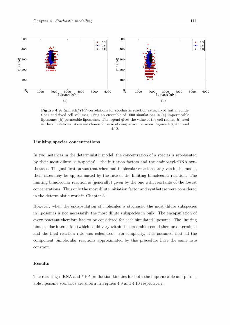
Chapter 4. Stochastic modelling 111
(a) (b)
Figure 4.8: Spinach/YFP correlations for stochastic reaction rates, fixed initial condi-tions and fixed cell volumes, using an ensemble of 1000 simulations in (a) impermeableliposomes (b) permeable liposomes. The legend gives the value of the cell radius, R, usedin the simulations. Axes are chosen for ease of comparison between Figures 4.8, 4.11 and
4.12.
Limiting species concentrations
In two instances in the deterministic model, the concentration of a species is represented
by their most dilute ‘sub-species’ – the initiation factors and the aminoacyl-tRNA syn-
thetases. The justification was that when multimolecular reactions are given in the model,
their rates may be approximated by the rate of the limiting bimolecular reaction. The
limiting bimolecular reaction is (generally) given by the one with reactants of the lowest
concentrations. Thus only the most dilute initiation factor and synthetase were considered
in the deterministic work in Chapter 3.
However, when the encapsulation of molecules is stochastic the most dilute subspecies
in liposomes is not necessarily the most dilute subspecies in bulk. The encapsulation of
every reactant therefore had to be considered for each simulated liposome. The limiting
bimolecular interaction (which could vary within the ensemble) could then be determined
and the final reaction rate was calculated. For simplicity, it is assumed that all the
component bimolecular reactions approximated by this procedure have the same rate
constant.
Results
The resulting mRNA and YFP production kinetics for both the impermeable and perme-
able liposome scenarios are shown in Figures 4.9 and 4.10 respectively.

Chapter 4. Stochastic modelling 112
(a) (b)
(c) (d)
Figure 4.9: The effect of stochasticity in both initial species copy numbers and reactionrates on kinetics in impermeable liposomes, showing (a) mRNA production kinetics (b)YFP production kinetics (c) mRNA Fano factor evolution (d) YFP Fano factor evolution.
The legend gives the value of the cell radius, R, used in the simulations.
By comparison with Figures 4.6 and 4.7 it is clear that the noise strength in both mRNA
and protein production is dramatically increased when stochasticity in species encapsu-
lation is taken into account. This is especially apparent when R = 0.3 µm, where the
Fano factor for Spinach production reaches over two orders of magnitude higher than
when initial concentrations were fixed. This is partially due to the fact that the Fano
factors no longer remain constant in time; instead they increase quasi-linearly during the
expression period. This is because variation in the initial concentrations of reagents biases
the production capacity of each liposome for the entire simulation, so the discrepancies
within an ensemble grow over time.
Another key observation is that while the mean trajectories are comparable to the de-
terministic result when R = 0.8 µm, as R is reduced the mean trajectories for YFP
production tend towards zero. This is explained by the number of initiation factor and
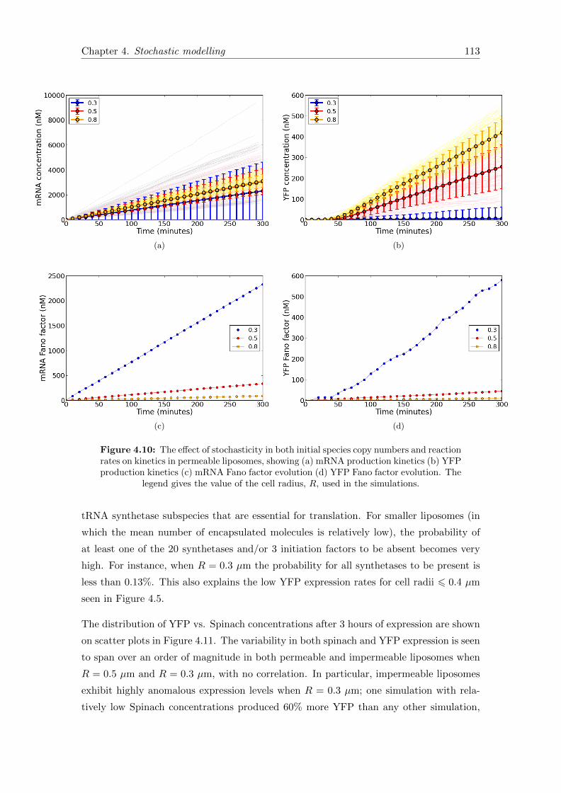
Chapter 4. Stochastic modelling 113
(a) (b)
(c) (d)
Figure 4.10: The effect of stochasticity in both initial species copy numbers and reactionrates on kinetics in permeable liposomes, showing (a) mRNA production kinetics (b) YFPproduction kinetics (c) mRNA Fano factor evolution (d) YFP Fano factor evolution. The
legend gives the value of the cell radius, R, used in the simulations.
tRNA synthetase subspecies that are essential for translation. For smaller liposomes (in
which the mean number of encapsulated molecules is relatively low), the probability of
at least one of the 20 synthetases and/or 3 initiation factors to be absent becomes very
high. For instance, when R = 0.3 µm the probability for all synthetases to be present is
less than 0.13%. This also explains the low YFP expression rates for cell radii 6 0.4 µm
seen in Figure 4.5.
The distribution of YFP vs. Spinach concentrations after 3 hours of expression are shown
on scatter plots in Figure 4.11. The variability in both spinach and YFP expression is seen
to span over an order of magnitude in both permeable and impermeable liposomes when
R = 0.5 µm and R = 0.3 µm, with no correlation. In particular, impermeable liposomes
exhibit highly anomalous expression levels when R = 0.3 µm; one simulation with rela-
tively low Spinach concentrations produced 60% more YFP than any other simulation,
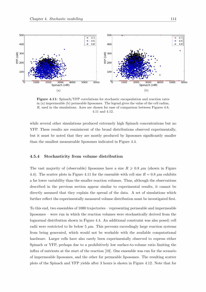
Chapter 4. Stochastic modelling 114
(a) (b)
Figure 4.11: Spinach/YFP correlations for stochastic encapsulation and reaction ratesin (a) impermeable (b) permeable liposomes. The legend gives the value of the cell radius,R, used in the simulations. Axes are chosen for ease of comparison between Figures 4.8,
4.11 and 4.12.
while several other simulations produced extremely high Spinach concentrations but no
YFP. These results are reminiscent of the broad distributions observed experimentally,
but it must be noted that they are mostly produced by liposomes significantly smaller
than the smallest measureable liposomes indicated in Figure 4.4.
4.5.4 Stochasticity from volume distribution
The vast majority of (observable) liposomes have a size R > 0.8 µm (shown in Figure
4.4). The scatter plots in Figure 4.11 for the ensemble with cell size R = 0.8 µm exhibits
a far lower variability than the smaller reaction volumes. Thus, although the observations
described in the previous section appear similar to experimental results, it cannot be
directly assumed that they explain the spread of the data. A set of simulations which
further reflect the experimentally measured volume distribution must be investigated first.
To this end, two ensembles of 1000 trajectories – representing permeable and impermeable
liposomes – were run in which the reaction volumes were stochastically derived from the
lognormal distribution shown in Figure 4.4. An additional constraint was also posed; cell
radii were restricted to lie below 5 µm. This prevents exceedingly large reaction systems
from being generated, which would not be workable with the available computational
hardware. Larger cells have also rarely been experimentally observed to express either
Spinach or YFP, perhaps due to a prohibitively low surface-to-volume ratio limiting the
influx of nutrients at the start of the reaction [10]. One ensemble was run for the scenario
of impermeable liposomes, and the other for permeable liposomes. The resulting scatter
plots of the Spinach and YFP yields after 3 hours is shown in Figure 4.12. Note that for
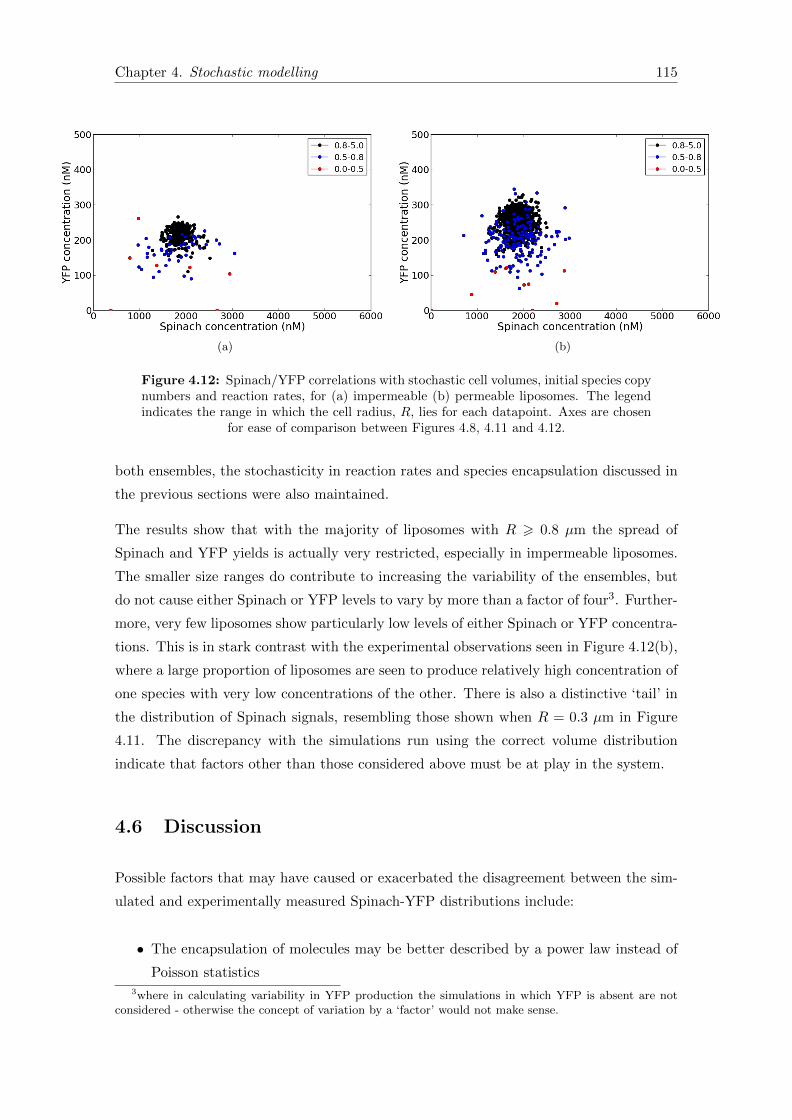
Chapter 4. Stochastic modelling 115
(a) (b)
Figure 4.12: Spinach/YFP correlations with stochastic cell volumes, initial species copynumbers and reaction rates, for (a) impermeable (b) permeable liposomes. The legendindicates the range in which the cell radius, R, lies for each datapoint. Axes are chosen
for ease of comparison between Figures 4.8, 4.11 and 4.12.
both ensembles, the stochasticity in reaction rates and species encapsulation discussed in
the previous sections were also maintained.
The results show that with the majority of liposomes with R > 0.8 µm the spread of
Spinach and YFP yields is actually very restricted, especially in impermeable liposomes.
The smaller size ranges do contribute to increasing the variability of the ensembles, but
do not cause either Spinach or YFP levels to vary by more than a factor of four3. Further-
more, very few liposomes show particularly low levels of either Spinach or YFP concentra-
tions. This is in stark contrast with the experimental observations seen in Figure 4.12(b),
where a large proportion of liposomes are seen to produce relatively high concentration of
one species with very low concentrations of the other. There is also a distinctive ‘tail’ in
the distribution of Spinach signals, resembling those shown when R = 0.3 µm in Figure
4.11. The discrepancy with the simulations run using the correct volume distribution
indicate that factors other than those considered above must be at play in the system.
4.6 Discussion
Possible factors that may have caused or exacerbated the disagreement between the sim-
ulated and experimentally measured Spinach-YFP distributions include:
• The encapsulation of molecules may be better described by a power law instead of
Poisson statistics3where in calculating variability in YFP production the simulations in which YFP is absent are not
considered - otherwise the concept of variation by a ‘factor’ would not make sense.
Chapter 4. Stochastic modelling 116
• Encapsulated DNA may have a reduced activity level;
• The encapsulation of molecules of different species may not be independent
• The encapsulation of every molecule was assumed to be equally likely;
• Stochasticity in the encapsulation of the energy regeneration system was neglected.
As shown in Figure 4.1, a power-law description of species encapsulation could greatly
enhance the variability in the initial conditions used in simulations [64]. Regardless of lipo-
some size, there is always a long tail in the probability distribution that allows liposomes
to become ‘super-concentrated’ and exhibit exceptionally high levels of gene expression
[45]. Since the variability in smaller liposomes was enhanced by an increased relative
standard deviation in initial concentrations using the Poisson distribution, a similar vari-
ability may be achieved in larger liposomes when a power-law encapsulation distribution
is assumed. This would mean that simulations using the true volume distribution and
power-law encapsulation distributions may be similar to the simulated results in Figure
4.11(b), which showed a good agreement with the experimental data.
By using a dual-gene assay, Zohreh Nourian of the Danelon Lab found that a Poisson dis-
tribution of the two DNA constructs was capable of explaining the observed stochasticity
in protein expression if only ∼ 10% were transcriptionally active [11]. If this was the case,
then the mean number of encapsulated DNA molecules should have been only 10% of
the values used in the above simulations. Lower copy numbers of DNA would lead to an
increase in the fractional variation in DNA concentration and hence an enhancement of
the observed stochasticity in gene expression.
In using the Poisson distribution to model initial species distributions, we also assumed
that encapsulation events are independent. However, it is quite plausible that the encap-
sulation of different species are actually highly correlated. The DNA, E and R solutions
are combined before the lipid swelling process, and binding between molecules such as
RNAP with DNA and initiation factors with ribosomal subunits is very likely. The de-
gree of binding between these species decides the cooperativity with which they are then
encapsulated in liposomes. A high cooperativity (caused by a high proportion of bound
molecules) could lead to a higher likelihood of having liposomes either highly efficient in
transcription/translation or with a very poor efficiency in one or both processes. Neglect-
ing this effect may thus have contributed to the underpredicted variability in simulations.
The encapsulation of any molecule in a given liposome has also been assumed to be
equal. In actual fact, the encapsulation rate may be highly dependent on factors such

Chapter 4. Stochastic modelling 117
as molecular size, shape and charge distribution4 [61]. The mean entrapment of some
species may therefore be significantly lower than has been assumed in these studies, and
hence increase the variability in Spinach and YFP production (using the same principle
discussed in the context of low DNA activity).
Throughout the investigations in this chapter it has also been implicitly assumed that all
reagents involved in energy regeneration are encapsulated in sufficient quantities that ATP
and GTP are not depleted by any process other than incorporation in mRNA molecules.
This is not a justified assumption, since myokinase and nucleoside-diphosphate kinase
have a comparable concentration to tRNA-synthetases in bulk and are therefore among the
most dilute species in the solution. This does not affect the results pertaining to permeable
liposomes, since there the intracellular NTPs are assumed to stay in equilibrium with the
external bulk concentration. In the case of impermeable liposomes, however, increased
variability will be introduced.
In this discussion, an emphasis has been placed on inaccuracies in the modelling of species
encapsulation rather than inaccuracies in the modelling of stochasticity in either the
reaction rates or liposome sizes. This is because inaccuracies in these aspects are unlikely
to (significantly) increase the variability in mRNA and YFP yields.
Approximations in reaction rates appear where compound reactions are used to approx-
imate a number of elementary reactions. In the new PUREfrex model, such instances
occurred in the processes of ribosome-RBS binding and CTP-RNAP binding as well as
NTP and amino acid consumption. However, if one out of the many rates approximated
by a compound reaction is much slower than the others – as is often the case – the inaccu-
racy is minimal (Appendix A.2). Furthermore, the similarity between the Fano factors for
mRNA and YFP production noted in section 4.5.2 (despite far more reactions occurring
in the YFP production process) indicates that the consideration of additional reactions
would not significantly affect the noise intensity of the system as a whole. The Fano fac-
tor was far more dependent on stochasticity in initial species concentrations and liposome
size.
Inaccuracies in the liposome radius measurements would be more likely to increase than
decrease the variability in simulations. The liposomes measured in this project tended to
be smaller on average than those previously observed in the lab (from which the experi-
mental mRNA and YFP distributions were taken). Furthermore, the experimental data
is likely to be biased towards larger liposomes, which would have been easier to measure.
The true volume distribution corresponding to the experimental data in Figure 4.12(b) is
4where encapsulation refers to the entrapment of both molecules present in the swelling solution (DNA,E solution and R solution) and those in the external B solution that diffuse in through the lipid membrane.

Chapter 4. Stochastic modelling 118
therefore likely to be shifted to higher values. Using the same approach to model stochas-
ticity in reaction rates and initial conditions as was used in the above investigations,
therefore, variability in the simulation data would be reduced if the liposome sizes were
‘corrected’.
Different approaches to model membrane permeability also would not significantly increase
the variability observed in simulations. Both extremes of permeable and impermeable
liposomes were investigated in this chapter, and the difference in Spinach and YFP yields
between the two scenarios were minimal compared to the standard deviations of the data
(Figure 4.12). Any intermediate degree of permeability would simply lie between the two
extrema, and even stochastic modelling of molecular diffusion events would not produce
a degree of variability greater than that produced by the combination of the data shown
in Figures 4.12(a) and (b). Since the simulations conducted in this project do not show
sufficient variability to match the experimental data, and permeable liposomes produced
noisier kinetics than impermeable liposomes, it may be tempting to conclude that the
experimental liposomes are most likely to be permeable. However, if the encapsulation
rate distribution is modified based on the considerations described in this section it is
possible that the variability in the simulation data may exceed that shown in experiments
and the opposite conclusion may be drawn. It is therefore necessary to improve the
model – at least until the point where the simulation results demonstrate a similar noise
level to that observed in experiments – before conclusions are drawn about membrane
permeability.
4.7 Conclusions and outlook
The stochastic simulations performed in this chapter indicate that stochasticity in reaction
rates has a much lower influence on the noise level in Spinach and YFP production than
cell size or encapsulation statistics. The measured distribution of Spinach and YFP yields
was not reproduced by simulations using cell sizes from experimental data and assuming
Poisson-distributed initial species concentrations. The current hypothesis is that this is
principally due to unfounded assumptions in modelling species encapsulation, such as the
equal likelihood and independence of encapsulation events that led to the adoption of the
Poisson distribution to model the initial species concentrations.
A power-law distribution may be more apt to describe encapsulation statistics, but in order
to investigate this possibility a more quantitative and comprehensive description of the
effect of cell size and reactant concentrations on the parametrisations involved must first be
determined. This could be achieved by fluorescently labelling certain enzymes/reagents in
a number of concentrations, and measuring the encapsulation rate in liposomes of different

Chapter 4. Stochastic modelling 119
sizes. In such an experiment, it may also be found that a completely different distribution
(to either power-law or Poisson) may be a better reflection of reality.
Fluorescently labelling a range of reagents and performing measurements in the above
manner could also reveal biases between the encapsulation rates of different species. Si-
multaneously labelling two reagents using different fluorophores (with minimal crosstalk)
may further reveal cooperativity; the encapsulation rate of DNA and RNAP may be highly
correlated, for example.
More fundamentally, a calibration of the fluorescence data is also necessary for an accurate
data comparison; Figure 4.12(b) has arbitrary units of fluorescence intensity on each axis.
These must be converted to units of concentration in order to obtain the correct x-y scaling
of the experimental distribution. Without this calibration, a range of (vastly different)
experimental results could be claimed to fit the data.
Once the additional experimental data has been achieved, the model should be adjusted
to take the new findings into account. The encapsulation distribution should be mod-
ified (and tailored to different species when appropriate) and the range of simulations
performed during this project should be repeated. Similarities and differences with the
experimental results should then reveal further information about the nature of gene
expression in liposomes.

Chapter 5
Towards gene network modelling
In this chapter the first steps are taken towards modelling the in vitro kinetics of more
complex gene networks. A minimal oscillator based on the circuit by Stricker et al. was
used as the model system [65]. After the creation of the reaction model, parameter values
are estimated based on experimental data from work done both in literature and in the
Danelon lab. The model is then validated based on preliminary experimental results, and
used to assess the feasibility of producing sustained oscillations using this circuit in the
PUREfrex system.
5.1 The minimal oscillator
The model system to be studied is shown in Figure 1.6. Two separate DNA constructs
are used; the ‘oscillator’ construct, and the ‘reporter’ construct. Both are driven by T7
promoters, but also contain LacO operator sites. These are sequences to which dimers of
the LacI protein (native to E. coli) can bind and repress transcription [66]. LacI is coded
for on the oscillator construct, while YFP is coded for on the reporter construct. The
proteins are also tagged with the SsrA peptide that is recognised by ClpXP degradation
proteins [67]. ClpXP and MazF (a protein which cleaves mRNA at ACA, AC and CA
sites [68]), both native to E. coli, are also added to the reaction mixture.
The working principle of the system is that LacI represses its own coding sequence, but
only after a delay (the time taken for transcription, translation, post-translational modifi-
cations and dimerisation). LacI and LacI-coding mRNA transcripts are also constitutively
degraded by ClpXP and MazF respectively. Thus, the LacI concentration should initially
rise until the degree of repression is such that the LacI degradation rate exceeds the
production rate. Then, continued degradation leads to a decreasing LacI concentration,
120

Chapter 5. Towards gene network modelling 121
Figure 5.1: The minimal oscillator, as implemented by the Danelon Lab, consists of twodistinct DNA constructs. The ‘oscillator construct’ (above) expresses SsrA-tagged LacI,while the ‘reporter construct’ (below) expresses SsrA-tagged YFP. Both constructs aredriven by T7 promoters, but are transcriptionally repressed by LacI due to the presence
of LacO sites. The mRNA transcripts also both contain the Spinach sequence.
until the repression of LacI is once again negligible. The concentration of LacI once again
begins to rise, and the cycle is restarted. In this way, sustained oscillations are theoret-
ically achievable using only the oscillator construct. The reporter construct is designed
so that YFP production/degradation matches (or at least is comparable to) that of LacI,
so that oscillation dynamics – if present – can be observed in real-time via fluorescence
spectroscopy.
Unfortunately, the mere presence of the above components is not sufficient to guarantee
that the system will oscillate; the precise balance of the different reaction rates is cru-
cial. In particular, the tightness of repression, non-linearity of rate equations, relative
production/degradation rates and post-translational time delay are key parameters [69].
Increasing repression tightness, non-linearity and time delay favour oscillations, while the
balance of production/degradation rates (relative to the time delay) is somewhat more
complex. They must be sufficient for the LacI concentration to over/undershoot the
steady-state value to such a degree that repression becomes complete/negligible within
each oscillation cycle. In the PUREfrex system, where the maximum yield of mRNA/pro-
tein and hence the expression time appears to be limited, these rates also cannot be too
large. Resource competition with the reporter construct can also add further complexity
to the system dynamics [70].
As a consequence, although the minimal oscillator construct has been made in the lab and
the individual components (repression, production and degradation) have been shown to
be functional, the system has not yet displayed oscillations using the PUREfrex expression
platform. A very similar circuit was however successfully implemented in vivo in E. coli
[65]. Key differences that led to the success probably included the higher transcription,
translation and degradation rates as well as unlimited production yields achievable in vivo
[13, 65, 67, 71, 72].
Chapter 5. Towards gene network modelling 122
Although the use of the in vitro PUREfrex expression system may be inferior to in vivo
alternatives in the above aspects, the major advantage is that the system can be controlled
far more easily. Reaction rates can be modified by the addition of new chemical species,
alteration of existing species concentrations and variation of the buffer conditions, without
fear of killing host cells. In this project, an attempt was made to model the minimal
oscillator system in silico and hence deduce not only why the current circuit is unable to
oscillate, but also what experimental modifications could be made to improve the chances
of creating a successful in vitro oscillating circuit.
5.2 Modelling the minimal oscillator in the PUREfrex sys-
tem
Ideally, a comprehensive model to the level of detail achieved in Chapter 3 would be
used to model the minimal oscillator. This would allow a thorough understanding of
how varying the concentration of each reagent may affect the oscillation dynamics, and
would further permit a stochastic investigation into how feasible it might be to achieve
robust oscillations in liposomes. This would be the next step towards creating a minimal
synthetic cell, capable of executing the more complex behaviour necessary to regulate cell
growth and division, for example.
However, it was found that such a model is neither possible nor desirable with the current
level of knowledge about the system. Even for single-gene expression the final model
derived in Chapter 3 was not entirely satisfactory, particularly regarding protein dynamics.
Many of the additional interactions in the two-gene oscillator construct – such as LacI
dimerisation and MazF-mediated mRNA degradation – have not yet been well quantified,
and would introduce additional unknowns to the system [67, 68]. The quality of the
experimental data needs to be improved quite substantially before a mass-action model
could be regarded with a high level of confidence.
Instead, it was decided to use a much higher-level, coarser-grained approach to model
the minimal oscillator. The level of detail in the model was tuned to match the quality
and quantity of the available experimental data; this approach is similar to that taken by
Karr et al. in a highly-regarded attempt to model the entirety of intracellular processes
in the bacterium Mycoplasma genitalium [73]. Furthermore, key features of the system
that were likely to have a substantial effect on the dynamics (such as resource-sharing
between the two DNA constructs) were rigorously treated, while small details (such as
the distinction between species RNAPb, RNAPc and RNAPd in Chapter 3) were neglected.
As a consequence of this abstraction, only a deterministic model was investigated. The

Chapter 5. Towards gene network modelling 123
loss of detail meant that in a stochastic simulation the stochasticity in the approximated
reaction rates would likely be substantially misestimated (as shown in Appendix A.2).
In this approach, the problem was modularised into focusing on six distinct processes:
• Transcription (of both DNA constructs);
• Translation (of both proteins);
• Post-translational maturation of both proteins
• LacI repression, also accounting for prerequisite multimerisation
• mRNA degradation
• Protein degradation
Initially, the reaction equations were formulated without considering resource sharing.
They were then modified to account for the effects of shared resources (including RNAPs,
ribosomes, and degradation enzymes as well as NTPS and amino acids/tRNAs) at the
end. These topics are dealt with in detail in the following sections.
5.2.1 Simplified transcription and translation modelling
In Chapter 3, transcription and translation were modelled to a very high level of detail.
Many features, however, were important primarily for the stochastic work presented in
Chapter 4. For bulk experiments and deterministic simulations, the details are often
negligible.
As mentioned in Chapter 3.1, a Michaelis-Menten approach for modelling both transcrip-
tion and translation in bulk solution can yield good fit results with high confidence levels
(due to the small number of free fitting parameters). Another advantage of Michaelis-
Menten modelling is that the parameters used have a clear interpretation; Vmax gives
the maximum production rate, and KM is the substrate concentration at which the pro-
duction rate is equal to Vmax/2. This makes it easy to extract these parameters from
experimental kinetics data.
The basic equations for transcription and translation using the Michaelis-Menten approx-
imation are:
∅vP1L−−−→ mL (5.1)
∅vP2L−−−→ L (5.2)
Chapter 5. Towards gene network modelling 124
for the oscillator (LacI) construct and:
∅vP1Y−−−→ mY (5.3)
∅vP2Y−−−→ Y (5.4)
for the reporter (YFP) construct. The species mL and mY represent the LacI- and
YFP-coding mRNA transcripts respectively, while L and Y represent the corresponding
proteins. The rate equations are given by:
vP1i =P1[DNAi]
KM,P1 + [DNAi](5.5)
vP2i =P2[mi]
KM,P2 + [mi](5.6)
(5.7)
where i ∈ {L,Y}. P1 and P2 are the maximum rates for transcription and translation,
with Michaelis constants given by KM,P1 and KM,P2 respectively. The values of these
constants can be related more precisely to the concentrations of the various enzymes and
nutrients involved using the results found in the full model discussed in the preceding
chapters; both Vmax and KM can be easily interpreted from the production curves shown
for example in section 3.7.4. The adaptation of these equations to repressable promoters
will be discussed in section 5.2.4.
The Michaelis-Menten method does not account for transcription or translation stalling,
which is important for assessing the feasibility of oscillations that may have periods lasting
over an hour [65]. The learnings from Chapter 3.5 indicate that transcription stalling is
due to the depletion of CTP, while translation stalling may be due to the build-up of
a toxin during translation which deactivates tRNA. The latter effect was found to ‘cap’
the maximum YFP yield, which did not increase significantly with DNA concentrations
above 1nM (Figure 3.10(b)). Although a dependency on transcription activity has not
been conclusively ruled out, the assumption that translation stalling is purely translation-
dependent will be preserved here (as it was in the preceding chapters).
Thus, the simplest way to model transcription/translation stalling was to cap the maxi-
mum total yields of both mRNA and protein in the system; the total quantity of mRNA
and protein produced – summed over the two constructs – could not exceed the theoret-
ical maximum. This was calculated from the limiting NTP concentration in the case of
mRNA, and deduced from experimental data in the case of protein.

Chapter 5. Towards gene network modelling 125
The protein limit was roughly determined from Figure 3.10(b), and found to be approx-
imately 450 nM. The mRNA limit depends on the NTP composition of the two mRNA
constructs, and could in principle vary depending on which gene has the highest mRNA
yield. This issue was neglected in the model, because it introduces considerable complex-
ity and does not lead to important new results – the magnitude of the cap determines
only the end of the expression time, and hence only limits the period length of oscilla-
tions. Further, this cap can be easily increased experimentally by increasing the NTP
concentration in the reaction, so the value chosen in the model is only used to give an
order-of magnitude indication. For this purpose, a value of 3.3 µM (calculated from the
YFP-spinach construct, and experimentally verified as shown in Figure 3.9(b)) was used.
In order to track the total yields of mRNA and protein, it was necessary to create an addi-
tional ‘artificial species’ for each – mRNAtot and Ptot. This is because the concentration of
the ‘true’ mRNA and protein species would be affected by degradation, and a distinction
is also made between the two genes expressed. For the total yields, the cumulative prod-
ucts from the expression of both genes must be summed, and the effect of degradation is
irrelevant. The rate of change of [mRNAtot] and [Ptot] will therefore be equal to the sum
of the production rates for the two mRNA and protein species respectively.
5.2.2 mRNA and protein degradation
The implementation of mRNA and protein degradation in the PUREfrex system was in-
vestigated in detail in two former Master projects in the Danelon lab. Alicia Soler Canton
established that the MazF interferase from E. coli (which cleaves single-stranded RNA
specifically at AC/CA sequence sites) can effectively degrade the mRNA transcript pro-
duced by the reporter construct for at least 100 minutes [68]. The degree of cleavage was
sufficient to inhibit further translation, but unfortunately does not degrade the Spinach
aptamer; this was hypothesised to be due to steric hindrance, since a single-stranded CA
site is known to be present in the structure. Just van der Wolf established that ClpXP
could degrade SsrA-tagged YFP in PUREfrex for over 5 hours [67], depending on the
enzyme concentration. The degradation kinetics for both enzymes were also quantified,
and the results were applied in this project.
The mRNA degradation kinetics were not investigated over a wide range of mRNA and
MazF concentrations, but a reasonably good fit to experimental data was found using a
first order mass-action reaction model (when using a fixed enzyme concentration). This
took the form:
mivD1i−−−→ ∅ (5.8)

Chapter 5. Towards gene network modelling 126
where i ∈{L, Y} and:
vD1i = D1 · [mi] (5.9)
The rate constant D1 is dependent on the concentration of MazF in solution, but the
exact relation is not well known. This is partly due to insufficient experimental data, but
also because the concentration of the (commercially-purified) MazF used in experiments is
given only in enzyme units of U/ µl. In this case, 1 U is defined as the quantity of enzyme
needed to cleave 1 picomole of standard substrate in 10 minutes at 37 ◦C and pH 7.5. Not
enough information was provided to convert this measure into the molar units necessary
for implementing a proper mass-action model. Leaving D1 as a variable parameter in the
model, however, the MazF concentration range used in the lab indicate that D1 could
take values up to approximately 0.15 min−1. This value is based on data fitting made by
Van der Wolf, who found that D1 ≈ 0.06[MazF] min−1, where the concentration of MazF
is given in units of U/µl [21].
Van der Wolf obtained sufficient experimental data to determine that ClpXP-mediated
protein degradation largely followed Michaelis-Menten kinetics. The reaction equation
can thus be represented as follows:
ivD2i−−−→ ∅ (5.10)
where i ∈{L,Y,L∗,Y∗} (immature LacI, immature YFP, mature LacI and mature YFP
respectively), and the rate vD2i may be written as:
vD2i = D2[i]
KM,D2 + [i](5.11)
where D2 is the maximum degradation rate and KM,D2 is the protein concentration at
which the degradation rate is equal to D2/2 (for a given enzyme concentration). By fitting
experimental data, D2 was found to be approximately equal to 1.0·[ClpXP] min−1, where
[ClpXP] is given in nM. KM,D2 was found to equal 1235 nM, which agrees with values
from literature for ClpXP-mediated GFP degradation [74].
A caveat for modelling ClpXP degradation in this way is that a proportion of the protein
concentration seems to be ‘undegradable’ by ClpXP, but the size of this portion is depen-
dent on the ClpXP concentration in the reaction and can range up to 40% of the initial
protein concentration (Figure B.5) [67]. The precise nature and cause of this phenomenon

Chapter 5. Towards gene network modelling 127
is not understood, and hence will not be quantitatively investigated in this project. How-
ever, its consequences must be considered when interpreting the results of the model, and
subsequently assessing the feasibility of achieving genetic oscillations in the system.
5.2.3 Post-translational modifications
Interestingly, it can be proven that it is theoretically impossible to obtain sustained oscilla-
tions in a minimal oscillator if only (repressed) transcription, translation, and degradation
are represented in the model [69]. A post-translational step to produce the active repressor
is necessary to provide enough time delay between signal (the active repressor concentra-
tion) and response (the repression of the repressor gene) and avoid reaching a steady state.
In practice, this ‘step’ may encompass a range of possible processes – including protein
folding, phosphorylation and racemisation – and the overall rate may vary over several
orders of magnitude for different proteins [75].
In the context of oscillations, the most popular method of modelling post-translational
modifications is to add a fixed, finite delay to the translation rate equation [76–78]. The
presence of the premature peptide is thus considered to be inconsequential to the dynamics
of the system. This is not always a valid approximation; if the modification rate is slow
relative to the degradation rate, then a substantial amount of protein may be degraded
before it reaches the active state. This statement is particularly true in the case of ClpXP
degradation, where proteins are targeted due to the presence of a specific sequence (or
‘tag’) at one end of the polymer. In unfolded proteins, the tags are exposed and hence
be more vulnerable to degradation than in fully-folded proteins, where the tags may be
obscured from the external solution due to the conformation of the protein.
For this reason, it was considered necessary to explicitly represent the immature peptide
as an intermediate species for both proteins in the model. A first order (mass-action) rate
equation was used to model the maturation step, effectively assuming that the process
is spontaneous and independent of other species in the system. This is true in the case
of both LacI and YFP, where the folding process is the dominant rate-limiting step and
does not require the assistance of chaperones [13, 79]. Denoting the fully active LacI and
YFP proteins as L* and Y*, the maturation reactions following translation are given by:
L1/τL−−−→ L* (5.12)
Y1/τY−−−→ Y* (5.13)
where the rate constants are given above the reaction arrows. τL and τY thus represent
the time taken for the maturation of LacI and YFP respectively.
Chapter 5. Towards gene network modelling 128
τY is confidently known to be approximately 20 minutes from experiments performed by
the lab, as mentioned in Chapter 3. τL was also measured by Wilson et al. using time-
resolved fluorescence spectroscopy, and was found to equal approximately 40 seconds
[79]. The measurements were made using a similar pH to the PUREfrex buffer, but at
a temperature of 20 ◦C instead of the PUREfrex incubation temperature, 37 ◦C. Since
protein folding is strongly temperature dependent, the delay time may be significantly
longer than 40 seconds at 37 ◦C [75]. This is due to the higher entropy and larger
fluctuations from thermodynamic equilibrium (thought to be represented by the folded
state) at higher temperatures. The particular temperature dependence of the various
molecular interactions involved in protein folding are quite complex, however, so it is
difficult to predict what τL might be precisely at 37 ◦C [80].
Stricker et al. used τL = 70 seconds when modelling their minimal oscillator, and achieved
good agreement with experimental observations at 37 ◦C (in vivo in E. coli). This is
75% slower than the value found by Wilson, but also cannot be applied directly to the
PUREfrex model due to the difference in environmental conditions in vivo and in vitro.
Based on the results by both Wilson and Stricker, a maturation time of between 0.5-5.0
minutes was considered reasonable for the purposes of this project.
5.2.4 LacI repression
In the above discussion, only the folding time was accounted for as a post-translational
modification step for both proteins. In order for LacI to bind to the LacO operator sites on
DNA, however, it must first dimerise. The dimerisation step also takes a finite amount of
time, but the kinetics do not seem to have been quantified in the literature. The binding
reaction has however been reported to be very strong, such that in a purified sample the
concentration of monomeric LacI is negligible relative to that of dimers [67, 81]. For this
reason, it will be assumed that the binding reaction is rapid enough that the dimerisation
time is negligible, especially since the large uncertainty in the folding time would likely
eclipse the possible range in dimerisation time in any case.
Dimerisation is an important consideration when modelling the effect of repression on
mRNA production; the higher the degree of multimerisation required, the more repressor
protein must be produced before the transcription rate is substantially reduced. This is
an important element of the ‘non-linearity’ that is necessary for sustained oscillations to
be possible in genetic circuits [69]. To incorporate the effect of multimerisation in the
model in the simplest manner (introducing a minimal number of new parameters), an
adaptation of the Hill equation is utilised.

Chapter 5. Towards gene network modelling 129
The Hill equation was originally designed to model cooperative binding of ligands to
proteins; in particular, the binding of oxygen to haemoglobin [15]. For a protein with
multiple ligand-binding sites, the probability of a site being occupied is often dependent
on the occupation state of the other states. This phenomenon is known as cooperative
binding [82]. By using a statistical mechanical approach, it can be shown that the average
fraction of ligand sites that are occupied, θ, is given by:
θ =[Lig]n
KnD + [Lig]n
(5.14)
where [Lig] represents the ligand concentration, KD is the dissociation constant and n
is known as the Hill coefficient, and characterises the cooperativity of the ligands. Non-
cooperative binding is represented by n = 1, positively cooperative binding (in which
binding of a ligand increases the protein molecule’s affinity for further binding) is repre-
sented by n > 1 and conversely negatively cooperative binding is represented by n < 1.
A derivation of the equation may be found in [15].
For LacI-DNA binding the situation is not too dissimilar to ligand-protein binding, since
the LacO sequence is effectively a LacI-binding site on the DNA molecule [76]. We can
therefore straightforwardly apply the Hill equation to find the expected fraction of re-
pressed DNA constructs under the following assumptions:
• There is only one LacO site on each DNA construct
• LacI forms dimers, but no higher order multimers
• The dimerisation reaction is rapid
• Repression is not ‘leaky’ – i.e. if a LacO site is bound, the downstream gene is not
transcribed.
Neither of the first two assumptions are true, but they are reasonable approximations
based on experimental data. Firstly, though figure 5.1 shows that two LacO sites are
present on the oscillator construct, in lab experiments no significant difference has been
seen (in terms of repression efficiency) relative to the same construct lacking the upstream
LacO site. The presence of the upstream LacO sequence can thus be neglected in the
model, such that each DNA molecule contains a single LacI binding site.
Secondly, LacI forms two different possible multimers: dimers and tetramers. However,
the binding affinity to LacO is not significantly different for the two species [81]. Only

Chapter 5. Towards gene network modelling 130
the formation of dimers is therefore necessary for LacO binding, and tetramerisation may
be neglected1.
The third assumption is necessary to express the concentration of LacI dimers in terms
of the concentration of monomers. If the dimerisation reactions are sufficiently rapid, an
equilibrium is reached and the concentration of dimers is proportional to [L]2 (shown in
Appendix A.4). The constant of proportionality is the association constant of dimerisa-
tion, KA, which is known to be very large [81].
The final assumption of tight repression means that the overall transcription rate can be
linearly scaled proportional to the fraction of unbound LacO sites calculated from the Hill
equation. By substituting n = 1 and [Lig]= KA[L]2 in equation 5.14 we can write the
fraction of bound LacO sites as:
θLacO =[L]2
Kα + [L]2(5.15)
where Kα = KDKA
.
Thus the transcription rate equations (5.5) discussed in section 5.2.1 only need to be
multiplied by (1-θLacO) to incorporate repression, introducing just a single new fitting
parameter, kα. KD is the dissociation constant for LacI-LacO binding, and has been
experimentally measured; the dissociation rate is typically 4 orders of magnitude lower
than the association rate for nanomolar concentrations of the two species, so KD is almost
vanishingly small [66]. This would appear to indicate that only a minute quantity of
LacI is necessary to fully repress transcription in the system. This is however incorrect,
because competition between different macromolecules for a common pool of ligands is
not considered in the derivation of the Hill equation. In practice, the LacI concentration
[L] must at least equal the DNA concentration in order to repress all constructs in the
reaction solution. A more appropriate lower bound for Kα can be obtained by using this
fact, since Kα is equal to the concentration of dimers necessary to repress 50% of the
DNA molecules. The minimum value of Kα is thus approximately equal to [DNAi]/2 for
the ith DNA construct, where i ∈ {L,Y}.
5.2.5 Resource sharing
The above discussion on the Hill equation highlights the importance of considering re-
source sharing in the formulation of the reaction equations. In fact, all of the equations
1Tetramerisation would still affect the equilibrium concentrations of LacI monomers and dimers, butin the absence of experimental data for the (relative) rate constants of dimerisation and tetramerisationthis effect was neglected.
Chapter 5. Towards gene network modelling 131
presented above for transcription, translation and degradation must be modified to ac-
count for competition between molecules for a common pool of enzymes2.
Standard Michaelis-Menten kinetics, for instance, assume that the enzyme catalyses only
one reaction. When an enzyme may catalyse multiple reactions the different substrates
competitively inhibit each other, so applying the standard Michaelis-Menten rate equation
3.4 to each reaction gives an overestimate for the actual rates. Instead, the equation for
the ith substrate should be modified to:
vi = Vmax[Si]
KMi
(1 +
∑j
[Sj ]KDj
)+ [Si]
(5.16)
where KM is the Michaelis constant KM = kr+kcatkf
and KD is the dissociation constant
KD = krkf
, using the terminology from equation 3.2 [83]. Subscript i and j label the
different substrate species and their respective rate constants, and the sum over j runs
over the competing substrates.
In the minimal oscillator system, there are two competing substrates for each Michaelis-
Menten reaction; the two different DNA constructs compete for RNAP, the two mRNA
transcripts compete for both ribosomes and MazF, and the two proteins compete for
ClpXP. If it is assumed that the competing substrates for each enzyme all have the same
dissociation constant (which is reasonable given that the binding sites are the same for
each substrate) and that kcat << kr, as was found in Chapter 3.7.4, equation 5.16 reduces
to:
vi = Vmax[Si]
KMi ([Sj ] + [Si])(5.17)
where no sum is necessary because there is only one competing species, and {i, j} ∈ {L, Y }.
This treatment does not apply to enzymatic degradation of mRNA, however, which was
modelled using the first order rate equation 5.9. In this case, assuming the two mRNA
transcripts have the same affinity for MazF, competition can be accounted for simply by
scaling the degradation rate for each substrate proportionally to their relative concentra-
tions. This is equivalent to assuming that MazF molecules are evenly distributed among
all mRNA transcripts (and hence the effective concentration of MazF for each substrate
is reduced), and degrades each transcript at the same rate. The latter assumption is
2The competition for ‘consumables’, NTPs and tRNAs, are already accounted for by capping transcrip-tion and translation as described in section 5.2.1. Competition for amino acids is not explicitly consideredbecause experimental results from Chapters 2 and 3 indicate that tRNAs are depleted first, and are hencethe limiting resource in translation.

Chapter 5. Towards gene network modelling 132
convenient but not necessarily true, since it depends on the number of (and environment
around) AC/CA sequence sites on the substrates.
Competition for LacI on LacO operator sites is also present, which gives a lower bound
for Kα as discussed in section 5.2.4. Since Kα is the only parameter affected by this
competition, even the presence of the (neglected) upstream LacO site on the oscillator
construct can be implicitly accounted for in fitting this parameter to the data.
5.3 Final oscillator model presentation
Taking all of the above into account, the final model for the minimal oscillator is as follows:
∅vP1L−−−⇀↽−−−vD1L
mL (5.18)
∅vP1Y−−−⇀↽−−−vD1Y
mY (5.19)
∅vP2L−−−⇀↽−−−vD2L
L (5.20)
∅vP2Y−−−⇀↽−−−vD2Y
Y (5.21)
LvL−→ L∗ vD2L∗−−−−→ ∅ (5.22)
YvY−−→ Y∗ vD2Y ∗−−−−→ ∅ (5.23)
with rate equations given by:
Chapter 5. Towards gene network modelling 133
vP1i = θi · P1[DNAi]
KM,P1 + [DNAi] + [DNAj ](5.24)
vP2i = P2[mi]
KM,P2 + [mi] + [mj](5.25)
vi =1
τi[i] (5.26)
vD1i = D1 · [mi] ·[mi]
[mi] + [mj](5.27)
vD2i = D2[i]
KM,D2 + [i] + [j] + [i∗] + [j∗](5.28)
vD2i∗ = D2[i∗]
KM,D2 + [i] + [j] + [i∗] + [j∗](5.29)
(5.30)
where {i, j} ∈ {L, Y} represent the species from the competing constructs and
θi =Kαi
Kαi + [L]2(5.31)
is 1−θLacO calculated in section 5.2.4, representing the fraction of unrepressed genes from
construct i. The estimated ranges of the various parameters that may be achievable in
the Danelon Lab at the present time are given below in Table 5.1.
These estimates were based on both data from literature (including lab publications)
and experimental data described in Chapter 3.7. Upper bounds for P1 and P2 were
calculated based on adjustable RNAP/ ribosome/ initiation factor concentrations up to
Table 5.1: Estimated range of parameter values for the minimal oscillator model, de-termined as described in the text.
Parameter Estimated range Source
P1 < 12 nM min−1 [13], ibid.KM,P1 1.7− 3.1 nM [13], ibid.P2 < 4 nM min−1 [13], ibid.KM,P2 30− 80 nM [13], ibid.τL 1.0− 5.0 min [65, 79]τY 21.7 min [13, 38]D1 < 0.15 min−1 [21, 68]D2 < 130 nM min−1 [67]KM,D2 1100− 1300 nM [67, 74]KαL > [DNAL]/2 –KαY > [DNAY ]/2 –
Chapter 5. Towards gene network modelling 134
the standard concentrations used in PUREfrex, those for D1 and D2 are based on the
maximum MazF/ClpXP concentrations tested in the lab thus far. These rate constants
may therefore exceed the apparent upper limits shown in the table if larger concentrations
of these enzymes are added to the reaction solution, but since this region of the parameter
space has not been well-explored experimentally it was not included in the estimated
range. The ‘true’ upper limits for these parameters are governed by the stock enzyme
concentrations, and the buffer they are stored in; only a limited volume of each enzyme
may be added to the reaction to avoid dilution of the other necessary reagents.
As discussed in section 5.2, the transcription and translation rates should go to zero as
the NTPs and tRNAs deplete. The easiest way to implement this was to model P1 and
P2 as step functions, taking a constant value (within the estimated range given in Table
5.1) before dropping discontinuously to zero when the relevant substrate has depleted.
5.4 Software selection
Wolfram Mathematicar was chosen as the modelling platform for solving the above system
of equations, for similar reasons to those given in Chapter 3.7.1. Namely, it is a powerful
and flexible software package capable of numerically solving complex differential equations
(such as those presented by the numerous complex rate equations in this model) efficiently.
Function definitions such as those required for P1 and P2 can also be created easily and
handled smoothly in conjunction with the differential solver.
The defining tool that favoured the use of Mathematica over similar competitors such as
Maple and Matlab is the Manipulate interface (Figure 3.6) described earlier, which allows
large multidimensional parameter spaces to be explored with ease. Since the aim of this
part of the project was to identify regions of the parameter space capable of supporting
oscillations, the efficiency afforded by this function was invaluable.
5.5 Model validation
At the time of writing, limited experiments have been performed with the full minimal
oscillator network. The data that has been produced explores a very limited parameter
space, and does not exhibit any oscillatory behaviour (Figure 5.2). Spinach and YFP
fluorescence signals were measured to track the concentrations of mRNA and YFP in real
time, but due to the inability for MazF to consistently cleave the Spinach aptamer only
the YFP signal could be interpreted reliably. Furthermore, fluorescence intensity was
measured using the Clariostar plate reader, which has been shown to give highly variable
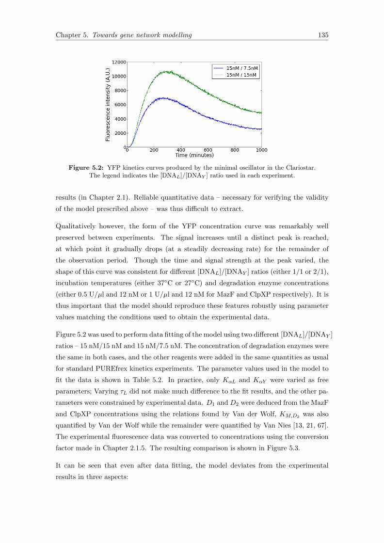
Chapter 5. Towards gene network modelling 135
Figure 5.2: YFP kinetics curves produced by the minimal oscillator in the Clariostar.The legend indicates the [DNAL]/[DNAY ] ratio used in each experiment.
results (in Chapter 2.1). Reliable quantitative data – necessary for verifying the validity
of the model prescribed above – was thus difficult to extract.
Qualitatively however, the form of the YFP concentration curve was remarkably well
preserved between experiments. The signal increases until a distinct peak is reached,
at which point it gradually drops (at a steadily decreasing rate) for the remainder of
the observation period. Though the time and signal strength at the peak varied, the
shape of this curve was consistent for different [DNAL]/[DNAY ] ratios (either 1/1 or 2/1),
incubation temperatures (either 37◦C or 27◦C) and degradation enzyme concentrations
(either 0.5 U/µl and 12 nM or 1 U/µl and 12 nM for MazF and ClpXP respectively). It is
thus important that the model should reproduce these features robustly using parameter
values matching the conditions used to obtain the experimental data.
Figure 5.2 was used to perform data fitting of the model using two different [DNAL]/[DNAY ]
ratios – 15 nM/15 nM and 15 nM/7.5 nM. The concentration of degradation enzymes were
the same in both cases, and the other reagents were added in the same quantities as usual
for standard PUREfrex kinetics experiments. The parameter values used in the model to
fit the data is shown in Table 5.2. In practice, only KαL and KαY were varied as free
parameters; Varying τL did not make much difference to the fit results, and the other pa-
rameters were constrained by experimental data. D1 and D2 were deduced from the MazF
and ClpXP concentrations using the relations found by Van der Wolf, KM,D2 was also
quantified by Van der Wolf while the remainder were quantified by Van Nies [13, 21, 67].
The experimental fluorescence data was converted to concentrations using the conversion
factor made in Chapter 2.1.5. The resulting comparison is shown in Figure 5.3.
It can be seen that even after data fitting, the model deviates from the experimental
results in three aspects:

Chapter 5. Towards gene network modelling 136
Table 5.2: The model parameters used to fit the experimental data in Figure 5.3, wherevalues for [DNAL] and [DNAR] are given in the figure legend. The estimated fitting range
from Table 5.1 is also shown for reference.
Parameter Estimated range Fitted value
P1 < 12 nM min−1 12 nM min−1
KM,P1 1.7− 3.1 nM 2.4 nMP2 < 4 nM min−1 4 nM min−1
KM,P2 30− 80 nM 50 nMτL 1.0− 5.0 min 2 minτY 21.7 min 21.7 minD1 < 0.15 min−1 0.03 min−1
D2 < 130 nM min−1 12 nM min−1
KM,D2 1100− 1300 nM 1235 nMKαL > [DNAL]/2 [DNAL]/2KαY > [DNAY ]/2 [DNAY ]/2
1. The height of the modelled YFP peaks are significantly higher than those found
experimentally;
2. The peaks occur earlier in the model than they do in experiments;
3. The YFP concentration gradually decays to a finite (non-negligible) value in exper-
iments, but it decays rapidly to zero in the model;
4. While the curves are smooth in the experimental data, there is a kink in the model
curves (just before the rapid decay phase).
The first point can be explained by the uncertainty in the calibration used to convert flu-
orescence data to YFP concentration in the experimental data. Based on the experiences
in gathering standard kinetics data from the Clariostar (described in Chapter 2.1.6), it
has been seen that the calibration frequently underestimates the true fluorophore concen-
trations by more than a factor of two. In this sense, it is not surprising that the vertical
scaling of the experimental data does not match that of the model, and it is probable that
the model predictions are more correct.
The explanation for the next two points are linked – they are both related to the charac-
terisation of enzymatic degradation. While MazF is only confidently known to be active
for the first ∼ 2 hours, and ClpXP is known to be active for up to ∼ 5 hours3, the data in
Figure 5.3 runs for 16 hours and 40 minutes. The quantification of the degradation rates
is therefore only strictly valid in the very early stages of the expression curve; beyond 120
minutes, the degradation rates are unknown and quite possibly lower than those assumed
3By these timepoints, the substrates used in the activity assays for MazF and ClpXP had depleted.

Chapter 5. Towards gene network modelling 137
Figure 5.3: Fit of the YFP kinetics curves produced by the oscillator model to theexperimental data shown in Figure 5.2. The parameters used in the model to make thefit are given in Table 5.2. Arbitrary fluorescence units of the experimental data wereconverted to YFP concentrations using the conversion factor calculated in Chapter 2.1.5.
The legend indicates the [DNAL]/[DNAY ] ratio used in each experiment.
in the model. It is fully conceivable that this discrepancy would cause a mismatch of the
model to the data.
Let us consider, as an ‘extreme’ possibility, a model in which mRNA degradation rate
drops (discontinuously) to zero after two hours. The new model results are shown in Figure
5.4. The YFP peak is clearly seen to be shifted to the right, more closely matching the
experimental data. The kink in the curves at 120 minutes corresponds to the discontinuous
halt of mRNA degradation at this time. In practice, the loss of MazF activity would be
more gradual and hence create a smoother curve that can match the experimental data.
The slowdown of mRNA degradation over time could thus explain the discrepancy in the
second point.
The neglect of a similar slowdown in YFP degradation (due to ClpXP deactivation) in the
model could explain the discrepancy in the signal curves during the degradation phase.
While the model assumes that the same degradation rate is maintained throughout the
observation period, it may in fact slow down and hence cause the shallower degradation
curve in experimental data. The quantity of ‘undegradable’ protein is also neglected in
the model, while experiments have shown that between 16-35% of the protein may be
undegradable with this ClpXP concentration (Figure B.5). This could explain why the
experimental curves ‘plateau’ at a finite YFP concentration, whereas the model curves
degrade completely within the same time frame.
The kink in the model curves just before the rapid decay phase is because tRNA depletion
has been assumed to cause translation to stall abruptly after 450 nM of protein has been
produced. After this point, only protein degradation takes place, which explains the
subsequent rapid decay. The kinks seen in Figures 5.3 and 5.4 are an unphysical artefact

Chapter 5. Towards gene network modelling 138
Figure 5.4: A comparison of the oscillator model with experimental data where allMazF is assumed to deactivate abruptly after 2 hours. The model and experimental dataare otherwise identical to Figure 5.3. The legend indicates the [DNAL]/[DNAY ] ratio
used in each experiment.
of this approximation, since in practice the translation rate smoothly drops to zero as the
maximum protein yield is approached (as seen in Figure 3.10).
The above discussions provide an explanation for the discrepancies between the model and
the experimental data. They indicate that the model is inaccurate after approximately
two hours, after which the activity of MazF is not known. Before this point however, the
model should be ‘good enough’ to provide an indication of the plausibility of achieving
oscillations with a period of less than 1 hour.
5.6 Model predictions
The parameter space defined by the parameter ranges in Table 5.1 was subsequently
scanned using Wolfram Mathematica in order to determine what regions – if any – might
support oscillations4. This process was aided by the fact that it is already known from
literature that τL should be maximised while KαL and KαY should be minimised to favour
oscillations [69, 78]. These values were therefore set at their maximum and minimum
values in their respective ranges throughout the scanning process. Further, the range of
KM,D2 values was quite small and high above the maximum protein yield, so variation in
this parameter does not much affect the dynamics of the system. The YFP maturation
time τY also does not affect the oscillatory dynamics of the system at all.
4Analytical methods to determine unstable fixed points of the system of equations were also attemptedusing Mapler. Unfortunately, the equations were very unwieldy to work with - the expressions for theeigenvalues of the system were extremely large, containing over 50 terms each. Due to time constraints,this ‘searching’ method using Mathematica was therefore employed instead.
Chapter 5. Towards gene network modelling 139
Only the production and degradation parameters P1, KM,P1 , P2, KM,P2 , D1 and D2 as
well as the relative concentrations of the two DNA constructs were therefore varied. All
but one of the parameters was held fixed, while one was varied. The fixed values for
KM,P1 and KM,P2 were in the middle of their respective ranges (the average value found
from experiments) while the production and degradation parameters were fixed at their
maximum values (the values relevant to standard PUREfrex reagent concentrations). The
DNA concentrations were set to 1 nM each (compared to 15 nM each in the experimental
data discussed above) to extend the expression time.
Unfortunately, no oscillations were observed anywhere in the parameter space. At this
point, further research was conducted in the literature to seek methods to manipulate the
system into producing oscillations. It was found that zeroth-order protein degradation
– corresponding to a very low value for KM,D2 – greatly enhances the robustness of
oscillations and thus enlarges the parameter space in which they can be found [84]. It was
also found that ClpXP degradation follows zeroth-order kinetics in E. coli, and Stricker
et al. used a very low KM,D2 value to model ClpXP degradation in their successful in vivo
version of the minimal oscillator [65, 84].
Conversely, KM,D2 was determined to be more than two times the maximum protein yield
when using ClpXP in the PUREfrex system, leading to first order degradation kinetics.
This was hypothesised as a possible (partial) cause for the lack of oscillations. The cause
for the lower affinity between ClpXP and SsrA-tagged substrates in vitro as opposed to in
vivo was found to be the lack of SspB adaptor protein. SspB can bind both SsrA peptide
tags and ClpXP, and hence increase the affinity of the two molecules. The addition of
SspB in vitro can decrease KM,D2 by two orders of magnitude, from ∼1100 nM down to
15 nM at 30 ◦C [74]. SspB is currently being purified by the Danelon Lab to investigate its
effectiveness under PUREfrex buffer conditions, but (at the time of writing) its activity
is still yet to be tested. For the purposes of this in silico study, it will be assumed that
in the presence of SspB KM,D2 can reach 15 nM.
Considering zeroth-order protein production and degradation rates5, Mather et al. found
that maximising both the production and degradation rates favoured oscillatory behaviour
for minimal oscillators [76]. Although protein production in the PUREfrex system is
certainly not zeroth order, the possibility of enhancing the protein production rate was
also explored. In the PURExpress system, the protein production rate can be up to
ten times higher than in PUREfrex. It may therefore be postulated that by varying
the concentrations of enzymes involved in the translation process, it may be possible to
increase the translation rate in PUREfrex by a factor of ten.
5As well as using a Hill function to represent repression.

Chapter 5. Towards gene network modelling 140
Figure 5.5: Damped oscillations in the minimal oscillator, assuming an increased trans-lation rate and ClpXP-SsrA affinity. The kink at minute 190 is due to tRNA depletion.
Parameter values are given in Table 5.3.
Using the now-extended parameter space, damped oscillatory behaviour with a period of
∼ 65 minutes were obtained (Figure 5.5). The final parameters are given in Table 5.3.
These were the most sustained oscillations that could be found in the parameter space
with a period of less than one hour.
As expected, in order to produce these oscillations it was beneficial to maximise P1, P2, τL
and D1, and minimise KαL and KM,D2 . The most ‘unrealistic’ of the parameter choices
was P2, which was ten times larger than the maximum value in a standard PUREfrex
reaction. It was however found that (weaker-amplitude) oscillations were also achievable
Table 5.3: The model parameters used to produce damped oscillations in Figure 5.5.The estimated fitting range from Table 5.1 is modified to account for the potential ofPURExpress to increase the translation rate P2 and the potential of SspB to increase the
affinity of ClpXP to SsrA-tagged substrates (and hence decrease KM,D2).
Parameter Estimated range Fitted value
P1 < 12 nM min−1 12 nM min−1
KM,P1 1.7− 3.1 nM 2.4 nMP2 < 40 nM min−1 40 nM min−1
KM,P2 30− 80 nM 50 nMτL 1.0− 5.0 min 5 minτY 21.7 min 21.7 minD1 < 0.15 min−1 0.15 min−1
D2 < 130 nM min−1 4.8 nM min−1
KM,D2 15− 1300 nM 15 nMKαL > [DNAL]/2 [DNAL]/2KαY > [DNAY ]/2 [DNAY ]/2 + 2 nM[DNAL] < 250 nM 1 nM[DNAY ] < 250 nM 1 nM
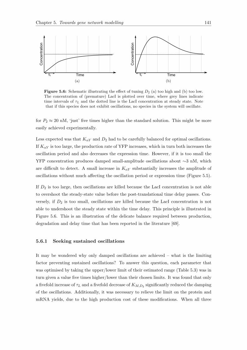
Chapter 5. Towards gene network modelling 141
Time
Concentration
τL
(a)
Time
Concentration
τL
(b)
Figure 5.6: Schematic illustrating the effect of tuning D2 (a) too high and (b) too low.The concentration of (premature) LacI is plotted over time, where grey lines indicatetime intervals of τL and the dotted line is the LacI concentration at steady state. Notethat if this species does not exhibit oscillations, no species in the system will oscillate.
for P2 ≈ 20 nM, ‘just’ five times higher than the standard solution. This might be more
easily achieved experimentally.
Less expected was that KαY and D2 had to be carefully balanced for optimal oscillations.
If KαY is too large, the production rate of YFP increases, which in turn both increases the
oscillation period and also decreases the expression time. However, if it is too small the
YFP concentration produces damped small-amplitude oscillations about ∼3 nM, which
are difficult to detect. A small increase in KαY substantially increases the amplitude of
oscillations without much affecting the oscillation period or expression time (Figure 5.5).
If D2 is too large, then oscillations are killed because the LacI concentration is not able
to overshoot the steady-state value before the post-translational time delay passes. Con-
versely, if D2 is too small, oscillations are killed because the LacI concentration is not
able to undershoot the steady state within the time delay. This principle is illustrated in
Figure 5.6. This is an illustration of the delicate balance required between production,
degradation and delay time that has been reported in the literature [69].
5.6.1 Seeking sustained oscillations
It may be wondered why only damped oscillations are achieved – what is the limiting
factor preventing sustained oscillations? To answer this question, each parameter that
was optimised by taking the upper/lower limit of their estimated range (Table 5.3) was in
turn given a value five times higher/lower than their chosen limits. It was found that only
a fivefold increase of τL and a fivefold decrease of KM,D2 significantly reduced the damping
of the oscillations. Additionally, it was necessary to relieve the limit on the protein and
mRNA yields, due to the high production cost of these modifications. When all three

Chapter 5. Towards gene network modelling 142
Figure 5.7: Sustained oscillations in the minimal oscillator, using all parameter valuesfrom Table 5.3 except τL=25 minutes and KM,D2=3 nM. Infinite resources are also
assumed.
.
changes were made, sustained oscillations with a period of 100 minutes was achieved6
(Figure 5.7). The long period means that it is also necessary to maintain the activity of
the degradation enzymes for at least ∼4 hours in order to observe the oscillations.
The limiting parameters are not too surprising; zeroth-order protein degradation can only
be achieved if KM,D2 is much less than the average concentration of LacI and YFP, which
was not the case for the damped oscillator, but is the case in the sustained oscillations.
This has been shown experimentally to substantially increase the robustness of oscillations,
as previously discussed [84]. A ‘sufficiently long’ post-translational time delay (τL) has
also mathematically been shown to be crucial for sustained oscillations [69].
Unfortunately, these changes would be very difficult to implement in practice. For the
damped oscillations, it was already assumed that KM,D2 was substantially reduced by the
(as yet unimplemented) addition of SspB to the reaction solution. The folding time for
LacI (approximately equal to τL) may be slowed by increasing the temperature and/or
varying the buffer conditions, but these changes would also affect other rate constants in
ways that are not yet well understood [10, 75].
The condition of unlimited resources may however be implemented relatively easily. In
liposome experiments, resources would be unlimited if the membranes are permeable
(under the definition given in Chapter 4). The permeability of the liposomes produced
in current lab protocols has not been conclusively determined, but if necessary it could
6Sustained oscillations with a very similar profile could also be achieved with only a threefold increasein τL (∼ 15 minutes), but KM,D2 had to lie below∼ 3nM.
Chapter 5. Towards gene network modelling 143
be enhanced by tuning the lipid composition [10]. This could also prevent deactivation of
the degradation enzymes.
Expressing the minimal oscillator in liposomes may have further benefits. If liposomes
are highly crowded (due to a power-law distribution of encapsulation rates, for example)
then the folding time (and hence τL) for LacI may be increased [85]. Additionally, the
broad variability in liposome experiments would allow a wide region of the parameter
space to be sampled simultaneously. The probability for at least one liposome to express
oscillations may therefore be relatively high.
5.7 Summary and outlook
A model was developed for the minimal oscillator construct which was recently experi-
mentally implemented in the Danelon lab. The model was simplified relative to the model
developed in Chapter 3 in order to keep the mathematics of the more complex system
digestible, as well as to minimise the number of free parameters which have not been
experimentally quantified.
As a consequence, the model also involved many more assumptions and approximations
than the previous model. Notable examples include:
• The two DNA constructs are transcribed at the same rate;
• The two mRNA transcripts are translated at the same rate;
• The two mRNA transcripts are degraded by MazF at the same rate;
• The two proteins (in both folded and unfolded form) are degraded at the same rate;
• The LacI dimerisation rate is fast enough to equilibrate on the timescale of LacI-
LacO binding;
• The LacI-LacO (un)binding rate is fast enough to equilibrate on the timescale of
transcription;
• Repression is not leaky;
• The upstream LacO site on the oscillator construct is neglected;
• The transcription/translation rates are independent of the NTP/tRNA concentra-
tion until the maximum ‘cap’ is reached, at which point they stall immediately;
• The limiting NTP concentration is assumed to be CTP, (based on the reporter
construct)

Chapter 5. Towards gene network modelling 144
• The degradation enzymes are assumed to be active for the full duration of the
simulations (up to 1000 minutes long);
• ‘Undegradable proteins’ are neglected.
Similarly to Chapter 3, many of these assumptions were made for convenience, in the
absence of experimental evidence to the contrary.
The inaccuracy of some assumptions were immediately apparent upon fitting experimental
data. The discontinuous drop in the translation rate caused an unphysical kink in the
production curve, which did not match the data. Other discrepancies could be explained
by a reduction in MazF and ClpXP activity over time.
Staying within the parameter space that can be explored using the standard PUREfrex
system kit, it was not possible to obtain oscillations. It was necessary to increase the
affinity of ClpXP to protein substrates by at least two orders of magnitude and increase
the translation rate at least fivefold before damped oscillations could be achieved in the
system. These parameter values could potentially be reached by the use of SspB adaptor
proteins and increasing the concentration of translation factors in the reaction solution,
respectively.
To obtain sustained oscillations, there is an additional requirement that the folding time
for LacI had to be extended to at least 15 minutes, and transcription, translation and
enzymatic degradation activity had to be maintained for at least four hours in order
to observe two concentration peaks. A semi-permeable membrane allowing diffusion of
NTPs and toxins such as X would be necessary to meet the last condition. More direct
experimental data should also be gathered to check the activity of MazF over this time
period.
Running the experiments in liposomes may be able to satisfy both of the above two
necessary requirements, and further allows a wide range of the parameter space to be
sampled simultaneously. In order to observe the oscillations in real-time, however, a
temperature controller capable of maintaining the sample at 37 ◦C while mounted on
the confocal microscope. This functionality exists on the Nikon microscope discussed in
Chapter 2.2, but still remains to be tested. If it proves to be effective, and adjustments
are made to the reaction solutions as recommended above, the probability of observing
oscillating liposomes could be quite high.

Chapter 6
Conclusions & Outlook
In this thesis, progress was made towards answering each of the research questions set out
at the start of the project. Detailed conclusions and suggestions for further work were
provided at the end of each of the preceding chapters, and below highlights of the key
findings will be presented together with some concluding remarks.
6.1 Experimental techniques
6.1.1 Clariostar microplate reader
The Clariostar microplate-reading spectrophotometer was found to be capable of tracking
Spinach and YFP production kinetics in bulk solution, but the data showed a high level
of variability due to condensation formation on the well lids during incubation. For
this reason, the Eclipse cuvette-based spectrophotometer is still recommended if accurate
quantitative data is desired.
Nevertheless, for qualitative data the Clariostar is a more efficient alternative to the
Eclipse. Protocols were developed to both minimise condensation formation and process
the raw data in order to remove artefacts of evaporation effects. A fluorescence intensity
to species concentration calibration was also made, which can give a rough idea of the
mRNA and protein yields and production rates over time.
While I believe it would be difficult to much improve the quality of the data using the
current experimental setup, modifications to the microplates may improve results. Taller,
narrower wells with a smaller surface/volume ratio would reduce the evaporation rate, and
bottom-optic microplates would remove most of the sensitivity to evaporation altogether.
145
Chapter 6. Conclusions and outlook 146
With these changes, the Clariostar may equal or even better the Eclipse for the acquisition
of quantitative data.
6.1.2 Nikon confocal microscope
Appropriate settings for imaging TRITC-labelled liposomes expressing Spinach and YFP
have been determined for the Nikon confocal microscope. The instrument gives a good
image resolution down to the diffraction limit, and the integrated analysis software makes
measuring liposome sizes and fluorescence intensities very straightforward. Unfortunately,
there is a substantial degree of crosstalk from TRITC in the YFP channel when using
the lasers/dichroics currently installed. Measurements of mean YFP intensity should
therefore be made away from the liposome edges to avoid contamination from the TRITC
crosstalk.
A major incentive to use the Nikon instrument is the interface with a super-resolution
SIM instrument, which is theoretically capable of resolving liposomes down to ∼ 500 nm
in diameter. This would approximately halve the current resolution limit, and provide
valuable data for stochastic modelling. Unfortunately, due to time constraints it was not
possible to test the SIM in this project, but this should be considered a priority for the
near-future.
6.2 Model development
A mathematical model was developed that contained sufficient detail to model stochastic
simulations accurately, while also including judicious approximations to minimise the
computational load. Each reaction in the model is scientifically motivated by experimental
evidence, the most important advance being the association of the YFP plateau with
tRNA deactivation during the translation process1.
The rate parameters used in the model were derived from deterministically fitting data
from bulk kinetics experiments run in both the Clariostar and the Eclipse. The reliability
of the fitting procedure was enhanced by the use of educated initial guesses for almost
every parameter, greatly limiting the fitting ranges. However, the reliability of the final
values were also reduced by the relatively poor quality of the experimental data used in
the fitting procedure.
1tRNA deactivation during transcription also has not bee ruled out.

Chapter 6. Conclusions and outlook 147
Regardless, the final model was capable of fitting the vast majority of the data within
reasonable bounds, and predicted the response of the system to a different RNAP concen-
tration and delayed addition of tRNA reasonably well. The most noticeable weakness of
the model was an apparent oversensitivity to tRNA concentration; this could be remedied
by a small alteration to the rate equation for translation.
In order to improve the current model significantly, it is crucial to obtain higher quality
experimental data with lower variability. The first step would be to create a new set of
experimental data (at the same or similar DNA concentrations as those used in Chapter 2)
using only the Eclipse, as opposed to the Clariostar. The parameters derived from fitting
these data would be likely to be much more reliable than the values found in Chapter 3.
6.3 Stochastic modelling
The deterministically validated model was successfully adapted for use in a stochastic
simulator (StochPy). The results of the stochastic simulations indicate that stochasticity
in encapsulation efficiency of the different PUREfrex reagents are the dominant cause
for the large variability and lack of correlation between YFP and Spinach production.
Furthermore, Poisson-distributed encapsulation rates were not sufficient to explain the
experimentally observed variability. Broader distributions described by a power law or
accounting for cooperativity between different species may lead to a better match with
experimental data.
Experimental quantification of encapsulation efficiencies for different PUREfrex species
by fluorescence labelling would indicate what the true distribution of (some) initial species
concentrations should be. Subsequent implementation of this distribution in the model
should then either reproduce the large variability in gene expression observed in exper-
iments, or otherwise give further insight into what other mechanisms might be causing
the discrepancy.
6.4 Gene-network modelling
A simplified model of the minimal oscillator indicated that (damped) oscillations are
only likely to be achieved if the translation rate and the affinity of ClpXP to SsrA-
tagged peptide substrates is substantially increased. This could potentially be achieved
by increasing the concentration of translation factors and ribosomes and adding SspB
adaptor protein to the reaction solution. Furthermore, sustained oscillations are only

Chapter 6. Conclusions and outlook 148
achievable if the folding time for LacI takes at least 15 minutes, and transcription and
translation do not stall.
A possible way to achieve this would be to implement the experiment in liposomes. With
permeable membranes, liposomes could allow transcription and translation to continue
indefinitely, and the folding time for LacI may also decrease if the liposomes are crowded.
The ability to simultaneously sample a wide range of the parameter space also elevates
the probability of observing an oscillating liposome.
z z z
Although concrete answers to the research questions could not always be found, foun-
dations were laid down for further study in these areas. Together, they contribute to
our understanding of how and why PUREfrex behaves as it does, and how it can be
engineered to support an in vitro synthetic cell. In this way, the present work provides
one more stepping stone towards the long-term goals of the Danelon lab.

Appendix A
Mathematical derivations
A.1 The Poisson and exponential distributions
The discrete Poisson distribution describes the probability of k occurrences of a particular
event in a given amount of space/time, assuming that events are independent and occur
at a known average rate λ [63]. The probability distribution is defined as:
P (x = k) = f(k, λ) =λke−λ
k!(A.1)
where x is the discrete random variable representing the number of occurrences observed.
It can be shown mathematically that both the mean µ and variance σ2 of the Poisson
distribution are given by λ [63].
Since molecular reactions occur independently and at a known average rate (given by the
Law of Mass Action), these ‘events’ may be accurately described by Poisson distributions
[86]. The corresponding distribution of waiting times t (time in between reactions of a
specific type) is given by a continuous exponential distribution:
P (t = T ) = f(T ;λ) =
{λe−λT , T > 0
0, T < 0(A.2)
where λ is defined as before and the piecewise function disallows negative waiting times.
The expectation value of the exponential distribution, being inversely related to the Pois-
son distribution, is given by 1/λ. Unlike the Poisson distribution, however, the variance
of the exponential distribution is equal to (1/λ)2, so the standard deviation is equal to
the mean[63].
149

Appendix A. Mathematical derivations 150
A.2 Stochasticity for non-elementary reactions
When a number of elementary reactions are approximated by a single reaction equation
in a stochastic simulator such as StochPy, the overall waiting time is modelled by an
exponential distribution. The spread of this distribution is not equal to the case where
the waiting time for each elementary reaction is stochastically distributed according to
exponential distributions, and subsequently summed.
The discrepancy can be calculated as follows. Consider the approximation of two sequen-
tial elementary reactions by a single reaction equation. In other words, we approximate:
Xa−→ Y (A.3)
Yb−→ Z (A.4)
by:
Xc−→ Z (A.5)
where X, Y and Z are distinct chemical species and the mean waiting time for each
reaction is given above the arrows. We thus have the relation a+ b = c.
Of course, these waiting times are dependent on the concentration of each species, but here
we will only consider the noise that can be observed across an ensemble at a particular
moment in time. The values of a, b, and c are thus (instantaneously) fixed.
The standard deviation for each waiting time (according to the exponential distribution)
is equal to the mean value (Appendix A.1). Thus the standard deviation for the waiting
time of the overall reaction A.5 would be approximated as σapprox = c = a+ b in StochPy.
However, if the two elementary reactions are explicitly modelled instead, the standard
deviation for the distribution representing the sum of their waiting times is given by1 [87]:
σtrue =√a2 + b2 (A.6)
=√a2 + 2ab+ b2 − 2ab (A.7)
=√c2 − 2ab (A.8)
< c = σapprox (A.9)
1assuming a and b are uncorrelated.

Appendix A. Mathematical derivations 151
R R
dz
z
Figure A.1: Cross-section view of the sphere geometry, radius R. A plane passingthrough the centre of the sphere is indicated by the dotted line. A cross-sectional ‘slice’
of thickness dz, a perpendicular distance z away from the centre, is shaded blue.
where the inequality in A.9 is definite because the mean waiting times are all non-zero.
The approximation of the two elementary reactions by a single compound reaction thus
results in an overestimation of the noise level in the system. However, if a � b (or vice
versa) the discrepancy can be substantially reduced.
This result can be generalised to an arbitrary number of elementary reactions, and in-
dicates that by making such approximations in reaction equations StochPy generally
overestimates the noise strength in the system. The degree of inaccuracy is however small
if one of the elementary reactions is significantly slower than the others.
A.3 Mean radius of an arbitrary cross-section through a
sphere
Consider a sphere of radius R, as shown in Figure A.1). The radius r of the circular
’slice’ (shaded blue), a perpendicular distance z from the centre of the sphere, is given by
Pythagoras’ theorem as: √R2 − z2
Thus the area of the disc is:
πr2 = R2 − z2 (A.10)
To calculate the average area of an arbitrary cross-section through the sphere, we need
only calculate the average area of discs (thickness dz) below the dashed line in Figure
A.1, by symmetry.
Using the result in equation A.10, the average area is given by:
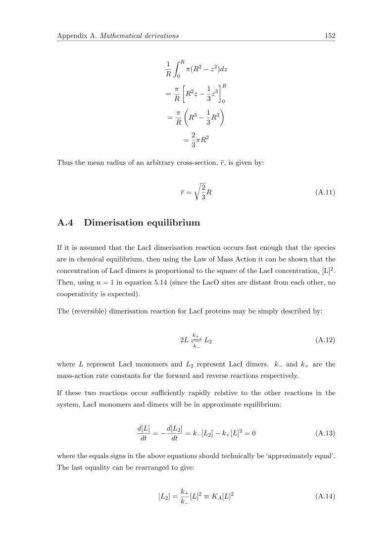
Appendix A. Mathematical derivations 152
1
R
∫ R
0π(R2 − z2)dz
=π
R
[R2z − 1
3z3]R0
=π
R
(R3 − 1
3R3
)=
2
3πR2
Thus the mean radius of an arbitrary cross-section, r, is given by:
r =
√2
3R (A.11)
A.4 Dimerisation equilibrium
If it is assumed that the LacI dimerisation reaction occurs fast enough that the species
are in chemical equilibrium, then using the Law of Mass Action it can be shown that the
concentration of LacI dimers is proportional to the square of the LacI concentration, [L]2.
Then, using n = 1 in equation 5.14 (since the LacO sites are distant from each other, no
cooperativity is expected).
The (reversible) dimerisation reaction for LacI proteins may be simply described by:
2Lk+−−⇀↽−−k−
L2 (A.12)
where L represent LacI monomers and L2 represent LacI dimers. k− and k+ are the
mass-action rate constants for the forward and reverse reactions respectively.
If these two reactions occur sufficiently rapidly relative to the other reactions in the
system, LacI monomers and dimers will be in approximate equilibrium:
d[L]
dt= −d[L2]
dt= k−[L2]− k+[L]2 = 0 (A.13)
where the equals signs in the above equations should technically be ‘approximately equal’.
The last equality can be rearranged to give:
[L2] =k+k−
[L]2 ≡ KA[L]2 (A.14)

Appendix A. Mathematical derivations 153
whereKA is the association constant of reaction A.12, defined as k+k−
. This is the expression
used in the main text in Chapter 5.2.4.
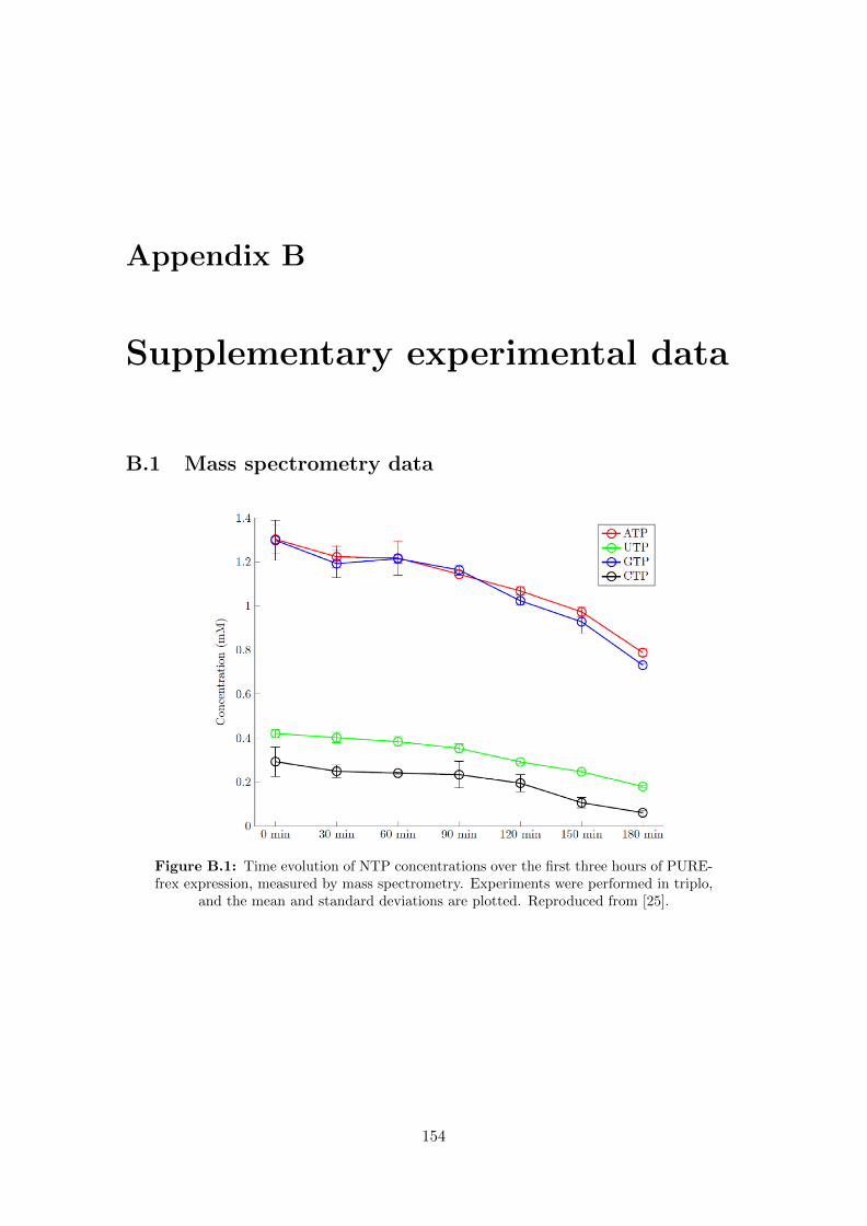
Appendix B
Supplementary experimental data
B.1 Mass spectrometry data
Figure B.1: Time evolution of NTP concentrations over the first three hours of PURE-frex expression, measured by mass spectrometry. Experiments were performed in triplo,
and the mean and standard deviations are plotted. Reproduced from [25].
154

Appendix B. Supplementary experimental data 155
Figure B.2: Time evolution of amino acid concentrations over the first 2.5 hours ofPUREfrex expression, measured by mass spectrometry. The anomalously low concen-tration of cysteine is considered an artificial experimental artefact, because it does notdetectably deplete over this time period, despite a comparable concentration of YFPbeing produced. According to the manufacturer, the concentration of all amino acids
should be (approximately) equal (Appendix C).

Appendix B. Supplementary experimental data 156
B.2 Time dependent deactivation fitting
(a)
(b)
Figure B.3: Fitting experimental data (solid lines) with De Mulder’s Genlink model ofPUREfrex expression (open circles) using (a) constant versus (b) translation-dependentribosome deactivation. The fitting of the plateau is seen to be superior in the translation-
dependent case. Reproduced from [20].
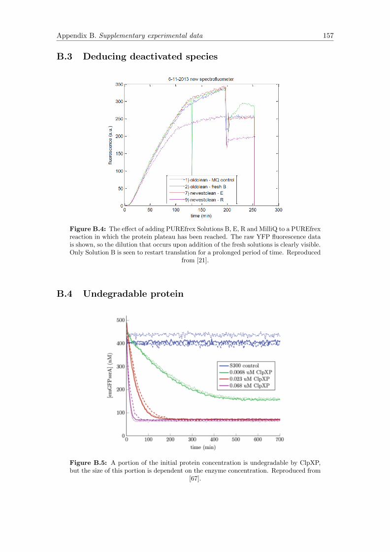
Appendix B. Supplementary experimental data 157
B.3 Deducing deactivated species
Figure B.4: The effect of adding PUREfrex Solutions B, E, R and MilliQ to a PUREfrexreaction in which the protein plateau has been reached. The raw YFP fluorescence datais shown, so the dilution that occurs upon addition of the fresh solutions is clearly visible.Only Solution B is seen to restart translation for a prolonged period of time. Reproduced
from [21].
B.4 Undegradable protein
Figure B.5: A portion of the initial protein concentration is undegradable by ClpXP,but the size of this portion is dependent on the enzyme concentration. Reproduced from
[67].
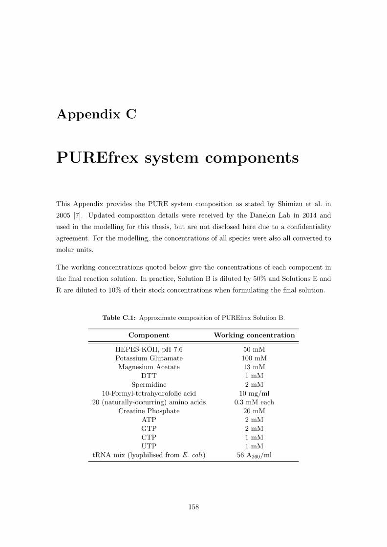
Appendix C
PUREfrex system components
This Appendix provides the PURE system composition as stated by Shimizu et al. in
2005 [7]. Updated composition details were received by the Danelon Lab in 2014 and
used in the modelling for this thesis, but are not disclosed here due to a confidentiality
agreement. For the modelling, the concentrations of all species were also all converted to
molar units.
The working concentrations quoted below give the concentrations of each component in
the final reaction solution. In practice, Solution B is diluted by 50% and Solutions E and
R are diluted to 10% of their stock concentrations when formulating the final solution.
Table C.1: Approximate composition of PUREfrex Solution B.
Component Working concentration
HEPES-KOH, pH 7.6 50 mMPotassium Glutamate 100 mMMagnesium Acetate 13 mM
DTT 1 mMSpermidine 2 mM
10-Formyl-tetrahydrofolic acid 10 mg/ml20 (naturally-occurring) amino acids 0.3 mM each
Creatine Phosphate 20 mMATP 2 mMGTP 2 mMCTP 1 mMUTP 1 mM
tRNA mix (lyophilised from E. coli) 56 A260/ml
158
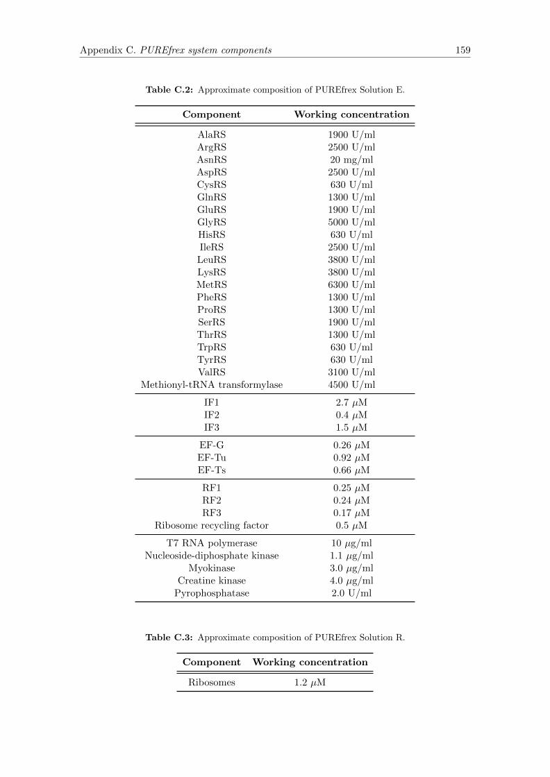
Appendix C. PUREfrex system components 159
Table C.2: Approximate composition of PUREfrex Solution E.
Component Working concentration
AlaRS 1900 U/mlArgRS 2500 U/mlAsnRS 20 mg/mlAspRS 2500 U/mlCysRS 630 U/mlGlnRS 1300 U/mlGluRS 1900 U/mlGlyRS 5000 U/mlHisRS 630 U/mlIleRS 2500 U/mlLeuRS 3800 U/mlLysRS 3800 U/mlMetRS 6300 U/mlPheRS 1300 U/mlProRS 1300 U/mlSerRS 1900 U/mlThrRS 1300 U/mlTrpRS 630 U/mlTyrRS 630 U/mlValRS 3100 U/ml
Methionyl-tRNA transformylase 4500 U/ml
IF1 2.7 µMIF2 0.4 µMIF3 1.5 µM
EF-G 0.26 µMEF-Tu 0.92 µMEF-Ts 0.66 µM
RF1 0.25 µMRF2 0.24 µMRF3 0.17 µM
Ribosome recycling factor 0.5 µM
T7 RNA polymerase 10 µg/mlNucleoside-diphosphate kinase 1.1 µg/ml
Myokinase 3.0 µg/mlCreatine kinase 4.0 µg/ml
Pyrophosphatase 2.0 U/ml
Table C.3: Approximate composition of PUREfrex Solution R.
Component Working concentration
Ribosomes 1.2 µM
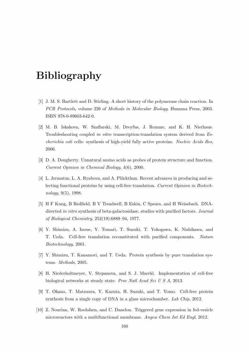
Bibliography
[1] J. M. S. Bartlett and D. Stirling. A short history of the polymerase chain reaction. In
PCR Protocols, volume 226 of Methods in Molecular Biology. Humana Press, 2003.
ISBN 978-0-89603-642-0.
[2] M. B. Iskakova, W. Szaflarski, M. Dreyfus, J. Remme, and K. H. Nierhaus.
Troubleshooting coupled in vitro transcription-translation system derived from Es-
cherichia coli cells: synthesis of high-yield fully active proteins. Nucleic Acids Res,
2006.
[3] D. A. Dougherty. Unnatural amino acids as probes of protein structure and function.
Current Opinion in Chemical Biology, 4(6), 2000.
[4] L. Jermutus, L. A. Ryabova, and A. Pluckthun. Recent advances in producing and se-
lecting functional proteins by using cell-free translation. Current Opinion in Biotech-
nology, 9(5), 1998.
[5] H F Kung, B Redfield, B V Treadwell, B Eskin, C Spears, and H Weissbach. DNA-
directed in vitro synthesis of beta-galactosidase. studies with purified factors. Journal
of Biological Chemistry, 252(19):6889–94, 1977.
[6] Y. Shimizu, A. Inoue, Y. Tomari, T. Suzuki, T. Yokogawa, K. Nishikawa, and
T. Ueda. Cell-free translation reconstituted with purified components. Nature
Biotechnology, 2001.
[7] Y. Shimizu, T. Kanamori, and T. Ueda. Protein synthesis by pure translation sys-
tems. Methods, 2005.
[8] H. Niederholtmeyer, V. Stepanova, and S. J. Maerkl. Implementation of cell-free
biological networks at steady state. Proc Natl Acad Sci U S A, 2013.
[9] T. Okano, T. Matsuura, Y. Kazuta, H. Suzuki, and T. Yomo. Cell-free protein
synthesis from a single copy of DNA in a glass microchamber. Lab Chip, 2012.
[10] Z. Nourian, W. Roelofsen, and C. Danelon. Triggered gene expression in fed-vesicle
microreactors with a multifunctional membrane. Angew Chem Int Ed Engl, 2012.
160

Bibliography 161
[11] Z. Nourian and C. Danelon. Linking genotype and phenotype in protein synthesizing
liposomes with external supply of resources. ACS Synth Biol, 2013.
[12] T. Stogbauer, L. Windhager, R. Zimmer, and J. O. Radler. Experiment and math-
ematical modeling of gene expression dynamics in a cell-free system. Integr Biol
(Camb), 2012.
[13] P. van Nies, Z. Nourian, M. Kok, R. van Wijk, J. Moeskops, I. Westerlaken, J. M.
Poolman, R. Eelkema, J. H. van Esch, Y. Kuruma, T. Ueda, and C. Danelon. Un-
biased tracking of the progression of mRNA and protein synthesis in bulk and in
liposome-confined reactions. Chembiochem, 2013.
[14] E. P. Solomon, Berg L. R., and Martin D. W. Biology. Cengage Learning, 7th edition,
2005.
[15] R. Phillips, J. Kondev, J. Theriot, and H. G. Garcia. Physical Biology of the Cell.
2nd edition.
[16] K. C. van Schie. Modelling gene expression in the PURE system, an in vitro protein
systhesis kit. Master Thesis, 2012.
[17] J. Marshall, R. Molloy, G. W. J. Moss, J. R. Howe, and T. E. Hughes. The jelly-
fish green fluorescent protein: A new tool for studying ion channel expression and
function. Neuron, 14(2):211 – 215, 1995.
[18] J. Ellenberg, J. Lippincott-Schwartz, and J. F. Presley. Dual-colour imaging with
GFP variants. Trends in Cell Biology, 1999.
[19] R. L. Strack and S. R. Jaffrey. New approaches for sensing metabolites and proteins
in live cells using RNA. Current Opinion in Chemical Biology, 2013.
[20] A. de Mulder. Modelling gene expression with CUDA and Genlink. Master Thesis,
2013.
[21] J. van der Wolf. The PURE system, ClpXP and MazF: experiments and modelling.
Post-thesis report, 2013.
[22] E. Gerritse. Modelling gene expression in bulk in the PURE system at different
temperatures. Bachelor thesis, 2014.
[23] Anonymous. Beating the edge effect. Laboratory News, 2011. Retrieved from http:
//www.labnews.co.uk/features/beating-the-edge-effect/ on 2014-09-09.
[24] Corning Incorporated. Corning Microplate Selection Guide for assays and drug dis-
covery. CLS-MP-014REV5, 2007.

Bibliography 162
[25] R. J. van Wijk. Towards a quantitative description of the PURE system dynamics.
Master Thesis, 2013.
[26] BMG Labtech. Clariostar Software User Manual. Version 5.01.
[27] P. van Nies, A. Soler Canton, Z. Nourian, and C. Danelon. Monitoring mRNA
and protein levels in bulk and in model vesicle-based artificial cells. Methods in
Enzymology, submitted.
[28] Nikon. NIS-Elements User Manual. Version 4.00.
[29] F. C. Rossetti, L. V. Depieri, and M. V. L. P. Bentley. Confocal Laser Scanning
Microscopy as a Tool for the Investigation of Skin Drug Delivery Systems and Diag-
nosis of Skin Disorders. Confocal Laser Microscopy - Principles and Applications in
Medicine, Biology, and the Food Sciences. Intechopen, 2013.
[30] Shinya Inoue. Foundations of confocal scanned imaging in light microscopy. In
James B. Pawley, editor, Handbook Of Biological Confocal Microscopy. Springer US,
2006.
[31] M. G. Gustafsson, L. Shao, P. M. Carlton, C. J. Wang, I. N. Golubovskaya, W. Z.
Cande, D. A. Agard, and J. W. Sedat. Three-dimensional resolution doubling in
wide-field fluorescence microscopy by structured illumination. Biophys J, 2008.
[32] Chroma Spectra Viewer. Accessed: 2014-09-09.
[33] A. D. Bantly, B. D. Gray, E. Breslin, E. G. Weinstein, K. A. Muirhead, B. M.
Ohlsson-Wilhelm, and J. S. Moore. CellVue Claret, a new far-red dye, facilitates
polychromatic assessment of immune cell proliferation. Informa Healthcare, 2007.
[34] A. B. Kudryavtsev, R. F. Jameson, and W. Linert. The Law of Mass Action. Springer
Science & Business Media, 2001.
[35] Eyal Karzbrun, Jonghyeon Shin, Roy H. Bar-Ziv, and Vincent Noireaux. Coarse-
grained dynamics of protein synthesis in a cell-free system. Physical Review Letters,
2011.
[36] A. Ujvari and C. T. Martin. Thermodynamic and kinetic measurements of promoter
binding by T7 RNA polymerase. Biochemistry, 1996.
[37] E. Sokolova, E. Spruijt, M. M. K. Hansen, E. Dubruc, J. Groen, V. Chokkalingam,
A. Piruska, H. A. Heus, and W. T. S. Huck. Enhanced transcription rates in
membrane-free protocells formed by coacervation of cell lysate. Proc Natl Acad Sci
U S A, 2013.
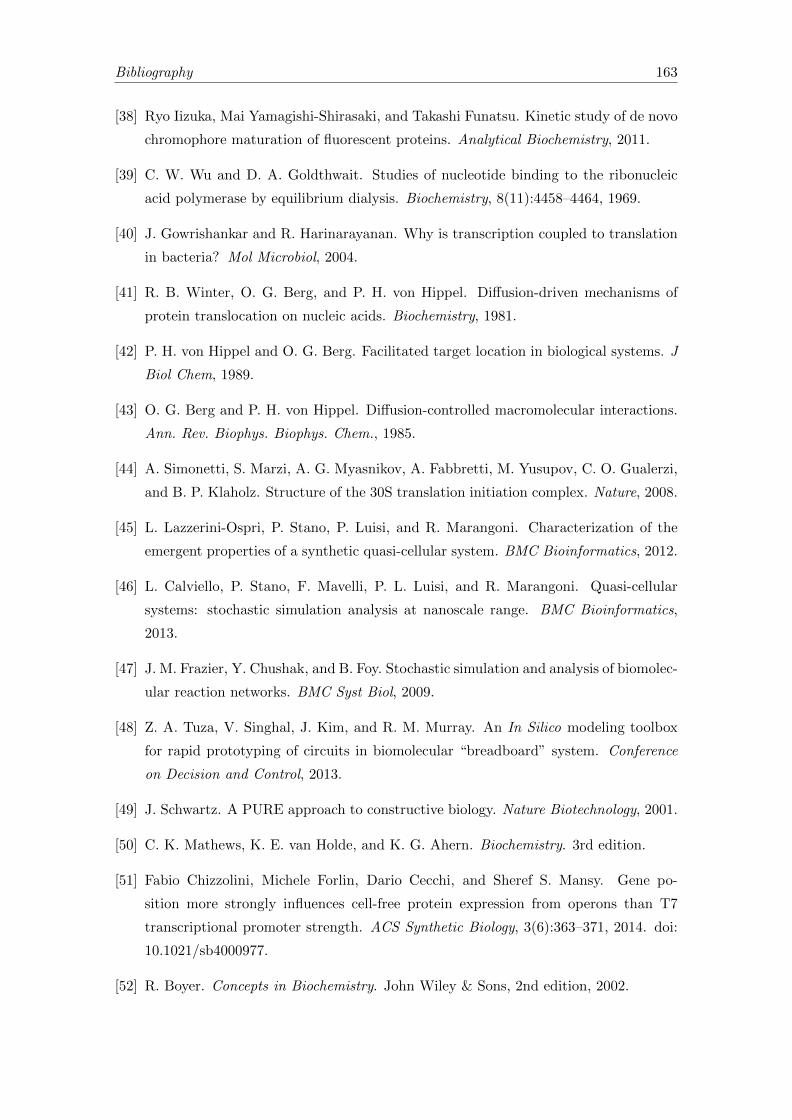
Bibliography 163
[38] Ryo Iizuka, Mai Yamagishi-Shirasaki, and Takashi Funatsu. Kinetic study of de novo
chromophore maturation of fluorescent proteins. Analytical Biochemistry, 2011.
[39] C. W. Wu and D. A. Goldthwait. Studies of nucleotide binding to the ribonucleic
acid polymerase by equilibrium dialysis. Biochemistry, 8(11):4458–4464, 1969.
[40] J. Gowrishankar and R. Harinarayanan. Why is transcription coupled to translation
in bacteria? Mol Microbiol, 2004.
[41] R. B. Winter, O. G. Berg, and P. H. von Hippel. Diffusion-driven mechanisms of
protein translocation on nucleic acids. Biochemistry, 1981.
[42] P. H. von Hippel and O. G. Berg. Facilitated target location in biological systems. J
Biol Chem, 1989.
[43] O. G. Berg and P. H. von Hippel. Diffusion-controlled macromolecular interactions.
Ann. Rev. Biophys. Biophys. Chem., 1985.
[44] A. Simonetti, S. Marzi, A. G. Myasnikov, A. Fabbretti, M. Yusupov, C. O. Gualerzi,
and B. P. Klaholz. Structure of the 30S translation initiation complex. Nature, 2008.
[45] L. Lazzerini-Ospri, P. Stano, P. Luisi, and R. Marangoni. Characterization of the
emergent properties of a synthetic quasi-cellular system. BMC Bioinformatics, 2012.
[46] L. Calviello, P. Stano, F. Mavelli, P. L. Luisi, and R. Marangoni. Quasi-cellular
systems: stochastic simulation analysis at nanoscale range. BMC Bioinformatics,
2013.
[47] J. M. Frazier, Y. Chushak, and B. Foy. Stochastic simulation and analysis of biomolec-
ular reaction networks. BMC Syst Biol, 2009.
[48] Z. A. Tuza, V. Singhal, J. Kim, and R. M. Murray. An In Silico modeling toolbox
for rapid prototyping of circuits in biomolecular “breadboard” system. Conference
on Decision and Control, 2013.
[49] J. Schwartz. A PURE approach to constructive biology. Nature Biotechnology, 2001.
[50] C. K. Mathews, K. E. van Holde, and K. G. Ahern. Biochemistry. 3rd edition.
[51] Fabio Chizzolini, Michele Forlin, Dario Cecchi, and Sheref S. Mansy. Gene po-
sition more strongly influences cell-free protein expression from operons than T7
transcriptional promoter strength. ACS Synthetic Biology, 3(6):363–371, 2014. doi:
10.1021/sb4000977.
[52] R. Boyer. Concepts in Biochemistry. John Wiley & Sons, 2nd edition, 2002.

Bibliography 164
[53] H. Bhaskaran, A. Rodriguez-Hernandez, and J. J. Perona. Kinetics of tRNA folding
monitored by aminoacylation. RNA, 2012.
[54] Johan Paulsson. Models of stochastic gene expression. Physics of Life Reviews, 2005.
[55] D. A. Potoyan and P. G. Wolynes. On the dephasing of genetic oscillators. Proc Natl
Acad Sci U S A, 2014.
[56] G. Karlebach and R. Shamir. Modelling and analysis of gene regulatory networks.
Nat Rev Mol Cell Biol, 2008.
[57] T. R. Maarleveld, B. G. Olivier, and F. J. Bruggeman. StochPy: a comprehensive,
user-friendly tool for simulating stochastic biological processes. PLoS One, 2013.
[58] D. T. Gillespie. Stochastic simulation of chemical kinetics. Annu Rev Phys Chem,
2007.
[59] P. L. Luisi, M. Allegretti, T. Pereira de Souza, F. Steiniger, A. Fahr, and P. Stano.
Spontaneous protein crowding in liposomes: a new vista for the origin of cellular
metabolism. Chembiochem, 2010.
[60] P. Siuti, S. T. Retterer, and M. J. Doktycz. Continuous protein production in
nanoporous, picolitre volume containers. Lab Chip, 2011.
[61] P. L. Luisi. The Emergence of Life. Cambridge University Press, 2006.
[62] E. M. Ozbudak, M. Thattai, I. Kurtser, A. D. Grossman, and A. van Oudenaarden.
Regulation of noise in the expression of a single gene. Nat Genet, 2002.
[63] K. F. Riley, M. P. Hobson, and S. J. Bence. Mathematical Methods for Physics and
Engineering. Cambridge University Press, 3rd edition, 2006.
[64] T. P. de Souza, P. Stano, F. Steiniger, E. D’Aguanno, E. Altamura, A. Fahr, and
P. L. Luisi. Encapsulation of ferritin, ribosomes, and ribo-peptidic complexes inside
liposomes: insights into the origin of metabolism. Orig Life Evol Biosph, 2012.
[65] J. Stricker, S. Cookson, M. R. Bennett, W. H. Mather, L. S. Tsimring, and J. Hasty.
A fast, robust and tunable synthetic gene oscillator. Nature, 2008.
[66] Arthur D. Riggs, Suzanne Bourgeois, and Melvin Cohn. The lac repressor-operator
interaction: III. Kinetic studies. Journal of Molecular Biology, 1970.
[67] J. van der Wolf. ClpXP-driven protein degradation and expression inhibition in the
PURE system. Master Thesis, 2013.
[68] A. Soler Canton. Controlled degradation of mRNA in the PURE system. Master
Thesis, 2013.
Bibliography 165
[69] B. Novak and J. J. Tyson. Design principles of biochemical oscillators. Nat Rev Mol
Cell Biol, 2008.
[70] E. Yeung, J. Kim, and R. M. Murray. Resource competition as a source of non-
minimum phase behavior in transcription-translation systems. Conference on Deci-
sion and Control, 2013.
[71] U. Vogel and K. F. Jensen. The RNA chain elongation rate in escherichia coli depends
on the growth rate. J. Bacteriol., 1994.
[72] R.Y. Young and H. Bremer. Polypeptide-chain-elongation rate in Escherichia coli
B/r as a function of growth rate. Biochem. J., 1976.
[73] J. R. Karr, J. C. Sanghvi, D. N. Macklin, M. V. Gutschow, J. M. Jacobs, Jr. Bolival,
B., N. Assad-Garcia, J. I. Glass, and M. W. Covert. A whole-cell computational
model predicts phenotype from genotype. Cell, 2012.
[74] G. L. Hersch, T. A. Baker, and R. T. Sauer. SspB delivery of substrates for ClpXP
proteolysis probed by the design of improved degradation tags. Proc Natl Acad Sci
U S A, 2004.
[75] A. N. Naganathan and V. Munoz. Scaling of folding times with protein size. J Am
Chem Soc, 127, 2005.
[76] William Mather, Matthew Bennett, Jeff Hasty, and Lev Tsimring. Delay-induced
degrade-and-fire oscillations in small genetic circuits. Physical Review Letters, 2009.
[77] G. Rodrigo, B. Kirov, S. Shen, and A. Jaramillo. Theoretical and experimental
analysis of the forced LacI-AraC oscillator with a minimal gene regulatory model.
Chaos, 2013.
[78] E. L. O’Brien, E. V. Itallie, and M. R. Bennett. Modeling synthetic gene oscillators.
Math Biosci, 2012.
[79] C. J. Wilson, P. Das, C. Clementi, K. S. Matthews, and P. Wittung-Stafshede. The
experimental folding landscape of monomeric lactose repressor, a large two-domain
protein, involves two kinetic intermediates. Proc Natl Acad Sci U S A, 2005.
[80] A. Szilagyi, J. Kardos, S. Osvath, L. Barna, and P. Zadovsky. Handbook of Neuro-
chemistry and Molecular Neurobiology. Springer Reference, 3rd edition, 2007.
[81] J. M. Vilar and L. Saiz. Reliable prediction of complex phenotypes from a modular
design in free energy space: an extensive exploration of the lac operon. ACS Synth
Biol, 2013.
[82] G. Weber. Energetics of Ligand Binding to Proteins. Academic Press Inc., 1975.

Bibliography 166
[83] Yannick Rondelez. Competition for catalytic resources alters biological network dy-
namics. Physical Review Letters, 2012.
[84] W. W. Wong, T. Y. Tsai, and J. C. Liao. Single-cell zeroth-order protein degradation
enhances the robustness of synthetic oscillator. Mol Syst Biol, 2007.
[85] B. van den Berg, R. J. Ellis, and C. M. Dobson. Effects of macromolecular crowding
on protein folding and aggregation. EMBO, 1999.
[86] S. M. Ross. Probability and Statistics for Engineers and Scientists. Academic Press,
4th edition, 2009.
[87] L. Lyons. A Practical Guide to Data Analysis for Physical Science Students. Cam-
bridge University Press, 1991.