Deterministic Global Optimization of Nonlinear Dynamic Systems

Youdong Lin and Mark A. Stadtherr∗

Department of Chemical and Biomolecular EngineeringUniversity of Notre Dame, Notre Dame, IN 46556, USA

(August 1, 2006)revised, December 1, 2006

∗Author to whom all correspondence should be addressed. E-mail: markst@nd.edu

Abstract

A new approach is described for the deterministic global optimization of dynamic systems, in-

cluding optimal control problems. The method is based on interval analysis and Taylor models and

employs a type of sequential approach. A key feature of the method is the use of a new validated

solver for parametric ODEs, which is used to produce guaranteed bounds on the solutions of dy-

namic systems with interval-valued parameters. This is combined with a new technique for domain

reduction based on the use of Taylor models in an efficient constraint propagation scheme. The re-

sult is that an ε-global optimum can be found with both mathematical and computational certainty.

Computational studies on benchmark problems are presented showing that this new approach pro-

vides significant improvements in computational efficiency, well over an order of magnitude in most

cases, relative to other recently described methods.

Keywords: Global optimization; Dynamic modeling; Interval analysis; Validated computing; Op-

timal control

Introduction

The dynamic behavior of many physical systems of practical interest can be modeled using

systems of ordinary differential equations (ODEs). Optimization problems involving these dynamic

models arise when optimal performance measures are sought for such systems. There are many

applications of dynamic optimization, including parameter estimation from time series data, de-

termination of optimal operating profiles for batch and semi-batch processes, optimal start-up,

shut-down, and switching of continuous system, etc.

To address this problem, one class of methods is based on discretization techniques to reduce

what is essentially an infinite-dimensional optimization problem to a finite-dimensional problem.

Two different discretization strategies are available: (a) the complete discretization or simulta-

neous approach,1,2 in which both state variables and control parameters are discretized, and (b)

the control parameterization or sequential approach,3,4 in which only the control parameters are

discretized. In this paper, only the control parameterization approach is considered. Since these

problems are often nonconvex and thus may exhibit multiple local solutions, the classical techniques

based on solving the necessary conditions for a local minimum may fail to determine the global

optimum. This is true even for a rather simple temperature control problem with a batch reactor.5

Therefore, there is a need to develop global optimization algorithms which can rigorously guarantee

optimal performance.

The deterministic global optimization of dynamic systems has been a topic of significant recent

interest. Esposito and Floudas6,7 used the αBB approach8,9 for addressing this problem. In

this method convex underestimating functions are used in connection with a branch-and-bound

framework. A theoretical guarantee of attaining an ε-global solution is offered as long as rigorous

underestimators are used, and this requires that sufficiently large values of α be used. However, the

determination of proper values of α depends on the Hessian of the function being underestimated,

1

and, when the sequential approach is used, this matrix is not available in explicit functional form.

Thus, Esposito and Floudas6,7 did not use rigorous values of α in their implementation of the

sequential approach, and so did not obtain a theoretical guarantee of global optimality. This issue is

discussed in more detail by Papamichail and Adjiman.10 Recently, alternative approaches have been

given by Chachuat and Latifi11 and by Papamichail and Adjiman10,12 that provide a theoretical

guarantee of ε-global optimality. However, this is achieved at a high computational cost. Singer

and Barton13 have recently described a branch-and-bound approach for determining an ε-global

optimum with significantly less computational effort. In this method, convex underestimators and

concave overestimators are used to construct two bounding initial value problems (IVPs), which are

then solved to obtain lower and upper bounds on the trajectories of the state variables.14 However,

as implemented,15 the bounding IVPs are solved using standard numerical methods that do not

provide guaranteed error estimates. Thus, strictly speaking, this approach cannot be regarded as

providing computationally guaranteed results.

We present here a new approach for the deterministic global optimization of dynamic systems.

This method is based on interval analysis and Taylor models and employs a type of sequential

approach. Instead of the usual branch-and-bound approach, we incorporate a new domain reduc-

tion technique, and thus use a type of branch-and-reduce strategy.16 A key feature of the method

is the use of a new validated solver17 for parametric ODEs, which is used to produce guaranteed

bounds on the solutions of dynamic systems with interval-valued parameters. The result is that

an ε-global optimum can be found with both mathematical and computational certainty. The

computational efficiency of this approach will be demonstrated through application to benchmark

problems, including optimal control problems. In the context of optimal control, a global mini-

mization algorithm based on different validated ODE solvers has recently been presented by Rauh

et al.18

2

The remainder of this paper is organized as follows. In the next section, we present the math-

ematical formulation of the problem to be solved. This is followed by a section that provides

background on interval analysis and Taylor models, a section in which we review the new validated

method17 for parametric ODEs, and a section in which we outline the algorithm for determin-

istic global optimization of dynamic systems. Finally, we present the results of some numerical

experiments that demonstrate the effectiveness of the approach presented.

Problem Statement

In this section we give the mathematical formulation of the nonlinear dynamic optimization

problem to be solved. Assume the system is described by the nonlinear ODE model x = f(x,θ).

Here x is the vector of state variables (length n) and θ is a vector of adjustable parameters (length

p), which may be a parameterization of a control profile θ(t). The model is given as an autonomous

system; a non-autonomous system can easily be converted into autonomous form by treating the

independent variable (t) as an additional state variable with derivative equal to 1. The objective

function φ is expressed in terms of the adjustable parameters and the values of the states at discrete

points tµ, µ = 0, 1, . . . , r. That is, φ = φ [xµ(θ),θ; µ = 0, 1, . . . , r], where xµ(θ) = x(tµ,θ). If an

integral appears in the objective function, it can be eliminated by introducing an appropriate

quadrature variable.

3

The optimization problem is then stated as

minθ,xµ

φ [xµ(θ),θ; µ = 0, 1, . . . , r] (1)

s.t. x = f(x,θ)

x0 = x0(θ)

t ∈ [t0, tr]

θ ∈ Θ.

Here Θ is an interval vector that provides upper and lower parameter bounds. We assume that f

is (k − 1)-times continuously differentiable with respect to the state variables x, and (q + 1)-times

continuously differentiable with respect to the parameters θ. We also assume that φ is (q+1)-times

continuously differentiable with respect to the parameters θ. Here k is the order of the truncation

error in the interval Taylor series (ITS) method to be used in the integration procedure, and q is the

order of the Taylor model to be used to represent parameter dependence. When a typical sequential

approach is used, an ODE solver is applied to the constraints with a given set of parameter values,

as determined by the optimization routine. This effectively eliminates xµ, µ = 0, 1, . . . , r, and leaves

a bound-constrained minimization in the adjustable parameters θ only.

A new method is described below for the deterministic global solution of Problem (1). This

method can also be easily extended to solve optimization problems with state path constraints

and more general equality or inequality constraints involving the parameters. This can be done by

adapting the constraint propagation procedure to handle the additional constraints.

4

Background

Interval analysis

A real interval X is defined as the set of real numbers lying between (and including) given upper

and lower bounds; that is,

X =[X,X

]={x ∈ R | X ≤ x ≤ X

}. (2)

Here an underline is used to indicate the lower bound of an interval and an overline is used to

indicate the upper bound. A real interval vector X = (X1, X2, · · · , Xn)T has n real interval

components and can be interpreted geometrically as an n-dimensional rectangle or box. Note that

in this context uppercase quantities are intervals, and lowercase quantities or uppercase quantities

with underline or overline are real numbers.

Basic arithmetic operations with intervals are defined by

X op Y = {x op y | x ∈ X, y ∈ Y } , (3)

where op ∈ {+,−,×,÷}. Interval versions of the elementary functions can be similarly defined.

It should be emphasized that, when machine computations with interval arithmetic operations

are done, as in the procedures outlined below, the endpoints of an interval are computed with a

directed (outward) rounding. That is, the lower endpoint is rounded down to the next machine-

representable number and the upper endpoint is rounded up to the next machine-representable

number. In this way, through the use of interval, as opposed to floating-point arithmetic, any

potential rounding error problems are avoided. Several good introductions to interval analysis,

as well as interval arithmetic and other aspects of computing with intervals, including their use

in global optimization, are available.19–22 Implementations of interval arithmetic and elementary

functions are also readily available, and recent compilers from Sun Microsystems directly support

interval arithmetic and an interval data type.

5

For an arbitrary function f(x), the interval extension, F (X) encloses all possible values of

f(x) for x ∈ X. That is, F (X) ⊇ {f(x) | x ∈ X} encloses the range of f(x) over X. It is

often computed by substituting the given interval X into the function f(x) and then evaluating

the function using interval arithmetic. This so-called “natural” interval extension is sometimes

wider than the actual range of function values, though it always includes the actual range. For

example, the natural interval extension of f(x) = x/(x−1) over the interval X = [2, 3] is F ([2, 3]) =

[2, 3]/([2, 3]−1) = [2, 3]/[1, 2] = [1, 3], while the true function range over this interval is [1.5, 2]. This

overestimation of the function range is due to the “dependency” problem, which may arise when a

variable occurs more than once in a function expression. While a variable may take on any value

within its interval, it must take on the same value each time it occurs in an expression. However,

this type of dependency is not recognized when the natural interval extension is computed. In

effect, when the natural interval extension is used, the range computed for the function is the range

that would occur if each instance of a particular variable was allowed to take on a different value

in its interval range. For the case in which f(x) is a single-use expression, that is, an expression in

which each variable occurs only once, natural interval arithmetic will always yield the true function

range. For example, rearrangement of the function expression used above gives f(x) = x/(x− 1) =

1 + 1/(x − 1), and now F ([2, 3]) = 1 + 1/([2, 3] − 1) = 1 + 1/[1, 2] = 1 + [0.5, 1] = [1.5, 2], the true

range.

In some situations, dependency issues can be avoided through the use of the dependent sub-

traction operation (also known as the cancellation operation). Assume that there is an interval

S that depends additively on the interval A. The dependent subtraction operation is defined by

SA = [S−A,S−A]. For example, let A = [1, 2], B = [2, 3], C = [3, 4] and S = A+B+C = [6, 9].

Say that only S is stored and that later it is desired to compute A + B by subtracting C from S.

Using the standard subtraction operation yields S −C = [6, 9] − [3, 4] = [2, 6], which overestimates

6

the true A + B. Using the dependent subtraction operation, which is allowable since S depends

additively on C, yields S C = [6, 9] [3, 4] = [3, 5], which is the true A + B. For more gen-

eral situations, there are a variety of other approaches that can be used to try to tighten interval

extensions,19–22 including the use of Taylor models, as described in the next subsection.

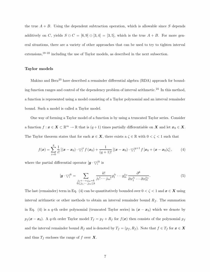
Taylor models

Makino and Berz23 have described a remainder differential algebra (RDA) approach for bound-

ing function ranges and control of the dependency problem of interval arithmetic.24 In this method,

a function is represented using a model consisting of a Taylor polynomial and an interval remainder

bound. Such a model is called a Taylor model.

One way of forming a Taylor model of a function is by using a truncated Taylor series. Consider

a function f : x ∈ X ⊂ Rm → R that is (q +1) times partially differentiable on X and let x0 ∈ X.

The Taylor theorem states that for each x ∈ X, there exists a ζ ∈ R with 0 < ζ < 1 such that

f(x) =

q∑

i=0

1

i![(x − x0) · 5]i f (x0) +

1

(q + 1)![(x − x0) · 5]q+1 f [x0 + (x − x0)ζ] , (4)

where the partial differential operator [g · 5]k is

[g · 5]k =∑

j1+···+jm=k0≤j1,··· ,jm≤k

k!

j1! · · · jm!gj11 · · · gjm

m

∂k

∂xj11 · · · ∂xjm

m

. (5)

The last (remainder) term in Eq. (4) can be quantitatively bounded over 0 < ζ < 1 and x ∈ X using

interval arithmetic or other methods to obtain an interval remainder bound Rf . The summation

in Eq. (4) is a q-th order polynomial (truncated Taylor series) in (x − x0) which we denote by

pf (x − x0). A q-th order Taylor model Tf = pf + Rf for f(x) then consists of the polynomial pf

and the interval remainder bound Rf and is denoted by Tf = (pf , Rf ). Note that f ∈ Tf for x ∈ X

and thus Tf encloses the range of f over X.

7

Taylor models of functions can also be formed by performing Taylor model operations. Arith-

metic operations with Taylor models can be done using the remainder differential algebra (RDA)

described by Makino and Berz.23–25 Let Tf and Tg be the Taylor models of the functions f(x) and

g(x), respectively, over the interval x ∈ X. For f ± g,

f ± g ∈ Tf ± Tg = (pf , Rf ) ± (pg, Rg) = (pf ± pg, Rf ± Rg). (6)

Thus a Taylor model of f ± g is given by

Tf±g = (pf±g, Rf±g) = (pf ± pg, Rf ± Rg). (7)

For the product f × g,

f × g ∈ (pf , Rf ) × (pg, Rg) ⊆ pf × pg + pf × Rg + pg × Rf + Rf × Rg. (8)

Note that pf × pg is a polynomial of order 2q. Since a q-th order polynomial is sought for the

Taylor model of f × g, this term is split pf × pg = pf×g + pe. Here the polynomial pf×g contains

all terms of order q or less, and pe contains the higher order terms. A q-th order Taylor model for

the product f × g can then be given by Tf×g = (pf×g, Rf×g), with

Rf×g = B(pe) + B(pf ) × Rg + B(pg) × Rf + Rf × Rg. (9)

Here B(p) = P (X − x0) denotes an interval bound on the polynomial p(x − x0) over x ∈ X.

Similarly, an interval bound on an overall Taylor model T = (p,R) will be denoted by B(T ), and is

computed by obtaining B(p) and adding it to the remainder bound R; that is, B(T ) = B(p) + R.

The method we use to obtain the polynomial bounds is described below. In storing and operating

on a Taylor model, only the coefficients of the polynomial part p are used, and these are point

valued. However, when these coefficients are computed in floating point arithmetic, numerical

errors may occur and they must be bounded. To do this in our current implementation of Taylor

model arithmetic, we have used the “tallying variable” approach, as described by Makino and

8

Berz.25 This approach has been analyzed in detail by Revol et al.26 This results in an error bound

on the floating point calculation of the coefficients in p being added to the interval remainder bound

R.

Taylor models for the reciprocal operation, as well as the intrinsic functions (exponential,

logarithm, sine, etc.) can also be obtained.23,25,27 Using these, together with the basic arith-

metic operations defined above, it is possible to start with simple functions such as the constant

function f(x) = k, for which Tf = (k, [0, 0]), and the identity function f(xi) = xi, for which

Tf = (xi0 + (xi − xi0), [0, 0]), and then to compute Taylor models for very complicated functions.

Altogether, it is possible to compute a Taylor model for any function that can be represented in a

computer environment by simple operator overloading through RDA operations. It has been shown

that, compared to other rigorous bounding methods, the Taylor model often yields sharper bounds

for modest to complicated functional dependencies.23,24,28 A discussion of the uses and limitations

of Taylor models has been given by Neumaier.28

The range bounding of the interval polynomials B(p) = P (X−x0) is an important issue, which

directly affects the performance of Taylor model methods. Unfortunately, exact range bounding of

an interval polynomial is NP hard, and direct evaluation using interval arithmetic is very inefficient,

often yielding only loose bounds. Thus, various bounding schemes28,29 have been used, mostly

focused on exact bounding of the dominant parts of P , i.e., the first- and second-order terms.

However, exact bounding of a general interval quadratic is also computationally expensive (in

the worst case, exponential in the number of variables m). Thus, we have adopted here a very

simple compromise approach, in which only the first-order and the diagonal second-order terms are

considered for exact bounding, and other terms are evaluated directly. That is,

B(p) =

m∑

i=1

[ai (Xi − xi0)

2 + bi(Xi − xi0)]

+ Q, (10)

where Q is the interval bound of all other terms, and is obtained by direct evaluation with interval

9

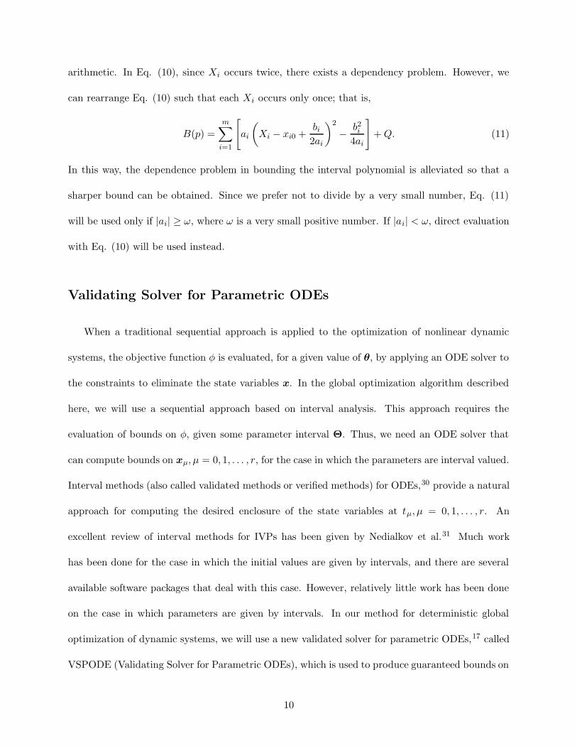
arithmetic. In Eq. (10), since Xi occurs twice, there exists a dependency problem. However, we

can rearrange Eq. (10) such that each Xi occurs only once; that is,

B(p) =m∑

i=1

[ai

(Xi − xi0 +

bi

2ai

)2

− b2i

4ai

]+ Q. (11)

In this way, the dependence problem in bounding the interval polynomial is alleviated so that a

sharper bound can be obtained. Since we prefer not to divide by a very small number, Eq. (11)

will be used only if |ai| ≥ ω, where ω is a very small positive number. If |ai| < ω, direct evaluation

with Eq. (10) will be used instead.

Validating Solver for Parametric ODEs

When a traditional sequential approach is applied to the optimization of nonlinear dynamic

systems, the objective function φ is evaluated, for a given value of θ, by applying an ODE solver to

the constraints to eliminate the state variables x. In the global optimization algorithm described

here, we will use a sequential approach based on interval analysis. This approach requires the

evaluation of bounds on φ, given some parameter interval Θ. Thus, we need an ODE solver that

can compute bounds on xµ, µ = 0, 1, . . . , r, for the case in which the parameters are interval valued.

Interval methods (also called validated methods or verified methods) for ODEs,30 provide a natural

approach for computing the desired enclosure of the state variables at tµ, µ = 0, 1, . . . , r. An

excellent review of interval methods for IVPs has been given by Nedialkov et al.31 Much work

has been done for the case in which the initial values are given by intervals, and there are several

available software packages that deal with this case. However, relatively little work has been done

on the case in which parameters are given by intervals. In our method for deterministic global

optimization of dynamic systems, we will use a new validated solver for parametric ODEs,17 called

VSPODE (Validating Solver for Parametric ODEs), which is used to produce guaranteed bounds on

10

the solutions of dynamic systems with interval-valued initial states and parameters. In this section,

we review the key ideas behind the new method used in VSPODE, and outline the procedures used.

Additional details are given by Lin and Stadtherr.17

Traditional interval methods usually consist of two processes applied at each integration step.31

In the first process, existence and uniqueness of the solution are proved using the Picard-Lindelof

operator and the Banach fixed point theorem,32 and a rough enclosure of the solution is computed.

In the second process, a tighter enclosure of the solution is computed. In general, both processes

are realized by applying interval Taylor series (ITS) expansions with respect to time, and using

automatic differentiation to obtain the Taylor coefficients. A major difficulty in interval methods is

the overestimation of bounds caused by the dependency problem of interval arithmetic and by the

wrapping effect.30 The accumulation of overestimations at successive time steps may ultimately

lead to an explosion of enclosure sizes, causing the integration procedure to abort. Several schemes

for reducing the overestimation of bounds have been proposed for the case of interval-valued initial

states. For example, Lohner’s AWA package employs a QR-factorization method which features

efficient coordinate transformations to tackle the wrapping effect.33 Nedialkov’s VNODE package

employs QR together with an interval Hermite-Obreschkoff method,34,35 which can be viewed as

a type of generalized Taylor method, and improves on AWA. Janssen et al.36 have introduced a

constraint satisfaction approach to these problems, which enhances traditional interval methods

with a pruning step based on a global relaxation of the ODEs. Another approach for addressing

the dependency problem and the wrapping effect has been described by Berz and Makino37 and

implemented in the beam dynamics package COSY INFINITY. This scheme is based on expressing

the dependence on initial values and time using a Taylor model. Neher et al.38 have recently de-

scribed this Taylor model approach in some detail and compared it to traditional interval methods.

Taylor models are also used in VSPODE, though they are determined and used in a different way,

11

and a new type of Taylor model, involving a parallelepiped remainder bound, is introduced.17

Consider the parametric ODE system occurring in the constraints of the optimization problem:

x = f(x,θ), x0 ∈ X0, θ ∈ Θ, (12)

where t ∈ [t0, tr] for some tr > t0. The interval vectors X0 = X0(Θ) and Θ represent enclosures

of initial values and parameters, respectively. It is desired to determine a validated enclosure

of all possible solutions to this initial value problem. We denote by x(t; tj ,Xj,Θ) the set of

solutions x(t; tj ,Xj ,Θ) = {x(t; tj ,xj,θ) | xj ∈ Xj ,θ ∈ Θ} , where x(t; tj ,xj ,θ) denotes a solution

of x = f(x,θ) for the initial condition x = xj at tj. We will outline a method for determining

enclosures Xj of the state variables at each time step j = 1, . . . , r, such that x(tj ; t0,X0,Θ) ⊆ Xj .

Assume that at tj we have an enclosure X j of x(tj; t0,X0,Θ), and that we want to carry out an

integration step to compute the next enclosure X j+1. Then, in the first phase of the method, the

goal is to find a step size hj = tj+1 − tj > 0 and an a prior enclosure (coarse enclosure) Xj of the

solution such that a unique solution x(t; tj ,xj,θ) ∈ Xj is guaranteed to exist for all t ∈ [tj , tj+1],

all xj ∈ Xj, and all θ ∈ Θ. We apply the traditional interval method, with high order enclosure,

to the parametric ODEs by using an interval Taylor series (ITS) with respect to time. That is, we

determine hj and Xj such that for Xj ⊆ X0

j ,

Xj =

k−1∑

i=0

[0, hj ]iF [i](Xj ,Θ) + [0, hj ]

kF [k](X0

j ,Θ) ⊆ X0

j . (13)

Here X0

j is an initial estimate of Xj, k denotes the order of the Taylor expansion, and the coefficients

F [i] are interval extensions of the Taylor coefficients f [i] of x(t) with respect to time, which can be

12

obtained recursively in terms of x(t) = f(x,θ) by

f [0] = x

f [1] = f(x,θ) (14)

f [i] =1

i

(∂f [i−1]

∂xf

)(x,θ), i ≥ 2.

Satisfaction of Eq. (13) demonstrates that there exists a unique solution x(t; tj ,xj,θ) ∈ Xj for all

t ∈ [tj , tj+1], all xj ∈ Xj, and all θ ∈ Θ.39 X0

j is initialized and hj is iteratively reduced, if needed

to satisfy Eq. (13), using the method described by Nedialkov et al.35

In the second phase of the method, we compute a tighter enclosure X j+1 ⊆ Xj , such that

x(tj+1; t0,X0,Θ) ⊆ Xj+1. This will be done by using an ITS approach to compute a Taylor

model T xj+1 of xj+1 in terms of the parameter vector θ, and then obtaining the enclosure X j+1 =

B(T xj+1) by bounding T xj+1 over θ ∈ Θ. For the Taylor model computations, we begin by

representing the parameters by the Taylor model T θ, with components

Tθi= (m(Θi) + (θi − m(Θi)), [0, 0]), i = 1, · · · , p, (15)

where m(Θi) indicates the midpoint of Θi. To determine enclosures of the interval Taylor series

coefficients f [i](xj,θ) a novel approach combining RDA operations with the mean value theorem

is used to obtain the Taylor models Tf [i]. Now using an interval Taylor series for xj+1 with

coefficients given by Tf [i] , one can obtain a result for T xj+1 in terms of the parameters. In order

to address the wrapping effect,30 results are propagated from one time step to the next using a

new type of Taylor model, in which the remainder bound is not an interval, but a parallelepiped.

That is, the remainder bound is a set of the form P = {Av | v ∈ V }, where A ∈ Rn×n is a real

and regular matrix. If A is orthogonal, as from a QR-factorization, then P can be interpreted as

a rotated n-dimensional rectangle. Complete details of the computation of T xj+1 are given by Lin

and Stadtherr.17

13

The approach outlined above, as implemented in VSPODE, has been tested by Lin and Stadt-

herr,17 who compared its performance with results obtained using the popular VNODE package35

(in using VNODE, interval-valued parameters are treated as additional state variables with interval-

valued initial states). For the test problems used, VSPODE provided tighter enclosures on the state

variables than VNODE, and required significantly less computation time.

Deterministic Global Optimization Method

In this section, we present a new method for the deterministic global optimization of dynamic

systems. This a generalization of the approach used by Lin and Stadtherr40 for the special case of

parameter estimation, in which the objective is a sum of squares function. As noted above, when a

sequential approach is used, the state variables are effectively eliminated using the ODE constraints,

in this case by employing VSPODE, leaving a bound-constrained minimization of φ(θ) with respect

to the adjustable parameters (decision variables) θ. The new approach can be thought of as a type

of branch-and-bound method, with a constraint propagation procedure used for domain reduction.

Therefore, it can also be viewed as a branch-and-reduce algorithm.16 The basic idea is that only

those parts of the decision variable space Θ that satisfy the constraint c(θ) = φ(θ)− φ ≤ 0, where

φ is a known upper bound on the global minimum, needs to be retained. We now describe a

constraint propagation procedure, based on the use of Taylor models, that exploits this constraint

information for domain reduction.

Constraint propagation on Taylor models

Partial information expressed by a constraint can be used to eliminate incompatible values from

the domain of its variables. This domain reduction can then be propagated to all constraints on

that variable, where it may be used to further reduce the domains of other variables. This process

14

is known as constraint propagation. In this subsection, we show how to apply such a constraint

propagation procedure using Taylor models.

Let Tc be the Taylor model of the function c(x) over the interval x ∈ X, and say the constraint

c(x) ≤ 0 needs to be satisfied. In the constraint propagation procedure (CPP) described here,

B(Tc) is determined and then there are three possible outcomes: 1. If B(Tc) > 0, then no x ∈ X

will ever satisfy the constraint; thus, the CPP can be stopped and X discarded. 2. If B(Tc) ≤ 0,

then every x ∈ X will always satisfy the constraint; thus X cannot be reduced and the CPP

can be stopped. 3. If neither of previous two cases occur, then part of the interval X may be

eliminated; thus the CPP continues as described below, using an approach based on the range

bounding strategy for Taylor models described above.

For some component i of x, let ai and bi be the polynomial coefficients of the terms (xi − xi0)2

and (xi − xi0) of Tc, respectively. Note that xi0 ∈ Xi and is usually the midpoint xi0 = m(Xi); the

value of xi0 will not change during the CPP. For |ai| ≥ ω, the bounds on Tc can be expressed using

Eq. (11) as

B(Tc) = ai

(Xi − xi0 +

bi

2ai

)2

− b2i

4ai+ Si, (16)

where

Si =m∑

j=1j 6=i

[aj

(Xj − xj0 +

bj

2aj

)2

−b2j

4aj

]+ Q. (17)

We can reduce the computational effort to obtain Si by recognizing that this quantity is just B(Tc)

less the i-th term in the summation, and B(Tc) was already computed earlier in the CPP. Thus,

for each i, Si can be determined by dependent subtraction (see above) using

Si = B(Tc) [ai

(Xi − xi0 +

bi

2ai

)2

− b2i

4ai

]. (18)

Now define the intervals Ui = Xi − xi0 + bi

2aiand Vi =

b2i4ai

− Si, so that B(Tc) = aiU2i − Vi. The

goal is to identify and retain only the part of Xi that contains values of xi for which it is possible

15

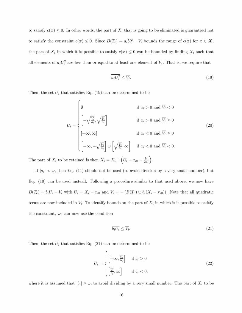
to satisfy c(x) ≤ 0. In other words, the part of Xi that is going to be eliminated is guaranteed not

to satisfy the constraint c(x) ≤ 0. Since B(Tc) = aiU2i − Vi bounds the range of c(x) for x ∈ X,

the part of Xi in which it is possible to satisfy c(x) ≤ 0 can be bounded by finding Xi such that

all elements of aiU2i are less than or equal to at least one element of Vi. That is, we require that

aiU2i ≤ Vi. (19)

Then, the set Ui that satisfies Eq. (19) can be determined to be

Ui =

∅ if ai > 0 and Vi < 0

[−√

Vi

ai,√

Vi

ai

]if ai > 0 and Vi ≥ 0

[−∞,∞] if ai < 0 and Vi ≥ 0

[−∞,−

√Vi

ai

]∪[√

Vi

ai,∞]

if ai < 0 and Vi < 0.

(20)

The part of Xi to be retained is then Xi = Xi ∩(Ui + xi0 − bi

2ai

).

If |ai| < ω, then Eq. (11) should not be used (to avoid division by a very small number), but

Eq. (10) can be used instead. Following a procedure similar to that used above, we now have

B(Tc) = biUi − Vi with Ui = Xi − xi0 and Vi = − (B(Tc) bi(Xi − xi0)). Note that all quadratic

terms are now included in Vi. To identify bounds on the part of Xi in which is it possible to satisfy

the constraint, we can now use the condition

biUi ≤ Vi. (21)

Then, the set Ui that satisfies Eq. (21) can be determined to be

Ui =

[−∞, Vi

bi

]if bi > 0

[Vi

bi,∞]

if bi < 0,

(22)

where it is assumed that |bi| ≥ ω, to avoid dividing by a very small number. The part of Xi to be

16

retained is then Xi = Xi ∩ (Ui + xi0). If both |ai| and |bi| are less than ω, then no CPP will be

applied on Xi.

The overall CPP is implemented by beginning with i = 1 and proceeding component by com-

ponent. If, for any i, the result Xi = ∅ is obtained, then no x ∈ X can satisfy the constraint; thus,

X can be discarded and the CPP stopped. Otherwise the CPP proceeds until all components of X

have been updated. Note that, in principle, each time an improved (smaller) Xi is found, it could

be used in computing Si for subsequent components of X . However, this requires recomputing the

bound B(Tc), which, for the function c(x) that is of interest here, is expensive. Thus, the CPP

for each component is done using the bounds B(Tc) computed from the original X. If, after each

component is processed, X has been sufficiently reduced (by more than ω1 = 10% by volume), then

a new bound B(Tc) is obtained, now over the smaller X, and a new CPP is started. Otherwise,

the CPP terminates.

Global optimization algorithm

As with any type of procedure incorporating branch-and-bound, an important issue is how to

initialize φ, the upper bound on the global minimum. There are many ways in which this can be

done, and clearly, it is desirable to find a φ that is as small as possible (i.e., the tightest possible

upper bound). To initialize φ, we run p2 local minimizations (p is the number of adjustable

parameters) using a local optimization routine from randomly chosen starting points, and then

choose the smallest value of φ found to be the initial φ. For this purpose, we use the bound-

constrained quasi-Newton method L-BFGS-B41 as the local optimization routine, and DDASSL42

as the integration routine. Additional initialization steps are to set either a relative convergence

tolerance εrel or an absolute convergence tolerance εabs, and initialize a work list L. The work

list (stack) L will contain a sequence of subintervals (boxes) that need to be tested and initially

17

L = {Θ}, the entire parameter (decision variable) space.

The core steps in the iterative process involve the testing of boxes in the work list. This is

an objective range test combined with domain reduction done using the CPP described above.

Beginning with k = 0, at the k-th iteration a box is removed from the front of L and is designated

as the current subinterval Θ(k). The Taylor model Tφkof the objective function φ over Θ(k) is

computed. To do this, Taylor models of xµ, the state variables at times tµ, µ = 1, . . . , r, in terms

of θ are determined using VSPODE, as described above. Note that Tφkthen consists of a q-th

order polynomial in the decision variables θ, plus a remainder bound. The part of Θ(k) that can

contain the global minimum must satisfy the constraint c(θ) = φ(θ) − φ ≤ 0 Thus the constraint

propagation procedure (CPP) described above is now applied using this constraint. Recall that

there are three possible outcomes in the CPP:

1. Testing for the first possible outcome, B(Tc) > 0, amounts to checking if the lower bound

of Tφk, B(Tφk

), is greater than φ. If so, then Θ(k) can be discarded because it cannot contain the

global minimum and need not be further tested.

2. Testing for the second possible outcome, B(Tc) ≤ 0, amounts to checking if the upper bound

of Tφk, B(Tφk

), is less than φ. If so, then all points in Θ(k) satisfy the constraint and the CPP can

be stopped since no reduction in Θ(k) can be achieved. This also indicates, with certainty, that

there is a point in Θ(k) that can be used to update φ. Thus, if B(Tφk) < φ, a local optimization

routine, starting at some point in Θ(k), is used to find a local minimum, which then provides an

updated (smaller) φ, that is, a better upper bound on the global minimum. In our implementation,

the midpoint of Θ(k) is used as the starting point for the local optimization. A new CPP is then

started on Θ(k) using the updated value of φ.

3. If neither of the previous two outcomes occurs, then the full CPP described above is applied

to reduce Θ(k). Note that if Θ(k) is sufficiently reduced (by more than ω1 = 10% by volume) in

18

comparison to its volume at the beginning of CPP, then new bounds B(Tφk) are obtained, now

over the smaller Θ(k), and a new CPP is started.

After the CPP terminates, a convergence test is performed. If (φ − B(Tφk))/|φ| ≤ εrel, or

(φ − B(Tφk)) ≤ εabs, then Θ(k) need not be further tested and can be discarded. Otherwise, we

will check to what extent Θ(k) has been reduced compared to its volume at the beginning of the

objective range test. If the subinterval has been reduced by more than ω2 = 70% by volume, it will

be added to the front of the sequence L of boxes to be tested. Otherwise, it will be bisected, and

the resulting two subintervals added to the front of L. Various strategies can be used to select the

component to be bisected. For the problems solved here, the component with the largest relative

width was selected for bisection. The relative width of a parameter component Θ(k)i is defined as

(Θ

(k)i − Θ

(k)i

)/max{| Θ

(k)i |, | Θ

(k)i |, 1}. The volume reduction targets ω1 and ω2 can be adjusted

as needed to tune the algorithm; the default values given above were used in the computational

studies described below. At the end of this testing process, k is incremented, a box is removed from

the front of L, and the testing process is begun again. At termination, L will become empty, and

φ is the ε-global minimum.

The method described above is an ε-global algorithm. It is also possible to incorporate interval-

Newton steps in the method, and to thus make it an exact algorithm. This requires the application

of VSPODE on the first- and second-order sensitivity equations. An exact algorithm using interval-

Newton steps has been implemented by Lin and Stadtherr40 for the special case of parameter

estimation problems, but has not yet been fully implemented for the more general case described

here.

19

Computational Studies

In this section, three example problems are presented to illustrate the theoretical and compu-

tational aspects of the proposed approach. All example problems were solved on an Intel Pentium

4 3.2GHz machine running Red Hat Linux. The VSPODE package,17 with a k = 17 order interval

Taylor series, q = 3 order Taylor model, and QR approach for wrapping, was used to integrate

the dynamic systems in each problem. Using a smaller ITS order k will result in the need for

smaller step sizes in the integration and so will tend to increase computation time. Using a larger

Taylor model order q will result in somewhat tighter bounds on the states, though at the expense

of additional complexity in the Taylor model computations. The algorithm was implemented in

C++.

Illustrative example

This problem has been used by several previous authors as an illustrative example. It involves

the optimization of a simple dynamic system, with one decision variable. The problem is formulated

as:

minθ

φ = −x2(tf ) (23)

s.t. x = −x2 + θ

x0 = 9

t ∈ [t0, tf ] = [0, 1]

θ ∈ [−5, 5].

It has been shown that Problem (23) has two local minima, one at each bound of the parameter

domain.11,12

We will illustrate here the optimization procedure described above by solving this problem to

20

an absolute tolerance of εabs = 10−3. First, the upper bound φ on the global minimum is initialized

using local optimization. This results in finding the local solution θ = −5 with objective value

φ = −8.23262154. The work list is initialized to L = {[−5, 5]}.

The main iteration is now begun with k = 0 (in this section k is an iteration counter and does

not refer to the order of the interval Taylor series used), and Θ(0) = [−5, 5] is removed from the

work list. VSPODE is now applied and a Taylor model Tφ0 of the objective function over Θ(0) is

obtained, with the result

Tφ0 = (−1.4347 − 0.6394(θ − 0) − 0.0865(θ − 0)2

+ 0.0167(θ − 0)3, [−9.212744, 9.212744]).

The bounds B(Tφ0) = [−18.098954, 11.053372] are now computed and the CPP is performed.

The CPP results in no reduction of the current interval; thus it is bisected and the resulting two

subintervals [−5, 0], and [0, 5] are added to the work sequence, giving L = {[−5, 0], [0, 5]}.

For the next iteration, k = 1 and Θ(1) = [−5, 0] is removed from the front of L. VSPODE is

applied and a Taylor model Tφ1 of the objective function over Θ(1) is obtained, resulting in

Tφ1 = (−0.2969 + 0.3949(θ + 2.5) − 0.4569(θ + 2.5)2

+ 0.1223(θ + 2.5)3, [−2.205915, 2.205915]).

The bounds are computed as B(Tφ1) = [−8.256285, 3.905142] and the CPP is applied. Applying

the CPP reduces the current subinterval to Θ(1) = [−5,−4.9911] and gives B(Tφ1) = −8.256285.

This does not satisfy the convergence test, but the volume of Θ(1) has been reduced by more

than 70%. Thus, the reduced subinterval is added to the front of the work array, giving L =

{[−5, 4.9911], [0, 5]}.

Next, with k = 2 and Θ(2) = [−5,−4.9911], the Taylor model of the objective computed using

21

VSPODE is

Tφ2 = (−8.18836 + 9.9814(θ + 4.99555) − 6.0120(θ + 4.99555)2

+ 2.7786(θ + 4.99555)3 , [−0.000001, 0.000001]),

and B(Tφ2) = [−8.232622,−8.144335]. After the CPP, the subinterval has been reduced to

[−5,−4.9999] and B(Tφ2) = −8.232622. Since B(Tφ2) satisfies the convergence condition, this

subinterval needs no further testing and can be discarded. Now L = {[0, 5]}.

Next, with k = 3 and Θ(3) = {[0, 5]}, the Taylor model of the objective function is

Tφ3 = (−2.8176 − 0.8901(θ − 2.5) − 0.0223(θ − 2.5)2

+ 0.0035(θ − 2.5)3, [−0.066276, 0.066276]),

and B(Tφ3) = [−5.302934,−0.610588]. Now in the CPP it is seen that B(Tφ3) > φ, so this

subinterval can be discarded. Now L = ∅, indicating termination. Thus the global minimum is

φ∗ = φ = −8.23262154 at θ∗ = θ = −5. The total CPU time required was 0.05 seconds.

Singular control problem

This example is a nonlinear singular optimal control problem originally formulated by Luus43

and also considered by Esposito and Floudas,6 Chachuat and Latifi11 and Singer and Barton.13

This problem is known to have multiple local solutions. The problem to be solved is:

minθ(t)

φ =

∫ tf

t0

[x2

1 + x22 + 0.0005(x2 + 16t − 8 − 0.1x3θ

2)2]dt (24)

s.t. x1 = x2

x2 = −x3θ + 16t − 8

x3 = θ

x0 = (0,−1,−√

5)T

t ∈ [t0, tf ] = [0, 1]

θ ∈ [−4, 10].

22

In order to express the ODE constraints in the autonomous form of Problem (1), we introduce

an additional state variable x4 representing t, and an additional equation, x4 = 1. We also introduce

a quadrature variable x5. The reformulated singular control problem is then given by:

minθ(t)

φ = x5(tf ) (25)

s.t. x1 = x2

x2 = −x3θ + 16x4 − 8

x3 = θ

x4 = 1

x5 = x21 + x2

2 + 0.0005(x2 + 16x4 − 8 − 0.1x3θ2)2

x0 = (0,−1,−√

5, 0, 0)T

t ∈ [t0, tf ] = [0, 1]

θ ∈ [−4, 10].

The control θ(t) was parameterized as a piecewise constant profile with a specified number of

equal time intervals. Five problems are considered, corresponding to one, two, three, four and

five time intervals in the parameterization. For example, for the two-interval case, there are two

decision variables, θ1 and θ2, corresponding to the constant values of θ(t) over the first and second

halves of the overall time interval of interest. Each problem was solved to an absolute tolerance

of εabs = 10−3. The results are presented in Table 1. This shows, for each problem, the globally

optimal objective value φ∗ and the corresponding optimal controls θ∗, as well as the CPU time (in

seconds) and number of iterations required.

Comparisons with computation times reported for other methods can give only a very rough

idea of the relative efficiency of the methods, due to differences in implementation and in the

machine used for the computation. Chachuat and Latifi11 solved the two-interval problem to ε-

23

global optimality using four different strategies, with the most efficient requiring 502 CPU seconds,

using an unspecified machine and a “prototype” implementation. Singer and Barton13 solved the

one-, two- and three-interval cases with εabs = 10−3 using two different problem formulations (with

and without a quadrature variable) and two different implementations (with and without branch-

and-bound heuristics). Best results in terms of efficiency were achieved with heuristics and without

a quadrature variable, with CPU times of 1.8, 22.5 and 540.3 seconds (1.667 GHz AMD Athlon

XP2000+) on the one-, two- and three-interval problems, respectively. This compares to CPU

times of 0.02, 0.32 and 10.88 seconds (3.2 GHz Intel Pentium 4) for the method given here. Even

accounting for the roughly factor of two difference in the speeds of the machines used, the method

described here appears to be well over an order of magnitude faster. The four- and five-interval

problems were solved here in 369 and 8580.6 CPU seconds, respectively, and apparently have not

been solved previously using a method rigorously guaranteed to find an ε-global minimum. It

should be noted that our solution to the three-interval problem, as given in Table 1, differs from

the result reported by Singer and Barton,13 which is known to be a misprint.44

Oil shale pyrolysis problem

This example is a fixed final time formulation of the oil shale pyrolysis problem originally

formulated by Luus43 and also considered by Esposito and Floudas6 and Singer and Barton.13 The

24

problem formulation is:

minθ(t)

φ = −x2(tf ) (26)

s.t. x1 = −k1x1 − (k3 + k4 + k5)x1x2

x2 = k1x1 − k2x2 + k3x1x2

ki = ai exp

(−bi/R

θ

), i = 1, . . . , 5

x0 = (1, 0)T

t ∈ [t0, tf ] = [0, 10]

θ ∈ [698.15, 748.15].

The values for ai and bi/R are defined by Floudas et al.,45 and shown in Table 2. Singer and

Barton13 indicate tf = 1 in their statement of the problem, but give results for the case tf = 10,

as specified above.

In Problem (26), the reciprocal operation on the control variable is required to calculate the

ki, which imposes a significant overhead on the related Taylor model computations. Thus, for the

control variable we use the transformation

θ =698.15

θ. (27)

25

The transformed problem then becomes:

minθ(t)

φ = −x2(tf ) (28)

s.t. x1 = −k1x1 − (k3 + k4 + k5)x1x2

x2 = k1x1 − k2x2 + k3x1x2

ki = ai exp(−θbi/R

), i = 1, · · · , 5

x0 = (1, 0)T

t ∈ [t0, tf ] = [0, 10]

θ ∈ [698.15/748.15, 1].

As in the previous example, the control θ(t) was parameterized as a piecewise constant profile

with a specified number of equal time intervals. Four problems are considered, corresponding to

one, two, three and four time intervals in the parameterization. Each problem was solved to an

absolute tolerance of εabs = 10−3. The results are presented in Table 3.

Singer and Barton13 solved the one- and two-interval cases with εabs = 10−3 using two different

implementations (with and without branch-and-bound heuristics). Best results in terms of efficiency

were achieved using the heuristics, with CPU times of 26.2 and 1597.3 seconds (1.667 GHz AMD

Athlon XP2000+) on the one- and two-interval problems, respectively. This compares to CPU

times of 3.2 and 26.8 seconds (3.2 GHz Intel Pentium 4) for the method given here. As in the

previous problem, even after accounting for the roughly factor of two difference in the speeds of

the machines used, the method described here appears to be significantly more efficient, by well

over a order of magnitude in the two-interval case. The three- and four-interval problems were

solved here in 251.6 and 2443.5 CPU seconds, respectively, and apparently have not been solved

previously using a rigorously guaranteed method. The worst-case exponential complexity seen in

these results, as well as those in the previous example, reflects the fact that global optimization for

26

nonlinear problems is in general an NP-hard problem.

Concluding Remarks

We have presented here a new approach for the deterministic global optimization of dynamic

systems, including optimal control problems. This method is based on interval analysis and Tay-

lor models and employs a type of sequential approach. Instead of the usual branch-and-bound

approach, we incorporate a new domain reduction technique, and thus use a type of branch-and-

reduce strategy. A key feature of the method is the use of a new validated solver17 for parametric

ODEs, which is used to produce guaranteed bounds on the solutions of dynamic systems with

interval-valued parameters. The result is that an ε-global optimum can be found with both math-

ematical and computational certainty. Computational studies on benchmark problems have been

done showing that this new approach provides significant improvements in computational efficiency,

well over an order of magnitude in most cases, relative to other recently described methods.

Acknowledgments

This work was supported in part by the State of Indiana 21st Century Research and Technol-

ogy Fund under Grant #909010455, and by the Department of Energy under Grant DE-FG02-

05CH11294.

27

References

1. Neuman C, Sen A. A suboptimal control algorithm for constraint problems using cubic splines.

Automatica. 1973;9:601–613.

2. Tsang TH, Himmelblau DM, Edgar TF. Optimal control via collocation and nonlinear pro-

gramming. Int J Control . 1975;21:763–768.

3. Brusch R, Schappelle R. Solution of highly constrained optimal control problems using nonlin-

ear programming. AIAA J . 1973;11:135–136.

4. Teo K, Goh G, Wong K. A Unified Computational Approach to Optimal Control Problems,

volume 55 of Pitman Monographs and Surveys in Pure and Applied Mathematics. New York,

NY: Wiley, 1991.

5. Luus R, Cormack DE. Multiplicity of solutions resulting from the use of variational methods

in optimal control problems. Can J Chem Eng . 1972;50:309–311.

6. Esposito WR, Floudas CA. Deterministic global optimization in nonlinear optimal control

problems. J Global Optim. 2000;17:97–126.

7. Esposito WR, Floudas CA. Global optimization for the parameter estimation of differential-

algebraic systems. Ind Eng Chem Res. 2000;39:1291–1310.

8. Adjiman CS, Androulakis IP, Floudas CA, Neumaier A. A global optimization method, αBB,

for general twice-differentiable NLPs–I. Theoretical advances. Comput Chem Eng . 1998;

22:1137–1158.

9. Adjiman CS, Dallwig S, Floudas CA, Neumaier A. A global optimization method, αBB, for

general twice-differentiable NLPs–II. Implementation and computational results. Comput Chem

Eng . 1998;22:1159–1179.

28

10. Papamichail I, Adjiman CS. A rigorous global optimization algorithm for problems with ordi-

nary differential equations. J Global Optim. 2002;24:1–33.

11. Chachuat B, Latifi MA. A new approach in deterministic global optimisation of problems

with ordinary differential equations. In: Floudas CA, Pardalos PM, eds., Frontiers in Global

Optimization. Dordrecht, The Netherlands: Kluwer Academic Publishers, 2004; 83–108.

12. Papamichail I, Adjiman CS. Global optimization of dynamic systems. Comput Chem Eng .

2004;28:403–415.

13. Singer AB, Barton PI. Global optimization with nonlinear ordinary differential equations. J

Global Optim. 2006;34:159–190.

14. Singer AB, Barton PI. Bounding the solutions of parameter dependent nonlinear ordinary

differential equations. SIAM J Sci Comput . 2006;27:2167–2182.

15. Singer AB. Global Dynamic Optimization. Ph.D. thesis, Massachusetts Institute of Technology,

Cambridge, MA, 2004.

16. Sahinidis, NV, Bliek C, Jermann C, Neumaier A. Global optimization and constraint satisfac-

tion: The branch-and-reduce approach. Lect Notes Comput Sci . 2003;2861:1–16.

17. Lin Y, Stadtherr MA. Validated solutions of initial value problems for parametric ODEs. Appl

Numer Math. 2006; in press.

18. Rauh A, Minisini J, Hofer EP. Interval techniques for design of optimal and robust control

strategies. Presented at: 12th GAMM-IMACS International Symposium on Scientific Com-

puting, Computer Arithmetic, and Validated Numerics (SCAN 2006), Duisburg, Germany,

September 2006.

29

19. Hansen E, Walster GW. Global Optimization Using Interval Analysis. New York, NY: Marcel

Dekker, 2004.

20. Jaulin L, Kieffer M, Didrit O, Walter E. Applied Interval Analysis. London, UK: Springer-

Verlag, 2001.

21. Kearfott RB. Rigorous Global Search: Continuous Problems. Dordrecht, The Netherlands:

Kluwer Academic Publishers, 1996.

22. Neumaier A. Interval Methods for Systems of Equations. Cambridge, UK: Cambridge Univer-

sity Press, 1990.

23. Makino K, Berz M. Remainder differential algebras and their applications. In: Berz M, Bishof

C, Corliss G, Griewank A, eds., Computational Differentiation: Techniques, Applications, and

Tools. Philadelphia, PA: SIAM, 1996; 63–74.

24. Makino K, Berz M. Efficient control of the dependency problem based on Taylor model meth-

ods. Reliab Comput . 1999;5:3–12.

25. Makino K, Berz M. Taylor models and other validated functional inclusion methods. Int J

Pure Appl Math. 2003;4:379–456.

26. Revol N, Makino K, Berz M. Taylor models and floating-point arithmetic: Proof that arithmetic

operations are validated in COSY. J Logic Algebr Progr . 2005;64:135–154.

27. Makino K. Rigorous Analysis of Nonlinear Motion in Particle Accelerators. Ph.D. thesis,

Michigan State University, East Lansing, Michigan, USA, 1998.

28. Neumaier A. Taylor forms - Use and limits. Reliab Comput . 2003;9:43–79.

29. Makino K, Berz M. Taylor model range bounding schemes. Presented at: Third International

Workshop on Taylor Methods. Miami Beach, FL, December 2004.

30

30. Moore RE. Interval Analysis. Englewood Cliffs, NJ: Prentice-Hall, 1966.

31. Nedialkov NS, Jackson KR, Corliss GF. Validated solutions of initial value problems for ordi-

nary differential equations. Appl Math Comput . 1999;105:21–68.

32. Eijgenraam P. The solution of initial value problems using interval arithmetic. Mathematical

Centre Tracts No. 144, Stichting Mathematisch Centrum, Amsterdam, The Netherlands, 1981.

33. Lohner RJ. Enclosing the solutions of ordinary initial and boundary value problems. In:

Kaucher E, Kulisch U, Ullrich C, eds., Computer Arithmetic: Scientific Computation and

Programming Languages. Stuttgart, Germany: Teubner, 1987; 255–286.

34. Nedialkov NS, Jackson KR. Some recent advances in validated methods for IVPs for ODEs.

Appl Numer Math. 2002;42:269–284.

35. Nedialkov NS, Jackson KR, Pryce JD. An effective high-order interval method for validating

existence and uniqueness of the solution of an IVP for an ODE. Reliab Comput . 2001;7:449–465.

36. Janssen M, Hentenryck PV, Deville Y. A constraint satisfaction approach for enclosing solutions

to parametric ordinary differential equations. SIAM J Numer Anal . 2002;40:1896–1939.

37. Berz M, Makino K. Verified integration of ODEs and flows using differential algebraic methods

on high-order Taylor models. Reliab Comput . 1998;4:361–369.

38. Neher M, Jackson KR, Nedialkov NS. On Taylor model based integration of ODEs. Technical

Report, Department of Computer Science, University of Toronto, Toronto, Canada, 2005.

39. Corliss GF, Rihm R. Validating an a prior enclosure using high-order Taylor series. In:

Alefeld G, Frommer A, eds., Scientific Computing and Validated Numerics: Proceedings of

the International Symposium on Scientific Computing, Computer Arithmetic, and Validated

Numerics (SCAN’95). Berlin, Germany: Akademie Verlag, 1996; 228–238.

31

40. Lin Y, Stadtherr MA. Deterministic global optimization for parameter estimation of dynamic

systems. Ind Eng Chem Res. 2006;45:8438–8448.

41. Byrd RH, Lu P, Nocedal J, Zhu C. A limited memory algorithm for bound constrained opti-

mization. SIAM J Sci Comput . 1995;16:1190–1208.

42. Brenan KE, Campbell SL, Petzold LR. Numerical Solution of Initial-Value Problems in

Differential-Algebraic Equations. Philadelphia, PA: SIAM, 1996.

43. Luus R. Optimal control by dynamic programming using systematic reduction in grid size. Int

J Control . 1990;5:995–1013.

44. Singer AB. Personal communication, 2006.

45. Floudas CA, Pardalos PM, Adjiman CS, Esposito WR, Gumus ZH, Harding ST, Klepeis JL,

Meyer CA, Schweiger CA. Handbook of Test Problems in Local and Global Optimization.

Dordrecht, The Netherlands: Kluwer Academic Publishers, 1999.

32

Table 1: Results for the singular control problem.

# of time intervals φ∗ θ∗ CPU (s) Iterations

1 0.4965 (4.071) 0.02 9

2 0.2771 (5.575, -4.000) 0.32 71

3 0.1475 (8.001, -1.944, 6.042) 10.88 1414

4 0.1237 (9.789, -1.200, 1.257, 6.256) 369.0 31073

5 0.1236 (10.00, 1.494, -0.814, 3.354, 6.151) 8580.6 493912

33

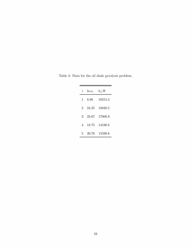
Table 2: Data for the oil shale pyrolysis problem.

i ln ai bi/R

1 8.86 10215.4

2 24.25 18820.5

3 23.67 17008.9

4 18.75 14190.8

5 20.70 15599.8

34

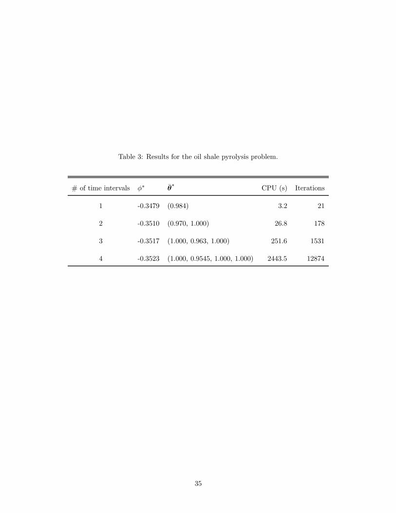
Table 3: Results for the oil shale pyrolysis problem.

# of time intervals φ∗ θ∗

CPU (s) Iterations

1 -0.3479 (0.984) 3.2 21

2 -0.3510 (0.970, 1.000) 26.8 178

3 -0.3517 (1.000, 0.963, 1.000) 251.6 1531

4 -0.3523 (1.000, 0.9545, 1.000, 1.000) 2443.5 12874

35