Deterministic K-Set Structure

Sumit Ganguly and Anirban Majumdersganguly,anirban@cse.iitk.ac.in

IIT Kanpur, India

Abstract. A k-set structure over data streams is a bounded-space data structure

that supports stream insertion and deletion operations and returns the set of (item,

frequency) pairs in the stream, provided, the number of distinct items in the stream

does not exceed k; and returns nil otherwise. This is a fundamental problem with

applications in data streaming [24], data reconciliation in distributed systems [22]

and mobile computing [28], etc. In this paper, we study the problem of obtaining

deterministic algorithms for the k-set problem.

1 Introduction

Consider scenarios where entities with identity arrive and depart in a critical zone, for ex-ample, persons with RF-tags, TCP connections to a given site, etc. The problem is to veryefficiently answer the following query:“ Are there at most k distinct entities (e.g., persons oritems or IP-addresses) in the critical zone, and if so, what are their identities?” Clearly, ifthere is enough memory to track all the entities, then, an O(n) space solution is the mostobvious one. The problem can be effectively solved using a k-set data structure, which is adata structure that (a) supports insertions and deletions of items in a stream or a multi-set,and, (b) supports a Retrieve operation that returns all the distinct items and their number ofoccurrences in the multi-set, provided, the number of distinct items is at most k; and returnsnil otherwise.

Applications of k-set structure arise in diverse areas, ranging from, practical applicationsin data streams and distributed computing [22, 28] to puzzles in recreational mathematics[5, 24]. In a distributed computing scenario, a host and a PDA may proceed asynchronouslywith their computations due to low (or non-existent) communication bandwidth betweenthem. Later a reconciliation mechanism is needed to synchronize a specific collection of bitsbetween the two hosts. Set reconciliation [22, 28] can be used as a mechanism that minimizesthe communication of bits between the two hosts. We discuss the set reconciliation problem inSection 2—here, we note that the k-set structure can be used to give a space-optimal solutionto the set and multi-set reconciliation problems. In a distributed computing environment,the k-set structure can be used for reconciling changes to shared structures, such as files,transaction logs, etc., with the minimum communication necessary.

1.1 Data Streaming Model

We use data streaming as the model for specifying the k-set structure. A data stream S isviewed as a sequence of records of the form (i, v), where, i is the identity of the data item thatis assumed to belong to the domain D = 1, 2, . . . , N and v is the change in the frequencyof i. For simplicity, we assume that v is integral, where, a positive value of v corresponds to v

insertions of i, and a negative value of v corresponds to v deletions of i. The frequency fi ofan item i is defined as the sum of the changes in the frequencies of i, that is, fi =

∑(i,v)∈S v.

At any given time, the multi-set corresponding to the stream is defined as (i, fi) | fi 6= 0.Let M denote an upper bound on the absolute value of the frequency of an item in thestream, that is, M ≥ fi, for each i ∈ S.

Data streams that allow insertions and deletions of items but allow item frequencies tobe both positive and negative are referred to as general update streams. A special case ofthe model arises when item frequencies in the data stream are always constrained to benon-negative. Such streams are referred to as strict update streams. In [24], Muthukrishnanrefers to the two models as the turnstile model and the strict turnstile model, respectively.Computations over non-negative update streams are studied in [3, 6, 8, 12, 17, 18]. The generalupdate streaming model has been used to detect changes in streams [7, 27].

1.2 K-set structure

We now formally two variants of the k-set structure, called strong and weak k-sets, respec-tively.

Definition 1. A strong k-set structure over a data stream is a structure that supports thefollowing three operations, (a) procedure Update, for updating the data structure correspond-ing to stream insertion and deletion operations, (b) procedure Count, that returns the numbern of items with non-zero frequencies, given that n ≤ k, (c) procedure Retrieve, that returnsthe multi-set S of (i, fi) pairs in the stream with fi 6= 0, provided, n ≤ k, and, (d) (c) proce-dure IsCard (Is Cardinality at most k?), that returns true if the number of distinct itemsin the stream (multi-set) is at most k and returns false otherwise. A weak k-set supportsall the above procedures, except, procedure IsCard. ut

K-set structures are readily designed by using classical dictionary structures includingheaps, binary search trees, red-black trees, AVL trees, hash tables, etc., that store the entireset S of items, and therefore, require Ω(|S|) = Ω(N) bits in the worst case. However, unlikethe generality of dictionary structures, a k-set structure only needs to return the set of itemsprovided this set is of size at most k. Therefore, there is a possibility of solving this problemin significantly lower space; as reinforced by the following lower bound argument. There are(Nk

)(2M−1)k possible multi-sets of of size k over the domain 1, 2, . . . , N such that |fi| ≤ M

and fi 6= 0. Each such multi-set must map to a distinct memory pattern of a deterministicalgorithm (otherwise, the algorithm makes an error in at least one of the inputs). Therefore,a deterministic k-set structure requires Ω(log(

(Nk

)(2M)k)) = Ω(k(log N

k + log M)) bits ofspace. We are interested in obtaining designs that use space that is close to this lower bound.

1.3 Previous work on Randomized k-set structures

A randomized strong k-set structure is a structure that uses random bits in the executionof the procedures Update, Retrieve and IsCard. Further, the Retrieve operation returns allthe n distinct items in the set when n ≤ k with high probability, and the IsCard operationreturns true or false correctly, with high probability. A randomized version of a weakk-set structure can be specified similarly.

Several constructions of randomized k-set structures are known. The Countsketch al-gorithm [4], extended by [7] to handle deletion operations, can be used to obtain a random-ized strong k-set structure. This structure uses space O(k(log k

δ )(log M +log N)2 log(log M +log N) log M) bits. An alternative strong k-set structure can be constructed using the Majority-based data structure [8] and the Count-Min sketch algorithm [6, 24]. Such a constructionuses space O(k log k

δ (log M + log N) log M) bits. The randomized k-set structure [10] usesO(k(log M + log N) log k

δ ) bits and is currently the most efficient randomized k-set struc-ture. The above three techniques are applicable to the general update streaming model (i.e.,fi Q 0). Muthukrishnan [24] (Theorem 15) describes a deterministic algorithm from [11] with

space complexity O(k2 log2 N log M log2 k) for identifying all top-k items (i.e., fi >P

j fj

k+1 ),assuming that there are at most k items in the stream. Given that there are at most k

items in the stream, a weak k-set structure can be used to retrieve all the items and theirfrequencies.

1.4 Contributions

We study the problem of designing k-set structures and present deterministic k-set struc-tures for the variants of the problem. Our results are the following. For the strict up-date streaming model, we present a near-optimal space construction for strong k-sets usingO(k(log M + log N)2) bits. The time complexity of procedures Retrieve, IsCard and Countare O(k4(log M + log N)2), O(k3) and O(k3) respectively. For the general update model, wepresent a weak k-set construction that uses O(k(log N + log M + log s)) bits to implementprocedure Count and O(k2(log M + log N)) bits to implement procedure Retrieve, where, s

is the sum of the absolute values of the updates to the stream, that is, s =∑

(i,v)∈ stream |v|.Alternatively, procedure Count can also be implemented using O(k2 log N + k log M) bits.We show that procedure IsCard requires Ω(N) bits in the general update streaming model.

1.5 Organization

The remainder of the paper is organized as follows. We discuss related problems in Section 2.Section 3 presents space lower bounds for strong k-sets. We present our k-set structure inSection 4 and discuss an implementation using finite fields. In Section 5, we discuss an im-plementation using real arithmetic with finite precision. Section 6 presents our experimentalresults. Finally, we conclude in Section 7.

2 Related Problems

The k-set problem has been posed and used earlier in different forms and in different ap-plications. We present two such examples, one from mobile communications (PDA synchro-nization) [22, 28] and another from recreational mathematics [24].

2.1 Set Reconciliation Problem

Set reconciliation [22, 28] is motivated by distributed systems where multiple hosts com-pute asynchronously in the face of unavailable and/or low-bandwidth network connectivityby temporarily sacrificing consistency. These problems arise in mobile computing [28], dis-tributed databases and distributed file systems [26, 9], etc.. Such systems typically requiresome mechanism for repairing whatever inconsistencies are introduced and set reconciliationis one of the mechanisms proposed for this problem. The problem is formalized as follows:given a pair of hosts A and B, each with a set of items SA and SB respectively from thedomain D = 1, 2, . . . , N − 1, what is the minimal amount of communication (in termsof numbers of bits exchanged and the numbers of rounds of messages) such that both A

and B are able to determine the union of their sets. The problem is to design solutionsthat require a communication complexity close to O(k log N), where, k is a known upperbound on the size of the symmetric difference between the sets of the two hosts, that is,k ≥ |SA − SB |+ |SB − SA|).

The set reconciliation problem can be easily solved using a weak k-set structure. The hostA inserts all its items with frequency 1 into the k-set structure and sends it to B. B deletesall its items from the k-set, and invokes the Retrieve function of the k-set to retrieve theidentity of the items. Since, the space complexity of a k-set structure is O(k log N) (in thiscase, M = 1), this gives an optimal communication complexity for the problem.

The work in [22] presents the following elegant technique to solve this problem. For sim-plicity, assume that SB ⊂ SA. First, A and B locally construct their respective characteristicpolynomials.

fA(z) =∏

u∈SA

(z − u) and fB(z) =∏

u∈SB

(z − u)

Then,

fA(z)fB(z)

=fA−B(z)fB−A(z)

(1)

Next, the polynomial fA is evaluated at k points (the authors [22] use the points a1 =−1, a2 = −2, . . . , ak = −k), not belonging to the domain D to obtain a vector (or a transform)FA = [fA(−1), . . . , fA(−k)]. The transform FA is then transmitted to B. In an analogousway, B computes its characteristic polynomial and evaluates the polynomial at the same k

distinct points, a1, a2, . . . , ak. By equation (1) (recall that for simplicity, we have assumedthat B ⊂ A), we can calculate the transform FA−B as follows.

FA−B =[fA(a1)fB(a1)

, · · · ,fA(ak)fB(ak)

]

Since, |A−B| is given to be of size at most k, the polynomial fA−B(z) is of degree at most k.The problem is now to invert the transform FA−B to obtain the polynomial fA−B , which canbe easily done using standard interpolation techniques. Since, fA−B(z) =

∏u∈SA−SB

(z−u),the factors of fA−B give the items in A−B. A single pass over the domain (field) is sufficientto retrieve all the factors. For a more efficient algorithm for this problem, see Section 4.2.

The authors [22] note that it is sufficient to perform the polynomial computations over afinite field of size q ≥ N (for simplicity, assume that N is a power of 2 and the finite fieldused is GF (N) of characteristic 2). Therefore, each member of the transform FA, namely,fA(uj), requires log N bits to be represented exactly. The total number of bits transmittedis the size of FA, which is bounded by k log N bits.

2.2 Multi-Set Reconciliation Problem

From the discussion above, it might appear that a k-set structure can be designed basedon the solution to the set reconciliation problem presented in [22]. However, the polynomialinterpolation technique presented above does not present an efficient solution to the followingmulti-set reconciliation problem. In the multi-set reconciliation problem, there are two hostsA and B, each having two multi-sets TA and TB , where, the items are from the domain0, 1, . . . , N−1 and the frequency of any item is at most M and is non-negative. The problemis to use the minimum number of communication bits and/or rounds of communication sothat each host knows the other’s multi-set.

We first show that the above problem is easily solved using a k-set structure. Supposethat we have an upper bound k on the number of distinct items that do not have the samefrequencies in the two multi-sets. Host A inserts its multi-set (i.e., (item, frequency) pairs)into a weak k-set and then transmits the k-set to B. B deletes its multi-set from the k-setand then retrieves the items and their frequencies by invoking procedure Retrieve. Items with

positive (resp. negative frequencies) have a higher frequency in the multi-set for B (resp. A)than in A (resp. B). This approach requires O(k(log M +log N)) bits of communication fromA to B.

The characteristic polynomial interpolation method can be adapted to solve the multi-setreconciliation problem as follows. Let fi and gi denote the frequency of item i (number ofoccurrences) in MA and MB , respectively. Then, the characteristic polynomials correspondingto the multi-sets MA and MB are as follows.

hA(z) =∏

i∈MA

(z − i)fi , hB(z) =∏

j∈MB

(z − j)gj

Therefore,

hA(z)hB(z)

=

∏i:fi>gi

(z − i)fi−gi

∏j:gj>fj

(z − j)gj−fj

For simplicity, assume that MB = φ and there are at most k distinct items in MA. Thecorresponding polynomial hA(z) = hA(z)

hB(z) can have degree kM . In general, in order to findthe coefficients of a degree m polynomial, it is necessary to maintain its value at m distinctpoints. The transform (or interpolation)-based procedure therefore has a space complexityof O(kM log N) bits.

2.3 Missing Numbers Puzzle

Muthukrishnan [24] presents the “Missing numbers puzzle” as a simple abstraction of aproblem over data streams. In the missing numbers puzzle, there are two parties, namely,Paul and Carole. Paul sends an arbitrary permutation of numbers from 1 to N , except atmost k of these numbers, to Carole. Carole is unaware of the permutation used by Paul. Theproblem for Carole is to find the missing numbers. Clearly, if Carole has N bits of memory,then she can trivially solve the problem by using it to remember all the numbers presentedto her. Therefore, the problem for Carole really is to find the missing numbers using as fewbits as possible. As pointed out by [24], this problem is an abstraction of problems in datastreaming.

[24] presents simple solutions for the case when there are one or two numbers are missing.A weak k-set structure easily solves the missing numbers problem, when there are at mostk items that are missing. Initially, Carole inserts all numbers 1 to N into a k-set, eachwith frequency 1. Next, for every number i that is supplied by Paul, Carole decrements thefrequency of i by 1, effectively, deleting i from the current set. The remaining set of items isexactly the set of missing numbers.

3 Lower Bounds

In this section, we discuss space lower bounds for k-set structure. As outlined in the intro-duction, a space lower bound of Ω(k(log N + log M − log k)) can be easily shown for thek-set structure. The argument is effective both for the streaming model where items havenon-negative item frequencies, and for the model where item frequencies can be both positiveor negative. We now consider space lower bounds for procedure IsCard, namely, the problemof testing deterministically whether there are k or less distinct items in the stream.

Lemma 1. Consider a streaming model where item frequencies can be both positive or neg-ative. Then, for any 1 ≤ k ≤ N

4 , a deterministic algorithm for testing whether the number ofdistinct items in the stream is at most k requires Ω(N) bits.

Proof. Let S be a family of sets of size N2 such that the distance between any pair of sets

in the family is at least N4 . Using simple counting techniques, it is easy to show that there

exists such families with size 2Ω(N).Let S and T be two such sets from the family. Construct two streams from S and T

respectively where the item frequency is 1 for each element in the corresponding set. Considerthe memory patterns of a k-set structure after processing the streams independently. Weclaim that the two memory patterns must be different for the following reason. Consider asequence of deletions of N

2 − k items from S that leaves S with k items. Since, S and T haveat most N

4 items in common, the same sequence of deletions applied to T leaves T with atleast N

2 −k distinct items (in which at least N4 −k have negative frequencies). It follows that

the space required by the k-set structure is at least Ω(log|S|) = Ω(N). ut

Lemma 1 justifies the terminology of weak and strong k-sets.

4 K-set structure

In this section, we present our design of a k-set structure. We keep s = 2k + 2 counters,denoted by l0, l1, . . ., l2k+1 that track the following quantities.

lr =∑

xi∈ stream

fixri , r = 0, 1, . . . , 2k + 1 (2)

The counters can be easily updated in the face of insertions and deletions occurring in thestream. For every update (xi, v) occurring in the stream, we update the rth counter as follows:

lr := lr + v · xri , for r = 0, 1, . . . , 2k + 1 .

We use the following notation in this section. Given n distinct items x1, x2, . . . , xn, each ofwhich lies in the interval 1 ≤ xi ≤ N , we let X = X(n) denote the n × n diagonal matrix

that has xi in its ith diagonal entry and zeros elsewhere. Given a set of n frequency values,f1, f2, . . . , fn, we let F denote the diagonal matrix whose ith diagonal entry is fi and is zeroelsewhere. Let f be the column vector [f1, f2, . . . , fn]T . That is,

X =

x1

x2

. . .

xn

F =

f1

f2

. . .

fn

and f =

f1

f2

...fn

.

For 1 ≤ n ≤ k and 0 ≤ r ≤ 2k − n, let V (r, n) denote the n× n matrix shown below. For agiven set of values x1, x2, . . . , xn, for brevity, we refer to V (0, n) as V , as follows.

V (r, n) =

xr1 xr

2 · · · xrn

xr+11 xr+1

2 · · · xr+1n

......

xr+n−11 xr+n−1

2 · · · xr+n−1n

V =

1 1 · · · 1x1 x2 · · · xn

x21 x2

2 · · · x2n

......

xn−11 xn−1

2 · · · xn−1n

The following identity is a direct consequence of the definition.

V (r, n) = V Xr (3)

Let w(s, r), Br and Cr denote the following r × 1 column matrix and r × r square matricesrespectively.

w(s, r) =

ls

ls+1

. . .

lr+s−1

Br =

l0 l1 . . . lr−1

l1 l2 . . . lr...

......

...lr−1 lr . . . l2r−2

, and Cr =

l1 l2 . . . lr

l2 l3 . . . lr+1

......

......

lr lr+1 . . . l2r−1

. (4)

4.1 Basic Properties

The main property of this structure is summarized in Lemmas 2 and 3. Lemmas 2 holds forstreaming models in which item frequencies could be both positive and negative.

Lemma 2. Suppose that there are n ≤ k distinct items in the stream. Then, (a) rank(Bk+1) =n, (b) the items x1, x2, . . . , xn are the eigenvalues of the matrix B−1

n Cn and, (c) the frequencyvector is given by f = V −1w(0, n).

Proof. Suppose there are n ≤ k distinct items x1, x2, . . . , xn in the stream, where, eachxi ∈ 0, 1, 2, . . . , N − 1, for i = 1, 2, . . . , n. Let V (r) = V (r, n) and w(r) = w(r, n), forr = 0, 1, 2, . . . , 2k + 1− n. Thus, equation (2) can be rewritten as follows.

V (r)f = V Xrf = w(r), r = 0, . . . , 2k + 1− n .

Since, the xi’s are non-zero and distinct, V (r) = V Xr is invertible for each value of 0 ≤ r ≤2k + 1− n. Therefore,

V XV −1w(r) = V Xr+1((V Xr)−1w(r)) = V Xr+1f = w(r + 1), 0 ≤ r ≤ 2k + 1 .

Let A denote the matrix V XV −1. The above set of equations can be expressed as

ABn = Cn (5)

Since A is in the eigen-decomposition form, X is the diagonal eigenvalue matrix of A. Inother words, the distinct items x1, . . . , xn are the eigenvalues of the matrix A′. Further,

Bn = [w(0) w(1) . . . w(n− 1)] = [V f, V Xf, V X2f, . . . , V Xn−1f ],

= V [f, Xf, X2f, . . . , Xn−1f ] = V FV T (6)

Since, V is invertible and none of the fi’s are 0, Bn is invertible, and therefore has rank n.Since Bn is the left n×n sub-matrix of Bk+1, rank(Bk+1) ≥ rank(Bn) = n. Let U denote

the (k + 1) × n matrix V (0, k + 1) and let U(j) be the (k + 1) × n matrix V (j, k + 1), for0 ≤ j ≤ k. Therefore, (2) can be equivalently written as: U(j)f = UXj = w(j, k + 1), forj = 0, . . . , k. Thus,

Bk+1 = [w(0, k + 1), w(1, k + 1), . . . , w(k, k + 1)] = U [f,Xf, . . . ,Xkf ] = UFUT .

Since, U and F each have rank n, it follows that rank(Bk+1) ≤ n. As shown earlier,rank(Bk+1) ≥ n. Therefore, rank(Bk+1) = n. ut

Lemma 2 can be used to design procedures Retrieve and Count for strong and potent k-setsrespectively, provided it is known that the number of distinct elements in the stream is atmost k. Lemma 2(a) and Lemma 3 provides the basis for testing whether a stream has k

or less distinct items. Notably, however, Lemma 3 is applicable only for streams where itemfrequencies are all non-negative (or, analogously, all non-positive).

Lemma 3. For strict update data streams (i.e., fi ≥ 0, for all i) there are n > k distinctitems in the stream with positive frequencies if and only if rank(Bk+1) = k + 1.

Proof. The if part is the statement of Lemma 2(a). Suppose there are n > k distinct itemswith positive frequencies. Let G denote the diagonal matrix with Gi,i set to the positivesquare root of fi. Therefore,

Bn = V FV T = V G2V T = (V G)(V G)T .

It follows that Bn is a positive definite matrix, and hence, all left most determinants of Bn arepositive. Since, n > k, in particular, det(Bk+1) > 0, and therefore, rank(Bk+1) = k + 1. ut

4.2 Implementing k-sets

In this section, we present a space efficient implementation of k-sets.Lemma 2 holds for any finite field of characteristic at least 2M and having N distinct

values. The number 2M is chosen to account for positive frequencies 1, . . . , M and negativefrequencies, −M, . . . ,−1. Choose an appropriate prime number p larger than 2M and let d

be the smallest integer ≥ 1, such that pr > N . Let F be the field GF (pr+1). The elements ofF can be naturally represented using O(log M + log N) bits. The counters, l0, . . . , l2k+1 areeach maintained as elements over F ; the total space requirement is O(k(log M + log N) bits.

Suppose it is given that the number of items in the stream n ≤ k (i.e., weak k-set), then,n can be found as rank(Bk+1). By Lemma 2, this property holds in general for data streamswhere item frequencies are both positive or negative. The identities of the items with non-zerofrequencies can be found as the eigenvalues of A. Since, iteratively convergent methods cannotbe used over finite fields, computing the eigenvalues of A over finite fields in general requiresthe computation of the roots of the characteristic polynomial F (z) = det(A− zI) = 0, whichis computationally expensive. For data streams where item frequencies can be both positiveand negative, the method of finding eigenvalues over R given in Section 5 can be applied. Ifitem frequencies cannot be negative, then the following algorithm (based on an applicationof dyadic intervals) can be used for finding the roots of the characteristic polynomial.

Finding roots of the characteristic polynomial. We now assume that item frequencies cannotassume negative values. Since there are n eigenvalues, the characteristic polynomial F (z) isof the form F (z) = α

∏a∈S(z − a), where, S is the set of items in the stream with non-zero

frequency and α is a constant. Let F be a field with characteristic larger than kM .Instead of maintaining a single set of 2k + 2 counters, we maintain a collection of L =

dlog|F |e − blog kc + 1 sets of counters, where each set consists of 2k + 2 counters. The sth

counter set is denoted as lsrr=0,1,...,2k+1, for 0 ≤ s ≤ L − 1. For 0 ≤ s ≤ L − 1, define afamily of functions hs : 0, 1, . . . , 2d − 1 → 0, 1, . . . , 2d−l − 1 as follows.

h0(a) = a and hs(a) = a÷ 2s

where, a÷2s is the quotient when the integer a is divided by the integer 2s. It follows directlythat, for any s ≥ 0 and given value of c = hs(a), there are exactly two distinct values of b

such that b = hs−1(a′). Corresponding to each stream update of the form (x, v), we updateeach of the s counter sets as follows.

lsr = lsr + (h(x))rv, 0 ≤ r ≤ 2k + 1, 0 ≤ s ≤ L− 1 .

Let f(s)a denote the frequency of item a at level s. Then, f

(s)a =

∑b:hs(b)=a fb. If a has positive

frequency fa > 0, then, f(s)hs(a) > 0 has positive frequency at level s, for 1 ≤ s ≤ L− 1 (vice-

versa may not be true). Let ns denote the number of distinct items with positive frequencies

at level s. Let A(s)ns , B

(s)ns and C

(s)ns respectively denote the corresponding matrices obtained

from the counters at level s, for s = 0, 1, . . . , L − 1. Let Fs(z) denote the characteristicpolynomial of A

(s)n , that is, Fs(z) = det(A(s)

ns − zI). By construction, we have the followingproperty

F (a) = 0 only if Fs(hs(a)) = 0 .

For each value of s starting from L and counting down to 0, we obtain a set of items of size atmost 2k that are potentially roots of Fs(z). At level L, there are at most k distinct items thatare then checked to see if Fs(as) = 0 (or equivalently, if A

(s)n − asI is singular). Therefore, at

each level, there cannot be more than k candidates that pass the above test. Each candidateitem a at level s corresponds to exactly 2 candidates at level s− 1; therefore, the number ofpotential candidates at any level is no more than 2k. Proceeding in this manner, we obtainthe set of items with positive frequencies at level 0.

The data structure maintains (2k + 2) counters for at most log|F | levels. Therefore, itsspace complexity is O(k(log N +log M)2) bits. Testing whether an item x is an eigenvalue canbe done by calculating the rank of A−xI, which can be done in time O(k3). Since there are atmost 2k candidate items at each level and there are log|F |− log k +1 = log M +log N − log k

levels, the time complexity of retrieval is O(k4(log M+log N)) field operations. We summarizethis discussion in the following lemma.

Lemma 4. A strong k-set structure can be designed for strict update data streams usingO(k(log M + log N)2) bits and operations over a finite field of size O(kM + N). The timecomplexity for procedure Retrieve is O(k4(log M +log N)) field operations and the time com-plexity for procedure IsCard is O(k3). For general update data streams, a weak k-set structurecan be designed with the space and time complexity mentioned above. ut

5 K-set structure using real arithmetic

Lemma 2 translates the problem of retrieving the elements to that of retrieving the eigen-values of a certain matrix. Today, optimized procedures for computing eigenvalues of realand complex matrices are widely available via packages such as LAPACK [1], MATLAB [21],MATHEMATICA [2], etc.. This makes it interesting and relevant to analyze the space andtime complexity of the procedure for retrieving the elements. In particular, we analyze thespace complexity and the number of bits of precision needed to count the number of itemswith non-zero frequency, and to retrieve the identity and frequency of those items without er-ror. We introduce a new parameter, called s, that is an upper bound on the number of updatesto the streams, that is, s =

∑(i,v)∈ stream |v|. The results in this section can be summarized

as follows. A strong k-set structure can be maintained using space O(k2 log N + k log M)bits. Procedure Count can also be implemented using space O(k(log M + log N + log s))

bits. Except for procedure IsCard, the other procedures are applicable to the general updatestreaming model (i.e., fi Q 0).

For r = 0, . . . , 2k + 1, the counter lr =∑

i fixri can have a value as large as MNr+1 and

can be maintained using (r+1)dlog Ne+dlog Me bits of storage. The space required to storethe counters l0, . . . , l2k+1 can be accounted as follows.

2k+1∑r=0

(rdlog Ne+ dlog Me) = Θ(k2 log N + k log M) bits.

Notation. The norm ‖M‖ of a matrix M denotes the 2-norm of M and is defined as thelargest eigenvalue of MT M in absolute value. The condition number [13, 29] of a matrix M

is denoted as κ(M) = ‖M‖‖M−1‖.

5.1 Precision for computing rank using Gaussian elimination.

The procedure Count can be implemented by determining the rank of the matrix Bk+1. Ifthis is done using the standard method of Gaussian elimination, then, the word size mustbe extended by the logarithm of the condition number of Bk+1 [13]. The condition numberof Bk+1 can be shown to be κ(Bk+1) = O(N4kMk222k). This implies that it is sufficient toextend the word size by log κ(Bk+1) = O(k log N + log m) bits.

5.2 Precision for computing A

The second matrix computation involves calculating A = CnB−1n , where, n ≤ k is the

number of items with non-zero frequencies in the stream. We use a simple variant of theQR-decomposition followed by back-substitution to obtain A.

Consider the matrix computation A = CnB−1n , where n ≤ k. For simplicity, we drop the

suffix n from the n× n matrices Cn and Bn. Note that A has the following form.

A = CB−1 =

0 1 0 0 · · · 00 0 1 0 · · · 0...

......

...0 0 0 0 · · · 1α1 α2 α3 α4 · · · αn

. (7)

where, the last row is denoted as the row vector αT = [α1, α2, . . . , αn]. Let cTn denote the nth

row of the matrix C. Equivalently,cTnB−1 = αT

or that, αT B = cTn . Taking transposes, we obtain the equivalent equation, BT α = cn. Since,

B is a symmetric invertible matrix, therefore, α is the unique solution to the equation

Bα = cn

where, cn is the nth column of C (since, C is symmetric). We now decompose B as B =QR using the classical QR decomposition algorithm [13, 29]. In this decomposition, Q is anorthonormal matrix and R is an upper triangular matrix satisfying ‖R‖ = ‖A‖. Therefore,Bα = cn is equivalent to QRα = cn, or, equivalently, Rα = QT cn. Since, R is an uppertriangular matrix, α is obtained using back substitution. Due to limited precision, the matrixR is calculated as R + ∆R. If floating point calculation is used up to s2 bits of precision,then, ‖∆R‖ ≤ 2−Ω(s2)‖R‖. Therefore, the possible error ∆α in the calculation of α is givenby

‖∆α‖ ≤ κ(R)‖∆R‖‖R‖ ‖α + ∆α‖ ≤ 2−Ω(s2)κ(B)‖α + ∆α‖ (8)

It follows that the error term ‖∆α‖ is negligible compared to α if s2 is O(log(κ(B))).By Lemma 2, we have B = V FV T . By Gershgorin circle theorem, ‖V ‖ = O(N2n+1) and

‖V T ‖ = O(N2n+1). Clearly, ‖F‖ ≤ M . Therefore, ‖B‖ = O(N2n+1M). Further, ‖V −1‖ ≤O(Nn+1) and ‖(V −1)T ‖ = O(Nn+1) (see Appendix B). Therefore, κ(B) = O(N4n+2M).Since n ≤ k, it follows that if s2 = O(k log N + log M), then, from equation (8), the errorterm ∆α is negligible. Let ∆A denote the error matrix for A, then, by construction (seeequation (7))

∆A = en(∆α)T

where, en is the n× 1 unit column vector with 1 in row n and 0 elsewhere. Therefore,

‖∆A‖ ≤ ‖∆α‖ ≤ 2−Ω(s2)κ(B)‖α‖ . (9)

Since, ‖A‖F ≤ √n‖A‖, it follows that,

‖A‖F = n− 1 + ‖a‖ ≤ √n‖A‖, or that, ‖a‖ ≤ √

n‖A‖ .

Substituting in (9), we have,

‖∆A‖ ≤ 2−Ω(s2)√

nκ(B)‖A‖

Therefore, A is computed to sufficient precision given the following condition.

if s2 = O(log n + log κ(B)) = O(k log N + log M)

then ‖∆A‖ ≤ N−Ω(k)M−Ω(1)‖A‖ .

We summarize the above discussions in the following lemma.

Lemma 5. There exists a weak k-set structure for the general update streaming model (i.e.,fi Q 0) using real arithmetic with finite precision that uses O(k2 log N +k log M) bits of spacefor maintaining the counters. The procedures Count and Retrieve can be implemented usingO(k log N + log M) bits of floating point precision. ut

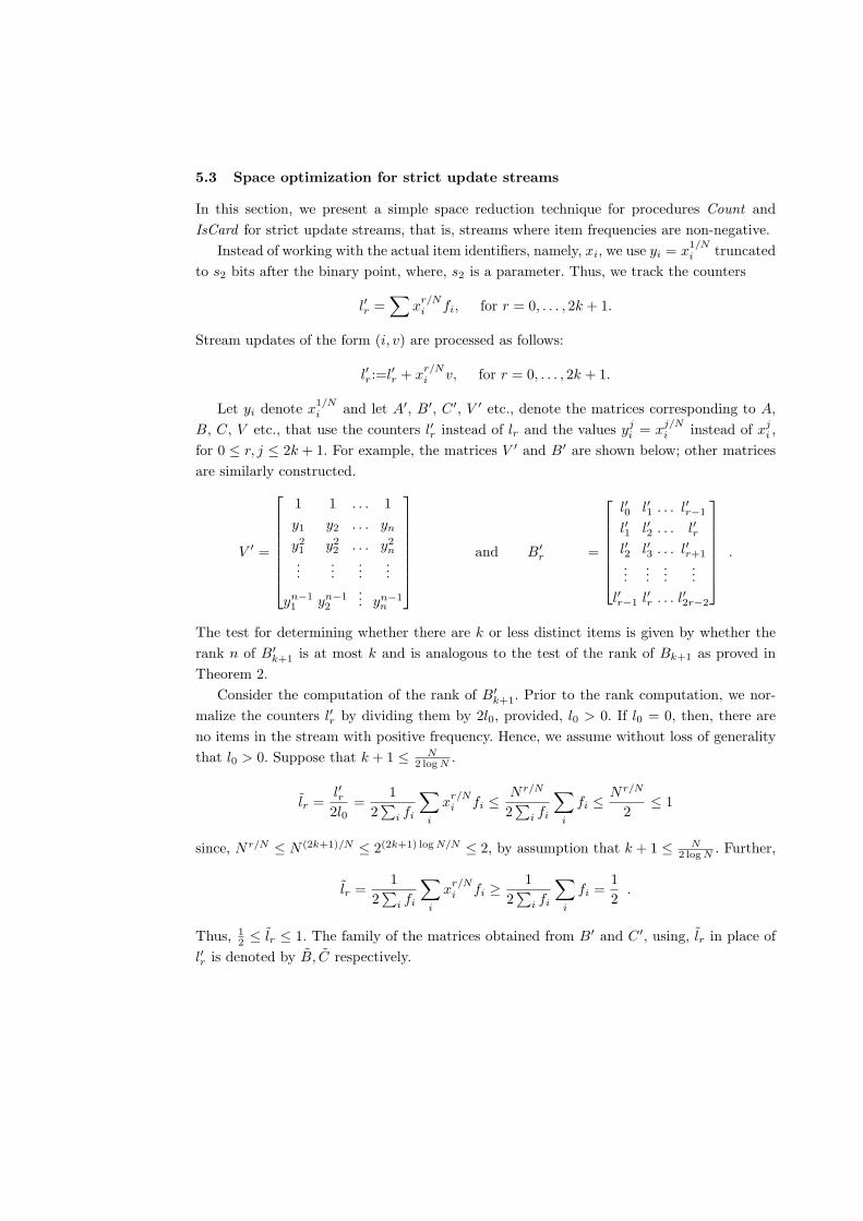
5.3 Space optimization for strict update streams

In this section, we present a simple space reduction technique for procedures Count andIsCard for strict update streams, that is, streams where item frequencies are non-negative.

Instead of working with the actual item identifiers, namely, xi, we use yi = x1/Ni truncated

to s2 bits after the binary point, where, s2 is a parameter. Thus, we track the counters

l′r =∑

xr/Ni fi, for r = 0, . . . , 2k + 1.

Stream updates of the form (i, v) are processed as follows:

l′r:=l′r + xr/Ni v, for r = 0, . . . , 2k + 1.

Let yi denote x1/Ni and let A′, B′, C ′, V ′ etc., denote the matrices corresponding to A,

B, C, V etc., that use the counters l′r instead of lr and the values yji = x

j/Ni instead of xj

i ,for 0 ≤ r, j ≤ 2k + 1. For example, the matrices V ′ and B′ are shown below; other matricesare similarly constructed.

V ′ =

1 1 . . . 1y1 y2 . . . yn

y21 y2

2 . . . y2n

......

......

yn−11 yn−1

2

... yn−1n

and B′r =

l′0 l′1 . . . l′r−1

l′1 l′2 . . . l′rl′2 l′3 . . . l′r+1

......

......

l′r−1 l′r . . . l′2r−2

.

The test for determining whether there are k or less distinct items is given by whether therank n of B′

k+1 is at most k and is analogous to the test of the rank of Bk+1 as proved inTheorem 2.

Consider the computation of the rank of B′k+1. Prior to the rank computation, we nor-

malize the counters l′r by dividing them by 2l0, provided, l0 > 0. If l0 = 0, then, there areno items in the stream with positive frequency. Hence, we assume without loss of generalitythat l0 > 0. Suppose that k + 1 ≤ N

2 log N .

lr =l′r2l0

=1

2∑

i fi

∑

i

xr/Ni fi ≤ Nr/N

2∑

i fi

∑

i

fi ≤ Nr/N

2≤ 1

since, Nr/N ≤ N (2k+1)/N ≤ 2(2k+1) log N/N ≤ 2, by assumption that k + 1 ≤ N2 log N . Further,

lr =1

2∑

i fi

∑

i

xr/Ni fi ≥ 1

2∑

i fi

∑

i

fi =12

.

Thus, 12 ≤ lr ≤ 1. The family of the matrices obtained from B′ and C ′, using, lr in place of

l′r is denoted by B, C respectively.

Clearly, with infinite precision, both techniques, namely, working with the matrices B, C

etc., and working with the matrices B′, C ′ etc. are equivalent. However, we show that byusing fixed point arithmetic using word size of O(log m + log N + log s) bits, the problem ofdetermining the rank of B′ can be solved exactly for data streams with at most s updates.

We use the QR-decomposition algorithm on the columns of Bk+1 for computing its rank[15] using standard fixed point arithmetic, that is, by truncating underflows to 0 and ignoringoverflows. Lemma 6 follows from the standard properties of the QR-decomposition procedureand is presented in Appendix A.

Lemma 6. Suppose that the rank of B is computed using fixed point arithmetic using wordsize of s2 = 32(log N +log M +log s) bits before and after the binary point. Further, any valuethat is smaller (in absolute value) than 1

2m2N16 is deemed to be 0. Then, the QR procedureexactly computes the rank of B.

Proof. See Appendix A. ut

The main consequence of Lemma 6 is Lemma 7, which states that a k-set structure can bedesigned for strict update streams using real arithmetic that requires space O(k(log M +log N +log s)) bits for implementing procedures Count and IsCard. However, in this method,procedure Retrieve still requires O(k2 log N + log M) bits of space for computing the eigen-values.

Lemma 7. There exists a design of a k-set structure for the strict update streaming modelbased on real arithmetic that uses space O(k (log M + log N + log s)) bits for implementingprocedures Count and IsCard. The time complexity of these procedures is O(k3) operationsover fixed point numbers with O(k(log M + log N + log s)) bits before and after the binarypoint. ut

5.4 A Las Vegas type optimization

The worst-case space complexity of the k-set structure was analyzed in Theorem 5 asO(k2 log N +k log m+k log s) bits. The worst-case occurs when the k-items are N−k,N−k+2, . . . , N − 1, respectively. This “lack of separation” among the items leads to the worst-caseprecision requirement of the algorithm. In this section, we present a simple Las Vegas type ofoptimization to increase the gap between the items, thereby, reducing the space requirementin practice.

Consider a family of permutations Π over the domain 1, 2, . . . , N that are approxi-mately k-wise independent with relative error ε. Constructions of permutation families canbe found in [20, 25, 14, 16, 19]. A brief overview of work in approximately k-wise independentpermutations is presented in Appendix C.

Let π be a randomly chosen permutation from Π. Each item xi over the stream is firsttransformed into π(xi), and then inserted into the k-set structure. The Retrieve operationretrieves the hash values, π(x1), . . . , π(xk), that are then inverted to retrieve the originalitems x1, . . . , xk. The choice of the random hash function increases the average gap betweenthe items and prevents an adversary from consistently choosing the worst-case input forthe algorithm. The expected number of bits of precision and therefore, the expected spacecomplexity of the Las Vegas variant is lower than the original algorithm. It is called the LasVegas type of optimization, since, the space and time required by the algorithm is a randomvariable, although, the algorithm deterministically gives the correct answer [23]. Lemma 8presents upper bounds on the expected space complexity of implementing a k-set structureusing this method and is the counterpart to Lemma 5. It quantifies the expected economyin space complexity obtained by using this method over the deterministic method (viz.,O(k2 + k log M + k log s) bits versus O(k2 log N + k log M) bits).

Lemma 8. The Las Vegas technique implements a weak k-set structure for the general up-date streaming model using O(k2 + k log M + k log s) bits on expectation.

Proof. See Appendix B. ut

6 Experimental Study

In this section we present the results of preliminary experiments that we performed to com-pare the space required by the k-set structure implemented using finite precision arithmeticover reals against its theoretical complexity. Our experiments were performed on Sun E250Server having Eultra Sparc II, 400 MHz Dual processor with 1GB RAM and 18GB Harddisk with the Solaris 8 operating system using the Matlab software version 6.0.0.88.

The first set of experiments test the worst-case of the k-set solution, (i.e, xi = N − k + i,for i = 0, 1, 2, . . . k − 1), for N = 232 and varying k from 8 to 256. The frequencies of itemsare taken as 1 in this case. The space requirement (= bits of precision × k log N) for theoriginal and the Las Vegas variant of the k-set solution is measured and plotted as a functionof k, as shown in Figure 1. The experimental results indicate that the space complexity of thebasic k-set structure is sub-quadratic, thereby, showing that in practice, the k-set structuremethod works significantly better than predicted. Figure 1 also shows the space required bythe Las Vegas variant (measured as the average over 10 runs, for each value of k), that is, asexpected, consistently superior to the original solution.

Our second set of experiments evaluate the accuracy of the frequency estimation bychoosing 32-bit frequency values at random and associating each frequency value to a numberbetween N − k + 1, . . . , N (the worst case input, without initial randomization). Figure 2presents a graph that measures the accuracy of frequency estimation as function of the

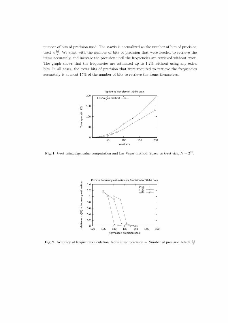
number of bits of precision used. The x-axis is normalized as the number of bits of precisionused × 16

k . We start with the number of bits of precision that were needed to retrieve theitems accurately, and increase the precision until the frequencies are retrieved without error.The graph shows that the frequencies are estimated up to 1.2% without using any extrabits. In all cases, the extra bits of precision that were required to retrieve the frequenciesaccurately is at most 15% of the number of bits to retrieve the items themselves.

0

50

100

150

200

50 100 150 200

Tot

al s

pace

(in K

B)

k-set size

Space vs Set size for 32-bit data

Las Vegas method

Fig. 1. k-set using eigenvalue computation and Las Vegas method: Space vs k-set size, N = 232.

0

0.2

0.4

0.6

0.8

1

1.2

1.4

120 125 130 135 140 145 150rela

tive

erro

r(%

) in

freq

uenc

y es

timat

ion

Normalized precision scale

Error in frequency estimation vs Precision for 32-bit data

k=16k=32k=64

Fig. 2. Accuracy of frequency calculation. Normalized precision = Number of precision bits × 16k

7 Conclusions

We present space and time-efficient, deterministic k-set structures that are nearly space-optimal. The problem of designing more time-efficient k-set structures is open.

References

1. “LAPACK: The Linear Algebra Package”. Available from “www.netlib.org/LAPACK”.

2. “MATHEMATICA”. WolframResearch.

3. Noga Alon, Yossi Matias, and Mario Szegedy. “The space complexity of approximating frequency

moments”. Journal of Computer Systems and Sciences, 58(1):137–147, 1998.

4. M. Charikar, K. Chen, and M. Farach-Colton. “Finding frequent items in data streams”. In

Proc. ICALP, 2002.

5. V. Chauhan and A. Trachtenberg. “Reconciliation puzzles”. In Proc. IEEE GLOBECOM, 2004.

6. G. Cormode and S. Muthukrishnan. “An improved data stream summary: The Count-Min

sketch and its applications”. In Proc. LATIN, pages 29–38, 2004.

7. G. Cormode and S. Muthukrishnan. “What’s New: Finding Significant Differences in Network

Data Streams”. In Proc. IEEE INFOCOM, 2004.

8. Graham Cormode and S. Muthukrishnan. “What’s Hot and What’s Not: Tracking Most Frequent

Items Dynamically”. In Proc. ACM PODS, pages 296–306, 2003.

9. A.J. Demers, D. H. Greene, C. Hause, W. Irish, and J. Larson. “Epidemic algorithms for

replicated database maintenance”. In Proc. ACM PODC, pages 1–12, August 1987.

10. S. Ganguly. “Counting distinct items over update streams”. In Proc. ISAAC, pages 505–514,

2005.

11. L. Gasieniec and S. Muthukrishnan. “Deterministic algorithm for estimating heavy-hitters on

Turnstile data streams”. Manuscript, 2005.

12. Anna Gilbert, Sudipto Guha, Piotr Indyk, Yannis Kotidis, S. Muthukrishnan, and Martin

Strauss. “Fast Small-space Algorithms for Approximate Histogram Maintenance”. In Proceed-

ings of the 34th ACM Symposium on Theory of Computing (STOC), 2002, Montreal, Canada,

May 2002.

13. Gene H. Golub and Charles F. Van Loan. “Matrix Computations”. J. Hopkins Univ. Press, 3rd

edition, 1996.

14. W. T. Gowers. “An almost m-wise independent random permutation of the cube”. Combina-

torics, Probability and Computing, 5(2):119–130, 1996.

15. K. M. Hoffman and R. Kunze. “Linear Algebra”. Prentice-Hall, 2nd Ed., 1971.

16. S. Hoory, A. Magen, S. Myers, and C. Rackoff. “Simple permutations mix well”. pages 770–781.

17. P. Indyk and D. Woodruff. “Optimal Approximations of the Frequency Moments”. 2005.

18. Piotr Indyk. “Stable Distributions, Pseudo Random Generators, Embeddings and Data Stream

Computation”. In Proceedings of the 41st Annual IEEE Symposium on Foundations of Computer

Science, pages 189–197, Redondo Beach, CA, November 2000.

19. E. Kaplan, M. Naor, and O. Reingold. “Derandomized Constructions of k-Wise (Almost) Inde-

pendent Permutations”. pages 354–365.

20. M. Luby and C. Rackoff. “How to construct pseudorandom permutations and pseudorandom

functions”. SIAM J. Comp., 17(1):373–386, 1988.

21. The Mathworks, Natick, MA, USA. “MATLAB 7.1”.

22. Y. Minsky, A. Trachtenberg, and R. Zippel. “Set Reconciliation with Nearly Optimal Commu-

nication Complexity”. IEEE Trans. Inf. Theory, 49(9):2213–2218, 2003.

23. R. Motwani and P. Raghavan. “Randomized Algorithms”. Cambridge University Press, 1995.

24. S. Muthukrishnan. “Data Streams: Algorithms and Applications”. Foundations and Trends in

Theoretical Computer Science, Vol. 1, Issue 2, 2005.

25. M. Naor and O. Reingold. “On the Construction of Pseudorandom Permutations: Luby-Rackoff

Revisited”. J. Cryptology, 12(1):29–66, 1999.

26. M. Satyanarayanan. “Scalable, Secure, and Highly Available Distributed File Access”. IEEE

Computer, 23(5), May 1990.

27. R. Schweller, Z. Li, Y. Chen, Y. Gao, A. Gupta, Y. Zhang, P. Dinda, M-Y. Kao, and G. Memik.

“Monitoring Flow-level High-speed Data Streams with Reversible Sketches”. In Proc. IEEE

INFOCOM, 2006.

28. D. Starobinski, A. Trachtenberg, and S. Agarwal. “Efficient PDA synchronization”. IEEE Trans.

on Mob. Comp., 2(1):40–51, 2003.

29. Gilbert Strang. “Introduction to Linear Algebra”. Wellesley-Cambridge Press, 2nd ed., 1998.

A Proof of Lemma 6

In this section, we present a proof of Lemma 6. In this proof, the dependence on the size ofthe stream, namely, s =

∑(i,v)∈ stream|v|, is omitted for simplicity. It is readily incorporated

into the statement of the lemma using the following observation. If the precision kept is s2

bits, then, after s stream updates operations, the error is at most s2−s2 . This implies thatafter s operations, the precision decreases by effectively s2 − log s bits. We use this modifiedvalue of s2 as the starting point.

Let Bk+1 = [b0, b1, . . . , bk] denote the k + 1 columns of B. If b0 = 0, then, the rank is0 and the stream is empty. Otherwise, none of the bi’s is the zero vector (since each of thecounters lr is positive). Let bT

j · bi denote the inner product of the vectors bj and bi. Weconstruct the following sequence of vectors (standard Graham-Schmidt ortho-normalization)using fixed-point arithmetic (that truncates underflows to 0 and ignores overflows) usings1 = 32(log m + log N) bits before and s2 = 32(log m + log N) bits after the binary point.

v0 =b0

‖b0‖v′i = bi − (vT

0 · bi)v0 − (vT1 · bi)v1 − · · · − (vT

i−1 · bi)vi−1

i = 1, 2, . . . , k

vi =v′i‖v′i‖

, i = 1, 2, . . . , k (10)

A vector vi is deemed to be a non-zero vector if any of its coordinates has at least one bitwhich is set to 1 among the bits before the binary point or among the first 1 + dlogDe bitsafter the decimal point, where, D = (k + 1)m2N16. Otherwise, vi is deemed to be the zerovector. The algorithm keeps a set of vectors vi which are deemed to be nonzero and returnsthe size of the set(size of the orthogonal basis) as the rank of Bk+1. The following analysisshows that there are no errors caused by limited precision in the above algorithm.

Analysis of rank computation

For the vector vi, the algorithm finds the component of bi along each of the vectors b1, b2, . . . bi−1.

The component of bi along vj is calculated simply as vTj bi

‖vj‖ vj which is equal to (vTj ·bi)vj since

vj is normalized.By induction, the vectors, b0, . . . , bi−1 are all independent, otherwise, thealgorithm would have terminated earlier. Thus vi computes the residual component of bi aftersubtracting the components along each of b0, b1, . . . , bi−1. Assuming infinite-precision, it isclear that if bi is linearly dependent on the first i vectors, then, after removing its componentsalong those vectors, the residual vector vi would be zero. Equation (10) can be equivalentlywritten in scalar form (that is, an equation for each of the k +1 coordinates of vi) as follows.

(vi)j = li+j −j+i−1∑

r=j

lr lr−j + lr+1 lr−j+1 + · · ·+ lr+k lr−j+k

l2r−j + l2r−j+1 + . . . l2r−j+k

· lr, (11)

for j = 1, . . . , k + 1.

Let yi denote yi = x1/Ni truncated to s2 bits after the binary point. Thus, |yi−yi| ≤ 2−s2 .

Hence |yri − yr

i | ≤ k ·N 2kN · 2−s2 for r = 0, 1, . . ., 2k+1 . Let’s call this value as δ. Due to

truncation after s2 bits beyond the binary point, each of the counters lr has an error of atmost k ·δ. Each multiplication of two of the lr’s introduces an additive error of at most 3k3 ·δ.Consider the numerator of any summand of (11). There are a total of k + 1 multiplicationsand k additions; thus the total error introduced is at most 3 · k4 · δ. The denominator is atmost k and incurs truncation error that is bounded in absolute value by 3 ·k4 · δ (since, thereare k multiplications and k additions, each of which incurs an error of at most 3 ·k3 ·δ). Thus,the total additive error in the calculation of the summand in equation (11) for a given valueof r is bounded by U+3·k4·δ

V−3·k4·δ − UV , where, U and V are the correct values for the numerator

and the denominator for an index r. Since, 1m ≤ U, V ≤ (k + 1), the above error can be

bounded in absolute value by 10k2 ·m2 · δ if s2 ≥ 6 + 5 log k + log m + 2kN log N . There are

i ≤ k + 1 summands in the calculation of (vi)j ; the error due to truncation of (vi)j is atmost ε = 10k3 ·m2 · δ. By equation (11), the value of the fraction for each summand indexr is at least 1

m2 . Therefore, the minimum absolute value of (vi)j , if it is not zero, is at leastγ = 1

m − 1m2 . Therefore, by choosing s2 ≥ 6 + 6 log k + 3 log m + 2k

N · log N gives γ > ε .

The maximum absolute value of (vi)j is at most m(k + 1)2 + k. With the given choice ofs2 = 32(log m + log N), there is no overflow error. Thus, non-zero vi’s are never deemed tobe zero vectors, and vice-versa.

B Proof of Lemma 8

By Lemma 9, it follows that ‖V ‖ = O(n2). We now calculate a bound on the expected valueof ‖V −1‖.Lemma 9. E

[‖V −1‖

]≤ n28n.

Proof. Let zj = x1/Nj . The (i, j)th entry of the matrix V ′ is given by zi

j , 0 ≤ i ≤ n − 1 and1 ≤ j ≤ n. Denote V ′T by W . Clearly, by definition of Frobenius norms,

‖V ′−1‖F = ‖(V ′−1)T ‖F = ‖(V ′T )−1‖F = ‖W−1‖F .

By direct calculation of the inverse of Vandermonde matrix,

(W−1)i,j = coefficient of ti in

∏ns=1s 6=j

(t− zs)∏n

s=1s 6=j

(zj − zs)

Consider the jth column of W−1. The sum of the absolute values of the entries in this columncan be obtained as follows.

n∑

i=1

|Wi,j | =n∑

i=1

∏ns=1s 6=j

(1 + zs)∏n

s=1s 6=j

(|zj − zs|)

We now assume that the zi’s are random, independently chosen and distinct in the domain1, . . . , N. Taking expectations and using linearity of expectation,

E

[n∑

i=1

|Wi,j |]

=n∑

i=1

E

∏ns=1s 6=j

(1 + zs)∏n

s=1s6=j

(|zj − zs|)

(12)

For a fixed value of xj , the value of each of xs, for s 6= j, is independent over the domain1, . . . , N − xj. Therefore,

E

∏ns=1s 6=j

(1 + zs)∏n

s=1s 6=j

(|zj − zs|)

=

n∏s=1s6=j

E[

1 + zs

|zj − zs|]

(13)

Since, 12 ≤ zs ≤ 1, 1 + zs ≤ 2. We therefore have,

E[

1 + zs

|zj − zs|]≤ E

[2

|zj − zs|]

Recall that zj = x1/Nj and zs = x

1/Nj , where, 1 ≤ xj , xs ≤ N , and xj 6= xs. For each

fixed value of xj , |xj − xs| takes values between 1 and N − 1 with probability at most 2N−1 .

Therefore,

E[

1|zj − zs|

]≤

N−1∑

|xj−xs|=1

2N − 1

1|zj − zs| .

For a fixed value of y = |xj − xs|, the smallest value of |zj − zs| occurs when xs = 1 andxj = (y + 1)1/N . It follows that,

E[

1|zj − zs|

]≤

N−1∑y=1

2(N − 1)

1((y + 1)1/N − 1)

.

By simplifying the summation in the RHS, we obtain,

E[

1|zj − zs|

]≤ 2

N − 1

(1

21/N − 1+

∫ N−1

y=2

dy

y1/N − 1

)(14)

Note that

ln 21/N =ln 2N

≥ ln(

1 +ln 2N

).

Therefore,

21/N ≥ 1 +ln 2N

or, that 21/N − 1 ≥ ln 2N

. (15)

Substituting in (14), and replacing the variable of integration by t = y1/N , we have,

E[

1|zj − zs|

]≤ 2N

(N − 1) ln 2+

2N − 1

∫ N1/N

t=21/N

tN−1dt

t− 1. (16)

Simplifying the integral in the RHS

∫ N1/N

t=21/N

tN−1dt

t− 1=

∫ N1/N

t=21/N

(1 + t + t2 + . . . + tN−2)dt +∫ N1/N

t=21/N

dt

1− t

=(

t +t2

2+

t3

3+ · · ·+ tN−1

N − 1

)∣∣∣∣N1/N

21/N

+ lnN1/N − 121/N − 1

≤ HN−1 + ln1

21/N − 1≤ HN−1 + 2 .

where, HN−1 denotes the (N − 1)th harmonic number, namely, 1 + 12 + 1

3 + · · · + 1N−1 .

Substituting in (16)

E[

1|zj − zs|

]≤ 2N

(N − 1) ln 2+

2(HN−1 + 1)N − 1

≤ 8m .

Substituting in (13) and then in (12), we have,

E[‖W−1‖F

]= E

n∑

j=1

n∑

i=1

|Wi,j | ≤

n∑

j=1

n∑

i=1

8n ≤ n28n ut

Lemma 10. κ(B′) ≤ n882nM .

Proof. Recall that B = V F V T . ‖V ‖ ≤ ‖V ‖F ≤ n2, since, each of the entries is at most 1.The same argument holds for ‖V T ‖F . Further,

‖F‖ ≤ M and ‖F−1‖ ≤ 1

Therefore,‖B‖ ≤ ‖V ‖‖F‖‖V T ‖ ≤ n4M

By Lemma 9,‖B−1‖ ≤ ‖V −1‖‖F−1‖‖(V T )−1‖ ≤ n882n .

Taking products,

κ(B) = ‖B‖‖B−1‖ ≤ n882nM ut

Proof (Of Lemma 8). The precision required for the eigenvalue computation and for comput-ing the inverse is O(log κ(B)) = O(n + log M) = O(n + log M) = O(k + log M). Since thereare 2k + 1 counters, the total space complexity is (2k + 1)O(k + log M) = O(k2 + k log M)bits. The Las Vegas method stores the counters l′r instead of lr. Therefore, after a total ofs updates, the loss in precision is log s bits, therefore, the total number of bits required isO(k2 + k log M + k log s) bits. ut

C Review of approximate t-wise independent permutations

A family of permutations Π over F is said to be approximately t-wise independent with errorparameter δ, provided, for any Turing machine M that has access to a random permutationπ and makes at most t calls to π, M cannot distinguish whether π is chosen uniformly atrandom from Π or uniformly at random from U , with probability more than δ. Here, U isthe set of all permutations over F . In other words, for any Turing machine M meeting thecriterion above, and for every input I, the following condition holds.

∣∣Prπ∈RΠ M succeeds on I −Prπ∈RU M succeeds on I∣∣ ≤ δ

where, the notation π ∈R Π indicates that π is chosen uniformly at random from Π (re-spectively, U). We are more interested in permutation families that are approximately t-wise

independent with relative error ε, where, ε < 1. That is, for any Turing machine with accessto a random permutation π and that makes at most k calls to π, the following conditionholds for every input I.

∣∣Prπ∈RΠ M succeeds on I∣∣ ∈ (1± ε)Prπ∈RU M succeeds on I

A simple calculation shows that if Π is approximately t-wise independent with relative errorε, then its absolute error δ = O(ε · 2−mt).

The Fiestel permutations based approaches, such as Luby and Rackoff, Naor and Reingold[20, 25] have errors of the form of δ = t2

2m/2 , that are considerably large and inadequate. The3-bit mixed permutations of Gowers [14] with improvements due to Hoory, Magen, Myersand Rackoff [16] require space and time O((m3t2 + m2t log 1

ε ) log m) bits and m-bit wordoperations to evaluate π(x), respectively. The construction of Kaplan, Naor and Reingold[19] results in ε-approximate t-wise independent permutation family requiring O(mt + log 1

ε )bits. However, the time complexity of the Kaplan, Naor, Reingold construction is a veryhigh-degree of polynomial in m and t (also discussed by the authors in [19] Section 6.1).

In data stream processing, π has to be applied to each arriving record, and since, recordsarrive at a rapid rate, π(·) must be very efficiently computable, which, unfortunately, is notthe case with Kaplan, Naor and Reingold’s construction. We therefore use the construction ofHoory, Magen, Myers and Rackoff since its time-complexity is relatively better, but remarkthat it is desirable to obtain constructions of approximate t-wise independent permutationfamilies that are more suited for high-speed data stream processing.