developing a biosensor with applying kalman filter …
TRANSCRIPT

DEVELOPING A BIOSENSOR WITH APPLYING KALMAN
FILTER AND NEURAL NETWORK TO ANALYZE DATA FOR
FUSARIUM DETECTION
A Thesis Submitted to the College of
Graduate and Postdoctoral Studies
In Partial Fulfilment of the Requirements
For the Degree of Doctor of Philosophy
In the Department of Electrical and Computer Engineering
University of Saskatchewan
By
Son Ng. Pham
Saskatoon, Saskatchewan, Canada
© Son Ng. Pham, February, 2020. All rights reserved.

i
Permission to Use
In presenting this thesis in partial fulfilment of the requirements for a Postgraduate degree from
the University of Saskatchewan, it is agreed that the Libraries of this University may make it freely
available for inspection. Permission of copying this thesis in any manner, in whole or in part, for
scholarly purposes may be granted by the professor who supervised my thesis work or, in their
absence, by the Head of the Department of Electrical and Computer Engineering or the Dean of
the College of Graduate and Postdoctoral Studies in which my thesis work was done. It is
understood that any copying or publication or use of this thesis or parts thereof for financial gain
shall not be allowed without the written permission of the author. An appropriate recognition shall
be given to me and to the University of Saskatchewan in any scholarly use which may be made of
any material in my thesis.
Requests for permission to copy or to make other use of material in this thesis in whole or part
should be addressed to:
Head of the Department of Electrical and Computer Engineering
57 Campus Drive
University of Saskatchewan
Saskatoon, Saskatchewan, Canada
S7N 5A9
OR
Dean College of Graduate and Postdoctoral Studies University of Saskatchewan 116 Thorvaldson Building, 110 Science Place Saskatoon, Saskatchewan S7N 5C9 Canada

ii
Abstract
Early detection of Fusarium is arduous and highly desired as the detection assists in protecting
crops from the harmful potential of plant pathogens which affect the quality and quantity of
agriculture products. The thesis work concentrates on searching an approach for Fusarium spore
detection and developing portable, reliable and affordable Fusarium detection device. The system
can also promptly and continuously sample and sense the presence of the fungus spores in the air.
From the investigation of the Fusarium oxysporum Chlamydospores by ATR-FTIR spectroscopy,
a distinct infrared spectrum of the Chlamydospore was collected. There are two typical infrared
wavelengths can be used for Fusarium detection: 1054cm-1 (9.48µm) and 1642cm-1 (6.08µm).
Infrared (IR) light is a form of electromagnetic wave which its wavelength ranges from around
0.75µm to 1000µm and it is invisible to human eyes. To be familiar with the light concepts and
quantities, it is necessary to start working with the visible light which is also a form of
electromagnetic wave with the wavelength range from about 0.3µm to 0.75µm. A visible
spectrometer, which automatically corrects data error caused by unstable light, was built. By using
the Kalman filter algorithm, Matlab simulations and training program, the appropriate coefficients
to apply to the Kalman corrector were found. The experiments proved that the corrector in the
visible spectrometer can reduce the data error in the spectra at the order of 10 times.
From the knowledge of working with the visible spectrometer and visible light, the task of
searching the detecting approach and building the device in the IR spectrum was reconsidered.
The Fusarium detection device was successfully built. Among other components to build the
device, there are two essential thermopiles and one infrared light source. The infrared light source
emits an IR spectrum from 2µm to 22µm. The two thermopiles working on the IR wavelengths of
λ1=6.09±0.06µm and λ2=9.49±0.44µm are used for Fusarium spore detection analysis. The Beer-
Lambert assists in quantifying the number of spores in the sample. The group distinction
coefficient supports in distinguishing the Fusarium spore from other particulates in the
experiments (pollen, turmeric, and starch). Pollen was chosen as it is often present in crop fields,
and the other two samples were chosen as they help to verify the work of the system. The group
distinction coefficients of Fusarium (1.14±0.15), pollen (0.13±0.11), turmeric (0.79±0.07) and
starch (0.94±0.07) are distinct from each other.

iii
The size of Fusarium spore is from about 10µm to 70µm. To mitigate the influence of the other
particulates, such as pollens or dust which their sizes are not in the above range, a bandpass particle
filter consists of a cyclone separator and a high voltage trap were designed and built. The particles
with the sizes not in the interested range are eliminated by the filter. From simulations by the
COMSOL Multiphysics and experiments, the particle filter proves that it works well with the
assigned particle size range. The filter is useful as it helps to sample a certain size range which
contains the interested bio objects.
As other electronic devices, the Fusarium detection device encountered several common types
of noises (thermal noise, burst noise, and background noise). These noises along with the
thermopile signals are amplified by the amplifiers. These amplifiers have high gain coefficients to
amplify weak signals in nV to µV in magnitude. These noises depend on the operating conditions
such as power supplies or environment temperature. If the operating conditions can be monitored,
the information of the conditions can be used to correct the error data. To perform the correction
task, the neural network was selected. To make a NN working, it requires sufficient data to train.
In this research, the training data were collected in one week to record as much as possible working
conditions. In addition to the thermopile data, the training data also included the environment
temperature and the 5V and 9V voltage-regulator data. Then, the trained NN was applied to fix
error data. The contribution of this NN method is the use of operating conditions to fix error data.
Although the errors in the data can be corrected well by the trained NN, several other problems
still exist. In the samples of Fusarium, starch, pollen, and turmeric, the group-distinction
coefficients of Fusarium and starch are very similar. To distinguish better the samples with similar
group distinction coefficients, the existing Fusarium detection device was upgraded with a
broadband thermopile. The extra thermopile was used along with λ1 and λ2 thermopiles to analyze
the reflecting IR light of the samples. To pre-process the thermal noise and burst noise, an adaptive
and cognitive Kalman algorithm was proposed. Burst noise is expressed in the form of outliers in
the thermopile data. To detect these outliers, a mechanism of using first-order and second-order
discrete differentiation of the data and correcting the burst noise and thermal noise was introduced.
To study the effectiveness of this pre-processing, the pre-processed data and raw data were applied
in the NN training. The main stopping parameters in the training are the number of epochs, absolute
mean error, and entropy. The pre-processed data and the trained NN were used for distinguishing
samples. The three-thermopile Fusarium detection device led to a use of a validation area to

iv
distinguish the samples with similar group-distinction coefficients. The results prove that the use
of three thermopiles works very well.
The research provides a comprehensive approach of designing system, particulate sampling,
particulate filtering, signal processing, and sample distinguishing. The results from the experiments
prove that the proposed approach can detect not only Fusarium but also many other different bio-
objects. For further work from this research, the Fusarium detection apparatus should be tested in
the crop fields infected by Fusarium spores. The outcomes of the research can be applied in other
areas such as food safety and human living or hospital environment to detect not
only Fusarium spores but the other pathogens, spores, and molds.

v
Acknowledgments
I would like to express my deepest gratitude to my supervisor, Professor Anh Dinh.
Throughout my work for the research program at the University of Saskatchewan, I have received
invaluable guidance, caring support, and helpful encouragement from Professor Anh Dinh.
Without this instruction and support, I could hardly finish my research program. I thank to the
funding provided by the Ministry of Agriculture, Government of Saskatchewan, Canada under
Project Number 20140220. I also thank the Vietnam International Education Development (VIED)
under the Ministry of Education and Training of Vietnam (MOET) for the financial support.
I would also like to thank to my committee members for their valuable comments.
Especially, I am thankful to Professor Sven Achenbach and Mr. Garth Wells for their truthful
suggestions on my work. I would also like to extend my gratefulness to the support from the support
engineers of the Department of Electrical and Computer Engineering, especially Mr. Peyman
Pourhaj. I thank my friends, especially Kien Doan and Thuan Chu, who shared their valuable
experience in academic life at this university.
I would like to express my great gratitude to my family who are my Dad, Mom, wife, and
children. They are always beside me and help me to concentrate on my work.
Finally, I would like to thank all the people who helped me to finish my thesis work. A few
words mentioned here could not sufficiently and adequately demonstrates my appreciation to all
whom I have met and worked with.

vi
Table of Contents
Permission to Use ............................................................................................................................ i
Abstract .......................................................................................................................................... ii
Acknowledgments ........................................................................................................................... v
Table of Contents .......................................................................................................................... vi
List of Tables ................................................................................................................................... x
List of Figures .............................................................................................................................. xii
List of Abbreviations ................................................................................................................... xix
1. Introduction ................................................................................................................................ 1
1.1. Motivation ............................................................................................................................. 1
1.2. Research objectives ............................................................................................................... 2
1.3. Organization of the thesis ...................................................................................................... 4
References .................................................................................................................................... 5
2. Background ................................................................................................................................. 8
2.1. Optical spectrometer ............................................................................................................. 8
2.2. Group distinction coefficient ............................................................................................... 10
2.3. Air sampler .......................................................................................................................... 11
2.4. Simulation ........................................................................................................................... 13
2.5. Unstable operation processing ............................................................................................ 14
2.5.1. Kalman algorithm ......................................................................................................... 15
2.5.2. Neural network ............................................................................................................. 16
References .................................................................................................................................. 17
3. Designing Kalman Corrector for a 24-Bit Visible Spectrometer ........................................ 21
3.1. Introduction ......................................................................................................................... 23
3.2. Methodology ....................................................................................................................... 24
3.2.1. Greedy technique ......................................................................................................... 27
3.2.2. Divide and conquer algorithm ...................................................................................... 28
3.2.3. Kalman algorithm ......................................................................................................... 29
3.2.4. Performance description ............................................................................................... 32
3.2.4.1 Correction function finding .................................................................................... 32

vii
3.2.4.2. Process noise covariance finding .......................................................................... 36
3.2.4.3. Correction coefficients finding .............................................................................. 37
3.2.4.4. Application ............................................................................................................ 37
3.3. Results ................................................................................................................................. 38
3.3.1. Initial Q1 selection for simulation ................................................................................ 38
3.3.2. Correction function choice ........................................................................................... 39
3.3.3. Process noise covariance search ................................................................................... 41
3.3.4. Correction parameters finding ...................................................................................... 42
3.3.5. Practice ......................................................................................................................... 43
3.3.5.1. Dataset correction simulation ................................................................................ 44
3.3.5.2. Measurements on air, H2O, and KMnO4 samples ................................................ 44
3.4. Discussion and Conclusion ................................................................................................. 46
Appendix A ................................................................................................................................ 46
Appendix B ................................................................................................................................ 47
References .................................................................................................................................. 49
4. A Nondispersive Thermopile Device with An Innovative Method to Detect Fusarium
Spores ........................................................................................................................................ 53
4.1. Introduction ......................................................................................................................... 54
4.2. Background ......................................................................................................................... 56
4.3. System Design and Detection Methodology ....................................................................... 59
4.3.1. Design ........................................................................................................................... 59
4.3.2. Analyzing formula ........................................................................................................ 65
4.3.3. Data processing ............................................................................................................ 67
4.3.4. Testing material ............................................................................................................ 67
4.4. Results and Discussions ...................................................................................................... 68
4.4.1 Device test ..................................................................................................................... 69
4.4.2. Sample test ................................................................................................................... 70
4.4.3. Discussions ................................................................................................................... 75
4.5. Conclusions ......................................................................................................................... 76
References .................................................................................................................................. 77

viii
5. An Air Sampler with Particle Filter Using Innovative Quad-Inlet Cyclone Separator and
High Voltage Trap ................................................................................................................... 82
5.1. Introduction ........................................................................................................................ 84
5.2. Background ......................................................................................................................... 85
5.2.1. Cyclone separator ......................................................................................................... 86
5.2.2. High voltage trap .......................................................................................................... 87
5.3. Materials, part design, simulation and experiment.............................................................. 88
5.3.1. Material ........................................................................................................................ 88
5.3.2. Part design and simulation ........................................................................................... 88
5.3.3. Experiment setup .......................................................................................................... 91
5.4. Results and discussion ......................................................................................................... 93
5.4.1. Simulation .................................................................................................................... 93
5.4.1.1. Cyclone separator .................................................................................................. 93
5.4.1.2. High voltage trap ................................................................................................... 97
5.4.1.3. System response .................................................................................................. 101
5.4.2. Experiment ................................................................................................................. 101
5.4.3. Discussion .................................................................................................................. 105
5.5. Conclusion ......................................................................................................................... 107
References ................................................................................................................................ 108
6. Using Artificial Neural Network for Error Reduction in a Nondispersive Thermopile
Device ...................................................................................................................................... 112
6.1. Introduction ...................................................................................................................... 114
6.2. Background ....................................................................................................................... 116
6.3. Signal processing methodology ........................................................................................ 118
6.3.1. Device description ...................................................................................................... 118
6.3.2. Data and signal feature ............................................................................................... 119
6.3.3. Signal processing ........................................................................................................ 122
6.4. Results and discussion ....................................................................................................... 124
6.4.1. Data analysis .............................................................................................................. 124
6.4.2. Internal training .......................................................................................................... 127
6.4.3. External training ......................................................................................................... 131

ix
6.4.4. Forcing training .......................................................................................................... 132
6.4.5. Discussion .................................................................................................................. 134
6.5. Conclusion ......................................................................................................................... 135
References ................................................................................................................................ 137
7. Adaptive-Cognitive Kalman Filter and Neural Network for an Upgraded Nondispersive
Thermopile Device to Detect and Analyze Fusarium Spores ............................................ 141
7.1. Introduction ....................................................................................................................... 143
7.2. Background of the Applied Algorithms ............................................................................ 145
7.2.1. Kalman Algorithm ...................................................................................................... 145
7.2.2. Neural Network .......................................................................................................... 146
7.3. Methodology ..................................................................................................................... 148
7.3.1. System ........................................................................................................................ 148
7.3.2. Analyzing Method ...................................................................................................... 150
7.3.3. Adaptive and Cognitive Kalman Filter ...................................................................... 151
7.3.4. Entropy ....................................................................................................................... 155
7.3.5. Error Correction by Neural Network ......................................................................... 156
7.3.6. Samples ...................................................................................................................... 158
7.4. Results and Discussion ...................................................................................................... 159
7.4.1. Reduction of Thermal and Burst Noises .................................................................... 159
7.4.2. Reduction of Background Noise ................................................................................ 161
7.4.3. Analysis ...................................................................................................................... 164
7.4.4. Discussion .................................................................................................................. 168
7.5. Conclusions ....................................................................................................................... 169
References ................................................................................................................................ 169
8. Conclusion and Future Work................................................................................................ 175
8.1. Summary and Conclusion ................................................................................................. 175
8.2. Suggestions for Further Studies ........................................................................................ 177

x
List of Tables
Table 3.1. LS, AE, ERR, and CP of fA, fB, fC, and fD are shown respectively. ............................ 40
Table 3.2. Q1 values of multi-changing datasets ........................................................................... 41
Table 3.3. Ci values of upper-subdomain data. .............................................................................. 42
Table 3.4. Ci values of lower-subdomain data. .............................................................................. 42
Table 4.1. Correlation factors of the samples ................................................................................. 70
Table 4.2. η values and its errors of the samples ........................................................................... 72
Table 4.3. x1, x2, their absolute errors and Ni ............................................................................... 74
Table 4.4. Alert time ...................................................................................................................... 74
Table 5.1. Particle bandpass and slopes ....................................................................................... 101
Table 5.2. The particle diameters of the peaks of frequency distribution of turmeric and wheat 102
Table 5.3. Frequency distribution of the samples ........................................................................ 105
Table 5.4. Correlation coefficients between predicted and experimental distributions of the two
samples .................................................................................................................... 106
Table 5.5. Experimental observation ............................................................................................ 106
Table 6.1. Thermopile BR, λ1, and λ2 evaluation ...................................................................... 126
Table 6.2. BR, λ1, and λ2 frequency, SBG and SMP values ....................................................... 127
Table 6.3. Errors of BR, λ1, and λ2 thermopiles in different cases ............................................. 128
Table 6.4. Errors of BR, λ1, and λ2 thermopiles in two cases ..................................................... 130
Table 6.5. errors of BR, λ1, and λ2 thermopiles in different cases ............................................. 132
Table 6.6. Investigation of BR, λ1, and λ2 thermopiles in applying the forcing method ............ 133
Table 6. 7. Thermopile BR, λ1, and λ2 evaluation ..................................................................... 140
Table 6.8. BR, λ1, and λ2 frequency, SBG and SMP values ....................................................... 140
Table 6.9. Errors of BR, λ1, and λ2 thermopiles in different cases ............................................. 140
Table 6.10. Errors of BR, λ1, and λ2 thermopiles in two cases ................................................... 140
Table 6.11. errors of BR, λ1, and λ2 thermopiles in different cases ........................................... 140
Table 6.12. Investigation of BR, λ1, and λ2 thermopiles in applying the forcing method .......... 140
Table 7.1. The investigation of the raw and preprocessed signals. .............................................. 161
Table 7.2. The training results of raw data vs. preprocessed (prep.) data. ................................... 162

xi
Table 7.3. The operating coefficients of the entropy and error operating criteria. ...................... 164
Table 7.4. Group distinction coefficient. ...................................................................................... 166

xii
List of Figures
Figure 2. 1. FTIR spectrum of Fusarium and the two distinct wavelengths λ1 and λ2. ................ 11
Figure 2. 2. Bandpass particle filter ............................................................................................... 12
Figure 2. 3. Efficiency evaluation of with and without preprocessing. ......................................... 16
Figure 3.1. Block diagram of the VIS SPEC. Device 1 provides visible light and device 2 analyzes
sample spectrum and sends digital data to a computer. ............................................ 25
Figure 3.2. Device 2 components: (a) light entrance, (b), (d) slits on the two sides of each unit, (c)
sensor 1, (e) grating and its close view, (f) gears are used to increase the scanning
steps, one gear is attached to the grating, (g) 5V regulator circuit supply energy for
other electronics units inside the device 2, and the driver circuit using ULN2003 IC
controls the stepper motor, (h) power supply input, (i) digital data output, (j) metal
box protects inner circuits, (k) sensor housing, (l) amplifier circuits are combined two
low-pass filters which filter out noise greater than 50Hz, (m) wall protects the sensor
2 area from the light entrance area, (n) sample cuvette. ........................................... 26
Figure 3.3. Kalman filter operation loop ........................................................................................ 31
Figure 3.4. The simulation flowchart to find correction parameters or process noise covariance Q1.
................................................................................................................................... 34
Figure 3.5. The diagram is presented for Division function. ......................................................... 35
Figure 3.6. The Finding flowchart for correction parameters ........................................................ 36
Figure 3.7. The main roles of Kalman algorithm and their correlation with other parts ............... 37
Figure 3.8. Raw intensity data and its filtered data with different Q1 values. ............................... 39
Figure 3.9. Results of measurement data and processed data (a) the three plots of data in the case
of 𝑄1=0.9, and (b) the three plots of data in case of 𝑄1≈1.27*10-21 . .................... 40
Figure 3. 10. The plots of correction coefficients and dX of upper-subdomain data ..................... 43
Figure 3.11. The plots of the correction coefficients and dX of lower-subdomain data ................ 43
Figure 3.12. (a): |dY1| and |dY2| plots of multi-changing dataset 24; (b): |dY1| and |dY2| plots of
lower-mono-changing dataset 1 ................................................................................ 44
Figure 3.13. Experimental data of different samples. (d): 0.011g KMnO4 and 30ml distilled H2O;
(b): air; (c): 0.021g KMnO4 and 25ml distilled H2O; (d): distilled H2O. ................. 45
Figure 4.1. (a): Illustration of the spore ejection and spreading, (b): Absorption spectra of Fusarium
oxysporum. ................................................................................................................ 58

xiii
Figure 4.2. Diagram of the detection system. The dash lines are controlling buses provided by the
microcontroller (µC) to control the corresponding devices. ..................................... 60
Figure 4.3. (a) Side view of the designed-trap-chamber sketch and IR light trajectory; (b-i) top view
of the IR source; (b-ii) top view of the thermopile. .................................................. 61
Figure 4.4. Structure of the modules and complete system. (a) Testing reflection and parallelism of
the mirrors in trap and reference chambers; (b) Close view of ZnSe beam splitter and
λ2 thermopile; (c) Outer view of the detecting device; (d) IR source structure; (e)
Inner structure of the entire analyzing system .......................................................... 65
Figure 4.5. F. oxysporum’s photos. (a): Hyphae; (b) and (c): Chl. photos at different scales. ...... 68
Figure 4.6. Collected data from the three thermopiles in case of no-sample. (a): measurement
patches of five data groups. Each group includes data from each thermopile; (b):
Noise and DC background of the reference thermopile; (c): Noise and DC background
of λ1 thermopile; (d): Noise and DC background of λ2 thermopile. ........................ 69
Figure 4.7. DC error and peak data correlation corresponding the four types of samples which are
studied. (a): Fusarium (left: reference thermopile; middle: λ1thermopile; right:
λ2thermopile); (b): Pollen (left: reference thermopile; middle: λ1thermopile; right:
λ2thermopile); (c): Starch (left: reference thermopile; middle: λ1thermopile; right:
λ2thermopile); (d): Turmeric (left: reference thermopile; middle: λ1thermopile; right:
λ2thermopile); ........................................................................................................... 71
Figure 4.8. Illustration of uncorrected data and corrected data. (a): λ1 and λ2 data of Fusarium
sample case; (b): λ1 and λ2 data of Pollen sample; (c): λ1 and λ2 data of Starch
sample; (d): λ1 and λ2 data of Turmeric sample. ...................................................... 73
Figure 4.9. Bar chart of the distinct coefficients of the studied samples. ...................................... 74
Figure 4.10. (a): Plot of the relation of number of F. oxyporum spores in the trap and x1; (b): Plot
of the relation of number of F. oxyporum spores in the trap and x2. ....................... 75
Figure 5.1. Air sampler .................................................................................................................. 86
Figure 5.2. Quad-inlet cyclone simulation and its structures. (a): 3D simulation view of the cyclone
separator and its reservoir; (b): the cyclone printed by a 3D printer; (c): projection of
the quad-inlet cyclone on the x-y plane; (d): projection of the quad-inlet cyclone on
the x-z plane. ............................................................................................................. 90

xiv
Figure 5.3. HV trap simulation and practice structure. (a): 3D simulation view of the HV trap; (b):
HV trap casted by clear epoxy resin; (c): projection of the HV trap on the x-y plane;
(d): projection of the HV trap on the x-z plane. ........................................................ 91
Figure 5.4. Complete experiment setup diagram; (b): hardware experiment setup; (c): internal view
of box 1. .................................................................................................................... 93
Figure 5.5. Plots of the velocity and pressure of the gas inside the cyclone separator. (a): gas
velocity magnitude; (b): gas velocity magnitude distributing from the reservoir
bottom to the outlet; (c): gas velocity magnitude and its streamline distributing on x-
y surface going through z = 56 mm; (d): pressure in the cyclone; (e): pressure
distributing from the bottom to the outlet. ................................................................ 94
Figure 5.6. Wheat particle trajectories. (a): dp = 20µm; (b): dp =40 µm; (c): dp =75 µm; (d): dp =
140µm; (e): dp = 200µm. ........................................................................................... 95
Figure 5.7. Plots of the wheat particulate numbers in the cyclone, through the outlet and in the
reservoir at different diameters. (a): dp = 1µm; (b): dp = 3µm; (c): dp = 30µm; (d): dp
= 40µm; (e): dp = 50µm; (f): dp = 75µm; (g): dp = 90µm; (h): dp = 120µm; (i): dp =
140µm; ...................................................................................................................... 96
Figure 5.8. Plots of the relation of outlet particle numbers and diameter logarithm. (a): wheat
powder case; (b): turmeric powder case; (c): Fusarium case. ................................. 97
Figure 5.9. Plots of the physics quantities in the HV trap. (a): electric field (V/m); (b): gas velocity
(m/s); (c): pressure (Pa)............................................................................................. 98
Figure 5.10. Particle trajectories. (a): dp = 2µm; (b): dp =19.5 µm; (c): dp = 50µm; (c): dp = 100µm;
................................................................................................................................... 99
Figure 5.11. Transfer plots of: (a): HV trap and wheat sample; (b): system and wheat sample; (c):
HV trap and turmeric sample; (d): system and turmeric sample; (e): HV trap and
Fusarium sample; (f): system and Fusarium sample. ............................................. 100
Figure 5.12. Frequency distribution plots and photos of the turmeric and wheat samples in two
cases; (a): turmeric and wheat samples from the cyclone reservoir after running test
in 1 minute; (b): magnified photo of the turmeric sampled by the cyclone reservoir;
(c): original turmeric and wheat samples which would be used for experiments; (d):
magnified turmeric photo of the original sample. ................................................... 102

xv
Figure 5.13. Non-magnified photos; (a): wheat sample and without using the cyclone; (b): wheat
sample and with using the cyclone; (c) and (d): grayscale photos of (a) and (b)
respectively; (e): turmeric sample and without using the cyclone; (f): turmeric sample
and with using the cyclone; (g) and (h): grayscale photos of (a) and (b) respectively.
................................................................................................................................. 103
Figure 6.1. Illustration of an FNN with multilayers and multi nodes. The number of the nodes of
each layer can be adjusted by a desire. ................................................................... 117
Figure 6.2. (a): the designed trap chamber structure; (b): the detection system diagram. The
controlling buses are the dash lines......................................................................... 120
Figure 6. 3. Data structure. (a): a data file structure; (b): an IR pulse structure. ......................... 121
Figure 6.4. Training ANN and testing ANN diagram. STD(BG)=Standard deviation of background
vector; MP, BG, T1, T2, V1, V2, V3, V4… are data vectors; SBG and SMP are scalar
values. ..................................................................................................................... 123
Figure 6.5. Training ANN and testing the trained ANN and stop condition ............................... 123
Figure 6.6. Data values from the quantities. (a): start: T1, V1, V2 data; (b): BR, λ1 and λ2 data;
(c): end: T2, V3, V4 data; (d): 3D plot of BR data; (e): 3D plot of λ1 data; (f): 3D plot
of λ2 data; ............................................................................................................... 125
Figure 6.7. Visual evaluation of the correlation between BG and MP through the plots. (a): BR
thermopile data plot; (b): λ1 thermopile data plot; (c): λ2 thermopile data plot. ... 126
Figure 6.8. Histogram bar charts and fitting plots. (a): broadband thermopile; (b): λ1 thermopile;
(c): λ2 thermopile. ................................................................................................... 127
Figure 6.9. The illustrations of the absolute errors in the nine training cases. (a): broadband
thermopile; (b): λ1 thermopile; (c): λ2 thermopile. ................................................ 129
Figure 6.10. The illustrations of the absolute errors of the uncorrected and corrected data. (a):
broadband thermopile; (b): λ1 thermopile; (c): λ2 thermopile. .............................. 130
Figure 6.11. Max peak data of the three thermopiles in ten cases. (a): BR thermopiles; (b): λ1
thermopile; (c): λ2 thermopile. ............................................................................... 131
Figure 6.12. Max peak data of the three thermopiles in uncorrected (blue circle) and corrected (red
dots) cases. (a): BR thermopiles; (b): λ1 thermopile; (c): λ2 thermopile. .............. 133
Figure 6.13. The trained NN diagram of the three thermopiles. .................................................. 133

xvi
Figure 6.14. Illustration of an FNN with multilayers and multi nodes. The number of the nodes of
each layer can be adjusted by a desire. ................................................................... 140
Figure 6.15. (a): the designed trap chamber structure; (b): the detection system diagram. The
controlling buses are the dash lines......................................................................... 140
Figure 6. 16. Data structure. (a): a data file structure; (b): an IR pulse structure. ....................... 140
Figure 6. 17. Training ANN and testing ANN diagram. STD(BG)=Standard deviation of
background vector; MP, BG, T1, T2, V1, V2, V3, V4… are data vectors; SBG and
SMP are scalar values. ............................................................................................ 140
Figure 6.18. Training ANN and testing the trained ANN and stop condition ............................. 140
Figure 6.19. Data values from the quantities. (a): start: T1, V1, V2 data; (b): BR, λ1 and λ2 data;
(c): end: T2, V3, V4 data; (d): 3D plot of BR data; (e): 3D plot of λ1 data; (f): 3D plot
of λ2 data; ............................................................................................................... 140
Figure 6.20. Visual evaluation of the correlation between BG and MP through the plots. (a): BR
thermopile data plot; (b): λ1 thermopile data plot; (c): λ2 thermopile data plot. ... 140
Figure 6.21. Histogram bar charts and fitting plots. (a): broadband thermopile; (b): λ1 thermopile;
(c): λ2 thermopile. ................................................................................................... 140
Figure 6.22. Max peak data of the three thermopiles in ten cases. (a): BR thermopiles; (b): λ1
thermopile; (c): λ2 thermopile. ............................................................................... 140
Figure 6.23. The illustrations of the absolute errors in the nine training cases. (a): broadband
thermopile; (b): λ1 thermopile; (c): λ2 thermopile. ................................................ 140
Figure 6.24. The illustrations of the absolute errors of the uncorrected and corrected data. (a):
broadband thermopile; (b): λ1 thermopile; (c): λ2 thermopile. .............................. 140
Figure 6.25. Max peak data of the three thermopiles in ten cases. (a): BR thermopiles; (b): λ1
thermopile; (c): λ2 thermopile. ............................................................................... 140
Figure 6.26. Max peak data of the three thermopiles in uncorrected (blue circle) and corrected (red
dots) cases. (a): BR thermopiles; (b): λ1 thermopile; (c): λ2 thermopile. .............. 140
Figure 6.27. The trained ANN diagram of the three thermopiles. ............................................... 140
Figure 7.1. Kalman algorithm operation diagram. (a): Kalman and (b): extended Kalman. ....... 146
Figure 7.2. High voltage trap chamber and the thermopiles, circuit of the amplifiers and operation
diagram.................................................................................................................... 149

xvii
Figure 7.3. Three typical types of pulse data can be seen in the collected data. (a) Normal pulse
data; (b) abnormal pulse data with positive outliers in the background and in the peak;
(c) abnormal pulse data with a negative outlier in the peak and (d–f) close view of
tangential line angles α1 and α2 of cases (a), (b) and (c) respectively. ................. 152
Figure 7.4.The algorithm of the adaptive-cognitive Kalman filter (ACKF). Based on N; the Kalman
can recall itself N times. .......................................................................................... 155
Figure 7.5. Training neural network (NN) and finding the ratio rx diagram. ............................... 157
Figure 7.6. Estimation of the effectiveness of the ACKF. ........................................................... 158
Figure 7.7. One hundred raw signals and their ACKF preprocessed signals when applying the
ACKF in two different measurement sets. (a,d) Raw signal; (b,e) preprocessed signal
and (c,f) entropies of the first-order differentiate corresponding to each signal. .... 159
Figure 7.8. Close views of background, λ1, and λ2 of the raw and preprocessed signals. (a)
Background; (b,c,e) λ2 thermopile signals and (d, f) λ1 thermopile signals. ........ 160
Figure 7.9. The ACKF preprocessed (prep.) and corrected max peak (MP) data of λ1 thermopile
of using entropy and absolute-mean error function (AME) criteria respectively. (a)
Full view of the data achieved by entropy criterion; (b) close view of the data batches
from 5001 to 5422 achieved by entropy criterion; (c) full view of the data achieved
by AME and (d) close view of the MP data from the batches of 5001 to 5422 achieved
by AME criterion. ................................................................................................... 162
Figure 7.10. The entropies and AMEs were achieved from the training NN, which was trained in
1000 loops for λ1 thermopile. The red dots show the optimization values. (a)
Entropies from applying entropy for the differentiated MP data; (b) errors from
applying the AME criterion; (c) recorded entropies after 1000 loops and (d) recorded
errors after 1000 loops. ........................................................................................... 163
Figure 7.11. The ACKF processed data, the corrected data, and the differentiation of these types of
data. (a) Broadband (BR) thermopile; (b) λ2 thermopiles and (c) differentiation of
the preprocessed and corrected data of λ1 thermopile. ........................................... 164
Figure 7.12. The ACKF preprocessed and corrected data of Fusarium and starch. (a) BR thermopile
case; (b) λ1 thermopile case and (c) λ2 thermopile case. ....................................... 165
Figure 7.13. Using data of different Fusarium samples and starch sample measured by λ1
thermopile. (a) ηstarch and ηFusarium and (b) the fitted curve of the known-in-

xviii
advance Fusarium samples, the interpolation and extrapolation of the unknown-
different Fusarium and starch samples. * Fusa. 0 stands for the known-in-advance
Fusarium sample. Fusa. 1 and Fusa. 2 are two unknown-quantity samples. .......... 166
Figure 7.14. fBR = fitting (N, log(PBRP0, BR)) and the validation area formed by the lateral curves
of Equations (7.26) and (7.27). ............................................................................... 167

xix
List of Abbreviations
0D Zero dimension
1D One dimension
2D Two dimensions
3D Three dimensions
AAS Active air sampler
ACKF Adaptive-cognitive Kalman filter
ADC Analog digital converter
AE Absolute error
BASF Badische Anilin-und Soda-Fabrik
BG Background
BR Broadband
CCD Charge-coupled device
CFD Computational fluid dynamics
CFI Chlorophyll fluorescent imaging
CP Correlation parameter
DC Direct current
DNA Deoxyribonucleic acid
ERR Error
FDK Fusarium damaged kernels
FEM Finite element method
FHB Fusarium head blight
FTIR Fourier transform infrared
FP Front peak
HV High voltage
IC Integrated circuits
IR Infrared
MEMs Micro-electromechanical
MFP Mean front peak
MMN Min max normalization

xx
MP Max peak
MWP Mean whole peak
NDIR Nondispersive infrared
NN Neural network
OCS Operating condition set
PAS Passive air sampler
PD Peak data
PDA Potato dextrose agar
PM Particulate matter
PMMA Polymethyl methacrylate
qPCR Polymerase-chain-reaction
RE Relative error
RF Radio frequency
SBG Standard background
SMP Standard max peak
SPECs Spectrometers
UV Ultra violet
VA Validation area
VIS Visible

1
1. Introduction
1.1. Motivation
Fusarium affects the immunization system of both human and animal, and as a result, undesired
consequence can happen [C1.1– C1.3]. However, plants are the most influenced by the fungus,
because, to the plants, this fungus brings fungal diseases such as crown rot, root rot, Fusarium dry
rot, Fusarium wilt, and in particular, the Fusarium head blight (FHB) [C1.4– C1.10]. Canada is
one of the top three wheat product exporters in the world, but according to BASF Canada Inc., to
maintain this position, Canadian agriculture must confront with FHB and this is one of the biggest
yearly challenges [C1.11] and the main factor resulting in Fusarium damaged kernels (FDK)
[C1.11, C1.12]. Yearly, FHB has resulted in “$50 million to $300 million in losses” for Western
Canada since the 1990s [C1.11]. In 2016, Alberta suffered a bad loss of $12.8 million due to FHB
and FDK [C1.12]. Therefore, an early detection of the Fusarium spore presence in the field in order
to have the appropriate treatment is the significant to prevent or mitigate the losses.
Many Fusarium detection approaches have been introduced. In [C1.13], G. Schiro et al. used
spore traps to sample the air, then applying polymerase-chain-reaction (qPCR) machine and
DNASTAR software to analyse the collected samples to detect and quantify the pathogen, such as
Fusarium. Similarly, in [C1.14], J. S. West et. al pointed out that a qPCR machine can translate the
amount of pathogen DNA into a number of Fusarium spores or spore density. In [C1.14], thermal
images recorded by thermal camera was used to map diseases of the canopy of wheat or cereal
plants in the field. In this method, the black and white images are acquired by converting the near
infrared images. The infection places have the white color.
In [C1.15], Bauriegel et al. reported the experiments on spraying the pathogen into the wheat
plants. The pathogen source of 250,000 Fusarium culmorum spores/ml was sprayed at condition
of 20±2oC, 70% humidity and 12hour lighted period by SON-T Plus 400W sodium-vapor lamps
on three consecutive days. Every week, the wheat spikelets were studied three times using
chlorophyll fluorescent imaging (CFI) to evaluate the ratio fluorescent. From the difference in CFI
of healthy and infected spikelets, the infection level can be determined.

2
In [C1.1], Fusarium samples were identified by mass spectrometry. The samples were extracted
from the patients in the L'hôpital Saint-Antoine, Paris, France. In another research [C1.16], the
authors nurtured Fusarium samples in nutrient environments, and used mass spectrometry to
measure mass-to-charge ratio to record the mass spectrum. The mass spectrum of the samples helps
to recognize and categorize Fusarium spores as each substance has a distinct spectrum. In other
Fusarium studies [C1.17, C1.18], infrared spectrum of absorption or emission of the investigated
objects were recorded by near infrared and Fourier transform infrared (FTIR) spectroscopies.
Analogous with mass spectrum, each infrared spectrum presents for each substance. A database of
many substance spectra will help to identify whether the spectrum of the studied sample is of
Fusarium or not.
Vinayaka et al. in [C1.19] introduced another method of applying impedance values. In this
method, an impedance-based mould sensor which is gold electrodes built on a glass base can help
to measure impedances of the samples. On the electrode surface, a small chamber containing agar
gel is put on it. When the gel catches Fusarium spores, the spores develop and induce a gel pH
change. This leads to the change in impedance. Methyl red indicator dye is used to monitor the pH
change. The work proves that in 24 hours, which is the essential time for the spore development,
the spore can be detected.
The effectiveness of these methods was shown through the studies mentioned above, however,
several obstacles which may deter them from putting into practice. First, most of the machines are
large, so it is cumbersome to have quick tests on the fields. Second, the training for operators is
strict, as the operators must manoeuvre the machines properly and precisely. Third, the prices of
these devices are high, because they are specialized for particular applications. Last but not least,
the maintenance fees of these machines are mostly very high.
1.2. Research objectives
Solving the mentioned obstacles is the target of this thesis work. The focus is in the designing
of a low cost, portable, accurate, and reliable device to detect and quantify Fusarium in the air. To
achieve the target, several outstanding research objectives are set and detailed as follows.
- Developing an error correction module by applying Kalman algorithm to be used in portable
device in which small battery is the main power source. The output voltage from the battery
decreases with time to a certain value that can affect stability of the light source in a

3
spectrometer to analyze gas or other samples. In this step, the focus is to build an effective
error corrector for the 24-bit visible spectrometer. Along with the use of the Kalman
algorithm, the spectrometer is equipped with light source, light sensors, and optical devices
such as focus lens, collimated lens, and window filter. The Beer-Lambert law is also required
in the developing of the device. This step contributes to the new approach by applying Beer-
Lambert law and Kalman algorithm in developing of portable visible spectrometer and other
spectrum analysis devices in higher wavelength spectrum, in particular the short-wave and
mid-wave infrared spectrometers.
- Developing an approach to detect and analyze Fusarium which can be used to build a
portable and low-cost device. As mentioned above, the previous detection methods require
expensive systems which are not suitable for field detection. Using spectra analysis to detect
Fusarium spores requires the system which operates in the spectrum in which the spores
react to certain wavelengths distinctively. The wavelengths must be found before the system
can be designed and data analysis can be conducted. Selection of an appropriate
electromagnetic wave range and the detector type is important in the building of the
detection device. Beer-Lambert law is to be used to construct a group distinction coefficient
in order to distinguish the samples as each substance has a specific coefficient. Spore
detection is based on the group distinction coefficient while the quantity of the spores in the
sample is estimated by using the absorption relationship of the spore to selected
electromagnetic wave range. This step contributes significantly in the developing of a new
bio-sensor system which is portable, low cost, low maintenance without the requirement for
operators.
- Developing an air sampler to select particular particulate sizes to reduce interference and
improve detection accuracy. As Fusarium spore sizes are from 10µm to 70µm, it is
meaningful and important to select only the particulates in that range floating in the air while
removing other unwanted samples. This bandpass particle filter assists in mitigating the
“noise” caused by unwanted particulates such as pollens, dust, and other spores. This task
requires the participation in many areas including material, physics, mechanical devices,
and electricity. Before building a prototype and test, simulation of the complete system must
be performed, COMSOL is an appropriate tool in this case. Cyclone and high voltage trap
are the main components in such particulate filter. This step contributes in the use of a

4
combination of mechanical and electrical devices to filter out the unwanted particulates in
an air sampler.
- Developing a method to reduce noise to improve decision in the Fusarium detection device.
As in any electronic system, this device inherits intrinsic and extrinsic noises. Thermal, shot,
flicker, and burst noises may cause significant errors in the data which represent the presence
of particular substance, for example the Fusarium in the sample. Several approaches can be
investigated, in which, the improvement of the Kalman algorithm and the use of neural
network to remove the noise are appropriate. The focus should be on training of the neural
network. The training data must be collected under variety of noise and operating condition
before applying into the data to make detection decision. This step contributes in the use of
neural network and Kalman algorithm in mitigation noises in spectral analysis systems.
- Developing a method for better distinguishing of two samples with similar group-distinction
coefficients. In reality, this similarity results in difficulty and error in detection decision for
the substances having similar physical structure and chemical compounds. Further
modification and upgrading the device is required in particular hardware. The addition of
hardware assists in collecting more information for data analysis. A knowledge of the
substance absorption detected by a broadband thermopile combines with the narrow band
thermopiles will further separate the group-distinction coefficients. This step contributes in
the methodology to improve reliability and detection accuracy.
1.3. Organization of the thesis
The rest of the thesis is arranged as follows. As this thesis is of manuscript type, most chapters
are independent therefore Chapter 2 is used to provide the background of the methods used for the
design of the devices, as well as the formation of the experiments in the project. Chapter 3 is
extracted from a journal paper published in 2017. This chapter describes the method and results of
the design, development, construction and testing of a visible spectrometer. In this chapter, the
Kalman algorithm which is applied for a linear output. The other algorithms such as greedy or
divide and conquer algorithm are also used to achieve the best performance. Chapter 4 comes from
a journal paper published in 2018. The chapter introduces the developing of a nondispersive
thermopile device and its testing results. The Beer-Lambert law, the group distinction coefficient,

5
and the IR components used in the Fusarium detection device are described in detail. In this
chapter, the quantification and the detection methods of the Fusarium spores are also presented.
A journal paper published in 2019 is used in Chapter 5 to discuss the work and the principle of
a bandpass particle filter which is a combination of the HV trap and a quad-inlet cyclone separator.
The simulation results of the trap and the separator are described along with the important analysis
on the simulation results. Chapter 6 is based on a submitted journal paper which concentrates on
the applying of an artificial neural network to process noise for the developed Fusarium detection
device. In this chapter, the monitoring information of the operating condition and the background
noise is utilized as the training data for the neural network. The trained neural network, then, is
applied to correct new data under new operating conditions and background information. Chapter
7 is another published journal paper describes the techniques to improve reliability and fidelity of
the Fusarium detection device. The improvement comes from the upgrading the device with a
broadband thermopile to analyze the IR reflection from the sample in the air trap. In addition, an
adaptive and cognitive Kalman algorithm and a neural network are applied to process thermal
noise, burst noise, and background noise. To evaluate the work of the applied methods, entropy is
used to provide an estimation method on the working efficiency of the Kalman algorithm and the
neural network. The final chapter summarizes the project and suggests further investigations to
continue the research and bring the results to apply in real applications.
References
[C1.1] C. Marinach-Patrice et al., “Use of mass spectrometry to identify clinical Fusarium
isolates,” Clinical Microbiology and Infection, vol. 15, no. 7, pp. 634–642, Jul. 2009.
[C1.2] M. Nucci and E. Anaissie, “Fusarium Infections in Immunocompromised Patients,”
Clinical Microbiology Reviews, vol. 20, no. 4, pp. 695–704, Oct. 2007.
[C1.3] G. Antonissen et al., “The Impact of Fusarium Mycotoxins on Human and Animal Host
Susceptibility to Infectious Diseases,” Toxins, vol. 6, no. 2, pp. 430–452, Jan. 2014.
[C1.4] Y. Lin et al., “A Putative Transcription Factor MYT2 Regulates Perithecium Size in the
Ascomycete Gibberella zeae,” PLoS ONE, vol. 7, no. 5, p. e37859, May 2012.
[C1.5] N. A. Foroud, S. Chatterton, L. M. Reid, T. K. Turkington, S. A. Tittlemier, and T.
Gräfenhan, “Fusarium Diseases of Canadian Grain Crops: Impact and Disease
Management Strategies,” Future Challenges in Crop Protection Against Fungal

6
Pathogens, A. Goyal and C. Manoharachary, Eds. New York, NY: Springer New York,
2014, pp. 267–316.
[C1.6] E. D. de Toledo‑Souza, P. M. da Silveira, A. C. Café‑Filho, and M. Lobo Junior,
“Fusarium wilt incidence and common bean yield according to the preceding crop and the
soil tillage system,” Pesq. agropec. bras., vol. 47, no. 8, pp. 1031–1037, Aug. 2012.
[C1.7] A. Adesemoye et al., “Current knowledge on Fusarium dry rot of citrus,” Citrograph, no.
December, pp. 29–33, 2011.
[C1.8] A. Peraldi, G. Beccari, A. Steed, and P. Nicholson, “Brachypodium distachyon: a new
pathosystem to study Fusarium head blight and other Fusarium diseases of wheat,” BMC
Plant Biol, vol. 11, no. 1, p. 100, 2011.
[C1.9] R. D. Martyn, “Fusarium Wilt of Watermelon: 120 Years of Research,” in Horticultural
Reviews: Volume 42, J. Janick, Ed. Hoboken, New Jersey: John Wiley & Sons, Inc., pp.
349–442, 2014.
[C1.10] F. Leslie, B. A. Summerell and S. Bullock, The Fusarium Laboratory Manual. Iowa
Blacwell, 2006, https://doi.org/10.1371/journal.pone.0037859.
[C1.11] BASF Canada Inc., “Fusarium Management Guide.” BASF Canada Inc. Available:
https://agro.basf.ca. [Accessed: 01-Oct.-2019].
[C1.12] Zoia Komirenko, “Economic Cost of Fusarium.” Alberta Agriculture and Forestry,
Government of Alberta, Jul-2018. Available: https://www.alberta.ca/open-government-
program.aspx. [Accessed: 01-Oct.-2019].
[C1.13] G. Schiro, G. Verch, V. Grimm, and M. Müller, “Alternaria and Fusarium Fungi:
Differences in Distribution and Spore Deposition in a Topographically Heterogeneous
Wheat Field,” JoF, vol. 4, no. 2, p. 63, May 2018.
[C1.14] J. S. West, G. G. M. Canning, S. A. Perryman, and K. King, “Novel Technologies for the
detection of Fusarium head blight disease and airborne inoculum,” Trop. plant pathol.,
vol. 42, no. 3, pp. 203–209, Jun. 2017.
[C1.15] E. Bauriegel, A. Giebel, and W. B. Herppich, “Rapid Fusarium head blight detection on
winter wheat ears using chlorophyll fluorescence imaging,” J. Appl. Bot. Food Qual., vol.
83, no. 2, pp. 196–203, 2010.
[C1.16] M. Marchetti-Deschmann, W. Winkler, H. Dong, H. Lohninger, C. P. Kubicek, and G.
Allmaier, “Using spores for Fusarium spp. Classification by MALDI-based intact

7
cell/spore mass spectrometry,” Food Technol. Biotechnol., vol. 50, no. 3, pp. 334–342,
2012.
[C1.17] A. Salman, L. Tsror, A. Pomerantz, R. Moreh, S. Mordechai, and M. Huleihel, “FTIR
spectroscopy for detection and identification of fungal phytopathogenes,” Spectroscopy,
vol. 24, no. 3–4, pp. 261–267, 2010.
[C1.18] E. Tamburini, E. Mamolini, M. De Bastiani, and M. G. Marchetti, “Quantitative
determination of Fusarium proliferatum concentration in intact garlic cloves using near-
infrared spectroscopy,” Sensors (Switzerland), vol. 16, no. 7, 2016.
[C1.19] P. Papireddy Vinayaka et al., “An Impedance-Based Mold Sensor with on-Chip Optical
Reference,” Sensors, vol. 16, no. 10, p. 1603, Sep. 2016.
[C1.20] Horiba Scientific, A Guidebook to Particle Size Analysis,
www.horiba.com/fileadmin/uploads/Scientific/Documents/PSA/PSA_Guidebook.pdf.
[Accessed: 17 May, 2019].
[C1.21] Anne Renstrom, “Exposure to airborne allergens: a review of sampling methods,” Journal
Environment Monitor, vol. 4, no. 4, pp. 619–622, Jun. 2002.
[C1.22] K. Toma et al., “Repetitive Immunoassay with a Surface Acoustic Wave Device and a
Highly Stable Protein Monolayer for On-Site Monitoring of Airborne Dust Mite
Allergens,” Analytical Chemistry, vol. 87, no. 20, pp. 10470–10474, Oct. 2015.
[C1.23] G. Vasilescu, “Physical Noise Sources,” in Electronic Noise and Interfering Signals -
Principles and Applications, Printed in Germany: Springer, pp. 45–67, 2004.
[C1.24] Texas Instruments, “Noise Analysis in Operational Amplifier Circuits,” Texas Instrument,
2007. [Online]. Available: http://www.ti.com/. [Accessed: 01-Aug-2019].
[C1.25] E. B. Moullin and H. D. M. Ellis, “The spontaneous background noise in amplifiers due
to thermal agitation and shot effects,” Institution of Electrical Engineers - Proceedings of
the Wireless Section of the Institution, vol. 9, no. 26, pp. 81–106, 1934.

8
2. Background
In this chapter, the background relating to the research will be introduced and discussed. It
includes the function, structure and type of spectrometers, the group-distinction coefficient, air
samplers, simulations, and the unstable operation processing by applying Kalman filter and neural
network used in this research. More details of the devices, algorithms or simulations can be seen
in the sub-sections.
2.1. Optical spectrometer
An optical spectrometer is a device for analysing electromagnetic wavelengths of a large light
range spectrum. It is commonly used to analyse sample materials. The phase of samples can be
solid, liquid, or gas. The molecules of samples can absorb or reflect the incident light from a certain
incident light source. Relating to ultraviolet (UV) or visible (VIS) radiation absorption, the outer
electrons are excited and transit from ground states to excited states. The ground state can be π
bonding, σ bonding, or non-bonding molecular orbital. The excited state can be 𝜋∗ or 𝜎∗ anti-
bonding molecular orbital. Generally, an electron transiting between two certain orbitals requires
an appropriate excitation photon energy which also relates to a certain wavelength. The photon
energy equals the energy gap between the two orbitals. Besides this absorption, infrared absorption
is actually more widely used in practice as in the infrared (IR) spectrum, there are many more
molecule types which can interact with IR. As IR radiation energy is smaller than ultraviolet and
visible energy, IR energy is hardly to provoke an electron transition between the molecular orbitals.
It mainly pertains to the vibration and rotation of molecules when they absorb IR photons. The
explanation can be based on the interaction of the dipole moment of molecules and the electric or
magnetic field of the incident electromagnetic wave. The interaction can cause stretching
(symmetric and asymmetric) and bending (rocking, scissoring, wagging, and twisting). In addition
to these vibrations, vibrational coupling can happen between a bending vibration and a stretching
vibration, two bending vibrations, or two stretching vibrations, …. After interacting with a sample,
the interacted light output is analysed. This analysis can reveal the features of the investigated
sample [C2.1– C2.3].

9
The light source used to provide electromagnetic wavelength is important, as its spectrum must
be large enough for analysis. There are two classes of light sources widely used in spectrometers:
continuous sources such as argon, xenon, hydrogen or tungsten lamps, and line sources such as
hallow cathode lamps or lasers [C2.4]. Both types of dispersive and nondispersive devices can
modify the incident light from a light source to the interested wavelengths. These sources can work
in UV, VIS or infrared ranges. To continuous IR sources, based on method and technology, they
could be classified into four common types: bulb, wound, filament and micro-electromechanical
(MEMs) sources [C2.5]. Based on whether a dispersive or nondispersive device is used in a
spectrometer, the spectrometer can be classified as a dispersive or nondispersive spectrometer.
A dispersive spectrometer will have a dispersive element which can be a monochromator grating
or a prism to separate the incident light beam. The work of spectrometers can be explained by
diffraction, diffusion, and refraction theories [C2.6]. This type of spectrometer can be used to
investigate gas, liquid or solid materials. The light beam can be shined through the sample before
being dispersed by a prism or a monochromator.
A nondispersive spectrometer will have a nondispersive element which can have a filter to
remove undesired wavelengths and allow the necessary wavelengths to go through. The filter can
utilize the absorption feature of materials such as glass to filter infrared light or gases such as
carbon dioxide, argon or xenon. An optical filter which is a sandwich of thin layers also based on
the interference between the incident and reflected lights to select desired wavelengths [C2.7,
C2.8]. For instant, in P. Wang et al. [C2.9], germanium and niobium-pentoxide bandpass filters of
160nm and 300nm bandwidths were fabricated by a “microwave plasma-assisted sputter reactor”;
the thicknesses of germanium and niobium-pentoxide layers were controlled and monitored by
Inficon IC/5, a thin film deposition controller [C2.10]. Nondispersive devices are often applied in
gas detection.
Detectors for UV-Vis spectrometers to analyse light intensity of the wavelengths can be
photomultiplier tubes, charge-coupled devices and photodiodes [C2.11, C2.12]. In the infrared (IR)
range, the IR detectors can be categorized as: “thermal detector which is wavelength-independent
type and quantum (or photon which is wavelength-dependent type” [C2.5]. The heat caused by
incident IR light heats up thermal detectors and the detector output resistance or voltage will change
correspondingly. A quantum detector converts certain photon energy into current, voltage or the
photon energy influences the conductivity of the detector [C2.5]. In the thermal detector category,

10
there could be four subcategories: thermopile/thermocouple, bolometer, pneumatic cell, and
pyroelectric detectors. In the quantum detector category, based on the work principles, there are
two subcategories: intrinsic and extrinsic detectors [C2.5]. As infrared range is large, it can be
divided into three smaller ranges: near IR range of 0.75µm to 3µm, middle IR range of 3µm to
6µm, and far IR range of 6µm to 15µm. To deal with each IR range, there will be certain typical
IR detectors.
2.2. Group distinction coefficient
In spectrometer application, the Beer-Lambert law is an important principle, because it provides
a method of quantifying a substance by estimating the absorbance of the substance. The absorbance
is calculated by applying the latter equation:
𝐴 log𝑇 log ,
(2.1)
where A is the absorbance coefficient (n.u.), and T is transmittance coefficient (n.u.); 𝑃 , is the IR
power of the light source at the wavelength 𝜆 (W/Sr); 𝑃 is the power of the light 𝜆 going through
a sample (W/Sr) [C2.9, C2.12, C2.13]. To determine the quantity of the sample, the following
equation can be employed:
𝐴 𝜀. 𝑐. 𝑙 (2.2)
where 𝜀 is extinction or attenuation coefficient (L/mol.cm); c is the concentration of the absorbing
substance (mol/L); l is the length of solution which the light passes through (cm). Therefore, if A
can be estimated from equation (2.1), the concentration can be calculated by equation (2.2).
In spectrum analysis, each substance has a distinct spectrum and this feature helps to identify
substances. However, investigating spectra of the substances requires a spectrometer or
spectroscopy which is expensive and cumbersome. Let’s call 𝑃 , , 𝑃 , 𝑃 , , and 𝑃 are the
monochromatic power measurements (W/Sr) of the light source 𝜆 , the light 𝜆 passing through
the sample, the light source 𝜆 , and the light 𝜆 passing through the sample respectively. As we
want to use these quantities in detection. Generally speaking, the ratio between ,
and ,
is
nonlinear. If the intensity of the light source changes, the ratio will be changed too. As a result, it
cannot be used to detect an object. A method to linearize the correlation of these quantities should
be found first. From Beer-Lambert law, we found that the group-distinction coefficient of the two
carefully-selected wavelengths from the spectrum of the sample can help to identify a particular

11
sample from the other samples [C2.13]. The group-distinction coefficient is defined as the
following equation:
𝜂
,
,
(2.3)
in which 𝜀 and 𝜀 are the attenuation coefficients corresponding 𝜆 and 𝜆 respectively. Equation
(2.3) is the key to solve the problem of Fusarium (F.) identification and reduction of expense and
dimensions of the Fusarium detection device which was designed in this research.
From equation (2.3), to be able to detect and analyse Fusarium, 𝜆 and 𝜆 should be defined.
Fusarium was sampled from rotten garlic and then nurtured using Potato Dextrose Agar (PDA).
After around 4 to 6 weeks, the nurtured samples form spores and hyphae. These samples were
analyzed by a Fourier Transform Infrared (FTIR) spectroscopy. Based on the FTIR spectrum of
the Fusarium samples, 𝜆 and 𝜆 were distinctly determined.
Figure 2. 1. FTIR spectrum of Fusarium and the two distinct wavelengths 𝜆 and 𝜆 .
2.3. Air sampler
Fusarium species can be dispersed into the environment by the air phase, water phase, or the
combination of the above phases (Fusarium in bubles in water, or in tiny water drops taken away
by wind) [C2.13]. As air phase accounts for many serious Fusarium contamination cases, the

12
Fusarium detection method was built by using the air-phase. In this method, the first step is that
the air must be sampled.
There are several methods to sample the air, in which these methods can be sorted into two main
classes: active air sampler (AAS) and passive air sampler (PAS). Each class has its own advantages
and disadvantages. Generally, PASs often have either sticky or high viscosity medium to catch
particulates in the air when it flows through the medium. Although a PAS is non-expensive, its
temporal resolution is low. It is because PASs depend on wind [C2.14– C2.16]. On the other side,
AASs are, generally, more expensive than PASs, but their temporal resolutions are high and stable
because of using electric devices, such as vacuum pump, air pump or rotary motor to maintain the
sampling rate [C2.15, C2.17]. Practically, AASs are used more widely than PASs.
As Fusarium spores can have the sizes from around 10µm to 70µm, retaining only the particles
in that size range is necessary to avoid the interference of the unwanted particles which are not in
that range. The combination of a quad-inlet cyclone separator and a high voltage (HV) trap can
conduct the task and become a particle bandpass filter as shown in Figure 2.2.
Figure 2. 2. Bandpass particle filter
In the figure, the air goes through the cyclone first and then through the high voltage (HV) trap.
The operation of the cyclone can be explained by the gravity, drag, buoyancy, and centrifugal
forces [C2.18]. The velocity equation of particles in the cyclone is:
𝑣 . .
. (2.4)
in which, 𝑑 is particle diameter (m); 𝜌 is particle mass density (kg/m3); 𝑣 : particle velocity
(m/s); 𝜇 is the air viscosity (Ns/m2); R is the orbital radius. It can be seen that 𝑣 ~𝑑 , where 𝑣
points toward the wall the cyclone. Therefore, the large particles are caught by the cyclone and the
small particles escape to the output. The cyclone works as a low pass particle filter. As the
remaining particles enter the HV trap, they are polarized and interact with the electric field created
by the HV. The force excerted on the particle is the dielectrophoretic force:

13
FDEP = 𝜋 ∇|𝐸| (2.5)
where, 𝜀 is the medium permittivity; 𝜀 is the particle permittivity [C2.19]. Equation (2.5) shows
that FDEP ~𝑑 . Consequently, the large particles tend to be caught by the HV trap and the small
particles can flee away. The HV trap is a high pass-particle filter. Finally, the combination of these
two components will form a bandpass filter of the particle size.
2.4. Simulation
In physical and engineering problems in practice, there are the differential, partly differential,
or integration equations. To many reality problems, the traditional method of using calculus
theories is difficult to reach the solutions. By using approximation, the problems can be more
favorably solved. The development of the approximation-calculation methods has led in forming
many well-known simulation softwares such as NASTRAN, ANSYS, CASTEM, or COMSOL
Multiphysics. Basically, a simulation program mimics a certain physics phenomenon, a process or
a system in reality by applying approximate conditions of that phenomenon or system. Thus, a
simulation can be considered as a physical model and the model good or bad is reflected by if the
simulation outcomes are close to the real results. A simulation also helps to reduce the time
spending for conducting real experiments which can be expensive and time consuming. In addition,
it supports in understanding more clearly about the simulated phenomenon or system.
Some well-known approximation methods were introduced such as Euler, Newton, Runge-
Kutta, Milne, Hamming, finite difference time domain (FDTD), or finite element methods (FEM).
Depending on the type of problem, an approximation method can be chosen to solve. In these
methods, FEM is probably the most popular as it can be applied in many types of technical
problems. The calculation procedure of FEM is as the following [C2.20]:
Step 1: Domain discretization in which the problem domain is divided into subdomains or finite
elements. The elements can be straight lines, triangles, quadrilaterals, hexahedrons, and
tetrahedrons.
Step 2: Forming element equations or approximation equations for finite elements. The original
equations will be approximated by the element equations. The element equations can be
polynomial or trigonometrical functions. The polynomial functions are often chosen as the
differentiation or integration calculation is easier. Additionally, the precision in calculation can

14
be increased by increasing the order of the approximation polinomial funtions [C2.20].
Step 3: Equation assembling to obtain global equations.
Step 4: Solving the global equations to find the unknowns.
In this research, to design a bandpass particle filter as well as a HV trap for Fusarium detection
system, before building and integrating them into the system, it is essential to know whether they
can work as expected by simulation. To conduct the task, COMSOL Multiphysics was used. This
software is a cross-platform one and applies FEM to solve engineering and physical problems
[C2.21, C2.22]. The software comprises many modules, namely Fluid and Heat, Mechanical,
Electrical, Chemical, Structural and Acoustics, and Multiphysics modules. In each module, there
are many submodules, for examples, Electrical: AC/DC, RF, Wave Optics, Ray Optics, …, or Fluid
and Heat: CFD, Mixer, Microfluidics, Subsurface Flow, …. From the software manual book
[C2.23], there is a Model Builder which is important to support for 0D or 1D Axisymmetric, 1D,
2D and 3D simulations.
Another advantage of using COMSOL Multiphysics is that the designed-geometrical structure
can be exported and saved for later use. The geometry in COMSOL can be converted into stereo
lithography (STL) file which is a standard file for 3D printing. Therefore, it can help to save time
to redesign the structure in another software for further steps after simulation. Alternatively, instead
of creating the STL file from geometry, this file can be formed by going to the Mesh node of the
Component branch in the Model Builder. One useful note, in simulation, the layer thickness of the
geometry is often set zero. A 3D printer cannot print out a stable and hard structure in this case.
Thus, before exporting the geometry, one should adjust the layer thickness not equal to zero.
2.5. Unstable operation processing
To a portable device, a battery is an essential part to power the device. As the device can be
used at certain location for a long time, the output of the battery can be unstable at certain time and
can impact the fidelity of the device [C2.5, C2.12]. In addition, thermal noise, shot noise, avalanche
noise, burst noise, and background noise also impact on the function of the device [C2.13, C2.24,
C2.25]. In the device, thermal, burst, and background noises influenced the thermal signals. There
are many approaches to process these noises such as analog filter or digital filter. Kalman algorithm
can be used to reduce thermal and burst noises by adjusting the process noise for instant, while the

15
background noise and the influence of the battery are processed by employing neural network
[C2.26].
2.5.1. Kalman algorithm
Kalman algorithm was suggested in 1960 by Rudolf E. Kalman and can be applied in many
areas such as navigation, tracking objects, or finance [ C2.27– C2.29]. In general, a Kalman
algorithm has two stages: prediction stage and observation stage. At prediction stage, the current
discrete-time state is estimated from the previous observation state. Then, the error covariance is
calculated by using the previous process noise covariance and state covariance. In the observation
stage, the Kalman gain and the state is calculated by applying the just mentioned state and the error
covariance in the prediction stage. Finally, the state covariance is evaluated by employing the error
covariance and Kalman gain. As Kalman is an optimal algorithm, its outputs are improved
continuously based on a recursive method of evaluating the prediction and covariance. In addition,
a system can be either linear or nonlinear, if the state of the system is investigated. Therefore, there
are Kalman algorithms which can be applied to different types of the systems.
In the research of Fusarium detection [C2.30], the Kalman algorithm was applied to correct the
thermal or Johnson and burst noises. The process noise in the algorithm was adjusted depend on
the types of noise (thermal noise, burst noise, and the magnitude). As the burst noise causes outliers,
an outlier-detection mechanism was designed. Besides, a recursive mechanism was simply built in
the algorithm to recall itself N times. N was a positive-integer number. The process noise and N
depended on the magnitude of the burst noise. Based on the background noise correction by
applying neural network (NN), the efficiency of the noise correction was evaluated. The evaluation
criteria were the training times, entropies, and absolute errors of the non-preprocessed and
preprocessed data. The diagram of correction-efficiency evalutation is illustrated in Figure 2.3.

16
Figure 2. 3. Efficiency evaluation of with and without preprocessing.
2.5.2. Neural network
Neural network (NN) is a branch of machine learning technology [C2.30]. There are many NN
applications such as image processing, remote sensing, or signal processing [C2.31– C2.33].
Basically, a NN system includes many artificial neuron which simulates a biology neuron [C2.34,
C2.35]. An artificial neuron may have one or multiple input and output. These inputs will be
summed up after being multiplied with weight coeffcients and adding a bias coefficient. The sum
then is activated by an acitvation function. The activation function can be sigmoid, ReLU, softplus,
or linear function [C2.34-C2.36]. A NN has an input layer, an output layer, and many hidden layers.
The number of the neurons or nodes in each hidden layer and the number of the hidden layers are
somewhat arbitrarily selected. In reality, these numbers can be selected by experiment and
cognition. The weights and biases can be found by NN training and by certain algorithm. There are
many algorithms to search the weights and biases such as backpropagation algorithm (BPA),
stochastic gradient descent (SGD), Newton algorithm, or Levenberg-Marquardt algorithm (LMA)
[C2.30].
To train the NN, a temperature sensor and two voltage monitor modules were installed into the
Fusarium detection device. Applying the Kalman algorithm to preprocess raw data and employing
NN can reduce undesired noise and error, thereby the Fusarium identification and quantification
will be more precise. To have a good correction, it is recommended to collect as many thermopile
data as possible in different operating condition.
In training NN, there are stopping criteria to control the training procedure. The criteria can be
based on absolute error, mean square error, epoch number, etc. In our training NN, we used epoch
number, mean square error, and entropy. In signal processing, entropy is a quantity to measure the
uncertainty or the randomness. Since the training NN tends to reduce the background noise, the
entropy of the differentiation of the processed data will be improved in comparison with the entropy
of the differentiation of the raw data [C2.30].

17
References
[C2.1] A. Salman, L. Tsror, A. Pomerantz, R. Moreh, S. Mordechai, and M. Huleihel, “FTIR
spectroscopy for detection and identification of fungal phytopathogenes,” Spectroscopy,
vol. 24, no. 3–4, pp. 261–267, 2010.
[C2.2] Kris Walker, “Spectrometer Technology and Applications,” AZoM.com, 31-Oct-2013.
[Online]. Available: https://www.azom.com/article.aspx?ArticleID=10245. [Accessed:
05-Jun-2019].
[C2.3] Thermo Fisher Scientific Co., FT-IR vs. Dispersive Infrared - Theory of Infrared
Spectroscopy Instrumentation, Thermo Fisher Scientific Co.. Available:
http://www.thermo.com.cn/. [Accessed: 05-Jun-2019].
[C2.4] “Theoretical background: Light Sources-Different types of light sources - Avantes.”
[Online]. Available: https://www.avantes.com/support/theoretical-background/light-
sources/960-introduction-light-sources/462-different-types-of-light-sources. [Accessed:
05-Jun-2019].
[C2.5] S. Pham and A. Dinh, “Analysis on Nondispersive Infrared Device Characteristics Using
Thermopile,” The IEEE 32nd Canadian Conference on Electrical and Computer
Engineering (CCECE), Edmonton, Canada, p. 4, May 2019.
[C2.6] “Spectrometer,” Chemistry LibreTexts, 02-Oct-2013. [Online]. Available:
https://chem.libretexts.org/Bookshelves/Analytical_Chemistry/Supplemental_Modules_(
Analytical_Chemistry)/Instrumental_Analysis/Spectrometer. [Accessed: 05-Jun-2019].
[C2.7] M. Swickrath, M. Anderson, S. McMillin, and C. Broerman, “Application of Commercial
Non-Dispersive Infrared Spectroscopy Sensors for Sub-ambient Carbon Dioxide
Detection,” in 42nd International Conference on Environmental Systems, San Diego,
California, July 15-19, 2012.
[C2.8] Louise Helen Crawley, “Application of Non-Dispersive Infrared (NDIR) Spectroscopy to
the Measurement of Atmospheric Trace Gases,” Master of Science, University of
Canterbury, Christchurch, New Zealand, New Zealand, 2008.
[C2.9] P. Wang et al., “Optimised Performance of Non-Dispersive Infrared Gas Sensors Using
Multilayer Thin Film Bandpass Filters,” Coatings, vol. 8, no. 12, p. 472, Dec. 2018.

18
[C2.10] IC/5 Thin Film Deposition Controller Manual, Inficon,
http://www.manualsdir.com/manuals/562551/inficon-ic_5-thin-film-deposition-
controller.html. [Accessed: 01-Aug-2019].
[C2.11] C. Knappe, F. A. Nada, M. Richter, and M. Aldén, “Comparison of photo detectors and
operating conditions for decay time determination in phosphor thermometry,” Review of
Scientific Instruments, vol. 83, no. 9, p. 094901, Sep. 2012.
[C2.12] S. Pham and A. Dinh, “Using the Kalman Algorithm to Correct Data Errors of a 24-Bit
Visible Spectrometer,” Sensors, vol. 17, no. 12, p. 2939, Dec. 2017.
[C2.13] Son Pham, Anh Dinh, and Khan Wahid, “A Nondispersive Thermopile Device with an
Innovative Method to Detect Fusarium Spores,” IEEE Sensors Journal, vol. 19, issue 19,
pp. 8657-8667, Jun. 2019.
[C2.14] B. Feng, B. Chen, W. Zhuo, and W. Zhang, “A new passive sampler for collecting
atmospheric tritiated water vapor,” Atmospheric Environment, vol. 154, pp. 308–317,
Apr. 2017.
[C2.15] S. J. Hayward, T. Gouin, and F. Wania, “Comparison of Four Active and Passive
Sampling Techniques for Pesticides in Air,” Environmental Science & Technology, vol.
44, no. 9, pp. 3410–3416, May 2010.
[C2.16] Jacek Namiesnik and Tadeusz Gorecki, “Passive Sampling,” Trends in Analytical
Chemistry, vol. 21, no. 4, pp. 276–291, 2002.
[C2.17] M. Dvořák, P. Janoš, L. Botella, G. Rotková, and R. Zas, “Spore Dispersal Patterns of
Fusarium circinatum on an Infested Monterey Pine Forest in North-Western Spain,”
Forests, vol. 8, no. 11, p. 432, Nov. 2017.
[C2.18] Daniel A. Vallero, Fundamentals of air pollution 4th Edition, Amsterdam; Boston:
Elsevier, 2007.
[C2.19] J. S. C. Herbert A. Pohl, “Dielectrophoretic Force,” J. Theor. Biol., vol. 37, no. 1, pp. 1–
13, Oct. 1972.
[C2.20] Z. Chen, Finite element methods and their applications. Berlin; New York: Springer,
2005.
[C2.21] V. Gerlich, K. Sulovská, and M. Zálešák, “COMSOL Multiphysics validation as
simulation software for heat transfer calculation in buildings: Building simulation
software validation,” Measurement, vol. 46, no. 6, pp. 2003–2012, Jul. 2013.

19
[C2.22] S. Rebiai, H. Bahouh, and S. Sahli, “2-D simulation of dual frequency capacitively
coupled helium plasma, using COMSOL multiphysics,” IEEE Transactions on Dielectrics
and Electrical Insulation, vol. 20, no. 5, pp. 1616–1624, Oct. 2013.
[C2.23] “Introduction to COMSOL Multiphysics,” COMSOL Multiphysics, p. 198
http://static.comsol.com/doc/IntroductionToCOMSOLMultiphysics.pdf. [Accessed: 05-
Jun-2019]
[C2.24] G. Vasilescu, “Physical Noise Sources,” in Electronic Noise and Interfering Signals -
Principles and Applications, Printed in Germany: Springer, pp. 45–67, 2004.
[C2.25] Texas Instruments, “Noise Analysis in Operational Amplifier Circuits,” Texas Instrument,
2007. [Online]. Available: http://www.ti.com/. [Accessed: 01-Aug-2019].
[C2.26] S. Pham and A. Dinh, “Adaptive-Cognitive Kalman Filter and Neural Network for an
Upgraded Nondispersive Thermopile Device to Detect and Analyze Fusarium Spores,”
Sensors, vol. 19, no. 22, p. 4900, Jan. 2019.
[C2.27] A. Motwani, S. K. Sharma, R. Sutton, and P. Culverhouse, “Interval Kalman Filtering in
Navigation System Design for an Uninhabited Surface Vehicle,” The Journal of
Navigation, vol. 66, no. 5, pp. 639–652, Sep. 2013.
[C2.28] I. A. Iswanto and B. Li, “Visual Object Tracking Based on Mean-shift and Particle-
Kalman Filter,” Procedia Computer Science, vol. 116, pp. 587–595, Jan. 2017.
[C2.29] D. Lautier, “The Kalman Filter In Finance: An Application to Term Structure Models of
Commodity Prices and A Comparison Between the Simple and The Extended Filters,”
Dauphine University BIRD, working paper, p. 25, 2012,
https://basepub.dauphine.fr/handle/123456789/9193. [Accessed: 01-Aug-2019]
[C2.30] K. P. Murphy, Machine learning: a probabilistic perspective. Cambridge, MA: MIT Press,
2012.
[C2.32] Y. Zhang, Machine Learning. INTECH Open Access Publisher, 2010.
[C2.33] J. Deshmukh and U. Bhosle, “Image Mining Using Association Rule for Medical Image
Dataset,” Procedia Computer Science, vol. 85, pp. 117–124, Jan. 2016.
[C2.34] Y. Wang, G. Wu, G. (Sheng) Chen, and T. Chai, “Datamining based noise diagnosis and
fuzzy filter design for image processing,” Computers & Electrical Engineering, vol. 40,
no. 7, pp. 2038–2049, Oct. 2014.

20
[C2.35] C. C. Wall, K. Karnauskas, M. B. Joseph, J. McGlinchy, and B. R. Johnson, “Navigating
noise when comparing satellite and acoustic remote sensing data,” The Journal of the
Acoustical Society of America, vol. 144, no. 3, pp. 1744–1745, Sep. 2018.
[C2.36] K. Suzuki, Ed., Artificial Neural Networks - Architectures and Applications. InTech,
2013.
[C2.37] K. Suzuki, Ed., Artificial Neural Networks - Methodological Advances and Biomedical
Applications. InTech, 2011.

21
3. Designing Kalman Corrector for a 24-Bit Visible Spectrometer
Published as:
Son Pham and Anh Dinh, “Using Kalman Algorithm to Correct Data Error of A 24-Bit Visible
Spectrometer,” MDPI Sensors, 2017, 17(12), 2939; 20 pages, doi:10.3390/s17122939.
As discussed in the previous parts, it is essential to work with the visible light of 0.3µm to
0.75µm wavelength range and to be familiar with optical devices, quantities as well as the Beer-
Lambert law. From that purpose, a portable 24-bit visible spectrometer was designed, built, and
tested. Through experiments, a difficult problem of controlling the light intensity of the light source
happened. The light intensity was not stable and affected the sample analysis procedure. To
overcome the problem, a Kalman corrector was designed. In this corrector, a non-linear function
and the Kalman algorithm were co-operatively applied. The non-linear function was selected from
several functions which were proposed by a hypothesis of the possible forms of correlation function
of the corrected data Y, data with error y, and the error dx: Y= y + dy = y + f (𝑑𝑥).
In this manuscript, the device and the algorithms are firstly introduced. The method of finding
the correction function and the correction coefficients is presented later. The results are shown to
prove the efficiency of the corrector module.
The main contribution to this chapter comes from the first author, while the second author
supervises the experiment process and the content of the paper.

22
Using Kalman Algorithm to Correct Data Error of A 24-Bit Visible
Spectrometer
Son Pham; Anh Dinh
Abstract
To reduce cost, increase resolution, and reduce errors due to changing in light intensity of the
VIS SPEC, a new technique is proposed which applies the Kalman algorithm along with the simple
hardware setup and implementation. In real time, the SPEC automatically corrects spectral data
error resulting from an unstable light source by adding photodiode sensor to monitor the change in
light source intensity. Kalman algorithm is applied on the data to correct the errors. The light
intensity instability is one of the sources of error is considered in this work. The change in light
intensity is due to the remaining longevity, working time and physical mechanism of the halogen
lamp, and/or battery and regulator stability. Coefficients and parameters for the processing are
determined from MATLAB simulations based on two real types of datasets, which are mono-
changing and multi-changing datasets, collected from the prototype SPEC. From the saved
datasets, and based on Kalman algorithm, and other computer algorithms such as divide-and-
conquer algorithm and greedy technique, the simulation program implements the search of process
noise covariance, correction function and its correction coefficients. Then, these components,
which will be implemented into the processor of the SPEC, Kalman algorithm and the light-source-
monitoring sensor are essential to build the Kalman corrector. Through experimental results, the
corrector can reduce the total error in the spectra in the order of 10 times; at certain typical local
spectral data, it can reduce the error up to 60 times. The experimental results prove that accuracy
of the SPEC increases considerably by using Kalman corrector in the case of changing in light
source intensity. The proposed Kalman technique can be applied to other applications to correct
the errors due to the slow change in certain system components.
Index Terms: spectrometer, spectrum, Kalman, filter, noise reduction, corrector.

23
3.1. Introduction
The VIS SPEC applies Beer-Lambert law to find the substance concentration [C3.1]. Sensitivity
and accuracy of a SPEC depend on several factors, one of these is, firstly, the analog-to-digital
converter (ADC) which is responsible for digitalizing measured analog signal from the sensors and
providing resolution to the spectrometer [C3.2]. Secondly, another important factor affects the
accuracy is the system stability such as light intensity, voltage regulator, ambient and operating
temperature. The stability of the system can be improved by smoothing techniques and data
correction methodology [C3.3, C3.4].
Most of SPECs on the market use 16-bit ADC and charge-coupled device and CMOS sensors
which account for the high prices [C3.4, C3.5]. Therefore, to increase the SPEC’s sensitivity and
to reduce the cost, ADS1252 [C3.6], and BPW-34 [C3.7] are chosen as they are non-expensive.
Many approaches and techniques have been used to increase quality of the SPEC [C3.3]. The
change in the light intensity emitted from the 12V-50W halogen lamp [C3.8, C3.9] and lead acid
battery [C3.10], which is used to help the SPEC portable, drift are the causes of error in such
devices. Though, the light intensity from the lamp in the device has been controlled by a voltage
regulator to keep it stable, yet the emitted light intensity may be fluctuated by some reasons such
as the usable-remaining longevity, working time, and physical mechanism of the halogen lamp
[C3.8, C3.9] and the battery. In addition, ambient temperature changes can directly affect the light
emission from the halogen lamp [C3.9] and to the battery capacity [C3.10] which, finally, possibly,
influence the light intensity from the light source. All these factors can cause light intensity unstable
at some ranges as the measurement time goes. If this instability happens during a spectral
measurement, the intensity of the investigated spectrum will be unstable as well. Thus, the recorded
digital data will contain error which corresponds to the light intensity changing.
Noting that the errors in the data, which have the causes previously mentioned, are different
from the errors caused by photon shot noise, dark noise, and Johnson or thermal noise [C3.11,
C3.12] in which the contribution of shot and Johnson noises dominate the dark noise. For an
exposing period, which is smaller than five minutes, the dark noise and dark current are minor and
negligible [C3.13]. The Johnson noise can be tackled by applying trans-impedance amplifiers
[C3.3, C3.12], whereas the shot noise can be treated by low-pass filter circuits [C3.3] or digital
filters such as moving-average filter [C3.14]. Since these noises in a SPEC were previously
discussed in the other paper [C3.3] and in other materials [C3.11, C3.12], in this work, the noises

24
or also-called errors of data possibly caused by the light intensity instability and quantization are
investigated.
Through experimental observation, two main types of light intensity change which were seen
during experiments are the mono-trend style which can be the result of the gradual weakness of the
battery, or the physical-working mechanism of the halogen, and the multi-trend style which can be
caused by the waving-output voltage for the lamp and is not as quick as a shot noise. Although the
output voltage has been regulated by a voltage regulator, small or uncommon-large amplitudes of
oscillation can be seen, that may result from unideal conditions such as unsteady temperature,
unstable load, or poor-quality capacitors [C3.15]. As the halogen lamp is 12V-50W and the
operating voltage is around 12V, the average current goes through the lamp is around 4A.
Moreover, the lamp must be warmed up at least 15 minutes to 30 minutes before using [C3.16,
C3.17]. In addition, after a 15-minute warm-up, the output voltage of the battery, which is full
charge before use, starts dropping [C3.12]. In the next period of 33 minutes, the voltage drop will
be approximate to 1V, i.e., about 30mV/min.
Consequently, the instability can affect the quality of the spectral measurement without
awareness. As a result, it is essential to monitor the light source intensity to compensate for the
change in intensity in order to reduce error in a SPEC. In this design of the SPEC, a second
photodiode is inserted in the light path to monitor its potential light intensity change. On the other
hand, observing the light intensity change, spectral data and its error caused by the light change,
one can recognize the correlation between them. Thus, by studying such correlation, the spectral
error can be corrected or minimized. This study is implemented by using MATLAB simulations,
in which the program uses the Kalman algorithm and the proposed correction functions to find
necessary parameters such as process noise covariance. The parameters and coefficients are to be
used in hardware implementation of the SPEC.
3.2. Methodology
In this work, the VIS SPEC structure is shown in the diagram of Figure 3.1. The system is
separated into device 1 and device 2 for convenience in implementation, experiment, and
observation.
In device 1, the battery supplies energy for the halogen lamp through an adjustable voltage
regulator having 3 power 2N1544 transistors [C3.18] to provide load current and the regulator
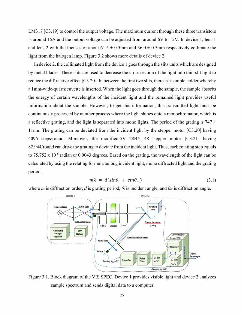
25
LM317 [C3.19] to control the output voltage. The maximum current through these three transistors
is around 15A and the output voltage can be adjusted from around 6V to 12V. In device 1, lens 1
and lens 2 with the focuses of about 61.5 ± 0.5mm and 36.0 ± 0.5mm respectively collimate the
light from the halogen lamp. Figure 3.2 shows more details of device 2.
In device 2, the collimated light from the device 1 goes through the slits units which are designed
by metal blades. These slits are used to decrease the cross section of the light into thin-slit light to
reduce the diffractive effect [C3.20]. In between the first two slits, there is a sample holder whereby
a 1mm-wide-quartz cuvette is inserted. When the light goes through the sample, the sample absorbs
the energy of certain wavelengths of the incident light and the remained light provides useful
information about the sample. However, to get this information, this transmitted light must be
continuously processed by another process where the light shines onto a monochromator, which is
a reflective grating, and the light is separated into mono lights. The period of the grating is 747 ±
11nm. The grating can be deviated from the incident light by the stepper motor [C3.20] having
4096 steps/round. Moreover, the modified-5V 28BYJ-48 stepper motor [C3.21] having
82,944/round can drive the grating to deviate from the incident light. Thus, each rotating step equals
to 75.752 x 10⁻⁶ radian or 0.0043 degrees. Based on the grating, the wavelength of the light can be
calculated by using the relating formula among incident light, mono diffracted light and the grating
period:
𝑚𝜆 𝑑 𝑠𝑖𝑛𝜃 𝑠𝑖𝑛𝜃 (3.1)
where m is diffraction order, d is grating period, θi is incident angle, and θm is diffraction angle.
Figure 3.1. Block diagram of the VIS SPEC. Device 1 provides visible light and device 2 analyzes
sample spectrum and sends digital data to a computer.

26
The mono lights are then directed to sensor 2 which is a photodiode, BPW-34, the diode is used
to measure the intensity of the mono lights. Signal from sensor 2 is then properly amplified and
filtered by the amplifier and the two low pass filters before collected, processed and filtered again
to eliminate noise by the 24-bit ADC and the Atmel328P microcontroller [C3.22]. From Figure
3.1, the signals from sensor 1 and sensor 2 after amplified and filtered by the electronic circuits are
sent to ADCs and the digital signals then enter the microcontroller.
Now the details of the error correction mechanism are presented. Basically, the light-source
monitoring sensor 1 collects the light-source intensity data, x, and the spectral sensor 2 records
spectral data, y, to send to the microcontroller for further processing. In case, the light-source
intensity is stable, there are no errors for both x and y. Therefore, x = 𝑥 , and y = 𝑦 , where
𝑥 and 𝑦 are the real value of x and y respectively. If the light intensity is unstable, then 𝑥
𝑥 , and 𝑦 𝑦 . The difference of these values can be defined as error values, and:
dx = 𝑥 𝑥 ; dy = 𝑦 𝑦 (3.2)
From experiment, when the light intensity is decreased, the spectral intensity is also decreased;
and, inversely, when the light intensity is increased, the spectral intensity is also increased.
Therefore, y is proportional with x.
Figure 3.2. Device 2 components: (a) light entrance, (b), (d) slits on the two sides of each unit, (c) sensor 1, (e) grating and its close view, (f) gears are used to increase the scanning steps, one gear is attached to the grating, (g) 5V regulator circuit supply energy for other electronics units inside the device 2, and the driver circuit using ULN2003 IC controls the stepper motor, (h) power supply input, (i) digital data output, (j) metal box protects inner circuits, (k) sensor housing, (l) amplifier circuits are combined two low-pass filters which filter out noise greater than 50Hz, (m) wall protects the sensor 2 area from the light entrance area, (n) sample cuvette.

27
Consequently, from equation (3.2), it can be seen that dy is proportional with dx, so dy ~ dx. Thus,
dy = f(dx), and:
Y= y + dy = y + f (𝑑𝑥) (3.3)
where Y is the corrected data, and f(dx) is considered as correction function. f can be proportional
with 𝑑𝑥, |𝑑𝑥| ∗ 𝑑𝑥|𝑑𝑥|, 𝑑𝑥 , …, or |𝑑𝑥| / ∗ 𝑑𝑥
|𝑑𝑥|, 𝑑𝑥 / , .... Because the form of f is not
known yet, let assume:
𝑓 𝑑𝑥 𝐶 ∗ 𝑑𝑥 𝐶 ∗ |𝑑𝑥| ∗ 𝑑𝑥|𝑑𝑥| 𝐶 ∗ 𝑑𝑥 ⋯ 𝐶 ∗ |𝑑𝑥| / ∗ 𝑑𝑥
|𝑑𝑥| 𝐶 ∗
𝑑𝑥 / ⋯ (3.4)
where, 𝐶 , 𝐶 , 𝐶 ,…, 𝐶 , 𝐶 , …are proportional constant values which must be estimated by
simulation on MATLAB software to have optimal coefficients. 𝑑𝑥|𝑑𝑥| has only two values, -1 or
+1, and indicates dx is negative or positive. To support for a successful simulation, some algorithms
and technique are manipulated.
3.2.1. Greedy technique
The way to find out these constants’ values are simple. It is based on the greedy technique
[C3.23] in which equation (3.4) is used in the simulation. At first, all 𝐶 , 𝐶 , 𝐶 ,…, 𝐶 , 𝐶 , … are
set to zero. Then, ∆𝐶 , ∆𝐶 , ∆𝐶 ,…, ∆𝐶 , ∆𝐶 , … are the increment values of 𝐶 , 𝐶 , 𝐶 ,…, 𝐶 , 𝐶 ,
… respectively, and set to certain small values. With the greedy technique, the simulation program
will start to find a certain proportional constant. Let’s start with 𝐶 . The program will add ∆𝐶 into
𝐶 , then substitute 𝐶 into equation (3.4) to calculate dy = f(dx). After that, put dy into equation
(3.3) to have the corrected data, Y, and then compare Y with 𝑦 to see whether Y is good or not.
Theoretically, Y is good when Y equals to 𝑦 . However, it is impossible, when there are many
other factors such as circuit noise can influence to the estimation process. Thus, to know when the
proportional estimation process should stop, some criteria such as absolute error (AR), relative
error (RE), error (ERR), least square (LS), or correlation parameter (CP) [C3.14] have been
applied, where the definitions of AE, RE, ERR, or LS are:
AE =∑ |𝑌 𝑖 𝑦 𝑖 |; RE =∑ |𝑌 𝑖 𝑦_𝑟𝑒𝑎𝑙 𝑖 | ⁄ 𝑦_𝑟𝑒𝑎𝑙 ;
ERR = ∑ 𝑌 𝑖 𝑦 𝑖 ; LS = ∑ 𝑌 𝑖 𝑦 𝑖 (3.5)

28
where i is the index of data vector Y and 𝑦 , and N is the number of data points, as Y and 𝑦
are discrete data. Let’s take AE for instance, after estimate the AE, a prior AE is compared with a
posterior AE. If a posterior AE < a prior AE, then the estimation of 𝐶 still need to be processed
again by adding it with ∆𝐶 . Inversely, the program will stop to search for 𝐶 and move to another
proportion constant. This process keeps going until all 𝐶 , 𝐶 , 𝐶 ,…, 𝐶 , 𝐶 , … are found to fulfill
f.
The advantage of the greedy technique is feasible to apply, but the disadvantage is that the
solution, f, and its correction coefficients results from the simulation program, is probably not the
best one. For example, with a certain suggested f, if the order of searching the correction
coefficients for f is 𝐶 , 𝐶 , 𝐶 ,…, 𝐶 , 𝐶 , … respectively, then the result is supposedly 𝑓 . Again,
changing the order of searching into 𝐶 , 𝐶 , 𝐶 , …, 𝐶 , 𝐶 , …, one can get 𝑓 𝑓 . Thus, if n orders
of searching are conducted, there can be n different forms of f. To determine which f is the better
one, the above criteria are looked at. Consequently, among these forms there should be the best
one.
In practice, when the form of the correction function is long and complicated, then it is not
efficient to code in a microcontroller. Moreover, it also increases running time in the measurement
which may lead to further error. For example, the running time for a measurement of more than
five minutes raises dark noise [C3.11] and/or potential light-intensity error during that time.
Therefore, in practice, several cognitive short forms of f are proposed for the simulation program.
3.2.2. Divide and conquer algorithm
From experiment, the correction function found from the Greedy technique cannot effectively
and adequately corrects the range of the interested spectrum. To circumvent the difficulty, the
investigated range is divided into smaller subdomain. At each of these subdomains, there will be a
correction function and corresponding parameters to conquer it. This technique is called divide-
and-conquer algorithm [C3.24]. Therefore, data error of each subdomain will be mitigated by the
function. Supposedly, there are n sub ranges, and so, there are n correction functions. In the
operation program, the main data domain R is cut into twelve subdomains, Ri.
𝑅 , 𝑅 , … , 𝑅 , 𝑅 𝑅 𝑅 ⋃ 𝑅 ⋃ … ⋃ 𝑅 ⋃ 𝑅 𝑅
(3.6)

29
Theoretically, the smaller the sub ranges are divided, the better the corrected data are. However,
when the number of the sub ranges increases, the time which is used to process data will be longer.
There must be a balance among measuring time, the number of sub ranges, and the measured data.
In this work, through experiments, twelve sub ranges are formed to perform the data correction
task. As mentioned above, to achieve the best results, MATLAB simulation will be used to search
for them. In the MATLAB code, some sub recursive functions are built and recalled continuously
in the simulation. In general, the problem is just shrinking into smaller domains to get better
simulation results which serve for the later steps.
3.2.3. Kalman algorithm
There is one more obstacle still able to intervene the searching of best 𝐶 , 𝐶 , 𝐶 ,…, 𝐶 , 𝐶 , ….
In practice, after running the searching simulation with the raw data x, to get f, and applying it to
correct the spectral data, the results are not satisfied as expect. Since, when the raw light-source-
monitoring data, x, which could have noises [C3.11, C3.12, C3.13], quantization error [C3.14], and
unstable light-intensity error, are sent to f, not only is the unstable light-intensity error transformed
by f but also by the mixture of noises and quantization error. These noises and quantization error
will make the operating criteria (AE, RE, ERR, LS, or CP) work ineffectively and inadequately.
Consequently, x must be treated by certain approaches before use.
Moreover, the chosen approach should be applicable and feasible for the microcontroller code
and satisfies real-time application without any processing lag and procrastination. For feasibility,
two outstanding there are algorithms moving average [C3.14] and Kalman algorithm [C3.23,
C3.25, C3.26]. For real-time applications, Kalman algorithm has been proved by some simple
experiments that dominates the moving average algorithm. After being treated by the Kalman
algorithm, ideally, dx (dx = 𝑥 𝑥 ) containing only unstable light-intensity error, which is
useful information, will be ready to serve for the correction process.
Details of the Kalman algorithm can be found in [C3.23, C3.25, C3.26], it is necessary to focus
on some equations and quantities of the theory for later applying explanation. First, the system is
supposed to be linear [C3.26, C3.27], so its state equation has the form of:
𝑿𝒌 𝑨𝒌𝑿𝒌 𝟏 𝑩𝒌𝑼𝒌 𝑾𝒌 (3.7)
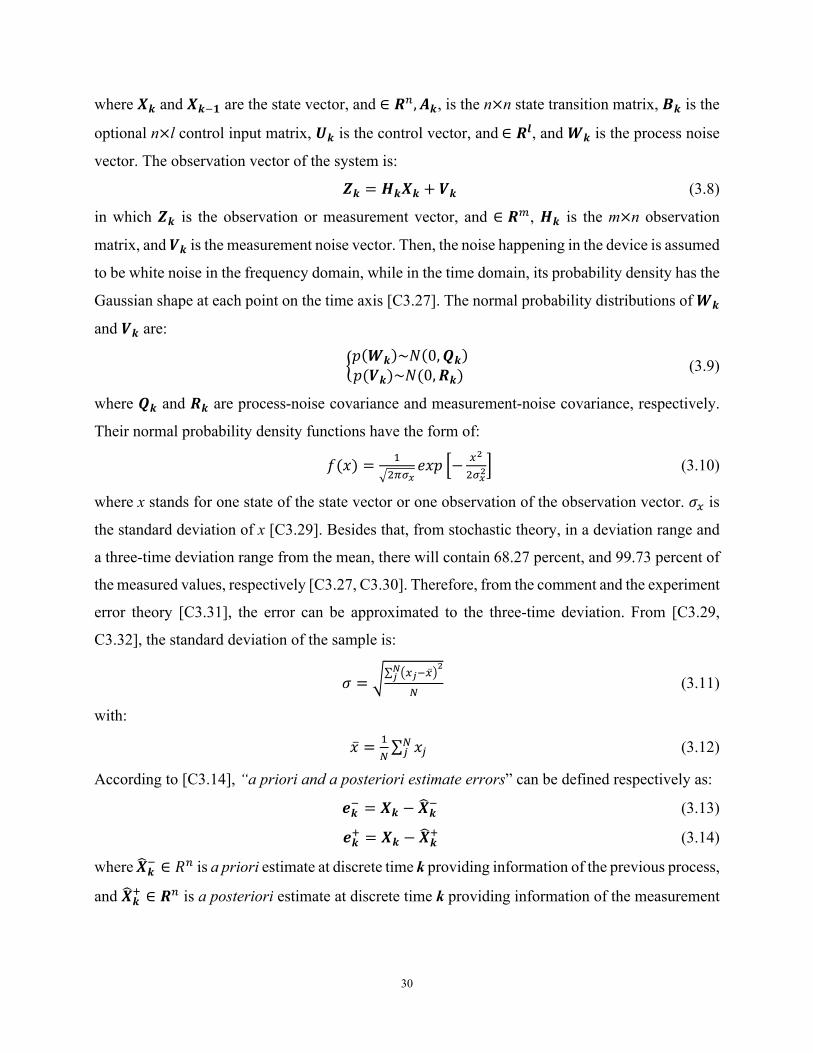
30
where 𝑿𝒌 and 𝑿𝒌 𝟏 are the state vector, and ∈ 𝑹 , 𝑨𝒌, is the n n state transition matrix, 𝑩𝒌 is the
optional n l control input matrix, 𝑼𝒌 is the control vector, and ∈ 𝑹𝒍, and 𝑾𝒌 is the process noise
vector. The observation vector of the system is:
𝒁𝒌 𝑯𝒌𝑿𝒌 𝑽𝒌 (3.8)
in which 𝒁𝒌 is the observation or measurement vector, and ∈ 𝑹 , 𝑯𝒌 is the m n observation
matrix, and 𝑽𝒌 is the measurement noise vector. Then, the noise happening in the device is assumed
to be white noise in the frequency domain, while in the time domain, its probability density has the
Gaussian shape at each point on the time axis [C3.27]. The normal probability distributions of 𝑾𝒌
and 𝑽𝒌 are:
𝑝 𝑾𝒌 ~𝑁 0, 𝑸𝒌𝑝 𝑽𝒌 ~𝑁 0, 𝑹𝒌
(3.9)
where 𝑸𝒌 and 𝑹𝒌 are process-noise covariance and measurement-noise covariance, respectively.
Their normal probability density functions have the form of:
𝑓 𝑥 𝑒𝑥𝑝 (3.10)
where x stands for one state of the state vector or one observation of the observation vector. 𝜎 is
the standard deviation of x [C3.29]. Besides that, from stochastic theory, in a deviation range and
a three-time deviation range from the mean, there will contain 68.27 percent, and 99.73 percent of
the measured values, respectively [C3.27, C3.30]. Therefore, from the comment and the experiment
error theory [C3.31], the error can be approximated to the three-time deviation. From [C3.29,
C3.32], the standard deviation of the sample is:
𝜎∑ ̅
(3.11)
with:
�̅� ∑ 𝑥 (3.12)
According to [C3.14], “a priori and a posteriori estimate errors” can be defined respectively as:
𝒆𝒌 𝑿𝒌 𝑿𝒌 (3.13)
𝒆𝒌 𝑿𝒌 𝑿𝒌 (3.14)
where 𝑿𝒌 ∈ 𝑅 is a priori estimate at discrete time k providing information of the previous process,
and 𝑿𝒌 ∈ 𝑹 is a posteriori estimate at discrete time k providing information of the measurement

31
𝒁𝒌. From (3.13) and (3.14), the covariance of a priori error and the covariance of a posteriori error
are respectively:
𝑷𝒌 =E[𝒆𝒌 𝒆𝒌𝑻] (3.15)
𝑷𝒌 =E[𝒆𝒌 𝒆𝒌𝑻] (3.16)
A posteriori estimate has the form [C3.11, C3.12, C3.14] of:
𝑿𝒌 =𝑿𝒌 𝑲𝒌 𝒁𝒌 𝑯𝒌𝑿𝒌 =(1-𝑲𝒌𝑯𝒌) 𝑿𝒌 +𝑲𝒌𝒁𝒌 (3.17)
where 𝒁𝒌 𝑯𝒌𝑿𝒌 ) is the residual or measurement innovation which shows the difference
between the measurement and a priori estimate, and 𝐾 , named Kalman gain or blending factor, is
chosen by minimizing the covariance in (3.16). From [C3.26, C3.27, C3.32], 𝑲𝒌 is:
𝑲𝒌 𝑷𝒌 𝑯𝒌𝑻 𝑯𝒌𝑷𝒌 𝑯𝒌
𝑻 𝑹𝒌 (3.18)
From (3.18), when the measurement noise covariance is small, 𝒁𝒌 has high fidelity and Kalman
gain will be large. At that time, from (3.17), the weight coefficient of 𝒁𝒌 is greater than the weight
of 𝑿𝒌 , so 𝑿𝒌 will “believe” more in 𝒁𝒌 than 𝑿𝒌 . Inversely, as 𝑷𝒌 is small, Kalman gain will be
small and 𝑿𝒌 will “believe” more in 𝑿𝒌 than 𝒁𝒌. Figure 3.3 shows the operation loop of Kalman
algorithm.
Figure 3.3. Kalman filter operation loop
In practice, 𝑸𝒌 and 𝑹𝒌 can be estimated before applying the Kalman filter. In the study, 𝑹𝒌 is
calculated by several rough measured data, but 𝑸 is determined by MATLAB simulation to get
the best results. These values, during operation, can be constant, so be presented without discrete-
time subscript k. From [C3.23, C3.25, C3.26], one can see that 𝑹𝒌= 𝜎 . In practice, 𝑹𝒌 is easily
determined by using equation (3.11) and equation (3.12).

32
3.2.4. Performance description
In this section, all the processes manipulated to process data with the order of correction
function, process noise covariance, and correction coefficients findings, by MATLAB simulation
are presented.
First, in equations (3.1), (3.2), and (3.4), the values of real data of sensor 1 and sensor 2 were
mentioned and known. However, that is only a hypothesis to help establish the processing
algorithm. In practice, the values measured in stable conditions are considered approximately equal
to the real values and are reference values to serve for comparison and calculation in simulation.
The flowchart in Figure 3.4 shows the core algorithm for simulation program, where 𝒀 and 𝒀
are spectral data measured in unsteady conditions and good conditions respectively, whereas 𝑿
and 𝑿 are light intensity data recorded in these two cases. Conventionally, 𝑿 and 𝒀 are data
with unstable-light-intensity data with error, and 𝑿 and 𝒀 are reference data.
Second, noticing that 𝒀 and 𝒀 are 24-bit data, while 𝑿 and 𝑿 are 10-bit data. Then, 𝑸𝟏, 𝑒 ,
and ∆𝑸, respectively are process noise covariance, measurement error, and the decrement of 𝑸𝟏
sequentially. Especially, 𝑒 takes two roles, a posterior error and a priori error in the Kalman
module. Many data, 𝑿 , 𝑿 , 𝒀 , and 𝒀 , were measured and saved in datasets before the
simulations. 𝐿𝑆 and 𝐿𝑆 are the least square parameters which are used to operate the
loop. 𝑏 , 𝑏 , …, and 𝑏 which are the fixed values are set to satisfy the condition:
0<𝑏 <𝑏 <…<𝑏 <𝒀 (3.19),
and they are considered as “boundary” values to help divide the grand spectral data domain into
subdomains. In the simulation program, the maximum potential number of the subdomains which
are non-empty is 12, if the minimum data value is smaller than 𝑏 , the maximum data value is
greater than 𝑏 , and at any range of (0, 𝑏 ), [𝑏 , 𝑏 ), …, [𝑏 , 𝑏 ), [𝑏 , 𝒀 both positive and
negative dX values exist. 𝐶 , 𝐶 , …, 𝐶 are the correction parameters, whereas dC is the increment
of these parameters.
3.2.4.1 Correction function finding
As discussed above, to make the correction function feasible and applicable, several short forms
of equation (3.4) are proposed. They are sequentially replaced into the simulation program which
is illustrated by the flowchart in Figure 3.4. Thus, the simulation program will help to find the

33
correction coefficients for the suggested functions. After finishing each simulation, the program
will return not merely 𝑸𝟏, 𝐶 , 𝐶 , …, 𝐶 , but also AE, ERR, LS, or CP which can be used as the
quality assessment criteria of the correction functions. Therefore, which correction function with
the prominent assessment parameters is to be adopted. The simulation program starts by loading
data 𝑿 , 𝑿 , 𝒀 , and 𝒀 from the assigned datasets and initiating the values for 𝑸𝟏, 𝑒 , 𝑒 , ∆𝑸,
𝐿𝑆 , 𝐿𝑆 , 𝑏 , 𝑏 , …, 𝑏 , and dC.
In the flowchart, 𝑿 and 𝑿 are processed by the Kalman algorithm to mitigate the quantization
error and electronic noises, which may remain, albeit being filtered by hardware filters, to keep the
light-source-intensity information as clean as possible. The searching simulation is not successful
if the light-source data still have high quantization error and noises. Furthermore, to empower the
corrector to work effectively and adequately, the data from sensor 1 and sensor 2 should be
collected by applying unstable-light-intensity styles from gradual to fast changes and from mono-
changing, to multi-changing styles with large enough fluctuation amplitudes to use in the
simulation. However, at this stage, the correction coefficients of the correction function are the
priority, so 𝑸𝟏 is cognitively set to a certain value that is good enough for the simulation and of
course, larger than 𝑄 . ∆𝑸 is set to zero to not influence on 𝑸𝟏.
Let’s look at the operation in the flowchart of Figure 3.4. At first, 𝐿𝑆 = 0 < 𝐿𝑆 = 1
and 𝑸𝟏 > 𝑄 satisfy the main condition in the flowchart. Then, 𝑸𝟏 is decreased by a ∆𝑸 = 0, so
it does not change. 𝑿 and 𝑿 are smoothed by the Kalman module that returns 𝑿 and 𝑿
respectively prior to calculate dX = 𝑿 𝑿 . Then, the Division function is called to divide 𝒅𝑿,
𝒀 , and 𝒀 into smaller domains. At this point, the divide-and-conquer algorithm is applied to
separate the grand data domain into smaller domains which are more easily to conquer and to find
the solution. The way to divide the data is illustrated in the flowchart of Figure 3.5.
In this function, there are thirteen indexes, i, j, k, l, m, n, o, r, s, t, u, v, w to address data points
in the vector 𝒅𝑿, 𝒀 , and 𝒀 . Initially, i is smaller than the number of data elements of 𝒀 that is
checked by the first condition in Figure 3.5. i is increased one unit and the condition of whether
𝒅𝑿(i) is positive is checked. With either “Yes” or “No” this first data element, 𝒀 is compared with
𝑏 , 𝑏 , 𝑏 , 𝑏 , and 𝑏 to see to which data subdomain it must belong to. The difference here is that
if 𝒅𝑿(i) > 0, the first six subdomains, 𝑌 , , 𝑌 , , …, 𝑌 , for 𝒀 , 𝑌 , , 𝑌 , , …, 𝑌 , for 𝒀 , 𝒅𝑿 , ,
𝒅𝑿 , , …, 𝒅𝑿 , of 𝒅𝑿, are used for the arrangement. In case 𝑑𝑋(i) < 0, the second six subdomains,
𝑌 , , 𝑌 , , …, 𝑌 , for 𝒀 , 𝑌 , , 𝑌 , , …, 𝑌 , for 𝒀 , 𝒅𝑿 , , 𝒅𝑿 , , …, 𝒅𝑿 , of 𝒅𝑿, are used for the

34
assembly. When 𝒅𝑿(i) = 0, the running point will jump back to the first condition. Then, the same
procedure is repeated until i, loop index, is larger than the number of the data elements of 𝒀 .
Especially, when all vector 𝒅𝑿 = 0, the division will return twelve empty subdomains. In this case,
there is no need to fix spectral data. When all 𝒅𝑿 > 0, from Figure 3.5, the left side condition boxes
will be conducted. Consequently, the first six subdomains are none-empty, and the second six
subdomains are empty. Inversely, when all 𝒅𝑿 < 0, the second six subdomains are none-empty,
and the first six subdomains are empty.
Figure 3.4. The simulation flowchart to find correction parameters or process noise covariance 𝑸𝟏.
Again, from Figure 3.4, after receiving the returned twelve data subdomains, the main
simulation program will call the Finding function to find the correction coefficients. The
simulation initiates index i from 1 to 12 to access data in the subdomains. The algorithm of this
module is shown in Figure 3.6. The data subdomain of order i, 𝑌 , , 𝑌 , , 𝑑𝑋 , are loaded. In this
process, 𝑙𝑠 and 𝑙𝑠 are also the least square values to serve for operating the loop. When

35
𝑙𝑠 < 𝑙𝑠 and 𝑌 , is different from null, 𝐶 is increased by a dC. 𝑙𝑠 < 𝑙𝑠 condition
means the currently corrected sub-data is better the previous corrected data, so this sub-data still
can be better amended. Then, the suggested correction function is applied to fix 𝑌 , and returns
𝑌 , . Next, the subprogram will call Assessment function to calculate LS, AE, ERR based on
equation (3.5), the corrected data, 𝑌 , , and reference data, 𝑌 , , and updates 𝑙𝑠 with 𝑙𝑠 ,
and 𝑙𝑠 with LS. Then, the subprogram keeps going back to the operating condition until
𝑙𝑠 > 𝑙𝑠 which means the current corrected data cannot be further corrected. From the
flowchart in Figure 3.4, the finding module is called twelve times to access all the subdomains
without noting of whether they are null or not.
Figure 3.5. The diagram is presented for Division function.
After escaping from the finding module and having all correction coefficients, the main
simulation program will apply these values to correct all the sub data, 𝑌 , , 𝑌 , , …, 𝑌 , , of the
grand spectral data, 𝒀 by calling the Correction function which is built from the suggested
correction function, f. The equation is in the form:

36
𝑌 , (j) = 𝑌 , (j)+ 𝐶 *f[(𝑑𝑋 (j), 𝑌 , (j)] (3.20)
Then, the Assessment will help to evaluate LS, ERR, AE, or CP by using 𝒀 and 𝒀 . Thus, it is
similar to the above description of how the least square criterion works that the program will not
stop when 𝐿𝑆 < 𝐿𝑆 ….
Finally, in the end, the simulation will return many coefficients, but the most interesting
coefficients are LS, ERR, AR, and CP. Therefore, with each suggested short-form correction
function, there are the most interesting coefficients. Assessing these coefficients, the best one is
chosen to be used in the correction function.
Figure 3.6. The Finding flowchart for correction parameters
3.2.4.2. Process noise covariance finding
After finding the appropriate correction function from the suggested functions, the simulation
program is applied again to find the process noise covariance, 𝑸 . Although, 𝑸 used above is good
enough, it may not be the best to assure the light-source-intensity data as clean as possible. As
mentioned above, many types of data will be used to serve the simulation. Currently, ∆𝑸 is
cognitively set to a certain value which is small enough for the searching simulation. The procedure
exactly repeats what is described in section 2.4.1, except for the main operating condition must
account for the condition 𝑸 𝑄 , and at every loop, 𝑸 is decreased by a ∆𝑸. When the
condition 𝐿𝑆 < 𝐿𝑆 and 𝑸 𝑄 cannot be satisfied, the simulation program will cease

37
to return 𝑸 . This value of process noise covariance is to be expected that can keep the best light-
source data from the noise.
3.2.4.3. Correction coefficients finding
After the above crucial steps, the main simulation program, which having the flowchart depicted
in Figure 3.4, simply reinstalls the found correction function and 𝑸 back into itself to find 𝐶 , 𝐶 ,
…, 𝐶 . Before that, ∆𝑸 is set to zero. At the end, it returns correction coefficients.
3.2.4.4. Application
After the simulation step, all necessary key components, correction function, correction
coefficients, and process noise covariance are provided and ready to apply in the device and to
build the Kalman corrector. Figure 3.7 illustrates the procedure of collecting and processing data.
The light intensity signal from sensor 1 enters the 10-bit ADC and the spectral intensity signal from
sensor 2 goes to the 24-bit ADC.
Figure 3.7. The main roles of Kalman algorithm and their correlation with other parts
These signals are digitalized to become digital data. X is filtered out noises and quantization error
by 𝑸𝟏 to become 𝑿. Next, the compare block will calculate dX which 𝒅𝑿 𝑿𝒐 𝑿, where 𝑿 is
a loosely optional value. 𝑿𝒐 can be equal to a certain standard value or a measured value which is
measured ahead before any spectral measurement. Then, dX and Y values will be delivered by the
subdomain deliver to assigned data subdomains which are characterized by 𝑏 , 𝑏 , …, 𝑏 and
controlled by dX. Here, the subdomain deliver works similar to the division. It will base on whether
dX is positive or negative and to what range among (0, 𝑏 ), [𝑏 , 𝑏 ), …, [𝑏 , 𝑏 ), [𝑏 , 𝒀 Y
belongs to. Y is then sent to the correction function which is governing the data subdomain
corresponding with that range (section 2.4.1 and Figure 3.6). For example, if dX > 0, and 0 < Y <
𝑏 , then Y is sent to the corresponding subdomain, where is governed by a data correction function
38
of 𝒀 founded by the previous simulation, to be thoroughly amended. This is performed in real
time, so dX and Y are no longer data vector but rather discrete-time data measured at each discrete
time.
3.3. Results
The light source in this study is visible, its spectrum is from 450nm to 750nm. For convenience
in the following figures, on the vertical axis, the unit for the light intensity or spectra is an arbitrary
unit (a.u). With the spectral intensity plot, the horizontal axis presents the step unit corresponding
to the scanning steps of the stepper motor instead of wavelength unit or number wavelength unit
which can be changed among them by using equation (3.1). The step value is changed to rotation
angle and the angle is translated into wavelength. However, in the light-source intensity plots, the
step value on the horizontal axis simply corresponds to the discrete time values in the sampling
signal.
As described earlier, light intensity may increase or decrease randomly when the voltage
regulator is not working well or changes due to other reasons such as physical conditions, ambient
air temperature, lamp temperature, or warm up and working time. The changes can also be in mono
trend by some conditions such as the drift of the battery. Before running the simulation program,
many experimental data have been recorded to serve the simulations. The recorded data are
collected under the un-change and slightly change working conditions to simulate the unstable
factors as mentioned in the introduction which can lead to the slightly change in light intensity.
Then data recorded in well working conditions (external stable power supply) serve as reference
data for the assessment process.
3.3.1. Initial 𝑸𝟏 selection for simulation
In Figure 3.8, the red-dot line is the recorded raw 10-bit data of the light intensity source which
was slightly adjusted to simulate unstable light source. Several values of 𝑸𝟏 are tested to study the
features of 𝑸𝟏. One may see that the smaller the 𝑸𝟏 is, the smoother output data from the Kalman
function will be. This leads to that 𝑿𝟏, the blue line, is so smooth, when 𝑸𝟏 is so small, for example
𝑸𝟏 10 (it is matching with this type of data and measurement error). Thus, not only the

39
electronics noises and quantization error are removed but also some useful and crucial information
from the light source. Obviously, this will ruin the process of the data correction and simulation.
Figure 3.8. Raw intensity data and its filtered data with different 𝑸𝟏 values.
When 𝑸𝟏 10 , the filtered data, 𝑿 , plot is the cyan line. Currently, 𝑿 keeps much light-
intensity information, but also some electronic noises and quantization error as well. If using this
filtered data for simulation, the results, such as correction coefficients, or corrected spectral data,
may not be the best.
Therefore, neither too large nor too small 𝑄 can lead to good results which are demonstrated
by plot groups of Figure 3.9. (a), and Figure 3.9. (b), respectively. In both cases, the corrected data
are not close to or similar to the reference. Section 2.4.2 shows how to obtain an appropriate and
adequate 𝑄 . To serve for the simulation of finding correction function which will be discussed in
the next section, 𝑄 is set to 10-3.
3.3.2. Correction function choice
A multi-changing data set 1 is loaded for test. The general initial values are: b = 7*105, b1 = b,
b2 = 2*b, b3 = 3*b, b4 = 3.6*b, b5 = 4*b, 𝑸𝟏 = 10-3, 𝑒 𝑒 1, and 𝑒 𝑒 500
(experimentally determined by equation (3.11) and equation (3.12)). With each correction function
which is chosen, the increment, dC, of the correction parameters must be cognitively adjusted to a
certain appropriate value that assures that the finding function will be called at least several times.
This value should not be so small because the simulation process may last too long without better
results. In the next section, four typical correction functions are investigated to select the most
appropriate one in these. These proposed functions are based on experiment, evaluation, and
observation of the results to adjust logically. Objectively, these correction functions are tested with
(a.u
.)

40
the same dataset 1. Notice that, LS, AE, ERR, and CP are the controlling criteria that are also used
as effective and qualitative parameters for the decision.
Figure 3.9. Results of measurement data and processed data (a) the three plots of data in the case of 𝑄1=0.9, and (b) the three plots of data in case of 𝑄1≈1.27*10 .
In Table 3.1 below, in Table 3.1 below, 𝑓 , 𝑓 , 𝑓 , and 𝑓 are short correction function forms.
The formulas of these functions are in Appendix A.
Table 3.1. LS, AE, ERR, and CP of 𝑓 , 𝑓 , 𝑓 , and 𝑓 are shown respectively.
LS AE ERR CP(𝒀𝟏, 𝒀𝟐) CP(𝒀𝟏, 𝒀𝟐) Feasibility
𝑓 2.159*1011 1.483*10 2.773*106 0.999608 0.999968 Medium
𝑓 1.846*1011 1.3747*10 3.3367*106 0.999608 0.9999769 Low
𝑓 1.9372*1011 2.3045*10 3.3367*106 0.999608 0.9999725 Low
𝑓 1.840*1011 1.3719*10 2.8859*106 0.999608 0.9999756 High
The LS, AE, and ERR are expected as small as possible, i.e., the corrected spectral data are
similar to the reference spectral data. For CP, if the two signals of the data are very close to each
other, CP will be approximate to one. In the table, an auxiliary index is the feasibility. Simply, it
takes the values of relative evaluation which is based on the form of the correction function. If this
(a.u
.)
(a.u
.)
(a.u
.)
(a.u
.)
(a) (b)

41
index is high, the function is easily applied. In some cases, this index can strengthen a decision,
albeit merely auxiliary one. In the table, the prominent values are highlighted. Observing Table
3.1, one possibly sees the most outstanding correction function is 𝑓 , and the second one is 𝑓 ,
finally, 𝑓 is selected.
3.3.3. Process noise covariance search
After the correction function, 𝒀𝟏,𝒊(j) = 𝒀𝟏,𝒊(j) + 𝑪𝒊*𝒅𝑿𝒊(j)* 𝒀𝟏,𝒊 𝒋 , has been chosen, the process
noise covariance, 𝑸𝟏, search is the next step. As previously discussed, to achieve an appropriate
and adequate of 𝑸𝟏, many datasets which were measured under different light-intensity-changing
styles are used. The multi-changing dataset 2 to dataset 19 (named by the authors) are chosen to
be loaded into the simulation program. Table 3.2 provides the values of 𝑸𝟏 gathered after the
simulations.
Table 3.2. 𝑸𝟏 values of multi-changing datasets
dataset
2
dataset
3
dataset
4
dataset
5
dataset
6
dataset
7
dataset
8
dataset
9
dataset
10
𝑸𝟏 0.0071 0.0321 0.0561 0.0147 0.0112 0.0076 0.0352 0.0119 0.0155
dataset
11
dataset
12
dataset
13
dataset
14
dataset
15
dataset
16
dataset
17
dataset
18
dataset
19
𝑸𝟏 0.0144 0.0349 0.0124 0.0203 0.0126 0.0249 0.0107 0.0165 0.0268
From the above 𝑸𝟏 search simulations corresponding with multi-changing data sets, a 𝑸𝟏 will
be chosen. There will be some points of view in choosing 𝑸𝟏. For instance, one may suppose that
the average 𝑸𝟏 partly satisfies all the cases of light intensity change or the greatest 𝑸𝟏 of the found
values is the safe solution as the Kalman filter can catch up the possibly fastest and, obviously,
slowest intensity change of the studied data sets. However, with the later philosophy, 𝑸𝟏,𝒎𝒂𝒙 will
be greater than the average one, 𝑸𝟏, and then the corrected data pertaining to 𝑸𝟏,𝒎𝒂𝒙 is probably
not as smooth as the corrected data of 𝑸𝟏. If 𝑸𝟏,𝒎𝒊𝒏 is selected, there will probably be some quick-
changing-light intensity not detected well by the Kalman. To implement in the device, the selected
process noise covariance is 𝑸𝟏 = 0.0203. After selecting the best correction function and the

42
appropriate 𝑸𝟏 for the Kalman module, the next process is to load the mono-changing data sets to
find the correction parameters, Ci.
3.3.4. Correction parameters finding
In this section, the mono-changing datasets are viewed. In these datasets, there are two subtype
data where one has spectral and light intensity data greater than the reference spectral and light
intensity data, and the other one has spectral and light intensity data smaller than the reference
spectral and light intensity data. Thus, with these types of the dataset, after division module is
called, there should be six continuous empty data subdomains and six continuous non-empty data
subdomains. The upper-subdomain data and lower-subdomain data are investigated separately to
find the correction parameters. The full tables of the correction parameters are attached in
Appendix B. Table 3.3 and Table 3.4 provide short results of the tables.
Table 3.3. Ci values of upper-subdomain data.
Data set 𝐶 𝐶 𝐶 𝐶 𝐶 𝐶 𝒅𝑿
1 0.00386 0.00264 0.00245 0.00233 0.00208 0.00207 5.7078
… … … … … … … …
30 0.00396 0.00254 0.00222 0.00229 0.00216 0.00211 28.5594
Table 3.4. Ci values of lower-subdomain data.
Data set 𝐶 𝐶 𝐶 𝐶 𝐶 𝐶 𝒅𝑿
1 0.00355 0.00231 0.00219 0.00187 0.0019 0.00188 -20.2399
… … … … … … … …
30 0.00347 0.00239 0.00215 0.0021 0.00197 0.00198 -29.5559
Average 0.00351 0.00239 0.00210 0.00206 0.00201 0.00197
Notice that dX is adjusted from around the range of -40 to 30 units corresponding to the potential
change of the light intensity. Each unit corresponds to approximately 4.9mV difference when the
10-bit ADC of the microcontroller is used. For a small change in light intensity, the relationship of
dX and Ci is expected to be linear with that the best applied correction function, 𝑌 , (j) = 𝑌 , (j)
+ 𝐶 *𝑑𝑋 (j)* 𝑌 , 𝑗 . When dX is adjusted to different positive and negative values which
correspond to the simulations of different voltage increases and decreases, one can see from the

43
C1 = 0.00369 C2 = 0.00256
C4 = 0.00233 C6 = 0.00219
C3 = 0.00227
C5 = 0.00222
C8 = 0.00239 C9 = 0.002103 C7 = 0.00351
C10 = 0.00206 C11 = 0.00201 C12 = 0.00197
plots of Figure 3.10 and Figure 3.11 that Ci and dX relationship is linear as expected and the slope
angle is zero. In this case, one can take the mean values of Ci to make it as the correction
coefficients of the corresponding subdomains.
3.3.5. Practice
Through experiments and simulations, the correction function below is used:
𝑌 , (j) = 𝑌 , (j) + 𝐶 *𝑑𝑋 (j)* 𝑌 , 𝑗 ,
and the noise process covariance, 𝑄 = 0.0203, and the correction coefficients, C1 = 0.003709, C2
= 0.002577, C3 = 0.002278, C4 = 0.002368, C5 = 0.002242, C6 = 0.002215, C7 = 0.003694, C8 =
0.002449, C9 = 0.002103, C10 = 0.002155, C11 = 0.002084, C12 = 0.002036, have been found
through the simulation described in the previous sections.
Figure 3. 10. The plots of correction coefficients and dX of upper-subdomain data
Figure 3.11. The plots of the correction coefficients and dX of lower-subdomain data

44
3.3.5.1. Dataset correction simulation
Now with the all the parameters and function found, one can check to see how the output data
from the corrector is better than the uncorrected data. For the process assessment, two new
quantities are added:
|𝒅𝒀𝟏| |𝒀𝟐 – 𝒀𝟏| (3.21)
|𝒅𝒀𝟐| |𝒀𝟐 – 𝒀𝟏| (3.22)
Equations (3.21) and (3.22) are the absolute errors of the uncorrected data and corrected data,
respectively. Figure 3.12 shows the plots of the new quantities, |𝒅𝒀𝟏|, |𝒅𝒀𝟐| of the multi-changing
data and mono-changing data of the two different styles datasets. The expectation here is that the
absolute error plots is as close to the zero line as possible. From the plots, the corrected data is
better than the uncorrected data. The intensity plots only illustrate how the light intensity was
changed to simulate possible reality situations.
Figure 3.12. (a): |𝑑𝑌 | and |𝑑𝑌 | plots of multi-changing dataset 24; (b): |𝑑𝑌 | and |𝑑𝑌 | plots of lower-mono-changing dataset 1
3.3.5.2. Measurements on air, H2O, and KMnO4 samples
After the simulation testing, the correction function and the parameters are applied into the
device for further test. For the test, the reference data are still required. The light intensity of the
light source is adjusted similarly when the data with error were recorded to serve for the above
simulations. The difference here is the data with error will be corrected immediately by the
(a) (b)
(a.u
)
(a.u
)

45
corrector module which is coded into the Atmel328P processor. To check the effectiveness and
ability of the corrector, several different types of samples are required (air, H2O, and KMnO4
samples) under the light intensity changes in both mono-changing and multi-changing strategies.
From experiment data, spectral data, light intensity data, and errors are plotted, Experimental
results prove that the corrector module works well as can be seen in Figure 3.13. Note that there
are four types of different samples and three types of plots in the figure to illustrate the work of
the corrector. The errors of the data after the correction are also plotted.
Figure 3.13. Experimental data of different samples. (d): 0.011g KMnO4 and 30ml distilled H2O; (b): air; (c): 0.021g KMnO4 and 25ml distilled H2O; (d): distilled H2O.
(a) (b)
(c) (d)

46
By defining the simple formula, r = |𝒅𝒀𝟏|
|𝒅𝒀𝟐| , indicates how many times the corrector reduces the
light-intensity error. According to calculation from the measured data, r 10 times. At some local
data points, it could reach to 60 to 70 times. This coefficient is a used as a merit to evaluate the
effectiveness of the Kalman corrector. However, it just shows much meaningful when there is
much light-intensity error happening, albeit a good coefficient.
3.4. Discussion and Conclusion
In general, the Kalman algorithm is modified as a corrector to compensate for the data error
caused by the unstable light source in a VIS SPEC. The single-beam-24-bit visible spectrometer,
which is empowered by an auxiliary photodiode sensor, an appropriate correction function, and
Kalman algorithm, can automatically correct the error caused by the light-source-intensity
instability which happens randomly or by drifting of the sources. In average, when there is error in
the spectral data, it can be reduced approximately by 10 times. The results show a good
performance both in simulations and experiments.
One drawback of the technique is the using of average of 𝑸𝟏,𝒎𝒊𝒏 to 𝑸𝟏,𝒎𝒂𝒙 from simulation.
Section 3.3 provides a range of the applicable values of the noise process covariance. For being
able to adapt to the diversity of light-intensity instability, the mean value of the range is selected.
Consequently, the data with error may not be perfectly corrected due to either the lack of or not
enough light-intensity error information and/or quantization errors still remaining in the light-
intensity data.
To improve the ability of the corrector module, other methods can be applied along with this
technique to achieve better results. For example, one can use moveable boundaries, instead of
applying the currently fixed boundaries. With moveable boundaries, LS, AE, ERR, and correlation
coefficient are still the operation criteria.
Appendix A
The short correction forms of the formulas used in section 3.2, Table 3.1:
𝑓 𝑌 , (j) + 𝐶 *𝑑𝑋 (j)*𝑌 , (j),
𝑓 𝑌 , (j) + 𝐶 *𝑑𝑋 (j)* 𝑌 , 𝑗 ,

47
𝑓 = 𝑌 , (j) + 𝐶 *𝑑𝑋 (j)* 𝑌 , 𝑗 ,
𝑓 = 𝑌 , (j) + 𝐶 *𝑑𝑋 (j)* 𝑌 , 𝑗 .
Noticing that the form of 𝑓 , 𝑓 , 𝑓 , and 𝑓 is slightly different from equation (3.4). As in the
experiments, authors found that the correction function work much more effectively if 𝑌 , 𝑗 is
inserted, where n is 1, 2, 3, …, or 1/2, 1/3, 3/2. Thus, there is a relation between the correction
function f with not only dX but also Y.
Appendix B
The values of Ci of the upper-subdomain and lower-domain data are collected by simulation and
used in section 3.4.
Table 3.3: Ci values of upper-subdomain data.
Data set
𝐶 𝐶 𝐶 𝐶 𝐶 𝐶 𝒅𝑿
1 0.00386 0.00264 0.00245 0.00233 0.00208 0.00207 5.7078
2 0.00345 0.00261 0.00202 0.00246 0.00231 0.00230 4.9686
3 0.00392 0.00240 0.00231 0.00231 0.00206 0.00206 4.4369
4 0.00377 0.00283 0.00204 0.00243 0.00240 0.00227 4.6495
5 0.00356 0.00238 0.00201 0.00248 0.00229 0.00226 10.3858
6 0.00359 0.00242 0.00196 0.00213 0.00206 0.00202 9.8095
7 0.00364 0.0026 0.00227 0.00230 0.00222 0.00216 9.8672
8 0.00328 0.00256 0.00247 0.00222 0.00212 0.00218 9.5766
9 0.00345 0.00264 0.00236 0.00233 0.00220 0.00230 8.5105
10 0.00391 0.00267 0.00238 0.00248 0.00229 0.00231 15.2758
11 0.00393 0.00272 0.00234 0.00225 0.00216 0.00213 14.6995
12 0.00380 0.00277 0.00238 0.00230 0.00224 0.00217 14.5844
13 0.00398 0.00272 0.00247 0.00224 0.00215 0.00210 14.0529
14 0.00391 0.00265 0.00215 0.00257 0.00238 0.00233 12.1743
15 0.00340 0.00249 0.00246 0.00232 0.00215 0.00219 12.7739
16 0.00341 0.00260 0.00236 0.00255 0.00236 0.00236 16.4325
17 0.00341 0.00265 0.00233 0.00234 0.00224 0.00219 15.8561
18 0.00357 0.00259 0.00242 0.00230 0.00215 0.00212 15.3245
19 0.00371 0.00274 0.00252 0.00240 0.00227 0.00224 16.5607
20 0.00342 0.00228 0.00210 0.00249 0.00234 0.00231 11.2676

48
21 0.00349 0.00248 0.00235 0.00232 0.00228 0.00222 10.7491
22 0.00384 0.00247 0.00234 0.00224 0.00221 0.00216 11.3957
23 0.00368 0.00238 0.00216 0.00243 0.00236 0.00232 12.4826
24 0.00391 0.00233 0.00223 0.00207 0.00208 0.00201 11.3750
25 0.00370 0.00242 0.00212 0.00214 0.00217 0.00211 11.9064
26 0.00386 0.00257 0.00218 0.00231 0.00221 0.00215 29.6674
27 0.00396 0.00254 0.00222 0.00229 0.00216 0.00211 28.5594
28 0.00385 0.00256 0.00221 0.00243 0.00228 0.00226 29.0910
29 0.00366 0.00255 0.00232 0.00222 0.00214 0.00212 29.4339
30 0.00388 0.00264 0.00229 0.00238 0.00224 0.00222 29.1488
Average 0.00369 0.00256 0.00227 0.00233 0.00222 0.00219
Table 3.4: Ci values of lower-subdomain data.
Data set
𝐶 𝐶 𝐶 𝐶 𝐶 𝐶 𝒅𝑿
1 0.00355 0.00231 0.00219 0.00187 0.0019 0.00188 -20.2399
2 0.00355 0.00226 0.00182 0.00225 0.00218 0.00209 -13.4950
3 0.00343 0.00253 0.00248 0.00189 0.00189 0.00187 -6.5176
4 0.00336 0.00232 0.00211 0.00209 0.00209 0.00196 -18.0569
5 0.00373 0.00242 0.00211 0.00206 0.002 0.00196 -13.2514
6 0.00381 0.00241 0.00203 0.00207 0.002 0.00197 -13.7458
7 0.00307 0.00226 0.00213 0.00194 0.00193 0.00188 -13.3111
8 0.00307 0.00236 0.00228 0.00203 0.00205 0.00202 -12.9464
9 0.00323 0.00199 0.00171 0.00186 0.00181 0.00172 -10.6810
10 0.00358 0.00251 0.00204 0.00234 0.00223 0.00213 -13.0744
11 0.00309 0.00239 0.00205 0.00197 0.00195 0.00201 -17.5519
12 0.00351 0.00229 0.00215 0.00183 0.00186 0.00183 -13.5530
13 0.00306 0.0021 0.00161 0.00195 0.00189 0.00185 -11.2250
14 0.00368 0.0023 0.00218 0.00185 0.00183 0.00187 -14.6510
15 0.00335 0.00238 0.00223 0.00187 0.00184 0.00188 -13.2710
16 0.00389 0.00253 0.00215 0.00205 0.00198 0.00196 -17.3292
17 0.00374 0.00249 0.00207 0.00227 0.00216 0.00209 -23.2423
18 0.00364 0.00248 0.00209 0.00219 0.0021 0.00201 -24.7748
19 0.00373 0.0026 0.00222 0.00214 0.00208 0.00205 -26.7884
20 0.00364 0.00255 0.00233 0.002 0.00199 0.00197 -22.6055

49
21 0.00347 0.00232 0.00204 0.00217 0.00212 0.00208 -35.0176
22 0.00341 0.00253 0.00227 0.00205 0.00202 0.00203 -22.3267
23 0.00382 0.00246 0.00207 0.00217 0.0021 0.00202 -32.2190
24 0.00373 0.00243 0.00202 0.00217 0.00209 0.00202 -41.6049
25 0.00347 0.00231 0.00191 0.00210 0.00201 0.00194 -39.7620
26 0.00379 0.00242 0.00198 0.00215 0.00206 0.00199 -29.6439
27 0.00309 0.00242 0.0022 0.00204 0.00197 0.00196 -22.4463
28 0.00361 0.00242 0.00214 0.00217 0.00213 0.00208 -35.0595
29 0.00383 0.00254 0.00227 0.00219 0.00208 0.00208 -31.3988
30 0.00347 0.00239 0.00215 0.0021 0.00197 0.00198 -29.5559
Average 0.00351 0.00239 0.00210 0.00206 0.00201 0.00197
References
[C3.1] J. M. Parnis and K. B. Oldham, “Beyond the Beer-Lambert Law: The Dependence of
Absorbance on Time in Photochemistry,” J. of Photochem. & Photobio., A: Chem., vol.
267, pp. 6-10, 2103. Available: https://doi.org/10.1016/j.jphotochem.2013.06.006.
[C3.2] N. Friedrich, “ADC Mysteries are finally explained,” Mic. & RF. 47, Nov. 12, 2008.
Available: https://www.mwrf.com.
[C3.3] S. Pham and A. Dinh, “Using Trans-impedance Amplifier and Smoothing Techniques to
Improve Signal-to-Noise Ratio in a 24-bit Single Beam Visible Spectrometer,”
Proceedings of The IIER International Conference, Bangkok, Thailand, 105th, pp. 1-6,
2017. ISBN: 978-93-86291-88-2.
[C3.4] Mightex Co, “Miniature CCD spectrometers with high resolution and high stability,”
Mightex Co. [Online]. Available: http://www.mightexsystems.com. [Accessed: October
2017].
[C3.5] StellarNet Inc, “Analytical instrumentation – Surf the new wave in portable fiber optic
spectrometry,” StellarNet Inc. Available: https://www.stellarnet.us. [Accessed: October
2017].
[C3.6] Texas Instrument Inc., “Manual: 24-bit, 40khz analog-to-digital converter,” Texas
Instrument Inc. Available: http://www.ti.com. [Accessed: January 2017].

50
[C3.7] Osram Inc, “Silicon Pin Photodiode Version 1. 4. BPW 34 S,” Osram Inc. Available:
http://www.osram-os.com. [Accessed: January 2017].
[C3.8] H. H. Jaffé and M. Orchin, “Theory and Applications of Ultraviolet Spectroscopy,” New
York: Wiley, United States of America, ch. 6, pp. 111-115, 1962.
[C3.9] International Light Technologies Inc, “Tungsten halogen lamps,” International Light
Technologies Inc. Available: https://www.intl-lighttech.com. [Accessed: November 25,
2017].
[C3.10] Power Sonic Co., “PS-1270 12 Volt 7.0 AH: Rechargeable Sealed Lead Acid Battery,”
Power Sonic Co.. Available: http://www.powersonic.com. [Accessed: November, 2017].
[C3.11] S. Fullerton, K. Bennett, E. Toda, and T. Takahshi, “Orca-Flash4.0 Changing the game.
Hama. Coper,” Hamamatsu Photon Co.. Available: https://www.hamamatsu.com.
[Accessed: November 25, 2017].
[C3.12] Osi Optoelectronics Co, Photodiode Characteristics and Applications, Osi
Optoelectronics Co, 2017. Available: http://www.osioptoelectronics.com. [Accesed on
November 25, 2017].
[C3.13] Hamamatsu Photon Co., “What is dark noise?” Hamamatsu Photon Co.. Available: http://
hamamatsu.com. [Accessed: November 2017].
[C3.14] S. W. Smith, “The Scientist and Engineer's Guide to Digital Signal Processing,”
California Technical, United States of America, ch. 3, pp. 243-260, ch. 7, pp. 123-140,
and ch. 15, pp. 277-284, 1999. ISBN: 0-9660176-7-6.
[C3.15] Texas Instrument Inc, LP2980, LP2982, LP2985-Engineers note: Capacitors are key to
voltage regulator design, Texas Instrument Inc. Available: http://www.ti.com.
[Accessed: November 2017].
[C3.16] T. Vo-Dinh, G. Gauglitz, Handbook of Spectroscopy, Wiley-VCH: Weinheim, Federal
Republic of Germany, ch. 12, pp. 421-493, 2003. ISBN: 3-527-29782-0
[C3.17] C. Belton, Lab Manual: UV-VIS. Imperial College London, 2009. Available:
http://www.webcitation.org/6v70Gyhg7. [Accessed: November 25, 2017].
[C3.18] 2N1544 Germanium PNP Transistor. Available: http://www.semicon-
data.com/transistor/tc/2n/2N1544.html. [Accessed: October 15, 2017].
[C3.19] Texas Instrument Inc, LM317 3-Terminal Adjustable Regulator, Texas Instrument Inc.
Available: http://www.ti.com. [Accessed: October 2017].

51
[C3.20] D. Halliday, R. Resnick, and J. Walker, Fundamentals of Physics. 9th ed. Wiley: New
York, United States of America, Ch. 35, pp. 958-983, 1997. ISBN: 978-0-470-46908-8.
[C3.21] 28BYJ-48 Stepper Motor 5VDC. Available: http://www.webcitation.org/6ve05B41c.
[Accessed on January 15, 2017].
[C3.22] Atmel 8-Bit Microcontroller with 4/8/16/32kbytes In-System Programmable Flash.
Available: http://www.atmel.com/images/Atmel-8271-8-bit-AVR-Microcontroller-
ATmega48A-48PA-88A-88PA-168A-168PA-328-328P_datasheet_Complete.pdf.
[Accessed on January 2017].
[C3.23] A. Levitin, Introduction to the Design & Analysis of Algorithms, 3rd ed. Pearson: Boston,
United States of America, ch. 5, pp. 169-174, and Ch. 9, pp. 315-322, 2012. ISBN: 978-
0-13-231681-1.
[C3.24] R. Alur and A. Radhakrishna, Scaling Enumerative Program Synthesis via Divide and
Conquer, Proceedings of Tools and Algorithms for the Construction and Analysis of
Systems: 23rd International Conference, TACAS, ETAPS, Uppsala, Sweden, April 22-
29, 2017. ISBN: 978-3-662-54580-5.
[C3.25] J. L. Melsa and D. L. Cohn, Decision and Estimation Theory, McGraw-Hill: New York,
United States of America, ch. 11, pp. 244-251, 1978. ISBN: 0-07-041468-8.
[C3.26] M. S. Grewal, and A. P. Andrews, Kalman Filtering: Theory and Practice Using
MATLAB. 3rd ed. Hoboken, N.J.: Wiley, ch. 3, pp. 100-167, 2008. ISBN: 0-521-40573-4.
[C3.27] P. S. Maybeck and M. S. George, Stochastic Models, Estimation, and Control, Vol. I, no.
5th ed: 282. Academic Press 10, pp.1-16. ISBN: 0-12-480701-1.
[C3.28] J. D. Vincent, Fundamentals of Infrared Detector Operation and Testing, Wiley Series in
Pure and Applied Optics. Wiley: New York, United States of America, Ch. 6, pp. 275-30,
1990. ISBN: 0-471-50272-3.
[C3.29] S. M. Pandit and S. M. Wu, Time Series and System Analysis, with Applications, New
York: Wiley, United States of America, Ch. 2, pp. 13-74, 1983. ISBN 0-471-86886-8
[C3.30] A. Harvey, Forecasting, Structural Time Series Models and the Kalman Filter, 1st
Paperback ed. Cambridge; Cambridge University Press: New York, United States of
America, Ch. 3, pp. 100-163, 1990. ISBN: 0-521-40573-4.
[C3.31] G. A. Carlson, Experimental errors and uncertainty, 2002. Available:
http://www.webcitation.org/6u7N8FcKs. [Accessed: October 25, 2017].

52
[C3.32] G. Welch and G. Bishop, G, An Introduction to the Kalman Filter, UNC-Chapel Hill,
United States of America, 2006. Available: http://www.webcitation.org/6u7M513uA.
[Accessed: October 25, 2017].

53
4. A Nondispersive Thermopile Device with An Innovative Method
to Detect Fusarium Spores
Published as:
Son Pham, Anh Dinh, and Khan Wahid, “A Nondispersive Thermopile Device with an
Innovative Method to Detect Fusarium Spores,” IEEE Sensors Journal, Vol. 19, No. 19, October
2019, pp. 8657-8667.
Inheritance from the previous work described in Chapter 3, an innovative device and method to
detect Fusarium are presented in this chapter. A group distinction coefficient was derived from the
Beer-Lambert law. The coefficient was applied to distinguish Fusarium spore from the other
samples which were investigated in this work. The device was built using thermopiles working at
two special wavelengths as the main sensors. These two special wavelengths were determined from
the FTIR spectrum which were provided by investigating the Fusarium sample described in
Chapter 2. The Fusarium sample was nurtured in the laboratory conditions and by a specific
procedure. The detail of the device structure and components is described in the following
manuscript. Additionally, a mechanism of sampling the air and analyzing the collected sample is
also presented.
In this manuscript, the main contribution comes from the student (the first author). The two co-
supervisors provide supervision.

54
A Nondispersive Thermopile Device with An Innovative Method to
Detect Fusarium Spores
Son Pham, Anh Dinh, and Khan Wahid
Abstract
Early detecting for Fusarium spore in the air is highly desired as it helps to protect crops from the
potential of dangerous fungal disease. This study focuses on developing a method and building a
portable, reliable, and affordable device which can promptly and continuously detect the presence
of Fusarium spores in the air. Based on Beer-Lambert law and the distinct infrared absorbance
spectrum of substances, a specification logarithm ratio formula for two different wavelengths is
developed. This is the main principle of the detection technique and design of the device. In the
system, there are two sensitive infrared thermopiles which work on two specific infrared
wavelengths, including λ1=6.09±0.06µm and λ2=9.49±0.44µm. The thermopiles are used to
measure infrared light intensity emitted by an infrared light source (2µm to 22µm) for Fusarium
spore detection analysis. The detection is based on the group distinction coefficient. Beer-Lambert
law also assists in the approximate estimation of the quantity of the spores. For testing detection
ability of the system and method, besides Fusarium spore, other substances such as sunflower
pollen, polyphenol, and starch were also used in the experiments. The experimental results indicate
that the Fusarium group-distinction coefficient (1.14±0.15) is distinct from the other investigated
substances (pollen: 0.13±0.11, turmeric: 0.79±0.07, and starch 0.94±0.07). The results prove that
the system and the proposed method can be used to detect and quantify not only for Fusarium but
also for other spores, molds, and specific pathogens.
Index Terms: Biosensor, Beer-Lambert law, group distinction coefficient, Fusarium spore,
thermopile, detection method
4.1. Introduction
Fusarium can cause infection on human and animals by impairing the host immunization system
and resulting in different undesired outcome [C4.1- C4.3]. The fungus impacts most on plants by
leading to fungal diseases such as Fusarium head blight [C4.4- C4.6], Fusarium wilt [C4.7- C4.9],

55
Fusarium dry rot [C4.9], crown rot, and root rot [C4.6, C4.10]. Therefore, an early detection of
the spore appearance to have the treatment is the key to prevent Fusarium diseases from causing
damages. The destruction caused by fungus disease has been seen around the world on many types
of plants [C4.8- C4.12].
In the past, many methods and techniques to detect Fusarium have been proposed. In Bauriegel et
al. [C4.11], after spraying 250,000 Fusarium culmorum spores/ml, the pathogen source, on three
continuous days into wheat plants at condition of 20±2oC, 70% humidity and 12h lighted period
by SON-T Plus 400W sodium-vapor lamps, the plant spikelets were visually investigated three
times per week to see the infection degree by using chlorophyll fluorescent imaging (CFI) to
calculate the ratio fluorescent indicator [C4.11]. Based on the difference in chlorophyll fluorescent
imaging of a healthy spikelet from the infected one, levels of disease will be classified. The authors
have proven that the method is helpful in identifying Fusarium culmorum infection [C4.11].
Another method has been proposed in [C4.13], in which spore traps and quantitative polymerase-
chain-reaction (qPCR) machine were used. The spore traps catch the particle samples in the air,
then the samples are analyzed in a qPCR to identify quantity of pathogen DNA. The pathogen
quantity is converted into the number of spores per air sampled cubic. Thermal camera to record
images of the canopy of wheat or cereal plants in the field was also suggested. Then, the black and
white images can be acquired by converting the near infrared images. The white areas show the
infection places. The authors conclude that qPCR method is useful for onsite, as the device is
portable, and the thermal imaging method is useful to detect early infection for many pathogens.
Mass spectrometry device was applied in [C4.1] to identify clinical Fusarium isolates, in which the
samples were extracted from the patients in the L'hôpital Saint-Antoine, Paris, France. In
Marchetti-Deschmann et al. [C4.14] the study used Fusarium samples nurtured on nutrient
environment, and mass spectrometry was used to identify and classify Fusarium types as well. The
authors used mass spectrometry to measure mass-to-charge ratio and provide mass spectrum to
identify as well as classify Fusarium spores. In other Fusarium studies [C4.15- C4.16], Fourier
transform infrared (FTIR) spectroscopy and near infrared spectroscopy were applied to measure
infrared (IR) spectrum of absorption or emission of the investigated objects. Similar with mass
spectrum, each substance also has its own infrared spectrum. The spectra of the object were
compared with the database to come to the decision of whether the objects are Fusarium infected
and of the degree of infection if it happens. In Vinayaka et al. [C4.17], another interesting approach

56
was presented by using an impedance-based mold sensor which is gold electrodes built on a glass
base. A reaction cavity which contains agar gel is located on the electrode surface. When the spores
are transferred to the gel, it will grow up and cause the pH of the gel change. The pH change makes
the impedance of the gel also change. To monitor the pH change, the methyl red indicator dye was
used. According to the research, the method can detect the presence of spore or mold at least 24
hours, as it requires enough time for the spore to develop.
Although these described methods have been proven effectively, there are still some obstacles
which may prevent them from applying in many practical applications. Most of the devices are
large and requires tedious set-up, so it is difficult to have onsite tests for a quick result. The
operators, who are assigned to operate the devices correctly and properly, must be well trained as
the operations of these devices require strict procedures and are somewhat complicated.
Consequently, these methods require not only the high cost to own the system but also the budget
for operating and maintenance. To address and find the solutions to overcome the above obstacles,
in this work, a method of using Beer-Lambert law and group distinction coefficient was proposed
and a system was built to test the detection of Fusarium oxysporum and other objects. The rest of
the paper is organized as follows. Section 2 provides the background of the method required for
the design of the detection system. Section 3 describes the system in detail. Section 4 presents
testing results and discussions about the challenges and achievements of the proposed method and
designed system. Additionally, in this section, the setup target of the early detection of Fusarium
and the method of using Beer-Lambert law and the group distinction coefficient to distinguish
Fusarium from some other different substances are shown. Finally, Section 5 concludes the work.
4.2. Background
Fusarium species are fungal; the spores are dispersed through air and water and both media
collaborate in spreading the spore [C4.18- C4.19]. The spreading also occurs in only one medium
as the fungi try to exploit in order to convey themselves away. There are two dispersals: primary
dispersal, by which the spore is carried away from the parent body, and secondary dispersal, by
which any subsequent distribution happens after it comes to rest. In primary dispersal, the one-
phase system has merely air or water while the two-phase system has both media involved in form
of bubbles or the tiny drops containing the spores, conveying by the air [C4.18, C4.20- C4.23]. The
single air phase takes the most responsibility for fungus dispersal. Consequently, in this work, the

57
single air phase is chosen to investigate because of not only the most distribution of the spores, but
also the feasibility in practical detection in the fields.
Fusarium graminearum spores on grain spikes or crop remainders can be dislocated by wind or
ejection mechanisms. They can flee from the air laminar into the atmospheric turbulence featured
by wind speed distribution and direction [C4.23- C4.25]. Once spores go to the turbulence, they
can sneak through the canopy layer or flee into either the troposphere or stratosphere for long-
distant journeys up to 400km [C4.19, C4.26]. The distance of the spores taken away by wind and
by ejection mechanism depends on spore sizes, weights, and initial velocities [C4.23- C4.24]. After
dispersal, the spores will be deposited by dry deposition (air currents and gravitation settling) or
wet deposition (rain droplets) on the new hosts [C4.23].
Ascospore and macroconidia, in the air, can be caught for studying by using passive air sampling
(PAS), in which free air flows into or onto a specific medium to collect sample [C4.27- C4.28].
PAS is inexpensive and does not need electricity; the disadvantages of this method is low temporal
resolution due to low rates of air fluxes sampling and time consuming. Conversely, active sampling
(AAS) trades cost of operation and maintenance for high temporal resolution and stable-adjustable
air flow. AAS dominates PAS in practical applications [C4.28].
Since prompt detection of ascospore or macroconidia is one of the criteria, this work used AAS
method as a part of the solution. Referred the AAS traps proposed in [C4.13], [C4.29- C4.31] and
in the laboratory manual book of EMSL Analytical Inc. [C4.32], one of the common points is that
all of them use surfaces having ability in catching bio-objects. The surfaces can be tape (AIR-O-
CELL filter cassette), sticky rod, or wet agar (Andersen trap). In most cases, air samples collected
by the AAS traps must be taken out or transferred to another medium for further processing such
as microscope observation, FTIR spectroscopy or mass spectrometer. This step requires high skill
and trained personnel, regardless time-consuming. In addition, the surfaces cannot be reused. One
solution to solve those difficulties is to include the detectors inside the traps to analyze the samples.
This work proposed an electrostatic interaction by using an electronic device to catch the spores.
The catcher was included in the detection system. This solution keeps the features of catching
spores and allows an add-on-reuse ability to the surface.

58
(a)
(b)
Figure 4.1. (a): Illustration of the spore ejection and spreading, (b): Absorption spectra of Fusarium oxysporum.
As mentioned, FTIR spectroscopy can provide IR spectra by analyzing the IR light
interacting with substances or samples. The spectra assists in identifying the samples based on the
differences in their spectra [C4.33- C4.34]. On a certain field such as wheat or corn fields, other
biological objects (pollen or spore) often co-exist in the air. Some typical absorption or

59
transmission peaks of the IR spectra of the objects are standing out and used for distinguishing the
biological objects. These typical peaks correspond typical IR wavelengths, from which special IR
detectors can work at these IR wavelengths. In general, an IR detector is a broadband device. A
narrow bandpass (NBP) filter is used in front of the detector to retain the desired wavelengths.
Detectors applying this technique are called nondispersive (NDIR) detectors and frequently used
in gas sensing system. NDIR requires a steady or pulsed broadband IR source depending on the
type of detectors [C4.35- C4.36]. In our proposed Fusarium detecting system, along with NDIR
detectors, an appropriate broadband IR source must be carefully chosen.
Figure 4.1(a) illustrates the spores spreading methods in searching for the new hosts [C4.19,
C4.23- C4.26]. Figure 4.1(b) provides the measured absorption spectra of the Fusarium oxysporum
Chlamydospores (Chl.) which was investigated by the ATR-FTIR spectroscopy set up in the
Chemical Department, Engineering College, University of Saskatchewan, Canada. The two typical
wavenumbers 1054cm-1 (9.48µm), which is caused by Glycogen C-O stretching, and 1642cm-1
(6.08µm), which is caused by Amide C=O stretching, are targeted in the detection mechanism in
this work. Based on the above description, the system was designed and the detection method was
developed.
4.3. System Design and Detection Methodology
4.3.1. Design
The working flowchart and the functional description of the detection system are shown in Figure
4.2. The works and typical parameters of the design are presented in the followings.
Vacuum pump: The pump is a micro-air pump (3V-6V DC, 620mA). The pump draws the
external air into the trap at a flow of 2.5L/min using inlet/outlet tubes of 4.3mm in diameter.
Trap: The trap is one of the most important parts of the system as it captures the samples for
detection. Figure 4.3 provides an illustration of the trap structure and design. A polymethyl
methacrylate (PMMA) box was divided into two smaller chambers by a blade. One chamber
was used as a reference chamber, which was illustrated as hidden side of the sketch, to monitor
IR light source, and the other one was used as air sampling trap which was the viewing side or
the front side. On each chamber, two parallel silver-coated metal mirrors were attached onto

60
the bottom and the top surfaces. PMMA was used because of its low thermal conductivity to
minimize the heat conduction from the IR source [C4.37]. Experiments prove that the PMMA
plate can stop the mentioned wavelengths from the external environment.
Figure 4.2. Diagram of the detection system. The dash lines are controlling buses provided by the microcontroller (µC) to control the corresponding devices.
From Figure 4.3(a), in the trap chamber or air sampling chamber, the light from an IR
source will reflect on the silver-coated metal mirrors (dimensions: 20mm×5mm×1mm; reflectance
spectrum: 400nm to 20µm). The light then goes through a Zinc Selenide (ZnSe) window
(dimensions: 10mm×10mm×2mm; clear aperture: 90%; parallelism: <1; surface quality: 50-40) to
reflect again on another orientation silver-coated mirror before being split by an uncoated beam
splitter ZnSe plate. This plate has a dimension of 20mm×20mm×3mm; spectrum: 0.6µm to 16µm;
at 45o, the transmission is 70%, and the reflection is 30% [C4.38]. This light will then pass through
two IR filter windows, Northumbria Optical Coatings Ltd [C4.39], to excite the photo detectors. In
the reference trap, the difference in the comparison with the sampling chamber is that the IR beam
is not split by the beam splitter before going into the reference thermopile.
As the IR source was used for both chambers, Figure 4.3(b-i) shows the radiant surface of
the IR source which was split by a blade at 3/4 ratio using for trap chamber and 1/4 ratio using for
the reference chamber. The reason for these unbalancing ratios is that the photo bandwidth of the
reference thermopile is much larger than the bandwidths of 𝜆 and 𝜆 thermopiles. Additionally,
the IR beam assigned to the two thermopiles was split into two weaker beams for each thermopile.
Therefore, it can receive more energy of the incident IR light. Figure 4.3(b-ii) also shows the top
view structure of the thermopiles. The lengths of the light path going through the trap chamber to
𝜆 and 𝜆 thermopiles are D1 and D2, where D1=D2=58mm.

61
Electrostatic: The mirrors were connected to a high voltage (HV) circuit (10KV output from
3.6V to 6V input) by a switch controlled by the microcontroller (µC). The mirrors, with
electrostatic, can catch spores or light objects brought into the box by the vacuum pump.
Another switch was used to drain all the electrostatic to ground after sampling. Then the system
goes to the measurement step to avoid potential of electrostatic noise. When the electrostatic
is removed, the samples still reside on the mirror due to Van der Waals and/or gravitational
forces [C4.40]. Turning on a cleaning vacuum pump and turning off the HV circuit will help
to clean the trap chamber from the previous measured samples.
Figure 4.3. (a) Side view of the designed-trap-chamber sketch and IR light trajectory; (b-i) top view of the IR source; (b-ii) top view of the thermopile.

62
Pulsing circuit: The circuit was mainly designed from a npn transistor and an IRFD9120
MOSFET [C4.41] which has an IS of 1A to tolerate the current of 141.4mA drawn by the IR
light source. The FET is controlled by the µC. The pulsing circuit is also called IR pulse circuit,
as it helps to control IR source. In this work, the period of the IR pulses was 5s with a duty
cycle of 𝜏=20%. Therefore, the modulation frequency was only 0.2Hz.
IR source: The chosen IR source was the 2.2mm×2.2mm JSIR350-4-AL-C-D3.7-2-A5-I using
MEMS technology [C4.42]. The active emitter layer had a multilayer nano amorphous carbon
(NAC) membrane, and the base is silicon membrane [C4.43]. In the experiment, the setup
voltage of the MEMS IR source was 5.65V with a current of 141.4mA. The input power was
about 800mW, and the IR source temperature was 1,173K (900oC) [C4.42]. The emissivity
spectrum of the light source is from 1µm to 20µm, and its lifespan is at least 50,000hr when
the operating power is below 850mW. The time constant of the IR source is 17ms. In practice,
a real object radiation is always less than a blackbody. The coefficient featuring that
phenomenon is called extinction coefficient. According to [C4.43], the average extinction
factor (ε) is around 0.89 and from [C4.44] the total radiation energy per second of one unit
area is:
Reff (T) = ε* 𝑟 𝜆, 𝑇 𝑑𝜆 (4.1)
= ε* . 𝑑𝜆 = ε*σ𝑇
= 30kW/sr.m2 = 3W/sr.cm2
IR filter: IR filter windows select the incident IR light to the needed wavelength [C4.39]
illustrated in Fig 1(b). One filter has the center wavelength (CWL) at λ1=6.088µm, the
bandwidth (BW) of 49nm, and the transmission of 82.42% at CWL. The other filter CWL,
BW, and transmission at CWL are λ2=9.487µm, 443nm, and 86.03% respectively. If the
wavelength ranges from the CWLs are larger than twice BWs, the transmission is zero. From
[C4.42] and [C4.43], the extinction factors at 6µm and 9.5µm wavelengths, are approximately
0.84 and 0.98.
NDIR detectors: The 2mm×2mm 2M thin film-base single element thermopiles of Dexter
Research Inc. were selected [C4.45]. Their spectral response is flat from 100nm to 100µm; the
internal thermopile impedance, Rd, is about 10kΩ; the reaction time constant, tc, was 85ms,
and the responsivity, R , was18.9V/W. Noise equivalent power (NEP) is a useful quantity

63
which is defined as the minimum measurable photo power of incident IR light to have signal-
to-noise ratio (SNR) of unity in a 1Hz output bandwidth [C4.46- C4.47]. From Hamamatsu
material [C4.48], as Johnson noise dominates shot noise (uncorrelated electrons) the NEP of
the thermopiles is:
NEP = 𝑆 /R = 0.68nW/Hz1/2 (4.2)
in which 𝑆 =4𝑘 𝑇𝑅 𝐵; 𝑆 is noise spectral density [C4.48]. In Hamamatsu material, the
typical NEP of a thermopile with the active area of 1cm2 is 1.66nW/Hz1/2. Also, from the
estimation, the actual incident powers that the reference, 𝜆 and 𝜆 detectors can receive are
0.183mW, 338.63nW and 194.767*10-8W respectively. In practice, NEP should be as small
as possible, and much smaller than the incident light powers. Thus, this NEP proves the
detectors are sensitive for this application. Similarly, the SNRs of the three cases are 87.6dB,
28dB and 43.25dB. The datasheet in [C4.45] provides the damage threshold value of
Pthres=0.5W/cm2. From the above incident IR powers to the thermopiles, they are smaller than
Pthres. Thus, the device safely operates without damaging. At a glance, from equation (4.1), the
radiance from the source is Reff =3W/sr.cm2 which is greater than Pthres. Consequently, it is
mandatory not to expose the detectors directly to the IR light source under any circumstances.
Thermopile amplifications: As the output signals from 𝜆 , 𝜆 and reference detectors were so
weak, the signals must be pre-amplified, the op-amp used for this was the AD8629 from
Analog Devices [C4.49]. Because 𝜆 signal was too small (𝑉
=6.4µV), the signal of the
output of 𝜆 pre-amplifier was connected to another amplifier which was also built from the
AD8629. Then, the output from this amplifier and the other two signals of the preamplifiers
were linked to three inputs of a multiplexer which was controlled by a micro controller
Atmega328 on the Arduino board. The common output of the multiplexer were connected to
an OPA320 amplifier [C4.50]. Thus, the OPA320 amplifier was shared by the three signals
from the thermopiles. The gain of each signal channel is: 𝐺 , =106.85dB, 𝐺 , =86dB,
and 𝐺 , = 52dB.
Multiplexer: The 74HC4051D [C4.51] was used to select one input from the input pins
connected to the pre-amplifiers and connect it to the output pin as seen in Figure 4.2. The three
selecting pins were controlled by the µC.
ADC: The ADC was LTC2400 IC [C4.52] which was a 24-bit and was set to work at 4.096V
with very low offset (0.5ppm) and noise (0.3ppm). The ADC digitizes the analog signal from

64
the OPA320 at the sampling rate of 153.6kHz. This digitizer can reach a 23-bit absolute
dynamic range of ±223 from a resolution of 0.488µV.
µC: The µC was an Atmega328 on an Arduino board. This µC controlled the relays, which
conveyed electric power to the electrostatic circuit and the vacuum pump. The µC also
controlled the pins of the pulsing circuit and the multiplexer on setting up the timing of the
working unit as shown in Figure 4.2. The working sequence and the timing could be described
as:
Phase 1: Turning on the electrostatic (ES) and the pump for 1min to pump 2.5L of
the air through the trap chamber for sampling purpose.
Phase 2: Turning on the pulse circuit (Pulse) to supply power to the IR source in 8s
to warm up. Set up: m=1, where m is used to monitor the measuring times; n=1,
where n=1 is set for the reference thermopile; n=2: λ thermopile; n=3: λ
thermopile.
Phase 3: Turning off IR in 4s; simultaneously, connecting the nth thermopile signal
to the multiplexer for recording data; keeping reading data from ADC and sending
data to a computer.
Phase 4: Turning on IR in 1s. n=n+1;
Phase 5: If n 3, then back to Phase 3
Phase 6: If m 5, then m=m+1 and reset n=1, back to Phase 3
Phase 7: Resetting m=1 and n=1; resting in 10s before backing to phase 1 again for
the next batch.
At a certain point in time, the trap chamber should be completely cleaned by connecting
the metal mirror to the ground by a relay in 3 second to remove any electrostatic left. The
cleaning pump is then turned on in 1 minute or longer to clean the sample in the trap. After
that, the system should be standardized again to eliminate the effect of any sample residue.
Experiment has shown that the pump can clean pretty well the HV trap. The timing and the
measurement mechanism can be adjusted to observe and to find optimum performance.

65
Figure 4.4. Structure of the modules and complete system. (a) Testing reflection and parallelism of the mirrors in trap and reference chambers; (b) Close view of ZnSe beam splitter and λ thermopile; (c) Outer view of the detecting device; (d) IR source structure; (e) Inner structure of the entire analyzing system
4.3.2. Analyzing formula
Beer Lambert law [C4.53] is crucial in this work. There are several transformed forms of the law.
In this project, the transmittance definition was used, and it was modified to meet the practical
purpose without losing the meaning of the law:
T = ,
= 10 . . (4.3)
where: 𝑃 , : IR radiant power of the light source (W/sr)
𝑃 : IR power of the light going through a sample (W/sr)

66
𝜀 : Extinction coefficient (1/obj.)
𝐷: Sample density (obj./cm2)
S: Area of the sample (cm2)
obj.: Object is studied and caught on S area.
𝑃 , and 𝑃 were measured by the thermopiles. From Figure 4.2 and the definition, if 𝑃 , is
considered as the IR radiant power of the light source, then the reflection coefficient of the silver-
coated mirrors and transmission coefficient of the ZnSe filters must equal to 1 to let the thermopiles
transform the total 𝑃 , into a certain voltage. Obviously, in practice, the coefficients are always
less than unity.
The substances have their own typical absorbance factors responding to different IR
wavelengths, so it is convenient to build up a NDIR system to detect them. However, as mentioned,
to detect Fusarium, it needs at least two wavelengths to determine the distinction factor from other
different substances. Supposing that a certain substance is caught by the trap, at two certain IR
wavelengths, 𝜆 and 𝜆 , the tranmission 𝑇 and 𝑇 can be found:
𝑇 = ,
= 10 . .
𝑇 = ,
= 10 . .
After transformation, a factor can be defined as:
η = =
,
,
(4.4)
Because, 𝜀 and 𝜀 are constant, so η=constant. Theoretically, with a group of investigated
substances and appropriately chosen 𝜆 and 𝜆 , the ratio of η= of the substance can be
differentiate from other substances. Thus η can be defined as a distinct factor of a group, or for
conciseness, η is named as group-distinction factor.
On the other hand, from Beer-Lambert law, the density D of a sample can also be
determined. First, D of the sample was determined by a microscope. Then, 𝑇 was calculated by
using 𝑃 (or 𝑃 ) and 𝑃 , or 𝑃 , which were measured by 𝜆 thermopile (or 𝜆 thermopile).
Thus:
𝜀 =
,
∗ (4.5)

67
Now, with an unknown density Dx of the sample, the density can be determined by the formula:
Dx = ,
,
∗ = D*
,
,
,
4.3.3. Data processing
There are bias currents at the inputs of the amplifiers and the internal resistors in the thermopiles.
The currents going through the internal resistors cause DC offset voltages at the inputs of the
amplifiers. Moreover, due to the high gains and tolerant values of the resistors, the gains of the
amplifiers are not stable. As a result, the DC outputs are unstable and influence the output signals
of the amplifiers. Therefore, the DC voltages are considered as DC errors. On the other hand, noise
caused by the amplifiers, the ADC, and crosstalk from the nearby wires also contribute to the
challenge in data processing. Data processing techniques can be used to correct the data under the
influenced by the DC error.
From the previous descriptions, when a certain sample stable data sets are analyzed, η should be a
constant (i.e., does not variate from the mean value). Data processing technique is not presented
here since this article just focuses on hardware design and detection mechanism. Thus, the results
introduced here are used to prove the proposed hypothesis that η=constant and it is group-
distinction coefficient.
4.3.4. Testing material
There are around seventy Fusarium species and it is not an easy task in distinguishing them [
C4.5]. F. oxysporum is a cosmopolitan bio-object which was the main subject in this work. From
[C4.5, C4.16, C4.54], the rotten garlic are mainly affected by F. proliferatum, F. culmorum, and F.
oxysporum, among which F. proliferatum causes bulb rot, and the other two cause basal rot. Based
on these features, rotten garlic bulbs were collected and their fungi were transmitted onto Potato
dextrose Agar (PDA) Petri dishes which were prepared by a procedure described in The Fusarium
Laboratory Manual [C4.5]. The dishes were placed in a handmade inoculation chamber for nurture
and safety purposes. After 2-4 weeks, Fusarium samples were at their mature state. Using the
microscope, the following fungi were distinguished: F. culmorum (Macroconidia: around 25µm
wide and straight shape, from orange to brown colour; Microconidia: lack) and F. oxysporum

68
(Macroconidia: around 50 µm wide and straight shape, from white to pale violet colour;
Microconidia: oval, elliptical or kidney shape, and plenty of false head on short monophialides)
[C4.5].
At the mature state, the hyphae of F. oxysporum produces abundant Chlamydospores (Chl.) on
PDA surface. The absorption spectrum of the Chl. is shown in Fig 1(b). In the experiments, the F.
oxysporum Chl. was used as it is easy to manually transfer the spores into the device through a
funnel. Figure 4.5 shows the microscopic photographs of the hyphae and the F. oxysporum Chl.
after 4 weeks of nurturing. Figure 4.5(b) and 4.5(c) show Chlamydospores and their size between
15µm to 20µm.
Figure 4.5. F. oxysporum’s photos. (a): Hyphae; (b) and (c): Chl. photos at different scales.
As shown in Figure 4.1(b), the two typical wavelengths are 𝜆 =6.088µm (ν1=1,054cm-1),
𝜆 =9.487µm (ν1=1,642cm-1) for Fusarium detection purpose. As mentioned in the previous
section, other substances should be involved in the test to verify if the bio-device can differentiate
F. oxysporum from the other chosen substances. The selected substances include sunflower pollen,
turmeric, and starch powders. Thus, there were totally five data categories for samples and no-
sample. In the four data categories of samples, each one had more data sub-categories which were
recorded at different sample densities.
4.4. Results and Discussions
The output data from the ADC are not only related to the incident power, Pinc, but also to the
DC error and noise. After data processing to remove DC error, Pinc can be calculated from its digital
output, Ndig , by:
Pinc = ∗ µ
/ ∗ (Watt)

69
4.4.1 Device test
The testing procedure is introduced here. First, the data were collected in without-sample and
with samples. Figure 4.6 shows five patches of data that were measured without sample. It can be
seen that the DC errors or the backgrounds of 𝜆 and 𝜆 thermopiles were not steady. As a result,
the outputs at the final amplifier of 𝜆 and 𝜆 thermopiles varied due to DC errors. This introduced
more challenges to process and retrieve useful information from the collected data. The noise and
DC error of each type of signal can be calculated from the recorded data. As previously mentioned,
the processing data approach is not presented in this paper.
Figure 4.6. Collected data from the three thermopiles in case of no-sample. (a): measurement patches of five data groups. Each group includes data from each thermopile; (b): Noise and DC background of the reference thermopile; (c): Noise and DC background of 𝜆 thermopile; (d): Noise and DC background of 𝜆 thermopile.

70
4.4.2. Sample test
Background data and peak data correlation
The total output at the final amplifiers varies with the change in DC error and background. By
viewing the data in many cases to learn the movement laws of the amplifier outputs of 𝜆 and 𝜆
thermopile, it can help to reduce error in data. Four typical data of the four samples are introduced.
Figure 4.7 shows the peak data and DC errors measured in the four cases of F. oxysporum, pollen,
turmeric, and starch. The left plots of Figure 4.7(a), (b), (c) and (d) belong to the reference
thermopile. In this case, it can be seen there was no correlation between peaks and DC errors. The
middle and right plots of Figure 4.7(a), (b), (c) and (d) belong to 𝜆 and 𝜆 thermopiles. In these
cases, there are clear correlations between the peaks and the DC errors.
Table 4.1 provides the correlation values between peaks and DC errors of the mentioned cases
above. It supports for the upper statements. These values were calculated based on the practical
data of Figure 4.7.
Table 4.1. Correlation factors of the samples
Samples Reference
correlation
𝝀𝟏
correlation
𝝀𝟐
correlation
Fusarium -0.2014 0.9577 0.9673
Pollen 0.5945 0.9914 0.9935
Starch -0.0201 0.9883 0.9581
Turmeric -0.0028 0.9660 0.9764
In the reference correlation column of Table 4.1, except the pollen case, the other show that there
was no correlation with negative values. That exception is caused by the outliers due to DC error.
The outliers can be eliminated by data processing. The strong correlation in the cases of 𝜆 and 𝜆
can help to correct data which were affected by the DC error.

71
Figure 4.7. DC error and peak data correlation corresponding the four types of samples which are studied. (a): Fusarium (left: reference thermopile; middle: 𝜆 thermopile; right: 𝜆 thermopile); (b): Pollen (left: reference thermopile; middle: 𝜆 thermopile; right: 𝜆 thermopile); (c): Starch (left: reference thermopile; middle: 𝜆 thermopile; right: 𝜆 thermopile); (d): Turmeric (left: reference thermopile; middle: 𝜆 thermopile; right: 𝜆 thermopile);

72
As mentioned briefly in Data processing, there was a correlation among the change of average DC
values and the peak data. Knowing the relationship between the DC error and the peak data can
help to fix data with error. Figure 4.8 depicts the plots of the uncorrected and corrected data in the
cases of F. oxysporum, pollen, starch and turmeric. It can be seen that the correction was effective.
The corrected data now can be used in analysis. Table 4.2 shows η and its errors from the corrected
data. The relative error of η of pollen sample case was large, because η and the absolute error were
close to each other. The parameters in the table were extracted from the definition (4.4) of η:
η =
,
,
=
so: 𝜀 =
∆ ∆ ,
, +
∆ ∆ ,
,
Here, the total absolute error of the direct measurement of the quantity 𝑃 (or: 𝑃 , , 𝑃 , 𝑃 , )
was calculated by:
∆𝑃1𝑁
∆𝑃
where: ∆𝑃 = 𝑃 𝑃
and: 𝑃 ∑ 𝑃
∆𝑃 is the absolute error at the ith measurement of 𝑃 , and 𝑃 is the mean value of N
measurement times of 𝑃 .
Table 4.2. 𝛈 values and its errors of the samples
Samples 𝛈 ±∆𝛈 𝜺𝛈(%)
Fusarium 1.144 0.153 9.54
Pollen 0.136 0.116 85.0
Starch 0.939 0.0732 7.8
Turmeric 0.794 0.1387 17.5

73
Figure 4.8. Illustration of uncorrected data and corrected data. (a): λ1 and λ2 data of Fusarium sample case; (b): λ1 and λ2 data of Pollen sample; (c): λ1 and λ2 data of Starch sample; (d): λ1 and λ2 data of Turmeric sample.
Figure 4.9 is the visualization of Table 4.2. From the table and the bar chart, it can be seen that the
group-distinction coefficients are different from each other. It proves that the device can
successfully distinguish F. oxysporum from the other substances.
Now, let’s name Ni=𝐷 . 𝑆, where 𝐷 is spore density of F. oxysporum at the ith experiment, S is
mirror areas (there are two mirrors, top and bottom), and Ni is the number of spores on the mirrors
or in the trap chamber. The plots in Figure 4.10 were plotted from Table 4.3. The plots have proven
that the data successfully satisfy Beer-Lambert law. When Ni changes, 𝑥 and 𝑥 must also change.
The correlation of 𝑥 and 𝑥 is 0.9986. Thus, based on the Beer-Lambert law, the amount of
Fusarium oxysporum can be determined by either 𝜆 signal, 𝜆 signal, or combination of the two
thermopiles to increase precison.

74
Figure 4.9. Bar chart of the distinct coefficients of the studied samples.
Table 4.3. 𝒙𝟏, 𝒙𝟐, their absolute errors and Ni
i Ni 𝒙𝟏 ±∆𝒙𝟏 𝒙𝟐 ±∆𝒙𝟐
1 2.545*105 -0.5101 0.0325 -0.3501 0.0487
2 3.82*105 -0.7849 0.0610 -0.6482 0.0914
3 5.09*105 -0.9404 0.0272 -0.7636 0.0707
4 10.18*105 -2.0936 0.1411 -1.6924 0.1229
From the study on Fusarium long distance dispersal in corn fields in American [C4.19], the min
and max values of the Fusarium spore densities in different months are Dmin=6*104/L and
Dmax=271*104/L. The total time for a measurement patch is T=135s and the vacuum pump
effectiveness is 2.5L/min. Based on Figure 4.10, one can set up that the system will give alert at
Nalert=2.5*105 spores in the trap. In case of Dmin, Table 4.4 shows that after around 270s the device
can give alert. In case of Dmax, Table 4.4 shows that after 135s the device will give alert.
Table 4.4. Alert time
Dmin=6*104/L Dmax=271*104/L Time
i Ni* Alert Ni** Alert
1 1.5*105<Nalert No 67.7*105> Nalert Yes 135s
2 3*105> Nalert Yes 135.5*105>>Nalert Yes 270s
Ni*=i*2.5L*Dmin; Ni **=i*2.5L*Dmax.

75
4.4.3. Discussions
Although, there is a very small interference between the distinct coefficients of Fusarium and
starch sample, with a higher number of measuring patches, the device can accurately identify which
object is present in the trap. Besides, in the experiments, starch and turmeric were added to test the
ability of the device, they are barely existing in the fields. In the wheat field, either Fusarium spores
and/or pollens can be present. In this case, distinguishing Fusarium spores and pollen is much easier
as illustrated in Figure 4.9.
Results from the last two figures show that the system can also determine the number of F.
oxysporum Chl. in the trap. If the extinction coefficient (𝜀 ) is known ahead by experiments, then
the estimation of log,
will help to determine the spore number or spore density (Di=Ni/S).
Thus, this feature possibly empowers the device to provide density information that is more
meaningful.
Figure 4.10. (a): Plot of the relation of number of F. oxyporum spores in the trap and x1; (b): Plot of the relation of number of F. oxyporum spores in the trap and x2.
DC errors play a role in the detection of the system. To assist the device working more reliable
and providing better results, standard DC values can be determined from the typical bias currents
given by the manufacturers of the preamplifiers and/or from the experimental observations.
The reflecting mirrors in the trap chamber and the reference chamber also contribute in the
sensitivity of the device. First, the mechanism of the detection is based on the difference among
the incident IR power which a thermopile can receive in case of no-sample (𝑃 , ) and with sample
(𝑃 ). With an unchanged sample density, the greater number of times that the IR light reflects on

76
the mirrors, the more difference the IR powers are. This poses a limitation on the length of the
mirrors. With a long mirror length, the IR light is extremely weak when it lands on the detectors.
At a certain time, the trap needs to be cleaned, and IR power of incident light to the thermopile
should be standardized to eliminate the influence of potential residue samples. The time when the
trap needs to be cleaned can be determined by monitoring the signal level in the chamber.
Processing the recorded data is complex because of the high gain, DC error, and noise.
Therefore, the careful selection of amplifiers and other components are essential to mitigate DC
error and noise.
Note that the two chosen wavelengths are based on not only the F. oxysporum Chl. absorption
spectrum but also on the atmosphere spectrum to avoid undesired IR interference from the air.
This method can be applied for other bio-objects detection with appropriate light spectrum, light
source, and detectors. The device was tested in the laboratory environment to measure the samples.
In the field environment including high air temperature and humidity, the system should operate
normally with the chosen components and parts when the modules were built. There are some
unexpected spikes from the data which cannot be explained at this time; this may occur only on
this first prototype. However, these can be easily eliminated by using simple data processing
techniques.
4.5. Conclusions
To protect crops from threat of dangerous fungal pathogen, an early detecting approach for
Fusarium spores in the air was proposed and tested. This study provides a new approach in
detecting based on group-distinction coefficient, η= . This factor is defined from Beer-Lambert
law. One can see that η is the key for the successful work of the system and the detection
mechanism has not been previously developed. The experimental results prove that the system can
distinguish F. oxysporum from other samples. As far as the idea of using NDIR detectors,
electrostatic and AAS to detect Fusarium is concerned, the system differs from other existing
biosensor methods.
The NDIR device is portable, reliable, and affordable which can quickly and consecutively sense
the presence of Fusarium spore in the atmosphere. The recent reviews on biosensor trends
published in 2016 [C4.55] and in 2018 [C4.56] describe many types of sensors. A common feature

77
of these biosensors is that they require bio-receptors (antibodies, enzymes, nucleic acids,
organelles, etc.) which is used to catch the target objects. These biosensors also need transducers
which transform sensing events into measurable signals. The new approach of this work removes
the above tedious tasks and complexities. Stand-alone device with embedded system can be easily
installed in the field to monitor the presence of Fusarium. The system can also be connected to IoT
ready devices to transfer the data or the results to the cloud for certain agriculture applications.
References
[C4.1] C. Marinach-Patrice et al., “Use of mass spectrometry to identify clinical Fusarium
isolates,” Clin. Microbiol. Infect., vol. 15, no. 7, pp. 634–642, 2009.
[C4.2] M. Nucci and E. Anaissie, “Fusarium infections in immunocompromised patients,” Clin.
Microbiol. Rev., vol. 20, no. 4, pp. 695–704, 2007.
[C4.3] G. Antonissen et al., “The impact of Fusarium Mycotoxins on human and animal host
susceptibility to infectious diseases,” Toxins (Basel)., vol. 6, no. 2, pp. 430–452, 2014.
[C4.4] Y. Lin et al., “A putative transcription factor MYT2 regulates perithecium size in the
Ascomycete Gibberella zeae,” PLoS One, vol. 7, no. 5, 2012.
[C4.5] F. Leslie, B. A. Summerell and S. Bullock, The Fusarium Laboratory Manual. Iowa
Blacwell, 2006, https://doi.org/10.1371/journal.pone.0037859.
[C4.6] A. Peraldi, G. Beccari, A. Steed, and P. Nicholson, “Brachypodium distachyon: A new
pathosystem to study Fusarium head blight and other Fusarium diseases of wheat,” BMC
Plant Biol., vol. 11, 2011, https://doi.org/10.1186/1471-2229-11-100.
[C4.7] R. D. Martyn, “Fusarium Wilt of Watermelon: 120 Years of Research,” in Horticultural
Reviews: Volume 42, no. July 2014, J. Janick, Ed. West Lafayette: John Wiley & Son,
2014, pp. 349–442. http://doi.wiley.com/10.1002/9781118916827.ch07
[C4.8] E. D. de Toledo-Souza, P. M. da Silveira, A. C. Café-Filho, and M. Lobo Junior,
“Fusarium wilt incidence and common bean yield according to the preceding crop and the
soil tillage system,” Pesqui. Agropecu. Bras., vol. 47, no. 8, pp. 1031–1037, 2012.
[C4.9] A. Adesemoye et al., “Current knowledge on Fusarium dry rot of citrus,” Citrograph, no.
December, pp. 29–33, 2011.

78
[C4.10] N. A. Foroud, S. Chatterton, L. M. Reid, T. K. Turkington, S. A. Tittlemier, and T.
Gräfenhan," Fusarium Diseases of Canadian Grain Crops: Impact and Disease
Management Strategies," in Future Challenges in Crop Protection Against Fungal
Pathogens, New York, 2014, pp. 267-316.
[C4.11] E. Bauriegel, A. Giebel, and W. B. Herppich, “Rapid Fusarium head blight detection on
winter wheat ears using chlorophyll fluorescence imaging,” J. Appl. Bot. Food Qual., vol.
83, no. 2, pp. 196–203, 2010.
[C4.12] M. Haidukowski et al., “Effect of prothioconazole-based fungicides on Fusarium head
blight, grain yield and deoxynivalenol accumulation in wheat under field conditions,”
Phytopathol. Mediterr., vol. 51, no. 1, pp. 236–246, 2012.
[C4.13] J. S. West, G. G. M. Canning, S. A. Perryman, and K. King, “Novel Technologies for the
detection of Fusarium head blight disease and airborne inoculum,” Trop. Plant Pathol.,
vol. 42, no. 3, pp. 203–209, 2017.
[C4.14] M. Marchetti-Deschmann, W. Winkler, H. Dong, H. Lohninger, C. P. Kubicek, and G.
Allmaier, “Using spores for Fusarium spp. Classification by MALDI-based intact
cell/spore mass spectrometry,” Food Technol. Biotechnol., vol. 50, no. 3, pp. 334–342,
2012.
[C4.15] A. Salman, L. Tsror, A. Pomerantz, R. Moreh, S. Mordechai, and M. Huleihel, “FTIR
spectroscopy for detection and identification of fungal phytopathogenes,” Spectroscopy,
vol. 24, no. 3–4, pp. 261–267, 2010.
[C4.16] E. Tamburini, E. Mamolini, M. De Bastiani, and M. G. Marchetti, “Quantitative
determination of Fusarium proliferatum concentration in intact garlic cloves using near-
infrared spectroscopy,” Sensors (Switzerland), vol. 16, no. 7, doi: 10.3390/s16071099,
2016.
[C4.17] P. P. Vinayaka et al., “An Impedance-Based Mold Sensor with on-Chip Optical
Reference,” 2016.
[C4.18] C. G. DOBBS, “on the Primary Dispersal and Isolation of Fungal Spores,” New Phytol.,
vol. 41, no. 1, pp. 63–69, 1942.
[C4.19] J. J. Ooka and T. Kommedahl, “Winter and rain dispersal of Fusarium moniliforme in
corn fields,” Phytopathology, vol. 67. pp. 1023–1026, 1977.

79
[C4.20] J. Lacey and P. H. S. Gregory, “Philip herries gregory (1907–1986),” vol. 25, no. 3, pp.
159–160, 2009.
[C4.21] P. H. Gregory, “Spores In Air,” Annu. Rev. Phytopathol., vol. 15, pp. 1–11, 1977.
[C4.22] P. H. Gregory, E. J. Guthrie, and M. E. Bunce, “Experiments on Splash Dispersal of
Fungus Spores,” Microbiol, vol. 20, no. 1959, pp. 328–354, 1959.
[C4.23] M. D. Keller, G. Bergstrom, G. C. Bergstrom, and E. J. Shields, “The aerobiology of
Fusarium graminearum,” no. November 2015, 2014.
[C4.24] F. Trail, I. Gaffoor, and S. Vogel, “Ejection mechanics and trajectory of the ascospores of
Gibberella zeae (anamorph Fuarium graminearum),” vol. 42, pp. 528–533, 2005.
[C4.25] F. Cheli, S. Giappino, L. Rosa, G. Tomasini, and M. Villani, “Journal of Wind
Engineering Experimental study on the aerodynamic forces on railway vehicles in
presence of turbulence,” Jnl. Wind Eng. Ind. Aerodyn., vol. 123, pp. 311–316, 2013.
[C4.26] I. Gouttevin, M. Lehning, D. Gustafsson, and S. Meteorological, “A two-layer canopy
model with thermal inertia for an improved snowpack energy balance below needleleaf
forest,” Trends Anal. Chem., no. January, pp. 2379-2398, 2016.
[C4.27] T. Go´recki and J. Namies´nik, “Passive sampling,” vol. 21, no. 4, pp. 276–291, 2002.
[C4.28] S. J. Hayward, T. Gouin, and F. Wania, “Comparison of Four Active and Passive
Sampling Techniques for Pesticides in Air,” Environ. Sci. Technol., vol. 44, no. 9, pp.
3410–3416, 2010.
[C4.29] A. Bednarz and S. Pawłowska, “A fungal spore calendar for the atmosphere of Szczecin,
Poland,” Acta Agrobot., vol. 69, no. 3, pp. 1–9, 2016.
[C4.30] D. M. Gadoury, “A 7-Day Recording Volumetric Spore Trap,” Phytopathology, vol. 73,
no. 11, p. 1526, 1983.
[C4.31] T. Sandle, “Selection of active air samplers,” European Journal of Parenteral and
Pharmaceutical Sciences 15(4):119-124, 2010.
[C4.32] EMSL Analytica Inc., “Microbiology Sampling Guide,” 2014.
[C4.33] J. Guijarro, M. Engelhard, and F. Siebert, “Anion Uptake in Halorhodopsin from
Natromonas pharaonis Studied by FTIR Spectroscopy: Consequences for the Anion
Transport Mechanism †,” pp. 11578–11588, 2006.

80
[C4.34] Y. Chen, C. Zou, M. Mastalerz, S. Hu, and C. Gasaway, “Applications of Micro-Fourier
Transform Infrared Spectroscopy (FTIR) in the Geological Sciences — A Review,” pp.
30223–30250, 2015.
[C4.35] Z. Yunusa, “Sensors & Transducers Gas Sensors: A Review,” Sensors and Transducers
Journal, vol. 168, issue 4, pp. 61-75, 2014.
[C4.36] X. Liu et al., “A Survey on Gas Sensing Technology,” Sonsors, MDPI, 12(7), pp. 9635–
9665, 2012.
[C4.37] N. Gupta and M. C. Chattopadhyaya, “Dynamics of adsorption of Ni ( II ), Co ( II ) and
Cu ( II ) from aqueous solution onto newly synthesized poly [ N- ( 4- [ 4- ( aminophenyl
) methylphenylmethacrylamide ])],” Arabian Journal of Chemistry, 170(S2), doi:
10.1016/j.arabjc.2013.06.007, 2013.
[C4.38] Thorlab, “45° AOI Beamsplitter Compensation Plates, UV Fused Silica for UV to NIR,”
ThorLabs. [Online]. Available: https://www.thorlabs.com.
[C4.39] Northumbria Optical, “Narrow Band Pass,” 2018.
[C4.40] P. Ghosh, “van der Waals Forces: Part I,” in NPTEL - Chemical Engineering - Interfacial
Engineering, Guwahati.
[C4.41] Vishay Siliconix, “Power MOSFET, IRFD9120, SiHFD9120 datasheet, Oct. 2010.
[C4.42] Micro-Hybrid, “Infrared Radiation Source JSIR350-4-AL-C-D3.7-A5-I,” 2014.
Available: www.eoc-inc.com/micro-hybrid/IRSource/JSIR350-4-AL-C-D3.7-A5-
l.pdf%0A.
[C4.43] C. Koike, H. Hasegawa, and A. Manabe, “Extinction coefficients of amorphous carbon
grains from 2100 Å to 340 μ m,” Astrophysics and Space Science, vol. 67, issue 2, pp.
495-502, 1980.
[C4.44] C. Johnson, Mathematical Physics of BlackBody Radiation,
http://www.csc.kth.se/~cgjoh/blackbodyslayer.pdf, 2012.
[C4.45] Dexter Research Center, “2M Thin Film Based Thermopile Detector.” [Online].
Available: https://www.dexterresearch.com/?module=Page&sID=2m.
[C4.46] V. Mackowiak, J. Peupelmann, Y. Ma, and A. Gorges, “NEP – Noise Equivalent Power,”
Thorlabs.
[C4.47] S. Leclercq, “Discussion about Noise Equivalent Power and its use for photon noise
calculation,” http://www.iram.fr/~leclercq/Reports/About_NEP_photon_noise.pdf, 2007.

81
[C4.48] Hamamatsu, Thermal detectors. [Online]. Available:
https://www.hamamatsu.com/resources/pdf/ssd/e07_handbook_Thermal_detectors.pdf
[C4.49] Analog Devices, “Zero-Drift, Single-Supply, Rail-to-Rail Input/Output Operational
Amplifier AD8628/AD8629/AD8630,” AD8628/AD8629/AD8630 datasheet.
[C4.50] Texas Instruments, “OPAx320x Precision, 20-MHz, 0.9-pA, Low-Noise, RRIO, CMOS
Operational Amplifier with Shutdown 1,” OPAx320 datasheet, 2016.
[C4.51] Toshiba, “74HC4051; 74HCT4051 8-channel analog multiplexer/demultiplexer,”
74HC4051/74HCT4051 datasheet, 2017 [Revised Sept. 2017].
[C4.52] Linear Technology, “24-Bit µPower No Latency ∆ΣTM ADC in SO-8,” LTC2400
datasheet.
[C4.53] J. M. Parnis and K. B. Oldham, “Journal of Photochemistry and Photobiology A :
Chemistry Beyond the Beer – Lambert law : The dependence of absorbance on time in
photochemistry,” Journal Photochem. Photobiol. A Chem., vol. 267, pp. 6–10, 2013.
[C4.54] M. Masratul Hawa, B. Salleh, and Z. Latiffah, “Characterization and pathogenicity of
Fusarium proliferatum causing stem rot of Hylocereus polyrhizus in Malaysia,” Ann.
Appl. Biol., vol. 163, no. 2, pp. 269–280, 2013.
[C4.55] P. Mehrotra, “Biosensors and their applications – A review,” J. Oral Biol. Craniofacial
Res., vol. 6, no. 2, pp. 153–159, 2016.
[C4.56] J. D. D. Habimana, J. Ji, and X. Sun, “Minireview: Trends in Optical-Based Biosensors
for Point-Of-Care Bacterial Pathogen Detection for Food Safety and Clinical
Diagnostics,” vol. 2719, no. May, 2018.

82
5. An Air Sampler with Particle Filter Using Innovative Quad-Inlet
Cyclone Separator and High Voltage Trap
Published as:
Son Pham, Anh Dinh, “An Air Sampler with Particle Filter Using Innovative Quad-Inlet
Cyclone Separator and High Voltage Trap,” IEEE Sensors Journal, Vol. 19, Issue: 22, November
2019, pp. 10176-10186.
Sampling the air flowing into the sensing system by applying electrostatic charge also catches
undesired particles. These particles can interfere to the Fusarium analysis procedure. To reduce the
unwanted interference, a quad-inlet cyclone separator was installed at the front of the high voltage
trap. These two components form a bandpass particle filter to select only particles having the size
of the Fusarium spores. In this chapter, the features and parameters of the Fusarium, turmeric, and
starch were used in simulation. The relative dielectric coefficients of these samples were proposed
and used in the simulations. The simulation provided appropriate dimensions of the cyclone
separator and high voltage trap. The experiments and results proved the device work as expected.
The combination of a cyclone separator and a high voltage trap to form a bandpass particle filter is
novel and can be used in any air sampler.
In this manuscript, the main contribution comes from the student (the first author) while the
main supervisor provides supervision.

83
Air Sampler with Particle Filter Using Innovative Quad-Inlet Cyclone
Separator and High Voltage Trap
Son Pham, Anh Dinh
Abstract
The air sampler collects all the floating particles in the air. These particles are different in size
and it is necessary to retain only the size range of the interested objects in the sampler. With the
interest of sampling the Fusarium spores, which have particle diameter range of around 10µm to
70µm, and eliminating particles smaller than 10µm and particles larger than 70µm, in this study, a
novel method of combining a quad-inlet cyclone separator and a high voltage trap is proposed. At
small size, such cyclone separator is a new design having four inlets to facilitate the cyclone to
intake the particles from any direction. The quad-inlet cyclone separator filters away the large size
particles (low pass). By applying di-electrophoretic force in the high voltage portion, the trap can
eliminate the small size particles (high pass). The combination of these two devices creates a
system which works as a particle bandpass filter. To investigate the features as well as to study the
appropriate parameters of the cyclone and the trap, the numerical simulations for the trap work
have been performed by COMSOL Multiphysics. In the simulations, wheat, turmeric and Fusarium
spore objects were investigated. From the simulation, the bandpass ranges of the wheat, turmeric
and Fusarium samples are [19.5µm-75µm], [14.5µm-52.5µm] and [15.5µm-67µm], respectively.
The experimental results have consolidated that the device can reduce the presence of small size
particles, and especially filter well the particles which have size larger than 70µm. In addition, with
homogeneous electric field in the HV trap, the sample distribution on the electrodes was fairly
smooth which is useful in later quantifying Fusarium spores. By using a strong vacuum pump, the
internal air sample could be cleaned easily for the next sampling. The designed particle trap can be
widely applied in air sampling and analysis applications.
Index Terms— Air sampler, particle trap, cyclone, high voltage, simulation.

84
5.1. Introduction
Particle size is a significant factor for powders, aerosols, emulsions and suspensions as it
influences the material properties such as dissolvability, flowability, penetrability, or viscosity
[C5.1]. The size is also a property which assists in determining airborne allergens, pollutants, and
pathogens which could be from molds, spores, pollens, flour, dust, smoke, virus or bacteria [C5.1-
C5.7]. These airborne particulates are different in size ranges, in which the virus size is from around
0.005µm to 0.09µm [C5.6], or pollen size is from about 9µm to 120µm [C5.8]. If the sizes of
investigated airborne objects are in a foreknown range, it is meaningful to build the sampler only
samples the particles in the air in the range to mitigate noise interference from the other objects.
An air sample is required to collect fungus spores in the field in order to reveal their existence. This
is essential in the detection of Fusarium (F.) spore causing head blight disease in wheat. The size
of the spore is in the range which is normally from 10µm to 70µm and a few of them can be around
100µm, such as Fusarium Equiseti macroconidia spore [C5.9, C5.10]. Therefore, the sampling
device should be able to consecutively work in the range of 10µm to 70µm. In addition, the sampler
should be portable and re-usable as the device must be installed in the field.
The air can be sampled by several methods where every method has its own advantages and
disadvantages. Sampling devices can be divided into two categories, passive air sampler (PAS) and
active air sampler (AAS). According to [C5.11- C5.13], the aerosol particles can be caught by
allowing the air flow onto a particular medium which is high viscosity or sticky in a PAS. The
advantages of the PASs are cheap and non-electricity, but the temporal resolution of these samplers
is low because of their wind dependence and time consuming. On the contrary, an AAS must have
at least a supporting electrical device such as vacuum pump [C5.12] or rotating motor [C5.14]
which can maintain good resolutions of sampling tempo. One of the disadvantages of AASs is
generally more expensive than the PAS. In practice, AASs overwhelm PASs.
To find the appropriate solution for the upper mentioned requirements, in this paper, active air
sampling method has been chosen because of the advantages of the AASs. After investigating
AASs, the cyclone air sampler has been selected to work as a pre-filter to eliminate the large
particles (i.e., low-particle-size-pass filter). The advantage of this one in comparison with the other
AASs is that there is no need for adhesive material. Then, based on the ability of electrostatic, a
high voltage trap has been designed to work as the high-particle-size-pass filter. Both of the filters
work together to collect desired particles in the size range from 10µm to 60µm.

85
The contents of the paper are setup into five sections. The second section is the background of
the method used in the sampling. The third section is the experiment and simulation methods which
provides in detail how the experiment and simulation were performed. The fourth section provides
results and discussion about the achievement and the challenges in experiment and in simulation.
In this section, the results will prove if device can work on the target bandpass. The final section
concludes the work.
5.2. Background
In our Fusarium detection project, it requires sampling the air and analyzing the air sample
[C5.15]. As mentioned above, Fusarium spore size range is [10µm - 70µm], the particles which
are out of this range should be filtered away. In the air, the aerosol particulates are different in
source, type, size and quantity which probably depend on the studied site and time. For instance,
in Granada where is the non-industrialized city and located in the southeast of Spain, from March
2006 to February 2007, the authors of the research about aerosol particles in the city found that the
quantity of particulate matters (PM) which are finer than 10µm (PM10) and 1µm (PM1) were not
the same in the four seasons (spring, summer, autumn and winter) [C5.16]. Moreover, PM1/ PM10
ratios of these particles generally were smaller than one during the year [C5.16].
Another research in 2006 about “Trends in primary particulate matter emissions from Canadian
agriculture” pointed out that PM10 and PM2.5 (particulate matter is finer than 2.5µm) contributed
82% and 76% to PM emission from Canadian agriculture respectively [C5.17]. In addition, in that
research, the authors also identified other sources for PM emission. These include activities from
wind, harvest, land preparation, animal feeding operations, fertilizer,…, from animal (poultry,
pullet, broiler, turkeys, dairy cow …), crops (forage seed, buckwheat, canola, grain corn, silage
corn, flaxseed, …) [C5.17]. Furthermore, the research has shown that pollen, spore and bacteria
also contribute to PM of the atmosphere.
Therefore, in the application of Fusarium detection, it is essential to eliminate PM10, PM2.5, bacteria
and most of pollen having the size either smaller than 10µm or larger than 60µm. The elimination
assists in mitigation the noise interference caused by the above-mentioned PM, but still keep
Fusarium spore in the system for detection and monitoring. As shown in Figure 5.1, the cyclone
separator and high voltage trap are arranged in order and used to sample the air.

86
5.2.1. Cyclone separator
Two basic forms of cyclone separators are the axial inlet [C5.18] and the tangential inlet [C5.19]
separators which are widely used in industry to filter out harmful particles. The cyclone separators
also use to clean the air in the house. In these separators, gravity, buoyancy, drag, and centrifugal
forces are exerted on the particles [C5.20]. For any type of cyclone, generally, it can be analyzed
as the following:
The gravity force, FG(N), of a particle with diameter dp(µm), mass mp(kg) and particle mass
density 𝜌 (kg/m3), is:
FG = mp.g = . .
,
where, g = 9.8m/s2 is gravity acceleration.
Buoyancy force (FB) is caused by the displacement of the air, and FB resists gravity force: FB =
mg.g = . .
, in which mg(kg) is the mass of the displaced gas, and 𝜌 = 1.2kg/m3 is the mass
density of the air. As 𝜌 is practically much smaller than 𝜌 , FB << FG. Thus, FB can be neglected.
The drag force (FD) is caused by the interaction of the particle with the gas. This interaction
changes the momentum of the particle, so FD equals to the momentum per unit time by the
impartment of the gas:
FD = . . .
= . . .
(5.1)
where, 𝐴 = (m2) is cross sectional area of the particle; CD is drag coefficient without unit; Vp
= (m3) is particle volume. The flow pattern and velocity of the particle can affect the drag
coefficient. The flow pattern is defined by dimensionless coefficient Re which is called Reynolds
number introduced in chapter 16 in [C5.20] and:
Re =
=
. . (5.2)
where, 𝑣 (m/s) is the particle velocity; 𝜇 = 17.9µPa/s is the gas viscosity at 20oC and 101.3kPa
[C5.21]. When Re > 1000, the flow of fluids can be sorted into the turbulent or Newton region.
Figure 5.1. Air sampler

87
Otherwise, the flow is in the laminar or Stoke region. According to chapter 30 in [C5.20], if dp >
3µm and Re < 1, then CD = 24/Re; if 1 < Re < 1000, then CD = 18.5/Re0.6; if Re > 1000, then CD =
0.44. In Stoke region, the drag force [C5.21] is:
FD = 3𝜋𝑑 . 𝜇 . 𝑣 (5.3)
With any type of cyclone separator, the centrifugal force exerted on a particle is determined by
the motion curvature (R is radius of the motion curvature), mass (mp), and tangential velocity (vt)
of the particle in the cyclone:
FC = mp (5.4)
In practice, with a standing cyclone, FD and FC are mainly used to analyze the work of cyclone
separators as the gravity force is perpendicular to the particle trajectory and the buoyance force is
too small. From the feature of FD and FC, it can be seen that FD ↑↓ FC [C5.20]. When FD equals
FC, then F= FC - FD = 0. Thus, the particle velocity in cyclone is:
𝑣 . .
. (5.5)
Consequently, the particle velocity moving toward the cyclone wall is proportional to the square
of the particle diameter. Therefore, the removal efficiency (DRE) of the cyclone trap is higher when
the particle diameter is larger. The definition of DRE [C5.20] is:
DRE = 100% (5.6)
where, 𝑀 and 𝑀 are total mass of particle at certain diameter going in and out of the
cyclone.
If fine PM which dp < 3µm, then it is necessary to add “Cunningham coefficient slip correction
factor” (CC) [C5.20] into equation (5.5): 𝑣 . . .
..
In the process flow of the device, the air, after going through the cyclone separator, will enter
the high voltage trap.
5.2.2. High voltage trap
Tai et al. [C5.22] suggested to use high voltage (HV) to trap aerosol particulates, or is sometime
preferred to use, such as in to sample bacteria. Bowker et al. [C5.23] also used HV to research the
electrostatic charge on pollen. In these two examples, the important force influencing on the
particulates is the dielectrophoretic force (FDEP). If E is the electric field created by the applied

88
HV, and there is a particle flowing into the electric field, the FD exerted on the particle is:
FDEP = 𝜋 ∇|𝐸| (5.7)
where, 𝜀 is the relative dielectric or permittivity of the medium; 𝜀 is the relative dielectric of the
particle [C5.24]. Equation (5.7) is built by an assumption that the particle is spherical with diameter
dp. From the equation, it can be seen that FDEP is proportional to third order of dp.
5.3. Materials, part design, simulation and experiment
5.3.1. Material
For the test, wheat powder, turmeric powder, and Fusarium (F.) oxysporum Chlamydospore
(Chl.) were used. The turmeric powder was chosen as its mass density is similar to the Fusarium
spore density. The wheat powder was chosen as its mass density (657kg/m3) [C5.25] is pretty
different from the mass density of turmeric (1341kg/m3) [C5.26] and Fusarium spore (1,000kg/m3)
[C5.27]. Thus, it benefits in checking if the results of the simulation and practice are matched with
each other. For Fusarium sample preparation, Fusarium oxysporum hyphae was taken from garlic
infected by Fusarium oxysporum, and nurtured in Potato Dextrose Agar (PDA) at 25oC in an
incubator [C5.15] for safety [C5.9]. To investigate the particulate size contribution, an OLYMPUS
U-MSSP Japan Microscope [C5.28] was used.
5.3.2. Part design and simulation
In the system, the cyclone separator is the prefilter and must be able to pass the particulates with
dp < 70µm to the second stage. Thus, its role is as a low-particle-pass filter (LPPF). The HV trap
will be the second stage for the air flow. It will catch the particles with dp 10µm and eliminate
the particles with dp < 10µm. Therefore, its role is as a high-particle-pass filter (HDPF). To realize
a desired structure which can satisfy the above requirements, COMSOL Multiphysics 5.3 software
was used to simulate the operation of a cyclone separator and a HV trap. Simulation helps to form
the design structure for the parts. The procedure to have final designs for the discussed devices
above is as the following steps:

89
- Step 1: form a temporary simulation structure in the simulation software and run the
simulation.
- Step 2: analyze the simulation results to see if the devices can filter undesired particles. If
not, then adjusting the diameters of the inlets, outlet and cyclone chamber of the cyclone
separator, or the diameters of the inlet, outlet, or the dimensions of interaction chamber of
the HV trap.
- Step 3: re-run simulation again, then repeat Step 2 until the results show desired features from
the devices.
Before simulations, it is essential to estimate the Reynolds number to know what is the flow
region which has to be applied in the simulation. From equation (5.2), the Reynolds number is
estimated, and Re 1.7 << 1000, where, dp = 10µm; vp = 1m/s is the velocity of the gas, which is
an average wind speed in the Province of Saskatchewan, Canada [C5.29, C5.30]. Thus, in this
case, the particle flows in the Stoke region. The Single-Phase Laminar Flow (SPLF) physics
module was deployed in the simulations for both types of the devices. The air was compressible
with Ma < 0.3 which was the condition applied in the simulation; Ma is the Mach number and is
the ratio of local flow velocity and the speed of sound in the medium [C5.31, C5.32]. Actually, as
Ma < 0.3, either incompressible or compressible conditions can be applied for this simulation
[C5.32].
Cyclone separator: We define dHigh, 50 = 70µm as the cut-off particle diameter at which the
number of 70µm particles at the outlet is half of the number of that particles at the inlet. From
equation (5.3), (5.4) and (5.5), dHigh, 50 can be affected by the curvature trajectory radius, gas
velocity, gas viscosity or mass of particle. The gas velocity, pressure at the inlet and pressure
at the outlet are selected or calculated by referencing the parameters of the vacuum pump
which is a 2.5L/min and 12V pump, or the practical parameters, such as the velocity of the
cyclone inlets, v = 1m/s. This velocity value was based on the wind speed in [C5.29, C5.30].
In this application, to achieve the desired dHigh, 50, the factors which were adjusted are the radius
of the cyclone chamber, and the dimensions of the inlets and outlet. As mentioned before, the
cyclone was designed to have four inlets located at four different directions which could
receive the air sample from any direction. To study the particle trajectory, the Particle Tracing
for Fluid Flow (PTFL) module was used. From the simulation, the final structure and the
practical design are shown in Figure 5.2. Figure 5.2(a), (c) and (d) show the simulation

90
structure, and Figure 5.2(b) is the experimental part built by the Prusa i3 MK3 3D printer. To
have a printable version, the simulated cyclone structure was modified to add outer layers,
because in the simulation, the thickness was zero.
High voltage trap: dLow, 50 = 10µm is defined as the low-cut-off diameter for the trap. Adjusting
the high voltage applied onto the electrodes or the dimensions of the trap can influence on dLow,
50. In the design, the height of the HV trap is limited to maximum around 5mm. The electric
field inside the trap is simulated by Electric Currents (EC) module.
The HV was set at 10kV. The SPLF module in COMSOL was used to investigate the velocity
and pressure of the gas and the PTFL module was used to study the particle trajectory. After
Figure 5.2. Quad-inlet cyclone simulation and its structures. (a): 3D simulation view of the cycloneseparator and its reservoir; (b): the cyclone printed by a 3D printer; (c): projection ofthe quad-inlet cyclone on the x-y plane; (d): projection of the quad-inlet cyclone on the x-z plane.

91
simulations, the appropriate dimensions of the trap were found. Figure 5.3(a), (c) and (d) shows
the simulation view and the dimensions of the trap. Figure 5.3(b) is the prototype version for the
experiment. It was made from Poly methyl methacrylate plates and epoxy resin to form the HV
chamber. The bottom and top electrodes were simply made from the printed circuit board.
5.3.3. Experiment setup
After the cyclone separator and the HV trap were built, these parts were connected with each
other to make a system filter (an air sampler). The outlet of the cyclone separator was linked to the
inlet of the HV trap by a 90o brass connector and a soft plastic pipe. In the system, there were two
vacuum pumps with different functions. Vacuum pump 1 is a 12V and 2.5L/min air flow pump,
which is mainly used to draw the air into the system for sampling. Vacuum pump 2 was a 16V and
Figure 5.3. HV trap simulation and practice structure. (a): 3D simulation view of the HV trap; (b):HV trap casted by clear epoxy resin; (c): projection of the HV trap on the x-y plane; (d): projection of the HV trap on the x-z plane.

92
40L/min which was mainly used to clean the HV trap chamber. The two vacuum pumps were
connected with each other by a brass T-connector. The rest inlet of the T-connector was attached
to the outlet of the HV trap by a soft plastic pipe.
The entire setup diagram for the experiment is shown in Figure 5.4(a), and the practical setup is
Figure 5.4(b). The inner of box 1 is shown in Figure 5.4(c), where the cyclone separator and the
two fans can be seen. The testing system had two boxes, box 1 and box 2 with dimensions of 42cm
× 50cm × 25cm (width × length × height) and 28cm × 48cm × 18cm (width × length × height)
respectively. In the larger box, there were two fans which could create turbulent air flow to drag
powder samples put on the bottom of the box 1. Fan 1 worked at 12V, and it span at 9,996rpm ±
7rpm. Fan 2 worked at 120V, and its spin was 6,397rpm ± 5rpm. The function of box 2 was simply
to keep the particulates released from the outlet of the vacuum. A three relay circuits were
controlled by an Atmega-328P Arduino board. The relays turned on/off the vacuum pumps and the
HV circuit connected to the HV trap.
To perform the experiment, a procedure was set up. The procedure for the experiment is as the
followings:
- Phase 1: Turning on Fan 1 and Fan 2 turbulent air will take the powder sample off from
the bottom of box 1 it will result in powder mist in box 1.
- Phase 2: Turning on HV circuit to supply around 10kV for HV trap, and at the same time,
turning on pump 1 to sample the air in box 1 the cyclone filters out large particulates and
passes the rest particulates to the HV trap the trap catches the large particulates in the
coming air the small particulates will be released into box 2.
- Phase 3: After 1 minute, turning off both of HV circuit and pump 1. Investigate the sample
in the HV trap by the Olympic microscope (actually, at this step, another HV trap device,
which is installed thermopile detectors, infrared source and silver mirrors, will start to
measure infrared intensity for later analysis. This work is to be published in another paper).
- Phase 4: Turning on pump 2 in 5 seconds to clean the HV trap chamber.
After the experiment for a certain sample is finished, box 1 must be cleaned for a new sample
test. The next section shows the results from simulations and from the experiments.

93
5.4. Results and discussion
5.4.1. Simulation
5.4.1.1. Cyclone separator
Running SPLF module provides the velocity and pressure of gas in the cyclone. The necessary
parameters for the simulation have been discussed in previous section. Figure 5.5 shows the
magnitude of the gas velocity and the gas pressure in the cyclone. Figure 5.5(a) mainly shows the
gas velocity magnitude in the cyclone chamber and the outlet pipe, as the velocity changes in these
parts. At the top center area of the outlet, the velocity of the gas is largest. The velocity in that area
is around 8m/s. Figure 5.5(b) describes the velocity magnitude distribution along the red line which
Figure 5.4. Complete experiment setup diagram; (b): hardware experiment setup; (c): internalview of box 1.

94
goes from the bottom of the reservoir to the outlet. The X-axis is the arc length from the bottom of
the reservoir to the outlet. In Figure 5.5(b), zero point corresponds to the bottom of the reservoir,
50mm point is around the center point of the cyclone chamber, and the highest point with the
coordinate of 80mm, is the center point of the outlet. From Figure 5.2(d) the lowest edges of the
inlets are at 54mm. At the points from 50mm to 0mm, Figure 5.5(b) shows that the velocity is 0m/s.
Consequently, the particulates falling into the space lower than that point will settle down onto the
bottom of the dust reservoir by gravity. Again, it can be seen from Figure 5.5(b) that the gas velocity
at the outlet center is largest, and the gas velocity decreases quickly to the center point of the
cyclone chamber.
Figure 5.5(c) describes the air velocity magnitude and its streamline on x-y plane which is
perpendicular to the quad-inlets and goes through z = 56. From the figure, the gas velocity close to
the cyclone wall is very weak. It can be seen the spinning radius of gas reduce when it goes close
to the center. Figure 5.5(d) and (e) illustrate the gas pressure in the cyclone separator. From the
legend of Figure 5.5(d), it can be seen that the gas pressure is strongest from the cyclone chamber
to the reservoir and the pressure is unchanged in this space. Figure 5.5(e) provides more detail of
Figure 5.5. Plots of the velocity and pressure of the gas inside the cyclone separator. (a): gasvelocity magnitude; (b): gas velocity magnitude distributing from the reservoir bottom to theoutlet; (c): gas velocity magnitude and its streamline distributing on x-y surface going through z = 56 mm; (d): pressure in the cyclone; (e): pressure distributing from the bottom to the outlet.

95
the gas pressure distributed from the reservoir bottom corresponding zero point to the outlet
corresponding 80mm point on the x-axis.
In the followings, the simulation of the powder particles and Fusarium spores are presented. The
mass density of wheat powder is 657kg/m3 [C5.25], turmeric is 1,341kg/m3 [C5.26], and Fusarium
spore is 1,000kg/m3 [C5.27]. In the simulations, the number of particles released into the cyclone
through the inlets was 500 particles. In the simulation, the numbers of the particles in the cyclone
chamber, the reservoir and the outlet pipe were monitored to study the change and movement of
the particles by applying PTFL module. Figure 5.6 depicts the simulation of particle trajectories in
the cases: dp = 20µm, dp = 40µm, dp = 75µm, dp = 140µm and dp = 200µm when investigating the
wheat powder sample was conducted.
It can be seen that no particulate settles down into the reservoir for dp = 20µm. When dp = 40
µm, dp = 140µm and dp = 75µm, the wheat particulates can be seen both in the outlet and the
reservoir. However, the larger the particles, the less they can be seen in the outlet. When dp is large
enough, such as dp = 200µm, there will no wheat particles presenting in the outlet. These trends are
not different from the turmeric and Fusarium cases, except happening at different particle sizes.
From simulations, the wheat particle movements in the parts of the cyclone separator can be
studied. Figure 5.7 shows the simulations of the wheat particle movements at different sizes in the
cyclone separator. The blue, red and green lines describe the particulate numbers in the cyclone,
through the outlet and in the reservoir respectively.
Figure 5.6. Wheat particle trajectories. (a): dp = 20µm; (b): dp =40 µm; (c): dp =75 µm; (d): dp = 140µm; (e): dp = 200µm.

96
In Figure 5.7(a), (b) and (c), when dp is smaller than 30µm, the particles would be hardly going
to the reservoir. Moreover, when dp is too small, such as dp = 1µm, the particle hardly goes into the
reservoir, but not all of them can go to the outlet. It is because a part of the in-coming particles will
be stuck in the cyclone chamber or bounced back to the inlets from the opposite walls. Figure 5.7(c)
shows that when dp is large enough, most of them will go to the outlet, such as dp = 3µm. Finally,
in Figure 5.7(g), (h) and (i), when particles are large, then the particles mainly go to the reservoir.
For the turmeric and Fusarium cases, the changing trends are pretty similar to the wheat case.
The difference in the changing trends depends on the particle diameter and the particle mass
density.
From monitoring the particle movements in the parts of the cyclone separator above, the
correlation functions between the outlet particle number and the particle diameter of the wheat,
turmeric and Fusarium cases are formed. Figure 5.8 shows the correlation functions in three cases.
From Figure 5.8(a) and (b), when investigating the wheat case, dHigh, 50 = 75µm; dHigh, 50 = 52.5µm,
when the turmeric case is studied. In Fusarium case, dHigh, 50 = 67µm which is shown in Figure
5.8(c).
Figure 5.7. Plots of the wheat particulate numbers in the cyclone, through the outlet and in thereservoir at different diameters. (a): dp = 1µm; (b): dp = 3µm; (c): dp = 30µm; (d): dp
= 40µm; (e): dp = 50µm; (f): dp = 75µm; (g): dp = 90µm; (h): dp = 120µm; (i): dp = 140µm;

97
5.4.1.2. High voltage trap
The necessary physics modules of COMSOL for the HV trap simulation are EC module to
simulate the electric field caused by the HV, SPLF module to simulate the gas flow inside the trap,
and PTFL. These modules also help to simulate the interaction between the particles and the electric
field, the gravity effect and the particle trajectories. Because the cyclone separator and the HV trap
are connected to each other, the velocity simulation result, which is around 8m/s, at the outlet of
the cyclone will be the velocity at the inlet of the HV trap. Running EC and SPLF physics modules
provide the electric field, gas velocity and pressure in the trap. Figure 5.9 shows the electric field,
the gas velocity magnitude and the pressure in the HV trap. From Figure 5.9(a), the electric field
is almost homogeneous inside the space between the two plates. The magnitude is 0.37*107V/m.
In Figure 5.9(b), the red arrows are the velocities of the inner air. It can be seen there are two main
Figure 5.8. Plots of the relation of outlet particle numbers and diameter logarithm. (a): wheatpowder case; (b): turmeric powder case; (c): Fusarium case.

98
spinning zones. One spinning zone is small and the other zone is larger. Although, the inlet gas
velocity is set up at 8m/s, the maximum gas velocity inside the trap chamber is just around 4.2m/s.
In Figure 5.9(c), although the green lines separate the different pressure layers, they can be grouped
into three main pressure zones, in which the two-end zones are almost the same in pressure which
can be seen through yellow darkish color. The middle zone has greenish color which means its
pressure is weaker than the other two zones. The difference in pressure can explain for the reason
why there are two main spinning zones observed in Figure 5.9(b). This difference results in air
movement inside the trap.
From equation (5.7), to simulate the interaction between particulates and electric field, it is
essential to determine relative dielectric of the medium, εm, and relative dielectric of the particulate,
εp. The investigated medium is the air, so εm = 1 [C5.33]. Therefore:
FDEP = 𝜋 ∇|𝐸| (5.8)
Equation. (5.8) shows that when εp increases, will also increase, but the slope will gradually
decrease. When εp increases to a large value, will move close to value 1. Therefore, the
change of εp does not change FDEP as much as dp, because FDEP ~ 𝑑 .
From the studies on wheat permittivity in [C5.34, C5.35], the average value of εp can be taken
at 5 for simulation. Figure 5.10 shows the particle trajectories in the HV trap at four typically
Figure 5.9. Plots of the physics quantities in the HV trap. (a): electric field (V/m); (b): gas velocity(m/s); (c): pressure (Pa).

99
different diameters. From the simulation results, in the trap, the particle distributions corresponding
different particle sizes are different from each other. The large particles, such as dp = 100µm,
mainly distribute close to the inlet area, and the medium particle, such as dp = 50µm, distribute
from the area close to the inlet to the furthest side of the trap. The small particles, such as dp = 2µm,
will suffer less FDEP, more particles escape through the outlet.
Conducting simulations and monitoring the numbers of the particles of the three sample cases
in the inlet, in the HV trap, on the electrode surfaces and through the outlet for the all cases, the
relation functions between the particles in these parts can be built. In the simulations, the number
of the particles released into the inlet was 500 particles. Figure 5.11(a), (c) and (e) illustrates the
relation functions of the particles in the inlet and the particles in the chamber or on the electrodes
of the HV trap of wheat, turmeric and Fusarium respectively.
To find the transfer functions for the HV trap in the three sample cases, the later equation is
used:
𝑅_
(5.9)
where 𝑁 is the number of the particles with diameter 𝑑 caught by the device; 𝑁 _ is the
number of the particle with diameter 𝑑 coming into the inlet. In the simulation, 𝑁 _ = 500
particles. Equation (5.9) is also applied for the cyclone separator simulation to find the transfer
function, 𝑅 . Now, the transfer function of the system which includes the HV trap and the
cyclone separator can be found by:
Rsystem = Rcyclone*RHVtrap (5.10)
Figure 5.10. Particle trajectories. (a): dp = 2µm; (b): dp =19.5 µm; (c): dp = 50µm; (c): dp = 100µm;

100
The transfer function plots for wheat, turmeric and Fusarium are respectively shown in Figure
5.11(b), (d) and (f). In these figures, the transfer function plots of the cyclone separator and the HV
trap are also depicted.
Noticing that, there is not much information about the dielectric coefficients of turmeric and
Fusarium samples. Because turmeric powder texture is very similar to wheat powder, it can be
assumed that the turmeric and wheat dielectrics are the same. Thus, the turmeric relative dielectric
value used in the simulation was 5. For Fusarium, another assumption was considered. As both of
Fusarium spore and Bacillus megaterium spore have nucleus and lipid in their bodies according to
[C5.36- C5.38], their relative dielectric values can be considered similar. Based on the relative
average permittivity of Bacillus megaterium spore, which is around 120 [C5.39], so the relative
dielectric of Fusarium spore equals to that value.
Figure 5.11. Transfer plots of: (a): HV trap and wheat sample; (b): system and wheat sample; (c):HV trap and turmeric sample; (d): system and turmeric sample; (e): HV trap andFusarium sample; (f): system and Fusarium sample.

101
5.4.1.3. System response
From the cyclone separator and HV trap simulations, the particle bandpass ranges and the slopes
of the two sides of the transfer functions of wheat, turmeric and Fusarium are shown in Table 5.1.
In this table, the bandpass ranges were calculated by using DLow, 50 and DHigh, 50.
Table 5.1. Particle bandpass and slopes
Sample Left slope
(particle/ µm)
DLow, 50
(µm)
DHigh, 50 (µm) Right slope
(particle/ µm)
Wheat 44.25 19.5 75.0 5.9
Turmeric 58.25 14.5 52.5 9.5
Fusarium 61.2 15.5 67.0 8.8
5.4.2. Experiment
In the experiment, to be able to view the particulates caught by the HV trap, a piece of black-
smooth rectangular paper was put underneath one electrode. Consequently, the particulates would
lay on the black-smooth paper, instead of on the electrode. The particle size distribution was
investigated by the OLYMPUS U-MSSP Japan Microscope [C5.28]. The equation to calculate the
frequency distribution [C5.1, C5.40] is:
𝐹 , ∗
∑ (5.11)
where, 𝑑 , is the diameter of particle i; 𝑁 is the number of the particle i; n: number of different
sizes of the particles.
In the cyclone separator test, after running the test system as described in Section III-C, the
particles samples of the turmeric and wheat samples, which were collected from the reservoir, were
analyzed. From the analysis, the frequency distributions of the particles sampled from the reservoir
are illustrated in Figure 5.12(a). The x-axis is the particle diameter, and the y-axis is the frequency
distribution percentage. Figure 5.12(b) is the magnified photo of the turmeric. Analyzing the
microscope-magnified photos of the wheat and turmeric samples used in the experiments, the
frequency distribution of the turmeric and wheat samples are charted in Figure 5.12(c). Figure
5.12(d) is the magnified photo of the original turmeric sample.

102
From the image analysis, the particle diameters of the peaks of these distributions were found
and shown in Table 5.2. It can be seen that the wavelengths of the peaks of the frequency
distributions of the two original samples are smaller the wavelengths of the peaks of the two
corresponding samples collected from the reservoir.
Table 5.2. The particle diameters of the peaks of frequency distribution of turmeric and wheat
Sample Original sample Reservoir sample
Wheat 25±5µm 90±10µm
Turmeric 8.5±1.5µm 100±10µm
For the HV trap test, at first, the trap was tested by letting it work in one minute without the
cyclone, then the turmeric and wheat samples were collected in different experiments. These
experiments would help to check if the large particles as well as small particles can be caught by
the HV trap. Later, the cyclone separator was connected with the HV trap. The cyclone function is
filtering away large size particles, and these large size particles are kept in the cyclone reservoir.
Figure 5.12. Frequency distribution plots and photos of the turmeric and wheat samples in twocases; (a): turmeric and wheat samples from the cyclone reservoir after running testin 1 minute; (b): magnified photo of the turmeric sampled by the cyclone reservoir;(c): original turmeric and wheat samples which would be used for experiments; (d):magnified turmeric photo of the original sample.

103
After running the experiments for the turmeric and wheat samples in one minute, observing the
particle distribution on the black sampling paper can provide a clear view about the effectiveness
of the system. From Figure 5.13(a) and (e) and their grayscale images (c) and (g) respectively, it
can be seen that without the cyclone separator, both large (>70µm) and small particles were caught
on the trap. When the cyclone separator was used, the large particles were filtered effectively which
can be seen in Figure 5.13(b) and (f) and their grayscale images (d) and (h). In Figure 5.13(c), (d),
(g) and (h), the red dash lines show the high particle distribution areas. The distributions of (c) and
(g), or (d) and (h) are very similar to each other.
Using the microscope again to investigate these samples can provide the frequency distributions
of the particles of the turmeric and wheat samples. To check the simulation results with the practical
results, there are two ways can be applied here. Firstly, let’s name some essential quantities for the
calculation:
- Stotal: the total sample going to the system;
- Scyclone: the cyclone sample going through the cyclone separator and coming into the HV trap;
Figure 5.13. Non-magnified photos; (a): wheat sample and without using the cyclone; (b): wheatsample and with using the cyclone; (c) and (d): grayscale photos of (a) and (b)respectively; (e): turmeric sample and without using the cyclone; (f): turmeric sample and with using the cyclone; (g) and (h): grayscale photos of (a) and (b) respectively.

104
- SHVtrap: the HV trap sample which is only caught by the HV trap and there is no the cyclone
in the test.
- Ssyst: the system sample which is caught by the system which includes the cooperation of the
cyclone and the trap;
From these definitions, one can have:
Scyclone = Stotal*Rcyclone (5.13)
SHVtrap = Stotal*RHVtrap (5.14)
Ssystem = Stotal*Rsystem
= Stotal*Rcyclone*RHVtrap
= SHVtrap*Rcyclone (5.15)
As the experiment (exp) samples of the two cases of using and not-using the cyclone separator
as a pre-filter were collected, there would be, correspondingly, SHVtrap-exp and Ssystem-exp. From (5.15),
if Rcyclone from the simulations times with SHVtrap-exp, one can predict the sample caught by the
system, which is named as 𝑆 . On the other hand, the frequency distributions of the
samples introduced in Figure 5.12(c) were calculated from the origin samples, S. If S can be
considered as Stotal, then 𝑆 , , which is the system particle sample, is possibly estimated
from Stotal. From SHVtrap-exp, Ssystem-exp, 𝑆 and 𝑆 , the frequency distributions
were estimated and shown in Table 5.3 for the turmeric and wheat samples respectively.
Viewing the correlation between the frequency distribution of the system through experiment
and the prediction frequency distribution in Table 5.3 is the key to see which prediction method is
good. Table 5.4 shows the correlation coefficients (Corr.) of the two samples.
For the test of Fusarium, Fusarium chlamydospores (Chl.) were sprinkled at the front of the
inlets of the cyclone to see if the trap could catch the spores and fairly distribute the test sample on
to every area of the electrodes by using the 2.5L/min vacuum pump. Then the 40L/min vacuum
pump was tested if it can clean the sample in the trap. After observing Fusarium test and the tests
of the turmeric and wheat samples above, the experimental observation was recorded and shown
in Table 5.5. The table provides information about how well the system works, such as catching,
filtering, smoothly distributing and cleaning abilities.

105
5.4.3. Discussion
In our interest application of Fusarium spore detection, eliminating the particles having the sizes
out of the Fusarium spore size range [10µm - 70 µm] is essential. In the research in [C5.17], PM10
and PM2.5 contribute much in the air, so filtering these two types of particle group is necessary. By
using the quad-inlet cyclone separator and HV trap to build a filter system, the method has proven
that it can satisfy the requirement well through the simulations as well as through the experiments.
The simulations assist in understanding about system operation and provide a method to adjust
the parameters of the cyclone and HV trap to meet system requirements. The simulations have
shown that the bandpass filter for Fusarium is [15.5µm, 67µm] which is somewhat close to the
expected range. In addition, the bandpass particle ranges of wheat and turmeric are [19.5µm, 75µm]
and [14.5µm, 52.5µm], so we can expect the system can filter well the PM10 and PM2.5. The
experiment proves that the sample distribution on the electrode surface is fairly good due to the
uniform electric field in the HV trap. This is also important for our purpose of detecting and
analyzing Fusarium by applying infrared radiation and thermopile detector [C5.15].
Table 5.3. Frequency distribution of the samples
Turmeric sample
Diameter (µm) 1-5 6-10 11-25 26-60 >60
Distribution of SHVtrap-exp (%) 6.70 47.00 11.30 6.00 29.00
Distribution of 𝑆 (%) 9.48 66.45 15.53 5.59 2.95
Distribution of 𝑆 (%) 19.50 26.00 25.60 23.10 5.80
Distribution of Ssystem-exp (%) 9.50 66.00 16.00 8.40 0.10
Wheat sample
Diameter (µm) 1-5 6-10 11-25 26-60 >60
Distribution of SHVtrap-expe (%) 30.00 18.00 32.00 18.00 2.00
Distribution of 𝑆 (%) 32.20 19.37 33.33 13.87 1.23
Distribution of 𝑆 (%) 1.31 1.37 17.05 69.03 11.24
Distribution of Ssystem-exp (%) 33.10 19.00 31.80 15.50 0.60

106
Table 5.4. Correlation coefficients between predicted and experimental distributions of the two samples
Sample Turmeric Wheat
Group Ssystem-exp &
𝑆
Ssystem-exp &
𝑆
Ssystem-exp &
𝑆
Ssystem-exp &
𝑆
Corr. 0.997 0.575 0.995 -0.207
Table 5.5. Experimental observation
Procedure System catch <10µm filter
away
>70µm filter
away
Distribution System clean
F. chl. Good NA NA Pretty good Good
Wheat Good Good Good Good Good
Turmeric Pretty good Good Good Pretty good Good
It is also essential to check simulations by comparison them with experiment. The simulation
results have been checked by applying the transfer functions formed from the simulation results.
Observing Table 5.3, we can see that the frequency distributions of Ssystem, exp, which was achieved
from the experiment, and 𝑆 predicted from SHVtrap-exp by multiplying it with the cyclone
transfer function are very close to each other except the large particles (>60µm). This can be
explained that the small particles in the turmeric and wheat samples dominate large particles
(Figure 5.12(c)), so the statistic of the small particles is much better than the large particles.
Although, using the statistical information about the original samples as the input information
for the filter system seems to be logical, it is not as we expect. When comparing the frequency
distributions of Ssystem-exp and 𝑆 , which was predicted by using the original samples, we
can see in Table 5.4 that the correlation coefficients are very poor. Therefore, the statistical data of
the original turmeric and wheat sample cannot be used for the prediction. If the entire particle
distribution patterns in Figure 5.9 are superposed onto each other, then we can figure out the pattern
will look like a flip vertical E letter. Thus, it will be similar with Figure 5.12. Because the mass
density of turmeric and Fusarium spore are not much different, the experiment of turmeric can be
used as reference for Fusarium spore case.
Comparing of the separation efficiency coefficients from the research about four different axial
inlet cyclones in [C5.18] and helical-roof inlet cyclone [C5.41] with the efficiency of the quad-

107
inlet cyclone, we can see that d50 values, which are around 1.7µm to 2µm of the axial inlet cyclones
are much smaller than the values in our research. The cyclones (in meter) in these studies are much
larger than the cyclone (in millimeter) in this paper. The research in [C5.42] showed the simulation
of four different inlet cyclones. One of them is also a quad-inlet cyclone separator. Its dimensions
are also much larger than the dimensions of the quad-let cyclone separator of our design. In
Khazaee [C5.42], d50 of the quad-inlet cyclone is about 5.5µm which is again smaller than d50
values in our research. These have proven that the dimension adjusting for the quad-inlet cyclone
is effective. To increase the d50, the diameter of the cyclone should be decreased.
As the simulations have been proven by the experiments, simulation results can be used as
reference. Based on simulations, the correlation between the particles caught on the electrodes and
the particles at the inlets is to be setup.
5.5. Conclusion
A new method to form a bandpass particle filter to sample spores in the air and eliminate
undesired particulates has been proposed. In the filter system, a quad-inlet cyclone separator
structure was also introduced. The quad-inlet cyclone separator was simply extended and
developed from the previous cyclones [C5.18, C5.19] by modifying the number and the direction
of the inlets. With four perpendicular inlets located at four directions, the device can sample the air
more effectively. The sample dispersal on the electrode surfaces was smooth and not clumped. It
is because of the homogeneous electric field in the HV trap. This feature is favourable for sample
analysis.
Our proposed device can help to eliminate effectively large and small size particles. The
bandpass of the Fusarium spore in the experiment is close to the expectation range. From both
simulation and experiment, PM10 and PM2.5 can be well eliminated. The sample caught in the HV
trap can be cleaned easily by using the 40L/min vacuum pump. From the experiment, the cleaning
process is simple by turning off the HV and turning on the cleaning vacuum.
From the simulations and experiments, the particle filter bandwidth of the system can be
adjusted by changing the cyclone diameter, the diameter of the top exit pipe, and the size of the
inlets. Besides, adjusting the applied voltage also can help to move the low-cut-off diameter.

108
References
[C5.1] Horiba Scientific, A Guidebook to Particle Size Analysis,
www.horiba.com/fileadmin/uploads/Scientific/Documents/PSA/PSA_Guidebook.pdf.
Accessed May 17, 2019.
[C5.2] Anne Renstrom, “Exposure to airborne allergens: a review of sampling methods,” J.
Environ. Monit., vol. 4, no. 4, pp. 619–622, Jun. 2002.
[C5.3] K. Toma et al., “Repetitive Immunoassay with a Surface Acoustic Wave Device and a
Highly Stable Protein Monolayer for On-Site Monitoring of Airborne Dust Mite
Allergens,” Anal. Chem., vol. 87, no. 20, pp. 10470–10474, Oct. 2015.
[C5.4] Z. D. Bolashikov, A. K. Melikov, W. Kierat, Z. Popiołek, and M. Brand, “Exposure of
health care workers and occupants to coughed airborne pathogens in a double-bed hospital
patient room with overhead mixing ventilation,” H V A C & R Research, vol. 18, no. 4,
pp. 602-615, 2012.
[C5.5] R. S. Dungan, “Estimation of Infectious Risks in Residential Populations Exposed to
Airborne Pathogens During Center Pivot Irrigation of Dairy Wastewaters,” Environ. Sci.
Technol., vol. 48, no. 9, pp. 5033–5042, May 2014.
[C5.6] J. R. Brown et al., “Influenza virus survival in aerosols and estimates of viable virus loss
resulting from aerosolization and air-sampling,” J. Hosp. Infect., vol. 91, no. 3, pp. 278–
281, Nov. 2015.
[C5.7] A. S. Weissfeld, R. A. Joseph, T. V. Le, E. A. Trevino, M. F. Schaeffer, and P. H. Vance,
“Optimal Media for Use in Air Sampling to Detect Cultivable Bacteria and Fungi in the
Pharmacy,” J. Clin. Microbiol., vol. 51, no. 10, pp. 3172–3175, Oct. 2013.
[C5.8] J. Marciniuk, A. Grabowska-Joachimiak, and P. Marciniuk, “Differentiation of the pollen
size in five representatives of Taraxacum sect. Palustria,” Biologia (Bratisl.), vol. 65, no.
6, pp. 954–957, Dec. 2010.
[C5.9] F. Leslie, B. A. Summerell and S. Bullock, The Fusarium Laboratory Manual. Iowa
Blacwell, 2006, https://doi.org/10.1371/journal.pone.0037859.
[C5.10] Gary C. Begstrom Melissa D. Keller and Elson J. Sheilds, “The aerobiology of Fusarium
graminearum,” Aerobiologia, vol. 30, pp. 123–136, Nov. 2013.
[C5.11] B. Feng, B. Chen, W. Zhuo, and W. Zhang, “A new passive sampler for collecting
atmospheric tritiated water vapor,” Atmos. Environ., vol. 154, pp. 308–317, Apr. 2017.

109
[C5.12] S. J. Hayward, T. Gouin, and F. Wania, “Comparison of Four Active and Passive
Sampling Techniques for Pesticides in Air,” Environ. Sci. Technol., vol. 44, no. 9, pp.
3410–3416, May 2010.
[C5.13] T. G. Jacek Namiesnik, “Passive Sampling,” Trends Anal. Chem., vol. 21, no. 4, pp. 276–
290, 2002.
[C5.14] M. Dvořák, P. Janoš, L. Botella, G. Rotková, and R. Zas, “Spore Dispersal Patterns of
Fusarium circinatum on an Infested Monterey Pine Forest in North-Western Spain,”
Forests, vol. 8, no. 11, p. 432, Nov. 2017.
[C5.15] Son Pham, Anh Dinh, and Khan Wahid, “A Nondispersive Thermopile Device with an
Innovative Method to Detect Fusarium Spores,” IEEE Sens. J., vol. 19, issue: 19, pp.
8657-8667, Oct. 2019.
[C5.16] G. Titos, I. Foyo‐Moreno, H. Lyamani, X. Querol, A. Alastuey, and L. Alados‐Arboledas,
“Optical properties and chemical composition of aerosol particles at an urban location: An
estimation of the aerosol mass scattering and absorption efficiencies,” J. Geophys. Res.
Atmospheres, vol. 117, no. D4, p. 12, 2012.
[C5.17] E. Pattey and G. Qiu, “Trends in primary particulate matter emissions from Canadian
agriculture,” J. Air Waste Manag. Assoc., vol. 62, no. 7, pp. 737–747, Jul. 2012.
[C5.18] L. Duan, X. Wu, Z. Ji, Z. Xiong, and J. Zhuang, “The flow pattern and entropy generation
in an axial inlet cyclone with reflux cone and gaps in the vortex finder,” Powder Technol.,
vol. 303, pp. 192–202, Dec. 2016.
[C5.19] W. Peng, P. J. A. J. Boot, A. C. Hoffmann, H. W. A. Dries, J. Kater, and A. Ekker, “Flow
in the Inlet Region in Tangential Inlet Cyclones,” Ind. Eng. Chem. Res., vol. 40, no. 23,
pp. 5649–5655, Nov. 2001.
[C5.20] Daniel A. Vallero, Fundamentals of air pollution, 4th Edition, Amsterdam; Boston:
Elsevier, 2007.
[C5.21] X. C. Zhilong Zou and Tiebing Lu, “Analysis of dielectric particles charging and motion
in the direct current ionized field,” IEEE Power Energy Syst., vol. 2, pp. 88–94, Mar.
2016.
[C5.22] Y.-H. Tai, C.-W. Lee, D.-M. Chang, Y.-S. Lai, D.-W. Huang, and P.-K. Wei, “Escherichia
coli Fiber Sensors Using Concentrated Dielectrophoretic Force with Optical Defocusing
Method,” ACS Sens., vol. 3, no. 6, pp. 1196–1202, Jun. 2018.

110
[C5.23] G. E. Bowker and H. C. Crenshaw, “Electrostatic forces in wind-pollination—Part 1:
Measurement of the electrostatic charge on pollen,” Atmos. Environ., vol. 41, no. 8, pp.
1587–1595, Mar. 2007.
[C5.24] J. S. C. Herbert A. Pohl, “Dielectrophoretic Force,” J. Theor. Biol., vol. 37, no. 1, pp. 1–
13, Oct. 1972.
[C5.25] Anval Valves PVT Ltd, “Bulk Density Chart,”
www.anval.net/downloads/bulk%20density%20chart.pdf, p. 15.
[C5.26] A. M. M. S Balasubramanian, T. J. Z. K K Singh, and T Anand, “Physical Properties of
Turmeric (Curcuma longa L.),” J. Spices Aromat. Crops, vol. 21, no. 2, pp. 178–181, Jun.
2012.
[C5.27] S. D. R. Binbin Lin and D. G. S. Aaron J. Prussin, “Seasonal associations and atmospheric
transport distances of fungi in the genus Fusarium collected with unmanned aerial vehicles
and ground-based sampling devices,” Atmos. Environ., vol. 94, pp. 385–391, May 2014.
[C5.28] Olympus, Instructions - BX-RLA2 Reflected Light Brightfield/Darkfield illuminator,
http://metallurgicalmicroscopes.com/wp-content/uploads/2013/07/Olympus-BX-RLA2-
Reflected-Light-Brightfield-Darkfield-Illuminator-Manual.pdf, 2006.
[C5.29] Climate Science Informing Action, “SaskAdapt - Wind,” Climate Science Informing
Action. [Online]. Available: http://www.parc.ca/saskadapt/extreme-events/wind.html.
[Accessed: 09-Apr-2019].
[C5.30] “Wind Resource Atlas,” SaskWind. [Online]. Available: https://www.saskwind.ca/wind-
atlas-sk. [Accessed: 09-Apr-2019].
[C5.31] R. S. McGowan, “The quasisteady approximation in speech production.,” J. Acoust. Soc.
Am., vol. 94, no. 5, pp. 3011–3013, 1993.
[C5.32] K.-T. H. Yamaguchi, Engineering Fluid Mechanics, vol. 85. 38402 Saint Martin d’Hères
Cedex, France: Springer, 2008.
[C5.33] “Dielectric Constant | Relative Permittivity | Electronics Notes.” [Online]. Available:
https://www.electronics-notes.com/articles/basic_concepts/capacitance/dielectric-
constant-relative-permittivity.php. [Accessed: 15-Apr-2019].
[C5.34] R. Torrealba-Meléndez, M. E. Sosa-Morales, J. L. Olvera-Cervantes, and A. Corona-
Chávez, “Dielectric properties of cereals at frequencies useful for processes with
microwave heating,” J. Food Sci. Technol., vol. 52, no. 12, pp. 8403–8409, Dec. 2015.

111
[C5.35] S. Sokhansanj and S. O. Nelson, “Dependence of dielectric properties of whole-grain
wheat on bulk density,” J. Agric. Eng. Res., vol. 39, no. 3, pp. 173–179, Mar. 1988.
[C5.36] D. R. Lang and D. G. Lundgren, “Lipid Composition of Bacillus cereus During Growth
and Sporulation,” J. of Bacteriology - Am Soc Microbiol, vol. 101, no. 2, pp. 483-489,
1970.
[C5.37] M. Plomp, A. M. Carroll, P. Setlow, and A. J. Malkin, “Architecture and Assembly of the
Bacillus subtilis Spore Coat,” PLOS ONE, vol. 9, no. 9, p. e108560, Sep. 2014.
[C5.38] R. Marchant, “Fine Structure and Spore Germination in Fusarium culmorum,” Ann. Bot.,
vol. 30, no. 3, pp. 441–445, Jul. 1966.
[C5.39] E. L. Carstensen, R. E. Marquis, S. Z. Child’, and G. R. Bender, “Dielectric Properties of
Native and Decoated Spores of - Bacillus megaterium,” J BACTERIOL, vol. 140, no. 3,
pp. 917-928, 1979.
[C5.40] Bruce B. Weiner, “What is a Discrete Particle Size Distribution?” Brookhaven Instrum.,
pp. 1-4, May 2011.
[C5.41] D. Misiulia, A. G. Andersson, and T. S. Lundström, “Computational Investigation of an
Industrial Cyclone Separator with Helical-Roof Inlet,” Chem. Eng. Technol., vol. 38, no.
8, pp. 1425–1434, 2015.
[C5.42] I. Khazaee, “Numerical investigation of the effect of number and shape of inlet of cyclone
and particle size on particle separation,” Heat Mass Transf., vol. 53, no. 6, pp. 2009–2016,
Jun. 2017.

112
6. Using Artificial Neural Network for Error Reduction in a
Nondispersive Thermopile Device
Published as
S. Pham and A. Dinh, "Using Artificial Neural Network for Error Reduction in a Nondispersive
Thermopile Device," in IEEE Sensors Journal, February 2002, doi: 10.1109/JSEN.2020.2975201
In the previous chapters, the mechanism of Fusarium detection and analysis are described.
However, the error reduction process is only briefly mentioned. In this chapter, the description of
the thermopile data structure, the approach to process the errror of the thermopile data and the
method of collecting information of the operating conditions of the device are provided. The
manuscript also provides an innovative and comprehensive view of manipulating the information
of operating conditions, background noise, and thermal noise for error reduction. The effectiveness
of the applied approach is proven through the experimental results. Adding the 3rd thermopile along
with NN technique is the new approach to further improve performance and reliability of the
system under the changes of operating conditions.
The main contribution comes from the student (the first author), while the supervisor provides
the editing and revising for the manuscript.

113
Using Artificial Neural Network for Errror Reduction in a
Nondispersive Thermopile Device
Son Pham, Anh Dinh
Abstract
The outputs of some devices are sensitive to the noise (thermal noise, background noise, etc.)
and the change of operating conditions such as temperature or power supply voltage. As a result,
the output data may have errors. Theoretically, if these changes can be monitored, they can be used
to support to correct the error. The device using three nondispersive thermopiles to detect Fusarium
encounters the same problem. The three outputs come from broadband, 𝜆 , and 𝜆 thermopiles.
The broadband thermopile works in 1µm to 20µm range; 𝜆 and 𝜆 thermopiles work in
6.09µm±0.02µm and 9.49µm±0.22µm respectively. One temperature sensor and two voltage-
monitoring modules were installed to monitor the operating conditions of the device. The
information from the changes and the background noise of the device are used to train an artificial
neural network. The training data are collected under unstable operating conditions. After the
training, the trained neural network is used to fix errors in the output data. From the experiments
results, the best error ratios of the raw and corrected data, 𝐸 𝐸 , are 23.6, 13.8, and 18.5,
respectively. The results were achieved by applying the external training and forcing method.
Through the promising results, the technique of using support inputs and artificial neural network
to correct data can be applied in any device which encounters similar problem. This method can
help to improve accuracy and reliability of the sensor systems.
Index Terms— neural network, data correction, nondispersive thermopile device, operating
conditions, background noise.

114
6.1. Introduction
Signal processing is sometimes arduous because of noise which tends to obscure the useful
signal. Noise can be sorted into intrinsic noise and extrinsic noise [C6.1]. Intrinsic noises have five
main types: shot, thermal, flicker, burst, and avalanche noises [C6.1]–[C6.4]. Flicker and burst
noise can be reduced by lowering the level of contamination in semiconductor materials [C6.1],
[C6.2], [C6.5]. Thermal noise depends on temperature and resistance. Thermal noise can be
decreased by using small resistors at possible places. Extrinsic noise can be from capacitive
coupling, conductive coupling, cross talk among conductive paths, or electromagnetic wave
interference. Shielding the sensitive parts, increasing the distance between the conductive paths to
mitigate the crosstalk, or avoiding earth loop in the circuit are effective approaches to prevent
extrinsic noise [C6.1].
To reduce the influence of DC and low-frequency noise of the intrinsic noise, E. Serrano-Finetti
et al. proposed ac-coupled amplifiers [C6.7], and R.Wei et al. suggested chopper-stabilized
amplifier [C6.7]. In the project of Fusarium spore detection [C6.8], many noise-reduction
techniques were applied. Furthermore, the AD8629 ICs were deployed in the amplifiers as this IC
family use chopper-stabilization technique and have a high common-mode rejection ratio (CMRR)
of 140dB [C6.9]. As the output signal-to-noise ratio (SNR) of an amplifier is proportional to CMRR
(SNR=CMRR* ), a high CMRR value will lead to high SNR. Since the signals from the
thermopiles were very small (~µV to nV), to make the signals readable, the gains for the signals
from 𝜆 , 𝜆 , and reference thermopiles were 𝐺 =106.85dB, 𝐺 =86dB, and 𝐺 =52dB
respectively [C6.8]. In the research of thermopile analysis [C6.10], the background noise at the
input voltage caused by the bias current and the offset voltage is VDCinput-noise = Ib*Rd+Voffset. The
large amplification gains lead to the large DC or background (BG) noise at the outputs [C6.8]. Ib
and Rd are not constant and they may drift with temperature [C6.8], [C6.11]. Therefore, Voutput is
also being affected.
Besides, with the purpose of making the Fusarium detection device portable, a 12V battery was
used [C6.8] to power the voltage regulators of an infrared (IR) light source and the other electronic
parts. The battery output can affect the regulators in the similar way as described in the 24-bit
visible spectrometer [C6.12], when the battery output decreases to a certain value. As a result, the
IR source which provides an IR spectrum for the thermopiles to analyze samples are not constant.

115
Consequently, the outputs of the thermopiles are unstable and the outputs contain errors.
To correct these errors, the information of the background noise, environment temperature
agitation, and regulator voltages can be used. The information is collected by using a temperature
sensor and voltage monitors. If the correlation between the signals, Y, and noises, or unstable
conditions, X, is linear, the output correction problem can be feasibly fixed by polynomial
regression models based on least squares. In practice, the correlation between Y and X can be
nonlinear. In this case, data with errors can be corrected by the divide and conquer algorithm which
was applied in [C6.12]. In that algorithm, the main domain is divided into subdomains to linearize
the studied problem.
Another way to process the output data with error is applying Deep Machine Learning (DML)
or Artificial Neural Network (ANN) [C6.13]–[C6.15]. ANN is a versatile method which can be
used in pattern recognition [C6.16], motion artifact correction [C6.17], controlling nonlinear
system [C6.18], dynamic error correction for a gas sensor [C6.19] to noise reduction in seismic
data [C6.20]. In the research of “abnormal odor detection in electronic nose”, L. Zhang et al.
[C6.21] proposed self-expression model (SEM) and extreme learning machine (ELM) base self-
expression (SE2LM). In their work, errors were used to distinguish the targets and the abnormal
odors. The only trained data of the targets were used to train SEM and SE2LM, and some abnormal
data were used to test the algorithms. In theoretical research of digital signal processing, D. Wang
et al. [C6.22] suggested a multi-innovation stochastic gradient algorithm (MISG) to process error
system of multi inputs and multi outputs. The algorithm was proven as being useful and effective
for filtering and signal processing.
In this study, to train ANN modules and correct the errors of thermopile data, an innovative
method was proposed by using:
Background noises received from processing the thermopile data.
Multiple support inputs collected from operating-condition monitors.
The operating-condition monitors are a temperature sensor and two voltage-monitors installed
into the device. The support inputs, background noises and the trained ANN modules can fix data
with errors. The rest of the paper is structured as follows. Section 2 is the background of the data
processing technique and ANN theory. Section 3 provides the methodology to collect and process
data. Section 4 introduces results and discussion about the results. Finally, section 5 concludes the
work.

116
6.2. Background
Based on the biology neuron, an artificial neuron includes I inputs {𝑥 , 𝑥 ,…, 𝑥 } standing for
dendrites, I weights standing for synapses {𝑤 , 𝑤 ,…, 𝑤 }, a summation and an activation function
σ standing for a cell body, and an output, a, presenting an axon [C6.14], [C6.15]. Besides, an
artificial neuron can have a threshold or bias b. The output is:
a=𝜎 𝑏 ∑ 𝑥 𝑤 = 𝜎 𝑧 (6.1)
where: 𝑧=b ∑ 𝑥 𝑤 . The activation function can be a linear function, sigmoid function, binary
step, tanh, hyperbolic tangent, rectified linear unit (ReLU), Leaky ReLU, sigmoid-weighted linear
unit (SiLU), softplus functions, etc. [C6.14], [C6.15], [C6.23], [C6.24]. As ANN requires training
processes to find weights and biases based on training data and certain training conditions such as
Bayesian information criterion (BIC), Akaike information criterion (AIC), quadratic loss, absolute
loss, or number of epochs [C6.15], [C6.23], [C6.25]. Since the quadratic loss is feasible, it is usually
used in ANNs:
𝐿 𝑦, 𝑦 =‖𝑶 𝒀‖ (6.2)
in which Y is the estimate from the training, and O is the truth or target [C6.25]. If
𝑿| =[𝑥 | , 𝑥 | , … , 𝑥 | , … , 𝑥 | is the data vector input, and
𝑶| =[𝑜 | , 𝑜 | , … , 𝑜 | , … , 𝑜 | is the output target at the kth training dataset. k can be also
considered as the discrete-time k in training. From (6.2), the mean squared error (MSE) or the
quadratic cost function is defined as:
𝐶 𝑶, 𝒀 = ‖𝑶| 𝒀| ‖ ∑ ∑ 𝑜 𝑦 (6.3)
As 𝒀 is expected to be as close as possible 𝑶 or MSE is minimum, the training process is actually
an optimal problem of weights and biases. For training ANN, there could be three methods such as
supervised, unsupervised and reinforcement learnings [C6.15], [C6.23]. Backpropagation
algorithm (BPA) or chain rule of derivative to estimate the gradient descent (GD) of the cost
function of an ANN [C6.15] is a popular method of supervised learning. The weights and biases
of the ANN will be adjusted by following the gradient descent of 𝐶 𝑶, 𝒀 . Thus, the BPA requires
the activation function must be partially differentiable. The main drawback of applying the
equation (6.3) in BPA is it can last long as it requires all the learning samples [C6.26]. Another
method is stochastic gradient descent (SGD) [C6.25], [C6.27]. In this algorithm, with K samples,
there will be K times to update the parameters. A training from loading all K samples is called one

117
epoch. Let an ANN be defined as multilayers in Figure 6.1. There are L+1 layers in the ANN. 𝑿
and 𝒀 are the input and output vectors of the input layer (0) and the output layer (L) respectively.
𝑨 , …, 𝑨 , …, 𝑨 , 𝑨 are the output vectors of the layers (1), …, (l), …, (L-2), (L-1),
(L) respectively. 𝑾 , …, 𝑾 , …, 𝑾 , 𝑾 and 𝑩 , …, 𝑩 , …, 𝑩 , 𝑩 are the
weight and bias matrices between the layers: {(0)&(1)}, …, {(l-1)&(l)}, …, {(L-2)&(L-1)}, {(L-
1)&(L)} respectively. The number of nodes of each layer can be seen in Figure 6.1.
In training, all the weights and biases are randomly initiated for calculation. From equation (6.1),
the output of the kth neuron of the hidden layer l is:
𝑎 =𝜎 𝑏 ∑ 𝑤 . 𝑎 = 𝜎 𝑧 (6.4)
where 𝑧 =𝑏 ∑ 𝑤 . 𝑎 , 𝑎 is the output of the rth neuron of the layer (l-1), and 𝑤
is an element at the rth column and kth row of 𝑾 . The equation (6.4) and (6.5) can be written in
matrix forms which are useful for programing:
𝑨 = 𝜎 𝑩 𝑾 . 𝑨 (6.5)
𝒀 = 𝜎 𝑩 𝑾 . 𝑨 (6.6)
The cost function in SGD at discrete time k is:
Figure 6.1. Illustration of an FNN with multilayers and multi nodes. The number of the nodes ofeach layer can be adjusted by a desire.

118
𝐶 𝑶, 𝒀 = ‖𝑶| 𝒀| ‖ ∑ 𝑜 𝑦 (6.7)
The adjustment for 𝑤 and 𝑏 can be found by finding gradient of equation (6.7) [C6.25]. From
the observation of the above equations and the calculation rule, the SGD-BPA can be formed for a
certain layer (l):
𝑬 =[𝑶 𝒀 ʘ𝑫 (6.8)
𝑬 = 𝑾 . 𝑬 ʘ𝑫 (6.9)
∆𝑾 | = 𝜂. 𝑬 | . 𝑨 | (6.10)
∆𝑩 | = 𝜂.𝑬 | (6.11)
The symbol ʘ is used in the Hadamard product [C6.25]. 𝜂 is the learning rate. If 𝜂 is so small
then the training NN can last long, but if 𝜂 is large, the training NN cannot converge and fluctuate
surrounding the global minima. To be easier in finding the solution, gradient descent with
momentum was suggested. The idea is based on the slope or gradient of the calculated weight at
time k to update the weight at time k+1 [C6.25], [C6.28]. Nesterov gradient is an upgraded
momentum method by using the gradient of the previous gradient multiplying a momentum
constant [C6.25], [C6.29], [C6.30].
6.3. Signal processing methodology
6.3.1. Device description
From the existed system of Fusarium detection in [C6.8], a DS18B20 temperature sensor [C6.31]
and two simple voltage-monitoring (VM) modules were installed into the device to monitor the
output of the 5V and 9V regulator circuits. DS18B20 device is a 1-wire digital thermometer and
provides “9-bit to 12-bit Celsius temperature measurements” [C6.31]. The VM modules are
digitalized by 10-bit analog-to-digital integrated circuit (ADC) modules which belong to an
Atmega-328P Arduino board [C6.32]. The spore-trap chamber sketch and the detection system are
shown in Figure 6.2. In Figure 6.2(b), the temperature sensor - T, 5V-monitor – V1, and 9V-
monitor – V2 were installed to monitor operating conditions. In Figure 6.2(a), the IR MEMS source
is a 2.2mm×2.2mm JSIR350-4-AL-C-D3.7-2-A5-I using MEMS technology [C6.33] which can
provide an infrared (IR) spectrum of 1 to 20µm. In the experiment, the MEMS source operated at
5.65V and 141.mA. The broadband thermopile is a 2mm×2mm 2M thin film-based single element

119
thermopiles of Dexter Research Inc. [C6.11]. This thermopile responds to the spectrum of 100nm
to 100µm. This thermopile was used to monitor the IR light source. From Beer-Lambert law, a
group distinction coefficient equation was proposed in [C6.8], in which if two distinct
monochromatic light intensities of an IR spectrum are known, the corresponding substance can be
identified. From the Fusarium spore absorption spectrum described in [C6.8], the two distinct
chosen wavelengths are 𝜆 =6.09µm and 𝜆 =9.49µm thermopiles. Two thermopiles which work at
these two distinct wavelengths were designed by a combination of two 2mm×2mm 2M thermopiles
and two optical narrow-band window filters of λ1=6.09±0.02µm and λ2=9.49±0.22µm. The IR filter
windows are made by Northumbria Optical Coatings Ltd [C6.34].
When the IR light from the MEMS source enters the three thermopiles, it is converted into analog
signals which are very small and must be amplified. The amplifier positions are illustrated in Figure
6.2(b). The preamplifiers and the second stage amplifiers are the AD8629 [C6.9]. The final stage
amplifier is the OPA320 [C6.34]. These amplified signals are digitalized by a 24-bit LTC2400
ADC [C6.36]. The ATMEL 328-P controls the 74HC4051D [C6.37] multiplexer to read data from
the three thermopiles and the three operating-condition monitors. The data are then sent to a
computer for signal processing. MATLAB programs are used to receive, save and process data
from the device. The vacuum pump in Figure 6.2(b) draws the outer air into the trap chamber. The
high voltage module provides electrostatic charges to sample the particles in the air.
6.3.2. Data and signal feature
The Fusarium detection device is powered by the GW Instek GPD-4303S power supply which
has 0-30V/0/30/05V/05V corresponding 0-3A/0-3A/0-3/0-1A outputs. In the experiments, the GW
Instek GPD-4303S supplied voltages to the IR source of the Fusarium device by channel 2. The
output from a channel of the GW Instek was set at 12.300V, 12.000V, 11.700V, 11.400V, 11.100V,
10.800V, 10.400V, and 10.100V to simulate the unstable power supply, respectively. At each
voltage, 500 data were automatically recorded, numbered, and saved in a folder by a data-collected
program. Thus, 4,000 data samples were collected in these cases. The data were automatically and
consecutively collected in about a week from daytime to nighttime to mimic the normal operating
condition. As the IR source cannot be turned ON for a long time, it was alternatively switched ON
and OFF in the measurement. The ON time was 1.5s, and the OFF time was 6s. When the IR source

120
was in ON and thermal-balancing periods (Figure 6.3(b)), the data set of a thermopile was called
as peak data (PD). The data structure which was sent to the computer is shown in Figure 6.3.
The temperature data (T1 and T2) of the air and the output voltage data of the 5V regulator (V1
and V3) and 9V regulator (V2 and V4) were measured two times at the beginning and ending of a
data file. The average values of these quantities provide the information of the operating conditions.
These data and the data of the three thermopiles are separated by “00”, “11”, “22”, and “33” as
shown in Figure 6.3 (a). “ST” and “LR” show the start and end of the data. The next data are
collected after 2 minutes after the last recorded data.
Figure 6.2. (a): the designed trap chamber structure; (b): the detection system diagram. Thecontrolling buses are the dash lines.

121
The gains of the amplifiers can be affected by many factors such as environment temperature,
unstable power supply [C6.12], background noise, etc.. For short, these effect factors are called as
“β”. As mentioned above, the temperature and the unstable-power-supply effect are monitored by
the temperature sensor and voltage monitors. The mean value of the background of data (Figure
6.3) is named BG. Therefore, β = (BG, T1, T2, V1, V2, V3, V4). At certain β condition, we can
have:
𝑦= 𝑥 ∗ 𝐺 β (6.12)
where G is the gain of the amplifier, and 𝑥 is the input of the amplifier. The gains of the amplifiers
for the signals from the thermopiles are high, so small changes of β can result in unstable output 𝑦.
From equation (6.12), if 𝑥 and β are unchanged, 𝑦 will be also unchanged. Unfortunately, β are
not constant, so 𝑦 will be changed even 𝑥 =constant. To overcome the difficulty, let’s set standard-
operating conditions, β β , for the system, so: 𝑦 𝑥 ∗ 𝐺 β is the standard output. When β
β , so 𝑦= 𝑥 ∗ 𝐺 β 𝑦 . Let’s define a ratio function R:
𝑅 → 𝑅
(6.13)
From (6.13), R ∈ β & β . In the later measurements, at a certain β condition, then the standard
output of any 𝑥 can be found again by applying (6.13):
𝑦 𝑦 ∗ 𝑅 = 𝑥 ∗ 𝐺 β ∗ 𝑅 (6.14)
Figure 6. 3. Data structure. (a): a data file structure; (b): an IR pulse structure.

122
Therefore, equations (6.13) and (6.14) provide a method to correct the output in case of the
operating conditions are not standard. To be able to correct the output at any case, the output at all
operating conditions should be measured with 𝑥 kept unchanged. In practice, the output of the
device can be investigated under many conditions of β.
With a digital signal processing (DSP) module, if the current output depends on the input at the
previous times, the DSP module is a causal module. In case of that the output of a DSP module at
a certain time depends on the inputs of the latter times, the DSP module is considered as a non-
causal module [C6.38]. In Figure 6.3(b), the BG, front peak (FP), whole peak (WP), and max peak
(MP) of one pulse of a thermopile are shown. Let’s define k is the time when MP occurs. Any
training case which uses the data of later discrete times (k+1, k+2, k+3, …) is a non-causal training
(NCT).
6.3.3. Signal processing
In experiments, for a sample case, data of each thermopile were measured in many batches (batch
set) to learn the rule of change. In each batch, a BG, FP, WP, and MP of each thermopile along
with T, V1, and V2 were calculated from the data structure shown in Figure 6.3. From data structure
in Figure 6.3(b), BG is the mean of the background, and MFP is the mean of the front peak; MWP
is the mean of the whole peak; MP is the maximum value of a whole peak. In a batch set, BG and
MP are the data vectors of a set of BG and MP respectively. Likewise, T1, T2, V1, V2, V3, V4,
MFP, and MWP are the data vectors of T1, T2, V1, V2, V3, V4, MFP, and MWP.
When BG changed, then WP as well as MP changed in a similar trend. In another word, BG
affected most to WP and MP. Thus, for each thermopile case, before the training, it was significant
to choose a BG from the measured BG to set as a standard BG (SBG). Corresponding SBG, a max
peak was chosen by averaging MP and named as SMP. With a certain β = (BG, T1, T2, V1, V2,
V3, V4), it would provide a MP which is equal SMP. Thus, the selection of SBG and SMP was
also the selection of a standard condition, β . For a thermopile case, choosing SBG was based on
the histogram or probability density of BG of 4,000 samples. BG with the greatest-appearance
frequency was chosen. Figure 6.4 shows a signal processing procedure of 𝜆 thermopile. Figure
6.4 points out that with the chosen SMP, the ratio R = SMP𝐌𝐏 can be calculated. The vector R
will be the reference output for the training ANN. The training vector BG, T1, T2, V1, V2, V3,

123
V4, STD(BG), MFP, and MWP can be group as the training inputs β for the ANN. The outcome
of the training is a trained ANN.
The testing inputs were used to test the trained ANN. The inputs were loaded by the trained
ANN, the output was the R ratio vector. Applying (6.14) would lead to MPcorrected vector. From the
corrected data, the error of the corrected data can be calculated and shown in Figure 6.5. The stop
conditions were loop-index n (n<no?) and absolute error E (E<constant error?). If the condition
is not satisfied, the program will go back to the training again. The training procedures for three
thermopiles are the same.
Figure 6.4. Training ANN and testing ANN diagram. STD(BG)=Standard deviation of background vector; MP, BG, T1, T2, V1, V2, V3, V4… are data vectors; SBG and SMP are scalar values.
Figure 6.5. Training ANN and testing the trained ANN and stop condition

124
The inputs are grouped into several different groups to check the work efficiency. The
efficiency is mainly based on the error as it is feasible. In the latter groups, the training can be
causal or non-causal training.
Causal training with BG.
Causal training with BG, T1.
Causal training with BG, T1, V1, and V2.
Causal training with BG, T1, T2, V1, V2, and BG difference.
Non-causal training with BG, T1, T2, V1, V2, V3, V4, and BG difference.
Non-causal training with BG, 𝐓, 𝐕1, 𝐕2, BG difference, and mean of the front peak
(MFP), mean of the whole peak (MFP).
Non-causal training with BG, 𝐓, 𝐕1, 𝐕2, BG difference ∆BG, mean of the front peak
(MFP), mean of the whole peak (MFP), and standard deviation (STD)….
In practice, a battery is used to power the device. The data were collected to test if the trained
ANN can work well, a 12V battery was connected to the Fusarium device. The data were loaded
by the trained ANN to evaluate the error of the data before and after the correction.
Although ANN does not require normalizing the training data, the training is better in terms of
speed and convergence. In the program, the data are normalized in the range of [-1,1] by Min-Max
normalization (MMN) [C6.39]. With a data vector X{x1, x2, …, xi, …, xI}, the de-normalized vector
𝑿{�̅�1, �̅�2, …, �̅�i, …, �̅�I} is:
C=𝑿 𝑿
and D=𝑿 𝑿
𝑿 𝑿 (6.15)
�̅�i = xi*C+D (6.16)
As a result, after the training, the output data are de-normalized by reversing:
xi = (�̅�i -D)/C (6.17)
6.4. Results and discussion
6.4.1. Data analysis
The device which was used in this work was introduced in [C6.8]. In that work, it mainly
presented Fusarium detection method and the group distinction coefficients of Fusarium (1.144 ±

125
0.153), pollen (0.136 ± 0.116), starch (0.939 ± 0.073), and turmeric (0.794 ± 0.139). In this current
work, the focus was on evaluating the support inputs for processing data by ANN to reduce BG or
DC error. BPA and MSE were used in the ANN. Figure 6.6 shows the data values of the quantities
illustrated in Figure 6.3. Figure 6.6(a), (b), and (c) introduce magnitude, structure, and order of the
data in a measurement or a data batch. Figure 6.6(d), (e), and (f) are the 3D plots of 4,000 data
batches, data points, and PD. The correlation between BG and PD of BR, 𝜆 , and 𝜆 thermopiles
can be seen clearly through Table 6.1.
Table 6.1 provides the maxima of BG and MP variance ranges (∆𝐁𝐆 = |SBG 𝐁𝐆| and ∆𝐌𝐏
|SMP 𝐌𝐏|), and the correlations (Corr.) between BG and MP, inverse temperature (𝑇 ) and
MP of the thermopiles. Table 6.1 also displays the variance ranges of temperature (𝑇 ),
Figure 6.6. Data values from the quantities. (a): start: T1, V1, V2 data; (b): BR, 𝜆 and 𝜆 data; (c): end: T2, V3, V4 data; (d): 3D plot of BR data; (e): 3D plot of 𝜆 data; (f): 3D plot of 𝜆 data;

126
5V-monitor module (𝑉 ), and 9V-monitor module (𝑉 ), the correlation between
𝐕𝟏 and 𝐕𝟐; ∆𝑇 max 𝑇 min 𝑇 ; ∆𝑉 =max 𝑉 min 𝑉 ; ∆𝑉 =max 𝑉 min 𝑉 ;
Figure 6.7 presents a better view of the correlation between BG and MP. The lower curves in each
plot are the BG plots. The higher curve in each plot is of the MP.
To choose SBGs for the thermopiles, the BG histograms were investigated and shown in Figure
6.8. Based on the frequency distribution of the BG, the SBGs could be selected. The selected SBGs
were based on the largest frequency in each histogram of each thermopile.
Figure 6.7. Visual evaluation of the correlation between BG and MP through the plots. (a): BRthermopile data plot; (b): 𝜆 thermopile data plot; (c): 𝜆 thermopile data plot.
Table 6.1. Thermopile BR, 𝜆 , and 𝜆 evaluation
Thermopile ∆BG ∆𝐌𝐏 Corr. (BG, MP)
Corr. (𝑻 , MP)
∆𝑇 (oC)
∆𝑉 (V)
∆𝑉 (V)
Corr. (𝑽𝟏, 𝑽𝟐)
BR 1.8*104 1.0*106 0.3969 0.4624 7.3
0.22
1.26
0.5625 𝜆 2.0*106 2.3*106 0.9753 0.0811
𝜆 6.4*106 10.5*106 0.9799 0.1337

127
From the selected SBGs and the MPs of data batches, the SMPs are extracted. Table 6.2 shows the
frequency density, the SBGs, and SMPs of the thermopiles.
6.4.2. Internal training
Internal training means that the training NN used the training samples to test the solution after
each training. The raw max peak data set was symbolized as MP{MP1, MP2, …, MPi, …, MP4000}.
The controlling criterion was based on the mean of absolute error of the corrected outputs of max
peaks. The corrected max peak data set was symbolized as MPC{MPc1, MPc2, …, MPci, …,
MPc4000}. The absolute error of the raw data was:
E = ∑ |MP SMP| (6.18)
Similarly, the absolute error of the corrected data was:
Ec = ∑ |MP SMP| (6.19)
The designed ANN had 3 layers: one input layer, one hidden layer, and one output layer. As
discussed in section C, part III, the support information pieces for the training NN were recorded.
Figure 6.8. Histogram bar charts and fitting plots. (a): broadband thermopile; (b): 𝜆 thermopile;
(c): 𝜆 thermopile.
Table 6.2. BR, 𝜆 , and 𝜆 frequency, SBG and SMP values
Thermopile Frequency SBG SMP Total samples
BR 749.9 72,536 9568778 4,000 𝜆 773.7 443,640 2,155,801
𝜆 327.1 1,886,443 9,012,986

128
The number of the nodes of the input layer depends on which training information is chosen. If
only BG information is chosen for the training, then there is only one input node. The designed
hidden layer had 3 nodes. The output layer had one node which was the ratio R in equation (6.13).
In each training, the criteria to stop the training were the epoch number N (N=1000) and the
gradient descent error which was 10-7. To assure that the solution achieved from the training in
each case was good enough, the training was repeated 20 times, and then the best solution was
chosen. After the training, with a certain condition β, the trained ANN module provided a ratio
R{R1, R2, …, Ri, …, R4000} . From equation (6.14), multiplying MPi or yi with Ri will provide the
corrected MPci or 𝑦 which is close to MP or y in standard conditions β . Applying equations
(6.18) and (6.19) results in Table 6.3.
Figure 6.9 depicts the MP data with error and the corrected MP data from case 1 to case 9 which
were applied for the data of the three thermopiles Case 0 corresponded to without processing the
error of the MP data. Case 1 used BG input to train the ANN. In the next cases, one or two more
support inputs were added for the training ANN module respectively. Case 9 had the most support
inputs for the training. If all of the errors are removed from the data, the corrected plot should be a
straight line and parallel with the x-axis. Briefly looking through all the results, case 9 achieves the
Table 6.3. Errors of BR, 𝜆 , and 𝜆 thermopiles in different cases
Case 𝐸 𝐸 𝐸 0 6.2521*105 6.8927*106 1.0116*106
1 7.4780*104 2.3485*104 11.879*104
2 1.2118*104 1.4044*104 7.8280*104 3 1.1951*104 1.4013*104 7.5830*104 4 1.1591*104 1.3985*104 6.8520*104 5 1.1554*104 1.3897*104 6.8330*104 6 0.4113*104 1.0151*104 5.0540*104 7 0.4109*104 1.0112*104 5.0550*104 8 0.3717*104 1.0034*104 5.0670*104 9 0.3698*104 1.0117*104 5.0460*104
𝐸𝐸
169.0 686.9 20.0
Case 0: uncorrected data; Case 1: BG; Case 2: BG and T1; Case 3: BG, T1, V1, and V2; Case 4:BG, T1, V1, V2, V3, and V4; Case 5: BG, T1, V1, V2, V3, V4, and ∆𝐁𝐆; Case 6: BG, 𝐓, 𝐕1,𝐕2, ∆𝐁𝐆, mean front peak (MFP); Case 7: BG, 𝐓, 𝐕1, 𝐕2, and mean front peak (MFP); Case 8:BG, 𝐓, 𝐕1, 𝐕2, (MFP), and mean whole peak (MWP); Case 9: BG, 𝐓, 𝐕1, 𝐕2, MFP, MWP,and standard deviation of BG (STD(BG));

129
best results.
To have a visual view of the training and their errors in these cases, Figure 6.10 illustrates the
absolute errors of the three thermopiles in each training. In each training case, 20 sub trainings
were conducted to select the best weights and biases, in which, the corresponding absolute error
was the smallest. Because the solution from a training time depends on the initial weights and
biases, these sub trainings can help to find a global minimum. Thus, the best trained ANN can be
found. Through the plots, one can see that some trainings provided errors far from the smallest
absolute error. Thus, repeating the training is a good method to achieve good solutions.
After having the three trained ANN modules for each thermopile, these modules were tested by
different data which are different to the training data. The 12V battery introduced in section C, part
III was used to power the Fusarium device. Then, data were collected. The data were processed by
the trained ANN modules. The number of batches was 1000, so there were 1000 data samples being
used for the test. For each thermopile, the trained ANN module was selected based on the
corresponding smallest error shown in Table 6.3. Table 6.4 shows the absolute errors of the
uncorrected and corrected data by applying equation (6.18), (6.19), and the trained ANN for the
testing data.
Figure 6.9. The illustrations of the absolute errors in the nine training cases. (a): broadbandthermopile; (b): 𝜆 thermopile; (c): 𝜆 thermopile.

130
The visual view to evaluate the efficiency of the correction is presented in Figure 6.11. In the
figure, the plots of the raw MP data and corrected MP data are introduced. It can be seen that the
MP correction of broadband thermopile was poor. The corrections of 𝜆 and 𝜆 thermopiles were
good.
Table 6.4. Errors of BR, 𝜆 , and 𝜆 thermopiles in two cases
Case 𝐸 𝐸 𝐸
raw 1.0470*105 1.0547*105 9.0116*105
corrected 7.9973*104 1.2629*104 5.4954*104
𝐸𝐸 1.31 8.35 16.39
Figure 6.10. The illustrations of the absolute errors of the uncorrected and corrected data. (a): broadband thermopile; (b): 𝜆 thermopile; (c): 𝜆 thermopile.

131
6.4.3. External training
External training means the training ANN will use the external data which are different from
the training samples to test the solution after each training. The testing is the data collected when
the battery powers the device. From equation (6.18), the absolute error of the corrected data can be
calculated. Table 6.5 shows the errors in the different cases. The studied cases in Table 6.5 were
introduced in part B of this section.
Again, to have a visual view of the training, Figure 6.12 shows the plots of the corrected and
uncorrected data. There could be seen an improvement when looking at Table 6.4 and 6.5.
However, this improvement is not as expected. Therefore, in the next subsection, we applied the
Figure 6.11. Max peak data of the three thermopiles in ten cases. (a): BR thermopiles; (b): 𝜆thermopile; (c): 𝜆 thermopile.

132
forcing training, in which the training ANN was forced to run until reaching the assigned goals or
conditions.
6.4.4. Forcing training
Through experiments, case 9 of grouping is chosen based on the errors in Table 6.3 and 5. In this
case, the support inputs include BG, 𝐓, 𝐕1, 𝐕2, mean-of-front peak (MFP), mean-of-whole peak
(MWP), and STD.
In the training, the goals were set up for the thermopiles: absolute error<10,000 or reaching
1000 loops. Table 6.6 shows the absolute errors, the signal to noise ratios (SNRs), the standard
deviations of the backgrounds (𝑆𝑇𝐷 𝐁𝐆 ), and the standard deviation of the corrected MP data
(STD(𝐌𝐏)) before and after the corrections. Although, the method was simple, all of the results
were improved. 𝐸 values of the thermopiles were also all improved well, especially the
BR and 𝜆 thermopiles. According to A. Felinger in [C6.40], the SNR of a stable signal can be
estimated by:
SNR=
(6.20)
As expected, the MP should be stable in the measurements. The definition of equation (6.20) can
be applied for both of the uncorrected and corrected MP. 𝑆𝑇𝐷 𝐁𝐆 is the average of standard
deviation of BG. In Table 6.6, 𝑆𝑁𝑅 𝐌𝐏 and 𝑆𝑁𝑅 𝐌𝐏 were calculated by
Table 6.5. errors of BR, 𝜆 , and 𝜆 thermopiles in different cases
Case 𝐸 𝐸 𝐸 0 1.0470*105 1.0547*105 9.4137*105
1 0.7812*105 6.6324*104 2.7054*105
2 1.1853*105 8.0331*104 2.0331*105 3 0.9062*105 8.1524*104 2.7010*105 4 0.9950*105 8.7102*104 2.1898*105 5 0.8098*105 8.2281*104 2.2356*105 6 0.6003*105 1.1409*104 0.5224*105 7 1.3062*105 0.9472*104 0.5339*105 8 0.4250*105 0.9249*104 0.5230*105 9 0.3731*105 1.2770*104 0.5106*105
𝐸𝐸
2.81 11.40 18.43

133
equation (6.20). In this table, 𝑆𝑁𝑅 𝐁𝐆 values which were estimated by 𝑆𝑇𝐷 𝐁𝐆 also
introduced. These 𝑆𝑁𝑅 𝐁𝐆 values provide the figuration of the limitation of
𝑆𝑁𝑅 𝐌𝐏 which the trainings ANNs can reach. This can be explained by the fact that the
background noises of the thermopiles will keep contributing to the noise of the peak data and MP
data as well. Therefore, 𝑆𝑁𝑅 𝐌𝐏 values are rarely larger than 𝑆𝑁𝑅 𝐁𝐆 , thereby the
training goal and stopping conditions can be set up based on these values.
To see how good the corrections of the MP data of the thermopiles, the plots of the
uncorrected and corrected MP are shown in Figure 6.13. In the figure, the red dots and the blue
circles are the plots of the corrected and uncorrected MP, respectively.
The final trained ANN diagram for the thermopiles are presented in Figure 6.14. The weights
Table 6.6. Investigation of BR, 𝜆 , and 𝜆 thermopiles in applying the forcing method
Quantities BR 𝜆 𝜆 𝐸 1.0470*105 1.0547*105 9.4137*105 𝐸 4.4435*103 7.6301*103 5.0848*104
𝐸𝐸 23.5627 13.825 18.5135
MP 9.6621*106 2.1571*106 9.0194*106
STD(𝐌𝐏 ) 8.6504*104 1.4662*105 9.8848*105 𝑆𝑁𝑅 𝐌𝐏 41dB 42.6dB 19.2dB
STD(𝐌𝐏 ) 5.4013*103 1.5999*104 6.889*104
𝑆𝑁𝑅 𝐌𝐏 65dB 42.6dB 42.3dB
𝑆𝑇𝐷 𝐁𝐆 53.6069 9.6402*103 5.9474*104
𝑆𝑁𝑅 𝐁𝐆 105.1dB 47dB 43.6dB
Figure 6.13. The trained NN diagram of the three thermopiles.
Figure 6.12. Max peak data of the three thermopiles in uncorrected (blue circle) and corrected (reddots) cases. (a): BR thermopiles; (b): 𝜆 thermopile; (c): 𝜆 thermopile.

134
and biases of each thermopile are different in values but similar in size with the other thermopiles.
The activation function for the hidden layer is a hyperbolic tangent sigmoid function [C6.16]:
𝑓 𝑥 𝑡𝑎𝑛𝑠𝑖𝑔 𝑥 1 (6.25)
The activation function for the output is identity function:
𝑓 𝑥 𝑥 (6.26)
An example of the weight and bias matrices of 𝜆 ANN module:
[W]3x7
[0.7843 -0.2677 0.7130 -0.0979 -0.6613 -0.0637 0.2825
-0.6653 0.0869 0.1575 -0.0211 0.1268 1.8016 0.0969
1.1568 -0.3625 0.6878 -0.0866 0.6642 -1.3996 0.2659]
[B]3x1 [W]1x3 [B]1x1
[0.4175 [0.8829 -1.2047 -1.0695] [0.2430]
1.0571
0.2646]
The output is the ratio function R, so one can write the output function as:
R=[tangsig([W]3x7*[X]7x1 + [B]3x1)]T*[W 𝟏𝐱𝟑𝑻
+ [B]1x1 (6.27)
From equation (6.27) and applying equation (6.19), one can get the corrected MP data as shown in
the previous tables and figures.
6.4.5. Discussion
Figure 6.7, Table 6.1, 6.3, 6.5, and 6.6 show that the greater the correlation between BG and
MP is, the better the correction will be. The correlation between 𝐓 and MP of the BR thermopile
is larger than the other thermopiles. Thus, the MP correction of BR thermopile is better than the
other thermopiles correction (Table 6.3 and Table 6.5: comparing case 1 of using BG information
with case 2 of using BG and T1 information).
As ANN is deep machine learning, the training data and the external data should be large enough
to cover as much as possible the operating conditions. Adding more support inputs can help to fix
data better. However, the trade-off is the training time as it requires a longer time to find the global

135
minima. It is due to the fact that the more variables there are, the more local minima the error cost
function will have. These minima can deter the training ANN from finding the global minima. To
reduce the training time, only important inputs are kept, and unimportant inputs or similar inputs
are eliminated such as V1, V3, V2, V4, T1, or T2.
In case 6, when adding MFP or MWP, the correction results are developed. It can be explained
that during the data collection of an IR pulse, the data points of peaks can also be influenced by
noises and deviated from the sloping trend. Therefore, the slope is not as smooth as the illustration
in Figure 6.3. MFP or MWP takes roles of reference information to adjust the MP. The standard
deviations of the background noises of the BR, 𝜆 , and 𝜆 thermopiles also assist in the correction
process. The effect can be seen in Table 6.3 and 6.5.
The external training provides better results in comparison with the internal training. In the
internal training, because the training data are reused to test the solutions, it can favorably satisfy
the stop condition. However, it cannot satisfy well the external data. On the other hand, the external
training using the external data to test the solution at each training, so the method forcing the ANN
must find a solution which can satisfy the external data rather than the training data.
From Table 6.6, it is recommended to find the 𝑆𝑁𝑅 𝑩𝑮 or at least 𝑆𝑇𝐷 𝐁𝐆 to set up an
appropriate training goal and stop condition. If this step is not conducted, the training can fall into
two cases of either running too long but cannot achieve the goal, or pseudo-global minima when
the goal is badly set up.
A weak point is that at a few points of the corrected MP data, the corrected MP points are not
really good and diverted from the straight line. This can be explained that these MP points are
affected by burst noise or outliers which cannot be monitored by the installed monitoring modules.
In case BG is affected by the burst noise, then it will lead to the wrong correction of MP.
The choice of SBG is not really strict. However, with careful choice such as using the
histograms, it can increase the reliability and confidence of the device. If a chosen SBG is too far
from the most frequent BG, then the program will often potentially process large errors. As a result,
the corrected data can still contain some errors.
6.5. Conclusion
The NN, background data, and support inputs which are the data vectors from the add-on sensor
and the monitoring modules are used to correct data with error in a nondispersive thermopile

136
device. The other statistical quantities such as the standard deviations, the mean-of-front peak, or
the mean-of-whole peak also can be used to improve the correction. 𝐸 𝐸 of broadband,
𝜆 , and 𝜆 thermopiles are improved by 23.5627, 13.825, and 18.513 times, respectively. To
achieve these results, the forcing training was applied in the training, but the tradeoff, in this case,
is time-consuming. The mean-of-front peak or the mean-of-whole peak, and standard deviation of
the background of the thermopile signals are also quite useful in the error correction. The research
also revealed that the external training provides a better solution than the internal training. As the
number of weights and bias are small, these parameters can be embedded into a microcontroller to
process signals.
The data with burst noise are difficult to fix. Using preprocessing techniques such as digital
filters, Kalman filter, and outlier elimination techniques can help to overcome the problem. The
application of using the support inputs and neural network to fix error data can be applied in
electronics devices which have unstable outputs and the operating conditions which can be
monitored.

137
References
[C6.1] G. Vasilescu, “Physical Noise Sources,” in Electronic Noise and Interfering Signals -
Principles and Applications, Printed in Germany: Springer, 2004, pp. 45–67.
[C6.2] Texas Instruments, “Noise Analysis in Operational Amplifier Circuits,” Texas Instrument,
2007. [Online]. Available: http://www.ti.com. Accessed: 01-Aug-2019.
[C6.3] L. Dan, W. Xue, W. Guiqin, and Q. Zhihong, “A Methodological Approach for Detecting
Burst Noise in the Time Domain,” Int. J. Electron. Commun. Eng., vol. 3, no. 10, p. 5,
2009.
[C6.4] E. B. Moullin and H. D. M. Ellis, “The spontaneous background noise in amplifiers due
to thermal agitation and shot effects,” Inst. Electr. Eng. - Proc. Wirel. Sect. Inst., vol. 9,
no. 26, pp. 81–106, 1934.
[C6.5] Analog Devices, “Op Amp Noise,” Texas Instrument, Accessed: 08-Jan-2019.
[C6.6] E. Serrano-Finetti and R. Pallas-Areny, “Noise Reduction in AC-Coupled Amplifiers,”
IEEE Trans. Instrum. Meas., vol. 63, no. 7, pp. 1834–1841, Jul. 2014.
[C6.7] R. Wei, Z. Liu, and R. Zhu, “Low noise chopper-stabilized instrumentation amplifier with
a ripple reduction loop,” Analog Integr. Circuits Signal Process., vol. 96, no. 3, pp. 521–
529, Sep. 2018.
[C6.8] Son Pham, Anh Dinh, and Khan Wahid, “A Nondispersive Thermopile Device with an
Innovative Method to Detect Fusarium Spores,” IEEE Sensors Journal, vol. 19, no. 19,
pp. 8657-8667, October 2019.
[C6.9] Analog Devices, “Zero-Drift, Single-Supply, Rail-to-Rail Input/Output Operational
Amplifier AD8628/AD8629/AD8630,” Analog Device, 2014. [Online]. Available:
www.analog.com, Accessed: 01-Aug-2019.
[C6.10] S. Pham and A. Dinh, “Analysis on Nondispersive Infrared Device Characteristics Using
Thermopile,” IEEE 32nd Can. Conf. Electr. Comput. Eng., CCECE Edmont. Can., p. 4,
May 2019.
[C6.11] Dexter, “2M Thin Film Based Thermopile Detector,” Dexter Research Center. [Online].
Available: https://www.dexterresearch.com/. Accessed: 01-Aug-2019.
[C6.12] S. Pham and A. Dinh, “Using the Kalman Algorithm to Correct Data Errors of a 24-Bit
Visible Spectrometer,” MDPI, Sensors, vol. 17, no. 12, p. 2939, Dec. 2017.

138
[C6.13] Amir Amani and Dariush Mohammadyani, Artificial Neural Networks: Applications in
Nanotechnology. INTECH Open Access Publisher, 2011.
[C6.14] K. Suzuki, Ed., Artificial Neural Networks - Architectures and Applications, INTECH
Open Access Publisher, 2013.
[C6.15] K. Suzuki, Ed., Artificial Neural Networks - Methodological Advances and Biomedical
Applications, INTECH Open Access Publisher, 2011.
[C6.16] X. Zhang, L. Zhao, W. Zhao, and T. Xu, “Novel method of flatness pattern recognition
via cloud neural network,” Soft Comput., vol. 19, no. 10, pp. 2837–2843, Oct. 2015.
[C6.17] G. Lee, S. Jin, and J. An, “Motion Artifact Correction of Multi-Measured Functional Near-
Infrared Spectroscopy Signals Based on Signal Reconstruction Using an Artificial Neural
Network,” Sensors (Bassel), vol. 18, no. 9, p. 2957, Sep. 2018.
[C6.18] A. Alexandridis, M. Stogiannos, N. Papaioannou, E. Zois, and H. Sarimveis, “An Inverse
Neural Controller Based on the Applicability Domain of RBF Network Models,” Sensors
(Bassel), vol. 18, no. 2, p. 315, Jan. 2018.
[C6.19] J. Roj, “Correction of Dynamic Errors of a Gas Sensor Based on a Parametric Method and
a Neural Network Technique,” Sensors (Bassel), vol. 16, no. 8, p. 1267, Aug. 2016.
[C6.20] D. Bhowmick, D. K. Gupta, S. Maiti, and U. Shankar, “Deep Autoassociative Neural
Networks for Noise Reduction in Seismic data,” Cornell Univ., p. 6, May 2018.
[C6.21] L. Zhang and P. Deng, “Abnormal Odor Detection in Electronic Nose via Self-Expression
Inspired Extreme Learning Machine,” IEEE Trans. Syst. Man Cybern. Syst., vol. 49, no.
10, pp. 1922–1932, Oct. 2019.
[C6.22] D. Wang and F. Ding, “Performance analysis of the auxiliary models based multi-
innovation stochastic gradient estimation algorithm for output error systems,” Digit.
Signal Process., vol. 20, no. 3, pp. 750–762, May 2010.
[C6.23] Y. Zhang, Machine Learning, INTECH Open Access Publisher, 2010.
[C6.24] C. Nwankpa, W. Ijomah, A. Gachagan, and S. Marshall, “Activation Functions:
Comparison of trends in Practice and Research for Deep Learning,” Cornell Univ., p. 20,
Nov. 2018.
[C6.25] K. P. Murphy, Machine learning: a probabilistic perspective. Cambridge, MA: MIT
Press, 2012.

139
[C6.26] N. Agarwal, Z. Allen-Zhu, B. Bullins, E. Hazan, and T. Ma, “Finding Approximate Local
Minima Faster than Gradient Descent,” Cornell Univ., p. 28, Nov. 2016.
[C6.27] X. Li, “Preconditioned Stochastic Gradient Descent,” IEEE Trans. Neural Netw. Learn.
Syst., vol. 29, no. 5, pp. 1454–1466, May 2018.
[C6.28] G. Liu, Z. Zhou, H. Zhong, and S. Xie, “Gradient descent with adaptive momentum for
active contour models,” IET Comput. Vis., vol. 8, no. 4, pp. 287–298, Aug. 2014.
[C6.29] W. Su, S. Boyd, and E. J. Candes, “A Differential Equation for Modeling Nesterov’s
Accelerated Gradient Method: Theory and Insights,” J. Mach. Learn. Res., vol. 17, no.
153, pp. 1–43, 2016.
[C6.30] H. Ninomiya, “A novel quasi-Newton-based optimization for neural network training
incorporating Nesterov’s accelerated gradient,” Nonlinear Theory Its Appl. IEICE, vol. 8,
no. 4, pp. 289–301, 2017.
[C6.31] Maxim Integrated, “DS18B20 - Programmable Resolution 1-Wire Digital Thermometer,”
Maxim Integrated. [Online]. Available: https://www.maximintegrated.com/. Accessed:
01-Aug-2019.
[C6.32] Microchip, “Atmel 8-Bit Microcontroller with 4/8/16/32kbytes In-System Programmable
Flash,” https://www.microchip.com. [Online]. Available: https://www.microchip.com.
Accessed: 01-Aug-2019.
[C6.33] Micro-Hybrid, “Infrared Radiation Source JSIR350-4-AL-C-D3.7-A5-I,” Micro-Hybrid.
[Online]. Available: http://www.eoc-inc.com/micro-hybrid/IRSource/JSIR350-4-AL-C-
D3.7-A5 l.pdf. Accessed: 01-Aug-2019.
[C6.34] Northumbria Optical, “Narrow Band Pass,” Northumbria Optical Coatings Ltd, 2018.
[Online]. Available: https://www.noc-ltd.com. Accessed: 01-Aug-2019.
[C6.35] Texas Instruments, “OPAx320x Precision, 20-MHz, 0.9-pA, Low-Noise, RRIO, CMOS
Operational Amplifier with Shutdown 1,” Texas Instrument, 2016. [Online]. Available:
http://www.ti.com. Accessed: 01-Aug-2019.
[C6.36] “24-Bit µPower No Latency ∆ΣTM ADC in SO-8,” Analog Device. [Online]. Available:
https://www.analog.com/media/en/technical-documentation/data-sheets/2400fa.pdf.
Accessed: 01-Jun-2019.

140
[C6.37] Texas Instruments, “74HC4051; 74HCT4051 8-channel analog
multiplexer/demultiplexer,” Texas Instrument, 2017. [Online]. Available:
http://www.ti.com. Accessed: 01-Aug-2019.
[C6.38] S. W. Smith, The scientist and engineer’s guide to digital signal processing. San Diego
(Calif.): California Technical Pub., 1999.
[C6.39] D. Singh and B. Singh, “Investigating the impact of data normalization on classification
performance,” Elsevier, Appl. Soft Comput., 105524, May 2019.
[C6.40] A. Felinger, Data Analysis and Signal Processing in Chromatography, vol. 21. Elsevier
Science 1998.

141
7. Adaptive-Cognitive Kalman Filter and Neural Network for an
Upgraded Nondispersive Thermopile Device to Detect and
Analyze Fusarium Spores
Published as:
Son Pham, Anh Dinh, Adaptive-Cognitive Kalman Filter and Neural Network for an Upgraded
Nondispersive Thermopile Device to Detect and Analyze Fusarium Spores, MDPI Sensors, 19,
4900, 2019, 21 pages, doi:10.3390/s19224900.
Chapter 4 proposes a non-dispersive device and an innovative method to detect and analyse
Fusarium spore by applying Beer-Lambert law and group distinction coefficient. Though, the
experiments prove that the method works well, there are cases that certain group distinction
coefficients are close to each other. As a result, this leads to an incorrect detection from the device.
To overcome this problem, the Fusarium detection device was upgraded by using a broadband
thermopile as the third thermopile along with 𝜆 and 𝜆 thermopiles to analyse the reflecting IR
light from the samples in the HV trap chamber. The third thermopile can be used to confirm
whether the sample is Fusarium or not. The confirmation is based on the validation area. If the
measurement data point is in the validation area, then the sample is Fusarium. Thus, the accuracy
of the device is improved. To increase the precision, the Kalman algorithm was also applied to
process thermal and burst noises, while neural network was employed to eliminate the background
noise. The contribution of this work is the proposed signal-data processing not only increases
detection confidence but also improves accuracy of the sample quantification.
The main contribution to this manuscript comes from the student (the first author) while the
supervisor provides the supervision for the manuscript.

142
Adaptive-Cognitive Kalman Filter and Neural Network for an
Upgraded Nondispersive Thermopile Device to Detect and Analyze
Fusarium Spores
Son Pham, Anh Dinh
Abstract
Noises such as thermal noise, background noise or burst noise can reduce the reliability and
confidence of measurement devices. In this work, a recursive and adaptive Kalman filter is
proposed to detect and process burst noise or outliers and thermal noise, which are common
electrical and electronic devices. The Kalman filter and neural network are used to preprocess data
of three detectors of a nondispersive thermopile device, which is used to detect and quantify
Fusarium spores. The detectors are broadband (1 µm to 20 µm), 𝜆 (6.09 ± 0.06 µm) and 𝜆 (9.49
± 0.44 µm) thermopiles. Additionally, an artificial neural network (NN) is applied to process
background noise effects. The adaptive and cognitive Kalman Filter helps to improve the training
time of the neural network and the absolute error of the thermopile data. Without applying the
Kalman filter for 𝜆 thermopile, it took 12 min 09 sec to train the NN and reach the absolute error
of 2.7453 × 10⁴ (n. u.). With the Kalman filter, it took 46 sec to train the NN to reach the absolute
error of 1.4374 × 10⁴ (n. u.) for 𝜆 thermopile. Similarly, to the 𝜆 (9.49 ± 0.44 µm) thermopile,
the training improved from 9 min 13 sec to 1 min and the absolute error of 2.3999 × 10⁵ (n. u.) to
the absolute error of 1.76485 × 10⁵ (n. u.) respectively. The three-thermopile system has proven
that it can improve the reliability in detection of Fusarium spores by adding the broadband
thermopile. The method developed in this work can be employed for devices that encounter similar
noise problems.
Index Terms-burst noise; outlier; thermal noise; Kalman; filter; neural network; thermopile;
Fusarium detection

143
7.1. Introduction
Fusarium is a hazardous fungus. It can weaken the immunization system of the hosts such as
animals and human. It also and cause different diseases such as onychomycosis or keratitis for
human [C7.1], or meningoencephalitis in the dog [C7.2]. Fusarium also can result in many other
diseases on plants such as Fusarium wilt on watermelon or bean [C7.3, C7.4], Fusarium head blight
on wheat [C7.5], Fusarium dry on citrus [C7.6] or Fusarium root rot [C7.7]. According to
Fusarium management guide [C7.8], Fusarium head blight disease, which is the key factor to cause
Fusarium damage kernel on wheat, has annually resulted in losses of hundreds of million dollars.
Many other previous studies of analyzing and detection Fusarium were conducted by applying
mass spectroscopy [C7.9], Fourier transform infrared spectroscopy, near-infrared spectroscopy
[C7.10, C7.11], polymerase-chain-reaction machine [C7.12], chlorophyll fluorescent imaging
[C7.5] or impedance-based gold-electrodes sensor [C7.13]. Though these mentioned approaches
are effective, some drawbacks can be seen such as expensive, complex to manipulate and hard to
achieve quick detection. Thus, early detecting of Fusarium spore help crops to avoid dangerous
fungal diseases and losses. Fusarium spores can spread out through the water, air and collaborative
media of both water and air [C7.14–16]. Based on dispersal mechanisms, it can be sorted in a one-
phase mechanism or two-phase mechanism. The one-phase mechanism means that spores can be
dispersed by merely air or water. The two-phase mechanism means that the spores can be dispersed
by the cooperation of air and water in the form of water drops in wind or bubbles in raining water
containing spores [C7.14–C7.19].
From the studies pertaining to Fusarium, Fusarium spores can be dispersed most through the
air phase. From this feature, the Fusarium detection method and device proposed in [C7.20] were
suggested and designed. In this research, based on the Beer–Lambert law [C7.21], the group-
distinction coefficient (GDC) was proposed to distinguish the substances. The group-distinction
coefficient was calculated by using signals from two infrared narrow-bandwidth thermopiles. The
detection method and the device were proved that worked well. However, the authors encountered
some difficulties which are similar GDC values and system noises. In the research in [C7.20], the
studied samples were Fusarium oxysporum chlamydospores [C7.22], pollen, starch and turmeric,
in which, the GDCs of Fusarium and starch were very close to each other. The noises are
background noise, thermal noise and burst noise [C7.20].

144
There are many different types of noise such as thermal, background, burst, flicker and
avalanche noises [C7.23, C7.24]. These noises mainly occur in electronic or electrical devices and
can be processed and treated in different ways to reduce the effects caused by them to the
performance of devices. A thermal noise or Johnson noise, which is thermal agitation of electrons
within electronic components can be reduced by an analog or digital filter [C7.24–C7.26].
Background (BG) noise or direct current (DC) noise can occur in amplifier circuits as they need
bias currents to work, and the currents can be changed by the operating conditions such as
temperature [C7.27]. Additionally, BG noise can be caused by input offset voltage along with bias
currents of the operational amplifiers [C7.9]. Burst or popcorn noise can happen in semiconductors
and is unpredictable [C7.24]. This type of noise can cause outliers in data, as a result, outlier
detection and treatment are crucial tasks. In the study on outlier detection [C7.28], Dan L. et al.,
presented a Haar wavelet transform method to detect burst noise based on the singularity of the
noise. In a different work, to detect outliers that were from data in the frequency domain,
Deschrijver, D. et al., [C7.29] suggested a modified vector fitting algorithm by solving the least-
squares equations of a set of scattering parameter data samples.
This paper proposes a novel method to detect Fusarium, to distinguish two substances with
similar GDCs, and to introduce techniques to reduce thermal and burst noises or outliers in the data
collected from the thermopiles. The method in this paper is upgraded from the previous work. To
process both thermal and burst noise, an adaptive and cognitive Kalman filter (ACKF) is proposed.
In the filter, a mechanism of outlier detection indicates the outlier positions and the filter will
eliminate the outliers. As BG noise affects the impulsive signals or peak data (PD), the PD should
be processed to eliminate the effect of the BG noise. The PD with the noise or error are eliminated
by an artificial neural network (NN). From [C7.20], the two narrow-bandwidth thermopiles, 𝜆
(6.09 ± 0.06 µm) and 𝜆 (9.49 ± 0.44 µm), were used. In this research, the third thermopile was
added. This add-on thermopile is a broadband (BR) spectrum detector (1 µm to 20 µm), which was
upgraded from a reference sensor of monitoring the IR light source [C7.20]. The thermopiles BR,
𝜆 , and 𝜆 can be used to analyze samples. The rest of the paper is structured as follows. Section 2
is the background of the Kalman algorithm and the neural network. Section 3 is about the outlier
detection and adaptation mechanism for the Kalman filter. Additionally, it also discusses the NN
approach. Section 4 provides the results and discussion. Lastly, section 5 concludes the work.

145
7.2. Background of the Applied Algorithms
7.2.1. Kalman Algorithm
Kalman algorithm is a versatile tool as it can be applied in many applications such as tracking
objects (body parts, missiles, etc.) [C7.30–C7.33], navigation [C7.34], error data correction
[C7.35] or finance [C7.36]. Kalman algorithm always has two distinct stages: prediction and
measurement. Kalman is an optimal algorithm, as it can continuously improve the system outputs
based on a recursive method of calculating the error covariance and prediction. With a linear system
in the state-space model, the discrete Kalman can be applied. The discrete-time state evolution
equation of a linear system [C7.37] can be defined as:
𝑿𝒌 𝐴𝑿𝒌 𝟏 𝐵𝑼𝒌 𝑾𝒌, (7.1)
where A is the state transition matrix impacting on 𝑿𝒌 𝟏, which is the state vector at the discrete-
time k−1; B is the control-input matrix; 𝑼𝒌 and is the control vector and 𝑾𝒌 is the process noise
vector, which is supposed to be zero-mean Gaussian with the process noise covariance matrix Q,
𝑾𝒌~N(0, Q). The prediction Equation (7.1) will go along with an observation equation to describe
the correlation between the measured value and the prediction at the discrete-time k:
𝒁𝒌 𝐻𝑿𝒌 𝑽𝒌. (7.2)
in which, 𝒁𝒌 is the observation vector or measurement vector; H is the observation matrix and 𝑽𝒌
is the observation noise vector with the observation covariance matrix R, 𝑽𝒌~N (0, R). The A, B,
H, Q and R can have the subscript index k if they change with discrete-time, yet they are invariant
in most problems. Figure 7.1(a) illustrated the Kalman algorithm. In the diagram, 𝑃 and 𝑃 are
the updated and predicted state error covariance matrices respectively [C7.37]. 𝑿𝒌 is called an a
priori prediction. The output from the Kalman is the updated 𝑿𝒌 or an a posteriori vector.
There are many systems that their state equation is nonlinear, so Equation (7.1) cannot be
applied. The state can depend on a certain function f, which is:
𝑿𝒌 𝒇 𝑿𝒌 𝟏, 𝑼𝒌, 𝑾𝒌 𝟏 . (7.3)
The observation equation of the measurement and prediction vectors can be:

146
𝒁𝒌 𝒉 𝑿𝒌 , 𝑽𝒌 . (7.4)
To be able to apply the Kalman filter, a linearization was suggested to approximate the nonlinear
problem into a linear problem by first-order Taylor series. At each discrete-time, it is essential to
calculate:
𝑭𝒌 𝟏𝜕𝒇𝜕𝑿 𝑿𝒌 𝟏,𝑼𝒌,𝟎 .
(7.5)
𝒉𝒌𝜕𝒇𝜕𝑿 𝑿𝒌 ,𝟎 .
(7.6)
The extended Kalman filter (EKF) algorithm is shown in Figure 7.1(b). Viewing the two
algorithms in Figure 7.1(a),(b), the differences are in the prediction equations. The update
equations are the same in both algorithms [C7.30, C7.37].
Figure 7.1. Kalman algorithm operation diagram. (a): Kalman and (b): extended Kalman.
7.2.2. Neural Network
In this work, as the neural network was applied to fix the error data caused by the BG noise, the
theory of the neural network was briefly discussed here. An artificial neural network or neural
network (NN) copying the work of biological neural systems [C7.38–C7.40] can react with certain
inputs to provides outputs. An NN can have many layers, and the number of nodes in each layer is
arbitrary. Looking at layer l with K nodes, one can have the output equation of this layer is:

147
𝑎 =𝜎 𝑏 ∑ 𝑤 . 𝑎 = 𝜎 𝑧 , (7.7)
where 𝜎 is an activation function such as linear function, binary step, hyperbolic tangent, sigmoid
function, tanh, rectified linear unit (ReLU), softplus functions or Leaky ReLU [C7.40, C7.41]; 𝑧
= 𝑏 ∑ 𝑤 . 𝑎 is the output of the jth neuron of the layer (l−1); 𝑾 =
{𝑤 , 𝑤 , … , 𝑤 , … , 𝑤 } and B={𝑏 , 𝑏 , …, 𝑏 , …, 𝑏 } are weights and biases of the layer
l respectively.
To have desired outputs from an input vector, the NN must be trained to find the weights and
biases of the NN. The training process is actually an optimal problem of finding the global minima
of a cost function, which is often based on the mean square error (MSE) [C7.38, C7.42, C7.43].
NN has applications in many areas such as signal processing [C7.44], voice recognition [C7.45],
image processing [C7.46] or navigation [C7.47]. The back-propagation algorithm (BPA) is a
fundamental algorithm in NN. In this algorithm, it needs a set of training data including input vector
X of N elements {𝑥 , 𝑥 , … , 𝑥 } and output vector O of M elements {𝑜 , 𝑜 , … , 𝑜 }. The quadratic
cost function of the stochastic gradient descent (SGD) is defined as:
𝐶 𝑶, 𝒀 = ‖𝑶| 𝒀| ‖ ∑ 𝑜 𝑦 . (7.8)
From Equation (7.8), the BPA to update the weight matrix and the bias vector for a hidden
layer l is:
𝑬 = 𝑾 . 𝑬 ʘ𝑫
∆𝑾 | = 𝜂. 𝑬 | . 𝑨 | .
∆𝑩 | = 𝜂.𝑬 |
In which ∆𝑾 | and ∆𝑩 | are the update matrices for weights and biases of the hidden
layer l respectively; 𝑨 is the output vector of the layer l-1; 𝑫 = 𝜎 𝒁 is the
activation derivative matrix with the argument is 𝒁 matrix of 𝑧 and 𝑬 is the error matrix. 𝜂
is the learning rate. If 𝜂 is too small, it may take a long time to find the global minima. If 𝜂 is large,
it can never obtain the optimum global minima. To overcome this difficulty, the steepest descent

148
algorithm was proposed by using Taylor approximation to find an appropriate 𝜂 [C7.39]. In this
algorithm:
𝑬 𝑾 𝜂𝐝 𝑬 𝑾 𝜂. 𝒈 . 𝐝, (7.9)
where, 𝒈 is the vector gradient of 𝑬 𝑾 , and d is the descent direction. 𝜂 should be small enough
to make 𝑬 𝑾 𝜂𝐝 𝑬 𝑾 0. Since 𝜂 should not be so small, 𝜂 can be chosen to minimize
𝑬 𝑾 𝜂𝐝 . Thus, 𝑬 0 → 𝒈 . 𝐝 0 →𝒈 0𝒈 ⊥ 𝐝. To increase the convergence speed, Newton
algorithm can be used. In this algorithm, the update form of the weights is:
𝑾 | =𝑾 | 𝜂 . 𝑯 | . 𝒈| , (7.10)
where, 𝑯 ∇ 𝑬 𝑾 | is the Hessian matrix. Solving the equation of 𝑯 . 𝐝| 𝒈|
to find the descent direction 𝐝| at discrete time k. Equation (7.9) is applied to find 𝜂 [C7.39]. For
the least square problems, as the Hessian matrix calculation is difficult sometimes, the Levenberg–
Marquardt algorithm (LMA) can be applied to avoid that calculation by the approximation of 𝑯
𝑱 . 𝑱, in which, 𝑱 is the Jacobian matrix of first derivative ∇𝑬 𝑾 | [C7.39]. In our NN, the LMA
was applied to find weights and biases.
7.3. Methodology
7.3.1. System
The Fusarium detection device was upgraded from the authors’ previous work, which was
presented in [C7.20] by removing the reference chamber or the splitting plate to make only one
reaction chamber. The trap has two silver-coated mirrors at the top and bottom, one IR source, one
ZnSe window, a pair of reflective mirrors to direct IR light to the IR thermopiles, an inlet pipe, an
outlet pipe and methyl methacrylate plates to cover the surrounding. The upgraded device structure
is shown in Figure 7.2. The reference or broadband (BR) thermopile became the third detector
along with the other two thermopiles to analyze the incident IR light. The broadband thermopile
has the IR spectrum of 1 µm to 20 µm; 𝜆 and 𝜆 thermopiles have very narrow bandwidth spectra
by using window filters of 6.09 ± 0.06 µm and 9.49 ± 0.44 µm respectively. The window filters

149
were supplied by Northumbria Optical [C7.48] and installed into the 2 mm × 2 mm 2 M thermopiles
supplied by Dexter Research Inc. [C7.49]. The typical internal resistance of these thermopiles is
about 10 kΩ, and the responsivity R is 18.9 V/W. From [C7.49], the damage threshold Pthres is 0.5
W/cm2, so it is not recommended to expose the 2 M thermopiles to any IR source higher Pthres. The
IR source is 2.2 mm × 2.2 mm JSIR350-4-AL-C-D3.7-2-A5-I, and its spectrum is around from 1
µm to 20 µm [C7.50]. In the measurement, the biased current and the voltage for the IR source
were 141.4 mA and 5.65 V respectively. As the signals from the thermopiles in this research were
extremely weak, preamplifiers were necessary. The preamplifiers employed the AD8629 integrated
circuit (IC) devices because these ICs have low bias current, low offset voltage, high common-
mode rejection ration as well as chopping stabilization circuit [C7.51]. These features will help to
lower the output noises. The final amplifier is OPA320 IC [C7.52]. The output of the final amplifier
is digitalized by a 24-bit LT2400 analog-to-digital converter (ADC) [C7.53]. The setup voltage for
the ADC was 4.096 V, so the resolution was 0.488 µV [C7.20]. In the device, a vacuum pump was
attached to the inlet pipe. An output of a 15 kV high voltage (HV) circuit was connected to one of
the silver-coated mirrors. In the device, to monitor the operating conditions of the device, a
temperature sensor DS18B20 and a 5 V monitor and a 9 V monitor were used to monitor the output
of the regulator circuits. When the temperature of the environment and voltages of these regulators
change, the changes will be recorded to serve for the data error correction.
Figure 7.2. High voltage trap chamber and the thermopiles, circuit of the amplifiers and operation diagram.

150
The microcontroller (µC) used to operate the system is an Atmelt 328p [C7.54]. In Figure 7.2,
to start, the µC turns on the vacuum pump to deliver the air into the trap chamber. The particles in
the air are caught by the electrostatic charges provided by the HV circuit. After turning off the
pump and the HV module, the microcontroller starts to collect data by following the following
measurement procedure:
- Phase 1: Measuring environment temperature—T1; then, measuring outputs of the 5 V and
9 V regulators, which are V1 and V2 respectively.
- Phase 2: Measuring background data of BR thermopile in 6 s, when the IR source is still
turned OFF; turning ON the IR source in 1.5 s and measuring data from the BR thermopile
during this period to have peak data (PD); turning OFF the IR source in 6 s and measuring
background data of the BR thermopile again. Thus, the data include background data, peak
data PD and background data again.
- Phase 3: Similar to phase 2, 𝜆 thermopile data are measured.
- Phase 4: Similar to phase 2, 𝜆 thermopile data are measured.
- Phase 5: Repeating phase 1, but renaming temperature as T2, and the outputs of 5 V and 9
V regulators as V3 and V4 respectively.
- Phase 6: Sending all data to the computer in time order for further processing and analyzing.
In the computer, the background data will be averaged to have BG mean value. The data order
is T1-V1-V2-BG-PD-BG-T2-V3-V4. After the measurement, one will have one data batch. To
have a precise analysis, this procedure can be repeated to have more data batches. The number of
the measurement batches is arbitrary. To have a good decision, five batches are sufficient [C7.20].
7.3.2. Analyzing Method
To be able to detect a sample in the device, it is necessary to find a model that depends only on
the monochromatic absorbance features of the samples. From Beer–Lambert law, we proposed a
group distinction coefficient equation, which can be applied to distinguish a group of samples in
the device as follow [C7.20]:

151
𝜂 = = ,
,
. (7.11)
In which P , is the IR radiant power of a monochromatic light of the IR light source (W/sr); P
is IR power of the monochromatic light going through a sample (W/sr) and ε is monochromatic
extinction coefficient (1/obj.). The formula to determine the density of the sample is [C7.20]:
Dx =
,
,
∗= D ×
,
,
,
, (7.12)
where 𝐷 is an unknown density of a sample; 𝐷 is a known-sample density (obj./cm2); S is the
area of the sample and obj. is the studied object, which is caught on the area S.
Additionally, from experiment results, the Fusarium curve of PBR and Dx can be plotted and in
the later measurements, the values of PBR and Dx can be found. Testing whether the data point of
(PBR, Dx) is on the curve can consolidate a decision of detection. This additional step helps to
eliminate the confusion between two samples having a similar group-distinction coefficient 𝜂.
Therefore, the third sensor is added to improve the reliability and extend application areas.
Power of incident light coming to a thermopile can be calculated by applying:
𝑃 = ∗ µ
∗, (7.13)
where, 𝑁 is digital output from ADC when reading thermopile data. Actually, when ,
,
ratio is estimated, the resolution, responsivity, and gain will cancel out each other. Therefore,
,
,
,
,.
7.3.3. Adaptive and Cognitive Kalman Filter
In our work, the Kalman filter had two functions, which were the noise filter and outlier reducer
for the signal data of each thermopile. As mentioned in Section 2.1, Q is the process noise
covariance. In our work, the Kalman filter processed signal data of each thermopile, and Q should
be called as the process noise error. The process noise, theoretically, depends on the working
condition at each discrete-time, but in many problems, this condition is almost unchanged. During

152
the time of turning ON the IR source, the IR radiation changed the working condition, so the
process noise errors in the turning ON and turning OFF periods were not the same. The observation
error could be determined from the experiments.
Section 3.1 described the measurement procedure. In a turning ON period, the temperature of
the IR source promptly increased. Since the IR source used the microelectromechanical system
(MEMS), the temperature would soon reach the saturation temperature. As a result, in the early of
the turning ON period, the signals on the thermopiles increased quickly but slightly improved in
the end of this period. In the turning OFF period, the IR source temperature quickly decreased until
reaching the environment temperature, so the data in this period would decline too. In practice,
three types of data pulse can be seen as illustrated in Figure 7.3.
Figure 7.3. Three typical types of pulse data can be seen in the collected data. (a) Normal pulse data; (b) abnormal pulse data with positive outliers in the background and in the peak; (c) abnormal pulse data with a negative outlier in the peak and (d–f) close view of tangential line angles 𝛼 and 𝛼 of cases (a), (b) and (c) respectively.
Figure 7.3(a) illustrates a normal pulse, in which, the front peak (FP) corresponds to turning
OFF and the back peak (BP) corresponds to turning OFF and the START of the temperature
balance period. In the research, the burst or popcorn noise may occur during the data collection and

153
cause outliers in background and PD. Figure 7.3(b),(c) shows the two typical pulse data with burst
noise or outliers. As the front peak data caused by the reaction of the thermopiles with the coming-
IR light reflecting from analyzing samples, the data will contain useful information of the samples.
Besides, from observation, outliers often appear in FP range. Therefore, we focused on how to
process outliers in the FP range. In the FP range (illustrated in Figure 7.3(a)), let us look at two
adjacent points, P1 and P2 corresponding to the discrete-time k and k + 1, in a data peak. D1 and
D2 are the tangential lines going through P1 and P2 respectively. 𝛼 and 𝛼 are the angles of the
tangential lines D1 and D2 with the horizontal line. For normal pulses, it can be seen that:
0 𝛼 , 𝛼 90𝛼 𝛼 𝑡𝑎𝑛 𝛼 𝑡𝑎𝑛 𝛼 →
∆ ∆ (7.14)
where:
𝑡𝑎𝑛 𝛼 =∆
; 𝑡𝑎𝑛 𝛼 =∆
(7.15)
Similarly, the conditions for Figure 7.3(b),(e) are:
0 𝛼 , 𝛼 90𝛼 𝛼 𝑡𝑎𝑛 𝛼 𝑡𝑎𝑛 𝛼
→∆ ∆
(7.16)
For Figure 7.3(c),(f), the conditions are:
0 𝛼 90 , 90 𝛼 180𝛼 𝛼 𝑡𝑎𝑛 𝛼 0 & 𝑡𝑎𝑛 𝛼 0
→∆
0 and ∆
0 (7.17)
The conditions in Equations (7.14), (7.16) and (7.17) can be used to determine normal or
abnormal pulses in the FP range. P0, P1 and P2 are the digital values of FP range. (P1–P0) and
(P2–P1) could be calculated by applying the firs-order discrete derivative of the pulse, and [(P2–
P1)–(P1–P0)] is the second-order discrete derivative of the pulse. Let us name f as the function of
the peak, so the first and the second-order derivative by discrete-time k are 𝒇 and 𝒇 respectively.
Then (P1–P0) and (P2–P1) become 𝒇(k−1) and 𝒇(k), respectively; [(P2–P1)–(P1–P0)] = 𝒇(k).
As mentioned above, in the turning ON and OFF periods, the process noise and the other
parameters of the Kalman filter should be adjusted. Figure 7.4 shows the adjustment diagram of

154
process noise, and recursive coefficients based on the experiments, the conditions in Equations
(7.14), (7.16) and (7.17) for the ACKF.
Let us name Qo and Ro as the constant process noise and observation noise errors respectively.
In the discrete-time zones (I) and (III), the data are BG data. In these discrete-time zones, the
process noise error is set at Q = 𝛽 × Qo and the observation noise error is R = Ro. Attentionally, R
= Ro everywhere, and the values 𝛽 , 𝛽 , 𝛽 , 𝛽 and 𝛽 , which will be discussed later are cognitively
determined by experiments. Figure 7.3(b) shows an example of background range with an outlier
that can be fixed by the Kalman filter if 𝛽 is appropriately chosen. In the discrete-time (II), the FP
range is studied. In the FP range, if 𝒇(k) > 0 condition is true, the condition in Equation (7.16) is
considered:
∆ ∆
0 → P2 – P1 – P1 – P0 0 → 𝒇 k 0 (7.18)
If 𝒇 k 0, it is normal and Q = 𝛽 × Qo. If 𝒇 k 0, it is abnormal and an outlier appears in
the FP range. If the outlier is large, it requires a correction for the observation value. In our research,
if 𝒇
𝒇 0.5, then the outlier is not large Q = 𝛽 × Qo. If
𝒇
𝒇 0.5, then the outlier is large.
The observation correction is conducted by using the previous normal data points at discrete times
k - 1 and k - 2:
z+(k) = z(k-1) + 𝜂 × (z(k-1) – z(k-2)), (7.19)
where z+(k) is the observation prediction and 𝜂 is a percentage constant to take an amount of the
difference of z(k-1)–z(k-2). After this prediction, we still put more reliability on the process noise
error rather than the observation noise error. In other words, at discrete time k, the observation
noise error should be larger than the process noise error (R > Q or 1; R = Ro). It can be seen
that:
P1 P0P2 P1
1 →𝑄𝑅
~P1 P0P2 P1
→ 𝑄~P1 P0P2 P1
𝒇 k 1
𝒇 k.
Thus, Q = 𝛽 × 𝒇
𝒇 × Qo, and Q can adapt to the magnitude of
𝒇
𝒇. In addition, a recursive
mechanism is designed to recall the Kalman filter module itself. The number of recalls, N, depends

155
on whether this ratio is small or large. The smaller 𝒇
𝒇 is, the more the Kalman module will
recall itself. Basically, even in a normal case, the Kalman filter is called two times, so N = 2. If
0.05 < 𝒇
𝒇 < 0.1, N = 5. If 0.015 𝒇
𝒇 0.05, N = 5. If
𝒇
𝒇0.015, N = 15. If 𝒇(k) <
0, a negative outlier occurs in this range. The observation data point is abnormal, and it will be
corrected by applying again Equation (7.19). The process noise error is Q = 𝛽 × Qo. After being
processed, the outlier point becomes a normal data point. If the outlier still exists in the FP range,
it will be detected and processed. After being processed by the ACKF, thermopile data are
symbolized as [BG, PD, BG]preprocessed.
Figure 7.4.The algorithm of the adaptive-cognitive Kalman filter (ACKF). Based on N; the Kalman can recall itself N times.
7.3.4. Entropy
To evaluate the effectiveness of the filter and outlier-elimination process, the entropies of the
raw and preprocessed signals is used:

156
S(y) = ∑ 𝑝 𝑖 ∗ log (7.20)
In which y can be x, the raw data, or z, the processed signal data, and 𝑝 𝑖 is the probability of
x(i) or z(i) to happen [C7.55–C7.57]. Entropy quantity can reveal the uncertainty or the randomness
of the investigated signal. To the raw signal containing much noise, the noise can cover the useful
information and show a high disorder, so the entropy of the signal is small. If the outlier elimination
modules work well, much noise including thermal or burst noise is reduced, then the entropy of the
preprocessed signal can be larger than the raw signal.
In the NN training, as the BG noise of each thermopile affects most to the output, it is crucial to
choose a standard BG (SBG), and corresponding with each SBG is a standard MP (SMP) based on
the measurements of each thermopile. The SBG for each thermopile is chosen based on the
appearance frequency of the BG data. The chosen BG should be the highest appearance frequency.
We use the absolute-mean error function (AME as a stop criterion and efficiency coefficient). AME
equation is:
Error = 𝑚𝑒𝑎𝑛 ∑ abs SMP 𝑦 𝑖 (7.21)
However, we encountered some cases that the correction values swing around the SMP. To
overcome the problem, applying Equation (7.20) of the entropy provides a better operational
condition. As discussed above, to a data with much noise or a fluctuation data vector, the entropy
will be small. In the training, the program will train NN and drive corrected data to a trend of
entropy increase. Therefore, the best entropy will lead to the least swinging correction values.
7.3.5. Error Correction by Neural Network
In Section 3.1, temperature, 5 V and 9 V monitoring voltages and raw data were presented.
Section 3.3 introduced the data after being preprocessed. Although the thermal and burst noises
can be mitigated by the ACKF filter, the BG noise or error still exists in the data. To reduce this
noise, a NN was applied. The NN was trained by a set of collected data from the Fusarium detection
device. To prepare data for training NN, some estimations should be done first: T1 , V1
and V2 ; BG is the average of background data; STD(BG) is the standard deviation
of background data; MP is the maximum of PD; WP is the mean value of the whole PD and FP is

157
the mean value of data points in FP range. To train the NN precisely, many data batches were
recorded. Each data batch will have the previously introduced quantities. Gathering data for these
quantities from the measured data batches, one will have data vectors, which are presented in bold
font: 𝐓𝟏, 𝐕𝟏, 𝐕𝟐, BG, STD(BG), MP, FP and WP. MP vector is used to analyze samples in the
trap chamber (Section 3.1), and is the Ndig data in Equation (7.13) (Section 3.2).
Theoretically, if the operating conditions and the studied sample are unchanged, MP will be
stable. However, the operating condition set (OCS) of 𝐓𝟏, 𝐕𝟏, 𝐕𝟐, BG, STD(BG), FP and WP
are hardly stable, so MP are changed too. These quantities can affect to the MP. In the work, a
standard operating condition set (SOCS) from OCS was chosen. Corresponding this SOCS is the
three standard MP (SMP) values for the three thermopiles. If r = is defined, then r depends on
the OCS and SOCS. If N data batches are measured, then MP = {MP1, MP2, …, MPi, …, MPN}.
From MP vector, r = 𝐌𝐏
vector can be calculated. From Section 3.1, we know that MP is the
digital value of amplified signal from an input signal X. MP can be estimated by: MP = G.X, where,
G is the gain of the amplifiers. As an OCS can affect to the gain, so G depends on the OCS.
Therefore, SMP = GS.X, where GS is the gain at standard condition set. If X is stable, the ratio of
MPi is:
ri = . (7.22)
𝐺 depends on the OCS at the measurement ith. The NN would be trained by using OCS of 𝐓𝟏,
𝐕𝟏, 𝐕𝟐, BG, STD(BG), FP, WP and r. The trained NN would be used to determine rx from a new
OCSx of a new investigation of any new sample. These procedures are depicted in Figure 7.5.
Figure 7.5. Training neural network (NN) and finding the ratio rx diagram.
From rx, MPx of the new sample can be corrected to eliminate the affection of OCSx by
applying Equation (7.22), so MPx is adjusted to SMP, which is the MP value corresponding the
SOCS:

158
MPcorrected = SMP = rx × MPx. (7.23)
In NN training, the input data and output data to supply into the NN were recorded in two cases
of without-sample and Fusarium sample and in different operating conditions. In this paper, we
mainly focused on the operation of the ACKF and the role of the broadband thermopile in the
upgraded nondispersive thermopile device. The collected data would be preprocessed by the
ACKF, and then being used to train the NN. To evaluate the effectiveness of the ACKF filter, the
NN would be trained by two OCSs of raw data and ACKF-preprocessed data. Based on the
comparison of the errors, entropies and times of NN training after employing the two OCS, the
effectiveness can be concluded. The diagram of using the collected data for NN training is shown
in Figure 7.6.
Figure 7.6. Estimation of the effectiveness of the ACKF.
7.3.6. Samples
The samples were used in the experiments are Fusarium oxysporum [C7.22] and starch as these
two samples have the group distinction coefficients are close to each other. In the previous work,
we also used pollen and turmeric to test the device and the analyzing formula, which is the group-
distinction coefficient [C7.20]. The F. oxysporum was collected from rotten garlic bulbs and
nurtured in potato-dextrose-agar Petri dishes by following the instructions in [C7.22]. To be able
to collect Fusarium samples, it requires at least 4 weeks of fostering. The starch sample was from
a local food market. The samples were used to test if the outlier reduction by ACKF and the
upgraded Fusarium detection device can work effectively.

159
7.4. Results and Discussion
In [C7.20], four samples were used to test the Fusarium detection method and device. In that
research, the coefficients of Fusarium, pollen, starch and turmeric were 1.144 0.153, 0.136
0.116, 0.939 0.073 and 0.794 0.139 respectively. It can be seen that Fusarium and starch
coefficients were very similar to each other. Therefore, if there is a way to process further the
samples with similar coefficients, it will be useful. In this work, we focused on mainly the method
of using the combination of BR, 𝝀𝟏 and 𝝀𝟐 thermopiles to distinguish the two samples, Fusarium
and starch, which have similar group-distinction coefficients.
7.4.1. Reduction of Thermal and Burst Noises
This section presents the operation of the ACKF. Its results and the raw data are shown in Figure
7.7. Figure 7.7(a), (d) shows thermopile signals with noise and outliers. Especially, Figure 7.7(a)
has many outliers. Figure 7.7(b), (e) shows the preprocessed signals by applying ACKF to filter
out the noise and the outliers. Figure 7.7(c), (f) depicts the entropies of the first-order differentiation
of these signals. Each entropy value will stand for an uncertainty level of a signal. As seen, the
ACKF work well, a few outliers still can be seen in Figure 7.7(b).
Figure 7.7. One hundred raw signals and their ACKF preprocessed signals when applying the ACKF in two different measurement sets. (a,d) Raw signal; (b,e) preprocessed signal and (c,f) entropies of the first-order differentiate corresponding to each signal.

160
Figure 7.8 illustrates some cases showing a better view of the effectiveness of the ACKF. The
outliers can happen in the background or peak zones as shown in Figure 7.8a,(d)–(f). In these plots,
Figure 7.8(f) could not be fixed well as the signal had too much affection from the thermal and
burst noises. Figure 7.8(b), (c) did not get much effect from the burst noise and the ACKF function
was to smooth the raw signals.
Figure 7.8. Close views of background, 𝜆 , and 𝜆 of the raw and preprocessed signals. (a) Background; (b,c,e) 𝜆 thermopile signals and (d, f) 𝜆 thermopile signals.
Table 7.1 shows the max peak (MP) differences, ∆MP, between the MP of ACKF the
preprocessed and raw signals of the three thermopiles. Similarly, it also introduces the entropies of
the signals of a typical case of the outlier effect. It can be seen that 𝜆 raw signal had an outlier in
the peak. Thus, ∆𝑀𝑃 of 𝜆 was very large, while ∆MPs of BR and 𝜆 were very small. The last
two columns show the entropies of the signal differentiation of the three thermopiles of the raw
and preprocessed signals. Table 7.1 proves that entropies of differentiation of the ACKF
preprocessed data were better than the raw data. Thus, the ACKF could process the thermal noise
and burst noise well.
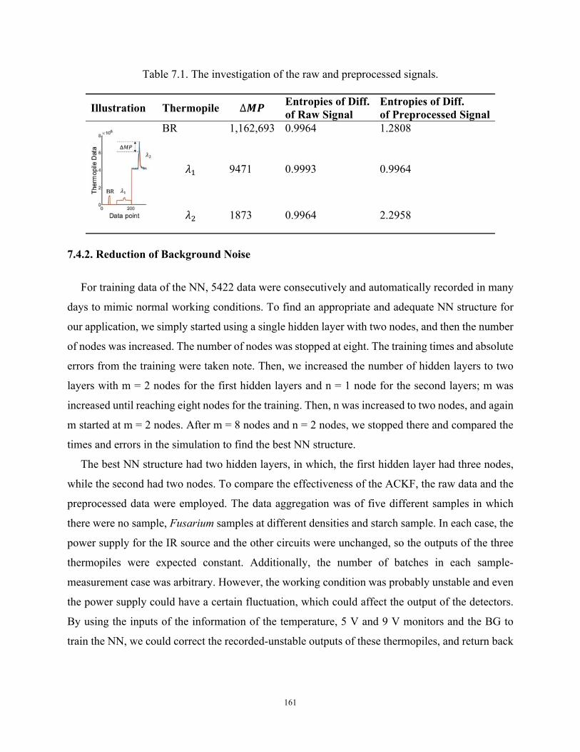
161
Table 7.1. The investigation of the raw and preprocessed signals.
Illustration Thermopile ∆𝑴𝑷 Entropies of Diff. of Raw Signal
Entropies of Diff. of Preprocessed Signal
BR 1,162,693 0.9964 1.2808
𝜆 9471 0.9993 0.9964
𝜆 1873 0.9964 2.2958
7.4.2. Reduction of Background Noise
For training data of the NN, 5422 data were consecutively and automatically recorded in many
days to mimic normal working conditions. To find an appropriate and adequate NN structure for
our application, we simply started using a single hidden layer with two nodes, and then the number
of nodes was increased. The number of nodes was stopped at eight. The training times and absolute
errors from the training were taken note. Then, we increased the number of hidden layers to two
layers with m = 2 nodes for the first hidden layers and n = 1 node for the second layers; m was
increased until reaching eight nodes for the training. Then, n was increased to two nodes, and again
m started at m = 2 nodes. After m = 8 nodes and n = 2 nodes, we stopped there and compared the
times and errors in the simulation to find the best NN structure.
The best NN structure had two hidden layers, in which, the first hidden layer had three nodes,
while the second had two nodes. To compare the effectiveness of the ACKF, the raw data and the
preprocessed data were employed. The data aggregation was of five different samples in which
there were no sample, Fusarium samples at different densities and starch sample. In each case, the
power supply for the IR source and the other circuits were unchanged, so the outputs of the three
thermopiles were expected constant. Additionally, the number of batches in each sample-
measurement case was arbitrary. However, the working condition was probably unstable and even
the power supply could have a certain fluctuation, which could affect the output of the detectors.
By using the inputs of the information of the temperature, 5 V and 9 V monitors and the BG to
train the NN, we could correct the recorded-unstable outputs of these thermopiles, and return back

162
more stable outputs. Firstly, we checked the efficiency of the ACKF by comparing the training
times and the absolute errors of the 𝜆 and 𝜆 thermopiles. The results are depicted in Table 7.2.
Table 7.2. The training results of raw data vs. preprocessed (prep.) data.
𝝀𝟏 𝝀𝟐
Raw data Prep. Data Raw Data Prep. Data
Time 12 min 09 sec 00 min 46 sec 9 min 13 sec 1 min 00 sec
Error 2.7453 × 10⁴ 1.4374 × 10⁴ 2.3999 × 10⁵ 1.76485 × 10⁵
In the training NN, both error and entropy criteria were applied. As mentioned in the entropy
section that the AME may cause the data correction swing even though the AME was optimized
through the weights and biases searching. Figure 7.9 shows the plots of the ACKF preprocessed
data and corrected data of 𝜆 thermopile of using error and entropy as operational criteria.
In the preprocessed MP data of the λ thermopile, Figure 7.8(a) illustrates the results of applying
entropy. Figure 7.9(b) is the close view of Figure 7.9(a) of the four different samples. Similarly,
Figure 7.9(c), (d) show the results when using the AME criterion. The black lines in the plots are
to show the expectation of MP values. The expectation MPs were chosen from view the correlation
of the MP data and the SBGs of the three cooperative thermopiles. The close views show data of
the other four different samples. It can be seen the entropy operating criterion could work better
than the error operating criterion.
Figure 7.9. The ACKF preprocessed (prep.) and corrected max peak (MP) data of 𝜆 thermopile of using entropy and absolute-mean error function (AME) criteria respectively. (a) Full view of the data achieved by entropy criterion; (b) close view of the data batches from
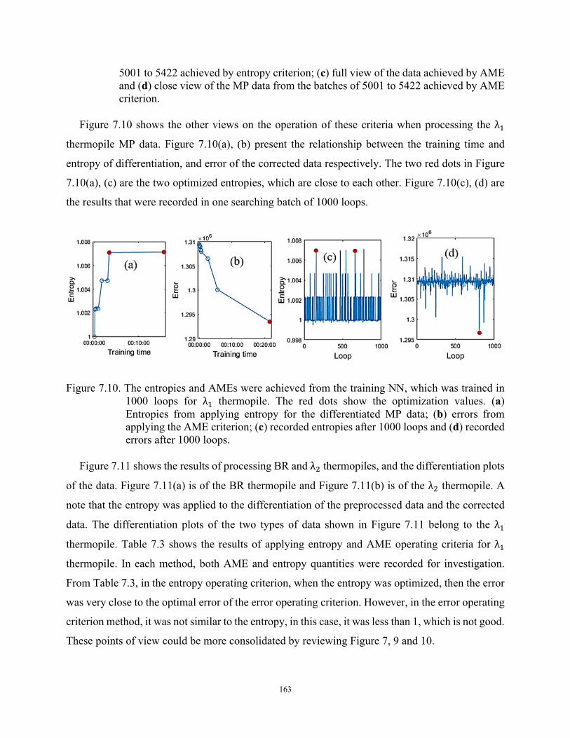
163
5001 to 5422 achieved by entropy criterion; (c) full view of the data achieved by AME and (d) close view of the MP data from the batches of 5001 to 5422 achieved by AME criterion.
Figure 7.10 shows the other views on the operation of these criteria when processing the λ
thermopile MP data. Figure 7.10(a), (b) present the relationship between the training time and
entropy of differentiation, and error of the corrected data respectively. The two red dots in Figure
7.10(a), (c) are the two optimized entropies, which are close to each other. Figure 7.10(c), (d) are
the results that were recorded in one searching batch of 1000 loops.
Figure 7.10. The entropies and AMEs were achieved from the training NN, which was trained in 1000 loops for λ thermopile. The red dots show the optimization values. (a) Entropies from applying entropy for the differentiated MP data; (b) errors from applying the AME criterion; (c) recorded entropies after 1000 loops and (d) recorded errors after 1000 loops.
Figure 7.11 shows the results of processing BR and λ thermopiles, and the differentiation plots
of the data. Figure 7.11(a) is of the BR thermopile and Figure 7.11(b) is of the λ thermopile. A
note that the entropy was applied to the differentiation of the preprocessed data and the corrected
data. The differentiation plots of the two types of data shown in Figure 7.11 belong to the λ
thermopile. Table 7.3 shows the results of applying entropy and AME operating criteria for λ
thermopile. In each method, both AME and entropy quantities were recorded for investigation.
From Table 7.3, in the entropy operating criterion, when the entropy was optimized, then the error
was very close to the optimal error of the error operating criterion. However, in the error operating
criterion method, it was not similar to the entropy, in this case, it was less than 1, which is not good.
These points of view could be more consolidated by reviewing Figure 7, 9 and 10.
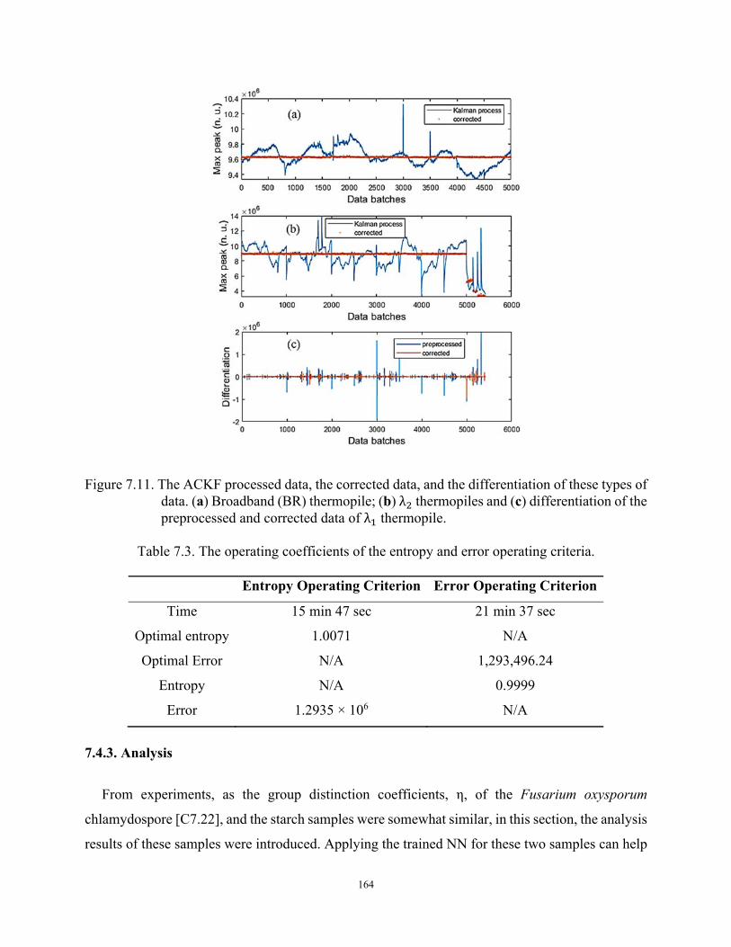
164
Figure 7.11. The ACKF processed data, the corrected data, and the differentiation of these types of data. (a) Broadband (BR) thermopile; (b) λ thermopiles and (c) differentiation of the preprocessed and corrected data of λ thermopile.
Table 7.3. The operating coefficients of the entropy and error operating criteria.
Entropy Operating Criterion Error Operating Criterion
Time 15 min 47 sec 21 min 37 sec
Optimal entropy 1.0071 N/A
Optimal Error N/A 1,293,496.24
Entropy N/A 0.9999
Error 1.2935 × 10⁶ N/A
7.4.3. Analysis
From experiments, as the group distinction coefficients, η, of the Fusarium oxysporum
chlamydospore [C7.22], and the starch samples were somewhat similar, in this section, the analysis
results of these samples were introduced. Applying the trained NN for these two samples can help

165
to correct or calibrate the data of the three thermopiles. Figure 7.12 shows the ACKF preprocessed
data and corrected data of the two samples, which were measured in 50 batches.
From the figure, one can see that the output data of BR were very stable and the correction
process calibrates the data. Applying Equation (7.11), the group distinction coefficients of the two
samples could be found. Figure 7.13(a) shows 𝜂 and 𝜂 plots. It can be seen that
𝜂 and 𝜂 were very close to each other. To determine the number of Fusarium in the
trap, Equation (12) was employed. Figure 7.13(b) depicts the relation of the number of Fusarium
and log(,
) in case of applying data of 𝜆 thermopile.
Figure 7.12. The ACKF preprocessed and corrected data of Fusarium and starch. (a) BR thermopile case; (b) 𝜆 thermopile case and (c) 𝜆 thermopile case.
The fitted curve in Figure 7.13(b) was formed by applying data of the Fusarium samples, which
their known quantities (N):
𝑓 = fitting(log(,
), N) (7.24)
As the group distinction coefficients of Fusarium and starch are close to each other, thus it can
cause confusion at certain times. Table 7.4 shows the means of the group distinction coefficients,
the absolute errors, and the relative errors of Fusarium and starch. From the table, one can see these
values were very close to each other.

166
Figure 7.13. Using data of different Fusarium samples and starch sample measured by 𝜆 thermopile. (a) 𝜂 and 𝜂 and (b) the fitted curve of the known-in-advance Fusarium samples, the interpolation and extrapolation of the unknown-different Fusarium and starch samples. * Fusa. 0 stands for the known-in-advance Fusarium sample. Fusa. 1 and Fusa. 2 are two unknown-quantity samples.
Table 7.4. Group distinction coefficient.
Fusarium Starch
η 1.125 1.31
∆𝜂 0.110 0.06
𝜀 9.8% 4.6%
To improve the fidelity, the broadband thermopile was used. We investigated the other samples
of starch and Fusarium that their quantities were unknown in advance. Making an assumption that
all the samples were Fusarium, we could find the sample quantities Nx by replacing log( ) into
𝑓 of Equation (7.24). Figure 7.13(b) illustrates the extrapolated and interpolated values of the
new samples. From the data of the BR thermopile and the numbers of known-in-advance F. samples
(Fusa. 0), the fitted curve was formed:
𝑓 = fitting(N, log(,
)) (7.25)
Additionally, it is necessary to form the lateral fitted curves for the max and min data points,
which can be seen from the error boxes. error1 and error2 are the errors of the numbers of the

167
Fusarium oxysporum chlamydospore and log10(,
) respectively. Thus, the lateral-fitted curves
are:
𝑓 𝑚𝑎𝑥 = fitting(N + error1, log(,
) + error2) (7.26)
𝑓 𝑚𝑖𝑛 = fitting(N – error1, log(,
) – error2) (7.27)
In Equations (7.26) and (7.27), error1 and error2 are the errors of the quantity number of
Fusarium sample N and log(,
) respectively. The lateral curves will create a validation area
(VA). In the case of investigating new measurement, if the point of the quantity number N and
log(,
) is in the VA and η of the sample is in the range of 1.125 ± 0.110, we could conclude that
the sample is Fusarium. Drawing the points of (Nx, log( ,
,) ) is presented in Figure 7.14. The
figure also provides a visual view of the lateral curve and the VA. In Figure 7.14, the points of
starch samples were out of the VA, so along with η of starch, we could go to a conclusion with
more confident and reliable. For the other two Fusarium samples, we could see that almost all of
the measurement points were in the VA, except few points on the left of the figure.
Figure 7.14. 𝑓 = fitting (N, log(,
)) and the validation area formed by the lateral curves of
Equations (7.26) and (7.27).

168
7.4.4. Discussion
The ACKF helps to reduce thermal noise and burst noise well. To be able to fix the outliers of
BG or peak data, at least some reference data points were not affected by the outliers. From these
reference data points, the ACKF could eliminate the outliers. In reality, there are cases that the
ACKF cannot fix the error data (Figure 7.8(f)), as the outliers happen too close to each other.
Therefore, the reference data points are covered by the burst noise. As a result, the error data cannot
adequately be fixed. Besides, from our experiments, we found that the ACKF could also help to
reduce the time to search the global minima for the NN. This could be explained as the thermal
noise and burst noise occurring in the BG noise were filtered very well by the ACKF (Section 4.1),
so the NN could go to the global minima faster. The evidence of this point of view can be seen in
Table 7.2.
Entropy is not only a useful tool to evaluate the work of Kalman filter, but also can be applied
as an operational criterion to replace the other criteria such as the mean absolute error. The results
in Sections 4.1 and 4.2 show the efficiency of the entropy. From Figure 7.8(c),(d), and Table 7.2,
although the error was the smallest after 1000 loops, the visual results were not what we expected.
The corrected points fluctuated surrounding the expected lines. Entropy was applied to the
differentiation of the preprocessed and corrected MP data rather than being applied directly to these
data. Loosely speaking, the differentiation step helped to remove the difference in the magnitude
of these MP data, as we only focused on the BG noise. The information left was mainly the BG
noise, which influenced the MP data (Figure 7.10(c)). Entropy now reveals how much BG noise is
removed by comparing the entropies of the differentiation of the preprocessed and corrected MP
data.
Figure 7.12 presents the results when the trained NN was used to correct the error data of
Fusarium and starch in which these samples were measured in many batches. In Figure 7.11(a),
one can see that the NN adjusted the MP of both samples. In Figure 7.11(b), (c), the MP data of
starch achieved the largest errors as they lasted from around 0.6 × 10⁶ to 1.7 × 10⁶ in the case of 𝜆
thermopile, and from around 4.3 × 10⁶ to 9.2 × 10⁶ in the case of 𝜆 thermopile.
As the group-distinction coefficient of Fusarium and starch were very similar, the addition of
another thermopile detector, the BR thermopile, could help to distinguish better these two samples.
Figure 7.13 shows that some Fusarium points were out of the VA. This could be explained that in
the data there were outliers, which the ACKF could not correct them. The figure also introduced a

169
case that the starch point was in the VA. However, in general, one could see that most of the
experiment points were in the VA, so the device could distinguish the Fusarium sample from other
samples. With an adding detector, the ability of the device could be expanded. It could help to
detect the group of many more substances.
The group-distinction coefficient of the starch was found in this work was a little bit different
from the value in [C7.20], 0.9390 ± 0.0732. This could be explained that the moistures of the starch
samples used in this work and in [C7.20] were different. A slight change in moisture of the starch
sample might affect its group-distinction coefficient.
7.5. Conclusions
The proposed adaptive-cognitive Kalman filter worked well to reduce the thermal noise and burst
noise. The background noise could be mitigated by applying a neural network. The entropy could
be applied to replace the mean absolute error as an operational condition. The upgraded device
increased the reliability and precision of the current Fusarium detection and quantifying by
applying the proposed techniques. Additionally, by adding one more thermopile, the group
coefficients of substances were more distinct. This assisted the device to distinguish different
substances easier with higher accuracy compared to the use of only two thermopiles.
References
[C7.1] M. Nucci and E. Anaissie, “Fusarium Infections in Immunocompromised Patients,”
Clinical Microbiology Reviews, vol. 20, no. 4, pp. 695–704, Oct. 2007.
[C7.2] J. Evans, D. Levesque, A. de Lahunta, and H. E. Jensen, “Intracranial fusariosis: a novel
cause of fungal meningoencephalitis in a dog,” Vet. Pathol., vol. 41, no. 5, pp. 510–514,
Sep. 2004.
[C7.3] R. D. Martyn, “Fusarium Wilt of Watermelon: 120 Years of Research,” in Horticultural
Reviews: Volume 42, J. Janick, Ed. Hoboken, New Jersey: John Wiley & Sons, Inc., 2014,
pp. 349–442.
[C7.4] E. D. de Toledo-Souza, P. M. da Silveira, A. C. Café-Filho, and M. Lobo Junior,
“Fusarium wilt incidence and common bean yield according to the preceding crop and the
soil tillage system,” Pesq. agropec. bras., vol. 47, no. 8, pp. 1031–1037, Aug. 2012.

170
[C7.5] E. Bauriegel, A. Giebel, and W. B. Herppich, “Rapid Fusarium head blight detection on
winter wheat ears using chlorophyll fluorescence imaging,” Journal of Applied Botany
and Food Quality, vol. 83, no. 3, pp. 196-203, August 2010.
[C7.6] A. Adesemoye et al., “Current knowledge on Fusarium dry rot of citrus,” Citrograph 29,
p. 6, Nov. 2011.
[C7.7] N. A. Foroud, S. Chatterton, L. M. Reid, T. K. Turkington, S. A. Tittlemier, and T.
Gräfenhan, “Fusarium Diseases of Canadian Grain Crops: Impact and Disease
Management Strategies,” in Future Challenges in Crop Protection Against Fungal
Pathogens, A. Goyal and C. Manoharachary, Eds. New York, NY: Springer New York,
pp. 267–316, 2014.
[C7.8] BASF Canada Inc., “Fusarium Management Guide.” BASF Canada Inc. Available:
https://agro.basf.ca. Accessed: 01-Oct.-2019.
[C7.9] C. Marinach-Patrice et al., “Use of mass spectrometry to identify clinical Fusarium
isolates,” Clinical Microbiology and Infection, vol. 15, no. 7, pp. 634–642, Jul. 2009.
[C7.10] A. Salman, L. Tsror, A. Pomerantz, R. Moreh, S. Mordechai, and M. Huleihel, “FTIR
spectroscopy for detection and identification of fungal phytopathogenes,” Spectroscopy,
vol. 24, no. 3–4, pp. 261–267, 2010.
[C7.11] E. Tamburini, E. Mamolini, M. De Bastiani, and M. Marchetti, “Quantitative
Determination of Fusarium proliferatum Concentration in Intact Garlic Cloves Using
Near-Infrared Spectroscopy,” Sensors, vol. 16, no. 7, p. 1099, Jul. 2016.
[C7.12] J. S. West, G. G. M. Canning, S. A. Perryman, and K. King, “Novel Technologies for the
detection of Fusarium head blight disease and airborne inoculum,” Trop. plant pathol.,
vol. 42, no. 3, pp. 203–209, Jun. 2017.
[C7.13] P. Papireddy Vinayaka et al., “An Impedance-Based Mold Sensor with on-Chip Optical
Reference,” Sensors, vol. 16, no. 10, p. 1603, Sep. 2016.
[C7.14] C. G. Dobbs, “ON THE PRIMARY DISPERSAL AND ISOLATION OF FUNGAL
SPORES,” New Phytol, vol. 41, no. 1, pp. 63–69, May 1942.
[C7.15] J. J. Ooka and T. Kommedahl, “Winter and rain dispersal of Fusarium moniliforme in
corn fields,” Phytopathology, vol. 67. pp. 1023–1026, 1977.

171
[C7.16] T. Quesada, J. Hughes, K. Smith, K. Shin, P. James, and J. Smith, “A Low-Cost Spore
Trap Allows Collection and Real-Time PCR Quantification of Airborne Fusarium
circinatum Spores,” Forests, vol. 9, no. 10, p. 586, Sep. 2018.
[C7.17] J. Lacey, “Philip herries gregory (1907–1986),” Grana, vol. 25, no. 3, pp. 159–160, Dec.
1986.
[C7.18] P. H. Gregory, E. J. Guthrie, and M. E. Bunce, “Experiments on Splash Dispersal of
Fungus Spores,” Journal of General Microbiology, vol. 20, no. 2, pp. 328–354, Apr. 1959.
[C7.19] Gary C. Begstrom Melissa D. Keller and Elson J. Sheilds, “The aerobiology of Fusarium
graminearum,” Aerobiologia, vol. 30, pp. 123–136, Nov. 2013.
[C7.20] Son Pham, Anh Dinh, and Khan Wahid, “A Nondispersive Thermopile Device with an
Innovative Method to Detect Fusarium Spores,” IEEE Sensors Journal, vol. 19, issue 19,
pp. 8657-8667, Jun. 2019
[C7.21] J. M. Parnis and K. B. Oldham, “Beyond the Beer-Lambert Law: The Dependence of
Absorbance on Time in Photochemistry,” J. of Photochem. & Photobio., A: Chem., vol.
267, pp. 6-10, 2103. Available: https://doi.org/10.1016/j.jphotochem.2013.06.006.
[C7.22] J. F. Leslie and B. A. Summerell, The fusarium laboratory manual, 1st Edition, Ames,
Iowa: Blackwell Pub, 2006.
[C7.23] Texas Instruments, “Noise Analysis in Operational Amplifier Circuits,” Texas Instrument,
2007. [Online]. Available: http://www.ti.com/. [Accessed: 01-Aug-2019].
[C7.24] G. Vasilescu, “Physical Noise Sources,” in Electronic Noise and Interfering Signals -
Principles and Applications, Printed in Germany: Springer, 2004, pp. 45–67.
[C7.25] M. Á. Raposo-Sánchez, J. Sáez-Landete, and F. Cruz-Roldán, “Analog and digital filters
with α-splines,” Digital Signal Processing, vol. 66, pp. 1–9, Jul. 2017.
[C7.26] L. Luu and A. Dinh, “Using Moving Average Method to Recognize Systole and Diastole
on Seismocardiogram without ECG Signal,” in 2018 40th Annual International
Conference of the IEEE Engineering in Medicine and Biology Society (EMBC), Honolulu,
USA, pp. 3796–3799, June 2018.
[C7.27] E. B. Moullin and H. D. M. Ellis, “The spontaneous background noise in amplifiers due
to thermal agitation and shot effects,” Institution of Electrical Engineers - Proceedings of
the Wireless Section of the Institution, vol. 9, no. 26, pp. 81–106, 1934.

172
[C7.28] L. Dan, W. Xue, W. Guiqin, and Q. Zhihong, “A Methodological Approach for Detecting
Burst Noise in the Time Domain,” International Journal of Electronics and
Communication Engineering, vol. 3, no. 10, p. 5, 2009.
[C7.29] D. Deschrijver, L. Knockaert, and T. Dhaene, “Improving robustness of vector fitting to
outliers in data,” IEEE Electronics Letters, vol. 46, no. 17, pp. 1200–1201, Aug. 2010.
[C7.30] G. M. Siouris, Guanrong Chen, and Jianrong Wang, “Tracking an incoming ballistic
missile using an extended interval Kalman filter,” IEEE Transactions on Aerospace and
Electronic Systems, vol. 33, no. 1, pp. 232–240, Jan. 1997.
[C7.31] Z. Zu-Tao and Z. Jia-Shu, “Sampling strong tracking nonlinear unscented Kalman filter
and its application in eye tracking,” Chinese Phys. B, vol. 19, no. 10, p. 104601, Oct. 2010.
[C7.32] S. Yin, J. H. Na, J. Y. Choi, and S. Oh, “Hierarchical Kalman-particle filter with
adaptation to motion changes for object tracking,” Computer Vision and Image
Understanding, vol. 115, no. 6, pp. 885–900, Jun. 2011.
[C7.33] H. Zhang, G. Dai, J. Sun, and Y. Zhao, “Unscented Kalman filter and its nonlinear
application for tracking a moving target,” Optik, vol. 124, no. 20, pp. 4468–4471, Oct.
2013.
[C7.34] A. Motwani, S. K. Sharma, R. Sutton, and P. Culverhouse, “Interval Kalman Filtering in
Navigation System Design for an Uninhabited Surface Vehicle,” The Journal of
Navigation, vol. 66, no. 5, pp. 639–652, Sep. 2013.
[C7.35] S. Pham and A. Dinh, “Using the Kalman Algorithm to Correct Data Errors of a 24-Bit
Visible Spectrometer,” Sensors, vol. 17, no. 12, p. 2939, Dec. 2017.
[C7.36] D. Lautier, “The Kalman filter in finance: An application to term structure models of
commodity prices and a comparison between the simple and the extended filters,” IDEAS
Working Paper Series from RePEc; St. Louis, 2002.
[C7.37] A. Bensoussan, Estimation and Control of Dynamical Systems, vol. 48. Cham: Springer
International Publishing, 2018.
[C7.38] Amir Amani and Dariush Mohammadyani, Artificial Neural Networks: Applications in
Nanotechnology. INTECH Open Access Publisher, 2011.
[C7.39] K. P. Murphy, Machine learning: a probabilistic perspective. Cambridge, MA: MIT
Press, 2012.
[C7.40] Y. Zhang, Machine Learning. INTECH Open Access Publisher, 2010.

173
[C7.41] C. Nwankpa, W. Ijomah, A. Gachagan, and S. Marshall, “Activation Functions:
Comparison of trends in Practice and Research for Deep Learning,” Cornell University,
p. 20, Nov. 2018.
[C7.42] K. Suzuki, Ed., Artificial Neural Networks - Architectures and Applications. InTech,
2013.
[C7.43] K. Suzuki, Ed., Artificial Neural Networks - Methodological Advances and Biomedical
Applications. InTech, 2011.
[C7.44] S. Amari and A. Cichocki, “Adaptive blind signal processing-neural network
approaches,” Proceedings of the IEEE, vol. 86, no. 10, pp. 2026–2048, Oct. 1998.
[C7.45] A. Zaatri, N. Azzizi, and F. L. Rahmani, “Voice Recognition Technology Using Neural
Networks,” Journal of New Technology and Materials, vol. 277, no. 2414, pp. 1–5, Jun.
2015.
[C7.46] C.-C. Huang, C.-F. J. Kuo, C.-T. Chen, C.-C. Liao, T.-T. Tang, and T.-L. Su, “Inspection
of appearance defects for polarizing films by image processing and neural networks,”
Textile Research Journal, vol. 86, no. 15, pp. 1565–1573, Sep. 2016.
[C7.47] J. A. Villacorta-Atienza and V. A. Makarov, “Neural Network Architecture for Cognitive
Navigation in Dynamic Environments,” IEEE Transactions on Neural Networks and
Learning Systems, vol. 24, no. 12, pp. 2075–2087, Dec. 2013.
[C7.48] Northumbria Optical, “Narrow Band Pass,” Northumbria Optical Coatings Ltd, 2018.
[Online]. Available: https://www.noc-ltd.com. [Accessed: 01-Aug-2019].
[C7.49] “2M Thin Film Based Thermopile Detector,” Dexter Research Center. [Online].
Available: https://www.dexterresearch.com/. [Accessed: 01-Aug-2019].
[C7.50] Micro-Hybrid, “Infrared Radiation Source JSIR350-4-AL-C-D3.7-A5-I,” Micro-Hybrid.
[Online]. Available: http://www.eoc-inc.com/micro-hybrid/IRSource/JSIR350-4-AL-C-
D3.7-A5-l.pdf. [Accessed: 01-Aug-2019].
[C7.51] Analog Devices, “Zero-Drift, Single-Supply, Rail-to-Rail Input/Output Operational
Amplifier AD8628/AD8629/AD8630,” Analog Device, 2014. [Online]. Available:
analog.com. [Accessed: 01-Aug-2019].
[C7.52] Texas Instruments, “OPAx320x Precision, 20-MHz, 0.9-pA, Low-Noise, RRIO, CMOS
Operational Amplifier with Shutdown 1,” Texas Instrument, 2016. [Online]. Available:
http://www.ti.com. [Accessed: 01-Aug-2019].

174
[C7.53] “24-Bit µPower No Latency ∆ΣTM ADC in SO-8,” Analog Device. [Online]. Available:
https://www.analog.com/media/en/technical-documentation/data-sheets/2400fa.pdf.
[Accessed: 01-Jun-2019].
[C7.54] Microchip, “Atmel 8-Bit Microcontroller with 4/8/16/32kbytes In-System Programmable
Flash,” https://www.microchip.com. [Online]. Available: https://www.microchip.com.
[Accessed: 01-Aug-2019].
[C7.55] D. Sh. Sabirov, “Information entropy changes in chemical reactions,” Computational and
Theoretical Chemistry, vol. 1123, pp. 169–179, Jan. 2018.
[C7.56] C. E. Shannon, “A Mathematical Theory of Communication,” SIGMOBILE Mob.
Comput. Commun. Rev., vol. 5, no. 1, pp. 3–55, Jan. 2001.
[C7.57] S. Aydın, H. M. Saraoğlu, and S. Kara, “Log Energy Entropy-Based EEG Classification
with Multilayer Neural Networks in Seizure,” Ann Biomed Eng, vol. 37, no. 12, pp. 2626–
2630, Dec. 2009.

175
8. Conclusion and Future Work
8.1. Summary and Conclusion
First, the thesis work proposes a method to create a 24-bit VIS spectrometer which can serve
for sample analysis. The Beer-Lambert law is used to analyse samples. The problem of unstable
output of the light sensor arises since battery is used to power this portable device. The battery
energy eventually reduces to a level at which the output of the regulators becomes unstable. This
leads to the un-stability of the light intensity which results in the error in the sample spectra
analysis. Using a second light sensor to monitor the light source along with the Kalman algorithm
reduces errors in the data and increases performance of the spectrometer. The proposed method of
applying Kalman algorithm can be applied in any electronic system facing similar problems.
Beer-Lambert law is used again in a non-dispersive thermopile device to detect and analyze
Fusarium spore in the air. The designed device and detection method overcome the drawbacks
from other suggested detection methods in the past. The disadvantages of previous devices are
bulky and expensive (FTIR spectroscopy or mass spectrometer), requirement of well-trained
operators, and long analysis time. A group distinction coefficient was derived from the Beer-
Lambert. Each substance (or sample) should have its own distinct coefficient in the spectrum
analysis. To estimate this coefficient, it is required to have two distinct absorbent wavelengths of
the target samples. These two wavelengths can be determined from the IR spectra of the samples.
For the purpose of Fusarium spore detection, the two chosen wavelengths are 𝜆 =6.088µm and
𝜆 =9.487µm. Based on these wavelengths, two thermopiles which can respectively react with these
wavelengths are used to measure the absorbance level of the Fusarium in the detection device.
Since airborne is a common method of spreading of the fungus, the detection device must sample
the air which is drawn into and passed through a high voltage trap. The trap creates electrostatic
charges on the two silver coated mirrors. The electrostatic charges catch the particles in the air for
detection and analysis. The target Fusarium spores have specific size therefore it is essential to
remove unwanted particles which may cause interference and difficulty in analyzing the data. A
new method of combining a quad-inlet cyclone separator and the high voltage trap to make a
bandpass particle filter is proposed. The features of the filter are simulated and investigated using
the COMSOL Multiphysics software. Appropriate parameters for a filter prototype are determined.

176
The quad-inlet cyclone is printed by a 3D printer and the high voltage trap is made by resin casting
method. The prototype filter is successfully tested in near to practical environment conditions.
In data analysis of the detection device, the challenging is the interference of noises. These
noises include thermal noise, burst noise, and background noises. Among the three, background
noise affects the most to the detection and analysis as its effect results in the error in the thermopile
data. The neural network approach is developed and used to correct the error. To support for the
correction, a temperature sensor and two-voltage monitor modules are installed into the device to
record the operating conditions. The training data for the neural network are collected in one week
in order to record as much as possible the information of real operating conditions. The thermopile
data, the information of the operating conditions, and the background noise extracted from the
thermopile data are used to train the neural network. The trained neural network is used for error
corrections. The results prove the performance of the proposed method in error correction on data
affected by noises.
In the detection, there are cases in which the group distinction coefficients of two or more
samples can be similar to each other such as Fusarium and starch in the experiments. The similarity
of the coefficients may lead to incorrect detection. To overcome this problem, a set of three
thermopiles (broadband (1µm to 20µm), 𝜆 , and 𝜆 thermopiles) is used in the upgraded device
from the previous version of the Fusarium detection device. The addition of the broadband
thermopile assists in distinguishing the samples having similar group-distinction coefficients. In
addition, to increase the precision, an adaptive-cognitive Kalman filter is designed to process
thermal and burst noises. The efficiency of method is proven through the experiment results.
In general, the main contribution of the research is providing the group-distinction coefficient
formula which is the key to build up the Fusarium detection system, a comprehensive approach to
build a portable device to detect and analyze biology objects in the air. The approach includes
selecting wavelengths, building filter and amplifiers, noise processing, and data analysis. Even the
focus of this thesis work is to detect and quantify the Fusarium spores in the air to reduce the
potential loses caused by Fusarium, the methodology can be applied in various areas including
agriculture security, food security, or human-living environment.

177
8.2. Suggestions for Further Studies
Although the introduced method has been proven through building of the prototype and
experimental results, more tests should be conducted in the crop fields to observe the other effects
of the real environment on the device. Currently, the data collected from the device by the Atmel
328P microcontroller must be sent to a computer for further processing. The Atmel 328P could be
replaced by another powerful microprocessor. The microcontroller then can take the role of
collecting, processing data, and making detection decision. Noise process is still very complicated.
Conducting more research on building better amplifiers or selecting other detectors can increase
accuracy and precision of the device. Finding ways to reduce the size of the device can provide
more applications for this detection method. For example, if this device is small enough, it can be
attached to a drone to cover a larger area and greatly reduce the expense.