developing a framework for modeling underwater vehicles in

Developing a Framework for Modeling Underwater Vehicles in Modelica

Shashank Swaminathan1 Srikanth Saripalli1 1Texas A&M University, College Station, TX, USA, [email protected], [email protected]

Abstract When developing Remotely Operated Vehicles (ROVs), models prove extremely useful in determining design parameters and control strategies. This paper’s goal is to develop a modeling framework for underwater ROVs in Modelica, with integration with the Robotic Operating System (ROS), allowing for quicker prototyping and testing of ROV design and control.

Named the Underwater Rigid Body Library (URBL), the modeling framework treats the effect of water on submerged bodies as interactions with a “field” of water to capture the effects of buoyancy and drag. Its usage is demonstrated by applying it to the BlueROV2, a commercially available ROV from Blue Robotics. Using controller signals to the propellers as system inputs, the model was tested with various motor command profiles to achieve different composite motions. Constant motor commands were provided both from within Modelica and from ROS; the simulation results indicated that the model responded appropriately. Keywords: Underwater, ROV, Modelica, ROS, Framework

1 Introduction 1.1 Relevant Background Remotely Operated Vehicles (ROVs) are vital for the exploration and development of areas that are beyond the reach of humans, particularly in the underwater field. When developing any ROV design, it is helpful to construct a model of the design to provide an idea of its performance. There exist many models of underwater vehicle designs like in (Prestero, 2001), but these models focus specifically upon one vehicle design. There are very few initiatives geared towards modeling a variety of underwater bodies and vehicles (McMillian et al, 1995; Tran et al, 2018), but even these are purpose-built software programs. The aim of this paper is to develop a general-purpose modeling framework in Modelica that can be used to model an ROV design using prebuilt components and has flexibility to grow as a library.

The paper will focus on modeling the ROV based off rigid-body principles, as is done in (Tang, 1999; Wang,

W. et al, 2006). This is as opposed to modeling based on CFD principles, like in (Yang et al, 2016; Wang, C., et al, 2014), as it would be intractable for quick prototyping and control testing. Representing hydrodynamic forces, such as viscous drag and added mass, can be done at varying levels of complexity, as seen in (Yuh, 1990), and (da Silva et al, 2007). As this paper’s focus is on developing a modeling framework, it will only address the most basic of hydrodynamics, while also providing a template for further expansion by the user.

1.2 Objectives The goal for the work described in this paper is to develop a basic framework for mathematically modeling underwater vehicles that can: • Aid the prototyping and testing of vehicle design

and controls. • Be readily integrated with common control and

feedback mechanisms, specifically ROS. • Visualize prototype design and test results via three-

dimensional animation. In Section 2, the modeling framework URBL is

discussed in detail. In Section 3, a demonstration of the modeling framework is done via a use case of modeling a physical ROV. Section 4 follows with verification tests of the model developed from the framework, and the ROS interface capability of the model. Section 5 provides the final remarks and closes the paper.

2 Underwater Rigid Body Library. 2.1 Overview The modeling framework is developed as the Underwater Rigid Body Library (URBL) – the library contains the base functional components to any ROV design. The URBL consists of two major sections – components and interfaces for modeling underwater vehicles, and an external interface to ROS. The URBL components are models to describe rigid body interactions with water; the interface is for a basic propeller.

DOI PROCEEDINGS OF THE 1ST AMERICAN MODELICA CONFERENCE 10.3384/ECP18154157 OCTOBER 9-10, 2018, CAMBRIDGE, MASSACHUSETTS, USA

157

2.2 Rigid Body and Field Model As modeling within Modelica is component-based, it is imperative to develop a rigid body component that can interact with the surrounding submerging fluid environment. To accomplish this, the framework represents the environment via a field. The fluid is assumed to be an incompressible Newtonian fluid. The field is considered to have two primary interactions with the rigid body – one via the buoyancy and the other via fluid drag forces exerted by the fluid on the rigid body. This is written into the model as shown below, with 𝜌𝜌𝑏𝑏𝑏𝑏𝑏𝑏𝑏𝑏 being the density of the rigid body, 𝜌𝜌𝑓𝑓𝑓𝑓𝑓𝑓𝑓𝑓𝑏𝑏 the density of the submergent fluid, 𝜈𝜈𝑣𝑣𝑓𝑓𝑣𝑣𝑣𝑣𝑏𝑏𝑣𝑣𝑓𝑓𝑣𝑣𝑏𝑏 being the coefficient of viscosity, and 𝐴𝐴 being the cross-sectional area of the body.

𝑓𝑓𝑏𝑏𝑓𝑓𝑏𝑏𝑏𝑏𝑏𝑏𝑏𝑏𝑣𝑣 ∶= −𝜌𝜌𝑓𝑓𝑓𝑓𝑓𝑓𝑓𝑓𝑏𝑏𝜌𝜌𝑏𝑏𝑏𝑏𝑏𝑏𝑏𝑏

∙ 𝑚𝑚 ∙ �⃗�𝑔 (1)

𝑓𝑓𝑏𝑏𝑑𝑑𝑏𝑏𝑑𝑑 ∶= −𝜈𝜈𝑣𝑣𝑓𝑓𝑣𝑣𝑣𝑣𝑏𝑏𝑣𝑣𝑓𝑓𝑣𝑣𝑏𝑏 ∙ 𝐴𝐴 ∙ �⃗�𝑣

(2)

Here, �⃗�𝑣 represents the velocity of the body, �⃗�𝑔 the gravitational acceleration, and 𝑚𝑚 the mass. To account for drag torques purely due to angular speed �⃗⃗⃗�𝜔, the following equation is added to the drag computation:

𝜏𝜏𝑏𝑏𝑑𝑑𝑏𝑏𝑑𝑑 = −𝑘𝑘𝑏𝑏𝑑𝑑𝑏𝑏𝑑𝑑 ∙ �⃗⃗⃗�𝜔 (3) where 𝑘𝑘𝑏𝑏𝑑𝑑𝑏𝑏𝑑𝑑 represents the coefficient of drag

rotationally (Wadoo, Kachroo, 2016). The field model dictates the values of the forces

affecting bodies within. The field’s force is applied equally across all elements in the field. However, when dealing with a rigid body, where the only interface available is the Frame of Interest (F.O.I), it is not possible to implement the field in such a manner. Instead, the total force the field applies on the body at the center of mass (CM) is translated to the F.O.I, as seen in Figure 1.

Figure 1 – Translation of buoyant and drag forces from center of mass to frame of interest

The rigid body model itself is extended from the standard MultiBody Library (Otter, 2003). The field model is added to the rigid body model, using the inner and outer qualifiers in Modelica, so that any component constructed from this rigid body model will interact with

the fluid surrounding the component, regardless of design. The Modelica-specific implementation is shown in Appendix B.

2.3 Propeller Model The schematic in Figure 2 captures the torque and

thrust generation in the propeller – the electric motor is captured through the EMF, and the propeller frame captures the momentum exchange between the blades and the water.

Figure 2 - Schematic of propeller structure

The propeller’s rotor is powered by a motor, which in turn is powered by some external source of power. From (Triantafyllou, 2004), the thrust can be written as proportional to the square of the rotor’s angular velocity 𝜔𝜔.

𝐹𝐹𝑣𝑣ℎ𝑑𝑑𝑓𝑓𝑣𝑣𝑣𝑣 ∝ 𝜔𝜔2, 𝐾𝐾𝑇𝑇(𝐽𝐽∗) (4) 𝐾𝐾𝑇𝑇(𝐽𝐽∗) is the thrust coefficient, where 𝐽𝐽∗ is the ratio

between rotor speed (intake speed) and fluid speed (outtake speed). Specifically, 𝐾𝐾𝑇𝑇(𝐽𝐽∗) can be approximated (Triantafyllou, 2004) as follows:

𝐾𝐾𝑇𝑇(𝐽𝐽∗) = 𝛽𝛽1 − 𝛽𝛽2𝐽𝐽∗ (5) 𝐽𝐽∗ = 𝑣𝑣

𝜔𝜔 (6)

Here, 𝛽𝛽1 and 𝛽𝛽2 are functions of the intake and outtake speeds of the water.

Taking 𝑣𝑣 and 𝜔𝜔 as the linear and angular velocities of the propeller along its axis, Equation 4 can be rewritten as follows:

𝐹𝐹𝑣𝑣ℎ𝑑𝑑𝑓𝑓𝑣𝑣𝑣𝑣 ∝ 𝜔𝜔2 (𝛽𝛽1 − 𝛽𝛽2𝑣𝑣𝜔𝜔) (7)

Letting 𝑘𝑘𝑑𝑑, 𝑘𝑘𝑚𝑚 be appropriate constants of proportionality, it can be rewritten as

�⃗�𝐹𝑣𝑣ℎ𝑑𝑑𝑓𝑓𝑣𝑣𝑣𝑣 = 𝑘𝑘𝑚𝑚|𝜔𝜔|(𝑘𝑘𝑑𝑑�⃗⃗⃗�𝜔 − �̂�𝜔 ∙ �⃗�𝑣) 𝑏𝑏𝑏𝑏𝑓𝑓𝑑𝑑 (8)

where 𝑏𝑏𝑏𝑏𝑓𝑓𝑑𝑑 is a constant that indicates the direction of the propeller’s mounting.

While the load torque on the propeller due to thrust can also be represented similarly, for the sake of simplicity, it is approximated by a power balance with constant efficiency 𝜂𝜂, as seen in equation 9. An additional −𝑘𝑘𝑓𝑓𝑏𝑏𝑣𝑣𝑣𝑣�⃗⃗⃗�𝜔 term is added to represent loss purely due to rotor rotation.

PROCEEDINGS OF THE 1ST AMERICAN MODELICA CONFERENCE DOI OCTOBER 9-10, 2018, CAMBRIDGE, MASSACHUSETTS, USA 10.3384/ECP18154157

158

𝜏𝜏𝑙𝑙𝑙𝑙𝑙𝑙𝑙𝑙 = − �⃗�𝐹𝑡𝑡ℎ𝑟𝑟𝑟𝑟𝑟𝑟𝑡𝑡 �̂�𝜔 ∙ �⃗�𝑣

|�⃗⃗⃗�𝜔|𝜂𝜂 − 𝑘𝑘𝑙𝑙𝑙𝑙𝑟𝑟𝑟𝑟�⃗⃗⃗�𝜔 (9)

To better handle when 𝜔𝜔 approaches zero, the �⃗�𝐹𝑡𝑡ℎ𝑟𝑟𝑟𝑟𝑟𝑟𝑡𝑡 is expanded to rewrite the load torque as

𝜏𝜏𝑙𝑙𝑙𝑙𝑙𝑙𝑙𝑙 = −𝑘𝑘𝑚𝑚�⃗�𝑣(𝑘𝑘𝑟𝑟�⃗⃗⃗�𝜔 − �̂�𝜔 ∙ �⃗�𝑣) 𝑏𝑏𝑙𝑙𝑑𝑑𝑟𝑟− 𝑘𝑘𝑙𝑙𝑙𝑙𝑟𝑟𝑟𝑟�⃗⃗⃗�𝜔

(10)

The hydrodynamic effects of added mass and wave drag are not considered in this implementation.

The component diagram implementation in Modelica is displayed in Figure 3. The propeller is split into two sections: the mass of the housing, represented by a URBL body, and the actual propeller rotor, represented by a Rotor1D component. The propeller is driven by an EMF; the Mounting1D components is used to propagate the load torques from the propeller to the main ROV body. The thrust is calculated as a WorldForce component and is applied to the mass of the propeller’s housing directly; the load torque from the water is applied to the rotor as a one-dimensional torque, leaving it uncoupled from the actual ROV.

Figure 3 - Implementation of propeller in Modelica

2.4 Integration of External Controllers Apart from providing the foundational components for modeling ROVs, the URBL’s goal is also to provide easy integration with the Robot Operating System (ROS). ROS (Quigley, 2009) based controllers primarily rely on TCP/IP connections for communication. The URBL thus includes integration for socket communication to ROS, achieved via Modelica’s external C function capability.

The integration is done via a block extended from a Multiple-Input-Multiple-Output (MIMO) block from the Modelica Standard Library. The extended block calls upon an external C function based on a time sampler function; the C function returns an array of control values read from the incoming information

queue buffer on the socket port. The socket uses TCP protocol for communication, allowing for explicit ordering of the flow of information – as opposed to UDP protocol. The block contains parameters to set the IP and port of the external controller. To have ROS interact with the model, a ROS node running a TCP socket was also written, allowing the ROS architecture to communicate with the model by using the node-socket connection as a relay point. The flow of data is shown in Figure 4.

Figure 4 - Schematic of Data Flow between Modelica and ROS

2.5 Package Structure Figure 5 shows the package structure of the URBL.

Figure 5 - Package Structure of the URBL


159

2.6 Development Review The construction of the modeling framework was done in Ubuntu 16.04 using Wolfram SystemModeler (SystemModeler, Wolfram). The distribution of ROS used for testing integration capabilities with control platforms was ROS Kinetic. As the mechanism for connecting ROS to Modelica was based on using TCP sockets, and the build of the model was done in a Linux environment, the ROS connectivity is currently only usable in *nix environments.

3 Application of URBL The URBL’s applicability is tested by modeling a commercially available ROV design – the BlueROV2 (BlueROV2, Blue Robotics), shown in Figure 6.

Figure 6 - Physical BlueROV2

The BlueROV2 has 6 propellers mounted – 2 dual vertical thrusters, and 4 vector-configured thrusters, allowing for 6 DOF. It is controlled via a Pixhawk Autopilot flight controller running ArduSub. The full hardware breakdown of the ROV is shown in Figure 7.

3.1 Frame Modeling The process of assembling the frame of the BlueROV2 physically from kit is replicated when developing the model of its frame. The ROV is built from a base plate, two side plates, and four top plates, each a rigid body of certain uniform density and mass, with points on the body to connect with other parts of the frame. Likewise, the frame model was constructed from several sub-components, each representing one type of frame plate – bottom, side, and top – constructed from URBL rigid bodies, with frames to represent attachment points to other bodies. The resultant total frame is shown in Figure 8.

Figure 8 - Visualization of the ROV model

Figure 7 - Hardware schematic of power and information flow


160

3.2 Propeller Modeling The propeller component for the BlueROV2 is extended from the URBL’s base propeller model. The T200 propellers, used on the BlueROV2, are controlled via Pulse Position Modulation – to approximate this voltage control, a standard signal voltage component was used. Each propeller thus has its own internal electric circuit, with the signal voltage value controlled externally. By doing so, it allows for simpler testing against flight data from the physical ROV – the Pixhawk flight controller on the BlueROV2 sends pulses to the propeller’s driver ESC, which then controls the voltage to the propeller. Hence, the model can now run the same commands sent by the Pixhawk and ESC driver to the propeller.

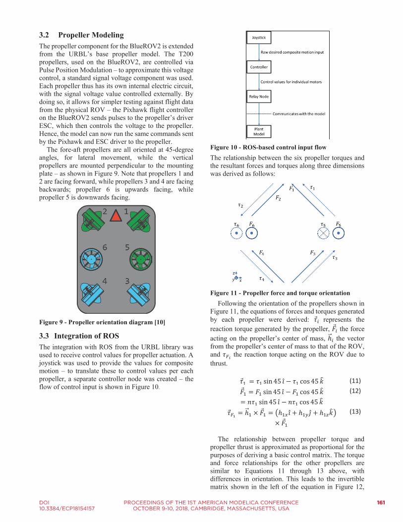
The fore-aft propellers are all oriented at 45-degree angles, for lateral movement, while the vertical propellers are mounted perpendicular to the mounting plate – as shown in Figure 9. Note that propellers 1 and 2 are facing forward, while propellers 3 and 4 are facing backwards; propeller 6 is upwards facing, while propeller 5 is downwards facing.

Figure 9 - Propeller orientation diagram [10]

3.3 Integration of ROS The integration with ROS from the URBL library was used to receive control values for propeller actuation. A joystick was used to provide the values for composite motion – to translate these to control values per each propeller, a separate controller node was created – the flow of control input is shown in Figure 10.

Figure 10 - ROS-based control input flow The relationship between the six propeller torques and the resultant forces and torques along three dimensions was derived as follows:

Figure 11 - Propeller force and torque orientation

Following the orientation of the propellers shown in Figure 11, the equations of forces and torques generated by each propeller were derived: 𝜏𝜏𝑖𝑖 represents the reaction torque generated by the propeller, �⃗�𝐹𝑖𝑖 the force acting on the propeller’s center of mass, ℎ⃗⃗𝑖𝑖 the vector from the propeller’s center of mass to that of the ROV, and 𝜏𝜏𝐹𝐹𝑖𝑖 the reaction torque acting on the ROV due to thrust.

𝜏𝜏1 = 𝜏𝜏1 sin 45 𝑖𝑖̂ − 𝜏𝜏1 cos 45 �̂�𝑘 (11) �⃗�𝐹1 = 𝐹𝐹1 sin 45 𝑖𝑖̂ − 𝐹𝐹1 cos 45 �̂�𝑘

= 𝑛𝑛𝜏𝜏1 sin 45 𝑖𝑖̂ − 𝑛𝑛𝜏𝜏1 cos 45 �̂�𝑘 (12)

𝜏𝜏𝐹𝐹1 = ℎ⃗⃗1 × �⃗�𝐹1 = (ℎ1𝑥𝑥𝑖𝑖̂ + ℎ1𝑦𝑦𝑗𝑗̂ + ℎ1𝑧𝑧�̂�𝑘)× �⃗�𝐹1

(13)

The relationship between propeller torque and

propeller thrust is approximated as proportional for the purposes of deriving a basic control matrix. The torque and force relationships for the other propellers are similar to Equations 11 through 13 above, with differences in orientation. This leads to the invertible matrix shown in the left of the equation in Figure 12,


161

describing the relationship between propeller torques and composite motion. By applying the inverse of this matrix to scale the joystick input, the control values were derived.

3.4 Full ROV Model The full ROV model is created by adding the propeller to the frame model, to provide the methods of propulsion and control to the ROV structure. Selected parameterization of the model is listed in the Appendix A. The completed ROV model is shown in Figure 13.

Figure 13 - Component view of full ROV model in Modelica

4 Testing the ROV Model 4.1 Component Testing The purpose of the component tests is to verify that the component’s individual performance conforms to expectations.

4.1.1 Frame Model Tests When testing the frame, the frame sub-components are placed alone in a body of water, and their size, structure, and motion in response to buoyancy is verified – as each sub-component of the frame is constructed from HDPE (density of 0.97 g/cm3) and symmetric, it has a net buoyancy of 0.2 kg, and therefore is expected to slightly float upwards. The test results do indicate that all sub-components, along with the entire frame, exhibit normal, stable motion in the water field.

4.1.2 Propeller Model Tests This test checks the propeller’s ability to provide thrust to a rigid body in water. To check the model’s stability during rotation, the propeller is made to provide thrust along different axes of rotation to the end of a neutrally buoyant rod. The test results indicate that the propeller proceeds stably and smoothly in all orientations, matching the expected motion.

4.2 Full Model Testing The full ROV model is tested by providing a constant joystick command and evaluating the resulting composite motion of the ROV. The tested composite motion is the forward motion along the X axis – the control values necessary are derived from inverting the matrix in Equation 14.

Figure 14 - Results from testing the full ROV model

In Figure 14, the motion along the X axis is stable, while the motion along the other axes after accounting for drift, linear and angular, is near zero. The drift seen in the rotational values can be attributed to approximations made when constructing the control matrix. The movement seen along the Y axis is due to the net buoyancy of the ROV, and therefore acceptable.

Figure 12 - Relationship between motor torques and composite motion


162

4.3 Testing ROS Integration To test the validity of the model’s external control capability – its connection to ROS – a network of ROS nodes meant to handle both the model’s feedback and the provision of control values is setup. A joystick is used to dictate simple motor control values to the model, via ROS, and the model’s reaction to the values is observed. The joystick sends simple motion commands in the orthogonal directions – lateral motion in the XZ plane – the raw joystick input is seen in Figure 15. The model’s response is displayed in Figure 16. Note that the Figure 15 was recorded from ROS and uses the operating system time; this is different from the simulation time seen in Figure 16.

Figure 15 - Raw Joystick Input

Figure 16 - Results from testing the ROV model when providing motor commands from ROS

The motion along the X axis, and the motion along the Z axis are the values being controlled by the controller. Drift in the rotation angles around the axes is seen, attributable to approximations done in the control matrix. A steady, slow rise is seen along the Y axis (in orange) due to the net buoyancy of the model. The ROV is controlled to move along the XZ plane in accordance with the joystick input. The response of the ROV is as desired, with appropriate motion when moving along each axis separately, as well as when moving in a composite manner in the XZ plane.

5 Conclusions 5.1 Results Summary • The URBL was stably constructed to provide basic

ROV modeling components, as well as ready-to-use integration with ROS

• The URBL was successfully used to model an existing commercially available ROV design, the BlueROV2.

5.2 Further Work

5.2.1 Library Improvements The model of damping was simplified to take the cross-sectional area of a given component in the plane perpendicular to motion as a parameter – an improvement would be to have this area as a changing quantity.

The library’s hydrodynamic models are overall extremely simplified, and so are currently implemented via functions, to increase replaceability. However, this possible interchangeability of hydrodynamic force functions is still limited in scope by the function interface; it could be widened to accept and return any number and kind of inputs and outputs.

For integration with external control mechanisms, the current socket-based integration relies on using Modelica’s external C function capability and poses restrictions on the operating system used for simulation – *nix based distributions, and not Windows. Socket based communication also has limitations in speed – the larger and more computationally intensive the model, the slower the socket-based communication will be. Further improvement can be done by porting this integration to rely on FMI/FMU functionality, instead of C functions and sockets. As noted by a reviewer, there exists another library for providing TCP/IP connections from Modelica via external C-functions, named the Modelica_DeviceDrivers library (Thiele, 2017). The ROS integration in this paper was developed separately from Modelica_DeviceDrivers, though both rely on TCP/IP communications.

5.2.2 Model Improvements When prototyping the design of the model, it is useful to individually model the bodies involved in the ROV structure. However, this adds complexity to the model, and makes it simulate slower. Per a reviewer’s suggestion, to speed up simulation post prototyping, the model should be redrawn with all the rigid bodies consolidated into one central mass, to improve simulation usefulness.

5.2.3 Validation Improvements The motion profiles tested in the standalone model tests could be increased in complexity, from simple movements across and around axes, to more composite motion in three dimensions. The simulation results should also be compared against experimental data from the physical vehicle.

Appendix A – Physical Parameters


163

This is the list of the derived parameters for the electronics enclosure and the battery enclosure.

Appendix B – Modelica Implementation of Field The code for implementing the field is as follows:

Modelica.Mechanics.MultiBody.Forces.WorldForceAndTorque field(animation = false); protected // Fields outer UnderwaterRigidBodyLibrary.Fields.WaterField waterField; outer Modelica.Mechanics.MultiBody.World world; equation // equations of motion r_0 = frame_a.r_0; v_0 = der(r_0); a_0 = der(v_0); w_a = Modelica.Mechanics.MultiBody.Frames.angularVelocity2(frame_a.R); // forces and torques due to fields b_f = waterField.waterBuoyantForce(d = density, m = body.m); f_d = waterField.waterDragForce(v = body.v_0 - Frames.resolve1(frame_a.R, cross(r_CM, w_a)), mu = mu_d, A = A); t_d = Frames.resolve1(frame_a.R, waterField.waterDragTorque(w = w_a, k = k_d)); // applying force and torques due to fields field.force = b_f + f_d; field.torque = cross(Frames.resolve1(frame_a.R, r_CM), b_f) + t_d + cross(Frames.resolve1(frame_a.R, r_CM), f_d); connect(field.frame_b, body.frame_a); connect(frame_a, body.frame_a);

References J. Evans, M. Nahon, Dynamics modeling and performance

evaluation of an autonomous underwater vehicle, Ocean Engineering, Volume 31, Issues 14–15, 2004, Pages 1835-1858, ISSN 0029-8018, doi:10.1016/j.oceaneng.2004.02.006

McMillian, S., Orin, D. E., & McGhee, R. B. (1995). DynaMechs: An object oriented software package for efficient dynamic simulation of underwater robotic vehicles.

Otter, M., Elmquist H, Mattson S. E., “The New Modelica Multibody Library”, Proceedings of the 3rd International Modelica Conference, Linkopig, 2003

Prestero, T. (2001). Development of a six-degree of freedom simulation model for the REMUS autonomous underwater vehicle. In OCEANS, 2001. MTS/IEEE Conference and Exhibition (Vol. 1, pp. 450-455). IEEE.

Quigley, M., Conley, K., Gerkey, B., Faust, J., Foote, T., Leibs, J., ... & Ng, A. Y. (2009, May). ROS: an open-source Robot Operating System. In ICRA workshop on open source software (Vol. 3, No. 3.2, p. 5).

da Silva, J. E., Terra, B., Martins, R., & de Sousa, J. B. (2007, August). Modeling and simulation of the lauv autonomous underwater vehicle. In 13th IEEE IFAC International Conference on Methods and Models in Automation and Robotics. Szczecin, Poland Szczecin, Poland.

Tang, S. C. (1999). Modeling and simulation of the autonomous underwater vehicle, Autolycus (Doctoral dissertation, Massachusetts Institute of Technology).

Thiele, B., Beutlich, T., Waurich, V., Sjölund, M., & Bellmann, T. (2017, July). Towards a Standard-Conform, Platform-Generic and Feature-Rich Modelica Device Drivers Library. In Proceedings of the 12th International Modelica Conference, Prague, Czech Republic, May 15-17, 2017 (No. 132, pp. 713-723). Linköping University Electronic Press.

Tran M., Binns J., Chai S., Forrest A., Nguyen H. (2018) AUVSIPRO – A Simulation Program for Performance Prediction of Autonomous Underwater Vehicle with Different Propulsion System Configurations. In: Mazal J. (eds) Modelling and Simulation for Autonomous Systems. MESAS 2017. Lecture Notes in Computer Science, vol 10756. Springer, Cham

M. Triantafyllou. 2.154 Maneuvering and Control of Surface and Underwater Vehicles (13.49). Fall 2004. Massachusetts Institute of Technology: MIT OpenCourseWare, https://ocw.mit.edu. License: Creative Commons BY-NC-SA

Wadoo, S., & Kachroo, P. (2016). Autonomous underwater vehicles: modeling, control design and simulation. CRC Press.

Wang, C., Zhang, F., & Schaefer, D. (2015). Dynamic modeling of an autonomous underwater vehicle. Journal of Marine Science and Technology, 20(2), 199-212.

Wang, W., & Clark, C. M. (2006). Modeling and simulation of the VideoRay Pro III underwater vehicle. Computer Science and Software Engineering, 66.

Yang, R., Probst, I., Mansours, A., Li, M., & Clement, B. (2016). Underwater vehicle modeling and control application to ciscrea robot. In Quantitative Monitoring of the Underwater Environment (pp. 89-106). Springer, Cham.

Yuh, J. (1990). Modeling and control of underwater robotic vehicles. IEEE Transactions on Systems, man, and Cybernetics, 20(6), 1475-1483.

SystemModeler (2015) Copyright © 2015 Wolfram Research, Inc. http://wolfram.com/system-modeler/

BlueROV2, Blue Robotics, Inc. http://docs.bluerobotics.com/brov2/


164

developing a framework for modeling underwater vehicles in

Documents