developing and evaluating rapid test methods for measuring ... · measuring the sulphate...
TRANSCRIPT

Developing and Evaluating Rapid Test Methods for
Measuring the Sulphate Penetration Resistance of
Concrete in Relation to Chloride Penetration Resistance
by
Ester Karkar
A thesis submitted in conformity with the requirements for the degree of Master of Applied Science
Department of Civil Engineering University of Toronto
© Copyright by Ester Karkar 2011

ii
Developing and Evaluating Rapid Test Methods for Measuring the
Sulphate Penetration Resistance of Concrete in Relation to
Chloride Penetration Resistance
Ester Karkar
Master of Applied Science
Department of Civil Engineering University of Toronto
2011
Abstract
External sulphate attack on concrete can lead to cracking, expansion and sometimes loss of
cohesiveness of hardened cement paste. Therefore, aside from using sulphate resistant
cementitious binders, it is important to design concrete which can resist sulphate penetration. In
this research, both ASTM C1202 and NT Build 492 electrical migration tests were modified such
that sulphate rather than chloride penetration resistances were measured. Modifications included
exposing concrete specimens to Na2SO4 rather than NaCl solutions and measuring the depth of
sulphate penetration visually using BaCl2+KMnO4 rather than AgNO3 solution. Nine concrete
mixtures of varying w/cm, slag replacement and cement types were tested in both original
standard tests and modified tests to evaluate the influence of these material variables on test
results and compare chloride to sulphate results. It was found that while migration coefficients
and total charge passing were lower for sulphate, the influence of material variables were
relatively similar.

iii
Acknowledgments I would like to thank my supervisor Professor Doug Hooton for encouraging and giving me the
great opportunity and privilege of initiating this project, as well as for his guidance and
unconditional support throughout the project. Thanks are also due to Professor Karl Peterson and
Dr. Terry Ramlochan for their assistance in this project. It was an honour to work in the Concrete
Materials Group at the University of Toronto, with such wonderful and supportive group of
individuals. Special thanks are extended to Olga Perebatova and Olga Arevalo-Quintero for their
invaluable help in the laboratory.
For their advice, motivation and delicious coffee breaks, special thanks are extended to my
friends Tarana, Olta, Monica, Gleb, Soley, Mila and Majella.
I would especially like to thank my parents, Suzanne and David, my sister, Claudia and my aunt
Nisreen whose patient love and unconditional support enabled me to accomplish this goal.
Finally, I would like to thank God for giving me the patience and determination to complete this
goal.

iv
Table of Contents
Acknowledgments iii
Table of Contents iv
List of Tables viii
List of Figures xi
Chapter 1 Introduction 1
1 1
1.1 Motivation for Work ........................................................................................................... 1
1.2 Scope and Objectives .......................................................................................................... 1
Chapter 2 Literature Review ........................................................................................................... 2
2 2
2.1 What is External Sulphate Attack? ..................................................................................... 2
2.1.1 Chemical Reactions Involved In External Sulphate Attack .................................... 2
2.1.2 Effects of Sulphate Attack on Concrete .................................................................. 4
2.2 Transport Mechanisms of Aggressive Ions ......................................................................... 4
2.3 Diffusion: Mechanism and Testing ..................................................................................... 5
2.4 Significance of Diffusion Coefficient ................................................................................. 6
2.5 Use of Electrical Test Methods for the Rapid Evaluation of Concrete’s Resistance to the Penetration of Aggressive Ions ..................................................................................... 7
2.5.1 Electrical Migration Tests ....................................................................................... 7
2.5.2 Current Electrical Migration Tests ........................................................................ 13
2.6 Determining Diffusion Coefficient from Resistivity Measurements ................................ 15
2.7 Ionic Movements Occurring During Electrical Migration Tests ...................................... 16
2.7.1 Chloride Migration Tests ...................................................................................... 16

v
2.7.2 Sulphate Migration Tests ...................................................................................... 18
2.8 Drawbacks of Non-Steady-State Electrical Migration Tests ............................................ 19
2.9 Conductance and Resistance ............................................................................................. 21
2.10 Variables Affecting Test Results ...................................................................................... 24
2.10.1 Electrical Conductivities of NaCl and Na2SO4 Electrolytes and Cl- and SO42-
Ions 24
2.10.2 Effects of Degree of Hydration and Water to Cement/Binder Ratio .................... 26
2.10.3 Effects of Supplementary Cementing Materials ................................................... 27
2.10.4 Effect of Cement Type .......................................................................................... 28
2.10.5 Effect of Chemical Binding .................................................................................. 29
Chapter 3 Experimental Procedure ............................................................................................... 31
3 31
3.1 Materials 31
3.1.1 Cementitious Material ........................................................................................... 31
3.1.2 Blast-Furnace Slag ................................................................................................ 31
3.1.3 Fine Aggregate ...................................................................................................... 33
3.1.4 Coarse Aggregate .................................................................................................. 33
3.1.5 Chemical Admixtures ........................................................................................... 33
3.1.6 Water 34
3.2 Mix Designs 34
3.2.1 Mix Proportions .................................................................................................... 34
3.2.2 Casting 35
3.2.3 Curing 36
3.3 Test Procedures 36
3.3.1 Modification of ASTM C1202 .............................................................................. 38
3.3.2 Modification of NT Build 492 .............................................................................. 40

vi
3.3.3 Modified NT Build 492 Test Duration: Test Set-up Enabling the Recording of the Current throughout the Test ............................................................................ 48
3.3.4 Bulk Electrical Resistivity Tests ........................................................................... 52
3.3.5 Compressive Strength Test ................................................................................... 55
Chapter 4 Results: Observations and Discussion .......................................................................... 56
4 56
4.1 Overview 56
4.2 Plastic Properties and Compressive Strengths .................................................................. 58
4.3 Rapid Permeability Test Results ....................................................................................... 60
4.3.1 Total 6 hours Charge, Q6hrs ................................................................................... 60
4.3.2 Qualitatively Evaluating Sulphate Ion Penetrability into Concrete ...................... 65
4.3.3 Resistivity ............................................................................................................. 67
4.4 Rapid Migration Tests- NT Build 492 .............................................................................. 73
4.4.1 Penetration Depths ................................................................................................ 73
4.4.2 Resistivity ............................................................................................................. 89
4.4.3 Modified Test Length ........................................................................................... 92
4.5 Resistivity 98
4.5.1 Initial resistivity .................................................................................................... 98
4.5.2 Relationships between Merlin Resistivity, NT Build 492 and ASTM C 1202 .. 101
Chapter 5 Conclusions and Recommendations ........................................................................... 108
5 108
5.1 Conclusions 108
5.1.1 Effect of Electrolytes on Conductivity ............................................................... 108
5.1.2 Conductivity and Diffusivity: Sulphate vs. Chloride ......................................... 109
5.1.3 Effect of age and water to binder ratio ................................................................ 109
5.1.4 Effect of slag and fly ash replacement ................................................................ 110

vii
5.1.5 Effect of using GU vs. MS and HS cement types ............................................... 111
5.1.6 Identifying Sulphate Penetrations Fronts ............................................................ 112
5.1.7 Relationships between Merlin resistivity, NT Build 492 and ASTM C 1202 .... 112
5.2 Recommendations ........................................................................................................... 113
Chapter 6 References 114
Appendices 119
Appendix A Fine and coarse Aggregate Properties .................................................. 119
Appendix B Mix Designs .......................................................................................... 126
Appendix C ASTM C 1202 Data .............................................................................. 138
Appendix D NT Build 492 Data ............................................................................... 158
Appendix E Merlin and Monfore Electrical Resistivity Data................................... 177
Appendix F Sulphate Profile Grinding and ICP Data .............................................. 182
Appendix G NT Build 492 Modified Test Duration Data ........................................ 186
Appendix H Compressive Strengths ......................................................................... 195

viii
List of Tables Table 2.1 Chloride ion penetrability based on total 6 hrs charge (adapted from ASTM C 1202-
09) ................................................................................................................................................. 14
Table 2.2 Electrical conductivity values of NaCl and Na2SO4 solutions at 2, 5 and 10%
concentrations at 20°C obtained from the “CRC Handbook of Chemistry and Physics”, Haynes
& Lide, 2011. ................................................................................................................................ 25
Table 2.3 Conductivities and diffusion coefficients at infinite dilution of chloride, sulphate and
additional common ionic species present in the pore solution obtained from the “CRC Handbook
of Chemistry and Physics”, Haynes & Lide, 2011. ...................................................................... 26
Table 3.1 Chemical and mineralogical compositions ................................................................... 32
Table 3.2 Physical properties of the fine and coarse aggregates .................................................. 33
Table 3.3 Mix proportions per 1 m3 .............................................................................................. 35
Table 3.4 The influence of the 100 ohm resistor on the actual applied voltage of the ~6.5 months
old, 0.5 w/cm 100% GU cement, concrete specimens tested in NT Build 492 for modified test
durations ........................................................................................................................................ 51
Table 3.5 The influence of the 100 ohm resistor on the applied voltage of the ~6.5 months old,
0.5 w/cm, GU cement with 35 % slag replacement, concrete specimens tested in NT Build 492
for modified test durations ............................................................................................................ 52
Table 4.1 Summary of concrete mixtures tested and their properties ........................................... 57
Table 4.2 Compressive strength and plastic properties of fresh concrete ..................................... 59
Table 4.3 Rapid chloride permeability test specimens, 6 hours charge values, 𝑸𝟔𝒉𝒓𝒔,𝑵𝒂𝒄𝒍
(coulombs). ................................................................................................................................... 60
Table 4.4 Rapid sulphate permeability test specimens, 6 hours charge values 𝑸𝟔𝒉𝒓𝒔,𝑵𝒂𝟐𝑺𝑶𝟒,
(coulombs). ................................................................................................................................... 61

ix
Table 4.5 Percent difference between charge passing through the chloride exposed specimens
and the sulphate exposed specimens ............................................................................................. 62
Table 4.6 Differences in total charge passed during the rapid chloride permeability tests for
selected mixtures ........................................................................................................................... 63
Table 4.7 Differences in total charge passed during the rapid sulphate permeability tests for
selected mixtures ........................................................................................................................... 65
Table 4.8 Modified ASTM C 1202 table suited for sulphate ion penetrability (Adapted from
ASTM C 1202) ............................................................................................................................. 66
Table 4.9 Resistivities obtained from the rapid chloride permeability test specimens, ohm∙m. .. 67
Table 4.10 Resistivities obtained from the rapid sulphate permeability test specimens, ohm∙m. 68
Table 4.11 Differences between the instantaneous resistivities at =5min for selected mixtures.
Rapid chloride permeability test specimens. ................................................................................ 71
Table 4.12 Differences between the instantaneous resistivities at =5min for selected mixtures.
Rapid sulphate permeability test specimens. ................................................................................ 72
Table 4.13 Percent difference between the instantaneous resistivity values of the sulphate and
chloride exposed specimens, measured at t = 5 minutes. ............................................................. 73
Table 4.14 Measured penetration depths of specimens exposed to chlorides at 35 days ............. 74
Table 4.15 Measured penetration depths of specimen exposed to sodium chloride at 56 days ... 74
Table 4.16 Measured penetration depths of specimen exposed to sulphates at 35 days............... 75
Table 4.17 Measured penetration depths of specimen exposed to sulphates at 56 days............... 75
Table 4.18 Average chloride to sulphate penetration depths ratios .............................................. 76
Table 4.19 Summary of chloride migration coefficients, NT Build 492 ...................................... 86
Table 4.20 Differences between chloride migration coefficients for selected mixtures ............... 87

x
Table 4.21 Summary of sulphate migration coefficients, modified NT Build 492 specimens. .... 88
Table 4.22 Differences between sulphate migration coefficients for selected mixtures .............. 89
Table 4.23 Percent difference between the instantaneous resistivity values of the sulphate and
chloride exposed specimens. ......................................................................................................... 92
Table 4.24 Total charge passed through 6.5 month old specimen tested in NT Build 492 with
modified test durations. ................................................................................................................. 94
Table 4.25 Penetration depth of 6.5 month old specimens tested in original and modified NT 492
for longer test durations. ............................................................................................................... 95
Table 4.26 Migration coefficients of the 6.5 months old specimens tested in the original and
modified NT Build 492 for longer test durations of 1, 4 and 9 days. .......................................... 96

xi
List of Figures Figure 2.1 Chloride migration tests: ionic movements due to diffusion. Adapted from Andrade
(1993). ........................................................................................................................................... 17
Figure 2.2 Chloride migration tests: ionic movements due to migration. Adapted from Andrade
(1993). ........................................................................................................................................... 17
Figure 2.3 Chloride migration tests: ionic movements due migration and diffusion. Adapted from
Andrade (1993). ............................................................................................................................ 17
Figure 2.4 Sulphate migration tests: ionic movements under diffusion. Adapted from Andrade
(1993). ........................................................................................................................................... 18
Figure 2.5 Sulphate migration tests: ionic movements under migration. Adapted from Andrade
(1993). ........................................................................................................................................... 19
Figure 2.6 Sulphate migration tests: ionic movements under migration and diffusion. Adapted
from Andrade (1993). ................................................................................................................... 19
Figure 3.1 Schematic of the test plan at each migration test date ................................................ 37
Figure 3.2 Circuit diagram of the NT Build 492 test set-up used in this study ............................ 41
Figure 3.3 Change in total S, Na, K and Ca contents of concrete with change in distance from
sulphate exposed face. Sample was ~6.5 months old, tested in modified NT Build 492 for 4 days
in 10% Na2SO4 solution. Sample properties: 0.5 w/cm, GU cement, 35 % slag, average visible
sulphate front was 3.25 mm deep. ................................................................................................ 46
Figure 3.4 Change in total S, Na, K and Ca contents of concrete with change in distance from
sulphate exposed face. Sample was 56 days old, tested in modified NT Build 492 for 1 day in
10% Na2SO4 solution. Sample properties: 0.4 w/cm, HS cement, average visible sulphate front
was 1.35 mm deep. ........................................................................................................................ 47

xii
Figure 3.5 Circuit diagram of the NT Build 492 with modified test duration set-up used in this
study to record the change in current throughout the modified test duration. Note that all the
blocks connected to the ICP DAS devices are terminal names specific to each device. .............. 49
Figure 3.6 Schematic diagram of the DC (Monfore) bulk electrical resistivity test set-up used in
this study (El-Dieb et al., Unpublished) ........................................................................................ 54
Figure 3.7 Schematic diagram of the measurement method used in the Merlin instrument
(Germann Instruments, 2010) ....................................................................................................... 55
Figure 3.8 Merlin bulk electrical resistivity apparatus
(http://www.germann.org/?strArticle=news) ................................................................................ 55
Figure 4.1 Total charge passing during the rapid sulphate permeability tests vs. total charge
passing during the rapid chloride permeability test ...................................................................... 66
Figure 4.2 Average instantaneous resistivity of the rapid chloride permeability test specimens at
t=5min vs. age, ohm∙m. ................................................................................................................. 69
Figure 4.3 Average instantaneous resistivity of the rapid sulphate permeability test specimens at
t=5min vs. age, ohm∙m. ................................................................................................................. 69
Figure 4.4 Comparison of SO42- and Cl- penetration depths at 35 and 56 days while accounting
for test voltage. .............................................................................................................................. 77
Figure 4.5 Sulphate penetration front of a 56 days old concrete specimen of 0.45 w/cm and
100% HS cement, tested in NT Build 492 testing conditions for 24 hours. ................................. 79
Figure 4.6 Chloride penetration front of a 56 days old concrete specimen of 0.45 w/cm and
100% HS cement, tested in NT Build 492 for 24 hours. .............................................................. 79
Figure 4.7 Sulphate penetration front of a 35 days old concrete specimen of 0.5 w/cm and 100%
MS cement, tested in NT Build 492 testing conditions for 24 hours. ........................................... 80
Figure 4.8 Chloride penetration front of a 35 days old concrete specimen of 0.5 w/cm and 100%
MS cement, tested in NT Build 492 for 24 hours. ........................................................................ 80

xiii
Figure 4.9 Sulphate penetration front of a 35 days old concrete specimen of 0.4 w/cm, MS
cement and 50% slag replacement, tested in NT Build 492 testing conditions for 24 hours. ...... 81
Figure 4.10 Chloride penetration front of a 35 days old concrete specimen of 0.4 w/cm, MS
cement and 50% slag replacement, tested in NT Build 492 for 24 hours. .................................... 81
Figure 4.11 Sulphate penetration front of a 6.5 months old concrete specimen of 0.5 w/cm, GU
cement and 35 % slag replacement, tested in NT Build 492 testing conditions for 24 hours. ..... 82
Figure 4.12 Sulphate penetration front of a 6.5 months old concrete specimen of 0.5 w/cm and
100% GU cement, tested in NT Build 492 testing conditions for 24 hours. ................................ 82
Figure 4.13 Sulphate penetration front of a 6.5 months old concrete specimen of 0.5 w/cm, GU
cement and 35 % slag replacement, tested in NT Build 492 testing conditions for 4 days. ......... 83
Figure 4.14 Sulphate penetration front of a 6.5 months old concrete specimen of 0.5 w/cm and
100% GU cement, tested in NT Build 492 testing conditions for 4 days. .................................... 83
Figure 4.15 Sulphate penetration front of a 6.5 month old concrete specimen of 0.5 w/cm, GU
cement with 35% slag replacement, tested in NT Build 492 testing conditions for 9 days. ......... 84
Figure 4.16 Sulphate penetration front of a 6.5 month old concrete specimen of 0.5 w/cm and
100% GU cement, tested in NT Build 492 testing conditions for 9 days. .................................... 84
Figure 4.17 Average instantaneous initial electrical resistivity of rapid chloride migration test
specimens vs. age, ohm∙m, (NT Build 492). ................................................................................. 90
Figure 4.18 Average instantaneous initial electrical resistivity of rapid sulphate migration
specimens vs. age, ohm∙m, (modified NT Build 492). ................................................................. 91
Figure 4.19 Charge passed vs. test time of 6.5 months old rapid migration test specimens.
Specimen 4A was excluded from the 35% slag mix for sulphate exposure at 9 days- since this
sample was showed very noisy current readings. ......................................................................... 94
Figure 4.20 Resistivity vs. test duration of the 6.5 months specimens tested in original and
modified NT Build 492 for the original test duration of 1 day. .................................................... 97

xiv
Figure 4.21 Resistivity vs. test duration of the 6.5 months old specimens tested in the modified
NT Build 492 for 4 days. .............................................................................................................. 97
Figure 4.22 Resistivity vs. test duration of the 6.5 months old specimens tested in the modified
NT Build 492 for 9 days. .............................................................................................................. 98
Figure 4.23 Summary of initial resistivity values of chloride exposed specimens at 35 days .... 99
Figure 4.24 Summary of initial resistivity values of chloride exposed specimens at 56 days ..... 99
Figure 4.25 Summary of initial resistivity values of sulphate exposed specimens at 35 days ... 100
Figure 4.26 Summary of initial resistivity values of sulphate exposed specimens at 56 days ... 100
Figure 4.27 Total 6 hour rapid chloride permeability test charge vs. instantaneous initial
resistivity. .................................................................................................................................... 102
Figure 4.28 Total 6 hour rapid sulphate permeability test charge vs. instantaneous initial
resistivity. .................................................................................................................................... 102
Figure 4.29 Total 6 hour rapid chloride permeability test charge vs. inverse instantaneous initial
resistivity. .................................................................................................................................... 103
Figure 4.30 Total 6 hour rapid chloride permeability test charge vs. inverse instantaneous initial
resistivity. .................................................................................................................................... 103
Figure 4.31 Instantaneous resistivity at t = 5 min vs. initial Merlin resistivity, rapid chloride
permeability test specimens. ....................................................................................................... 104
Figure 4.32 Instantaneous resistivity at t = 5 min vs. initial Merlin resistivity, rapid sulphate
permeability test specimens. ....................................................................................................... 105
Figure 4.33 Instantaneous initial NT Build 492 resistivity vs. initial Merlin resistivity. Sodium
chloride exposed specimens. ....................................................................................................... 105
Figure 4.34 Instantaneous initial NT Build 492 resistivity vs. initial Merlin resistivity. Sodium
sulphate exposed specimens. ...................................................................................................... 106

xv
Figure 4.35 Chloride migration coefficients vs. initial Merlin resistivity .................................. 107
Figure 4.36 Sulphate migration coefficients vs. initial Merlin resistivity. ................................. 107

1
Chapter 1 Introduction
1
1.1 Motivation for Work External sulphate attack on concrete involves chemical reactions which lead to cracking,
expansion and in some cases loss of cohesiveness of hardened cement paste. Therefore, aside
from using sulphate resistant cementitious binders, it is important to design concrete which can
resist the penetration of sulphate, limiting the contact of sulphates with concrete and thereby
limiting the harmful chemical reactions of the sulphates with the hardened cement.
1.2 Scope and Objectives In this research program, the penetration resistance of concrete to sulphates was evaluated by
subjecting concrete specimens of nine different concrete mix designs to bulk electrical resistivity
tests and two modified standard electrical migration tests which are originally used for the
evaluation of chloride penetration resistance. These standard chloride tests were also performed
in parallel to the modified sulphate tests, on concrete samples from the same cylinders, in order
to compare the chloride penetration resistance to that of sulphate.
The use of an adequate cement type is key for the prevention of sulphate attack, therefore, the
influences of 3 cement types, GU, MS and HS as well as slag replacement of GU, on migration
and resistivity test results were investigated along with variables which influence concrete
permeability. These variables include water to cementitious materials ratio, slag and fly
replacements and age.
The relationships between electrical migration test results and resistivity test results were
investigated as well.

2
Chapter 2 Literature Review
2 Although the objective of this study is not to investigate sulphate attack on concrete, the
overview of external sulphate attack provided in this section is included to emphasize the
motivation behind this study. Following the summary on sulphate attack, transport mechanisms
in concrete, especially diffusion is reviewed. The discussion of the diffusion mechanism and its
relevant testing sets the motivation for the use of electrically accelerated migration and resistivity
tests that were conducted in this study. Thus, this chapter also contains theoretical background to
the migration mechanism and conductance, a description of the migration tests performed and
material variables affecting test results.
2.1 What is External Sulphate Attack? The transport of aqueous sulphates from the surrounding environment into concrete induces
chemical reactions between the penetrating sulphates and the hardened cement paste, leading to
the deterioration of the concrete in two different ways (Mehta & Monteiro, 2006):
1. Expansion and cracking due to ettringite formation.
2. Loss of cohesiveness of the cement paste, turning it into a mushy mass.
2.1.1 Chemical Reactions Involved In External Sulphate Attack
In the presence of gypsum, the primary hydration product of the tricalcium aluminate, C3A, is
ettringite, 𝐶3𝐴 ∙ 3𝐶𝑆̅ ∙ 𝐻32. If additional C3A is available, ettringite will react with the C3A to
form monosulphate hydrate, 𝐶3𝐴 ∙ 𝐶𝑆̅ ∙ 𝐻18, which is unstable in sulphate environment. (Mehta
& Monteiro, 2006) Therefore, with the availability of sulphates and water, and the presence of
calcium hydroxide as another hydration product, monosulphate is converted back to ettringite as
follows (Mehta & Monteiro, 2006):
𝐶3𝐴 ∙ 𝐶𝑆̅ ∙ 𝐻18 + 2𝐶𝐻 + 2𝑆̅ + 12𝐻 → 𝐶3𝐴 ∙ 3𝐶𝑆̅ ∙ 𝐻32 Eq. 2.1

3
It is the formation of ettringite in hardened concrete that causes sulphate related expansions,
although the mechanisms by which the expansion occurs are still debated among researchers
(Mehta & Monteiro, 2006).
In addition to monosulphate, hydration products of cements with C3A content above 8% will also
contain calcium aluminate hydrate, 𝐶3𝐴 ∙ 𝐶𝐻 ∙ 𝐻18 , which is unstable in sulphate environments
and reacts with sulphates, water and CH to form ettringite as well (Mehta & Monteiro, 2006):
𝐶3𝐴 ∙ 𝐶𝐻 ∙ 𝐻18 + 2𝐶𝐻 + 3𝑆̅ + 11𝐻 → 𝐶3𝐴 ∙ 3𝐶𝑆̅ ∙ 𝐻32 Eq. 2.2
The transformation of hardened cement paste into a mushy mass is the result of the conversion of
CH to gypsum upon contact with either sodium sulphate or magnesium sulphate solutions, and
the conversion of C-S-H to gypsum upon contact with magnesium sulphate solutions (Mehta &
Monteiro, 2006),
𝑁𝑎2𝑆𝑂4 + 𝐶𝑎(𝑂𝐻)2 + 2𝐻2𝑂 → 𝐶𝑎𝑆𝑂4 ∙ 2𝐻2𝑂 + 2𝑁𝑎𝑂𝐻 Eq. 2.3
𝑀𝑔𝑆𝑂4 + 𝐶𝑎(𝑂𝐻)2 + 2𝐻2𝑂 → 𝐶𝑎𝑆𝑂4 ∙ 2𝐻2𝑂 + 𝑀𝑔(𝑂𝐻)2 Eq. 2.4
3𝑀𝑔𝑆𝑂4 + 3𝐶𝑎𝑂 ∙ 2𝑆𝑖𝑂2 ∙ 3𝐻2𝑂 + 8𝐻2𝑂
→ 3(𝐶𝑎𝑆𝑂4 ∙ 2𝐻2𝑂) + 3𝑀𝑔(𝑂𝐻)2 + 2𝑆𝑖𝑂2 ∙ 𝐻2𝑂
Eq. 2.5
Sodium sulphate does not react with C-S-H to form gypsum due to the initial reaction of sodium
sulphate with CH which produces sodium hydroxide and gypsum. Sodium hydroxide helps
maintain the necessary high alkaline level under which C-S-H is stable (Mehta & Monteiro,
2006). The magnesium sulphate reaction with CH, on the other hand, produces magnesium
hydroxide which reduces the pH of the concrete and leads to the formation of gypsum by
reaction of sulphates with unstable C-S-H. That is, sulphate attack involving magnesium sulphate
is much more aggressive than that involving sodium sulphate (Mehta & Monteiro, 2006).
The conversion of CH and C-S-H to gypsum does not directly lead to the loss of cohesiveness of
the cement paste. The deterioration due to gypsum formation initiates with a decrease in the
alkalinity of the concrete, followed by loss strength and stiffness, expansion, cracking and finally
to the conversion into a very soft mass (Mehta & Monteiro, 2006).

4
2.1.2 Effects of Sulphate Attack on Concrete
As discussed in the previous sections, sulphate attack leads mainly to expansion, and regardless
of the cause, expansion of concrete is detrimental from both structural and durability aspects.
Significant expansions of load-bearing concrete members may result in displacements of
adjacent members leading to structural instabilities. From a durability aspect, the expansion leads
to formation of cracks, which increase the permeability, thereby facilitating the ingress of
aggressive ions and increasing the rate of deterioration (Mehta & Monteiro, 2006).
2.2 Transport Mechanisms of Aggressive Ions Aggressive ions, such as chlorides and sulphates may be transported into concrete from external
sources by capillary absorption, permeation and diffusion (Hooton, 2001; Stanish et al., 2001).
Capillary absorption involves the movement of ions due to a moisture gradient. Concrete may
absorb liquids due capillary tension in unsaturated conditions; the drier the concrete the greater
the absorption force. Cycles of drying and wetting and the availability of solutions containing
aggressive ions such as chlorides and sulphates, lead to continuous absorption of these ions into
capillary pores. Thereby, leading to the continuous increase in the concentrations of these
aggressive ions in the areas of their penetration (Hooton, 2001; Stanish et al., 2001).
Permeation involves the movement of ions due to a pressure gradient, such as hydraulic pressure
applied on underwater structures, which increases with increased depth. This transport
mechanism is uncommon due to the magnitude of hydraulic head required to induce detrimental
permeation (Hooton, 2001; Stanish et al., 2001).
The limited depths of penetration due to absorption and the rarity of ion ingress due to
permeation, make the transport of ions by diffusion the most common mechanism and therefore
the most critical (Hooton, 2001; Stanish et al., 2001; Samson et al., 2003). Diffusion is the
movement of ionic species due to a concentration gradient between a saturated concrete’s surface
and its pore solution, the greater the gradient, the greater the diffusion force (Hooton, 2001;
Stanish et al., 2001). The following section explains the diffusion mechanism and diffusion tests
in further detail.

5
2.3 Diffusion: Mechanism and Testing In the laboratory, diffusion of aggressive ions into concrete is measured by inducing a
concentration gradient on a water saturated specimen and applying Fick’s laws of diffusion. This
is accomplished by exposing both ends of a saturated thin concrete disc, to two solutions
contained in two “diffusion cells”, one of which has higher concentration of the ion of interest
than the other. The sides of the cylinders are usually sealed to assure one-dimensional diffusivity
(Andrade, 1993; Hooton, 2001).
Diffusion coefficients may be determined from two test conditions, steady-state and non-steady-
state. Under steady-state testing conditions, the specimen is continually exposed to both solutions
until the concentration of the ion of interest in the solution with the lower initial concentration
does not change with time. In non-steady-state testing conditions, the penetration depths of the
ions of interest are measured once the specimens have been exposed to aggressive solutions for a
fixed period, when the concentration of the ion of interest is still changing (Andrade, 1993;
Boddy et al., 1999; Hooton, 2001; Stanish et al., 2001; Samson et al., 2003; Nokken et al., 2006).
Fick’s first law is used to determine the effective diffusion coefficient (does not include chloride
binding) from steady-state conditions:
𝐽𝑗 = −𝐷𝑒𝑓𝑓,𝑗 𝑑𝐶𝑗𝑑𝑥
Eq. 2.6
Where J is the flux of ionic species j, Deff,j is the effective diffusion coefficient of ionic species j,
Cj is the concentration of j and x is the position (Andrade, 1993, Stanish et al., 2001).
Under non-steady-state testing conditions, the apparent diffusion coefficient (includes chloride
binding) is calculated using Crank’s solution, Eq. 2.7, to Fick’s second law, Eq. 2.8:
𝐶(𝑥, 𝑡) = 𝐶𝑜 �1 − erf �𝑥
2�𝐷𝑎𝑡�� Eq. 2.7

6
and
𝝏𝑪 𝝏𝒕
= 𝑫𝒂𝝏𝟐𝑪𝝏𝒙𝟐
Eq. 2.8
Where C(x,t) is the ion concentration, measured at depth x and exposure time, t; Co is the ion
concentration at concrete surface, Da is apparent diffusion coefficient and erf is the standard error
function (Andrade, 1993; Hooton, 2001; Stanish et al., 2001; Nokken et al. 2006).
2.4 Significance of Diffusion Coefficient Fluid ingress into concrete is detrimental from both durability and structural perspectives.
Chloride ion ingress for instance, under favourable conditions, may corrode the reinforcement
leading to spalling and delamination which in turn lead to the degradation of the structure. Thus,
high quality concrete aims to minimize fluid penetration. As discussed in the previous sections,
the most common mechanism by which aggressive ions are transported into concrete is diffusion.
Therefore, the ingress of aggressive ions and consequential detrimental chemical reactions of
these ions with the concrete are dependent primarily on their diffusivity. (Andrade, 1993,
Samson et al., 2003) For this reason, measurements of the diffusion coefficients are essential for
the prediction of the service life of concrete structures and are required input for service-life
prediction models is the diffusion coefficient (Andrade, 1993; Stanish & Thomas, 2003).
Since diffusion rate significantly affects concrete durability and therefore service life, it is
essential to measure and calculate diffusion coefficients adequately. Inputting an overestimated
diffusion coefficient can lead to an underestimation of the service-life of a structure, producing
overly conservative design. In other cases, input of underestimated values of diffusion may lead
to an overestimation of the service-life resulting in unconservative and potentially unsafe
structures (Tang & Gulikers, 2007). Additionally, a sensitivity analysis by Boddy et al. (1999)
demonstrated the influence of chloride diffusion coefficient on corrosion potential, chloride
concentration at the depth of the steel increased by a factor of 180 when the diffusion coefficient
was increased by a factor of 10. These results, according to the authors, highlighted the
significance of obtaining “good characterization of the diffusion properties of concrete” (Boddy
et al., 1999) from adequate and reliable test methods. Finally, since diffusion coefficients are

7
used for direct comparisons of concrete, it is the relative rather that the absolute diffusion
coefficient which is of higher importance (Hooton, 2001).
2.5 Use of Electrical Test Methods for the Rapid Evaluation of Concrete’s Resistance to the Penetration of Aggressive Ions
Depending on the quality of the concrete, it may take between several months to a year for ions
to diffuse 1 cm deep into a concrete specimen, making the diffusion tests very time consuming
(Samson et al., 2003). Therefore, diffusion of ions is accelerated by applying an electrical
potential, converting the diffusion tests into migration tests (Andrade, 1993; Hooton, 2001;
Samson et al., 2003).
Using electrical methods, rapid evaluation of concrete’s resistance to the penetration of
aggressive ions may be done either by determining the diffusion coefficient directly as done in
NT Build 492. Although it is also possible to determine the diffusion coefficient from
conductance measurements, they mainly serve as an indication of concrete quality. These may be
conductance measurements which are done instantly or they may be measurements of current
over specified time periods from which the total amount of charge passed is determined as done
in ASTM C 1202 (Stanish et al., 2001). The NT Build 492 and ASTM C 1202 tests are discussed
in more detailed in Section 2.5.2.
2.5.1 Electrical Migration Tests
The majority of the existing electrical migration tests are performed to determine concrete’s
resistivity to the penetration of chloride ions. The penetration of chlorides into concrete, if is
deep enough to contact the reinforcement, may corrode the reinforcement and may eventually
lead to spalling and delamination of the concrete. These tests generally involve placing a water
saturated concrete disc between two cells or chambers, one filled with NaCl solution, known as
the catholyte, and the other filled with NaOH solution, known as the anolyte. To enable the
movement of electricity through the electrolytes and the concrete specimen, the power supply
contacts two stainless steel plates located in the cells; the plate placed in the catholyte cell is the
cathode while the plate placed in the anolyte is the anode (NT Build 492-99, ASTM C 1202-09,
Stanish et al., 2001). In this research program, the rapid chloride migration tests are modified

8
such that the resistance of concrete to the penetration of sulphate is also evaluated, the key
modification in these tests is the replacement of the NaCl solution with Na2SO4.
The concrete disc tested during migration tests may be of any size but in most cases is 100 mm
in diameter, and is 15 to 50 mm thick.
To determine diffusion coefficients from migration tests, the Nersnt-Plank equation for mass
transport in solution is used (Andrade, 1993; Stanish et al., 2001):
−𝐽𝑗(𝑥) = 𝐷𝑗𝜕𝐶𝑗(𝑥)𝜕𝑥
+𝑧𝑗𝐹𝑅𝑇
𝐷𝑗𝐶𝑗𝜕𝐸(𝑥)𝜕(𝑥)
+ 𝐶𝑗𝑉(𝑥) Eq. 2.9
Where Jj(x) is the flux of ionic species j, Dj is the diffusion coefficient of ionic species j, Cj(x) is
the concentration of ionic species j as a function of distance x, zj is the valence of ionic species j,
F is Faraday’s number, R is the gas constant, T is the temperature, E(x) is the applied electrical
potential as a function of distance x and vj(x) is the convection velocity of ionic species j. That
is, in Eq. 2.9, the flux of ionic species j in solution is the sum of 3 processes, pure diffusion due
to concentration gradient, migration due to electrical potential difference and convection
(Andrade, 1993; Stanish et al., 2001).
According to Andrade (1993), several factors must be taken into consideration when solving for
the diffusion coefficient from the Nernst-Plank equation:
1. Chemical binding: aggressive ions such as chlorides and sulphates chemically react with
C3A and in the case of chlorides for instance, become physically bound to the concrete.
Due to these binding reactions, the movement of additional aggressive ions through the
sample is hindered and the diffusion coefficient decreases. Therefore, to ignore the effect
of binding (i.e. effective diffusion coefficient), Andrade (1993) suggests calculating the
diffusion coefficient after all reactive C3A is saturated with the first chloride (or sulphate
in this study) ions to penetrate through, that is, when the concentration of the penetrating
ion changes linearly in the anolyte solution, the solution which did not initially contain
the aggressive ion.
2. Joule effect: the electric potential applied to the system should be simultaneously, high
enough to significantly accelerate test time, but also not as high as to increase
temperature in the solutions. An increase in the temperature of test solutions would

9
increase the flow of ions (i.e. the current) and thereby influence the results of the
migration tests. Andrade (1993) suggests applying a potential drop of between 10-15
Volts.
3. Ionic strength: due to the high concentration of the concrete pore solution, ionic activities
are more influential than ionic concentration and should therefore also be considered in
the calculation of the transport numbers of the ionic species. Transport numbers represent
the fractions of the total current carried by each ionic species present in the solution
(Andrade, 1993; Stanish et al., 2001; Wright, 2007).
Andrade (1993) further explains that due to the pore solution’s high concentration, a solution to
the Nernst-Plank equation cannot be obtained. Furthermore, the equation is applied to the entire
solution, not to the specific ion. For these reasons, the following assumptions are made when
solving for the diffusion coefficient from the Nernst-Plank equation (Andrade, 1993; Stanish et
al., 2001):
1. Since the ionic mobilities in the cell solutions are approximately 4 orders of magnitude
greater than those in the concrete, it may be assumed that the slowest process in the
system, which occurs in the concrete, governs as it has the greatest impact on the test
measurements and results compared with the processes occurring in the cell solutions.
2. Considering the first assumption made, it is also reasonable to ignore the convection
process occurring in the concrete.
3. The pure diffusion term may also be neglected from the equation as its effect is very
small when compared to the ionic movement due to migration.
4. The concentration in the catholyte solution, the solution containing the aggressive ion, is
large enough such that it remains constant relative to the concentration of the aggressive
ion in the anolyte solution.
5. The specimen thickness enables the achievement of steady-state condition in several
hours and it enables the quick saturation of all reactive C3A, such that linear change in
concentration with time is achieved rapidly. The latter point in turn, signifies that the
change in voltage across the sample is linear.
6. Heat generated in the solutions and concrete is negligible.
Following these assumptions, the Nersnt-Plank equation is simplified as follows (Andrade, 1993;
Stanish et al., 2001):

10
𝐽𝑗 =𝑧𝑗𝐹𝑅𝑇
𝐷𝑗𝐶𝑗𝜕𝐸(𝑥)𝜕(𝑥)
Eq. 2.10
2.5.1.1 Steady-State vs. Non-Steady-State Migration Tests
Similar to the diffusion test conditions discussed earlier, migration tests may be run until steady-
state is reached or they may be stopped beforehand, at non-steady-state. As with diffusion tests,
steady-state migration tests are run until the concentration of the penetrating ionic species (either
chloride or sulphate in this study) stops changing in the anolyte solution (Andrade, 1993;
Hooton, 2001; Stanish et al., 2001; Tong & Gjørv, 2001; Samson et al., 2003; Nokken et al.,
2006). Prior to reaching steady-state, the concentration of the penetrating ionic species in the
anolyte solution changes as follows.
From the start of the test until just before the first aggressive ions penetrate through the entire
length of the specimen, the concentration remains constant at a certain initial level due to
background concentration of the aggressive ion in the concrete (Stanish et al., 2001).
Once the first aggressive ions penetrate through the entire length of the specimen, their
concentration in the anolyte solution starts increasing. The time it takes for this to occur is
known as the breakthrough time (Stanish et al., 2001; Tong & Gjørv, 2001). In the case of
chloride penetration, for instance, the flux of chlorides in the anolyte solution keeps increasing
until the chloride front across the sample is equal to the thickness of the specimen. At that point,
the change in chloride flux becomes constant and steady-state conditions have been reached
(Stanish et al., 2001; Tong & Gjørv, 2001).
Even after accelerating the movement of ions by electricity, reaching steady-state conditions is
time consuming, leading to the preference for performing non-steady-state migration tests in
some cases. Although still derived from the Nernst-Plank equation, determining migration
coefficients from non-steady-state conditions is more complex and can be calculated by different
methods.
One method by which non-steady-state diffusion coefficients can be calculated is by using the
breakthrough time of the penetrating ion. However, several points may be considered as the
breakthrough points from the time the first ions penetrate through the entire length of the

11
specimen until steady-state is reached. Tong and Gjørv (2001) suggest three points during the
test which may be considered to be the breakthrough points, these are:
1. The time at which the average front is equal to the thickness of the sample (i.e. the time
it takes for the average penetration front to penetrate from one end of the sample to the
other).
2. On a concentration vs. time plot, it is the time corresponding to the intersection point of
the initial unchanging concentration of the penetrating ion in the anolyte solution with the
steady-state function.
3. The time at which the concentration of the penetrating ion in the anolyte solution reaches
2.5 mmol/l.
It is also possible to calculate the non-steady-state diffusion coefficient by measuring the
penetration front after a specified test period and using it in the modified Nernst-Plank equation.
In this case, the samples would have to be split and colorimetric methods used to identify the
penetration front. In the case of chloride penetration for instance, silver nitrate spray is used to
identify the front (Tang, 1996; Tong & Gjørv, 2001).
In order to calculate the diffusion coefficient using penetration front measurements, Tang (1996)
suggests using the solution to a modified Nernst-Plank equation. Tang (1996) derives the
solution to the equation by initially neglecting the convection term from the Nernst-Plank
equation, Eq. 2.9, such that the flow of ions, or flux, is only due to diffusion and migration.
Then, the equation was made time dependent as follows (Tang, 1996):
𝜕𝑐𝜕𝑡
= −𝜕𝐽𝜕𝑥
= 𝐷 �𝜕2𝑐𝜕𝑥2
−𝑧𝐹𝑈𝑅𝑇𝐿
∙𝜕𝑐𝜕𝑥� Eq. 2.11
Where U is the absolute value of the potential difference, L is the specimen thickness and the rest
of the parameters are as defined in Eq. 2.9. Tang then applied semi-infinite boundary conditions
such that Eq. 2.11 is solved as follows:
𝑐 =𝐶02�𝑒𝑎𝑥 ∙ 𝑒𝑟𝑓𝑐 �
𝑥 + 𝑎𝐷𝑡2√𝐷𝑡
� + 𝑒𝑟𝑓𝑐 �𝑥 − 𝑎𝐷𝑡
2√𝐷𝑡�� Eq. 2.12

12
Where 𝑎 = 𝑧𝐹𝑈𝑅𝑇𝐿
, erfc is the error function complement such that erfc = 1- erf, c0 is the
concentration of the penetrating ion in the catholyte solution, and t is the migration test duration.
If the penetration depth, xd, is large enough such that xd > aDt, and the electric field, U/L, is also
large, the term 𝑒𝑎𝑥 ∙ 𝑒𝑟𝑓𝑐 �𝑥+𝑎𝐷𝑡2√𝐷𝑡
� goes to zero thereby producing Eq. 2.13 and its solution, Eq.
2.14 ( Tang, 1996):
𝑥𝑑 − 𝑎𝐷𝑡2√𝐷𝑡
= 𝑒𝑟𝑓−1 �1 −2𝐶𝑑𝑐0
� Eq. 2.13
𝐷 =1𝑎𝑡�
2𝛽2
𝑎+ 𝑥𝑑 −
2𝛽√𝑎
�𝛽2
𝑎+ 𝑥𝑑� Eq. 2.14
Where 𝛽 = 𝑒𝑟𝑓−1 �1 − 2𝐶𝑑𝑐0�, Cd is the concentration of the penetrating ion at which the colour
changes and erf-1 is the inverse error function. Tang simplifies the equation further by
demonstrating that when the migration test is performed in the laboratory, under normal
conditions (where the specimen thickness is 50 mm, the solution temperature is 22 °C and the
potential difference is 30 V), the term 𝛽2
𝑎 in Eq. 2.14 goes to zero since ‘a’ is much larger than
𝛽2. Thus, leading to the final simplified equation of the diffusion coefficient derived by Tang
(1996):
𝐷 =𝑅𝑇𝐿𝑧𝐹𝑈
∙𝑥𝑑 − 𝛼𝑥𝑑0.5
𝑡 Eq. 2.15
Where
𝛼 = 2�𝑅𝑇𝐿𝑧𝐹𝑈
∙ 𝑒𝑟𝑓−1 �1 −2𝑐𝑑𝐶0
� Eq. 2.16
In the case of chloride penetration, the chloride concentration at which the colour changes is
approximately 0.07 N (Tang, 1996).
Because migration test non-steady-state diffusion coefficients can be calculated at different
reference times and by different methods, different diffusion coefficients may be calculated for

13
the same concrete sample, making it harder to compare the qualities of different concretes
(Stanish et al., 2001).
2.5.2 Current Electrical Migration Tests
The tests described below are standard tests currently used to evaluate the resistance of concrete
to the penetration of chloride ions. One test measures the total charge passing through a concrete
specimen while the other measures the non-steady-state migration coefficient. Both of these
standard tests were performed in this study, they were also modified such that the concrete
resistance to the penetration of sulphates was measured. The modifications to these tests will be
discussed in the experimental procedure chapter, but the key modification is the use of Na2SO4
rather than NaCl as the catholyte solution.
2.5.2.1 ASTM C 1202: Electrical Indication of Concrete’s Ability to Resist Chloride Ion Penetration (RCPT)
This ASTM standard test involves placing a 50 mm thick concrete disc of 100 mm diameter
between two cells, one containing 3% by mass sodium chloride solution and the other 0.3 N
sodium hydroxide solution. Each cell includes external conductors and metal mesh electrode.
Once the concrete specimen and the cells are properly set up such that there is no leakage,
electrical cables are connected between the cells and a power supply. The test is initiated by
inducing a 60 V potential difference across the cells which is maintained for 6 hours while the
current and the temperature are measured and recorded at specified time intervals throughout the
test, usually every 5 minutes.
Integrating the area under the current vs. time plot provides the total amount of electrical charge
that passed through the concrete specimen during the test. Once the total 6 hour charge is
calculated, the resistance of the specimen tested to the penetration of chloride ions can be
evaluated qualitatively as per Table 2.1.
14
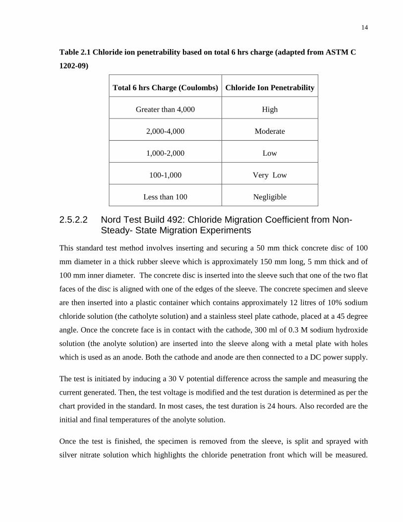
Table 2.1 Chloride ion penetrability based on total 6 hrs charge (adapted from ASTM C
1202-09)
Total 6 hrs Charge (Coulombs) Chloride Ion Penetrability
Greater than 4,000 High
2,000-4,000 Moderate
1,000-2,000 Low
100-1,000 Very Low
Less than 100 Negligible
2.5.2.2 Nord Test Build 492: Chloride Migration Coefficient from Non-Steady- State Migration Experiments
This standard test method involves inserting and securing a 50 mm thick concrete disc of 100
mm diameter in a thick rubber sleeve which is approximately 150 mm long, 5 mm thick and of
100 mm inner diameter. The concrete disc is inserted into the sleeve such that one of the two flat
faces of the disc is aligned with one of the edges of the sleeve. The concrete specimen and sleeve
are then inserted into a plastic container which contains approximately 12 litres of 10% sodium
chloride solution (the catholyte solution) and a stainless steel plate cathode, placed at a 45 degree
angle. Once the concrete face is in contact with the cathode, 300 ml of 0.3 M sodium hydroxide
solution (the anolyte solution) are inserted into the sleeve along with a metal plate with holes
which is used as an anode. Both the cathode and anode are then connected to a DC power supply.
The test is initiated by inducing a 30 V potential difference across the sample and measuring the
current generated. Then, the test voltage is modified and the test duration is determined as per the
chart provided in the standard. In most cases, the test duration is 24 hours. Also recorded are the
initial and final temperatures of the anolyte solution.
Once the test is finished, the specimen is removed from the sleeve, is split and sprayed with
silver nitrate solution which highlights the chloride penetration front which will be measured.

15
The chloride migration coefficient is determined using the following equation (NT Build 492-
99):
𝑫𝒏𝒔𝒔𝒎 =𝟎.𝟎𝟐𝟑𝟗(𝟐𝟕𝟑 + 𝑻)𝑳
(𝑼− 𝟐)𝒕�𝒙𝒅 − 𝟎.𝟎𝟐𝟑𝟖�
(𝟐𝟕𝟑 + 𝑻)𝑳𝒙𝒅𝑼 − 𝟐
� Eq. 2.17
Where, Dnssm is the non-steady-state migration coefficient, x10-12 m2/s, U is the absolute values
of the applied voltage, V, T is the average values of the initial and final temperatures in the
anolyte solution, °C, L is the thickness of the specimen, mm, xd is the average values of
penetration depths, mm and t is the test duration, hours.
2.6 Determining Diffusion Coefficient from Resistivity Measurements
It is also possible to calculate diffusion coefficients by determining the specific conductivity, σj,
of ionic species j through the concrete sample. The relationship between the diffusion coefficient
and the specific conductivity, σj, is described by the Nernst-Einstein equation (Andrade et al.,
1994; Lu, 1997; Stanish et al., 2001):
𝐷𝑗 =𝑅𝑇𝜎𝑗𝑧𝑗2𝐹2𝐶𝑗
Eq. 2.18
And the specific conductivity, σj, is defined as follows (Lu, 1997; Wright, 2007),
𝜎𝑗 = 𝑡𝑗𝜎 Eq. 2.19
Where, σ is the total conductivity and tj is the transport number of ionic species j.
According to Tong & Gjørv (2001), it is also possible to determine the diffusivity of a specific
aggressive ion into concrete via electrical conductivity measurements if both the conductivity
and diffusivity of the aggressive ion in the pore solution are known. This relationship is
formulated as follows (Tong & Gjørv, 2001):
𝜎𝜎0
=𝐷𝐷0
Eq. 2.20

16
Where, σ and D are the conductivity and diffusivity of the aggressive ion in the concrete and σ0
and D0 are the conductivity and diffusivity of the aggressive ion in the pore solution.
2.7 Ionic Movements Occurring During Electrical Migration Tests
2.7.1 Chloride Migration Tests
According to Andrade (1993), as soon as the water saturated concrete disc is exposed to both the
catholyte and anolyte and before any electrical potential is applied, ions begin to leach out of the
concrete specimens into the electrolytes and vice versa. In the case of rapid chloride migration
tests, where the catholyte and anolyte solutions are NaCl and NaOH, respectively, the following
ionic diffusions take place (Andrade, 1993):
1. OH- ions diffuse from the concrete specimen into the catholyte.
2. Cl- ions diffuse from the catholyte into the concrete specimen.
3. SO42- , K+ and Ca2+ ions diffuse from the concrete specimen into both solutions.
Also, due to their high ionic mobility, hydroxide ions are responsible for the majority of the
leaching (Andrade, 1993).
Andrade (1993) further explains that as soon as an electrical potential is applied to the system,
the following ionic migrations occur:
1. All anions migrate towards the anode, these include, Cl- from the catholyte, OH- and
SO42- from the concrete specimen and OH- from the anolyte.
2. All cations migrate towards the cathode, these include, Na+ from the anolyte, Na+, K+,
and Ca+2 form the concrete specimen and Na+ form the catholyte.
Therefore, during migration tests the applied electrical potential forces the migration of ions
through the cells and through the concrete specimen generating an electrical current and if at any
point during the test a concentration gradient is developed, the ionic migration will be
accompanied by ionic diffusion (Andrade, 1993; Wright, 2007).

17
The ionic movements occurring during chloride migration tests are summarized in Figure 2.1 to
Figure 2.3. Note that the middle section represents the concrete disc, the left section is the
catholyte and the right section is the anolyte.
Figure 2.1 Chloride migration tests: ionic movements due to diffusion. Adapted from
Andrade (1993).
Figure 2.2 Chloride migration tests: ionic movements due to migration. Adapted from
Andrade (1993).
Figure 2.3 Chloride migration tests: ionic movements due migration and diffusion.
Adapted from Andrade (1993).

18
2.7.2 Sulphate Migration Tests
In this study in addition to electrical chloride migration tests, electrical sulphate migration tests
were performed. Thus, it is reasonable to assume that similar processes as those discussed by
Andrade (1993) take place during sulphate migration tests where sodium sulphate solution rather
than sodium chloride is used. In the case of sulphate migration tests, the following ionic
movements occur due to diffusion initiating as soon as the water saturated sample is in contact
with the anolyte, NaOH, and catholyte, Na2SO4, but before applying an electrical potential:
1. OH- ions diffuse from the concrete specimen into the catholyte.
2. SO42- ions diffuse from the concrete specimen into the anolyte, under the assumption that
the concentration of SO42- in the catholyte is greater than that in the concrete, where the
majority of the SO42- present is in solid compounds rather than in the pore solution.
3. K+ and Ca2+ ions diffuse from the concrete specimen into both solutions.
Once an electrical potential is applied, the ion migrations occurring during the sulphate migration
tests are the same as those taking place during the chloride migration tests, but with sulphate ions
replacing chloride ions. As well, as mentioned above, the resultant ionic movements during a
migration test is the sum of ionic movements due diffusion and migration mechanisms. These
ionic movements, occurring during sulphate migration tests are summarized in Figure 2.4 to
Figure 2.6, note that the middle section represents the concrete disc, the left section is the
catholyte and the right section is the anolyte.
Figure 2.4 Sulphate migration tests: ionic movements under diffusion. Adapted from
Andrade (1993).

19
Figure 2.5 Sulphate migration tests: ionic movements under migration. Adapted from
Andrade (1993).
Figure 2.6 Sulphate migration tests: ionic movements under migration and diffusion.
Adapted from Andrade (1993).
2.8 Drawbacks of Non-Steady-State Electrical Migration Tests Electrical migrations tests, while are not as time consuming as diffusion tests, have several
drawbacks that should be acknowledged. During migration tests, the applied voltages induce
currents which if are high enough, heat up the system leading to a further increase in currents.
This issue is mainly encountered with the RCPT due to its high 60 V and mainly with poor
quality concrete. Higher currents due to heat generation increase the total charge passing leading
to conservative results (Andrade 1993; Liu and Beaudoin, 2000; Stanish et al., 2001; Samson et
al., 2003). The heating effect is not as significant in NT Build 492 test since the applied voltage
varies depending on the quality of the concrete. As well, in case the highest test voltage of 60 V
should be applied, heat generation will not have the same effect as that experienced with the
RCPT due to the significantly larger volume of the catholyte. Furthermore, in their paper,
Stanish et al., 2001, reference El-Belbol and Buenfeld’s (1989) tests done on 0.5 w/cm mortars,

20
in similar apparatus to that of the RCPT. Their findings showed that at 60 V, temperature rose by
18 °C while at 40 V temperature rise was considered “negligible”.
Both the RCPT and NT Build 492 are non-steady-state migration tests, where the flux of ions is
still increasing. For this reason, these tests are criticized for not representing either the diffusion
of aggressive ions into concrete or their chemical interactions that would occur in reality.
During the initial stages of migration tests, some of the penetrating ions reach chemically
reactive spots and become physically bound to the concrete, this chemical binding hinders the
movement of additional ions trying to penetrate into the concrete. Once all the chemically
reactive spots have been saturated with the penetrating ions, the flow (or current) of the
aggressive ion is no longer influenced by chemical binding (Andrade, 1993). Since chemical
binding influences ionic flow only in the initial stages of the exposure, it is the flow generated
after all chemical binding has taken place which is of interest. This subject leads to another
drawback of migration tests as according to Andrade (1993), the RCPT does not differentiate
between currents due to the flow of the aggressive ions while influenced by chemical binding
and flow of the aggressive ions after chemical binding has taken place. This is also the case for
NT Build 492, however, it should be acknowledged that determining the point at which chemical
binding no longer impacts ionic flow is very difficult and would complicate these migration tests
which are used specifically due to their simplicity and short test duration (especially the RCPT)
(Liu and Beaudoin, 2000; Stanish et al., 2001).
Another drawback mainly related to the RCPT is that the measured current during migration tests
is not only due to the flow of the aggressive ion being tested but rather due to the flow of all ions
present in the pore solution and in the electrolytes (Andrade 1993; Liu and Beaudoin, 2000;
Stanish et al., 2001; Samson et al., 2003).
To summarize, most of the drawbacks mentioned above are applicable to the RCPT, especially
since its results are based only on electrical conductivity measurements. NT Build 492 is less
problematic since the non-steady-state diffusion coefficient is evaluated directly using an
equation derived from the Nernst-Plank equation which requires the actual measurement of the
penetration front of the aggressive ion.

21
While both tests methods may not necessarily depict real rates of diffusion of aggressive ions
and their reactions with the concrete, the following points should be recognized:
1. In reality, with the exception of underwater concrete structures, the ingress of aggressive
ions into concrete is rarely only due to diffusion.
2. Diffusion coefficients obtained from NT Build 492 can be used to compare different
concretes.
3. Total charge values obtained from the RCPT can be used as an indication of concrete
quality. Moreover, Liu and Beaudoin, 2000, reported that Ozylidirim (1994), Berke
(1988) and Myers et al. (1997) found relatively good correlations between the RCPT,
effective diffusion coefficients and the long-term ponding test (AASHTO T259).
4. Since diffusion coefficients are used for direct comparisons of concrete, it is the relative
rather that the absolute diffusion coefficient which is of higher importance (Hooton,
2001). Therefore, it is essential that the diffusion coefficients are determined from the
same test methods and same equations.
5. Both tests are quick and simple (Liu & Beaudoin, 2000).
2.9 Conductance and Resistance
The current measured during migration tests such as the RCPT and NT Build 492 is the current
which is generated due to the movement of all ions present in both cell solutions and the concrete
pore solution. Thus, during RCPT for instance, the current generated due to the movement of
chloride ions represents a specific fraction of that total current. The fraction of current carried by
a specific ion is known as its transport number, represented by t+ and t- for the fractions of
cations and anions, respectively, and t++t-=1 (Wright, 2007). Transport numbers can be
calculated using the following equations (Wright, 2007):
𝑡+ =𝐼+𝐼𝑡𝑜𝑡𝑎𝑙
Eq. 2.21
And

22
𝑡− =𝐼−𝐼𝑡𝑜𝑡𝑎𝑙
Eq. 2.22
Where I+ and I- represent the current carried by the cation and anion respectively, and Itotal
represents the total current. Currents carried by the cations and anions can be evaluated using
equations derived from Ohm’s Law:
𝑅 =𝐸𝐼
Eq. 2.23
And
𝐺 =𝐼𝐸
Eq. 2.24
Where E is potential difference, R is resistance and G conductance. As can be observed
conductance is reciprocal to resistivity. According to Wright (2007), the resistance (or
conductivity) of a solid or a liquid is influenced by the chemical nature, homogeneity, size,
shape, and temperature. In the case of a solution, resistance (or conductivity) is also influenced
by the concentration of the ions present. The equations for resistance and conductance of a
sample uniform throughout its entire length are the following (Wright, 2007):
𝑅 = 𝜌𝑙𝐴
Eq. 2.25
And
𝐺 = 𝑘𝐴𝑙
Eq. 2.26
Where l is the length of the specimen, A is the area of the cross-section of the specimen, ρ is the
resistivity and k is the conductivity. Combining Ohm’s Law, Eq. 2.23, with Eq. 2.25 gives the
following equation (Wright, 2007):
𝐼 = 𝑘𝐸𝐴𝑙
Eq. 2.27

23
In an electrolyte, the total conductivity, ktotal, is the sum of the conductivities of the cations, k+
and the anions, k-, which in turn are defined as follows(Wright, 2007):
𝑘+ = 𝜆+𝑐+ Eq. 2.28
And
𝑘− = 𝜆−𝑐− Eq. 2.29
Where λ+ and λ- are the ionic molar conductivities of the cation and anion respectively, c+ and c-
are the concentration of the cation and anion respectively. It follows that (Wright, 2007):
𝑘𝑡𝑜𝑡𝑎𝑙 = Δ𝑐 Eq. 2.30
∴ Δ = 𝜆+ + 𝜆− Eq. 2.31
Eq. 2.31, formulates Kohlrausch’s Law of independent ionic migration which states that “each
ion contributes a definite amount to the total molar conductivity of the electrolyte irrespective of
the nature of the electrolyte” (Wright, 2007, p. 443) Using Eq. 2.27 to Eq. 2.30, the transport
number equations, Eq. 2.21and Eq. 2.22, can be re-written as follows (Wright, 2007):
𝑡+ =𝑘+𝑘�𝐸𝐴𝑙� �
𝑙𝐸𝐴
� =𝑘+𝑘
=𝜆+𝑐+Δ𝑐
Eq. 2.32
And
𝑡− =𝑘−𝑘�𝐸𝐴𝑙� �
𝑙𝐸𝐴
� =𝑘−𝑘
=𝜆−𝑐−Δ𝑐
Eq. 2.33
Therefore, according to Eq. 2.32 and Eq. 2.33, the contribution of a specific ion to the measured
currents depends on both on its concentration and its molar conductivity. However, in the case of
concrete pore solution where the ionic strength is high, Andrade (1993) suggests considering
ionic activities rather than concentration. Ideally, during migration tests, the transport number of
the aggressive ionic species tested would be calculated to determine the current generated due to
the movement of the aggressive ions only (Andrade, 1993).

24
2.10 Variables Affecting Test Results While conductivity measurements are primarily influenced by pore solution conductivity and
electrolyte conductivity, diffusions rates are influenced by both the pore solution and the
capillary pore structure of the concrete (Stanish et al., 2001). It is therefore imperative to review
both the material variables which influence the continuity and size of the capillary pore structure
(Ann et al., 2009) as well as the variables affecting conductivity.
2.10.1 Electrical Conductivities of NaCl and Na2SO4 Electrolytes and Cl- and SO4
2- Ions
During the migration tests conducted in this study, the resistance of concrete to the penetration of
chloride was measured using NaCl solution while the sulphate penetration resistance was
measured using Na2SO4 solution. The chloride and sulphate migration tests were conducted on
concrete specimens cut from the same cylinder in order to have a better comparison of the test
results. Thus, to accurately compare how resistant concrete is to the penetration of chloride as
opposed to sulphate, it is important to take into consideration how the nature of the electrolytes
used will affect conductivity measurements and, therefore, the test results. The electrical
conductivities of NaCl and Na2SO4 solutions at concentrations relevant to the migration tests
conducted in this study are presented in Table 2.2. As can be seen, NaCl is more conductive than
Na2SO4 and the difference increases with increased concentration. Therefore, it is reasonable to
expect higher currents (and thus higher total charge values) in both RCPT and NT Build 492
tests for concrete specimens exposed to chlorides than those exposed to sulphates.

25
Table 2.2 Electrical conductivity values of NaCl and Na2SO4 solutions at 2, 5 and 10%
concentrations at 20°C obtained from the “CRC Handbook of Chemistry and Physics”,
Haynes & Lide, 2011.
Concentration, mass %
Electrical Conductivity, k, mS/cm (S=Ω-1)
Relevant Test
Method Electrolyte
NaCl Na2SO4
2 % 30.2 19.8 RCPT (done at 3%)
5% 70.1 42.7 -
10% 126 71.3 NT Build 492
Similarly, assuming identical concrete specimens are tested in chloride and sulphate migration
tests, to produce a more accurate comparison of the penetration of chlorides and sulphates, it is
important to compare their ionic conductivities and transport numbers. The conductivities and
diffusion coefficients at infinite dilution of chloride and sulphate are presented in Table 2.3.
Assuming identical concrete specimens are tested in the same migration tests, taking into
consideration the diffusion coefficient data presented in Table 2.3 and recognizing that the
sulphate ion is larger than the chloride ion, it is expected that the specimens exposed to sulphate
would have lower diffusion coefficients and lower penetration depths than the specimens
exposed to chloride. Maintaining the assumption that identical specimens are tested in the same
migration tests, from the molar conductivity data presented in Table 2.3 and from the equations
presented in Section 2.9, it may be inferred that for the same current value, the contribution of
sulphate to the total current measured across the sulphate-exposed specimen is greater than the
contribution of chloride to the total current measured across the chloride-exposed specimen.

26
Table 2.3 Conductivities and diffusion coefficients at infinite dilution of chloride, sulphate
and additional common ionic species present in the pore solution obtained from the “CRC
Handbook of Chemistry and Physics”, Haynes & Lide, 2011.
Ion
Molar Conductivity, at
infinite dilution, λ°
10-4 m2 S mol-1
Diffusion Coefficient, D, in
dilute aqueous solution
10-9 m2/s
Cl- 76.3 2.032
SO42- 160.0 1.065
OH- 197.6 5.273
Na+ 50.1 1.334
K+ 73.5 1.957
Ca2+ 119.0 0.792
2.10.2 Effects of Degree of Hydration and Water to Cement/Binder Ratio
Ingress of aggressive ions into concrete is accomplished via the concrete’s capillary pore system.
Higher continuity of capillary pores and larger pores facilitate fluid ingress into the concrete
leading to higher diffusion rates. It is well known that water-cement (w/cm) ratio has a great
impact on the capillary pores, as the w/cm ratio decreases, capillary porosity volume decreases
and becomes more discontinuous (Powers & Brownyard, 1946; Mehta and Monteiro, 2006; Han,
2007). Therefore, as w/cm (or w/b) ratio decreases, diffusion coefficient decreases (Mehta and
Monteiro, 2006; Chalee & Jaturapitakkul, 2009).
The continuity and size of the capillary pore system are also influenced by the degree of
hydration of the cementing materials in concrete. Greater degree of hydration reduces the size
and continuity of the capillary pores (Powers & Brownyard, 1946; Mehta & Monteiro, 2006),
leading to reduction in diffusion rates. As long as sufficient moisture is available, the degree of
hydration of the cementing materials in concrete will increase with age. The change in size and

27
continuity of the capillary pore system are the greatest at early age when the number of largest
pores are reduced (Mehta & Monteiro, 2006).
2.10.3 Effects of Supplementary Cementing Materials
The continuity and size of the capillary porosity are also influenced by the addition of
supplementary cementing materials (SCMs). SCMs react with calcium hydroxide and water to
form secondary lower density C-S-H. This reaction modifies the capillary pores as larger pores
are filled with “microporous, low density material”, leading to the reduction in the size of the
capillary pores. This process is known as “pore-size refinement” (Mehta and Monteiro, 2006).
Moreover, the capillary porosity further deceases due to the replacement of the relatively large
size of the calcium hydroxide crystals with several smaller crystals and secondary hydration
products. This process is known as “grain-size refinement” (Mehta and Monteiro, 2006).
Various sources reported a decrease in the chloride diffusion coefficient upon the addition of
SCMs to the concrete (Hooton, 2001; Julio-Betancourt 2002; Thomas & Matthews, 2004;
Nokken et al., 2006; Oh & Jang, 2007; Chalee & Jaturapitakkul, 2009). This effect was expected
as it is known that SCMs increase the density of the concrete due to the formation of secondary
C-S-H, making it less permeable with time, thereby reducing diffusion (Chalee & Jaturapitakkul,
2009).
The influence of SCMs on diffusion varied depending on the percent replacement of cement, the
age of the concrete and the fineness of the SCM. According to Thomas and Matthews (2004),
after 4 years of marine exposure, concrete with the highest fly ash replacement had the lowest
chloride threshold concentrations and chloride concentrations increased as fly ash replacement
decreased. Furthermore, following 10 year exposure, chloride content in the 21-26 mm depth
interval of a 100% Portland cement concrete was 3.50% (by mass of cement), whereas for the
same interval, a 50% fly ash concrete chloride content was only 0.42%. According to Julio-
Betancourt (2002), the effect of SCMs is more pronounced as concrete ages. The use of finer
SCMs reduces diffusion, in the case of fly ash, the reduction in chloride diffusion coefficient due
to addition of finer fly ash was found to be more effective for concrete with higher w/b ratios
(Chalee & Jaturapitakkul, 2009).

28
According to Chalee and Jaturapitakkul (2009) and Han (2007), reduction in w/cm ratio is more
effective in reducing diffusion coefficient than addition of SCMs, making w/cm the most
influential material parameter.
2.10.3.1 Effect of Slag Replacement on Sulphate Attack
Although replacing a portion of the cement with slag reduces the size and continuity of the
capillary porosity, it should be noted that slag also contributed reactive alumina which in turn
influences sulphate attack. According to Mehta and Monteiro (2006), studies done to investigate
the effect of slag replacement on sulphate attack in concrete indicated the followings:
1. The use of 60 -65% slag replacement showed high sulphate resistance regardless of the
alumina content of the slag.
2. The use of low alumina content slag (11%) increased concrete’s resistance to sulphate
attack regardless of the alumina content of the cement.
3. The use of high alumina content slag (18%) in less than 50% replacement increased the
susceptibility of the concrete to sulphate attack.
2.10.4 Effect of Cement Type
Both chlorides and sulphates chemically react with the hydration products of the tricalcium
aluminate, C3A, in the cement (Mehta and Monteiro, 2006). The greater the C3A content the
greater the potential for these chemical reactions to occur. Therefore, the amount of chemical
reactions (or binding) occurring the concrete will primarily depend on the C3A content in cement
type used. GU cement with the highest C3A content, will have the highest amount of chemical
binding, followed by MS cement and finally by HS cement.
Therefore, since chloride binding involves the physical binding of chloride ions to the concrete,
the movement of additional chloride ions through the bound chloride layer is hindered, resulting
in a lower amount of electrical charge passing through the specimen, smaller penetration depths
and lower diffusion coefficients.
Oh and Jang (2007) found that apparent chloride diffusion coefficient varied depending on the
cement type that was used. Apparent chloride diffusion coefficients for Type I (GU) cements
were found to be smaller than those of Type V (HS) cements. The reason for this variance
originates from the fact that Type V (HS) cement contains less C3A, which increases the binding

29
capacity of concrete. That is, cements with higher C3A contents result in more chloride binding
which decreases the apparent chloride diffusion coefficient (Han, 2007).
2.10.4.1 Effect of Cement Type on the Degree of Hydration
The degree of hydration of cement directly impacts the porosity and permeability of concrete,
such that concretes with higher degree of hydration are stronger and more durable (Mehta &
Monteiro, 2006). Other than being time-dependent, the degree of hydration is also influenced by
the phase composition of the different cement types, primarily Alite, C3S, and Belite, C2S. The
hydration reactions of C3S and C2S are the following (Mehta & Monteiro, 2006):
2𝐶3𝑆 + 6𝐻 → 𝐶3𝑆2𝐻3 + 3𝐶𝐻 Eq. 2.34
2𝐶2𝑆 + 4𝐻 → 𝐶3𝑆2𝐻3 + 𝐶𝐻 Eq. 2.35
Thus, the products of hydration of C3S are 61% C-S-H and 39% CH and those of the C2S
hydration are 82% C-S-H and 18% CH. Taking this in consideration and acknowledging that the
properties of cement paste are attributed to the formation of C-S-H, it may be inferred that
cements with high C3S content will be weaker than cements with high C2S content. (Mehta &
Monteiro, 2006) In addition, according to Mehta and Monteiro (2006), the presence of CH
reduces the durability of the hardened cement paste to sulphate and acidic waters. Therefore,
cements with higher contents of C2S will be more durable than cement with higher contents of
C3S. With respect to the rate of reaction, Mehta and Monteiro (2006) state that C3S reacts faster
than C2S, and therefore C3S is responsible for the early strength gain and C2S is responsible for
the long term strength gain.
It follows then, that the GU cement with higher C2S and lower C3S contents than the MS and HS
cements would be more durable and stronger in the long run. Whereas, the MS and HS cements
of would have higher early strengths and higher degree of hydration up to 28 days (Mehta &
Monteiro, 2006).
2.10.5 Effect of Chemical Binding
As mentioned earlier, a portion of the chloride ions entering the concrete will chemically react
with C3A and C4AF to produce physically bound chlorides known as Friedel’s salt (Zibara, 2001;
Han 2007). These physically bound chlorides hinder the movement of the remaining free

30
chlorides through the concrete, thereby reducing diffusion rate. Thus, chloride binding reduces
apparent diffusion coefficients and concrete with higher chloride binding capacity was found to
reduce chloride diffusivity to a greater extent (Zibara, 2001; Oh & Jang, 2007). Concrete binding
capacity is governed by content of C3A, according to Han (2007), concrete containing 14% C3A
was found to have twice as much bound chloride as concrete containing 2% C3A. However,
larger amounts had less effect (Han, 2007). According to Oh and Jang (2007), chloride binding
capacity has the greatest effect near the surface exposed to chlorides. Since C3A also reacts with
sulphates, it is reasonable to assume that migration test results will be influenced more by
concretes containing cements with higher C3A contents. However, more research is necessary to
investigate the nature of sulphates binding during initial exposure periods as those occurring
during the rapid sulphate migration tests.

31
Chapter 3 Experimental Procedure
3
3.1 Materials Nine concrete mixtures of varying water to cementitious materials ratios, cement types and slag
replacements were tested in this program to investigate their influence on test results.
3.1.1 Cementitious Material
Type GU, general use, Portland Cement from Holcim’s Mississauga cement plant was used in
four of the nine concrete mixtures. High-sulphate-resistant, HS, cement from Lehigh Inland’s
Edmonton plant was used in two of the nine mixtures. From the same plant, Lehigh Inland’s
Type GU cement was also used in two of the nine mixtures. Lehigh Inland’s Type GU cement is
produced to meet the requirements of Western Canadian construction industry, where the levels
of sulphates in soils are relatively high. Thus, in this paper, Lehigh Inland’s Type GU cement
was referred to as Type MS, moderate-sulphate-resistant, cement as its C3A content is less than
8%. Also from same Edmonton plant, Lehigh Inland’s InterCemTM, GUb-30F, which is blended
Type GU blended cement with 30% Class F fly ash, this cement type was used in only one of the
nine concrete mixtures (Lehigh Inland Cement Limited, 2011). All cement types used meet the
CSA A3001 requirements for their specific type. Chemical analyses of the cements are presented
in Table 3.1.
3.1.2 Blast-Furnace Slag
Ground Granulated Blast-Furnace Slag conforming to CSA A3001 requirements from Lafarge’s
Stoney Creek plant was used as cement replacement in four of the nine mixtures. Three of these
mixtures contained slag from the same production date and the fourth mix contained slag from
another production date. Chemical analyses of the slag used are shown in Table 3.1.

32
Table 3.1 Chemical and mineralogical compositions
* In this paper, Lehigh Inland Type GU cement is referred to as Type MS cement.
Component
(%)
Holcim GU
Cement
Lehigh
Inland
GU*
Cement
Lehigh
Inland
HS Cement
Lehigh
Inland
InterCemTM
GUb-30F
Lafarge
Stoney
Creek
Blast-
Furnace
Slag #1**
Lafarge
Stoney
Creek
Blast-
Furnace
Slag #2***
SiO2 19.78 20.33 20.51 28.37 34.95 37.24
Al2O3 5.43 4.48 3.92 10.49 10.71 8.70
Fe2O3 2.16 3.76 4.65 4.36 0.51 0.35
CaO 61.59 63.09 61.64 49.63 35.88 37.94
MgO 2.36 2.84 3.05 2.50 11.68 11.36
SO3 4.06 2.79 2.55 2.48 1.35 1.07
K2O 1.23 0.514 0.566 0.702 0.52 0.43
Na2O 0.250 0.237 0.219 0.843 0.36 0.43
TiO2 0.267 0.167 0.153 0.345 0.73 0.48
SrO 0.080 0.047 0.044 0.069 - _
P2O5 0.125 0.026 0.024 0.030 - 0.02
Cl 0.016 0.003 0.003 0.003 - 0.01
ZnO 0.007 0.014 0.019 0.014 - _
Cr2O3 0.008 0.004 0.007 0.009 - 0.11
Mn2O3 0.059 0.029 0.027 0.039 0.78 0.46
Leco CO2 1.65 - - - - 0.38
Leco SO3 _ - - - - 0.864
Free lime 0.66 - - - - -
LOI 1000℃ 2.26 - - - - -0.15
LOI 750℃ - - - - - 0.83
Blaine
(m2/kg) 416 415 439 514 448 -
Mineralogical Composition
Bogue C3A 10.74 5.51 2.51
Bogue C2S 27.98 13.86 17.42

33
** Slag #1 was used in all 3 of the slag containing Holcim Type GU mixtures. *** Slag #2 was used in the only slag containing mixture of Type MS.
3.1.3 Fine Aggregate
Fine aggregate used was natural sand from Dufferin Aggregates’ (Holcim’s) Mill Creek pit in
Cambridge. Physical properties of the sand are presented in Table 3.2.
3.1.4 Coarse Aggregate
Coarse aggregate used was Niagara escarpment crushed dolomitic limestone from Dufferin
Aggregates’ Milton quarry. Physical properties of the coarse aggregate are presented in Table
3.2.
Table 3.2 Physical properties of the fine and coarse aggregates
Property Fine Aggregate Coarse Aggregate
Nominal Maximum Size (mm) - 20
Fineness Modulus 2.81 -
Relative Density (SSD)
(kg/m3) 2,678 2,677
Relative Density (OD) (kg/m3) 2,707 2,715
Apparent Relative Density
(kg/m3) 2,756 2,784
Absorption (%) 1.06 1.44
* Calculations of these properties are available in Appendix A.
3.1.5 Chemical Admixtures
The only chemical admixture added to the mixture was Glenium 7700, a high-range water
reducer manufactured by BASF Construction Chemicals.

34
3.1.6 Water
The water used in the mixtures was tap water from the City of Toronto.
3.2 Mix Designs Since the main goal of this study is to develop a rapid test method to evaluate the penetrability of
sulphate ion into concrete, it was reasonable to select mix designs which conform to the CSA
A23.1-09 requirements for concrete in various levels of sulphate, S, exposure. All the selected
mix designs conform to the minimum requirements in Table 2 of the CSA A23.1-09, where the
maximum water to cement ratios are 0.40, 0.45, and 0.5 for S-1 (very severe), S-2 (severe) and
S-3 (moderate) exposures, respectively. Moreover, all the mix designs containing HS and MS
cements conform with the additional requirements for concrete subjected to sulphate attack,
presented in Table 3 in the CSA A23.1-09 standard.
3.2.1 Mix Proportions
All nine mixtures were proportioned using the Absolute Volume method presented in the Design
and Control of Concrete Mixtures book (Kosmatka et al., 2003). Mix proportions are presented
in Table 3.3.

35
Table 3.3 Mix proportions per 1 m3
Materials
(Kg)
Mix Properties
w/cm
Cement Type
% Slag replacement
0.5
GU
0%
0.5
GU
35%
0.45
GU
50%
0.4
GU
50%
0.5
InterCem
GUb-30F
0%
0.45
HS
0%
0.4
HS
0%
0.5
MS
0%
0.4
MS
50%
Cement 214.5 330.0 183.3 206.3 330.0 366.7 412.5 330.0 206.3
Slag 115.5 0.0 183.3 206.3 0.0 0.0 0.0 0.0 206.3
Coarse
Aggregate 962.7 962.7 962.7 962.7 962.7 962.7 962.7 962.7 962.7
Fine
Aggregate 930.5 938.9 894.3 853.7 938.9 907.8 868.8 938.9 853.7
Water 165.0 165.0 165.0 165.0 165.0 165.0 165.0 165.0 165.0
3.2.2 Casting
The materials for each mix were all weighed and kept in sealed plastic buckets 1 day prior to
casting. The moisture contents of the sand and coarse aggregate were determined as per ASTM C
70 and C 566, respectively, and mix designs were adjusted accordingly. Prior to determining the
moisture content of the coarse aggregate, the stone was washed, spread across a metal pan to dry
uniformly and then moved to plastic buckets which were then sealed. A concrete mixer of 18
litre capacity was used to batch the concrete. Prior to the addition of the materials to the mixer,
the mixer was moistened with a wet rag, then, the sand, cement and coarse aggregate were added
to mixer, respectively. The sand, cement and coarse aggregate were all mixed for 1 minute after
which the water with the water reducer dispersed in it, was added to the mixer. The materials
were then mixed for 3 minutes, rested for 3 minutes and then mixed once again for 2 minutes
(ASTM C192/C 192M - 07). Once the mixing was done, the slump and fresh density were
determined for control purposes, as per ASTM C143/C143M – 08 and C 138/C 138M – 08. A
slump of 60-120 mm was targeted.

36
The concrete was then placed in ten 100x200 mm plastic cylinder moulds, which were prepared
1 day prior to casting. Each plastic cylinder mould was filled with 3 layers of concrete of
approximately equal volumes. The cylinders were consolidated by rodding as indicated in
Section 7.4.2 in ASTM C 192/C 192M – 07.
Taking into consideration the quantity of samples which may be tested in the electrical migration
tests per day, it was decided to cast only one or two mixtures per week. When two mixtures were
cast per week, they were cast 1 day apart.
3.2.3 Curing
Following casting, the concrete cylinders were capped and placed in a moist cure room (100%
relative humidity at 23°C). All concrete cylinders were demolded the next day, labelled and
placed back in the moist room until test.
3.3 Test Procedures As previously mentioned, ten cylinders were cast per mix. Due to the limited number of
cylinders, compressive strength tests were done on two of these cylinders, one at of 7 and 28
days. Electrical migration and resistivity tests were performed on the remaining eight cylinders,
four cylinders were tested at 35 days and the other four cylinders were tested at 56 days. Each
cylinder was saw-cut into four slices such that the middle two sections were approximately 50
mm thick, resulting in two, 100 mm in diameter and 50 mm thick, concrete discs per cylinder.
Therefore, at each test date (35 and 56 days) a total of eight concrete discs were tested per mix.
Figure 3.1 shows a schematic of the four cylinders tested per test date along with labelling of the
test and exposure solution that each sample was subjected to. The arrows in Figure 3.1 indicate
the face of the sample that was exposed to the aggressive ions.

37
Figure 3.1 Schematic of the test plan at each migration test date
As mentioned in Chapter 2, two standard migration tests were performed in this study,
1. ASTM C 1202 (Rapid Chloride Permeability Test, RCPT), Electrical Indication of
Concrete’s Ability to Resist Chloride Ion Penetration
2. Nord Test NT Build 492, Chloride Migration Coefficient from Non-Steady-State
Migration Experiments
Both of these standard tests were also modified by exposure to sulphate, rather than chloride
ions. As may be inferred from Figure 3.1, the specimens were divided such that an equal number
of specimens were tested in the both original standard tests with chloride exposure and both
modified tests with sulphate exposure. The original and modified tests ran in parallel to each
other, and both the ASTM C 1202 and the NT Build 492 tests were conducted on the same test
day. The next section discusses in detail the modified tests.
Note that for both migration tests, the concentrations of the catholyte solutions were not
modified. Therefore, for the same catholyte concentration (by mass), there were 2.4 times more
moles of chloride than sulphate ions available in the catholyte solution:

38
𝑚𝑜𝑙𝑎𝑟 𝑚𝑎𝑠𝑠𝑒𝑠: 𝑁𝑎𝐶𝑙 = 58.44𝑔𝑚𝑜𝑙
;𝑁𝑎2𝑆𝑂4 = 142.04𝑔𝑚𝑜𝑙
;
1 𝑚𝑜𝑙 𝑜𝑓 𝑁𝑎𝐶𝑙 → 1 𝑚𝑜𝑙 𝑜𝑓 𝐶𝑙−; 1 𝑚𝑜𝑙 𝑜𝑓 𝑁𝑎2𝑆𝑂4 → 1 𝑚𝑜𝑙 𝑜𝑓 𝑆𝑂42−, 𝑡ℎ𝑢𝑠:
1 𝑔 𝑜𝑓 𝑁𝑎𝐶𝑙 ∙1 𝑚𝑜𝑙
58.44 𝑔= 0.017 𝑚𝑜𝑙𝑒𝑠 𝑜𝑓 𝑁𝑎𝐶𝑙 𝑜𝑟 0.017 𝑚𝑜𝑙𝑒𝑠 𝑜𝑓 𝐶𝑙−.
1 𝑔 𝑜𝑓 𝑁𝑎2𝑆𝑂4 ∙1 𝑚𝑜𝑙
142.04 𝑔= 0.007𝑚𝑜𝑙𝑒𝑠 𝑜𝑓 𝑁𝑎2𝑆𝑂4 𝑜𝑟 0.007 𝑚𝑜𝑙𝑒𝑠 𝑜𝑓 𝑆𝑂42−.
0.017 𝑚𝑜𝑙𝑒𝑠 𝑜𝑓 𝐶𝑙−
0.007 𝑚𝑜𝑙𝑒𝑠 𝑜𝑓 𝑆𝑂42−= 2.4
It is probable that this difference in the number of moles of chloride and sulphate ions available
in the catholyte solutions would influence the results of the migration tests (higher chloride
penetrations would be expected). However, chloride and sulphate penetration resistances may be
influenced to a greater extent by other differences, such as their molecular size, diffusivity in
dilute aqueous solution, and molar conductivities. The influence of the molecular size and
diffusivity differences would vary depending on the size and continuity of the capillary pore
system. If sulphates cannot enter the concrete due to the size of the capillary pores, the amount of
sulphate ions available to penetrate would not be as significant as the size of the capillary pores.
3.3.1 Modification of ASTM C1202
Only a single modification was made to ASTM C 1202 to evaluate concrete’s resistance to the
penetration of sulphate ions by measurements of electrical conductance. Instead of using 3%
sodium chloride solution as the catholyte, 3% sodium sulphate solution was used.
Other than this modification, the accelerated sulphate tests were conducted exactly as the
accelerated chloride tests. Therefore, please refer to ASTM C 1202 standard and to the sections
below which discuss slight modifications in the conditioning of the samples and the test
procedure (for both the sulphate and chloride tests).
Note that a similar modification of the rapid chloride permeability test into a rapid sulphate
permeability test was done previously by Tumidajski and Turc in 1995.

39
3.3.1.1 Conditioning Modification
Since all the specimens tested were cured in a moist room with 100% relative humidity until test,
it was reasonable to assume that the capillary pore system was in great part saturated with water
rather than air. Nonetheless, the specimens were vacuum saturated as follows. Specimens were
placed in vacuum desiccators that were then filled with tap water such that all the specimens
were completely submerged under water. When multiple specimens were placed in the same
container, it was ensured that the cut faces of each specimen were exposed. The vacuum
desiccators were then sealed and the vacuum pump was started. The specimens remained under
vacuum for 3 hours. Following vacuum saturation, air was let in, Merlin and Monfore electrical
resistivities were measured and then specimens were returned to the water filled containers were
they remained immersed for 18± 2 hours. Thus, all specimens were vacuum saturated 1 day
prior to their planned test date. That is, at 34 and 55 days, and were sawn cut several days earlier.
3.3.1.2 Procedure Modification
In this study, all the steps mentioned in the procedure section in ASTM C 1202 were performed,
in addition to the following steps.
1. Once excess water was blotted off, the curved sides of the specimens were wrapped with
vinyl electrical tape.
2. Once the test had started, the current, temperature and coulombs passed were recorded
manually for each specimen at 1 and 5 minutes into the test, to enable the calculation of
the electrical resistivity of the specimens.
3. At the end of the 6 hour accelerated test, the specimens exposed to chlorides were split
and sprayed with silver nitrate to determine the chloride front, as done in NT Build 492.
The specimens exposed to sulphate were not split since sulphates were not expected to
penetrate to measurable depths after 6 hours exposure to 60 volts.
3.3.1.3 Interpretation of Results
A table which qualitatively ranks the sulphate ion penetrability resistance of the specimens based
on the total amount of charge passed is developed in Chapter 4 (see Table 4.8).

40
3.3.2 Modification of NT Build 492
In addition to modifying the catholyte solution from 10% sodium chloride to 10% sodium
sulphate, to identify the sulphate front it was necessary to use a colorimetric method different
than spraying silver nitrate (which identifies chlorides). The colorimetric method used to identify
sulphates involved ponding barium chloride, potassium permanganate solution onto the split
sulphate exposed specimen using a glass dropper, it is explained in further detail in Sections
3.3.2.3 and 3.3.2.4.
Apart from than these modifications, the accelerated sulphate tests were conducted the same as
for the accelerated chloride tests. Refer to NT Build 492 and to the sections below which discuss
slight modifications to the preconditioning of the samples and test preparation (for both the
sulphate and chloride tests).
3.3.2.1 Preconditioning Modifications
Once the specimens were surface dry, they were placed in a vacuum container and saturated
Ca(OH)2 was added such that the specimen were completely submerged. Ensuring that the
surfaces were exposed, the specimens were vacuum treated for 3 hours. Once the vacuum
saturation was complete, air was let it, Monfore and Merlin electrical resistivities were measured
and the specimens were placed back in solution where they remained soaked for 18 ± 2 hours.
Thus, all specimens were vacuum saturated 1 day prior to their planned test dates. That is, at 34
and 55 days, and were sawn cut several days earlier.
3.3.2.2 Test Preparation Modification
Two specimens, rather than one, were placed in the each of the (approximately) 12 litres sodium
chloride and sodium sulphate catholyte reservoirs. Figure 3.2 shows the circuit diagram of the
test set up. Note that the DC power supply used was an HP E3612A which has digital voltage
and current meters, with current displayed to the nearest mA. From Figure 3.2, it may be
observed that the specimens were connected in parallel and therefore the same voltage was
applied to each specimen. Since a series connection follows the parallel connection, the current
displayed on the digital ammeter on the DC potential display was the sum of the currents going
through both specimens. To measure the current passing through each specimen, the anode of the
other specimen was momentarily removed from the NaOH solution.

41
Figure 3.2 Circuit diagram of the NT Build 492 test set-up used in this study
3.3.2.3 Sulphate Staining Overview
In order to determine the depth of sulphate ion penetration, sulphates were stained by ponding
barium chloride, potassium permanganate solution onto the specimen using a glass dropper.
A fundamental test for the presence of sulphates involves the addition of Ba3+ (usually from
BaCl2) to a solution consisting of SO42- and the precipitation of white barium sulphate. A
distinctive purple stain of the barium sulphate can be achieved by the addition of potassium
permanganate to the original SO42- solution (Poole & Thomas, 1975).
The staining procedure according to Poole and Thomas (1975) involves preparing a 6% mixed
barium chloride and potassium permanganate solution in which the specimen is immersed for 2
minutes. The specimen is then washed in a saturated solution of oxalic acid to remove coloration
due to excess permanganate. With respect to the colour intensity, the optimal ratio for the
solution was found to be 2:1 barium chloride to potassium permanganate (Poole & Thomas,
1975).
Poole and Thomas further determined that a sample immersed in a 6% solution reached
maximum colour intensity after two minutes and the minimum shelf life of the solution is 6
weeks as long as the solution is kept in a brown glass bottle.

42
Therefore, in this study, 6% barium chloride, potassium permanganate solution was prepared to
stain and identify the sulphate front, with a 2:1 barium chloride to potassium permanganate ratio.
To make 100 ml of solution, 97.83 grams of water were mixed with 4 grams of barium chloride
and 2 grams of potassium permanganate.
3.3.2.4 Sulphate Front Staining Procedure
Once the migration test was completed and the specimen was split, the following steps were
carried out to identify the sulphate front.
Step 1: While keeping the split face of the specimen facing upwards in a container, distilled
water was sprayed lightly on the split face to put the sulphates in solution.
Step 2: using a glass Pasteur pipette with a bulb (a glass dropper) and while wearing a protective
mask and gloves, small quantities of the dye were ponded onto the split face (which was kept
facing upwards throughout), and were left on for 3 minutes after which the stain was washed
away using distilled water, saturated oxalic acid and distilled water again to remove excess
oxalic acid which otherwise leaves white precipitate when dried.
Step 3: Excess distilled water was blotted off the sample using paper towels and the diluted
barium chloride potassium permanganate solution in the container was placed in a chemical
waste container.
Step 4: Approximately 20 minutes after step 3 was completed, the samples were dry enough to
measure the sulphate front.
The measured sulphate fronts of the NT Build 492 specimens were typically only several mm
deep. Therefore, in some cases the sulphate front was measured to the nearest 0.25 of a mm by
comparing the front depth to a line width chart. The sulphate front otherwise, was measured in
exactly the same manner as the chloride penetration front which is described in NT Build 492.
3.3.2.5 Calculating the Sulphate Migration Coefficients
The equation given in NT Build 492 for the calculation of the migration coefficient is the
following:

43
𝐷𝑛𝑠𝑠𝑚 =𝑅𝑇𝑧𝐹𝐸
∙𝑥𝑑 − 𝛼�𝑥𝑑
𝑡 Eq. 3.1
Where:
𝐸 =𝑈 − 2𝐿
Eq. 3.2
𝛼 = 2�𝑅𝑇𝑧𝐹𝐸
∙ 𝑒𝑟𝑓−1 �1 −2𝑐𝑑𝑐0� Eq. 3.3
And Dnssm is the non-steady-state migration coefficient, m2/s; z is the absolute value of ion
valence for chloride and sulphate z = 1 and z = 2, respectively; F is the Faraday constant,
F=9.648x10⁴ J/(V∙mol); U is the absolute values of the applied voltage, V; R is the gas constant,
R=8.314 J/(K∙mol); T is the average value of the initial and final temperatures in the anolyte
solution, K; L is the thickness of the specimen, m; Xd is the average values of penetration depths,
m; t is the test duration, seconds; erf-1 is the inverse of error function; cd is the chloride
concentration at which the colour changes, cd≈ 0.07 N and C0 is the chloride concentration in
the catholyte solution, c0≈ 2 N.
As may be observed, due to the terms, cd and c0, the equation above becomes specific to the
calculation of the chloride migration coefficient. For the calculation of the sulphate migration
coefficient, the sulphate concentration in the catholyte solution, C0, was calculated to be 0.704
moles as follows:
10% Na2SO4 solution, 100g of Na2SO4 added to 980g of H2O, molar mass of Na2SO4 = 142.042
g/mol,
𝑚𝑜𝑙𝑒𝑠 𝑜𝑓 𝑁𝑎2𝑆𝑂4 = 𝑚𝑎𝑠𝑠 𝑜𝑓𝑁𝑎2𝑆𝑂4(𝑔)
𝑚𝑜𝑙𝑎𝑟 𝑚𝑎𝑠𝑠 𝑜𝑓 𝑁𝑎2𝑆𝑂4 � 𝑔𝑚𝑜𝑙�
= 100 𝑔𝑟𝑎𝑚𝑠 𝑜𝑓𝑁𝑎2𝑆𝑂4142.042 𝑔
𝑚𝑜𝑙=
0.704 𝑚𝑜𝑙𝑒𝑠 𝑜𝑓 𝑁𝑎2𝑆𝑂4; 1 𝑚𝑜𝑙𝑒 𝑜𝑓 𝑁𝑎2𝑆𝑂4 = 1 𝑚𝑜𝑙 𝑜𝑓 𝑆𝑂4
∴ 𝑠𝑢𝑙𝑝ℎ𝑎𝑡𝑒 𝑐𝑜𝑛𝑐𝑒𝑛𝑡𝑟𝑎𝑡𝑖𝑜𝑛 𝑖𝑛 𝑡ℎ𝑒 𝑐𝑎𝑡ℎ𝑜𝑙𝑦𝑡𝑒 𝑠𝑜𝑙𝑡𝑢𝑖𝑜𝑛, 𝑐0 = 0.704 𝑚𝑜𝑙𝑒𝑠
The determination of the sulphate concentration at which the colour changes, cd, is more
complex than that of the catholyte solution and is beyond the scope of this study. However, it

44
was possible to roughly estimate the sulphate concentration at which the colour changes using
ICP results obtained from acid digested solutions of concrete powders belonging to two profile
ground sulphate exposed specimens. This is a very rough estimation due to the following
reasons:
1. ICP results represent the total sulphur present per unit weight of ground concrete,
however, it is the sulphate content that is of interest. Therefore, the assumption is that all
the sulphur present is from sulphate (although, since slag contains sulphur, this
assumption may not be as accurate for the specimen that contained slag).
2. It is also assumed that all the “sulphates” measured by ICP are soluble (not physically
bound), although, ICP results represent the total “sulphates” from both external and
internal sources, including bound sulphates from the monosulphate, AFm, and ettringite,
Aft, phases. According to N. Otsuki et al. (1993) the total chloride ion percentage at
which the colour changes, unlike the soluble chloride, is dependent on the source of the
chlorides (external or internal), the water to cement ratio, and whether the sample is
paste, mortar or concrete. Therefore, it is reasonable to assume that the total “sulphate”
content will also be affected by these variables and by differences in cement type and
slag replacement which are the other variables relevant to this study. Since the barium
chloride, potassium permanganate dye was expected to stain ettringite in addition to the
sulphates in solution, the background “sulphate” concentration (sulphur concentration
present in the specimen prior to the sulphate exposure, the point at which the
concentration stopped changing with depth) was not deducted from the total “sulphate”
concentration.
3. Ideally, once the soluble sulphate content is determined, it would be necessary to
determine the content of the pore solution per unit weight of concrete sample, in order to
convert the soluble sulphate content from percentage to a physical quantity (Tang, 1996).
According to Tang (1996), Otsuki et al. (1993) found that the free chloride concentration
at which the colour changed was approximately 0.15% by weight of cement, assuming a
pore solution of 0.3 ml per gram of cement in their study, the chloride concentration at
which the colour changes becomes equivalent to about 0.14 N. It is assumed that this
value was obtained as follows:
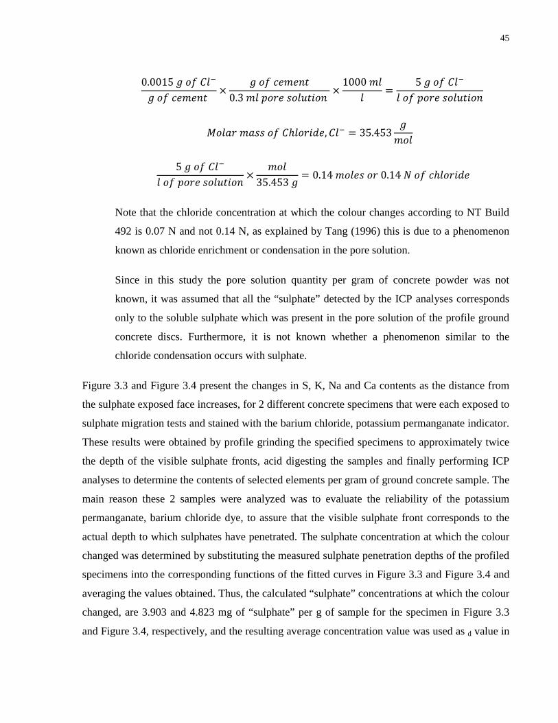
45
0.0015 𝑔 𝑜𝑓 𝐶𝑙−
𝑔 𝑜𝑓 𝑐𝑒𝑚𝑒𝑛𝑡 ×
𝑔 𝑜𝑓 𝑐𝑒𝑚𝑒𝑛𝑡0.3 𝑚𝑙 𝑝𝑜𝑟𝑒 𝑠𝑜𝑙𝑢𝑡𝑖𝑜𝑛
×1000 𝑚𝑙
𝑙=
5 𝑔 𝑜𝑓 𝐶𝑙−
𝑙 𝑜𝑓 𝑝𝑜𝑟𝑒 𝑠𝑜𝑙𝑢𝑡𝑖𝑜𝑛
𝑀𝑜𝑙𝑎𝑟 𝑚𝑎𝑠𝑠 𝑜𝑓 𝐶ℎ𝑙𝑜𝑟𝑖𝑑𝑒,𝐶𝑙− = 35.453𝑔𝑚𝑜𝑙
5 𝑔 𝑜𝑓 𝐶𝑙−
𝑙 𝑜𝑓 𝑝𝑜𝑟𝑒 𝑠𝑜𝑙𝑢𝑡𝑖𝑜𝑛×
𝑚𝑜𝑙35.453 𝑔
= 0.14 𝑚𝑜𝑙𝑒𝑠 𝑜𝑟 0.14 𝑁 𝑜𝑓 𝑐ℎ𝑙𝑜𝑟𝑖𝑑𝑒
Note that the chloride concentration at which the colour changes according to NT Build
492 is 0.07 N and not 0.14 N, as explained by Tang (1996) this is due to a phenomenon
known as chloride enrichment or condensation in the pore solution.
Since in this study the pore solution quantity per gram of concrete powder was not
known, it was assumed that all the “sulphate” detected by the ICP analyses corresponds
only to the soluble sulphate which was present in the pore solution of the profile ground
concrete discs. Furthermore, it is not known whether a phenomenon similar to the
chloride condensation occurs with sulphate.
Figure 3.3 and Figure 3.4 present the changes in S, K, Na and Ca contents as the distance from
the sulphate exposed face increases, for 2 different concrete specimens that were each exposed to
sulphate migration tests and stained with the barium chloride, potassium permanganate indicator.
These results were obtained by profile grinding the specified specimens to approximately twice
the depth of the visible sulphate fronts, acid digesting the samples and finally performing ICP
analyses to determine the contents of selected elements per gram of ground concrete sample. The
main reason these 2 samples were analyzed was to evaluate the reliability of the potassium
permanganate, barium chloride dye, to assure that the visible sulphate front corresponds to the
actual depth to which sulphates have penetrated. The sulphate concentration at which the colour
changed was determined by substituting the measured sulphate penetration depths of the profiled
specimens into the corresponding functions of the fitted curves in Figure 3.3 and Figure 3.4 and
averaging the values obtained. Thus, the calculated “sulphate” concentrations at which the colour
changed, are 3.903 and 4.823 mg of “sulphate” per g of sample for the specimen in Figure 3.3
and Figure 3.4, respectively, and the resulting average concentration value was used as d value in

46
the migration coefficient equation is 4.363 mg of “sulphate”/g of concrete powder or 4.54x10⁻⁵
moles:
0.004363 𝑔 𝑜𝑓 𝑆𝑂42−
96.0626 𝑔𝑚𝑜𝑙
= 4.54 × 10⁻⁵ 𝑚𝑜𝑙𝑒𝑠 𝑜𝑓 𝑠𝑢𝑙𝑝ℎ𝑎𝑡𝑒.
Figure 3.3 Change in total S, Na, K and Ca contents of concrete with change in distance
from sulphate exposed face. Sample was ~6.5 months old, tested in modified NT Build 492
for 4 days in 10% Na2SO4 solution. Sample properties: 0.5 w/cm, GU cement, 35 % slag,
average visible sulphate front was 3.25 mm deep.
Total Sulphur
Total Sodium
Total Potassium
Total Calcium
y = 0.002x4 - 0.0572x3 + 0.6369x2 - 3.5163x + 10.344R² = 0.9918
130
140
150
160
170
180
190
200
210
220
230
0
1
2
3
4
5
6
7
8
9
10
0 1 2 3 4 5 6 7 8 9 10 11
Ca co
ncen
trat
ion
mg
of e
lem
ent/
g of
sam
ple
S, N
a &
K C
once
ntra
tions
mg
of e
lem
ent/
g of
sam
ple
Distance from sulphate exposed face (mm)
Outlier

47
Figure 3.4 Change in total S, Na, K and Ca contents of concrete with change in distance
from sulphate exposed face. Sample was 56 days old, tested in modified NT Build 492 for 1
day in 10% Na2SO4 solution. Sample properties: 0.4 w/cm, HS cement, average visible
sulphate front was 1.35 mm deep.
Considering that,
1. These are total sulphur contents rather than soluble sulphate contents.
2. The 2 specimens tested had different water to cement ratios, cement types and slag
replacement percentages.
3. Results of the sample presented in Figure 3.3 are the least accurate since slag is present.
It is reasonable to state that these two concentration values are close enough to verify the
validity of the potassium permanganate, barium chloride dye. Of course, additional tests
which determine the actual soluble sulphate content, and determine more accurately the
sulphate concentration at which the colour changes, would help further validate this
statement.
Total Sulphur
Total Sodium
Total Potassium
Total Calcium
y = 0.0188x4 - 0.3629x3 + 2.6271x2 - 8.5501x + 12.407R² = 0.9998
130
140
150
160
170
180
190
200
210
220
230
0
1
2
3
4
5
6
7
8
9
10
0 1 2 3 4 5 6 7
Ca C
once
ntra
tion
mg
of e
lem
ent/
g of
sam
ple
S, N
a &
K C
once
ntra
tions
mg
of e
lem
ent/
g of
sam
ple
Distance from sulphate exposed face (mm)

48
3.3.3 Modified NT Build 492 Test Duration: Test Set-up Enabling the Recording of the Current throughout the Test
The test set-up for NT Build 492, unlike ASTM C 1202, does not have the option of
automatically recording the current throughout the test duration. Since several NT Build 492
tests were to run under modified test duration of 4 and 9 days, it was of interest to monitor the
change in current throughout the test and calculated the total charge passing at the end of the
tests. To accomplish this, two ICP DAS data acquisition devices were connected as shown in
Figure 3.5.
As may be observed from Figure 3.5, an ICP DAS 8 channel (although Figure 3.5 only shows 2)
universal analog input module (part number i-7019R) was used to measure the current. This
module (which was directly connected to a DC power supply) was then connected to an ICP
DAS USB converter (part number i-7561) which transferred the data to DASYLab®, data
acquisition software.
The input module’s current measurement range is ±20 mA, however, the currents going through
the concrete specimens were higher. For this reason, it was necessary to measure the current
indirectly by measuring the voltage drop across each specimen. However, once again the range
of the module was below the requirements, as the maximum voltage input was 10 volts, and the
test voltages ranged from 30 to 50 volts. Therefore, to overcome this limitation, a 100 ohm
exterior resistor was connected in series to each of the circuit sub-sections as shown in Figure
3.5, such that the voltage drop across the resistor could be measured by the input module.

49
Figure 3.5 Circuit diagram of the NT Build 492 with modified test duration set-up used in
this study to record the change in current throughout the modified test duration. Note that
all the blocks connected to the ICP DAS devices are terminal names specific to each device.
It is important to note that the addition of the 100 ohm resistor in series signifies that a portion of
the applied voltage will be used by the resistor. For instance, assuming the resistance of the
concrete sample at the beginning of the test is 1000 ohms and the applied test voltage is 35 volts,
the current in going through the concrete sample and the 100 ohms resistor can be determined as
follows,

50
𝑅𝑐𝑜𝑛𝑐𝑟𝑒𝑡𝑒 𝑠𝑎𝑚𝑝𝑙𝑒 = 1000 𝑜ℎ𝑚𝑠 ; 𝑅𝑟𝑒𝑠𝑖𝑠𝑡𝑜𝑟 = 100 𝑜ℎ𝑚𝑠
∴ 𝑅𝑇𝑜𝑡𝑎𝑙, = 1100 𝑜ℎ𝑚𝑠
𝑇𝑒𝑠𝑡 𝑉𝑜𝑙𝑡𝑎𝑔𝑒 = 35 𝑣𝑜𝑙𝑡𝑠 ∴ 𝐼 = 𝑇𝑒𝑠𝑡 𝑣𝑜𝑙𝑡𝑎𝑔𝑒
𝑅𝑇𝑜𝑡𝑎𝑙= 31.82 𝑚𝐴
Using this calculated current, the voltage drop across the 100 ohm resistor is calculated to be
3.182 volts, meaning that the actual voltage drop across the concrete sample is 31.818 volts, 9 %
less than the original test voltage of 35 volts. This difference between the actual voltage applied
to the sample and the original test voltage applied to the whole system, decreases as the
resistivity of the concrete specimen increases. Table 3.4 and
Table 3.5 present the test voltage applied to the system, the initial current measured in the
system, the calculated voltage drops across the resistor and the specimen, and the percent
difference between the test voltage and the actual voltage applied to the specimen.
Since the currents in these tests were recorded at 5 minutes intervals, the change in applied
voltage was taken into consideration when calculating the change in resistivity throughout the
test duration. To calculate the migration coefficients, the average applied voltage was used. The
total charge passing throughout the test duration was calculated by calculating the area under the
current vs. time plot, using the trapezoidal rule.
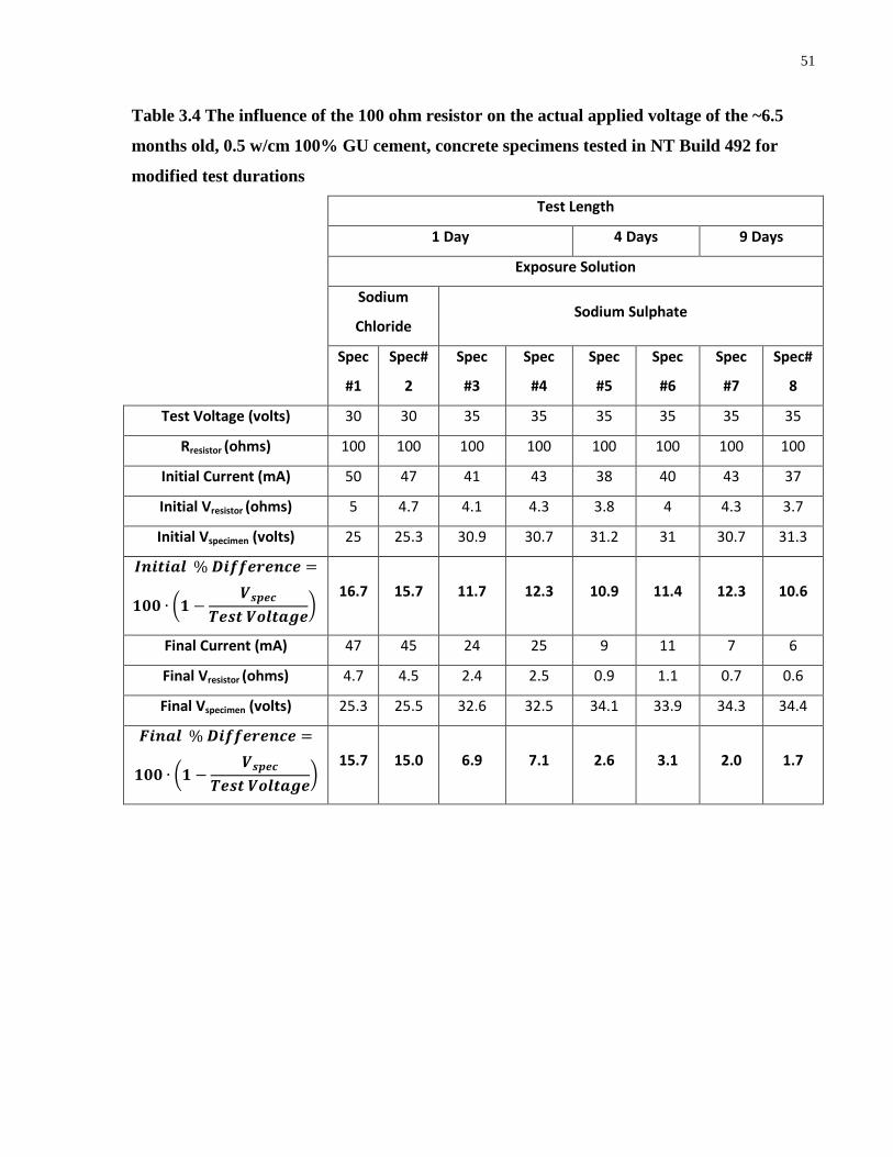
51
Table 3.4 The influence of the 100 ohm resistor on the actual applied voltage of the ~6.5
months old, 0.5 w/cm 100% GU cement, concrete specimens tested in NT Build 492 for
modified test durations
Test Length
1 Day 4 Days 9 Days
Exposure Solution
Sodium
Chloride Sodium Sulphate
Spec
#1
Spec#
2
Spec
#3
Spec
#4
Spec
#5
Spec
#6
Spec
#7
Spec#
8
Test Voltage (volts) 30 30 35 35 35 35 35 35
Rresistor (ohms) 100 100 100 100 100 100 100 100
Initial Current (mA) 50 47 41 43 38 40 43 37
Initial Vresistor (ohms) 5 4.7 4.1 4.3 3.8 4 4.3 3.7
Initial Vspecimen (volts) 25 25.3 30.9 30.7 31.2 31 30.7 31.3
𝑰𝒏𝒊𝒕𝒊𝒂𝒍 % 𝑫𝒊𝒇𝒇𝒆𝒓𝒆𝒏𝒄𝒆 =
𝟏𝟎𝟎 ∙ �𝟏 −𝑽𝒔𝒑𝒆𝒄
𝑻𝒆𝒔𝒕 𝑽𝒐𝒍𝒕𝒂𝒈𝒆�
16.7 15.7 11.7 12.3 10.9 11.4 12.3 10.6
Final Current (mA) 47 45 24 25 9 11 7 6
Final Vresistor (ohms) 4.7 4.5 2.4 2.5 0.9 1.1 0.7 0.6
Final Vspecimen (volts) 25.3 25.5 32.6 32.5 34.1 33.9 34.3 34.4
𝑭𝒊𝒏𝒂𝒍 % 𝑫𝒊𝒇𝒇𝒆𝒓𝒆𝒏𝒄𝒆 =
𝟏𝟎𝟎 ∙ �𝟏 −𝑽𝒔𝒑𝒆𝒄
𝑻𝒆𝒔𝒕 𝑽𝒐𝒍𝒕𝒂𝒈𝒆�
15.7 15.0 6.9 7.1 2.6 3.1 2.0 1.7

52
Table 3.5 The influence of the 100 ohm resistor on the applied voltage of the ~6.5 months
old, 0.5 w/cm, GU cement with 35 % slag replacement, concrete specimens tested in NT
Build 492 for modified test durations
Test Length
1 Day 4 Days 9 Days
Exposure solution
Sodium
Chloride Sodium Sulphate
Spec
#1
Spec#
2
Spec
#3
Spec
#4
Spec
#5
Spec
#6
Spec
#7
Spec#
8
Test Voltage (volts) 35 35 50 50 50 50 50 50
Rresistor (ohms) 100 100 100 100 100 100 100 100
Initial Current (mA) 47 36.5 29 27 31 27 28 30
Initial Vresistor (ohms) 4.7 3.65 2.9 2.7 3.1 2.7 2.8 3
Initial Vspecimen (volts) 30.3 31.35 47.1 47.3 46.9 47.3 47.2 47
𝑰𝒏𝒊𝒕𝒊𝒂𝒍 % 𝑫𝒊𝒇𝒇𝒆𝒓𝒆𝒏𝒄𝒆 =
𝟏𝟎𝟎 ∙ �𝟏 −𝑽𝒔𝒑𝒆𝒄
𝑻𝒆𝒔𝒕 𝑽𝒐𝒍𝒕𝒂𝒈𝒆�
13.4 10.4 5.8 5.4 6.2 5.4 5.6 6.0
Final Current (mA) 41 46 16 16 11 10 9 9
Final Vresistor (ohms) 4.1 4.6 1.6 1.6 1.1 1 0.9 0.9
Final Vspecimen (volts) 30.9 30.4 48.4 48.4 48.9 49 49.1 49.1
𝑭𝒊𝒏𝒂𝒍 % 𝑫𝒊𝒇𝒇𝒆𝒓𝒆𝒏𝒄𝒆 =
𝟏𝟎𝟎 ∙ �𝟏 −𝑽𝒔𝒑𝒆𝒄
𝑻𝒆𝒔𝒕 𝑽𝒐𝒍𝒕𝒂𝒈𝒆�
11.7 13.1 3.2 3.2 2.2 2.0 1.8 1.8
3.3.4 Bulk Electrical Resistivity Tests
Prior to starting the electrical migration tests, the resistivity of each concrete specimen was
measured first using the Monfore and then Merlin instruments. The resistivities of each specimen
were measured again once the migration tests were completed to measure the Monfore and
Merlin resistivities of each specimen after the exposure to the aggressive ions. Both methods are
non-destructive and are not known to influence the composition or composition of the concrete.

53
3.3.4.1 DC (Monfore) Bulk Electrical Resistivity
This test method, used by El-Dieb et al. in their unpublished paper, at the University of Toronto,
is described by the authors to be similar to the test method used by Monfore (1968). Therefore,
although this test method is not exactly the same as the test method used by Monfore (1968), this
test method will be referred to as the Monfore bulk electrical resistivity test.
The test used by El-Dieb et al. (Unpublished) involved subjecting concrete specimens to DC
potentials which alternated between 3 and 5 volts every 5 seconds. The specimens used were
water saturated (as per ASTM C 1202) concrete discs of the same size as the specimens used in
this study. Prior to initiating the test, the curved sides of specimens were coated with epoxy and
the cut surfaces of the discs were covered with water soluble, salt free conductive gel. A
schematic diagram of the test set-up, extracted from the unpublished paper by El-Dieb et al. is
shown in Figure 3.6. Test duration was 15 minutes.
In this study, unlike the procedure by El-Dieb et al., the curved sides of the specimen were
wrapped with vinyl electrical tape and the test duration was 5 minutes. These changes were made
to ensure that all 8 specimens were tested at the same work day, since a 3 hour water saturation
took place prior to measuring the Merlin bulk electrical resistivity following the Monfore
measurements.
The concrete discs were placed between the stainless steel electrodes such that the face to be
exposed to the aggressive ions was in contact with the negative electrode. Once the test was
finished, the electrical tape was removed and the conductive gel was washed away using tap
water.
The resistivity was calculated as follows (El-Dieb et al., Unpublished):
𝑅𝑒𝑠𝑖𝑠𝑡𝑖𝑣𝑖𝑡𝑦 (𝑜ℎ𝑚 ∙ 𝑐𝑚) =(𝑉5 − 𝑉3) × 𝐴(𝐼5 − 𝐼3) × 𝐿
Eq. 3.4
Where V5 and V3 are the average applied voltage for 5 and 3 volts respectively and I5 and I3 are
the average currents for 5 volts and 3 volts respectively, measured in amperes. A is the cross-
sectional area of the specimens measured in cm2 and L is the thickness of the specimen in cm.

54
Figure 3.6 Schematic diagram of the DC (Monfore) bulk electrical resistivity test set-up
used in this study (El-Dieb et al., Unpublished)
3.3.4.2 Merlin Bulk Electrical Resistivity
In this test method (performed following the Monfore resistivity measurements), current from an
alternating current source went through the saturated specimens. A voltmeter, connected to the
instrument, measured the voltage drop across the specimen while an ammeter measured the
current. The cut faces of the water saturated specimens were kept moist using moist sponges.
Prior to initiating the test, the thin sponges attached to the Merlin instrument were wetted using
distilled water spray bottle, and the instrument was calibrated using the verification cylinder
available. The Merlin instrument measured the resistivity of the specimens within 2 seconds. A
schematic of the measurement method is presented in Figure 3.7 and the test apparatus is
presented Figure 3.8.

55
Figure 3.7 Schematic diagram of the measurement method used in the Merlin instrument
(Germann Instruments, 2010)
Figure 3.8 Merlin bulk electrical resistivity apparatus
(http://www.germann.org/?strArticle=news)
3.3.5 Compressive Strength Test
Compressive strength tests were performed at 7 and 28 days. Due to limited number of cylinders,
one cylinder was tested per age.

56
Chapter 4 Results: Observations and Discussion
4
4.1 Overview As described in Chapter 3, nine concrete mix designs were tested to compare both the original
chloride migration test to the modified sulphate migration test. Relevant details of these mixtures
are presented in Table 4.1. Essentially, the goal is to determine whether performing either the
Nord Test NT 492 rapid migration test or ASTM C 1202 rapid permeability test with chloride or
sulphate produces results which are to an extent unique to the exposure solution. That is, are
these tests only generally related to ion penetration resistance, or is it also possible to
differentiate between cement types and thus identify sulphate resistant in addition to chloride
resistant concretes?
The effectiveness of the developed rapid sulphate test was determined by:
1. Comparing the standard chloride migration test results to the sulphate migration test
results.
2. Comparing the sulphate migration test results obtained for the different concrete
mixtures.
3. Evaluating the ability of the barium chloride, potassium permanganate dye to clearly
identify the sulphate front, and the ability of the sulphate ions to penetrate deeply enough
within the accelerated test period. Enough variation must be present such that the
differences may be attributed to mix designs and cement types rather than acceptable
differences due to experimental variability
In addition to evaluating the sulphate migration test, the relationships between electrical
resistivity measurements obtained from both migration tests, NT Build 492 and ASTM C 1202,
and the Monfore and Merlin Bulk Electrical Resistivity tests were determined. As well, the
relationship between these resistivity values and the total charge values obtained from ASTM C
1202 and the diffusion coefficient obtained from NT Build 492 were examined.

57
Table 4.1 Summary of concrete mixtures tested and their properties
Mix
No. Mix ID
Mix Properties
w/cm Cement
Type
Slag
Replacement
(%)
Cement C3A
Content (%)
Cement C2S
Content (%)
1 0.5/GU/35S 0.5
Holcim GU
35
10.7 28.0 2 0.5/GU 0.5 -
3 0.45/GU/50S 0.45 50
4 0.4/GU/50S 0.4 50
5 0.5/InterCem 0.5
Lehigh
InterCem
GUb-30F
-
6 0.45/HS 0.45 Lehigh HS
- 2.5 17.4
7 0.4/HS 0.4 -
8 0.5/MS 0.5 Lehigh GU
(or MS in
this paper)
- 5.5 13.9
9 0.4/MS/50S 0.4 50
Based on Section 2.10 in the Literature Review chapter, which discusses the variables affecting
test results, the following results were expected:
1. Regardless of the exposure solution, older concrete specimens of lower water to
cement/binder ratios and with higher slag and fly ash replacements were expected to
have:
a. Lower amounts of total charge passing during the rapid penetration tests.
b. Lower migration coefficients
c. Smaller depths of penetration

58
d. Higher initial bulk electrical resistivity values.
2. Regardless of the exposure solution and for the same mix designs, concrete specimens
containing type GU cement, with the highest C3A and C2S contents were expected to
have:
a. The lowest amounts of total charge passing during the rapid penetration tests.
b. The lowest migration coefficients.
c. The Smallest depths of penetration.
d. The highest initial bulk electrical resistivity values.
3. In comparison to concrete specimens exposed to sodium chloride, under the original
standard tests, specimens exposed to sodium sulphate were expected to have:
a. Lower amounts of total charge passing during the rapid penetration tests.
b. Lower penetration depths.
c. Lower migration coefficients.
4.2 Plastic Properties and Compressive Strengths The measured plastic properties of the mixtures tested are presented in Table 4.2. A slump range
of 60 to 120 mm was targeted.
A total of 10 cylinders were cast per mix, 8 of which were used for the migration tests. The
mixer used had a capacity of 18 litres. The remaining two cylinders were tested for their
compressive strengths, 1 cylinder was tested at 7 days and the other at 28 days. The results of
these tests are presented in Table 4.2. Since only one cylinder was tested per test age, a
comparison of the compressive strengths obtained for the different mixtures will not provide
adequate representation of the quality of the entire batch. Therefore, these compressive strength
results were used only as an indication, assuring that each mix had an acceptable strength prior to
performing the migration tests on the concrete specimens. However, it should be noted that the
compressive strengths of all but 0.4/HS and 0.5/MS mixtures increase with age, although, the 28
days strengths of these two mixtures seem more reasonable than those obtained at 7 days, which
were higher than expected. The migration tests were performed on 35 and 56 days old
specimens. Due to the limited number of cylinders, only two cylinders per mix were available for
compressive strength testing. It was decided to measure the 7 and 28 days rather than the 35 and

59
56 days compressive strengths in order to obtain an indication of the quality of the concrete
mixtures earlier.
Table 4.2 Compressive strength and plastic properties of fresh concrete
Mix No. Mix ID Mix
Properties
Compressive Strength
(MPa) Slump
(mm)
Plastic
Density
(kg/m3) Age
7 Days 28 Days
1
0.5/GU/35S w/cm=0.5;
GU cement;
35% slag
24.7 31.2 100 2430
T5* - 80 -
2 0.5/GU w/cm=0.5;
GU cement
27.9 33.8 75 2419
T3* - - 75 -
3 0.45/GU/50S
w/cm=0.45;
GU cement;
50% slag
29.0 40.1 60 2411
4 0.4/GU/50S
w/cm=0.4;
GU cement;
50% slag
33.7** 39.2 110 2433
5 0.5/InterCem
w/cm=0.5;
InterCem
(Fly ash
blended)
23.3 37.6 115 2424
6 0.45/HS w/cm=0.45;
HS cement 25.7 26.4 120 2401
7 0.4/HS w/cm=0.4;
HS cement 37.7 33.8 90 2449
8 0.5/MS w/cm=0.5;
MS cement 32.9 30.4 100 2431
9 0.4/MS/50S
w/cm=0.4;
MS cement;
50% slag
42.8 42.8 100 2449
*T5 and T3 are additional batches of Mix 1 and 2, respectively, which were used in the NT Build
492 test with modified test durations.
** Tested at 8 days

60
Please note that from this point on, the nine mixtures investigated will be referred to by their mix
ID. Also, unless otherwise noted, the term “average results” in this paper, refers to the average of
the 2 specimens which were tested for each testing condition.
4.3 Rapid Permeability Test Results 4.3.1 Total 6 hours Charge, Q6hrs
The total 6 hours charge values, Q6hrs, passing through the chloride and sulphate specimens are
presented in Table 4.3 and Table 4.4, respectively. The following observations are common to
both chloride and sulphate results. As expected, Q6hrs values of specimens containing slag and fly
ash are notably lower than those of specimens with 100% cement, and all values decrease with
age. A comparison of the overall average charge value obtained at 35 days to the value obtained
at 56 (Table 4.3 and Table 4.4) shows that the 56 day results are 12% and 14% lower than the 35
day values for chloride and sulphate tests, respectively.
Regardless of the exposure solution, the specimens containing 100% HS or MS cements showed
the highest amount of charge passed and the steepest decrease in Q6hrs was seen with the
0.5/InterCem mix which contained 30% fly ash. Significant decrease in Q6hrs with age was also
seen with the 0.4/HS mix.
Table 4.3 Rapid chloride permeability test specimens, 6 hours charge values, 𝑸𝟔𝒉𝒓𝒔,𝑵𝒂𝒄𝒍
(coulombs).
Mix ID
Rapid Chloride Permeability Test 𝑸𝟔𝒉𝒓𝒔,𝑵𝒂𝒄𝒍 (coulombs)
Age 35 Days 56 Days
Specimen 1 Specimen 2 Average Specimen 1 Specimen 2 Average 0.5/GU/35S 987 1001 994 867 887 877
0.5/GU 2506 2407 2456 2260 2149 2205 0.45/GU/50S 709 742 726 589 572 581 0.4/GU/50S 804 765 784 653 611 632
0.5/InterCem 1000 950 975 592 622 607 0.45/HS 3456 3263 3360 2759 3299 3029 0.4/HS 3139 3134 3137 2583 2776 2680 0.5/MS 2992 3364 3178 3074 2950 3012
0.4/MS/50S 811 805 808 728 822 775
Average 1824 Average 1600

61
Table 4.4 Rapid sulphate permeability test specimens, 6 hours charge values 𝑸𝟔𝒉𝒓𝒔,𝑵𝒂𝟐𝑺𝑶𝟒,
(coulombs).
Mix ID
Rapid Sulphate Permeability Test 𝑸𝟔𝒉𝒓𝒔,𝑵𝒂𝟐𝑺𝑶𝟒 (coulombs)
Age 35 Days 56 Days
Specimen 1 Specimen 2 Average Specimen 1 Specimen 2 Average 0.5/GU/35S 947 855 901 691 801 746
0.5/GU 1941 1998 1970 1528 1640 1584 0.45/GU/50S 584 721 653 454 560 507 0.4/GU/50S 557 679 618 581 614 597
0.5/InterCem 871 898 884 541 513 527 0.45/HS 2361 2158 2260 1945 2456 2200 0.4/HS 2295 2558 2426 1919 1894 1906 0.5/MS 2222 2120 2171 2141 2058 2099
0.4/MS/50S 617 704 660 562 677 620
Average 1394 Average 1198
It may be observed that in addition to the decrease in charge values with age, the average charge
values obtained from the rapid sulphate permeability tests are lower than the values obtained
from the rapid chloride tests. The percent differences between 𝑄6ℎ𝑟𝑠,𝑁𝑎𝑐𝑙 and 𝑄6ℎ𝑟𝑠,𝑁𝑎2𝑆𝑂4 of
each mix are presented in Table 4.5 where it may be observed that the overall average percent
difference between the rapid chloride and sulphate permeability tests is approximately the same
at 35 and 56 days.
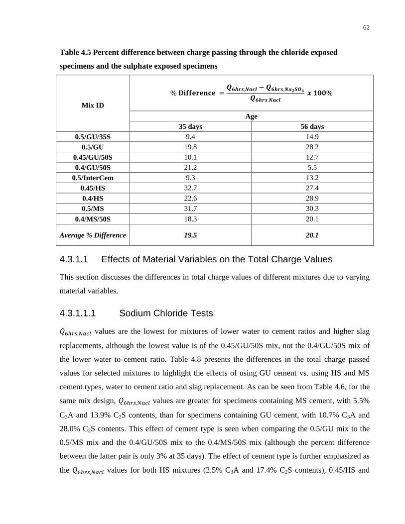
62
Table 4.5 Percent difference between charge passing through the chloride exposed
specimens and the sulphate exposed specimens
Mix ID
% 𝐃𝐢𝐟𝐟𝐞𝐫𝐞𝐧𝐜𝐞 =𝑸𝟔𝒉𝒓𝒔,𝑵𝒂𝒄𝒍 − 𝑸𝟔𝒉𝒓𝒔,𝑵𝒂𝟐𝑺𝑶𝟒
𝑸𝟔𝒉𝒓𝒔,𝑵𝒂𝒄𝒍 𝒙 𝟏𝟎𝟎%
Age
35 days 56 days 0.5/GU/35S 9.4 14.9
0.5/GU 19.8 28.2 0.45/GU/50S 10.1 12.7 0.4/GU/50S 21.2 5.5
0.5/InterCem 9.3 13.2 0.45/HS 32.7 27.4 0.4/HS 22.6 28.9 0.5/MS 31.7 30.3
0.4/MS/50S 18.3 20.1
Average % Difference 19.5 20.1
4.3.1.1 Effects of Material Variables on the Total Charge Values
This section discusses the differences in total charge values of different mixtures due to varying
material variables.
4.3.1.1.1 Sodium Chloride Tests
𝑄6ℎ𝑟𝑠,𝑁𝑎𝑐𝑙 values are the lowest for mixtures of lower water to cement ratios and higher slag
replacements, although the lowest value is of the 0.45/GU/50S mix, not the 0.4/GU/50S mix of
the lower water to cement ratio. Table 4.8 presents the differences in the total charge passed
values for selected mixtures to highlight the effects of using GU cement vs. using HS and MS
cement types, water to cement ratio and slag replacement. As can be seen from Table 4.6, for the
same mix design, 𝑄6ℎ𝑟𝑠,𝑁𝑎𝑐𝑙 values are greater for specimens containing MS cement, with 5.5%
C3A and 13.9% C2S contents, than for specimens containing GU cement, with 10.7% C3A and
28.0% C2S contents. This effect of cement type is seen when comparing the 0.5/GU mix to the
0.5/MS mix and the 0.4/GU/50S mix to the 0.4/MS/50S mix (although the percent difference
between the latter pair is only 3% at 35 days). The effect of cement type is further emphasized as
the 𝑄6ℎ𝑟𝑠,𝑁𝑎𝑐𝑙 values for both HS mixtures (2.5% C3A and 17.4% C2S contents), 0.45/HS and

63
0.4/HS, are higher than that of the GU mix, 0.5/GU, even though the latter has a higher water to
cement ratio. The 0.5/GU also had higher compressive strength at 28 days than both 0.45/HS and
0.4/HS mixtures. That is, increases of 8.2% in the C3A and 10.6% in the C2S contents had greater
impact on the total charge passing through a concrete disc than reducing the w/cm from 0.5 to
0.4. Although is it not known whether the this influence is due to a higher degree of hydration
(due to C2S content), due to higher binding capacity (due to high C3A content), or a combination
of both. The effect of reducing the w/cm from 0.45 to 0.4 on the total charge passing is also seen
in Table 4.6. For both the GU and HS mixtures, the reduction of the water to cement ratio from
0.45 to 0.4 resulted in relatively small differences. The percent difference between the 0.5/GU
and the 0.5/GU/35S mixtures on the other hand, are very high. The 35% replacement of GU
cement by slag for a 0.5 w/cm mix, reduced the total charge value by 60% at both 35 and 56
days.
Table 4.6 Differences in total charge passed during the rapid chloride permeability tests for
selected mixtures
𝑴𝒊𝒙 #𝟏
−𝑴𝒊𝒙 #𝟐
𝑸�𝟔𝒉𝒓𝒔,𝑵𝒂𝒄𝒍 𝒐𝒇 𝑴𝒊𝒙 #𝟏− 𝑸�𝟔𝒉𝒓𝒔,𝑵𝒂𝒄𝒍 𝒐𝒇 𝑴𝒊𝒙 #𝟐
(coulombs)
% 𝑫𝒊𝒇𝒇𝒆𝒓𝒆𝒏𝒄𝒆
= �𝑸�𝟔𝒉𝒓𝒔,𝑵𝒂𝒄𝒍 𝒐𝒇 𝑴𝒊𝒙 #𝟏 − 𝑸�𝟔𝒉𝒓𝒔,𝑵𝒂𝒄𝒍 𝒐𝒇 𝑴𝒊𝒙 #𝟐
𝑸�𝟔𝒉𝒓𝒔,𝑵𝒂𝒄𝒍 𝒐𝒇 𝑴𝒊𝒙 #𝟏�
× 𝟏𝟎𝟎%
Age Age 35 Days 56 Days 35 Days 56 Days
Effect of GU vs. MS and HS cements types 0.4/MS/50S – 0.4 /GU/50S 24 143 3% 19%
0.5/MS – 0.5/GU 722 807 23% 27%
0.4/HS – 0.5/GU 680 475 22% 18%
Effect of Water to Cement Ratio 0.45/GU/50S –
0.4/GU/50S -59 -51 -8% -9%
0.45/HS – 0.4/HS 223 349 7% 12%
Effect of Slag Replacement 0.5/GU –
0.5/GU/35S 1462 1328 60% 60%

64
4.3.1.1.2 Sodium Sulphate Tests
Table 4.7 presents the differences in the total charge passed for selected mixtures to highlight the
effects of using GU cement vs. using HS and MS cement types, water to cement ratio and slag
replacement. Similar to the chloride exposed specimens, for the same mix design, 𝑄6ℎ𝑟𝑠,𝑁𝑎2𝑆𝑂4
values are greater for specimens containing MS cement, than for specimens containing GU
cement. However, as can be seen from Table 4.7, for the specimens exposed to sulphate, the
percent differences in total charge between mixtures containing MS cement and those containing
GU cement are not as high as the percent differences for the specimens exposed to chlorides
(except when comparing the 0.5/MS mix to the 0.5/GU mix at 56 days). That is, for the same
mix design, the rapid sulphate permeability values do not differentiate between concretes
mixtures containing MS or GU cements as well as the rapid chloride permeability test.
However, similar to the rapid chloride test, the sulphate test was able to distinguish between the
0.4/HS mix and the 0.5/GU mix, and as with the chloride tests, the 0.5/GU mix had lower charge
value than the 0.4/HS mix with the lower water to cement ratio.
As may be seen from Table 4.6 and Table 4.7, the percent differences in charge values when
reducing the water to cement ratio of concrete from 0.45 to 0.4, were similar and are relatively
low, for both the rapid chloride and sulphate permeability tests at 35 days. The percent
differences are greater for the sulphate test at 56 days.
As with the rapid chloride test, the rapid sulphate test was able to clearly distinguish between the
GU mix with slag, 0.5/GU/35S and the mix without the slag replacement, 0.5/GU. As presented
in Table 4.7, in the case of the rapid sulphate permeability test, the 35% replacement of cement
with slag reduced the total charge values by an average of 53.5%.

65
Table 4.7 Differences in total charge passed during the rapid sulphate permeability tests
for selected mixtures
𝑴𝒊𝒙 #𝟏
−𝑴𝒊𝒙 #𝟐
𝑸�𝟔𝒉𝒓𝒔,𝑵𝒂𝟐𝑺𝑶𝟒𝒐𝒇 𝑴𝒊𝒙 #𝟏− 𝑸�𝟔𝒉𝒓𝒔,𝑵𝒂𝟐𝑺𝑶𝟒𝒐𝒇 𝑴𝒊𝒙 #𝟐
(coulombs)
% 𝑫𝒊𝒇𝒇𝒆𝒓𝒆𝒏𝒄𝒆
= �𝑸�𝟔𝒉𝒓𝒔,𝑵𝒂𝟐𝑺𝑶𝟒𝒐𝒇 𝑴𝒊𝒙 #𝟏 − 𝑸�𝟔𝒉𝒓𝒔,𝑵𝒂𝟐𝑺𝑶𝟒𝒐𝒇 𝑴𝒊𝒙 #𝟐
𝑸�𝟔𝒉𝒓𝒔,𝑵𝒂𝟐𝑺𝑶𝟒 𝒐𝒇 𝑴𝒊𝒙 #𝟏�
× 𝟏𝟎𝟎%
Age Age 35 Days 56 Days 35 Days 56 Days
Effect of GU vs. MS and HS cements types 0.4/MS/50S – 0.4 /GU/50S 42 22 6% 4%
0.5/MS – 0.5/GU 201 515 9% 25%
0.4/HS – 0.5/GU 456 323 19% 17%
Effect of Water to Cement Ratio 0.45/GU/50S –
0.4/GU/50S 35 -90 5% -18%
0.45/HS – 0.4/HS -166 294 -7% 13%
Effect of Slag Replacement 0.5/GU –
0.5/GU/35S 1069 838 54% 53%
4.3.2 Qualitatively Evaluating Sulphate Ion Penetrability into Concrete
The original ASTM C 1202 standard test includes a table which contains ranges of charge passed
values along with corresponding qualitative evaluation of the chloride ion penetrability (see
Section 2.5.2.1). In order to develop a similar table which is suited for sulphate ion penetrability,
the total charge values of the specimens exposed to sulphates were plotted against the total
charge values of the specimens exposed to chlorides. Since for each concrete cylinder, one disk
was exposed to chlorides and the other to sulphates, the total charge value of the chloride-
exposed specimen was plotted against the total charge value of the sulphate-exposed specimen
cut from the same cylinder. This plot is presented in Figure 4.1 with a linear line of best fit. To
determine the ranges of the sulphate penetrability table, the original values of the table in ASTM
C 1202 were inserted in the function of the line of best fit in Figure 4.1 and the values were
rounded down to the next 100 coulombs. The lowest charge value in the ASTM C 1202 original
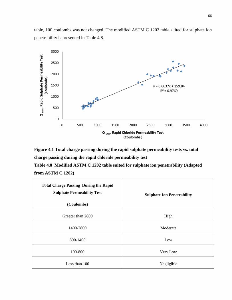
66
table, 100 coulombs was not changed. The modified ASTM C 1202 table suited for sulphate ion
penetrability is presented in Table 4.8.
Figure 4.1 Total charge passing during the rapid sulphate permeability tests vs. total
charge passing during the rapid chloride permeability test
Table 4.8 Modified ASTM C 1202 table suited for sulphate ion penetrability (Adapted
from ASTM C 1202)
Total Charge Passing During the Rapid
Sulphate Permeability Test
(Coulombs)
Sulphate Ion Penetrability
Greater than 2800 High
1400-2800 Moderate
800-1400 Low
100-800 Very Low
Less than 100 Negligible
y = 0.6637x + 159.84R² = 0.9769
0
500
1000
1500
2000
2500
3000
0 500 1000 1500 2000 2500 3000 3500 4000
Q 6h
rs, R
apid
Sul
phat
e Pe
rmea
bilit
y Te
st(C
oulo
mbs
)
Q 6hrs, Rapid Chloride Permeability Test(Coulombs )

67
4.3.3 Resistivity
During the rapid permeability tests the current of each specimen was recorded at 1 and 5
minutes. Using these currents, I, recorded in mA, the test voltage, V, and Ohm’s Law (𝑅 = 𝑉𝐼),
instantaneous 1 and 5 minute electrical resistance values, R values, were determined in ohms.
Then, using these R values, the measured cross-sectional area and length of every specimen and
mathematical relationship between the electrical resistance and resistivity, 𝜌 = 𝑅 𝐴𝑙, the electrical
resistivity, 𝜌, of each specimen was determined in ohm∙m. The calculated instantaneous 1 and 5
minute and average 6 hour resistivity values are summarized in Table 4.9 and Table 4.10 for
chloride and sulphate, respectively. Since the average 6 hour resistivity values are derived from
the total charge values, as already discussed, the trends and observations are the same, except
inversed.
Table 4.9 Resistivities obtained from the rapid chloride permeability test specimens,
ohm∙m.
Mix ID
Rapid Chloride Permeability Test Resistivities (ohm∙m)
Age
35 Days 56 Days
Average 6 Hour
Resistivity
Instant. Resistivity
at 1 minute
Instant. Resistivity
at 5 minutes
Average 6 Hour
Resistivity
Instant. Resistivity
at 1 minute
Instant. Resistivity
at 5 minutes
0.5/GU/35S 179 283* 218 206 200 201 0.5/GU 76 79 79 84 88 88
0.45/GU/50S 252 236 239 315 316 316 0.4/GU/50S 235 223 225 296 274 279
0.5/InterCem 186 187 212 308 308 311 0.45/HS 54 63 64 61 69 70 0.4/HS 57 65 68 70 79 79 0.5/MS 57 66 68 61 69 69
0.4/MS/50S 227 209 213 243 241 240

68
* Relatively high resistivity value is most likely due to poor cable connections in the migration
cell (resulting in lower current and higher resistivity). The cable connections were fixed by the 5
minutes measurements.
Table 4.10 Resistivities obtained from the rapid sulphate permeability test specimens,
ohm∙m.
Mix ID
Rapid Sulphate Permeability Test Resistivities (ohm∙m)
Age
35 Days 56 Days
Average 6 Hour
Resistivity
Instant. Resistivity
at 1 minute
Instant. Resistivity
at 5 minutes
Average 6 Hour
Resistivity
Instant. Resistivity
at 1 minute
Instant. Resistivity
at 5 minutes
0.5/GU/35S 198 280* 168 245 213 212 0.5/GU 94 76 77 115 154* 123
0.45/GU/50S 286 271 246 363 332 347 0.4/GU/50S 297 262 263 315 270 274
0.5/InterCem 206 197 200 356 318 322 0.45/HS 80 67 69 84 73 75 0.4/HS 72 67 70 96 82 84 0.5/MS 83 69 71 88 72 72
0.4/MS/50S 280 215 219 313 253 254 * Relatively high resistivity value is most likely due to poor cable connections in the migration
cell (resulting in lower current and higher resistivity). The cable connections were fixed by the 5
minutes measurements.
With the exception of the 0.5/InterCem and the 0.5/GU/35S mixtures at 35 days, the 1 and 5
minute instantaneous resistivity values of the rapid chloride test specimens are very similar. This
is also the case with the rapid sulphate test specimens with the exception of the 0.5/GU/35S and
the 0.45/GU/50S mixtures at 35 days and the 0.5/GU mix at 56 days. Therefore, only the change
in the 5 minute instantaneous resistivity with age are presented in Average instantaneous
resistivity of the rapid chloride permeability test specimens at t=5min vs. age, ohm∙m.Figure 4.2
and Figure 4.3 for chloride and sulphate, respectively, while 1 minute results are presented in
Appendix C.
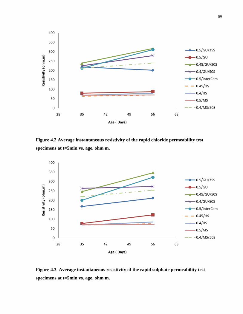
69
Figure 4.2 Average instantaneous resistivity of the rapid chloride permeability test
specimens at t=5min vs. age, ohm∙m.
Figure 4.3 Average instantaneous resistivity of the rapid sulphate permeability test
specimens at t=5min vs. age, ohm∙m.
0
50
100
150
200
250
300
350
400
28 35 42 49 56 63
Resi
stiv
ity (o
hm.m
)
Age ( Days)
0.5/GU/35S
0.5/GU
0.45/GU/50S
0.4/GU/50S
0.5/InterCem
0.45/HS
0.4/HS
0.5/MS
0.4/MS/50S
0
50
100
150
200
250
300
350
400
28 35 42 49 56 63
Resi
stiv
ity (o
hm.m
)
Age ( Days)
0.5/GU/35S
0.5/GU
0.45/GU/50S
0.4/GU/50S
0.5/InterCem
0.45/HS
0.4/HS
0.5/MS
0.4/MS/50S

70
With the exception of 2 mixtures (the chloride exposed 0.5/GU/35S specimens and the sulphate
exposed 0.4/GU/50S specimens at 35 days), all the resistivity values increased with age.
Initial (or pre – test) instantaneous resistivities may be separated into two groups of mixtures,
ones containing slag and fly ash and others containing 100% cement, where the highest
resistivity values are seen with the first group of mixtures. Thereby, demonstrating the ability of
using resistivity measurements to rapidly distinguish between concretes containing 100% cement
and concretes with either slag or fly ash cement replacements, and therefore, to some extent
identify high quality concrete.
Table 4.11 and Table 4.12 present the differences in the instantaneous resistivities at 5 minutes
for selected mixtures to highlight the effects of using GU cement vs. using HS and MS cement
types, water to cementing materials ratio and slag replacement. With respect to the effect of
cement type, for the same mix design, specimens containing GU cement, show higher initial
resistivity than those containing MS cement. Moreover, the 0.5/GU mix had higher resistivity
values than the 0.4/HS of the lower water to cement ratio, demonstrating that the difference in
cement type had a greater influence on resistivity values than the reduction of the w/cm from 0.5
to 0.4.
Note that in this case, at 5 minutes into the migration test, it is assumed that very negligible
amount of chemical binding has occurred. Therefore, it is reasonable to state that any changes
with respect to cement type at this stage may be attributed to the differences in the C2S contents
of the cements, rather than both the C2S and C3A contents. Also note that with the exception
0.5/GU mix at 56 days, the average 6 hours resistivity values of the specimens exposed to
sulphate were in all cases higher than the instantaneous resistivity measured at t = 5 minutes.
This trend is not seen with the chloride-exposed specimens as the resistivity values of these
specimens in some cases increased and in other cases decreased following the tests, overall,
following the 6 hour chloride exposure, the resistivity values specimens did not vary as much as
the resistivity of the sulphate-exposed specimens.
The variation in resistivity values of both the chloride and sulphate exposed specimens following
the migration tests could be either due to effects of chemical binding (especially sulphate which
had increased resistivity values), or due to leaching of ions out of the specimen into the
electrolyte and ingress of ions from the electrolyte into the specimen (thereby changing the pore

71
solution conductivity). It is important to remember that the conductivity of the specimens is
influenced by both the movements of the anions and cations. Therefore, in order to make
reliable conclusions with respect to this subject, it would be of interest to determine the
concentration of the ions in the pore solution compared to the concentration of the ions in the
electrolyte as well as determine the size of the capillary porosity of the specimens.
Unfortunately, pore solution extraction and porosity measurements were out of the scope of this
study, but are recommended for future related research.
Reducing the water to cement ratio from 0.4 to 0.45 did not significantly vary the resistivity
values of the two mixtures, however, the percent difference between them increased with age.
The effect of slag on the other hand, is seen clearly as the on average, the resistivity values of the
0.5/GU/35S mix are greater than those of the 0.5/GU mix by 60% and 48%, for the chloride and
sulphate exposed specimens, respectively. Also, the percent difference decreases with age and is
greater for the specimens exposed to chlorides.
Table 4.11 Differences between the instantaneous resistivities at =5min for selected
mixtures. Rapid chloride permeability test specimens.
𝑴𝒊𝒙 #𝟏−𝑴𝒊𝒙 #𝟐
𝝆�𝑵𝒂𝑪𝒍,@𝟓𝒎𝒊𝒏 𝒐𝒇 𝑴𝒊𝒙 #𝟏− 𝝆�𝑵𝒂𝑪𝒍,@𝟓𝒎𝒊𝒏 𝒐𝒇 𝑴𝒊𝒙 #𝟐
(ohm.m)
% 𝑫𝒊𝒇𝒇𝒆𝒓𝒆𝒏𝒄𝒆
= �𝝆�𝑵𝒂𝑪𝒍,@𝟓𝒎𝒊𝒏𝒐𝒇 𝑴𝒊𝒙 #𝟏 − 𝝆�𝑵𝒂𝑪𝒍,@𝟓𝒎𝒊𝒏𝒐𝒇 𝑴𝒊𝒙 #𝟐
𝝆�𝑵𝒂𝑪𝒍,@𝟓𝒎𝒊𝒏 𝒐𝒇 𝑴𝒊𝒙 #𝟏 �
× 𝟏𝟎𝟎% Age Age
35 days 56 days 35 Days 56 Days Effect of GU vs. MS and HS cements types
0.4/GU/50S - 0.4/MS/50S 12 39 5% 14%
0.5/GU - 0.5/MS 11 19 14% 22%
0.5/GU - 0.4/HS 11 9 14% 10%
Effect of water to cement ratio 0.45/GU/50S -
0.4/GU/50S 14 37 6% 12%
0.45/HS - 0.4/HS -5 -9 -8% -13%
Effect of Slag Replacement 0.5/GU/35S -
0.5/GU/ 139 113 64% 56%

72
Table 4.12 Differences between the instantaneous resistivities at =5min for selected
mixtures. Rapid sulphate permeability test specimens.
𝑴𝒊𝒙 #𝟏−𝑴𝒊𝒙 #𝟐
𝝆�𝑵𝒂𝟐𝑺𝑶𝟒,@𝟓𝒎𝒊𝒏 𝒐𝒇 𝑴𝒊𝒙 #𝟏− 𝝆�𝑵𝒂𝟐𝑺𝑶𝟒,@𝟓𝒎𝒊𝒏 𝒐𝒇 𝑴𝒊𝒙 #𝟐
(ohm.m)
% 𝑫𝒊𝒇𝒇𝒆𝒓𝒆𝒏𝒄𝒆
= �𝝆�𝑵𝒂𝟐𝑺𝑶𝟒,@𝟓𝒎𝒊𝒏𝒐𝒇 𝑴𝒊𝒙 #𝟏 − 𝝆�𝑵𝒂𝟐𝑺𝑶𝟒,@𝟓𝒎𝒊𝒏𝒐𝒇 𝑴𝒊𝒙 #𝟐
𝝆�𝑵𝒂𝟐𝑺𝑶𝟒,@𝟓𝒎𝒊𝒏 𝒐𝒇 𝑴𝒊𝒙 #𝟏�
× 𝟏𝟎𝟎% Age Age
35 days 56 days
35 Days 56 Days
Effect of GU vs. MS and HS cements types 0.4/GU/50S
- 0.4/MS/50S
45 19 17% 7%
0.5/GU - 0.5/MS 6 51 8% 41%
0.5/GU - 0.4/HS 7 39 9% 32%
Effect of water to cement ratio 0.45/GU/50S
- 0.4/GU/50S
-17 73 -7% 21%
0.45/HS - 0.4/HS -1 -9 1% 12%
Effect of Slag Replacement 0.5/GU/35S
- 0.5/GU/
91 89 54% 42%
Since the resistivity values were recorded at such an early stage in the tests when chemical
binding effect is negligible, the values of specimens belonging to the same mix were similar
regardless of the exposure solution. With the exception of the 0.5/GU/35S and 0.4/GU/50S
mixtures at 35 days and the 0.5/GU mix at 56 days, the percent differences between the sulphate-
exposed and chloride-exposed specimens instantaneous 5 minute resistivity, presented in Table
4.13, were less than 10%. Furthermore, with the exception of the 0.5/GU/35S and 0.5/InterCem
at 35 days and the 0.4/GU/50S at 56 days, the 5 minutes instantaneous resistivity values of the
sulphate-exposed specimens were in all cases higher than the resistivity values of the chloride
exposed specimens. As discussed in Section 2.10.1, it was expected that the conductivity of the
sodium sulphate-exposed specimens would be higher than the sodium chloride-exposed
specimens, however, since (with few exceptions) the percent differences were less than 10%, it is
reasonable to state that relative to the other variables investigated in this study, the effect of the
electrolyte solution did not greatly influence the rapid permeability test results.

73
Table 4.13 Percent difference between the instantaneous resistivity values of the sulphate
and chloride exposed specimens, measured at t = 5 minutes.
Mix ID
% 𝐃𝐢𝐟𝐟𝐞𝐫𝐞𝐧𝐜𝐞 =𝝆 𝑵𝒂𝟐𝑺𝑶𝟒@ 𝟓𝒎𝒊𝒏 − 𝝆 𝑵𝒂𝑪𝒍@ 𝟓𝒎𝒊𝒏
𝝆 𝑵𝒂𝟐𝑺𝑶𝟒@ 𝟓𝒎𝒊𝒏 × 𝟏𝟎𝟎%
Age
35 days 56 days
0.5/GU/35S -30 5
0.5/GU -3 28
0.45/GU/50S 3 9
0.4/GU/50S 14 -2
0.5/InterCem -6 3
0.45/HS 7 7
0.4/HS 3 6
0.5/MS 4 4
0.4/MS/50S 3 6
4.4 Rapid Migration Tests- NT Build 492
4.4.1 Penetration Depths As discussed in Chapter 3, once the concrete specimens were split and stained with the
appropriate indicators, the depths of penetration were measured visually. The depths of
penetration are influenced by the test voltage and therefore not all specimens can be compared
directly to each other. Test voltage affects the amount of ions being driven into the exposed
surface of the specimen per specific time period, for instance, assuming the resistivity of a
concrete samples remains constant for a specified time period, higher test voltage means higher
current and thus larger amounts of either sulphate or chloride ions attempting to penetrate into
the exposed face of the sample. Therefore, unless specimens were tested under the same voltage,
their depths of penetrations cannot be compared directly. To overcome this issue, all the
penetration depths were divided by their test voltages. The measured penetration depths, test
voltages, and their ratios at 35 and 56 days are presented in Table 4.14 to Table 4.17 and are
summarized in Figure 4.4.

74
Table 4.14 Measured penetration depths of specimens exposed to chlorides at 35 days
Mix ID
Chloride Exposed Specimens
Age: 35 days
Test Voltage
(V)
Specimen 1
(mm)
Specimen 2
(mm)
Average Penetration
Depth ( mm)
𝐀𝐯𝐞𝐫𝐚𝐠𝐞 𝐏𝐞𝐧𝐞𝐭𝐫𝐚𝐭𝐢𝐨𝐧 𝐃𝐞𝐩𝐭𝐡𝐓𝐞𝐬𝐭 𝐕𝐨𝐥𝐭𝐚𝐠𝐞
(mm/V)
0.5/GU/35S 35 11 18 14 0.4 0.5/GU 25 25 24 25 1.0
0.45/GU/50S 40 10 18 14 0.4 0.4/GU/50S 40 10 9 10 0.3
0.5/InterCem 40 19 20 19 0.5 0.45/HS 25 29 29 29 1.2 0.4/HS 25 23 22 22 0.9 0.5/MS 25 34 31 32 1.3
0.4/MS/50S 40 9 27 18 0.5
Average 20.3 0.7
Table 4.15 Measured penetration depths of specimen exposed to sodium chloride at 56 days
Mix ID
Chloride Exposed Specimens
Age: 56 days
Test Voltage
(V)
Specimen 1
(mm)
Specimen 2
(mm)
Average Penetration
Depth ( mm)
𝐀𝐯𝐞𝐫𝐚𝐠𝐞 𝐏𝐞𝐧𝐞𝐭𝐫𝐚𝐭𝐢𝐨𝐧 𝐃𝐞𝐩𝐭𝐡𝐓𝐞𝐬𝐭 𝐕𝐨𝐥𝐭𝐚𝐠𝐞
(mm/V)
0.5/GU/35S 40 14 13 13 0.3 0.5/GU 30 24 24 24 0.8
0.45/GU/50S 50 11 16 13 0.3 0.4/GU/50S 50 10 13 11 0.2
0.5/InterCem 50 14 20 17 0.3 0.45/HS 25 25 25 25 1.0 0.4/HS 30 21 21* 21 0.7 0.5/MS 25 37 36 37 1.5
0.4/MS/50S 40 9 10 10 0.3
Average 19 0.6
*tested at 25 V

75
Table 4.16 Measured penetration depths of specimen exposed to sulphates at 35 days
Mix ID
Sulphate Exposed Specimens
Age: 35 days
Test Voltage
(V)
Specimen 1
(mm)
Specimen 2
(mm)
Average Penetration
Depth ( mm)
𝐀𝐯𝐞𝐫𝐚𝐠𝐞 𝐏𝐞𝐧𝐞𝐭𝐫𝐚𝐭𝐢𝐨𝐧 𝐃𝐞𝐩𝐭𝐡𝐓𝐞𝐬𝐭 𝐕𝐨𝐥𝐭𝐚𝐠𝐞
(mm/V)
0.5/GU/35S 40 2.2 2.1 2.1 0.053 0.5/GU 25 3.6 3.7 3.6 0.144
0.45/GU/50S 40 1.8 1.3 1.5 0.038 0.4/GU/50S 40 1.0 1.2 1.1 0.028
0.5/InterCem 40 1.7 1.8 1.8 0.045 0.45/HS 25 2.2 1.7 2.0 0.080 0.4/HS 25 1.2 0.9 1.1 0.044 0.5/MS 25 2.8 2.4 2.6 0.104
0.4/MS/50S 40 1.4 1.2 1.3 0.033
Average 1.9 0.063
Table 4.17 Measured penetration depths of specimen exposed to sulphates at 56 days
Mix ID
Sulphate Chloride Exposed Specimens
Age: 56 days
Test Voltage
(V)
Specimen 1
(mm)
Specimen 2
(mm)
Average Penetration
Depth ( mm)
𝐀𝐯𝐞𝐫𝐚𝐠𝐞 𝐏𝐞𝐧𝐞𝐭𝐫𝐚𝐭𝐢𝐨𝐧 𝐃𝐞𝐩𝐭𝐡𝐓𝐞𝐬𝐭 𝐕𝐨𝐥𝐭𝐚𝐠𝐞
(mm/V)
0.5/GU/35S 40 1.3 1.3 1.3 0.033 0.5/GU 30 1.6 2.3 2.0 0.067
0.45/GU/50S 50 1.4 1.3 1.3 0.026 0.4/GU/50S 50 1.1 1.0 1.1 0.022
0.5/InterCem 50 1.2 1.6 1.4 0.028 0.45/HS 25 1.9 2.8 2.3 0.092 0.4/HS 30 2.0 1.7 1.8 0.060 0.5/MS 25 3.1 3.9 3.5 0.140
0.4/MS/50S 40 0.8 0.9 0.9 0.023
Average 1.7 0.055

76
The most obvious observation is the difference in depths of penetration of specimens exposed to
chlorides and those exposed to sulphates. As may be observed from Table 4.18, on average,
chloride penetration depths were between 6.7 to 20 times larger than sulphate penetration depths
at 35 days and between 10 to 12.1 times larger at 56 days. Overall, chloride penetration depths
were approximately 11 times greater than sulphate.
Note from Figure 4.14 to 4.17 that all the chloride penetration depth to test voltage ratios
decreased with age, whereas, the sulphate penetration depth to test voltage ratios decrease only
for the GU mixtures. Since the sulphate penetration depths were very small and since it was
more difficult to identify the sulphate fronts for specimens with HS and MS cements than for
specimens with GU cements, it is not known whether the difference in penetration fronts was due
to these issues or due to material variables. This is also applicable to Table 4.18, where the ratios
of the average chloride penetration depth to the average sulphate penetration depth increased
with age for all the specimens containing GU cement while the ratios of the mixtures containing
the HS and MS cements decreased with age.
Table 4.18 Average chloride to sulphate penetration depths ratios
Mix ID
𝑨𝒗𝒆𝒓𝒂𝒈𝒆 𝑪𝒍− 𝒑𝒆𝒏𝒆𝒕𝒓𝒂𝒕𝒊𝒐𝒏 𝒅𝒆𝒑𝒕𝒉 (𝒎𝒎)𝑨𝒗𝒆𝒓𝒂𝒈𝒆 𝑺𝑶𝟒
𝟐− 𝒑𝒆𝒏𝒆𝒕𝒓𝒂𝒕𝒊𝒐𝒏 𝒅𝒆𝒑𝒕𝒉 (𝒎𝒎)
Age
35 Days 56 Days
0.5/GU/35S 6.7 10.0 0.5/GU 6.9 12.0
0.45/GU/50S 9.3 10.0 0.4/GU/50S 9.1 10.0
0.5/InterCem 10.6 12.1 0.45/HS 14.5 10.9 0.4/HS 20.0 11.7 0.5/MS 12.3 10.6
0.4/MS/50S 13.8 11.1
Average 11.5 10.9

77
Figure 4.4 Comparison of SO42- and Cl- penetration depths at 35 and 56 days while accounting
for test voltage.
Another observation from Figure 4.4 and Table 4.14 to Table 4.17, is regarding the influence of
w/cm and slag replacement. As expected, mixtures with lower w/cm and with higher slag
replacements had lower depths of penetrations both for chloride and sulphate.
Also observed from Figure 4.4, is the effect of cement type on penetration depth. The chloride
penetration depths of specimens containing GU cements, with 10.7% C3A and 28% C2S, are
lower than the chloride penetration depths of the specimens containing MS, with 5.5% C3A and
14% C2S, of the same mix design. Thus, reinforcing that higher C2S and C3A contents decrease
diffusion rates. However, it is not known whether the difference in penetration depths is due a
higher degree of hydration (due to high C2S content) or due to higher chloride binding capacity
(due to high C3A content) in the GU cement specimens.
Prior to making observations and drawing conclusions with respect to the sulphate depths of
penetration, it is important to note, that it is rather difficult to differentiate between the different
mixtures and draw reliable conclusions, since the range of sulphate depths of penetration is very
small (never higher than 4 mm) and since the measurement is done visually. Furthermore, the
barium chloride, potassium permanganate dye gave different results for mixtures containing
100% cement than those containing slag as will be discussed below.
0
0.2
0.4
0.6
0.8
1
1.2
1.4
1.6
Aver
age
Pene
trat
ion
Dept
h /T
est V
olta
ge
(mm
/V)
Na2SO4 35 Days Na2SO4 56 Days NaCl 35 Days NaCl 56 Days

78
4.4.1.1 Observations Specific to the Sulphate Fronts
In order to identify the sulphate fronts, it was necessary to use a colorimetric method such as the
one used to identify chloride fronts by applying AgNO3 solution. Spraying silver nitrate on split
concrete specimens that had been exposed to chlorides results in white precipitation of silver
chloride on the depths to which chlorides have penetrated (Tang & Nilsson, 1992; Otsuki et al.,
1993). Similarly, the addition of sulphate ions to an aqueous solution of barium chloride results
in precipitation of barium sulphate. However, barium sulphate precipitate is not as distinct in
colour as silver chloride. Therefore, potassium permanganate was added to the barium chloride
solution, such that the permanganate co-precipitates with the barium sulphate, turning it purple
(Poole & Thomas, 1975).
Applying potassium permanganate, barium chloride solution to the split sulphate-exposed
specimens, allowed the measurement of the sulphate fronts as these turned purple. However,
regardless of the difficulty of measuring the fronts due their small penetrations depths (which
never exceeded 4 mm in the 24 hour long tests), the sulphate fronts of the mixtures containing
slag were much more distinct and therefore easier to measure. The penetration fronts of the slag
mixtures showed higher colour intensity and the boundary where the colour change was much
clearer than for the 100% cement mixtures, which on the other hand, showed smudged
boundaries and in some cases lower intensity in colour. Also for the original test duration, it was
more difficult to identify the sulphate fronts of the specimens containing 100% HS and MS
cements than the sulphate fronts of the specimens containing 100% GU cement.
The observations made with respect to the chloride and sulphate fronts are illustrated in Figure
4.5 to Figure 4.16. Note that for the 24 hour long tests, each pair of the sulphate and chloride
exposed specimens were cut from the same cylinder. In addition, note that extending the duration
of the modified NT Build 492 from 1 to 4 and 9 days increased the sulphate fronts, facilitating
the measurements. The results of the modified NT Build 492 tests with longer durations are
discussed in Section 4.4.3.

79
Figure 4.5 Sulphate penetration front of a 56 days old concrete specimen of 0.45 w/cm and
100% HS cement, tested in NT Build 492 testing conditions for 24 hours.
Figure 4.6 Chloride penetration front of a 56 days old concrete specimen of 0.45 w/cm and
100% HS cement, tested in NT Build 492 for 24 hours.

80
Figure 4.7 Sulphate penetration front of a 35 days old concrete specimen of 0.5 w/cm and
100% MS cement, tested in NT Build 492 testing conditions for 24 hours.
Figure 4.8 Chloride penetration front of a 35 days old concrete specimen of 0.5 w/cm and
100% MS cement, tested in NT Build 492 for 24 hours.

81
Figure 4.9 Sulphate penetration front of a 35 days old concrete specimen of 0.4 w/cm, MS
cement and 50% slag replacement, tested in NT Build 492 testing conditions for 24 hours.
Figure 4.10 Chloride penetration front of a 35 days old concrete specimen of 0.4 w/cm, MS
cement and 50% slag replacement, tested in NT Build 492 for 24 hours.

82
Figure 4.11 Sulphate penetration front of a 6.5 months old concrete specimen of 0.5 w/cm,
GU cement and 35 % slag replacement, tested in NT Build 492 testing conditions for 24
hours.
Figure 4.12 Sulphate penetration front of a 6.5 months old concrete specimen of 0.5 w/cm
and 100% GU cement, tested in NT Build 492 testing conditions for 24 hours.

83
Figure 4.13 Sulphate penetration front of a 6.5 months old concrete specimen of 0.5 w/cm,
GU cement and 35 % slag replacement, tested in NT Build 492 testing conditions for 4
days.
Figure 4.14 Sulphate penetration front of a 6.5 months old concrete specimen of 0.5 w/cm
and 100% GU cement, tested in NT Build 492 testing conditions for 4 days.

84
Figure 4.15 Sulphate penetration front of a 6.5 month old concrete specimen of 0.5 w/cm,
GU cement with 35% slag replacement, tested in NT Build 492 testing conditions for 9
days.
Figure 4.16 Sulphate penetration front of a 6.5 month old concrete specimen of 0.5 w/cm
and 100% GU cement, tested in NT Build 492 testing conditions for 9 days.

85
In order to verify that the front that is stained does in fact contain sulphates from external
sources, 2 specimens of different mixtures were profile ground after they were split and stained
and sent for ICP chemical analysis to determine the sulphur levels at each layer. The results are
presented Section 3.3.2.5 .
4.4.1.2 Chloride Migration Coefficient
The non-steady state chloride migration coefficients, 𝐷𝑁𝑎𝐶𝑙,𝑛𝑠𝑠𝑚, were calculated using the
following equation available in the NT Build 492 standard:
𝐷𝑁𝑎𝐶𝑙,𝑛𝑠𝑠𝑚 =0.0239(273 + 𝑇)𝐿
(𝑈 − 2)𝑡�𝑥𝑑 − 0.0238�
(273 + 𝑇)𝐿𝑥𝑑𝑈 − 2
� Eq. 4.1
Where DNaCl,nssm is the non-steady-state chloride migration coefficient, x10-12 m2/s; U is the
absolute values of the applied voltage, V; T is the average values of the initial and final
temperatures in the anolyte solution, °C; L is the thickness of the specimen, mm; Xd is the
average values of penetration depths, mm; t is the test duration, hours.
The calculated chloride migration tests are presented in Table 4.19. The initial observation is the
decrease of the chloride migration coefficient with age for all but for the 0.5/MS mix (which had
higher than expected penetration depths). As well, the effect of fly ash is evident as the
migration coefficient of the fly ash blended cement mix, 0.5/InterCem, decreased steeply from an
average migration coefficient of 7.2x10⁻¹² m2/s at 35 days to 4.6 x10⁻¹² m2/s at 56 days. A
comparison among mixtures containing the same cement types shows lower migration
coefficients for mixtures with lower water to cement ratios and higher slag replacements.
Furthermore, as with the rapid permeability test results, the chloride migration coefficients may
be separated into two groups: one containing the mixtures with 100% cement and another
containing the mixtures with slag and fly ash.

86
Table 4.19 Summary of chloride migration coefficients, NT Build 492
Mix ID
Chloride migration coefficient, 𝑫𝑵𝒂𝑪𝒍 , x 10-12 (m2/s) % 𝑫𝒊𝒇𝒇𝒆𝒓𝒆𝒏𝒄𝒆
= �𝑫�𝑵𝒂𝑪𝒍@ 𝟑𝟓 𝒅𝒂𝒚𝒔 − 𝑫�𝑵𝒂𝑪𝒍 @ 𝟓𝟔 𝒅𝒂𝒚𝒔
𝑫�𝑵𝒂𝑪𝒍,𝒏𝒔𝒔𝒎 @ 𝟑𝟓 𝒅𝒂𝒚𝒔 �
× 𝟏𝟎𝟎%
Age: 35 days Age: 56 days
Spec 1
Spec 2 Avg Spec
1 Spec
2 Avg
0.5/GU/35S 4.4 7.1 5.7 5.0 4.6 4.9 14 % 0.5/GU 13.8 13.4 13.6 11.2 11.0 11.1 18%
0.45/GU/50S 3.3 6.3 4.8 2.9 4.5 3.7 23% 0.4/GU/50S 3.4 3.1 3.2 2.7 3.3 3.0 6%
0.5/InterCem 7.2 7.2 7.2 3.9 5.4 4.6 36% 0.45/HS 16.9 16.7 16.8 14.2 14.1 14.1 16% 0.4/HS 12.9 12.5 12.7 9.9 11.8 10.8 15% 0.5/MS 19.6 17.7 18.7 21.4 20.9 21.2 -13%
0.4/MS/50S 2.9 9.5* 6.2 2.9 3.2 3.1 50% * Note that the penetration depths of this specimen were higher than expected, resulting in a high
migration coefficient.
Table 4.20 summarizes the differences between the chloride migration coefficients of selected
mixtures to demonstrate the influence of using GU cement vs. using HS and MS cement types,
w/cm and slag replacement on the migration coefficients.
With respect to the effect of the cement type on the chloride migration coefficient, both mixtures
containing GU cement, 0.5/GU and 0.4/GU/50S, had lower migration coefficients than the MS
mixtures, 0.5/MS and 0.4/GU/50S of the same mix designs. Furthermore, the 0.5/GU mixture
had lower migration coefficient than the 0.45/HS mixture, of the lower w/cm, demonstrating that
the difference in cement type had a greater influence on the migration coefficient than the
reduction of the w/cm from 0.5 to 0.45.
If the migration coefficient obtained from specimen 2 of the 0.4/MS/50S mix at 35 days is
disregarded, its chloride migration coefficient would be very similar to that of the 0.4/GU/50S
mix.

87
Table 4.20 Differences between chloride migration coefficients for selected mixtures
𝑴𝒊𝒙#𝟏−𝑴𝒊𝒙#𝟐
𝑫�𝑵𝒂𝟐𝑺𝑶𝟒 𝒐𝒇 𝑴𝒊𝒙 #𝟏− 𝑫�𝑵𝒂𝟐𝑺𝑶𝟒𝒐𝒇 𝑴𝒊𝒙 #𝟐
× 𝟏𝟎−𝟏𝟐 (𝒎𝟐 𝒔⁄ )
% 𝑫𝒊𝒇𝒇𝒆𝒓𝒆𝒏𝒄𝒆
= �𝑫�𝑵𝒂𝟐𝑺𝑶𝟒 𝒐𝒇 𝑴𝒊𝒙 #𝟏 − 𝑫�𝑵𝒂𝟐𝑺𝑶𝟒𝒐𝒇 𝑴𝒊𝒙 #𝟐
𝑫�𝑵𝒂𝟐𝑺𝑶𝟒 𝒐𝒇 𝑴𝒊𝒙 #𝟏�
× 𝟏𝟎𝟎% Age Age
35 Days 56 Days 35 Days 56 Days
Effect of GU vs. MS and HS cements types
0.5/MS – 0.5/GU 5.12 10.07 27% 48%
0.4/MS/50S – 0.4/GU/50S 2.95 * 0.05 48% 2%
0.45/HS – 0.5/GU 3.23 3.05 19% 22%
Effect of Water to Cement Ratio 0.45/HS –
0.4/HS 4.07 3.32 24% 23%
0.45/GU/50S – 0.4/GU/50S 1.58 0.68 33% 18%
Effect of Slag Replacement 0.5/GU –
0.5/GU/35S 7.85 6.31 58% 57%
∗ 0.4/MS/50S shows the greatest range in migration coefficient at 35 days, due to higher than usual depth of penetration in one of the two specimens.
4.4.1.3 Sulphate Migration Coefficient
The non-steady state sulphate migration coefficients, 𝐷𝑁𝑎2𝑆𝑂4,𝑛𝑠𝑠𝑚 , were also calculated from
Equations 1 to 3 in the NT Build 492 standard:
𝐷𝑛𝑠𝑠𝑚 =𝑅𝑇𝑧𝐹𝐸
∙𝑥𝑑 − 𝛼�𝑥𝑑
𝑡 Eq. 4.2
Where:
𝐸 =𝑈 − 2𝐿
Eq. 4.3
𝛼 = 2�𝑅𝑇𝑧𝐹𝐸
∙ 𝑒𝑟𝑓−1 �1 −2𝑐𝑑𝑐0� Eq. 4.4

88
Dnssm is the non-steady-state migration coefficient, m2/s; z is the absolute value of ion valence for
sulphate z=2;F is the Faraday constant, F=9.648x10⁴ J/(V∙mol); U is the absolute value of the
applied voltage, V; R is the gas constant, R=8.314 J/(K∙mol); T is the average values of the
initial and final temperatures in the anolyte solution, K; L is the thickness of the specimen, m; Xd
is the average values of penetration depths, m; t is the test duration, seconds; erf-1 is the inverse
of error function; cd is the sulphate concentration by weight of concrete powder at which the
colour changes, cd ≈ 4.54 x 10⁻⁵ moles per gram of concrete powder; c0 is the sulphate
concentration in the catholyte solution, C0 ≈ 0704 moles. It follows then that the value of the
𝑒𝑟𝑓−1 �1 − 2𝑐𝑑𝑐0� term in Eq. 4.4 is equal to 2.7.
Table 4.21 summarizes all the calculated sulphate migration coefficients. With the exception of
the 0.45/HS, the 0.4/HS and the 0.5/Ms mixtures, all sulphate migration coefficient decrease with
age. This inconsistency is likely due to the very small and unclear depth of penetrations observed
with these mixtures. As well, for all the results discussed thus far, the lowest sulphate migration
coefficients are seen with the mixtures of the lower water to cement ratios and higher slag
replacements. At 35 days, the highest sulphate migration coefficient is seen with the 0.5/GU mix
and at 56 days the 0.5/MS mix has the highest coefficient. However, it is important to note that
the sulphate migration coefficients are highly sensitive to small differences in the depths of
penetration measurements, only because the depths of penetrations are on such a small scale.
Table 4.21 Summary of sulphate migration coefficients, modified NT Build 492 specimens.
Mix ID
Sulphate migration coefficient, x 10-12 (m2/s)
Age: 35 days Age: 56 days
Spec 1 Spec 2 Avg Spec 1 Spec 2 Avg
0.5/GU/35S 0.23 0.21 0.22 0.10 0.10 0.10
0.5/GU 0.59 0.63 0.61 0.15 0.28 0.22
0.45/GU/50S 0.16 0.09 0.13 0.10 0.09 0.09
0.4/GU/50S 0.06 0.08 0.07 0.07 0.06 0.06
0.5/InterCem 0.17 0.18 0.18 0.07 0.13 0.10
0.45/HS 0.28 0.18 0.23 0.20 0.41 0.31
0.4/HS 0.07 0.02 0.04 0.23 0.16 0.19
0.5/MS 0.43 0.33 0.38 0.48 0.69 0.58
0.4/MS/50S 0.10 0.08 0.09 0.04 0.04 0.04
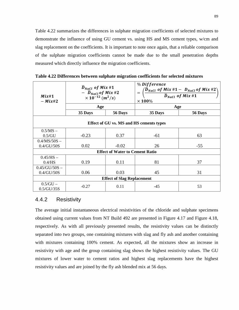
89
Table 4.22 summarizes the differences in sulphate migration coefficients of selected mixtures to
demonstrate the influence of using GU cement vs. using HS and MS cement types, w/cm and
slag replacement on the coefficients. It is important to note once again, that a reliable comparison
of the sulphate migration coefficients cannot be made due to the small penetration depths
measured which directly influence the migration coefficients.
Table 4.22 Differences between sulphate migration coefficients for selected mixtures
𝑴𝒊𝒙#𝟏−𝑴𝒊𝒙#𝟐
𝑫�𝑵𝒂𝑪𝒍 𝒐𝒇 𝑴𝒊𝒙 #𝟏− 𝑫�𝑵𝒂𝑪𝒍 𝒐𝒇 𝑴𝒊𝒙 #𝟐
× 𝟏𝟎−𝟏𝟐 (𝒎𝟐 𝒔⁄ )
% 𝑫𝒊𝒇𝒇𝒆𝒓𝒆𝒏𝒄𝒆
= �𝑫�𝑵𝒂𝑪𝒍 𝒐𝒇 𝑴𝒊𝒙 #𝟏 − 𝑫𝑵𝒂𝑪𝒍 𝒐𝒇 𝑴𝒊𝒙 #𝟐
𝑫�𝑵𝒂𝑪𝒍 𝒐𝒇 𝑴𝒊𝒙 #𝟏�
× 𝟏𝟎𝟎% Age Age
35 Days 56 Days 35 Days 56 Days
Effect of GU vs. MS and HS cements types
0.5/MS – 0.5/GU -0.23 0.37 -61 63
0.4/MS/50S – 0.4/GU/50S 0.02 -0.02 26 -55
Effect of Water to Cement Ratio 0.45/HS –
0.4/HS 0.19 0.11 81 37 0.45/GU/50S –
0.4/GU/50S 0.06 0.03 45 31 Effect of Slag Replacement
0.5/GU – 0.5/GU/35S -0.27 0.11 -45 53
4.4.2 Resistivity
The average initial instantaneous electrical resistivities of the chloride and sulphate specimens
obtained using current values from NT Build 492 are presented in Figure 4.17 and Figure 4.18,
respectively. As with all previously presented results, the resistivity values can be distinctly
separated into two groups, one containing mixtures with slag and fly ash and another containing
with mixtures containing 100% cement. As expected, all the mixtures show an increase in
resistivity with age and the group containing slag shows the highest resistivity values. The GU
mixtures of lower water to cement ratios and highest slag replacements have the highest
resistivity values and are joined by the fly ash blended mix at 56 days.

90
For the same mix design and even with the higher w/cm, mixtures containing GU cement, the
0.4/GU/50S and the 0.45/GU/50S mixtures, show higher resistivity than the MS cement mix,
0.4/MS/50S. The same trend is seen among the group of mixtures containing 100% cement,
where the 0.5/GU mix, although not having the lowest w/cm ratio has a resistivity higher than
the 100% HS and 100% MS mixtures, although the HS mix is of lower w/cm. It should be noted
however, that the differences in resistivity values are less among the 100% cement group of
mixtures.
Figure 4.17 Average instantaneous initial electrical resistivity of rapid chloride migration
test specimens vs. age, ohm∙m, (NT Build 492).
0
50
100
150
200
250
300
350
28 35 42 49 56 63
Resi
stiv
ity (o
hm.m
)
Age (Days)
0.5/GU/35S
0.5/GU
0.45/GU/50S
0.4/GU/50S
0.5/InterCem
0.45/HS
0.4/HS
0.5/MS
0.4/MS/50S

91
Figure 4.18 Average instantaneous initial electrical resistivity of rapid sulphate migration
specimens vs. age, ohm∙m, (modified NT Build 492).
Since the resistivity values were recorded at such an early stage in the tests when chemical
binding effect is negligible, the values of specimens belonging to the same mix were similar
regardless of the exposure solution. With the exception of the 0.5/GU/35S and 0.4/GU/50S
mixtures at 35 days and the 0.5/GU mix at 56 days, the percent differences between the sulphate-
exposed and chloride-exposed specimens instantaneous 5 minute resistivity, presented in Table
4.13, were less than 10%. Furthermore, with the exception of the 0.5/GU/35S and 0.5/InterCem
at 35 days and the 0.4/GU/50S at 56 days, the 5 minutes instantaneous resistivity values of the
sulphate-exposed specimens were in all cases higher than the resistivity values of the chloride
exposed specimens. As discussed in Section 2.10.1, it was expected that the conductivity of the
sodium sulphate-exposed specimens would be higher than the sodium chloride-exposed
specimens, however, since (with few exceptions) the percent differences were less than 10%, it is
reasonable to state that relative to the other variables investigated in this study, the effect of the
electrolyte solution did not greatly influence the rapid permeability test results.
Table 4.23 presents the percent difference between the instantaneous resistivity values of the
sulphate and chloride exposed specimens. Similar to the resistivity values measured from the
0
50
100
150
200
250
300
350
28 35 42 49 56 63
Resi
stiv
ity (o
hm.m
)
Age (Days)
0.5/GU/35S
0.5/GU
0.45/GU/50S
0.4/GU/50S
0.5/InterCem
0.45/HS
0.4/HS
0.5/MS
0.4/MS/50S

92
rapid permeability test, since the resistivity values were recorded at such an early stage in the
tests when chemical binding effect is negligible, the values of specimens belonging to the same
mix were similar regardless of the exposure solution. With the exception of the 0.5/GU/35S mix
at 35 days, the percent differences between the sulphate-exposed and chloride-exposed
specimens were less than 10%. Furthermore, the percent differences were lower than the percent
differences seen with the instantaneous resistivity values measured from the rapid permeability
tests at 5 minutes. Although the catholyte concentrations in the latter tests were lower and were
therefore expected to have lower impact on the differences. Therefore, as stated in Section 4.3.3,
relative to the other variables investigated in this study, it is reasonable to state that the effect of
the electrolyte solution did not greatly influence the rapid migration results.
Table 4.23 Percent difference between the instantaneous resistivity values of the sulphate
and chloride exposed specimens.
Mix ID
% 𝐃𝐢𝐟𝐟𝐞𝐫𝐞𝐧𝐜𝐞 =𝝆 𝑵𝒂𝟐𝑺𝑶𝟒@ 𝒕=𝟎 𝒎𝒊𝒏 − 𝝆 𝑵𝒂𝑪𝒍@ 𝒕=𝟎 𝒎𝒊𝒏
𝝆 𝑵𝒂𝟐𝑺𝑶𝟒@ 𝒕=𝟎 𝒎𝒊𝒏 × 𝟏𝟎𝟎%
Age
35 days 56 days
0.5/GU/35S 11.81 5.36
0.5/GU -0.18 -0.37
0.45/GU/50S 6.00 -1.95
0.4/GU/50S 0.07 2.76
0.5/InterCem 1.68 -0.45
0.45/HS 3.57 3.02
0.4/HS 3.29 5.98
0.5/MS 8.13 3.05
0.4/MS/50S 1.88 -4.89
4.4.3 Modified Test Length
Exposing the concrete specimens to sulphate migration tests for the original test time of 1 day
resulted in sulphate penetration depths which were not higher than 4 mm. Since the measurement
of the depths of penetration is visual, it was very difficult to distinguish between the depths of

93
penetrations of all the mixtures. As well, the relatively small sulphate fronts also translate into
higher variability in measured sulphate fronts due to the dependence of the measured depths on
the judgment of the tester. Therefore, 6.5 month old specimens of M1:0.5/GU/35S and
M2:0.5/GU (of different batches than those used for rapid migration and permeability tests) were
tested in the rapid migration test for longer periods of 1, 4 and 9 days. In addition to recording
the initial and final currents, the current of every specimen was recorded at an average of 5
minute intervals throughout the tests, enabling the determination of the total charge passing
through the sample, as well as the change in resistivity throughout the test length.
4.4.3.1 Total Charge Passing
During the NT Build 492 tests with the modified test durations, the current was recorded at
approximately 5 minutes intervals throughout the test duration, allowing for the determination of
the total charge passed by calculating the area under current vs. time plot using the trapezoidal
rule. The total charge passing through the 6.5 month old specimens are summarized in Table
4.24. As with the rapid sulphate penetration test (modified ASTM C1202) results, for the same
test length of 1 day, the total charge passing through the chloride specimens is greater than that
of the sulphate specimens and the difference is greater between the specimens which contain
slag. Regardless of the exposure solution, the total charge passing through the specimens
containing slag is lower than those with 100% cement, however the average difference decreases
with an increased test time as shown in Table 4.24. The relationships between the total charge
passed and test time are presented in Figure 4.19, the total charge passing increased linearly with
test time for both mixtures.
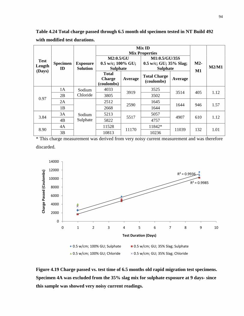
94
Table 4.24 Total charge passed through 6.5 month old specimen tested in NT Build 492
with modified test durations.
Test Length (Days)
Specimen ID
Exposure Solution
Mix ID Mix Properties
M2-
M1 M2/M1
M2:0.5/GU 0.5 w/c; 100% GU;
Sulphate
M1:0.5/GU/35S 0.5 w/c; GU; 35% Slag;
Sulphate Total
Charge (coulombs)
Average Total Charge (coulombs) Average
0.97
1A Sodium Chloride
4033 3919
3525 3514 405 1.12
2B 3805 3502 2A
Sodium Sulphate
2512 2590
1645 1644 946 1.57
1B 2668 1644
3.84 3A 5213
5517 5057
4907 610 1.12 4B 5822 4757
8.90 4A 11528
11170 11842*
11039 132 1.01 3B 10813 10236
* This charge measurement was derived from very noisy current measurement and was therefore
discarded.
Figure 4.19 Charge passed vs. test time of 6.5 months old rapid migration test specimens.
Specimen 4A was excluded from the 35% slag mix for sulphate exposure at 9 days- since
this sample was showed very noisy current readings.
R² = 0.9936
R² = 0.9985
0
2000
4000
6000
8000
10000
12000
14000
0 1 2 3 4 5 6 7 8 9 10
Char
ge P
asse
d (C
oulo
mbs
)
Test Duration (Days)
0.5 w/cm; 100% GU; Sulphate 0.5 w/cm; GU; 35% Slag; Sulphate
0.5 w/cm; 100% GU; Chloride 0.5 w/cm; GU; 35% Slag; Chloride

95
4.4.3.2 Penetration Depths
The measured penetration depths of the extended rapid migration tests are presented in Table
4.25, as well, the penetration depths of some of the specimens were illustrated in Figure 4.11 to
Figure 4.16 in Section 4.4.1.1. As with the original migration tests, chloride penetration depths
were significantly lower than those of sulphate. Chlorides penetrated over twice as deep into
specimens containing 100% cement than into specimens containing slag. The differences
between the sulphate penetration depths of these two mixtures were not as great. Furthermore,
the measured penetration depths of the specimens containing slag were greater than the
specimens containing 100% cement. However, it is important to note that the sulphate fronts
were very clear for the slag specimens but rather smudged with the 100% cement specimens,
reducing the reliability of the measurements of latter mix. Nonetheless, it was clear that the
sulphate penetration fronts increased with test length as presented in Table 4.25.
Table 4.25 Penetration depth of 6.5 month old specimens tested in original and modified
NT 492 for longer test durations.
Test Duration
(Days)
Specimen
ID
Exposure
Solution
Penetration Depth (mm) Mix ID
Mix Properties M2:0.5/GU
0.5 w/c; 100% GU
M1:0.5/GU/35S 0.5 w/c; GU; 35%
Slag
1
1A Sodium Chloride
15.0 6.6 2B 16.4 7.7 2A
Sodium Sulphate
1.5 1.0 1B 1.3 1.3
4 3A 2.3 3.1 4B 2.3 3.3
9 4A 4.6 4.2 3B 3.7 4.3
4.4.3.3 Migration Coefficients
The migration coefficients of the 6.5 months old specimens tested under longer test duration are
presented in Table 4.26. As with the migration coefficients of the original test duration discussed
in previous sections, the reliability of the calculated migration coefficients is directly related to
the reliability of the measurements of the penetration depth.

96
Table 4.26 Migration coefficients of the 6.5 months old specimens tested in the original and
modified NT Build 492 for longer test durations of 1, 4 and 9 days.
Test Length
(Days)
Specimen
ID
Exposure
Solution
Migration Coefficient, x10-12 (m2/s) Mix ID
Mix Properties M2:0.5/GU
0.5 w/c; 100% GU
M1:0.5/GU/35S 0.5 w/c; GU; 35%
Slag
1
1A Sodium Chloride
8.0 2.6 2B 8.7 3.2 2A
Sodium Sulphate
0.14 0.05 1B 0.10 0.09
4 3A 0.07 0.08 4B 0.07 0.09
9 4A 0.08 0.05 3B 0.06 0.05
4.4.3.4 Resistivity
Each line in Figure 4.20 to Figure 4.22 represents the change in resistivity throughout the
specified test duration, calculated from the recorded current values throughout the test and the
specimen dimensions. The resistivity of the sulphate specimens increased throughout all test
durations and in all cases, the resistivity of the slag mix was always greater than that of 100%
cement mix. The chloride resistivity on the other hand, remained almost constant throughout 24
hour long tests. These changes in resistivity values agree with the changes observed with the
rapid permeability and rapid migration tests.

97
Figure 4.20 Resistivity vs. test duration of the 6.5 months specimens tested in original and
modified NT Build 492 for the original test duration of 1 day.
Figure 4.21 Resistivity vs. test duration of the 6.5 months old specimens tested in the
modified NT Build 492 for 4 days.
0.5 w/c; 100% GU; Chloride
0.5 w/c; 100% GU; Sulphate
0.5 w/c; GU; 35% Slag; Chloride
0.5 w/c; GU; 35% Slag; Sulphate
0
100
200
300
400
500
600
700
800
900
1000
0 4 9 14 19 24 28
Resi
stiv
ity (O
hm.m
)
Test Duration (Hours)
0.5 w/c; 100% GU; Sulphate
0.5 w/c; GU; 35% Slag; Sulphate
0
100
200
300
400
500
600
700
800
900
1000
0 1 2 3 4 5
Resi
stiv
ity (O
hm.m
)
Test Duration (Days)
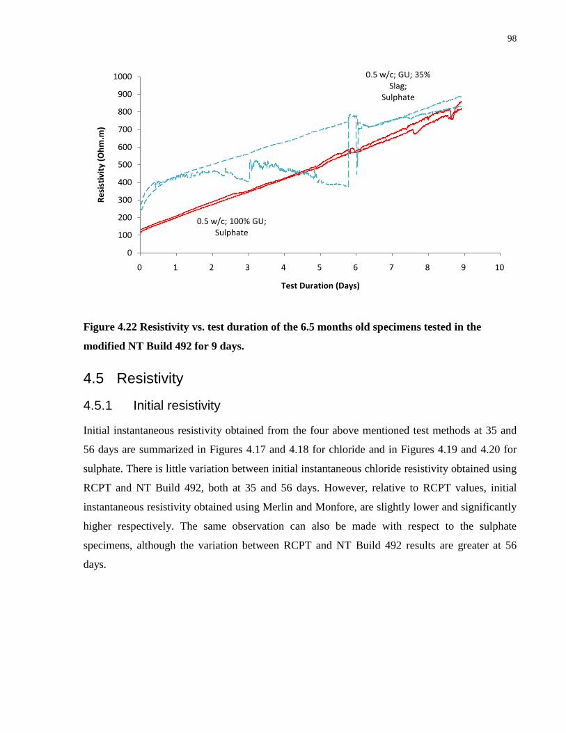
98
Figure 4.22 Resistivity vs. test duration of the 6.5 months old specimens tested in the
modified NT Build 492 for 9 days.
4.5 Resistivity
4.5.1 Initial resistivity
Initial instantaneous resistivity obtained from the four above mentioned test methods at 35 and
56 days are summarized in Figures 4.17 and 4.18 for chloride and in Figures 4.19 and 4.20 for
sulphate. There is little variation between initial instantaneous chloride resistivity obtained using
RCPT and NT Build 492, both at 35 and 56 days. However, relative to RCPT values, initial
instantaneous resistivity obtained using Merlin and Monfore, are slightly lower and significantly
higher respectively. The same observation can also be made with respect to the sulphate
specimens, although the variation between RCPT and NT Build 492 results are greater at 56
days.
0.5 w/c; 100% GU; Sulphate
0.5 w/c; GU; 35% Slag;
Sulphate
0
100
200
300
400
500
600
700
800
900
1000
0 1 2 3 4 5 6 7 8 9 10
Resi
stiv
ity (O
hm.m
)
Test Duration (Days)

99
Figure 4.23 Summary of initial resistivity values of chloride exposed specimens at 35 days
Figure 4.24 Summary of initial resistivity values of chloride exposed specimens at 56 days
0
50
100
150
200
250
300
350
400
450In
itial
Res
istiv
ity (o
hm.m
)
RCP:5 min NT 492 Merlin Monfore
0
50
100
150
200
250
300
350
400
450
Initi
al R
esis
tivity
(ohm
.m)
RCP:5 min NT 492 Merlin Monfore

100
Figure 4.25 Summary of initial resistivity values of sulphate exposed specimens at 35 days
Figure 4.26 Summary of initial resistivity values of sulphate exposed specimens at 56 days
0
50
100
150
200
250
300
350
400
450
Initi
al R
esis
tivity
(ohm
.m)
RCP:5 min NT 492 Merlin Monfore
0
50
100
150
200
250
300
350
400
450
Initi
al R
esis
tivity
(ohm
.m)
RSP:5 min NT 492 Merlin Monfore

101
4.5.2 Relationships between Merlin Resistivity, NT Build 492 and ASTM C 1202
The relationship between the initial Merlin bulk electrical resistivity and total ASTM C 1202
charge values is presented in Figure 4.27 and Figure 4.28 for specimens exposed to chloride and
sulphate, respectively. Also presented in these figures is the relationship of the resistivity
measured using from the ASTM C 1202 set up at t = 5 minutes. In both cases, an inverse
relationship is seen between the total charge and initial resistivity. In the case of the chloride
exposed specimen, the exponents are just above -1, while for the sulphate exposed specimens the
exponents are just below -1, thus it is reasonable to assume that all the exponents are equal to -1.
Moreover, since all the samples were tested for 6 hours, dividing the total charge by 6 hours will
give the average 6 hour current and the trend will remain the same. Therefore, the relationship
between the total charge and resistivity is: 𝑄 = 𝐶𝑜𝑛𝑠𝑡𝑎𝑛𝑡 ∙ 1𝑅, dividing Q by 6 hours: 𝐼6̅ℎ𝑟𝑠 =
𝐶𝑜𝑛𝑠𝑡𝑎𝑛𝑡 ∙ 6 ℎ𝑟𝑠 ∙ 1𝑅. That is, the trend observed is similar to trend suggested by ohm’s law,
I=V/R. Reinforcing that resistivity tests can be used as indicators of the quality of concrete,
similar to the RCPT.
To verify the accuracy of the above mentioned assumption, the data in Figure 4.27 and Figure
4.28 was re-plotted and presented in Figure 4.29 and Figure 4.30 while assuming that the total
charge passing and the measured resistivity are inversely proportional. As may observed, the
assumption was successfully verified as linear relationships with R2 values both very close to 1
and to the R2 values in Figure 4.27 and Figure 4.28. Although, there were better fits at lower
resistivity values.

102
Figure 4.27 Total 6 hour rapid chloride permeability test charge vs. instantaneous initial
resistivity.
Figure 4.28 Total 6 hour rapid sulphate permeability test charge vs. instantaneous initial
resistivity.
y = 158993x-1.015
R² = 0.9919
y = 302097x-1.089
R² = 0.981
0
500
1000
1500
2000
2500
3000
3500
4000
0 50 100 150 200 250 300 350 400 450
QRC
PT, 6
hr
(cou
lom
bs)
Resistivity (ohm.m)
Initial Merlin Resistivity RCPT Insantaneous Resistivity at t = 5 min
y = 73085x-0.899
R² = 0.9811
y = 138725x-0.972
R² = 0.9899
0
500
1000
1500
2000
2500
3000
0 50 100 150 200 250 300 350 400 450
QRC
PT, 6
hr
(cou
lom
bs)
Resistivity (ohm.m)
Initial Merlin Resistivity RCPT Insantaneous Resistivity at t = 5 min
cOutlier

103
Figure 4.29 Total 6 hour rapid chloride permeability test charge vs. inverse instantaneous
initial resistivity.
Figure 4.30 Total 6 hour rapid chloride permeability test charge vs. inverse instantaneous
initial resistivity.
y = 154380x - 48.532R² = 0.9901
y = 220728x - 157.7R² = 0.99
0
500
1000
1500
2000
2500
3000
3500
4000
0 0.005 0.01 0.015 0.02 0.025
QRC
PT, 6
hr
(cou
lom
bs)
Resistivity-1 (ohm-1.m-1)
Initial Merlin Resistivity RCPT Insantaneous Resistivity at t = 5 min
y = 102819x + 119.7R² = 0.9708
y = 155842x + 20.409R² = 0.9852
0
500
1000
1500
2000
2500
3000
0 0.005 0.01 0.015 0.02 0.025
QRC
PT, 6
hr
(cou
lom
bs)
Resistivity-1 (ohm-1.m-1)
Initial Merlin Resistivity RCPT Insantaneous Resistivity at t = 5 min
cOutlier

104
Figure 4.31 to Figure 4.34 present the relationships between the initial Merlin Resistivity, the
instantaneous resistivity measured from ASTM C1202 at t = 5 minutes and initial instantaneous
NT Build 492 resistivity. In all cases a linear relationship is seen, although a better fit is seen at
lower resistivity values. For the same specimens, Merlin resistivities were on average:
1. 23% lower than the resistivities measured from the original ASTM C 1202.
2. 27% lower than the resistivities measured from the modified ASTM C 1202.
3. 22% lower than the resistivities measured from the original NT Build 492.
4. 23% lower than the resistivities measured from the modified NT Build 492.
Figure 4.31 Instantaneous resistivity at t = 5 min vs. initial Merlin resistivity, rapid chloride
permeability test specimens.
y = 1.1445x + 12.675R² = 0.9933
0
50
100
150
200
250
300
350
0 50 100 150 200 250 300
Inst
anta
neou
s RCP
T Re
sist
ivity
at t
= 5
min
(o
hm.m
)
Initial Merlin Resistivity (ohm.m)
Outliers

105
Figure 4.32 Instantaneous resistivity at t = 5 min vs. initial Merlin resistivity, rapid
sulphate permeability test specimens.
Figure 4.33 Instantaneous initial NT Build 492 resistivity vs. initial Merlin resistivity.
Sodium chloride exposed specimens.
y = 1.2165x + 12.17R² = 0.9764
0
50
100
150
200
250
300
350
400
450
0 50 100 150 200 250 300
Inst
anta
neou
s RCP
T Re
sist
ivity
at t
= 5
min
(o
hm.m
)
Initial Merlin Resistivity (ohm.m)
y = 1.1668x + 10.634R² = 0.9777
0
50
100
150
200
250
300
350
400
450
0 50 100 150 200 250 300
Inst
anta
neou
s Ini
tial R
esis
tivity
N
T Bu
ild 4
92 (o
hm.m
)
Initial Merlin Resistivity (ohm.m)
Outlier
Outlier

106
Figure 4.34 Instantaneous initial NT Build 492 resistivity vs. initial Merlin resistivity.
Sodium sulphate exposed specimens.
Figures 4.27 to 4.28 present the relationships between chloride and sulphate migration
coefficients and initial Merlin resistivity. As may be observed, specimens of lower Merlin
resistivity values had a large range of migration coefficients leading to an unsatisfactory fits
either inverse nor bilinear functions and an inability of predicting the diffusion coefficient from
these low ranges of Merlin resistivities.
y = 1.1494x + 14.564R² = 0.981
0
50
100
150
200
250
300
350
400
450
0 50 100 150 200 250 300
Inst
anta
neou
s Ini
tial R
esis
tivity
NT
Build
492
(ohm
.m)
Initial Merlin Resistivity (ohm.m)

107
Figure 4.35 Chloride migration coefficients vs. initial Merlin resistivity
Figure 4.36 Sulphate migration coefficients vs. initial Merlin resistivity.
y = 685.11x-0.969
R² = 0.8646
0
5
10
15
20
25
0 50 100 150 200 250 300
Chlo
ride
Mig
ratio
n Co
effic
ient
, x10
-12
(m2 /
s)
Initial Merlin Resistivity (ohm.m)
y = 5.0686x-0.757
R² = 0.3554
0
0.1
0.2
0.3
0.4
0.5
0.6
0.7
0.8
0 50 100 150 200 250 300
Sulp
hate
Mig
ratio
n Co
effic
ient
, x10
-12
(m2 /
s)
Initial Merlin Resistivity (ohm.m)

108
Chapter 5 Conclusions and Recommendations
5
5.1 Conclusions The following section contains a summary of the conclusions made from initial hypotheses made
based on the literature review and from the experimental results. A review of the sulphate
staining procedure used in this study and a summary of the relationships between the results of
the migration tests and Merlin electrical resistivities, are also included.
5.1.1 Effect of Electrolytes on Conductivity
Expectation: Due to the higher electrical conductive nature of the chloride ion, higher currents
(and thus higher total charge values) were expected in both the RCPT and NT Build 492 tests for
concrete specimens exposed to chlorides than those exposed to sulphates.
Experimental Results:
ASTM C 1202:
With the exception of 2 mixtures tested at 35 days and 1 mix tested at 56 days, the percent
differences between the instantaneous resistivity values at t= 5 minutes of the sulphate-exposed
specimens and chloride-exposed specimens measured were less than 10%.
NT Build 492:
With the exception of 1 mix, the percent differences between the sulphate-exposed and chloride-
exposed specimens were less than 10%. Furthermore, the percent differences were lower than the
percent differences seen with the instantaneous resistivity values measured from the rapid
permeability tests, at 5 minutes. Although the catholyte concentrations in the latter tests were
lower and were therefore expected to have lower impact on the differences.
Thus, is it reasonable to state that compared to other variables investigated in this paper, the
influence of the electrolytes on the conductivity measurements is low.

109
5.1.2 Conductivity and Diffusivity: Sulphate vs. Chloride
Expectation: The diffusion coefficient of chloride in dilute aqueous solution is almost double
that of sulphate while its molar conductivity at infinite dilution is approximately half that of
sulphate. (Hynes & Lide, 2011) Therefore, higher chloride penetration depths were expected.
Experimental Results:
Although the sulphate penetration depths were not clear enough to make reliable comparisons
among the various mixtures studied, it is possible to compare the sulphate penetration depths to
chloride. Overall, for specimens cut from the same cylinder, chloride penetration depths were
approximately 11 times greater than sulphate.
On average, the total charge values of the chloride-exposed specimens were about 20% greater
than the total charge passed values of the sulphate exposed specimens, at both 35 and 56 days.
This difference is primarily due to the increase in measured resistivity of the sulphate-exposed
specimens throughout the test duration.
Currents and therefore, total charge measurements in migration tests are influenced by the
movements of the anions and cations, and chemical reactions (or binding) occurring within the
specimen. Thus, in order to draw reliable conclusions which explain the reason for the increase
in resistivity of the sulphate-exposed specimens, it would be of interest to determine the
concentration of the ions in the pore solutions before and after the tests and the size of the
capillary porosity (since the sulphate ion is larger than the chloride ion) . Unfortunately, pore
solution extraction and porosity measurements were not within the scope of this study, but are
recommended for future related research.
5.1.3 Effect of age and water to binder ratio
Expectation: The size and continuity of the capillary pore system decrease with increased
degree of hydration (which increases with age) and lower w/cm. Therefore, decreases in
penetration depths, migration coefficients, total charge passed and increases in resistivity values
would be expected with increases in concrete age and reduction in w/cm.
Experimental Results:

110
With a few exceptions of certain mixtures at specific test dates, total charge, penetration depth
and migration coefficients values decreased with age, while resistivity values increased with age.
ASTM C 1202:
1. Reducing the w/cm from 0.45 to 0.40 for the 100% HS and the GU with 50% slag
mixtures, resulted in relatively small differences in the total charge values for both the
chloride and sulphate exposed specimens at 35 days. The differences were greater for the
sulphate exposed specimens at 56 days.
2. Reducing the w/cm from 0.45 to 0.40 for the 100% HS and the GU with 50% slag
mixture, did not greatly influence the resistivity values at t=5 minutes, however, the
percent difference increased with concrete age.
NT Build 492:
Reducing the w/cm from 0.45 to 0.40, on average, reduced the chloride migration coefficients by
23.5% for the 100% HS and by 25.5% for the GU with 50% slag mixtures.
5.1.4 Effect of slag and fly ash replacement
Expectation: Since the continuity and size of the capillary pore system also decreases with the
addition of supplementary cementing materials. Decreases in penetration depths, migration
coefficients, total charge passed and increase in resistivity values would be expected with the
replacement of cement with slag.
Experimental Results:
ASTM C 1202:
1. The 35% replacement of the GU cement by slag for the 0.50 w/cm mix reduced the total
charge value by 60% for the chloride exposed specimens and by 53.3 % for the sulphate
exposed specimens, at both 35 and 56 days.
2. On average, the 35% replacement of the GU cement by slag for the 0.50 w/cm mix
increased the resistivity values of the slag mix by 60% for the chloride exposed
specimens and by 48% for the sulphate exposed specimens. The percent difference
decreased with age.

111
NT Build 492:
On average, 35% replacement of the GU cement by slag for the 0.50 w/cm mix reduced the
chloride migration coefficient by 57.5%.
5.1.5 Effect of using GU vs. MS and HS cement types
Expectation: Regardless of the exposure solution, mixtures containing type GU cement with the
highest C3A contents, will have the highest amount of chemical binding, followed by MS cement
and finally by HS cement. Moreover, mixtures containing GU cement, that had the highest C2S
and lowest C3S contents, would produce more C-S-H and less CH resulting in more durable and
stronger concrete after 28 days. Therefore, it was expected that for the same mix design, the
smallest penetration depths, lowest migration coefficients, lowest total charge values and highest
resistivity values would be for the mixtures containing GU cements.
Experimental Results:
1. For the same mix design and for both chloride and sulphate exposed specimens,
higher total charge passed values were recorded for mixtures containing MS cement
than mixtures containing GU cement. Furthermore, total charge passed values of both
100% HS cement mixtures of the 0.45 and 0.40 w/cm were higher than the total
charge passed values of the 100% GU mix of the 0.50 w/cm. However, for the same
mix design, the rapid sulphate permeability values did not differentiate between
concrete mixtures containing MS or GU cements as well as the rapid chloride
permeability test.
2. Similar trends were observed with resistivity values and migration coefficients, where
for the same mix designs, mixtures with the GU cement had the highest resistivities
and lowest migration coefficients followed by the MS, and finally HS cements.
The experimental results reinforced the expected influence of higher C2S and C3A contents.
However, it is not known whether the difference in penetration depths is due a higher degree of
hydration (due to high C2S content) or due to higher chloride binding capacity (due to high C3A
content) in the GU cement specimens.
112
5.1.6 Identifying Sulphate Penetrations Fronts
Sulphate penetration depths were identified using a 6% solution of 2:1 barium chloride to
potassium permanganate, in water (Poole and Thomas, 1975). The staining procedure, which was
similar to the procedure described by Poole and Thomas (1975), involved spraying the split face
of the sulphate exposed specimen with distilled water, ponding the barium chloride, potassium
permanganate solution on the split face, using a glass dropper, and leaving the solution on for 3
minutes while the stained face was facing upwards. The stain was then washed away using
distilled water, saturated oxalic acid, and distilled water again. The sulphate fronts were
measured once the sample dried, usually after approximately 20 minutes in the laboratory.
Sulphate penetrations depths of the specimens tested in modified NT Build 492 for the original
test duration of 24 hours were very small, never higher than 4 mm. Therefore, the differences
between the penetration depths of the various mixtures were very small, making it difficult to
distinguish between differences due to experimental variability and differences due to material
properties. Increasing the test duration of the modified NT Build 492 from 1 day to 4 and 9 days
resulted in deeper sulphate penetration depths, facilitating measurements and thus increasing
their reliability. However, in both original and extended test durations, the sulphate penetration
depths of the mixtures containing slag were much more distinct, since they showed higher colour
intensity and clearer boundaries. The 100% cement mixtures, on the other hand, were difficult to
measure since they showed smudged boundaries and in some cases penetration fronts of lower
colour intensity.
Due to these reasons, conclusions with respect to the sulphate penetration depths and the
sulphate migration coefficient of the various mixtures studied cannot be made with satisfactory
certainty.
5.1.7 Relationships between Merlin resistivity, NT Build 492 and ASTM C 1202
1. Linear relationships between initial resistivities of the Merlin and NT Build 492 and
RCPT were found. There was a better fit at low values of resistivity.
2. For the same specimens, Merlin resistivities were on average:
a. 23% lower than the resistivities measured from the original ASTM C 1202.

113
b. 27% lower than the resistivities measured from the modified ASTM C 1202.
c. 22% lower than the resistivities measured from the original NT Build 492.
d. 23% lower than the resistivities measured from the modified NT Build 492.
5.2 Recommendations
1. Since higher sulphate penetration depths were achieved using longer NT Build 492 test
durations, it would be possible to measure and compare the sulphate penetration depths
with higher certainty if the migration tests were a for longer durations.
2. For comparison purposes, it is recommended that in future chloride and sulphate
migration tests, the number of moles of chloride and sulphate ions would be equal, rather
than the concentrations of sodium chloride and sodium sulphate solutions. This would
eliminate any differences in results due to the availability of chloride and sulphate ions in
the catholyte solution.
3. Since the Merlin initial resistivity results were able to distinguish between concrete
mixtures with slag and mixtures with 100% cement. It would be practical to use the
Merlin instrument to rapidly indicate concrete quality on site.
4. It is recommended to run in parallel, sodium sulphate and sodium chloride ponding tests
(ASTM C1556 or NT Build 443) such that the apparent sulphate and chloride diffusion
coefficients are determined by profile grinding. Assuming that every sulphate and
chloride tests is performed on specimens cut from the same cylinders, once the diffusion
coefficients are determined, it would be possible to use the following equation (Samson
et al., 2003):
𝐷𝑖 = 𝜏𝐷𝑖𝜇 Eq. 5.1
Where, 𝐷𝑖 is the diffusion coefficient, 𝜏 is the tortuosity of the material and 𝐷𝑖𝜇 is the
diffusion coefficient of the species i in free water. Since the concrete specimens are cut
from the same cylinder, the tortuosity should not vary significantly, allowing for the
calculation of the tortuosity from both chloride and sulphate tests. If the tortuosities are
close enough, it may be possible to determine the resistance of concrete to the penetration
of sulphate ions indirectly, using existing chloride tests.
114
Chapter 6 References
Andrade, C. (1993). Calculation of chloride diffusion coefficients in concrete from ionic
migration measurements. Cement and Concrete Research , 23 (3), 724-742.
Andrade, C., Sanjuan, M. A., Recuero, A., & Rio, O. (1994). Calculation of Chloride Diffusivity
in Concrete from Migration Experiments, in Non Steady-State Conditions. Cement and Concrete
Research , 1214-1228.
Ann, K. Y., Ahn, J. H., & Ryou, J. S. (2009). The importance of chloride content at the concrete
surface in assessing the time to corrosion of steel in concrete structures. Construction and
Building Materials 23 , 239-245.
ASTM C 1202 - 09. (2009). Standard Test Method for Electrical Indication of Concrete’s Ability
to Resist Chloride Ion Penetration . USA: ASTM International.
ASTM C 127 - 07. (2007). Standard Test Method for Density, Relative Density (Specific
Gravity), and Absorption of Coarse Aggregate . USA: ASTM International.
ASTM C 128 - 07a. (2007). Standard Test Method for Density, Relative Density (Specific
Gravity), and Absorption of Fine Aggregate . USA: ASTM International.
ASTM C 138/C 138M - 08. (2000). Standard Test Method for Density (Unit Weight), Yield, and
Air Content (Gravimetric) of Concrete . USA: ASTM International.
ASTM C 143 /C 143M - 08. (2008). Standard Test Method for Slump of Hydraulic-Cement
Concrete . USA: ASTM International.
ASTM C 192 /C 192M - 07. (2007). Standard Practice for Making and Curing Concrete Test
Specimens in the Laboratory . USA: ASTM International.
ASTM C 566-97. (2004). Standard Test Method for Total Evaporable Moisture Content of
Aggregate by Drying . USA: ASTM International.

115
ASTM C 70-06. (2006). Standard Test Method for Surface Moisture in Fine Aggregate . USA:
ASTM International.
Berke, N. (1988). Microsilica and Concrete Durability. Transportation Reaserch Record , No.
1204, 21-26.
Boddy, A., Bentz, E., Thomas, M. D., & Hooton, R. D. (1999). An overview and sensitivity
study of a multimechanistic chloride transport model. Cement and Concrete Research , 29, 827-
837.
CAN/CSA A23.1-09/A23.2-09. (2009). Concrete materials and methods of concrete
construction/Test methods and standard practices for concrete . Canadian Standards
Association.
CAN/CSA-A3001-08. (2008). Cementitious materials for use in concrete . Canadian Standards
Association.
Chalee, W., & Jaturapitakkul, C. (2009). Effects of W/B ratios and fly ash finenesses on chloride
diffusion coefficient of concrete in marine environment. Materials and Structures , 505-514.
El-Belbol, S., & Buenfeld, N. R. (1989). Accelerated Chloride Ion Diffusion Test. Material
Research Society Symposium Proceedings, 137, pp. 203-208.
El-Dieb, A., Hooton, R. D., & Thomas, M. (Unpublished paper). Electrical resistivity of
Concrete Measured by Different Methods. University of Toronto, Civil Engineering.
Germann Instruments. (2010). Merlin datasheet. Retrieved July 14, 2011, from Germann
Instruments A/S: http://www.germann.org/TestSystems/Merlin/Merlin.pdf
Han, S. H. (2007). Influence of diffusion coefficient on chloride ion penetration of concrete
structure. Construction and Building Materials 21 , 370-378.
Haynes, W. M., & Lide, D. R. (Eds.). (2011). CRC Handbook of Chemistry and Physics -
Internet Version (91st ed.).

116
Hooton, R. D. (2001). Development of Standard Test Methods for Measuring Fluid Penetration
and Ion Transport Rates. In Materials Science of Concrete: Fluid and Ion Transport Rates in
Concrete (pp. 1-12). American Ceramic Society.
Julio-Betancourt, G. A. (2002). Effects of Chloride Exposure Conditions on Calculated Apparent
Diffusion Values for Concrete. M.A.Sc. Thesis, University of Toronto, Department of Civil
Enginering, Toronto.
Kosmatka, S., Kerkhoff, B., & Panarese, W. (2003). Design and Control of Concrete Mixtures
(14th ed.). Portland Cement Association.
Lehigh Inland Cement Limited. (2011). Normal Portland Clinker Products. Retrieved January
18, 2011, from http://www.lehighinland.com/NR/exeres/10E749AA-A70F-4352-9C76-
85BDE72B74A7.htm
Liu, Z., & Beaudoin, J. J. (2000). The Permeability of Cement Systems to Chloride Ingress and
Related Test Methods. Cement, Concrete and Aggregates , 16-23.
Lu, X. (1997). Application of the Nernst-Einstein Equation to Concrete. Cement and Concrete
Research , 27 (2), 293-302.
Mehta, P. K., & Monteiro, P. (2006). Concrete: microstructure, properties and materials.
McGraw-Hill Professional.
Myers, J. J., Touma, W., & Carrasquillo, R. L. (1997). Permeability of High Performance
Concrete: Rapid Chloride Ion Test vs. Chloride Ponding Test. PCI/FHWA International
Symposium on High Performance Concrete, Advanced Concrete Solutions for Bridges and
Transportation Structures, (pp. 268-282). New Orleans.
Nokken, M., Boddy, A., Hooton, R. D., & Thomas, M. D. (2006). Time dependent diffusion in
concrete - three laboratory studies. Cement and Concrete Research 36 , 200-207.
NT Build 492. (1999). Chloride Migration Coefficient from Non-Steady-State Migration
Experiments . Finland: NORDTEST.

117
Oh, B. H., & Jang, S. Y. (2007). Effects of material and environmental parameters on chloride
penetration profiles in concrete structures. Cement and Concrete Research , 37, 47-53.
Otsuki, N., Nagataki, S., & Nakashita, K. (1993). Evaluation of the AgNO3 solution spray
method for measurement of chloride penetration into hardened cementitious matrix materials.
Construction and Building Materials , 195-201.
Ozyildirim, C. (1994). Rapid Chloride Permeability Testing of Silica Fume Concrete. Cement,
Concrete and Aggregates , 53-56.
Poole, A. B., & Thomas, A. (1975, September). A staining technique for the identification of
sulphates in aggregates and concretes. Mineralogical Magazine , 40, pp. 315-316.
Powers, T. C., & Brownyard, T. L. (1946). Studies of the Physical Properties of Hardened
Portland Cement Paste. ACI Journal Proceedings , 43 (9), 101-132.
Samson, E., Marchand, J., & Snyder, K. A. (2003). Calculation of ionic diffusion coefficients on
the basis of migeatrion test results. Materials and Structures , 36, 156-165.
Stanish, K. D., Hooton, R. D., & Thomas, M. D. (2001). Prediction of Chloride Penetration in
Concrete. Federal Highway Administration, Department of Transportation.
Stanish, K., & Thomas, M. (2003). The use of bulk diffusion tests to establish time-dependent
concrete chloride diffusion coefficients. Cement and Concrete Research 33 , 55-62.
Tang, L. (1996). Electrically accelerated methods for determining chloride diffusivity in concrete
- current development. Magazine of Concrete Research , 173-179.
Tang, L., & Gulikers, J. (2007). On the mathematics of time-dependent apparent chloride
diffusion coefficient in concrete. Cement and Concrete Research 37 , 589 -595.
Tang, L., & Nilsson, L. O. (1992). Rapid Determination of the Chloride Diffusivity in Concrete
by Applying an Electrical Field. ACI Materials Journal , 89 (1), 49-53.
Thomas, M. D., & Matthews, J. D. (2004). Performance of pfa concrete in a marine environment
- 10 year results. Cement and Concrete Composites 26 , 5-20.

118
Tong, L., & Gjørv, O. E. (2001). Chloride diffusivity based on migration testing. Cement and
Concrete Research , 31 (7), 973-982.
Tumidajski, P. J., & Turc, I. (1995). A Rapid Test For Sulfate Ingress Into Concrete. Cement and
Concrete Research , 25 (5), 924 - 928.
Wright, M. R. (2007). An Introduction to Aqueous Electrolyte Solution. Wiley.
Zibara, H. (2001). Binding of external chlorides by cement pastes. Ph.D. Thesis, University of
Toronto, Department of Civil Engineering.

119
Appendices
Appendix A Fine and coarse Aggregate Properties

120
Fine Aggregate
Aggregate Natural Sand
Supplier Dufferin Aggregates
Pit Mill Creek, Cambridge
Test Method
Specific Gravity and Absorption of Fine Aggregate ASTM C 128 – 07a
Sample #1
A Mass of oven dry specimen 493.52 g
B Mass of pycnometer filled with water to calibration mark 1428.74 g
C Mass of pycnometer filled with specimen and water to calibration mark 1743.33 g
S Mass of saturated-surface-dry specimen 500.23 g
Relative Density (Specific Gravity)
Relative Density (specific Gravity), OD
=𝐴
(𝐵 + 𝑆 − 𝐶)=
493.52(1428.74 + 500.23 − 1743.33)
= 𝟐.𝟔𝟓𝟖
Relative Density (Specific Gravity), SSD
=𝑆
(𝐵 + 𝑆 − 𝐶) =500.23
(1428.74 + 500.23 − 1743.33)= 𝟐.𝟔𝟗𝟓
Apparent Relative Density (Apparent Specific Gravity)
=𝐴
(𝐵 + 𝐴 − 𝐶)=
493.52(1428.74 + 493.52 − 1743.33)
= 𝟐.𝟕𝟓𝟖

121
Density
Oven-Dry Density, kg/m3
=997.5𝐴
(𝐵 + 𝑆 − 𝐶)=
997.5(493.52)(1428.74 + 500.23 − 1743.33)
= 𝟐𝟔𝟓𝟏.𝟖𝟑𝟑 𝒌𝒈/𝒎𝟑
Saturated Surface Dry Density, kg/m3
=997.5𝑆
(𝐵 + 𝑆 − 𝐶)=
997.5(500.23)(1428.74 + 500.23 − 1743.33)
= 𝟐𝟔𝟖𝟕.𝟖𝟖𝟕 𝒌𝒈/𝒎𝟑
Apparent Density (SSD), kg/m3
=997.5𝐴
(𝐵 + 𝐴 − 𝐶)=
997.5(493.52)(1428.74 + 493.52 − 1743.33)
= 𝟐𝟕𝟓𝟏.𝟐𝟕𝟖 𝒌𝒈/𝒎𝟑
Absorption
Absorption, %
= �(𝑆 − 𝐴)
𝐴� × 100 = �
(500.23 − 493.52)493.52
� × 100 = 𝟏.𝟑𝟔 %
Sample #2
A Mass of oven dry specimen 495.00 g
B Mass of pycnometer filled with water to calibration mark 1428.62 g
C Mass of pycnometer filled with specimen and water to calibration mark 1744.04 g
S Mass of saturated-surface-dry specimen 500.24 g
Relative Density (Specific Gravity)
Relative Density (specific Gravity), OD =
𝐴(𝐵 + 𝑆 − 𝐶)
=495
(1428.6235 + 500.24 − 1744.04)= 𝟐.𝟔𝟕𝟖
Relative Density (Specific Gravity), SSD

122
=𝑆
(𝐵 + 𝑆 − 𝐶) =500.24
(1428.6235 + 500.24 − 1744.04)= 𝟐.𝟕𝟎𝟕
Apparent Relative Density (Apparent Specific Gravity)
=𝐴
(𝐵 + 𝐴 − 𝐶)=
495(1428.6235 + 495 − 1744.04)
= 𝟐.𝟕𝟓𝟔
Density
Oven-Dry Density, kg/m3 = 997.5𝐴(𝐵+𝑆−𝐶)
= 997.5(495)(1428.6235+500.24−1744.04)
= 𝟐𝟔𝟕𝟏.𝟓𝟑𝟓 𝒌𝒈/𝒎𝟑
Saturated Surface Dry Density, kg/m3
=997.5𝑆
(𝐵 + 𝑆 − 𝐶)=
997.5(500.24)(1428.6235 + 500.24 − 1744.04)
= 𝟐𝟔𝟗𝟗.𝟖𝟏𝟔 𝒌𝒈/𝒎𝟑
Apparent Density (SSD), kg/m3 = 997.5𝐴(𝐵+𝐴−𝐶)
= 997.5(493.52)(1428.74+493.52−1743.33)
= 𝟐𝟕𝟓𝟏.𝟐𝟕𝟖 𝒌𝒈/𝒎𝟑
Absorption
Absorption, %
= �(𝑆 − 𝐴)
𝐴� × 100 = �
(500.24 − 4955)495
� × 100 = 𝟏.𝟎𝟔 %
Used the sand properties of sample 2 since the measured absorption of sample #1 seemed
relatively high.

123
Coarse Aggregate
Aggregate Niagara escarpment crushed dolomitic limestone
Supplier Dufferin Aggregates
Quarry Milton
Test Method
Specific Gravity and Absorption of Fine Aggregate ASTM C 127 – 07
Sample #1
A Mass of oven-dry test sample in air 2957.30 g
B Mass of saturated-surface-dry test sample in air 3000.78 g
C Apparent mass of saturated test sample in water 1895.00 g
Relative Density (Specific Gravity)
Relative Density (specific Gravity), OD
=𝐴
(𝐵 − 𝐶)=
2957.3(3000.78 − 1895)
= 𝟐.𝟔𝟕𝟒
Relative Density (Specific Gravity), SSD
=𝐵
(𝐵 − 𝐶)=
3000.78(3000.78 − 1895)
= 𝟐.𝟕𝟏𝟒
Apparent Relative Density (Apparent Specific Gravity)
=𝐴
(𝐴 − 𝐶)=
2957.3(2957.3 − 1895)
= 𝟐.𝟕𝟖𝟒

124
Density
Oven-Dry Density, kg/m3
=997.5 𝐴(𝐵 − 𝐶)
=997.5(2957.3)
(3000.78 − 1895)= 𝟐𝟔𝟔𝟕.𝟕𝟏𝟔 𝒌𝒈/𝒎𝟑
Saturated Surface Dry Density, kg/m3 =
997.5 𝐵(𝐵 − 𝐶)
=997.5(3000.78)
(3000.78 − 1895)= 𝟐𝟕𝟎𝟔.𝟗𝟑𝟖 𝒌𝒈/𝒎𝟑
Apparent Density, kg/m3
=997.5 𝐴(𝐴 − 𝐶)
=997.5 (2957.3)
(2957.3 − 1895)= 𝟐𝟕𝟕𝟔.𝟗𝟎𝟔 𝒌𝒈/𝒎𝟑
Absorption
Absorption, %
= �(𝐵 − 𝐴)
𝐴� × 100 = �
(3000.78 − 2957.3)2957.3
� × 100 = 𝟏.𝟒𝟕%
Sample #2
A Mass of oven-dry test sample in air 3487.88 g
B Mass of saturated-surface-dry test sample in air 3538.10 g
C Apparent mass of saturated test sample in water 2235.00 g
Relative Density (Specific Gravity)
Relative Density (specific Gravity), OD
=𝐴
(𝐵 − 𝐶)=
3487.883538.1 − 2235
= 𝟐.𝟔𝟕𝟕

125
Relative Density (Specific Gravity), SSD
=𝐵
(𝐵 − 𝐶)=
3538.1(3538.1 − 2235)
= 𝟐.𝟕𝟏𝟓
Apparent Relative Density (Apparent Specific Gravity)
=𝐴
(𝐴 − 𝐶)=
3487.88(3487.88 − 2235)
= 𝟐.𝟕𝟖𝟒
Density
Oven-Dry Density, kg/m3
=997.5 𝐴(𝐵 − 𝐶)
=997.5(3487.88)(3538.1 − 2235)
= 𝟐𝟔𝟔𝟗.𝟗𝟏𝟎 𝒌𝒈/𝒎𝟑
Saturated Surface Dry Density, kg/m
=997.5 𝐵(𝐵 − 𝐶)
=997.5(3538.1)
(3538.1 − 2235)= 𝟐𝟕𝟎𝟖.𝟓𝟖𝟑 𝒌𝒈/𝒎𝟑
Apparent Density, kg/m3
=997.5 𝐴(𝐴 − 𝐶)
=997.5 (3487.88)
(3487.88 − 2235)= 𝟐𝟕𝟕𝟔.𝟗𝟑𝟎 𝒌𝒈/𝒎𝟑
Absorption
Absorption, % = �(𝐵−𝐴)𝐴
� × 100 = �(3538.1−3487.88)3487.88
� × 100 = 𝟏.𝟒𝟒%

126
Appendix B Mix Designs
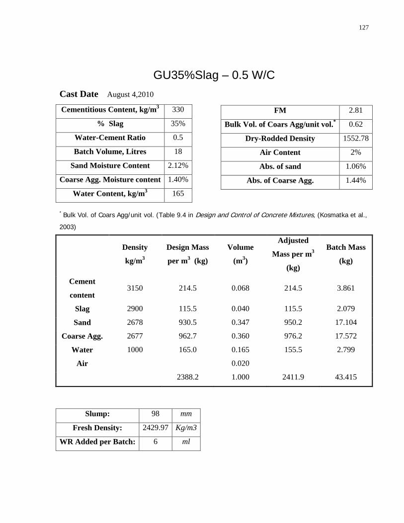
127
GU35%Slag – 0.5 W/C Cast Date August 4,2010
Cementitious Content, kg/m3 330
% Slag 35%
Water-Cement Ratio 0.5
Batch Volume, Litres 18
Sand Moisture Content 2.12%
Coarse Agg. Moisture content 1.40%
Water Content, kg/m3 165
* Bulk Vol. of Coars Agg/unit vol. (Table 9.4 in Design and Control of Concrete Mixtures, (Kosmatka et al.,
2003)
Density
kg/m3
Design Mass
per m3 (kg)
Volume
(m3)
Adjusted
Mass per m3
(kg)
Batch Mass
(kg)
Cement
content 3150 214.5 0.068 214.5 3.861
Slag 2900 115.5 0.040 115.5 2.079
Sand 2678 930.5 0.347 950.2 17.104
Coarse Agg. 2677 962.7 0.360 976.2 17.572
Water 1000 165.0 0.165 155.5 2.799
Air 0.020
2388.2 1.000 2411.9 43.415
Slump: 98 mm
Fresh Density: 2429.97 Kg/m3
WR Added per Batch: 6 ml
FM 2.81
Bulk Vol. of Coars Agg/unit vol.* 0.62
Dry-Rodded Density 1552.78
Air Content 2%
Abs. of sand 1.06%
Abs. of Coarse Agg. 1.44%

128
GU35%Slag – 0.5 W/C
Mix ID: T5 - Trial Mix #5 ( specimens from this mix were used in the NT Build 49 with the modified test lengths.
Cast Date July 29, 2010
Cementitious Content, kg/m3 330
% Slag 35%
Water-Cement Ratio 0.5
Batch Volume, Litres 18
Sand Moisture Content 2.12%
Coarse Agg. Moisture content 1.40%
Water Content, kg/m3 165
* Bulk Vol. of Coars Agg/unit vol. (Table 9.4 in Design and Control of Concrete Mixtures, (Kosmatka et al.,
2003)
Density
kg/m3
Design Mass
per m3 (kg)
Volume
(m3)
Adjusted
Mass per m3
(kg)
Batch Mass
(kg)
Cement
content 3150 214.5 0.068 214.5 3.861
Slag 2900 115.5 0.040 115.5 2.079 Sand 2678 930.5 0.347 950.2 17.104
Coarse Agg. 2677 962.7 0.360 976.2 17.572 Water 1000 165.0 0.165 155.5 2.799
Air 0.020 2388.2 1.000 2411.9 43.415
Slump: 80 mm
Fresh Density: - Kg/m3
WR Added per Batch: 6 ml
FM 2.81
Bulk Vol. of Coars Agg/unit vol.* 0.62
Dry-Rodded Density 1552.78
Air Content 2%
Abs. of sand 1.06%
Abs. of Coarse Agg. 1.44%

129
100%GU – 0.5 W/C
Mix ID: 0.5/GU Cast Date August 11,2010
Cementitious Content, kg/m3 330
% Slag 0%
Water-Cement Ratio 0.5
Batch Volume, Litres 18
Sand Moisture Content 2.18%
Coarse Agg. Moisture content 0.39%
Water Content, kg/m3 165
* Bulk Vol. of Coars Agg/unit vol. (Table 9.4 in Design and Control of Concrete Mixtures, (Kosmatka et al.,
2003)
Density
kg/m3
Design Mass
per m3 (kg)
Volume
(m3)
Adjusted
Mass per m3
(kg)
Batch Mass
(kg)
Cement
content 3150 330.0 0.105 330.0 5.940
Slag 2900 0.0 0.000 0.0 0.000
Sand 2678 938.9 0.351 959.4 17.269
Coarse Agg. 2677 962.7 0.360 966.5 17.397
Water 1000 165.0 0.165 164.6 2.963
Air 0.020
2396.7 1.000 2420.5 43.569
Slump: 74 mm
Fresh Density: 2418.77 Kg/m3
WR Added per Batch: 6 ml
FM 2.81
Bulk Vol. of Coars Agg/unit vol.* 0.62
Dry-Rodded Density 1552.78
Air Content 2%
Abs. of sand 1.06%
Abs. of Coarse Agg. 1.44%
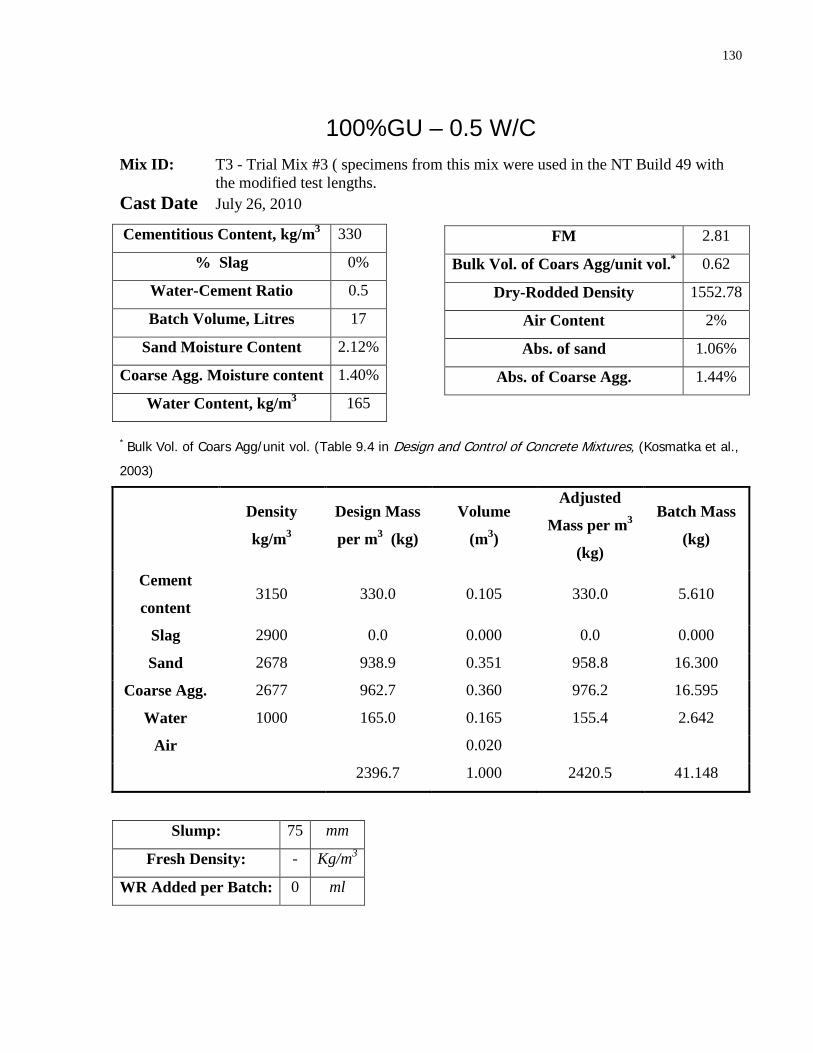
130
100%GU – 0.5 W/C
Mix ID: T3 - Trial Mix #3 ( specimens from this mix were used in the NT Build 49 with the modified test lengths.
Cast Date July 26, 2010
Cementitious Content, kg/m3 330
% Slag 0%
Water-Cement Ratio 0.5
Batch Volume, Litres 17
Sand Moisture Content 2.12%
Coarse Agg. Moisture content 1.40%
Water Content, kg/m3 165
* Bulk Vol. of Coars Agg/unit vol. (Table 9.4 in Design and Control of Concrete Mixtures, (Kosmatka et al.,
2003)
Density
kg/m3
Design Mass
per m3 (kg)
Volume
(m3)
Adjusted
Mass per m3
(kg)
Batch Mass
(kg)
Cement
content 3150 330.0 0.105 330.0 5.610
Slag 2900 0.0 0.000 0.0 0.000
Sand 2678 938.9 0.351 958.8 16.300
Coarse Agg. 2677 962.7 0.360 976.2 16.595
Water 1000 165.0 0.165 155.4 2.642
Air 0.020
2396.7 1.000 2420.5 41.148
Slump: 75 mm
Fresh Density: - Kg/m3
WR Added per Batch: 0 ml
FM 2.81
Bulk Vol. of Coars Agg/unit vol.* 0.62
Dry-Rodded Density 1552.78
Air Content 2%
Abs. of sand 1.06%
Abs. of Coarse Agg. 1.44%

131
GU50%Slag – 0.45 W/C
Cast Date August 18,2010
Cementitious Content, kg/m3 366.7
% Slag 0%
Water-Cement Ratio 0.45
Batch Volume, Litres 18
Sand Moisture Content 2.18%
Coarse Agg. Moisture content 0.19%
Water Content, kg/m3 165
* Bulk Vol. of Coars Agg/unit vol. (Table 9.4 in Design and Control of Concrete Mixtures, (Kosmatka et al.,
2003)
Density
kg/m3
Design Mass
per m3 (kg)
Volume
(m3)
Adjusted
Mass per m3
(kg)
Batch Mass
(kg)
Cement
content 3150 183.3 0.058 183.3 3.300
Slag 2900 183.3 0.063 183.3 3.300
Sand 2678 894.3 0.334 913.8 16.449
Coarse Agg. 2677 962.7 0.360 964.6 17.362
Water 1000 165.0 0.165 167.0 3.006
Air 0.020
2388.7 1.000 2412.1 43.417
Slump: 62 mm
Fresh Density: 24118.06 Kg/m3
WR Added per Batch: 6.5 ml
FM 2.81
Bulk Vol. of Coars Agg/unit vol.* 0.62
Dry-Rodded Density 1552.78
Air Content 2%
Abs. of sand 1.06%
Abs. of Coarse Agg. 1.44%

132
GU50%Slag – 0.4 W/C Cast Date August 24,2010
Cementitious Content, kg/m3 412.5
% Slag 50%
Water-Cement Ratio 0.4
Batch Volume, Litres 18
Sand Moisture Content 4.68%
Coarse Agg. Moisture content 1.01%
Water Content, kg/m3 165
* Bulk Vol. of Coars Agg/unit vol. (Table 9.4 in Design and Control of Concrete Mixtures, (Kosmatka et al.,
2003)
Density
kg/m3
Design Mass
per m3 (kg)
Volume
(m3)
Adjusted
Mass per m3
(kg)
Batch Mass
(kg)
Cement
content 3150 206.3 0.065 206.3 3.713
Slag 2900 206.3 0.071 206.3 3.713
Sand 2678 853.7 0.319 893.6 16.085
Coarse Agg. 2677 962.7 0.360 972.4 17.504
Water 1000 165.0 0.165 138.2 2.488
Air 0.020
2393.9 1.000 2416.8 43.503
Slump: 110 mm
Fresh Density: 2433.47 Kg/m3
WR Added per Batch: 15 ml
FM 2.81
Bulk Vol. of Coars Agg/unit vol.* 0.62
Dry-Rodded Density 1552.78
Air Content 2%
Abs. of sand 1.06%
Abs. of Coarse Agg. 1.44%

133
100% InterCem (GUb-30F) – 0.5 W/C Cast Date August 26,2010
Cementitious Content, kg/m3 330
% Slag 0%
Water-Cement Ratio 0.5
Batch Volume, Litres 18
Sand Moisture Content 4.68%
Coarse Agg. Moisture content 1.01%
Water Content, kg/m3 165
* Bulk Vol. of Coars Agg/unit vol. (Table 9.4 in Design and Control of Concrete Mixtures, (Kosmatka et al.,
2003)
Density
kg/m3
Design Mass
per m3 (kg)
Volume
(m3)
Adjusted
Mass per m3
(kg)
Batch Mass
(kg)
Cement
content 3150 330.0 0.105 330.0 5.940
Slag 2900 0.0 0.000 0.0 0.000
Sand 2678 938.9 0.351 982.9 17.692
Coarse Agg. 2677 962.7 0.360 972.4 17.504
Water 1000 165.0 0.165 135.2 2.433
Air 0.020
2396.7 1.000 2420.5 43.569
Slump: 115 mm
Fresh Density: 2424.37 Kg/m3
WR Added per Batch: 6 ml
FM 2.81
Bulk Vol. of Coars Agg/unit vol.* 0.62
Dry-Rodded Density 1552.78
Air Content 2%
Abs. of sand 1.06%
Abs. of Coarse Agg. 1.44%

134
100%HS – 0.45 W/C Cast Date September 22, 2010
Cementitious Content, kg/m3 366.7
% Slag 0%
Water-Cement Ratio 0.45
Batch Volume, Litres 18
Sand Moisture Content 3.72%
Coarse Agg. Moisture content 0.93%
Water Content, kg/m3 165
* Bulk Vol. of Coars Agg/unit vol. (Table 9.4 in Design and Control of Concrete Mixtures, (Kosmatka et al.,
2003)
Density
kg/m3
Design Mass
per m3 (kg)
Volume
(m))
Adjusted
Mass per m3
(kg)
Batch Mass
(kg)
Cement
content 3150 366.7 0.116 366.7 6.600
Slag 2900 0.0 0.000 0.0 0.000
Sand 2678 907.8 0.339 941.5 16.948
Coarse Agg. 2677 962.7 0.360 971.7 17.490
Water 1000 165.0 0.165 145.8 2.624
Air 0.020
2402.2 1.000 2425.6 43.661
Slump: 118 mm
Fresh Density: 2400.56 Kg/m3
WR Added per Batch: 7 ml
FM 2.81
Bulk Vol. of Coars Agg/unit vol.* 0.62
Dry-Rodded Density 1552.78
Air Content 2%
Abs. of sand 1.06%
Abs. of Coarse Agg. 1.44%

135
100%HS – 0.4 W/C Cast Date October 5, 2010
Cementitious Content, kg/m3 412.5
% Slag 0%
Water-Cement Ratio 0.4
Batch Volume, Litres 18
Sand Moisture Content 3.84%
Coarse Agg. Moisture content 0.91%
Water Content, kg/m3 165
* Bulk Vol. of Coars Agg/unit vol. (Table 9.4 in Design and Control of Concrete Mixtures, (Kosmatka et al.,
2003)
Density
kg/m3
Design Mass
per m3 (kg)
Volume
(m))
Adjusted
Mass per m3
(kg)
Batch Mass
(kg)
Cement
content 3150 412.5 0.131 412.5 7.425
Slag 2900 0.0 0.000 0.0 0.000
Sand 2678 868.8 0.324 902.2 16.239
Coarse Agg. 2677 962.7 0.360 971.5 17.487
Water 1000 165.0 0.165 145.9 2.627
Air 0.020
2409.0 1.000 2432.1 43.778
Slump: 90 mm
Fresh Density: 2448.88 Kg/m3
WR Added per Batch: 7 ml
FM 2.81
Bulk Vol. of Coars Agg/unit vol.* 0.62
Dry-Rodded Density 1552.78
Air Content 2%
Abs. of sand 1.06%
Abs. of Coarse Agg. 1.44%

136
100%MS – 0.5 W/C
Cast Date October 7, 2010
Cementitious Content, kg/m3 330
% Slag 0%
Water-Cement Ratio 0.5
Batch Volume, Litres 18
Sand Moisture Content 3.84%
Coarse Agg. Moisture content 0.91%
Water Content, kg/m3 165
* Bulk Vol. of Coars Agg/unit vol. (Table 9.4 in Design and Control of Concrete Mixtures, (Kosmatka et al.,
2003)
Density
kg/m3
Design Mass
per m3 (kg)
Volume
(m))
Adjusted
Mass per m3
(kg)
Batch Mass
(kg)
Cement
content 3150 330.0 0.105 330.0 5.940
Slag 2900 0.0 0.000 0.0 0.000
Sand 2678 938.9 0.351 975.0 17.550
Coarse Agg. 2677 962.7 0.360 971.5 17.487
Water 1000 165.0 0.165 144.0 2.592
Air 0.020
2396.7 1.000 2420.5 43.569
Slump: 100 mm
Fresh Density: 2430.67 Kg/m3
WR Added per Batch: 6 ml
FM 2.81
Bulk Vol. of Coars Agg/unit vol.* 0.62
Dry-Rodded Density 1552.78
Air Content 2%
Abs. of sand 1.06%
Abs. of Coarse Agg. 1.44%
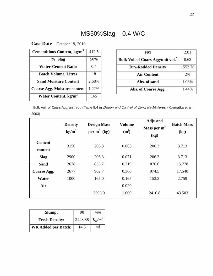
137
MS50%Slag – 0.4 W/C
Cast Date October 19, 2010
Cementitious Content, kg/m3 412.5
% Slag 50%
Water-Cement Ratio 0.4
Batch Volume, Litres 18
Sand Moisture Content 2.68%
Coarse Agg. Moisture content 1.22%
Water Content, kg/m3 165
* Bulk Vol. of Coars Agg/unit vol. (Table 9.4 in Design and Control of Concrete Mixtures, (Kosmatka et al.,
2003)
Density
kg/m3
Design Mass
per m3 (kg)
Volume
(m))
Adjusted
Mass per m3
(kg)
Batch Mass
(kg)
Cement
content 3150 206.3 0.065 206.3 3.713
Slag 2900 206.3 0.071 206.3 3.713
Sand 2678 853.7 0.319 876.6 15.778
Coarse Agg. 2677 962.7 0.360 974.5 17.540
Water 1000 165.0 0.165 153.3 2.759
Air 0.020
2393.9 1.000 2416.8 43.503
Slump: 98 mm
Fresh Density: 2448.88 Kg/m3
WR Added per Batch: 14.5 ml
FM 2.81
Bulk Vol. of Coars Agg/unit vol.* 0.62
Dry-Rodded Density 1552.78
Air Content 2%
Abs. of sand 1.06%
Abs. of Coarse Agg. 1.44%

138
Appendix C ASTM C 1202 Data

139
Calculations:
6 Hours Data
𝐴𝑑𝑗𝑢𝑠𝑡𝑒𝑑 𝐶ℎ𝑎𝑟𝑔𝑒(𝐶𝑜𝑢𝑙𝑜𝑚𝑏𝑠) = 𝐴𝑐𝑡𝑢𝑎𝑙 𝐶ℎ𝑎𝑟𝑔𝑒(𝐶𝑜𝑢𝑙𝑜𝑚𝑏𝑠) × �95𝑚𝑚𝐷 𝑚𝑚
�2
𝐴𝑣𝑒𝑟𝑎𝑔𝑒 6ℎ𝑟𝑠 𝐶𝑢𝑟𝑟𝑒𝑛𝑡 (𝑚𝐴) = �𝐴𝑐𝑡𝑢𝑎𝑙 𝐶ℎ𝑎𝑟𝑔𝑒 ( 𝐶𝑜𝑢𝑙𝑜𝑚𝑏𝑠)𝑇𝑒𝑠𝑡 𝐷𝑢𝑟𝑎𝑡𝑖𝑜𝑛 (𝑠)
� × 1000
𝐴𝑣𝑒𝑟𝑎𝑔𝑒 6ℎ𝑟𝑠 𝑅𝑒𝑠𝑖𝑠𝑡𝑎𝑛𝑐𝑒,𝑅, (𝑜ℎ𝑚𝑠) = 60 𝑉𝑜𝑙𝑡𝑠
𝐴𝑣𝑒𝑟𝑎𝑔𝑒 6ℎ𝑟𝑠 𝐶𝑢𝑟𝑟𝑒𝑛𝑡 (𝐴𝑚𝑝𝑠)
𝐴𝑣𝑒𝑟𝑎𝑔𝑒 6 ℎ𝑟𝑠 𝑅𝑒𝑠𝑖𝑠𝑡𝑖𝑣𝑖𝑡𝑦,𝜌, (𝑜ℎ𝑚𝑠 ∙ 𝑚)
= 𝐴𝑣𝑒𝑟𝑎𝑔𝑒 6ℎ𝑟𝑠 𝑅𝑒𝑠𝑖𝑠𝑡𝑎𝑛𝑐𝑒(𝑜ℎ𝑚𝑠) × 𝐶𝑟𝑜𝑠𝑠 − 𝑆𝑒𝑐𝑡𝑖𝑜𝑛𝑎𝑙 𝐴𝑟𝑒𝑎 𝑜𝑓 𝑆𝑎𝑚𝑝𝑙𝑒 (𝑚2)
𝐿𝑒𝑛𝑔𝑡ℎ 𝑜𝑓 𝑆𝑎𝑚𝑝𝑙𝑒 (𝑚)
1 and 5 minutes Data
𝐼𝑛𝑠𝑡𝑎𝑛𝑡𝑎𝑛𝑒𝑜𝑢𝑠 𝑅𝑒𝑠𝑖𝑠𝑡𝑎𝑛𝑐𝑒,𝑅, (𝑜ℎ𝑚𝑠) = 60 𝑉𝑜𝑙𝑡𝑠
𝐼𝑛𝑠𝑡𝑎𝑛𝑡𝑎𝑛𝑒𝑜𝑢𝑠 𝐶𝑢𝑟𝑟𝑒𝑛𝑡 (𝐴𝑚𝑝𝑠)
𝐼𝑛𝑠𝑡𝑎𝑛𝑡𝑎𝑛𝑒𝑜𝑢𝑠 𝑅𝑒𝑠𝑖𝑠𝑡𝑖𝑣𝑖𝑡𝑦,𝜌, (𝑜ℎ𝑚𝑠 ∙ 𝑚)
=𝐼𝑛𝑠𝑡𝑎𝑛𝑡𝑎𝑛𝑒𝑜𝑢𝑠 𝑅𝑒𝑠𝑖𝑠𝑡𝑎𝑛𝑐𝑒(𝑜ℎ𝑚𝑠) × 𝐶𝑟𝑜𝑠𝑠 − 𝑆𝑒𝑐𝑡𝑖𝑜𝑛𝑎𝑙 𝐴𝑟𝑒𝑎 𝑜𝑓 𝑆𝑎𝑚𝑝𝑙𝑒 (𝑚2)
𝐿𝑒𝑛𝑔𝑡ℎ 𝑜𝑓 𝑆𝑎𝑚𝑝𝑙𝑒 (𝑚)

140
Mix: 0.5/GU/35S
Age: 35 Days
Sample Data
Exposure Solution
Chloride Sulphate
Sample ID
1A 2B 1B 2A
D (mm) 102.11 101.58 101.66 102.23
L (mm) 51.37 51.65 51.41 51.74
A (m2) 0.0081889 0.008104128 0.008117 0.008208
6 Hours Data
Actual Charge
passed (Coulombs) 1140 1144 1084 990
Adjusted Charge
(Coulombs) 986.76903 1000.59152 946.6213 854.9204
Avg 6hr Current
(mA) 52.777778 52.96296296 50.18519 45.83333
Avg 6hr R (ohms) 1136.8421 1132.867133 1195.572 1309.091
Avg 6hr ρ
(ohms *m) 181.22455 177.7521857 188.7636 207.6778
1 Minute Data
Current (mA) 23.5 24 57.6 58.9
Instant. R (ohms) 2553.191489 2500 1041.667 1018.676
Instant. ρ
(ohms*m) 407.0054795 394.714 165.2528 159.835
5 Minute Data
Current (mA) 34.7 58.7 56.5 56.6
Instant. R (ohms) 1729.107 1022.147 1061.947 1060.071
Instant. ρ
(ohms*m) 275.6377 160.3796 167.6661 168.1725

141
Mix: 0.5/GU/35S
Age: 56 Days
Sample Data
Exposure Solution
Chloride Sulphate
Sample ID
1A 2B 1B 2A
D (mm) 102.26 101.83 101.95 102.14
L (mm) 50.76 50.92 50.6 50.44
A (m2) 0.008212993 0.008144068 0.008163273 0.008193729
6 Hours Data
Actual Charge
passed (Coulombs) 1005 1019 796 926
Adjusted Charge
(Coulombs) 867.3646047 886.8903042 691.1714938 801.0626634
Avg 6hr Current
(mA) 46.52777778 47.17592593 36.85185185 42.87037037
Avg 6hr R (ohms) 1289.552239 1271.835132 1628.140704 1399.568035
Avg 6hr ρ
(ohms *m) 208.65019 203.4153824 262.667148 227.3529142
1 Minute Data
Current (mA) 48.5 48 43 48.6
Instant. R (ohms) 1237.113 1250 1395.349 1234.568
Instant. ρ
(ohms*m) 200.1656 199.9231 225.1109 200.5495
5 Minute Data
Current (mA) 48 48 43.6 48.2
Instant. R (ohms) 1250 1250 1376.147 1244.813
Instant. ρ
(ohms*m) 202.2506 199.9231 222.0131 202.2138

142
Mix: 0.5/GU
Age: 35 Days
Sample Data
Exposure Solution
Chloride Sulphate
Sample ID
1A 2B 1B 2A
D (mm) 102.095 101.97 101.71 102.38
L (mm) 49.28 48.99 49.44 49.5
A (m2) 0.0081865 0.008166477 0.008125 0.008232
6 Hours Data
Actual Charge
passed (Coulombs) 2894 2773 2225 2321
Adjusted Charge
(Coulombs) 2505.7445 2406.867826 1941.109 1998.445
Avg 6hr Current
(mA) 133.98148 128.3796296 103.0093 107.4537
Avg 6 hr R (ohms) 447.82308 467.3638658 582.4719 558.38
Avg 6hr ρ
(ohms *m) 74.393434 77.90806402 95.72243 92.86345
1 Minute Data
Current (mA) 130.8 121.8 130.5 130.4
Instant. R (ohms) 458.7155963 492.6108 459.7701 460.1227
Instant. ρ
(ohms*m) 76.20292391 82.11665 75.55783 76.5224
5 Minute Data
Current (mA) 129.5 122.1 128.4 129
R (ohms) 463.3205 491.4005 467.2897 465.1163
Instant. ρ
(ohms*m) 76.9679 81.91489 76.79359 77.35288

143
Mix: 0.5/GU
Age: 56 Days
Sample Data
Exposure Solution
Chloride Sulphate
Sample ID
1A 2B 1B 2A
D (mm) 102.11 101.86 101.73 102.29
L (mm) 48.6 50.81 50.69 50.61
A (m2) 0.008188916 0.008148867 0.00812808 0.008217813
6 Hours Data
Actual Charge
passed (Coulombs) 2611 2471 1752 1901
Adjusted Charge
(Coulombs) 2260.047308 2149.377074 1527.858812 1639.694614
Avg 6 hr Current
(mA) 120.8796296 114.3981481 81.11111111 88.00925926
Avg 6 hr R (ohms) 496.3615473 524.4840146 739.7260274 681.7464492
Avg 6 hr ρ
(ohms *m) 83.63504486 84.11632422 118.6141713 110.6987676
1 Minute Data
Current (mA) 130.8 121.8 130.5 130.4
Instant. R (ohms) 458.7155963 492.6108 459.7701 460.1227
Instant. ρ
(ohms*m) 76.20292391 82.11665 75.55783 76.5224
5 Minute Data
Current (mA) 129.5 122.1 128.4 129
Instant. R (ohms) 463.3205 491.4005 467.2897 465.1163
Instant. ρ
(ohms*m) 76.9679 81.91489 76.79359 77.35288

144
Mix: 0.45/GU/50S
Age: 35 Days
Sample Data
Exposure Solution
Chloride Sulphate
Sample ID
1A 2B 1B 2A
D (mm) 101.72 101.59 101.83 102.39
L (mm) 50.1 50.32 49.92 49.42
A (m2) 0.0081265 0.008105724 0.008144 0.008234
6 Hours Data
Actual Charge
passed (Coulombs) 813 849 671 838
Adjusted Charge
(Coulombs) 709.12868 742.425671 584.0073 721.4
Avg 6hr Current
(mA) 37.638889 39.30555556 31.06481 38.7963
Avg 6hr R (ohms) 1594.0959 1526.501767 1931.446 1546.539
Avg 6hr ρ
(ohms *m) 258.5707 245.8943109 315.1006 257.6696
1 Minute Data
Current (mA) 41.5 40.7 30.1 46.2
Instant. R (ohms) 1445.783133 1474.201 1993.355 1298.701
Instant. ρ
(ohms*m) 234.5135885 237.4696 325.2008 216.3772
5 Minute Data
Current (mA) 40.8 40.4 36 45.3
Instant. R (ohms) 1470.588 1485.149 1666.667 1324.503
Instant. ρ
(ohms*m) 238.5371 239.233 271.904 220.6761

145
Mix: 0.45/GU/50S
Age: 56 Days
Sample Data
Exposure Solution
Chloride Sulphate
Sample ID
1A 2B 1B 2A
D (mm) 102.06 101.71 101.66 102.2
L (mm) 49.95 50.45 50.43 50.59
A (m2) 0.008180899 0.008124884 0.008116898 0.008203358
6 Hours Data
Actual Charge
passed (Coulombs) 680 520 648 656
Adjusted Charge
(Coulombs) 589.175929 454.0987888 559.9128373 572.299994
Avg 6hr Current
(mA) 31.48148148 24.07407407 30 30.37037037
Avg 6hr R (ohms) 1905.882353 2492.307692 2000 1975.609756
Avg 6hr ρ
(ohms *m) 312.1487539 401.1462917 324.3074976 318.1685008
1 Minute Data
Current (mA) 31.5 30.2 26.8 32
Instant. R (ohms) 1904.762 1986.755 2238.806 1875
Instant. ρ
(ohms*m) 311.9652 319.9634 360.3442 304.0383
5 Minute Data
Current (mA) 31.3 30.3 24.9 31.8
Instant. R (ohms) 1916.933 1980.198 2409.639 1886.792
Instant. ρ
(ohms*m) 313.9586 318.9074 387.8404 305.9505

146
Mix: 0.4/GU/50S
Age: 35 Days
Sample Data
Exposure Solution
Chloride Sulphate
Sample ID
1A 2B 1B 2A
D (mm) 102.09 101.77 102.2 101.95
L (mm) 49.12 50.48 50.7 50.44
A (m2) 0.0081857 0.008134 0.008203 0.008163273
6 Hours Data
Actual Charge
passed (Coulombs) 928 639 786 881
Adjusted Charge
(Coulombs) 803.57937 556.8119 679.1535 764.977495
Avg 6hr Current
(mA) 42.962963 29.58333 36.38889 40.78703704
Avg 6hr R (ohms) 1396.5517 2028.169 1648.855 1471.055619
Avg 6 hr ρ
(ohms *m) 232.73139 326.8242 266.7879 238.0775018
1 Minute Data
Current (mA) 45.3 43 33.7 40.9
Instant. R (ohms) 1324.503311 1395.349 1780.415 1466.993
Instant. ρ
(ohms*m) 220.7247224 225.825 286.9006 237.3623
5 Minute Data
Current (mA) 44.9 42.8 33.8 40.3
Instant. R (ohms) 1336.303 1401.869 1775.148 1488.834
Instant. ρ
(ohms*m) 222.6911 226.8803 286.0518 240.8962

147
Mix: 0.4/GU/50S
Age: 56 Days
Sample Data
Exposure Solution
Chloride Sulphate
Sample ID
1A 2B 1B 2A
D (mm) 102.02 101.66 102.1 101.8
L (mm) 49.18 49.11 48.61 48.97
A (m2) 0.008174487 0.008116898 0.008187312 0.00813927
6 Hours Data
Actual Charge
passed (Coulombs) 753 702 665 709
Adjusted Charge
(Coulombs) 652.9374043 611.3483814 580.7224895 613.8213098
Avg 6hr Current
(mA) 34.86111111 32.5 30.78703704 32.82407407
Avg hr R (ohms) 1721.115538 1846.153846 1948.87218 1827.926657
Avg 6r ρ
(ohms *m) 286.0763926 306.8479476 322.1094855 307.8750609
1 Minute Data
Current (mA) 37.1 35.6 36.6 37.5
Instant. R (ohms) 1617.251 1685.393 1639.344 1600
Instant. ρ
(ohms*m) 268.8124 280.128 270.9507 269.4857
5 Minute Data
Current (mA) 36.1 35.4 36.3 36.9
Instant. R (ohms) 1662.05 1694.915 1652.893 1626.016
Instant. ρ
(ohms*m) 276.2588 281.7107 273.19 273.8676

148
Mix: 0.5/InterCem
Age: 35 Days
Sample Data
Exposure Solution
Chloride Sulphate
Sample ID
1A 2B 1B 2A
D (mm) 101.53 101.8 101.45 102.31
L (mm) 50.49 50.81 50.65 50.43
A (m2) 0.0080962 0.00813927 0.008083 0.008221
6 Hours Data
Actual Charge
passed (Coulombs) 1142 1091 993 1041
Adjusted Charge
(Coulombs) 999.82627 950.1155044 870.7477 897.5564
Avg 6hr Current
(mA) 52.87037 50.50925926 45.97222 48.19444
Avg 6hr R (ohms) 1134.8511 1187.901008 1305.136 1244.957
Avg 6hr ρ
(ohms *m) 181.97519 190.290231 208.2909 202.9511
1 Minute Data
Current (mA) 53 49.8 46.3 52.2
Instant. R (ohms) 1132.075472 1204.819 1295.896 1149.425
Instant. ρ
(ohms*m) 181.5301071 193.0004 206.8163 187.3777
5 Minute Data
Current (mA) 52.3 40 45.5 51.6
Instant. R (ohms) 1147.228 1500 1318.681 1162.791
Instant.ρ (ohms*m) 183.9598 240.2855 210.4526 189.5565

149
Mix: 0.5/InterCem
Age: 56 Days
Sample Data
Exposure Solution
Chloride Sulphate
Sample ID
1A 2B 1B 2A
D (mm) 102.23 101.7 101.78 101.99
L (mm) 49 49.18 49.22 48.79
A (m2) 0.008208175 0.008123287 0.008136072 0.00816968
6 Hours Data
Actual Charge
passed (Coulombs) 686 621 591 712.41
Actual Adjusted
Charge (Coulombs) 592.3993928 541.0207445 512.7663391 621.6347897
Avg 6hr Current
(mA) 31.75925926 28.75 27.36111111 32.98194444
Avg 6hr R (ohms) 1889.212828 2086.956522 2192.893401 1819.177159
Avg 6hr ρ
(ohms *m) 316.4691705 344.9741605 367.1907798 300.4818589
1 Minute Data
Current (mA) 31.6 33.3 31.2 31.6
Instant. R (ohms) 1898.734 1801.802 1923.077 1898.734
Instant. ρ
(ohms*m) 318.0641 297.6119 317.8848 317.9351
5 Minute Data
Current (mA) 31.2 33 31.1 30.9
Instant. R (ohms) 1923.077 1818.182 1929.26 1941.748
Instant. ρ
(ohms*m) 322.1419 300.3175 318.907 325.1375

150
Mix: 0.45/HS
Age: 35 Days
Sample Data
Exposure Solution
Chloride Sulphate
Sample ID
1A 2B 1B 2A
D (mm) 101.83 101.77 101.77 102.01
L (mm) 50.57 50.05 50.55 50.76
A (m2) 0.0081441 0.008134473 0.008134 0.008173
6 Hours Data
Actual Charge
passed (Coulombs) 3971 3745 2710 2488
Adjusted Charge
(Coulombs) 3456.1741 3263.318655 2361.44 2157.804
Avg 6hr Current
(mA) 183.84259 173.3796296 125.463 115.1852
Avg 6hr R (ohms) 326.36615 346.0614152 478.2288 520.9003
Avg 6hr ρ
(ohms *m) 52.559779 56.24430156 76.95626 83.87034
1 Minute Data
Current (mA) 157.2 150.8 143.5 144.2
Instant. R (ohms) 381.6793893 397.878 418.1185 416.0888
Instant. ρ
(ohms*m) 61.46772278 64.66589 67.28335 66.99459
5 Minute Data
Current (mA) 154.5 150.3 138.9 140
Instant. R (ohms) 388.3495 399.2016 431.9654 428.5714
Instant. ρ
(ohms*m) 62.54192 64.88101 69.5116 69.00443

151
Mix: 0.45/HS
Age: 56 Days
Sample Data
Exposure Solution
Chloride Sulphate
Sample ID
1A 2B 1B 2A
D (mm) 101.935 101.74 101.62 101.95
L (mm) 49.68 50.03 50.4 50.19
A (m2) 0.008160871 0.008129678 0.008110512 0.008163273
6 Hours Data
Actual Charge
passed (Coulombs) 3176 3784 2225 2829
Adjusted Charge
(Coulombs) 2758.551205 3299.247313 1944.548792 2456.437382
Avg 6hr Current
(mA) 147.037037 175.1851852 103.0092593 130.9722222
Avg 6hr R (ohms) 408.0604534 342.4947146 582.4719101 458.1124072
Avg 6hr ρ
(ohms *m) 67.03158003 55.65404295 93.73304211 74.51079548
1 Minute Data
Current (mA) 134.5 148.8 115.7 153.8
Instant. R (ohms) 446.0967 403.2258 518.5825 390.117
Instant. ρ
(ohms*m) 73.27974 65.52261 83.45178 63.45152
5 Minute Data
Current (mA) 132.1 148 114.9 148.1
Instant. R (ohms) 454.2014 405.4054 522.1932 405.1317
Instant. ρ
(ohms*m) 74.61109 65.87678 84.03282 65.89362

152
Mix: 0.4/HS
Age: 35 Days
Sample Data
Exposure Solution
Chloride Sulphate
Sample ID
1A 2B 1B 2A
D (mm) 102 101.54 101.61 101.82
L (mm) 52.31 51.28 52.39 53.1
A (m2) 0.0081713 0.008097747 0.008109 0.008142
6 Hours Data
Actual Charge
passed (Coulombs) 3619 3580 2625 2938
Adjusted Charge
(Coulombs) 3139.319 3133.689187 2294.582 2557.601
Avg 6hrs Current
(mA) 167.5463 165.7407407 121.5278 136.0185
Avg 6hr R (ohms) 358.10998 362.0111732 493.7143 441.1164
Avg 6hr ρ
(ohms *m) 55.939931 57.16604645 76.41702 67.64174
1 Minute Data
Current (mA) 143.6 147.4 137.1 140.3
Instant. R (ohms) 417.8272981 407.0556 437.6368 427.655
Instant. ρ
(ohms*m) 65.26830215 64.27912 67.73735 65.57754
5 Minute Data
Current (mA) 135.6 139.7 132.6 132.3
Instant. R (ohms) 442.4779 429.4918 452.4887 453.5147
Instant. ρ
(ohms*m) 69.11894 67.82207 70.03613 69.54292

153
Mix: 0.4/HS
Age: 56 Days
Sample Data
Exposure Solution
Chloride Sulphate
Sample ID
1A 2B 1B 2A
D (mm) 102.14 102.07 101.58 102.16
L (mm) 49.81 48.86 49.92 50
A (m2) 0.008193729 0.008182502 0.008104128 0.008196938
6 Hours Data
Actual Charge
passed (Coulombs) 2986 3205 2194 2190
Adjusted Charge
(Coulombs) 2583.124312 2776.380688 1918.966604 1893.780136
Avg 6hr Current
(mA) 138.2407407 148.3796296 101.5740741 101.3888889
Avg 6hr R (ohms) 434.0254521 404.3681747 590.7019143 591.7808219
Avg 6hr ρ
(ohms *m) 71.39704621 67.71885649 95.89591337 97.01581407
1 Minute Data
Current (mA) 124.9 128.7 114.2 125.5
Instant. R (ohms) 480.3843 466.2005 525.394 478.0876
Instant. ρ
(ohms*m) 79.02306 78.07381 85.29368 78.3771
5 Minute Data
Current (mA) 123.6 128.8 112.8 120.4
Instant. R (ohms) 485.4369 465.8385 531.9149 498.3389
Instant. ρ
(ohms*m) 79.85421 78.01319 86.35229 81.69706

154
Mix: 0.5/MS
Age: 35 Days
Sample Data
Exposure Solution
Chloride Sulphate
Sample ID
1A 2B 1B 2A
D (mm) 101.96 101.73 101.51 102.13
L (mm) 50.97 51.06 50.61 50.95
A (m2) 0.0081649 0.00812808 0.008093 0.008192
6 Hours Data
Actual Charge
passed (Coulombs) 3446 3858 2537 2450
Adjusted Charge
(Coulombs) 2991.595 3364.429 2222.031 2119.857
Avg 6hr Current
(mA) 159.537 178.611 117.454 113.426
Avg 6hr R (ohms) 376.088 335.925 510.840 528.980
Avg 6hr ρ
(ohms *m) 60.246 53.475 81.688 85.053
1 Minute Data
Current (mA) 139.8 149.8 135 145.7
Instant. R (ohms) 429.1845494 400.534 444.444 411.805
Instant. ρ
(ohms*m) 68.751 63.760 71.070 66.213
5 Minute Data
Current (mA) 12 147.1 131.1 140.2
Instant. R (ohms) 446.429 407.886 457.666 427.960
Instant. ρ
(ohms*m) 71.513 64.930 73.185 68.811

155
Mix: 0.5/MS
Age: 56 Days
Sample Data
Exposure Solution
Chloride Sulphate
Sample ID
1A 2B 1B 2A
D (mm) 102.17 101.88 102.17 101.72
L (mm) 49.95 49.8 49.98 49.65
A (m2) 0.008198543 0.008152067 0.008198543 0.008126482
6 Hours Data
Actual Charge
passed (Coulombs) 3555 3382 2462 2380
Adjusted Charge
(Coulombs) 3073.548 2949.906 2140.708 2057.678
Avg 6hr Current
(mA) 164.583 156.574 113.981 110.185
Avg 6hr R (ohms) 364.557 383.205 526.401 544.538
Avg 6hr ρ
(ohms *m) 59.837 62.721 86.170 89.324
1 Minute Data
Current (mA) 145.6 138.1 132.3 139.7
Instant. R (ohms) 412.088 434.468 453.515 429.492
Instant. ρ
(ohms*m) 67.638 71.112 74.239 70.452
5 Minute Data
Current (mA) 144.8 138.4 131.6 143.6
Instant. R (ohms) 414.365 433.526 455.927 417.827
Instant. ρ
(ohms*m) 68.012 70.958 74.633 68.539

156
Mix: 0.4/MS/50S
Age: 35 Days
Sample Data
Exposure Solution
Chloride Sulphate
Sample ID
1A 2B 1B 2A
D (mm) 102.14 101.62 101.86 102.22
L (mm) 50.27 49.85 50.36 49.25
A (m2) 0.0081937 0.008110512 0.008149 0.008207
6 Hours Data
Actual Charge
passed (Coulombs) 938 921 709 815
Adjusted Charge
(Coulombs) 811.444 804.912 616.717 703.936
Avg 6hr Current
(mA) 43.426 42.639 32.824 37.7315
Avg 6hr R (ohms) 1381.663 1407.166 1827.927 1590.184
Avg 6hr ρ
(ohms *m) 225.203 228.944 295.781 264.974
1 Minute Data
Current (mA) 47 46.3 41.7 50.6
Instant. R (ohms) 1276.596 1295.896 1438.849 1185.771
Instant. ρ
(ohms*m) 208.0780 210.840 232.823 197.586
5 Minute Data
Current (mA) 46 45.9 41 49.8
Instant. R (ohms) 1304.348 1307.190 1463.415 1204.819
Instant. ρ
(ohms*m) 212.601 212.678 236.799 200.760

157
Mix: 0.4/MS/50S
Age: 56 Days
Sample Data
Exposure Solution
Chloride Sulphate
Sample ID
1A 2B 1B 2A
D (mm) 102.14 101.5 101.86 102.34
L (mm) 49.13 48.79 48.92 46.6
A (m2) 0.008193729 0.008091368 0.008148867 0.008225849
6 Hours Data
Actual Charge
passed (Coulombs) 842 938 646 786
Adjusted Charge
(Coulombs) 728.396 821.709 561.917 677.297
Avg 6hr Current
(mA) 38.981 43.426 29.907 36.389
Avg 6hr R (ohms) 1539.192 1381.663 2006.192 1648.855
Avg 6hr ρ
(ohms *m) 256.701 229.136 334.182 291.056
1 Minute Data
Current (mA) 41.5 41.3 36.2 46.1
Instant. R (ohms) 1445.783 1452.785 1657.459 1301.518
Instant. ρ
(ohms*m) 241.123 240.931 276.092 229.745
5 Minute Data
Current (mA) 41.1 42 35.9 46
Instant. R (ohms) 1459.854 1428.571 1671.309 1304.348
Instant. ρ
(ohms*m) 243.469 236.915 278.394 230.244

158
Appendix D NT Build 492 Data

159
Mix: 0.5/GU/35S
Age: 35 Days
Sample Data
Exposure Solution
Chloride Sulphate
Sample ID
3A 4B 3B 4A
D (mm) 102.08 101.6 101.69 102.01
L (mm) 51.11 51.59 51.69 51.49
A (m2) 0.00818411 0.00810732 0.00812169 0.00817289
Initial Current @ 30 V (mA) 34 30 28 28
Test Voltage (V) 35 35 40 40
New Initial Current (mA) 35 32 38 38
Final Current (mA) 31 31 23 24
Initial Temp in Catholyte (°C) 21 °C 21 °C 22 °C 22 °C
Final Temp in Catholyte (°C) 23 °C 23 °C 21 °C 21 °C
Initial Temp in Anolyte (°C) NA NA NA NA
Final Temp in Anolyte (°C) NA NA NA NA
Test Duration (hrs) 24 24 24 24
Avg Penetration Depth of Slice #1
(mm) 11.09 17.5 2.21 1.875
Avg Penetration Depth of Slice #2
(mm) 11.45 17.6 2.14 2.25
Avg Penetration Depth of Specimen 11.27 17.55 2.175 2.063
Initial Instant. R (ohms) @30 Volts 882.353 1000 1071.429 1071.429
Initial Instant. ρ (ohms *m)
@30 Volts 141.289 157.149 168.346 170.065
Final Instant. R ( ohms) 1129.032 1129.032 1739.130 1666.667
Final Instant. ρ (ohms *m) 180.789 177.426 273.257 264.546
Migration Coefficient, x10-12 m2/s 4.351 7.0767 0.23 1.54

160
Mix: 0.5/GU/35S
Age: 56 Days
Sample Data
Exposure Solution
Chloride Sulphate
Sample ID
3A 4B 3B 4A
D (mm) 102.13 101.74 101.64 102.07
L (mm) 50.23 50.6 50.91 50.34
A (m2) 0.00819213 0.00812968 0.00811371 0.00818250
Initial Current @ 30 V (mA) 26 24 23 24
Test Voltage (V) 40 40 40 40
New Initial Current (mA) 35 32 31 32
Final Current (mA) 32 30 19 18
Initial Temp in Catholyte (°C) 22 22 21 21
Final Temp in Catholyte (°C) 23 23 22 22
Initial Temp in Anolyte (°C) NA NA NA NA
Final Temp in Anolyte (°C) NA NA NA NA
Test Duration (hrs) 22.5 22.5 22.5 22.5
Avg Penetration Depth of Slice #1
(mm) 15.5 12 1.23 1.26
Avg Penetration Depth of Slice #2
(mm) 12 13.29 1.33 1.33
Avg Penetration Depth of Specimen 13.75 12.645 1.28 1.295
Initial Instant. R (ohms) @30 Volts 1153.846 1250 1304.348 1250
Initial Instant. ρ (ohms *m)
@30 Volts 188.183 200.832 207.878 203.181
Final Instant. R ( ohms) 1250 1333.33333
3
2105.26315
8 2222.222
Final Instant. ρ (ohms *m) 203.865 214.221 335.523 361.211
Migration Coefficient, x10-12 m2/s 4.981 4.583 0.10 0.10

161
Mix: 0.5/GU
Age: 35 Days
Sample Data
Exposure Solution
Chloride Sulphate
Sample ID
3A 4B 3B 4A
D (mm) 101.98 102.16 101.56 102.18
L (mm) 49.26 49.29 49.43 48.86
A (m2) 0.00816808 0.00819694 0.00810094 0.00820015
Initial Current @ 30 V (mA) 65 62 63 64
Test Voltage (V) 25 25 25 25
New Initial Current (mA) 53 51 51 52
Final Current (mA) 45 44 28 27
Initial Temp in Catholyte (°C) 21 °C 21 °C 21 °C 21 °C
Final Temp in Catholyte (°C) 22 °C 22 °C 21 °C 21 °C
Initial Temp in Anolyte (°C) NA NA NA NA
Final Temp in Anolyte (°C) NA NA NA NA
Test Duration (hrs) 24 24 24 24
Avg Penetration Depth of Slice #1
(mm) 24.86 24 3.125 3.875
Avg Penetration Depth of Slice #2
(mm) 24.875 24.4444 4 3.57
Avg Penetration Depth of Specimen 24.8675 24.2222 3.5625 3.7225
Initial Instant. R (ohms) @30 Volts 461.538 483.871 476.190 468.750
Initial Instant. ρ (ohms *m)
@30 Volts 76.530 80.468 78.041 78.670
Final Instant. R ( ohms) 555.556 568.182 892.857 925.926
Final Instant. ρ (ohms *m) 92.120 94.489 146.328 155.398
Migration Coefficient, x10-12 m2/s 13.747 13.374 0.59 0.63

162
Mix: 0.5/GU
Age: 56 Days
Sample Data
Exposure Solution
Chloride Sulphate
Sample ID
3A 4B 3B 4A
D (mm) 102.25 101.85 101.75 102.21
L (mm) 50.47 50.21 50.96 50.76
A (m2) 0.00821139 0.00814727 0.00813128 0.00820496
Initial Current @ 30 V (mA) 58 51 51 57
Test Voltage (V) 30 30 30 30
New Initial Current (mA) 58 51 51 57
Final Current (mA) 51 44 30 30
Initial Temp in Catholyte (°C) 22 22 22 22
Final Temp in Catholyte (°C) 22 22 21 22
Initial Temp in Anolyte (°C)
Final Temp in Anolyte (°C) 23 23 21 21
Test Duration (hrs) 24 24 24 24
Avg Penetration Depth of Slice #1
(mm) 23.19 23.69 1.53 2.49
Avg Penetration Depth of Slice #2
(mm) 24.4 23.38 1.66 2.12
Avg Penetration Depth of Specimen 23.795 23.535 1.595 2.305
Initial Instant. R (ohms) @30 Volts 517.241 588.235 588.235 526.316
Initial Instant. ρ (ohms *m)
@30 Volts 84.154 95.449 93.860 85.075
Final Instant. R ( ohms) 588.235 681.818 1000.000 1000.000
Final Instant. ρ (ohms *m) 95.705 110.634 159.562 161.642
Migration Coefficient, x10-12 m2/s 11.182 10.999 0.15 0.28

163
Mix: 0.45/GU/50S
Age: 35 Days
Sample Data
Exposure Solution
Chloride Sulphate
Sample ID
3A 4B 3B 4A
D (mm) 102.34 102.11 101.65 102.11
L (mm) 49.8 50.1 49.86 50.06
A (m2) 0.00822585 0.00818892 0.00811530 0.00818892
Initial Current @ 30 V (mA) 21 23 20 21
Test Voltage (V) 40 40 40 40
New Initial Current (mA) 29 31 27 28
Final Current (mA) 26 31 17 18
Initial Temp in Catholyte (°C) 23 °C 23 °C 22 °C 22 °C
Final Temp in Catholyte (°C) 22 °C 22 °C 21 °C 21 °C
Initial Temp in Anolyte (°C) NA NA NA NA
Final Temp in Anolyte (°C) NA NA NA NA
Test Duration (hrs) 24 24 24 24
Avg Penetration Depth of Slice #1
(mm) 9.89 17.14 1.75 1.19
Avg Penetration Depth of Slice #2
(mm) 10.44 19.29 1.79 1.32
Avg Penetration Depth of Specimen 10.165 18.215 1.77 1.255
Initial Instant. R (ohms) @30 Volts 1428.571 1304.348 1500.000 1428.571
Initial Instant. ρ (ohms *m)
@30 Volts 235.968 213.198 244.143 233.689
Final Instant. R ( ohms) 1538.462 1290.323 2352.941 2222.222
Final Instant. ρ (ohms *m) 254.120 210.905 382.969 363.516
Migration Coefficient, x10-12 m2/s 3.344 6.289 0.16 0.09

164
Mix: 0.45/GU/50S
Age: 56 Days
Sample Data
Exposure Solution
Chloride Sulphate
Sample ID
3A 4B 3B 4A
D (mm) 101.98 101.75 101.75 101.89
L (mm) 50.58 50.55 50.26 49.7
A (m2) 0.00816808 0.00813128 0.00813128 0.00815367
Initial Current @ 30 V (mA) 16 16 16 17
Test Voltage (V) 50 50 50 50
New Initial Current (mA) 27 27 27 29
Final Current (mA) 33 28 19 19
Initial Temp in Catholyte (°C) 22 22 21 21
Final Temp in Catholyte (°C) 23 23 21 21
Initial Temp in Anolyte (°C) 22 22 23 23
Final Temp in Anolyte (°C) 23 23 20.5 21
Test Duration (hrs) 24 24 24 24
Avg Penetration Depth of Slice #1
(mm) 10.57 16.67 1.47 1.4
Avg Penetration Depth of Slice #2
(mm) 10.94 15.63 1.23 1.18
Avg Penetration Depth of Specimen 10.755 16.15 1.35 1.29
Initial Instant. R (ohms) @30 Volts 1875.000 1875.000 1875.000 1764.706
Initial Instant. ρ (ohms *m)
@30 Volts 302.791 301.605 303.345 289.514
Final Instant. R ( ohms) 1515.152 1785.714 2631.579 2631.579
Final Instant. ρ (ohms *m) 244.679 287.243 425.748 431.731
Migration Coefficient, x10-12 m2/s 2.908 4.482 0.10 0.09

165
Mix: 0.4/GU/50S
Age: 35 Days
Sample Data
Exposure Solution
Chloride Sulphate
Sample ID
3A 4B 3B 4A
D (mm) 101.91 101.64 101.7 102.12
L (mm) 50.7 50.56 50.73 50.51
A (m2) 0.00815687 0.00811371 0.00812329 0.00819052
Initial Current @ 30 V (mA) 22 20 21 21
Test Voltage (V) 40 40 40 40
New Initial Current (mA) 29 27 29 29
Final Current (mA) 25 25 17 16
Initial Temp in Catholyte (°C) 22 °C 22 °C 22 °C 22 °C
Final Temp in Catholyte (°C) 22 °C 22 °C 21 °C 21 °C
Initial Temp in Anolyte (°C) NA NA NA NA
Final Temp in Anolyte (°C) NA NA NA NA
Test Duration (hrs) 24 24 24 24
Avg Penetration Depth of Slice #1
(mm) 11.5 9.56 0.97 1.24
Avg Penetration Depth of Slice #2
(mm) 8.67 9.22 1 1.13
Avg Penetration Depth of Specimen 10.085 9.39 0.985 1.185
Initial Instant. R (ohms) @30 Volts 1363.636 1500.000 1428.571 1428.571
Initial Instant. ρ (ohms *m)
@30 Volts 219.389 240.715 228.754 231.652
Final Instant. R ( ohms) 1600.000 1600.000 2352.941 2500.000
Final Instant. ρ (ohms *m) 257.416 256.763 376.771 405.391
Migration Coefficient, x10-12 m2/s 3.365 3.106 0.06 0.08

166
Mix: 0.4/GU/50S
Age: 56 Days
Sample Data
Exposure Solution
Chloride Sulphate
Sample ID
3A 4B 3B 4A
D (mm) 102.17 101.9 101.81 102.12
L (mm) 49.4 49.14 49.28 49.14
A (m2) 0.00819854 0.00815527 0.00814087 0.00819052
Initial Current @ 30 V (mA) 17 18 17 17
Test Voltage (V) 50 50 50 50
New Initial Current (mA) 30 30 29 29
Final Current (mA) 29 28 18 18
Initial Temp in Catholyte (°C) 21 21 21 21
Final Temp in Catholyte (°C) 22 22 21 21
Initial Temp in Anolyte (°C) 22 22 23 23
Final Temp in Anolyte (°C) 22 22 20 20
Test Duration (hrs) 24 24 24 24
Avg Penetration Depth of Slice #1
(mm) 9.64 13.72 1.11 1.1
Avg Penetration Depth of Slice #2
(mm) 10.89 11.3 1.08 0.94
Avg Penetration Depth of Specimen 10.265 12.51 1.095 1.02
Initial Instant. R (ohms) @30 Volts 1764.706 1666.667 1764.706 1764.706
Initial Instant. ρ (ohms *m)
@30 Volts 292.875 276.600 291.523 294.136
Final Instant. R ( ohms) 1724.138 1785.714 2777.778 2777.778
Final Instant. ρ (ohms *m) 286.142 296.357 458.878 462.992
Migration Coefficient, x10-12 m2/s 2.702 3.322 0.07 0.06

167
Mix: 0.5/InterCem
Age: 35 Days
Sample Data
Exposure Solution
Chloride Sulphate
Sample ID
3A 4B 3B 4A
D (mm) 102.1 101.68 101.69 102.2
L (mm) 50.34 48.5 50.57 50.42
A (m2) 0.00818731 0.00812009 0.00812169 0.00820336
Initial Current @ 30 V (mA) 26 23 24 23
Test Voltage (V) 40 40 40 40
New Initial Current (mA) 35 32 32 31
Final Current (mA) 38 37 24 23
Initial Temp in Catholyte (°C) 18 °C 18 °C 17 °C 17 °C
Final Temp in Catholyte (°C) 22 °C 22 °C 20 °C 20 °C
Initial Temp in Anolyte (°C) NA NA NA NA
Final Temp in Anolyte (°C) NA NA NA NA
Test Duration (hrs) 21 2/3 21 2/3 21 2/3 21 2/3
Avg Penetration Depth of Slice #1
(mm) 18.5 18.57 1.83 2.18
Avg Penetration Depth of Slice #2
(mm) 19.17 20.5 1.64 1.39
Avg Penetration Depth of Specimen 18.835 19.535 1.735 1.785
Initial Instant. R (ohms) @30 Volts 1153.846 1304.348 1250.000 1304.348
Initial Instant. ρ (ohms *m)
@30 Volts 187.662 218.380 200.754 212.218
Final Instant. R ( ohms) 1052.632 1081.081 1666.667 1739.130
Final Instant. ρ (ohms *m) 171.200 181.000 267.672 282.957
Migration Coefficient, x10-12 m2/s 7.193 7.219 0.17 0.18

168
Mix: 0.5/InterCem
Age: 56 Days
Sample Data
Exposure Solution
Chloride Sulphate
Sample ID
3A 4B 3B 4A
D (mm) 102.11 101.63 101.64 102.04
L (mm) 49.03 49.28 49.5 49.15
A (m2) 0.00818892 0.00811211 0.00811371 0.00817769
Initial Current @ 30 V (mA) 16 17 16 17
Test Voltage (V) 50 50 50 50
New Initial Current (mA) 28 29 27 29
Final Current (mA) 33 32 19 20
Initial Temp in Catholyte (°C) 22 22 22 22
Final Temp in Catholyte (°C) 22 22 21.5 21.5
Initial Temp in Anolyte (°C) 22 22 23 23
Final Temp in Anolyte (°C) 22 22 21 21
Test Duration (hrs) 24 24 24 24
Avg Penetration Depth of Slice #1
(mm) 14.72 16.61 1.02 1.66
Avg Penetration Depth of Slice #2
(mm) 14.11 22.83 1.28 1.58
Avg Penetration Depth of Specimen 14.415 19.72 1.15 1.62
Initial Instant. R (ohms) @30 Volts 1875.000 1764.706 1875.000 1764.706
Initial Instant. ρ (ohms *m)
@30 Volts 313.160 290.493 307.337 293.616
Final Instant. R ( ohms) 1515.152 1562.500 2631.579 2500.000
Final Instant. ρ (ohms *m) 253.058 257.207 431.351 415.956
Migration Coefficient, x10-12 m2/s 3.855 5.393 0.07 0.13

169
Mix: 0.45/HS
Age: 35 Days
Sample Data
Exposure Solution
Chloride Sulphate
Sample ID
3A 4B 3B 4A
D (mm) 102.01 101.83 101.42 102.24
L (mm) 50.82 50.47 50.58 50.76
A (m2) 0.00817289 0.00814407 0.00807862 0.00820978
Initial Current @ 30 V (mA) 73.5 75 69 74
Test Voltage (V) 25 25 25 25
New Initial Current (mA) 60 61.5 57 61
Final Current (mA) 55 56 20 22
Initial Temp in Catholyte (°C) 22 °C 22 °C 22 °C 22 °C
Final Temp in Catholyte (°C) 22 °C 22 °C 21 °C 21 °C
Initial Temp in Anolyte (°C) 22 22 22 22
Final Temp in Anolyte (°C) 22 22 20 20
Test Duration (hrs) 24 24 24 24
Avg Penetration Depth of Slice #1
(mm) 27.78 29.11 2.25 1.56
Avg Penetration Depth of Slice #2
(mm) 30.78 29.28 2.167 1.91
Avg Penetration Depth of Specimen 29.28 29.195 2.2085 1.735
Initial Instant. R (ohms) @30 Volts 408.163 400.000 434.783 405.405
Initial Instant. ρ (ohms *m)
@30 Volts 65.641 64.546 69.443 65.569
Final Instant. R ( ohms) 454.545 446.429 1250.000 1136.364
Final Instant. ρ (ohms *m) 73.100 72.038 199.650 183.792
Migration Coefficient, x10-12 m2/s 16.872 16.711 0.28 0.18
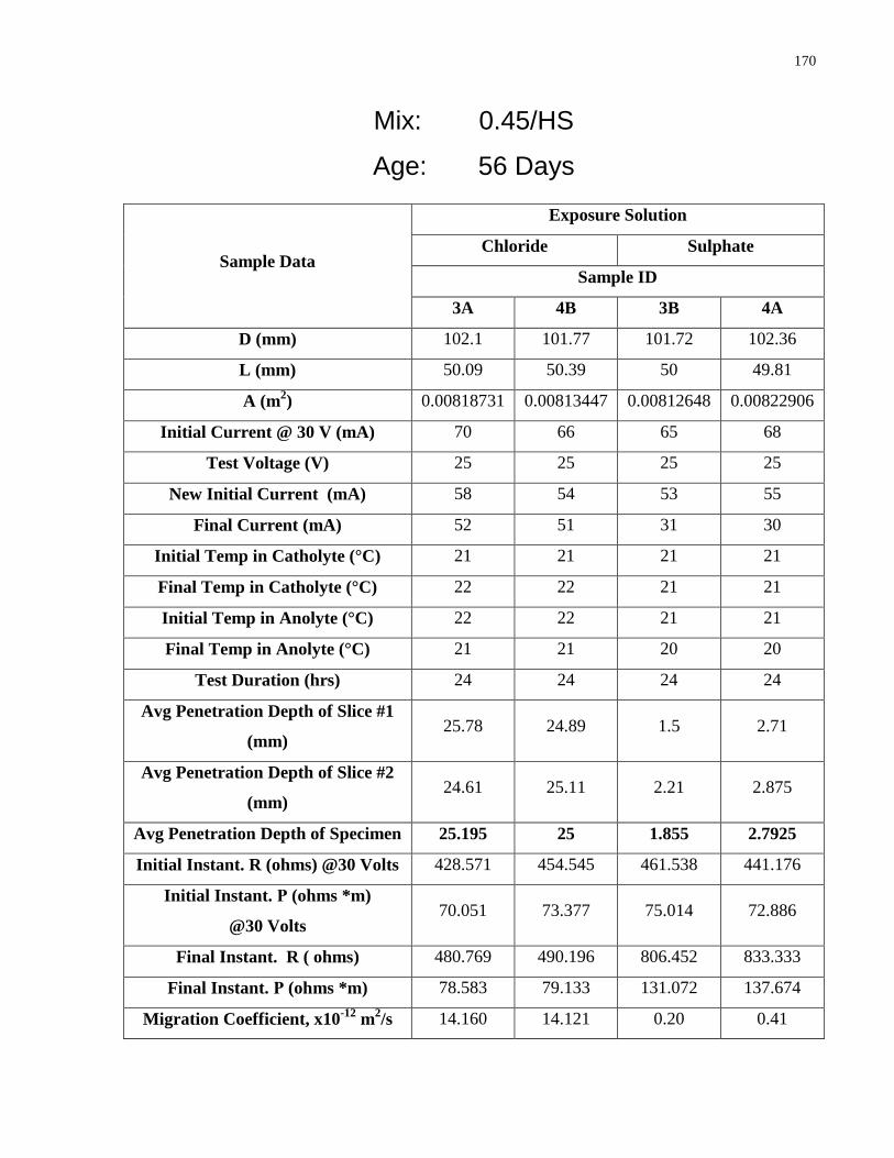
170
Mix: 0.45/HS
Age: 56 Days
Sample Data
Exposure Solution
Chloride Sulphate
Sample ID
3A 4B 3B 4A
D (mm) 102.1 101.77 101.72 102.36
L (mm) 50.09 50.39 50 49.81
A (m2) 0.00818731 0.00813447 0.00812648 0.00822906
Initial Current @ 30 V (mA) 70 66 65 68
Test Voltage (V) 25 25 25 25
New Initial Current (mA) 58 54 53 55
Final Current (mA) 52 51 31 30
Initial Temp in Catholyte (°C) 21 21 21 21
Final Temp in Catholyte (°C) 22 22 21 21
Initial Temp in Anolyte (°C) 22 22 21 21
Final Temp in Anolyte (°C) 21 21 20 20
Test Duration (hrs) 24 24 24 24
Avg Penetration Depth of Slice #1
(mm) 25.78 24.89 1.5 2.71
Avg Penetration Depth of Slice #2
(mm) 24.61 25.11 2.21 2.875
Avg Penetration Depth of Specimen 25.195 25 1.855 2.7925
Initial Instant. R (ohms) @30 Volts 428.571 454.545 461.538 441.176
Initial Instant. Ρ (ohms *m)
@30 Volts 70.051 73.377 75.014 72.886
Final Instant. R ( ohms) 480.769 490.196 806.452 833.333
Final Instant. Ρ (ohms *m) 78.583 79.133 131.072 137.674
Migration Coefficient, x10-12 m2/s 14.160 14.121 0.20 0.41

171
Mix: 0.4/HS
Age: 35 Days
Sample Data
Exposure Solution
Chloride Sulphate
Sample ID
3A 4B 3B 4A
D (mm) 101.75 101.41 101.84 101.88
L (mm) 51.17 51.27 51.28 50.96
A (m2) 0.00813128 0.00807703 0.00814567 0.00815207
Initial Current @ 30 V (mA) 69 66 65 66.5
Test Voltage (V) 25 25 25 25
New Initial Current (mA) 56 53 53.5 55
Final Current (mA) 51 48 26 24
Initial Temp in Catholyte (°C) 20 °C 20 °C 20 °C 20 °C
Final Temp in Catholyte (°C) 21 °C 21 °C 20 °C 20 °C
Initial Temp in Anolyte (°C) 21 21 21 21
Final Temp in Anolyte (°C) 20.5 20.5 19.5 19.5
Test Duration (hrs) 24 24 24 24
Avg Penetration Depth of Slice #1
(mm) 24.43 21 0.89 0.92
Avg Penetration Depth of Slice #2
(mm) 21.07 23.125 1.5 0.95
Avg Penetration Depth of Specimen 22.75 22.0625 1.195 0.935
Initial Instant. R (ohms) @30 Volts 434.783 454.545 461.538 451.128
Initial Instant. ρ (ohms *m)
@30 Volts 69.090 71.609 73.314 72.167
Final Instant. R ( ohms) 490.196 520.833 961.538 1041.667
Final Instant. ρ (ohms *m) 77.896 82.052 152.737 166.635
Migration Coefficient, x10-12 m2/s 12.917 12.5211 0.07 0.02

172
Mix: 0.4/HS
Age: 56 Days
Sample Data
Exposure Solution
Chloride Sulphate
Sample ID
3A 4B 3B 4A
D (mm) 102.05 101.11 101.82 101.93
L (mm) 50.03 49.58 49.64 49.77
A (m2) 0.00817930 0.00802931 0.00814247 0.00816007
Initial Current @ 30 V (mA) 57 68 59.5 58
Test Voltage (V) 30 25 30 30
New Initial Current (mA) 55 56 59.5 58
Final Current (mA) 51 49 21 20
Initial Temp in Catholyte (°C) 21 21 21 21
Final Temp in Catholyte (°C) 21 21 21 21
Initial Temp in Anolyte (°C) 21 21 21.5 21.5
Final Temp in Anolyte (°C) 21 21 20 20
Test Duration (hrs) 24 24 24 24
Avg Penetration Depth of Slice #1
(mm) 21.64 22.17 2.25 1.66
Avg Penetration Depth of Slice #2
(mm) 21.1 21.44 1.79
Avg Penetration Depth of Specimen 21.37 21.44 2.02 1.66
Initial Instant. R (ohms) @30 Volts 526.316 441.176 504.202 517.241
Initial Instant. ρ (ohms *m)
@30 Volts 86.046 71.447 82.704 84.805
Final Instant. R ( ohms) 588.235 510.204 1428.571 1428.571
Final Instant. ρ (ohms *m) 96.169 82.626 234.329 234.222
Migration Coefficient, x10-12 m2/s 9.860 11.780 0.23 0.16

173
Mix: 0.5/MS
Age: 35 Days
Sample Data
Exposure Solution
Chloride Sulphate
Sample ID
3A 4B 3B 4A
D (mm) 102.12 102.08 101.72 101.72
L (mm) 50.02 51.04 51.36 51.16
A (m2) 0.00819052 0.00818411 0.00812648 0.00812648
Initial Current @ 30 V (mA) 79 77.5 67 74
Test Voltage (V) 25 25 25 25
New Initial Current (mA) 65 63 55 61
Final Current (mA) 62.5 58 19 17
Initial Temp in Catholyte (°C) 22 °C 22 °C 22 °C 22 °C
Final Temp in Catholyte (°C) 22 °C 22 °C 21 °C 21 °C
Initial Temp in Anolyte (°C) 22 22 22 22
Final Temp in Anolyte (°C) 22 22 20 20
Test Duration (hrs) 24 24 24 24
Avg Penetration Depth of Slice #1
(mm) 35.57 31.83 2.56 2.59
Avg Penetration Depth of Slice #2
(mm) 32.94 29.28 3.11 2.24
Avg Penetration Depth of Specimen 34.255 30.555 2.835 2.415
Initial Instant. R (ohms) @30 Volts 379.747 387.097 447.761 405.405
Initial Instant. ρ (ohms *m)
@30 Volts 62.182 62.070 70.847 64.396
Final Instant. R ( ohms) 400.000 431.034 1315.789 1470.588
Final Instant. ρ (ohms *m) 65.498 69.115 208.192 233.595
Migration Coefficient, x10-12 m2/s 19.631 17.725 0.43 0.33
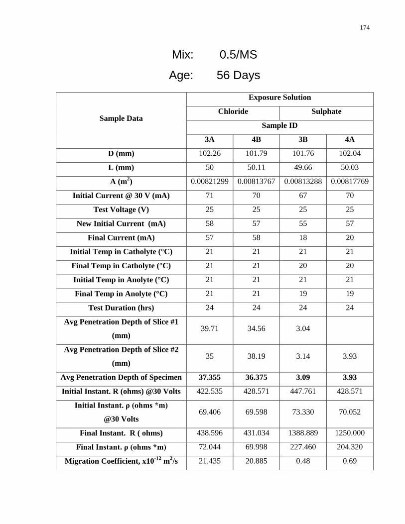
174
Mix: 0.5/MS
Age: 56 Days
Sample Data
Exposure Solution
Chloride Sulphate
Sample ID
3A 4B 3B 4A
D (mm) 102.26 101.79 101.76 102.04
L (mm) 50 50.11 49.66 50.03
A (m2) 0.00821299 0.00813767 0.00813288 0.00817769
Initial Current @ 30 V (mA) 71 70 67 70
Test Voltage (V) 25 25 25 25
New Initial Current (mA) 58 57 55 57
Final Current (mA) 57 58 18 20
Initial Temp in Catholyte (°C) 21 21 21 21
Final Temp in Catholyte (°C) 21 21 20 20
Initial Temp in Anolyte (°C) 21 21 21 21
Final Temp in Anolyte (°C) 21 21 19 19
Test Duration (hrs) 24 24 24 24
Avg Penetration Depth of Slice #1
(mm) 39.71 34.56 3.04
Avg Penetration Depth of Slice #2
(mm) 35 38.19 3.14 3.93
Avg Penetration Depth of Specimen 37.355 36.375 3.09 3.93
Initial Instant. R (ohms) @30 Volts 422.535 428.571 447.761 428.571
Initial Instant. ρ (ohms *m)
@30 Volts 69.406 69.598 73.330 70.052
Final Instant. R ( ohms) 438.596 431.034 1388.889 1250.000
Final Instant. ρ (ohms *m) 72.044 69.998 227.460 204.320
Migration Coefficient, x10-12 m2/s 21.435 20.885 0.48 0.69

175
Mix: 0.4/MS/50S
Age: 35 Days
Sample Data
Exposure Solution
Chloride Sulphate
Sample ID
3A 4B 3B 4A
D (mm) 102.24 101.77 101.89 102.06
L (mm) 50.19 49.9 49.98 50.26
A (m2) 0.00820978 0.00813447 0.00815367 0.00818090
Initial Current @ 30 V (mA) 23 24 23 23
Test Voltage (V) 40 40 40 40
New Initial Current (mA) 31 32 31 31
Final Current (mA) 27 28 18 18
Initial Temp in Catholyte (°C) 22 °C 22 °C 21 °C 21 °C
Final Temp in Catholyte (°C) 21 °C 21 °C 20 °C 20 °C
Initial Temp in Anolyte (°C) 22 22 22 22
Final Temp in Anolyte (°C) 20.5 20.5 20 20
Test Duration (hrs) 24 24 24 24
Avg Penetration Depth of Slice #1
(mm) 8.89 27.31 1.27 1.19
Avg Penetration Depth of Slice #2
(mm) 9 26.69 1.44 1.2
Avg Penetration Depth of Specimen 8.945 27 1.355 1.195
Initial Instant. R (ohms) @30 Volts 1304.348 1250.000 1304.348 1304.348
Initial Instant. ρ (ohms *m)
@30 Volts 213.357 203.769 212.789 212.311
Final Instant. R ( ohms) 1481.481 1428.571 2222.222 2222.222
Final Instant. ρ (ohms *m) 242.332 232.879 362.530 361.715
Migration Coefficient, x10-12 m2/s 2.919 9.454 0.10 0.08
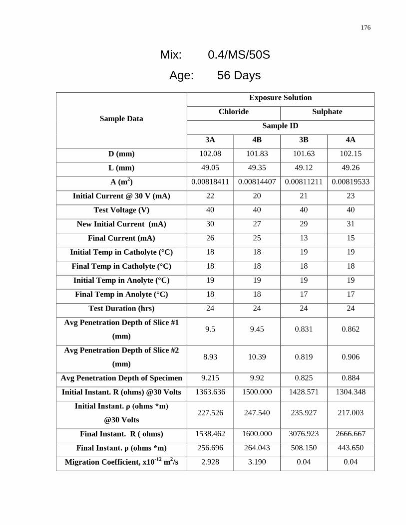
176
Mix: 0.4/MS/50S
Age: 56 Days
Sample Data
Exposure Solution
Chloride Sulphate
Sample ID
3A 4B 3B 4A
D (mm) 102.08 101.83 101.63 102.15
L (mm) 49.05 49.35 49.12 49.26
A (m2) 0.00818411 0.00814407 0.00811211 0.00819533
Initial Current @ 30 V (mA) 22 20 21 23
Test Voltage (V) 40 40 40 40
New Initial Current (mA) 30 27 29 31
Final Current (mA) 26 25 13 15
Initial Temp in Catholyte (°C) 18 18 19 19
Final Temp in Catholyte (°C) 18 18 18 18
Initial Temp in Anolyte (°C) 19 19 19 19
Final Temp in Anolyte (°C) 18 18 17 17
Test Duration (hrs) 24 24 24 24
Avg Penetration Depth of Slice #1
(mm) 9.5 9.45 0.831 0.862
Avg Penetration Depth of Slice #2
(mm) 8.93 10.39 0.819 0.906
Avg Penetration Depth of Specimen 9.215 9.92 0.825 0.884
Initial Instant. R (ohms) @30 Volts 1363.636 1500.000 1428.571 1304.348
Initial Instant. ρ (ohms *m)
@30 Volts 227.526 247.540 235.927 217.003
Final Instant. R ( ohms) 1538.462 1600.000 3076.923 2666.667
Final Instant. ρ (ohms *m) 256.696 264.043 508.150 443.650
Migration Coefficient, x10-12 m2/s 2.928 3.190 0.04 0.04

177
Appendix E Merlin and Monfore Electrical Resistivity Data

178
Merlin Electrical Resistivity
𝑈𝑛𝑖𝑡𝑠: 𝑜ℎ𝑚𝑠 ∙ 𝑚
Mix ID
Age : 35
Test Method
ASTM C 1202 NT Build 492
Exposure Solution
Chloride Sulphate Chloride Sulphate
Sample ID
1A 2B 1B 2A 3A 4B 3B 4A
0.5/GU/35 Pre Test 139.42 141.78 130.23 150.51 130.18 135.86 144.82 145.29
Post Test 134.01 135.35 134.85 139.92 138.02 146.54 173.48 180.12
0.5/GU Pre Test 56.067 58.967 51.498 56.001 51.917 56.262 56.489 55.463
Post Test 66.285 74.398 60.378 72.018 64.912 68.564 77.235 82.427
0.45/GU/50 Pre Test 195.12 216.7 206.57 191.37 199.08 187.17 210.47 203.11
Post Test 196.46 189.7 205.55 189.6 189.42 150.92 242.11 238.46
0. 4/GU/50 Pre Test 184.07 183.32 197.43 191.37 187.64 195.23 186.28 181.45
Post Test 178.05 182.06 204.84 198.76 185.6 185.21 219.48 226.7
0.5/InterCem Pre Test 142.47 152.67 147.45 139.71 135.79 145.48 138.9 163.22
Post Test 140.05 152.47 152.07 151.77 131.82 136.79 170.92 196.55
0.45/HS Pre Test 43.14 44.886 42.488 44.33 48.332 49.125 47.405 44.45
Post Test 48.752 52.858 49.682 52.426 50.982 50.106 59.067 60.75
0.4/HS Pre Test 51.406 49.035 50.261 51.251 50.707 51.433 51.467 51.158
Post Test 51.747 51.919 51.02 53.472 56.062 57.266 61.373 58.275
0.5/MS Pre Test 51.406 47.127 49.298 45.967 44.171 44.901 51.766 44.651
Post Test 54.855 49.477 54.308 54.51 49.242 50.761 63.18 65.273
0.4/MS/50 Pre Test 164.84 178.09 173.62 162.03 188.35 184.46 183.94 181.11
Post Test 173.06 172.3 172.27 175.68 191.93 189.39 208.72 221.46

179
Merlin Electrical Resistivity
𝑈𝑛𝑖𝑡𝑠: 𝑜ℎ𝑚𝑠 ∙ 𝑚
Mix ID
Age : 56
Test Method
ASTM C 1202 NT Build 492
Exposure Solution
Chloride Sulphate Chloride Sulphate
Sample ID
1A 2B 1B 2A 3A 4B 3B 4A
0.5/GU/35 Pre Test 152.62 158.47 149.02 150.37 144.59 159.87 143.79 148.59
Post Test 150.73 159.31 154.55 161.72 151.31 151.59 194.84 193.24
0.5/GU Pre Test 66.1295 63.798 69.124 66.318 60.214 68.535 67.513 60.089
Post Test 72.184 68.803 75.282 73.315 66.338 75.975 85.707 79.415
0.45/GU/50 Pre Test 275.39 262.98 249.35 257.31 247.63 246.02 252.68 219.7
Post Test 231.64 243.72 220.71 228.24 189.45 206.09 266.64 253.96
0. 4/GU/50 Pre Test 227.08 237.57 224.58 227.95 225.32 212.06 227.42 229.39
Post Test 223 224.47 221.38 221.1 211.95 219.67 328.71 273.95
0.5/InterCem Pre Test 260.67 241.37 239.3 242.99 248.26 224.87 265.75 238.67
Post Test 231.91 237.61 269.33 249.1 184.77 186.68 278.4 304.57
0.45/HS Pre Test 54.224 49.728 59.918 47.493 53.485 58.454 56.796 54.583
Post Test 58.502 53.735 63.808 53.559 58.832 58.5 73.526 73.486
0.4/HS Pre Test 54.802 58.073 59.143 55.014 63.87 55.235 63.701 66.084
Post Test 60.93 61.983 65.85 66.62 68.366 58.892 78.908 82.262
0.5/MS Pre Test 49.676 55.344 54.492 56.245 51.356 47.026 48.36 46.188
Post Test 50.759 54.492 51.9 55.044 51.484 49.416 62.405 63.503
0.4/MS/50 Pre Test 202.82 207.79 212.75 203.64 199.13 228.5 208.2 197.55
Post Test 178 169.05 184.51 178.13 184.58 195.13 209.65 198.41

180
Monfore Bulk Electrical Resistivity
𝑈𝑛𝑖𝑡𝑠: 𝑜ℎ𝑚𝑠 ∙ 𝑚
Mix ID
Age : 35
Test Method
ASTM C 1202 NT Build 492
Exposure Solution
Chloride Sulphate Chloride Sulphate
Sample ID
1A 2B 1B 2A 3A 4B 3B 4A
0.5/GU/35 Pre Test 220.93 237.77 244.93 218.64 218.41 185.31 188.51 188.74
Post Test 199.35 197.67 204.39 221.04 227.99 194.26 271.20 297.75
0.5/GU Pre Test 142.28 108.54 111.30 98.07 126.43 116.72 140.06 163.66
Post Test 173.17 112.16 112.76 114.18 98.32 105.04 194.28 243.98
0.45/GU/50 Pre Test 304.91 340.04 316.73 475.81 282.68 269.41 291.56 275.43
Post Test 262.15 259.25 268.41 253.39 294.77 251.22 312.84 317.74
0. 4/GU/50 Pre Test 340.91 482.87 377.77 374.22 277.85 385.70 309.91 330.76
Post Test 303.41 403.04 275.45 402.66 287.31 284.64 311.31 393.19
0.5/InterCem Pre Test 282.93 395.21 231.95 279.50 324.53 394.94 281.49 483.97
Post Test 207.08 244.53 210.23 239.10 222.38 262.48 288.54 304.95
0.45/HS Pre Test 127.92 107.75 107.39 103.20 122.88 95.10 101.13 91.49
Post Test 73.33 73.43 78.35 78.12 92.89 85.11 103.70 114.44
0.4/HS Pre Test 104.82 108.27 115.00 116.14 100.17 117.97 121.36 97.85
Post Test 80.27 87.06 84.92 106.88 84.43 90.39 99.77 105.00
0.5/MS Pre Test 111.57 92.40 112.94 95.57 94.12 89.21 99.71 92.70
Post Test 84.88 70.20 83.29 80.72 81.48 79.29 98.60 96.62
0.4/MS/50 Pre Test 285.96 258.63 289.48 249.88 246.22 249.13 248.11 255.00
Post Test 209.56 218.06 228.87 214.15 233.42 220.16 292.58 287.34

181
Monfore Bulk Electrical Resistivity
𝑈𝑛𝑖𝑡𝑠: 𝑜ℎ𝑚𝑠 ∙ 𝑚
Mix ID
Age : 56
Test Method
ASTM C 1202 NT Build 492
Exposure Solution
Chloride Sulphate Chloride Sulphate
Sample ID
1A 2B 1B 2A 3A 4B 3B 4A
0.5/GU/35 Pre Test 389.72 290.15 425.66 269.50 324.93 331.87 238.88 404.51 Post Test 229.08 200.97 224.90 250.69 304.53 419.26 459.68 468.55
0.5/GU Pre Test 168.16 124.04 125.52 121.18 103.32 124.52 115.39 102.92 Post Test 138.39 113.21 118.15 121.75 99.34 186.36 178.98 142.66
0.45/GU/50 Pre Test 497.65 433.55 554.89 480.64 365.96 349.18 412.38 328.09 Post Test 286.42 338.28 289.28 357.66 325.33 298.64 361.95 376.05
0. 4/GU/50 Pre Test 326.70 392.53 403.43 428.41 358.50 307.92 329.58 405.39 Post Test 270.35 312.68 310.68 289.07 287.08 285.27 370.44 360.36
0.5/InterCem Pre Test 450.24 391.08 368.14 412.96 373.47 331.95 354.36 327.10 Post Test 314.60 321.53 281.54 331.17 308.58 294.80 360.18 375.50
0.45/HS Pre Test 95.61 83.63 108.23 82.66 58.36 70.14 68.56 64.24 Post Test 82.62 76.07 89.69 80.30 84.19 81.21 119.12 119.38
0.4/HS Pre Test 105.93 109.06 109.46 109.28 117.79 97.07 113.08 110.54 Post Test 89.27 67.98 73.49 72.51 95.99 88.01 120.74 122.37
0.5/MS Pre Test 85.67 99.45 87.64 95.87 90.85 90.27 93.50 87.83 Post Test 77.25 84.77 79.83 87.35 55.32 78.19 135.26 133.43
0.4/MS/50 Pre Test 332.29 335.25 345.89 321.62 294.28 304.61 299.04 301.25 Post Test 248.75 232.71 272.89 269.90 283.86 298.24 324.82 289.81

182
Appendix F Sulphate Profile Grinding and ICP Data

183
Sample Details : 0.5 w/cm
GU cement with 35% Slag 6.5 months old
Tested in modified NT Build 492 - 10% Sodium Sulphate
Test duration: 4 Days
Blank Concentration, mg/l
BDL = below detection limit
Na+ K+ Ca+2 S- 0.06 0.02 0.61 BDL
Depth
( mm)
Large Beaker
Mass
(g)
Sample
Mass (g)
Filtered
Mass (g)
Element concentration, mg/L Element concentration (adjusted with blank), mg/g
Na K Ca S Na K Ca S
0.381 111.23 2.0241 198.1332 16.62 19.59 4346.06 206.92 0.71 0.84 186.57 8.88 1.143 111.27 1.9755 199.3850 14.16 22.31 4301.40 168.38 0.63 0.99 191.84 7.51 1.905 121.10 1.9953 205.4227 17.11 30.83 4433.84 131.24 0.72 1.30 187.36 5.55 2.667 104.65 2.0146 186.7517 18.81 38.43 4515.13 107.90 0.76 1.57 183.98 4.40 3.429 113.66 2.0083 191.6199 21.58 46.34 4565.62 88.70 0.84 1.80 177.22 3.44 4.191 112.41 1.9915 218.8700 15.57 32.62 4018.18 79.76 0.83 1.74 214.77 4.26 4.953 112.66 2.0265 195.1658 21.61 45.43 4492.96 71.83 0.88 1.85 182.89 2.92 5.715 105.40 2.0244 197.7710 17.78 39.65 4342.00 62.38 0.81 1.81 198.10 2.85 6.477 111.05 2.0201 191.1620 21.92 45.67 4553.63 51.17 0.87 1.81 180.55 2.03 7.239 105.11 1.9843 192.4043 19.17 39.58 4390.23 45.46 0.84 1.74 193.12 2.00 8.001 118.21 1.9884 207.2981 18.81 37.23 4354.73 38.27 0.84 1.67 195.09 1.71 8.763 111.57 2.0158 190.1323 23.09 46.82 4551.63 42.26 0.90 1.82 177.36 1.65 9.525 112.93 2.0051 202.7686 18.43 36.03 4355.27 34.44 0.82 1.61 195.11 1.54

184
Sample Details : 0.4 w/cm 100% HS cement
56 Days old Tested in modified NT Build 492 - 10% Sodium Sulphate
Test Duration: 24 hours
Depth
( mm)
Large Beaker
Mass
(g)
Sample
Mass
(g)
Filtered
Mass (g)
Element concentration, mg/L Element concentration (adjusted with blank), mg/g
Na K Ca S Na K Ca S
0.381 107.20 1.9803 194.8500 21.18 14.96 4113.13 214.63 0.93 0.64 182.04 9.48 1.143 109.30 2.0077 188.2500 11.46 13.43 4676.74 142.64 0.44 0.51 183.9 5.61 1.905 107.58 1.9711 204.9000 8.3 10.5 3900.48 67.31 0.40 0.50 192.56 3.32 2.667 122.26 1.9973 204.0100 9.65 13.00 4404.82 58.25 0.39 0.52 180.28 2.38 3.429 101.95 1.9970 194.8200 8.65 11.26 4070.85 41.8 0.39 0.51 189.3 1.94 4.191 107.68 1.9704 210.2400 7.95 10.46 3838.96 34.71 0.40 0.52 199.79 1.80 4.953 105.83 1.9610 202.7100 8.72 11.07 3899.88 33.78 0.42 0.53 192.65 1.67 5.715 106.19 1.9575 196.5400 9.36 12.28 4244.5 35.24 0.42 0.55 195.9 1.62 6.477 104.23 2.0118 204.5700 8.63 11.98 3913.64 32.75 0.42 0.58 195.18 1.63
Determining the change in the Total Sulphur Concentration of profile ground concrete
sample
For each layer:
𝐶𝑜𝑛𝑐𝑒𝑛𝑡𝑟𝑎𝑡𝑖𝑜𝑛,𝑚𝑖𝑙𝑙𝑖𝑔𝑟𝑎𝑚𝑠 𝑜𝑓 𝑒𝑙𝑒𝑚𝑒𝑛𝑡
𝑔𝑟𝑎𝑚𝑠 𝑜𝑓 𝑐𝑜𝑛𝑐𝑟𝑒𝑡𝑒 𝑝𝑜𝑤𝑑𝑒𝑟
= 𝑐𝑜𝑛𝑐𝑒𝑛𝑡𝑟𝑎𝑡𝑖𝑜𝑛 �𝑚𝑔 𝑜𝑓 𝑒𝑙𝑒𝑚𝑒𝑛𝑡𝐿 𝑜𝑓 𝑠𝑜𝑙𝑢𝑡𝑖𝑜𝑛
� ×1 𝐿
1000 𝑚𝑙 × 𝑚𝑎𝑠𝑠 𝑜𝑓 𝑠𝑜𝑙𝑢𝑡𝑖𝑜𝑛 (𝑔)
× 1𝜌𝑤
×1
𝑚𝑎𝑠𝑠 𝑜𝑓 𝑝𝑜𝑤𝑑𝑒𝑟𝑒𝑑 𝑠𝑎𝑚𝑝𝑙𝑒 (𝑔)
Sample Calculation
Sample Details:
0.5 w/cm; GU cement with 35% slag replacement

185
Age: 6.5 months
Test: modified NT Build 492 – 10% Na2SO4
Test Duration: 4 Days
2nd layer, 1.143mm deep.
Mass of Beaker Containing the solution, g: 111.2649 g
Mass of Filtered Solution, g: 199.13850 g
Mass of concrete powder, g: 1.9755 g
Sulphur Concentration, mg/ L (adjusted with blank): 168.38 mg/L
Assumption: Volume of solution to mass of solution is 1: 1, or, assuming that the solution has
the density of water, 1g/ml.
Total Sulphur at 1.143 mm depth:
𝑆𝑢𝑙𝑝ℎ𝑢𝑟 𝐶𝑜𝑛𝑐𝑒𝑛𝑡𝑟𝑎𝑡𝑖𝑜𝑛,𝑚𝑖𝑙𝑙𝑖𝑔𝑟𝑎𝑚𝑠 𝑜𝑓 𝑠𝑢𝑙𝑝ℎ𝑢𝑟
𝑔𝑟𝑎𝑚𝑠 𝑜𝑓 𝑐𝑜𝑛𝑐𝑟𝑒𝑡𝑒 𝑝𝑜𝑤𝑑𝑒𝑟
= 168.38 �𝑚𝑔 𝑜𝑓𝑠𝑢𝑙𝑝ℎ𝑢𝑟𝐿 𝑜𝑓 𝑠𝑜𝑙𝑢𝑡𝑖𝑜𝑛
� ×1 𝐿
1000 𝑚𝑙
× (199.3850 − 111.2649) 𝑔 𝑜𝑓 𝑠𝑜𝑙𝑢𝑡𝑖𝑜𝑛 × 1𝑚𝑙𝑔
×1
1.9755𝑔 𝑜𝑓 𝑐𝑜𝑛𝑐𝑟𝑒𝑡𝑒 𝑝𝑜𝑤𝑑𝑒𝑟= 7.51
𝑚𝑔 𝑜𝑓 𝑠𝑢𝑙𝑝ℎ𝑢𝑟𝑔 𝑜𝑓 𝑐𝑜𝑛𝑐𝑟𝑒𝑡𝑒 𝑝𝑜𝑤𝑑𝑒𝑟

186
Appendix G NT Build 492 Modified Test Duration Data

187
Change in current and voltage with test duration of 1 day, specimens were 6.5 months old of 0.5
w/cm and 100% GU cement. Note that specimens 1A and 1B were cut from the same cylinder
and specimens 2A and 2B were cut from the same cylinder.
Current (mA) Chloride-exposed
specimens1A
Voltage (V)Chloride-exposed
specimens
2BCurrent (mA) Sulphate-exposed
specimens 1B
Voltage (V) Sulphate-exposed
specimens
2A
20
25
30
35
40
45
50
55
60
65
70
75
80
0
10
20
30
40
50
60
70
80
0 4 9 14 19 24 28
Volta
ge A
pplie
d to
Spe
cim
en (V
)
Curr
ent (
mA)
Test Duration (Hours)

188
Change in current and voltage with test duration of 1 day, specimens were 6.5 months old of 0.5
w/cm and GU cement with 35% slag replacement. Note that specimens 1A and 1B were cut
from the same cylinder and specimens 2A and 2B were cut from the same cylinder.
Current (mA) Cloride-exposed
specimens1A
voltage (V) Sulphate exposed specimens
2B
Current (mA) Sulphate-exposed
specimens2A
Voltage (V)Sulphate exposed
specimens
1B
20
30
40
50
60
70
80
90
100
110
120
0
5
10
15
20
25
30
35
40
45
50
0 4 9 14 19 24 28
Volta
ge A
pplie
d to
Spe
cim
en (V
)
Curr
ent (
mA)
TestDuration (Hours)

189
Change in current and voltage with test duration of 4 days, specimens were 6.5 months old of 0.5
w/cm with 100% GU cement and, 0.5 w/cm and GU cement with 35% slag replacement.
Voltage (V) 0.5 w/cm 100% GU
Current (mA) 0.5 w/cm 100% GUSpecimen 4B (Top)
Specimen 3A (Bottom)
Voltage (V) 0.5 w/cm, GU with
35% Slag
Current (mA) 0.5 w/cm , GU with
35% SlagSpecimen 3A (Top)
Specimen 4B (Bottom)
25
45
65
85
105
125
145
0
5
10
15
20
25
30
35
40
45
0 1 2 3 4 5
Volta
ge A
pplie
d to
Spe
cim
ens (
V)
Curr
ent (
mA)
Test Duration (Days)

190
Change in current and voltage with test duration of 9 days, specimens were 6.5 months old of 0.5
w/cm with 100% GU cement and, 0.5 w/cm and GU cement with 35% slag replacement. Note
that Specimens 4A and 4B (in Figure F.3) were cut from the same cylinder, and specimens 3B
and 3A (in Figure F.3) were cut from the same cylinder.
Voltage (V) 0.5 w/cm, 100% GU
Current (mA) 0.5 w/cm,100% GUSpecimen 4A (Top)
Specimen 3B (Bottom)
Voltage (V)0.5 w/cm, GU with
35% Slag
Current (mA)0.5 w/cm, GU with
35% Slag; Specimen 3B (Top)
Specimen 4A (Bottom, noisy line)
0
10
20
30
40
50
0
10
20
30
40
50
60
70
80
90
0 1 2 3 4 5 6 7 8 9 10
Volta
ge A
pplie
d to
Spe
cim
en (V
)
Curr
ent (
mA)
Test Duration (Days)

191
Mix ID: T3
Mix Properties: 0.5 w/cm 100% GU cement
Age: 6.5 months
Sample Data
Exposure Solution
Chloride Sulphate
Sample ID
1A 2B 2A 1B
D (mm) 102.105 101.77 102.06 101.69
L (mm) 50.415 50.61 50.485 50.72
A (m2) 0.00818811 0.00813447 0.00818090 0.00812169
Initial Current @ 30 V (mA) 50 47 37 35
Average Applied Test Voltage (V) 25.18 25.47 32.02 31.84
New Initial Current (mA) 50 47 41 43
Final Current (mA) 47 45 24 25
Initial Temp in Catholyte (°C) 19 19 19 19
Final Temp in Catholyte (°C) 18 18 19 19
Initial Temp in Anolyte (°C) 19 19 20 20
Final Temp in Anolyte (°C) 18 18 19 19
Test Duration (hrs) 24 24 24 24
Avg Penetration Depth of Slice #1
(mm) 14.72 16.83 1.5 1.34
Avg Penetration Depth of Slice #2
(mm) 15.33 15.92 1.56 1.31
Avg Penetration Depth of Specimen 15.025 16.375 1.53 1.325
Migration Coefficient, x10-12 m2/s 8.02 8.74 0.14 0.10
Total Charge Passing (Coulombs) 4033 3805 2512 2668

192
Mix ID: T3
Mix Properties: 0.5 w/cm 100% GU cement
Age: 6.5 months
Sample Data
Exposure Solution
Sulphate
Sample ID
3A 4B 4A 3B
D (mm) 102.18 102.03 102.245 101.7025
L (mm) 50.64 50.56 50.27 50.94
A (m2) 0.00820015 0.00817609 0.008211 0.008124
Initial Current @ 30 V (mA) 32 34 37 32
Average Applied Test Voltage (V) 33.43 33.25 33.50 33.59
New Initial Current (mA) 38 40 43 37
Final Current (mA) 9 11 7 6
Initial Temp in Catholyte (°C) 18.5 18.5 21.5 21.5
Final Temp in Catholyte (°C) 22 22 23.5 23.5
Initial Temp in Anolyte (°C) 18 18 21 21
Final Temp in Anolyte (°C) 21 21 23.5 23.5
Test Duration (hrs) 92.58 92.58 214 214
Avg Penetration Depth of Slice #1
(mm) 2.61 2.39 4.14 2.89
Avg Penetration Depth of Slice #2
(mm) 1.95 2.29 5.07 4.6
Avg Penetration Depth of Specimen 2.28 2.34 4.605 3.745
Migration Coefficient, x10-12 m2/s 0.07 0.07 0.08 0.06
Total Charge Passing (Coulombs) 5213 5822 11528 10813

193
Mix ID: T5
Mix Properties: 0.5 w/cm GU cement with 35% slag replacement
Age: 6.5 month
Sample Data
Exposure Solution
Chloride Sulphate
Sample ID
1A 2B 2A 1B
D (mm) 102.06 101.65 102.17 101.97
L (mm) 49.675 50.545 50.965 50.77
A (m2) 0.00818090 0.00811530 0.00819854 0.00816648
Initial Current @ 30 V (mA) 40 31 17 16
Average Applied Test Voltage (V) 30.80 30.81 48.05 48.05
New Initial Current (mA) 47 36.5 29 27
Final Current (mA) 41 46 16 16
Initial Temp in Catholyte (°C) 21 21 20 20
Final Temp in Catholyte (°C) 23 23 22 22
Initial Temp in Anolyte (°C) 20 20 20 20
Final Temp in Anolyte (°C) 23 23 22 22
Test Duration (hrs) 24 24 24 24
Avg Penetration Depth of Slice #1
(mm) 6.375 7.8 1.01 1.3625
Avg Penetration Depth of Slice #2
(mm) 6.75 7.57 0.92 1.22
Avg Penetration Depth of Specimen 6.56 7.69 0.97 1.29125
Migration Coefficient, x10-12 m2/s 2.6 3.2 0.05 0.09
Total Charge Passing (Coulombs) 3525 3502 1645 1644

194
Mix ID: T5
Mix Properties: 0.5 w/cm GU cement with 35% slag replacement
Age: 6.5 months
Sample Data
Exposure Solution
Sulphate
Sample ID
3A 4B 4A 3B
D (mm) 102.23 101.87 102.155 102.005
L (mm) 50.49 50.99 50.58 50.47
A (m2) 0.00820818 0.00815047 0.008196 0.008172
Initial Current @ 30 V (mA) 19 16 16 18
Average Applied Test Voltage (V) 48.48 48.57 48.46 48.67
New Initial Current (mA) 31.12 27.31 28 30
Final Current (mA) 11 10 9 9
Initial Temp in Catholyte (°C) 19 19 25 25
Final Temp in Catholyte (°C) 18 18 24.6 24.6
Initial Temp in Anolyte (°C) 20 20 23 23
Final Temp in Anolyte (°C) 18 18 24.6 24.6
Test Duration (hrs) 92.33 92.33 213.75 213.75
Avg Penetration Depth of Slice #1
(mm) 2.96 3.3125 4.04 4.29
Avg Penetration Depth of Slice #2
(mm) 3.25 3.31 4.36 4.375
Avg Penetration Depth of Specimen 3.105 3.31125 4.2 4.3325
Migration Coefficient, x10-12 m2/s 0.08 0.09 0.05 0.05
Total Charge Passing (Coulombs) 5057 4757 11842 10236

195
Appendix H Compressive Strengths

196
Mix ID Age (Days) Peak Load (KN) ø (mm) H (mm) Area (mm2)
Peak
Stress
(MPa)
0.5/GU/35 7 201 101.83 194.00 8144.47 24.68
28 255.4 102.14 190.75 8192.93 31.17
0.5/GU 7 228.6 102.16 193.50 8196.54 27.89
28 275.3 101.85 191.75 8146.87 33.79
0.45/GU/50 7 235.8 101.68 188.75 8119.29 29.04
28 326.1 101.76 190.25 8133.07 40.10
0. 4/GU/50 8 274.2 101.80 191.50 8138.47 33.69
28 320.47 102.06 193.00 8180.10 39.18
0.5/InterCem 7 189.9 101.87 192.00 8149.67 23.30
28 305.5 101.74 191.75 8128.88 37.58
0.45/HS 7 208.5 101.63 191.25 8111.71 25.70
28 214.8 101.76 190.75 8133.27 26.41
0.4/HS 7 306.3 101.74 189.00 8130.08 37.67
28 274.1 101.58 190.75 8104.53 33.82
0.5/MS 7 268.1 101.79 188.25 8136.87 32.95
28 247.2 101.81 188.75 8140.47 30.37
0.4/MS/50 7 345.3 101.37 189.38 8070.65 42.78
28 347.08 101.59 188.00 8105.52 42.82