Agricultural Systems 99 (2009) 23–34

Contents lists available at ScienceDirect

Agricultural Systems

journal homepage: www.elsevier .com/ locate/agsy

Developing decision support tools for rangeland management by combiningstate and transition models and Bayesian belief networks

H. Bashari a,*, C. Smith b, O.J.H. Bosch b

a Department of Natural Resources, Isfahan University of Technology, Isfahan, Iranb School of Natural and Rural Systems Management, The University of Queensland, Gatton, QLD 4343, Australia

a r t i c l e i n f o

Article history:Received 8 August 2007Received in revised form 31 August 2008Accepted 5 September 2008Available online 1 November 2008

Keywords:Rangeland managementState and transition modelQueenslandBayesian belief networkAdaptive managementDecision support

0308-521X/$ - see front matter � 2008 Elsevier Ltd. Adoi:10.1016/j.agsy.2008.09.003

* Corresponding author. Tel.: +98 261 3410169/912E-mail address: H_bashari2001@yahoo.com (H. Ba

a b s t r a c t

State and transition models provide a simple and versatile way of describing vegetation dynamics inrangelands. However, state and transition models are traditionally descriptive, which has limited theirpractical application to rangeland management decision support. This paper demonstrates an approachto rangeland management decision support that combines a state and transition model with a Bayesianbelief network to provide a relatively simple and updatable rangeland dynamics model that can accom-modate uncertainty and be used for scenario, diagnostic, and sensitivity analysis. A state and transitionmodel, developed by the authors for subtropical grassland in south-east Queensland, Australia, is usedas an example. From the state and transition model, an influence diagram was built to show the pos-sible transitions among states and the factors influencing each transition. The influence diagram waspopulated with probabilities to produce a predictive model in the form of a Bayesian belief network.The behaviour of the model was tested using scenario and sensitivity analysis, revealing that selectivegrazing, grazing pressure, and soil nutrition were believed to influence most transitions, while fire fre-quency and the frequency of good wet seasons were also important in some transitions. Overall, theintegration of a state and transition model with a Bayesian belief network provided a useful way to uti-lise the knowledge embedded in a state and transition model for predictive purposes. Using a Bayesianbelief network in the modelling approach allowed uncertainty and variability to be explicitly accommo-dated in the modelling process, and expert knowledge to be utilised in model development. The meth-ods used also supported learning from monitoring data, thereby supporting adaptive rangelandmanagement.

� 2008 Elsevier Ltd. All rights reserved.

1. Introduction decision support tools), and using participatory methods to build

Many decision support tools have been developed by research-ers for the purpose of predicting the outcomes of rangeland man-agement decisions (see National Land and Water Resources Audit(2004) for those developed in Australia). However, many of thesetools failed to be adopted by rangeland managers. There may beseveral reasons for this, such as a lack of credibility in, or a per-ceived lack of usefulness of, decision support tools; a resistanceamong managers to replace their own decision-making processes,knowledge, and experience with decision support tools; the highcost of developing and maintaining decision support tools (particu-larly those that are data hungry and computationally intensive);and the need for decision support tools to compete with consultantsand advisors who are trusted and socially integrated with managers(Matthews et al., 2005). Efforts to overcome these barriers to adop-tion have included the testing of models, improving the cost effec-tiveness of decision support tools (developing low cost, low-data

ll rights reserved.

7474208.shari).

decision support tools (building decision support tools with manag-ers rather than for them) (Lynam, 2001; Smith et al., 2007a).

State and transition models (STMs) have traditionally provideda simple, versatile, and low cost means for developing rangelanddynamics models. They have been used by researchers in manyrangeland ecosystems to integrate knowledge about vegetationdynamics and the possible responses of vegetation to managementactions and environmental events (Friedel, 1991; Laycock, 1991;Hall et al., 1994; Allen-Diaz and Bartolome, 1998; Phelps andBosch, 2002). STMs generally describe vegetation dynamics usingdiagrams that position vegetation states along several axes repre-senting environmental or management gradients (such as grazingpressure). Possible transitions between these vegetation statesare represented using arrows, and a table, called a catalogue oftransitions, is used to describe the environmental or managementconditions under which each transition can occur.

Because of their graphical and descriptive nature, STMs areexcellent tools for communicating knowledge about rangelanddynamics between scientists, managers, and policy makers(Ludwig et al., 1996), and for allowing managers to identify

24 H. Bashari et al. / Agricultural Systems 99 (2009) 23–34

opportunities (environmental conditions and management op-tions) that may lead to favourable transitions (such as an improve-ment in pasture composition) or avoid circumstances likely totrigger unfavourable or irreversible transitions (such as pasturedegradation, soil erosion, or the invasion of weeds). However, be-cause they are essentially descriptive diagrams, one shortcomingof STMs is their limited predictive capability, which has restrictedtheir practical application in scenario analysis. Another shortcom-ing of STMs is related to their coarse handling of uncertainty,which in the past has been accommodated using qualitativedescriptions of transition probability such as ‘‘high”, ‘‘moderate”,and ‘‘low” (Orr et al., 1994).

Both predictive ability and the ability to accommodate uncer-tainty are highly desirable features of any rangeland managementdecision support tool (Prato, 2005; Pilke, 2001, 2003). While sev-eral sophisticated tools have been developed for predictive pur-poses (National Land and Water Resources Audit, 2004), theyhave been costly to develop and maintain, data hungry, and diffi-cult to modify or update by non-technical people. An approach todecision support tool development that maintains the advantagesof STM models (diagrammatic, low cost, flexible, and suited to par-ticipatory development with rangeland managers), while provid-ing predictive capability and accommodating uncertainty, wouldbe attractive to rangeland managers and researchers alike. Thiscould be a step forward in improving the adoption and use of deci-sion support tools in rangeland management generally.

Bayesian belief networks (BBNs) (also knows as belief networks,causal nets, causal probabilistic networks, probabilistic cause effectmodels, and graphical probability networks) are graphical modelsconsisting of nodes (boxes) and links (arrows) that represent sys-tem variables and their cause-and-effect relationships (Jensen,1996, 2001). BBNs consist of qualitative and associated quantita-tive parts. The qualitative part is a directed acyclic graph (cause-and-effect diagram made up of nodes and links) while thequantitative part is a set of conditional probabilities that quantifythe strength of the dependencies between variables representedin the directed acyclic graph.

BBNs are becoming an increasingly popular modelling tool, par-ticularly in ecology and environmental management, because theyare diagrammatic models that have predictive capability and, be-cause they use probabilities to quantify relationships betweenmodel variables, they explicitly allow uncertainty and variabilityto be accommodated in model predictions (McCann et al., 2006;Uusitalo, 2007). Like STMs, they also facilitate the integration ofqualitative and quantitative knowledge about system dynamics,and are low cost, flexible, and suited to participatory developmentwith managers (Cain et al., 2003; Smith et al., 2007a, 2005). Anadded benefit of BBNs is that they are well suited for use in theadaptive management of natural resources (Smith et al., 2007a;Nyberg et al., 2006; Henriksen and Barlebo, 2008) principally be-cause BBNs can learn from monitoring data. This is an advantagein rangeland management because predicting the outcomes ofmanagement decisions may be very uncertain due to complex sys-tem dynamics, and learning from the outcomes of previouslyimplemented management decisions can, over time, lead to betterpredictions.

The premise of this paper is that by combining STMs and BBNs,rangeland management decision support tools can be developedthat retain the benefits of STMs (such as diagrammatic, low cost,flexible, and suited to participatory development with rangelandmanagers) whilst providing scenario analysis capabilities, adaptivemanagement capabilities, and the ability to accommodate uncer-tainty. Decision support tools with these characteristics are likelyto be attractive to developing countries in particular, where thedata, expertise, and money required to develop and maintain

sophisticated process-based simulation models are generallylimited.

In this paper, we demonstrate how an STM can be transformedinto a predictive decision support tool using a BBN. The STM wasdeveloped for subtropical grassland in south-east Queensland,Australia, located 90 km west of Brisbane. The area has a subtrop-ical climate with an average annual rainfall of 800 mm, which issummer dominant (October–March). The native vegetation is Spot-ted Gum (Corymbia citriodora), Narrow-leaf Ironbark (Eucalyptuscrebra) and Bull Oak (Casuarina leuhmannii) with black spear grass(Heteropogon contortus) communities (Tothill and Gillies, 1992).The vegetation has been modified by extensive clearing, grazing,and the introduction of exotic pasture species.

2. Methods and results

The development of the decision support tool involved severalsteps. First, an STM for Ironbark-spotted gum woodland was devel-oped using previously published STMs and statistical analysis ofvegetation survey data. Following this, an influence diagram (di-rected acyclic graph) was built to show the possible transitionsand the factors influencing each transition. Next, the influence dia-gram was converted into a BBN by populating it with probabilitieselicited from rangeland scientists to produce a predictive model.The behaviour of the model was tested using scenario and sensitiv-ity analysis. The details of each step are explained further below.

2.1. State and transition modelling

Multivariate analysis (principle component analysis, multidi-mensional scaling and cluster analysis) of pasture survey datawas used to identify indicator species of pasture condition (alongan increasing grazing pressure gradient) in cleared Ironbark-spot-ted gum woodland (Allen-Diaz and Bartolome, 1998). The vegeta-tion survey data were collected from 69 sample plots across thestudy area with varying grazing pressure history. These data in-cluded pasture species composition obtained using the step-pointmethod (Raymond and Love, 1957), landscape function analysis(Tongway and Hindley, 2004) and soil properties (such as texture,colour, pH, electrical conductivity, and organic matter content).The indicator species were used to define pasture states for inclu-sion in an STM of the rangeland ecosystem.

To identify possible transitions between pasture states and theirpossible causes, published STMs for similar rangeland ecosystemswere reviewed (Orr et al., 1994; McIvor et al., 2005). Two work-shops, one with livestock owners and the other with rangeland sci-entists, were conducted to elicit experiential knowledge of pasturedynamics within the study area. In both workshops, participantswere asked to review the vegetation state definitions developedfrom the multivariate analysis results, as well as possible transi-tions and causes for transitions identified from previously pub-lished STMs. In reviewing transitions and their causes, a simpletable was used to record the main factors believed to influence atransition and the sub-factors believed to influence each main fac-tor (Table 1). In this table, the relative order of importance of eachmain factor to the transition was also recorded (this was used laterwhen testing the behaviour of the model – see Section 2.3), alongwith the classes of each factor (for example, the classes none, low,moderate, and high for grazing pressure). Finally, the expectedtime frame over which the transition could occur was recorded.

Fig. 1 contains the completed STM for Ironbark-spotted gumwoodland. The model consists of five vegetation states (Table 2)and 17 transitions (Table 3). The vegetation states within the mod-el sit along three axes: palatability, grazing intensity, and soil-nutrient status. For example, palatable tall grasses (PTGs) have

Table 1Example of a table used in the workshops to record knowledge relating to transitions

Transition: palatable tall grasses to lawn Time frame: 2–5 years

Main factors influencing transition Sub factors influencing main factors Relative importance of main factors to transitionGrazing pressure (none, low, moderate, high) Stocking rate (low, moderate, high) 1

Drought (no, yes)Supplements in dry seasons (no, yes)

Soil nutrition (average, above average) Accumulation of faeces and urine (none, low, high) 2Fertilizer application (none, low, moderate, high)

Fig. 1. State and transition model for cleared Ironbark-spotted gum woodland insouth-east Queensland, Australia; UPTG, unpalatable tall grasses, PTG, palatable tallgrasses. The possible threshold is the point at which the rangeland is unlikely toreturn to a better state without extreme management intervention.

Table 2Catalogue of vegetation states for cleared Ironbark-spotted gum woodland in south-east Queensland, Australia

Statenumber

State description Dominant speciescomposition

I Palatable tall tussock grasses Heteropogon contortusCymbopogon refractusChloris gayanaPanicum maximumThemeda triandra

II Unpalatable tall tussock grasses Aristida sp.Bothriochloa decipiensMelinis repensSporobolus creber

III Short sward and sparse tallgrasses

Eragrostis sororiaEremochloa bimaculataTall tussock grasses

IV Short sward Eragrostis sororiaFimbristylis dichotomaEremochloa bimaculata

V Lawn Cynodon dactylonDigitaria sp.

H. Bashari et al. / Agricultural Systems 99 (2009) 23–34 25

high palatability and occur when grazing intensity is low and whensoil-nutrient status is average.

2.2. Transforming the STM into a BBN

2.2.1. Converting the STM into an influence diagramAs noted above, BBNs consist of nodes (boxes) that represent

system variables (each node has two or more classes), links (ar-rows) that represent causal relationships, and probabilities thatquantify the relationship between nodes.

The graphical component of a BBN is called an influence dia-gram: this is a directed acyclic graph consisting of nodes and links.Because the graph is acyclic, it cannot contain two-way arrows, cy-cles, or feedback loops. STMs, on the other hand, generally contain

Table 3Catalogue of vegetation transitions for cleared ironbark-spotted gum woodland in the sou

Transition name Main causes

I, II Selective grazing (high), grazing pressure (low)I, III Selective grazing (high), grazing pressure (moderate)I, IV Grazing pressure (high)I, V Grazing pressure (high), soil nutrient content (above averII, I Grazing pressure(none), selective grazing (none), fire in tiII, III Grazing pressure(high), selective grazing (low), fire in timII, IV Grazing pressure (high), fire in time period (frequent)II, V Grazing pressure (high), soil nutrient content (above averIII, I Grazing pressure (none), selective grazing (none), good seIII, II Selective grazing (moderate), grazing pressure (moderate)III, IV Grazing pressure (high), selective grazing (none), good seIV, I Grazing pressure (none), good seasons (frequent)IV, II Grazing pressure (low), good seasons (frequent)IV, III Good season (frequent), grazing pressure (none)IV, V Soil nutrient content (above average), grazing pressure (hV, I Grazing pressure (none), soil nutrition (average), good seaV, II Grazing pressure (none), soil nutrition (average), good sea

cycles and two-way arrows to show possible transitions betweenvegetation states. To overcome the incompatibility between STMsand BBN influence diagrams, the framework shown in Fig. 2 wasused to construct a directed acyclic influence diagram from theSTM. The framework contains a node representing possible initialvegetation states (see possible states node in the first (left-hand)column of Fig. 2), nodes representing possible transitions from eachof these states to other states (see second column in Fig. 2), andnodes representing the main factors influencing each of these tran-sitions and their sub-factors (see third and fourth columns in Fig. 2).

Next, classes were defined for each node in the influence dia-gram. For the transition nodes, their classes were the vegetationstates in the STM. For the main factor and sub-factor nodes, classes

th-east Queensland, Australia

Probability Time frame (years)

High 2–5High 2–5High 2–5

age) High 2–5me period (frequent) High 2–10e period (infrequent) High 2–5

High 2–5age) High 2–5ason (frequent) High 2–5, good seasons (frequent) High 2–5

ason (infrequent) High 2–5Low 1–10Low 1–10Moderate >5

igh) High 2–5son (frequent) Low >5son (frequent) Low >5

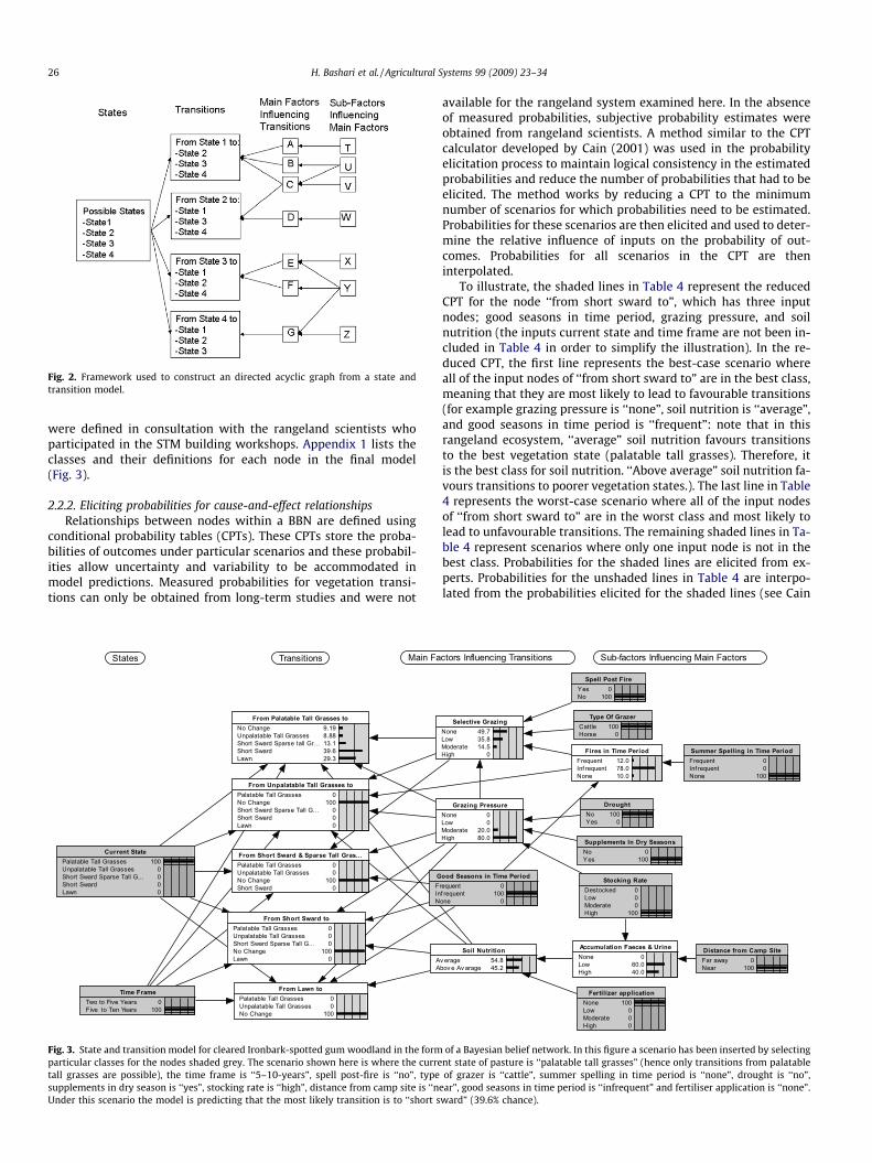
Fig. 2. Framework used to construct an directed acyclic graph from a state andtransition model.

26 H. Bashari et al. / Agricultural Systems 99 (2009) 23–34

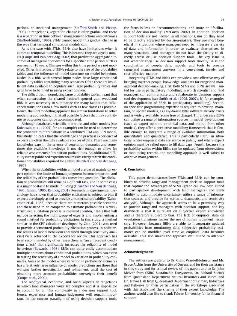
were defined in consultation with the rangeland scientists whoparticipated in the STM building workshops. Appendix 1 lists theclasses and their definitions for each node in the final model(Fig. 3).

2.2.2. Eliciting probabilities for cause-and-effect relationshipsRelationships between nodes within a BBN are defined using

conditional probability tables (CPTs). These CPTs store the proba-bilities of outcomes under particular scenarios and these probabil-ities allow uncertainty and variability to be accommodated inmodel predictions. Measured probabilities for vegetation transi-tions can only be obtained from long-term studies and were not

Fig. 3. State and transition model for cleared Ironbark-spotted gum woodland in the formparticular classes for the nodes shaded grey. The scenario shown here is where the curretall grasses are possible), the time frame is ‘‘5–10-years”, spell post-fire is ‘‘no”, typesupplements in dry season is ‘‘yes”, stocking rate is ‘‘high”, distance from camp site is ‘‘nUnder this scenario the model is predicting that the most likely transition is to ‘‘short s

available for the rangeland system examined here. In the absenceof measured probabilities, subjective probability estimates wereobtained from rangeland scientists. A method similar to the CPTcalculator developed by Cain (2001) was used in the probabilityelicitation process to maintain logical consistency in the estimatedprobabilities and reduce the number of probabilities that had to beelicited. The method works by reducing a CPT to the minimumnumber of scenarios for which probabilities need to be estimated.Probabilities for these scenarios are then elicited and used to deter-mine the relative influence of inputs on the probability of out-comes. Probabilities for all scenarios in the CPT are theninterpolated.

To illustrate, the shaded lines in Table 4 represent the reducedCPT for the node ‘‘from short sward to”, which has three inputnodes; good seasons in time period, grazing pressure, and soilnutrition (the inputs current state and time frame are not been in-cluded in Table 4 in order to simplify the illustration). In the re-duced CPT, the first line represents the best-case scenario whereall of the input nodes of ‘‘from short sward to” are in the best class,meaning that they are most likely to lead to favourable transitions(for example grazing pressure is ‘‘none”, soil nutrition is ‘‘average”,and good seasons in time period is ‘‘frequent”: note that in thisrangeland ecosystem, ‘‘average” soil nutrition favours transitionsto the best vegetation state (palatable tall grasses). Therefore, itis the best class for soil nutrition. ‘‘Above average” soil nutrition fa-vours transitions to poorer vegetation states.). The last line in Table4 represents the worst-case scenario where all of the input nodesof ‘‘from short sward to” are in the worst class and most likely tolead to unfavourable transitions. The remaining shaded lines in Ta-ble 4 represent scenarios where only one input node is not in thebest class. Probabilities for the shaded lines are elicited from ex-perts. Probabilities for the unshaded lines in Table 4 are interpo-lated from the probabilities elicited for the shaded lines (see Cain

of a Bayesian belief network. In this figure a scenario has been inserted by selectingnt state of pasture is ‘‘palatable tall grasses” (hence only transitions from palatableof grazer is ‘‘cattle”, summer spelling in time period is ‘‘none”, drought is ‘‘no”,

ear”, good seasons in time period is ‘‘infrequent” and fertiliser application is ‘‘none”.ward” (39.6% chance).

Table 4Conditional probability table for the node ‘‘from short sward to”

Factors influencing transitions from the

state “Short Sward” to another state Probability of transition to another state (%)

Grazing

pressure

Soil nutrition Good season in

time period

Palatable tall

grasses

Unpalatable tall

grasses

Short sward

sparse tall grasses

No

change

Lawn

None Average Frequent 25 25 50 0 0

None Above average Frequent 10 10 10 60 10

None Average Infrequent 10 10 30 50 0

None Above average Infrequent 0 0 15 70 15

None Average None 0 0 20 80 0

None Above average None 0 0 0 80 20

Low Average Frequent 25 25 50 0 0

Low Above average Frequent 10 10 10 55 15

Low Average Infrequent 5 5 10 80 0

Low Above average Infrequent 0 0 0 80 20

Low Average None 0 0 0 100 0

Low Above average None 0 0 0 80 20

Moderate Average Frequent 0 25 50 25 0

Moderate Above average Frequent 0 0 30 50 20

Moderate Average Infrequent 0 20 40 40 0

Moderate Above average Infrequent 0 0 35 40 25

Moderate Average None 0 0 20 80 0

Moderate Above average None 0 0 0 70 30

High Average Frequent 0 0 0 100 0

High Above average Frequent 0 0 0 70 30

High Average Infrequent 0 0 0 100 0

High Above average Infrequent 0 0 0 65 35

High Average None 0 0 0 100 0

High Above average None 0 0 0 50 50

The shaded lines represent scenarios for which probabilities estimates were elicited from rangeland scientists. Probabilities for unshaded lines were interpolated.

H. Bashari et al. / Agricultural Systems 99 (2009) 23–34 27

(2001) for a detailed explanation of the algorithm used in the inter-polation process).

2.3. Testing model behaviour

To test the behaviour of the completed BBN and identify anyinconsistencies, a sensitivity analysis was performed and the re-sults presented back for review to the rangeland scientists whohad participated previously in the STM building and the probabil-ity elicitation process. The sensitivity analysis was performed oneach transition node in the BBN by systematically selecting differ-

ent classes of their input nodes and recording the effect that thishad on the probability of transitions. For example, the differentclasses of ‘‘grazing pressure” were selected to test the influencethat this had on the transition probabilities in the node ‘‘from shortsward to” other vegetation states. When grazing pressure was setto ‘‘none”, the most likely transition was no change from the cur-rent short sward state (46.7% probability) and the second mostlikely transition was to short sward with sparse tall grasses(20.4% probability). Setting grazing pressure to ‘‘high” increasedthe probability of no change to 75%, with a 25% chance that a tran-sition to lawn would occur. This behaviour indicates that changing

Table 5Sensitivity analysis for transition ‘‘from short sward to lawn”

Rank Input node Probability (%) oftransition to lawn

Difference(% Probability)

1 Soil nutritionAverage 0 28.5Above average 28.5

2 Grazing pressureNone 7.08 17.92Low 10.8Moderate 14.2High 25

3 Good seasons in time periodFrequent 11.6 7.5Infrequent 12.2None 19.1

Input nodes are ranked from most (1) to least (3) influential on the transition.

28 H. Bashari et al. / Agricultural Systems 99 (2009) 23–34

grazing pressure causes major changes in transition probabilitiesaway from a short sward state.

Table 6Summary of sensitivity analysis performed on the transition nodes in the cleared Ironbark

Transition

Palatable tall grasses to: Unpalatable tall grasses

Short sward & sparse tall grass

Short sward

Lawn

Unpalatable tall grasses to: Palatable tall grasses

Short sward & sparse tall grass

Short sward

Lawn

Short sward & sparse tall grass to: Palatable tall grasses

Unpalatable tall grasses

Short sward

Short sward to: Palatable tall grasses

Unpalatable tall grasses

Short sward & sparse tall grass

Lawn

Lawn to: Palatable tall grasses

Unpalatable tall grasses

The shading indicates the relative influence of factors on each transition, from most influinfluence on the transition.

The results of sensitivity analysis on each transition were sum-marized into tables similar to Table 5. These tables highlight therelative influence of input nodes on transitions by showing theoverall difference in the probability of a transition caused bychanging the classes of input nodes (this difference is shown inthe difference column in Table 5). Where the results of the sensi-tivity analysis did not match the expectations of the rangelandscientists (these expectations had been recorded during thedevelopment of the STM where the expected relative influence ofeach main factor on each transition was recorded, see Table 1),the appropriate CPT was adjusted and the sensitivity analysiswas performed again.

Table 6 summarizes the results of the final sensitivity analysisfor all transitions in the Ironbark-spotted gum woodland BBN(Fig. 3). The sensitivity analysis revealed that selective grazing,grazing pressure, and soil nutrition were believed to influencemost transitions, while the fire frequency and the frequency ofgood wet seasons were also important in some transitions. Graz-ing pressure was the main driver of 12 transitions, and selective

-spotted gum woodland BBN

Selective

Grazing

Grazing

Pressure

Soil

Nutrition

Fire in

Time

Period

Good

seasons

in Time

Period

× ×

× ×

× ×

× ×

×

×

×

×

× ×

× ×

× ×

× ×

× ×

× ×

× ×

× ×

× ×

ential (black) to least influential (white). A cross (�) means that this factor had no

H. Bashari et al. / Agricultural Systems 99 (2009) 23–34 29

grazing was the main driver of three transitions. Grazing pressurewas either the most or the second most important driver of alltransitions. Selective grazing was a relatively important driver oftransitions to or from unpalatable tall grasses but had no influ-ence on transitions from short sward and lawns to tall grassstates.

Soil nutrition was relatively important for transitions to or fromlawns but had little to no influence on other transitions. Fire fre-quency had an affect on some transitions but only through its af-fect on selective grazing. Low fire frequency increased thelikelihood of selective grazing, making transitions to unpalatabletall grasses more likely. This is because, frequent fires tend tohomogenise the palatability of pastures, and so low fire frequencyleads to a diversity of palatability in pasture, leading to selectivegrazing. Frequent good seasons were important for transitionsfrom short sward and lawn states to tall grass states.

AA

Grazing Pressure

NoneLowModerateHigh

0 0

20.080.0

A

NLH

Selective Grazing

NoneLowModerateHigh

54.132.513.3 0

DestLowModeHigh

Drought

NoYes

0 100

Supplements In Dry Seasons

NoYes

100 0

From Palatable Tall Grasses t

No ChangeUnpalatable Tall GrassesShort Sward Sparse tall Gr...Short SwardLawn

9.678.198.1910.263.7

Fig. 4. Using the Bayesian belief network for predictio

From Unpalatable Tall Grasse

Palatable Tall GrassesNo ChangesShort Sward Sparse tall gr...Short SwardLawn

100 0 0 0 0

CH

Spell Post Fire

YesNo

50.749.3

Summer Spelling in T ime Period

FrequentInfrequentNone

36.533.530.0

Selective Grazing

NoneLowModerateHigh

71.214.010.44.48

Fire s in T ime Period

FrequentInfrequentNone

57.225.317.5

Good S easons in T ime Period

FrequentInfrequentNone

52.128.619.3

Fig. 5. Using the Bayesian belief network for diagnosi

2.4. Using a combined STM and BBN model for rangeland managementdecision support

A combined STM and BBN model has the ability to providerangeland managers with decision support through its analyticcapabilities. The three main types of analysis that can be per-formed are prediction, diagnosis, and sensitivity analysis. Sensitiv-ity analysis was described in Section 2.3 so examples of predictiveand diagnostic analysis are given here.

Predictive analysis can be used to answer ‘what if’ questions byselecting classes for inputs and using the model to predict theprobability of transitions, as shown in Fig. 4. In the example, the se-lected classes of input nodes represent a ‘what if’ scenario for a siteand the model predicts that the chance of transition away frompalatable tall grass to lawn is relatively high (64%) within a5–10-year timeframe (note that the class ‘5–10-years’ is selected

Soil Nutrition

veragebove Avarage

5.0095.0

ccumulation Faeces & Urine

oneowigh

0 0

100

Fertilizer application

NoneLowModerateHigh

100 0 0 0

Distance from Camp Site

Far awayNear

0 100

Stocking Rate

ocked

rate

0 0 0

100

o

Time Frame

Two to five yearsFive to Ten years

0 100

n (shaded nodes represent the selected scenario).

s to

Time Frame

Two to five yearsFive to Ten years

0 100

Type Of Grazer

attleorse

50.349.7

Grazing Pressure

NoneLowModerateHigh

71.211.517.4 0

Stocking Rate

DestockedLowModerateHigh

71.217.69.781.47

Supple ments In Dry Seasons

NoYes

51.548.5

Drought

NoYes

54.245.8

s (shaded nodes represent the selected scenario).

30 H. Bashari et al. / Agricultural Systems 99 (2009) 23–34

in the time frame node). The model also indicates the probablecauses for this transition:high grazing pressure (80% chance) andabove-average soil nutrition (95% chance).

Diagnostic analysis can be used to answer ‘how’ questions byselecting a desired outcome and using the model to identify thescenario that is most likely to lead to that outcome, as shown inFig. 5. In this example, the model is used to identify how a landmanager might shift pasture from an unpalatable tall grass stateto a palatable tall grass state within a 5–10-year time frame (notethat the class ‘5–10-years’ is selected in the time frame node). Themodel shows that this transition is most likely if grazing pressureand selective grazing are absent (see the selective grazing andgrazing pressure nodes), and this is most likely where destockingis applied (see the stocking rate node). The model also shows thatfrequent fires are important for achieving low to no selective graz-ing (see the fires in time period node), and in turn, good seasonsare important for achieving frequent fires (see the good seasonsin time period node).

3. Discussion

3.1. Pasture dynamics in cleared Ironbark-spotted gum woodland

The combined STM and BBN model developed in this paper re-vealed that grazing pressure is the main factor driving almost allpasture transitions in the cleared Ironbark-spotted gum woodlandecosystem studied. Stocking rate had the greatest influence ongrazing pressure, but drought and the use of dry-season supple-ments magnified the influence of stocking rate. This finding is sup-ported by Walker (1995), who also suggested that stocking rate isthe most important variable in grazing management. If the stockingrate is not in balance with available forage, regardless of other graz-ing management practices (timing, distribution, and type of live-stock), grazing management objectives will probably not be met.

Selective grazing was highlighted by the model as an importantfactor in transitions from or to unpalatable tall grasses. It is one ofthe key factors influencing the vegetation composition in grasslands(Ksiksi et al., 2005) and covers items such as diet selection, land-scape selection, and bite selection (Senft et al., 1987). Selective graz-ing has a significant effect on the competitive interactions of plantsand the structure and function of ecosystems (Archer and Smeins,1991; Belsky, 1992) as it creates gaps in the pasture, allowing unpal-atable tall grasses such as Aristida sp. and Bothriochloa deciepiens toestablish. Drought can accelerate this gap creation because it re-duces the seed set of favourable grasses such as H. contortus, whichcan also accelerate the establishment of exotic pasture species (Ashand Ksiksi, 1999). Selective grazing can be reduced using frequentfire to homogenise the palatability of pasture and spelling post-fireto allow palatable species such as H. contortus to establish. Theimportance of selective grazing, as highlighted by the model, sug-gests that more research is needed to clarify the exact effect of selec-tive grazing on rangeland vegetation dynamics and its condition.

Occurrence of good seasons and bad seasons (drought) weretwo unmanageable factors that had an influence on vegetationstate via their direct impact on grazing pressure and fire frequency.This indicates that drought and climate change are likely to have abig impact on the state of rangelands, particularly where stockingrates and spelling regimes are not managed appropriately.

Soil nutrition was another environmental variable that could beaffected by grazing management. It is considered by McIvor et al.(2005) to be an important factor in transitions from any state tolawns. Land managers can adjust soil nutrition by changing thestocking rate and by locating watering points to minimize theaccumulation of faeces and urine at any one site. The implementa-tion of some form of grazing system such as rotational grazing can

help to distribute evenly the impact of animals through all parts ofa paddock (Johnston et al., 2005).

3.2. Use of the combined STM and BBN model for adaptivemanagement in rangelands

Adaptive management refers to the process of using manage-ment outcomes to continuously modify or adapt managementpractice (Janssen et al., 2000; Sabine et al., 2004; Morghan et al.,2006). It is a process of ‘‘learning by doing” whereby managementobjectives are set and management plans developed using currentknowledge of the management system (which can be in the formof a model). Actions are implemented and monitored. Monitoringresults are then used to evaluate management success and modifymanagement objectives or plans where necessary.

Adaptive management is particularly important for rangelandmanagement because rangelands are complex systems in whichthe outcomes of management decisions are often difficult to pre-dict. While the importance of adaptive management in rangelandmanagement has been stated frequently in the literature, veryfew tools to support it have been provided. Hence, rangelandmanagement tools are needed that not only capture the uncer-tainty associated with rangeland dynamics, but also supportadaptive management by being updatable using monitoring data(Ringold et al., 1996). A combined STM and BBN model has poten-tial to provide such a tool because BBNs can learn from monitor-ing data. Put simply, the probability tables within BBNs can beupdated iteratively by importing monitoring results. This is calledincorporating ‘case data’ (or data from previous cases) into themodel.

A demonstration of this model-updating process is not possi-ble here because empirical data for transitions in the rangelandecosystem studies are not available. Hypothetically, however,the process would work by monitoring the vegetation state of arangeland at many sites, and simultaneously monitoring the mainfactors and sub-factors stated in the model as influencing vegeta-tion state transitions (such as grazing pressure, fire frequency,etc.). The result of monitoring would be a record describing priorvegetation state, management actions implemented, and theoccurrence of environmental events, and any vegetation statetransitions that occurred. The model could then learn from thesedata by adjusting conditional probabilities to reflect real-wordobservations. Hence, a combined STM and BBN model could pro-vide a tool for evaluating the likely influence of previous manage-ment actions and environmental scenarios on vegetation state, aswell as a predictive tool for planning future rangeland manage-ment actions.

3.3. The modelling approach

This paper has shown how rangeland dynamics can be mod-elled by combining STMs and BBNs. It captures the advantages ofboth STMs and BBNs to provide decision support tools that (a)are simple graphical models describing rangeland vegetationchange in relation to management actions and environmentalevents (e.g. drought), (b) can be used for scenario and diagnosticanalysis to answer ‘‘what if” and ‘‘how” questions, (c) can be ap-plied in areas where empirical data are scarce by utilizing experi-ential knowledge, (d) can utilise empirical data where available,(e) can accommodate uncertainty, and (f) show promise in beingable to support adaptive management.

There are significant criticisms in the literature of both the STMand the BBN modelling approaches. STMs have been criticised forbeing ‘‘event-driven” models of vegetation dynamics (Watsonet al., 1996) in which transitions are a result of infrequent andunpredictable events such as drought, fire, favourable climatic

H. Bashari et al. / Agricultural Systems 99 (2009) 23–34 31

periods, or sustained management (Stafford-Smith and Pickup,1993). In rangelands, vegetation change is often gradual and thereis a separation in time between management actions and outcomes(Stafford-Smith, 1996). STMs cannot model this gradual change inthe way that temporal simulation models can.

As is the case with STMs, BBNs also have limitations when itcomes to temporal modelling. This is because they are acyclic mod-els (Coupe and Van der Gaag, 2002) that predict the aggregate out-comes of management or events for a specified time period, such asone year or 10 years. Changes within this time period are not mod-elled. Other limitations of BBNs relate to the size of the probabilitytables and the influence of model structure on model behaviour.Nodes in a BBN with several input nodes have large conditionalprobability tables containing many scenarios. Often there are insuf-ficient data available to populate such large probability tables andgaps have to be filled in using expert opinion.

The difficulties in populating large probability tables meant thatwhen constructing the cleared Ironbark-spotted gum woodlandBBN, it was necessary to summarize the many factors that influ-enced transitions into a few nodes with as few classes as possible.Hence, the BBN modelling approach has similar limitations to othermodelling approaches, in that all possible factors that may contrib-ute to outcomes cannot be accommodated.

Although databases, scientific literature, and other models (seeKoivusalo et al. (2005) for an example) can be used to determinethe probabilities of transitions in a combined STM and BBN model,this study indicates that the knowledge and practical experience ofexperts are often the only available sources of data. There are manyknowledge gaps in the science of vegetation dynamics and some-times the available knowledge is not rich enough to allow forreliable assessments of transition probabilities. An additional diffi-culty is that published experimental results rarely match the condi-tional probabilities required for a BBN (Druzdzel and Van der Gaag,1995).

When the probabilities within a model are based mainly on ex-pert opinion, the limits of human judgment become important andthe reliability of the probabilities comes into question. The elicita-tion of probabilities still remains a difficult task, and in some casesis a major obstacle to model building (Druzdzel and Van der Gaag,1995; Jensen, 1995; Renooij, 2001). Research in experimental psy-chology has shown that probability elicitation is subject to bias ifexperts are simply asked to provide a numerical probability (Kahn-eman et al., 1982) because there are numerous possible scenariosand these need to be compared to estimate probabilities. A well-structured elicitation process is required (Fenton, 1998) that willinclude selecting the right group of experts and implementing asound method for probability elicitation. In this study, a methodsimilar to the CPT calculator developed by Cain (2001) was usedto provide a structured probability elicitation process. In addition,the results of model behaviour (obtained through sensitivity anal-ysis) were returned to the experts for review. This approach hasbeen recommended by other researchers as ‘‘an antecedent condi-tions check” that significantly increases the reliability of modelbehaviour (Edwards, 1998). BBNs can quite easily accommodatemultiple opinions about conditional probabilities, which can assistin testing the sensitivity of a model to variation in probability esti-mates. Areas of the model where variation in probability estimateshas a relatively large influence on model predictions are those thatwarrant further investigation and refinement, until the cost ofobtaining more accurate probabilities outweighs their benefit(Coupe et al., 2000).

The biophysical, economic, and social aspects of rangelandsin which land managers work are complex and it is impossibleto account for all this complexity in a decision support tool.Hence, experience and human judgement will remain impor-tant. In the current paradigm of using decision support tools,

the focus is less on ‘‘recommendations” and more on ‘‘facilita-tion of decision-making” (McCown, 2002). In addition, decisionsupport tools are not needed in all situations, nor do they needto be directly accessed by decision-makers. They are most ben-eficial in situations where managers need to integrate a varietyof data and information in order to evaluate alternatives. Inmany situations, land managers do not have the facility to di-rectly access or use decision support tools. The key issue isnot whether they use decision support tools directly; it is thecoordination of people, data, models, and tools to providerangeland management answers in a convenient, timely, andcost-effective manner.

Integrating STMs and BBNs can provide a cost-effective way ofbringing together people, knowledge, and data for rangeland man-agement decision-making. First, both STMs and BBNs are well sui-ted for use in participatory modelling in which scientist and landmanagers can communicate and collaborate in decision supporttool development (see Smith et al. (2005, 2007a, b) for examplesof the application of BBNs in participatory modelling). Second,no specialist programming expertise is required to develop, main-tain, or update models, as easy-to-use BBN software already existsand is widely available (some free of charge). Third, because BBNscan utilise a range of information sources in model development(such as expert opinion, empirical data, and output from othermodels), they offer a predictive modelling framework that is flex-ible enough to integrate a range of available information, bothquantitative and qualitative. This is particularly useful in situa-tions where empirical data are scarce or patchy and where expertopinion must be relied upon to fill data gaps. Fourth, because theprobability tables within BBNs can be updated from observationsor monitoring records, the modelling approach is well suited toadaptive management.

4. Conclusion

This paper demonstrates how STMs and BBNs can be com-bined to develop rangeland management decision support toolsthat capture the advantages of STMs (graphical, low cost, suitedto participatory development with land managers) and BBNs(ability to accommodate uncertainty, utilise a range of informa-tion sources, and provide for scenario, diagnostic, and sensitivityanalysis). Although, the approach seems to be a promising wayto provide rangeland managers with decision support, one keydrawback is that it is reliant on subjective expert knowledgeand is therefore subject to bias. The lack of empirical data onvegetation transitions makes the use of human judgment neces-sary. However, because BBNs are able to incorporate updatedprobabilities from monitoring data, subjective probability esti-mates can be modified over time as empirical data becomesavailable. This also makes the approach well suited to adaptivemanagement.

Acknowledgments

The authors are grateful to Dr. Grant Wardell-Johnson and Mr.Bruce Alchin from the University of Queensland for their assistancein this study and for critical review of this paper; and to Dr. JohnMcIvor from CSIRO Sustainable Ecosystems, Dr. Richard Silcockfrom Queensland Department Natural Resources and Mines, andDr. Trevor Hall from Queensland Department of Primary Industriesand Fisheries for their participation in the workshops associatedwith this study and the sharing of their expert knowledge. Theauthors would also like to thank Tehran University for its financialsupport.

Appendix 1

Definitions for nodes and their classes in the cleared Ironbark-spotted gum woodland Bayesian belief network (Fig. 3)

Node Definition and classes

Current state This node represents possible vegetation states that can occur at the site of interestPalatable tall grasses: perennial palatable tall tussock grasses such as Heteropogon contortus, high soil stabilityUnpalatable tall grasses: perennial unpalatable tussock grasses such as Aristida sp. and Bothriochloa decipiens,erosion moderate to highShort sward and sparse tall grass: short grasses such as Eragrostis sororia interspersed with tall tussock grasses,erosion moderate to highShort sward: short grasses such as Eragrostis sororia, erosion moderate to lowLawn: very stable and resistant to disturbances such as grazing and trampling, includes species such as Cynadondactylon

Timeframe This node represent periods of time over which transitions may occur at the site of interest2–5-years5–10-years

From palatable tallgrasses to

This node represents transitions away from palatable tall grasses to another vegetation state at the site of interestNo change: vegetation remains in the palatable tall grass stateUnpalatable tall grasses: vegetations moves to the unpalatable tall grass stateShort sward and sparse tall grass: vegetations moves to the short sward and sparse tall grass stateShort sward: vegetations moves to the short sward stateLawn: vegetations moves to the lawn state

From unpalatable tallgrasses to

This node represents transitions away from unpalatable tall grasses to another vegetation state at the site ofinterestPalatable tall grasses: vegetations moves to the palatable tall grass stateNo change: vegetation remains in the unpalatable tall grass stateShort sward and sparse tall grass: vegetations moves to the short sward and sparse tall grass stateShort sward: vegetations moves to the short sward stateLawn: vegetations moves to the lawn state

From short sward andsparse tall grassesto

This node represents transitions away from short sward and sparse tall grasses to another vegetation state at thesite of interestPalatable tall grasses: vegetations moves to the palatable tall grass stateUnpalatable tall grasses: vegetations moves to the unpalatable tall grass stateNo change: vegetation remains in the short sward and sparse tall grass stateShort Sward: vegetations moves to the short sward state

From short sward to This node represents transitions away from short sward to another vegetation state at the site of interestPalatable tall grasses: vegetations moves to the palatable tall grass stateUnpalatable tall grasses: vegetations moves to the unpalatable tall grass stateShort sward and sparse tall grass: vegetations moves to the short sward and sparse tall grass stateNo change: vegetation remains in the short sward stateLawn: vegetations moves to the lawn state

From lawn to This node represents transitions away from lawn to another vegetation state at the site of interestPalatable tall grasses: vegetations moves to the palatable tall grass stateUnpalatable tall grasses: moves to the unpalatable tall grass stateNo change: vegetation remains in the lawn state

Selective grazing This node represents the selectivity of grazing at the site of interest. Selective grazing mostly occurs in largecontinuously grazed pastures where stock preferentially eat the most palatable speciesNone: plant composition is consistent and uniform and contains palatable species (this situation is rare)Low: there are many uniform palatable species available in the pasture but some unpalatable ones are presentModerate: palatable species are patchy in the pastureHigh: palatable species are rare and hidden among unpalatable species in the pasture

Grazing pressure This node represents the balance between how much grazing animals eat and how fast the pasture grows at thesite of interest (grazing pressure = rate of removal of pasture/rate of supply of pasture)None: grazing pressure of 0Low: supply of pasture is much more than the rate of removal of pasture (grazing pressure �1)Moderate: supply of pasture is more than the rate of removal of pasture (grazing pressure <1)High: supply of pasture is equal to or less than the rate of removal of pasture (grazing pressure P1)

Soil nutrition This node represents the soil nutritional status at the site of interest. In the case study area, above average soilnutrition had an effect on transitions to lawn state so there are two states for soil nutrition, average and aboveaverage. Below average soil nutrition was not considered to be an important factor in any transitions in the casestudy area. Therefore this class of soil nutrition was not included in the modelAverage: 50–200 kg N per ha per annumAbove average: more than 200 kg N per ha per annum

(continued on next page)

32 H. Bashari et al. / Agricultural Systems 99 (2009) 23–34

Appendix 1 (continued)

Node Definition and classes

Fertiliser application This node represents the level of fertiliser application at the site of interest (fertiliser = 10% nitrogen, 3.4%phosphorus, 6.4% potassium)None: no fertiliserLow: less than 50 kg N per annum plus other nutrientsModerate: 50–150 kg N per ha per annum plus other nutrientsHigh: more than 150 kg N per ha per annum plus other nutrients

Accumulation faecesand urine

This node represents the level of faeces and urine accumulation caused by cattle at the site of interestNone: there is no faeces and urine from stock in the pastureLow: the accumulation of faeces and urine exists in the pasture but it is not considerable (<3% of the soil cover)High: there is a considerable amount of faeces and urine in the pasture (>3% of the soil cover)

Distance fromcampsite

This node represents the distance of the site of interest from a campsite, which is a site where cattle congregate.Campsites are usually watering pointsFar away: more than 500 m from a campsiteNear: less than 500 m from a campsite

Stocking rate This node represents the number of hectares per beastDestocked: no stock presentLow: 1 beast per 6–8 haModerate: 1 beast per 4–6 haHigh: more than 1 beast per 4 ha

Supplement in dryseason

This node classes whether or not cattle are fed supplements in the dry season. Supplementary feeding tends toallow land managers to maintain cattle numbers in dry timesNo: no feed supplements fed in the dry seasonYes:feed supplements fed in the dry season

Drought This node classes whether or not drought is present at the site of interest. Drought occurs when rainfall lies abovethe lowest five per cent of recorded rainfall but below the lowest 10 percent for the period in questionNo: drought is absentYes: drought is present

Good seasons in timeperiod

This node represents the frequency of good seasons at the site of interest within the time period of interest. Agood season is defined as a wet season with more that average rainfall.Frequent: 3 of 5 years or 7 of 10 years with more than average rainfallInfrequent: 1–2 of 5 years or 1–6 of 10 years with more than average rainfallNone: no years with more than average rainfall in the time period

Fires in time period This node represents the frequency of fires at the site of interest within the time period of interestFrequent: fire occurs in 3 of 5 years or 7 of 10 yearsInfrequent: fire occurs 1–2 of 5 years or 1–6 of 10 yearsNone: fire occurs 0 of 5 years or 0 of 10 years

Type of grazer This node represents the type of animal grazing at the site of interestCattleHorse

Post-fire spelling This node classes whether or not the pasture at the site of interest is spelt for at least 10 days after burning or untilthe grass is 10 cm high:Yes: post-fire spelling occursNo: post-fire spelling does not occur

Summer spelling intime period

This node represents the frequency of summer spelling of pasture at the site of interest within the time period ofinterestFrequent: pasture spelled in 3 of 5 years or 7 of 10 yearsInfrequent: pasture spelled 1–2 of 5 years or 1–6 of 10 yearsNone: pasture spelled 0 of 5 years or 0 of 10 years

H. Bashari et al. / Agricultural Systems 99 (2009) 23–34 33

References

Allen-Diaz, B., Bartolome, J.W., 1998. Sage brush-grass vegetation dynamics:comparing classical and state transition model. Ecological Application 8, 795–804.

Archer, S., Smeins, F.E., 1991. Ecosystem-level processes. In: Heitschmidt, R.K. et al.(Eds.), Grazing Management an Ecological Perspective. Timber Press Inc.,Portland, Ore, pp. 109–139.

Ash, A.J., Ksiksi, T., 1999. Managing woodland: developing sustainable beefproduction systems for northern Australia. In: Lambert, J. (Ed.), Peer Reviewof Resource and Whole Property Management Projects. Northern AustraliaProgram Occasional Publication No. 10, Genstat, pp. 1–7.

Belsky, J.A., 1992. Effects of grazing composition, disturbance and fire on speciescomposition and diversity in grassland communities. Vegetation Science 3,187–200.

Cain, J., 2001. Planning Improvements in Natural Resources Management.Guidelines for Bayesian Networks to Support the Planning and Management

of Development Programmes in the Water Sector beyond. Centre for Ecologyand Hydrology, Wallingford, UK.

Cain, J.D., Jinapala, K., Makin, I., Somaratna, P.G., Ariyarantna, B.R., Perera, L.R., 2003.Participatory decision support for agriculture management. A case study fromSri Lanka. Agricultural Systems 76, 457–482.

Coupe, V.M.H., Van Der Gaag, L.C., 2002. Properties of sensitivity analysis ofBayesian belief networks. Annuals of Mathematics and Artificial Intelligence 36,323–356.

Coupe, V.M.H., Van Der Gaag, L.C., Habbema, J.D.F., 2000. Properties of sensitivityanalysis of Bayesian belief networks. The Knowledge Engineering Review 15,215–232.

Druzdzel, M.J., Van Der Gaag, L.C., 1995. Elicitation of probabilities for beliefnetworks: combining qualitative and quantitative information. In: Calif, M.P.(Eds.), Proceedings of the 11th Conference on Uncertainty in ArtificialIntelligence. pp. 141–148.

Edwards, W., 1998. Hailfinder tools for and experiences with Bayesian normativemodeling. American Psychologist 53, 416–428.

34 H. Bashari et al. / Agricultural Systems 99 (2009) 23–34

Fenton, N., 1998. Probability Elicitation and Bias. Available from: <http://www.dcs.qmul.ac.uk/~norman/BBNs/BBNs.htm>.

Friedel, M., 1991. Range condition assessment and the concept of thresholds: aviewpoint. Journal of Range Management 44, 422–426.

Hall, T.J., Filet, P.G., Banks, B., Silcock, R.G., 1994. A state and transition model of theAristida–Bothriochloa pasture community of central and southern Queensland.Tropical Grassland 28, 270–273.

Henriksen, H.J., Barlebo, H.C., 2008. Reflections on the use of Bayesian networks foradaptive management. Journal of Environmental Management. 88, 1025–1036.

Janssen, M.A., Walker, B.H., Langridge, J., Abel, N., 2000. An adaptive agent model foranalyzing co-evaluation of management and policies in a complex rangelandsystem. Ecological Modelling 131, 249–268.

Jensen, A.L., 1995. Quantification experience of a DSS for mildew management inwinter wheat. In: Druzdzel, M.J. et al. (Eds.), Working Notes of the IJCAIWorkshop on Building Probabilistic Networks: Where do the Numbers ComeFrom? American Association for Artificial Intelligence, pp. 23–31.

Jensen, F.V., 1996. An Introduction to Bayesian Networks. University College LondonPress.

Jensen, F.V., 2001. Bayesian Networks and Decision Graphs. Springer, New York.Johnston, W.H., Cornish, P.S., Koen, T.B., Shoemark, V.F., 2005. Eragrostis curvula

(Schrad.) Nees. complex pastures in southern New South Wales, Australia: acomparison of Eragrostis curvula cv. Consol and Medicago sativa L. cv. Novaunder intensive rotational management. Australian Journal of ExperimentalAgriculture 45, 1255–1266.

Kahneman, D., Slovic, P., Tversky, A., 1982. Judgement Under Uncertainty:Heuristics and Biases. Cambridge University Press.

Koivusalo, H., Kokkonen, T. Laine, H.A. Jolma, o. Varis., 2005. Exploiting simulationmodel results in parameterising a Bayesian network – a case study of dissolvedorganic carbon in catchment runoff. In: Zerger, A., Argent, R.M., (Eds.),Proceedings of the MODSIM International Congress on Modelling andSimulation. Modelling and Simulation Society of Australia and New Zealand,pp. 421–427.

Ksiksi, T., Ash, A., Corfield, J., 2005. Assessing a simple technique to predict forageselection by cattle grazing northern Queensland rangelands. Arid Land Researchand Management 19, 363–372.

Laycock, W.A., 1991. Stable states and thresholds of range condition on NorthAmerican rangeland: a view point. Journal of Range Management 44, 427–433.

Ludwig, J., Tongway, D., Frreudenberger, D., Noble, J., Hodgkinson, K., 1996.Landscape Ecology Function and Management: Principles from Australia’sRangelands. CSIRO Publishing, Australia.

Lynam, T., 2001. Participatory Systems Analysis: An Introductory Guide. Institute ofEnvironmental Studies Special Report. University of Zimbabwe, Harare,Zimbabwe.

Matthews, K.B., Schwarz, G., Buchan, K., Rivington, M., 2005. Wither agriculturalDSS? In: Zerger, A., Argent, R.M. (Eds.), MODSIM International Congress onModelling and Simulation, Modelling and Simulation Society of Australia andNew Zealand, pp. 224–231.

McCann, R.K., Marcot, B.G., Ellis, R., 2006. Bayesian belief networks: applications inecology and natural resource management. Canadian Journal of Forest Research36, 3053–3062.

McCown, R.L., 2002. Changing systems for supporting farmers’ decisions: problems,paradigms, and prospects. Agricultural Systems 74, 179–220.

McIvor, J.G., Mcintyre, S., Saeli, I., Hodgkinson, J.J., 2005. Patch dynamics in grazedsubtropical native pastures in south-east Queensland. Austral Ecology 30, 445–464.

Morghan, K.J.R., Sheley, R.l., Svejcar, T.J., 2006. Successful adaptive management –the integration of research and management. Rangeland Ecology andManagement 59, 216–219.

National Land and Water Resources Audit, 2004. National Resources Models in theRangelands, a Review Undertaken for National Land and Water Resources Audit,Sustainable Ecosystems. CSIRO, Brisbane.

Nyberg, J.B., Marcot, B.G., Sulyma, R., 2006. Using Bayesian belief networksin adaptive management. Canadian Journal of Forest Research 36, 3104–3116.

Orr, D.M., Paton, C.J., McIntyre, S., 1994. A state and transition model for thesouthern black spear grass zone of Queensland. Tropical Grassland 28,266–269.

Phelps, D.G., Bosch, O.J.H., 2002. A quantitative state and transition model for theMitchell grassland of central western Queensland. Rangeland Journal 24, 242–267.

Pilke Jr., R.A., 2001. Room for doubt. Nature 410, 151–152.Pilke Jr., R.A., 2003. The role of models in prediction for decision. In: Canham, C.D.

et al. (Eds.), Model in Ecosystem Science. Princeton University Press, NewJersey.

Prato, T., 2005. Bayesian adaptive management of ecosystems. Ecological Modelling138, 147–156.

Raymond, A.E., Love, R.M., 1957. The step-point method of sampling – a practicaltool in range research. Journal of Range Management 10, 208–212.

Renooij, S., 2001. Probability elicitation for belief networks: issues to consider. TheKnowledge Engineering Review 16, 255–269.

Ringold, P.L., Alegaria, J., Czaplewski, R.L., Mulder, B.S., Tolie, T., Burnett, K., 1996.Adaptive monitoring design for ecosystem management. Ecological Application6, 745–747.

Sabine, E., Schreiber, G., Bearlin, A.R., Nicol, S.J., Todd, C.R., 2004. Adaptivemanagement: a synthesis of current understanding and effective application.Ecological Management and Restoration 5, 177–182.

Senft, R.L., Coughenour, M.B., Bailey, D.W., Rittenhouse, L.R., Sala, O.E., 1987. Largeherbivore foraging and ecological hierarchies. Bioscience 37, 759–799.

Smith, C.S., Russell, I., King, C., 2005. Rats and rice: belief network models ofrodent control in the rice field of Cambodia. In: Zerger, A., Argent, R.M. (Eds.),MODSIM 2005 International Congress on Modelling and Simulation.Modelling and Simulation Society of Australia and New Zealand, pp. 449–455.

Smith, C.S., Felderhof, L., Bosch, O.J.H., 2007a. Adaptive management: making ithappen through participatory systems analysis. Systems Research andBehavioral Science 24, 567–587.

Smith, C.S., Howes, A.L., Price, B., McAlpine, C.A., 2007b. Using a Bayesian beliefnetwork to predict suitable habitat of an endangered mammal – the Julia Creekdunnart (Sminthopsis douglasi). Biological Conservation 139, 333–347.

Stafford-Smith, D.M., 1996. Management of rangeland paradigms at their limits. In:Hodgson, J.G. et al. (Eds.), The Ecology and Management of Grazing Systems.CAB International, Wallingfold, UK, pp. 325–357.

Stafford-Smith, D.M., Pickup, G., 1993. Out of Africa, looking in understandingvegetation change. In: Behanke, R.H. et al. (Eds.), Range Ecology atDisequilibrium. Overseas Development Institute, London, pp. 196–226.

Tongway, D., Hindley, N.L., 2004. Landscape Function Analysis: Procedures forMonitoring and Assessing Landscape, Sustainable Ecosystems. CSIRO, Brisbane.

Tothill, J.C., Gillies, C.C., 1992. The Pasture Lands of Northern Australia: TheirCondition Productivity and Sustainability. Occasional Publication, TropicalGrassland of Australia.

Uusitalo, L., 2007. Advantages and challenges of Bayesian networks inenvironmental modelling. Ecological Modelling 203, 312–318.

Walker, J.W., 1995. Viewpoint: grazing management and research now and in thenext millennium. Journal of Range Management 48, 350–357.

Watson, I.W., Burnside, D.G., Holm, A.M., 1996. Event-driven or continuous; whichis the better model for managers? Rangeland Journal 18, 351–369.