developing mapreduce programs
TRANSCRIPT

Developing MapReduce Programs
Dell Zhang
Birkbeck, University of London
2018/19
Cloud Computing
MapReduce Algorithm Design

MapReduce: Recap
• Programmers must specify two functions:map (k, v) → <k’, v’>*
• Takes a key value pair and outputs a set of key value pairs, e.g., key= filename, value= a single line in the file
• There is one Map call for every (k,v) pair
reduce (k’, <v’>*) → <k’, v’’>*• All values v’ with same key k’ are reduced together and
processed in v’ order
• There is one Reduce function call per unique key k’

MapReduce: Recap
• Optionally, programmers also specify:combine (k’, v’) → <k’, v’>*
• Mini-reducers that run in memory after the map phase
• Used as an optimization to reduce network traffic
partition (k’, #partitions) → partition for k’• Often a simple hash of the key, e.g., hash(k’) mod n
• Divides up key space for parallel reduce operations
MapReduce: Recap
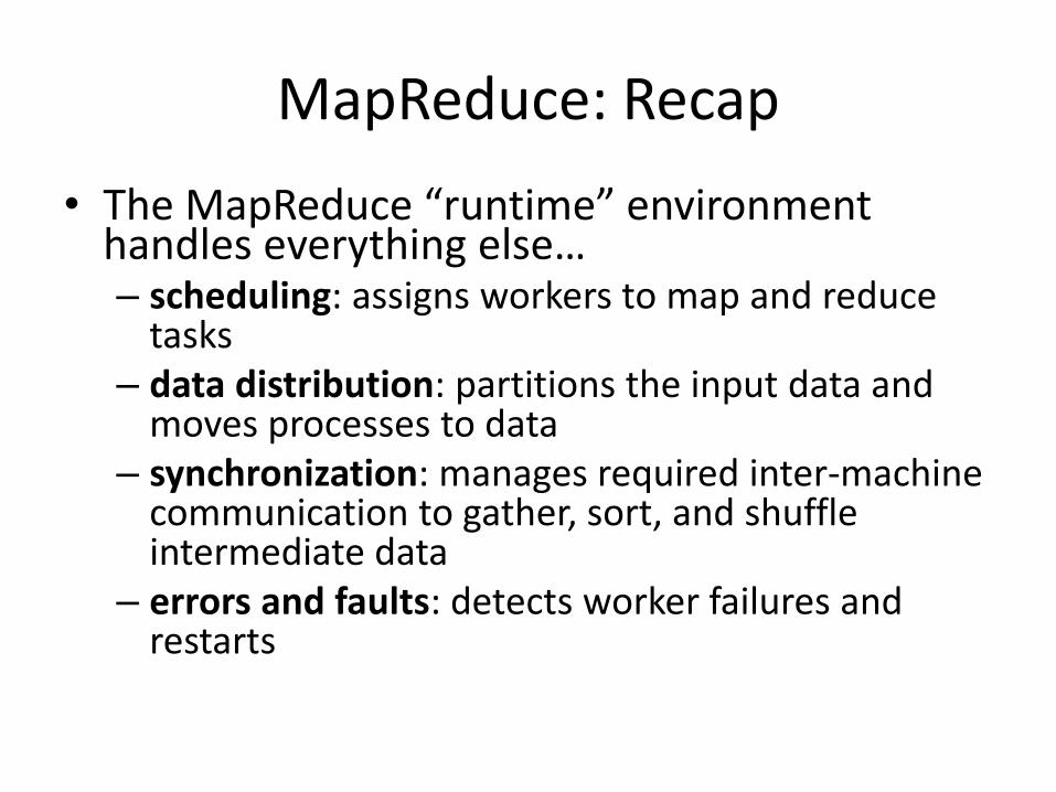
• The MapReduce “runtime” environment handles everything else…– scheduling: assigns workers to map and reduce
tasks– data distribution: partitions the input data and
moves processes to data– synchronization: manages required inter-machine
communication to gather, sort, and shuffle intermediate data
– errors and faults: detects worker failures and restarts

MapReduce: Recap
• You have limited control over data and execution flow– All algorithms must expressed in m, r, c, p
• You don’t (need to) know:– Where mappers and reducers run
– When a mapper or reducer begins or finishes
– Which input a particular mapper is processing
– Which intermediate key a particular reducer is processing


Tools for Synchronization
• Cleverly-constructed data structures– Bring partial results together
• Sort order of intermediate keys– Control the order in which reducers process keys
• Partitioner– Control which reducer processes which keys
• Preserving state in mappers and reducers– Capture dependencies across multiple keys and
values
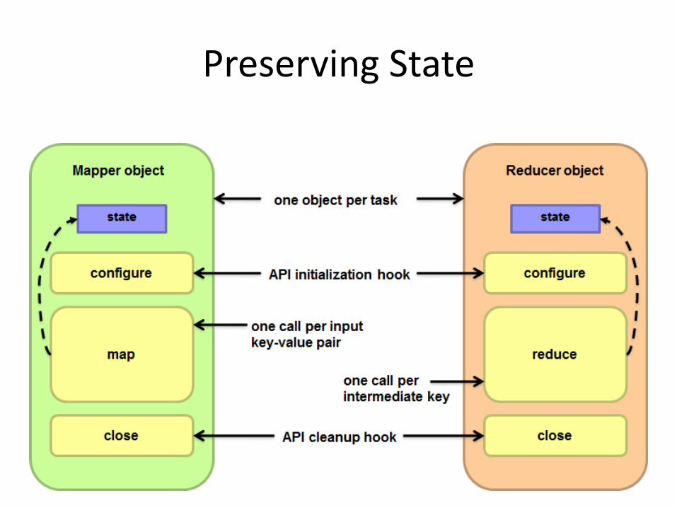
Preserving State
Scalable Hadoop Algorithms: Themes
• Avoid object creation
– Inherently costly operation
– Garbage collection
• Avoid buffering
– Limited heap size
– Works for small datasets, but won’t scale!

Importance of Local Aggregation
• Ideal scaling characteristics:– Twice the data, twice the running time
– Twice the resources, half the running time
• Why can’t we achieve this?– Synchronization requires communication
– Communication kills performance
• Thus… avoid communication!– Reduce intermediate data via local aggregation
– Combiners can help

Word Count: Baseline
What’s the impact of combiners?
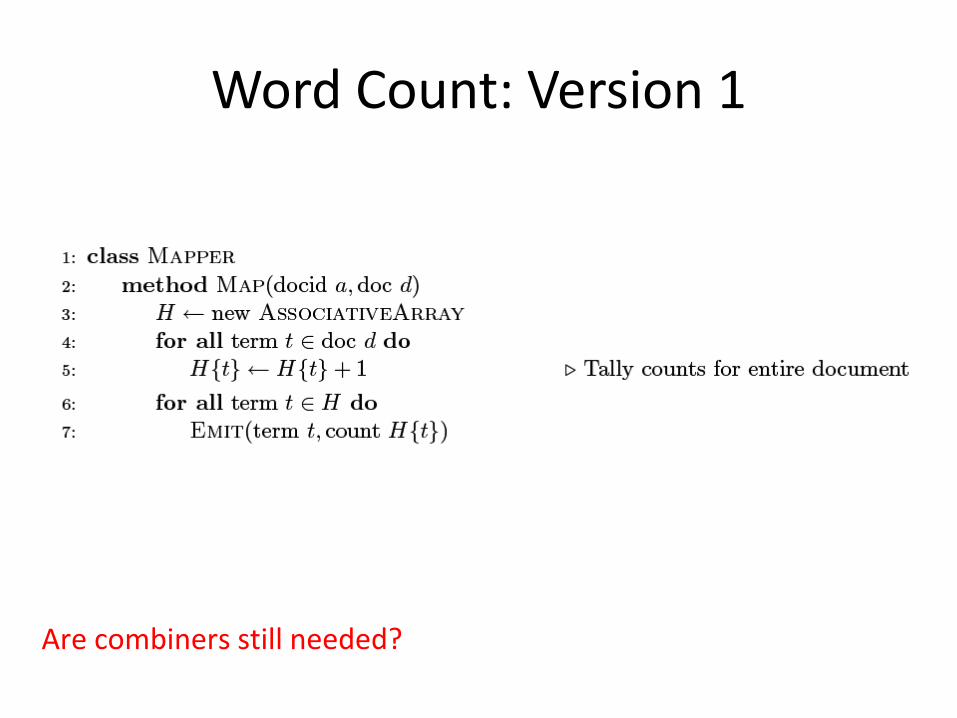
Word Count: Version 1
Are combiners still needed?
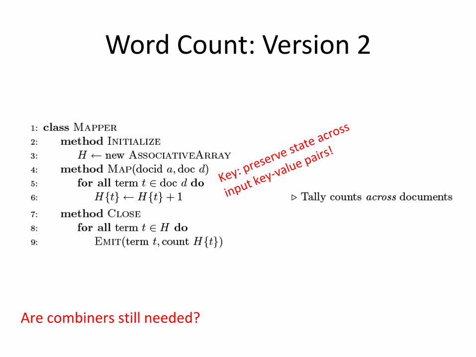
Word Count: Version 2
Are combiners still needed?

Design Pattern for Local Aggregation
• “In-mapper combining”
– Fold the functionality of the combiner into the mapper by preserving state across multiple map calls
• Advantages
– Speed
– Why is this faster than actual combiners?
• Disadvantages
– Explicit memory management required
– Potential for order-dependent bugs

Combiner Design
• Combiners and reducers share same method signature
– Sometimes, reducers can serve as combiners
– Often, not…
• Remember: combiner are optional optimizations
– Should not affect algorithm correctness
– May be run 0, 1, or multiple times
• Example: find average of all integers associated with the same key
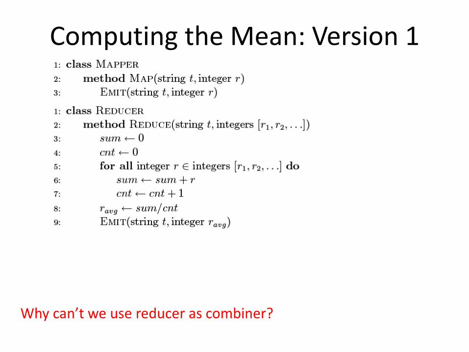
Computing the Mean: Version 1
Why can’t we use reducer as combiner?
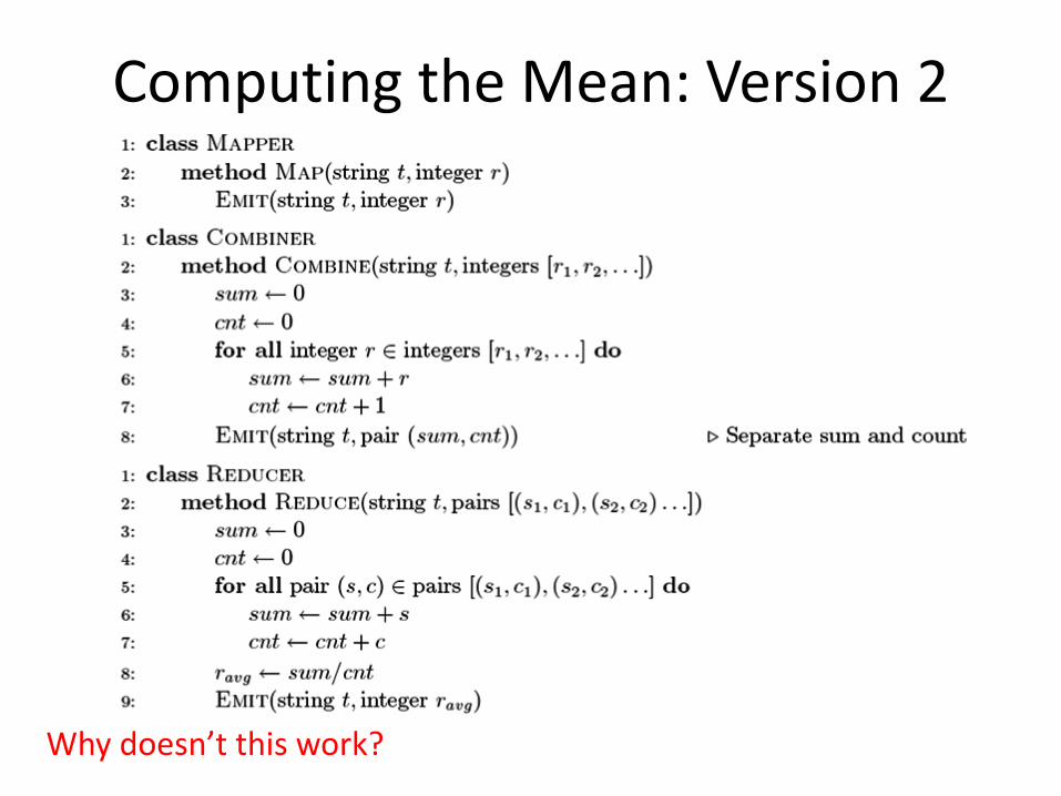
Computing the Mean: Version 2
Why doesn’t this work?
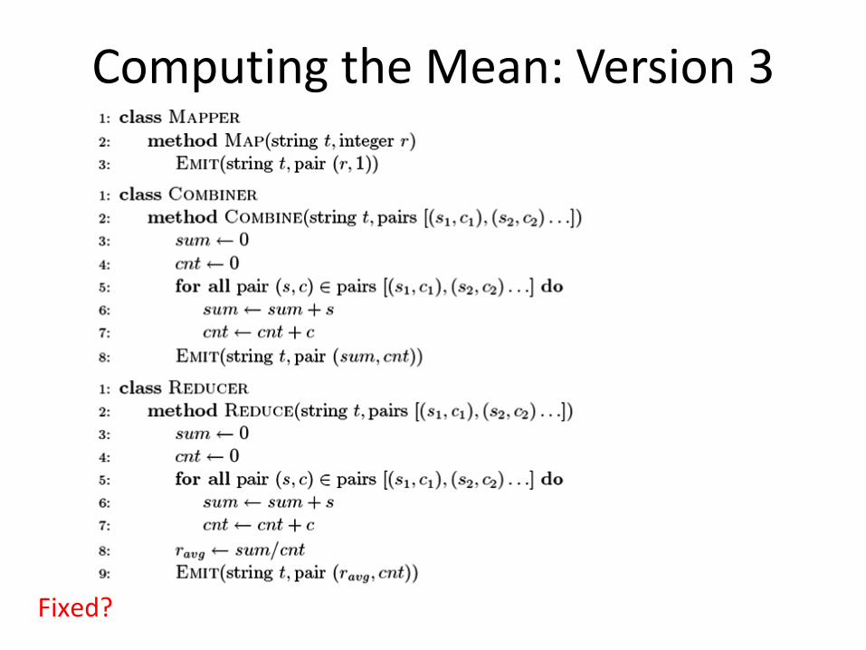
Computing the Mean: Version 3
Fixed?

Computing the Mean: Version 4
Are combiners still needed?

Algorithm Design: Running Example
• Term co-occurrence matrix for a text collection
– M = N x N matrix (N = vocabulary size)
– Mij: number of times i and j co-occur in some context (for concreteness, let’s say context = sentence)
• Why?
– Distributional profiles as a way of measuring semantic distance
– Semantic distance useful for many language processing tasks
MapReduce: Large Counting Problems
• Term co-occurrence matrix for a text collection= specific instance of a large counting problem
– A large event space (number of terms)
– A large number of observations (the collection itself)
– Goal: keep track of interesting statistics about the events
• Basic approach
– Mappers generate partial counts
– Reducers aggregate partial counts
How do we aggregate partial counts efficiently?

First Try: “Pairs”
• Each mapper takes a sentence:
– Generate all co-occurring term pairs
– For all pairs, emit (a, b) → count
• Reducers sum up counts associated with these pairs
• Use combiners!

Pairs: Pseudo-Code

“Pairs” Analysis
• Advantages
– Easy to implement, easy to understand
• Disadvantages
– Lots of pairs to sort and shuffle around (upper bound?)
– Not many opportunities for combiners to work

Another Try: “Stripes”
• Key idea: group together pairs into an associative array
(a, b) → 1
(a, c) → 2
(a, d) → 5
(a, e) → 3
(a, f) → 2
a → { b: 1, c: 2, d: 5, e: 3, f: 2 }
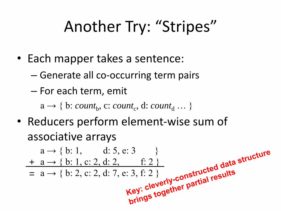
Another Try: “Stripes”
• Each mapper takes a sentence:
– Generate all co-occurring term pairs
– For each term, emit
a → { b: countb, c: countc, d: countd … }
• Reducers perform element-wise sum of associative arrays
a → { b: 1, d: 5, e: 3 }
a → { b: 1, c: 2, d: 2, f: 2 }
a → { b: 2, c: 2, d: 7, e: 3, f: 2 }
+
=

Stripes: Pseudo-Code

“Stripes” Analysis
• Advantages
– Far less sorting and shuffling of key-value pairs
– Can make better use of combiners
• Disadvantages
– More difficult to implement
– Underlying object more heavyweight
– Fundamental limitation in terms of size of event space

Cluster size: 38 cores
Data Source: Associated Press Worldstream (APW) of the English Gigaword Corpus (v3),
which contains 2.27 million documents (1.8 GB compressed, 5.7 GB uncompressed)


Relative Frequencies
• How do we estimate relative frequencies (conditional probabilities) from counts?
– Why do we want to do this?
– How do we do this with MapReduce?
==
'
)',(count
),(count
)(count
),(count)|(
B
BA
BA
A
BAABf

Relative Frequencies: “Stripes”
• Easy!
– One pass to compute (a, *)
– Another pass to directly compute f (B|A)
a → {b1:3, b2 :12, b3 :7, b4 :1, … }

(a, b1) → 3
(a, b2) → 12
(a, b3) → 7
(a, b4) → 1
…
(a, *) → 32
(a, b1) → 3 / 32
(a, b2) → 12 / 32
(a, b3) → 7 / 32
(a, b4) → 1 / 32
…
Reducer holds this value in memory
Relative Frequencies: “Pairs”

Relative Frequencies: “Pairs”
• For this to work:
– Must emit extra (a, *) for every bn in mapper
– Must make sure all a’s get sent to same reducer (use partitioner)
– Must make sure (a, *) comes first (define sort order)
– Must hold state in reducer across different key-value pairs
“Order Inversion”
• Common design pattern
– Computing relative frequencies requires marginal counts
– But marginal cannot be computed until you see all counts
– Buffering is a bad idea!
– Trick: getting the marginal counts to arrive at the reducer before the joint counts
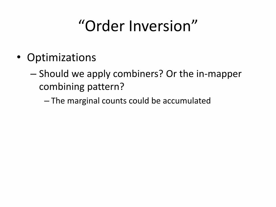
“Order Inversion”
• Optimizations
– Should we apply combiners? Or the in-mapper combining pattern?
– The marginal counts could be accumulated

Synchronization: Pairs vs. Stripes
• Approach 1: Turn synchronization into an ordering problem
– Sort keys into correct order of computation
– Partition key space so that each reducer gets the appropriate set of partial results
– Hold state in reducer across multiple key-value pairs to perform computation
– Illustrated by the “pairs” approach

Synchronization: Pairs vs. Stripes
• Approach 2: Construct data structures that bring partial results together
– Each reducer receives all the data it needs to complete the computation
– Illustrated by the “stripes” approach
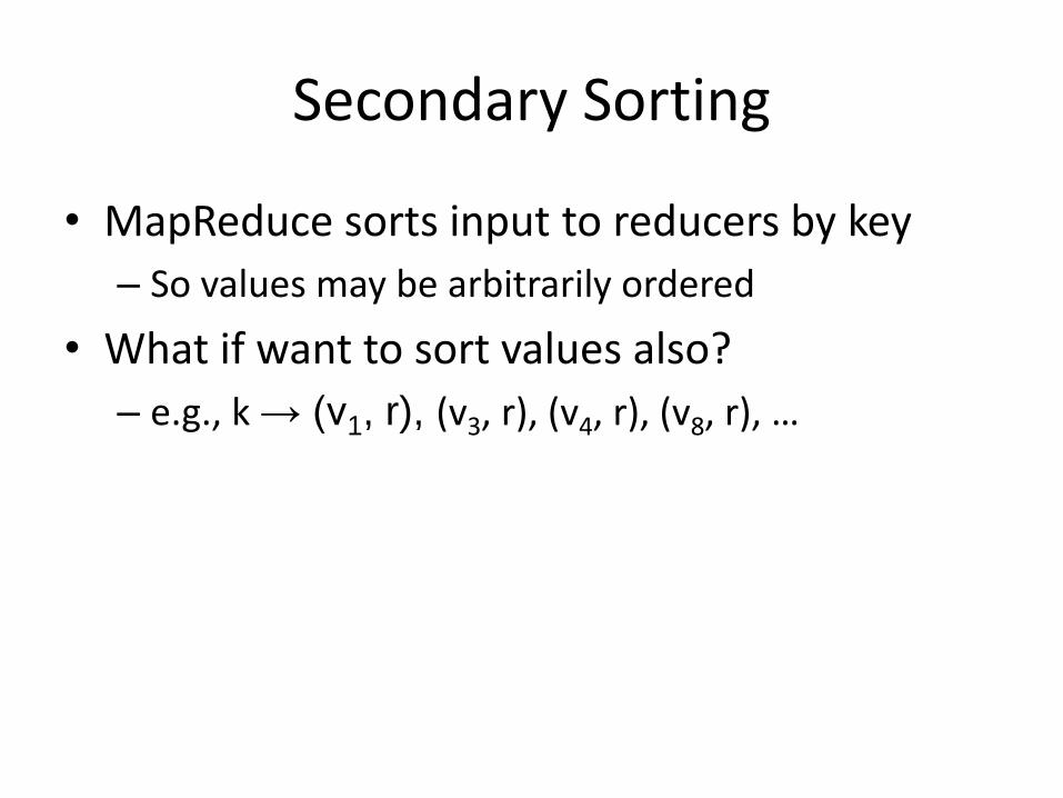
Secondary Sorting
• MapReduce sorts input to reducers by key
– So values may be arbitrarily ordered
• What if want to sort values also?
– e.g., k → (v1, r), (v3, r), (v4, r), (v8, r), …

Secondary Sorting
• Solution 1:
– Buffer values in memory, then sort
– Why is this a bad idea?
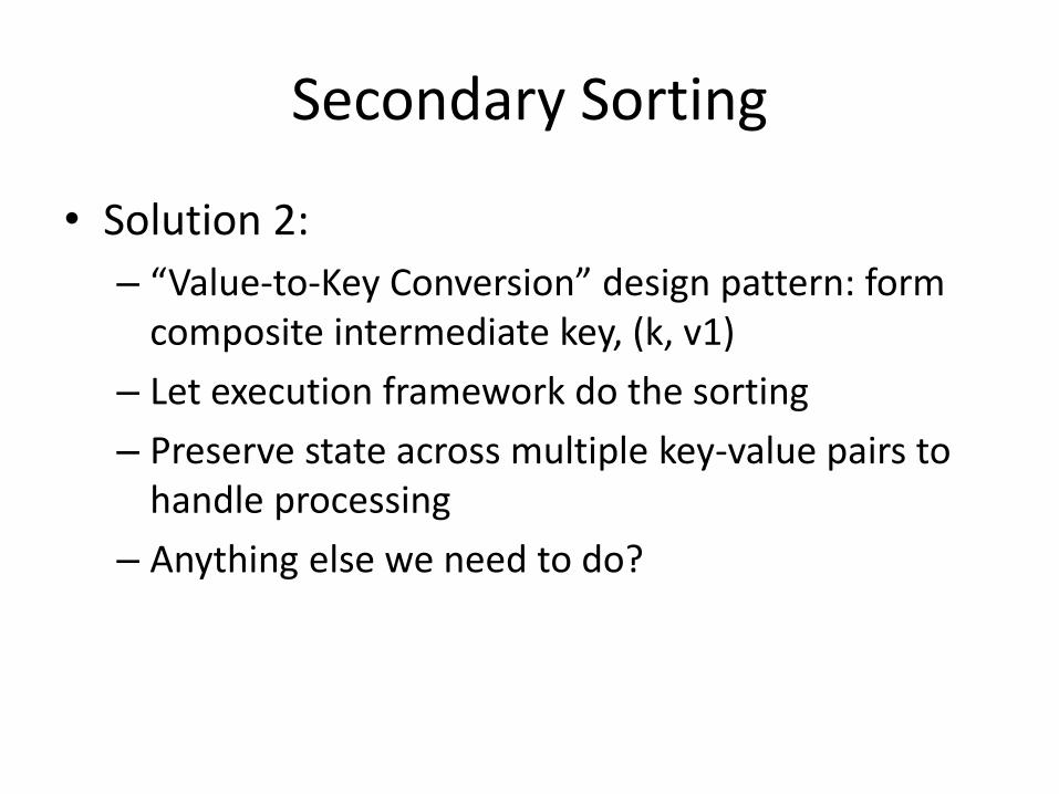
Secondary Sorting
• Solution 2:
– “Value-to-Key Conversion” design pattern: form composite intermediate key, (k, v1)
– Let execution framework do the sorting
– Preserve state across multiple key-value pairs to handle processing
– Anything else we need to do?

“Value-to-Key Conversion”
k → (v1, r), (v4, r), (v8, r), (v3, r)…
(k, v1) → (v1, r)
Before
After
(k, v3) → (v3, r)
(k, v4) → (v4, r)
(k, v8) → (v8, r)
Values arrive in arbitrary order…
…
Values arrive in sorted order…
Process by preserving state across multiple keys
Remember to partition correctly!
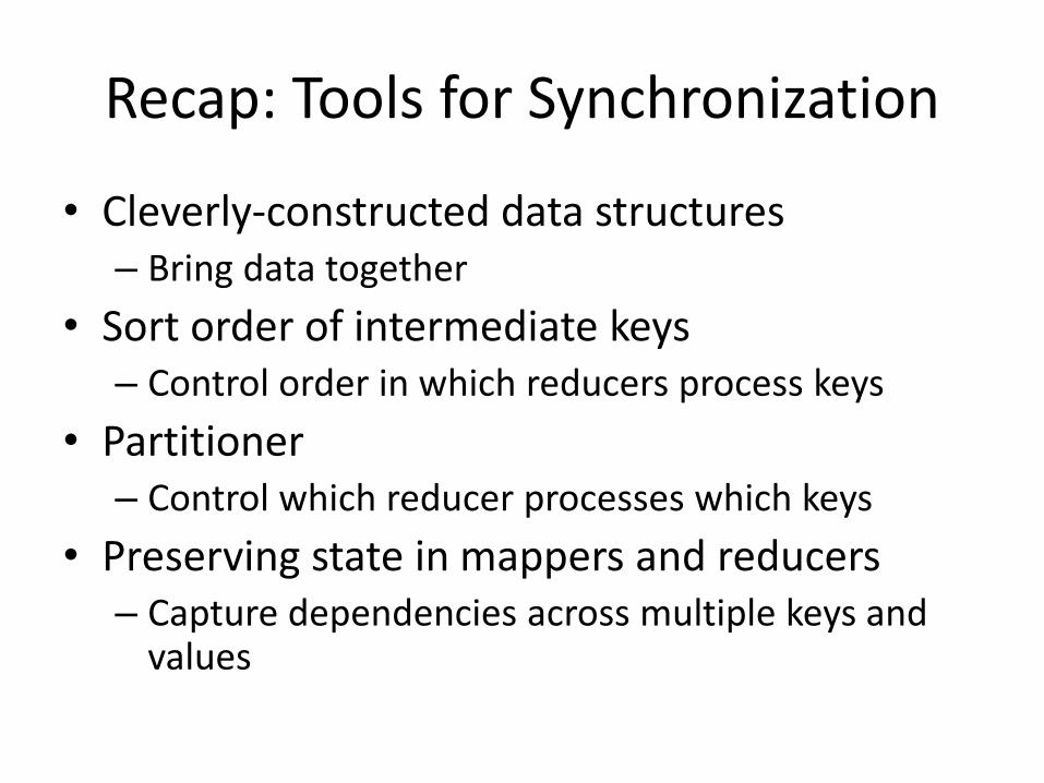
Recap: Tools for Synchronization
• Cleverly-constructed data structures– Bring data together
• Sort order of intermediate keys– Control order in which reducers process keys
• Partitioner– Control which reducer processes which keys
• Preserving state in mappers and reducers– Capture dependencies across multiple keys and
values
Issues and Tradeoffs
• Number of key-value pairs
– Object creation overhead
– Time for sorting and shuffling pairs across the network
• Size of each key-value pair
– De/serialization overhead

Issues and Tradeoffs
• Local aggregation
– Opportunities to perform local aggregation varies
– Combiners make a big difference
– Combiners vs. “In-mapper combining”
– RAM vs. disk vs. network

Take Home Messages
• MapReduce Algorithm Design
– “In-Mapper Combining”
– “Pairs” vs “Stripes”
– “Order Inversion”
– “Value-to-Key Conversion”