developing modeling, optimization, and advanced process
TRANSCRIPT

Brigham Young University Brigham Young University
BYU ScholarsArchive BYU ScholarsArchive
Theses and Dissertations
2016-05-01
Developing Modeling, Optimization, and Advanced Process Developing Modeling, Optimization, and Advanced Process
Control Frameworks for Improving the Performance of Transient Control Frameworks for Improving the Performance of Transient
Energy-Intensive Applications Energy-Intensive Applications
Seyed Mostafa Safdarnejad Brigham Young University
Follow this and additional works at: https://scholarsarchive.byu.edu/etd
Part of the Chemical Engineering Commons
BYU ScholarsArchive Citation BYU ScholarsArchive Citation Safdarnejad, Seyed Mostafa, "Developing Modeling, Optimization, and Advanced Process Control Frameworks for Improving the Performance of Transient Energy-Intensive Applications" (2016). Theses and Dissertations. 6057. https://scholarsarchive.byu.edu/etd/6057
This Dissertation is brought to you for free and open access by BYU ScholarsArchive. It has been accepted for inclusion in Theses and Dissertations by an authorized administrator of BYU ScholarsArchive. For more information, please contact [email protected], [email protected].

Developing Modeling, Optimization, and Advanced Process Control Frameworks for
Improving the Performance of Transient Energy–Intensive Applications
Seyed Mostafa Safdarnejad
A dissertation submitted to the faculty ofBrigham Young University
in partial fulfillment of the requirements for the degree of
Doctor of Philosophy
John D. Hedengren, ChairLarry L. Baxter
Thomas H. FletcherMatthew J. Memmott
Thomas A. Knotts
Department of Chemical Engineering
Brigham Young University
May 2016
Copyright © 2016 Seyed Mostafa Safdarnejad
All Rights Reserved

ABSTRACT
Developing Modeling, Optimization, and Advanced Process Control Frameworks forImproving the Performance of Transient Energy–Intensive Applications
Seyed Mostafa SafdarnejadDepartment of Chemical Engineering, BYU
Doctor of Philosophy
The increasing trend of world-wide energy consumption emphasizes the importance of on-going optimization of new and existing technologies. In this dissertation, two energy–intensivesystems are simulated and optimized. Advanced estimation, optimization, and control techniquessuch as a moving horizon estimator and a model predictive controller are developed to enhance theprofitability, product quality, and reliability of the systems. An enabling development is presentedfor the solution of complex dynamic optimization problems. The strategy involves an initializa-tion approach to large–scale system models that both enhance the computational performance aswell as the ability of the solver to converge to an optimal solution. One particular application ofthis approach is the modeling and optimization of a batch distillation column. For estimation ofunknown parameters, an `1-norm method is utilized that is less sensitive to outliers than a squarederror objective. The results obtained from the simple model match the experimental data and modelprediction for a more rigorous model. A nonlinear statistical analysis and a sensitivity analysis arealso implemented to verify the reliability of the estimated parameters. The reduced–order modeldeveloped for the batch distillation column is computationally fast and reasonably accurate andis applicable for real time control and online optimization purposes. Similar to estimation, an `1-norm objective function is applied for optimization of the column operation. Application of an`1-norm permits explicit prioritization of the multi–objective problems and adds only linear termsto the problem. Dynamic optimization of the column results in a 14% increase in the methanolproduct obtained from the column with 99% purity. In a second application of the methodology,the results obtained from optimization of the hybrid system of a cryogenic carbon capture (CCC)and power generation units are presented. Cryogenic carbon capture is a novel technology for CO2removal from power generation units and has superior features such as low energy consumption,large–scale energy storage, and fast response to fluctuations in electricity demand. Grid–level en-ergy storage of the CCC process enables 100% utilization of renewable power sources while 99%of the CO2 produced from fossil–fueled power plants is captured. In addition, energy demand ofthe CCC process is effectively managed by deploying the energy storage capability of this process.By exploiting time–of–day pricing, the profit obtained from dynamic optimization of this hybridenergy system offsets a significant fraction of the cost of construction of the cryogenic carboncapture plant.
Keywords: dynamic optimization, initialization, batch distillation column, cryogenic carbon cap-ture, power generation, energy storage

ACKNOWLEDGMENTS
I would like to express appreciation for the financial support and technical cooperation from
Sustainable Energy Solutions (SES), without which this work could not have been undertaken. I
am also grateful of the on–demand support, responsiveness, and insightful comments from my PhD
advisor, Prof. John Hedengren. I also appreciate the involvement of Prof. Larry Baxter for invalu-
able direction and advice. I also wish to thank the other members of my committee, Prof. Fletcher,
Prof. Knotts, and Prof. Memmot for their comments and guidance. Jonathan Gallacher, James
Richards, Jeffrey Griffiths, Colin Muir, and many others at Brigham Young University contributed
to this work and I am thankful for their hard work and dedication to the research.
I am also very grateful for the continuous encouragement of my parents and siblings.
Lastly, I wish to recognize my wife, Shima, for her enabling support, encouragement, and company
throughout my graduate school. I would like to dedicate this dissertation to Shima, who deserves
this degree as much as I do.

CONTENTS
List of Tables . . . . . . . . . . . . . . . . . . . . . . . . . . . . . . . . . . . . . . . . . . vii
List of Figures . . . . . . . . . . . . . . . . . . . . . . . . . . . . . . . . . . . . . . . . . viii
NOMENCLATURE . . . . . . . . . . . . . . . . . . . . . . . . . . . . . . . . . . . . . . x
Chapter 1 Introduction . . . . . . . . . . . . . . . . . . . . . . . . . . . . . . . . . . . 11.1 Initialization Strategies and Objective Functions for Estimation and Optimization
of Dynamic Systems . . . . . . . . . . . . . . . . . . . . . . . . . . . . . . . . . 21.2 Batch Distillation Columns . . . . . . . . . . . . . . . . . . . . . . . . . . . . . . 31.3 Hybrid System of Power Generation and Cryogenic Carbon Capture . . . . . . . . 51.4 Outline . . . . . . . . . . . . . . . . . . . . . . . . . . . . . . . . . . . . . . . . 71.5 Main Contributions . . . . . . . . . . . . . . . . . . . . . . . . . . . . . . . . . . 8
Chapter 2 Initialization Strategies for Optimization of Dynamic Systems . . . . . . . 92.1 Introduction . . . . . . . . . . . . . . . . . . . . . . . . . . . . . . . . . . . . . . 9
2.1.1 Simulation and Optimization of DAE Systems . . . . . . . . . . . . . . . 92.1.2 Standard DAE Form . . . . . . . . . . . . . . . . . . . . . . . . . . . . . 112.1.3 DAE Models with Higher Order Derivatives . . . . . . . . . . . . . . . . . 132.1.4 DAE Models with Integral Terms . . . . . . . . . . . . . . . . . . . . . . 132.1.5 DAE Models with Discrete Variables . . . . . . . . . . . . . . . . . . . . 14
2.2 Standard Objective Functions for Estimation and Control . . . . . . . . . . . . . . 142.2.1 Parameter Estimation . . . . . . . . . . . . . . . . . . . . . . . . . . . . . 152.2.2 Control Optimization and Implementation . . . . . . . . . . . . . . . . . . 16
2.3 DAE Initialization Strategies . . . . . . . . . . . . . . . . . . . . . . . . . . . . . 182.3.1 Initialization with Steady-State or Quadratic Approximate Solutions . . . . 192.3.2 Structural Decomposition of DAE Models . . . . . . . . . . . . . . . . . . 202.3.3 Initialization of Higher Index DAE Models . . . . . . . . . . . . . . . . . 22
2.4 Case Studies on Dynamic Initialization . . . . . . . . . . . . . . . . . . . . . . . . 232.4.1 Pendulum Motion: Higher Index DAE Forms . . . . . . . . . . . . . . . . 232.4.2 Linear Initialization: CSTR Case Study . . . . . . . . . . . . . . . . . . . 282.4.3 Tethered Aerial Pipeline Inspection: Initialization with Sequential Simu-
lation . . . . . . . . . . . . . . . . . . . . . . . . . . . . . . . . . . . . . 312.4.4 Smart Grid Energy System: Structural Decomposition . . . . . . . . . . . 34
2.5 Conclusions . . . . . . . . . . . . . . . . . . . . . . . . . . . . . . . . . . . . . . 38
Chapter 3 Framework for Dynamic Parameter Estimation and Optimization . . . . 393.1 Introduction . . . . . . . . . . . . . . . . . . . . . . . . . . . . . . . . . . . . . . 39
3.1.1 Confidence Intervals and Sensitivity Analysis . . . . . . . . . . . . . . . . 423.2 Dynamic Estimation and Optimization for a Batch Distillation Column . . . . . . 44
3.2.1 Apparatus and Experimental Procedure . . . . . . . . . . . . . . . . . . . 443.2.2 Equations for the Simplified Process Model . . . . . . . . . . . . . . . . . 46
iv

3.2.3 Equations for the Detailed Process Model . . . . . . . . . . . . . . . . . . 483.2.4 Model Validation . . . . . . . . . . . . . . . . . . . . . . . . . . . . . . . 513.2.5 Testing the Reliability of the Estimated Parameters . . . . . . . . . . . . . 533.2.6 Model Optimization and Validation . . . . . . . . . . . . . . . . . . . . . 56
3.3 Conclusions . . . . . . . . . . . . . . . . . . . . . . . . . . . . . . . . . . . . . . 58
Chapter 4 Hybrid System of Cryogenic Carbon Capture and Power Generation Units 604.1 Introduction . . . . . . . . . . . . . . . . . . . . . . . . . . . . . . . . . . . . . . 604.2 Non-energy-storing Version of the Cryogenic Carbon Capture (CCC) . . . . . . . . 654.3 Modeling Framework for the Non-energy-storing Hybrid System . . . . . . . . . . 66
4.3.1 Model Equations . . . . . . . . . . . . . . . . . . . . . . . . . . . . . . . 664.3.2 Controlled variable . . . . . . . . . . . . . . . . . . . . . . . . . . . . . . 754.3.3 Constraints . . . . . . . . . . . . . . . . . . . . . . . . . . . . . . . . . . 76
4.4 Model Implementation . . . . . . . . . . . . . . . . . . . . . . . . . . . . . . . . 774.4.1 Model Inputs . . . . . . . . . . . . . . . . . . . . . . . . . . . . . . . . . 77
4.5 Optimization Results . . . . . . . . . . . . . . . . . . . . . . . . . . . . . . . . . 784.5.1 Comparison Between Summer and Winter Results . . . . . . . . . . . . . 784.5.2 Sensitivity Analysis for Wind Power Adoption . . . . . . . . . . . . . . . 83
4.6 Conclusion . . . . . . . . . . . . . . . . . . . . . . . . . . . . . . . . . . . . . . 85
Chapter 5 Investigating the Impact of Energy-Storing Cryogenic Carbon Captureon Power Plant Performance . . . . . . . . . . . . . . . . . . . . . . . . . 87
5.1 Introduction . . . . . . . . . . . . . . . . . . . . . . . . . . . . . . . . . . . . . . 875.2 Example Case Study for Energy Storage Concept . . . . . . . . . . . . . . . . . . 905.3 Modeling Framework for the Energy-Storing Hybrid System . . . . . . . . . . . . 92
5.3.1 Governing Equations . . . . . . . . . . . . . . . . . . . . . . . . . . . . . 925.3.2 Constraints . . . . . . . . . . . . . . . . . . . . . . . . . . . . . . . . . . 94
5.4 Model Inputs . . . . . . . . . . . . . . . . . . . . . . . . . . . . . . . . . . . . . 955.5 Results and Discussion . . . . . . . . . . . . . . . . . . . . . . . . . . . . . . . . 98
5.5.1 Sensitivity Analysis . . . . . . . . . . . . . . . . . . . . . . . . . . . . . 1065.6 Conclusion . . . . . . . . . . . . . . . . . . . . . . . . . . . . . . . . . . . . . . 108
Chapter 6 Dynamic Optimization of a Hybrid System of Cryogenic Carbon Captureand a Baseline Power Generation Unit . . . . . . . . . . . . . . . . . . . . 109
6.1 Introduction . . . . . . . . . . . . . . . . . . . . . . . . . . . . . . . . . . . . . . 1096.2 Model Adjustment for Baseline Performance . . . . . . . . . . . . . . . . . . . . 1096.3 Results and Discussion . . . . . . . . . . . . . . . . . . . . . . . . . . . . . . . . 1106.4 Comparison Between Combined and Simple Cycles . . . . . . . . . . . . . . . . . 1156.5 Comparison of Cycling Costs . . . . . . . . . . . . . . . . . . . . . . . . . . . . . 1186.6 Conclusion . . . . . . . . . . . . . . . . . . . . . . . . . . . . . . . . . . . . . . 121
Chapter 7 Conclusion and Future Work . . . . . . . . . . . . . . . . . . . . . . . . . 1237.1 Conclusion . . . . . . . . . . . . . . . . . . . . . . . . . . . . . . . . . . . . . . 1237.2 Future Work . . . . . . . . . . . . . . . . . . . . . . . . . . . . . . . . . . . . . . 126
7.2.1 Batch Distillation Column . . . . . . . . . . . . . . . . . . . . . . . . . . 127
v

7.2.2 Hybrid System of Power Generation and the CCC Process . . . . . . . . . 1277.3 Publications . . . . . . . . . . . . . . . . . . . . . . . . . . . . . . . . . . . . . . 129
Bibliography . . . . . . . . . . . . . . . . . . . . . . . . . . . . . . . . . . . . . . . . . . 131
Appendix A Rigorous Model for the Batch Distillation Column . . . . . . . . . . . . . 145
vi
LIST OF TABLES
2.1 Nomenclature for general form of the objective function with `1-norm formulationfor dynamic data reconciliation . . . . . . . . . . . . . . . . . . . . . . . . . . . . 16
2.2 Nomenclature for general form of the objective function with `1-norm formulationfor dynamic optimization . . . . . . . . . . . . . . . . . . . . . . . . . . . . . . . 17
2.3 Summary of Case Studies . . . . . . . . . . . . . . . . . . . . . . . . . . . . . . . 242.4 Summary of Initialization Results with APOPT . . . . . . . . . . . . . . . . . . . 272.5 Summary of DAE Initialization Results with IPOPT . . . . . . . . . . . . . . . . . 272.6 CSTR MPC comparison of linear pre-solve, block diagonal decomposition, and no
initialization . . . . . . . . . . . . . . . . . . . . . . . . . . . . . . . . . . . . . . 312.7 Tethered UAV comparison of linear pre-solve, block diagonal decomposition, and
no initialization . . . . . . . . . . . . . . . . . . . . . . . . . . . . . . . . . . . . 342.8 Computation time for hybrid system of a CCC process and power generation units . 37
3.1 Confidence interval calculation for the four parameter case . . . . . . . . . . . . . 51
4.1 Summary of the input parameters . . . . . . . . . . . . . . . . . . . . . . . . . . . 704.2 Coal properties . . . . . . . . . . . . . . . . . . . . . . . . . . . . . . . . . . . . 714.3 Natural gas properties . . . . . . . . . . . . . . . . . . . . . . . . . . . . . . . . . 72
5.1 Additional input parameters for the case with energy storage . . . . . . . . . . . . 98
6.1 Summary of cycling costs . . . . . . . . . . . . . . . . . . . . . . . . . . . . . . . 121
vii

LIST OF FIGURES
1.1 Overview of methodology for batch column optimization with novel contributionsunderlined . . . . . . . . . . . . . . . . . . . . . . . . . . . . . . . . . . . . . . . 4
2.1 DAE model equations are discretized and solved over a time horizon. . . . . . . . 122.2 Flowchart for initialization of DAE systems . . . . . . . . . . . . . . . . . . . . . 192.3 Two initialization cases for demonstration of infeasibility detection and a final op-
timal case . . . . . . . . . . . . . . . . . . . . . . . . . . . . . . . . . . . . . . . 212.4 Problem is decomposed into independent variables and equations . . . . . . . . . . 222.5 Pendulum motion . . . . . . . . . . . . . . . . . . . . . . . . . . . . . . . . . . . 242.6 Solution to Index-0 to Index-3 DAE model forms . . . . . . . . . . . . . . . . . . 252.7 Lower block triangular form for pendulum data reconciliation . . . . . . . . . . . 262.8 Continuously Stirred Tank Reactor . . . . . . . . . . . . . . . . . . . . . . . . . . 282.9 Uncontrolled linear and nonlinear response . . . . . . . . . . . . . . . . . . . . . 292.10 Nonlinear MPC solution with linear MPC initialization . . . . . . . . . . . . . . . 302.11 Lower block triangular form for nonlinear MPC of a CSTR . . . . . . . . . . . . . 302.12 Lower block triangular form for a tethered UAV . . . . . . . . . . . . . . . . . . . 322.13 A simulated tethered UAV performs surveillance of a pipeline. . . . . . . . . . . . 332.14 Hybrid system of CCC process and power generation units . . . . . . . . . . . . . 352.15 Lower block triangular form for hybrid system of CCC process and power genera-
tion units . . . . . . . . . . . . . . . . . . . . . . . . . . . . . . . . . . . . . . . 352.16 Power and demand profiles for the hybrid system of CCC process and power gen-
eration units . . . . . . . . . . . . . . . . . . . . . . . . . . . . . . . . . . . . . . 37
3.1 Overview of methodology for batch column optimization with novel contributionsunderlined . . . . . . . . . . . . . . . . . . . . . . . . . . . . . . . . . . . . . . . 41
3.2 Apparatus used for the experiments . . . . . . . . . . . . . . . . . . . . . . . . . 453.3 Non-optimized base case where the final required purity (> 99 mol% ethanol) is
not met . . . . . . . . . . . . . . . . . . . . . . . . . . . . . . . . . . . . . . . . 463.4 Model validation for initial parameter estimation . . . . . . . . . . . . . . . . . . 523.5 Insensitivity of the `1-norm estimation to outliers compared to the squared error
objective . . . . . . . . . . . . . . . . . . . . . . . . . . . . . . . . . . . . . . . . 523.6 Scaled variable sensitivities to the parameters . . . . . . . . . . . . . . . . . . . . 543.7 Magnitude of singular values from singular value decomposition reveals indepen-
dent linear combinations of parameters to reconcile data . . . . . . . . . . . . . . 553.8 Contour and surface plots of the objective function value for values of heater ef-
ficiency(h f)
and vapor efficiency (EMV ). The 95% confidence interval for the`1-norm is not correct (future work) and the confidence interval for the squarederror is an approximation. . . . . . . . . . . . . . . . . . . . . . . . . . . . . . . . 56
3.9 Model validation for final parameter estimates . . . . . . . . . . . . . . . . . . . . 573.10 Reflux ratio for optimized control scheme compared to the non-optimized base case 573.11 Optimized control scheme compared to the non-optimized base case and to the
model prediction . . . . . . . . . . . . . . . . . . . . . . . . . . . . . . . . . . . 58
viii

4.1 Schematic configuration of the integrated system of power generation unit and theCCC process without energy storage . . . . . . . . . . . . . . . . . . . . . . . . . 67
4.2 2022 forecasted electricity demand data for a zone in southern California, USA(Summer case) [172]. . . . . . . . . . . . . . . . . . . . . . . . . . . . . . . . . . 78
4.3 2022 forecasted electricity demand data for a zone in southern California, USA(Winter case) [172]. . . . . . . . . . . . . . . . . . . . . . . . . . . . . . . . . . . 79
4.4 Power vs. electricity demand profile (summer case) . . . . . . . . . . . . . . . . . 804.5 Power vs. electricity demand profile (winter case) . . . . . . . . . . . . . . . . . . 814.6 Natural gas imported to the plant . . . . . . . . . . . . . . . . . . . . . . . . . . . 824.7 LNG production in the system . . . . . . . . . . . . . . . . . . . . . . . . . . . . 844.8 Impact of wind power adoption factor on power production from gas and coal
(winter data) . . . . . . . . . . . . . . . . . . . . . . . . . . . . . . . . . . . . . . 854.9 Operating costs and electricity demand revenue vs wind power adoption factor (α)
(winter data) . . . . . . . . . . . . . . . . . . . . . . . . . . . . . . . . . . . . . . 86
5.1 Schematic configuration of the integrated system of power generation unit and theCCC process with energy storage . . . . . . . . . . . . . . . . . . . . . . . . . . . 89
5.2 Results for the simplified case of energy storage . . . . . . . . . . . . . . . . . . . 925.3 Actual electricity demand for San Diego, USA, and average power price for Cali-
fornia for the period between September 13, 2014 and September 20, 2014 [177,178]. 965.4 Actual wind power data for the period between September 13, 2014 and September
20, 2014 [177]. . . . . . . . . . . . . . . . . . . . . . . . . . . . . . . . . . . . . 975.5 Electricity demand vs. power production . . . . . . . . . . . . . . . . . . . . . . . 1005.6 Increased value of wind power by using energy storage of the CCC . . . . . . . . . 1025.7 LNG inventory, LNG production, and LNG required to run the CCC vs. power price1035.8 Natural gas imported and exported vs. power price . . . . . . . . . . . . . . . . . 1045.9 Demand curves for natural gas compressor, mixed refrigerant compressor, and
CCC plant . . . . . . . . . . . . . . . . . . . . . . . . . . . . . . . . . . . . . . . 1065.10 Comparison between power demand of mixed refrigerant compressor with and
without energy storage . . . . . . . . . . . . . . . . . . . . . . . . . . . . . . . . 107
6.1 Total power generation from the steam turbine vs. wind power . . . . . . . . . . . 1116.2 Electricity demand and power production from coal, wind, and natural gas . . . . . 1126.3 Trend of natural gas and LNG inventory . . . . . . . . . . . . . . . . . . . . . . . 1146.4 Electricity demand for refrigeration compressors and CCC plant in a combined
cycle power generation unit with energy storage . . . . . . . . . . . . . . . . . . . 1156.5 Excess power comparison between combined and simple power generation cycles
with and without energy storage, respectively . . . . . . . . . . . . . . . . . . . . 1176.6 Electricity demand for refrigeration compressors and CCC plant in a simple cycle
power generation unit without energy storage . . . . . . . . . . . . . . . . . . . . 118
7.1 Power supply curve for Southeastern Electric Reliability Council region [195] . . . 129
ix

NOMENCLATURE
C Mass flow rate of the coal combustionCCC Cryogenic carbon captureCCCECL Cryogenic carbon capture with an external cooling loopCCS Carbon capture and storageCHP Combined heat and power unitD Distillate mole flow rateDCCC Total electricity demand for the CCC facilityDLNG Total electricity demand of the LNG production facilityDMR Work of compression of the mixed refrigerant compressorDNG Work of compression of the natural gas compressorDNG Work of compression of the pipeline compressorDplant Combined electricity demand of the CCC and LNG production facilitiesDplant,max Maximum fraction of the combined electricity demand of the LNG and CCC plantsDRes Electricity demand of the residential usersDTot Total electricity demandEMV Murphree efficiencyEGS Enhanced geothermal systemEPA Environmental Protection Agencyfcond Fraction of the initial reboiler charge in the condenserftray Fraction of the initial reboiler charge on each trayFGC Mass flow rate of the flue gas produced from coal combustionFGNG Mass flow rate of the flue gas produced from natural gas combustionFGNG,max Maximum mass flow rate of the flue gas produced from natural gas combustionFOMCT Fixed operating and maintenance costs of the coal–fired power generation unitFOMGT Fixed operating and maintenance costs of the gas–fired power generation unitGPCC
max Maximum permitted power production in the combined cycleGT cap Capacity of the gas turbinehdot Heat input from the reboilerh f Heating efficiencyhL Liquid EnthalpyhV Vapor EnthalpyHvap Heat of vaporization for the mixtureHHV Higher heating valueIEA International Energy AgencyIGCC Integrated Gasification Combined CycleKNG Gain for the natural gas intakeKST Gain for power production in the steam boilerL Liquid mole flow rateLCOE Levelized Cost of ElectricityLNG Liquefied natural gasLNGBY P Mass flow rate of the LNG bypassing the tankLNGFrom Tank Mass flow rate of the LNG from the tankLNGProd Mass flow rate of the LNG production
x

LNGTank Mass of the LNG in the tankLNGTo Tank Mass flow rate of the LNG directed to the tankLNGR Total mass flow rate of the LNG demandMR Mass flow rate of the mixed refrigerantn Number of traysNcond Number of moles in the condensernp Number of product molesNreb Number of moles in the reboilerNreb,init Initial number of moles in the reboilerNtray Number of liquid moles on each trayNG Natural gasNGCCC Mass flow rate of the natural gas coming from the natural gas compressorNGConv Mass flow rate of the natural gas combustion in the gas turbineNGConv,max Maximum mass flow rate of the combusted natural gasNGEXPT Mass flow rate of the natural gas exported to the pipelineNGOnephase Mass flow rate of the natural gas coming from the LNG/mixed refrigerant recuperatorNGPL Mass flow rate of the natural gas imported from the pipelineNGPL,SP Set point of the natural gas imported from the pipelineNGTot Total mass flow rate of the natural gas for liquefactionNGTwophase Mass flow rate of the two phase natural gas coming from the CCC plantNGCC Natural gas combined cycleOCR Organic Rankine cycleP PressurePC Coal pricePCT Power generated from the coal–generated flue gasPE Energy pricePEx Excess power productionPGT Power production in the gas turbinePN Natural gas pricePNGCC Power generated from the natural gas flue gasPSP Set point of the power output in the steam boilerPSP,Max Upper bound for the set point of the power output from the coal-fired steam boilerPST Total power production in the steam boilerPTot Total power generationPW Power generated from the windPsat
i Saturated pressure of tray iPC Pulverized CoalQg Total heat gain in the recuperatorQl Total heat loss in the recuperatorQcond Condenser cooling loadQreb Reboiler heating rateR Reflux ratioSAPG Solar Aided Power Generationt Time
xi

Ti Temperature of tray iV Vapor mole flow rateVOMCT Variable operating and maintenance costs of the coal–fired power generation unitVOMGT Variable operating and maintenance costs of the gas–fired power generation unitxcond Composition in the condenserxp Product compositionxreb Composition in the reboilerxn Liquid mole fractionyn Actual mole fractiony∗n Equilibrium vapor mole fractionδP Pressure drop∆H1 Enthalpy difference of the cold natural gas across the recuperator∆H2 Enthalpy difference of the cold mixed refrigerant across the recuperator∆H3 Enthalpy difference of the warm natural gas across the recuperator∆H4 Enthalpy difference of the warm mixed refrigerant across the recuperator∆HC
FG Specific enthalpy change of the flue gas from combustion of coal∆Hg Enthalpy of combustion of natural gas∆HNG
FG Specific enthalpy change of the flue gas from combustion of natural gasεg Efficiency of power production in the gas turbineεSB Efficiency of the heat exchange in steam reboilerηST Efficiency of the steam turbineγi Activity coefficientτNG Time constant for the natural gas intakeτST Time constant for power production in the steam boiler
xii

CHAPTER 1. INTRODUCTION
The economic and environmental desires to reduce industrial energy consumption drives
ongoing optimization of the new and existing technologies important in engineering. For exam-
ple, large-scale continuous distillation columns have been the focus of optimization since the first
column was built. However, the transient nature of batch columns has caused many to remain
unoptimized which results in more energy consumption than is likely needed and an opportunity
for improvement. This emphasizes the continuous need for optimization of the existing units in-
cluding continuous and batch distillation columns. Another important area that would benefit from
optimization is energy generation. While new technologies for power production, such as fuel
cells, and new energy sources such as renewable energy, show promise, they cannot yet replace a
grid–scale thermal power unit. Therefore, fossil–fueled power plants will continue to play a ma-
jor role in power sector. Optimizing the operation of fossil–fueled power plants typically means
increasing the efficiency of the system which also results in lower CO2 emission. Although ef-
ficiency improvement reduces the CO2 emission from these power plants, it is not adequate to
achieve the target CO2 emission level of the Clean Power Plan enforced by the environmental pro-
tection agency (EPA). Thus, optimization of the existing units should accompany the technology
development in finding ways to reduce CO2 emission from fossil power plants.
Developing modeling frameworks for estimation, optimization, and control of these two
key industrial applications (batch distillation and power plant carbon reduction) is a focus of this
dissertation. These two application areas are complex and require large–scale differential and al-
gebraic equation models to describe their dynamic behavior. A fundamental contribution of this
work is to not only optimize these two particular applications, but also to develop methods to
initialize and efficiently solve large–scale and complex system models. Developing initialization
strategies for large–scale nonlinear systems is described in Chapter 2. In Chapter 3, a mathematical
modeling framework is developed for a batch distillation column. In this case, the purpose is to de-
1

velop a simple model that takes advantage of a moving horizon estimator for parameter estimation
and a model predictive controller for maximization of the column product while staying within
the product quality limits. Chapters 4-6 develop a mathematical model for the integrated system
of a cryogenic carbon capture and power generation units. This work includes power production
from fossil-fueled and renewable power plants with consideration of the energy–storing version
of cryogenic carbon capture. The goal of this application is to maximize the profitability of the
hybrid system such that it can meet the overall electricity demand and capture 90% of the CO2
emissions from the fossil-fueled power plants. A model predictive control framework is utilized in
this application to optimize the operation of the hybrid system.
While this study considers two specific applications in the energy industry, they are pre-
sented in a modular basis. The estimation and control frameworks developed in this dissertation
are applicable to similar systems of batch distillation or energy production, but are also applicable
more generally to optimize complex dynamic systems.
1.1 Initialization Strategies and Objective Functions for Estimation and Optimization ofDynamic Systems
The large-scale dynamic applications considered in this study are non-convex and non-
linear, i.e. there are local optimal points and the solution cannot be found from a single matrix
inversion. Consequently, the solver may not be able to find a successful solution. In addition,
many variables and equations define these systems and their time–dependence. Thus, a good
initialization strategy is necessary to find a successful solution with a reasonable computational
time. Several techniques have been utilized to initialize these nonlinear systems. These techniques
include initialization from a steady–state or a linear solution of the problem, structural decomposi-
tion of the differential and algebraic equations (DAEs), and initialization from the sequential and
simultaneous simulation of the problem. Developing initialization strategies for these nonlinear
systems is the foundation of further analysis of the two industrial applications considered in this
dissertation. Chapter 2 details these initialization strategies.
In two applications, new techniques for estimation, optimization, and control are used to
develop the modeling frameworks. These techniques include moving horizon estimation (MHE)
and model predictive control (MPC) that benefit from an objective function in the form of an `1-
2

-norm. An `1- norm objective function has superior performance to the conventional least square
techniques. The details of an `1- norm objective function for estimation and optimization purposes
are discussed in details in Chapter 2.
1.2 Batch Distillation Columns
Many specialty and smaller-use items are often processed in batch distillation columns. The
transient nature of batch columns has caused many to remain unoptimized. Work on batch columns
has increased in the last 30 years as computers have become more sophisticated, and several stud-
ies have considered both advanced solving techniques and advanced column configurations. The
models developed for batch column optimization generally fall into two categories: first-principles
models and shortcut or simple models. First-principles models are those with governing mass
and energy balance equations, detailed thermodynamics, tray dynamics, system non-idealities and
variable flow rates. While these models are more accurate, the use of these models has been lim-
ited due to high computational costs. The second class of models, shortcut models, has received
far greater attention. These models contain less physics and are generally used for estimates and
comparative studies. The primary purpose of these models is to create an accurate, computation-
ally fast simulation for use in design and control of batch columns. While these models achieve
the reduction in computational load, the lack of experimental data makes it difficult to determine
the accuracy of these models. The assumptions made in these models also limit their use to ideal
systems.
The gap between first-principles models and shortcut models is large. First-principles mod-
els can provide predictions for many systems but require thermodynamic and physical property
models as inputs, while the assumptions in shortcut models make them applicable only to a small
class of relatively ideal systems. In this dissertation, a method is proposed for developing shortcut
models with relaxed assumptions. The method is based on fitting parameters in place of simpli-
fying assumptions to include system non-idealities without solving the first-principles equations.
Empirical model regression requires extensive experimental data whereas first-principles models
typically need less data to determine unknown parameters, being based on fundamental correla-
tions. Dynamic parameter estimation can be used to reduce the experimental load. The case study
presented in this dissertation required only one experiment to determine model parameters. As
3

Figure 1.1: Overview of methodology for batch column optimization with novel contributions underlined
with any model containing fitting parameters, there is concern over the accuracy of the parameters.
By using nonlinear statistics and a model sensitivity analysis, it is possible to determine how many
parameters can be estimated from the collected data and the acceptable range for those parameters.
These steps are shown in Figure 1.1 and form the heart of the method. Underlined elements of the
methodology indicate the new approach to batch separation systems.
The well-known methodology shown in Figure 1.1 is applied to an experimental case study.
The methodology includes the use of `1-norm dynamic parameter estimation, nonlinear statistics,
and a model parameter sensitivity analysis. These techniques are applied together to a batch dis-
tillation column in a holistic approach to dynamic optimization. Models developed using this
method account for system non-idealities not seen in typical shortcut models without sacrificing
computational speed. The fast solution time of the models developed in this study allows for their
4

utilization in real–time control and online optimization applications. The novel contributions of
this study are:
• Development of a reduced–order model that is suitable for real–time control
• Application of an `1-norm objective function for estimation and optimization
• Nonlinear statistical analysis with approximate multivariate confidence regions
• Model validation for both estimation and optimization
1.3 Hybrid System of Power Generation and Cryogenic Carbon Capture
The second application considers a hybrid system of power generation units and cryogenic
carbon captureTM (CCC). The key to achieve target levels of CO2 emissions in the power sec-
tor is to integrate fossil-fueled power generation plants with a carbon capture system. Although
various methods have been developed for CO2 capture, a major drawback of most CO2 removal
systems is the parasitic energy load. Cryogenic carbon captureTM is a novel technology for CO2
separation from power plant flue gas and is less energy intensive compared to the conventional
capture systems. The CCC process cools flue gas from power generation units to the point that
CO2 desublimates. The process then separates solid CO2 from the remaining gas and melts it.
Both the remaining flue gas and pressurized solid CO2 warm back to higher temperatures.
The CCC process captures CO2 in the flue gas through desublimation. The CCC process
requires two refrigeration loops that consume most of the energy. The CCC process, however, has
some configurations that store energy in the form of a refrigerant. In the energy–storing version,
CCC generates refrigerant during non–peak hours and stores it in insulated vessels for peak hour
usage, thereby replacing the compressor energy with the stored refrigerant. This causes the refrig-
erant production rate to decrease during peak hours, which decreases the energy demand required
by the CCC process for as long as the stored refrigerant is available. With the decreased demand,
more power is available during peak hours relative to the baseline coal boiler rated capacity. In this
dissertation, storage of only one of the refrigerants is considered as it provides more energy during
the recovery mode. Although other refrigerants could be selected, the refrigerant considered for
this purpose is LNG. In addition, during the energy recovery mode of the CCC, a gas turbine can
5

provide more power through the combustion of a fraction of the LNG after it goes through the
CCC process and is converted to natural gas.
Additionally, the LNG generation and storage cycle primarily involves compressors and
heat exchangers; therefore, the storage/recovery or load changing response time is fast (seconds)
compared to that of the steam boilers (hours). The faster energy storage response time is well
matched to intermittent sources like wind turbines and enables the conventional power generation
systems to follow rapidly changing loads. This results in an easier integration of thermal power
generation systems with renewable intermittent power supplies. As renewable energy sources
become a larger portion of the energy market, the significance of rapidly responding to large fluc-
tuations with energy storage becomes critical to maintaining a reliable and cost–effective electric
grid. Storage capacity of LNG vessels also allows scaling from the proposed energy storage to
large–scale systems.
Sustainable Energy Solutions developed the CCC process and energy–storing capabilities
and the detailed models that determine system energy demand and response time. The novel
contributions of this study include developing grid–level models and optimizing CCC in the context
of grid performance. Some of the novel contributions of this work are:
• Dynamic integration of the CCC process with baseline and load–following power generation
units
• Application of the grid–level energy storage facilities for load management
• Full utilization of wind power and optimizing the contribution to the grid
• Enhanced operational flexibility of the integrated energy system
• Reduction in cycling costs of power generation units by using energy storage
• Quantification of impact of energy storage in meeting the demand in combined and simple
cycles power generation units
6

1.4 Outline
This dissertation is divided into 5 chapters. Chapter 2 describes the initialization strategies
developed to achieve a successful solution and to decrease the simulation time for estimation and
control of dynamic applications. These initialization strategies are first demonstrated on simple
problems and they build the foundation for more complex systems such as the applications used in
this dissertation. In addition, the standard frameworks for modeling, estimation, and control of the
applications used in this dissertation are discussed in Chapter 2. These frameworks benefit from an
`1-norm objective function in which has a superior performance over the conventional least square
techniques.
Chapter 3 describes a systematic approach to develop a simple model for optimization of a
batch distillation column. The details of the simple model developed for a batch distillation column
and the experimental procedures taken to verify the model are discussed in this chapter. The results
from the simple model are also compared to a more rigorous model. A nonlinear statistics analysis,
a parameter ranking, and a sensitivity analysis are also described in verifying the accuracy of the
model. The last section of this chapter describes the optimization of the column with the simplified
model and the validation of the optimization results.
Chapter 4 investigates the dynamic integration of cryogenic carbon capture with power
generation units. This chapter includes a mathematical model developed for the non-energy-storing
version of the hybrid system. First, application of the model in summer and winter conditions is
discussed. Then, the impact of increasing the contribution of wind power in meeting the electricity
demand on profitability of a hybrid system without energy storage is reported. A key result is that
there is a maximum wind energy adoption fraction beyond which the intermittent power source is
not fully utilized.
Chapter 5 considers the performance of a hybrid system of power generation units and an
energy storing version of cryogenic carbon capture. The model developed in Chapter 4 is modified
in this chapter to account for energy storage and export of natural gas to a pipeline. The coal–
fired power generation unit considered in this chapter is able to load follow without excess energy
production.
Chapter 6 considers the performance of a hybrid system of a CCC process and power
generation unit in which the coal–fired plant operates as a baseline unit. In addition, the impact of
7

energy storage on reduction of the cycling cost of a power plant in following the electricity load is
presented in this chapter. This chapter continues with a comparison between a typical power plant
that has a CO2 capture process, a simple cycle peaking unit, and a combined cycle unit.
Chapter 7 presents the main highlights of this dissertation followed by a discussion for
future research directions.
1.5 Main Contributions
The main contributions of this dissertation are summarized as following:
• Initialization strategies for optimization of dynamic systems, Chapter 2.
• Reduced–order models and validation of dynamic parameter estimation and optimization for
batch distillation, Chapter 3.
• Modeling hybrid systems of cryogenic carbon capture and baseline power generators and
investigating the impact of cryogenic carbon capture on the performance of power plants,
Chapter 4.
• Grid–level dynamic optimization of cryogenic carbon capture with energy storage, load–
following conventional, and renewable power sources, Chapter 5.
• Hybrid system of cryogenic carbon capture and baseline power generators including both
peaking and combined cycle units, Chapter 6.
8

CHAPTER 2. INITIALIZATION STRATEGIES FOR OPTIMIZATION OF DYNAMICSYSTEMS
2.1 Introduction
Differential and algebraic equations (DAEs) are natural expressions of many physical sys-
tems found in business, mathematics, systems biology, engineering, and science. In business, the
supply chain can be optimized by modeling the storage, production, and consumption through-
out a network [1]. In mathematics, ordinary (ODEs) or partial differential equations (PDEs) are
used to describe certain classes of boundary value problems. In engineering, these equations result
from material, energy, momentum, and force balances [2]. In science, laws of motion are naturally
described by differential equations that relate position, velocity, and acceleration [3, 4].
Just as differential equations naturally describe many systems, these same equations can
also be used to optimize among many potential designs or feasible solutions. One difference
between static or steady-state models and dynamic models is that optimal solutions must not only
observe constraints at one time point, but also along a future time window. Part of what makes a
dynamic solution challenging is that design variables at one time instant affect both current and
future objective values and constraints in the time horizon. This is generally challenging from an
optimization standpoint because of many degrees of freedom that are adjustable at each time step,
strong nonlinear relationships, and a wide range of sensitivities between the adjustable parameters
and multiple objectives.
2.1.1 Simulation and Optimization of DAE Systems
There are many solution approaches for sets of ODEs or DAEs and a review of all pos-
sible methods is beyond the scope of this work. Dynamic systems can be solved as ODEs or
DAEs through the simultaneous approach [5–11] to dynamic optimization as opposed to a semi-
sequential [12] or sequential approach [13–17]. The sequential method is where the model equa-
9
tions and objective function are calculated in successive evaluations. In a sequential approach, the
DAEs are solved independently of the objective function. Each evaluation of the objective func-
tion involves fixing the independent variables at current iteration values and solving the dynamic
equations forward in time with a shooting approach. It is referred to as a shooting method because
trial solutions are propagated forward in time and the resulting dynamic trajectory is used to cal-
culate the objective function. Successive evaluations of the objective function are used to compute
gradients of the objective with respect to the decision variables and drive towards an optimal solu-
tion. Terminating the optimization progress before convergence typically produces a feasible yet
sub-optimal result. Sequential or shooting methods use forward integrating solvers for differential
equations with variable time steps to maintain the integration accuracy. A number of solvers or
modeling platforms exist for solving ODE or DAE problems with either sequential or simultaneous
methods [18, 19] such as DASSL [20], SUNDIALS [21], and many others [22–27].
Dynamic models can be translated into sets of algebraic constraints that can be solved with
standard gradient-based optimization techniques. The differential terms can be translated into al-
gebraic equations through orthogonal collocation on finite elements. Orthogonal collocation on
finite elements allows a simultaneous solution where objective function and equations are solved
together instead of sequentially. Orthogonal collocation is simply a technique that relates differ-
ential terms to state values in a discretized time horizon. This translation of DAEs into a set of
algebraic equations also allows capable Linear Programming (LP), Quadratic Programming (QP),
Nonlinear Programming (NLP), or Mixed-Integer Nonlinear Programming (MINLP) solvers to
optimize these dynamic systems with a simultaneous approach instead of shooting methods that
rely on forward integrating simulators. Similar approaches are used for ODEs, DAEs, PDEs, and
Partial DAEs. Large-scale problems such as PDEs or PDAEs with few decision variables may
be best suited for analysis by a sequential or shooting method. Small or medium scale problems
with many decision variables or unstable systems are best suited for analysis with the simultane-
ous approach [28]. Dynamic problems can include continuous or discrete variables that can be
solved with MINLP solvers, have multiple competing objectives, and require robust or stochastic
optimization methods to deal with uncertainty. Unlike sequential approaches, terminating the opti-
mization progress does not give a feasible sub-optimal result. It is only at final convergence that the
equations are satisfied with the objective function at an optimal value. The solvers and modeling
10

platform used in this study are embedded in the APMonitor Modeling Language and Optimization
Suite [29].
2.1.2 Standard DAE Form
Dynamic modeling of physical systems involves several phases starting with the selection
of a model form. Dynamic model forms may be empirical where the form of the model is deter-
mined from data, fundamental where the model parameters and equations are derived from first
principles, or hybrid with a mix of empirical and fundamental relationships. One advantage of us-
ing empirical models is that only inputs and outputs must be collected for the model development
and less information about the process is required to develop a model. Fundamental models are
often difficult to develop because particular relationships can either be unknown or impossible to
isolate. In each case, the differential equations relate certain process inputs (u) to differential states
(x) or algebraic states (y).
The method taken in this work is to solve hybrid dynamic process models in open-equation
form with either differential or algebraic equations while minimizing an objective function. Differ-
ential equations are simply those that contain at least one differential term and algebraic equations
are those that do not. While different objective functions can be used in Equation 2.1a, an `1-norm
formulation is adopted in this dissertation and is discussed in Section 2.2. Equations may also
consist of equality (=) or inequality (< or ≤) constraints as shown in Equation 2.1:
minu
h(x,y,u,θ ,d) (2.1a)
0 = f(
d xd t
,x,y,u,θ ,d)
(2.1b)
0≤ g(
d xd t
,x,y,u,θ ,d)
(2.1c)
where Equation 2.1b is the set of DAE equality constraints and Equation 2.1c is the set of DAE
inequality constraints. For solvers that require only equality constraints and simple inequality
bounds on variables, the inequality constraints are converted to an equality constraint with the
addition of a slack variable [30]. Equations need not contain differential states, states variables,
11

inputs, and outputs. However, each equation must contain at least one differential or algebraic state
or output variable.
The inputs may consist of parameters (θ ) that are either known from fundamental relation-
ships or measured directly. There may also be unknown parameters that can either be inferred
from other measurements or unknown parameters that are unobservable given the available mea-
surements. Other types of inputs may be disturbances (d) that affect the system that are either
measured or unmeasured. Finally, inputs also include those that can be changed to optimize or
control the system (u). These are referred to as design variables or manipulated variables depend-
ing on whether it is a design or control application. These parameters, disturbances, or manipulated
variables constitute the set of exogenous inputs that change independently of the system dynamics
and act on the system to change the dynamic response.
Figure 2.1: DAE model equations are discretized and solved over a time horizon.
Differential states are those variables that are calculated based on differential equations
while algebraic states are those variables that do not appear as differential terms. Algebraic states
may be either continuous or discontinuous while differential states are typically considered as
continuous as shown in Figure 2.1. For dynamic simulation models there must be a unique equality
constraint or binding inequality constraint for each model state. If there are more variables than
equations(nvar ≥ neqn
), the system has degrees of freedom that can be arbitrarily adjusted to best
meet one or more objectives. If there are more equations than variables(neqn ≥ nvar
), the system
12

may be over-specified and there is likely no set of variables that can simultaneously satisfy all
constraints.
2.1.3 DAE Models with Higher Order Derivatives
Equations that contain higher order derivatives can also be fit into the standard form as
shown in Equation 2.1 by creating additional variables for every higher order derivative. For ex-
ample, acceleration is equal to the second derivative of position as in a = d2xdt2 . By adding the
additional variable of velocity and an additional equation, the second order system becomes a set
of two first order differential equations as in a= dvdt and v= dx
dt where a is acceleration, v is velocity,
and x is position. A similar approach can be used for any higher order derivatives. Initialization
of higher order derivative models requires an initial condition that is specified for each differential
variable.
2.1.4 DAE Models with Integral Terms
Equations that contain integrals can also be fit into the standard form as shown in Equation
2.1 by creating a new differential variable for every integral term. For example, an ideal Pro-
portional Integral Derivative (PID) controller may be included in a process model to simulate the
action of an embedded control system as shown in Equation 2.2.
u = ub +P (SP−PV )+ I∫ t
0(SP−PV )dt−D
d(PV )
dt(2.2)
In this case, u is the controller output, ub is the controller bias, and P, I, and D are the
tuning constants. The integral term(∫ t
0 (SP−PV )dt)
grows with persistent offset between the
setpoint (SP) and process variable (PV ). This integration term is placed in standard DAE form by
differentiating the integral and creating a new variable XI that accumulates the error. The DAE
expression for a PID controller becomes two equations as shown in Equation 2.3.
u = ub +P (SP−PV )+ I XI−Dd(PV )
dt(2.3a)
dXI
dt= SP−PV (2.3b)
13

The initial condition for the integral term, XI , is set to zero when the controller is changed
from manual to automatic. While the method of modeling integrals is shown for the PID equation
as an example, it is generally applicable to other integral expressions as well. One drawback
to differentiating any expression is that small numerical errors may accumulate over a time with
a well known effect termed “drift off”. This effect is also shown Section 2.3.3, in relation to
differentiating higher index DAEs.
2.1.5 DAE Models with Discrete Variables
DAE models may contain discrete variables such as binary, integer, or discrete decision
variables. When the DAE model is converted into algebraic form, these additional discrete vari-
ables require an MINLP solver. Several capable MINLP solvers exist [31–34] to solve this class
of problems and may use strategies such as Branch and Bound (successive NLP), Outer Approx-
imation (successive MILP), or a combination of these methods to solve the system of equations.
Initialization of this class of DAE models is a relaxation of the discrete variables to form a contin-
uous variable approximation [28].
2.2 Standard Objective Functions for Estimation and Control
The standard modeling frameworks discussed in previous sections are generally applied in
dynamic estimation and control in an application for which an objective function is minimized.
In the case of estimation, the error between model prediction and the measurements observed
over time is minimized by manipulation of the unknown variables or parameters. In the case of
optimization and control, the error between the controlled variables and the reference trajectories
for them is minimized through the manipulation of decision variables. Different objective functions
could be considered for both estimation and control applications. Dynamic estimation and control
of the applications used in this dissertation benefit from an objective function in the form of an `1-
norm. The standard formulation of an `1-norm objective function for estimation and optimization
is reviewed in Sections 2.2.1 and 2.2.2, respectively. The equations developed for an `1-norm
objective function are solved together with the equations presenting the system in consideration
(with the general form shown in Equation 2.1).
14

2.2.1 Parameter Estimation
Many approaches can be used to find the parameters, two of which are least squares formu-
lation and `1-norm formulation for the objective function. According to the Central Limit Theorem,
errors resulting from several sources tend to be normally distributed regardless of the distributions
of the individual sources. This indicates that under broad conditions, errors usually are normally
distributed. However, if there are wild data points (outliers) that originate from other sources, the
`1-norm is less sensitive to them than the least squares approach. Additionally, the form of the
objective function used in this `1-norm formulation is smooth and continuously differentiable as
opposed to using the absolute value function. The form of the objective function with `1-norm for-
mulation is shown in Equation 2.4 [35, 36]. The nomenclature for Equation 2.4 is found in Table
2.1.
Ψ = minθ ,x,y
wTx (eU + eL)+wT
p (cU + cL)+∆θT c∆θ (2.4a)
s.t. 0 = f (δxδ t
,x,y,θ ,d,u) (2.4b)
0 = g(x,y,θ ,d,u) (2.4c)
0≤ h(x,y,θ ,d,u) (2.4d)
eU ≥ (y− z+δ
2) (2.4e)
eL ≥ (z− y− δ
2) (2.4f)
cU ≥ (y− y) (2.4g)
cL ≥ (y− y) (2.4h)
0≤ eU ,eL,cU ,cL (2.4i)
Equations (2.4b) to (2.4d) represent the model of the system and the constraints. Equa-
tions (2.4e) and (2.4f) also represent the deadband for the measured variable; i,e, if the predicted
value for this variable is within a deadband from the measurements, the objective function is not
penalized. The expressions presented by Equations (2.4g) and (2.4h) permit the optimizer to pe-
15

nalize large deviation of the predicted variable from the prior model output. An `1-norm objective
function is discussed in detail in [35, 37].
Table 2.1: Nomenclature for general form of the objective function with `1-norm formulation for dynamicdata reconciliation
Symbol DescriptionΨ minimized objective function resulty model outputs (y0, . . . ,yn)
T
z measurements (z0, . . . ,zn)T
y prior model outputs (y0, . . . , yn)T
wTx measurement deviation penalty
wTp penalty from the prior solution
c∆θ penalty from the prior parameter valuesδ dead-band for noise rejection
x,u,θ ,d states (x), inputs (u), parameters (θ), or unmeasureddisturbances (d)
∆θ T change in parametersf ,g,h equations residuals ( f ), output function (g), and in-
equality constraints (h)eU ,eL slack variable above and below the measurement
dead-bandcU ,cL slack variable above and below a previous model
value
2.2.2 Control Optimization and Implementation
Similar to the parameter estimation developed in Section 2.2.1, many approaches could be
used in control and optimization of the dynamic systems. The form of the objective function used
in this dissertation is related to a nonlinear dynamic optimization with an `1-norm formulation. In
comparison to the common squared error norm, `1-norm is advantageous as it allows for a dead-
band and permits explicit prioritization of control objectives. The form of the objective function
with `1-norm formulation is shown in Equation 2.5 [35,36]. The nomenclature for Equation 2.5 is
found in Table 2.2.
Ψ = minu,x,y
wTh eh +wT
l el + yTm cy +uT cu +∆uT c∆u (2.5a)
16

s.t. 0 = f (δxδ t
,x,u,d) (2.5b)
0 = g(y,x,u,d) (2.5c)
0≤ h(x,u,d) (2.5d)
τcδ zt,h
δ t+ zt,h = SPh (2.5e)
τcδ zt,l
δ t+ zt,l = SPl (2.5f)
eh ≥ (y− zt,h) (2.5g)
el ≥ (zt,l− y) (2.5h)
Equations (2.5b) to (2.5d) represent the model of the system and the constraints. Equations
(2.5e) and (2.5f) also represent the path that the optimization algorithm uses to achieve the desired
set point for the controlled variable. The expressions presented by Equations (2.5g) and (2.5h)
permit the optimizer to keep the controlled variable within a deadband without penalization. A
more thorough comparison of the `1-norm and least squares for both estimation and control is
provided in [35].
Table 2.2: Nomenclature for general form of the objective function with `1-norm formulation for dynamicoptimization
Symbol DescriptionΨ minimized objective function resulty model outputs (y0, . . . ,yn)
T
zt ,zt,h,zt,l desired trajectory target or dead-bandwh,wl penalty factors outside trajectory dead-band
cy,cu,c∆u cost of variables y,u, and ∆u, respectivelyu,x,d inputs (u), states(x), and parameters or
disturbances(d)f ,g,h equation residuals( f ), output function (g), and in-
equality constraints (h)τc time constant of desired controlled variable response
el,eh slack variable below or above the trajectory dead-band
SP,SPlo,SPhi target, lower, and upper bounds to final set pointdead-band
17

2.3 DAE Initialization Strategies
This dissertation details several strategies to initialize a mathematical representation of a
dynamic system to be solved by a simultaneous approach over a time horizon. The purpose of
initialization strategies is to find a solution close to the originally intended problem, particularly
for those problems that may require a nearby solution for successful and efficient computational
methods. In this work, no initialization refers to the case where initial conditions for the problem
are the best guess of a reasonable value between lower and upper bounds. When a best guess is
poor, the decomposition strategy proposed in this work can identify which set of variables and
constraints cannot be solved successfully because the decomposition simulation terminates and
reports that the particular block was unsuccessful. The guess values or the form of the equations
can then be modified to aide convergence (e.g. avoid divide by zero). In many cases the best guess
for decision variables is to hold them constant at nominal values. While this may not be an easy
problem to solve, a square system with equal number of equations and variables is first attempted
to initialize the problem. If the system is inherently transient or unstable then a key decision
variable can be calculated as long as a corresponding output is fixed to maintain a square system
of equations. Approaches detailed are with linearization of all or parts of nonlinear equations,
analysis of the problem sparsity to create a structural decomposition, warm start from a prior
solution, and incremental unbounding of decision variables that leads up to solving the originally
intended problem. An overview of the general strategy is presented in Figure 2.2.
These strategies are intended to seed an optimization solver with a nearby solution that
may improve the computational performance and ability to find a feasible or optimal solution.
The flowchart is intended as a guide for DAE systems where the solver either does not produce a
solution or requires excessive computational effort. Not all of the steps are demonstrated in this
paper, such as iterating in the decision variable space and filtering in new data. These strategies are
the subject of other work [38, 39]. Any step within the flowchart can be consolidated or skipped
if a following step is successful. If a prior solution exists, such as from a time-shifted predictive
control or estimation, a warm start often improves computational performance [40].
18

Figure 2.2: Flowchart for initialization of DAE systems
2.3.1 Initialization with Steady-State or Quadratic Approximate Solutions
One method for initialization of nonlinear dynamic models is to simplify the model form
so that a solution can be computed and used to seed the original problem with better initial values.
Steady-state initialization is accomplished by setting all derivative terms d xd t to zero and solving
the resulting set of equations and objective function. Contour plots identify feasible regions and
binding constraints [41] and can provide guidance on proper initialization values to both start
feasible as well as seed the optimization. A second method is to take local derivatives of Equation
2.1 to produce a QP form of the model and objective function that is shown in Equation 2.6:
minu
12
zT∇zzh z+∇zh z, z =
[x y u
], (2.6a)
19

dxdt
= Ax+Bu, A = E−1∇ fx, B = E−1
∇ fu, E =−∇ fx (2.6b)
y =C x+Du, C = F−1∇ fx, D = F−1
∇ fu, F =−∇ fy (2.6c)
With n state variables, m inputs, and p outputs, the dimensions of the matrices in the state
space model are A ∈ Rnxn, B ∈ Rnxm, C ∈ Rpxn, and D ∈ Rpxm. In many applications derived from
first principles models, C simply relates a subset of the states to output variables and D is a matrix
of zeros. In some cases, either E or F is numerically singular. In this case, a more general state–
space form is preferred as an alternative to Equation 2.6 as E dxdt = Ax+ Bu and F y = C x+ Du. In
this case, A = ∇ fx, B = ∇ fu, C = ∇ fx, and D = ∇ fu.
This initialization strategy may also apply to a nonlinear model where there is an explicit
solution to linear model predictive control (LMPC) [42–51] and moving horizon estimation [52–
56]. A potential strategy for obtaining a close initial guess is therefore to linearize the constraints
and create a quadratic approximation to the objective and solve the resulting QP. The linear model
solution may be sufficiently close to the nonlinear problem to enable fast convergence. Another
point to consider for MHE and MPC is that, except for initializing the controller for the first time,
a solution from the prior cycle time is typically available to initialize the current cycle [57]. Time-
shifting can perform this initialization, where the entire solution is shifted backward by one time
step [58]. The second step becomes the initial condition and each subsequent step receives values
from the next step of the prior solution. The final time point can either stay the same or else the
model can be integrated by one time step to initialize this final point.
2.3.2 Structural Decomposition of DAE Models
Discretization of DAE models creates sparse and structured NLP or MINLP problems.
This sparsity and structure leads to efficient initialization of the optimization problem by breaking
the larger problem down into smaller problems [59] that can be solved as independent subsets of
variables and equations [60, 61]. An added benefit of successively solving independent sets of
variables and equations is that infeasible equations, constraints, data, or other inputs can more
easily be identified.
20

Figure 2.3: Two initialization cases for demonstration of infeasibility detection and a final optimal case
To illustrate the strength of this approach, a simple application with one parameter (p), two
variables (x, y), and two equations(
dxdt = a, 4dy
dt + y = 3x)
is optimized to maximize the variables
x, y by adjusting the parameter a. An upper bound of 5 is placed on each variable. As a first
step, the problem is set up as a simultaneous optimization problem and decomposed to reveal
independent sets of variables and equations. A first case has parameter a = 5.0, causing the value
of x to reach the upper limit first. The algorithm correctly identifies the variable and associated
equation that first cause an infeasible condition. A second case has parameter a = 0.5, causing the
value of y to become infeasible before x and the decomposition algorithm again correctly identifies
the first offending set. This decomposition does not just identify the particular time step that
the problem becomes infeasible but also identifies the specific equation and variable within that
time step. A third case in Figure 2.3 shows the optimal solution. While this case is trivial, the
identification of an infeasible set may not be obvious for many large-scale or complex problems.
For some problems, such as the one posed above, the inequality constraints lead to an
infeasible problem. In this case, the solver minimizes the infeasibility and reports an unsuccessful
solution. Although unsuccessful in satisfying all constraints, the new starting point is sometimes
valuable for initialization purposes. The infeasibility may be further reduced when degrees of
freedom are introduced to the solver as shown in the last subplot of Figure 2.3. As with the energy
21

Figure 2.4: Problem is decomposed into independent variables and equations
storage application shown in Section 2.4.4 even an infeasible solution as a starting point may have
improved convergence performance.
The decomposition method is to first rearrange the sparsity matrix of the Jacobian (1st
derivatives) into a lower block triangular form [62] as shown in Figure 2.4. The next step is
to solve each block as an independent set of variables and equations. Once a block is solved,
the variable values are fixed and the next block is successively and separately solved from other
variables and equations. In the successive solution of equation blocks, figures such as the one
shown in Figure 2.4 help identify the infeasible equation(s), if any. This can then be used to
resolve the infeasibility. This decomposition strategy is applied to problems that are square with
the same number of variables and equations and where a zero-free diagonal is obtained in block
triangular form. Sequential simulation is a special case of this method where successive initial
value problems are solved to integrate forward in time. The block triangular form has the ability
to identify further independent subsets at each time step and thereby show improvement over the
time-step sequential strategy.
2.3.3 Initialization of Higher Index DAE Models
Special treatment is required to initialize and determine consistent algebraic and differen-
tial conditions for DAE models [19, 63]. The variables that do not appear as differential terms
are categorized as algebraic variables. When a dynamic simulation is initialized with state and
22

derivative information, arbitrary selection of the initial conditions may not satisfy the model equa-
tions at the initial time point. This inconsistent set of initial conditions may cause one step ahead
(sequential) methods to fail to initialize.
The number of times that algebraic equations must be differentiated to return to ODE form
is referred to as the index of the DAE. For example, an index-1 DAE becomes an ODE by differ-
entiating each algebraic equation at most once. Before the development of DAE solvers, it was
necessary to convert the DAE model through differentiation or rearrangement into ODE form. A
popular algorithm for performing this conversion was developed by Pantelides [64]. Recent ad-
vances have alleviated this requirement for solving index-1 DAEs [65], index-2 [66] (Hessenberg
form) [67], and automatic differentiation advances [68].
The numerical drift off is a well-known phenomenon for DAE equations that are differ-
entiated to ODE or a lower index DAE form and several methods have been devised to reduce
the error [69]. The cause of the drift can be attributed to small errors that integrate over time to
cause a substantial deviation from the correct value and are caused by symbolically differentiating
the higher index DAE terms back to ODE form. To avoid this drift, higher index DAE models are
solved in NLP form with the simultaneous approach discussed earlier. Although the algebraic vari-
ables may not be consistent at the initial condition, after one time step of simulation the algebraic
equations are consistent with the model equations and other variable values. If consistent initial
conditions are required, a small (e.g. 1e-20 sec) time step can be taken to resolve the algebraic
variables.
2.4 Case Studies on Dynamic Initialization
The following sections demonstrate the potential improvements and details of the DAE
initialization approach. The breadth of applications is intended to demonstrate particular concepts
as shown in Table 2.3.
2.4.1 Pendulum Motion: Higher Index DAE Forms
A pendulum application is used to investigate the effect of initialization on a range of
different forms of the same model. In this case, the model is of a pendulum motion in index-0
23

Table 2.3: Summary of Case Studies
Section Description Key Concepts Demonstrated2.4.1 Pendulum Motion Higher Index DAEs2.4.2 Continuously Stirred
Tank Reactor (CSTR)Initialization with Linearized Equa-tions and Structural Decomposition
2.4.3 Tethered UnmannedAerial Vehicle (UAV)
Initialization with Sequential Sim-ulation and Structural Decomposi-tion
2.4.4 Smart Grid Energy Sys-tem
Initialization Strategies and Struc-tural Decomposition
(Equation 2.7a), index-1 (Equation 2.7b), index-2 (Equation 2.7c), or index-3 (Equation 2.7d) DAE
forms as shown in Figure 2.5 and Equation 2.7. More details about the mathematical representation
of pendulum problem are available in [70].
Figure 2.5: Pendulum motion
Index-0 DAE or ODE Form
dλ
dt=−4λ (xv+ yw)
x2 + y2 (2.7a)
Index-1 DAE Form
m(v2 +w2−gy
)−2λ
(x2 + y2)= 0 (2.7b)
Index-2 DAE Form
xv+ yw = 0 (2.7c)
24

Index-3 DAE Form
x2 + y2 = s2 (2.7d)
An additional 4 equations are shown as Equation 2.8 and are common to all of the pendulum
models to describe velocity (v,w) and acceleration(dv
dt ,dwdt
).
dxdt = vdydt = w
mdvdt =−2xλ
mdwdt =−mg−2yλ
(2.8)
Additional parameters include m as the mass of pendulum, g as a gravitational constant,
and s as the length of pendulum. The variable λ is a Lagrange multiplier. The simulated motion of
the pendulum is shown in Figure 2.6 with both x-axis and y-axis positions as x and y and velocities
as v and w, respectively. There is no significant difference between index-1 to index-3 simulation
results while the index-0 DAE solution drifts over time as shown in Figure 2.6. DAE initialization
with an ODE solver may lead to significant error. A recommended practice is therefore to solve
the DAEs with solvers that allow higher index expressions without differentiation.
Figure 2.6: Solution to Index-0 to Index-3 DAE model forms
25
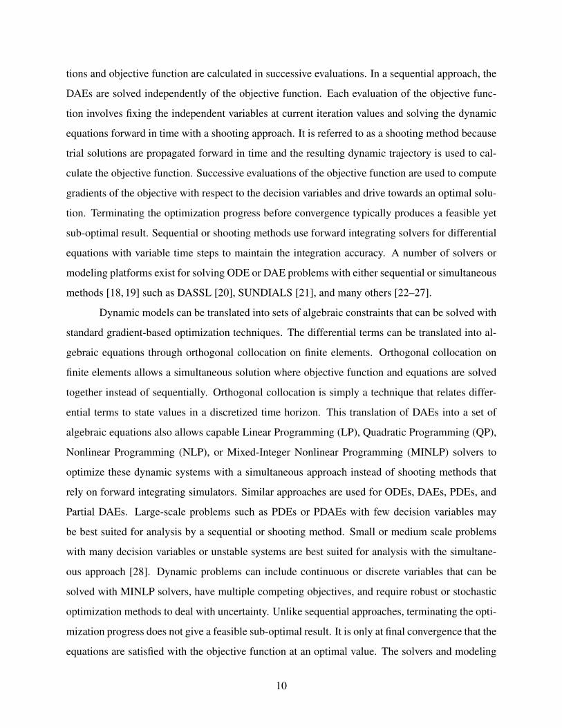
Figure 2.7: Lower block triangular form for pendulum data reconciliation
For initialization, a lower block triangular form of the index-3 DAE sparsity is used to
identify small subsets that can be solved independently as shown in Figure 2.7. Each subset of
equations is solved successively, leading to an initial solution with default parameters. An alter-
native approach is to pre-solve the system of equations with no degrees of freedom (DOF). This
simulation step is a simultaneous solution of variables and equations but with decision variables
fixed at nominal values. Table 2.4 presents results with the APOPT solver [33] while Table 2.5
gives results with the IPOPT solver [71]. With the APOPT solver, the initialization is not required
for the index-3 and index-2 models because the initial conditions as default variable values pro-
duce a sufficiently accurate guess to enable a successful solution. On the other hand, some cases
do benefit from the initialization strategy by decomposition as shown in Tables 2.4 and 2.5. These
results show that both the active-set (APOPT) and interior point (IPOPT) sequential quadratic pro-
gramming (SQP) methods benefit from initialization although the initialization time may increase
the total time for some model forms as shown in this particular case.
The subsequent examples demonstrate that performance improvements are often possi-
ble with initialization but for the pendulum case there is no CPU-time benefit when considering
the combined time of initialization and solution. The fastest solution for index-3 models is with
APOPT and no initialization in 15.09 sec. For index-2 models it is with IPOPT and no initializa-
tion in 1.40 sec. The combined time for index-1 models is fastest with IPOPT in 2.68 sec although
after initialization IPOPT solves the problem in 1.27 sec. Finally, for the index-0 (ODE) model, the
26

Table 2.4: Summary of Initialization Results with APOPT
DAEForm
Strategy Var Initialize Solution Total Iter
Index-3 Decompose 3401 2.31 sec 13.37 sec 15.68 sec 24Index-3 No DOF 3401 6.17 sec 13.72 sec 19.89 sec 24Index-3 No Init 3401 - 15.09 sec 15.09 sec 19Index-2 Decompose 3401 3.12 sec 1.78 sec 4.90 sec 6Index-2 No DOF 3401 5.81 sec 2.36 sec 8.17 sec 4Index-2 No Init 3401 - 6.46 sec 6.46 sec 8Index-1 Decompose 3401 30.8 sec 2.25 sec 33.1 sec 4Index-1 No DOF 3401 Failed - - -Index-1 No Init 3401 - Failed - -Index-0 Decompose 3601 37.5 sec 3.53 sec 41.0 sec 3Index-0 No DOF 3601 Failed - - -Index-0 No Init 3601 - Failed - -
Table 2.5: Summary of DAE Initialization Results with IPOPT
DAEForm
Strategy Var Initialize Solution Total Iter
Index-3 Decompose 3401 4.82 sec Failed - -Index-3 No DOF 3401 1.41 sec Failed - -Index-3 No Init 3401 - Failed - -Index-2 Decompose 3401 5.12 sec 0.93 sec 6.05 sec 17Index-2 No DOF 3401 1.28 sec 0.52 sec 1.80 sec 11Index-2 No Init 3401 - 1.40 sec 1.40 sec 28Index-1 Decompose 3401 44.1 sec 1.27 sec 45.4 sec 4Index-1 No DOF 3401 Failed - - -Index-1 No Init 3401 - 2.68 sec 2.68 sec 41Index-0 Decompose 3601 31.2 sec 1.29 sec 32.5 sec 20Index-0 No DOF 3601 Failed - - -Index-0 No Init 3601 - Failed - -
fastest combined solution is with IPOPT in 32.5 sec. With IPOPT, a solution is only possible with
initialization because the solver failed to find a solution within 100 iterations when the problem
was terminated.
27

2.4.2 Linear Initialization: CSTR Case Study
In linearized state-space form, it is generally easier to obtain an implicit solution to the
dynamic optimization problem. For small systems, it is possible to obtain an explicit solution to
MHE and MPC. The solutions with linearized models are then used to initialize the nonlinear case.
Prior work shows that initialization with linear or convex approximations to parameter estimation
problems improves the convergence properties of the nonlinear or possibly non-convex problems
[72]. A continuously stirred tank reactor (CSTR) with first order kinetics is a common benchmark
problem used in other studies to demonstrate estimation [73] and control [74] algorithms. Species
A and an energy balance equation for the CSTR in Figure 2.8 are shown in Equation 2.9. The
reactor is fed with chemical A and a diluent. The objective is to maintain temperature control
below 400 K in the reactor and the concentration of A below 0.2 mol/L.
Figure 2.8: Continuously Stirred Tank Reactor
VdCa
dt= q
(Ca f −Ca
)− k0exp
(− E
R T
)V Ca (2.9a)
ρVCpdTdt
= q(Tf −T
)+∆Hr k0exp
(− E
R T
)V Ca +UA(Tc−T ) (2.9b)
With an elevated jacket temperature, without a controller in place, the reactor experiences
temperature run-away as shown in Figure 2.9 due to the exothermic heat generation and exponen-
tial dependence on temperature. The exponential increase in temperature is also accompanied by
a decrease in concentration of species A. The uncontrolled reactor temperature violates the upper
limit on reactor temperature of 400 K. Solving the simulation case with zero degrees of freedom,
28

as shown above, helps develop a feasible solution for the problem. This feasible solution can then
be used to initialize the decision variables for the main nonlinear CSTR problem.
Figure 2.9: Uncontrolled linear and nonlinear response
A Nonlinear Model Predictive Controller (NMPC) is developed to reduce the concentration
of A below 0.1 mol/L and maintain the temperature between 375−380 K. A reference trajectory
with an `1-norm deadband [35] guides the approach to the desired setpoint as shown in Figure
2.10. The nonlinear MPC is initialized with a preliminary linear MPC solution (Equation 2.10b)
or through structural decomposition. This potential initialization strategy is to solve a lower block
triangular form of the nonlinear MPC to initialize the state and parameter values for a warm start
near the desired solution (see Figure 2.11).
dCadtdTdt
=
−( qV + k
)−k E
RT 2
∆HrkρCp
(− q
V −UA
ρCpV + ∆HrkρCp
ERT 2
)Ca
T
+ q
V 0 0
0 qV
UAρCpV
Ca,i
Ti
Tc
(2.10a)
[T]=[0 1
]Ca
T
+[0 0 0]
Ca,i
Ti
Tc
(2.10b)
29
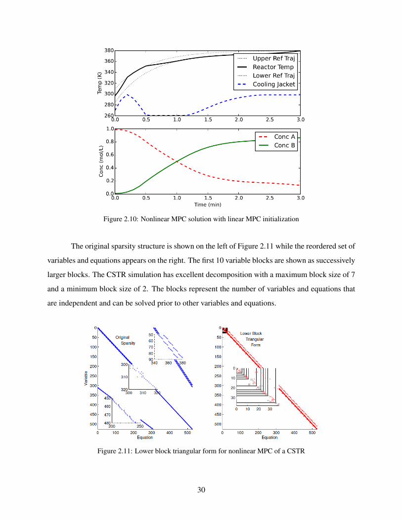
Figure 2.10: Nonlinear MPC solution with linear MPC initialization
The original sparsity structure is shown on the left of Figure 2.11 while the reordered set of
variables and equations appears on the right. The first 10 variable blocks are shown as successively
larger blocks. The CSTR simulation has excellent decomposition with a maximum block size of 7
and a minimum block size of 2. The blocks represent the number of variables and equations that
are independent and can be solved prior to other variables and equations.
Figure 2.11: Lower block triangular form for nonlinear MPC of a CSTR
30

Table 2.6: CSTR MPC comparison of linear pre-solve, block diagonal decomposition, and no initialization
Solver Strategy Var Initialize Solution Total IterAPOPT Decompose 1054 0.10 sec 0.51 sec 0.61 sec 13APOPT Linear 1054 0.17 sec 0.45 sec 0.62 sec 18APOPT No Init 1054 - 0.95 sec 0.95 sec 27IPOPT Decompose 1054 0.42 sec 0.64 sec 1.06 sec 40IPOPT Linear 1054 0.51 sec 2.01 sec 2.52 sec 119IPOPT No Init 1054 - 1.27 sec 1.27 sec 65SNOPT Decompose 1054 0.11 sec 0.37 sec 0.48 sec 23SNOPT Linear 1054 0.15 sec 2.78 sec 2.93 sec 108SNOPT No Init 1054 - Failed - -
Table 2.6 gives results for solvers APOPT [33], IPOPT [71], and SNOPT [75] with three
scenarios including decomposed solution initialization, linear pre-solve, and no initialization ex-
cept use of initial conditions. The fastest solution case is with a decomposition solution with
SNOPT with a total time of 0.48 sec. The nonlinear MPC case is initialized with only the initial
conditions that are propagated forward across the time horizon before solution begins. The best
solution time without initialization is with APOPT at 0.95 sec or twice the CPU time even when the
additional pre-solve decomposition time is included. For SNOPT, a solution is only possible with
initialization because the original problem fails to solve after 500 iterations. An important result
from this CSTR study is that initialization effectiveness is solver dependent but that an initialization
strategy tends to improve solution time for all solvers. At a future point, solvers may incorporate
initialization strategies that exploit the high degree of DAE problem structure to provide a feasible
starting point.
2.4.3 Tethered Aerial Pipeline Inspection: Initialization with Sequential Simulation
One of the limitations of small Unmanned Aerial Vehicles (UAV) is the limited range with
current battery technology and regulatory hurdles for autonomous and commercial flights in many
jurisdictions. One method to overcome both of these obstacles for infrastructure inspection is to
tether the aerial vehicle to a ground vehicle. The tether can provide a communication and power
conduit to the UAV to allow it to remain aloft indefinitely. The ground vehicle and aerial UAV
31

may be a fully automated system that is designed to regularly monitor infrastructure such as levee
systems, bridges, dams, pipelines, electrical transmission cables, and other large scale structures.
In this simulation, a UAV is tethered to an autonomous ground vehicle. As the ground
vehicle drives to the side of a pipeline, a multi-copter UAV hovers above the pipeline with an array
of cameras and leak detection sensors. The cable that connects the UAV to the ground robot is
specified to be 25 m in length. In this case the cable length is fixed although a retractable ground
vehicle-based or UAV-based cable is possible to adjust cable length and maintain cable tension.
Figure 2.12: Lower block triangular form for a tethered UAV
A simplified model of this multi-agent optimization problem consists of DAEs as shown
in [3] but with a fixed position for the ground robot instead of dynamic equations for the drogue.
The sparsity and structural decomposition are shown in Figure 2.12. The cable system dynamics
are modeled by discrete nodes at regularly spaced intervals along the cable. The elasticity of the
cable, cross-wind disturbances, movement of the aerial and ground robots all contribute to the
complex cable and UAV movement. The dynamics of the cable are important to plan a path for
the UAV that maintains a minimum tension on the cable to avoid excessive slack. A secondary
objective beyond maintaining tension limits is to fly along a corridor above the pipeline and keep
pace with the movement of the ground vehicle. For fixed wing vehicles, a minimum relative air
velocity is required to maintain lift on the vehicle. A minimum relative air velocity is enforced in
this simulation although not required by a multicopter platform.
32

Unique aspects of this example problem for DAE initialization are that it is an unstable
system, highly nonlinear, and has many decision variables. The optimizers plan a path for the
UAV by adjusting the acceleration of the UAV in north, east, and vertical directions. Acceleration
limits(
1 ms2
)are enforced to emulate responsive yet limited UAV capabilities. The optimizers seek
to maintain tension, elevation above pipeline, position over the pipeline, and air velocity to meet
monitoring objectives.
Figure 2.13: A simulated tethered UAV performs surveillance of a pipeline.
For this application, initialization steps are critical to first obtain a feasible and then optimal
solution. In this case, the initialization is accomplished with either the lower block triangular
solution or else with a single simulation with no degrees of freedom. The dynamic optimization
of 5,670 variables and 5,544 equations is solved in APMonitor (APOPT, IPOPT, and SNOPT
solvers) with a 2.4 GHz Intel i7-2760QM Processor. The results for this analysis are summarized
in Table 2.7. Without initialization, the solvers fail to find a solution with a maximum of 1,000
iterations and CPU time of 3,600 sec.
33

Table 2.7: Tethered UAV comparison of linear pre-solve, block diagonal decomposition, and no initialization
Solver Strategy Var Initialize Solution Total IterAPOPT Decompose 5670 3.1 sec 246.9 sec 250.0 sec 298IPOPT Decompose 5670 15.1 sec 47.2 sec 62.3 sec 255SNOPT Decompose 5670 3.2 sec 31.6 sec 34.8 sec 164APOPT No DOF 5670 2.6 sec 292.0 sec 294.6 sec 96IPOPT No DOF 5670 7.8 sec 61.7 sec 69.5 sec 158SNOPT No DOF 5670 4.4 sec 136.0 sec 140.4 sec 656APOPT No Init 5670 - Failed - 1,000IPOPT No Init 5670 - Failed - 1,000SNOPT No Init 5670 - Failed - 1,000
2.4.4 Smart Grid Energy System: Structural Decomposition
Cryogenic carbon capture (CCC) is a new technology for separation of CO2 from flue
gas. In this process, CO2 is separated by cooling the temperature to lower than the CO2 freezing
point. The main advantages of the CCC process are low energy consumption, fast response to load
changes, and energy storage capability. The latter advantage is critically important for grid stabil-
ity, especially in the face of a large penetration of renewable energy. Time-shifting the electricity
demand of the CCC process is a result of the energy storage capability that can positively influence
power grid stability. Integration of the CCC process with grid-scale power generation units includ-
ing coal, gas, and wind power units is detailed in Chapters 4 to 6. The integrated system without
energy storage is considered as an example case study for initialization purposes. A schematic
diagram of the integrated system is shown in Figure 2.14.
The refrigeration cycles in the CCC process and integration of the process with power gen-
eration units make it a complicated system where many of the variables are co-dependent. The
sparsity and structural decomposition of this system are shown in Figure 2.15. The model decom-
poses into 3072 separate blocks with the largest block at 14 variables and the smallest block at 1
variable. The independent blocks are, however, dependent on prior solutions of other independent
blocks.
The goal in this study is to maximize the operational profit of the integrated system. The
hybrid system is required to meet the total electricity demands of the CCC process and residential
area. In addition, the amount of the power produced should be controlled to avoid the excess power
34
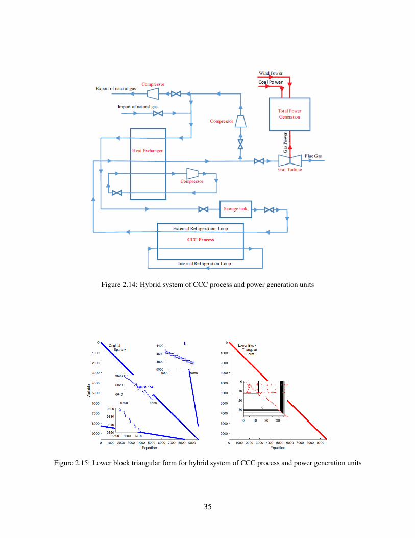
Figure 2.14: Hybrid system of CCC process and power generation units
Figure 2.15: Lower block triangular form for hybrid system of CCC process and power generation units
35

production. A dynamic optimization framework is used with a time horizon of 8 days and 1 hour
time increments are considered. Consideration of eight days as the simulation time ensures that the
results are not influenced by the initial and boundary conditions. The results for the three middle
days of interest are shown in Figure 2.16. The number of variables and equations are 15,552 and
14,784, respectively, leading to 768 decision variables. This is more than the decomposition case
(9,600 variables and equations) or the dynamic simulation case (7,488 variables and equations)
because of the additional equations and variables necessary to implement reference trajectories and
manipulated variable tuning. The 768 decision variables are the amount of coal and natural gas
combusted for power production and the amount of natural gas imported to and exported from the
plant at each time step. The model is implemented in APMonitor and is solved using the APOPT
solver. The optimization problem is solved on a Dell R815 Server with an AMD Opteron Processor
6276 (2.3 GHz).
Without initialization of the problem, the solver fails to obtain a solution with a maximum
of 400 iterations and CPU time of 14 hr. Several initialization strategies are used to obtain a
feasible solution: (1) Nominal values are assigned for the decision variables and the problem and
objective equations are solved with equal numbers of variables and equations (square problem),
(2) the square problem is solved by using the structural decomposition of the equations, (3) restart
from simultaneous dynamic simulation with all degrees of freedom fixed at specified values, and
(4) restart from sequential dynamic simulation where initialization is accomplished by solving
the square problem in a sequential time-step approach. With the strategies described above, the
decision variables are initialized from the simulation case and the optimization case is solved. In
this stage, decision variables are obtained by the optimizer. The combined CPU times for both the
initialization and final solution for each case are summarized in Table 2.8. Results for IPOPT and
SNOPT are not reported because the solvers failed for all cases. The computational time of each
initialization step is reported in seconds as well as the total computational time in hours.
Of all of the cases, only case 4 had a feasible solution after the initialization step. The other
cases also produced a solution but the solver was not able to find feasible values to satisfy all of the
equations within a specified convergence tolerance. Interestingly, even starting from the infeasible
solution helped the optimization case to find a successful solution. As it is seen from Table 2.8,
initializing the optimization problem with a sequential dynamic solution of the square problem
36

Figure 2.16: Power and demand profiles for the hybrid system of CCC process and power generation units
Table 2.8: Computation time for hybrid system of a CCC process and power generation units
Case Strategy Var Initialize Total Iter0 No Initialization 15,552 Skipped Failed 4001 Simultaneous simulation with
objective equations9,600 57.5 sec 5.56 hr 214
2 Structural decomposition asshown in Figure 2.15
9,600 25.6 sec 5.55 hr 214
3 Simultaneous simulationwithout objective equations
7,488 25.4 sec 5.54 hr 214
4 Sequential simulation initial-ization
7,488 2.5 sec 2.67 hr 137
has the least amount of computation time while the other three cases take approximately the same
amount of time to achieve a successful solution. The result of the optimization case is shown in
37

Figure 2.16, where total electricity demand of the hybrid system is met through a combination of
the coal, gas, and wind power.
2.5 Conclusions
A contribution of this dissertation is a strategy for improved initialization of dynamic sys-
tems. Techniques include structural decomposition, pre-solve with linear models, and initializa-
tion with no degrees of freedom. The dynamic models are often hybrid systems of fundamental
relationships and empirical parameters that can be adjusted to fit model predictions to data or opti-
mized over a time horizon. The discretized sparse structure is restructured to identify independent
sets of variables and equations that can be solved successively and independently. Higher index
DAEs, integral equations, and higher order derivatives fit into a general framework for addressing
large-scale optimization of dynamic systems. Several case studies motivate the use of initializa-
tion to improve solution time and enable successful solutions. While all initialization strategies
used in this analysis helped the convergence of the problem, finding the best approach for different
problems is the focus of future work.
38

CHAPTER 3. FRAMEWORK FOR DYNAMIC PARAMETER ESTIMATION ANDOPTIMIZATION
3.1 Introduction
There are approximately 40,000 distillation columns in the US that are used to separate
chemical compounds based on vapor pressure differences in industries ranging from oil and gas to
pharmaceuticals. These separation columns consume 6% of the yearly US energy demand [76].
While many of the large production facilities use continuous processes, specialty and smaller-use
items are often processed in batch columns [77–79]. Continuous distillation columns have been
the focus of optimization work since the first column was built, but the transient nature of batch
columns has caused many to remain unoptimized. The transient nature of the market for these
specialty items has further hindered the optimization of batch columns [78]. As a result, little re-
search on batch column optimization is available in the literature before 1980 [80–83]. Work on
batch columns has increased in the last 30 years as computers have become more sophisticated,
and several studies have considered both advanced solving techniques and advanced column con-
figurations [84–98]. Terwiesch, et al. [99] and Kim and Diwekar [100] provide a detailed history
of the subject and a description of current batch distillation modeling and optimization methods.
The optimization of the batch columns can be subdivided into optimal design problems
and optimal control problems. Optimal design problems generally deal with column configuration,
while optimal control problems deal with column operation. These ideas are summarized well in
separations textbooks such as Diwekar [85], Stichlmair and Fair [101] and Doherty and Malone
[102] and will therefore not be discussed further here. Research studies on this subject follow
the same general outline as presented in the textbooks [78, 103]. The models developed for batch
column optimization generally fall into two categories: first-principles models and shortcut or
simple models.
39

First-principles models are those with governing mass and energy balance equations, de-
tailed thermodynamics, tray dynamics, system non-idealities and variable flow rates [104–107].
These models are theoretically more accurate than shortcut methods, but they are only as accurate
as the thermodynamic and physical property models they use [78]. The use of these models has
been limited due to high computational costs. Several studies have been conducted using first-
principles models and advanced solving techniques to reduce computational cost [57, 108–113].
While these models accomplish the goal of reducing computational load, they are generally still
slower than shortcut models. In addition, the lack of experimental data for batch columns makes
it difficult to determine how much accuracy is lost when going from first-principles to lower-order
(first-principles model with advanced or simplified numerical methods) to shortcut models [114].
The second class of models, shortcut models, has received far greater attention. These
models contain less physics and are generally used for ballpark estimates and comparative studies.
A typical set of assumptions for these models is as follows: constant boil-up rate, no external
heat loss, ideal stages, constant relative volatility, constant molar overflow, total condenser without
subcooling and no column holdup [103, 106, 115–117]. More recent shortcut models have kept
most of the same assumptions while accounting for column dynamics using a non-zero column
holdup [111, 114]. The primary purpose of these models is to create an accurate, computationally
fast simulation for use in design and control of batch columns. While these models achieve the
reduction in computational load, the lack of experimental data makes it difficult to determine the
accuracy of these models [114]. The assumptions made in these models limit their use to ideal
systems.
The gap between first-principles models and shortcut models is large. First-principles mod-
els can provide predictions for many systems but require thermodynamic and physical property
models as inputs, while the assumptions in shortcut models make them applicable only to a small
class of relatively ideal systems. In this work, a method is proposed for developing shortcut models
with relaxed assumptions. The method is based on fitting parameters in place of simplifying as-
sumptions to include system non-idealities without solving the first-principles equations. Solving
for the fitting parameters requires extensive experimental data whereas first-principles models typ-
ically need less data, being based on fundamental correlations. Dynamic parameter estimation can
be used to reduce the experimental load. The case study presented in this work required only one
40

Figure 3.1: Overview of methodology for batch column optimization with novel contributions underlined
experiment to determine model parameters. As with any model containing fitting parameters, there
is concern over the accuracy of the parameters. By using nonlinear statistics [118] and a model
sensitivity analysis [119], it is possible to determine how many parameters can be estimated from
the collected data and the acceptable range for those parameters. These steps are shown in Figure
3.1 (also shown in Chapter 1). Underlined elements of the methodology in Figure 3.1 indicate the
new approach to batch separation systems.
The well-known methodology shown in Figure 3.1 is applied to an experimental case study.
The methodology includes the use of `1-norm dynamic parameter estimation, nonlinear statistics
[118,120], and a model parameter sensitivity analysis [119]. These techniques are applied together
to a batch distillation column in a holistic approach to dynamic optimization. Models developed
using this method account for system non-idealities not seen in typical shortcut models without
sacrificing computational speed.
41

It should be emphasized that the dynamic parameter estimation, nonlinear statistics, and
control frameworks developed for the batch distillation column are applicable more generally to
complex dynamic systems. The general frameworks used for modeling, estimation, and control of
this problem are discussed in Section 2.2. In Section 3.1.1, the general equations used to represent
the nonlinear statistics and sensitivity analysis are overviewed.
3.1.1 Confidence Intervals and Sensitivity Analysis
Reliability of the parameters is investigated by implementing an approximate nonlinear
confidence interval calculation [118]. Non-linear confidence intervals can be found by solving
Equation 3.1 for the sets of parameters that make up the joint confidence region [121], then ex-
tracting the upper and lower bounds of that region in each dimension.
J(θ)− J(θ ∗)J(θ ∗)
≤ pn− p
Fn,n−p,1−α (3.1)
In Equation 3.1, J(θ) is the error between the measurements and the model prediction at a
value θ of the parameters, J(θ ∗) is the error between the measurements and the model prediction
at the best estimates of the parameters (θ ∗), p is the number of parameters in the model, n is
the number of data points, and Fn,n−p,1−α is the F-statistic at n and n− p degrees of freedom
with a confidence level of 1−α . The squared error objective is the only form of the nonlinear
confidence interval that has a theoretical foundation. This is because the F-statistic used to define
the confidence region is a ratio of χ2 distributions that compares the equivalence of two sets of
experimental results. The χ2 distributions are intended for least square objectives instead of `1-
norm objectives. According to the author’s knowledge, an equivalent F-statistic for nonlinear
confidence intervals and the `1-norm has not been derived. A nonlinear confidence interval for
`1-norm objectives based on the F-statistic is future work.
It is also desirable to determine the number of parameters that can be estimated or are
observable given a particular model form and set of data. Large confidence intervals signal that a
particular parameter may not be observable or that the effect of that parameter may be co-linearly
dependent with other parameters. A well-known systematic analysis is used to determine which
parameters can be estimated and rank the parameters in terms of the ability of a particular parameter
42

to improve a particular model estimate [119, 122]. This procedure is accomplished in 3 steps: (1)
efficient computation of the sensitivities, (2) scaling of the dynamic parameter sensitivities, and (3)
singular value decomposition of the scaled sensitivity matrix to reveal an optimal parameter space
transformation.
The first step in performing the parameter analysis is to compute the state dependencies
to changes in the parameters. This can be accomplished with a variety of methods. One such
method is to compute a finite difference sensitivity of the parameters with a series of perturbed
simulations [123, 124]. A second method is to augment the model with adjoint equations that
compute sensitivities simultaneously with the model predictions [125]. A third method is a post-
processing method with time-discretized solutions to differential equation models [3, 8, 126]. This
post-processing method involves efficient solutions to a linear system of equations, especially over
other methods for large-scale and sparse systems [17].
The sensitivity is computed from time-discretized models that are solved by nonlinear pro-
gramming solvers. At the solution, exact first derivatives of the equations with respect to variables
are available through automatic differentiation. These derivatives are available with respect to the
states (∇ fx(x,θ)) and parameters (∇ fp(x,θ)). For the objective function, objective gradients are
computed with respect to states (∇Jx(x,θ)) and parameters (∇Jθ (x,θ)). Sparsity in those matrices
is exploited to improve computational performance, especially for large-scale systems. Sensitiv-
ities are computed by solving a set of linear equations as shown in Equation 3.2 with parameter
values fixed at θ and variable solution x as nominal values.∇x f (x, θ) ∇θ f (x, θ) 0
∇xJ(x,θ) ∇θ J(x,θ) −1
0 I 0
∇θ x
∇θ θ
∇θ J(θ)
=
0
∆θi = 1
0
(3.2)
To further improve the efficiency of this implementation, an LU factorization of the left
hand side (LHS) mass matrix is computed. This LU factorization is preserved for successive
solutions of the different right hand side (RHS) vectors because the LHS does not change and suc-
cessive sparse back-solves are computationally efficient in comparison with the LU factorization.
Each matrix inversion computes the sensitivity of the states to a particular parameter. Each param-
eter is successively set equal to a change of ∆θi = 1. All other elements of the vector on the RHS
43

are set to 0. The solution to this matrix inversion computes the sensitivity of all variables in the
time horizon with respect to a particular parameter S = (∇θ x). It also computes the sensitivity of
the objective function with respect to the parameters(∇θ J(θ)
).
To summarize the sensitivity analysis, an efficient method is presented to compute sensitiv-
ities as a post processing step that is efficient even for large-scale and sparse systems. The sensitiv-
ity matrix is decomposed into singular values and eigenvectors that give the relative magnitude and
linear combination of parameters that are orthogonal. In this study, the transformed parameters are
not estimated directly but instead used as an advisory tool to determine which parameters and how
many can be estimated.
3.2 Dynamic Estimation and Optimization for a Batch Distillation Column
This established methodology is demonstrated for the first time on a binary batch distil-
lation column. While the methods are not new, the application to this specific column is novel
and gives experimental insight on issues encountered when applying dynamic optimization on ap-
plications that share common features. This section is subdivided into a brief discussion of the
apparatus and experimental procedure, parameter estimation and validation, and model optimiza-
tion and validation.
3.2.1 Apparatus and Experimental Procedure
A 38 tray, 2 inch, vacuum-jacketed and silvered Oldershaw column is used to collect all
experimental data (see Figure 3.2). Cooling water supplies the energy sink for the total condenser
at the top of the column. A 600 W reboiler heater is the only source of energy input. Reflux
ratio is set using a swinging bucket and can be changed as frequently as every 5 minutes. The
instantaneous distillate composition is determined using the refractive index of the solution and the
total distillate collected is determined via a graduated cylinder. Cumulative distillate composition
can be measured and inferred using the instantaneous compositions and a mass balance. The
instantaneous distillate composition can be measured every 5 minutes. The reboiler is initially
charged with 1.5 L of a 50/50 wt% mixture of methanol and ethanol for each run, with the goal
being a product of 99 mol% methanol.
44

Figure 3.2: Apparatus used for the experiments
The non-optimized base case experiment consists of running the column at total reflux for
30 minutes, then setting the reflux ratio to a constant value, usually somewhere between 3 and 5,
and letting the column run until the cumulative overhead composition reaches 99 mol% methanol.
The collection time usually lasts 60 to 90 minutes, depending on the reflux ratio. The instantaneous
and cumulative compositions for a typical run, as well as the amount of product collected, can be
seen in Figures 3.3a and 3.3b, respectively. In this case, running the column at total reflux for 30
minutes, then using a constant reflux ratio of 4 for the next 90 minutes resulted in 13.7 moles of 99
mol% methanol.
45

(a) Instantaneous and cumulative product mole frac-tion (b) Methanol production
Figure 3.3: Non-optimized base case where the final required purity (> 99 mol% ethanol) is not met
3.2.2 Equations for the Simplified Process Model
Distillation is an inherently complex process involving mass and energy transfer, thermo-
dynamics, and often reaction kinetics. Models that describe these phenomena do not have to be
complex, however. The model developed here is used to describe the separation of a 50/50 wt%
mixture of methanol and ethanol, and is simple by design to illustrate this point.
The VLE model used here is found in the CHEMCAD database [127] and is shown in
Equation 3.3:
y∗n =−2.016x4n +0.6861x3
n−1.206x2n +1.721xn +0.0003984 (3.3)
where xn is the liquid mole fraction of methanol and y∗n is the vapor mole fraction of methanol
in equilibrium with the liquid. The subscript n denotes the stage for which the mole fraction is
being calculated. The temperature difference across the column is not considered for the simpli-
fied model developed in this Section; however, the impact of temperature change throughout the
column is considered in the model developed in Section 3.2.3. An adjustment to the equilibrium
vapor mole fraction is used because equilibrium is not often achieved during column operation.
This adjustment is in the form of a Murphree efficiency and is shown in Equation 3.4:
yn = yn+1−EMV (yn+1− y∗n) (3.4)
46

where yn is the actual mole fraction and EMV is the efficiency. The efficiency is a fitting parameter
used to account for system non-idealities and is found using the data collected as part of this work.
The liquid mole fraction for each stage is found by performing a material balance at each
stage, n, as shown by Equation 3.5 where V is the vapor flow through the column, L is the liquid
return flow, and Ntray is the number of moles of liquid on the stage. The number of moles and the
composition in the reboiler (Nreb and xreb) change with time and are represented by Equations 3.6
- 3.7. The number of moles in the condenser (Ncond) is assumed constant while the composition
of the condenser (xcond) varies throughout the run (see Equation 3.8). Variation of the number of
moles and composition of the product with time are represented by Equations 3.9 and 3.10. The
liquid holdup for the condenser and trays are also design variables and are described in Equations
3.11 and 3.12, where ftray and fcond are the fitting parameters representing the fraction of the
initial reboiler charge on each tray and in the condenser, respectively. The tray holdup is assumed
constant across all stages. The stages are numbered from 1 to 40 with the top being 1 (condenser).
dxn
dt=
L(xn−1− xn)−V (yn− yn+1)
Ntray(3.5)
xrebdNreb
dt+Nreb
dxreb
dt= Lx39−V yreb (3.6)
dNreb
dt= L−V (3.7)
Nconddxcond
dt=V (y2− xcond) (3.8)
dnp
dt= D (3.9)
xpdnp
dt+np
dxp
dt= D xcond (3.10)
Ncond = Nreb.init fcond (3.11)
47

Ntray = Nreb.init ftray (3.12)
The vapor flow rate is found using the energy balance shown in Equation 3.13:
V =hdot h f
Hvap(3.13)
where hdot is the heat input from the heater, Hvap is the heat of vaporization for the methanol/ethanol
system, and h f is a fitting parameter representing the heating efficiency. The heat of vaporization
is approximated as a weighted average of the pure component heats of vaporization obtained from
the DIPPR Database [128]. The liquid flow rate, the reflux ratio, and the distillate rate are found
using an overall mass balance and the definition of the reflux ratio, shown in Equations 3.14 and
3.15, respectively:
V = L+D (3.14)
R =LD
(3.15)
where R is the reflux ratio and D is the distillate rate. Constant molar overflow is assumed through-
out the model and applies to the equations shown above.
3.2.3 Equations for the Detailed Process Model
A more detailed (although not completely from first-principles) model [129] with energy
balance equations validates the simplified model developed in Section 3.2.2. A similar notation as
the simplified model is used for the detailed model with a distinction in the stage number in which
the material and energy balances are developed. Vapor and liquid leaving each stage are noted
as Vn and Ln, respectively. The equations used in the detailed model are based on the following
assumptions:
• constant molar hold up for the condenser and trays
• fast heat transfer throughout the column
• liquid temperature on each tray at the mixture bubble point
48

• vapor liquid equilibrium relationships based on temperature dependent vapor pressures
• pressure drop across each tray is 1 mmHg = ∆P
• temperature dependent density, heat capacity, vapor pressure, and heat of vaporization
The overall and component mole balances as well as the energy balance equation for a
control volume over the condenser and accumulator lead to Equations 3.16 to 3.19.
V2 = L1 +D (3.16)
L1 = R D (3.17)
Nconddxcond
dt=V2 y2− (L1 +D) xcond (3.18)
Qcond =V2 hV2− (L1 +D) hL1 (3.19)
A component and overall mole balance over the trays result in Equations 3.20 and 3.21.
Equation 3.22 also represents an energy balance for each tray in the column.
Ntraydxn
dt= Ln−1 xn−1−Ln xn +Vn+1 yn+1−Vn yn (3.20)
0 =Vn+1−Vn +Ln−1−Ln (3.21)
Vn+1 (hVn+1−hLn) =Vn (hVn−hLn)−Ln−1 (hLn−1−hLn) (3.22)
A component mole balance and the associated energy balance equation for the reboiler are
presented by Equations 3.24 and Equation 3.25. The reboiler heating rate, Qreb, is 600 W to drive
the separation together with the cooling of the condenser, Qcond . The overall mole balance for this
model is calculated from Equation 3.23.
49

dNreb
dt=−D (3.23)
xrebdNreb
dt+Nreb
dxreb
dt= L39 x39−V40 yreb (3.24)
Qreb h f =V40 (hV40−hL40)−L39 (hL39−hL40) (3.25)
Accumulation of product and the change in composition of the product with respect to
changes in product moles are shown in Equations 3.9 and 3.10. The enthalpy of mixture for
both liquid and gas phases is a mole average of the enthalpy of each component. Enthalpy of
each component is obtained by integrating the heat capacity for liquid and adding the heat of
vaporization for vapor. The temperature profile in the column is also a function of the equilibrium
composition of each stage. The relationship between temperature and liquid composition of each
stage is based on vapor pressure and the pressure on each tray (Pn) as shown in 3.26 with ns = 2.
P1 = 0.86 atm (Ambient Pressure in Provo, UT) (3.26a)
Pn = Pn−1−∆P (3.26b)
Pn =ns
∑i=1
γi xi Psati (Ti) (3.26c)
The vapor composition at each tray is determined by the vapor liquid equilibrium correla-
tion shown in Equation 3.27 and is combined with the previous Equation 3.4 to relate the equilib-
rium composition (y∗n) to the actual tray composition (yn) based on the Murphree efficiency.
y∗n Pn = γ xn Psatn (Tn) (3.27)
A full listing of the model equations, data, and Python source code is given in Appendix
A. The more sophisticated model demonstrates that the simpler and less rigorous model is able
to adequately predict the batch column performance for the purpose of optimization. The model
validation is shown in the subsequent section.
50

3.2.4 Model Validation
Model validation is accomplished through dynamic parameter estimation. The parameter
estimation experiment was similar to a doublet test, with reflux ratios set to 3.5, 1, 7 and 3.5. The
column was allowed to come to steady state at infinite reflux before starting data collection; the
reflux ratio was adjusted every 15 minutes thereafter. The parameters found by fitting the model
with experimental data are heater efficiency(h f), vaporization efficiency (EMV ), condenser molar
holdup as a fraction of initial reboiler charge ( fcond), and tray molar holdup as a fraction of initial
reboiler charge ( ftray). The parameter best estimates are shown in Table 3.1.
Table 3.1: Confidence interval calculation for the four parameter case
Parameter Best Estimate Upper 95% CI Lower 95% CIh f 0.719 0.799 0.639
EMV 0.691 2.420 0fcond 0.029 0.254 0ftray 5.077e-4 0.142 0
The instantaneous distillate composition from the experimental run and the associated sim-
plified and detailed model predictions using optimized parameters are shown in Figure (3.4a). The
maximum error between the simplified model predictions and the experimental values is 10%. The
maximum error between the more detailed model and experimental composition data is 4.8% for
the `1-norm objective and 5.3% for the squared error objective. Cumulative methanol production
is shown in Figure 3.4b. The error between model and prediction is almost non-existent using
both an `1-norm or squared error objective. The simplified model parameter estimation has 3,510
equations with the squared error objective and 3,780 equations with the `1-norm objective and
requires less than 10 CPU seconds to solve. The more detailed model parameter estimation has
11,644 equations with the squared error objective and 11,972 equations with the `1-norm objective
and requires 89.4 (`1-norm) and 53.1 (squared error) CPU seconds to solve. All calculations are
performed on a Intel Core i7-2760QM CPU operating at 2.4 GHz with the APOPT solver. Because
the simplified model produces similar results to the detailed model and solves sufficiently fast for
online real-time optimization, it is selected for the batch column optimization.
51

(a) Instantaneous distillate composition (b) Methanol production
Figure 3.4: Model validation for initial parameter estimation
(a) Instantaneous distillate composition (b) Methanol production
Figure 3.5: Insensitivity of the `1-norm estimation to outliers compared to the squared error objective
If artificial outliers are introduced in both the composition (80 mol% ethanol at t = 10 min
and t = 50 min) and cumulative production (15 moles at t = 30 min and t = 50 min), the squared
error predictions deviate while the `1-norm estimates do not (see Figure 3.5). This is because
the `1-norm is less sensitive to outliers and results in better predictions. In this comparison, the
same model and initial values are used to represent the governing equations of the distillation
column while the objective functions for error minimization differ, as described by [35]. While
this particular example did not include significant outliers, many industrial applications of batch
distillation may have instruments that report values with drift, noise, or outliers [130]. While gross
error detection can resolve many of these data quality issues, it is also desirable to have estimation
methods that are less sensitive to bad data as shown in this example.
52

3.2.5 Testing the Reliability of the Estimated Parameters
Nonlinear confidence intervals are calculated for four potential parameters. Confidence re-
gions are typically reported as upper and lower limits on a particular parameter. This work extends
the nonlinear confidence region to multivariate analysis that improve co-linearity assessment for
batch distillation processes beyond a singular value decomposition or linear analysis. However, a
look at the confidence interval for each individual parameter is useful to illustrate the procedure
for model validation. A wide confidence interval suggests that there is insufficient structure in the
model (observability) to determine the parameters from available measurements. Another insight
that is gained from the confidence intervals is a test of the data diversity that leads to tight confi-
dence regions. A tighter confidence region implies that a smaller deviation of the parameter from
an optimal value is not statistically likely given a set of data to which the model is reconciled.
Table 3.1 shows the expected value and 95% confidence interval for each parameter. As seen in the
table, the interval for heater efficiency is narrow and in the range of values expected for a heater.
The intervals for the other three parameters are large enough to include zero and the interval for
vapor efficiency includes physically impossible values. Although the fit between model and data
is excellent there are large parameter confidence intervals. One possible explanation for the large
intervals is that the model is over-parameterized and thus has too many degrees of freedom. Thus,
a sensitivity analysis is implemented to investigate the correct parameterization of the model.
The scaled sensitivity is shown graphically in Figure 3.6. The sensitivity is scaled by
solution values as Si, j =(∇θ jxi
)θixi
to show relative effects with a unitless transformation. The
scaling is applied with parameters θ and variables x at solution values. One clear result from this
sensitivity study is that the total production (np) is dependent on the heat input to the batch column
and that other parameters have little effect on the total production. As expected, a higher heating
rate (h f ) vaporizes additional liquid and increases the flow to the condenser. With a specified reflux
rate, the total production rate increases proportionally. In other words, a 1% increase in heating
produces 1% additional product. This scaled sensitivity is shown as a value of 1.0 in the top subplot
of Figure 3.6. The sensitivities of instantaneous product composition to the parameters are nearly
co-linear as seen by the bottom subplot of Figure 3.6. For example, heater efficiency(h f)
and tray
holdup fraction ( ftray) can be increased and decreased, respectively, to produce nearly the same
final answer. Other parameters also show a high degree of co-linearity.
53

Figure 3.6: Scaled variable sensitivities to the parameters
While sensitivity plots such as Figure 3.6 are instructive, it can be difficult for large-scale
systems to detect co-linearity or the number and selection of parameters that can be estimated from
the data. An alternative way to show the same information is to decompose the sensitivity matrix
with a singular value decomposition to reveal magnitudes of singular values (relative importance
of transformed linear combinations of parameters) and eigenvectors (orthogonal vectors for the
parameter space transformation). The singular value decomposition is applied to the dynamic
sensitivity analysis to show that there is one principle parameter(h f)
that can be used to match
production data (np) as shown in Figure 3.7.
In this application, the parameter h f is principally used to match np. For selecting a next
parameter, ftray or EMV are feasible candidates with similar effect on the model. Estimating a third
parameter is likely not needed as seen by the magnitude of the singular values. The singular value
analysis gives a linear combination of the parameters estimated in transformed parameter space as
given by the eigenvectors.
This analysis is useful even for the non-transformed parameter estimation where the param-
eter estimates have physical meaning and constraints are enforced to reflect physical realism. For
example, in the case of h f , a value greater than 1.0 is not likely because it represents the fraction
54

Figure 3.7: Magnitude of singular values from singular value decomposition reveals independent linearcombinations of parameters to reconcile data
of reboiler heater duty that enters the liquid. It is expected that some of the heat escapes due to
lack of insulation or conduction. In transformed space, the physical connection to the parameters
is lost.
As mentioned, ftray and EMV have a similar effect on the model. In this study, EMV is
selected as the second parameter. It was therefore determined to first solve for all four parame-
ters using `1-norm analysis, then fix both holdups and re-solve for the heater efficiency and the
vaporization efficiency. The resulting confidence region and parameter best estimates are shown in
Figure 3.8.
With only two parameters, the confidence regions are able to be graphically visualized.
Instead of confidence intervals with lower and upper bounds, the 95% confidence region is given
by any point within the area on the contour plot that falls within the boundary. Both the `1-
norm and squared error objectives are included in this plot to demonstrate that slightly different
optimal solutions and confidence regions are reported for differing objectives that align model
and measured values. One notable issue is that the objective function is relatively insensitive to
vapor efficiency (EMV ), especially as the vapor efficiency is above 0.4. The 95% confidence region
suggests that values between 0.37 and 1.0 are valid parameter estimates for EMV and that only one
parameter is required for parameter estimation. The objective function is very sensitive to heater
efficiency(h f)
but not to EMV . One possible explanation for this is that this is a high purity column
55

Figure 3.8: Contour and surface plots of the objective function value for values of heater efficiency (h f ) andvapor efficiency (EMV ). The 95% confidence interval for the `1-norm is not correct (future work) and theconfidence interval for the squared error is an approximation.
where a difference of 0.01 in the mole fraction is of approximate equal importance to about 1.0
mole of production. Although the objective is scaled to account for this discrepancy, parameters
such as h f greatly influence both the predicted moles produced and the product composition. The
additional parameter EMV is required to achieve an acceptable fit for product composition although
it is less influential than the value of h f . The objective function contours confirm the observations
from the sensitivity analysis and singular value decomposition shown previously in Figures 3.6
and 3.7. The fit to the parameter estimation experiment is shown in Figures 3.9a and 3.9b. With
the model sufficiently validated, the next step is to optimize the column control scheme.
3.2.6 Model Optimization and Validation
The objective in this case study is to maximize the amount of methanol produced in the
column during a 90 minute run. The non-optimized base case production over a 90 minute run is
9.5 moles of 99.2 mol% methanol at a constant reflux ratio of 4 (see Section 3.2.1). The design
56

(a) Instantaneous distillate composition (b) Methanol production
Figure 3.9: Model validation for final parameter estimates
variable in this study is reflux ratio, with the option to change the reflux ratio every 5 minutes.
The control scheme for the optimized run is shown in Figure 3.10; the base case profile is shown
for comparison purposes. The optimized reflux ratio scheme starts low before increasing in a
nominally linear pattern. This is done to take advantage of the initially high concentration of
methanol in the condenser after the startup period.
Figure 3.10: Reflux ratio for optimized control scheme compared to the non-optimized base case
The cumulative composition and total production are shown in Figure 3.11a and Fig-
ure 3.11b, respectively, with parameter values of h f = 0.8, EMV = 0.37, ftray = 0.0009, and
57

fcond = 0.006. Also shown in the figures are the model predictions and the non-optimized base
case results. The optimized control scheme resulted in 10.8 moles of 99.8 mol% methanol. This
change represents a 14% increase in column production over the base case. Given the high concen-
tration, it is possible to collect more product throughout the optimized run and still meet the purity
specification. However, given the error associated with experimental measurements, the prediction
was left at a slightly conservative estimate to ensure the purity specification was achieved. The suc-
cess of this effort is seen in the fact that the error bars on the optimized composition measurements
stay above the purity requirement while those for the non-optimized base case do not.
(a) Cumulative composition (b) Methanol production
Figure 3.11: Optimized control scheme compared to the non-optimized base case and to the model predic-tion
Also seen in the figures are the model predictions. The model predicts 9.75 moles of 99.0
mol% methanol will be produced during the run. The difference between model prediction and
experiment is 10% and 0.8% for overall production and product composition, respectively. The
agreement between model and experiment is excellent and reflects the work done to validate the
model.
3.3 Conclusions
Models of batch distillation are typically either first-principles and computationally expen-
sive or simple and valid for ideal systems. In this work, a well-known methodology for parameter
estimation, uncertainty quantification, and dynamic optimization is used to develop a simplified
model for optimization of a batch distillation column. This methodology uses experimental data
58

to solve for model fitting parameters and validates the results with nonlinear confidence intervals.
This allows the models to include system non-idealities and be applicable for real-time analysis.
This is accomplished using dynamic data with `1-norm error minimization. A dynamic sensitivity
analysis reduces batch experimental data requirements by determining a priori which parameters
can be estimated. Nonlinear statistics are applied to quantify a posteriori the accuracy of those
same parameters. The results from the simplified model also agree with a first-principles model
but the simplified model solves 5-10 times faster than a first-principles model. While the methodol-
ogy is not novel, the application to this specific case study with experimental data is demonstrated
for the first time with insight into practical implications of working with real data.
The case study involves optimizing the control scheme for an existing batch column. A
38 tray, 2 inch, vacuum-jacketed and silvered Oldershaw batch distillation column was used to
collect experimental data. One experiment was performed to collect data for model validation and
another experiment was performed to validate the optimized control scheme. The optimized con-
trol scheme resulted in a 14% production increase over the base case while still meeting the purity
requirements. The model predictions for the optimized run are within 10% of the experimental
data.
59

CHAPTER 4. HYBRID SYSTEM OF CRYOGENIC CARBON CAPTURE AND POWERGENERATION UNITS
4.1 Introduction
Electricity transmission is one of the main forms of energy delivery today. According to
the International Energy Agency (IEA) [131], electricity transmits roughly 33% of the total energy
worldwide. Over eighty percent of this electricity is generated from non-renewable sources [132].
This makes the power sector one of the main sources of CO2 emission. The International Energy
Agency (IEA) estimated 42% of the 2012 global CO2 emissions are derived from power and heat
production [133]. There is nearly universal agreement among climatologists that anthropomorphic
CO2 and other greenhouse gases are the main causes of global warming [134]. The US and other
developed nations have reduced CO2 emissions in recent years through a combination of events,
including a global recession, transformation from coal to natural gas in new power generation
systems, increased automobile efficiency, and decreased miles driven [134, 135]. Furthermore, in-
terest in renewable energy sources like solar and wind power continues to increase which further
helps reduce the CO2 emissions. However, many renewable energy supplies are intermittent and
have capacity factors that are small compared to thermal power generation units. Therefore, be-
cause a one megawatt (MW ) wind or solar power unit cannot replace a 1 MW thermal power unit,
wind or solar power units must be integrated with thermal power units to develop a reliable power
generation system.
There is a wide body of research on integrated power generation systems that include both
thermal and renewable power plants. Goransson et al. [136] presented a model to investigate the ef-
fect of large-scale wind and thermal power integration. The purpose of the study was to investigate
the impact of wind power generation on the production strategies of thermal power production sys-
tems. They also considered the startup and turn down performance of the thermal units. However,
spinning reserves must often be on standby due to the limited rate of startup and the possibility
60

of decrease from an intermittent supply. Delarue et al. [137] studied the impact of wind power
generation on the cost associated with electricity generation, fuel, and CO2 emission. They con-
sidered the unpredictability of wind speed forecast and proposed a wind forecasting method. The
power plant was scheduled over a 24 hour horizon with forecasted wind power data to meet the
demand with minimal cost. Hu et al. [138] developed a Solar Aided Power Generation (SAPG)
system, using the traditional Rankine power cycle and solar heating. They concluded that SAPG
is more efficient than both the solar thermal power systems and the conventional fuel-fired power
cycles. Manenti et al. [139] developed a dynamic model for solar power plants with storage. The
dynamic simulation optimized power generation and improved the net income of a concentrating
solar power plant. This optimization considered the market demand in real-time, storing superflu-
ous energy, and using the stored energy when necessary. Powell et al. [140,141] considered a solar
thermal power plant integrated with a two-tank-direct thermal energy storage system. They found
that the energy storage system led to a 64% increase in utilization of solar power with intermittent
supply. Onar et al. [142] studied the combination of wind, fuel cell, and ultra-capacitor systems for
energy production. The fuel cell and ultra-capacitor systems worked as a backup for the variations
in wind turbine power output to keep a reliable power production system. In the investigation, wind
power was the main source of energy. It also powered an electrolyzer that produced hydrogen for
the fuel cell during peak hours. In peak hours, when wind power was insufficient, the fuel cell and
ultra-capacitor systems provided the required additional power.
Despite the increased contribution of renewable power sources in reducing the CO2 emis-
sions from power plants, the global trend of CO2 emissions is still increasing. Consequently, more
restrictive regulations for CO2 emissions have been enforced or are under consideration [143–145]
to control the CO2 emissions. For instance, the US Environmental Protection Agency (EPA) re-
cently promulgated regulations under Clean Air Act Sections 111(b) and 111(d) for the CO2 emis-
sions from the US power industry. Existing natural gas and coal–fired power plants can emit up
to 1100 and 1400 lbs of CO2 per MWh energy generation. New power plants must reduce CO2
emissions by 20% from 2014 levels [143]. Current combined–cycle natural gas plants meet these
standards and they are about 30% below the emissions of most coal plants. Such large reductions
from coal plants lie well beyond the reach of plant efficiency improvements or other modest op-
erational changes and threaten decommissioning of existing plants and curtailing plans for new
61

plants. In fact, coal consumption has declined in the US for many years and there are very few
new coal plants planned. These declines, however, stem from low–cost natural gas competition
and not from CO2 emissions controls. Low–cost natural gas is a recent develoment in the US but
is not a global shift in the energy landscape. Globally, coal is by far the most rapidly growing
source of primary energy [134]. Coal will continue to play a major role in power generation in
the US, even by EPA projections, and shows every sign of continuing a rapidly increasing role in
power globally. Global CO2 emissions must decrease by 60-80% to limit global climate change to
a 2 ◦C increase [146]. This is about twice as much as the total CO2 emissions from all forms of
power generation. Therefore, global climate change critically depends on finding ways to reduce
CO2 emissions from fossil power plants generally and from coal specifically. In this sense, fossil–
and specifically coal–based emissions reduction represents one of the most important elements of
climate change mitigation. No national or global climate change policy can likely succeed without
addressing this issue.
Carbon capture and storage (CCS) is a viable approach to achieve the target CO2 emis-
sion level. The literature for CO2 removal mainly considers three typical CCS technologies: post
combustion, pre-combustion, and oxyfuel [134]. Cryogenic technologies have also been consid-
ered for carbon dioxide removal and they have several forms such as an inertial carbon extraction
system, a thermal swing process, and cryogenic carbon capture with an external cooling loop (CC-
CECL) [147–150]. Many state of the art technologies for CO2 mitigation processes are energy
intensive. Thus, it is critically important to study the impact of CO2 capture processes on power
generation systems.
Kang et al. [151] studied an integrated system of energy production consisting of a coal
plant, a wind power facility, and a temperature-swing CO2 capture unit [151]. A natural gas
combustion turbine and heat recovery steam generator supplied heat for CO2 capture. The turbine
also supplied supplemental electricity when required. The study also considered demand response
in the form of storing CO2-rich amine solution during peak demand. They concluded that with an
optimized operation, 20% more profit is obtained compared to a heuristic procedure. Belaissaoui
et al. [152] explored the CO2 capture challenges for a gas turbine plant. The low concentration of
CO2 in a gas turbine power plant led them to consider membrane separation for CO2 capture. It was
found that the overall energy requirement is less than 205 kWh/ton CO2 with a highly selective
62

membrane. Chalmers et al. [153] studied the flexibility added to power plants retrofitted with
CO2 capture by operating under different scenarios. They considered a post-combustion capture
process. The goal of investigation was to maximize profit by choosing the operation pattern in
response to electricity market prices. The scenarios that are considered are: (1) power plant shut
down; (2) using a CO2 capture system; and (3) bypassing the CO2 capture system. Cohen et
al. [154–156] considered the flexible operation of a CO2 capture unit integrated with a fossil-fueled
power plant. They used an amine-based CO2 capture process with the objective of maximizing
the profit of the hybrid system in response to electricity price volatility (incorporating spikes in
the power price). In comparison to a similar system without the spikes in power price [157],
flexible operation of the CO2 removal created higher operating profit. They also evaluated the
profitability of two flexible configurations for the operation of CO2 removal system under three 20-
year CO2 price paths and compared them with the operation of inflexible CO2 removal. Chalmers
et al. [158] studied the impacts of post-combustion capture on transient performance of coal-fired
power plants. They also differentiated between plants with CO2 capture and without CO2 capture
in the load-following capability, and recommended considering some constraints to power plant
start-up due to the post-combustion capture. Gerbelov et al. [159] explored the performance, cost
impacts, and feasibility of retrofitting an amine based post-combustion capture method for existing
power plants. Two sub-critical coal power plants and two natural gas combined cycle plants were
considered in the investigation. Net plant efficiency loss of the coal-fired and gas-fired power
plants were found to be 12% and 8%, respectively, based on the higher heating value (HHV). The
capital cost of both natural gas-fired and coal-fired power plants was explored and it was found that
natural gas-fired power plants require less capital costs because of lower CO2 concentrations in the
flue gas. The investigation also examined the effect of fuel price on the breakeven point (the point
at which the cost of electricity is equal for plants with and without Carbon Capture and Storage
(CCS) at a set price of CO2 emission).
Cormos et al. [160] assessed the techno-economic and environmental aspects of power
generation for an Integrated Gasification Combined Cycle (IGCC) power plant with and without
CCS. A pre-combustion method using gas-liquid absorption in physical solvents (Selexol) was
used for carbon capture. The study investigated IGCC with CCS from different aspects, including
plant capital cost, operational and maintenance cost, Levelized Cost of Electricity (LCOE), and
63

CO2 capture. Cormos et al. [161] explored integration of CCS with both Pulverized Coal (PC)
power plants and IGCC plants. A post-combustion carbon capture method was used for PC plants;
however, for IGCC power plants, a pre-combustion method was used. It was found that energy
penalty for introduction of CCS, on the net energy percentage basis, is 8-9 % for PC power plants
and about 7 % for IGCC plants.
Some studies also considered using renewable energy sources to provide the energy re-
quirement of CO2 capture process or to efficiently utilize CO2 produced from power plants to adopt
more renewable energy. Khorshidi et al. [162] explored using auxiliary units fueled by biomass
to compensate for the energy loss of the CO2 capture process. They considered a combined heat
and power (CHP) production unit that used biomass as the fuel and found that a CO2 price of at
least $55/tonne CO2 or a biomass price of less than 1 $/Gj is required to cost-effectively capture
CO2 from both the coal plant and auxiliary biomass CHP unit. Mohan et al. [163] considered an
integrated system of an IGCC power plant and an enhanced geothermal system (EGS). The pur-
pose of the study was to extract geothermal heat by using CO2 produced from an IGCC plant as
the heat transfer fluid. In addition to the power produced from geothermal energy in an organic
Rankine cycle (OCR), power was also produced by expansion of CO2 in a high pressure turbine
before being re-injected to the reservoir. For a sample case, it was shown that such a hybrid system
was able to recover 74% of the energy consumption of the carbon capture and sequestration.
Although various methods have been developed for CO2 capture, the major drawback of
most of CO2 removal systems is the parasitic energy load. Jensen et al. [150] stated that the
average energy consumption of using oxy-combustion, absorbents, adsorbents, or membranes for
CO2 removal is 1.69, 1.72, 3.39, and 1.3 MJe/kg CO2, respectively. As mentioned previously, the
cryogenic carbon capture (CCC) process [164] is another technology for CO2 removal and is less
energy intensive compared to the aforementioned capture systems (an average of 0.7 MJe/kg CO2).
This process has some configurations that store energy in the form of liquefied natural gas (LNG).
This capability manages the energy loss of CO2 removal by using stored refrigerant to drive the
process during peak demand, transferring the reduced parasitic load to the grid to help meet the
demand, and regenerating the refrigerant during low-demand periods. In addition, the rapid-load-
change capability of the CCC enables conventional power generation systems to integrate more
easily with renewable intermittent power sources [164]. As renewable energy sources become
64

a larger portion of the energy market, fossil-fueled generators that were originally designed for
baseline power production have to operate on a load-following basis, which results in increased
emissions and operational costs [165]. Thus, by adopting more renewable energy sources into
the power grid, the significance of rapidly responding to large fluctuations with energy storage
becomes critical to maintaining a reliable and cost-effective electric grid.
This investigation considers the grid-level responses of CCC-equipped systems. Most of
the research on integrated systems of power generation and carbon mitigation have only consid-
ered steady-state simulations. With steady-state simulation, the transient behavior of the inter-
mittent power sources and energy storage are neglected; however, with transient optimization,
time-shifting of the parasitic load of the carbon mitigation process can be considered, which can
help reduce the operating cost. Thus, the dynamic optimization of an integrated system including
conventional and renewable power plants with and without energy storage versions of the CCC
process is considered in this investigation. Two types of fossil–fueled power generation units are
considered in this dissertation: (1) load–following unit, and (2) baseline unit.
This chapter includes three sections; the first section provides an overview of the CCC
process. The next section presents the hybrid power generation system and the non-energy-storing
version of the CCC process. The final section discusses the simulation results for a simplified
hybrid system without energy storage. The simulations of a hybrid system with energy storage are
the focus of Chapters 5 and 6.
4.2 Non-energy-storing Version of the Cryogenic Carbon Capture (CCC)
The CCC process is a retrofit, post–combustion technology that captures CO2 in the flue gas
through desublimation; i.e. the CCC process cools flue gas from power generation units to the point
that CO2 desublimates. Other pollutants in the flue gas, such as mercury and hydrogen sulfide,
are also separated in the cooling process. The resulting solid is separated from the remaining
light gases. Solid CO2 is then melted, pressurized, and transported to underground containment
wells [147]. Two refrigeration cycles are used to accomplish the cooling in the CCC process
(Figure 4.1). The first refrigeration cycle (internal refrigeration loop in Figure 4.1) uses CF4. The
electricity demand associated with running this refrigeration cycle and other auxiliary equipment
in the CCC process is referred to as CCC plant electricity demand. The second refrigeration
65
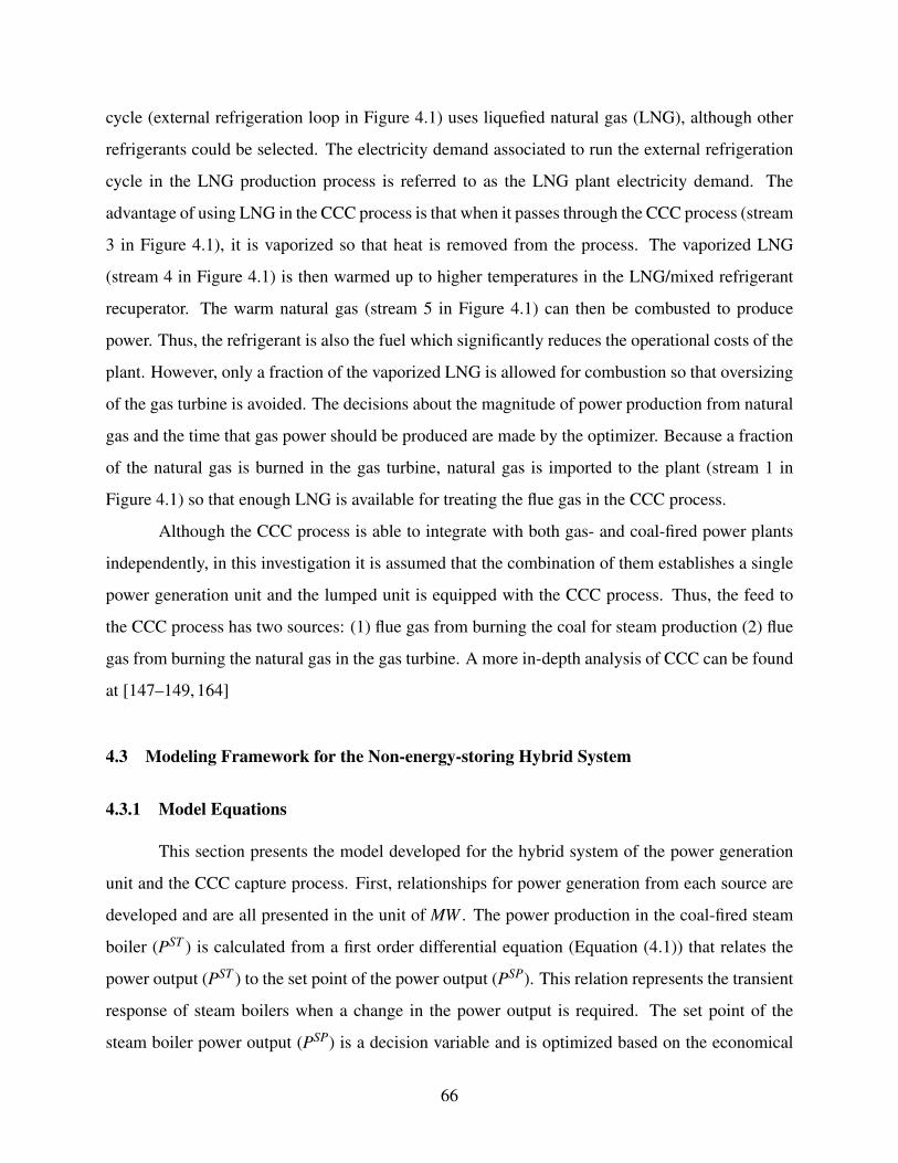
cycle (external refrigeration loop in Figure 4.1) uses liquefied natural gas (LNG), although other
refrigerants could be selected. The electricity demand associated to run the external refrigeration
cycle in the LNG production process is referred to as the LNG plant electricity demand. The
advantage of using LNG in the CCC process is that when it passes through the CCC process (stream
3 in Figure 4.1), it is vaporized so that heat is removed from the process. The vaporized LNG
(stream 4 in Figure 4.1) is then warmed up to higher temperatures in the LNG/mixed refrigerant
recuperator. The warm natural gas (stream 5 in Figure 4.1) can then be combusted to produce
power. Thus, the refrigerant is also the fuel which significantly reduces the operational costs of the
plant. However, only a fraction of the vaporized LNG is allowed for combustion so that oversizing
of the gas turbine is avoided. The decisions about the magnitude of power production from natural
gas and the time that gas power should be produced are made by the optimizer. Because a fraction
of the natural gas is burned in the gas turbine, natural gas is imported to the plant (stream 1 in
Figure 4.1) so that enough LNG is available for treating the flue gas in the CCC process.
Although the CCC process is able to integrate with both gas- and coal-fired power plants
independently, in this investigation it is assumed that the combination of them establishes a single
power generation unit and the lumped unit is equipped with the CCC process. Thus, the feed to
the CCC process has two sources: (1) flue gas from burning the coal for steam production (2) flue
gas from burning the natural gas in the gas turbine. A more in-depth analysis of CCC can be found
at [147–149, 164]
4.3 Modeling Framework for the Non-energy-storing Hybrid System
4.3.1 Model Equations
This section presents the model developed for the hybrid system of the power generation
unit and the CCC capture process. First, relationships for power generation from each source are
developed and are all presented in the unit of MW . The power production in the coal-fired steam
boiler (PST ) is calculated from a first order differential equation (Equation (4.1)) that relates the
power output (PST ) to the set point of the power output (PSP). This relation represents the transient
response of steam boilers when a change in the power output is required. The set point of the
steam boiler power output (PSP) is a decision variable and is optimized based on the economical
66

Figure 4.1: Schematic configuration of the integrated system of power generation unit and the CCC processwithout energy storage
evaluation of the hybrid system. The range of variation of PSP is considered between the nominal
capacity of the steam boiler and and 44% of this capacity. When integrating the CCC capture pro-
cess with existing power generation units, this range should be modified according to the capacity
of the steam turbine.
τST dPST
dt=−PST +KST PSP (4.1)
In this case, τST and KST are the time constant and gain, respectively, for power production
in the steam boiler. The time constant represents the time it takes to reach 63.2% of the total
change in steam boiler power output when there is a change in the set point. Gain is the ratio
of total change in the power output from the steam boiler and the magnitude of change in the set
point. An assumed value of 2 hours for the time constant represents the slow response of the steam
boilers to changes in set points in practice. A gain value of 1 is used in Equation (4.1) for the
steam boiler. It should be noted that reference to the power production in a steam boiler (PST ), in
67

this investigation, is in fact the result of producing power in a turbine that is driven by the steam
generated in the boiler. Steam is generated from the heat content of the flue gas produced from
coal combustion (simple cycle). Exiting flue gas from a gas turbine can also be introduced to the
boiler to produce more steam and achieve the efficiency of a combined cycle. Thus, total power
output from the steam turbine (PST ) in the combined cycle is the summation of equivalent power
from exchanging heat by the flue gas generated from coal and natural gas combustion (Equation
(4.2)).
PST = PCT +PNGCC (4.2)
PCT and PNGCC are the power generated from the coal and natural gas flue gases, respec-
tively. PNGCC is dependent on the rate of natural gas combusted in the gas turbine, NGConv, (or
equivalently on the gas power production, PGT ) and is defined in (4.4). Either PCT or PGT can
be selected as the second decision variable and the other variable (as well as PNGCC) is calculated
from solving Equations (4.2) and (4.4) simultaneously. Similarly, mass flow rates of combusted
coal (C) and natural gas (NGConv) can be selected as the second decision variable. In this investi-
gation, flow rate of the natural gas combusted in the gas turbine is selected as the second decision
variable. Power generated in the gas turbine, PGT , is then calculated from Equation (4.3):
PGT = NGConvεg∆Hg (4.3)
where εg, ∆Hg are the efficiency of power production in the gas turbine and enthalpy of combustion
of natural gas, respectively. The values assumed for these two parameters are 0.3275 and 53.89
MJ/kg, respectively [166]. It should be noted that all equations involving flow rates are presented
on a mass basis with units of kg/hr.
Power production from the steam generated from the natural gas combined cycle is ob-
tained from Equation (4.4). In deriving this equation, it is assumed that the heat transfer from the
flue gas to the boiler feedwater has an efficiency of 88% (εSB). It is also assumed that the steam tur-
bine is 41.6% efficient (ηST ). Ratio of the mass flow rates of the flue gas to natural gas combusted
in the gas turbine is presumed to be 42.56 kg/hr (Equation (4.5)). These assumptions are based on
the simulation studies for a NGCC power plant with a single reheat 16.5 MPa/566 ◦C/566 ◦C cycle
68

and an overall combined cycle efficiency of 50.2% [166]. Thus, the overall power production in
the steam turbine is the product of specific enthalpy change of the flue gas (∆HNGFG ), mass flow rate
of the flue gas produced from natural gas combustion (FGNG), efficiency of the heat exchange in
the boiler (εSB), and efficiency of the steam turbine (ηST ):
PNGCC = ∆HNGFG FGNG
εSB
ηST (4.4)
NGConv =FGNG
42.56(4.5)
As mentioned previously, solving Equations (4.2) and (4.4) simultaneously returns the
value of PCT . An equation similar to Equation (4.4) is then used to calculate the mass flow rate of
the flue gas from the combustion of coal (Equation (4.6)):
FGC =PCT
εSBηST ∆HCFG
(4.6)
In this case, FGC and ∆HCFG are the mass flow rate of the flue gas from coal combustion
and specific enthalpy change of the flue gas, respectively. It is also assumed that 10.93 kg/hr flue
gas is produced from the combustion of 1 kg/hr of coal (Equation (4.7)).
C =FGC
10.93(4.7)
All these assumptions are based on the simulated results from [166] for a subcritical pul-
verized coal power plant that uses a single reheat 16.5 MPa/566 ◦C/566 ◦C cycle and has an overall
plant efficiency of 36.8%. Table 4.1 summarizes most of the data used in this investigation.
Although flue gas produced in the gas turbine can be completely directed to the boiler, it is
assumed that only a fraction of it is used for excess steam generation in the boiler. This constraint
addresses the limitation of the steam boilers in utilization of the flue gas in a combined cycle. The
flow rate of the flue gas directed to the steam boiler is limited to a flow rate that can potentially
produce sufficient steam to generate power up to 20% of the assumed upper bound for the steam
turbine capacity and is calculated from Equations (4.8) and (4.9). It should be noted that the
69

Table 4.1: Summary of the input parameters
Parameter Value
Thermal efficiency of boiler, εSB 0.88
Efficiency of the steam turbine, ηST 0.416Specific enthalpy change of the flue gasfrom coal combustion, ∆HC
FG, (MJ/kg) 2.335
Efficiency of the gas turbine, εg 0.3275Enthalpy of combustion of natural gas
(HHV), ∆Hg (MJ/kg) 53.89
Specific enthalpy change of the flue gasfrom natural gas combustion, ∆HNG
FG (MJ/kg) 0.587
Overall efficiency of coal–fired power plant 36.8%
Overall efficiency of the NGCC power plant 50.2%Work of compression for natural gas
compressor (kWh/(kg inlet)) or (GJ/tonne CO2) 0.051 (0.1656)
Work of compression for mixed refrigerantcompressor (kWh/(kg inlet)) or (GJ/tonne CO2) 0.077 (0.1818)
Electricity demand of the CCC for treatmentof the flue gas (coal combustion)(GJ/(tonne CO2 captured))
0.389
Electricity demand of the CCC for treatmentof the flue gas (gas combustion)(GJ/(tonne CO2 captured))
0.428
LNG demand to process the coal flue gas(kg/(tonne CO2 captured))
856
LNG demand to process the gas flue gas(kg/(tonne CO2 captured))
685
numerator of Equation (4.8) is normalized with the capacity of the gas turbine to keep the units of
both sides on a mass basis.
NGConv,max =GPCC
maxGT cap NGConv (4.8)
FGNG,max = 42.56NGConv,max (4.9)
70

Table 4.2: Coal properties
Component Weight percentageCarbon 48.18
Hydrogen 3.310Oxygen 11.87Chlorine 0.01Sulfur 0.37
Nitrogen 0.7Ash 5.32
Moisture 30.24
NGConv,max represents the maximum flow rate of combusted natural gas, of which the cor-
responding produced flue gas ,FGNG,max, is directed to the steam boiler. The maximum permitted
power production in the combined cycle and the capacity of the gas turbine are represented by
GPCCmax, GT cap, respectively.
Next, electricity demand of the CCC and LNG production facilities and the LNG require-
ment to treat the flue gas are calculated. While the power production from natural gas in a com-
bined cycle is limited, all the flue gas produced in the gas turbine should be treated in the CCC
process. Thus, total electricity demand of the CCC process and the required LNG to treat the flue
gas resulting from the combustion of natural gas are based on NGConv and is calculated from the re-
arrangement of Equation (4.5). It is assumed that the treatment of hot flue gas from the gas turbine
and the cold flue gas from the steam boiler requires the same amount of electricity and LNG. Ac-
cording to [36], treatment of the flue gas produced from coal and natural gas combustion requires
0.389 and 0.428 GJ per tonne of captured CO2, respectively. Adopting the combustion reaction
mechanisms used by [151] for a subbituminous Wyoming Powder River Basin coal and natural gas
with the compositions given in Tables 4.2 and 4.3 [167] results in 851.23 and 545.47 kg/hr CO2
production from one MW power generation from coal and natural gas, respectively. With a 90%
capture rate, the electricity demands of the CCC process for treatment of the flue gases generated
from coal and natural gas combustion are 0.083 and 0.058 MW per one MW generated power from
each source, respectively. The overall electricity demand for the CCC facility is then calculated
from Equation (4.10):
DCCC = 0.083PCT +0.058PNGCC (4.10)
71

Table 4.3: Natural gas properties
Component Mole percentageMethane 83.4Ethane 15.8
Nitrogen 0.8
According to [36], required LNG to process the flue gases from coal and natural gas com-
bustion are 856 and 685 kg per tonne CO2 captured. Similar to the calculation of the CCC elec-
tricity demand, LNG demand for treatment of the flue gas from combustion of coal and natural gas
are 656.2 and 336.4 kg/hr per one MW generated power from each source, respectively. Thus, the
overall LNG demand is calculated from Equation (4.11):
LNGR = 656.2PCT +336.4PNGCC (4.11)
The work of compression of the natural gas (DNG,Comp) and mixed refrigerant (DMR,Comp)
compressors are 0.051 and 0.077 kW per kg/hr of the inlet streams, respectively [36]. After unit
conversion, these lead to the following equations:
DNG,Comp = 5.1×10⁻⁴NGCCC (4.12)
DMR,Comp = 7.7×10⁻⁵MR (4.13)
In this case, NGCCC and MR are the mass flow rates of natural gas coming from the CCC
process and mixed refrigerant, respectively. Total electricity demand of the LNG production facil-
ity, DLNG, is the summation of DNG,Comp and DMR,Comp (Equation (4.14)).
DLNG = DNG,Comp +DMR,Comp (4.14)
Total electricity demand from the CCC and LNG production facilities, Dplant , is then cal-
culated by adding up the individual components (Equation (4.15)):
Dplant = DCCC +DLNG (4.15)
72
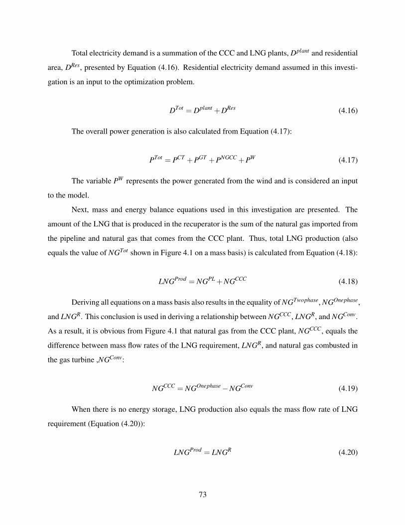
Total electricity demand is a summation of the CCC and LNG plants, Dplant and residential
area, DRes, presented by Equation (4.16). Residential electricity demand assumed in this investi-
gation is an input to the optimization problem.
DTot = Dplant +DRes (4.16)
The overall power generation is also calculated from Equation (4.17):
PTot = PCT +PGT +PNGCC +PW (4.17)
The variable PW represents the power generated from the wind and is considered an input
to the model.
Next, mass and energy balance equations used in this investigation are presented. The
amount of the LNG that is produced in the recuperator is the sum of the natural gas imported from
the pipeline and natural gas that comes from the CCC plant. Thus, total LNG production (also
equals the value of NGTot shown in Figure 4.1 on a mass basis) is calculated from Equation (4.18):
LNGProd = NGPL +NGCCC (4.18)
Deriving all equations on a mass basis also results in the equality of NGTwophase, NGOnephase,
and LNGR. This conclusion is used in deriving a relationship between NGCCC, LNGR, and NGConv.
As a result, it is obvious from Figure 4.1 that natural gas from the CCC plant, NGCCC, equals the
difference between mass flow rates of the LNG requirement, LNGR, and natural gas combusted in
the gas turbine ,NGConv:
NGCCC = NGOnephase−NGConv (4.19)
When there is no energy storage, LNG production also equals the mass flow rate of LNG
requirement (Equation (4.20)):
LNGProd = LNGR (4.20)
73

While combustion of the natural gas in the gas turbine is approximately instantaneous, an
equation similar to Equation (4.1) is considered for the natural gas imported to the plant (Equation
(4.21)). This equation represents the dynamic response of the system to changes in set point of
imported natural gas.
τNG dNGPL
dt=−NGPL +KNGNGPL,SP (4.21)
where NGPL,SP is the set point of the natural gas imported from the pipeline and is a deci-
sion variable. Time constant and gain of the first order model used in this equation are represented
by τNG and KNG, respectively. A time constant of 5 minutes and a gain value of 1 are assumed for
the import of natural gas.
An energy balance over the recuperator defines the relationship between the natural gas
imported (NGPL) and recirculated in the system (NGCCC). It also defines the trend of variation of
mass flow rate for the mixed refrigerant (MR). Total energy gain from the cold streams entering
the recuperator is obtained from Equation (4.22):
Qg = NGTwophase∆H1 +MR∆H2 (4.22)
where ∆H1 is the enthalpy difference of the two phase gas stream exiting the CCC plant
and warm natural gas after the recuperator and is equal to 299 kJ/kg. ∆H2 is also the enthalpy
difference of the cold mixed refrigerant entering the recuperator and is equal to 620 kJ/kg.
Total energy loss from the hot streams entering the recuperator is also obtained from Equa-
tion (4.23):
QL = NGTot∆H3 +MR∆H4 (4.23)
where ∆H3 is the enthalpy difference between the warm natural gas that is liquefied and
the LNG produced in the plant and is equal to -582 kJ/kg. ∆H4 is also the enthalpy difference of
the hot mixed refrigerant entering the recuperator and is equal to -9 kJ/kg.
The values assumed for ∆H1, ∆H2, ∆H3, and ∆H4 are based on the results obtained at [147]
with the assumption that temperature and pressure of the entering and exiting streams to and from
the recuperator are constant. Results presented in [168, 169] propose a design for a plate heat
74

exchanger that the temperature and pressure remain constant despite the fluctuations in inlet and
outlet conditions of the heat exchanger. These fluctuations occur because of the process transients
introduced by energy storage and specifically by large swings in LNG production rates in response
to the variations in electricity demand and wind power. The proposed design is able to minimize
the transient impacts of energy storage and LNG production on the operating conditions of the heat
exchanger. Thus, the recuperator considered in this study has a steady–state performance and is
very responsive to fluctuations in the inlet and outlet conditions of the recuperator.
The summation of Qg and QL should be zero, assuming no heat loss to the environment
(Equation (4.24)).
Qg +QL = 0 (4.24)
Finally, the objective function is defined as follows:
Pro f it = (DRes−DPlant)PE − (NGPL)PN−PCC (4.25)
where PE , PN , and PC represent energy price ($/MWh), natural gas price ($/kg), and coal
price ($/kg), respectively. An hourly energy price is also assumed in this study. This investigation
focuses on operating costs, though levelized capital costs could be introduced to the cost functions
if investment decisions are to be included.
4.3.2 Controlled variable
The overall power generation from the coal, gas, and wind should always match the sum
of the electricity demands for the residential users and the CCC and LNG production facilities, as
shown with Equation (4.26)
PTot = DTot (4.26)
To achieve this goal, excess energy production is defined as shown in Equation (4.27) and it
is considered as a controlled variable with high and low set point values of zero. This also permits
75

the assignment of a higher penalty for underproduction of power. Selection of a value of zero for
the high and low set points of excess energy production highlights that neither overproduction nor
underproduction of power is an optimal solution in practice.
PEx = PTot−DTot (4.27)
4.3.3 Constraints
Power produced in the gas turbine should always be less than its capacity.
PGT ≤ GT cap (4.28)
Steady state simulations have shown that the combined electricity demand of the LNG
and CCC plants is 15-20% of the power generated in the power plant [147]. A value of 20% is
adopted for Dplant,max in the results presented in this Chapter [170] while a lower value of 15% is
considered for the results presented in Chapters 5 and 6 [36]. However, the optimization results
shown in Section 4.5 demonstrate that Dplant is always less than 15% of PSP,Max.
Dplant ≤ Dplant,maxPSP,Max (4.29)
After formulating the system, it is necessary to set up an optimization framework to in-
crease the effectiveness of the hybrid system. The optimization framework used in this system
benefits from an objective function in the form of an `1-norm (2.5). In this equation, a desired ob-
jective function for the problem (Equation (4.25)) is added to the expression presented by Equation
(2.5a) and forms the overall objective function. The mathematical equations presented by Equa-
tion (2.5) are used to tune the model to obtain satisfactory results; i.e., in each simulation, variables
cy,cu,c∆u are adjusted such that smooth results are observed in the trend of the decision variables.
Thus, these variables are the tuning parameters for the model. High penalization factors are also
assigned for the deviation of the controlled variable from the desired set point. The penalization
factors are wh and wl to penalize over and under production of power, respectively.
The set of equations discussed is implemented in the APMonitor Modeling Language [29]
and solved either with an interior point solver (IPOPT) [71] or an active set solver (APOPT [140,
76

141]. More information about how to implement an optimization in the APMonitor Modeling
Language can be found in [35].
4.4 Model Implementation
In this section, the model developed for the hybrid system of power generation and the
non-storing version of the CCC process is implemented with a set of assumptions and input data.
In this case, it is assumed that power production in the coal–fired generation unit is based on a
simple cycle; i.e. FGNG,max is zero which results in PNGCC be equal to zero).
4.4.1 Model Inputs
In this study, the power output of ten wind power stations, each comprising multiple wind-
mills, in southern California, USA is considered along with coal and gas power generation units.
The maximum actual power output from the wind stations is 300 MW while steam boiler has a
capacity (PSP,Max) of 1200 MW . The steam boiler considered in this investigation is also able to
follow the electricity load at a maximum change rate of 7% per minute [171]. A capacity of 240
MW is considered for the gas turbine. A more accurate analysis of the size of the gas turbine is
made by considering capital cost of the equipment and is outside the scope of this dissertation.
The electricity demand profile adopted for this section is related to the forecasted data for a
zone in southern California, USA. Electricity demand data is taken from [172]; this is the predicted
data for 2022 with a maximum of 1200 MW . The assumed data for these variables are typical for
most residential areas. The wind power [173] and electricity power prices [174] are represented by
2006 and 2009 data, respectively. Two time periods are selected to compare the effect of seasonal
changes on electricity demand and weather condition. The first time period is between July 18th
and July 20th (summer case), when the peak electricity demand of the year is predicted to occur.
The second time period is between January 25th and January 27th (winter case), when wind power
had the highest standard deviation among all possible three consecutive day time horizons in 2006.
Trends of variation of electricity demand data and energy price are presented in Figures 4.2 and
4.3 for the summer and winter, respectively. Trend of wind power for each scenario is shown along
with the optimization results shown in Section 4.5.
77

Figure 4.2: 2022 forecasted electricity demand data for a zone in southern California, USA (Summer case)[172].
The simulation time horizon considered in this investigation is 72 hours with one hour time
discretization.
4.5 Optimization Results
4.5.1 Comparison Between Summer and Winter Results
The main results of the optimization of the integrated system without energy storage for
both summer and winter cases are presented in this section. The summer case result, displayed in
Figure 4.4, shows that the total power produced in the system is always greater than or equal to the
total electricity demand. The total excess power over the time horizon is approximately zero in this
scenario. Coal power is the main source of the electricity generation, while gas power is produced
78

Figure 4.3: 2022 forecasted electricity demand data for a zone in southern California, USA (Winter case)[172].
during peak hours to meet the total electricity demand. Whenever wind is available, it is used first
to meet the demand. Coal power is mainly dispatched after the wind while gas power is mostly
produced in periods with high electricity demand. Optimization shows a maximum change rate of
0.3% per min for the load in the steam boiler that is less than the maximum anticipated change rate
of 7% per minute. Figure 4.4 shows that the combined LNG and CCC electricity demands satisfy
the constraint described in Section 4.3.3.
For the winter case (shown in Figure 4.5), the electricity demand decreases significantly and
wind power is more readily available than in the summer case. In fact, there are times (such as the
period between hours 26 and 29) when wind power can fully meet the total electricity requirement
of the residential area and the CCC and LNG plants. Therefore, power production from coal and
gas are not needed and are reduced to zero. Wind power also has a high rate of fluctuation in
79

Figure 4.4: Power vs. electricity demand profile (summer case)
the winter. Thus, when wind power is not sufficient to meet the total electricity demand or when
it is fluctuating frequently, both gas and coal power are used to compensate for the lack of wind
power. Gas power is used as much as possible during peak hours and when wind power is not
sufficient. After reaching the maximum allowable limit for gas power, coal power is used to meet
the electricity demand. The total excess power over the time horizon is less than 0.6% in this
scenario. The maximum rate of load change in the steam boiler (0.2% per min) is also less than the
maximum anticipated change rate of 7% per minute. Similar to the summer case, the combined
electricity demand for the LNG and CCC plants is less than the assumed upper bound (240 MW ).
80

Figure 4.5: Power vs. electricity demand profile (winter case)
The range of operation of the steam boiler used in this study is considered to vary from zero
to full capacity. While it is important to show the concept of more wind utilization by assuming a
lower limit of zero for the steam boiler, the zero limit is not practical. The lower limit of the steam
boiler is selected to be zero to add enough flexibility to the hybrid system so as to not produce
excess power. A longer time frame and economical evaluations are needed to find an appropriate
boiler capacity. In that case, the simplifying assumption for the lower limit of power output from
the steam boiler can be easily modified. Adding the energy storage capability of the CCC process
is another viable option to make the rate of change of the boiler smoother [36].
81
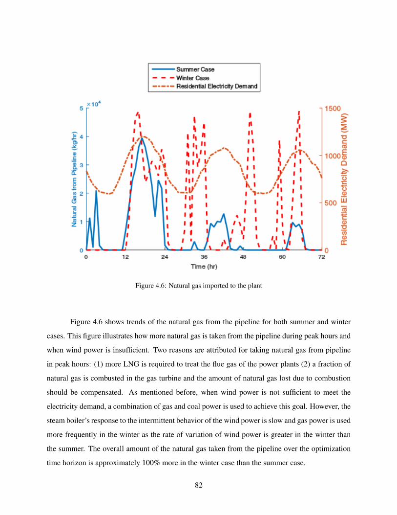
Figure 4.6: Natural gas imported to the plant
Figure 4.6 shows trends of the natural gas from the pipeline for both summer and winter
cases. This figure illustrates how more natural gas is taken from the pipeline during peak hours and
when wind power is insufficient. Two reasons are attributed for taking natural gas from pipeline
in peak hours: (1) more LNG is required to treat the flue gas of the power plants (2) a fraction of
natural gas is combusted in the gas turbine and the amount of natural gas lost due to combustion
should be compensated. As mentioned before, when wind power is not sufficient to meet the
electricity demand, a combination of gas and coal power is used to achieve this goal. However, the
steam boiler’s response to the intermittent behavior of the wind power is slow and gas power is used
more frequently in the winter as the rate of variation of wind power is greater in the winter than
the summer. The overall amount of the natural gas taken from the pipeline over the optimization
time horizon is approximately 100% more in the winter case than the summer case.
82

The same trend is observed for the LNG production rate (Figure 4.7). During off peak
hours, less LNG is required and it is produced from the recirculating natural gas inside the plant
(stream 7 in Figure 4.1). Since more LNG is required during peak hours, the necessary LNG is
supplied from both pipeline and recirculating natural gas. The overall amount of LNG produced
inside the plant for the winter case is 80% less than the summer case. This difference is attributed
to the higher penetration of wind power into the power production unit in the winter. In addition,
gas power is produced more than the coal power in the winter case. As CO2 emissions from
the gas combustion are less than from coal combustion, smaller amounts of LNG are required to
run the CCC process during the winter. Thus, when more wind power is adopted into the power
generation units, the LNG production rate decreases. The same behavior is observed for the sum
of the electricity demands for the LNG and CCC plants.
The average operational profit obtained from the integrated system, assuming a constant
natural gas price, is approximately $21k/hr for the summer case. The average operational profit
for the winter case is approximately $13k/hr. The higher profit obtained for the summer case is
expected as larger variation in the electricity price creates more benefit from the hybrid system.
4.5.2 Sensitivity Analysis for Wind Power Adoption
Finally, a sensitivity analysis is implemented to compare the effect of different rates of wind
power adoption on the utilization of coal and gas power. For the cases outlined in this section, the
winter data and a wind adoption factor (α) are used to define the fraction of the available wind
power adopted in power generation. When α = 1, all of the available wind power is adopted to
meet the electricity demand, while α = 0.5 means that only half of the available wind power is
used. As shown in Figure 4.8, adopting more wind power causes less coal power production.
However, gas power has higher influence at higher wind power adoption rates; this is due to its fast
response to the intermittent behavior of the wind power. Using more gas power is advantageous
as coal power produces more CO2 and using more wind and gas power results in lower electricity
demands for the LNG and CCC plants. Conversely, lower adoption of the wind power requires
more power to be produced from coal to meet the total electricity demand.
The impact of the adoption factor on the profitability of the hybrid system is shown in
Figure 4.9. The revenue of sale of electricity to residential consumer is constant at all values of
83

Figure 4.7: LNG production in the system
α . Coal cost and the electricity cost to run the LNG and CCC plants decrease by adopting more
wind power into the power generation units. However, gas cost increases by increasing the wind
power adoption factor. This conclusion is expected because gas power, as opposed to coal power,
is used more to meet the total electricity demand when more wind power is adopted. It is observed
from Figure 4.9 that at α = 0.66 the integrated profit over the simulation time is at a maximum.
This means that at this value, a combination of the three power sources lead to the maximum
profit obtainable from this system for the winter case. Thus, further adoption of the wind power
does not increase profitability in the assumed hybrid system. The average profit obtained from
the hybrid system at a wind adoption factor of α = 0.66 is $14.5k/hr. The natural gas price used
to obtain results in Figure 4.9 is an average value of 5.74 $/Mcf. However, the same trend in the
profitability is obtained with a natural gas price ranging from 3.54 to 18.25 $/Mcf. This price range
84

Figure 4.8: Impact of wind power adoption factor on power production from gas and coal (winter data)
is sufficiently wide to capture the possible growth in the natural gas price in 2022 [175,176] and is
sufficient for the purpose of this study. Change in the coal price from 12.65 $/ton to 17 $/ton (the
projected price for the Powder River Basin coal in 2022) also leads to the same conclusions.
4.6 Conclusion
The impact of the CCC process (a post-combustion CO2 removal process) on fossil-fueled
power plants is considered in this chapter. The CCC process is considered as a response to the
tightening restrictions on CO2 emission from fossil-fueled power plants (such as the new regula-
tions recently unveiled by the EPA in the Clean Power Plan). The fast response of the CCC process
to electricity demand helps utilize more renewable energy sources on the grid, which emits less
CO2. The effects of seasonal variations in electricity demand and wind availability are investigated
by considering the summer and winter cases. The proposed hybrid system is able to meet the total
85

Figure 4.9: Operating costs and electricity demand revenue vs wind power adoption factor (α) (winter data)
electricity demand. All of the available wind power is utilized in this study to meet the electricity
demand. The operating profit obtained from the proposed system for the summer case is $21k/hr,
while the winter case profit is approximately $13k/hr. The larger availability of wind power in
the winter leads to 100% more intake of natural gas to the plant than in the summer case. LNG
production over the optimization time horizon decreases by 80% for the winter case.
A sensitivity analysis examines the change in operating strategy of the proposed system
with respect to the wind power adoption factor (α ). At higher values of α , coal power utiliza-
tion decreases while gas power utilization increases. At α = 0.66, the profit obtained to run the
integrated system in the winter is at a maximum.
The hybrid system of a load–following power generation unit and the CCC process with
the associated energy storage facilities is addressed in Chapter 5. Furthermore, the impact of the
CCC process on a baseline power plant is the focus of Chapter 6.
86

CHAPTER 5. INVESTIGATING THE IMPACT OF ENERGY-STORING CRYOGENICCARBON CAPTURE ON POWER PLANT PERFORMANCE
5.1 Introduction
As mentioned in Chapter 4, the CCC process requires two refrigeration loops that consume
most of the energy in running the compressors. However, refrigerant can be generated during non-
peak hours and stored in insulated vessels that save the refrigerant for peak hour usage, thereby
replacing the compressor energy with the stored refrigerant. This causes the refrigerant production
rate to decrease during peak hours, which decreases the energy demand required by the CCC for
as long as the stored refrigerant is available. Therefore, more power is available during peak
hours relative to the baseline coal boiler rated capacity. Generating the refrigerant during non-peak
hours, when electricity is cheaper, also results in higher profits. In this investigation, storage of
only one of the refrigerants is considered as it provides more energy during the recovery mode.
The refrigerant considered for this purpose is LNG, although others could be selected.
In addition, the LNG generation and storage cycle primarily involves compressors and
heat exchangers; therefore, the storage/recovery or load changing response time is fast (seconds)
compared to those of the steam boilers (hours). The faster energy storage response time is well
matched to intermittent sources like wind turbines. Therefore, this energy storage system enables
the steam boiler to follow rapidly changing loads. Storage capacity of LNG vessels also allows
scaling from the proposed energy storage to large-scale systems.
The hybrid system of power generation units and energy-storing version of the CCC process
is shown in Figure 5.1. To better represent the storage and recovery modes of operation, a stream
(stream 6 in Figure 5.1) bypasses the tank. The storage tank allows natural gas to be imported from
the pipeline and converted to LNG during periods with low electricity prices. The fraction of the
produced LNG required to run the CCC process during off peak hours directly flows toward the
process through the bypass stream. The excess LNG flows to the tank inlet (stream 5 in Figure
87
5.1). During peak hours or periods with expensive electricity prices, LNG is supplied from two
sources: (1) the storage tank (2) the liquefaction of the recirculating natural gas. As for the case
study without energy storage, the LNG directed to the CCC process (stream 8 in Figure 5.1) is
vaporized so that heat is removed from the process. The natural gas coming from CCC (stream 9
in Figure 5.1) has sufficient cooling potential to be used to liquefy a fraction of the recirculating
natural gas (stream 13 in Figure 5.1). Thus, by passing the cold natural gas coming from the CCC
(stream 9 in Figure 5.1) through the LNG/mixed refrigerant (MR) recuperator, heat is recovered
from the warm recirculating natural gas (stream 13 in Figure 5.1). Therefore, a fraction of the
required LNG for running the CCC process is supplied from the recirculating natural gas. The rest
of the required LNG is supplied from the tank (stream 7 in Figure 5.1). Thus, LNG production
is ramped down during peak hours by using an LNG storage tank; i.e. the parasitic loss of the
mixed refrigerant compressor decreases in peak hours or when electricity is expensive. However,
it should be emphasized that at any given time, either the storage or recovery mode is always in
operation. The combination of the LNG storage tank, LNG/MR recuperator, mixed refrigerant
compressor, and natural gas compressors used in LNG production is referred to as the LNG plant.
Another option to decrease energy consumption in the LNG plant is to export a fraction of
the recirculating natural gas to the pipeline (stream 1 in Figure 5.1) and avoid processing it in the
LNG/MR recuperator. However, the pressure of the natural gas before the natural gas compressor
is approximately 11 bar and the pressure of the pipeline natural gas is approximately 55 bar; thus,
the pressure must be increased to pipeline pressure if natural gas is to be exported. A pressure
increase is implemented in two stages in this study: (1) in the natural gas compressor (from 11 to
37 bar) and (2) in the pipeline compressor (from 37 to 55 bar). The pressure increase in the natural
gas compressor should always occur, even if natural gas is not exported to the pipeline. However,
the pressure increase in the pipeline compressor does not significantly increase the parasitic loss of
the plant (approximately 3.2 MW). The exported natural gas also offers a lower CO2 concentration
and is more pure than the imported natural gas because of the purification that occurs through
the refrigeration cycle. The natural gas export is a cost saving measure for the integrated system
as it recovers part of the operating costs for unused natural gas. However, the price value of the
more pure natural gas is the same as the natural gas from the pipeline in this investigation and
is not awarded extra credit for the purification. This is mainly because of the unwillingness of
88

Figure 5.1: Schematic configuration of the integrated system of power generation unit and the CCC processwith energy storage
the utility contractors to buy back natural gas at a higher price. In other words, if natural gas is
to be simultaneously purchased or sold to utility contractors, the sale and purchase price will be
equal. This study assumes constant natural gas price. Decisions about whether natural gas should
be exported or imported at each time step are based on the economic evaluation of the objective
function.
The focus of this chapter is on the optimization of the hybrid system of power generation
units and the CCC process with consideration of the energy storage of the capture system. The
coal–fired power plant considered in this chapter is capable to follow the electricity demand load
with a maximum change rate of 7% per minute. The remainder of this chapter is divided into four
sections; in the first section, an example case study is discussed to demonstrate the concept of peak-
shaving of the electricity demand by using an energy storage system. Then, some of the equations
developed in chapter 4 are modified to account for the energy storage and export of natural gas to
89

pipeline. Next, the inputs for this hybrid system are presented. Finally, simulation results for the
integrated system are discussed.
5.2 Example Case Study for Energy Storage Concept
In this section, an example case study is developed to demonstrate the energy storage con-
cept. The main power generation unit output is assumed to be constant in this case. Excess energy
is stored during off-peak hours or when more energy is available than the required electricity de-
mand. The stored energy is used during peak hours to meet the higher electricity demand. The
objective is to minimize the power production unit output. This goal is obtained by efficiently
using the energy storage system to meet the cyclical demand cycle that is typical for a grid-scale
power distribution system. The assumed demand profile has a periodic form that is typical for both
industrial and residential areas. As energy storage and energy recovery are not coincident, slack
variables are used in this example case to help the optimizer switch between energy storage and
energy recovery. The time horizon considered for this simplified case is 24 hours with 20 minute
time discretization.
The equations used to model this simplified case are given below. These equations represent
a simple power dispatching system and demonstrate the concept of peak-shaving of the electricity
demand by using an energy storage system.
min P (5.1a)
s.t.δ Iδ t
= S · ε−R (5.1b)
S = P−D+S2 (5.1c)
R = D−P+S1 (5.1d)
P−D = S1−S2 (5.1e)
S1,S2 ≥ 0 (5.1f)
S1×S2 ≤ 0 (5.1g)
90

P+R−S≥ D (5.1h)
I ≥ 0 (5.1i)
where P,D,S,R and I represent power production, electricity demand, stored energy, recovered
energy, and inventory of stored energy, respectively. S1 and S2 are slack variables to help switch
between energy storage and energy recovery and are constrained to be positive. The efficiency
loss during storage of energy is represented by ε . Equation (5.1a) defines the objective function.
Equation (5.1b) represents the energy balance for the energy storage system. Equations (5.1c) and
(5.1d) represent the magnitude of the stored and recovered energy, and Equation (5.1e) defines
the magnitudes of S1 and S2. Equations (5.1f) and (5.1g) ensure that storage and recovery modes
do not operate simultaneously (either S1 or S2 or both should be zero during the time horizon).
Equation (5.1h) guarantees that power supply from power production and energy recovery, with
consideration of the storage of energy during off peak hours, is always greater than the electricity
demand. Equation (5.1i) ensures that energy inventory is always greater than or equal to zero.
According to the optimization framework proposed previously, Equation (5.1c) to (5.1e) serve as
the equality constraints (Equation (2.5c)) while and Equation (5.1f) to (5.1i) serve as the inequality
constraints (Equation (2.5d)).
When S2 is zero, S1 is equal to P−D, according to Equation (5.1e). Consequently, S
equals excess energy (P−D) based on Equation (5.1c) and R equals zero in agreement with Equa-
tion (5.1d). Thus, this case represents the storage mode, and the inventory of the storage system
increases according to Equation (5.1b). When S1 is zero, S2 becomes D−P from Equation (5.1e).
Consequently, R equals D−P from Equation (5.1d) and S equals zero. Thus, this case represents
the recovery mode, and the inventory of the storage system decreases according to Equation (5.1b).
Results of the simplified case are presented in Figure 5.2. As shown in the figure, when
power generation is more than the required electricity demand, energy is stored and the energy
inventory of the storage system increases. When electricity demand is greater than the power
production, energy is recovered from storage and energy inventory in the storage system decreases.
Slack variables show consistent trends with these findings. This example case demonstrates the
energy storage optimization concept used in the more detailed case of power production with CCC.
91

Figure 5.2: Results for the simplified case of energy storage
5.3 Modeling Framework for the Energy-Storing Hybrid System
5.3.1 Governing Equations
This section considers the modification of some of the equations developed in Chapter 4 to
account for the energy storage and export of natural gas to pipeline. Except for the equations and
figures that are modified in this chapter, similar relationships used in Chapter 4 are used for the
hybrid system with energy storage.
In the system considered in this chapter, the flow rate of natural gas exported to the pipeline
is deducted from the total recirculating natural gas (NGTot). As all relations are expressed on a mass
basis, NGTot also equals LNGProd . Thus, total LNG production should also be modified (Equation
(5.2)). The energy balance over the recuperator is also modified accordingly.
92

LNGProd = NGPL +NGCCC−NGEXPT (5.2)
In this case, NGEXPT represents the natural gas exported to the pipeline (kg/hr) and is a
decision variable. Produced LNG also equals the summation of the LNG to the tank and the LNG
bypassing the tank Equation (5.3):
LNGProd = LNGTo Tank +LNGBY P (5.3)
In Equation (5.3), LNGTo Tank and LNGBY P represent the LNG directed to the tank and the
amount that bypasses it. LNGTo Tank is also a decision variable in the hybrid system with energy
storage. LNG from the tank is calculated from a mass balance at the tank outlet Equation (5.4):
LNGFrom Tank = LNGR−LNGBY P (5.4)
A dynamic mass balance equation is also developed in Equation (5.5) for defining the
inventory of tank, LNGTank:
d(LNGTank)
dt= LNGTo Tank−LNGFrom Tank (5.5)
The work of compression of pipeline compressor (DNG,Pipe) is 0.01 kW per kg/hr of the
inlet stream [36] and is based on the results obtained previously [147, 164]. After unit conversion,
this leads to the following equation:
DNG,Pipe = 1×10⁻⁵NGEXPT (5.6)
The total electricity demand from the CCC and LNG production facilities, Dplant , is then
calculated from Equation (5.7):
Dplant = DCCC +DNG,Comp +DMR,Comp +DNG,Pipe (5.7)
The profit function used in this investigation is also modified to account for the export of
natural gas Equation (5.8).
93

Pro f it = (DRes−DPlant)PE − (NGPL−NGEXPT )PN−PCC (5.8)
An hourly energy price is also assumed in this analysis. As mentioned before, the credit
given to export of the natural gas is considered to be the same as the purchasing price of the
imported natural gas. The electricity demand profile is an input to the model and is not a decision
variable. Revenue obtained from selling the electricity (first term in the right hand side of Equation
5.8) is constant in all scenarios considered in Section 5.5. Thus, the optimizer actually tries to
optimize the profit function from the remaining expressions in Equation 5.8. Using the electricity
demand in the profit function, however, would provide a comparison basis for the profitability of
the hybrid system.
A time horizon of eight days with one hour time increments is considered for profit max-
imization. By removing the boundary conditions, the performance of the three middle days rep-
resents an infinite time horizon. Because of the complexity of the model and the large number of
variables and equations to be solved, initialization strategies developed in Chapter 2 are applied to
decrease the computational time of the simulations.
5.3.2 Constraints
As mentioned in Section 5.1, either energy storage or an energy recovery mode is in op-
eration at each time step. The selection of operating mode depends on the economic evaluation
of each time step. The constraint developed in Equation (5.9) helps the optimization algorithm
choose between the operational strategy at each time step:
LNGTo TankLNGFrom Tank = 0 (5.9)
While this constraint assumes that either LNGTo Tank or LNGFrom Tank is zero at each time
step, LNGBY P always has non-zero values. This is because of the continuous demand of LNG to
the CCC plant for the treatment of CO2 produced from the power plant. It is also unlikely that
import and export of natural gas occur simultaneously in practice. Thus, a similar relationship is
assumed between them (Equation (5.10)):
94

NGPLNGEXPT = 0 (5.10)
5.4 Model Inputs
In this investigation, a residential electricity demand profile is used as the actual hourly
integrated data for San Diego, USA, for the period between September 13, 2014 and September
20, 2014. These data give the peak electricity demand of the year in the area [177]. Because
this study represents the integration of the CCC process with only one power generation unit,
the electricity demand data is scaled to have a maximum residential demand of 2000 MW. The
assumed electricity demand profile is typical for many residential areas and is shown in Figure
5.3. The average price of electricity for the same period in 2014 for California is also shown in
Figure 5.3 [178]. It is seen from Figure 5.3 that periods with high electricity demand also have
more expensive power price. Wind data shown in Figure 5.4 are based on the actual wind power
data for the same period of time in 2014 for southern California (SP-15 trading hub) [177]. This
study assumes that wind power only contributes up to 10% of the integrated residential demand
over the time horizon. Thus, total actual hourly wind power data from the SP-15 trading hub
is uniformly scaled down such that integrated wind power over the time horizon is approximately
10% of the integrated residential demand used in this investigation. It should be mentioned that the
assumed residential electricity demand and wind power curves are for one of the possible worst-
case scenarios (summer days) when the electricity demand reaches the maximum of the year in the
assumed zone in California in 2014. The trend of the power price in the period of time considered
in this investigation shows less spikes than the rest of the year [178]. More severe fluctuations are
expected to improve the economic justification for energy storage with the CCC. A typical period
was therefore selected over an extended time frame without inflating the benefits.
As for the case without energy storage, excess natural gas produced from the hybrid sys-
tem is combusted in a gas turbine for power production. The hot gas outlet from this turbine is
combined with the coal gases in the boiler convection pass, which gives the turbine the efficiency
of a combined-cycle system. Thus, a fraction of the flue gas from gas turbine (stream 18 in Figure
5.1) is directed to the steam boiler to produce steam for power generation and the rest of it (stream
26 in Figure 5.1) is directed to the CCC plant. Despite the fact that the flue gases produced from
95

Figure 5.3: Actual electricity demand for San Diego, USA, and average power price for California for theperiod between September 13, 2014 and September 20, 2014 [177, 178].
coal and gas combustion have different compositions, it is assumed that the flue gas exhausts from
both streams are treated with the same CCC process for simplicity (Figure 5.1). One approach to
operating with only one boiler for both flue gas exhausts is to consider a recirculation cycle after
the gas turbine, in which part of the natural gas flue gas is recirculated and introduced back into
the compressor inlet. As a result, the CO2 concentration of the natural gas flue gas directed to the
boiler can be increased to the coal flue gas CO2 level [179–181]. The recirculation concept is the
subject of future work and is not included in this contribution.
In addition, it is presumed that the set point of power production in the steam turbine (PSP)
can vary from 800 to 1800 MW . The capacity of the gas turbine is also assumed to be 50% of the
maximum residential electricity demand (2000 MW ) considered in this investigation (see Table
5.1). While the presumed turbine capacity is large and is not a typical capacity size in practice, it
96

Figure 5.4: Actual wind power data for the period between September 13, 2014 and September 20, 2014[177].
should be noted that the assumed electricity demand profile has a large range of variation (838 to
2000 MW ). Because the gas and steam turbines considered in this work are the main energy sources
during peak hours and the steam turbine is anticipated a baseline unit, it is not possible to meet the
peak of the residential electricity demand without a large gas turbine. With current technologies,
such a large fluctuation in electricity demand is met through several peaking generation units. Thus
the need for oversized gas or oil turbines is eliminated. With a single power generation unit it is
not possible to meet the large gap between maximum and minimum electricity demand. The need
to optimize load following capacity highlights the importance of simulating a power grid in which
the fossil–fueled power generation units are equipped with the CCC process. In this case, peak
97

Table 5.1: Additional input parameters for the case with energy storage
Parameter Value
GPCCmax (MW )
360 (20% of the upper bound for thesteam turbine power output)
Maximum residential electricity demand (MW ) 2000Gas turbine capacity (GT cap) (MW ) 1000
electricity demand is met through a combination of power sources. In addition, the energy storage
portion of CCC can effectively become the grid spinning reserve by adjusting its parasitic load in
time to accommodate the dispatch schedule of the grid. This large–scale energy storage capacity
has the potential for significant economic and operational benefit. Study of a large scale power grid
system when fossil–fueled power generation units are equipped with the CCC process is the focus
of future work. For the purpose of a single generation unit, it is assumed that a large capacity for
the gas turbine is a valid assumption. The pressumed overall efficiencies of the coal and gas-fired
power plants are also 36.8% and 50.2%, respectively, based on higher heating values (HHV) [166].
The coal composition used in this work is that of the subbituminous Wyoming Powder
River Basin coal as given in Table 4.2. Delivered coal price for Wyoming Powder River Basin is
assumed to be $12.65/ton as of March 2014 [182]. Composition of the imported natural gas is also
taken from Table 4.3. Natural gas price is the US national average price of 2014 for the electric
power sector ($5.19 per thousand cubic feet) [183]. Long-term contracts can be secured to reduce
the variability of fuel costs from sources such as natural gas.
The set of equations discussed in this chapter along with those described in Chapter 4 is
implemented in the APMonitor Modeling Language [29] and solved either with an interior point
solver (IPOPT) or an active set solver (APOPT).
5.5 Results and Discussion
This section presents the results of the optimization of the integrated system with energy
storage. The results are for a case study with an LNG tank capacity of 8 million kg. This tank
capacity is selected based on the performance of the hybrid system because the overall trend of
variables does not change with different tank sizes. As mentioned previously, all variables are
98

presented in mass units to remain independent of the pressure and temperature conditions of the
LNG tank. For typical LNG at the tank temperature and pressure of -94 °C and 37 bar (LNG
density is 290.6 kg/m3), the standard capacity for the 8 million kg LNG inventory is 28000 m3,
which is small compared to LNG tanks in commercial use and represents a very small incremental
expense as a fraction of the overall CCC process and power plant.
Electricity demand and power production curves (Figure 5.5) show that a dynamic combi-
nation of power sources meets the power demand over time. Power production from coal combus-
tion is the main source of power (with a potential capacity of 1800 MW power generation) and the
gas turbine is mainly used for peak-shaving. However, when wind power is available, less coal and
gas power are produced and the required demand is met from all three resources. Power produced
from natural gas combustion allows for a maximum power output of 1000 MW, though the power
output from the turbine only reaches the maximum when electricity demand is at the maximum
of the year (the middle four days). The heat content of the flue gas from gas turbine produces
extra steam in the boiler. When the inefficiency of steam turbines is taken into consideration, the
maximum steam produced as a result of the heat exchange of the flue gas is equivalent to 190
MW of power during peak hours. Therefore, combustion of the vaporized LNG during peak hours
compensates for the parasitic loss of the CCC and LNG plant and is able to deliver power up to
1190 MW.
While the maximum capacity for coal-based power generation is 1800 MW, variation limi-
tations of the boiler, the economic advantages of natural gas power, and the intermittent generation
from wind cause the optimized coal power production to stay below 1000 MW. This limited power
production from coal is also because of the slow response of the boiler to ramp up to meet the peak
demand. Relaxing the rate of change constraints on coal power leads to more power production
from coal (not shown here). The maximum variation in the boiler load at any time step for the
constrained case is less than 0.1% per minute (76 MW in an hour); thus, maximum variation in
boiler load is much less than the assumed allowable change rate (7% per minute). The boiler also
operates in the typical range of 45-100%.
The dynamics of wind generation require a detailed discussion. This optimization tech-
nique looks both backward and forward in time, resulting in power dispatch that anticipates to
some degree the future behavior of wind. Wind conditions can be accurately predicted about 24
99
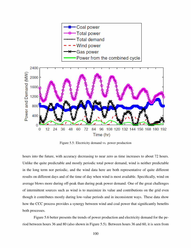
Figure 5.5: Electricity demand vs. power production
hours into the future, with accuracy decreasing to near zero as time increases to about 72 hours.
Unlike the quite predictable and mostly periodic total power demand, wind is neither predictable
in the long term nor periodic, and the wind data here are both representative of quite different
results on different days and of the time of day when wind is most available. Specifically, wind on
average blows more during off-peak than during peak power demand. One of the great challenges
of intermittent sources such as wind is to maximize its value and contributions on the grid even
though it contributes mostly during low-value periods and in inconsistent ways. These data show
how the CCC process provides a synergy between wind and coal power that significantly benefits
both processes.
Figure 5.6 better presents the trends of power production and electricity demand for the pe-
riod between hours 36 and 80 (also shown in Figure 5.5). Between hours 36 and 60, it is seen from
100

Figure 5.6 that integrated wind power is much less than that of hours 60 and 84 (approximately
50% less). The surge in wind power for the period between hours 60 and 84 would generally be
known to a dispatcher by hour 36. As indicated in the data, the amount of power produced from the
coal boiler began to decrease a few hours prior to the wind coming on line, with the energy storage
component of the CCC making up the difference until the anticipated wind power had material-
ized. The energy storage of the CCC comes from the reduced parasitic load in the coal plant, which
is not directly plotted but corresponds with the natural gas power production. In effect, the CCC
process has moved the wind power and the stored energy in the LNG tank that was filled in the
evening and night hours of the day before from a time of day when power demand is decreasing to
near the peak power demand, optimizing its value on the grid both in economic terms and in CO2
reduction. In contrast, for the period between hours 36 and 60, when wind was not significant, the
energy storage from the previous evening had to make up most of the power demand that the coal
boiler could not provide, and coal power production remained high during a longer portion of the
day.
This illustrates how the coal system with energy storing CCC can effectively move the
wind power to peak demand when it is available and can compensate for a lack of wind when it is
not sufficient, providing significant benefit to grid stability and to the economies of both systems.
While it is not shown here, wind is generally shifted forward or backward in time to the nearest
available peak in power demand, within a 24-hour window.
The LNG inventory, LNG production, and LNG requirement to run the CCC process with
the electricity price appear in Figure 5.7. Natural gas flowing to and from the pipeline and elec-
tricity price appear in Figure 5.8. In this study, LNG inventory is initialized from a non-zero value
because the integrated system of power generation and the CCC should be in operation throughout
the year. Thus, at the beginning of the simulation, a non-zero initial value is appropriately selected
for the LNG inventory, based on the pattern of this variable in subsequent days. Consequently,
until there is inventory in the tank, LNG is supplied from it (LNG underproduction in Figure 5.7).
Then, when electricity price is sufficiently cheap, natural gas is taken from the pipeline and stored
in the LNG tank. As stated before, this is also the time when electricity demand is lower than at
peak hours. Thus, LNG inventory in the tank increases (LNG overproduction in Figure 5.7) during
off peak times. It is seen in Figure 5.7 that a significant amount of natural gas is imported at hours
101

Figure 5.6: Increased value of wind power by using energy storage of the CCC
24, 72, and 144 and the tank is completely filled up. This is because of the lower average power
price at hours 24, 72, 144 than the subsequent 48 hours. After the tank is completely filled up in the
early hours of the days starting at hours 24, 72, and 144, LNG is taken from the tank and the level
of the tank drops until it reaches the low threshold of the tank. Unlike hours 24, 48, and 144, at the
beginning of hour 120 natural gas is imported as much as it can supply LNG for only the next 24
hours. Integrated wind power during the day starting at hour 120 is more than any other days in the
time horizon (with respect to the integrated electricity demand). Because wind will help meet the
demand, less LNG is needed in the tank in that day to supply sufficient cooling capacity through
the peak. For other days, the LNG tank fills completely because of less available wind and more
expensive power price.
102

Figure 5.7: LNG inventory, LNG production, and LNG required to run the CCC vs. power price
Although the maximum power required to increase the pressure of the recirculating natural
gas to the pipeline pressure is approximately 3.2 MW, it is still more economical (though not more
energy efficient) to export a fraction of the more pure natural gas to the pipeline until the electricity
price is comparatively low. In the cases where the export of natural gas is not considered an option,
the trend of other variables remain the same but the profit obtained over the entire time horizon
decreases by 16.6% when compared to cases where the export of natural gas is considered. Mixed
refrigerant compressors should also remain in operation during peak hours to process natural gas
that could have otherwise been exported to the pipeline. Therefore, more power should be produced
to meet the loss of the mixed refrigerant compressor. The aforementioned facts also illustrate the
advantage of using LNG as a refrigerant in the CCC process as it can be exported to the pipeline
103

Figure 5.8: Natural gas imported and exported vs. power price
when it is vaporized in the CCC process. Vaporized LNG also serves as a fuel when it is needed to
produce more power in the gas turbine.
It is also important to mention that the exported natural gas shown in Figure 5.8 starts
from a non-zero value at the beginning of the simulations. Similar to the LNG inventory, the
initial value of the exported natural gas is selected according to the pattern of this variable in the
following days. Because the electricity price is not sufficiently low, a fraction of the vaporized
LNG is exported to the pipeline. The export of natural gas continues until the electricity price
reaches a low value at hour 6. However, there is still LNG inventory in the tank and the hybrid
system is driven by the stored LNG until it reaches the low threshold in early hours of the next day.
Depending on the power price, this general trend in LNG inventory (Figure 5.7) and natural gas
imported and exported (Figure 5.8) cycles regularly. This is typical for an integrated system with
104

energy storage capability. This cyclical nature is based on the ongoing need for electricity which,
in return, requires natural gas and LNG for flue gas treatment in the CCC process.
Electricity on-site demand curves for the main electricity consuming components of the
system provide additional insight. The demand curves for the natural gas compressor, mixed re-
frigerant compressor, and CCC plant (Figure 5.9) illustrate the dynamics of the plant. The natural
gas compressor and CCC plant depend on the residential electricity demand because more power
should be produced during peak hours, which in turn produces more flue gas. Therefore, the CCC
plant demand also increases during peak hours. However, Figure 5.5 shows that more power is pro-
duced from natural gas during peak hours. Because natural gas combustion emits less CO2, less
LNG is required when compared to the case where coal is combusted to meet the same amount
of electricity demand. Thus, during peak hours, the natural gas compressor has lower electricity
demand than in off-peak hours when coal is the main source of power production. On the other
hand, the mixed refrigerant compressor demand decreases when electricity is expensive as most
of the required LNG is taken from the tank. This is the main energy storing aspect of CCC; the
parasitic load associated with the CCC-based carbon capture can be partially or completely met
with stored LNG. An insignificant residual flow remains to maintain spinning turbomachinery and
temperature profiles. When LNG is stored in the tank and power demand is high, it is economical
to curtail the mixed refrigerant compressor and transfer the saved electricity to meet the peak de-
mand. When there is no storage tank, power should also be supplied to compensate for the loss of
the mixed refrigerant compressor and to meet the LNG requirement during peak hours. A compar-
ison between power demand of the mixed refrigerant compressor with and without energy storage
is shown in Figure 5.10. The efficiency loss associated with working at a different load than the
designed case in the operation of the mixed refrigerant compressor is not considered in this study
and should be addressed in future work.
The average profit acquired from the integrated system is approximately $35k/hr. While
the annual performance of the hybrid system over a longer time frame is needed, it is expected
that the profit obtained from this hybrid system is sufficiently large to pay a significant fraction of
the cost of construction of the cryogenic carbon capture plant. Performance of the system over a
longer time horizon is the subject of future work.
105

Figure 5.9: Demand curves for natural gas compressor, mixed refrigerant compressor, and CCC plant
5.5.1 Sensitivity Analysis
Finally, the effects of the penalization factors applied in this study (c∆u in Equation (2.5))
are investigated. Penalization factors influence the optimization outcome and are adjustable param-
eters to obtain simulation results that are satisfactory based on operator feedback. These factors
serve as tuning factors to the model to smooth the trend of the variation of the simulated operation.
If movement penalization is not applied, large and sharp variations in the trends of variables creep
into the solution with little additional benefit towards the overall objective. This movement con-
trasts with the desired stability of the system and highlights the need to include additional terms in
the optimization problem to align simulation objectives with operational experience. However, it
is important to minimize the use of penalization factors as much as possible because they impose
106

Figure 5.10: Comparison between power demand of mixed refrigerant compressor with and without energystorage
an artificial cost to the objective function. A penalization factor is applied to the flow rate of the
imported and exported natural gas. The change in the objective function for applying different
penalty factors for these variables is less than 5% for one order of magnitude of variation. In other
words, these penalization factors do not change the overall trend of the variables over the time
horizon (not shown here), and the main effect the factors have is on the smoothness of the results.
These tuning factors are adjusted in each simulation when sharp fluctuations are observed in the
trend of the decision variables from initial attempts to solve the problem.
107

5.6 Conclusion
This chapter reports an optimization framework for the integrated system of fossil and re-
newable energy sources with the energy-storing version of the cryogenic carbon captureTM (CCC)
process. The CCC process has rapid response to the fluctuations in the electricity demand and is
able to store excess energy in the form of condensed, cold refrigerant. These features enable the
power grid to utilize more renewable energy sources. The objective in this chapter is to meet the
total electricity demand of a residential area and the CCC process and to maximize the operating
profit of the system.
Results show that a combination of coal, gas, and wind generation can be fully utilized to
meet the total electricity demand. Produced CO2 from the fossil-fueled power plants is captured at
a rate of 90% while 100% of the available wind power is utilized. The sporadic wind production is
effectively moved from periods of low value to the grid to periods of peak value while significantly
stabilizing the grid. Off-peak excess generating capacity also moves to peak periods, increasing
capital utilization and decreasing the fluctuation in boiler loads relative to the fluctuation of power
demand. While the steam boiler considered in this chapter is assumed to follow the electricity
demand curves in a change rate as much as 7% per minute, the maximum rate of load change in
the boiler is observed to be less than 0.1% per minute. The average profit acquired from the hybrid
system is approximately $35k/hr. The performance of the integrated system for baseline steam
boilers that are not able to follow the electricity demand curves is the focus of Chapter 6.
108

CHAPTER 6. DYNAMIC OPTIMIZATION OF A HYBRID SYSTEM OF CRYOGENICCARBON CAPTURE AND A BASELINE POWER GENERATION UNIT
6.1 Introduction
Integration of the CCC capture process with a coal–fired steam boiler that is able to follow
the load was considered in Chapters 4 and 5. However, many coal–fired generation units operate in
a baseline mode and the power output from those generation units is approximately constant over
most of the operational lifetime. This chapter considers the integration of a baseline coal–fired
steam boiler with a cryogenic capture process. Considering energy storage, the hybrid system is
also able to follow the peak demand with a gas turbine without necessarily cycling the coal–fired
steam boiler. This is a distinguishing feature of this chapter from Chapter 5. Minor adjustments
to the model developed in Chapters 4 and 5 make boiler output constant or load–following. This
chapter quantifies boiler cycling costs and the economic benefit of their mitigation by CCC in
systems with and without intermittent sources such as wind.
This chapter is divided into four sections. First, the adjustments required in the model
to represent the baseline performance are discussed. Next, the optimization results obtained for
an integrated system of a baseline power generation unit and the CCC process are presented. A
comparison between power production in the gas turbine through a simple or combined cycle is
also made. Finally, the impact of energy storage of cryogenic carbon capture on leveling the power
output from a steam turbine and the associated savings are discussed.
6.2 Model Adjustment for Baseline Performance
As mentioned previously, the model developed in Chapters 4 and 5 is slightly adjusted
to achieve the performance of a baseline coal–fired power generation unit. This is achieved by
dedicating a large penalization factor, c∆u in Equation 2.5a, to the variation of the set point of the
steam turbine power output, (PSP). In this case, the steam turbine power output does not vary
109

unless there is an improvement in the overall objective function. In addition, the change in steam
turbine power output between subsequent time steps is limited to 100 MW/hr to further restrict
the variation of the power output in the steam turbine. This maximum change rate is much less
than 1%/min of the nominal load–following capacity of the steam turbine.
To make the objective function more accurate, the variable and fixed operating and mainte-
nance (VOM) costs of the the power generation units are added to the profit function developed in
Equation 5.8. The variable operating and maintenance of the coal- and gas-fired power generation
units are represented by VOMCT and VOMGT while fixed operating costs (FOM) are presented by
FOMCT and FOMGT for the coal– and gas–fired power units, respectively. In this investigation,
the same VOM and FOM costs are assumed for both power generation types and are equal to 7.3
and 10.2 dollar per MWh of energy production, respectively [166]. Thus:
Pro f it = (DRes−DPlant)PE − (NGPL−NGEXPT )PN−PCC
−(FOMCT +VOMCT )PCT − (FOMGT +VOMGT )PGT(6.1)
The input data and other assumptions used to evaluate the performance of an integrated
system with a baseline coal–fired generation unit are the same as a load–following unit discussed
in Chapter 5.
6.3 Results and Discussion
The results for the integration of cryogenic carbon capture with a baseline coal–fired power
plant are presented in this section. Figure 6.1 presents the total power generation in the steam
turbine. For comparison, the power generation from a load-following steam turbine is also shown
in Figure 6.1.
As is observed in Figure 6.1, total power generated in the steam turbine does not vary
significantly for most of the simulation time. The minimum output for the steam turbine (820
MW ) is close to the selected lower limit (800 MW ). Because the steam turbine operates as a
baseline unit, the power output from this unit does not cycle during peak hours and gas power is
used instead as the peaking unit (shown in Figure 6.2). The small variations observed in the trend
110

Figure 6.1: Total power generation from the steam turbine vs. wind power
of the steam turbine power output between hours 110 and 160 is because of a high penalization
factor, whi, dedicated to avoid overproduction of power. When wind power is significant (for
instance for the period between hours 115 to 150), power output from the steam turbine decreases
a few hours before the wind power comes online with the energy storage component of the CCC
process making up the difference. Thus, the cost associated with power overproduction is avoided.
While this small variation is inevitable to avoid the overproduction penalization cost, the power
output remains constant after the change is made as a result of the penalization cost associated
with variation of power output of the steam turbine. It is also observed that after hour 156 to
the end of the simulation time, wind power has a smaller contribution in meeting the electricity
demand and it is found more economical to increase the power output from the steam boiler.
From Figure 6.2, it is also observed that the overall electricity demand is met through a
combination of power sources. Whenever wind power is available, it is utilized first to meet the
electricity demand while the power output of the steam turbine is mostly at a value close to the
111

Figure 6.2: Electricity demand and power production from coal, wind, and natural gas
minimum residential electricity demand. Gas power is mostly produced during peak hours to meet
the increasing electricity demand. This is because more LNG is required in the CCC process to
treat the higher amounts of flue gas produced during these hours. As LNG from the tank produces
excess natural gas inside the plant (after treating the flue gas), this natural gas could be used for
power generation in the gas turbine. This is more economical than combusting coal to meet the
peak demand. This finding is also compatible with the baseline nature of the steam turbine and
permits the optimization problem to avoid the cycling cost of the steam turbine. Production of
gas power is a direct impact of using energy storage; i.e. it permits the system to overproduce
LNG refrigerant during low power demand or when wind is readily available and to drive the CCC
process from the stored refrigerant. The excess warm refrigerant produced during energy recovery
is either sent back into the pipeline or used as a fuel source in a gas turbine.
From Figure 6.2, it seems that a value of 1020 MW , the maximum output from the steam
turbine, is reasonable to meet the combined electricity demand of the residential users and CCC
plant. However, economical calculations are needed with consideration of the life time of the
steam turbine and the growing need in electricity demand to accurately size it. While with the
energy storage capability of the CCC process it is expected to benefit wholesale electricity prices
112

in a power grid, no impact on the energy price is assumed. The output results obtained from
such analysis predict the required energy from each source for the following days subject to the
constraints for each power source (e.g. baseline steam turbine). The impact of the energy storage
on the wholesale electricity prices is outside the scope of this study.
Trends of variables for the natural gas imported and exported to the plant are shown in
Figure 6.3a and are similar to the results obtained in Chapter 5. Import of natural gas to the plant
is mainly observed when electricity is cheap. Export of natural gas from the plant, on the other
hand, occurs when electricity is relatively expensive. This permits the system to avoid liquefying
the circulating natural gas (NGCCC) when demand in electricity is high. Trends of LNG inventory
in the tank (Figure 6.3b) reflect an excellent transient response of this optimization problem to
fluctuations in residential demand, energy price, and wind power availability. LNG inventory in
the tank is dependent on the energy price, current inventory in the tank, wind power availability,
and the penalization factors used for the natural gas imported to and exported from the plant. Thus,
LNG inventory is a cumulative effect of these factors and is less intuitive to accurately attribute its
trend to each of these factors. However, it is expected to store LNG when higher electricity price
or lower wind availability are foreseen. For instance, between hours 86 and 92 when two peaks
in electricity price are anticipated, LNG is stored in the tank before reaching hour 86 to be used
during this period. Recovery of the LNG from the tank continues until the tank is emptied at hour
124. LNG storage is started again after hour 125; however, more wind power is available from
hour 123 to 144 and the tank is not filled completely. This is because the increased availability
of wind power is utilized to meet the power demand and less power is produced from the fossil
fuels (consequently less CO2 is produced). After hour 152, on the other hand, wind power is less
available and it is seen that the LNG tank is fully filled before reaching hour 152. A reasonable
cycling in the trend of LNG inventory is also observed after hour 152 and in the first 72 hours.
These findings are also similar to the performance of the integrated system with a load–following
coal–fired power plant.
While the penalization factors are used to smooth the trends of variations in natural gas to
and from the plant, the overall trends for these variables and LNG inventory remain the same; i.e. a
cyclical trend for the LNG inventory is observed and import and export of natural gas occur during
off and on peak hours, respectively.
113

(a) Natural gas imported to and exported from theplant (b) LNG inventory
Figure 6.3: Trend of natural gas and LNG inventory
Trends of electricity demand for the mixed refrigerant (MR) and natural gas (NG) com-
pressors are presented in Figure 6.4. A peak in the electricity demand of the mixed refrigerant
is observed during off–peak hours that is associated with the storage case when the LNG tank
is filled. The CCC process is then operated with the LNG recovered from the tank and permits
the mixed refrigerant compressor to work at a minimum load when electricity is in high demand.
Reduction in the electricity demand of the mixed refrigerant compressor can continue for as long
as there is LNG inventory in the tank. Decisions on how long either energy storage or recovery
should continue are economically-driven. As discussed in Chapter 5, inefficiency associated with
working at non–optimal operating points for the compressor is not considered and the compressor
is also permitted to turn on and off without any efficiency penalty. While these assumptions are
acceptable to convey the energy storage concept, they should be modified when financial decisions
are made. This is the focus of future work.
The average profit obtained from Equation 6.1 for a baseline steam turbine over the se-
lected days is $6.5k/hr. This is compared to $13.6k/hr obtained when the power output from the
steam turbine is allowed to vary without penalization. When the steam turbine is allowed to vary,
penalization factor for the variation of power output, c∆u in Equation (2.5a), relaxes; thus, the hy-
brid system obtains a new optimum and results in an average profit of $13.6k/hr. The ratio of total
profit and total energy production from all sources considered over the simulation time is 0.43
114

Figure 6.4: Electricity demand for refrigeration compressors and CCC plant in a combined cycle powergeneration unit with energy storage
¢/kWh for a baseline case while it is 0.91 ¢/kWh for a variable steam turbine. When fixed and
variable operating and maintenance costs of the coal– and gas–fired power generation units (VOM
and FOM) are ignored in Equation (6.1), the average profit for the baseline case is approximately
$29k/hr which is 20% less than the average profit of a load-following steam turbine ($35.5k/hr).
Similarly, the ratio of the total profit and total energy production when VOM and FOM are ignored
in Equation (6.1) is 1.92 ¢/kWh and 2.40 ¢/kWh for baseline and load-following steam turbines,
respectively.
6.4 Comparison Between Combined and Simple Cycles
A comparison is also made when power generation from the gas turbine is achieved in a
simple cycle (scenario 1); i.e. gas turbine exhaust does not generate power. In addition, natural gas
supply for the gas turbine in scenario 1 is not the vaporized LNG exiting from the CCC process. In
115

this case, the gas turbine serves as an independent peaking unit. However, it is still assumed that
the CCC process treats the flue gas generated from the natural gas turbine. Because a simple cycle
is assumed, treatment of the gas turbine exhaust is achieved by adding it to the coal exhaust after
the coal superheaters and reheaters. The capacity of the gas turbine in scenario 1 is assumed the
same as the analysis discussed in Section 6.3 (1000 MW ). The analysis discussed in Section 6.3 is
referred to as scenario 2 for the remainder of this section. In scenario 2, the baseline performance
is achieved through a combination of the steam generated from the coal and natural gas flue gas;
i.e. when coal power in Figure 6.2 is at a maximum, power from the combined cycle is at a
minimum and the reverse trend is also observed. In scenario 1, however, the baseline performance
is achieved merely from the steam generated from coal combustion (coal power). Thus, more
coal is combusted in the steam boiler in a simple cycle to achieve the same steam flow rate and
power output as a combined cycle. To make a fair comparison, it is assumed that the power output
obtained in scenario 2 for the steam turbine, PST in Equation 4.1, is an input to scenario 1 and it is
not varied; i.e. rate of steam production is the same for both scenarios. In addition, it is assumed
in scenario 1 that energy storage is not available. This case represents a typical power generation
unit that is equipped with a carbon capture technology (without storage capability) and a peaking
unit to capture the CO2 emissions while meeting the electricity demand.
With these assumptions, optimization of the system presented in scenario 1 is implemented
and the results are compared with scenario 2. In both scenarios, power production from coal and
gas is considered a single generation unit and the power supply is used to meet the electricity
demand of residential users and the CCC plant. Figure 6.5a and 6.5b represent the trends of excess
power production in each scenario. In scenario 1, power supply equals the electricity demand
for most of the simulation time. However, both over production and under production of power
occur (Figure 6.5a) despite the penalization factors applied to balance the demand and supply of
electricity. For scenario 2, there is no mismatch between electricity demand and power supply over
the horizon. The mismatches seen in scenario 1 stem in large part from the increased power demand
on the system associated with carbon capture with no compensating increase in capacity. These
would become more severe for other carbon capture systems, essentially all of which consume
significantly more energy than CCC. The mismatches in scenario 1 are rare, however, when a grid
analysis is implemented (due to the presence of peaking units). This comparison highlights the
116

(a) Simple cycle power generation without energystorage (Scenario 1)
(b) Combined cycle power generation with energystorage (Scenario 2)
Figure 6.5: Excess power comparison between combined and simple power generation cycles with andwithout energy storage, respectively
importance of energy storage of the CCC process. Energy storage adds flexibility to a single coal–
fired generation system to operate as a baseline unit and still be able to meet the peak electricity
demand without heavily relying on other generation units in the grid. This is because the hybrid
system has a higher power production capacity through time–shifting of the compressor demand
and the combined cycle, thereby creates less severe peaking problems comparing to other carbon
capture processes.
The overall mass flow rate of the coal combusted for steam production in a system that
includes natural gas in a simple cycle is 8% more than if natural gas is in a combined cycle,
as expected. Total electricity consumption of the plant is also 8% more in scenario 1. This is
because scenario 1 produces more flue gas from coal consumption to achieve the same steam
flow rate as in scenario 2. Unlike scenario 2, the total flow rate of natural gas imported and
exported to the pipeline in scenario 1 is zero because there is no opportunity for arbitrage of
electricity without energy storage (Figure 6.6) and time–shifting of the electricity demand of mixed
refrigerant compressor is not achievable. Thus, natural gas consumption in the simple cycle power
generation unit is merely for the purpose of meeting the peak total electricity demand. In contrast,
in the case of a combined cycle with energy storage, natural gas has the dual purposes of serving
as the refrigerant and a fuel. Thus, natural gas is imported and exported from the plant to take
117

Figure 6.6: Electricity demand for refrigeration compressors and CCC plant in a simple cycle power gener-ation unit without energy storage
advantage of the arbitrage of electricity (Figure 6.4). A comparison between the profitability of
these two scenarios is meaningless because the primary goal of meeting the electricity demand at
all time steps over the horizon is not achieved in scenario 1.
6.5 Comparison of Cycling Costs
An important aspect of power plant operation is the cost associated with ramping, also
known as load following or cycling. The changes in operational levels of the plant result in in-
creased thermal, pressure, and mechanical related stress and fatigue [184, 185]. This leads to
increased equipment degradation and associated operation and maintenance costs, as well as de-
creased thermal efficiency.
In general, research done on ramping in power plants has looked at the most fragile part
of the plant, the turbine rotor. Historically unit commitment models with economic dispatch have
118

incorporated fixed ramp-rate constraints with the assumption that ramping between the constraints
will not cause damage to the turbine rotor [186, 187]. In 2012, a report published by National
Renewable Energy Laboratory [173] investigated the cost of ramping for an entire plant by consid-
ering the cycling costs of several power generation types [188]. This report provides a lower bound
for the cycling costs of eight types of generation units. The cycling costs are reported for different
cycling scenarios including cold start, warm start, hot start, and load-following cases. Between
these cycling scenarios, cold start and load-following have the highest and lowest cycling costs,
respectively. For instance, the lower bound for the cold start cycling costs of a typical large-scale
subcritical coal-fired power plant is $105/MW capacity per cycle while load-following cycling cost
for the same generation type is $2.45/MW capacity per cycle [188]. While startup scenarios im-
pose the most expensive cycling costs of the power plants, it is not the scope of this dissertation
to investigate them. Consideration of such scenarios requires a longer simulation time (e.g. one
year) to be taken into consideration. Instead, this analysis considers just the impact of cryogenic
carbon capture on the cycling costs due to load-following of the coal- and gas-fired power gen-
eration units. According to [188], the cycling cost of a generation unit varies between individual
plants and the numbers provided in this report are generic lower bounds. In this study, estimated
multiplicative factors are also provided for faster ramp rate. These multiplicative factors, however,
are not considered in this dissertation and the cycling costs are the median capital and mainte-
nance costs of typical ramping rates. This investigation considers the load-following cycling costs
of large–scale, subcritical coal–fired and natural gas combined cycle (NGCC) power generation
units. Accordingly, the cycling cost associated with load-following of a coal–fired generation unit
is $2.45/MW capacity per cycle while it is $0.64/MW capacity for a NGCC power plant. To calcu-
late the number of cycles for power generation from both coal and gas, a post–processing approach
is considered, i.e., power outputs from solving the optimization problem are used as input to the
rainflow cycle counting algorithm [189] where the output from the algorithm is the number of cy-
cles. This calculation assumes that power output from the optimization results has a similar trend
to overall stresses in the boiler. The rainflow algorithm allows the application of Miner’s rule to
assess the fatigue life of a structure subject to complex loading. More details about the rainflow
algorithm are available in [190].
119

With the abovementioned assumptions, the cycling costs of the baseline and load–following
steam turbines are considered. The power outputs from the coal– and gas– fired generation units,
PST and PGT , for both scenarios are used in the rainflow cycle counting software developed in
[191]. Consequently, the number of cycles for the load–following scenario for the coal– and gas–
fired generation units are found to be 20 and 17, respectively, over 8 days of simulation time.
For a baseline scenario, there are 1 and 21 cycles in the power output from the coal– and gas–
fired generation units, respectively. Optimization of the baseline and load-following coal–fired
generation units result in a maximum power output of 1020 MW and 1210 MW , respectively.
As mentioned previously, sizing of the generation units is beyond the scope of this dissertation
and requires extensive study. However, a capacity of 1800 MW (upper bound for PSP) is a good
estimate for both load–following and baseline coal–fired generation unit for the purpose of cycling
costs comparison. With this capacity, the cycling costs of the coal–fired unit for the load-following
scenario are 1800×2.45×20 = $88200 for 8 days of simulation time while they are 1800×2.45×
1= $4410 for a baseline case study. In addition, the cycling cost of the load–following scenario for
the gas–fired unit is 1000×0.64×17= $10880 compared to a value of 1000×0.64×21= $13440
for a baseline case over 8 days of simulation. In summary, the total costs associated with the cycling
of all generation units considered in this investigation are $99080 and $17850 for load–following
and baseline scenarios, respectively, over 8 days of simulation time. The total costs of cycling
for the same power generation units in the absence of wind power are $94100 and $14010 for the
load–following and baseline coal–fired generation unit, respectively. These costs are based on 1
and 15 cycles for the coal– and gas– fired generation units, respectively, in a baseline case while
18 and 23 cycles are observed for the the same units, respectively, in a load–following case. Table
6.1 summarizes these results.
The saving in the cycling costs of the baseline generation units, in the presence and absence
of wind power, is also a direct result of the energy storage of cryogenic carbon capture. It is well–
known that coal–fired generation units are mainly designed for baseline operation. Equipping
the coal–fired power plant with cryogenic carbon capture enables the power generation unit, as a
whole, to follow the load without necessarily varying the steam turbine output. This is achieved by
supplying the natural gas required for the peaking unit from the storage system while the carbon
dioxide separation from both generation units remains in operation.
120

Table 6.1: Summary of cycling costs
With wind Without windLoad-following
boilerBaseline
boilerLoad-following
boilerBaseline
boilerNo. Cycles in boiler
(Cost)20
($88200)1
($4410)18
($79380)1
($4410)
No. Cycles in gas turbine(Cost)
17($10880)
21($13440)
23($14720)
15($9600)
Total cycling costs $99080 $17850 $94100 $14010
It should be emphasized that these costs are the generic lower bounds for cycling of the
power generation units, and they do not consider the more expensive practices of cold, warm, and
hot starts. In addition, it is unlikely to have this many cycles in the boiler in 8 days to follow the
load in practice (for both baseline and load–following power generation units). This is because
supplemental peaking units are used to avoid the variations in power output from the coal–fired
generation units. While more accurate analysis of the number of cycles requires longer simulation
horizon, this study demonstrates the potential reduction in cycling costs of a coal–fired power
generation unit by utilizing the energy storage of the CCC process.
6.6 Conclusion
This chapter considers dynamic integration of a baseline fossil–fueled power generation
unit with cryogenic carbon capture. Similar to the integrated system with load–following capabil-
ity (discussed in Chapter 5), effective time–shifting of the electricity demand of the refrigeration
compressors is observed for a baseline case study. The total electricity demand of the residential
users and the CCC plant is met through a combination of power sources. Wind power, whenever
available, is first used in meeting the demand. This leads to 100% utilization of the wind power.
With the energy storage of cryogenic carbon capture, a single coal–fired generation system is able
to operate as a baseline unit and still be able to meet the peak electricity demand. Energy stor-
121

age also enables a potential 82% and 85% decrease in the costs associated with load–following of
power generation units in presence and absence of wind power, respectively.
122

CHAPTER 7. CONCLUSION AND FUTURE WORK
7.1 Conclusion
Increasing demand of energy has motivated ongoing optimization of the new and existing
technologies. In this dissertation, advanced estimation, optimization, and control techniques are
applied to representative applications of large–scale and complex systems. The methods enhance
the profitability and product quality while minimizing energy consumption. Moving horizon esti-
mation and model predictive control are utilized in this study to optimize mathematical models of
a batch distillation column and a hybrid system of power generation and cryogenic carbon capture.
The estimation and control frameworks developed for both applications are modular and applica-
ble to optimize complex dynamic systems. These models are nonlinear and non–convex. Several
strategies are developed in Chapter 2 to initialize the nonlinear models and find a successful so-
lution with improved computational time and convergence properties. Convergence is improved
through a methodology to break a larger problem down into separate parts that can be isolated and
diagnosed for convergence issues.
In Chapter 3, shortcut-based and detailed mathematical models are developed for a batch
distillation column. This model utilizes a dynamic parameter estimation approach with an `1-norm
objective function to fit the model prediction to experimental data. Data collection from the dis-
tillation column is achieved by applying a doublet test on the column reflux ratio and measuring
the instantaneous composition and molar quantity of methanol. With dynamic parameter estima-
tion, system non-idealities are included in the model to capture a high fidelity model response and
compare it with a reduced–order model. Dynamic parameter estimation with a sensitivity analy-
sis reduces the experimental data requirement from the column by identifying key parameters for
identification. The accuracy of the estimated parameters is verified by implementing a nonlinear
statistical analysis. The results predicted by the reduced–order model developed in this dissertation
match the experimental data and the results obtained from a more rigorous first–principles model.
123

The solution time of the simplified model is, however, 5-10 times faster than the first-principles
model. Faster solution time of the model is desirable in real-time control and online optimization
applications. The verified model is then used to optimize the column operation by manipulating
the column reflux ratio. Similar to the estimation analysis, an `1-norm objective function is utilized
for column optimization. With dynamic optimization of the column, a 14% increase in methanol
production is observed while the product composition meets the final purity requirements. With-
out measurement feedback, the predictions from the optimization analysis match the experimental
data with a maximum error of 10% and 0.8% for overall methanol production and composition,
respectively.
In a second application of the methodology for large–scale and complex systems, an opti-
mization framework for a hybrid system of power generation and the CCC process is developed.
The CCC process considered in this investigation is a novel technology for CO2 removal from the
flue gases of fossil–fuel power plants. Benefits are lower energy consumption, rapid response to
fluctuations in demand, increased adoption of intermittent power supplies, and grid–scale energy
storage capability. This study considers the dynamic integration of a simulated coal–fired power
plant with cryogenic carbon capture for the first time. In this dissertation, data provided by the
Sustainable Energy Solutions for energy demands, response times, and energy storing capabilities
is used to analyze the impact of the CCC process on the power grid. The two main goals of this
analysis are: (1) meet the total electricity demand and (2) maximize the operational profit of the
hybrid system while capturing 99.9% of the CO2. The modeling framework developed in this dis-
sertation is modular; i.e. different capture processes, energy storage, and power generation units
can be considered in this framework to explore several adoption and integration scenarios that lead
to increased grid stability and full utilization of renewable sources. Three main case studies are
considered for the hybrid system: (1) a load–following boiler without energy storage, (2) a load–
following boiler with energy storage, and (3) a baseline boiler with energy storage. The analysis
for a baseline boiler with natural gas peaking turbines addresses the operation of older designs
of coal–fired power generation units while operation of recently designed coal power plants is
highlighted in the load–following boiler analysis.
For the case study without energy storage, it is shown that power demand is always met
through a combination of coal, gas, and wind power (for both summer and winter case studies).
124

For the winter case, wind power is more readily available and it has a stronger contribution to the
total electricity demand. However, because of the high fluctuations in wind power availability, gas
power is favored relative to the summer case. This is because of the rapid response of the gas
power to make up for the intermittent behavior of wind power. Increased production of power
from the natural gas in winter case requires more fuel that should be imported from the pipeline.
Consequently, 100% increase in the overall intake of natural gas for the winter case, in comparison
to the summer case, is observed. The overall production of LNG as stored refrigerant for the CCC
process decreases by 80% in the winter case. This is because the higher share of power production
from wind and natural gas reduces the total CO2 production. Thus, less refrigerant is required
for flue gas treatment. The average operational profits for the summer and winter case studies
are $21k/hr and $13k/hr. The higher profit obtained in the summer case is attributed to the larger
variation in the electricity price than the winter case. A sensitivity analysis for the impact of wind
power adoption in meeting the demand is a novel contribution of this work. With an increase in
the adoption rate of wind power, power production from coal decreases while power generation
from natural gas increases. The trade-off between a decrease in coal consumption and an increase
in natural gas consumption results in a maximum in the trend of profitability with respect to wind
adoption rate; i.e. at a value of α = 0.66, the profit of the hybrid system without energy storage is
at a maximum. This observation remains valid for a range of natural gas and coal prices.
Energy storage significantly improves the performance of a hybrid system. When energy
storage is included, import of natural gas shifts to time periods with a low electricity price. This
also causes a peak in the LNG production (and electricity demand of the refrigeration compressor)
to shift to these time periods. The LNG produced in excess during these times accumulates in
an insulated vessel and is utilized when electricity demand and price are high. This curtails the
electricity demand of the refrigeration compressor during peak–hours. Export of natural gas to
the supply pipeline during peak hours further reduces the demand of the refrigeration compressor.
Effective time–shifting of this compressor work (and LNG inventory in the tank) occurs for both
load–following and baseline scenarios. This work also demonstrates the enhanced contribution of
wind power by utilizing large-scale energy storage of the CCC process. A profit of $35.5k/hr and
$29k/hr is obtained from optimization of the load–following and baseline power plants, respec-
tively (ignoring the FOM and VOM costs). These profits are equivalent to 2.4 ¢/kWh and 1.92
125

¢/kWh for the load–following and baseline power plants, respectively. The profit obtained from
dynamic optimization of the hybrid system can pay a significant fraction of the cost of construction
and operation of the cryogenic carbon capture plant, the latter being estimated at 2.5-3 ¢/kWh.
Similar to the case without energy storage, total power demand is met through a combina-
tion of power sources. In all scenarios, wind power is utilized first to meet the electricity demand.
Gas power is mainly produced during peak hours or when wind varies significantly. The fuel sup-
ply for the gas turbine is either from the pipeline (without energy storage) or when an LNG storage
tank is available. Coal remains the main source of power production in this hybrid system.
A comparison is also made between the operation of a combined cycle and a simple cycle
power generation unit. In the simple cycle, the gas turbine operates as an independent peaking
unit and the fuel supply for the turbine is not from energy storage (unlike the combined cycle).
While the rate of steam production is assumed the same for both scenarios, energy storage is not
considered in the simple cycle scenario. Thus, the simple cycle represents a typical coal–fired
power plant that is equipped with a carbon capture process without energy storage. Optimization
results show that when energy storage is not considered, significant mismatches between power
production and demand occur throughout 8 days of simulation time. This highlights the importance
of energy storage of the CCC process. With energy storage, the hybrid power generation unit is
capable of producing more power during peak hours, thereby the CCC process creates less severe
peaking problems comparing to other carbon capture processes.
Total cycling costs of all generation units potentially decreases by 82-85% with baseline
operation. Equipping the power generation unit with large–scale energy storage of the CCC process
stabilizes the baseline production. It enables the hybrid system to follow the load while CO2
capture remains in operation and the output power of steam turbines do not vary significantly.
7.2 Future Work
Several future contributions are needed to further enhance capabilities to solve large–scale
and complex dynamic systems. One important area is the development of mixed–integer nonlinear
programming solvers to achieve faster solution times and higher success rates in finding a solution
(or to quickly identify infeasible problems). In addition to enhanced algorithm development, sev-
126

eral innovations are proposed for batch distillation and integrated energy systems in the following
two sections.
7.2.1 Batch Distillation Column
The model developed for the batch distillation column is optimized in an offline mode.
Application of the model for online optimization of the column would improve performance by
utilizing measurement feedback to continually correct model predictions and re–plan the batch
reflux ratio profile. A nonlinear confidence interval for `1-norm objectives has not been fully
developed because the F–statistic is based on the ratio of χ2 distributions. The χ2 distributions
are currently only for squared error objectives. Application of this approach for advanced column
designs such as a cyclic distillation column is another potential direction for future work.
7.2.2 Hybrid System of Power Generation and the CCC Process
The effects of equipment capital cost in the economic evaluation of the integrated system
are not considered in this investigation. Considering capital costs of the equipment in economic
evaluation of the hybrid system requires a longer simulation horizon. This issue should be ad-
dressed in future work because sizing of equipment influences the dynamic operation and overall
profitability. In addition, operation of the refrigeration compressor at different operating points is
assumed to have the same efficiency. The efficiency loss due to operation at non–optimal points
is the focus of future work. Additionally, compressors have finite turndown ratios and a minimum
flow is typically circulated in the compressor to avoid shutting down the compressor completely.
This should be added to the model in future analysis. Moreover, there is a significant cost as-
sociated with operating a boiler at a power output less than its designed capacity. For example,
cyclic operation of a boiler is an instance that leads to a lower capacity utilization. This results
in an increase in the average cost of power generation. Considering the impact of operating the
boiler at a reduced power output on the cost of power generation is the focus of future work. Ad-
ditionally, not all natural gas is suitable for LNG storage. The CO2 content of natural gas might be
higher than the LNG production standards. The CCC process can also be used to reduce the CO2
content from the pipeline natural gas. The natural gas processing facility is discussed in details
127

in [192–194]. Integration of the natural gas processing facility with the hybrid system of power
plant and the CCC process is another direction for future work. Further future directions include
investigating the impact of the recirculation system on the flue gas exhaust from coal and gas–fired
power plants, quantifying the impact of the energy storage on the wholesale electricity prices, con-
sidering the more expensive start–up scenarios on cycling costs of the power plants, and exploring
the uncertainty in prices and wind data.
The impact of cryogenic carbon capture along with the associated energy storage is con-
sidered on a single power generation unit. The energy storage of the CCC process can positively
impact the stability of the power grid. In current power grid systems, stability and reliability of the
grid depend in part on the individual unit availability and in part on spinning reserves. Spinning
reserves are typically operated when there is a sudden increase in electricity demand or when some
other generation unit unexpectedly goes off line. Because this only occasionally happens, spinning
reserves typically have very low capacity factors, which in turn leads to very high average cost
of power generation. The cost of power generation as a function of the cumulative grid operating
capacity forms a dispatch curve similar to Figure 7.1 with the low capacity-factor systems typically
having the highest costs [195]. The cost curve is highly nonlinear with peaking plant sources. What
the figure does not illustrate is that some amount of spinning reserve is always online, regardless
of the overall grid demand. Therefore, the rapid increase in cost of power for the last increment
of capacity will always exist, regardless of the power demand. The systems represented by this
section of the curve generally only operate during high or sudden increase in power demand. This
gives rise to significant changes in the cost of power generation from low to high demand periods.
These differences are an inherent part of any highly reliable grid that integrates several individ-
ual power sources. The energy storage portion of CCC, however, can effectively become the grid
spinning reserve by adjusting the parasitic load of the compressors in time to accommodate the
dispatch schedule of the grid. This energy storage capacity will essentially always have significant
economic benefit on a grid. Simulation of a larger power grid with fossil-fueled units equipped
with CCC is the scope of future work.
Additionally, the abovementioned optimization framework for the power grid should be
implemented in an actual dispatch control center for a grid. This framework is required to consider
real-time updating of the model with respect to operational changes or disturbances in the grid.
128

Figure 7.1: Power supply curve for Southeastern Electric Reliability Council region [195]
This is especially important for unpredictable upsets in the grid such as the shut down of a power
plant on the grid. This requires addition of more robust optimization algorithms, utilization of
warm-start initialization strategies, and usage of more computational resources.
7.3 Publications
The main contributions of this dissertation are presented in several journal papers and con-
ferences and they are listed below:
• Safdarnejad, S.M., Hedengren, J.D., Baxter, L.L., Dynamic Optimization of a Hybrid Sys-
tem of Energy–Storing Cryogenic Carbon Capture and a Baseline Power Generation Unit,
Applied Energy Journal, Volume 172, Pages 66-79 (Chapters 4 and 6)
• Safdarnejad, S.M., Gallacher, J, Hedengren, J.D., Dynamic Parameter Estimation and Op-
timization for Batch Distillation, Computers and Chemical Engineering Journal, Volume 86,
Pages 18-32 (Chapter 3).
129

• Safdarnejad, S.M., Hedengren, J.D., Lewis, N.R., Haseltine, E., Initialization Strategies for
Optimization of Dynamic Systems, Computers and Chemical Engineering Journal, Volume
78, Pages 39-50 (Chapter 2).
• Safdarnejad, S.M., Hedengren, J.D., Baxter, L.L., Plant-level Dynamic Optimization of
Cryogenic Carbon Capture with Conventional and Renewable Power Sources, Applied En-
ergy Journal, Volume 149, Pages 354-366 (Chapter 5).
• Safdarnejad, S.M., Kennington, L., Hedengren, J.D., Baxter, L.L., Investigating the Im-
pact of Cryogenic Carbon Capture on the Performance of Power Plants, American Control
Conference (ACC), Chicago, IL, July 2015 (Chapter 4).
• Safdarnejad, S.M., Richards, J., Griffiths, J., Hedengren, J.D., Baxter, L.L., Increased Sta-
bility of a Power Grid by Energy Storage of Cryogenic Carbon Capture, AIChE Spring
Meeting, Houston, TX, Apr. 2016 (Chapter 6).
• Safdarnejad, S.M., Gallacher, J. R., Hedengren, J.D., A New Framework for Dynamic Pa-
rameter Estimation and Optimization of Batch Distillation Columns, AIChE National Meet-
ing, Salt Lake City, UT, Nov. 2015 (Chapter 3).
• Safdarnejad, S.M., Hedengren, J.D., Baxter, L.L., Reduction in Cycling of the Boilers by
Using Large-Scale Energy Storage of Cryogenic Carbon Capture, AIChE National Meeting,
Salt Lake City, UT, Nov. 2015 (Chapter 6).
• Safdarnejad, S.M., Hedengren, J.D., Baxter, L.L., Dynamic Optimization of the Hybrid
System of a Baseline Power Generation Unit and Cryogenic Carbon Capture, Western States
Section of the Combustion Institute, Provo, UT, Oct. 2015 (Chapter 6).
• Safdarnejad, S.M., Hedengren, J.D., Baxter, L.L., Effect of Cryogenic Carbon Capture
(CCC) on Smart Power Grids, AIChE Spring Meeting, Austin, TX, Apr. 2015 (Chapter 6).
• Safdarnejad, S.M., Hall, T., Hedengren, J.D., Baxter, L.L., Dynamic Optimization of Cryo-
genic Carbon Capture with Large-scale Adoption of Renewable Power, AIChE National
Meeting, Atlanta, GA, Nov. 2014 (Chapter 5).
130

Bibliography
[1] Manenti, F., Lima, N. M., Lian, L. Z., Cuoci, A., and Frassoldati, A., 2010. “General-ized classes for lower levels of supply chain management: Object-oriented approach.” In20th European Symposium on Computer Aided Process Engineering, S. Pierucci and G. B.Ferraris, eds., Vol. 28 of Computer Aided Chemical Engineering. Elsevier, pp. 139 – 144. 9
[2] Buzzi-Ferraris, G., and Manenti, F., 2014. Differential and Differential-Algebraic Systemsfor the Chemical Engineer: Solving Numerical Problems. Wiley, New York. 9
[3] Sun, L., Hedengren, J. D., and Beard, R. W., 2014. “Optimal trajectory generation usingmodel predictive control for aerially towed cable systems.” Journal of Guidance, Control,and Dynamics, 37(2), pp. 525–539. 9, 32, 43
[4] Kumar, A., and Daoutidis, P., 1999. Control of nonlinear differential algebraic equationsystems. Chapman & Hall/CRC, New York. 9
[5] Biegler, L. T., 2007. “An overview of simultaneous strategies for dynamic optimization.”Chemical Engineering and Processing: Process Intensification, 46(11), pp. 1043 – 1053. 9
[6] Biegler, L., Campbell, S., and Mehrmann, V., 2012. Control and Optimization withDifferential-Algebraic Constraints. SIAM - Society for Industrial and Applied Mathematics,Philadelphia. 9
[7] Carey, G., and Finlayson, B., 1975. “Othogonal collocation on finite elements.” ChemicalEngineering Science, 30, pp. 587–596. 9
[8] Renfro, J., Morshedi, A., and Asbjornsen, O., 1987. “Simultaneous optimization and so-lution of systems described by differential/algebraic equations.” Computers and ChemicalEngineering, 11(5), pp. 503 – 517. 9, 43
[9] Liebman, M., Edgar, T., and Lasdon, L., 1992. “Efficient data reconciliation and estimationfor dynamic processes using nonlinear programming techniques.” Computers and ChemicalEngineering, 16, pp. 963–986. 9
[10] Albuquerque, J. S., and Biegler, L. T., 1995. “Decomposition algorithms for on-line esti-mation with nonlinear models.” Computers and Chemical Engineering, 19, pp. 1031–1039.9
[11] Cervantes, A., and Biegler, L., 1998. “Large scale DAE optimization using simultane-ous nonlinear programming formulations.” SIAM Journal on Numerical Analysis, 44(5),pp. 1038–1050. 9
[12] Hong, W., Wang, S., Li, P., Wozny, G., and Biegler, L., 2006. “A quasi-sequential approachto large-scale dynamic optimization problems.” AIChE Journal, 52, pp. 255–268. 9
131

[13] Mıguez, J., 2010. “Analysis of a sequential monte carlo method for optimization in dynam-ical systems.” Signal Processing, 90(5), May, pp. 1609–1622. 9
[14] Binder, T., Blank, L., Bock, H., Burlisch, R., Dahmen, W., Diehl, M., Kronseder, T., Mar-quardt, W., Schloder, J., and Stryk, O., 2001. Online Optimization of Large Scale Systems.Springer-Verlag Berlin Heidelberg, ch. Introduction to model based optimization of chemi-cal processes on moving horizons, pp. 295–339. 9
[15] Diehl, M., Bock, H. G., Schloder, J. P., Findeisen, R., Nagy, Z., and Allgower, F., 2002.“Real-time optimization and nonlinear model predictive control of processes governed bydifferential-algebraic equations.” Journal of Process Control, 12, pp. 577–585. 9
[16] Assassa, F., and Marquardt, W., 2014. “Dynamic optimization using adaptive direct multipleshooting.” Computers and Chemical Engineering, 60(0), pp. 242 – 259. 9
[17] Leppavuori, J. T., Domach, M. M., and Biegler, L. T., 2011. “Parameter estimation in batchbioreactor simulation using metabolic models: Sequential solution with direct sensitivities.”Industrial and Engineering Chemistry Research, 50(21), pp. 12080–12091. 9, 43
[18] Brenan, K. E., Campbell, S. L., and Petzold, L. R., 1996. Numerical solution of initial-valueproblems in differential-algebraic equations., Vol. 14 SIAM. 10
[19] Ascher, U. M., and Petzold, L. R., 1998. Computer methods for ordinary differential equa-tions and differential-algebraic equations., Vol. 61 SIAM. 10, 22
[20] Petzold, L. R., 1982. Description of dassl: A differential/algebraic system solver Tech. rep.,Sandia National Labs., Livermore, CA (USA). 10
[21] Hindmarsh, A. C., Brown, P. N., Grant, K. E., Lee, S. L., Serban, R., Shumaker, D. E., andWoodward, C. S., 2005. “SUNDIALS: Suite of nonlinear and differential/algebraic equationsolvers.” ACM Transactions on Mathematical Software, 31(3), pp. 363–396. 10
[22] Cizniar, M., Salhi, D., Fikar, M., and Latifi, M., 2005. “A MATLAB package for orthogonalcollocations on finite elements in dynamic optimisation.” In Proceedings of the 15th Int.Conference Process Control ’05. 10
[23] Houska, B., Ferreau, H. J., and Diehl, M., 2011. “ACADO toolkit - An open-source frame-work for automatic control and dynamic optimization.” Optimal Control Applications andMethods, 32, pp. 298–312. 10
[24] Piela, P., Westerberg, A., Westerberg, K., and Epperly, T., 1991. “ASCEND: an object-oriented computer environment for modeling and analysis: The modeling language.” Com-puters and Chemical Engineering, 15, pp. 53–72. 10
[25] Tummescheit, H., Gafvert, M., Bergdahl, T., Arzen, K.-E., and Akesson, J., 2010. “Mod-eling and optimization with Optimica and JModelica.org Languages and tools for solvinglarge-scale dynamic optimization problems.” Computers and Chemical Engineering, 34,pp. 1737–1749. 10
132
[26] Simon, L., Nagy, Z., and Hungerbuehler, K., 2009. Nonlinear Model Predictive Control.Lecture Notes in Control and Information Sciences. Springer-Verlag Berlin Heidelberg,ch. Swelling Constrained Control of an Industrial Batch Reactor Using a Dedicated NMPCEnvironment: OptCon, pp. 531–539. 10
[27] Nagy, Z., Mahn, B., Franke, R., and Allgower, F., 2007. “Evaluation study of an efficientoutput feedback nonlinear model predictive control for temperature tracking in an industrialbatch reactor.” Control Engineering Practice, 15(7), pp. 839–850. 10
[28] Safdarnejad, S. M., Hedengren, J. D., Lewis, N. R., and Haseltine, E. L., 2015. “Initializa-tion strategies for optimization of dynamic systems.” Computer and Chemical Engineering,78, pp. 39 – 50. 10, 14
[29] Hedengren, J. D., 2015. APMonitor Modeling Language and Optimization Suite URLhttp://APMonitor.com. 11, 76, 98
[30] Vu, Q. D., and Li, P., 2010. “A reduced-space interior-point quasi-sequential approachto nonlinear optimization of large-scale dynamic systems.” In IEEE RIVF InternationalConference on Computing and Communication Technologies, Research, Innovation, andVision for the Future, pp. 1–6. 11
[31] Bonami, P., Biegler, L., Conn, A., Cornuejols, G., Grossmann, I., Laird, C., Lee, J., Lodi,A., Margot, F., N.Sawaya, and Waechter, A., 2005. An algorithmic framework for convexmixed integer nonlinear programs Tech. rep., IBM Research Report RC23771. 14
[32] Sahinidis, N. V., 1996. “BARON: A general purpose global optimization software package.”Journal of Global Optimization, 8(2), pp. 201–205. 14
[33] Hedengren, J. D., Mojica, J., Cole, W., and Edgar, T., 2012. “APOPT: MINLP Solver forDifferential Algebraic Systems with Benchmark Testing.” In Proceedings of the INFORMSAnnual Meeting (2012). 14, 26, 31
[34] Byrd, R. H., Nocedal, J., and Waltz, R. A., 2006. “KNITRO: An integrated package fornonlinear optimization.” In Large Scale Nonlinear Optimization, 35–59, 2006, SpringerVerlag, pp. 35–59. 14
[35] Hedengren, J. D., Asgharzadeh Shishavan, R., Powell, K. M., and Edgar, T. F., 2014. “Non-linear modeling, estimation and predictive control in APMonitor.” Computers and ChemicalEngineering, 70, pp. 133 – 148. 15, 16, 17, 29, 52, 77
[36] Safdarnejad, S. M., Hedengren, J. D., and Baxter, L. L., 2015. “Plant-level dynamic op-timization of cryogenic carbon capture with conventional and renewable power sources.”Applied Energy, 149, pp. 354 – 366. 15, 16, 71, 72, 76, 81, 93
[37] Hedengren, J. D., and Eaton, A. N., 2015. “Overview of estimation methods for industrialdynamic systems.” Optimization and Engineering, pp. 1 – 24, . 16
[38] Abbott, C. S., Haseltine, E. L., Martin, R. A., and Hedengren, J. D., 2012. “New capabilitiesfor large-scale models in computational biology.” In AIChE National Meeting. 18
133

[39] Hedengren, J., 2012. “APMonitor modeling language for mixed-integer differential alge-braic systems.” In Computing Society Session on Optimization Modeling Software: Designand Applications, INFORMS National Meeting. 18
[40] Wang, Y., and Boyd, S., 2010. “Fast Model Predictive Control Using Online Optimization.”IEEE Transactions on Control Systems Technology, 18(2), pp. 267–278. 18
[41] Hallac, B., Kayvanloo, K., Hedengren, J., Hecker, W., and Argyle, M., 2015. “An OptimizedSimulation Model for Iron-Based Fischer-Tropsch Catalyst Design: Transfer Limitationsas Functions of Operating and Design Conditions.” Chemical Engineering Journal, 263,pp. 268–279. 19
[42] Domahidi, A., Zeilinger, M. N., Morari, M., and Jones, C. N., 2011. “Learning a feasible andstabilizing explicit model predictive control law by robust optimization.” IEEE Conferenceon Decision and Control and European Control Conference, pp. 513–519. 20
[43] Ferreau, H. J., Bock, H. G., and Diehl, M., 2008. “An online active set strategy to overcomethe limitations of explicit MPC.” International Journal of Robust and Nonlinear Control,18, pp. 816–830. 20
[44] Bemporad, A., 2003. “Multiparametric nonlinear integer programming and explicit quan-tized optimal control.” In Proceedings of the 42nd IEEE Conference on Decision and Con-trol, pp. 3167–3172. 20
[45] Bemporad, A., and Filippi, C., 2003. “Suboptimal explicit RHC via approximate multipara-metric quadratic programming.” Journal of Optimization Theory and Applications, 117(1),pp. 9–38. 20
[46] Borrelli, F., Baotic, M., Bemporad, A., and Morari, M., 2001. “Efficient on-line computa-tion of explicit model predictive control.” In Proceedings of the 40th IEEE Conference onDecision and Control, pp. 1187–1192. 20
[47] Grancharova, A., and Johansen, T., 2002. “Approximate explicit model predictive controlincorporating heuristics.” In 2002 IEEE International Symposium on Computer Aided Con-trol System Design Proceedings, pp. 92–97. 20
[48] Johansen, T., 2004. “Approximate explicit receding horizon control of constrained nonlinearsystems.” Automatica, 40, pp. 293–300. 20
[49] Sakizlis, V., Dua, V., Perkins, J., and Pistikopoulos, E., 2004. “Robust model-based track-ing control using parametric programming.” Computers and Chemical Engineering, 28,pp. 195–207. 20
[50] Tondel, P., Johansen, T., and Bemporad, A., 2003. “An algorithm for multi-parametricquadratic programming and explicit mpc solutions.” Automatica, 39, pp. 489–497. 20
[51] Pannocchia, G., Rawlings, J. B., and Wright, S. J., 2007. “Fast, large-scale model predictivecontrol by partial enumeration.” Automatica, 43(5), pp. 852–860. 20
134

[52] Ramamurthi, Y., Sistu, P., and Bequette, B., 1993. “Control-relevant dynamic data reconcil-iation and parameter estimation.” Computers and Chemical Engineering, 17(1), pp. 41–59.20
[53] Hedengren, J., and Edgar, T., 2006. “Moving horizon estimation - the explicit solution.” InProceedings of Chemical Process Control (CPC) VII Conference. 20
[54] Darby, M., and Nikolaou, M., 2007. “A parametric programming approach to moving-horizon state estimation.” Automatica, 43(5), pp. 885–891. 20
[55] Lambert, R., Nascu, I., and Pistikopoulos, E., 2013. “Simultaneous reduced order multi-parametric moving horizon estimation and model predictive control.” Dynamics and Controlof Process Systems, 10(1), pp. 267–278. 20
[56] Haseltine, E. L., and Rawlings, J. B., 2005. “Critical evaluation of extended kalman filteringand moving-horizon estimation.” Industrial and Engineering Chemistry Research, 44(8),pp. 2451–2460. 20
[57] Biegler, L., Yang, X., and Fischer, G., 2015. “Advances in sensitivity-based nonlinear modelpredictive control and dynamic real-time optimization.” Journal of Process Control, 30,pp. 104 – 116. 20, 40
[58] Zavala, V., and Biegler, L., 2009. “Nonlinear programming strategies for state estimationand model predictive control.” In Nonlinear Model Predictive Control, L. Magni, D. Rai-mondo, and F. Allgower, eds., Vol. 384 of Lecture Notes in Control and Information Sci-ences. Springer Berlin Heidelberg, pp. 419–432. 20
[59] Sun, C., and Hahn, J., 2005. “Reduction of stable differential–algebraic equation systemsvia projections and system identification.” Journal of process control, 15(6), pp. 639–650.20
[60] Hedengren, J., and Edgar, T., 2005. “Order reduction of large scale DAE models.” Comput-ers and Chemical Engineering, 29(10), pp. 2069–2077. 20
[61] Hedengren, J., and Edgar, T., 2005. “Order reduction of large scale DAE models.” In IFAC16th World Congress. 20
[62] Pothen, A., and Fan, C.-J., 1990. “Computing the block triangular form of a sparse matrix.”ACM Transactions on Mathematical Software, 16(4), pp. 303–324. 22
[63] Petzold, L., Li, S., Cao, Y., and Serban, R., 2006. “Sensitivity analysis of differential-algebraic equations and partial differential equations.” Computers and Chemical Engineer-ing, 30(10), pp. 1553–1559. 22
[64] Pantelides, C., 1988. “The consistent initialization of differential-algebraic systems.” SIAMJournal on Scientific and Statistical Computing, 9(2), pp. 213–231. 23
[65] Moore, P., Petzold, L., and Ren, Y., 1998. “Regularization of index-1 differential-algebraicequations with rank-deficient constraints.” SIAM Journal on Numerical Analysis, 35,pp. 43–61. 23
135

[66] Ascher, U. M., and Lin, P., 1996. “Sequential regularization methods for higher indexDAEs with constraint singularities: The linear index-2 case.” SIAM Journal on NumericalAnalysis, 33, pp. 1921–1940. 23
[67] Lin, P., and Spiteri, R. J., 2002. “A predicted sequential regularization method for index-2hessenberg DAEs.” SIAM Journal on Numerical Analysis, 39, pp. 1889–1913. 23
[68] Bischof, C. H., Bcker, H. M., Hovland, P., Naumann, U., and Utke, J., 2008. Advances inAutomatic Differentiation. Springer Science & Business Media, Berlin Heidelberg. 23
[69] Baumgarte, J., 1972. “Stabilization of constraints and integrals of motion in dynamicalsystems.” Computer Methods in Applied Mechanics, 1, pp. 1–16. 23
[70] Layton, R. A., 1998. Principles of Analytical System Dynamics. Springer. 24
[71] Wachter, A., and Biegler, L. T., 2006. “On the Implementation of a Primal-Dual InteriorPoint Filter Line Search Algorithm for Large-Scale Nonlinear Programming.” MathematicalProgramming, 106(1), pp. 25–57. 26, 31, 76
[72] Bonilla, J., Diehl, M., Logist, F., Moor, B. D., and Impe, J. V., 2010. “An automatic initial-ization procedure in parameter estimation problems with parameter-affine dynamic models.”Computers and Chemical Engineering, 34(6), pp. 953–964. 28
[73] Kelly, J., and Hedengren, J., 2013. “A steady-state detection (SSD) algorithm to detectnon-stationary drifts in processes.” Journal of Process Control, 23(3), March, pp. 326–331.28
[74] Hedengren, J., and Edgar, T., 2008. “Approximate nonlinear model predictive control within situ adaptive tabulation.” Computers and Chemical Engineering, 32, pp. 706–714. 28
[75] Gill, P. E., Murray, W., and Saunders, M. A., 2002. “SNOPT: An SQP algorithm for large-scale constrained optimization.” SIAM journal on optimization, 12(4), pp. 979–1006. 31
[76] Lucia, A., and McCallum, B. R., 2010. “Energy targeting and minimum energy distillationcolumn sequences.” Computers and Chemical Engineering, 34(6), pp. 931 – 942. 39
[77] Li, P., Garcia, H. A., Wozny, G., and Reuter, E., 1998. “Optimization of a semibatch dis-tillation process with model validation on the industrial site.” Industrial and EngineeringChemistry Research, 37(4), pp. 1341–1350. 39
[78] Ulas, S., Diwekar, U. M., and Stadtherr, M. A., 2005. “Uncertainties in parameter estimationand optimal control in batch distillation.” Computers and Chemical Engineering, 29(8),pp. 1805 – 1814. 39, 40
[79] Wang, K., Lohl, T., Stobbe, M., and Engell, S., 2000. “A genetic algorithm for online-scheduling of a multiproduct polymer batch plant.” Computers and Chemical Engineering,24(2), pp. 393–400. 39
[80] Robinson, E., 1969. “The optimisation of batch distillation operations.” Chemical Engi-neering Science, 24(11), pp. 1661 – 1668. 39
136

[81] Mayur, D., May, R., and Jackson, R., 1970. “The time-optimal problem in binary batchdistillation with a recycled waste-cut.” The Chemical Engineering Journal, 1(1), pp. 15 –21 The Chemical Engineering Journal. 39
[82] Robinson, E., 1970. “The optimal control of an industrial batch distillation column.” Chem-ical Engineering Science, 25(6), pp. 921 – 928. 39
[83] Luyben, W. L., 1971. “Some practical aspects of optimal batch distillation design.” In-dustrial and Engineering Chemistry Process Design and Development, 10(1), pp. 54–59.39
[84] Kim, Y.-S., 1985. “Optimal Control of Time-Dependent Processes (Design, Batch Distilla-tion, Catalyst Deactivation).” PhD thesis, University of Massachusetts–Amherst. 39
[85] Diwekar, U., 1995. Batch Distillation: Simulation, Optimal Design, and Control. CRCPress. 39
[86] Safrit, B. T., and Westerberg, A. W., 1997. “Improved operational policies for batch extrac-tive distillation columns.” Industrial and Engineering Chemistry Research, 36(2), pp. 436–443. 39
[87] Low, K. H., and Srensen, E., 2005. “Simultaneous optimal configuration, design and oper-ation of batch distillation.” AIChE Journal, 51(6), pp. 1700–1713. 39
[88] Bonny, L., 2006. “Multicomponent batch distillations campaign: Control variables and op-timal recycling policy.” Industrial and Engineering Chemistry Research, 45(26), pp. 8998–9009. 39
[89] Bonny, L., 2013. “Multicomponent batch distillations campaign: Control variables andoptimal recycling policy. a further note.” Industrial and Engineering Chemistry Research,52(5), pp. 2190–2193. 39
[90] Kim, J., and Ju, D., 2003. “Multicomponent batch distillation with distillate receiver.”Korean Journal of Chemical Engineering, 20(3), pp. 522–527. 39
[91] Jang, S.-S., 1993. “Dynamic optimization of multicomponent batch distillation processesusing continuous and discontinuous collocation polynomial policies.” The Chemical Engi-neering Journal, 51(2), pp. 83 – 92. 39
[92] Varma, V. A., Reklaitis, G. V., Blau, G., and Pekny, J. F., 2007. “Enterprise-wide modeling& optimizationan overview of emerging research challenges and opportunities.” Computersand Chemical Engineering, 31(5), pp. 692–711. 39
[93] Loeblein, C., Perkins, J., Srinivasan, B., and Bonvin, D., 1997. “Performance analysis ofon-line batch optimization systems.” Computers and Chemical Engineering, 21, pp. S867–S872. 39
[94] Shi, H., and You, F., 2015. “A novel adaptive surrogate modeling-based algorithm forsimultaneous optimization of sequential batch process scheduling and dynamic operations.”AIChE Journal. 39
137

[95] Dai, W., Word, D. P., and Hahn, J., 2014. “Modeling and dynamic optimization of fuel-grade ethanol fermentation using fed-batch process.” Control Engineering Practice, 22,pp. 231–241. 39
[96] Chu, Y., and You, F., 2013. “Integration of scheduling and dynamic optimization of batchprocesses under uncertainty: Two-stage stochastic programming approach and enhancedgeneralized benders decomposition algorithm.” Industrial and Engineering Chemistry Re-search, 52(47), pp. 16851–16869. 39
[97] Srinivasan, B., Palanki, S., and Bonvin, D., 2003. “Dynamic optimization of batch pro-cesses: I. characterization of the nominal solution.” Computers and Chemical Engineering,27(1), pp. 1–26. 39
[98] Bhatia, T., and Biegler, L. T., 1996. “Dynamic optimization in the design and schedul-ing of multiproduct batch plants.” Industrial and Engineering Chemistry Research, 35(7),pp. 2234–2246. 39
[99] Terwiesch, P., Agarwal, M., and Rippin, D. W., 1994. “Batch unit optimization with imper-fect modelling: a survey.” Journal of Process Control, 4(4), pp. 238–258. 39
[100] Kim, K., and Diwekar, U., 2001. “New era in batch distillation: Computer aided analysis,optimal design and control.” Reviews in Chemical Engineering, 17(2), pp. 111 – 164. 39
[101] Stichlmair, J., and Fair, J. R., 1998. Distillation: principles and practices. Wiley–VCH. 39
[102] Doherty, M. F., and Malone, M. F., 2001. Conceptual design of distillation systems.McGraw-Hill Science/Engineering/Math. 39
[103] Diwekar, U., Malik, R., and Madhavan, K., 1987. “Optimal reflux rate policy determinationfor multicomponent batch distillation columns.” Computers and Chemical Engineering,11(6), pp. 629 – 637. 39, 40
[104] Barolo, M., and Guarise, G., 1996. “Batch distillation of multicomponent systems withconstant relative volatilities.” Chemical Engineering Research and Design, 74(8), pp. 863 –871. 40
[105] Kim, Y. H., 1999. “Optimal design and operation of a multi-product batch distillation col-umn using dynamic model.” Chemical Engineering and Processing: Process Intensification,38(1), pp. 61 – 72. 40
[106] Mujtaba, I., and Hussain, M., 1998. “Optimal operation of dynamic processes underprocess-model mismatches: Application to batch distillation.” Computers and ChemicalEngineering, 22, Supplement 1, pp. S621 – S624 European Symposium on ComputerAided Process Engineering-8. 40
[107] Gruetzmann, S., and Fieg, G., 2008. “Startup operation of middle-vessel batch distillationcolumn: modeling and simulation.” Industrial and Engineering Chemistry Research, 47(3),pp. 813–824. 40
[108] Hanke, M., and Li, P., 2000. “Simulated annealing for the optimization of batch distillationprocesses.” Computers and Chemical Engineering, 24(1), pp. 1 – 8. 40
138

[109] Diehl, M., Gerhard, J., Marquardt, W., and Mnnigmann, M., 2008. “Numerical solutionapproaches for robust nonlinear optimal control problems.” Computers and Chemical Engi-neering, 32(6), pp. 1279 – 1292. 40
[110] Prasad, V., and Bequette, B., 2003. “Nonlinear system identification and model reductionusing artificial neural networks.” Computers and Chemical Engineering, 27(12), pp. 1741– 1754. 40
[111] Li, P., Hoo, H. P., and Wozny, G., 1998. “Efficient simulation of batch distillation processesby using orthogonal collocation.” Chemical Engineering and Technology, 21(11), pp. 853–862. 40
[112] Jain, S., Kim, J.-K., and Smith, R., 2012. “Operational optimization of batch distillationsystems.” Industrial and Engineering Chemistry Research, 51(16), pp. 5749–5761. 40
[113] Leipold, M., Gruetzmann, S., and Fieg, G., 2009. “An evolutionary approach for multi-objective dynamic optimization applied to middle vessel batch distillation.” Computers andChemical Engineering, 33(4), pp. 857 – 870. 40
[114] Bonsfills, A., and Puigjaner, L., 2004. “Batch distillation: simulation and experimental val-idation.” Chemical Engineering and Processing: Process Intensification, 43(10), pp. 1239– 1252. 40
[115] Barolo, M., and Botteon, F., 1998. “Calculation of parametric sensitivity in binary batchdistillation.” Chemical Engineering Science, 53(10), pp. 1819 – 1834. 40
[116] Converse, A. O., and Gross, G. D., 1963. “Optimal distillate-rate policy in batch distilla-tion.” Industrial and Engineering Chemistry Fundamentals, 2(3), pp. 217–221. 40
[117] Lopes, M. M., and Song, T. W., 2010. “Batch distillation: Better at constant or variablereflux?.” Chemical Engineering and Processing: Process Intensification, 49(12), pp. 1298– 1304. 40
[118] Beck, J. V., and Arnold, K. J., 1977. Parameter estimation in engineering and science. JohnWiley & Sons. 41, 42
[119] Wu, S., McLean, K. A., Harris, T. J., and McAuley, K. B., 2011. “Selection of optimalparameter set using estimability analysis and MSE-based model-selection criterion.” Inter-national Journal of Advanced Mechatronic Systems, 3(3), pp. 188–197. 41, 43
[120] Srinivasan, B., Bonvin, D., Visser, E., and Palanki, S., 2003. “Dynamic optimization ofbatch processes: II. role of measurements in handling uncertainty.” Computers and Chemi-cal Engineering, 27(1), pp. 27–44. 41
[121] Seber, G., and Wild, C. Nonlinear Regression. John Wiley & Sons, Hoboken, New Jersey.42
[122] Lewis, N. R., Hedengren, J. D., and Haseltine, E. L., 2015. “Hybrid dynamic optimizationmethods for systems biology with efficient sensitivities.” Processes, 3(3), pp. 701–729. 43
139

[123] Nagy, Z. K., and Braatz, R. D., 2003. “Worst-case and distributional robustness analysis offinite-time control trajectories for nonlinear distributed parameter systems.” Control SystemsTechnology, IEEE Transactions on, 11(5), pp. 694–704. 43
[124] Brown, P. N., Hindmarsh, A. C., and Petzold, L. R., 1994. “Using krylov methods in the so-lution of large-scale differential-algebraic systems.” SIAM Journal on Scientific Computing,15(6), pp. 1467–1488. 43
[125] Cao, Y., Li, S., Petzold, L., and Serban, R., 2003. “Adjoint sensitivity analysis fordifferential-algebraic equations: The adjoint dae system and its numerical solution.” SIAMJournal on Scientific Computing, 24(3), pp. 1076–1089. 43
[126] Tolsma, J., and Barton, P. I., 2000. “DAEPACK: An open modeling environment for legacymodels.” Industrial and Engineering Chemistry Research, 39(6), pp. 1826–1839. 43
[127] Chemcad version 6.5.0 Owned by Chemstations, Inc. in Houston, TX. Copyright 2015. 46
[128] Rowley, R. L., Wilding, W. V., Oscarson, J. L., Knotts, T. A., and Giles, N. F., 2013. “DIPPRdata compilation of pure chemical properties.” Design Institute for Physical Properties,AIChE. 48
[129] Seader, J. D., and Henley, E. J., 2006. Separation Process Principles. John Wiley & Sons.48
[130] Hedengren, J. D., and Eaton, A. N., 2015. “Overview of estimation methods for industrialdynamic systems.” Optimization and Engineering, pp. 1–24. 52
[131] International Energy Agency http://www.iea.org. 60
[132] Wang, Y., Ronilaya, F., Chen, X., and Roskilly, A. P., 2013. “Modelling and simulationof a distributed power generation system with energy storage to meet dynamic householdelectricity demand.” Applied Thermal Engineering, 50(1), pp. 523 – 535. 60
[133] International Energy Agency, CO2 Emissions from Fuel Combustion, Edition 2014 http:
//www.iea.org/statistics/onlinedataservice/. 60
[134] Trends in global CO2 emissions Tech. rep. http://edgar.jrc.ec.europa.eu/news_
docs/jrc-2014-trends-in-global-co2-emissions-2014-report-93171.pdf,. 60,62
[135] Overview of greenhouse gases http://www.epa.gov/climatechange/ghgemissions/
gases/co2.html. 60
[136] Goransson, L., and Johnsson, F., 2009. “Dispatch modeling of a regional power generationsystem – Integrating wind power.” Renewable Energy, 34, pp. 1040 – 1049. 60
[137] Delarue, E. D., Luickx, P. J., and D’haeseleer, W. D., 2009. “The actual effect of windpower on overall electricity generation costs and CO2 emissions.” Energy Conversion andManagement, 50(6), pp. 1450 – 1456. 61
140

[138] Hu, E., Yang, Y., Nishimura, A., Yilmaz, F., and Kouzani, A., 2010. “Solar thermal aidedpower generation.” Applied Energy, 87(9), pp. 2881 – 2885. 61
[139] Manenti, F., and Ravaghi-Ardebili, Z., 2013. “Dynamic simulation of concentrating solarpower plant and two-tanks direct thermal energy storage.” Energy, 55, pp. 89 – 97. 61
[140] Powell, K. M., Hedengren, J. D., and Edgar, T. F., 2013. “Dynamic optimization of a solarthermal energy storage system over a 24 hour period using weather forecasts.” In AmericanControl Conference (ACC), 2013, IEEE, pp. 2946–2951. 61, 76
[141] Powell, K. M., Hedengren, J. D., and Edgar, T. F., 2014. “Dynamic optimization of a hybridsolar thermal and fossil fuel system.” Solar Energy, 108(0), pp. 210 – 218. 61, 76
[142] Onar, O., Uzunoglu, M., and Alam, M., 2006. “Dynamic modeling, design and simulationof a wind/fuel cell/ultra-capacitor-based hybrid power generation system.” Journal of PowerSources, 161(1), pp. 707 – 722. 61
[143] Carbon pollution emission guidelines for existing stationary sources: Electric utility gener-ating units http://www.gpo.gov/fdsys/pkg/FR-2015-10-23/pdf/2015-22842.pdf. 61
[144] A European Strategic Energy Technology Plan (SET-PLAN) Towards a Low Carbon Future,Document 52007DC0723 http://eur-lex.europa.eu/legal-content/EN/TXT/PDF/
?uri=CELEX:52007DC0723&rid=1. 61
[145] Climate Summit 2014 http://www.un.org/climatechange/summit/2014/09/
2014-climate-change-summary-chairs-summary/. 61
[146] Europian Union Legislation, Document 52007DC0019 http://eur-lex.europa.eu/
legal-content/EN/NOT/?uri=CELEX:52007SC0008. 62
[147] Jensen, M., 2015. “Energy Processes Enabled by Cryogenic Carbon Capture.” PhD thesis,Brigham Young University, February. 62, 65, 66, 74, 76, 93
[148] Baxter, L. L., 2011. Carbon dioxide capture from flue gas, Sept. 22 US Patent App.12/745,193. 62, 66
[149] Baxter, L. L., 2013. Systems and methods for integrated energy storage and cryogeniccarbon capture, May 2 WO Patent App. PCT/US2012/061,392. 62, 66
[150] Jensen, M. J., Russell, C. S., Bergeson, D., Hoeger, C. D., Frankman, D. J., Bence, C. S., andBaxter, L. L., 2015. “Prediction and validation of external cooling loop cryogenic carboncapture (CCC-ECL) for full-scale coal-fired power plant retrofit.” International Journal ofGreenhouse Gas Control, 42, pp. 200 – 212. 62, 64
[151] Kang, C. A., Brandt, A. R., and Durlofsky, L. J., 2011. “Optimal operation of an integratedenergy system including fossil fuel power generation, CO2 capture and wind.” Energy,36(12), pp. 6806 – 6820. 62, 71
141

[152] Belaissaoui, B., Cabot, G., Cabot, M.-S., Willson, D., and Favre, E., 2013. “CO2 capturefor gas turbines: an integrated energy-efficient process combining combustion in oxygen-enriched air, flue gas recirculation, and membrane separation.” Chemical Engineering Sci-ence, 97, pp. 256 – 263. 62
[153] Chalmers, H., Leach, M., and Gibbins, J., 2011. “Built-in flexibility at retrofitted powerplants: What is it worth and can we afford to ignore it?.” Energy Procedia, 4, pp. 2596 –2603. 63
[154] Cohen, S. M., Rochelle, G. T., and Webber, M. E., 2012. “Optimizing post-combustion CO2capture in response to volatile electricity prices.” International Journal of Greenhouse GasControl, 8, May, pp. 180–195. 63
[155] Cohen, S. M., Rochelle, G. T., and Webber, M. E., 2011. “Optimal operation of flexiblepost-combustion CO2 capture in response to volatile electricity prices.” Energy Procedia, 4,pp. 2604–2611. 63
[156] Cohen, S. M., Rochelle, G. T., and Webber, M. E., 2010. “Turning CO2 capture on andoff in response to electric grid demand: A baseline analysis of emissions and economics.”ASME Journal of Energy Resources Technology, 132, p. 021003. 63
[157] Ziaii, S., Cohen, S., Rochelle, G. T., Edgar, T. F., and Webber, M. E., 2009. “Dynamic oper-ation of amine scrubbing in response to electricity demand and pricing.” Energy Procedia,1(1), Feb., pp. 4047–4053. 63
[158] Chalmers, H., and Gibbins, J., 2007. “Initial evaluation of the impact of post-combustioncapture of carbon dioxide on supercritical pulverised coal power plant part load perfor-mance.” Fuel, 86(14), pp. 2109 – 2123. 63
[159] Gerbelova, H., Versteeg, P., Ioakimidis, C. S., and Ferrao, P., 2013. “The effect of retrofittingPortuguese fossil fuel power plants with CCS.” Applied Energy, 101, pp. 280 – 287. 63
[160] Cormos, C.-C., 2012. “Integrated assessment of IGCC power generation technology withcarbon capture and storage CCS.” Energy, 42(1), pp. 434 – 445. 63
[161] Cormos, C.-C., and Agachi, P. S., 2012. “Integrated assessment of carbon capture andstorage technologies in coal-based power generation using CAPE tools.” Computer AidedChemical Engineering, 30, pp. 56 – 60. 64
[162] Khorshidi, Z., Ho, M. T., and Wiley, D. E., 2015. “Techno-economic evaluation of usingbiomass-fired auxiliary units for supplying energy requirements of CO2 capture in coal-firedpower plants.” International Journal of Greenhouse Gas Control, 32(0), pp. 24 – 36. 64
[163] Mohan, A. R., Turaga, U., Subbaraman, V., Shembekar, V., Elsworth, D., and Pisupati,S. V., 2015. “Modeling the CO2-based enhanced geothermal system (EGS) paired withintegrated gasification combined cycle (IGCC) for symbiotic integration of carbon dioxidesequestration with geothermal heat utilization.” International Journal of Greenhouse GasControl, 32(0), pp. 197 – 212. 64
[164] Sustainable Energy Solutions Company http://sesinnovation.com/. 64, 66, 93
142

[165] Impact of Load Following on Power Plant Cost and Performance: Literature Review andIndustry Interviews, DOE/NETL-2013/1592. 65
[166] Cost and Performance Baseline for Fossil Energy Plants Volume 1: Bituminous Coal andNatural Gas to Electricity, National Energy Technology Laboratory/DOE/2010/1397. 68,69, 98, 110
[167] Berkenpas, M., Rubin, E., and Zaremsky, C., 2007. “User manual: Integrated EnvironmentalControl Model. Carnegie Mellon University, http://www.cmu.edu/epp/iecm/.”. 71
[168] Ebrahimzadeh, E., Wilding, P., Frankman, D., Fazlollahi, F., and Baxter, L. L., 2016. “The-oretical and experimental analysis of dynamic plate heat exchanger: non-retrofit configura-tion.” Applied Thermal Energy, 93, pp. 1006 – 1019. 74
[169] Ebrahimzadeh, E., Wilding, P., Frankman, D., Fazlollahi, F., and Baxter, L. L., 2016. “The-oretical and experimental analysis of dynamic heat exchanger: Retrofit configuration.” En-ergy, 96, pp. 545 – 560. 74
[170] Safdarnejad, S. M., Hedengren, J. D., Baxter, L. L., and Kennington, L., 2015. “Inves-tigating the impact of cryogenic carbon capture on the performance of power plants.” InProceedings of the American Control Conference (ACC), pp. 5016–5021. 76
[171] Lindsay, J., and Dragoon, K., 2010. Summary Report on Coal Plant Dynamic PerformanceCapability Tech. rep., Renewable Northwest. 77
[172] Western Electricity Coordination Council Company http://www.wecc.biz. ix, 77, 78, 79
[173] National Renewable Energy Laboratory (NREL) http://wind.nrel.gov/Web_nrel/.77, 119
[174] Federal Energy Regulatory Commission http://www.ferc.gov/. 77
[175] Natural Gas Forecasted Prices http://knoema.com/ncszerf/
natural-gas-prices-long-term-forecast-to-2020-data-and-charts. 85
[176] EIA annual reports for natural gas http://www.eia.gov/naturalgas/annual/. 85
[177] California Independent System Operator (CAISO), CAISO Demand Forecast, Wind andSolar Forecast http://oasis.caiso.com. ix, 95, 96, 97
[178] LCG consulting website http://www.energyonline.com/Data/GenericData.aspx?
DataId=20&CAISO___Average_Price. ix, 95, 96
[179] Utamura, M., Hoizumi, S., Takeda, Y., Sasaki, T., Komatsu, H., Kirikami, and et al., 2001.Gas turbine exhaust recirculation method and apparatus, Mar. 20 US Patent 6,202,400. 96
[180] Liu, F., Smallwood, G. J., and Guo, H., 2003. “The chemical effect of CO2 replacement ofN2 in air on the burning velocity of CH4 and H2 premixed flames.” Combustion and Flame,133, pp. 495–497. 96
143

[181] Hustad, J. E., and Røkke, P. E., 2005. “Exhaust Gas Recirculation in Gas Turbines forReduction of CO2 Emissions; Combustion Testing with Focus on Stability and Emissions.”International Journal of Thermodynamics, 8, pp. 167–173. 96
[182] U.S. Energy Information Administration (EIA) Coal News http://www.eia.gov/coal/
news_markets/. 98
[183] U.S. Energy Information Administration Natural Gas Monthly Report http://www.eia.
gov/naturalgas/monthly/pdf/table_03.pdf. 98
[184] Manson, S. S., 1954. Behavior of materials under conditions of thermal stress Tech. rep.118
[185] Coffin, J. L. F., and Wesley, R., 1954. A study of the effects of cyclic thermal stresses on aductile metal Tech. rep. 118
[186] Cohen, A. I., 1990. “Modeling unit ramp limitations in unit commitment.” In Proceedingsof the 10th Power systems and Computing Conference, pp. 1107–1114. 119
[187] Wang, C., and Shahidehpour, S., 1993. “Effects of ramp-rate limits on unit commitment andeconomic dispatch.” IEEE Transactions on Power Systems, 8(3), pp. 1341–1350. 119
[188] Kumar, N., Besuner, P., Lefton, S., Agan, D., and Hilleman, D. Power Plant Cycling CostsTech. rep., National Renewable Energy Laboratory. 119
[189] Matsuishi, M., and Endo, T. Fatigue of metals subjected to varying stress Presented to theJapan Society of Mechanical Engineers Fukuoka, Japan, 1968. 119
[190] Mukhopadhyay, N., Dutta, B., and Kushwaha, H., 2001. “On-line fatigue-creep monitoringsystem for high-temperature components of power plants.” International Journal of Fatigue,23(6), pp. 549 – 560. 119
[191] J-Rain Free Rainflow Counting Software http://www.jesmondengineering.com/
engineering-software/j-rain-free-rainflow-counting-software/. 120
[192] Fazlollahi, F., Bown, A., Ebrahimzadeh, E., and Baxter, L. L., 2015. “Design and analysisof the natural gas liquefaction optimization process- (CCC-ES) (energy storage of cryogeniccarbon capture).” Energy, 90, Part 1, pp. 244 – 257. 128
[193] Fazlollahi, F., Bown, A., Ebrahimzadeh, E., and Baxter, L. L., 2015. “Transient natural gasliquefaction and its application to energy storage with cryogenic carbon capture (CCC-ES).”Energy, p. under review. 128
[194] Fazlollahi, F., Bown, A., Ebrahimzadeh, E., and Baxter, L. L., 2015. “Transient natural gasliquefaction process comparison- dynamic heat exchanger under transient changes in flow.”Energy, p. under review. 128
[195] The economic impact of LNG exports from the United States, Deloitte Center for EnergySolutions Tech. rep. ix, 128, 129
144

APPENDIX A. RIGOROUS MODEL FOR THE BATCH DISTILLATION COLUMN
Listing A.1: Binary Distillation Column Model in APMonitor Modeling Language1 % Bi na ry Batch D i s t i l l a t i o n Column
2 % Component 1 = methano l
3 % Component 2 = e t h a n o l
4 Constants
5 n = 40 % s t a g e s
6 x0 = 0 . 5 9 % i n i t i a l c o m p o s i t i o n
7 % C o n s t a n t s f o r h e a t o f v a p o r i z a t i o n
8 A_m = 3 .2615 e7
9 B_m = −1.0407
10 C_m = 1 .8695
11 D_m = −0.60801
12 A_e = 6 .5831 e7
13 B_e = 1 .1905
14 C_e = −1.7666
15 D_e = 1 .0012
16 % C r i t i c a l t e m p e r a t u r e s (K)
17 Tc_m = 512 .5
18 Tc_e = 514
19 % D e n s i t y c o e f f i c i e n t s
20 rho_m_1 = 2 .3267
21 rho_m_2 = 0 .27073
22 rho_m_3 = 512 .05
23 rho_m_4 = 0 .24713
24 rho_e_1 = 1 .6288
25 rho_e_2 = 0 .27469
26 rho_e_3 = 514
27 rho_e_4 = 0 .23178
28 % Heat c a p a c i t y c o e f f i c i e n t s
29 cp_m_liq_1 = 2 .5604 E5
30 cp_m_liq_2 = −2.7414E3
31 cp_m_liq_3 = 1 .4777 E1
32 cp_m_liq_4 = −3.5078E−2
33 cp_m_liq_5 = 3 .2719E−5
34 cp_e_liq_1 = 1 .0264 E5
35 cp_e_liq_2 = −1.3963E2
36 cp_e_liq_3 = −3.0341E−2
37 cp_e_liq_4 = 2 .0386E−3
38 cp_e_liq_5 = 0
39 % S t a n d a r d h e a t s o f f o r m a t i o n ( J / kmol )
40 h_form_std_m = −2.391E8
41 h_form_std_e = −2.7698E8
42 % Vapor p r e s s u r e c o e f f i c i e n t s
43 vpm [ 1 ] = 82 .718
44 vpm [ 2 ] = −6904.5
45 vpm [ 3 ] = −8.8622
145

46 vpm [ 4 ] = 7 .4664E−06
47 vpm [ 5 ] = 2
48 vpe [ 1 ] = 73 .304
49 vpe [ 2 ] = −7122.3
50 vpe [ 3 ] = −7.1424
51 vpe [ 4 ] = 2 .8853E−06
52 vpe [ 5 ] = 2
53 End Constants
54
55 Parameters
56 rr = 3 . 5 % r e f l u x r a t i o
57 hf = 0 . 8 % f r a c t i o n a l h e a t l o s s f r a c t i o n
58 vf = 0 . 4 5 % t r a y e f f i c i e n c y
59 tray_hol = 0 . 0 7 % t r a y ho ldup
60 condenser_hol = 0 .144 % c o n d e n s e r ho ldup
61 heat_rate = 36000 , > 0 % 36000 J / min = 600 W
62 gamma = 1 . 0 % a c t i v i t y c o e f f i c i e n t
63
64 Variables
65 x [ 1 : n ] = x0 , >= 0 , <= 1
66 y [ 2 : n ] = x0 , >= 0 , <= 1
67 L [ 1 : n−1] = 0 . 3 6 , > 0 % mol / min
68 V [ 2 : n ] = 0 . 7 2 , > 0 % mol / min
69 D = 0 . 3 6 , > 0 % mol / min
70 boil_hol = 28 , >0 % mol
71 Q_cond = 0
72 np = 0 , >= 0 % mol
73 xp = 0 . 9 9 , >= 0 , <= 1
74 T [ 1 : n ] = 320 % t r a y t e m p e r a t u r e
75 ystar [ 2 : n ] = x0 % t h e o r e t i c a l vapor c o m p o s i t i o n
76
77 Intermediates
78 % t r a y p r e s s u r e s
79 P [ 1 ] = 101325 * 0 . 8 6 % l o c a l a t m o s p h e r i c p r e s s u r e
80 P [ 2 : n ] = P [ 1 : n−1] + 101325/760 % p r e s s u r e drop
81 % pure component and m i x t u r e vapor p r e s s u r e ( Pa )
82 vp1 [ 1 : n ] = exp ( vpm [ 1 ] + vpm [ 2 ] / T [ 1 : n ]+vpm [ 3 ] * LOG ( T [ 1 : n ] ) +vpm [ 4 ] * ( T [ 1 : n ] ˆ vpm [ 5 ] ) )
83 vp2 [ 1 : n ] = exp ( vpe [ 1 ] + vpe [ 2 ] / T [ 1 : n ]+vpe [ 3 ] * LOG ( T [ 1 : n ] ) +vpe [ 4 ] * ( T [ 1 : n ] ˆ vpe [ 5 ] ) )
84 vp [ 1 : n ] = x [ 1 : n ] * vp1 [ 1 : n ] + (1−x [ 1 : n ] ) * vp2 [ 1 : n ]
85 % pure component and m i x u t r e d e n s i t y ( kmol / m3 or mol / L )
86 rho_meth [ 1 : n−1] = rho_m_1 / ( rho_m_2 ˆ(1+(1−T [ 1 : n−1]/ rho_m_3 ) ˆ rho_m_4 ) )
87 rho_etha [ 1 : n−1] = rho_e_1 / ( rho_e_2 ˆ(1+(1−T [ 1 : n−1]/ rho_e_3 ) ˆ rho_e_4 ) )
88 rho_mix [ 1 : n−1] = rho_meth [ 1 : n−1] * x [ 1 : n−1] + rho_etha [ 1 : n−1] * (1−x [ 1 : n−1])
89 % pure component h e a t o f v a p o r i z a t i o n ( J / mol )
90 Hvap_m [ 1 : n ] = A_m*(1−T [ 1 : n ] / Tc_m ) ˆ ( B_m+C_m *(T [ 1 : n ] / Tc_m ) +D_m *(T [ 1 : n ] / Tc_m ) ˆ 2 ) /1000
91 Hvap_e [ 1 : n ] = A_e*(1−T [ 1 : n ] / Tc_e ) ˆ ( B_e+C_e *(T [ 1 : n ] / Tc_e ) +D_e *(T [ 1 : n ] / Tc_e ) ˆ 2 ) /1000
92 % pure component l i q u i d e n t h a l p i e s ( J / mol )
93 h_liq_m [ 1 : n ] = ( cp_m_liq_1 * ( T [ 1 : n ] ) + cp_m_liq_2 * ( T [ 1 : n ] ) ˆ 2 / 2 + &
94 cp_m_liq_3 * ( T [ 1 : n ] ) ˆ 3 / 3 + cp_m_liq_4 * ( T [ 1 : n ] ) ˆ 4 / 4 + &
95 cp_m_liq_5 * ( T [ 1 : n ] ) ˆ 5 / 5 ) /1000
96 h_liq_e [ 1 : n ] = ( cp_e_liq_1 * ( T [ 1 : n ] ) + cp_e_liq_2 * ( T [ 1 : n ] ) ˆ 2 / 2 + &
97 cp_e_liq_3 * ( T [ 1 : n ] ) ˆ 3 / 3 + cp_e_liq_4 * ( T [ 1 : n ] ) ˆ 4 / 4 + &
98 cp_e_liq_5 * ( T [ 1 : n ] ) ˆ 5 / 5 ) /1000
99 % pure component vapor e n t h a l p i e s ( J / mol )
100 h_gas_m [ 2 : n ] = h_liq_m [ 2 : n ] + Hvap_m [ 2 : n ]
101 h_gas_e [ 1 : n ] = h_liq_e [ 1 : n ] + Hvap_e [ 1 : n ]
102 % t r a y vapor and l i q u i d e n t h a l p i e s ( J / mol )
103 h_gas [ 2 : n ] = y [ 2 : n ] * h_gas_m [ 2 : n ] + (1−y [ 2 : n ] ) *h_gas_e [ 2 : n ]
104 h_liq [ 1 : n ] = x [ 1 : n ] * h_liq_m [ 1 : n ] + (1−x [ 1 : n ] ) *h_liq_e [ 1 : n ]
105
106 Equations
146

107 % t r a y b ubb l e p o i n t t e m p e r a t u r e
108 P [ 1 : n ] = vp [ 1 : n ]
109 % vapor l i q u i d e q u i l i b r i u m
110 ystar [ 2 : n ] * P [ 2 : n ] = gamma * x [ 2 : n ] * vp1 [ 2 : n ]
111 % non− i d e a l s e p a r a t i o n wi th t r a y e f f i c i e n c y
112 y [ n ] = ystar [ n ]
113 y [ 2 : n−1] = y [ 3 : n]−vf *(y [ 3 : n]−ystar [ 2 : n−1])
114 % r e f l u x r a t i o = L /D
115 L [ 1 ] = rr * D
116 % Condenser mole b a l a n c e ( me thano l )
117 condenser_hol * x [ 1 ] = − ( L [ 1 ] + D ) * x [ 1 ] + V [ 2 ] * y [ 2 ]
118 % Tray mole b a l a n c e ( me thano l )
119 tray_hol * $x [ 2 : n−1] = L [ 1 : n−2] * x [ 1 : n−2] − ( L [ 2 : n−1]) * x [ 2 : n−1] &
120 − V [ 2 : n−1] * y [ 2 : n−1] + y [ 3 : n ] * V [ 3 : n ]
121 % R e b o i l e r mole b a l a n c e ( me thano l )
122 boil_hol * $x [ n ] + $boil_hol * x [ n ] = L [n−1] * x [n−1] − V [ n ] * y [ n ]
123 % O v e r a l l c o n d e n s e r mole b a l a n c e
124 V [ 2 ] = D * ( rr+1)
125 % O v e r a l l t r a y mole b a l a n c e
126 0 = V [ 3 : n ] + L [ 1 : n−2] − V [ 2 : n−1] − L [ 2 : n−1]
127 % Energy b a l a n c e ( no dynamics )
128 0 = ( V [ 2 ] * ( h_gas [ 2 ] − h_liq [ 1 ] ) − Q_cond )
129 0 = V [ 3 : n ] * ( h_gas [ 3 : n ] − h_liq [ 2 : n−1]) − V [ 2 : n−1] * ( h_gas [ 2 : n−1] − h_liq [ 2 : n−1]) &
130 − L [ 1 : n−2] * ( h_liq [ 1 : n−2] − h_liq [ 2 : n−1])
131 0 = heat_rate * hf − V [ n ] * ( h_gas [ n]−h_liq [ n ] ) − L [n−1] * ( h_liq [n−1]−h_liq [ n ] )
132 % P r o d u c t i o n r a t e e q u a t i o n s
133 $boil_hol = −D
134 $np = D
135 xp * $np + np * $xp = x [ 1 ] * D
Listing A.2: Python Dynamic Estimation1 from apm import *
2 s = ' h t t p : / / byu . a p m o n i t o r . com '
3 a = ' d i s t i l l l 1 n o r m '
4 apm (s , a , ' c l e a r a l l ' )
5 apm_load (s , a , ' d i s t i l l . apm ' )
6 csv_load (s , a , ' d a t a . c sv ' )
7 apm_option (s , a , ' n l c . imode ' , 5 )
8 apm_option (s , a , ' n l c . m a x i t e r ' , 1 0 0 )
9 apm_option (s , a , ' n l c . nodes ' , 2 )
10 apm_option (s , a , ' n l c . t i m e s h i f t ' , 0 )
11 apm_option (s , a , ' n l c . e v t y p e ' , 1 )
12 apm_info (s , a , 'FV ' , ' h f ' )
13 apm_info (s , a , 'FV ' , ' v f ' )
14 apm_info (s , a , 'FV ' , ' t r a y h o l ' )
15 apm_info (s , a , 'FV ' , ' c o n d e n s e r h o l ' )
16 apm_info (s , a , 'CV ' , ' x [ 1 ] ' )
17 apm_info (s , a , 'CV ' , ' np ' )
18 output = apm (s , a , ' s o l v e ' )
19 p r i n t ( output )
20 apm_option (s , a , ' h f . s t a t u s ' , 1 )
21 apm_option (s , a , ' v f . s t a t u s ' , 1 )
22 apm_option (s , a , ' t r a y h o l . s t a t u s ' , 1 )
23 apm_option (s , a , ' c o n d e n s e r h o l . s t a t u s ' , 1 )
24 apm_option (s , a , ' x [ 1 ] . f s t a t u s ' , 1 )
25 apm_option (s , a , ' np . f s t a t u s ' , 1 )
26 apm_option (s , a , ' x [ 1 ] . wsphi ' , 10000 )
147

27 apm_option (s , a , ' x [ 1 ] . wsplo ' , 10000 )
28 apm_option (s , a , ' np . wsphi ' , 1 0 )
29 apm_option (s , a , ' np . wsplo ' , 1 0 )
30 apm_option (s , a , ' x [ 1 ] . meas gap ' ,1e−4)
31 apm_option (s , a , ' np . meas gap ' , 0 . 0 1 )
32 apm_option (s , a , ' h f . l ower ' , 0 . 0 0 1 ) ;
33 apm_option (s , a , ' h f . uppe r ' , 1 . 0 ) ;
34 apm_option (s , a , ' v f . l ower ' , 0 . 0 0 1 ) ;
35 apm_option (s , a , ' v f . uppe r ' , 0 . 6 ) ;
36 apm_option (s , a , ' t r a y h o l . l ower ' , 0 . 0 1 ) ;
37 apm_option (s , a , ' t r a y h o l . uppe r ' , 0 . 1 ) ;
38 apm_option (s , a , ' c o n d e n s e r h o l . l ower ' , 0 . 1 )
39 apm_option (s , a , ' c o n d e n s e r h o l . uppe r ' , 0 . 5 )
40 output = apm (s , a , ' s o l v e ' )
41 p r i n t ( output )
42 y = apm_sol (s , a )
43 p r i n t ( ' h f : ' + str ( y [ ' h f ' ] [ −1] ) )
44 p r i n t ( ' v f : ' + str ( y [ ' v f ' ] [ −1] ) )
45 p r i n t ( ' t r a y h o l : ' + str ( y [ ' t r a y h o l ' ] [ −1] ) )
46 p r i n t ( ' c o n d h o l : ' + str ( y [ ' c o n d e n s e r h o l ' ] [ −1] ) )
47 p r i n t ( ' np : ' + str ( y [ ' np ' ] [ −1] ) )
48 p r i n t ( ' xp : ' + str ( y [ ' xp ' ] [ −1] ) )
49
50 import matplotlib . pyplot as plt
51 import pandas as pd
52 data_file = pd . read_csv ( ' d a t a f o r p l o t t i n g . csv ' )
53
54 plt . f i g u r e ( 1 )
55 plt . s u b p l o t ( 3 , 1 , 1 )
56 plt . p l o t ( y [ ' t ime ' ] , y [ ' np ' ] , ' bx− ' , linewidth = 2 . 0 )
57 plt . p l o t ( data_file [ ' t ime ' ] , data_file [ ' np ' ] , ' r o ' )
58 plt . l e g e n d ( [ ' P r e d i c t e d ' , ' Measured ' ] )
59 plt . y l a b e l ( ' Moles ' )
60
61 ax = plt . s u b p l o t ( 3 , 1 , 2 )
62 plt . p l o t ( y [ ' t ime ' ] , y [ ' x [ 1 ] ' ] , ' bx− ' , linewidth = 2 . 0 )
63 plt . p l o t ( data_file [ ' t ime ' ] , data_file [ ' x [ 1 ] ' ] , ' r o ' )
64 plt . p l o t ( y [ ' t ime ' ] , y [ ' xp ' ] , ' k : ' , linewidth = 2 . 0 )
65 plt . l e g e n d ( [ ' P r e d i c t e d ' , ' Measured ' , ' Cumula t ive ' ] )
66 plt . y l a b e l ( ' Compos i t ion ' )
67 ax . set_ylim ( [ 0 . 6 , 1 . 0 5 ] )
68
69 plt . s u b p l o t ( 3 , 1 , 3 )
70 plt . p l o t ( y [ ' t ime ' ] , y [ ' x [ 1 ] ' ] , ' bx− ' , linewidth = 2 . 0 )
71 plt . p l o t ( y [ ' t ime ' ] , y [ ' x [ 2 ] ' ] , ' k : ' , linewidth = 2 . 0 )
72 plt . p l o t ( y [ ' t ime ' ] , y [ ' x [ 5 ] ' ] , ' r−− ' , linewidth = 2 . 0 )
73 plt . p l o t ( y [ ' t ime ' ] , y [ ' x [ 1 0 ] ' ] , 'm.− ' , linewidth = 2 . 0 )
74 plt . p l o t ( y [ ' t ime ' ] , y [ ' x [ 2 0 ] ' ] , ' y− ' , linewidth = 2 . 0 )
75 plt . p l o t ( y [ ' t ime ' ] , y [ ' x [ 3 0 ] ' ] , ' g−. ' , linewidth = 2 . 0 )
76 plt . p l o t ( y [ ' t ime ' ] , y [ ' x [ 4 0 ] ' ] , ' k− ' , linewidth = 2 . 0 )
77 plt . l e g e n d ( [ ' x1 ' , ' x2 ' , ' x5 ' , ' x10 ' , ' x20 ' , ' x30 ' , ' x40 ' ] )
78 plt . y l a b e l ( ' Compos i t ion ' )
79
80 plt . savefig ( ' r e s u l t s l 1 . png ' )
81 plt . show ( )
148