development and application of groundwater flow … and application of groundwater flow and solute...
TRANSCRIPT

Technische Universität Darmstadt - 30. Mai 2006
Development and Application of Groundwater Flow and Solute Transport Models
Randolf Rausch

Technische Universität Darmstadt - 30. Mai 2006
Overview
• Groundwater Flow Modeling
• Solute Transport Modeling
• Inverse Problem in Groundwater Modeling

Technische Universität Darmstadt - 30. Mai 2006
Groundwater Flow Modeling

Technische Universität Darmstadt - 30. Mai 2006
Flow modeling in fractured and karstified media
Model approaches for fractured / karstified sytems
Double porosity flow models
Parameter identification

Technische Universität Darmstadt - 30. Mai 2006
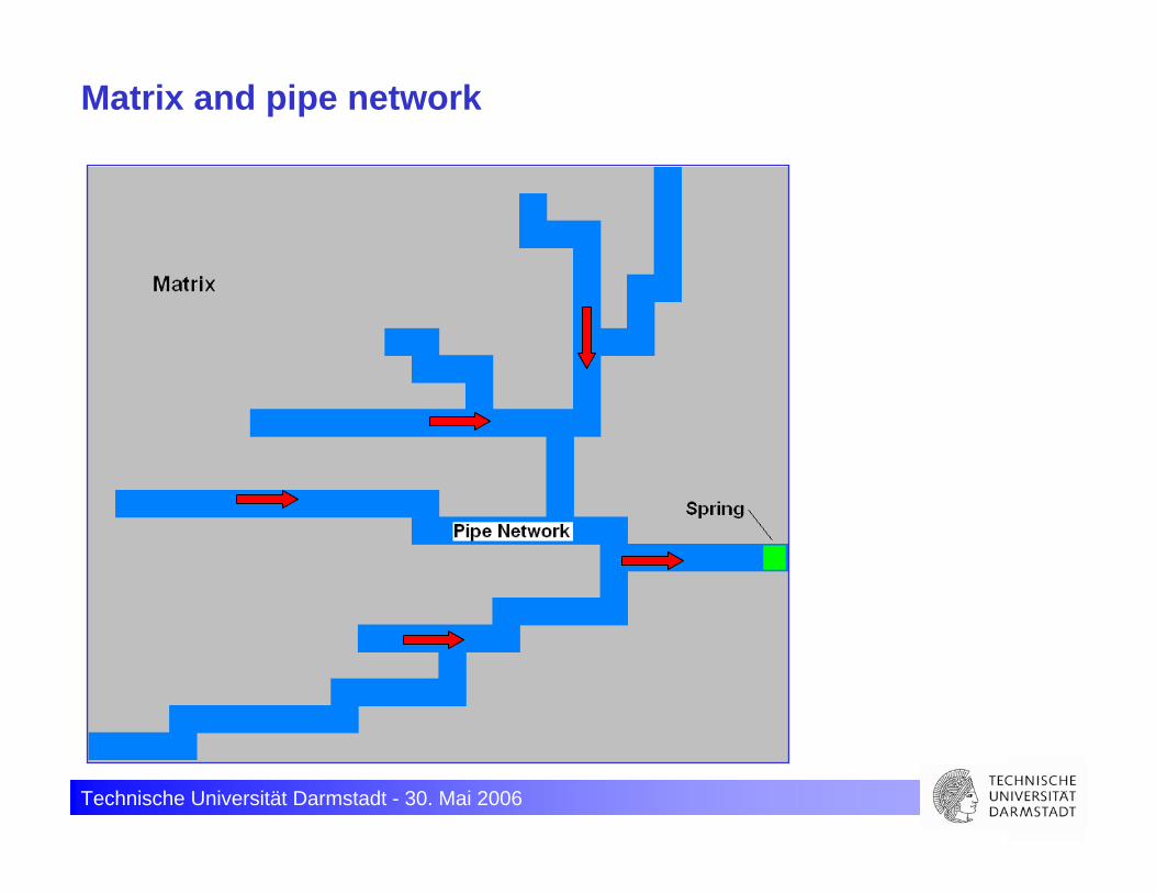
Problem: Flow in fractures and pipes

Technische Universität Darmstadt - 30. Mai 2006
Large dynamics in head and discharge
Technische Universität Darmstadt - 30. Mai 2006
Matrix and pipe network

Technische Universität Darmstadt - 30. Mai 2006
Matrix and pipe network + observation wells

Technische Universität Darmstadt - 30. Mai 2006
Interpolated head distribution

Technische Universität Darmstadt - 30. Mai 2006
Interpolated head distribution and reality

Technische Universität Darmstadt - 30. Mai 2006
Classification of fractured media
Mesh of fracturesand impermeablematrix
Fractures withpermeablematrix
Fractured systemwith minorkarstification
Conduit systemwith a karstifiedrock matrix
Granite Sandstone Limestone Karstified Limestone
Waste Disposal Water Supply

Technische Universität Darmstadt - 30. Mai 2006
Possible model approaches
Single PorosityModel
Double PorosityModel
Discretemodel
Equivalentcontinuum
Two coupledfracturesystems
Twoequivalentcontinua
Fracturenetwork and continuum

Technische Universität Darmstadt - 30. Mai 2006
Double continuum flow model
Linear exchange depends on:
• head difference• exchange coefficient
Different aquifer parameters:
• Hydraulic conductivity
• low in fissured system• high in conduit system
• Storage coefficient:
• high in fissured system• low in conduit system
Karst system Double continuum system

Technische Universität Darmstadt - 30. Mai 2006
System of coupled flow equations:
( )
( )
)t,z,y,x(fhand)t,z,y,x(fh:Solution
hhWt
hSzhk
zyhk
yxhk
x
hhWt
hSzhk
zyhk
yxhk
x
ba
babb
bb
bzz
bbyy
bbxx
baaa
aa
azz
aayy
aaxx
==
−α−+∂∂
=⎟⎟⎠
⎞⎜⎜⎝
⎛∂∂
∂∂
+⎟⎟⎠
⎞⎜⎜⎝
⎛∂∂
∂∂
+⎟⎟⎠
⎞⎜⎜⎝
⎛∂∂
∂∂
−α++∂∂
=⎟⎟⎠
⎞⎜⎜⎝
⎛∂∂
∂∂
+⎟⎟⎠
⎞⎜⎜⎝
⎛∂∂
∂∂
+⎟⎟⎠
⎞⎜⎜⎝
⎛∂∂
∂∂
000
000

Technische Universität Darmstadt - 30. Mai 2006
Parameter identification – interpretation of heads
Classification by standard deviation
heads from fracture system:
large standard deviationsame range as continuum b (conduit system)
heads from matrix system:
only one point with same standard deviation as continuum a (fissured system)

Technische Universität Darmstadt - 30. Mai 2006
Double continuum model: “Stubersheimer Alb“
• steady state model calibrationusing measured head and discharge data
⇒ distribution of hydraulicconductivity
• sensitivity study for transientflow: simulate the measuredcharacteristics to investigate theexchange behavior

Technische Universität Darmstadt - 30. Mai 2006
Transient exchange betweenfracture and matrix system
Simulation results
Continuum a: smooth curveContinuum b: large dynamics
Double continuum model showssame characteristics as measureddata
Heads
Discharge

Technische Universität Darmstadt - 30. Mai 2006
Solute Transport Modeling

Technische Universität Darmstadt - 30. Mai 2006
Application of solute transport models
• interpretation of concentration data
• mass balance of contaminants
• predictions of pollutant plumes
• design of pump and treat management
• planning of monitoring strategy
• risk assessment in case of waste disposals

Technische Universität Darmstadt - 30. Mai 2006
Simulation of a contamination plume

Technische Universität Darmstadt - 30. Mai 2006
Relation between groundwater flow and transport models

Technische Universität Darmstadt - 30. Mai 2006
Representation of transport processes
Advection
Advection + Dispersion (+ Diffusion)
Advection + Dispersion + Adsorption
Advection + Dispersion + Adsorption + Decay
Transport in 1-D-aquifer
Technische Universität Darmstadt - 30. Mai 2006
( ) )( inf
ccnquccD
tc
−−+−∇⋅∇=∂∂ σ
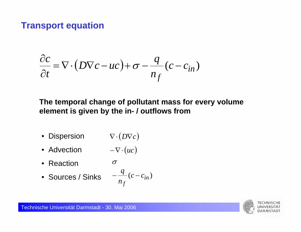
Transport equation
The temporal change of pollutant mass for every volumeelement is given by the in- / outflows from
• Dispersion
• Advection
• Reaction
• Sources / Sinks
( )cD∇⋅∇
( )uc⋅∇−
)( inf
ccnq
−−
σ

Technische Universität Darmstadt - 30. Mai 2006
1-D transport equation
Measure for the relation advective / dispersive transport is given by the PECLET-number:
xcu
xcD
tc
∂∂
−∂∂
=∂∂
2
2
uuL
DuLP
LL
eα
==
L: typical length scale of transport problem
Pe = 0 pure dispersive transport
Pe = pure advective transport∞

Technische Universität Darmstadt - 30. Mai 2006
Solution methods for transport equation
- Analytical solutionsSimple flow conditions / simple initial and boundary conditions, homogeneity
- Neglecting Diffusion / DispersionPath lines, travel times, concentration along path lines
- Numerical SolutionsGrid methods: FD, FV, FE
Particle-Tracking Methods: MOC, Random-Walk

Technische Universität Darmstadt - 30. Mai 2006
Numerical solution methods
Grid Methods:Finite Differences Finite Elements
Finite Volumes
Particle-Tracking Methods:Method of Characteristics
Random-Walk-Method

Technische Universität Darmstadt - 30. Mai 2006
Problems with grid methods
- Numerical dispersion
- Oscillations
Possible solution: grid refinement

Technische Universität Darmstadt - 30. Mai 2006
Possible solution: adaptive grid
Adaptive gridding methods consists in dynamically refining the grid size to eliminate numerical dispersion
Example of grid refinement

Technische Universität Darmstadt - 30. Mai 2006
Adaptive refinement: nested iteration

Technische Universität Darmstadt - 30. Mai 2006
Typical error indicators are
• The gradient of the solution ,
• Concentration variation between neighbor elements.
The selection of elements for refinement and coarsening is basedon an error indicator.
c∇
In case of time step methods the solution of the proceeding time step is considered.
Error indicator for adaptive griding

Technische Universität Darmstadt - 30. Mai 2006
Example of an adaptive refined grid from a simulation

Technische Universität Darmstadt - 30. Mai 2006
The Inverse Problem in Groundwater Modeling

Technische Universität Darmstadt - 30. Mai 2006
Direct problem
Given: parameters, boundary and initial conditions
Wanted: head / flow distribution (or concentration)
Usually parameters are not known completely!
Therefore:
Calibration (i.e. completion of parameters) using measurements of heads / flows (or concentration) is required.

Technische Universität Darmstadt - 30. Mai 2006
Inverse problem
Given: heads / flows, (concentrations)
Wanted: parameter distribution
Problem: ill-posednessNo unique solution may existMeasurement errors make result unreliable
Ways out: Reduction of degrees of freedom and regressionIntroduction of “a priori” knowledgeJoint use of head, flow and / or concentration measurementsEstimate of uncertainty

Technische Universität Darmstadt - 30. Mai 2006
Example for non uniqueness of the inverse problem
Q = B T (h1-h2)/L
Where:
Q: dischargeB: widthT: transmissivityh: headL: length
Identification problem of steady state calibration. Every T leads to the same head distribution, only Q varies!

Technische Universität Darmstadt - 30. Mai 2006
Criterion for goodness of fit (maximum likelihood)
Without prior knowledge minimize
or with „a priori“ knowledge
Minimization can be done manually („trial and error“) or byautomatic methods: e.g. MARQUARDT-LEVENBERG algorithm
ikcomputed
ii
measuredim wpffppS 2
1 ))((),...,( −=∑
jj
priorjjik
computedi
i
measuredim wppwpffppS ′−+−= ∑∑ 22
1 )())((),...,(
(pj parameter, fi heads or flow, wi weights)

Technische Universität Darmstadt - 30. Mai 2006
Concepts for parameterization of spatial structures
Reduction of degreesof freedom by:
Zonation (N zones)
Interpolation and pivotpoints

Technische Universität Darmstadt - 30. Mai 2006
Spatial transmissivity distribution (Jurassic karst aquifer)
Frequency distributions:all data
valleys
plateau

Technische Universität Darmstadt - 30. Mai 2006
Umm Er Radhuma aquifer system in Saudi Arabia

Technische Universität Darmstadt - 30. Mai 2006
Geological and hydrogeological units of the Umm Er Radhuma aquifer system
I R A Q
I R A N
ARABIAN GULF
QATAR
K U W A I T
Euphrates
Tigris
BAHRAIN
U. A. E.
AS SULAYYIL
AZ ZULFI
RIYADH
BURAYDAH
HAFAR AL BATIN
AN NUYRIYAH
AL KHAFJI
AD DAMMAM
AL HUFUF
BUQAYQ
SALWAH
HARAD
LAYLA
YABRIN
AL KHARJ
AL KHUBAR
AL JUBAYL
Kilometers
0 100 20050
Legend
Umm Er Radhuma
Quaternary
Neogene
Dammam
Rus
Aruma
Tdm
Tsm
Tr
Ka
Q
Tu
Ka
Ka
Tu
Tu
Tr
Tdm
Tsm
Tsm
Q
Q
Tdm
Technische Universität Darmstadt - 30. Mai 2006
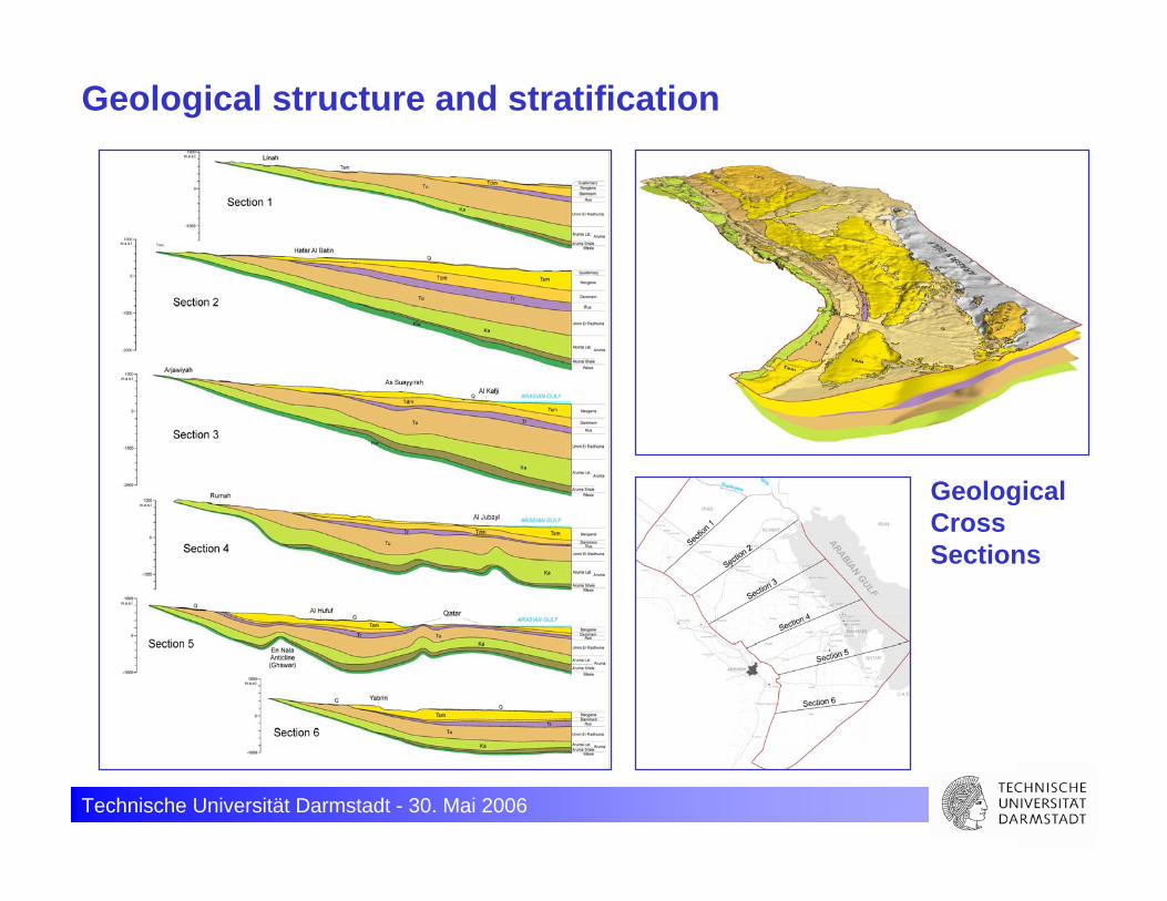
Geological structure and stratification
Geological Cross Sections

Technische Universität Darmstadt - 30. Mai 2006
Geological structure and tectonic features
Main Anticlinal Structures and Faults
Colored sub crop surface:
base of Umm Er Radhuma

Technische Universität Darmstadt - 30. Mai 2006
Vertical hydraulic conductivity distribution
Rus aquitard Dammam / Neogene

Technische Universität Darmstadt - 30. Mai 2006
Muschelkalk lithology

Technische Universität Darmstadt - 30. Mai 2006
Time needed for the change of rocks within an aquiferdepends on rock type
Important features for the Muschelkalk are:
- the dissolution of evaporites, - and the karstification of carbonate rocks.
The processes depend on the exposition to theground surface.

Technische Universität Darmstadt - 30. Mai 2006
Thickness reduction of the Mittlerer Muschelkalk by saltand sulphate dissolution

Technische Universität Darmstadt - 30. Mai 2006
Consequence:
• 50 m thickness reduction within a relative short time
• Cracking of rocks• Intensification of fractures• Acceleration of karstification

Technische Universität Darmstadt - 30. Mai 2006
What are the major processes for dissolution?
• The main factor is the exposition to the ground surface.
• The exposition to the ground surface depends on the cuesta development.

Technische Universität Darmstadt - 30. Mai 2006
“Cuesta“ development in Baden-Württemberg
Location of cuestas and rivers during Oligocene and Late Miocene (34 – 20 Ma)

Technische Universität Darmstadt - 30. Mai 2006
“Cuesta“ development in Baden-Württemberg
Location of cuestas and rivers during Upper Miocene(11 – 5 Ma)
Technische Universität Darmstadt - 30. Mai 2006
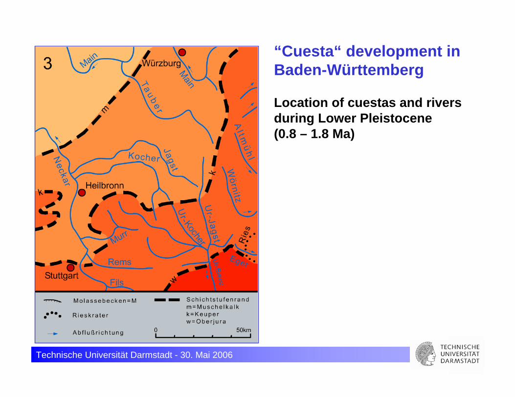
“Cuesta“ development in Baden-Württemberg
Location of cuestas and rivers during Lower Pleistocene(0.8 – 1.8 Ma)

Technische Universität Darmstadt - 30. Mai 2006
“Cuesta“ development in northern Baden-Württemberg
Cuesta development and location of Muschelkalk aquifers from Oligocene - Quarternary

Technische Universität Darmstadt - 30. Mai 2006
Consequence
• Adjacent areas within the cuesta landscape developed successively over a long time and represent different states of karstification.

Technische Universität Darmstadt - 30. Mai 2006
Present Muschelkalk aquifer systems
1 - 3: present areas of Muschelkalk aquifers
Technische Universität Darmstadt - 30. Mai 2006
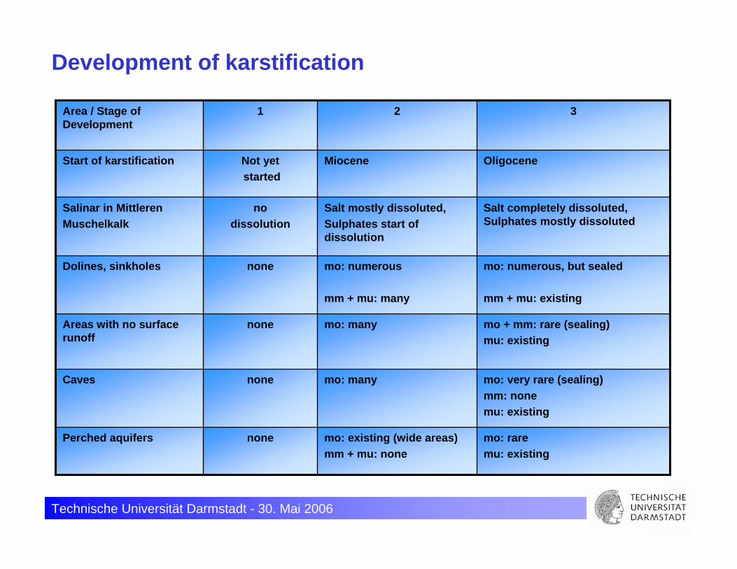
Development of karstification
mo: raremu: existing
mo: existing (wide areas)mm + mu: none
nonePerched aquifers
mo: very rare (sealing)mm: nonemu: existing
mo: manynoneCaves
mo + mm: rare (sealing)mu: existing
mo: manynoneAreas with no surface runoff
mo: numerous, but sealed
mm + mu: existing
mo: numerous
mm + mu: many
noneDolines, sinkholes
Salt completely dissoluted,Sulphates mostly dissoluted
Salt mostly dissoluted,Sulphates start of dissolution
nodissolution
Salinar in MittlerenMuschelkalk
OligoceneMioceneNot yetstarted
Start of karstification
321Area / Stage of Development

Technische Universität Darmstadt - 30. Mai 2006
Palaeo-climatology
Recharge Estimation
0
10
20
30
40
50
60
10000 8000 6000 4000 2000 0
Years Before Present
Rec
harg
e [m
m/y
]
Precipitation Fluctuations
0
100
200
300
400
500
600
700
0200040006000800010000
Years Before Present
Prec
ipita
tion
[mm
/yea
r]
BRICE 1978DIESTER-HAAS 1973
BRICE 1978
COLE 2004DIESTER-HAAS 1973VAN ZINDEREN BAKKER 1980
BRICE 1978
BRICE 1978
COLE 2004
COLE2004
VAN ZINDEREN BAKKER 1980
BRICE 1978
BRICE 1978
ISSAR2003
BRICE 1978BUTZER 1958
BARTH 1999BRICE 1978
Temperature Fluctuations
23
24
25
26
27
28
0200040006000800010000
Years Before Present
Tem
pera
ture
[°C
]

Technische Universität Darmstadt - 30. Mai 2006
Isotopes information: estimation of river infiltration
Temporal distribution of d18O in river water and groundwater
Spatial distribution of Iller infiltration

Technische Universität Darmstadt - 30. Mai 2006
Isotopes information: groundwater age
Simulated travel time to the Al Hassa oasis (mean residence time 12,000 a)
Groundwater Age Umm Er Radhuma Aquifer14C-Groundwater Age and 3H- Detection Line

Technische Universität Darmstadt - 30. Mai 2006
Modeling under uncertainty
• worst case – best case analysis
• scenario techniques
• sensitivity analysis
• stochastic modeling

Technische Universität Darmstadt - 30. Mai 2006
Stochastic modeling
Required: Parameter distribution, mean, variance, correlation length
Result: Mean, deviation, confidence limits
Methods: Monte Carlo Simulation
FOSM (First Order Second Moment)

Technische Universität Darmstadt - 30. Mai 2006
Monte Carlo method
Principle:
- generation of a large number N of equally probable random realizations of the aquifer
- the ensemble of N calculated solutions (Zi) is analyzed statistically
1
)(1
2
1
−
−==
∑∑==
N
ZZ
N
ZZ
N
ii
N
ii
σ
Technische Universität Darmstadt - 30. Mai 2006
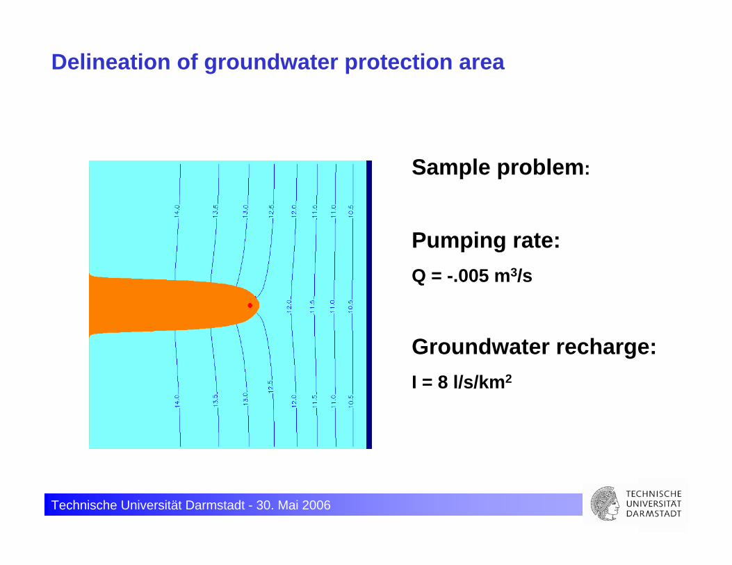
Delineation of groundwater protection area
Sample problem:
Pumping rate:Q = -.005 m3/s
Groundwater recharge:I = 8 l/s/km2

Technische Universität Darmstadt - 30. Mai 2006
Statistical analysis of field data

Technische Universität Darmstadt - 30. Mai 2006
Simulation steps using Monte Carlo method

Technische Universität Darmstadt - 30. Mai 2006
Simulation steps using Monte Carlo method
Repeated simulation of catchment areas
Unconstrained sampling
Sampling under calibration constraint

Technische Universität Darmstadt - 30. Mai 2006
Simulation steps using Monte Carlo method
Probability distribution

Technische Universität Darmstadt - 30. Mai 2006
Convergence of Monte Carlo method
A large number of realizations N may be necessary in order to get meaningful convergent statistics
Problem: this number is not known a priori !

Technische Universität Darmstadt - 30. Mai 2006
Never forget:
• a good model includes important features of reality
• a model does not replace data acquisition
• a good modeler explores the uncertainty of her/his predictions
• what we really want are robust decisions
• do not overstretch a model
• a model is not reality

Technische Universität Darmstadt - 30. Mai 2006

Technische Universität Darmstadt - 30. Mai 2006